savings and problem debt - stepchange

Page | 1

training | advice | analysis | research | data |surveys

Oxygen House

Grenadier Road

Exeter Business Park

Exeter, Devon, EX1 3LH

tel: 01392 440426

email: [email protected]

web: www.select-statistics.co.uk

Savings and Problem Debt

Author: Sarah Marley

Reviewed by: Steve Brooks

Revision Date: 27th

November 2014

Prepared for: StepChange Debt Charity Debt

Charity

Reference Number: STEP001v2

Page | 2


Executive Summary The ONS Wealth and Assets survey data suggest that cash savings are a highly statistically significant

predictor for household problem debt, with the risk of problem debt estimated to be lower for

households with higher cash savings. The relationship between savings and the risk of problem debt

was found to be non-linear, the effect being stronger for the initial cash savings held, and the effect

of additional savings decreasing with the total cash savings held.

Taking the effect of other significant risk factors into account, for a household with an average net

annual (regular) income of £25,000, the odds of problem debt is estimated to be approximately 44%

lower if the household has cash savings of £1,000, 72% lower if the household has cash savings of

£5,000, and 84% lower with cash savings of £10,000. For households with lower regular incomes, the

protective effect of savings was found to be slightly higher.

Using the model output to predict problem debt, we estimate that approximately 3.3 million

households are at risk of problem debt across Great Britain.

Increasing household cash savings to a minimum of £1,000 (for those households with lower savings

currently) reduces the number of households estimated to be at risk of problem debt by

approximately 500,000 homes (to 2.8 million). A minimum of £5,000 household cash savings further

reduces this to 1.9 million households at risk of problem debt, £10,000 to 1.3 million households and

£20,000 to 700,000 households at risk in Great Britain.

Introduction Select were pleased to be asked to undertake the statistical analysis of the Wealth and Assets survey

data by StepChange Debt Charity Debt Charity. StepChange Debt Charity Debt Charity was looking

for support in producing a detailed and statistically-based answer to the questions as to whether a

lack of savings increases the likelihood of problem debt and whether having savings might help

prevent problem debt.

The project is split into two parts:

1) Investigating any statistical link between a lack of savings and problem debt, or savings and lack

of problem debt; and

2) Estimation of

a) the levels of savings necessary to help households stay out of problem debt;

b) the number of households across the UK without this adequate level of saving; and

c) how much savings levels need to be boosted in order to prevent or minimise problem debt

in the UK.

In this report we summarise the results of the analysis and give a technical explanation of the

analysis methodology.

Data We focus the analysis on data from the Wealth and Assets Survey (WAS), a detailed, longitudinal

survey of private households in Great Britain conducted by the Social Survey Division of the Office

for National Statistics (ONS). The WAS provides considerable information on the wealth of

households and individuals, including the level, distribution, nature and type of assets (including

Page | 3


savings) and debts of all types as well as attitudes to financial planning, saving and financial advice.

Private households in Great Britain were sampled for the survey (meaning that people in residential

institutions, such as retirement homes, nursing homes, prisons, barracks or university halls of

residence, and also homeless people were not included) and data were collected via face-to-face

interviews.

Data from the most recent wave of the WAS, which were collected between July 2010 and June

2012, were obtained from the UK Data Archive (End User Licence version, for non-commercial use;

16 October 2014, 3rd Edition) (ONS, 2014). We considered including additional data in the analysis

from the Family Resources Survey (FRS) (collected by the Department for Work and Pensions), which

are also available from the UK Data Archive. However, it was not possible to match the records for

households in each of the surveys as, for anonymity, direct identifiers such as names, addresses and

other contact details were omitted from the datasets.

The WAS questionnaire was divided into two parts, one for the household and the other for each

individual within that household. All adults aged 16 years and over (excluding those aged 16-18

currently in full-time education) were interviewed in each responding household. The household

schedule was completed by one person in the household and predominantly collected household

level information such as the number, demographics and relationship of individuals to each other, as

well as information about the ownership, value and mortgages on the residence and other

household assets. The individual schedule was given to each adult in the household and asked

questions about economic status, education and employment, business assets, benefits and tax

credits, saving attitudes and behaviour, attitudes to debt, insolvency, major items of expenditure,

retirement, attitudes to saving for retirement, pensions, financial assets, non-mortgage debt, and

investments and other income.

In order to answer the questions posed in the project brief, at the requested household-level, any

individual person-level variables of interest first needed to be aggregated to the household level

prior to analysis. The WAS identifies a Household Reference Person (HRP) in each household,

according to the ONS definition. This is an individual person within the household who is identified

as a reference point for producing further derived statistics and for characterising a whole

household according to characteristics of the chosen reference person. In households with more

than one adult, the most economically active person is chosen (in the priority order: full-time job,

part-time job, unemployed, retired, other), if all adults have the same economic activity then the

eldest person is selected.

Problem Debt

Following discussion with StepChange Debt Charity Debt Charity, we agreed to base the definition of

problem debt on the self-reported burden of debt supplied in the WAS data. Two questions are

posed in the WAS regarding whether payments are a financial burden, one considering burden from

non-mortgage debt and the other burden of mortgage and other debt on the household (DBurd and

DBurdH, respectively). These questions are posed to all individuals that are surveyed in the

household with possible responses of “A heavy burden”, “Somewhat of a burden”, or “Not a

problem at all”.

Page | 4


For the purpose of this work, StepChange Debt Charity is focussed on non-mortgage debt burden,

and therefore self-reported burden from non-mortgage debt (DBurd) only was considered. We

agreed with StepChange Debt Charity to define household problem debt as a response of “A heavy

burden” from either the HRP or their partner, where applicable.

Excluding households where no response regarding self-reported burden from non-mortgage debt

was available from either the HRP or their partner (5,120 households), 1,752 out of the 16,326

remaining households (10.7%) were defined as having problem debt.

Cash/Accessible Savings

StepChange Debt Charity indicated that they would like to consider only accessible, cash savings,

rather than assets, as part of the analysis. Therefore, we only include cash/accessible savings, not

stocks, shares, bonds, household valuables, endowment policies, or other financial assets, for

example.

The total household cash/accessible savings were calculated from the WAS data by summing the

household value of cash ISAs (not including investment ISAs which includes stocks, shares, life

insurance, corporate bonds and PEPs), informal savings (e.g., cash or loose change, given to

someone else to look after and save for you, etc.), current accounts in credit and savings accounts

(e.g., Savings or deposit account with a bank or building society, National Savings Easy Access

[Ordinary] Account, etc.).

Other Risk Factors

In addition to cash savings, we want to account for other potential risk factors in the analysis. The

WAS includes many additional variables that could be considered as other potential risk factors for

problem debt. StepChange Debt Charity have conducted some background research on factors

associated with over-indebtedness, including individual, economic and attitudinal variables. We have

used this information (through the “Why might individuals become over-indebted” document

provided by StepChange Debt Charity) to inform the independent variables to be selected from the

WAS for potential inclusion in the modelling (see the Methods section below for further details).

It was not possible to include national finance variables in the analysis (e.g., interest rates, housing

costs, etc.), due both to potential issues with, e.g., highly correlated variables, as well as the narrow

period of time that the survey data covers which limits the range of values observed for these

variables. Disney, et al. (2008) argue that national finance variables are not influential once

individual factors are taken into account and StepChange Debt Charity agreed that the focus should

be on the individual and attitudinal variables, therefore the economic variables were dropped from

this analysis.

Details of the variables selected from the WAS data, matched against the potential risk factors

identified by StepChange Debt Charity are provided in Table 1. Household Net Annual (regular)

income includes usual net employment earnings for employees (main and second job), net annual

profit or loss from self-employment, annual income from benefits, net annual income from

occupational or private pensions, net annual income from state pension, net annual income from

investment, and net annual other regular income (such as rental income).

Page | 5


Some additional attitudinal variables were also considered (e.g., “I find it more satisfying to spend

money than to save it for the long term”, and “Choice between a guaranteed payment of one

thousand pounds and a one in five chance of winning ten thousand”) but it was not possible to

include all of these due to aliasing with other variables. Aliasing refers to effects in linear models

that cannot be estimated independently of the terms which occur earlier in the model as there is a

linear dependency amongst the variables. This means that the variables are predictive of each other

(as well as of problem debt). For example, if a continuous variable is perfectly correlated with

another variable, then the terms are aliased – the second variable adds nothing to the descriptive

power of the model once the first variable has been included. For a categorical variable, if, for

example, all respondents who “Agree strongly” to the statement ‘I find it more satisfying to spend

money than to save it for the long term’ also “Disagree strongly” with the statement ‘I always make

sure that I have money saved for a rainy day’ then these terms would be aliased. Aliasing arises most

commonly when there are a lot of categorical factors included in a model. In this case, it’s likely due

to a combination of intrinsic and extrinsic aliasing, the former arising because of dependencies

inherent in the definition of the variables in the survey, and the latter arising from the nature of the

data.

Where appropriate, e.g., for the attitudinal questions on money, the explanatory variables were

based on the HRP’s responses to the questionnaire, or the person who makes the financial decisions

in the household (if this was the HRP’s partner rather than the HRP).

Sparse Categories

For some of the categorical variables in the data set, some of the categories had very few responses

(these categories were generally missing data responses such as “Don’t know”, “No answer”, “Does

not apply”, “Error/Partial”). In these cases it is unlikely that there would be sufficient observations to

estimate the effect and statistical significance of that category reliably. In order to retain as many

data points as possible and maximise the predictive power of the analysis, we grouped these

responses into a single response category in order to remove the sparse groupings without excluding

any observations. This approach also enabled us to use the model to predict the risk of problem debt

for all households in the survey (and extrapolate to all households in Great Britain) which requires

that all potential response categories are retained in the model.

Methods

Model Fitting and Selection

We analysed the data using a logistic regression model to explore the potential link between savings

and problem debt, with presence/absence of problem debt as the dependent variable. This uses a

logistic transformation to express the probability of problem debt as a linear function of the

independent variables. This allows us to investigate the potential effect of cash/accessible savings on

the risk of having problem debt and also account for (and estimate the effects of) other

independent variables.

Separation

When developing the logistic regression model, so-called quasi-separation was identified. Separation

occurs in logistic regression when the binary outcome variable (presence/absence of problem debt)

can be separated by an independent variable. Complete separation occurs when the separation is

Page | 6


perfect whereas quasi-complete separation happens when the outcome is separated to a certain

degree, for example where all of the responses for one factor of a categorical variable (rather than

all factors) have the same outcome. This can happen even when the underlying model parameters

are relatively small (in absolute terms) (Heinze & Schemper, 2002). In the WAS survey results, all of

those households with very high cash savings had an absence of problem debt causing partial

separation.

In the presence of separation, standard logistic regression models fitted via maximum likelihood can

produce infinite or biased estimates. Separation is a common problem in logistic regression which is

more likely to occur with smaller sample sizes, with more dichotomous independent variables, and

with more extreme odds ratios and with larger imbalances in their distribution. Biased estimates can

also occur in the absence of separation, when there are relatively small sample sizes for some

categories. This was also a possibility in the current analysis, where there were sometimes relatively

small groups of responses to a question that were recorded as “Does not know”, “Does not apply”,

“Error/partial”, etc., as discussed above.

There are a few options for dealing with this in the analysis. Firstly, we could omit those cases

causing separation from the analysis. However, this is not necessarily appropriate as it won’t provide

any information about the effect of this potentially important independent variable and also doesn’t

allow us to adjust the effects of the other independent variables for the effect of this variable. This

would also mean throwing away data, thereby reducing the predictive power of the modelling and,

as discussed above, in order to use the model to predict the risk of problem debt for all households

in the survey (and extrapolate to all households in Great Britain) all potential response categories

needed to be retained in the model.

To address the separation and small sample sizes identified, instead we apply Firth's bias reducing,

penalised maximum likelihood logistic regression (Fisher, 1992, 1993). This is an alternative model

fitting approach which reduces the bias of the maximum likelihood estimates and guarantees the

existence of the estimates (even when finite standard maximum likelihood estimates may not exist)

(Heinze, 1999; Heinze and Schemper, 2002).

Stepwise Regression Algorithm

We used a backward stepwise regression algorithm which begins with the model including all

potential independent variables, and then successively removes them from the model in order to

determine the model that provides the best fit. The model fit is determined using penalised

likelihood ratio tests (with a 5% significance level, i.e., requiring the probability that the observed

effect is due to chance alone is less than 5%) ensuring that only variables that have a substantial

effect on the performance of the model are included.

Penalised likelihood ratio tests are used, rather than more commonly applied information criterion

(such Akaike’s Information Criterion [AIC]) or Wald's tests, as they have been shown to often

perform better for Firth's logistic regression method (Heinze and Schemper, 2002). Similarly, profile

penalised likelihood confidence intervals are preferred to Wald confidence intervals.

Variable Transformations

In some cases multiple similar variables were considered for a particular risk factor, e.g., for Age of

HRP or partner, two different bandings of age categories were explored (15 Age bands: 0-16, 17-19,

Page | 7


20-24, 25-29, 30-34, 35-39, 40-44, 45-49, 50-54, 55-59, 60-64, 65-69, 70-74, 75-79, 80+; and 9 Age

bands: 0-15, 16-24, 25-24, 35-44, 45-54, 55-64, 65-74, 75-84, 85+) and for Number of dependent

children a continuous and a banded variable (1, 2, 3, 4, or 5+) were considered. In these cases, we

explored uni-variable models for these confounders to assess which variable was most informative

in characterising the relationship between that risk factor and problem debt. That variable was then

retained in the stepwise regression analysis.

For the continuous variables (Household Net Annual (regular) income and Cash/accessible savings) a

number of transformations were considered to determine which best fit the shape of the

relationship with the risk of problem debt. Raw, log, square-root and banded (for income only)

transformations were considered. For both variables, the square-rooted transformation was most

informative in characterising the relationship between that risk factor and problem debt.

Interactions

In addition to the main effects for each of the independent variables, we also considered including

interactions between the risk factors in the model (where the effect of one variable might have an

effect on, i.e., interact with, the effect of another variable).

It wasn’t possible to consider all two-way interactions, given the number of categorical variables

considered. The model would have been over-fitted, i.e., had too many parameters compared to

the number of observations used for fitting. A generally accepted rule-of-thumb for multiple logistic

regression is that 10 ‘events’ (i.e., occurrences of problem debt in this case) are needed per

coefficient in the model (Peduzzi, et al., 1996). In the WAS wave 3 data, approximately 1,700 of the

households reported problem debt, so applying this rule-of-thumb, we could include up to

approximately 170 coefficients in the model. Just including each of the independent variables

identified in Table 1, equates to 86 coefficients in the model. Therefore, we restricted ourselves to

considering interactions only between cash savings and the other independent variables. Of these,

we determined that only an interaction between cash savings and household income should be

included in the model, as all other interactions with cash savings had little effect on the performance

of the model in predicting problem debt and had limited practical interpretation.

GB Prediction and Scenario Testing

Having determined the final model, it is then used to address the secondary objectives of the

project.

We apply the model to predict the probability of problem debt for all households in the complete

WAS dataset (including households with missing responses to the self-reported burden debt

questions). The WAS data includes cross-sectional analysis weights that are used to account for the

sampling design and non-response in the survey in order to ensure that the data are representative

of households and individuals in Great Britain. Applying these weights and then summing the

weighted probabilities, we can extrapolate from the predicted probabilities of problem debt for

those households included in the survey to the number of households predicted to be at risk of

problem debt across Great Britain.

We can then carry out scenario testing to explore the effect of increasing household cash savings (to

a minimum of £1,000, £5,000, £10,000 or £20,000, for example) on the estimated levels of problem

debt in Great Britain.

Page | 8


Although we would usually like to provide estimates of the uncertainty of these predictions (via

standard errors and confidence intervals, for example), this is not possible without survey design

information (details of stratification, clustering and calibration, as well as weights). The WAS has a

complex design in that it employs a two-stage, stratified sample of addresses with oversampling of

the wealthier addresses at the second stage and implicit stratification in the selection of primary

sampling units. Such information could not be provided with the datasets for statistical disclosure

reasons and therefore these estimates of uncertainty cannot be provided.

All analyses were performed in the statistical software package R version 3.1.1 (R Core Team, 2013).

The logistf package was used to implement Firth’s penalised maximum likelihood logistic regression

method (Heinze and Ploner, 2004; Ploner, et al., 2013).

Results The results of the analyses described above are summarised in this section.

Statistical Link between a Lack of Savings and Problem Debt

The results of the multiple logistic regression modelling to assess the collective predictive accuracy

of the independent variables for household problem debt are provided in Table 2 and Table 3.

Table 2 summarises the steps taken in determining the optimal model. The stepwise regression

algorithm begins with the full model (including all independent variables considered) and removes

one variable at a time in order to determine the model with the best fit. The final model from the

stepwise regression analysis includes:

National Statistics Socio-Economic Classification (Nssec) of HRP or partner;

Employment Status of HRP or partner;

Number of dependent children;

De facto marital status of HRP/partner;

Tenure;

General Health;

Longstanding illness, disability or infirmity;

Opinion on whether to buy on credit;

Whether organised when managing money;

Guaranteed £1,000 today or £1,100 next year;

Type of household;

OAC (Output Area Classification) Supergroup;

Household Net Annual (regular) income;

Cash/accessible savings; and

Income & Cash savings interaction.

The corresponding coefficient values are given in Table 3. These variables provide the most

informative combination of explanatory variables for problem debt. They are independently

predictive of the outcome; each contributing to the predictive performance of the model in

explaining differences in the odds of problem debt between households. The variables dropped from

the model may well be individually predictive of problem debt, but do not substantially contribute to

the predictive performance of the final model given the other variables available. A penalised

Page | 9


likelihood ratio test for the overall statistical significance of each variable as an independent

predictor of problem debt is provided in Table 2.

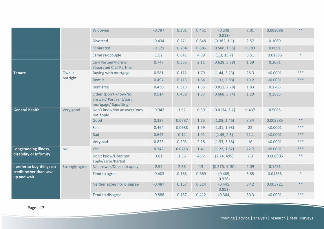
Coefficients and odds ratios from the final model along with penalised likelihood ratio tests of the

statistical significance of the odds ratio for each corresponding variable and factor level are provided

in Table 3. For a categorical variable, the odds ratio represents the odds of problem debt for that

category compared to the odds of a reference-level category of that variable. For a continuous

variable, the odds ratio represents the change in the odds per unit increase in that variable.

We find that, for example, the HRP being unemployed is associated with an increase in the odds of

problem debt of 72% compared to the HRP being employed (p=0.0003). Having dependent children

is associated with an increased odds by 73% for one child compared to none (p=0.0369) and by

423% for 5+ children compared to none (p=0.0001), for example. Renting rather than owning the

property outright is estimated to be associated with an increase in the odds of household problem

debt by 64% (p<0.0001). See Table 3 for the estimated effects of the remaining independent

variables.

The data suggest that cash savings are a highly statistically significant predictor for household

problem debt (p<0.0001). The risk of problem debt is estimated to be lower for households with

higher cash savings. The relationship between savings and the risk of problem debt was found to be

non-linear, the effect being stronger for the initial cash savings held (i.e., some versus none), and the

effect of additional savings decreasing with the total cash savings held. The model relates the log

odds of problem debt to the square-rooted cash savings held. Figure 1 and Figure 2 show the

modelled effect of cash savings on the odds of having problem debt for a household with the

average (median) observed net annual (regular) income (approx. £25,000). Figure 1 shows the

relationship for cash savings up to £50,000, and Figure 2 provides a “zoomed-in” version of the same

plot for cash savings up to £10,000.

We can see that, as the cash savings increase (along the x-axis), the gain in the percentage reduction

in the risk of problem debt decreases, gradually levelling off as we hit ‘high’ savings values. Taking

the effect of the other risk factors into account, the odds of problem debt is estimated to be

approximately 44% lower if the household has cash savings of £1,000, 72% lower if the household

has cash savings of £5,000 and 84% lower if the household has cash savings of £10,000, for example.

These figures are for a household with an average net annual (regular) income of £25,000. For

households with a lower regular income, the protective effect of savings was found to be slightly

higher (see the Income & Cash savings interaction term in Table 3; p=0.0017). This interaction effect

is small relative to the main effect of having cash savings. In Figure 3 and Figure 4, we show the

effect of cash savings on the risk of problem debt for a range of household regular incomes (based

on the 10th, 25th, 50th, 75th and 90th deciles of household net annual (regular) income observed in the

WAS). Figure 3 shows the relationship for cash savings up to £50,000, and Figure 4 provides a

“zoomed-in” version of the same plot for cash savings up to £10,000. The corresponding estimates

are provided in Table 4.

Summing the predicted probabilities for the households with non-missing responses to the self-

reported burden debt questions in the WAS, the model-predicted number of households with

Page | 10


problem debt is 1,767 households (10.8%), which is similar to the number actually observed (1,752;

10.7%).

Problem Debt in Great Britain

Given the coefficients in Table 3, the probability of problem debt under the final model can be

estimated for any household (given the corresponding values for each independent variable).

Applying the final model to the complete WAS dataset and then using the cross-sectional analysis

weights to calculate the weighted sum of the predicted probabilities, we estimate that

approximately 3.3 million households are at risk of problem debt across Great Britain.

Increasing household cash savings to a minimum of £1,000 reduces the number of households

estimated to be at risk of problem debt by approximately 500,000 homes (to 2.8 million). An

estimated 7.1 million households in Great Britain have less than £1,000 in cash savings, increasing

their levels of savings to £1,000 per household would cost approximately £5,360 million.

Further increasing household cash savings to a minimum of £5,000, the number reduces to

approximately 1.9 million households. A minimum of £10,000 household cash savings further

reduces this to 1.3 million households at risk of problem debt, and £20,000 to 700,000 households at

risk in Great Britain.

Page | 11


Tables

Category Potential Confounder WAS Variable Details/Categories

Individual Unemployed National Statistics Socio-Economic Classification (NSSEC) of HRP or partner

Never worked/long term unemployed

Managerial & prof. occupations

Intermediate occupations

Routine & manual occupations

Not classified

Employment Status of HRP or partner Employee

Self-employed

Unemployed

Student

Looking after family home

Sick or disabled

Retired

Other

Low wage income

Household Net Annual (regular) income £’s

Age Age of HRP or partner Years

New child Dependent child under 5 Yes

No

Number of dependent children Count

Relationship breakdown/Being single

De facto marital status of HRP/partner Married

Cohabiting

Page | 12


Single

Widowed

Divorced

Separated

Same sex couple

Civil Partner

Former Separated Civil Partner

Being a tenant Tenure Own it outright

Buying with mortgage

Part rent/part mortgage

Rent it

Rent-free

Squatting

No current account Whether has current account Does not have current account

Has current account

Ill health General health Very good

Good

Fair

Bad

Very bad

Longstanding illness, disability or infirmity Yes

No

Don't know / no opinion

Attitudinal Propensity to impulsive credit Opinion on whether to buy on credit (I prefer to buy Strongly agree

Page | 13


use things on credit rather than save up and wait) Tend to agree

Neither agree nor disagree

Tend to disagree

Strongly disagree

Don’t know/no opinion

Poor control over finances/Relaxed attitude to money management

Whether organised when managing money Agree strongly

Tend to agree

Tend to disagree

Disagree strongly

Don't know, no opinion

Credit 'myopia' (focus on short-term gain over long-term good)

Guaranteed £1,000 today or £1,100 next year £1,000 today

£1,100 next year

Additional demographics

- Type of household Single person over State Pension Age (SPA)

Single person below SPA

Couple over SPA

Couple below SPA

Couple, one over one below SPA

Couple and dependent children

Couple and non-dependent children only

Lone parent and dependent children

Lone parent and non-dependent children only

More than 1 family, other household types

OAC (Output Area Classification) Supergroup Rural Residents

Cosmopolitans

Page | 14


Table 1: Details of the additional independent variables considered in the analysis. Note: Categories relating to essentially missing data (e.g., Does not apply, Error/Partial) have been omitted.

Ethnicity Central

Multicultural Metropolitans

Urbanites

Suburbanites

Constrained City Dwellers

Hard-Pressed Living

Level of highest educational qualification for HRP or partner

Has qualification, degree level or above

Has qualification, other level

Has qualification, doesn’t know level

No qualifications

Page | 15


Drop 1 term p-value Significance

Step 1 Whether has current account 0.44655

Step 2 Dependent child under 5 0.38642

Step 3 Age of HRP or partner 0.22313

Step4 Level of highest educational qualification for HRP or partner 0.15825

Final Model National Statistics Socio-Economic Classification (Nssec) of HRP or partner 0.00616 **

Employment Status of HRP or partner <0.0001 ***

Number of dependent children 0.00189 **

De facto marital status of HRP/partner <0.0001 ***

Tenure <0.0001 ***

General Health <0.0001 ***

Longstanding illness, disability or infirmity <0.0001 ***

Opinion on whether to buy on credit <0.0001 ***

Whether organised when managing money <0.0001 ***

Guaranteed £,1000 today or £1,100 next year <0.0001 ***

Type of household <0.0001 ***

OAC (Output Area Classification) Supergroup <0.0001 ***

Household Net Annual (regular) income <0.0001 ***

Cash/accessible savings <0.0001 ***

Income & Cash savings interaction 0.00170 **

Table 2: Summary of the steps taken within the stepwise regression algorithm. p-values are for penalised likelihood ratio tests. Significance indicates the following: *** p-value < 0.001; ** p-value < 0.01; * p-value < 0.05; . p-value < 0.1.

Page | 16


Variable Reference Level

Factor Comparison Coefficient SE OR OR 95% CI Chi-square statistic

p-value Significance

- - (Intercept) -0.205 0.406 0.255 0.6135

National Statistics Socio-Economic Classification (Nssec) of HRP or partner

Managerial & prof. occupations

Does not apply 0.0543 0.314 1.06 (0.558, 1.91) 0.03 0.8624

Intermediate occupations 0.0631 0.091 1.07 (0.89, 1.27) 0.479 0.489

Routine & manual occupations

0.0384 0.0764 1.04 (0.895, 1.21) 0.253 0.6151

Never worked/long term unemployed

0.249 0.187 1.28 (0.889, 1.85) 1.78 0.1826

Not classified 1.28 0.333 3.59 (1.88, 6.92) 15 0.000107 ***

Employment Status of HRP or partner

Employee Does not apply/Other 0.306 0.291 1.36 (0.757, 2.36) 1.09 0.2969

Self-employed 0.213 0.116 1.24 (0.982, 1.55) 3.28 0.07023 .

Unemployed 0.544 0.15 1.72 (1.29, 2.31) 13.1 0.0002883 ***

Student -0.246 0.411 0.782 (0.343, 1.71) 0.371 0.5424

Looking after family home 0.328 0.154 1.39 (1.02, 1.87) 4.49 0.03419 *

Sick or disabled 0.0546 0.133 1.06 (0.814, 1.37) 0.17 0.6799

Retired -0.429 0.149 0.651 (0.485, 0.871)

8.37 0.003808 **

Number of dependent children

None 1 0.547 0.265 1.73 (1.03, 2.91) 4.35 0.03693 *

2 0.728 0.269 2.07 (1.23, 3.52) 7.49 0.006218 **

3 0.736 0.283 2.09 (1.2, 3.64) 6.9 0.008619 **

4 0.77 0.339 2.16 (1.11, 4.19) 5.16 0.02307 *

5+ 1.65 0.432 5.23 (2.27, 12.2) 15 0.000108 ***

De facto marital status of HRP/partner

Married Cohabiting 0.282 0.0959 1.33 (1.1, 1.6) 8.47 0.003618 **

Single -0.549 0.267 0.578 (0.343, 0.976)

4.2 0.04039 *

Page | 17


Widowed -0.797 0.301 0.451 (0.249, 0.813)

7.01 0.008086 **

Divorced -0.434 0.271 0.648 (0.382, 1.1) 2.57 0.1089

Separated -0.121 0.284 0.886 (0.508, 1.55) 0.183 0.6691

Same sex couple 1.52 0.641 4.59 (1.3, 15.7) 5.51 0.01896 *

Civil Partner/Former Separated Civil Partner

0.747 0.565 2.11 (0.628, 5.78) 1.59 0.2071

Tenure Own it outright

Buying with mortgage 0.581 0.112 1.79 (1.44, 2.23) 28.3 <0.0001 ***

Rent it 0.497 0.115 1.64 (1.31, 2.06) 19.2 <0.0001 ***

Rent-free 0.438 0.313 1.55 (0.812, 2.78) 1.83 0.1763

Other (Don’t know/No answer/ Part rent/part mortgage/ Squatting)

0.514 0.438 1.67 (0.668, 3.74) 1.29 0.2565

General health Very good Don’t know/No answer/Does not apply

-0.942 1.52 0.39 (0.0134, 6.2) 0.437 0.5085

Good 0.227 0.0787 1.25 (1.08, 1.46) 8.34 0.003885 **

Fair 0.464 0.0988 1.59 (1.31, 1.93) 22 <0.0001 ***

Bad 0.645 0.14 1.91 (1.45, 2.5) 21.1 <0.0001 ***

Very bad 0.823 0.203 2.28 (1.53, 3.38) 16 <0.0001 ***

Longstanding illness, disability or infirmity

No Yes 0.342 0.0716 1.41 (1.22, 1.62) 22.7 <0.0001 ***

Don't know/Does not apply/Error/Partial

3.81 1.36 45.2 (2.74, 495) 7.3 0.006905 **

I prefer to buy things on credit rather than save up and wait

Strongly agree No answer/Does not apply 2.95 2.38 19 (0.376, 4130) 2.09 0.1481

Tend to agree -0.403 0.165 0.669 (0.485, 0.926)

5.85 0.01558 *

Neither agree nor disagree -0.487 0.167 0.614 (0.445, 0.853)

8.42 0.003721 **

Tend to disagree -0.888 0.157 0.412 (0.304, 30.3 <0.0001 ***

Page | 18


0.561)

Strongly disagree -0.833 0.153 0.435 (0.324, 0.588)

28 <0.0001 ***

Don’t know/No opinion -0.481 0.455 0.618 (0.246, 1.46) 1.17 0.2795

Whether organised when managing money

Agree strongly No answer/Does not apply -1.87 3.04 0.154 (0.000596, 38.7)

0.625 0.4291

Don't know, no opinion 0.388 0.258 1.47 (0.88, 2.41) 2.2 0.1377

Tend to agree 0.214 0.0736 1.24 (1.07, 1.43) 8.54 0.003476 **

Tend to disagree 0.435 0.0965 1.54 (1.28, 1.87) 20 <0.0001 ***

Disagree strongly 0.778 0.117 2.18 (1.73, 2.74) 42.9 <0.0001 ***

Guaranteed £1000 today or £1,100 next year

£1,000 today No answer/Does not apply -0.589 2.73 0.555 (0.00207, 28.6)

0.0746 0.7847

£1,100 next year -0.436 0.0892 0.647 (0.542, 0.769)

25.2 <0.0001 ***

Don't know, no opinion -0.757 0.433 0.469 (0.19, 1.03) 3.5 0.06139 .

Type of household Single person over State Pension Age (SPA)

Single person below SPA 0.0905 0.182 1.09 (0.768, 1.57) 0.248 0.6184

Couple over SPA -0.601 0.327 0.548 (0.288, 1.04) 3.37 0.06631 .

Couple below SPA -0.302 0.316 0.74 (0.399, 1.37) 0.911 0.3398

Couple, one over one below SPA

0.174 0.337 1.19 (0.614, 2.3) 0.267 0.6053

Couple and dependent children

-0.436 0.348 0.647 (0.326, 1.28) 1.58 0.2091

Couple and non-dependent children only

0.221 0.324 1.25 (0.661, 2.35) 0.465 0.4952

Lone parent and dependent children

0.0286 0.32 1.03 (0.549, 1.92) 0.00803 0.9286

Lone parent and non-dependent children only

0.714 0.211 2.04 (1.35, 3.09) 11.3 0.000775 ***

More than 1 family, other 0.41 0.255 1.51 (0.908, 2.47) 2.53 0.1119

Page | 19


household types

OAC (Output Area Classification) Supergroup

Rural Residents

Cosmopolitans 0.188 0.195 1.21 (0.819, 1.76) 0.92 0.3374

Ethnicity Central 0.574 0.16 1.78 (1.3, 2.43) 12.8 0.0003438 ***

Multicultural Metropolitans 0.300 0.125 1.35 (1.06, 1.73) 5.86 0.01549 *

Urbanites 0.044 0.12 1.04 (0.827, 1.32) 0.135 0.7132

Suburbanites -0.0141 0.121 0.986 (0.779, 1.25) 0.0135 0.9076

Constrained City Dwellers -0.0327 0.135 0.968 (0.744, 1.26) 0.0591 0.8079

Hard-Pressed Living -0.0584 0.115 0.943 (0.754, 1.18) 0.257 0.6121

Household Net Annual (regular) income

- √(income) -0.00694 0.000866

0.993 (0.991, 0.995)

48.6 <0.0001 ***

Cash/accessible savings - √(Savings) -0.0228 0.00111 0.977 (0.975, 0.98) Inf <0.0001 ***

Income & Cash savings interaction

- √(Income) x √(Savings) 2.97E-05 2.25E-06

1 (1, 1) 9.84 0.001704 **

Table 3: Coefficients and odds ratios for the final logistic regression model. SE = Standard Error; OR = Odds Ratio; CI = Confidence Interval. Chi-square statistic is the test statistic for a penalised likelihood ratio test of the significance of the odds ratio for the corresponding factor. Significance indicates the following: *** p-value < 0.001; ** p-value < 0.01; * p-value < 0.05; . p-value < 0.1.

Cash Savings

Income £0 £1k £2k £3k £4k £5k £6k £7k £8k £9k £10k £15k £20k £25k £30k £35k £40k £45k £50k

£10,000 0 46.6 58.8 66.2 71.5 75.4 78.5 81.0 83.0 84.8 86.2 91.2 93.9 95.7 96.8 97.6 98.1 98.5 98.8

£16,000 0 45.2 57.3 64.8 70.0 74.0 77.1 79.7 81.8 83.6 85.1 90.3 93.2 95.1 96.3 97.2 97.8 98.2 98.6

£25,000 0 43.6 55.5 62.9 68.2 72.2 75.4 78.0 80.2 82.1 83.6 89.1 92.3 94.3 95.7 96.6 97.3 97.9 98.3

£40,000 0 41.3 53.0 60.3 65.6 69.6 72.9 75.6 77.9 79.8 81.5 87.3 90.8 93.0 94.6 95.7 96.6 97.2 97.7

£58,000 0 39.0 50.3 57.6 62.8 66.9 70.2 73.0 75.3 77.3 79.1 85.3 89.1 91.6 93.4 94.6 95.6 96.4 97.0

Table 4: Estimated percentage reduction in the log odds of problem debt versus cash savings, up to £50,000, for a range of household net (regular) annual incomes.

Page | 20


Figures

Figure 1: Plot of the relationship between cash savings, up to £50,000, and the risk of problem debt for a household with a net (regular) annual income of £25,000 under the final model.

Figure 2: Plot of the relationship between cash savings, up to £10,000, and the risk of problem debt for a household with a net (regular) annual income of £25,000 under the final model.

Page | 21


Figure 3: Plot of the relationship between cash savings, up to £50,000, and the risk of problem debt for a range of household net (regular) annual incomes under the final model.

Figure 4: Plot of the relationship between cash savings, up to £10,000, and the risk of problem debt for a range of household net (regular) annual incomes, under the final model.

Page | 22


Appendix

References

Firth, D. (1992) Bias reduction, the Jeffreys prior and GLIM. Fahrmeir, L., Francis, B., Gilchrist, R.,

Tutz, G., editors. Advances in GLIM and Statistical Modelling. Springer.

Firth, D. (1993) Bias reduction of maximum likelihood estimates. Biometrika, 80:27-38.

Heinze, G. (1999): "The application of Firth's procedure to Cox and logistic regression", Technical

Report 10/1999, Section for Clinical Biometrics, CeMSIIS, Medical University of Vienna.

Heinze, G., Schemper, M. (2002) A solution to the problem of separation in logistic regression.

Statistics in medicine, 21:2409-2419.

Heinze, G., Ploner M. (2004). Technical Report 2/2004: A SAS-macro, S-PLUS library and R package to

perform logistic regression without convergence problems. Section of Clinical Biometrics,

Department of Medical Computer Sciences, Medical University of Vienna, Vienna, Austria. URL

http://www.meduniwien.ac.at/user/georg.heinze/techreps/tr2_2004.pdf.

Office for National Statistics (ONS). Social Survey Division, Wealth and Assets Survey, Waves 1-3, 2006-2012 [computer file]. 3rd Edition. Colchester, Essex: UK Data Archive [distributor], October 2014. SN: 7215, http://dx.doi.org/10.5255/UKDA-SN-7215-3

Peduzzi, P., Concato, J., Kemper, E., Holford, E., and Feinstein, A. (1996) A simulation study of the

number of events per variable in logistic regression analysis. Journal of Clinical Epidemiology,

Volume 49, Issue 12, pp. 1373-1379.

Ploner M, Dunkler D, Southworth H, Heinze G: logistf: Firth’s bias reduced logistic regression. R

package version 2.1. http://CRAN.R-project.org/package=logistf, 2013.

R Core Team (2013). R: A language and environment for statistical computing. R Foundation for

Statistical Computing, Vienna, Austria. URL http://www.R-project.org/.

http://cemsiis.meduniwien.ac.at/fileadmin/msi_akim/CeMSIIS/KB/programme/tr10_1999.pdf

http://cran.r-project.org/package=logistf

savings and problem debt - stepchange

Documents