sc434l dvcc-tutorial 2 - ut arlington – uta · sc434l_dvcc-tutorial 2 statistical redundancy and...
TRANSCRIPT
SC434L_DVCC-Tutorial 2 Statistical Redundancy and Image
Measures
Dr H.R. Wu
Associate Professor
Audiovisual Information Processing and Digital Communications
Monash Universityhttp://www.csse.monash.edu.au/~hrw
Email: [email protected]
and
Computer EngineeringNanyang Technological University
Email: [email protected]
16 April 2002©H.R. Wu
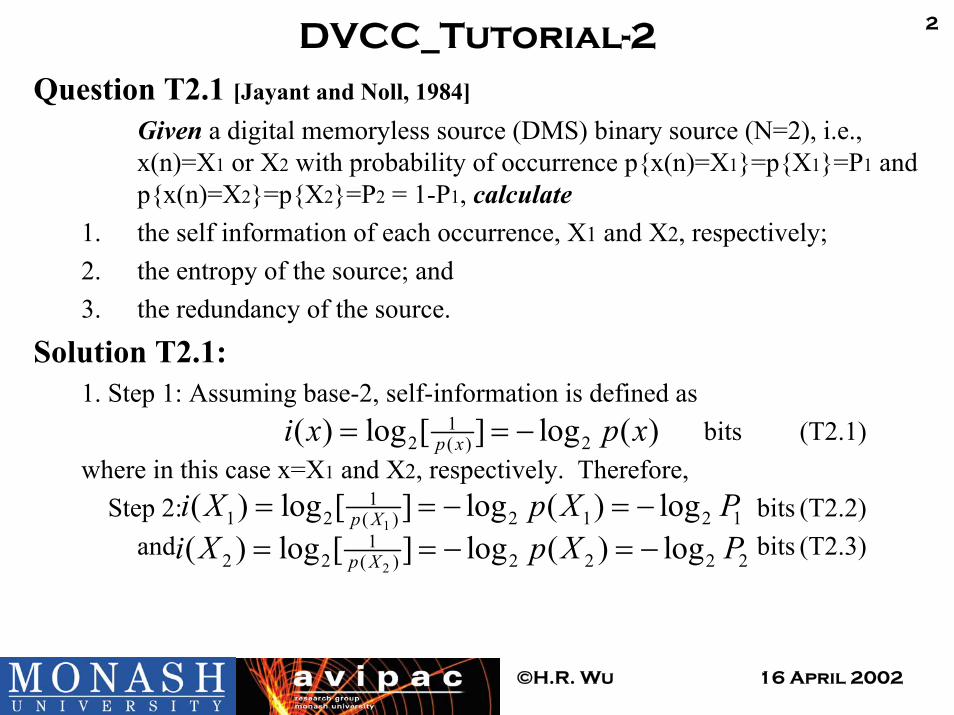
2DVCC_Tutorial-2Question T2.1 [Jayant and Noll, 1984]
Given a digital memoryless source (DMS) binary source (N=2), i.e., x(n)=X1 or X2 with probability of occurrence p{x(n)=X1}=p{X1}=P1 and p{x(n)=X2}=p{X2}=P2 = 1-P1, calculate
1. the self information of each occurrence, X1 and X2, respectively; 2. the entropy of the source; and 3. the redundancy of the source.
Solution T2.1:1. Step 1: Assuming base-2, self-information is defined as
bits (T2.1)where in this case x=X1 and X2, respectively. Therefore,
Step 2: bits (T2.2)and bits (T2.3)
12 2( )( ) log [ ] log ( )p xi x p x= = −
1
11 2 2 1 2 1( )( ) log [ ] log ( ) logp Xi X p X P= = − = −
2
12 2 2 2 2 2( )( ) log [ ] log ( ) logp Xi X p X P= = − = −

16 April 2002©H.R. Wu
3DVCC_Tutorial-2Solution T2.1:
2. Step 1: Assuming base-2, the entropy of the source is defined as
bits/symbol (T2.4)2( ) ( ) ( ) ( ) log ( )H x p x i x p x p x= = −∑ ∑
Step 2:
bits/symbol (T2.5)1( )f P=3. The redundancy R(x) is given by
bits/symbol (T2.6)11 ( )f P= −
2 2
1 1
B B
x x= =
1 2 1 2 2 2
1 2 1 1 2 1
( ) log loglog (1 ) log (1 )
H x P P P PP P P P
⇓
= − −= − − − −
2
2 1
( ) log ( )log 2 ( )
R x N H xf P
= −= −
16 April 2002©H.R. Wu
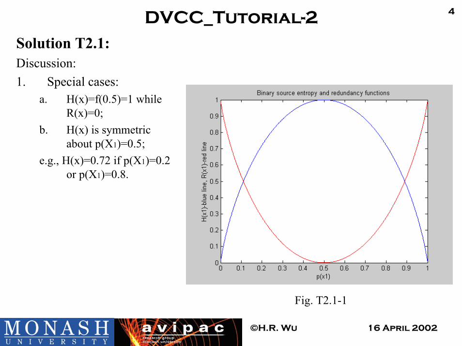
4DVCC_Tutorial-2Solution T2.1:Discussion:1. Special cases:
a. H(x)=f(0.5)=1 while R(x)=0;
b. H(x) is symmetric about p(X1)=0.5;
e.g., H(x)=0.72 if p(X1)=0.2 or p(X1)=0.8.
Fig. T2.1-1
16 April 2002©H.R. Wu
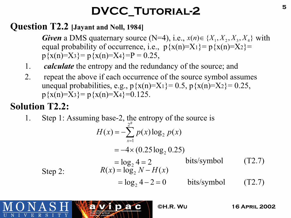
5DVCC_Tutorial-2Question T2.2 [Jayant and Noll, 1984]
Given a DMS quaternary source (N=4), i.e., with equal probability of occurrence, i.e., p{x(n)=X1}= p{x(n)=X2}= p{x(n)=X3}= p{x(n)=X4}=P = 0.25,
1. calculate the entropy and the redundancy of the source; and2. repeat the above if each occurrence of the source symbol assumes
unequal probabilities, e.g., p{x(n)=X1}= 0.5, p{x(n)=X2}= 0.25, p{x(n)=X3}= p{x(n)=X4}=0.125.
Solution T2.2:1. Step 1: Assuming base-2, the entropy of the source is
bits/symbol (T2.7)Step 2:
bits/symbol (T2.7)
1 2 3 4( ) { , , , }x n X X X X∈
2
21
2
2
( ) ( ) log ( )
4 (0.25log 0.25)log 4 2
B
xH x p x p x
=
= −
= − ×= =
∑
2
2
( ) log ( )log 4 2 0
R x N H x= −= − =

16 April 2002©H.R. Wu
6DVCC_Tutorial-2Question T2.2 [Jayant and Noll, 1984]
Solution T2.2:1. Step 1: Assuming base-2, the entropy of the source is
bits/symbol (T2.7)Step 2:
bits/symbol (T2.7)
( )
2
21
2 2 2
( ) ( ) log ( )
0.5log 0.5 0.25log 0.25 0.125log 0.1251.75
B
xH x p x p x
=
= −
= − + +
=
∑
2
2
( ) log ( )log 4 1.750.25
R x N H x= −= −=
16 April 2002©H.R. Wu
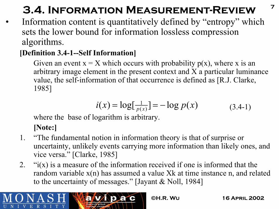
73.4. Information Measurement-Review• Information content is quantitatively defined by “entropy” which
sets the lower bound for information lossless compression algorithms.
[Definition 3.4-1--Self Information]Given an event x = X which occurs with probability p(x), where x is an arbitrary image element in the present context and X a particular luminance value, the self-information of that occurrence is defined as [R.J. Clarke, 1985]
(3.4-1)where the base of logarithm is arbitrary.[Note:]
1. “The fundamental notion in information theory is that of surprise or uncertainty, unlikely events carrying more information than likely ones, and vice versa.” [Clarke, 1985]
2. “i(x) is a measure of the information received if one is informed that the random variable x(n) has assumed a value Xk at time instance n, and related to the uncertainty of messages.” [Jayant & Noll, 1984]
1( )( ) log[ ] log ( )p xi x p x= = −

16 April 2002©H.R. Wu
83.4. Information Measurement-Review[Definition 3.4-2--Entropy]
Given an event x = X which occurs with probability p(x), where x is an arbitrary image element in the present context and X a particular luminance value, the average value of self-information per picture element over the whole image is termed (zeroth-order) entropy of the image array and defined as [R.J. Clarke, 1985; N. Jayant and P. Noll, 1984]
(3.4-3)where the base 2 is assumed for the logarithm operation.
[NOTE:]1. H(x) is the average information received if one is informed about the value
the random variable x(n) has assumed at time instance n.2. (3.4-4)
where left-side equality holds if all value probabilities except one are zero and therefore the only non-zero probability is unity, implying a totally predicable source; and the right hand side equality holds if and only if all probabilities are equal, describing the most unpredictable source.
2 2
21 1
( ) ( ) ( ) ( ) log ( )B B
x x
H x p x i x p x p x= =
= = −∑ ∑
20 ( ) logH x N≤ ≤

16 April 2002©H.R. Wu
93.4. Information Measurement-Review[Definition 3.4-3—Redundancy of the source]
Given an event x = X which occurs with probability p(x), where x is an arbitrary image element in the present context and X a particular luminance value which is one of the N values of a source set, the quantity log2N is the maximum value of the entropy of the source, also known as the capacity of the set. The redundancy R(x) of the source is defined as the difference between the capacity and the entropy: [N. Jayant and P. Noll, 1984]
(3.4-5)2( ) log ( )R x N H x= −where the base 2 is assumed for the logarithm operation.
16 April 2002©H.R. Wu
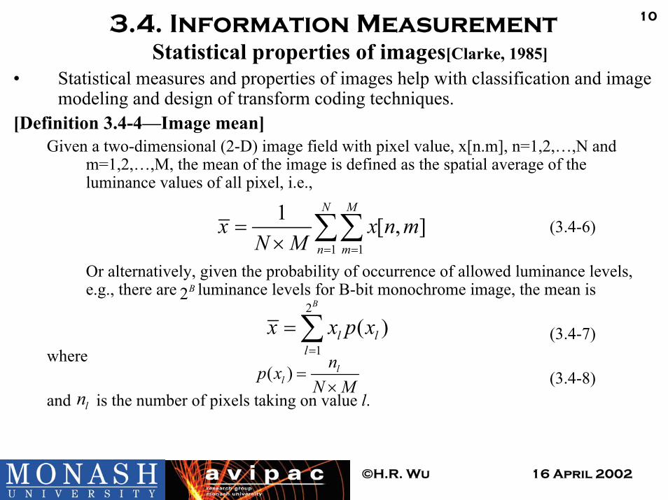
103.4. Information MeasurementStatistical properties of images[Clarke, 1985]
• Statistical measures and properties of images help with classification and image modeling and design of transform coding techniques.
[Definition 3.4-4—Image mean]Given a two-dimensional (2-D) image field with pixel value, x[n.m], n=1,2,…,N and
m=1,2,…,M, the mean of the image is defined as the spatial average of the luminance values of all pixel, i.e.,
(3.4-6)
Or alternatively, given the probability of occurrence of allowed luminance levels, e.g., there are luminance levels for B-bit monochrome image, the mean is
(3.4-7)where
(3.4-8)and is the number of pixels taking on value l.
1 1
1 [ , ]N M
n mx x n m
N M = =
=× ∑∑
2B
2
1
( )B
l ll
x x p x=
= ∑( ) l
lnp x
N M=
×ln

16 April 2002©H.R. Wu
113.4. Information MeasurementStatistical properties of images[Clarke, 1985]
[Definition 3.4-5—Image variance]Given a two-dimensional (2-D) image field with pixel value, x[n.m], n=1,2,…,N and m=1,2,…,M, the variance of the image is defined as the average value of the squared difference between the value of an arbitrary pixel and the image mean, i.e.,
(3.4-9) Or alternatively, given the probability of occurrence of allowed luminance levels, e.g., there are luminance levels for B-bit monochrome image, the mean is
(3.4-10)where
(3.4-11)and is the number of pixels taking on value l and .[NOTE:] 1. The square root of the variance is the standard deviation.
2B
22 2
1( ) ( )
B
l ll
x x p xσ=
= −∑( ) l
lnp x
N M=
×ln
2 2
1 1
1 ( [ , ] )N M
n mx n m x
N Mσ
= =
= −× ∑∑
0 2Bl≤ <
16 April 2002©H.R. Wu
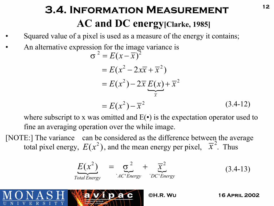
123.4. Information MeasurementAC and DC energy[Clarke, 1985]
• Squared value of a pixel is used as a measure of the energy it contains;• An alternative expression for the image variance is
(3.4-12)
where subscript to x was omitted and E(•) is the expectation operator used to fine an averaging operation over the while image.
[NOTE:] The variance can be considered as the difference between the average total pixel energy, , and the mean energy per pixel, . Thus
(3.4-13)
2 2
2 2
2 2
2 2
( )( 2 )( ) 2 ( )
( )x
E x xE x xx xE x x E x x
E x x
σ = −
= − +
= − +
= −
2( )E x 2x
2 2 2
` ' ` '
( )AC Energy DC EnergyTotal Energy
E x xσ= +
16 April 2002©H.R. Wu
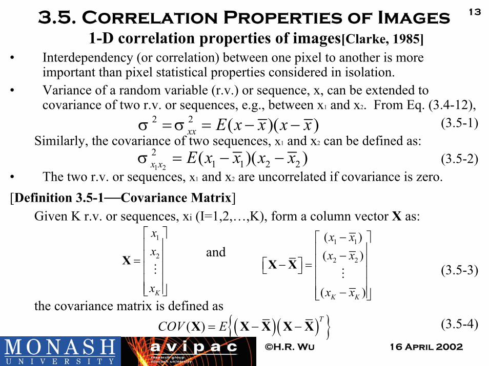
133.5. Correlation Properties of Images1-D correlation properties of images[Clarke, 1985]
• Interdependency (or correlation) between one pixel to another is more important than pixel statistical properties considered in isolation.
• Variance of a random variable (r.v.) or sequence, x, can be extended to covariance of two r.v. or sequences, e.g., between x1 and x2. From Eq. (3.4-12),
(3.5-1)Similarly, the covariance of two sequences, x1 and x2 can be defined as:
(3.5-2)• The two r.v. or sequences, x1 and x2 are uncorrelated if covariance is zero.[Definition 3.5-1—Covariance Matrix]
Given K r.v. or sequences, xi (I=1,2,…,K), form a column vector X as:
and (3.5-3)
the covariance matrix is defined as (3.5-4)
2 2 ( )( )xx E x x x xσ σ= = − −
1 2
21 1 2 2( )( )x x E x x x xσ = − −
1
2
K
xx
x
=
X
1 1
2 2
( )( )
( )K K
x xx x
x x
− − − = −
X X
( )( ){ }( )T
COV E= − −X X X X X
16 April 2002©H.R. Wu
143.5. Correlation Properties of Images1-D correlation properties of images[Clarke, 1985]
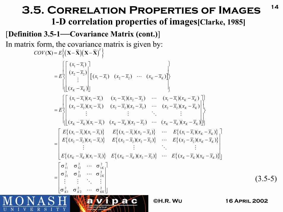
[Definition 3.5-1—Covariance Matrix (cont.)]In matrix form, the covariance matrix is given by:
(3.5-5)
( )( ){ }
[ ]1 1
2 21 1 2 2
1 1 1 1 1 1 2 2 1 1
2 2 1 1 2 2 2 2 2 2
1 1
( )
( )( )
( ) ( ) ( )
( )
( )( ) ( )( ) ( )( )( )( ) ( )( ) ( )( )
( )( ) (
T
K K
K K
K K
K K
K K K
COV E
x xx x
E x x x x x x
x x
x x x x x x x x x x x xx x x x x x x x x x x x
E
x x x x x x
= − −
− − = − − − −
− − − − − −− − − − − −
=
− − −
X X X X X
{ } { } { }{ } { } { }
{ } { } { }
2 2
1 1 1 1 1 1 2 2 1 1
2 2 1 1 2 2 2 2 2 2
1 1 2 2
)( ) ( )( )
( )( ) ( )( ) ( )( )( )( ) ( )( ) ( )( )
( )( ) ( )( ) ( )( )
K K K K K
K K
K K
K K K K K K K K
x x x x x x
E x x x x E x x x x E x x x xE x x x x E x x x x E x x x x
E x x x x E x x x x E x x x x
− − −
− − − − − − − − − − − −=
− − − − − −2 2 211 12 12 2 221 22 2
2 2 21 2
K
K
K K KK
σ σ σσ σ σ
σ σ σ
=
16 April 2002©H.R. Wu
153.5. Correlation Properties of Images1-D correlation properties of images[Clarke, 1985]
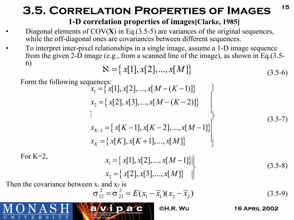
• Diagonal elements of COV(X) in Eq.(3.5-5) are variances of the original sequences, while the off-diagonal ones are covariances between different sequences.
• To interpret inter-pixel relationships in a single image, assume a 1-D image sequence from the given 2-D image (e.g., from a scanned line of the image), as shown in Eq.(3.5-6)
(3.5-6)Form the following sequences:
(3.5-7)
For K=2,(3.5-8)
Then the covariance between x1 and x2 is(3.5-9)
{ }[1], [2],..., [ ]x x x Mℵ=
{ }{ }
{ }{ }
1
2
1
[1], [2],..., [ ( 1)]
[2], [3],..., [ ( 2)]
[ 1], [ 2],..., [ 1]
[ ], [ 1],..., [ ]K
K
x x x x M K
x x x x M K
x x K x K x M
x x K x K x M−
= − −
= − − = − − − = +
{ }{ }
1
2
[1], [2],..., [ 1]
[2], [3],..., [ ]
x x x x M
x x x x M
= −
=
2 212 21 1 1 2 2( )( )E x x x xσ σ= = − −
16 April 2002©H.R. Wu
163.5. Correlation Properties of Images1-D correlation properties of images[Clarke, 1985]
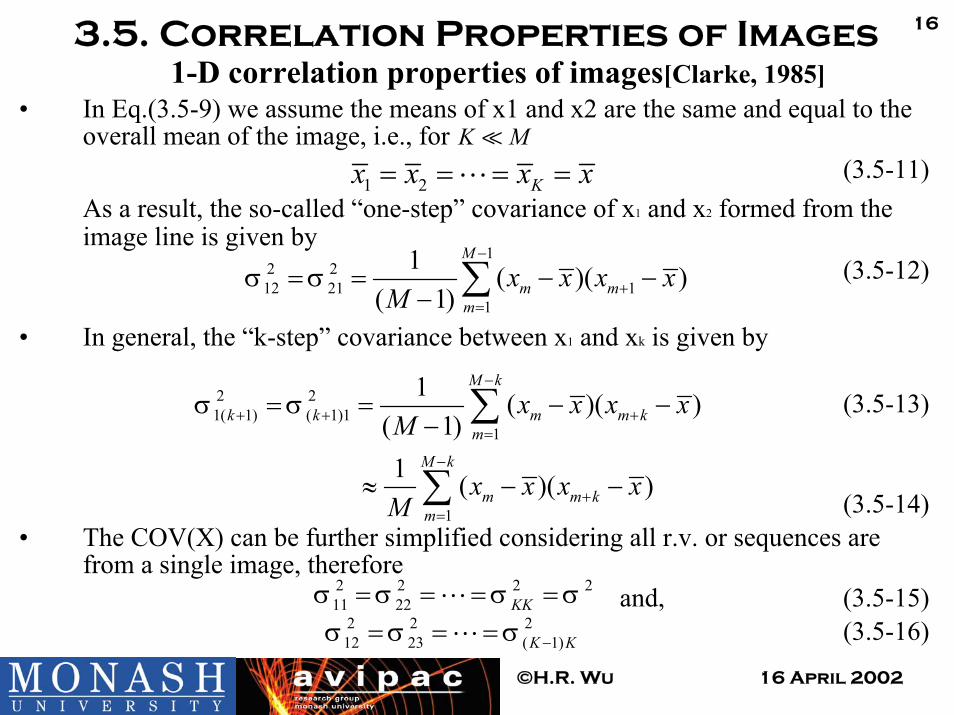
• In Eq.(3.5-9) we assume the means of x1 and x2 are the same and equal to the overall mean of the image, i.e., for
(3.5-11)As a result, the so-called “one-step” covariance of x1 and x2 formed from the image line is given by
(3.5-12)
• In general, the “k-step” covariance between x1 and xk is given by
(3.5-13)
(3.5-14)• The COV(X) can be further simplified considering all r.v. or sequences are
from a single image, therefore and, (3.5-15)
(3.5-16)
1 2 Kx x x x= = = =
12 212 21 1
1
1 ( )( )( 1)
M
m mm
x x x xM
σ σ−
+=
= = − −− ∑
K M
2 21( 1) ( 1)1
1
1
1 ( )( )( 1)1 ( )( )
M k
k k m m km
M k
m m km
x x x xM
x x x xM
σ σ−
+ + +=
−
+=
= = − −−
≈ − −
∑
∑
2 2 212 23 ( 1)K Kσ σ σ −= = =
2 2 2 211 22 KKσ σ σ σ= = = =

16 April 2002©H.R. Wu
173.5. Correlation Properties of Images1-D correlation properties of images[Clarke, 1985]
• Considering Eqs.(3.5-15 & 16),
(3.5-17)
Note that (3.5-16)
• Dividing all elements in COV(X) gives the correlation or normalized covariance matrix:
(3.5-17)
where (3.5-18)
2 2ij jiσ σ=
2 2 21 1
2 2 21 2
2 2 21 2
( )
K
K
K K
COV
σ σ σσ σ σ
σ σ σ
−
−
− −
=
X
1 1
1 2
1 2
11
( )
1
K
K
K K
COR
ρ ρρ ρ
ρ ρ
−
−
− −
=
X
2
1, 0
1,2,... .k k
if k
if k Kρ σ
σ
==
=
16 April 2002©H.R. Wu
183.5. Correlation Properties of Images1-D correlation properties of images[Clarke, 1985]
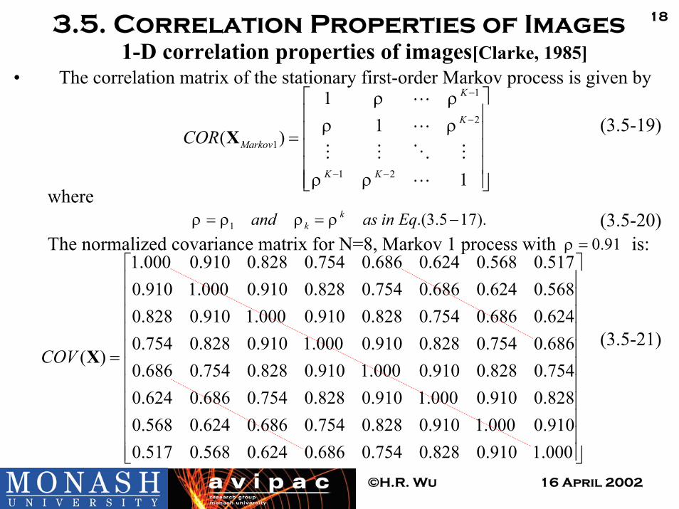
• The correlation matrix of the stationary first-order Markov process is given by
(3.5-19)
where (3.5-20)
The normalized covariance matrix for N=8, Markov 1 process with is:
(3.5-21)
1
2
1
1 2
11
( )
1
K
K
Markov
K K
COR
ρ ρρ ρ
ρ ρ
−
−
− −
=
X
1 .(3.5 17).kkand as in Eqρ ρ ρ ρ= = −
0.91ρ =1.000 0.910 0.828 0.754 0.686 0.624 0.568 0.5170.910 1.000 0.910 0.828 0.754 0.686 0.624 0.5680.828 0.910 1.000 0.910 0.828 0.754 0.686 0.6240.754 0.828 0.910 1.000 0.910 0.828 0.754 0.686
( )0.686 0.754 0.828 0.910 1.000 0.910 0.8
COV =X28 0.754
0.624 0.686 0.754 0.828 0.910 1.000 0.910 0.8280.568 0.624 0.686 0.754 0.828 0.910 1.000 0.9100.517 0.568 0.624 0.686 0.754 0.828 0.910 1.000

16 April 2002©H.R. Wu
19DVCC_Tutorial-2Demonstration T2.1—Having fun with Matlab
Picture of Claude E. Shannon

16 April 2002©H.R. Wu
20Demonstration T2.1—Having fun with MatlabShannon Image
H(x)=7.3020Or R(x)=8-7.3020=0.6980Mean=126.0862Variance=4,518.
H(x)=4.1249Or R(x)=8-4.1249=3.8751Mean=0.0107Variance=65.8942