screening methods in sensitivity analysis · the setup for sensitivity analysis of simulation...

Screening methods in sensitivity analysis

M. Ratto

Ispra, Nov 2017

1

2

Screening methods

The setup for sensitivity analysis of simulation results is similar to that of physical experimentation but…

Screening designs can be considered asthe development of Design of Experiments (DOE)

DOE determines how much the variables involved in a physical experiment affect one or more measurements

3

Screening methods

…. simulations allows to explore more complex system with many more variables

screening designs

able to “screen” a subset of few important input variables among the many (hundreds, thousands) often contained in models

Goal: Model simplification / Model lumping / Pre-calibration

4

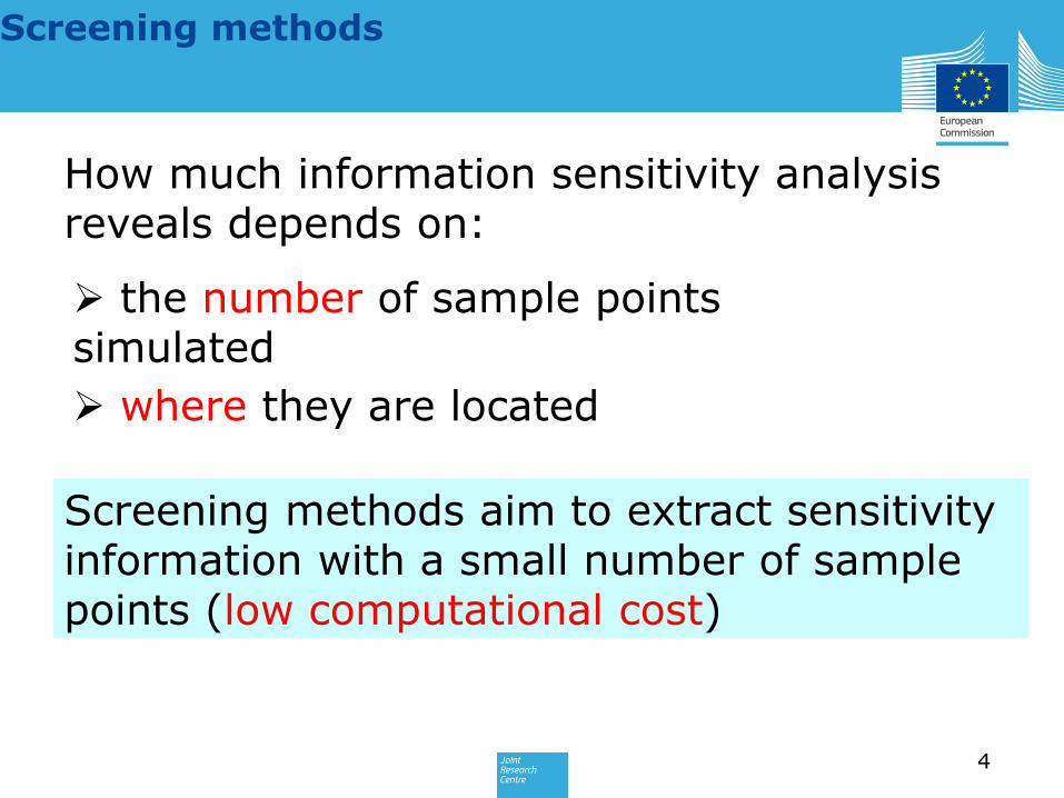
Screening methods

How much information sensitivity analysis reveals depends on:

Screening methods aim to extract sensitivity information with a small number of sample points (low computational cost)

the number of sample points simulated

where they are located

November 20, 2017

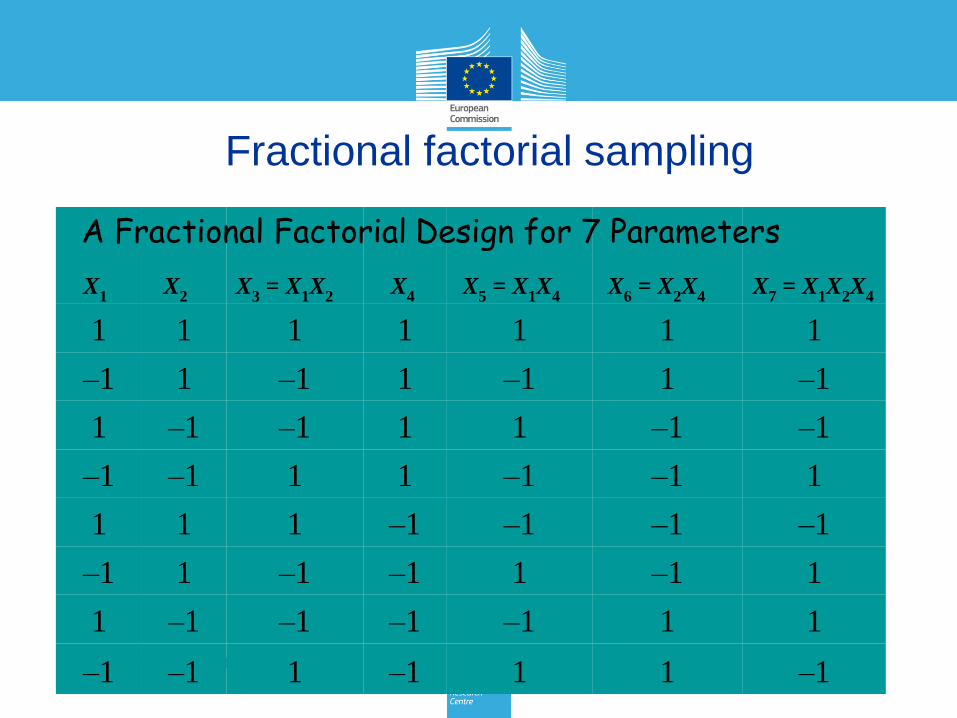
Fractional factorial sampling

A 2-Level Full Factorial Design for 3 parameters

X1 X2 X3

1 1 1

–1 1 1

1 –1 1

–1 –1 1

1 1 –1

–1 1 –1

1 –1 –1

–1 –1 –1

The Full Factorial Design

November 20, 2017


A disadvantage of a factorial design is the enormous number of simulations required

Using 2 levels: 10 parameters 210 = 1024 simulations

20 parameters more than a million!!

SolutionTo select only a fraction of these simulations to generate a smaller design that can still produce valuable results

November 20, 2017 7

X1

X2

X3

= X1X

2X

4 X

5= X

1X

4X

6= X

2X

4X

7= X

1X

2X

4

1 1 1 1 1 1 1

–1 1 –1 1 –1 1 –1

1 –1 –1 1 1 –1 –1

–1 –1 1 1 –1 –1 1

1 1 1 –1 –1 –1 –1

–1 1 –1 –1 1 –1 1

1 –1 –1 –1 –1 1 1

–1 –1 1 –1 1 1 –1


A Fractional Factorial Design for 7 Parameters

8

The method of Elementary Effects

The EE method can be seen as an extension of a derivative-based analysis

local measure

small perturbation around base values

Problems related to a derivative-based approach:

Derivative = 0 only implies that a factor is locally non influent

(Morris, 1991)

9

Example

12

2 1* * 1 4 *4

πy x x

Derivatives

1 2

1 2

1 0

2 0

0

4

x x

x x

y

x

y

x π

10


Model 1( ,.., )ky y x x

Elementary Effect for the ith input factor in a point Xo

1 2 1 1 1

1

0 0 0 0 0 0 0 0,

0 0( , ,.., Δ, ,.., ) ( ,..., )

( ,..., )Δ

i i i k k

ki

y x x x x x x y x xEE x x

(Morris, 1991)

is larger than

in local methods

x1

x2

(x01, x0

2) (x01+, x0

2)

Each input varies across l possible values (levels) within its range of variation

Distribution not uniform levels correspond to distribution quantiles

xi U(0,1) l = 4 l1 = 0 l2 = 1/3 l3 = 2/3 l4 = 1


The value of (sampling step) is a function of l

Optimal choice for is = l / 2 (l -1)

November 20, 2017


0 1/3 2/3 10 1/3 2/3 1

13


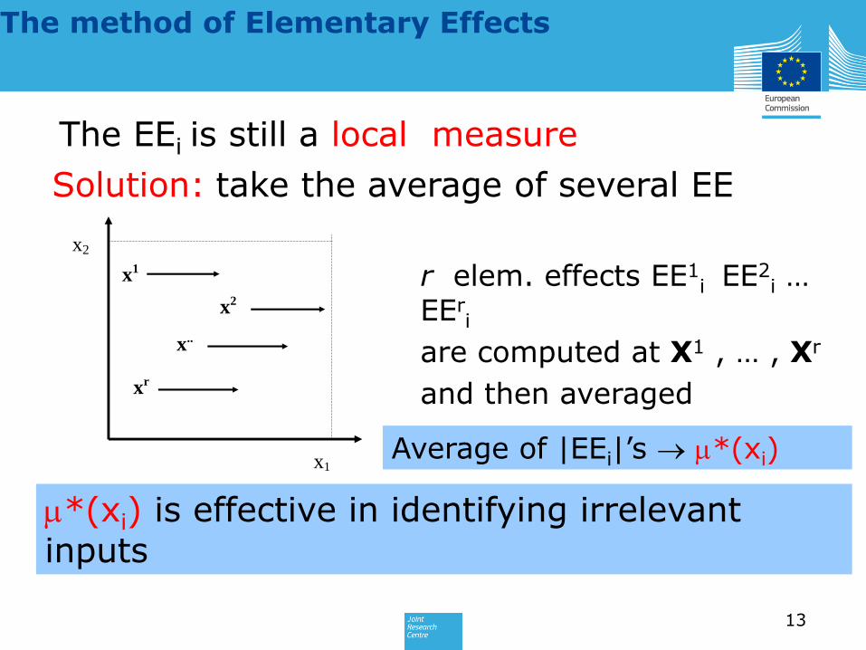
The EEi is still a local measure

Solution: take the average of several EE

x1

x2

x1

x2

x..

xr

r elem. effects EE1i EE2

i … EEr

i

are computed at X1 , … , Xr

and then averaged

Average of |EEi|’s *(xi)

*(xi) is effective in identifying irrelevant inputs

14

Implementing the EE method

Morris builds r trajectories of (k+1) sample points each providing one EE per input

Goal: estimate r EE’s per input

(Morris, 1991)

x1

x2

x3

Y1 Y

2

Y3

Y4

A trajectory of the EE design

EE11 = (Y2- Y1) /

EE12 = (Y3- Y2) /

EE13 = (Y4- Y3) /

Total cost = r (k + 1)r is in the range 4 -20

15November 20, 2017

The example

12

2 1* * 1 4 *4

πy x x

EE (l=4, r=10)

1

2

*( ) 0.070

*( ) 0.024

μ x

μ x

Derivatives

1 2

4(0,0) 0 (0,0)

y y

x x π

November 20, 2017

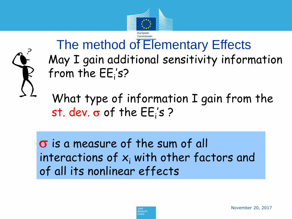
is a measure of the sum of all interactions of xi with other factors and of all its nonlinear effects

What type of information I gain from the st. dev. of the EEi’s ?

May I gain additional sensitivity information from the EEi’s?


November 20, 2017http://www.jrc.cec.eu.int/uasa

17

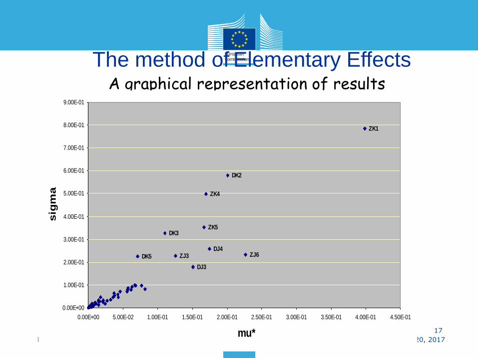
A graphical representation of results

ZK1

ZJ6

DK2

DJ4

ZK4

ZK5

DJ3

DK3

ZJ3DK5

0.00E+00

1.00E-01

2.00E-01

3.00E-01

4.00E-01

5.00E-01

6.00E-01

7.00E-01

8.00E-01

9.00E-01

0.00E+00 5.00E-02 1.00E-01 1.50E-01 2.00E-01 2.50E-01 3.00E-01 3.50E-01 4.00E-01 4.50E-01

mu*

sig

ma


November 20, 2017

An analytical example (Morris, 1991)

ljilji

ljijiji

jiii

i wwwwwwy

10

,,

10

,

20

10

w1, w2,..., w10 in [-1,1]

Other coefficients ~ N(0,1)

βi = -15; i = 1, 2

βi,j = 30; i, j = 3, 4

βi,j,l = 10; i, j, l = 1,…,4wi = 2 (xi – 0.5) for i ≠ 3

w3 = 2 (1.1x3 / (x3 + 0. 1)- 0.5)

xi ~ U[0; 1]

November 20, 2017

An analytical example

00000000

5

1

7,8,9,10

2

3

4

611,…20

0

5

10

15

20

25

30

0 10 20 30 40 50

Mu*

Sig

ma

r =4

l =4

= 2/3

November 20, 2017

0

5

10

15

20

25

30

35

40

45

50

0 10 20 30 40 50 60

mustar

sig

ma

0

10

20

30

40

50

60

0 20 40 60

mustar

sig

ma

0

5

10

15

20

25

30

35

40

45

0 10 20 30 40 50 60 70

mustar

sig

ma

0

10

20

30

40

50

60

0 10 20 30 40 50

mustar

sig

ma

“missed” factors, r=4

November 20, 2017 21

Test case 3

,

0

1

2

3

4

5

6

7

8

9

0 2 4 6 80

2

4

6

8

10

12

0 2 4 6 8 10

0

2

4

6

8

10

12

0 2 4 6 8 10

0

2

4

6

8

10

12

0 2 4 6 8 10

0

2

4

6

8

10

12

14

0 2 4 6 8 10 12

0

2

4

6

8

10

12

14

0 2 4 6 8 10 12

22

Identification ??

Ex-ante identification screening …

Lacks the collinearity component (only sensitivity effect).

Potential for very expensive ABM models ?

23

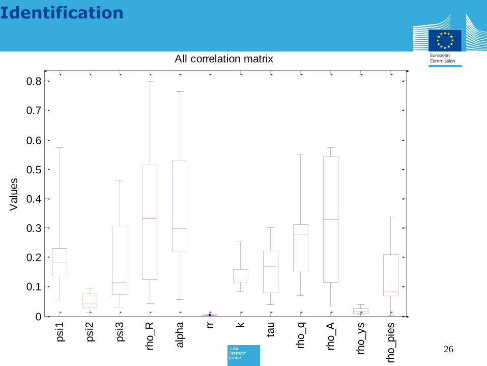
Identification

Covariance/autocovariance matrices among observed variables yt:

corr(yt); corr(yt, yt-k);

[nobs x (nobs-1)/2];

[nobs x nobs]

24

Identification

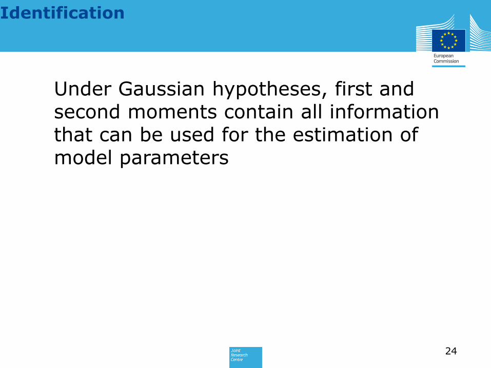
Under Gaussian hypotheses, first and second moments contain all information that can be used for the estimation of model parameters

25

Identification

0

10

20

30

40

50

60

70

80

Valu

es

psi1

psi2

psi3

rho_R

alp

ha rr k

tau

rho_q

rho_A

rho_ys

rho_pie

s

All variance decomposition

26

Identification

0

0.1

0.2

0.3

0.4

0.5

0.6

0.7

0.8

Valu

es

psi1

psi2

psi3

rho_R

alp

ha rr k

tau

rho_q

rho_A

rho_ys

rho_pie

s

All correlation matrix

27

Identification

0

0.1

0.2

0.3

0.4

0.5

0.6

0.7

0.8

0.9

Valu

es

psi1

psi2

psi3

rho_R

alp

ha rr k

tau

rho_q

rho_A

rho_ys

rho_pie

s

All autocorrelation

Often they rely on the assumption that the number of important parameters is small

Screening designs are useful to “screen” a subset of few important input variables among the many contained in models

Their feature is the low computational cost (low number of model evaluations)

28

Conclusions

29

Conclusions

Quick screening tests for ex-ante identification (sensitivity component) of DSGE models

30

Mapping the reduced form of RE models

Relationship between the reduced form of a rational expectation model and the structural coefficients.

let the reduced form beyt=Tyt-1+But,

'outputs' Y of our analysis will be theentries in the transition matrix T(X1,…,Xk) or in thematrix B(X1,…,Xk).

31

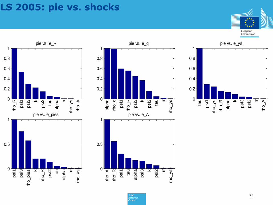
LS 2005: pie vs. shocks

0

0.2

0.4

0.6

0.8

1

rho_R

psi1

psi3 k

psi2

tau

alp

ha rr

rho_ys

rho_A

pie vs. e_R

0

0.2

0.4

0.6

0.8

1

alp

ha

rho_q

psi1

rho_R

psi3 k

psi2

tau rr

rho_ys

pie vs. e_q

0

0.2

0.4

0.6

0.8

1

tau

psi1

rho_ys

rho_R

alp

ha k

psi3

psi2 rr

rho_A

pie vs. e_ys

0

0.5

1

psi1

psi3

rho_pie

s k

rho_R

psi2

tau

alp

ha rr

rho_ys

pie vs. e_pies

0

0.5

1

rho_A

rho_R

psi1

tau

alp

ha

psi3 k

psi2 rr

rho_ys

pie vs. e_A

32

LS 2005: pie vs. lags

0

0.2

0.4

0.6

0.8

1

tau

rho_R

rho_ys

alp

ha

psi1 k

psi3

psi2 rr

rho_A

R vs. y_s(-1)

0

0.2

0.4

0.6

0.8

1

rho_R k

psi1

psi3

psi2

alp

ha

tau rr

rho_ys

rho_A

R vs. R(-1)

0

0.2

0.4

0.6

0.8

1

rho_q

alp

ha

rho_R

psi1 k

psi3

psi2

tau rr

rho_ys

R vs. dq(-1)

0

0.5

1

rho_pie

s

psi1

psi3

rho_R k

psi2

tau rr

alp

ha

rho_ys

R vs. pie_s(-1)

0

0.5

1

rho_A

rho_R

tau

alp

ha

psi1 k

psi3

psi2 rr

rho_ys

R vs. A(-1)

0

0.1

0.2

0.3

0.4

0.5

0.6

0.7

0.8

0.9

1

Ele

menta

ry E

ffects

psi1

psi2

psi3

rho_R

alp

ha rr k

tau

rho_q

rho_A

rho_ys

rho_pie

s

Reduced form screening

33

LS 2005: overall picture

34

References

Campolongo F., Cariboni J., Saltelli A., 2006, An effective screening design for sensitivity analysis of large models, under revisions.

Saltelli, A., Tarantola, S., Campolongo, F., and Ratto, M., 2005, Sensitivity Analysis for Chemical Models, Chemical Reviews, 105(7), pp 2811 - 2828

Saltelli, A., Tarantola, S., Campolongo, F., and Ratto, M., 2004, Sensitivity Analysis in Practice. A Guide to Assessing Scientific Models, John Wiley & Sons publishers, Probability and Statistics series

Saltelli A., Chan K., Scott E.M., 2000, Sensitivity Analysis, John Wiley & Sons publishers, Probability and Statistics series, 355-365

Morris M. D., 1991, Factorial sampling plans for preliminary computational experiments, Technometrics, 33(2): 161-174

screening methods in sensitivity analysis · the setup for sensitivity analysis of simulation...

Documents