sdt primer - sdtools

Structural Dynamics Toolbox Primer

SDTools

REVISED FOR SDT 6.2Originally by : Prof N.A.J. Lieven, University of Bristol

Jean Philippe Bianchi, Etienne Balmes

September 11, 2013

Contents

1 Finite element modeling 5

1.1 SDT Basics and concepts . . . . . . . . . . . . . . . . . . . . . . . . . . . . . . . . . . . . 6

1.1.1 Functions and commands . . . . . . . . . . . . . . . . . . . . . . . . . . . . . . . . 6

1.1.2 Conventions in manual . . . . . . . . . . . . . . . . . . . . . . . . . . . . . . . . . . 6

1.1.3 Data structures and stacks . . . . . . . . . . . . . . . . . . . . . . . . . . . . . . . 7

1.1.4 SDT pointer strategies . . . . . . . . . . . . . . . . . . . . . . . . . . . . . . . . . . 7

1.2 FEM model . . . . . . . . . . . . . . . . . . . . . . . . . . . . . . . . . . . . . . . . . . . . 7

1.2.1 FEM model data structure . . . . . . . . . . . . . . . . . . . . . . . . . . . . . . . 7

1.2.2 Viewing model with feplot . . . . . . . . . . . . . . . . . . . . . . . . . . . . . . . 8

1.2.3 Controlling views, node and element selection . . . . . . . . . . . . . . . . . . . . . 10

1.2.4 Viewing deformations . . . . . . . . . . . . . . . . . . . . . . . . . . . . . . . . . . 10

1.3 Meshing and model manipulations . . . . . . . . . . . . . . . . . . . . . . . . . . . . . . . 10

1.3.1 Explicit definition . . . . . . . . . . . . . . . . . . . . . . . . . . . . . . . . . . . . 11

1.3.2 Functional definition of meshes . . . . . . . . . . . . . . . . . . . . . . . . . . . . . 12

1.3.3 Automated (free) meshing from geometry (CAD) . . . . . . . . . . . . . . . . . . . 16

1.4 Elements . . . . . . . . . . . . . . . . . . . . . . . . . . . . . . . . . . . . . . . . . . . . . 17

1.4.1 Model description matrix . . . . . . . . . . . . . . . . . . . . . . . . . . . . . . . . 17

1.4.2 Element topologies and problem formulations . . . . . . . . . . . . . . . . . . . . . 18

1.4.3 Identifier manipulations in element definitions . . . . . . . . . . . . . . . . . . . . . 18

1.5 Material and element properties . . . . . . . . . . . . . . . . . . . . . . . . . . . . . . . . . 19

1.5.1 Material Properties . . . . . . . . . . . . . . . . . . . . . . . . . . . . . . . . . . . . 19

1.5.2 Section Properties . . . . . . . . . . . . . . . . . . . . . . . . . . . . . . . . . . . . 20

1.6 Loads and boundary conditions . . . . . . . . . . . . . . . . . . . . . . . . . . . . . . . . . 21

1.6.1 Degrees of freedom . . . . . . . . . . . . . . . . . . . . . . . . . . . . . . . . . . . . 21

1.6.2 Fixed boundary conditions . . . . . . . . . . . . . . . . . . . . . . . . . . . . . . . 22

1.6.3 Loads . . . . . . . . . . . . . . . . . . . . . . . . . . . . . . . . . . . . . . . . . . . 22

1.7 Solving . . . . . . . . . . . . . . . . . . . . . . . . . . . . . . . . . . . . . . . . . . . . . . . 22

1.7.1 fe simul generic integrated solver . . . . . . . . . . . . . . . . . . . . . . . . . . . 23

1.7.2 fe eig real eigenvalue solution . . . . . . . . . . . . . . . . . . . . . . . . . . . . . 23

1.7.3 fe time full model transient and NL analysis . . . . . . . . . . . . . . . . . . . . . 23

1.7.4 nor2xf, modal frequency response . . . . . . . . . . . . . . . . . . . . . . . . . . . 24

1.8 Post-processing . . . . . . . . . . . . . . . . . . . . . . . . . . . . . . . . . . . . . . . . . . 24

1.8.1 feplot . . . . . . . . . . . . . . . . . . . . . . . . . . . . . . . . . . . . . . . . . . 25

1.8.2 iiplot . . . . . . . . . . . . . . . . . . . . . . . . . . . . . . . . . . . . . . . . . . 25

1.9 A complete example . . . . . . . . . . . . . . . . . . . . . . . . . . . . . . . . . . . . . . . 26

3

4 CONTENTS

2 Experimental modal analysis 292.1 Testing . . . . . . . . . . . . . . . . . . . . . . . . . . . . . . . . . . . . . . . . . . . . . . 30

2.1.1 Measuring transfer functions . . . . . . . . . . . . . . . . . . . . . . . . . . . . . . 302.1.2 Multiple locations to get shapes . . . . . . . . . . . . . . . . . . . . . . . . . . . . . 31

2.2 Identification (mode extraction) . . . . . . . . . . . . . . . . . . . . . . . . . . . . . . . . . 312.2.1 Importing measurements into iiplot, idcom . . . . . . . . . . . . . . . . . . . . . . 312.2.2 Identified modal model . . . . . . . . . . . . . . . . . . . . . . . . . . . . . . . . . 332.2.3 Single mode peak picking method . . . . . . . . . . . . . . . . . . . . . . . . . . . 332.2.4 Multi-mode estimation and refinement method . . . . . . . . . . . . . . . . . . . . 34

2.3 Test geometry and visualization . . . . . . . . . . . . . . . . . . . . . . . . . . . . . . . . . 342.3.1 Wire frame model . . . . . . . . . . . . . . . . . . . . . . . . . . . . . . . . . . . . 342.3.2 Sensor placement . . . . . . . . . . . . . . . . . . . . . . . . . . . . . . . . . . . . . 362.3.3 Visualizing test shapes (ODS, modes, ...) . . . . . . . . . . . . . . . . . . . . . . . 38

2.4 A complete modal test example . . . . . . . . . . . . . . . . . . . . . . . . . . . . . . . . . 38

3 Correlation 413.1 Topology correlation . . . . . . . . . . . . . . . . . . . . . . . . . . . . . . . . . . . . . . . 423.2 Correlation criteria . . . . . . . . . . . . . . . . . . . . . . . . . . . . . . . . . . . . . . . . 42

3.2.1 Modal Assurance Criteria (MAC) . . . . . . . . . . . . . . . . . . . . . . . . . . . . 423.2.2 Auto MAC . . . . . . . . . . . . . . . . . . . . . . . . . . . . . . . . . . . . . . . . 433.2.3 Standard MAC . . . . . . . . . . . . . . . . . . . . . . . . . . . . . . . . . . . . . . 433.2.4 COMAC . . . . . . . . . . . . . . . . . . . . . . . . . . . . . . . . . . . . . . . . . . 433.2.5 eCOMAC . . . . . . . . . . . . . . . . . . . . . . . . . . . . . . . . . . . . . . . . . 44

3.3 Modeshape expansion . . . . . . . . . . . . . . . . . . . . . . . . . . . . . . . . . . . . . . 44

Bibliography 45

1

Finite element modeling

Contents

1.1 SDT Basics and concepts . . . . . . . . . . . . . . . . . . . . . . . . . . . . . . 6

1.1.1 Functions and commands . . . . . . . . . . . . . . . . . . . . . . . . . . . . . . 6

1.1.2 Conventions in manual . . . . . . . . . . . . . . . . . . . . . . . . . . . . . . . . 6

1.1.3 Data structures and stacks . . . . . . . . . . . . . . . . . . . . . . . . . . . . . 7

1.1.4 SDT pointer strategies . . . . . . . . . . . . . . . . . . . . . . . . . . . . . . . . 7

1.2 FEM model . . . . . . . . . . . . . . . . . . . . . . . . . . . . . . . . . . . . . . 7

1.2.1 FEM model data structure . . . . . . . . . . . . . . . . . . . . . . . . . . . . . 7

1.2.2 Viewing model with feplot . . . . . . . . . . . . . . . . . . . . . . . . . . . . . 8

1.2.3 Controlling views, node and element selection . . . . . . . . . . . . . . . . . . . 10

1.2.4 Viewing deformations . . . . . . . . . . . . . . . . . . . . . . . . . . . . . . . . 10

1.3 Meshing and model manipulations . . . . . . . . . . . . . . . . . . . . . . . . 10

1.3.1 Explicit definition . . . . . . . . . . . . . . . . . . . . . . . . . . . . . . . . . . 11

1.3.2 Functional definition of meshes . . . . . . . . . . . . . . . . . . . . . . . . . . . 12

1.3.3 Automated (free) meshing from geometry (CAD) . . . . . . . . . . . . . . . . . 16

1.4 Elements . . . . . . . . . . . . . . . . . . . . . . . . . . . . . . . . . . . . . . . . 17

1.4.1 Model description matrix . . . . . . . . . . . . . . . . . . . . . . . . . . . . . . 17

1.4.2 Element topologies and problem formulations . . . . . . . . . . . . . . . . . . . 18

1.4.3 Identifier manipulations in element definitions . . . . . . . . . . . . . . . . . . . 18

1.5 Material and element properties . . . . . . . . . . . . . . . . . . . . . . . . . 19

1.5.1 Material Properties . . . . . . . . . . . . . . . . . . . . . . . . . . . . . . . . . . 19

1.5.2 Section Properties . . . . . . . . . . . . . . . . . . . . . . . . . . . . . . . . . . 20

1.6 Loads and boundary conditions . . . . . . . . . . . . . . . . . . . . . . . . . . 21

1.6.1 Degrees of freedom . . . . . . . . . . . . . . . . . . . . . . . . . . . . . . . . . . 21

1.6.2 Fixed boundary conditions . . . . . . . . . . . . . . . . . . . . . . . . . . . . . 22

1.6.3 Loads . . . . . . . . . . . . . . . . . . . . . . . . . . . . . . . . . . . . . . . . . 22

1.7 Solving . . . . . . . . . . . . . . . . . . . . . . . . . . . . . . . . . . . . . . . . . 22

1.7.1 fe simul generic integrated solver . . . . . . . . . . . . . . . . . . . . . . . . . 23

1.7.2 fe eig real eigenvalue solution . . . . . . . . . . . . . . . . . . . . . . . . . . . 23

1.7.3 fe time full model transient and NL analysis . . . . . . . . . . . . . . . . . . . 23

1.7.4 nor2xf, modal frequency response . . . . . . . . . . . . . . . . . . . . . . . . . 24

1.8 Post-processing . . . . . . . . . . . . . . . . . . . . . . . . . . . . . . . . . . . . 24

1.8.1 feplot . . . . . . . . . . . . . . . . . . . . . . . . . . . . . . . . . . . . . . . . . 25

1.8.2 iiplot . . . . . . . . . . . . . . . . . . . . . . . . . . . . . . . . . . . . . . . . . 25

1.9 A complete example . . . . . . . . . . . . . . . . . . . . . . . . . . . . . . . . . 26

6 CHAPTER 1. FINITE ELEMENT MODELING

1.1 SDT Basics and concepts

1.1.1 Functions and commands

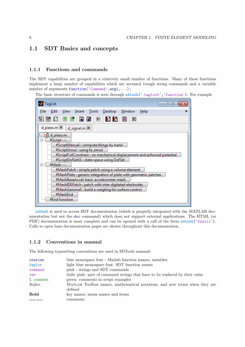
The SDT capabilities are grouped in a relatively small number of functions. Many of these functionsimplement a large number of capabilities which are accessed trough string commands and a variablenumber of arguments function(’Command’,arg1,...);

The basic structure of commands is seen through sdtweb(’ taglist’,’function’). For example

sdtweb is used to access SDT documentation (which is properly integrated with the MATLAB doc-umentation but not the doc command) which does not support external applications. The HTML (orPDF) documentation is most complete and can be opened with a call of the form sdtweb(’feutil’).Calls to open base documentation pages are shown throughout this documentation.

1.1.2 Conventions in manual

The following typesetting conventions are used in SDTools manuals

courier blue monospace font : Matlab function names, variablesfeplot light blue monospace font: SDT function namescommand pink : strings and SDT commandsvar italic pink: part of command strings that have to be replaced by their value% comment green: comments in script examplesItalics Matlab Toolbox names, mathematical notations, and new terms when they are

definedBold key names, menu names and itemsSmall print comments

1.2. FEM MODEL 7

1.1.3 Data structures and stacks

All data in SDT are stored in Matlab data structures. The basic structures are

• model FEM model, test wire frame, ... see sdtweb model

• def deformations (typical FEM output) see sdtweb def

• curve responses and general datasets ... see sdtweb curve

When extensible and possibly large lists of mixed data are needed, SDT uses .Stack fields which areN by 3 cell arrays with each row of the form {’type’,’name’,val}. The purpose of these cell arrays isto deal with unordered sets of data entries which can be classified by type and name.

stack get, stack set and stack rm commands are low level commands used to get/set/remove singleor multiple entries from stacks. iiplot and feplot implement easier named based indexing, see sdtweb

diiplot#CurveStack.

1.1.4 SDT pointer strategies

SDT pointer objects are

• sdth pointers to data contained in figures.Will be illustrated in section 1.2.2. In particular, theseare used to ease script base modification of feplot and iiplot figures.

• v handle implement pointers. Fundamental for handling of large data sets stored elsewhere (out-of-core file reading for example).

1.2 FEM model

1.2.1 FEM model data structure

The mesh generated during construction of an FE model is a mathematical representation of the struc-ture. FE packages allow definition of a geometry in the form of nodes, lines, surfaces which are used asa guide during meshing. There is a distinct difference between model geometry and the model mesh.

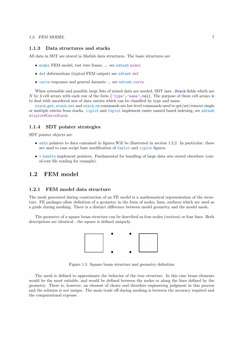
The geometry of a square beam structure can be described as four nodes (vertices) or four lines. Bothdescriptions are identical - the square is defined uniquely.

Figure 1.1: Square beam structure and geometry definition

The mesh is defined to approximate the behavior of the true structure. In this case beam elementswould be the most suitable, and would be defined between the nodes or along the lines defined by thegeometry. There is, however, an element of choice and therefore engineering judgment in this processand the solution is not unique. The main trade off during meshing is between the accuracy required andthe computational expense.


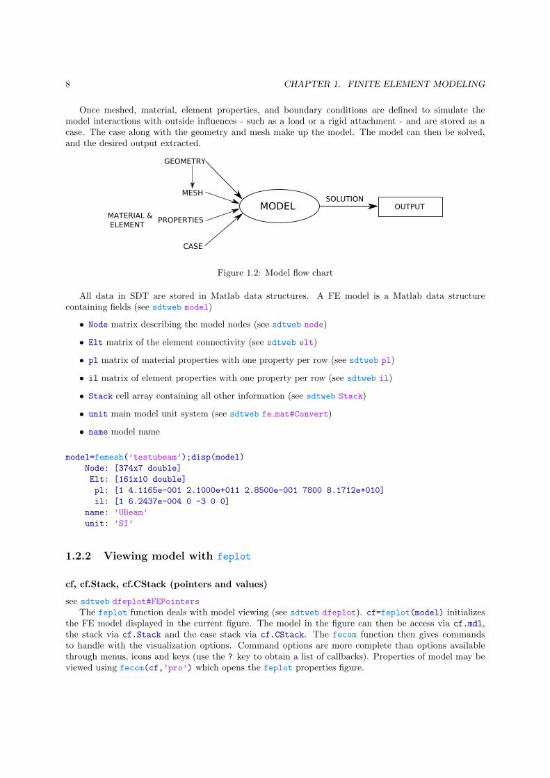
Once meshed, material, element properties, and boundary conditions are defined to simulate themodel interactions with outside influences - such as a load or a rigid attachment - and are stored as acase. The case along with the geometry and mesh make up the model. The model can then be solved,and the desired output extracted.

Figure 1.2: Model flow chart

All data in SDT are stored in Matlab data structures. A FE model is a Matlab data structurecontaining fields (see sdtweb model)

• Node matrix describing the model nodes (see sdtweb node)

• Elt matrix of the element connectivity (see sdtweb elt)

• pl matrix of material properties with one property per row (see sdtweb pl)

• il matrix of element properties with one property per row (see sdtweb il)

• Stack cell array containing all other information (see sdtweb Stack)

• unit main model unit system (see sdtweb fe mat#Convert)

• name model name

model=femesh(’testubeam’);disp(model)

Node: [374x7 double]

Elt: [161x10 double]

pl: [1 4.1165e-001 2.1000e+011 2.8500e-001 7800 8.1712e+010]

il: [1 6.2437e-004 0 -3 0 0]

name: ’UBeam’

unit: ’SI’

1.2.2 Viewing model with feplot

cf, cf.Stack, cf.CStack (pointers and values)

see sdtweb dfeplot#FEPointers

The feplot function deals with model viewing (see sdtweb dfeplot). cf=feplot(model) initializesthe FE model displayed in the current figure. The model in the figure can then be access via cf.mdl,the stack via cf.Stack and the case stack via cf.CStack. The fecom function then gives commandsto handle with the visualization options. Command options are more complete than options availablethrough menus, icons and keys (use the ? key to obtain a list of callbacks). Properties of model may beviewed using fecom(cf,’pro’) which opens the feplot properties figure.

1.2. FEM MODEL 9

% sdtweb demosdt(’DemoUbeam’)

model=demosdt(’demo ubeam mix NoPlot’);

cf=feplot(5); % empty model in figure 5

cf.model=model; % initialize model and display

fecom(’pro’); % display property figure

% You should analyze the tabs in the propery figure

• materials and element properties, sdtweb m elastic and sdtweb p solid calls.

• boundary conditions sdtweb fe case

• simul (standard solutions) sdtweb fe simul, sdtweb fe eig, sdtweb fe time.

For other interfaces see sdtweb femlink.

%% Output of commands above

>> cf=feplot

cf =

FEPLOT in figure 5

Selections: cf.sel(1)=’groupall’;

Deformations: [ { 1122x5} ]

Sensor Sets: [ 0 (current 1)]

Axis 1 (ScaleMode=max) objects:

cf.o(1)=’sel 1 def 1 ch 1 ty2 scc -0.15’; % mesh

cf.o(2)=’sel 1 def 1 ch 0 ty4 ’; % undeformed

cf.o(3) % title

>> cf.mdl

v_handle pointer in feplot(5)

pl: [1 4.1165e-001 2.1000e+011 2.8500e-001 7800 8.1712e+010 2.0000e-002]

il: [1 6.2437e-004 0 2 0 1 0]

Elt: [161x10 double]

Node: [374x7 double]

DOF: []

Stack: {’case’ ’Case 1’ [1x1 struct]}bas: []

>> cf.Stack{’Case 1’}ans =

Stack: {4x3 cell}T: []


DOF: []

>> cf.CStack

ans =

’DOFLoad’ ’Point load 1’ [1x1 struct]

’DOFLoad’ ’Point load 2’ [1x1 struct]

’FVol’ ’Volume load’ [1x1 struct]

’FSurf’ ’Surface load’ [1x1 struct]

>> cf.CStack{’Volume load’}ans =

sel: ’GroupAll’

dir: [1 0 0]

name: ’Volume load’

1.2.3 Controlling views, node and element selection

• orientation can be controled with toolbar. Or fecom(’view3’) calls see sdtweb iimouse#view.

• display material properties. fecom(’ColorDataMat’). Use property figure to view specific parts.

• display node positions fecom(’ShowNodeMark’, ... ). See sdtweb findnode.

• display a part of the FEM model. cf.sel= .... See sdtweb findelt.

Examples cf.sel= ... and fecom(’ShowNodeMark’, ... ).

cf=demosdt(’DemoGartFE plot’)

fecom(’ColorDataPro-EdgeAlpha.05-alpha.5’)

fecom(’shownodemark’,’y>.5’)

fecom(’textnode 112’,’fontsize’,20)

cf.sel={’inNode {y<0}’,’ColorData EvalZ’}

1.2.4 Viewing deformations

• cf.def=def, see fecom.html#InitDef, is the nominal procedure to view deformations is to definea structure with field values in .def defined at .DOF, see def.

• fecom.html#ColorData is used to control coloring. In particular this can be used to

1.3 Meshing and model manipulations

There are three main approaches to the definition of the nodal and elemental description matrices:explicit definition, functional definition and import from meshing software (see sdtweb femlink). Whenusing the former all nodes and elements are declared individually and explicitly. Functional definitiontakes advantage of commands which allow the extrusion, repetition, translation of relatively simple models(such as those defined explicitly), enabling more complex models to be assembled.

fecom.html#InitDef

fecom.html#ColorData

1.3. MESHING AND MODEL MANIPULATIONS 11

1.3.1 Explicit definition

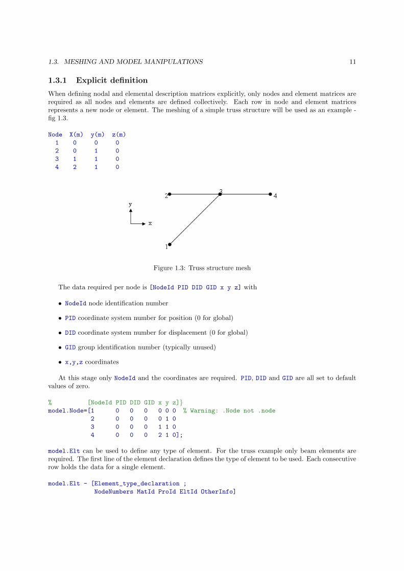
When defining nodal and elemental description matrices explicitly, only nodes and element matrices arerequired as all nodes and elements are defined collectively. Each row in node and element matricesrepresents a new node or element. The meshing of a simple truss structure will be used as an example -fig 1.3.

Node X(m) y(m) z(m)

1 0 0 0

2 0 1 0

3 1 1 0

4 2 1 0

Figure 1.3: Truss structure mesh

The data required per node is [NodeId PID DID GID x y z] with

• NodeId node identification number

• PID coordinate system number for position (0 for global)

• DID coordinate system number for displacement (0 for global)

• GID group identification number (typically unused)

• x,y,z coordinates

At this stage only NodeId and the coordinates are required. PID, DID and GID are all set to defaultvalues of zero.

% [NodeId PID DID GID x y z]}model.Node=[1 0 0 0 0 0 0 % Warning: .Node not .node

2 0 0 0 0 1 0

3 0 0 0 1 1 0

4 0 0 0 2 1 0];

model.Elt can be used to define any type of element. For the truss example only beam elements arerequired. The first line of the element declaration defines the type of element to be used. Each consecutiverow holds the data for a single element.

model.Elt - [Element_type_declaration ;

NodeNumbers MatId ProId EltId OtherInfo]


Element type declaration is a row of the matrix that defines which elements are described in fol-lowing rows. The format of this row is [Inf abs(’EltName’)] where Inf marks a header line, EltNameis the element type name (for example beam1, quad4, ...) and abs gives the ASCII value of the elementname. See section 1.4 for more details.

NodeNumbers depending on the element type the number of nodes required to define it will vary. For abeam two nodes are required, the start NodeId and the end NodeId (entries must be separated by a space).

• MatId material ID number in model.pl (see sdtweb pl)

• ProId element property (e.g. section area) ID number in model.il (see sdtweb il)

• EltId element ID number which uniquely identifies element (this is rarely needed in SDT and canbe fixed using (sdtweb feutil#feutil.EltId)

• OtherInfo additional options. Examples of additional options are beam node off-sets, orientationof bending planes etc.

In this case it can be assumed that all beam sections are identical. MatId and ProId can be set to 1(only one material and one element property need to be defined), the properties of which will be discussedlater. For beams, columns 5-7 specify the orientation and the EltId can be stored in column 8).

dir=[0 0 1];

model.Elt=[Inf abs(’beam1’) 0;

2 3 1 1 dir ;

3 4 1 1 dir ;

1 3 1 1 dir ];

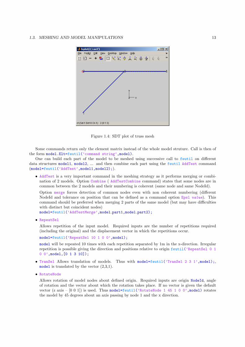
A graphical check can be performed using the feplot function - fig 1.4.

cf=feplot(model)

fecom(’triaxOn’); % Show triax

fecom(’textnode’,’GroupAll’,’FontSize’,12); %node numbers

The desired orientation can be selected from the figure toolbar.It is important to note at this stage that the true number of variables that can be entered for a beam

element far exceeds those shown here. When using the explicit definition of elements it is essential thatthe dimensions of all rows and all columns are equal – this includes the first line. In the case of a beamthe command [Inf abs(’beam1’)] accommodates six columns. All other rows must therefore have sixcolumns. This is why the options column, although not being used, must be defined (as zero in this case)if following rows are larger. Use of the additional options is easier when using a functional definition ofthe model.

1.3.2 Functional definition of meshes

It is impractical to explicitly define all but the simplest of models. A number of functions are available inthe SDT which allow manipulation of groups of elements in the assembly of a larger more complex model.This can be done in a piecemeal fashion, with sections of the complete model being added consecutively.

feutil function performs meshing operations (extrusion, repetitions, meshing some simple parts etc....).

The SDT uses command strings which define the specific action that the feutil (see sdtweb feutil)function performs. Typical call is following:

model=feutil(’command string’,model);


Figure 1.4: SDT plot of truss mesh

Some commands return only the element matrix instead of the whole model struture. Call is then ofthe form model.Elt=feutil(’command string’,model).

One can build each part of the model to be meshed using successive call to feutil on differentdata structures model1, model2, ... and then combine each part using the feutil AddTest command(model=feutil(’AddTest’,model1,model2);).

• AddTest is a very important command in the meshing strategy as it performs merging or combi-nation of 2 models. Option Combine ( AddTestCombine command) states that some nodes are incommon between the 2 models and their numbering is coherent (same node and same NodeId).

Option merge forces detection of common nodes even with non coherent numbering (differentNodeId and tolerance on position that can be defined as a command option Epsl value). Thiscommand should be preferred when merging 2 parts of the same model (but may have difficultieswith distinct but coincident nodes)model=feutil(’AddTestMerge’,model part1,model part2);

• RepeatSel

Allows repetition of the input model. Required inputs are the number of repetitions required(including the original) and the displacement vector in which the repetitions occur.

model=feutil(’RepeatSel 10 1 0 0’,model);

model will be repeated 10 times with each repetition separated by 1m in the x-direction. Irregularrepetition is possible giving the direction and positions relative to origin feutil(’RepeatSel 0 1

0 0’,model,[0 1 3 10]);

• TranSel Allows translation of models. Thus with model=feutil(’TranSel 2 3 1’,model);,model is translated by the vector (2,3,1).

• RotateNode

Allows rotation of model nodes about defined origin. Required inputs are origin NodeId, angleof rotation and the vector about which the rotation takes place. If no vector is given the defaultvector (z axis – [0 0 1]) is used. Thus model=feutil(’RotateNode 1 45 1 0 0’,model) rotatesthe model by 45 degrees about an axis passing by node 1 and the x direction.


feutil example 1:

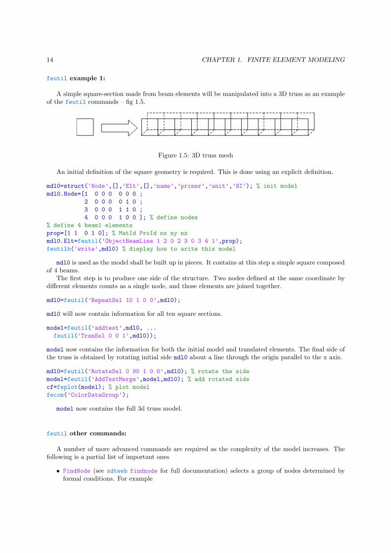
A simple square-section made from beam elements will be manipulated into a 3D truss as an exampleof the feutil commands – fig 1.5.

Figure 1.5: 3D truss mesh

An initial definition of the square geometry is required. This is done using an explicit definition.

mdl0=struct(’Node’,[],’Elt’,[],’name’,’primer’,’unit’,’SI’); % init model

mdl0.Node=[1 0 0 0 0 0 0 ;

2 0 0 0 0 1 0 ;

3 0 0 0 1 1 0 ;

4 0 0 0 1 0 0 ]; % define nodes

% define 4 beam1 elements

prop=[1 1 0 1 0]; % MatId ProId nx ny nz

mdl0.Elt=feutil(’ObjectBeamLine 1 2 0 2 3 0 3 4 1’,prop);

feutilb(’write’,mdl0) % display how to write this model

mdl0 is used as the model shall be built up in pieces. It contains at this step a simple square composedof 4 beams.

The first step is to produce one side of the structure. Two nodes defined at the same coordinate bydifferent elements counts as a single node, and those elements are joined together.

mdl0=feutil(’RepeatSel 10 1 0 0’,mdl0);

mdl0 will now contain information for all ten square sections.

model=feutil(’addtest’,mdl0, ...

feutil(’TranSel 0 0 1’,mdl0));

model now contains the information for both the initial model and translated elements. The final side ofthe truss is obtained by rotating initial side mdl0 about a line through the origin parallel to the x axis.

mdl0=feutil(’RotateSel 0 90 1 0 0’,mdl0); % rotate the side

model=feutil(’AddTestMerge’,model,mdl0); % add rotated side

cf=feplot(model); % plot model

fecom(’ColorDataGroup’);

model now contains the full 3d truss model.

feutil other commands:

A number of more advanced commands are required as the complexity of the model increases. Thefollowing is a partial list of important ones

• FindNode (see sdtweb findnode for full documentation) selects a group of nodes determined byformal conditions. For example


Figure 1.6: SDT plot of a 3D truss mesh

NodeId=feutil(’FindNode x==0 & y>=1’,model);

All nodes lying on the line x=0 and with y>=1 would be found. For display see fecom TextNode

and fecom ShowNodeMark;

• FindElt (see sdtweb findelt for full documentation) selects elements trough formal conditions.For display see fecom Sel.

• ObjectBeamLine Creates multiple or single beams between defined nodes. Other object commandsexist of plates, volumes, ...

model.Elt=feutil(’ObjectBeamLine 1:5’,prop) generates four beam elements from nodes 1-2,2-3 etc.

• Extrude

Allows extrusion of the selected elements. Required inputs are number of repetitions of the ex-trusion and the displacement vector in which the extrusions occur. Extrusion changes the elementtype: mass → beam, beam → quad, quad → hexa, ...

model=feutil(’Extrude 5 1 0 0’,model);

If the input model was a mass then the resultant would be 5 beam elements each 1 m long, orientatedin the x-direction.The extrusion command reduces the number of explicit element definitions that the user has tomake. For example, when meshing a plate the explicit definition of only two nodes is required.

feutil example 2:

The three commands listed above greatly reduce the volume of code required to generate largermeshes. The example of a right angled stiffener will be used. The mesh will consist of quad4

elements. Each element is 2x1 cm.

Two nodes are defined at coordinates (0,0,0) and (0,1,0). The ObjectBeamLine command can nowbe used to define a beam element represented by the red line on figure 1.7 (nodes 1 and 2).

md0=struct(’Node’,[],’Elt’,[],’name’,’primer’,’unit’,’SI’); % init model

mdl0.Node=[1 0 0 0 0 0 0 ;

2 0 0 0 0 1 0 ];

mdl0.Elt=feutil(’ObjectBeamLine 1 2’); % create beam between node 1 and 2


Figure 1.7: Right angled stiffener meshh

This single beam element can now be extruded into plate elements. Note that the output argumentis now a model since new nodes are added by the extrusion.The six plate elements are then repeatedin the y direction.

mdl0=feutil(’Extrude 6 2 0 0’,mdl0); % extrude the beam along x as 6 quads

mdl0=feutil(’RepeatSel 2 0 1 0’,mdl0); % repeat mdl0

model=mdl0; % first step of final model

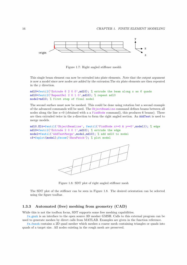
The second surface must now be meshed. This could be done using rotation but a second exampleof the advanced commands will be used. The ObjectBeamLine command defines beams between allnodes along the line x=0 (obtained with a a FindNode command), this produces 6 beams). Theseare then extruded twice in the z-direction to form the right angled section. An AddTest is used tomerge models.

mdl0.Elt=feutil(’ObjectBeamLine’, feutil(’FindNode x>=0 & y==0’,model)); % edge

mdl0=feutil(’Extrude 2 0 0 1’,mdl0); % extrude the edge

model=feutil(’AddTestMerge’,model,mdl0); % add mdl0 to model

cf=feplot(model);fecom(’ShowPatch’); % plot model

Figure 1.8: SDT plot of right angled stiffener mesh

The SDT plot of the stiffener can be seen in Figure 1.8. The desired orientation can be selectedusing the figure toolbar.

1.3.3 Automated (free) meshing from geometry (CAD)

While this is not the toolbox focus, SDT supports some free meshing capabilities.fe gmsh is an interface to the open source 3D mesher GMSH. Calls to this external program can be

used to generate meshes by direct calls from MATLAB. Examples are given in the function reference.fe fmesh contains a 2D quad mesher which meshes a coarse mesh containing triangles or quads into

quads of a target size. All nodes existing in the rough mesh are preserved.

1.4. ELEMENTS 17

% build rough mesh

model=feutil(’Objectquad 1 1’,[0 0 0;2 0 0; 2 3 0; 0 3 0],1,1);

model=feutil(’Objectquad 1 1’,model,[2 0 0;8 0 0; 8 1 0; 2 1 0],1,1);

feplot(model)

% start the mesher with a reference distance of .1

model=fe_fmesh(’qmesh .1’,model.Node,model.Elt);

model.name=’Qmesh test’; model.unit=’SI’;

feplot(model);

1.4 Elements

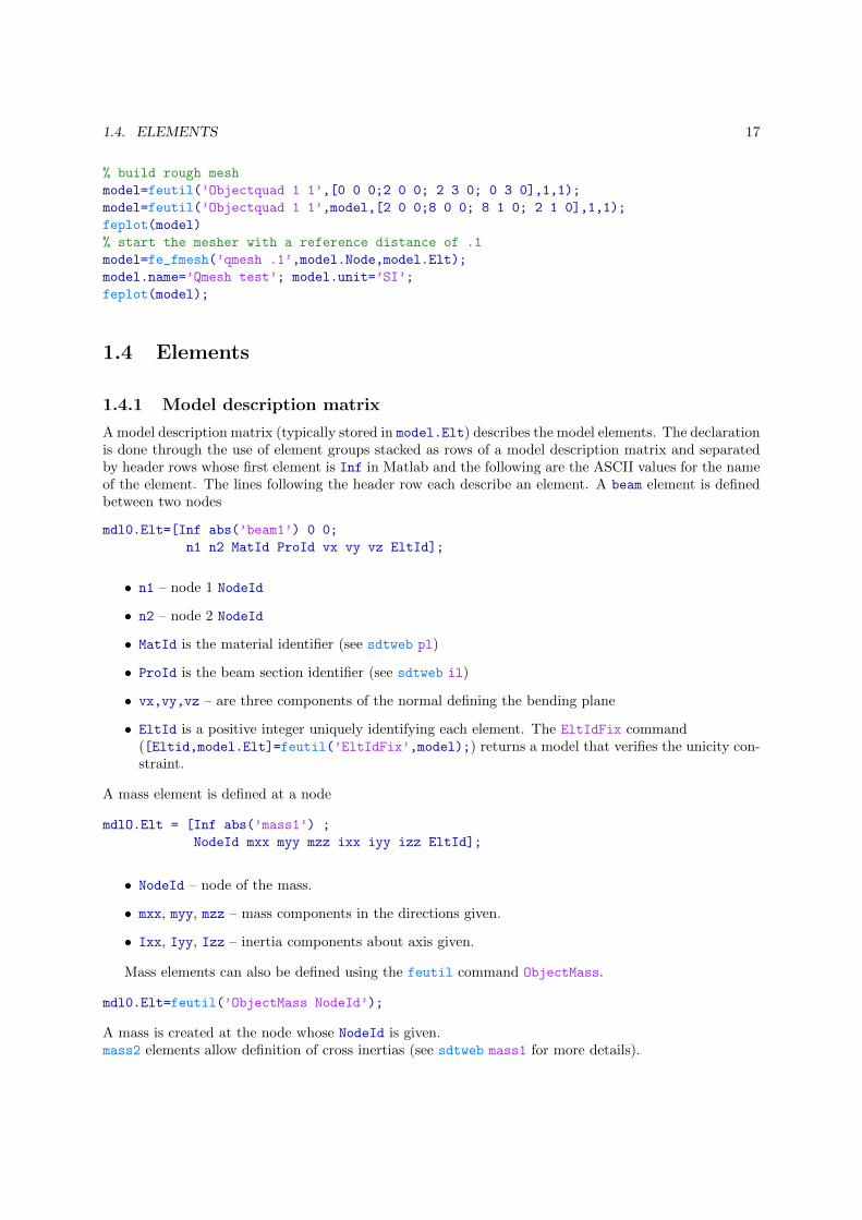
1.4.1 Model description matrix

A model description matrix (typically stored in model.Elt) describes the model elements. The declarationis done through the use of element groups stacked as rows of a model description matrix and separatedby header rows whose first element is Inf in Matlab and the following are the ASCII values for the nameof the element. The lines following the header row each describe an element. A beam element is definedbetween two nodes

mdl0.Elt=[Inf abs(’beam1’) 0 0;

n1 n2 MatId ProId vx vy vz EltId];

• n1 – node 1 NodeId

• n2 – node 2 NodeId

• MatId is the material identifier (see sdtweb pl)

• ProId is the beam section identifier (see sdtweb il)

• vx,vy,vz – are three components of the normal defining the bending plane

• EltId is a positive integer uniquely identifying each element. The EltIdFix command([Eltid,model.Elt]=feutil(’EltIdFix’,model);) returns a model that verifies the unicity con-straint.

A mass element is defined at a node

mdlO.Elt = [Inf abs(’mass1’) ;

NodeId mxx myy mzz ixx iyy izz EltId];

• NodeId – node of the mass.

• mxx, myy, mzz – mass components in the directions given.

• Ixx, Iyy, Izz – inertia components about axis given.

Mass elements can also be defined using the feutil command ObjectMass.

mdl0.Elt=feutil(’ObjectMass NodeId’);

A mass is created at the node whose NodeId is given.mass2 elements allow definition of cross inertias (see sdtweb mass1 for more details).


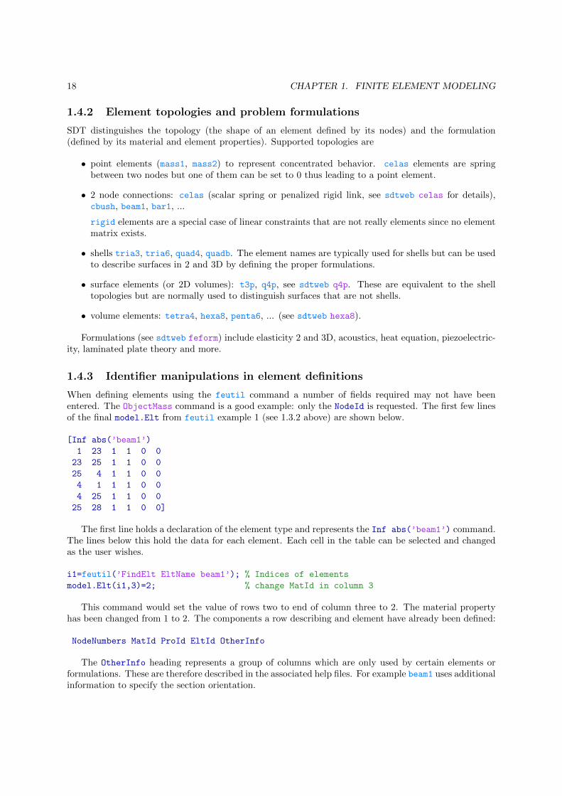
1.4.2 Element topologies and problem formulations

SDT distinguishes the topology (the shape of an element defined by its nodes) and the formulation(defined by its material and element properties). Supported topologies are

• point elements (mass1, mass2) to represent concentrated behavior. celas elements are springbetween two nodes but one of them can be set to 0 thus leading to a point element.

• 2 node connections: celas (scalar spring or penalized rigid link, see sdtweb celas for details),cbush, beam1, bar1, ...

rigid elements are a special case of linear constraints that are not really elements since no elementmatrix exists.

• shells tria3, tria6, quad4, quadb. The element names are typically used for shells but can be usedto describe surfaces in 2 and 3D by defining the proper formulations.

• surface elements (or 2D volumes): t3p, q4p, see sdtweb q4p. These are equivalent to the shelltopologies but are normally used to distinguish surfaces that are not shells.

• volume elements: tetra4, hexa8, penta6, ... (see sdtweb hexa8).

Formulations (see sdtweb feform) include elasticity 2 and 3D, acoustics, heat equation, piezoelectric-ity, laminated plate theory and more.

1.4.3 Identifier manipulations in element definitions

When defining elements using the feutil command a number of fields required may not have beenentered. The ObjectMass command is a good example: only the NodeId is requested. The first few linesof the final model.Elt from feutil example 1 (see 1.3.2 above) are shown below.

[Inf abs(’beam1’)

1 23 1 1 0 0

23 25 1 1 0 0

25 4 1 1 0 0

4 1 1 1 0 0

4 25 1 1 0 0

25 28 1 1 0 0]

The first line holds a declaration of the element type and represents the Inf abs(’beam1’) command.The lines below this hold the data for each element. Each cell in the table can be selected and changedas the user wishes.

i1=feutil(’FindElt EltName beam1’); % Indices of elements

model.Elt(i1,3)=2; % change MatId in column 3

This command would set the value of rows two to end of column three to 2. The material propertyhas been changed from 1 to 2. The components a row describing and element have already been defined:

NodeNumbers MatId ProId EltId OtherInfo

The OtherInfo heading represents a group of columns which are only used by certain elements orformulations. These are therefore described in the associated help files. For example beam1 uses additionalinformation to specify the section orientation.

1.5. MATERIAL AND ELEMENT PROPERTIES 19

1.5 Material and element properties

1.5.1 Material Properties

Materials are typically defined as rows of a pl matrix stored as the model.pl field (they can also be storedas mat stack entries in cases where a lot of data is needed : for temperature sensitivity for example).

Each material formulation should be associated with a m or p function. m elastic for elasticity andacoustics, m piezo for piezoelectric materials, p heat for the heat equation, ...

High level calls use these functions which contain a databases. Typical high level calls are

m_elastic info % prints the database to the screen

model.pl=m_elastic(’dbval 1 Steel’)

model.pl=m_elastic(model.pl,’dbval 2 Aluminum’)

These calls build model.pl where each row of the matrix represents a different material. The definitionbelow is for standard isotropic materials.

Default units are SI, but you can use m elastic(’dbval 1 -unit IN Steel’) for a conversion, seesdtweb fe mat#Convert

pl=[MatId E nu rho G eta alpha T0]

• MatId – material ID number as defined by user.

• type – type of material being used, typically fe mat(’m elastic’,’SI’,subtype). In the presentcase should be fe mat(’m elastic’,’SI’,1)

• E – Young’s modulus.

• nu – Poisson’s ratio.

• rho – density.

These five are the only required inputs – the following four are optional and are set to their defaultsif omitted.

• G – shear modulus (default set to G = E/2(1 + nu)).

• eta – hysteretic damping loss factor (default set to 0).

• alpha – thermal expansion coefficient.

• T0 – reference temperature.

For example the material definition matrix for aluminum in SI units would be

model.pl=[1 fe_mat(’m_elastic’,’SI’,1) 7.2e9 0.3 2700]


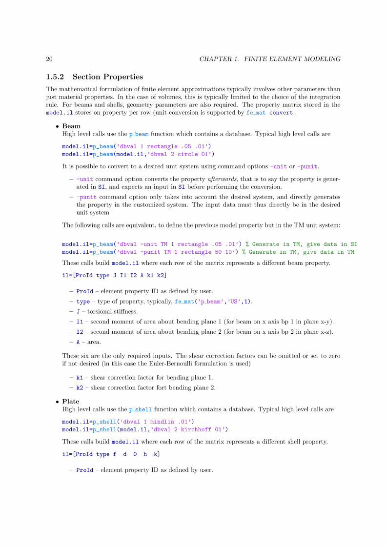
1.5.2 Section Properties

The mathematical formulation of finite element approximations typically involves other parameters thanjust material properties. In the case of volumes, this is typically limited to the choice of the integrationrule. For beams and shells, geometry parameters are also required. The property matrix stored in themodel.il stores on property per row (unit conversion is supported by fe mat convert.

• BeamHigh level calls use the p beam function which contains a database. Typical high level calls are

model.il=p_beam(’dbval 1 rectangle .05 .01’)

model.il=p_beam(model.il,’dbval 2 circle 01’)

It is possible to convert to a desired unit system using command options -unit or -punit.

– -unit command option converts the property afterwards, that is to say the property is gener-ated in SI, and expects an input in SI before performing the conversion.

– -punit command option only takes into account the desired system, and directly generatesthe property in the customized system. The input data must thus directly be in the desiredunit system

The following calls are equivalent, to define the previous model property but in the TM unit system:

model.il=p_beam(’dbval -unit TM 1 rectangle .05 .01’) % Generate in TM, give data in SI

model.il=p_beam(’dbval -punit TM 1 rectangle 50 10’) % Generate in TM, give data in TM

These calls build model.il where each row of the matrix represents a different beam property.

il=[ProId type J I1 I2 A k1 k2]

– ProId – element property ID as defined by user.

– type – type of property, typically, fe mat(’p beam’,’US’,1).

– J – torsional stiffness.

– I1 – second moment of area about bending plane 1 (for beam on x axis bp 1 in plane x-y).

– I2 – second moment of area about bending plane 2 (for beam on x axis bp 2 in plane x-z).

– A – area.

These six are the only required inputs. The shear correction factors can be omitted or set to zeroif not desired (in this case the Euler-Bernoulli formulation is used)

– k1 – shear correction factor for bending plane 1.

– k2 – shear correction factor fort bending plane 2.

• PlateHigh level calls use the p shell function which contains a database. Typical high level calls are

model.il=p_shell(’dbval 1 mindlin .01’)

model.il=p_shell(model.il,’dbval 2 kirchhoff 01’)

These calls build model.il where each row of the matrix represents a different shell property.

il=[ProId type f d 0 h k]

– ProId – element property ID as defined by user.

1.6. LOADS AND BOUNDARY CONDITIONS 21

– type – type of property, typically, fe mat(’p shell’,1,1).

– h – plate thickness.

– f – optional formulation selection.

– d – optional selection of stiffness coefficient for drilling DOF.

– k – shear correction factor for element formulations that support its use.

It is worth noting that a standard Matlab matrix must have the same number of columns in eachrow and vice versa. Care must be taken to ensure that this condition is not violated when storingproperties of elements of different types in the same matrix. Additional rows or columns can befilled by entering a zero. Other elements will be described further in later sections. For example:

il=[1 fe_mat(’p_beam’,’SI’,1) 1e-6 1e-7 1e-7 1e-4 0.8 ;

2 fe_mat(’p_shell’,’SI’,1) 1 1 0 5e-3 0 ];

The first row – element section property 1 (first column) – is a beam section definition. The secondrow is a plate definition. As the shear correction factor for plane 1 has been included for the beamproperty the final column of row two must be filled if all rows are to be of the same dimension.

• Spring and dashpot properties are supported with p spring.

• p solid supports integration rule selection for all elements that have all other properties definedin the material entry.

1.6 Loads and boundary conditions

All the loads and boundary conditions are handled with the fe case function and currently only oneglobal case is used at one time.

Before a model can be solved the boundary conditions must be considered.The fe case functions allows boundary conditions and loads to be declared. Each declaration is

stored as a different entry of the case stack, allowing multiple conditions to be applied. Any declarationapplies to the model data structure and uses the fe case format

model=fe_case(model,command1,command2, ...)

with commands following the format

’EntryType’,’Entry Name’,Data

To understand the calls, a little information of degree of freedom coding is needed.

1.6.1 Degrees of freedom

Each node has up to 99 degrees of freedom. By convention, the first 6 DOFs are three translationsand rotations (for other conventions see sdtweb mdof).

x-trans y-trans z-trans x-rot y-rot z-rot p T ....01 .02 .03 .04 .05 .06 .19 .20 ...

DOFs are coded with an integer part giving the node number and the first two dgits after the decimalgiving the DOF number NodeId.DofId. Thus 220.06 is the rotation of node 220 about the z-axis. Whenmanipulating matrices or results, DOFs are stored in a DOF definition vector (def.DOF, model.DOF, ...).

Before solving the model the active DOFs are resolved based on the element topologies and formula-tions by calling model.DOF=feutil(’GetDof’,model) (you really don’t have to do it by yourself).

fe c(DOF) returns a cell array giving the meaning of DOF in a vector. ind=fe c(DOF,adof,’ind’) isused to find the location of DOF �adof in vector DOF. fe c supports a number of other DOF manipulations.


1.6.2 Fixed boundary conditions

The entry type is FixDof (declared DOFs fixed). The name is arbitrarily defined by the user and isused as a reference to the boundary condition being applied. The data holds the list of DOFs that thecommand will apply to. There are a number of options on the type of data that can be entered.

• A global declaration of DOFs can be given as a column vector. For example [.03 .04 .05]’

would activate a 2-D simulation with only DOFs in x-trans, y-trans and z-rot being active becauseall z-trans, x-rot and y-rot DOF are fixed.

• A specific declaration of DOFs can be given as a column vector . For example [1.04 7.01 12]’

will fix x-rot at node 1, x-trans at node 7 and all DOFs at node 12).

• A FindNode command can be given as a string (see sdtweb FindNode for details). For example

model=fe_case(model,’FixDof’, ’LeftEdge’, ’x==0 -DOF 2 3’);

fixes DOFs 2 and 3 (translation y and z) along the line of nodes that verify x=0. In the structuresdefined in the examples above this represents the left edge, hence the name given.

1.6.3 Loads

DofLoad entries are used to apply loads on specified DOFs. When giving a list of DOFs, a unit load isapplied to each DOF (there are as many loads as DOFs in the list). To apply combined loads (a singleload on multiple DOF), you need to define a set of values on these loads through a structure

data=struct(’DOF’, Dof_declaration, ’def’, load_array);

The DOF declaration is a column vector of the DOFs to which the loads apply. The load arraycontains a number of column vectors, each of which represents a different loading condition. Thus for

DOF =

1.032.013.01

load =

1 00 10 −1

(1.1)

DOFs 1z, 2x and 3x are being loaded. The first column of the def array returns a unit load on DOF1z. The second column returns a positive unit load at DOF 2x and a negative at DOF 3x in the x, thisis typical of a relative load.

For distributed loads, see sdtweb fe load FVol and FSurf.

1.7 Solving

There are a number of solver functions. fe simul provides high level integrated solutions that combinemodel assembly and resolution for static, modal and time and frequency responses. More specific solversfe eig for eigenvalues, fe time for time domain or non-linear statics, fe2ss for state-space model buildingor fe reduc for model reduction provide more specialized calls with more options.

1.7. SOLVING 23

1.7.1 fe simul generic integrated solver

The fe simul function is the generic function to compute various types of response. Once you havedefined a FEM model, material and elements properties, loads and boundary conditions calling fe simul

assembles the model (if necessary) and computes the response using the dedicated algorithm. The genericcall is

[def,mo1] = fe_simul(’command’,model)

Where model is your FE model data structure and def is the deformation result (data structuredetailed in the post-processing section).

Accepted commands are ’Static’, ’Mode’, ’Time’, or ’Dfrf’.To control the assembly steps use the optimized assembly strategies (see sdtweb simul#s*feass) or

low level fe mknl calls.

1.7.2 fe eig real eigenvalue solution

The fe eig function returns the eigendata – including both mode shape and natural frequencies – in astructured matrix with fields .def for shapes, .DOF to code the DOFs of each row in .def and .data

giving the modal frequencies in Hz. The model matrix is the required input.

eigopt=[SolutionMethod nm Shift Print Thres];

def=fe_eig(model,eigopt);

Of the five possible options only the first two are required. The final three should be set to zero (thedefault values will be assigned).

• SolutionMethod – integer defines solution method. Default method is a full solution which canonly be used for simple models. For larger models use Lanczos solver 5.

• nm – number of modes required. The default value is a full analysis i.e. one mode for every degreeof freedom.

1.7.3 fe time full model transient and NL analysis

The fe time function allows analysis of the transient or non-linear response. It returns the deformationdata structure def and the model data structure (optional). Each column of the def.def array representsa time step or non-linear increment and the rows represent the DOF.

[def,model] = fe_time(’command’,model)

command – type of solver used. Newmark or dg (Discontinuous Galerkin) for example. You can alsouse a call of the form

model=stack_set(model,’info’,’TimeOpt’,data)

[def,model] = fe_time(model)

with time options in data having at least fields .Method and .Opt .TimeOpt.Method – string defining time integration algorithm (’Newmark’, ’dg’...).TimeOpt.Opt – line vector containing numeric options. For Newmark algorithms [beta gamma t0 dt

Ns] with beta=0.25, gamma=0.5 as defaults, t0 – Beginning of time simulation, dt – Time step, Ns –Number of steps to be computed.

For example:


model=stack_set(model,’curve’,’q0’,[]); % no initial deformation

TimeOpt=struct(’Method’,’newmark’, ...

’Opt’,[.25 .5 0 .1 20]);

model=stack_set(model,’info’,’TimeOpt’,TimeOpt);

def=fe_time(model);

Newmark solver used for model case 1. Zero initial conditions. Default values of beta and alpha used.Simulation begins at t=0, the time step is 0.1 s, there are 20 cycles computed.

1.7.4 nor2xf, modal frequency response

The nor2xf function allows FRFs to be evaluated using a modal basis. A required input is a set of modes(as calculated by fe eig). The location of both sensor and loading point by which it is excited are alsorequired. A case must therefore be defined, but it is done in a slightly different way.

load=struct(’DOF’,[14.03],’def’,[1]);

Case=fe_case(’DofLoad’,’loading’,load,’SensDof’,’sensor’,[14 15 16]’+.03);

As the deformations have already been calculated the model matrix is not needed. Loading and sensorplacement are given as before. Before the response can be calculated the frequency points at which itis required must be given. This is commonly done using the Matlab linspace function. The range ofvalues (start and end) and the total number of data points are inputted.

freq=linspace(start,end,no_points);

xf=nor2xf(def,damping,Case,freq,’command’);

• def – deformation matrix. This is obtained using the fe eig function.

• damping – damping ratio (0-1).

• Case – load case and sensor placement definition.

• freq – points at which frequency response calculated.

• command – optional command used to define units of frequency response.

For example:

freq=linspace(5,70,500);

nor2xf(def,.01,Case,IIw,’Hz iiplot -po "CurveName"’);

Response measured at 500 equally spaced frequency points between 5 to 70 Hz (the units are definedby the Hz in the command). A damping ratio of 0.01 is used. The iiplot -po "CurveName" appends adataset CurveName to the current iiplot figure (see section 1.8.2 or sdtweb diiplot).

1.8 Post-processing

1.8. POST-PROCESSING 25

1.8.1 feplot

The feplot function allows geometry display and deformation animation for both analysis and test. Inorder to manipulate the feplot you must open the figure and the associated GUI, display a model andpossibly deformations. A typical call is thus

cf=feplot(2); % open feplot in figure 2, store handle in cf variable

cf.model=model; % store model in the figure that cf points to

cf.def=def; % display deformation in this figure

cf=feplot(model,def) is a shortcut declaring model and deformations in a single call. Declaringa figure number is useful to force multiple feplot figures. The figure stores data using data structuresdetailed below.

• model=cf.mdl is a pointer to the model (see sdtweb model) stored in the figure

• def=cf.def deformation data structure (see sdtweb def). Fields are .DOF field (column vector), a.def field (matrix) whose number of rows is the same as .DOF vector and each column is a set ofdeformation (one modal deformation or one deformation at one time step, ...) and .data with asmany rows as .def columns defining time steps, frequencies, ...

In this example an animated plot of natural frequencies and mode shapes follows from fe eig

model=femesh(’Testubeam’); % simple ubeam example model

def=fe_eig(model,[5 10 1e3]);

cf=feplot(model,def)

The def structure holds mode shape data for the first 10 natural frequencies (including rigid bodymodes here). Having a figure handle cf, one can use cf.def=def to show def on the model displayed,and cf.def=[] to reset them.

In this other example a time response is considered

model=fe_time(’demo 2d’);

model=fe_time(’TimeOpt Newmark .25 .5 0 1e-4 50 10’,model);

def=fe_time(model); % compute the response

cf=feplot(model,def);

fecom(’AnimTime’)

The AnimTime command switches animation mode (time scans trough steps, while frequency uses acomplex scaling factor). Scaling of the amplitude is often necessary with the time response, this can be

done using the feplot GUI button , the l,L key (see sdtweb iimouse#key). Alternatively the fecom

commands can be used in the code to make changes programmatically (see sdtweb fecom).

1.8.2 iiplot

iiplot supports frequency/time data viewing. The data is stored into the figure and can be accessedthrough a pointer ci=iiplot;ci.Stack, see more details with sdtweb diiplot#CurveStack. The func-tion support data superposition, scanning through multiple channels, signal processing (illustrated in the

complete example below), ... Use the properties button to open the GUI tabs giving you graphicalaccess to a wide range of capabilities and see sdtweb iicom for a more complete list.


1.9 A complete example

The following example illustrates all functions and commands that have been introduced to this point.The structure being modeled is the right angled stiffener already described.

% Mesh -------------------------------------------------------------

mdl0=struct(’Node’,[],’Elt’,[],’name’,’primer’,’unit’,’SI’); % Init

% initial node declaration

mdl0.Node=[1 0 0 0 0 0 0;

2 0 0 0 0 .1 0];

mdl0.Elt=feutil(’ObjectBeamLine’,feutil(’FindNode x==0 & y<=1’,mdl0));

mdl0=feutil(’Extrude 6 .2 0 0’,mdl0);

% beam element created and extruded to make first row of plate elements

mdl0=feutil(’RepeatSel 2 0 .1 0’,mdl0);

% plates repeated to make one side of stiffener

model=mdl0;

% elements in temp mdl0 are put in model as group 1

mdl0.Elt=feutil(’ObjectBeamLine’,feutil(’FindNode x>=0 & y==0’,mdl0));

% beam elements created between nodes along line y=0

mdl0=feutil(’Extrude 2 0 0 .1’,mdl0);

% beam elements extruded to plate elements

model=feutil(’AddTestMerge’,model,mdl0);

% merge model and mdl0, mdl0 is in group 2 of new model

% Material and element properties -------------------------------------

model.pl=[1 fe_mat(’m_elastic’,’SI’,1) 7.2e9 .3 2700 2.68e10]; % material

model.il=[1 fe_mat(’p_shell’,’SI’,1) 0 0 0 5e-3]; % plate properties

% force MatId and ProId of both groups to be 1

model.Elt=feutil(’SetGroup 1 mat1 pro1’,model);

model.Elt=feutil(’SetGroup 2 mat1 pro1’,model);

% Loads and boundary conditions ----------------------------------------

load=struct(’DOF’,[14.03],’def’,[10]);

% load condition defined at node 14 orientated along z axis

model=fe_case(model, ...

’FixDof’,’left edge’,’x==0’,... % fix edge x==0

’DofLoad’,’endload’,load,... % apply load on 14z

’SensDof’,’tipsensor’,[14.03]); % place sensor on 14z

% Normal modes ---------------------------------------------------------

cf=feplot(model); model=cf.mdl;

cf.Stack{’info’,’EigOpt’}=[5 10 1e3];

% deformation calculated for model

% options: 5 - Lanczos solver

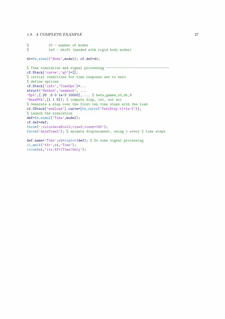
1.9. A COMPLETE EXAMPLE 27

% 10 - number of modes

% 1e3 - shift (needed with rigid body modes)

d1=fe_simul(’Mode’,model); cf.def=d1;

% Time simulation and signal processing --------------------------------

cf.Stack{’curve’,’q0’}=[];% initial conditions for time response set to zero

% define options

cf.Stack{’info’,’TimeOpt’}=...struct(’Method’,’newmark’, ...

’Opt’,[.25 .5 0 1e-3 10000], ... % beta,gamma,t0,dt,N

’NeedUVA’,[1 1 0]); % compute disp, vel, not acc

% Generate a step over the first ten time steps with the load

cf.CStack{’endload’}.curve={fe_curve(’TestStep t1=1e-2’)};% Launch the simulation

def=fe_simul(’Time’,model);

cf.def=def;

fecom(’;colordataEvalZ;view3;viewh+180’);

fecom(’AnimTime2’); % animate displacement, using 1 every 2 time steps

def.name=’Time’;ci=iiplot(def); % Do some signal processing

ii_mmif(’fft’,ci,’Time’);

iicom(ci,’iix:fft(Time)Only’);

2

Experimental modal analysis

Contents

2.1 Testing . . . . . . . . . . . . . . . . . . . . . . . . . . . . . . . . . . . . . . . . . 30

2.1.1 Measuring transfer functions . . . . . . . . . . . . . . . . . . . . . . . . . . . . 30

2.1.2 Multiple locations to get shapes . . . . . . . . . . . . . . . . . . . . . . . . . . . 31

2.2 Identification (mode extraction) . . . . . . . . . . . . . . . . . . . . . . . . . 31

2.2.1 Importing measurements into iiplot, idcom . . . . . . . . . . . . . . . . . . . . 31

2.2.2 Identified modal model . . . . . . . . . . . . . . . . . . . . . . . . . . . . . . . 33

2.2.3 Single mode peak picking method . . . . . . . . . . . . . . . . . . . . . . . . . 33

2.2.4 Multi-mode estimation and refinement method . . . . . . . . . . . . . . . . . . 34

2.3 Test geometry and visualization . . . . . . . . . . . . . . . . . . . . . . . . . . 34

2.3.1 Wire frame model . . . . . . . . . . . . . . . . . . . . . . . . . . . . . . . . . . 34

2.3.2 Sensor placement . . . . . . . . . . . . . . . . . . . . . . . . . . . . . . . . . . . 36

2.3.3 Visualizing test shapes (ODS, modes, ...) . . . . . . . . . . . . . . . . . . . . . 38

2.4 A complete modal test example . . . . . . . . . . . . . . . . . . . . . . . . . . 38

30 CHAPTER 2. EXPERIMENTAL MODAL ANALYSIS

Experimental modal analysis has the objective of characterizing modal properties (poles and mode-shapes) trough experiment, this tutorial will focus on the case where inputs are measured, but outputonly methods are also useful in many cases.

2.1 Testing

This is a very crude summary of the many issues associated with testing that are analyzed in moredetail in classical books [1, 2] or the course notes [3] available at www.sdtools.com/pdf/PolyId.pdf.

2.1.1 Measuring transfer functions

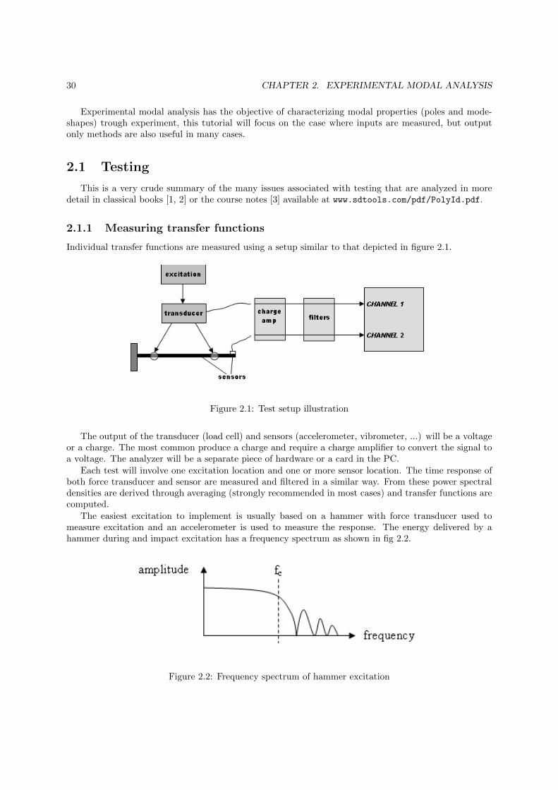
Individual transfer functions are measured using a setup similar to that depicted in figure 2.1.

Figure 2.1: Test setup illustration

The output of the transducer (load cell) and sensors (accelerometer, vibrometer, ...) will be a voltageor a charge. The most common produce a charge and require a charge amplifier to convert the signal toa voltage. The analyzer will be a separate piece of hardware or a card in the PC.

Each test will involve one excitation location and one or more sensor location. The time response ofboth force transducer and sensor are measured and filtered in a similar way. From these power spectraldensities are derived through averaging (strongly recommended in most cases) and transfer functions arecomputed.

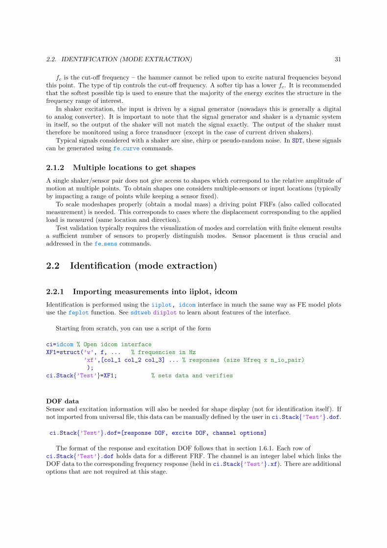
The easiest excitation to implement is usually based on a hammer with force transducer used tomeasure excitation and an accelerometer is used to measure the response. The energy delivered by ahammer during and impact excitation has a frequency spectrum as shown in fig 2.2.

Figure 2.2: Frequency spectrum of hammer excitation

www.sdtools.com/pdf/PolyId.pdf

2.2. IDENTIFICATION (MODE EXTRACTION) 31

fc is the cut-off frequency – the hammer cannot be relied upon to excite natural frequencies beyondthis point. The type of tip controls the cut-off frequency. A softer tip has a lower fc. It is recommendedthat the softest possible tip is used to ensure that the majority of the energy excites the structure in thefrequency range of interest.

In shaker excitation, the input is driven by a signal generator (nowadays this is generally a digitalto analog converter). It is important to note that the signal generator and shaker is a dynamic systemin itself, so the output of the shaker will not match the signal exactly. The output of the shaker musttherefore be monitored using a force transducer (except in the case of current driven shakers).

Typical signals considered with a shaker are sine, chirp or pseudo-random noise. In SDT, these signalscan be generated using fe curve commands.

2.1.2 Multiple locations to get shapes

A single shaker/sensor pair does not give access to shapes which correspond to the relative amplitude ofmotion at multiple points. To obtain shapes one considers multiple-sensors or input locations (typicallyby impacting a range of points while keeping a sensor fixed).

To scale modeshapes properly (obtain a modal mass) a driving point FRFs (also called collocatedmeasurement) is needed. This corresponds to cases where the displacement corresponding to the appliedload is measured (same location and direction).

Test validation typically requires the visualization of modes and correlation with finite element resultsa sufficient number of sensors to properly distinguish modes. Sensor placement is thus crucial andaddressed in the fe sens commands.

2.2 Identification (mode extraction)

2.2.1 Importing measurements into iiplot, idcom

Identification is performed using the iiplot, idcom interface in much the same way as FE model plotsuse the feplot function. See sdtweb diiplot to learn about features of the interface.

Starting from scratch, you can use a script of the form

ci=idcom % Open idcom interface

XF1=struct(’w’, f, ... % frequencies in Hz

’xf’,[col_1 col_2 col_3] ... % responses (size Nfreq x n_io_pair)

);

ci.Stack{’Test’}=XF1; % sets data and verifies

DOF dataSensor and excitation information will also be needed for shape display (not for identification itself). Ifnot imported from universal file, this data can be manually defined by the user in ci.Stack{’Test’}.dof.

ci.Stack{’Test’}.dof=[response DOF, excite DOF, channel options]

The format of the response and excitation DOF follows that in section 1.6.1. Each row ofci.Stack{’Test’}.dof holds data for a different FRF. The channel is an integer label which links theDOF data to the corresponding frequency response (held in ci.Stack{’Test’}.xf). There are additionaloptions that are not required at this stage.


Standard datasets

idcom uses standard datasets (for idcom the names are mandatory, but you can have other sets inthe same figure)

• Test measured transfer functions (main fields are .w frequencies, .xf responses, .dof sensor actu-ator definitions), see sdtweb(’curve#Response data’) for more details).

• IdFrf last identification result obtained using idcom commands

• IdMain principal set of identified modes, main fields are .po poles (first column with frequencies,second with damping ratio) and .res residues (one row per pole), see sdtweb(’curve#Shapes at

DOFs’) for more details).

• IdAlt alternate set of identified modes

These datasets are stored in the figure and more easily accessed by name

ci=idcom % obtain pointer to the figure

ci.Stack{’Test’} reference a dataset by its name

ci.Stack{’Test’}.dof(:,1) % get input DOFs

Identification options

Options relevant for the identification can be set in the idcom IDopt tab. They should be modifiedgraphically or using the ci.IDopt pointer. Typical values are shown below

>> ci=idcom; ci.IDopt

(ID options in figure(2)) =

ResidualTerms : [ 0 | 1 (1) | 2 (s^-2) | {3 (1 s^-2)} | 10 (1 s)]

DataType : [ disp./force | vel./force | {acc./force} ]

AbscissaUnits : [ {Hz} | rd/s | s ]

PoleUnits : [ {Hz} | rd/s ]

SelectedRange : [ 1-3124 (4.0039-64.9998) ]

FittingModel : [ Posit. cpx | {Complex modes} | Normal Modes]

NSNA : [ 1 sensor(s) 24 actuator(s) ]

Reciprocity : [ {Not used} | 1 FRF | MIMO ]

Collocated : [ none declared ]

Typical script modifications for data imported manually would be (see sdtweb idopt for more details)

ci.IDopt.Residual=3; % Force low and high frequency residual

ci.IDopt.DataType=’Acc’; % if acceleration was not set

ci.IDopt.Fit=’Complex’; % Use normal modes

ci.IDopt.NSNA=[24 1]; % declare number of sensors/actuators

Learn moreFurther details on import are discussed in sdtweb diiplot#xfread for both cases with raw vectors offrequencies and responses and cases where universal files are available (when this is the case, more infois already available and should be imported).

Results can be saved with idcom(’CurveSave’) or File:Curve save ... menu. They can bereloaded with ci=iicom(’CurveLoad’,’FileName.mat’), or File:Load curves from ... menu.

2.2. IDENTIFICATION (MODE EXTRACTION) 33

2.2.2 Identified modal model

Identification is the process by which a mathematical representation of FRF in the form of a series ofmodal contributions is obtained. The nominal spectral decomposition is associated to complex modesand leads to a representation of the transfer function of the form

[α(s)] =

2N∑j=1

([Rj ]

s− λj

)(2.1)

Each row of ci.Stack{’IdMain’}.po represents a pole λj . Except when forced otherwise, the firstcolumn contains the frequency (magnitude of pole) and the second column the damping ratio.

Each row of ci.Stack{’IdMain’}.res represents mode shape Rj . Each column represents a differentresponse channel i.e. a different actuator/sensor pair.

2.2.3 Single mode peak picking method

The modal model is constructed using FRFs. There are a number of methods used to extract this data,the method preferred in SDT is a gradual building of the model using sequential peak pickings, followedby refinement.

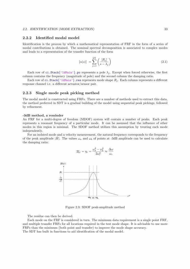
-3dB method, a reminderAn FRF for a multi-degree of freedom (MDOF) system will contain a number of peaks. Each peakrepresents a resonant frequency of a particular mode. It can be assumed that the influence of othermodes in this region is minimal. The SDOF method utilizes this assumption by treating each modeindependently.

For an isolated mode and a velocity measurement, the natural frequency corresponds to the frequencyof the peak amplitude |H|. The values ωa and ωb of points at -3dB amplitude can be used to calculatethe damping ratio:

2ξr = ηr =ω2a − ω2

b

2ω2r

≈ ∆ω

ωr

Figure 2.3: SDOF peak-amplitude method

The residue can then be derived.Each mode on the FRF is considered in turn. The minimum data requirement is a single point FRF,

and multiple transfer FRFs for all locations required in the test mode shape. It is advisable to use moreFRFs than the minimum (both point and transfer) to improve the mode shape accuracy.The SDT has built in functions to aid identification of the modal model.


idcom e

The idcom(’eband frequency’)’ command is a single pole estimator that is similar to the -3dBmethod but uses all transfers in Test simultaneously and allows for the presence of nearby modes. Youare expected to provide a frequency bandwidth trough band (number of points if ¿1, or fraction of centerfrequency if ¡1) and a center frequency for the search through frequency.

With no argument, idcom(’e’) uses the current bandwidth set in the idcom figure (default to 1%)and waits for a graphical input of the frequency in the iiplot figure.

Once a pole has been estimated it will appear on the iiplot as a IdFrf green curve over the testdata. If the estimate is accurate (this should determined by visual inspection) it should be added tothe main set of modeshapes ci.Stack{’IdMain’} with the idcom(’ea’) command or right arrow in theGUI.

A typical example would be

ci=idcom(’curveload gartid’);

idcom(’e .01 6.5’); % Estimate a first mode

idcom(’ea’) % Move it to the main set of modes

idcom(’e .01 34’); % Estimate a second mode

idcom(’ea’) % Move it to the main set of modes

idcom(’TableIdMain’) % Display poles in IdMain

2.2.4 Multi-mode estimation and refinement method

Once a sufficient number of modes are identified with peak picking, the next step is to obtain a broadbandmodel with multiple modes.

idcom(’est’) or the associated button will estimate the modes using the whole data currently selected(shown in iiplot). When the estimate is not accurate enough you should learn how to tune the polesusing the eopt and eup commands/buttons (see sdtweb idrc for details).

When dealing with data that is not very clean, you may find useful to estimate modeshapes using onlya fraction of the measured data around each resonance. This obtained with idcom(’estLocalPole’).

With both commands shapes and poles are stored in ci.Stack{’IdMain’} while synthesized responsesare in ci.Stack{’IdFrf’}.

2.3 Test geometry and visualization

2.3.1 Wire frame model

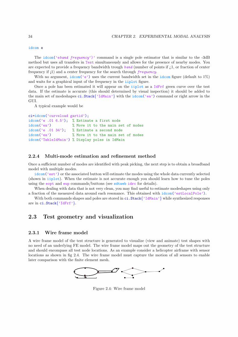
A wire frame model of the test structure is generated to visualize (view and animate) test shapes withno need of an underlying FE model. The wire frame model maps out the geometry of the test structureand should encompass all test node locations. As an example consider a helicopter airframe with sensorlocations as shown in fig 2.4. The wire frame model must capture the motion of all sensors to enablelater comparison with the finite element mesh.

Figure 2.4: Wire frame model

2.3. TEST GEOMETRY AND VISUALIZATION 35

A wire-frame geometry is composed of nodes and elements. It is important to remember that theelements used for the representation have no mechanical meaning. Steps for the definition of a wire-framemodel are (see sdtweb pre for more details).

• Declaration of nodes these should correspond to all the locations where a sensor is placed alongwith a number of additional nodes which aid visualization. Nodes can be declared in a script (seethe gartte demo for example) or added graphically in a feplot figure.

Input argument of fecom AddNode is a standard model node matrix (with 7 columns, [NodeId 0 0

0 x y z]), for example fecom(’AddNode’,[1001 0 0 0 1 0 0; 1002 0 0 0 2 2 2]);. One canalso only give a 3 column matrix with x y z positions but NodeIds are then assigned automatically.With no input, a dialog box opens that allows cut and paste (from Excel for example).

• Declaration of connectivity. Classically lines are used, with a call of the form fecom(’AddLine’,L)

with the L array holding the NodeId numbers for those nodes being connected, the line will becontinuous between all nodes given unless separated by a 0. For example

L=[1020 1023 1034 0 1012 1034 1039];

fecom(’AddLine’,L);

represents two lines between nodes: 1020-1023-1034 and 1012-1034-1039.

In the example below additional nodes (1003, 1007, 1009 ... ) are introduced to obtain a bet-ter modeshape visualization. But response at these nodes is not measured, extrapolation (calledexpansion) for proper animation will be discussed later.

• Declaration of sensors. In the simple case of sensors in global directions, just provide the NodeId.DofIdformat. If you have more general configurations, look the translation sensor documentation (sdtwebsensor#trans)

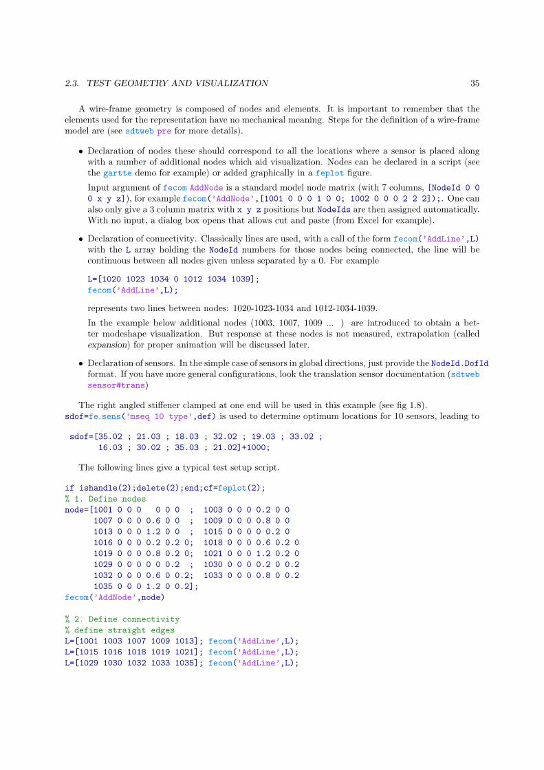
The right angled stiffener clamped at one end will be used in this example (see fig 1.8).sdof=fe sens(’mseq 10 type’,def) is used to determine optimum locations for 10 sensors, leading to

sdof=[35.02 ; 21.03 ; 18.03 ; 32.02 ; 19.03 ; 33.02 ;

16.03 ; 30.02 ; 35.03 ; 21.02]+1000;

The following lines give a typical test setup script.

if ishandle(2);delete(2);end;cf=feplot(2);

% 1. Define nodes

node=[1001 0 0 0 0 0 0 ; 1003 0 0 0 0.2 0 0

1007 0 0 0 0.6 0 0 ; 1009 0 0 0 0.8 0 0

1013 0 0 0 1.2 0 0 ; 1015 0 0 0 0 0.2 0

1016 0 0 0 0.2 0.2 0; 1018 0 0 0 0.6 0.2 0

1019 0 0 0 0.8 0.2 0; 1021 0 0 0 1.2 0.2 0

1029 0 0 0 0 0 0.2 ; 1030 0 0 0 0.2 0 0.2

1032 0 0 0 0.6 0 0.2; 1033 0 0 0 0.8 0 0.2

1035 0 0 0 1.2 0 0.2];

fecom(’AddNode’,node)

% 2. Define connectivity

% define straight edges

L=[1001 1003 1007 1009 1013]; fecom(’AddLine’,L);

L=[1015 1016 1018 1019 1021]; fecom(’AddLine’,L);

L=[1029 1030 1032 1033 1035]; fecom(’AddLine’,L);


% Define 5 L shaped edges as single 4th group

L=[1015 1001 1029 0 1016 1003 1030 0 1018 1007 1032 0 ...

1019 1009 1033 0 1021 1013 1035 0]; fecom(’AddLine’,L);

% 3. Define and show sensors

sdof=[35.02 ; 21.03 ; 18.03 ; 32.02 ; 19.03 ; 33.02 ;

16.03 ; 30.02 ; 35.03 ; 21.02]+1000;

cf.mdl=fe_case(cf.mdl,’SensDof’,’Test’,sdof);

fecom(’CurtabCases’,’Test’);fecom(’ProviewOn’);

fecom(’TriaxOn’);fecom(’TextNode’,’GroupAll’,’FontSize’,12)

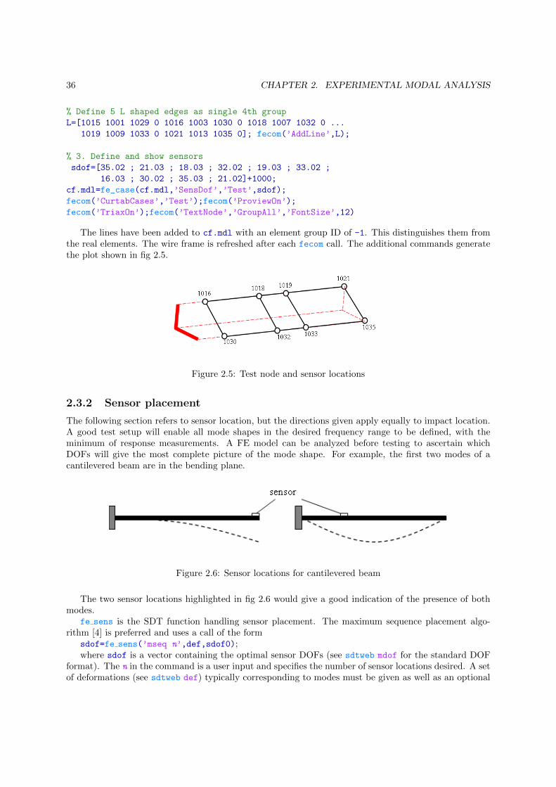
The lines have been added to cf.mdl with an element group ID of -1. This distinguishes them fromthe real elements. The wire frame is refreshed after each fecom call. The additional commands generatethe plot shown in fig 2.5.

Figure 2.5: Test node and sensor locations

2.3.2 Sensor placement

The following section refers to sensor location, but the directions given apply equally to impact location.A good test setup will enable all mode shapes in the desired frequency range to be defined, with theminimum of response measurements. A FE model can be analyzed before testing to ascertain whichDOFs will give the most complete picture of the mode shape. For example, the first two modes of acantilevered beam are in the bending plane.

Figure 2.6: Sensor locations for cantilevered beam

The two sensor locations highlighted in fig 2.6 would give a good indication of the presence of bothmodes.

fe sens is the SDT function handling sensor placement. The maximum sequence placement algo-rithm [4] is preferred and uses a call of the form

sdof=fe sens(’mseq n’,def,sdof0);where sdof is a vector containing the optimal sensor DOFs (see sdtweb mdof for the standard DOF

format). The n in the command is a user input and specifies the number of sensor locations desired. A setof deformations (see sdtweb def) typically corresponding to modes must be given as well as an optional

2.3. TEST GEOMETRY AND VISUALIZATION 37

initial set of sensors sdof0 that must be retained. Rotational DOFs are ignored du to the difficulty inmeasuring them.

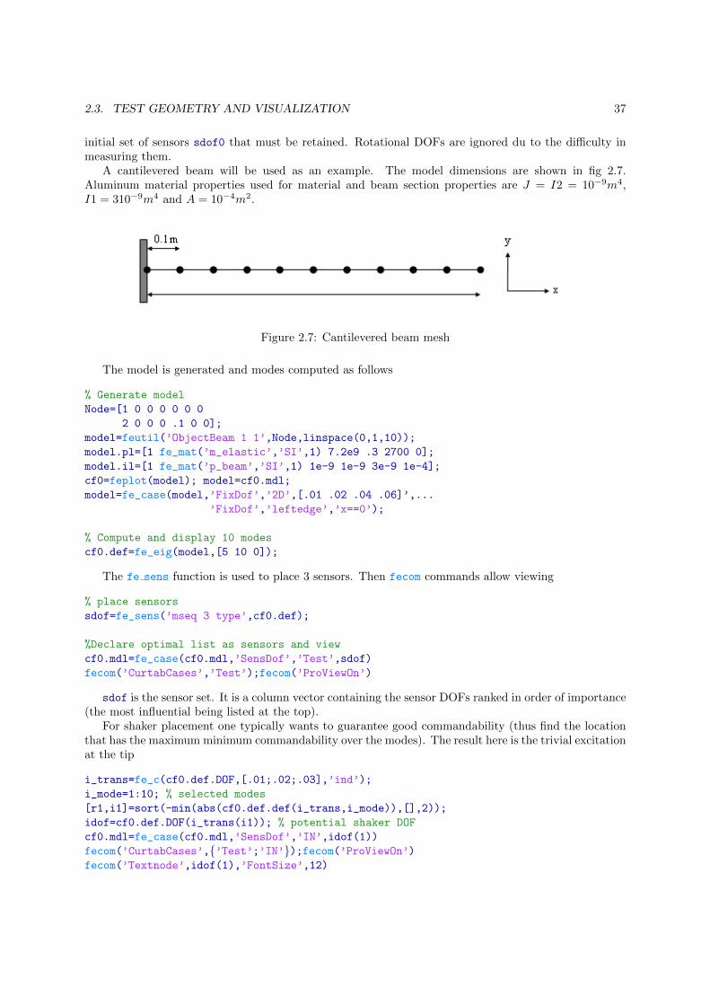
A cantilevered beam will be used as an example. The model dimensions are shown in fig 2.7.Aluminum material properties used for material and beam section properties are J = I2 = 10−9m4,I1 = 310−9m4 and A = 10−4m2.

Figure 2.7: Cantilevered beam mesh

The model is generated and modes computed as follows

% Generate model

Node=[1 0 0 0 0 0 0

2 0 0 0 .1 0 0];

model=feutil(’ObjectBeam 1 1’,Node,linspace(0,1,10));

model.pl=[1 fe_mat(’m_elastic’,’SI’,1) 7.2e9 .3 2700 0];

model.il=[1 fe_mat(’p_beam’,’SI’,1) 1e-9 1e-9 3e-9 1e-4];

cf0=feplot(model); model=cf0.mdl;

model=fe_case(model,’FixDof’,’2D’,[.01 .02 .04 .06]’,...

’FixDof’,’leftedge’,’x==0’);

% Compute and display 10 modes

cf0.def=fe_eig(model,[5 10 0]);

The fe sens function is used to place 3 sensors. Then fecom commands allow viewing

% place sensors

sdof=fe_sens(’mseq 3 type’,cf0.def);

%Declare optimal list as sensors and view

cf0.mdl=fe_case(cf0.mdl,’SensDof’,’Test’,sdof)

fecom(’CurtabCases’,’Test’);fecom(’ProViewOn’)

sdof is the sensor set. It is a column vector containing the sensor DOFs ranked in order of importance(the most influential being listed at the top).

For shaker placement one typically wants to guarantee good commandability (thus find the locationthat has the maximum minimum commandability over the modes). The result here is the trivial excitationat the tip

i_trans=fe_c(cf0.def.DOF,[.01;.02;.03],’ind’);

i_mode=1:10; % selected modes

[r1,i1]=sort(-min(abs(cf0.def.def(i_trans,i_mode)),[],2));

idof=cf0.def.DOF(i_trans(i1)); % potential shaker DOF

cf0.mdl=fe_case(cf0.mdl,’SensDof’,’IN’,idof(1))

fecom(’CurtabCases’,{’Test’;’IN’});fecom(’ProViewOn’)fecom(’Textnode’,idof(1),’FontSize’,12)


It should be noted that more than one shaker may be needed to excite all modes (for example formodes orthogonal to the shaker axis).

Figure 2.8: SDT plot of cantilever beam sensor placement

fecom commands can also be initialized using the feplot properties GUI (open with a click on the

button ).

2.3.3 Visualizing test shapes (ODS, modes, ...)

Having extracted the modal model a means to visualize the mode shapes is required. The deformationsare linked in with the wire frame model to produce an animated plot. The method used is a standardSDT feplot . It is assumed here that a wire frame has already been defined in the variable model.

cf=feplot(model);

fecom(cf,’ShowLine’);

To plot the mode shapes simply use cf.def=ci.Stack{’IdMain’}. You can also display FRFs withcf.def=ci.Stack{’Test’} (but in that case use the Cursor ...:ODS start context menu in iiplot).

It may be useful to understand the relation between test and FEM storage. Typicall def (as cf.def)has following field:

• .DOF – list of degrees of freedom to which the deformation applies. For test first column ofci.Stack{’IdMain’}.dof(:,1) gives the same information and id rm is used to deal with MIMOcases where sensors are repeated for multiple inputs).

• .data – natural frequencies corresponds to ci.Stack{’IdMain’}.po for poles or ci.Stack{’Test’}.wfor frequencies.

• .def – columns give mode shapes while ci.Stack{’IdMain’}.res rows give residues and ci.Stack{’Test’}.xfrows responses at sensors.

2.4 A complete modal test example

The example structure being used here is a tubular structure shown below.

2.4. A COMPLETE MODAL TEST EXAMPLE 39

Figure 2.9: Structure used in the modal test

The test data used was generated using SDT – a full testing example will be given separately.

% The data can be downloaded with

demosdt(’download http://www.sdtools.com/contrib/kart_example.mat’)

% www.sdtools.com/contrib/kart_example.mat

%----------

% WIRE FRAME DEFINITION (present in WIREFRAME) built with

%----------------------

WIREFRAME.Node=[ ...

1 0 0 0 0.613 0 0 ; 2 0 0 0 1.133 -0.198 0

3 0 0 0 1.548 -0.208 0 ; 4 0 0 0 1.538 -0.487 0

5 0 0 0 1.133 -0.51 0 ; 6 0 0 0 0.613 -0.742 0

7 0 0 0 0.32 0 0 ; 8 0 0 0 0.772 -0.287 0

9 0 0 0 0.772 -0.521 0 ; 10 0 0 0 0.33 -0.7483 0

11 0 0 0 0.41 -0.218 0 ; 12 0 0 0 0.38 -0.545 0

13 0 0 0 0.1 -0.22066 0; 14 0 0 0 0.1 -0.55167 0

15 0 0 0 0 -0.2177 0 ; 16 0 0 0 0 -0.544285 0

];

WIREFRAME.Elt=[];feplot(WIREFRAME)

fecom(’TextNode’);

% You can use the contextmenu (right click) cursor ... -> 3dline pick

feplot(’addline’,[4 3 2 1 7 15 16 10 6 5 4]) % add a first line

feplot(’addline’,[8 11 13 0 9 12 14 13 0 9 8 0 12 11]) % other line

% POLE ESTIMATION

%-----------------

% download and load test data :

demosdt(’download http://www.sdtools.com/contrib/kart_example.mat’)

ci=idcom; % open interface and get pointers ci

ci.Stack{’Test’}.w=TESTDATA.w; % Frequencies


ci.Stack{’Test’}.xf=TESTDATA.xf; % Responses

ci.Stack{’Test’}.dof=TESTDATA.dof; % Dofs

iicom(’SubMagPha’); % frequency response data plotted

% poles must now be identified one by one

idcom(’e .01 44.6’);

iicom(’CurTabIdent’)

% pole estimated at freq of 44.6Hz with possible range of .01 percent

% around that frequency.

% estimate checked on freq plot, if correct it is added

idcom(’ea’);

idcom(’e .01 48.8’); idcom(’ea’);

idcom(’e .01 95.3’); idcom(’ea’);

idcom(’e .01 125.3’);idcom(’ea’);

idcom(’e .01 141’); idcom(’ea’);

% five poles estimated in total and are stored in ci.Stack{’IdMain’}.po.% modeshapes are based on narrowband estimate.

idcom(’est’); % build a broad-band identification

% VISUALISATION

%---------------

cf=feplot; cf.model=WIREFRAME; % plot WIREFRAME test model

cf.def=ci.Stack{’IdMain’}; fecom(’view3’) % display identified shapes

3

Correlation

Contents

3.1 Topology correlation . . . . . . . . . . . . . . . . . . . . . . . . . . . . . . . . 42

3.2 Correlation criteria . . . . . . . . . . . . . . . . . . . . . . . . . . . . . . . . . 42

3.2.1 Modal Assurance Criteria (MAC) . . . . . . . . . . . . . . . . . . . . . . . . . . 42

3.2.2 Auto MAC . . . . . . . . . . . . . . . . . . . . . . . . . . . . . . . . . . . . . . 43

3.2.3 Standard MAC . . . . . . . . . . . . . . . . . . . . . . . . . . . . . . . . . . . . 43

3.2.4 COMAC . . . . . . . . . . . . . . . . . . . . . . . . . . . . . . . . . . . . . . . . 43

3.2.5 eCOMAC . . . . . . . . . . . . . . . . . . . . . . . . . . . . . . . . . . . . . . . 44

3.3 Modeshape expansion . . . . . . . . . . . . . . . . . . . . . . . . . . . . . . . . 44

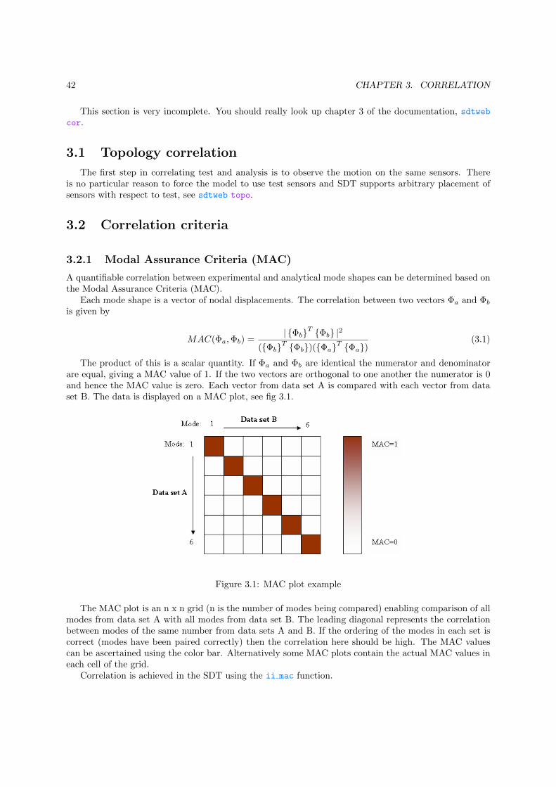
42 CHAPTER 3. CORRELATION

This section is very incomplete. You should really look up chapter 3 of the documentation, sdtwebcor.

3.1 Topology correlation

The first step in correlating test and analysis is to observe the motion on the same sensors. Thereis no particular reason to force the model to use test sensors and SDT supports arbitrary placement ofsensors with respect to test, see sdtweb topo.

3.2 Correlation criteria

3.2.1 Modal Assurance Criteria (MAC)

A quantifiable correlation between experimental and analytical mode shapes can be determined based onthe Modal Assurance Criteria (MAC).

Each mode shape is a vector of nodal displacements. The correlation between two vectors Φa and Φb

is given by

MAC(Φa,Φb) =| {Φb}T {Φb} |2

({Φb}T {Φb})({Φa}T {Φa})(3.1)

The product of this is a scalar quantity. If Φa and Φb are identical the numerator and denominatorare equal, giving a MAC value of 1. If the two vectors are orthogonal to one another the numerator is 0and hence the MAC value is zero. Each vector from data set A is compared with each vector from dataset B. The data is displayed on a MAC plot, see fig 3.1.

Figure 3.1: MAC plot example

The MAC plot is an n x n grid (n is the number of modes being compared) enabling comparison of allmodes from data set A with all modes from data set B. The leading diagonal represents the correlationbetween modes of the same number from data sets A and B. If the ordering of the modes in each set iscorrect (modes have been paired correctly) then the correlation here should be high. The MAC valuescan be ascertained using the color bar. Alternatively some MAC plots contain the actual MAC values ineach cell of the grid.

Correlation is achieved in the SDT using the ii mac function.

3.2. CORRELATION CRITERIA 43

ii_mac(data sets, ’command string’);

The data sets are eigenvector matrices required in the correlation. The command string determinesthe type of correlation performed. A plot option can be included in the command string and generatesan ii plot.

3.2.2 Auto MAC

The MAC can be unreliable when a vector is under-populated. This is often the case with experimentaldata where the number of DOF’s included is far lower than the total. It is good practice to comparesuch data with itself to gain an indication of how well the vectors are defined. The values on the leadingdiagonal will equal unity. High off-diagonal terms (> 0.2) indicate poor definition between modes. Ahigh correlation between modes which are close in frequency indicates the possibility of coupling betweenmodes.

The auto MAC is a self-correlation test and so only one data set is required. ii mac(dataA, ’MAC

auto plot’)

3.2.3 Standard MAC

This is the most common correlation test applied in modal analysis. MAC values are calculated for allgrid values as indicated in fig 3.1. Automatic pairing of the modes is optional; based on the highest MACvalue. The initial pairing of modes is based on their frequency, but discrepancies between model andtest are common. It is also possible that a test mode will have a high correlation with more than oneanalytical mode, and as a result will appear more than once on the MAC plot.

The standard MAC pairs the uncorrelated vectors.

ii_mac(dataA, dataB, ’MAC pair plot’);

If the pair option in the command string is omitted a direct correlation without pairing is performed.

3.2.4 COMAC

The coordinate modal assurance criteria (COMAC) are an extension of the MAC and are used to iden-tify those DOF’s responsible for lowering the MAC. For each DOF the correlation is assessed betweenanalytical and experimental mode shapes using every mode. It requires the modes to be paired using thestandard MAC.

COMACf =

∑Mm=1

{|ΦamfΦbmf |2

}∑Mm=1

{ΦT

amfΦamf

}∑Mm=1

{ΦT

bmfΦbmf

}Where Φamf is the nodal displacement at DOF f, mode m from data set a. As with the standard

MAC a value approaching unity implies a good correlation.The COMAC command automatically pairs the modes using the MAC pair command. The equivalent

eCOMAC command is also given.

ii_mac(dataA, dataB, ’comac plot’);

ii_mac(dataA, dataB, ’comac e plot’);

In all ii mac commands given, omission of the plot command option will prevent the MAC plotbeing displayed.There are a number of additional plot features that can be used with the ii mac function. A list of thesecan be found in the SDT help files. The plot features can also be accessed using the iiplot GUI.

44 CHAPTER 3. CORRELATION

3.2.5 eCOMAC

The enhanced COMAC (eCOMAC) is an adaptation of the COMAC. All modes are normalized to unity,thus making the assessed error insensitive to scaling.

eCOMAC =

∑M

m|Φamf−Φbmf |

2M with Φamf =Φamf

|Φam| and Φbmf =Φbmf

|Φbm|

The eCOMAC is often presented as a bar chart. The x axis contains each DOF and the y axis contains(1-eCOMAC). The peaks in the chart thus represent areas of poor correlation.

3.3 Modeshape expansion

This section needs documentation.

Bibliography

[1] D. Ewins, Modal Testing: Theory and Practice. John Wiley and Sons, Inc., New York, NY, 1984.

[2] W. Heylen, S. Lammens, and P. Sas, Modal Analysis Theory and Testing. KUL Press, Leuven,Belgium, 1997.

[3] E. Balmes, Methods for vibration design and validation. Course notes ENSAM/Ecole Centrale Paris,1997-2012.

[4] E. Balmes, “Orthogonal maximum sequence sensor placements algorithmsfor modal tests, expansion and visibility.,” IMAC, January 2005.

45

http://www.sdtools.com/pdf/PolyId.pdf

http://www.sdtools.com/pdf/imac05_sens.pdf

sdt primer - sdtools

Documents