seismic fragility analysis of a non-conventional...

Seismic fragility analysis of a non-conventional reinforcedconcrete structure considering different uncertainties

S. Rajan 1, B. Holtschoppen 2, L. A. Dalguer 3, C. Butenweg 2, S. Klinkel 1

1 RWTH-Aachen University, Faculty of Civil Engineering,Mies-van-der-Rohe-Str.1, 52074-Aachen, Germanye-mail: [email protected]

2 SDA-engineering GmbH,Kaiserstr. 100, 52134 Herzogenrath, Germany

3 swissnuclear,Aarauerstrasse 55, 4601 Olten, Switzerland

AbstractConsideration of uncertainty is crucial in hazardous structures, such as nuclear power plants subjected toseismic loading. It is expected that taking into account the uncertainty of several parameters involved inthe analysis would provide more reliable and stable results, however the computational time might increaseconsiderably depending on the structural numerical model and analysis methods. In this paper, we comparethe fragility curves using different analysis methods for 3-D finite element model and a simplified 1-D fi-nite element model of a reinforced concrete test structure from a previous research project. The 3-D finiteelement model developed is analyzed considering linear and nonlinear material properties subjected to dy-namic loading. Using the simplified model, the fragility curves are obtained considering the uncertainty inground motion, material properties, and in boundary conditions. Response surface methods are utilized forprobabilistic computation.

1 Introduction

The safety and risk assessment of engineering systems are based on the probabilistic analyses of the struc-tural response from a series of numerical calculations of a given model (or set of models), which is a commonpractice. Consideration of uncertainty in material parameters, geometry, boundary conditions, seismic load-ing and other variables are crucial in hazardous structures, particularly in critical infrastructures, such asnuclear power plants subjected to seismic loading. Nuclear power plants are usually made of heavy rein-forced concrete structures, in this study a non-conventional heavy structure composed of reinforced concretewalls is considered. The fragility curves describe the vulnerability of the structure subjected to seismic (orany other hazard) loading, that is basically the probability of failure of the structure with respect to a seismicintensity. The methodology for the development of fragility curves has been proposed by various authors andhas been applied by several others in the literature. The major differences between the methods proposed arein the consideration of the uncertainty of parameters, selection of seismic indicators, computational modeland probabilistic methods.

The fragility analysis for conventional RC frames can be found in several literature, for example Dumova-Javanoska [1] proposed a method to consider Modified Mercalli Intensity Scale(MMI) as a seismic intensityindicator where as the commonly used seismic indicators being Peak Ground Acceleration (PGA); Elling-wood et al. [2] determined the fragility using spectral acceleration as seismic indicator and consideringepistemic uncertainties of the material parameters; Gardoni et al. [3] considered different type of epistemic

4213

uncertainty and the fragility curves were based on the demand variables; Kinali and Ellingwood [4] carriedout the fragility analysis for steel frames using incremental dynamic analysis; Park et al. [5] proposed amethod to combine the deformation with the absorbed energy of the system and to plot the fragility withcharacteristic intensity and damage index which depicts the structural damage.The fragility curves for thebridges has been analyzed by Shinozuka et al. [6] using capacity spectrum method. The fragility analysis ofnon-conventional structures such as nuclear power plant is also very common in the literature, for instanceZentner I [7], the technical report of the EPRI [8] on the fragility analysis used a number of fragility vari-ables for certain components of the NPP. Probabilistic safety analysis of nuclear power plant of Kennedy andRavindra [9] is also notable in this field. All the key components were also included in the safety analysisstudy of the nuclear power plant.

As for the method used for the probabilistic analysis, conventional Monte Carlo simulation requires a largenumber of simulations for a sufficiently reliable fragility estimate, however, to carry out thousands of dy-namic time-history analyses are impractical even with present day computational ability. The use of responsesurface method in combination with Monte Carlo simulation (response surface metamodels) was suggestedby Towashiraporn [10]. Using response surface method Iervolino et al. [11], computed the fragility ofstandard industrial steel structures. Here we use a combination of the response surface method with MonteCarlo for the probabilistic analysis. The fragility curve fitting method is yet another difference observed indeveloping the fragility curves. Zentner [7], and Baker [12] has suggested the use of maximum likelihoodmethod, however Gehl et al. [13] suggested to use least square regression method preferably, because itrequires fewer time histories to obtain an accurate fragility.

In this paper, we develop the fragility curves for a reinforced concrete structure using a 3-Dimensional(Full-scale) model and a simplified, 1-Dimensional multi degree of freedom model subjected to time-historyanalysis, considering different uncertainties. For this purpose, we use a test structure from SMART 2013project [14], in which laboratory experiments on a shaking table were carried out on a reduced scale (1/4)model of the half part of a typical simplified electrical nuclear RC building. In the 3-D model only theseismic loading is considered with uncertainty, whereas, in the simplified model the uncertainty in the soilparameters, material parameters and in loading are considered. To obtain the fragility curves a database of50 sets of synthetic accelerograms, each set composed by two horizontal components, is used. The syntheticaccelerograms are compatible with an earthquake of magnitude M=6.5 at distance 9 km from the source.

The fragility curves obtained from the different analysis are compared. We observed that the fragility curveof the 3D full scale model in the linear case gives a conservative value for the median capacity, for all typesof damage criteria. This is primarily due to the fact that the mean values of the material parameters andboundary condition parameter were considered for the finite element analysis which is on a conservativeside as far as failure is considered. The computational time required was considerably reduced using theMDOF model, which was also used to do the probabilistic analysis accounting for the different uncertainties.The computational time for the probabilistic analysis was further reduced by optimizing the number ofsimulations required using response surface method.

2 Numerical modeling and validation

In this case study, test structure of the SMART 2013 project [14], which is a three-storied reinforced concretestructure, is considered. The technical specification of the SMART 2013 international benchmark whichincludes the general description of the benchmark and the mock-up, seismic inputs, material parameters,recommendation for the structural analysis and fragility curve calculations can be found in Richard andChaudat [15]. We developed two types of numerical models of the test structure (mock-up) for the analysesusing the finite element software ABAQUS. The first model is a 3D Full-scale model capable of representingthe structure and its non-linear material behavior, the only uncertainty considered in this model is the seismicloading. The second model is a simplified multi degree of freedom (MDOF) system using a lumped-mass

4214 PROCEEDINGS OF ISMA2016 INCLUDING USD2016

model also representing the linear behaviour of the structure, in which uncertainties are introduced. Figure 1shows the geometry of the test structure and the two numerical models.

(a) (b) (c)

Lumped masses

Actuator Z3

Actuator Y3

Actuator Z4

Actuator Z2Actuator Z1

Act

uato

r X

1

Act

uato

r X4

Actuator Y2

Shaking Table

Mock-Up

(d)

D

A B

C

X

Y

Figure 1: Test structure (a) Photo[16] (b) Full-scale model (c) MDOF-model (d) Plan view

Full-scale Model: All structural elements of the mock-up are included in the numerical model with thegeometry and material characteristics provided by the benchmark project organizers. The RC columns andbeams are modeled by Timoshenko (shear flexible) 3D beam element of type B31 with linear interpolation.Conventional large-strain triangular and quadrilateral shell elements are used to model all RC walls, slabsand the foundation beam. Walls and slabs contain rebar and the shaking table is a semi-rigid block of steeland is also modeled with shell elements. It has been learned from previous experience and benchmarksthat the shaking table cannot be ignored and there is a certain degree of interaction. Composite natureof reinforced concrete due to the presence of concrete and steel, makes it complex with a combinationof different mechanical properties and strong material nonlinearity. We improved the model presented byDalguer et al. [16], in which the development of the numerical models is done by testing the boundaryconditions and constitutive laws of the RC structure and its local specimens under quasi-static excitation withand without reinforcement. Further details regarding the local specimen test is not included here to limit thescope of the paper and can be found in Dalguer et al. [17]. The concrete damage plasticity (CDP) model ofABAQUS is used for the constitutive modeling of concrete. The CDP is a modification of the Drucker-Pragerplasticity model. Reinforcing steel exhibits linear elasticity up to a certain stress, after which it changes toa nonlinear-inelastic behavior, usually referred to as plasticity. This plastic behavior is represented by abilinear elastic-perfectly-plastic model.

Mdof Model: In order to reduce the computational effort, a simplified 1-Dimensional model is developedwhich can also depict the main structural behaviour. Here only the linear elastic model is considered. Thesimplified model consist of beam elements shear flexible (B31) which represent the equivalent stiffness ofthe walls with lumped masses at each floor height to represent the mass of each story of the model as well asto model additional masses that were applied to the structure in the experiment. The shaking table is modeledas a stiff block of steel.

2.1 Modal analysis

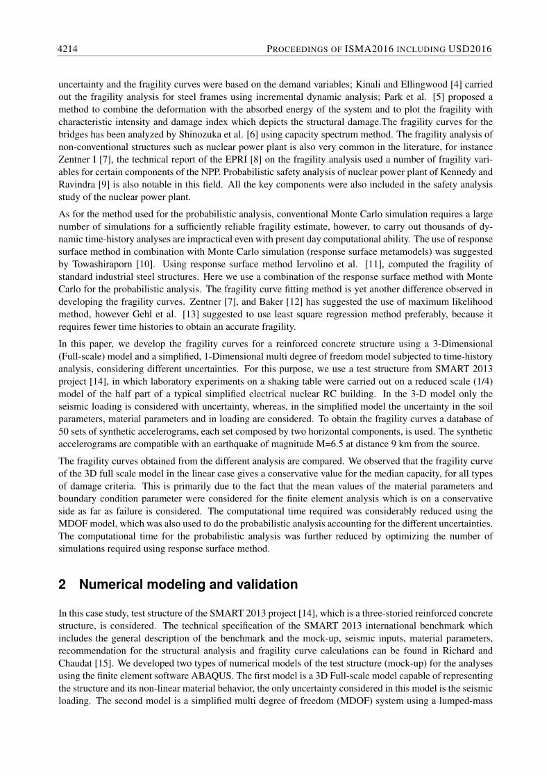
Modal analysis is performed to calibrate the linear elastic characterization of the numerical model of thestructure. The eigenvalues extraction is done by using the Lanczos eigensolver and Rayleigh damping of5%. Different boundary conditions are considered and only the case with the shaking table along with thestructure and additional masses is presented here. This case assumes that the anchorage points between theactuators and the shaking table are fixed. The first three natural frequencies of both models are listed inTable 1.

USD - CIVIL & WIND APPLICATIONS 4215

Mode Experiment Full − scale MDOF

1 6.28 5.99 6.032 7.86 9.28 10.793 16.50 19.84 35.05

Table 1: Comparison of the natural frequencies of the structure

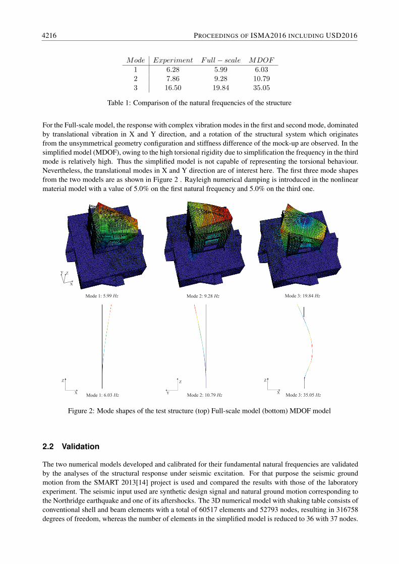
For the Full-scale model, the response with complex vibration modes in the first and second mode, dominatedby translational vibration in X and Y direction, and a rotation of the structural system which originatesfrom the unsymmetrical geometry configuration and stiffness difference of the mock-up are observed. In thesimplified model (MDOF), owing to the high torsional rigidity due to simplification the frequency in the thirdmode is relatively high. Thus the simplified model is not capable of representing the torsional behaviour.Nevertheless, the translational modes in X and Y direction are of interest here. The first three mode shapesfrom the two models are as shown in Figure 2 . Rayleigh numerical damping is introduced in the nonlinearmaterial model with a value of 5.0% on the first natural frequency and 5.0% on the third one.

Mode 1: 5.99 Hz Mode 2: 9.28 Hz Mode 3: 19.84 Hz

Z

X

ZY

Mode 1: 6.03 Hz Mode 2: 10.79 Hz Mode 3: 35.05 HzX

Z

Y

Z

X

Figure 2: Mode shapes of the test structure (top) Full-scale model (bottom) MDOF model

2.2 Validation

The two numerical models developed and calibrated for their fundamental natural frequencies are validatedby the analyses of the structural response under seismic excitation. For that purpose the seismic groundmotion from the SMART 2013[14] project is used and compared the results with those of the laboratoryexperiment. The seismic input used are synthetic design signal and natural ground motion corresponding tothe Northridge earthquake and one of its aftershocks. The 3D numerical model with shaking table consists ofconventional shell and beam elements with a total of 60517 elements and 52793 nodes, resulting in 316758degrees of freedom, whereas the number of elements in the simplified model is reduced to 36 with 37 nodes.


The linear behaviour of the models are validated using the lower intensity ground motion (PGA of 0.1g) andfor the nonlinear behavior using higher intensity ground motions (PGA of 0.2g to 1g). The implicit solver ofthe ABAQUS is used for the dynamic analysis.

Linear response of the models are obtained from the structural response under de excitation using groundmotions represented by synthetic white noise and scaled design signal of PGA as high as 1 g as specifiedin [15]. The displacement response and acceleration response at several points (A,B,C and D as shown inFigure 1(d) on the structure are compared for the Full-scale model. In the case of the simplified model the topstory response is considered. The response obtained as displacement time history and corresponding to thescaled design signal is as shown in Figure 3 (a). The displacement Fourier spectra as well as the displacementresponse spectra are also shown in Figure 3 (b) and (c) respectively. The response spectra shows a closematch with the experimental results. Overall, the comparisons of displacement in the linear domain arereasonably consistent with the experiment. Some discrepancies observed are due to the simplification of themodel, which is unavoidable.

(a) (b)

(c)

Spec

tral d

ispl

acem

ent

Dis

plac

emen

t [m

m]

Am

plitu

de (d

ispl

acem

ent)

Time [s]

Period [s]

Frequency [Hz]

Figure 3: Comparison of the linear response of MDOF and Full-scale model with experiment

Nonlinear response The nonlinear response is obtained only for the full-scale model, the material nonlin-earity using constitutive law with softening is represented by the concrete damage plasticity (CDP) modelprovided by ABAQUS. The implicit solver successfully finds solutions for all the ground motions in theexperiment including the Northridge earthquake(PGA 1g). Plastic strain under the strong shaking of PGA of1g is concentrated on the walls at the ground level and at the intersection of the walls at the foundation level.A small amount of plastic strain is observed at the window openings of each floor. As seen from the Figure 4,for lower PGA of 0.2 g (design signal) the displacement response in X and Y direction is comparable withthe experiment. But for higher PGA (1g) the displacement and acceleration amplitudes are underestimatedcompared with those of the experiment. These deviations are maybe due to the unrealistic connection withthe test structure and very stiff shaking table. The assumption of fixed connection between the shaking tableand the test structure is made in the numerical analysis. However, in the actual experiment the connection


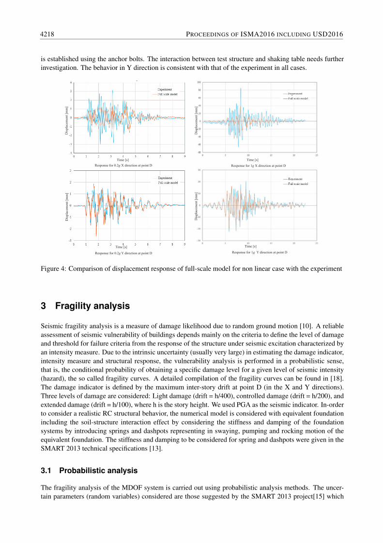
is established using the anchor bolts. The interaction between test structure and shaking table needs furtherinvestigation. The behavior in Y direction is consistent with that of the experiment in all cases.

Response for 1g X direction at point DResponse for 0.2g X direction at point D

Response for 0.2g Y direction at point D Response for 1g Y direction at point D

Dis

plac

emen

t [m

m]

Time [s]

Dis

plac

emen

t [m

m]

Time [s]

Dis

plac

emen

t [m

m]

Time [s]

Dis

plac

emen

t [m

m]

Time [s]

Figure 4: Comparison of displacement response of full-scale model for non linear case with the experiment

3 Fragility analysis

Seismic fragility analysis is a measure of damage likelihood due to random ground motion [10]. A reliableassessment of seismic vulnerability of buildings depends mainly on the criteria to define the level of damageand threshold for failure criteria from the response of the structure under seismic excitation characterized byan intensity measure. Due to the intrinsic uncertainty (usually very large) in estimating the damage indicator,intensity measure and structural response, the vulnerability analysis is performed in a probabilistic sense,that is, the conditional probability of obtaining a specific damage level for a given level of seismic intensity(hazard), the so called fragility curves. A detailed compilation of the fragility curves can be found in [18].The damage indicator is defined by the maximum inter-story drift at point D (in the X and Y directions).Three levels of damage are considered: Light damage (drift = h/400), controlled damage (drift = h/200), andextended damage (drift = h/100), where h is the story height. We used PGA as the seismic indicator. In-orderto consider a realistic RC structural behavior, the numerical model is considered with equivalent foundationincluding the soil-structure interaction effect by considering the stiffness and damping of the foundationsystems by introducing springs and dashpots representing in swaying, pumping and rocking motion of theequivalent foundation. The stiffness and damping to be considered for spring and dashpots were given in theSMART 2013 technical specifications [13].

3.1 Probabilistic analysis

The fragility analysis of the MDOF system is carried out using probabilistic analysis methods. The uncer-tain parameters (random variables) considered are those suggested by the SMART 2013 project[15] which


includes the foundation stiffness and damping, structural damping ratio, and concrete strength. Lognormaland normal distribution of the properties are chosen. A software program NESSUS [19] in combination withABAQUS is used for the probabilistic analysis. The use of conventional Monte Carlo requires very largenumber of structural time-history simulation. To overcome this, we used response surface methodology forthe probabilistic structural analysis. A combination of the response surface method (RSM) and conventionalMonte-carlo simulations are used for the whole probabilistic analysis. The method is adopted from the PhDthesis of Towashiraporn [10].

3.1.1 Response surface method and structural response

RSM is the process of developing a functional relationship between random input variables (RIV) and ran-dom output variables (ROV), also referred to as responses. Using Latin Hypercube Sampling (LHS), whichdivides the sampling space into sectors of equal probability of occurrence and selects one realization fromeach sector, the sampling of the random input variables are done. Design of experiments are carried asan initial step of the RSM, Central Composite Design (CCD) is the most commonly used experimentaldesign [20]. NESSUS, however offers two options to carry out the response surface method, using responsesurface tool kit capable of generating efficient designs for experiments using spacing-optimized Latin Hyper-cube Sampling and the other option is to use CCD, or Box-Behnken design. We have used the former option,the number of samples used is as suggested by the user’s manual. At these points, the structural responsesare computed in order to use the obtained training data to develop a functional relationship between inputand output variables. This was done for 50 different time histories and with 70 samples for each time-history.

The result obtained is a random output variable, the relation between the RIV and ROV are represented usingthe response surfaces, Polynomial regression is used to fit the response. For the polynomial regression model,the function of the response surface is approximated by a polynomial function. The higher the polynomialdegree, the more computations are required. To decrease computational effort, the polynomial function iscommonly assumed to be of first or second order. We have used the second order polynomial given by,

y = β0 +k∑i=1

βixi +k∑i=1

βiix2i +

∑i<

∑j

βijxixj + ε (1)

where y is the ROV, xi, xj are the RIV, β0 βi are the regression coefficients, i represents the expected changein response y per unit change in xi when all remaining independent variables xj (j i) are held constant [20].k denotes the number of input variables, and ε the experimental error which describes the difference of thefunctional values y from the response values of the analysis. A polynomial fitted response surface is shownin Figure 5 which corresponds to the 1.7g PGA. It is inferred that the response of the structure lies within thissurface and therefore the surfaces are further evaluated using Monte Carlo method for each PGA, giving theprobability of failure corresponding to each peak ground acceleration. The fragility curves are then plottedusing Maximum likelihood method and linear regression in order to fit the curve as explained in the followingsections.

3.2 Development of fragility curves

For the determination of fragility curves, lognormal fragility model is chosen, hence the fragility curves aredefined by two parameters, the median capacity Am, and the lognormal standard deviation β, for a seismicintensity θ.The fragility curve is generally modeled using a lognormal cumulative distribution function, achoice supported by studies in the past in different fields for e.g. Ellingwood [21], Singhal and Kiremidjian[22], Shinozuka et al.[23]. Therefore, the fragility curve is mathematically described as given in Equation 2

Pf (θ) = Φ

(ln(θ/Am)

β

)(2)


Figure 5: Response surface corresponding to a PGA of 1.7g

where φ is the standard normal probability distribution function θ is the seismic intensity, which in here indi-cates PGA, is the median capacity expressed in terms of θ, β is the lognormal standard deviation.The mediancapacity and lognormal standard deviation can be determined either by regression analysis or maximumlikelihood method [23], [7].

3.2.1 Fullscale model

In the case of the 3D full scale model, the parameter with uncertainty is considered only for the seismicloading. The material parameters are considered to be with their mean value in the numerical model. In thiscase, for the determination of the fragility curves, we used linear regression method, as suggested by [15]in the SMART 2013 project for the determination of fragility curves for various damage level the simplemethod. The obtained inter story drift from both linear and nonlinear dynamic analyses of the numericalmodel is accounted here. The empirical relationship obtained from this analyses is a linear equation, givenby

ln(D) = a+ b ln θ (3)

here a and b are the coefficients from the regression analysis. The value of Am is then computed usingEquation 4, Dd is the critical threshold of damage indicator

ln(Am) =ln(Dd)− a

b(4)

Lognormal standard deviation β is computed from the dispersion of data from Equation 4 and given by

β2 =1

N

N∑i=1

[ln(Di)− ln(D)]2 (5)

The fragility curves shown in the Figure 6 are obtained using linear and nonlinear dynamic analysis. Thedamage predictor is calculated using the linear regression as shown on the left in the Figure 6. The predictorline in linear and nonlinear case are different for X and Y direction, in the X direction the linear case predicts


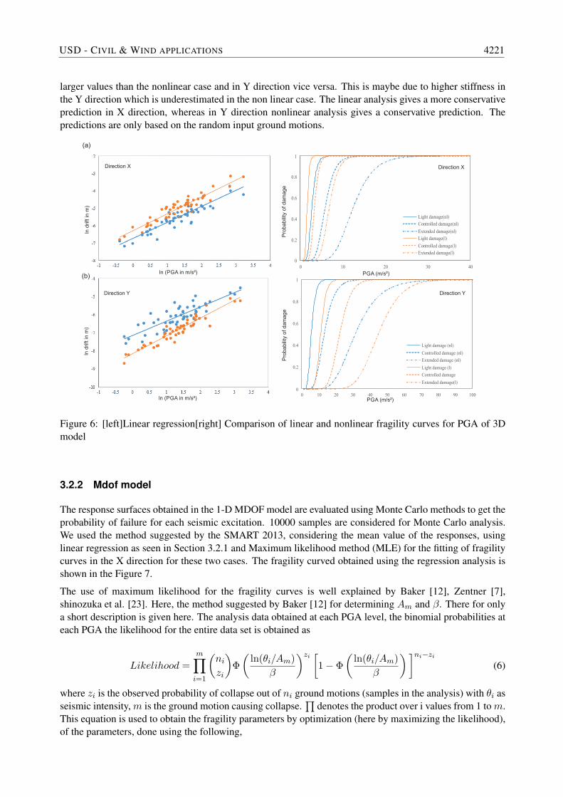
larger values than the nonlinear case and in Y direction vice versa. This is maybe due to higher stiffness inthe Y direction which is underestimated in the non linear case. The linear analysis gives a more conservativeprediction in X direction, whereas in Y direction nonlinear analysis gives a conservative prediction. Thepredictions are only based on the random input ground motions.

0

0.2

0.4

0.6

0.8

1

0 10 20 30 40

Light damage(nl)Controlled damage(nl)Extended damage(nl)Light damage(l)Controlled damage(l)Extended damage(l)

ln (PGA in m/s²)

ln d

rift i

n m

)

Prob

abilit

y of

dam

age

Prob

abilit

y of

dam

age

Direction X

Direction Y

ln (PGA in m/s²)

ln d

rift i

n m

)

(a)

(b)

0

0.2

0.4

0.6

0.8

1

0 10 20 30 40 50 60 70 80 90 100

Light damage (nl)Controlled damage (nl)Extended damage (nl)Light damage (l)Controlled damageExtended damage(l)

PGA (m/s²)

PGA (m/s²)

Direction X

Direction Y

Figure 6: [left]Linear regression[right] Comparison of linear and nonlinear fragility curves for PGA of 3Dmodel

3.2.2 Mdof model

The response surfaces obtained in the 1-D MDOF model are evaluated using Monte Carlo methods to get theprobability of failure for each seismic excitation. 10000 samples are considered for Monte Carlo analysis.We used the method suggested by the SMART 2013, considering the mean value of the responses, usinglinear regression as seen in Section 3.2.1 and Maximum likelihood method (MLE) for the fitting of fragilitycurves in the X direction for these two cases. The fragility curved obtained using the regression analysis isshown in the Figure 7.

The use of maximum likelihood for the fragility curves is well explained by Baker [12], Zentner [7],shinozuka et al. [23]. Here, the method suggested by Baker [12] for determining Am and β. There for onlya short description is given here. The analysis data obtained at each PGA level, the binomial probabilities ateach PGA the likelihood for the entire data set is obtained as

Likelihood =

m∏i=1

(nizi

)Φ

(ln(θi/Am)

β

)zi[1− Φ

(ln(θi/Am)

β

)]ni−zi

(6)

where zi is the observed probability of collapse out of ni ground motions (samples in the analysis) with θi asseismic intensity, m is the ground motion causing collapse.

∏denotes the product over i values from 1 tom.

This equation is used to obtain the fragility parameters by optimization (here by maximizing the likelihood),of the parameters, done using the following,


ln (PGA in m/s²)

ln d

rift i

n m

)

Prob

abili

ty o

f dam

age

Direction X

PGA (m/s²)

Light damageControlled damageExtended damage

Figure 7: [left]Linear regression[right] fragility curves for MDOF model

{θ, β}

= argmaxθ,β

m∑i=1

{ln

(nizi

)+ ln Φ

(ln(θi/Am)

β

)(ni − zi) ln

[1− Φ

(ln(θi/Am)

β

)]}(7)

The fragility curve fitting and the fitted curves for the MDOF model is as shown in the Figure 8. A com-parison of the fragility curves obtained from the linear and nonlinear case of the full-scale model with theMDOF model using two methods are as shown in the Table 2. From our observations, it is evident that,the fragility curves obtained using the linear case of the full-scale model is very conservative compared tothe simplified model in X direction. The point D on the structure and on the fullscale model encounters themaximum displacement due to asymmetric plan of the structure, this torsional effect is however neglected inthe MDOF model and the deflection is measured at the center of mass at the top floor. Therefore the behaviorof the MDOF can be justified.

Prob

abili

ty o

f dam

age

PGA (m/s²)

Prob

abili

ty o

f dam

age

PGA (m/s²)

Fraction causing collapseFitted curve

Light damage (MLE)Controlled damage (MLE)

Extended damage (MLE)

Figure 8: [left]MLE fitting[right] Fitted fragility curves using MLE for MDOF model

ModelMedian capacity Am β

Light damage Controlled damage Extended DamageFullscale linear 1.62 3.32 6.79 0.25Fullscale nonlinear 2.74 5.83 12.41 0.31MDOF (LR) 4.77 8.46 14.99 0.33MDOF(MLE) 4.0 7.6 12.01 0.21

Table 2: Comparison of the mean value and standard deviation of the fragility curves in X direction

The behavior of the fragility curves for 10000 samples, developed using MLE is very steep, with maximum


standard deviation of 0.21. It may be also noted that the standard deviation for the fragility curves in con-trolled damage and extended damage is 0.1. In the ground motion considered, there is an abrupt jump fromPGA 1.03g to PGA 1.69g. The total collapse (extended damage) of the structure occurs in all cases at PGAequal to and higher than 1.69g. The fragility curves for the MDOF model developed using the methodssuggested by SMART 2013 using the mean values of the responses, the median capacity is higher comparedto other methods. Here the mean values are obtained for each ground motion from a set of 70 samples, thatis from the random output variable of the response surface method. The MDOF model is only capable ofrepresenting the linear behaviour of the structure. It may be also noted that the 3D model only represents therandomness in the ground motion excitation, the other uncertainties are not considered, rather the mean valueof the parameters are used for obtaining the structural response. This leads to a more conservative behavior.

4 Discussions and conclusions

Probabilistic safety/risk analysis has become the most commonly used approach for the evaluation of seismicrisk in nuclear power industry. The fragility curves are the major elements of the this type of analysis. In thispaper, we have developed the fragility curves for a reinforced concrete test structure, which is a representativeelectrical building of a nuclear facility that was tested in SMART 2013 [14] project. Two numerical modelsare used, the first one is a one-to-one scaled three-dimensional model of the structure accounting for randomseismic input and the a one-dimensional simplified model with beam elements and lumped masses whichaccounts uncertainty in ground motion, material and structural properties. To obtain the fragility curves adatabase of 50 sets of synthetic accelerograms, each set composed by two horizontal components, is used.The synthetic accelerograms are compatible with an earthquake of magnitude M=6.5 at distance 9 km fromthe source. The use of response surface method instead of conventional Monte Carlo method, reduces thecomputational time drastically as less number of samples are required for the structural simulation.

Fragility curves are estimated using the method suggested by the SMART 2013 project which is a linearregression for the fullscale model. For the simplified model, apart from the regression we also used themaximum likelihood method. A comparison of the fragility curves for full scale model and the MDOF modelin x-direction shows that the fragility curves obtained from the fullscale model in the linear analysis gives amore conservative design compared to the simplified model. This may be due to the assumptions of usingonly the mean values of the material and boundary condition parameters without uncertainties in the finiteelement analysis, which is on a conservative side. The computational time required was considerably reducedusing the MDOF model, which was also used to do the probabilistic analysis accounting for the differentuncertainties. The computational effort for the probabilistic analysis was further reduced by optimizing thenumber of simulations required using response surface method.

Acknowledgements

We would like to thank the organizers of SMART2013 for the opportunity to participate in the benchmarkproject and swissnuclear for the financial support to carry out a part of this work. The first author alsogratefully acknowledge the financial support from BMWi (Bundesministerium fuer Wirtschaft und Energie)and GRS(Gesellschaft fuer Anlagen- und Reaktorsicherheit) gGMBH for the project number 1501503.

References

[1] E. Dumova-Jovanoska, Fragility curves for reinforced concrete structures in skopje (macedonia) region,Soil Dynamics and Earthquake Engineering, Vol. 19, No. 6, (2000), pp. 455–466.


[2] B. R. Ellingwood, O. C. Celik, K. Kinali, Fragility assessment of building structural systems in mid-america, Earthquake Engineering & Structural Dynamics, Vol. 36, No. 13, (2007), pp. 1935–1952.

[3] P. Gardoni, A. Der Kiureghian, K. Mosalam, Probabilistic capacity models and fragility estimates forreinforced concrete columns based on experimental observations, Journal of Engineering Mechanics,Vol. 128, No. 10, (2002), pp. 1024–1038.

[4] K. Kinali, B. R. Ellingwood, Seismic fragility assessment of steel frames for consequence-based engi-neering: A case study for memphis, tn, Engineering structures, Vol. 29, No. 6, (2007), pp. 1115–1127.

[5] Y.-J. Park, A. H.-S. Ang, Y. K. Wen, Seismic damage analysis of reinforced concrete buildings, Journalof Structural Engineering, Vol. 111, No. 4, (1985), pp. 740–757.

[6] M. Shinozuka, M. Q. Feng, H.-K. Kim, S.-H. Kim, Nonlinear static procedure for fragility curvedevelopment, Journal of engineering mechanics.

[7] I. Zentner, Numerical computation of fragility curves for npp equipment, Nuclear Engineering andDesign, Vol. 240, No. 6, (2010), pp. 1614–1621.

[8] J. W. Reed, R. P. Kennedy, Methodology for developing seismic fragilities, Tech. rep., EPRI (1994).

[9] R. Kennedy, M. Ravindra, Seismic fragilities for nuclear power plant risk studies, Nuclear Engineeringand Design, Vol. 79, No. 1, (1984), pp. 47–68.

[10] P. Towashiraporn, Building seismic fragilities using response surface metamodels, Ph.D. thesis, GeorgiaInstitute of Technology ((2004)).

[11] I. Iervolino, G. Fabbrocino, G. Manfredi, Fragility of standard industrial structures by a responsesurface based method, Journal of Earthquake Engineering, Vol. 8, No. 06, (2004), pp. 927–945.

[12] J. W. Baker, Efficient analytical fragility function fitting using dynamic structural analysis, EarthquakeSpectra, Vol. 31, No. 1, (2015), pp. 579–599.

[13] P. Gehl, J. Douglas, D. M. Seyedi, Influence of the number of dynamic analyses on the accuracy ofstructural response estimates, Earthquake Spectra, Vol. 31, No. 1, (2015), pp. 97–113.

[14] Seismic desing and best-estimate methods assesment for reinforced concrete buildings subjected totorsion and non-linear effects, http://www.smart2013.eu/, accessed: 2010-09-30.

[15] B. Richard, T. Chaudat, Presentation of the smart 2013 international benchmark, CEA/DEN TechnicalReport. DEN/DANS/DM2S/SEMT/EMSI/ST/12-017/H.

[16] L. A. Dalguer, P. Renault, S. Churilov, C. Butenweg, Evaluation of fragility curves for a three-storeyreinforced concrete mock-up of smart 2013 project, Proceedings of Structural Mechanics and ReactorTechnology 23 Conference.

[17] L. A. Dalguer, S. Churilov, C. Butenweg, P. Renault, J. An, Dynamic analysis of a reinforced concreteelectrical nuclear building of smart 2013 project subjected to earth-quake excitation using abaqus,Proceedings of the SMART2014 Workshop, Paris, France,.

[18] G. Calvi, R. Pinho, G. Magenes, J. Bommer, L. Restrepo-Velez, H. Crowley, Development of seismicvulnerability assessment methodologies over the past 30 years, ISET journal of Earthquake Technology,Vol. 43, No. 3, (2006), pp. 75–104.

[19] B. H. Thacker, D. S. Riha, S. H. Fitch, L. J. Huyse, J. B. Pleming, Probabilistic engineering analysisusing the nessus software, Structural Safety, Vol. 28, No. 1, (2006), pp. 83–107.


[20] R. H. Myers, D. C. Montgomery, Anderson-Cook, C. M, Response surface methodology: process andproduct optimization using designed experiments, John Wiley & Sons (2016).

[21] B. Ellingwood, Validation studies of seismic pras, Nuclear Engineering and Design, Vol. 123, No. 2-3,(1990), pp. 189–196.

[22] A. Singhal, A. S. Kiremidjian, Method for probabilistic evaluation of seismic structural damage, Jour-nal of Structural Engineering, Vol. 122, No. 12, (1996), pp. 1459–1467.

[23] M. Shinozuka, M. Q. Feng, J. Lee, T. Naganuma, Statistical analysis of fragility curves, Journal ofEngineering Mechanics, Vol. 126, No. 12, (2000), pp. 1224–1231.


seismic fragility analysis of a non-conventional...

Documents