Cyclic1D

Seismic Ground Response

Version 1.4

User’s Manual

Ahmed Elgamal, Zhaohui Yang, and Jinchi Lu

University of California, San Diego

Department of Structural Engineering May 2015

The references for Cyclic1D are: Elgamal, A., Yang, Z., and Lu, J. (2006). “Cyclic1D: A Computer Program for Seismic Ground

Response,” Report No. SSRP-06/05, Department of Structural Engineering, University of California, San Diego, La Jolla, CA.

Yang, Z., Lu, J., and Elgamal, A. (2004). "A Web-Based Platform for Computer Simulation of Seismic Ground Response." Advances in Engineering Software, 35(5), 249-259.

2

Table of Contents

INTRODUCTION ......................................................................................................................................... 3 

EXECUTION OF CYCLIC1D: HELPFUL HINTS ............................................................................................. 4 SYSTEM REQUIREMENTS ........................................................................................................................... 5 INSTALLATION ............................................................................................................................................. 5 

DEFINITION OF MODEL PROFILE ......................................................................................................... 6 

SOIL STRATUM ........................................................................................................................................... 6 INPUT MOTION ............................................................................................................................................ 8 SOIL PROPERTIES ...................................................................................................................................... 9 

Theory.................................................................................................................................................... 9 Element Input ..................................................................................................................................... 10 Predefined materials ......................................................................................................................... 10 User-defined materials ...................................................................................................................... 11 

User Defined Clay/Rock Strata with No Pore-Pressure Effects ............................................................... 11 User Defined Granular Soil with No Pore-Pressure Effects ...................................................................... 12 User Defined Saturated Granular Strata with Pore-Pressure Effects ...................................................... 13 

ADDITIONAL VISCOUS DAMPING .............................................................................................................. 16 STEP-BY-STEP TIME INTEGRATION .......................................................................................................... 17 

RUNNING THE ANALYSIS ..................................................................................................................... 18 

RESPONSE AT A LOCATION ...................................................................................................................... 18 RESPONSE PROFILE ................................................................................................................................. 19 REPORT GENERATOR .............................................................................................................................. 20 

ACKNOWLEDGMENTS ........................................................................................................................... 22 

REFERENCES ........................................................................................................................................... 23 

APPENDIX I: CYCLIC1D-RELATED REFERENCES ......................................................................... 25 

APPENDIX II: BUILT-IN SOIL MATERIALS IN CYCLIC1D: PARAMETERS AND UNITS ......... 27 

3

Introduction Cyclic1D is a nonlinear Finite Element program for one-dimensional (1D) lateral dynamic site-response simulations. The program operates in the time domain, allowing for linear (Hughes 1987) and nonlinear studies. Nonlinearity is simulated by incremental plasticity models to allow for modeling permanent deformation and for generation of hysteretic damping. For analysis of dry as well as saturated strata, the finite elements are defined within a coupled solid-fluid (u-p) formulation (Chan 1988, Ziekiewicz et al. 1990). Dry and/or saturated soil profiles may be studied. In saturated cohesionless soil strata, liquefaction and its effects on ground acceleration and permanent deformation are modeled. In this regard, the user may wish to explore the response of a level ground site, or conversely to investigate the response of a mildly-inclined infinite-slope site. The Microsoft Windows-based interface allows for: 1) convenient pre-processing (i.e., preparation of input data file), 2) initiation and execution of the computations, 3) display of the response (output), and 4) generation of an output report with the desired figures and relevant information. This interface is designed for simplicity, and is intended to be intuitive and self-explanatory.

4

Execution of Cyclic1D: Helpful Hints 1) Cyclic1D operates in SI units. 2) Start with the simplest possible model of the scenario you wish to study. As you gain confidence in the results, gradually proceed towards more elaborate simulations. If you are a new user, consider running a simple case using one of the U-clay-rock models, and specify “Linear run”. Under an earthquake excitation (with rigid base specified), you should observe the fundamental resonance at the frequency of f1 = Vs/4H (in Hz), where Vs is the shear wave velocity and H is the stratum height (for example, try perhaps a Vs = 200 m/sec and H = 50 m, with 50 elements for example, and check figures of Spectral amplification of acceleration relative to base motion). In this simple case, higher resonances should appear at 3f1, 5 f1, 7 f1 and so forth. Note that these resonant responses will become more pronounced as you reduce the specified viscous damping. The actual numerical resonant frequencies should approach the above theoretical values as the specified number of elements modeling the stratum increases, and as the base excitation file time-step decreases (and also as the duration of base excitation increases, see Chopra 2000). For shear beam resonance, see Elgamal (1991). 3) The smaller, the element height, the higher the frequency content that the model is able to simulate. For traditional site response calculations, seismic excitation is usually primarily rich in frequencies of up to 15 Hz or thereabout. As you finalize your work, it might be worthwhile to run your model with a finer mesh (i.e., more elements), and to check that the results are of acceptable accuracy (i.e., the higher frequency response is becoming stable and is not changing significantly). It is suggested to undertake this step only after you have verified that all modeling parameters are in good order, and that the resulting response is logical (in order to save time and effort). As a guideline (for linear analysis), the maximum frequency Fmax that an element of shear wave velocity Vs, and height h can transmit is Fmax = (Vs/h) / 4.0. 3) Make use of the available help buttons in the Windows Interface for additional clarifications.

5

System Requirements Cyclic1D runs on PC compatible systems using either Windows XP, Windows 7 or 8. The system should have a minimum hardware configuration appropriate to the particular operating system. Installation After downloading the Cyclic1D installation file, double-click on the icon and the installation procedure will start. Once installed, the default case in Cyclic1D is a good way to go through the steps involved in conducting a Cyclic1D analysis. The interface will allow the user to prepare and save an input file, to run the analysis, and to display the response. A “Report Generator” facility allows users to save all or selected input parameters and response figures.

6

Definition of Model Profile Soil Stratum Soil Profile Height The Soil Profile Height is in meters. Number of Elements The Number of Elements can be chosen between 10 and 2000. Water Table Depth The Water Table Depth refers to the depth below ground surface.(e .g., 0.0 corresponds to a fully saturated soil profile, 1.0 is 1m below ground surface). Dry sites should specify water table depth to be equal to the entire model depth. Inclination Angle The Inclination Angle is in degrees (Zero degree represents level ground). For mildly-inclined infinite-slopes, suggested values are from 0 to 10 degrees. Bedrock A rigid base may be specified (corresponds to an infinitely rigid rock base). In this case, the base input excitation is actually the total acceleration occurring at the model base. For situations other than the rigid base, properties of bedrock are as follows:

Bedrock type Shear wave velocity1 (m/s) Mass density (kg/m3)

Soft Rock 700 2500

Rock 1100 2500

Hard Rock 1600 2500

U-Rock (User-defined) 2 (User-defined) 3 (User-defined) 4

1. Shear wave velocities for rocks are based on International Code Council (1998). 2000 International Building Code (Final Draft).

2. There are two options for a user to define own rock: one is to use the same properties as the soil column at the bottom element; the other is that the properties are defined by the user.

3. User-defined shear wave velocity in m/s (suggested values between 100 and 6000).

4. User-defined mass density in kg/m3 (suggested values between 1300 and 2500

kg/m3). Other than the rigid base scenario, the specified input motion acceleration file is considered to be the “incident” motion component only. As such, the program computes the total motion at the specified stratum-rock interface (i.e., sum of the incident and reflected waves). Incident motion files may sometimes be obtained by: 1) Using a recorded rock-outcrop acceleration file with the amplitudes scaled to ½ of the recorded values (assuming the rock outcrop to be essentially “Rigid”, incident motion is ½

7

of the recorded ground surface motion), 2) Using an appropriate program that allows de-convolution, (e.g., the well-known program SHAKE, Schnabel et al. 1972), starting with a ground surface rock-outcrop motion and computing the motion at the desired base-input depth. From the SHAKE result, define the incident motion at the desired depth for use in Cyclic1D. This incident motion (upward propagating waves) is ½ of the SHAKE-computed so-called “outcrop motion” at the desired depth, or 3) Starting at the surface with a recorded ground surface acceleration record and attempting to de-convolve this motion using SHAKE for instance (as described above). This approach has been known to be problematic and is not recommended.

8

Input Motion Motion Type If "Bedrock" is assumed "Rigid", the input motion selected below is total motion; If "Bedrock" is not assumed "Rigid", input motion is treated as a rock outcrop motion (i.e, as the incident component of seismic excitation).

A user-specified input motion can be defined by selecting “U-Shake”. The input motion file to be defined should consist of two columns, Time (seconds) and Acceleration (g), delimited by SPACE(S).

Below is an example of a user-defined input motion file:

0.00 0.000 0.02 0.005 0.04 0.030 0.06 -0.022 ... .…..... 19.98 0.004 20.00 0.000 Note that the user-defined input motion file must be placed in the subfolder “motions/”. (This subfolder also contains all provided built-in input motion files). Scale Factor The amplitude of the input motion is multiplied by the Scale Factor. The Scale Factor may be positive or negative. Frequency The Frequency (in Hz) has to be specified if harmonic “Sinusoidal Motion” is chosen Number of Cycles The Number of Cycles has to be specified if “Sinusoidal Motion” is chosen.

9

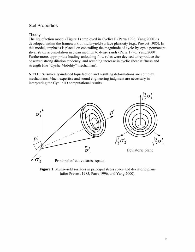
Soil Properties Theory The liquefaction model (Figure 1) employed in Cyclic1D (Parra 1996, Yang 2000) is developed within the framework of multi-yield-surface plasticity (e.g., Prevost 1985). In this model, emphasis is placed on controlling the magnitude of cycle-by-cycle permanent shear strain accumulation in clean medium to dense sands (Parra 1996, Yang 2000). Furthermore, appropriate loading-unloading flow rules were devised to reproduce the observed strong dilation tendency, and resulting increase in cyclic shear stiffness and strength (the “Cyclic Mobility” mechanism). NOTE: Seismically-induced liquefaction and resulting deformations are complex mechanisms. Much expertise and sound engineering judgment are necessary in interpreting the Cyclic1D computational results.

1 2

3

2 2

3 3 2

3

1

2 3

0p

p

Principal effective stress space

Deviatoric plane

Figure 1: Multi-yield surfaces in principal stress space and deviatoric plane

(after Prevost 1985, Parra 1996, and Yang 2000).

10

Element Input Enter element numbers (and/or ranges) associated with each material, separated by commas. For example, 1-3,4,5,6-8. Element numbering is from the top down (i.e., Element 1 is at the surface). Predefined materials There are15 predefined materials. Basic model parameter values for these materials are listed below.

Cohesionless Soil

Shear wave velocity at

10m depth1,2

(m/s)

Friction angle3

(degrees)

Poisson's ratio4

Permeability coeff.5 (m/s)

Mass density6 (kg/m3)

Loose, silt permeability 185 29 0.4 1.0E-07 1700

Loose, sand permeability 185 29 0.4 6.6E-05 1700

Loose, gravel permeability 185 29 0.4 1.0E-02 1700

Medium, silt permeability 205 31.5 0.4 1.0E-07 1900

Medium, sand permeability

205 31.5 0.4 6.6E-05 1900

Medium, gravel permeability

205 31.5 0.4 1.0E-02 1900

Medium-dense, silt permeability

225 35 0.4 1.0E-07 2000

Medium-dense, sand permeability

225 35 0.4 6.6E-05 2000

Medium-dense, gravel permeability

225 35 0.4 1.0E-02 2000

Dense, silt permeability 255 40 0.4 1.0E-07 2100

Dense, sand permeability 255 40 0.4 6.6E-05 2100

Dense, gravel permeability

255 40 0.4 1.0E-02 2100

Cohesive Soil Shear wave

velocity (m/s)

Undrained shear

strength7 (kPa)

Poisson's ratio

Permeability coeff.5 (m/s)

Mass density6 (kg/m3)

Soft 100 18.0 0.4 1.0E-09 1300

Medium 200 37.0 0.4 1.0E-09 1500

Stiff 300 75.0 0.4 1.0E-09 1800

11

1. Shear wave velocity of cohesionless soils varies approximately in proportion to (pm)1/4 where pm is effective mean confinement.

2. Shear wave velocities for cohesionless soils are based on the empirical formula of Seed and Idriss (1970).

3. Friction angles for cohesionless soils are based on Table 7.4 (p.425) of Das, B.M. (1983).

4. Poisson’s ratio is used for calculation of initial lateral confinement (K0).

5. Permeability values are based on Figure 7.6 (p.210) of Holtz and Kovacs (1981).

6. Mass density is based on Table 1.4 (p.10) of Das (1995).

7. Undrained shear strength for cohesive soils are based on Table 7.5 (p.442) of Das (1983).

User-defined materials There are 30 user-defined materials including 10 clay/rock materials with properties independent of confinement variation and 10 sandy materials with confinement- dependent material properties. Some user-defined materials do not take into account dynamic pore pressure generation effects. Therefore, this class of materials is suitable for soil layers that are not susceptible to significant pore pressure variation during earthquake excitation. To define the parameters of a user-defined material, click on the button associated with that material and fill in the pop-up window. User Defined Clay/Rock Strata with No Pore-Pressure Effects

Non-liquefiable clayey/rock strata with shear response properties independent of confinement variation can be defined by specifying the following parameters (Figure 2):

1. Mass density in kg/m3 (suggested range of values between 1000 and 3000 kg/m3).

2. Shear wave velocity in m/s (suggested range of values between 10 and 6000m/s).

3. Initial lateral/vertical stress ratio (also known as coefficient of lateral earth pressure at rest K0, suggested range of values between 0.1 and 0.9. In the program, K0 is related to Poisson’s ratio by the following relation: )1(/0 v v K .

4. Shear strength in kPa (suggested range of values between 10 and 200000 kPa).

5. Peak shear strain in % (suggested range of values between 0.001% and 20%).

6. Number of yield surfaces (NYS). Suggested range of values is 0 and 30.

12

In particular, NYS=0 dictates an elastic response (Parameters 4 and 5 are ignored, see Figure 2), NYS=1 indicates an elastic-perfectly plastic response (Parameter 5 is ignored, see Figure 2 below).

Shearstress

Shearstrength

Peak shearstrain

Shearstrain

Number of yieldsurfaces = 5

Shear modulus =Mass density x

(Shear wave velocity)2

Shearstress

Shearstrain

Number of yieldsurfaces = 0

Shear modulus =Mass density x

(Shear wave velocity)2

Shearstress

Shearstrength

Shearstrain

Number of yieldsurfaces = 1

Shear modulus =Mass density x

(Shear wave velocity)2

Figure 2: Soil Backbone curve and yield surfaces User Defined Granular Soil with No Pore-Pressure Effects Granular Soil (e.g., Sands, gravels, non-plastic silts) with confinement-dependent shear response not susceptible to significant pore pressure variations can be defined by specifying the following parameters (see Figure 2):

Note: All parameters shown in Figure 2 are defined at the reference mean confinement pr 1. Mass density in kg/m3 (suggested range of values between 1000 and 3000 kg/m3).

2. Reference mean confinement (pr) in kPa. This is the confinement level at which soil appropriate soil properties below (see also Figure 2) are defined.

13

3. Reference shear wave velocity (Vsr) in m/s (suggested range between 10 and 6000m/s). This Vsr corresponds to the Reference mean confinement pr.

4. Confinement dependence coefficient (n). Shear wave velocity Vs varies with

confinement p in this form 2/)/( nrsrs pp V V .

5. Initial lateral/vertical stress ratio (also known as coefficient of lateral earth pressure at rest K0, suggested value between 0.1 and 0.9). In the program, K0 is related to Poisson’s ratio by the following relation )1(/0 vK .

6. Cohesion (c) in kPa (suggested value between 10 and 200000 kPa). Cohesion is the shear strength at zero confinement (Figure 2, at the origin).

7. Friction angle in degrees (suggested value between 5 and 65 degrees). Shear strength max at any confinement level p is given by sinmax pc .

8. Peak shear strain (Figure 2) in % (suggested value between 0.001% and 20%). Peak shear strain is defined at pr

9. Number of yield surfaces (NYS). Suggested value is between 0 and 30 (Figure 2). In particular, NYS=0 dictates an elastic shear response (Parameters 6-8 are ignored, see Figure 2), NYS=1 indicates an elastic-perfectly plastic shear response (Parameter 8 is ignored, see Figure 2). User Defined Saturated Granular Strata with Pore-Pressure Effects Granular strata (e.g., sands, gravels, and non-plastic silts) with confinement-dependent shear response properties that are susceptible to significant pore pressure variation can be defined by specifying the following parameters (Figure 2): 1. Permeability coefficient (m/sec). Typical range of values is:

Gravel Sand Silty Sand Silt Clay

>1.0x10-3 1.0x10-5 ~ 1.0x10-3 1.0x10-7 ~ 1.0x10-5 1.0x10-9 ~ 1.0x10-7 <1.0x10-9

2. Mass density in kg/m3 (suggested value between 1000 and 3000 kg/m3).

3. Reference mean confinement (pr) in kPa. This is the confinement level at which appropriate soil properties below (see also Figure 2) are defined.

4. Reference shear wave velocity (Vsr) in m/s (suggested value between 10 and 6000m/s). Vsr is defined at the Reference mean confinement pr below.

14

5. Confinement dependence coefficient (n). Shear wave velocity Vs varies with

confinement p in this form 2/)/( nrsrs pp V V .

6. Initial lateral/vertical stress ratio (also known as the coefficient of lateral earth pressure at rest K0, suggested value between 0.1 and 0.9). In the program, K0 is related to Poisson’s ratio by the following relation )1(/0 vK .

7. Cohesion (c) in kPa (suggested value between 10 and 200000 kPa). Cohesion is the shear strength at zero confinement.

8. Friction angle in degrees (suggested value between 5 and 55 degrees). Shear strength max at a confinement p is given by sinmax pc .

9. Peak shear strain (Figure 2) in % (suggested value between 0.001% and 20%). Peak shear strain is defined at pr

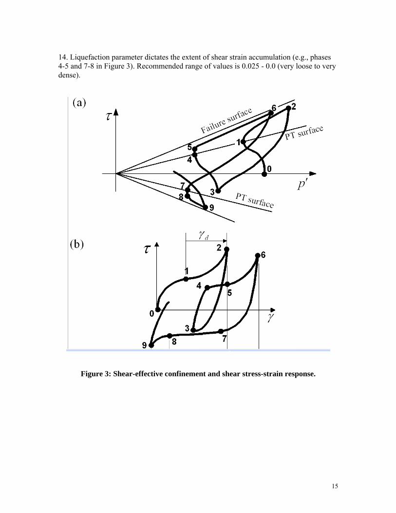
10. Number of yield surfaces (NYS). Suggested value is between 0 and 30 (Figure 2). In particular, NYS=0 dictates an elastic material (Parameters 7-9 are ignored, see Figure 2), NYS=1 indicates an elastic-perfectly plastic material (parameter 9 is ignored, see Figure 2). 11. Dilation angle in degrees. Dilation angle (Elgamal et al. 2003) divides the domain of shear-induced volume contraction response from that of volume dilation (via a Phase Transformation PT surface, see Figure 3). To remove contraction behavior completely, set this angle to zero. To remove dilation behavior completely, set this angle larger than the friction angle. 12. Below the Phase transformation PT surface (Figure 3): a) Contraction parameter 1 (c1) dictates the rate of pore pressure buildup under undrained conditions. Recommended range of values is 0.3 – 0.0 (very loose to very dense), and b) Contraction parameter 2 (c2) reflects the effect of overburden pressure on contraction behavior. Recommended range of values is 0.2 - 0.6 (very loose to very dense). As such, the level of excess pore-pressure buildup (or the decrease in effective confinement due to this contractive response, e.g., phase 0-1 in Figure 3) is dictated by a simple relationship of the form (Elgamal et al. 2003):

21 )(

cp

p c

a

where pa is atmospheric pressure.

13. Above the PT surface (Figure 3): a) Dilation parameter 1 (d1) dictates the rate of volume expansion (or reduction of pore pressure). Recommended range of values is 0.0 - 0.6 (very loose to very dense), and b) Dilation parameter 2 (d2) reflects the effect of accumulated shear strain on dilation behavior. Recommended value is 10. As such, the degree of regain in shear stiffness above the PT surface (due to this dilative response, e.g., phase 1-2 in Figure 3) is dictated by a simple relationship of the form (Elgamal et al. 2003):

)exp( 21 d d d .

15

14. Liquefaction parameter dictates the extent of shear strain accumulation (e.g., phases 4-5 and 7-8 in Figure 3). Recommended range of values is 0.025 - 0.0 (very loose to very dense).

Figure 3: Shear-effective confinement and shear stress-strain response.

16

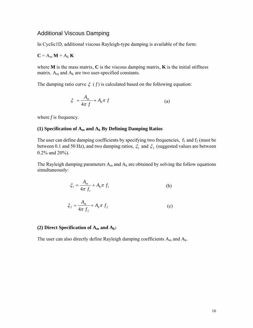
Additional Viscous Damping In Cyclic1D, additional viscous Rayleigh-type damping is available of the form: C = Am M + Ak K where M is the mass matrix, C is the viscous damping matrix, K is the initial stiffness matrix. Am and Ak are two user-specified constants. The damping ratio curve ( f ) is calculated based on the following equation:

fAf

Ak

m

4

(a)

where f is frequency. (1) Specification of Am and Ak By Defining Damping Ratios The user can define damping coefficients by specifying two frequencies, f1 and f2 (must be between 0.1 and 50 Hz), and two damping ratios, 1 and 2 (suggested values are between 0.2% and 20%). The Rayleigh damping parameters Am and Ak are obtained by solving the follow equations simultaneously:

11

1 4fA

f

Ak

m

(b)

22

2 4fA

f

Ak

m

(c)

(2) Direct Specification of Am and Ak: The user can also directly define Rayleigh damping coefficients Am and Ak.

17

Step-by-Step Time Integration Cyclic1D employs the Newmark time integration procedure with two user defined coefficients and (Newmark 1959, Chopra 2004). Standard approaches may be adopted by appropriate specification of these constants (Figure 4). Default values in Cyclic1D are 0.55, and ( ( + ½)2 ) / 4). Computations at any time step are executed to a convergence tolerance of 10-6 (Euclidean Norm of acceleration vector), normalized by the first iteration Error Norm (predictor multi-corrector approach). Users can modify the specified convergence tolerance. Note: An additional fluid-phase (Chan 1988) time integration parameter is set to 0.6 in the data file.

Figure 4: Newmark Time Integration

= 1/6 ; = 1/2 Linear acceleration (conditionally stable scheme) = 1/4 ; = 1/2 Average acceleration or trapezoidal rule (unconditionally stable

scheme in linear analyses); = 1/12 ; = 1/2 Fox-Goodwin (fourth order accurate)

18

Running the Analysis

To run the analysis, click “Save Model & Run Analysis” in Menu “Analyze” or “Save Model & Run Analysis” Button at the bottom of the Model Input window.

Upon the user requests to run the analysis, Cyclic1D will check all the entries defined by the user to make sure the model is valid. Thereafter, a small window will show the progress of the analysis.

By default, graphical output windows will be opened upon completion of the analysis.

To only verify if the input model is valid, choose “Check Input Data” in Menu “Analyze”.

Response at a Location

To view the response time histories, click “View Response Histories” in Menu “Output”.

The figures show the response histories at different depths (0m at ground surface and the largest at the bottom of the soil column).

Seven types of response time histories are available:

Horizontal Acceleration Time History

Response Spectrum of Acceleration (shown versus Period)

Response Spectrum of Acceleration (shown versus Frequency)

Fourier Transform Amplitude of Acceleration

Spectral amplification of acceleration relative to base motion

Horizontal Displacement Time History

Excess Pore Pressure Time History

Shear Stress versus. Shear Strain

Shear Stress versus. Effective Confinement

To zoom-in or zoom-out, use mouse to select a window. Click "fill" to get back to the original figure.

19

Response Profile

To view the response profiles, click “View Response Profile” in Menu “Output”. The figures show response profiles of the model. Seven types of response profiles are available:

Horizontal Displacement

Horizontal Acceleration

Excess Pore Pressure

Effective Confinement

Shear Strain

Shear Stress

To zoom-in or zoom-out, use mouse to select a window. Click "fill" to get back to the original figure.

20

Report Generator To get an analysis report in Microsoft Word Document format, click “Create a MS Word Report” in Menu “Report”. The report will include three sections: Model Input, Response Profile and Response History. Model Input If the check box “Include all model input parameters” is checked, the report will include all parameters of model input including model profile, input motion, soil properties and damping coefficients. If not, the user can select some of the above four types of model input parameters individually. Response Profile If the box “Include all response profile figures” is checked, the report will include all response profile figures including horizontal displacement, horizontal acceleration, excess pore pressure, effective confinement, shear strain and shear stress. If not, the user can select some of the above figures individually. Response at a Location By default, the check box “Include all figures of response at 0m depth (surface)” is checked. In this case, the report will include all seven types of response time histories at the surface (0m depth):

Horizontal Acceleration Time History

Response Spectrum of Acceleration

Fourier Transform Amplitude of Acceleration (versus Frequency)

Fourier Transform Amplitude of Acceleration (versus Period)

Spectral Amplification of Acceleration relative to base motion

Horizontal Displacement Time History

Excess Pore Pressure Time History

Shear Stress versus. Shear Strain

Shear Stress versus. Effective Confinement

21

If the above check box is unchecked, the user can select any response history figure at any depth (Figure 5).

LHS Box Depth Moving Buttons

RHS Box

Figure 5: Selector for Response History Figures in Report Generator

There are two list boxes (Figure 5): one (referred to as LHS box thereafter) is to list all of the depths that ARE NOT in the report,. The other (referred to as RHS box thereafter) is to list all of the depths that ARE in the report. The user can move a depth between the LHS box and the RHS box with one of the four buttons located between the two list boxes. Once the RHS box contains a depth or more, the user can select any figures (by checking or unchecking corresponding check boxes for a depth selected in the RHS box. The button “Check All” or “Uncheck All” right next to a response history figure can be used to facilitate a selection. Clicking a “Check All” button will include the response history figure right next to the button for ALL OF THE DEPTHS IN THE RHS BOX. Clicking a “Uncheck All” button will remove from the report the response history figure right next to the button for ALL OF THE DEPTHS IN THE RHS BOX. Note that a “Check All” button will become a “Uncheck All” button right after the user clicks it, or vice versa. File Location The report is in the form of a MS WORD file located in the working directory (see Installation for details).

22

Acknowledgments Cyclic1D is based on research underway since the early 1990s, and a partial list of related publications is included in the References section. The Cyclic1D graphical interface is written in Microsoft .NET Framework (Windows Forms). OxyPlot package (http://www.oxyplot.org) is employed for x-y plotting.

23

References Chan, A.H.C. (1988). "A Unified Finite Element Solution to Static and Dynamic Problems in Geomechanics," Ph.D. dissertation, U. College of Swansea, U. K. Chopra, A. “Dynamics of Structures (2000), “Theory and Applications to Earthquake Engineering”, Prentice Hall, Inc. Inglewood Cliffs, NJ Das, B.M. (1983). “Advanced Soil Mechanics,” Taylor and Francis Publisher. Das, B. M. (1995). Principles of Foundation Engineering, Third Ed., PWS Publishing Co., Boston, MA. Elgamal, A. -W. (1991). "Shear Hysteretic Elasto-Plastic Earthquake Response of Soil Systems,” Journal of Earthquake Engineering and Structural Dynamics, Vol. 20, No.4, 371-387, John Wiley Ltd. Elgamal, A., Yang, Z., Parra, E. and Ragheb, A. (2003). "Modeling of Cyclic Mobility in Saturated Cohesionless Soils,", Int. J. Plasticity, 19, (6), 883-905. Holtz, R.D. and Kovacs, W.D. (1981). An Introduction to Geotechnical Engineering, Prentice Hall, Englewood Cliffs, New Jersey. Hughes, T. (1987). “The Finite Element Method - Linear Static and Dynamic, Finite Element Analysis”, Prentice Hall, Inc., (1987). Kramer, S.L. (1996). Geotechnical Earthquake Engineering, Prentice Hall, Inc., Upper Saddle River, New Jersey, 653 pp. Newmark, N. M. (1959). “A Method of Computation for Structural Dynamics”, ASCE, Journal of the Engineering Mechanics Division, Vol. 85 No. EM3, (1959). Parra, E. (1996). “Numerical Modeling of Liquefaction and lateral Ground Deformation including Cyclic Mobility and Dilative Behavior is Soil Systems, PhD Dissertation, Department of Civil Engineering, Rensselaer polytechnic Institute, Try, NY. Prevost, J.-H. (1985). "A Simple Plasticity Theory for Frictional Cohesionless Soils," Soil Dynamics and Earthquake Engineering, 4(1), 9-17. Schnabel, P.B., Lysmer, J., and Seed, H.B. (1972). "SHAKE: A computer program for earthquake response analysis of horizontally layered sites," Report No. EERC 72-12, Earthquake Engineering Research Center, University of California, Berkeley, California. Seed, H.B. and Idriss, I.M. (1970). "Soil moduli and damping factors for dynamic response analyses," Report EERC 70-10, Earthquake Engineering Research Center, University of California, Berkeley.

24

Yang, Z. (2000). "Numerical Modeling of Earthquake Site Response Including Dilation and Liquefaction," Ph.D. Dissertation, Dept. of Civil Engineering and Engineering Mechanics, Columbia University, New York, NY. Zienkiewicz, O.C., Chan, A.H.C., Pastor, M., Paul, D.K. and Shiomi, T. (1990). "Static and Dynamic Behavior of Soils: A Rational Approach to Quantitative Solutions: I. Fully Saturated Problems," Proceedings, Royal Society of London, A 429, 285-309.

25

Appendix I: Cyclic1D-Related References

"Numerical Analysis of Seismically Induced Deformations In Saturated Granular Soil Strata," (1994), Ahmed M. Ragheb, PhD Thesis, Dept. of Civil Engineering, Rensselaer Polytechnic Institute, Troy, NY. "Identification and Modeling of Earthquake Ground Response," (1995), A. -W. Elgamal, M. Zeghal, and E. Parra, First International Conference on Earthquake Geotechnical Engineering, IS-TOKYO'95, Vol. 3, 1369-1406, Ishihara, K., Ed., Balkema, Tokyo, Japan, Nov. 14-16. (Invited Theme Lecture). "Prediction of Seismically-Induced Lateral Deformation During Soil Liquefaction," (1995), T. Abdoun and A. -W. Elgamal, Eleventh African Regional Conference on Soil Mechanics and Foundation Engineering, International Society for Soil Mechanics and Foundation Engineering, Cairo, Egypt, Dec. 11-15. "Liquefaction of Reclaimed Island in Kobe, Japan," (1996), A. -W. Elgamal, M. Zeghal, and E. Parra, Journal of Geotechnical Engineering, ASCE, Vol. 122, No. 1, 39-49, January. "Analyses and Modeling of Site Liquefaction Using Centrifuge Tests," (1996), E. Parra, K. Adalier, A. -W. Elgamal, M. Zeghal, and A. Ragheb, Eleventh World Conference on Earthquake Engineering, Acapulco, Mexico, June 23-28. "Numerical Modeling of Liquefaction and Lateral Ground Deformation Including Cyclic Mobility and Dilation Response in Soil Systems," (1996), Ender Parra, PhD Thesis, Dept. of Civil Engineering, Rensselaer Polytechnic Institute, Troy, NY. "Identification and Modeling of Earthquake Ground Response II: Site Liquefaction," (1996), M. Zeghal, A. -W. Elgamal, and E. Parra, Soil Dynamics and Earthquake Engineering, Vol. 15, 523-547, Elsevier Science Ltd. "Soil Dilation and Shear Deformations During Liquefaction," (1998a), A.-W. Elgamal, R. Dobry, E. Parra, and Z. Yang, , Proc. 4th Intl. Conf. on Case Histories in Geotechnical Engineering, S. Prakash, Ed., St. Louis, MO, March 8-15, pp1238-1259. "Liquefaction Constitutive Model," (1998b), A.-W. Elgamal, E. Parra, Z. Yang, R. Dobry and M. Zeghal, Proc. Intl. Workshop on The Physics and Mechanics of Soil Liquefaction, Lade, P., Ed., Sept. 10-11, Baltimore, MD, Balkema. "Modeling of Liquefaction-Induced Shear Deformations," (1999), A. Elgamal, Z. Yang, E. Parra and R. Dobry, Second International Conference on Earthquake Geotechnical Engineering, Lisbon, Portugal, 21-25 June, Balkema. "Numerical Modeling of Earthquake Site Response Including Dilation and Liquefaction," (2000), Zhaohui Yang, PhD Thesis, Dept. of Civil Engineering and Engineering Mechanics, Columbia University, NY, New York.

26

"Dynamic Soil Properties, Seismic Downhole Arrays and Applications in Practice," (2001), A.-W. Elgamal, T. Lai, Z. Yang and L. He, 4th International Conference on Recent Advances in Geotechnical Earthquake Engineering and Soil Dynamics, S. Prakash, Ed., San Diego, California, USA, March 26-31. "Computational Modeling of Cyclic Mobility and Post-Liquefaction Site Response," (2002), A. Elgamal, Z. Yang and E. Parra, Soil Dynamics and Earthquake Engineering, 22(4), 259-271. "Influence of Permeability on Liquefaction-Induced Shear Deformation," (2002), Z. Yang and A. Elgamal, J. Engineering Mechanics, ASCE, 128(7), 720-729. "Numerical Analysis of Embankment Foundation Liquefaction Countermeasures," (2002), A. Elgamal, E. Parra, Z. Yang, and K. Adalier, J. Earthquake Engineering, 6(4), 447-471. "Modeling of Cyclic Mobility in Saturated Cohesionless Soils," (2003), A. Elgamal, Z. Yang, E. Parra and A. Ragheb, Int. J. Plasticity, 19, (6), 883-905. "Application of unconstrained optimization and sensitivity analysis to calibration of a soil constitutive model ," (2003), Z. Yang and A. Elgamal, Int. J for Numerical and Analytical Methods in Geomechanics, 27 (15), 1255-1316. "Computational Model for Cyclic Mobility and Associated Shear Deformation," (2003), Z. Yang, A. Elgamal and E. Parra, J. Geotechnical and Geoenvironmental Engineering, ASCE, 129(12), 1119-1127. "A Web-based Platform for Live Internet Computation of Seismic Ground Response," (2004), Z. Yang, J. Lu, and A. Elgamal, Advances in Engineering Software, 35, 249-259. "Earth Dams on Liquefiable Foundation: Numerical Prediction of Centrifuge Experiments," (2004), Z. Yang, A. Elgamal, K. Adalier, and M. Sharp, J. Engineering Mechanics, ASCE, 130(10), 1168-1176. "Dynamic Response of Saturated Dense Sand in Laminated Centrifuge Container," (2005), A. Elgamal, Z. Yang, T. Lai, B.L. Kutter, and D. Wilson, J. Geotechnical and Geoenvironmental Engineering, ASCE, 131(5), 598-609. "Modeling Soil Liquefaction Hazards for Performance-Based Earthquake Engineering," (2001), "S. Kramer, and A. Elgamal, Pacific Earthquake Engineering Research (PEER) Center Report No. 2001/13, Berkeley, CA.

27

Appendix II: Built-in Soil Materials in Cyclic1D: Parameters and Units

Notation and Symbols (please also see relevant manual sections about soil material models)  

Mass density (kg/m3) ρ Reference shear wave velocity (m/s) Vs ref Reference effective mean confinement (kPa) p’ ref Confinement dependence coeff. coeff Initial lateral/vertical confinement ratio K0 Cohesion (kPa) c Friction angle (degree) φ Peak shear strain (%) max Number of yield surfaces NYS Dilation or Phase Transformation (PT) angle (degree) PT angleContraction parameter 1 c1 Contraction parameter 2 c2 Dilation parameter 1 d1 Dilation parameter 2 d2 Liquefaction parameter 1 Liq Permeability coefficient (m/s) Perm k  Notes: 1. The 3 parameters below are not directly defined in the Cyclic1D user interface. Instead, the shear wave velocity Vs and the initial lateral/vertical confinement ratio K0 (K0 =ν /(1-ν) are defined. Vs equal to Sqrt(G/ ρ ) allows G to be calculated. From K0, ν is calculated and G and ν are used to calculate B. Shear modulus (kPa) G Bulk modulus (kPa) B Poisson's Ratio ν  

2. p’ is the effective mean confinement equal to ((v’ + h’ + h’)/ 3), where v’ is the vertical effective stress = ‘ x depth and ‘ is for dry soil and is taken automatically as ( ‘-water) for saturated soil. In the above, h is horizontal confinement K0 x v (or for saturated soil ’h is K0 x ’v).

3. Variation of shear modulus with confinement p’ is defined by: G = (Gref) (p’/(p’ref))^coeff (note that p’ = p for dry soil) For instance if coeff is 0.5, then G =( Gref) (p’/(p’ref)) ^0.5 and consequently Vs = (Vs ref )(p’/(p’ref)) ^0.25

28

Initial-stress-state Parameters

ρ G B ν Vs ref p’ ref coeff K0

Soil Type \ Unit kg/m3 kPa kPa m/s kPa

1. Loose Silt 1700 5.80E+04 1.80E+05 0.4 184.7 80 0.5 0.67

2. Loose Sand 1700 5.80E+04 1.80E+05 0.4 184.7 80 0.5 0.67

3. Loose Gravel 1700 5.80E+04 1.80E+05 0.4 184.7 80 0.5 0.67

4. Medium Silt 1900 7.85E+04 2.40E+05 0.4 203.3 80 0.5 0.67

5. Medium Sand 1900 7.85E+04 2.40E+05 0.4 203.3 80 0.5 0.67

6. Medium Gravel 1900 7.85E+04 2.40E+05 0.4 203.3 80 0.5 0.67

7. Med-Dense Silt 1999 1.00E+05 3.00E+05 0.4 223.7 80 0.5 0.67

8. Med-Dense Sand 1999 1.00E+05 3.00E+05 0.4 223.7 80 0.5 0.67

9. Med-Dense Gravel 1999 1.00E+05 3.00E+05 0.4 223.7 80 0.5 0.67

10. Dense Silt 2100 1.35E+05 4.00E+05 0.4 253.5 80 0.5 0.67

11. Dense Sand 2100 1.35E+05 4.00E+05 0.4 253.5 80 0.5 0.67

12. Dense Gravel 2100 1.35E+05 4.00E+05 0.4 253.5 80 0.5 0.67

13. Cohesive Soft 1300 1.30E+04 2.00E+05 0.4 100 50 0 0.67

14. Cohesive Med 1500 6.00E+04 3.00E+05 0.4 200 50 0 0.67

15. Cohesive Stiff 1800 1.62E+05 8.00E+05 0.4 300 50 0 0.67 

Stress-strain and Permeability Parameters (see relevant manual sections about soil models)

c φ max NYS PT angle c1 c2 d1 d2 Liq Perm k

Soil Type \ Unit kPa deg % deg m/s

1. Loose Silt 0.3 29 5 20 30 0.3 0.2 0 10 0.025 1.00E-07

2. Loose Sand 0.3 29 5 20 30 0.3 0.2 0 10 0.025 6.60E-05

3. Loose Gravel 0.3 29 5 20 30 0.3 0.2 0 10 0.025 1.00E-02

4. Medium Silt 0.3 31.4 5 20 26.5 0.19 0.2 0.2 10 0.015 1.00E-07

5. Medium Sand 0.3 31.4 5 20 26.5 0.19 0.2 0.2 10 0.015 6.60E-05

6. Medium Gravel 0.3 31.4 5 20 26.5 0.19 0.2 0.2 10 0.015 1.00E-02

7. Med-Dense Silt 0.3 35 5 20 24 0.06 0.5 0.4 10 0.01 1.00E-07

8. Med-Dense Sand 0.3 35 5 20 24 0.06 0.5 0.4 10 0.01 6.60E-05

9. Med-Den. Gravel 0.3 35 5 20 24 0.06 0.5 0.4 10 0.01 1.00E-02

10. Dense Silt 0.3 40 5 20 22 0.01 0.6 0.6 10 0.003 1.00E-07

11. Dense Sand 0.3 40 5 20 22 0.01 0.6 0.6 10 0.003 6.60E-05

12. Dense Gravel 0.3 40 5 20 22 0.01 0.6 0.6 10 0.003 1.00E-02

13. Cohesive Soft 18 5 20 1.00E-09

14. Cohesive Med. 37 5 20 1.00E-09

15. Cohesive Stiff 75 5 20 1.00E-09