selected applications of integer programming: a ... · acknowledgements this text has bene ted a...
TRANSCRIPT

Selected Applications of Integer Programming:
A Computational Study


Selected Applications of Integer Programming:A Computational Study
Geselecteerde toepassingen van geheeltallig programmeren:Een computationele studie
(met een samenvatting in het Nederlands)
Proefschrift
ter verkrijging van de graad vandoctor aan de Universiteit Utrecht
op gezag van de Rector Magnificus, Prof. Dr. H.O. Voorma,ingevolge het besluit van het College voor Promoties
in het openbaar te verdedigenop maandag 11 september 2000 des ochtends te 10.30 uur
door
Abraham Michiel Verweij
geboren op 29 oktober 1971te ’s-Gravenhage

promotor: Prof. Dr. J. van Leeuwen, Faculteit Wiskunde & Informaticaco-promotoren: Dr. Ir. K.I. Aardal, Faculteit Wiskunde & Informatica
Dr. G. Kant, Ortec Consultants bv, Gouda
ISBN 90-393-2452-2

Contents
Preface vii
Acknowledgements ix
1 Introduction 11.1 Problems and Goals . . . . . . . . . . . . . . . . . . . . . . . . . 11.2 Outline and Contribution . . . . . . . . . . . . . . . . . . . . . . 21.3 Computational Environment . . . . . . . . . . . . . . . . . . . . 31.4 Definitions and Notational Conventions . . . . . . . . . . . . . . 4
I Foundations 7
2 Branch-and-Bound and Linear Programming 92.1 Introduction . . . . . . . . . . . . . . . . . . . . . . . . . . . . . . 92.2 Optimisation Problems . . . . . . . . . . . . . . . . . . . . . . . . 92.3 Branch-and-Bound . . . . . . . . . . . . . . . . . . . . . . . . . . 112.4 Linear Programming . . . . . . . . . . . . . . . . . . . . . . . . . 15
3 LP-Based Branch-and-Bound 193.1 Introduction . . . . . . . . . . . . . . . . . . . . . . . . . . . . . . 193.2 An LP-Based Branch-and-Bound Algorithm . . . . . . . . . . . . 213.3 Branch-and-Cut . . . . . . . . . . . . . . . . . . . . . . . . . . . . 313.4 Branch-and-Price . . . . . . . . . . . . . . . . . . . . . . . . . . . 383.5 Branch-Price-and-Cut . . . . . . . . . . . . . . . . . . . . . . . . 46
4 Maximum Independent Set 494.1 Introduction . . . . . . . . . . . . . . . . . . . . . . . . . . . . . . 494.2 Heuristics for Maximum Independent Set . . . . . . . . . . . . . 524.3 A Branch-and-Cut Algorithm . . . . . . . . . . . . . . . . . . . . 574.4 Computational Results . . . . . . . . . . . . . . . . . . . . . . . . 68
v

vi CONTENTS
II Applications 75
5 Map Labelling 775.1 Introduction . . . . . . . . . . . . . . . . . . . . . . . . . . . . . . 775.2 A Branch-and-Cut Algorithm . . . . . . . . . . . . . . . . . . . . 795.3 Computational Results . . . . . . . . . . . . . . . . . . . . . . . . 86
6 The Merchant Subtour Problem 936.1 Introduction . . . . . . . . . . . . . . . . . . . . . . . . . . . . . . 936.2 A Tabu Search Heuristic . . . . . . . . . . . . . . . . . . . . . . . 1016.3 A Branch-Price-and-Cut Algorithm . . . . . . . . . . . . . . . . . 1056.4 Computational Results . . . . . . . . . . . . . . . . . . . . . . . . 114
7 The Van Gend & Loos Problem 1197.1 Introduction . . . . . . . . . . . . . . . . . . . . . . . . . . . . . . 1197.2 Heuristics for The VGL Problem . . . . . . . . . . . . . . . . . . 1257.3 A Branch-and-Price Algorithm . . . . . . . . . . . . . . . . . . . 1337.4 Computational Results . . . . . . . . . . . . . . . . . . . . . . . . 135
Bibliography 139
Index of Notation 149
Samenvatting 153
Curriculum Vitae 157

Preface
We consider solving instances of mathematical optimisation problems by com-puter. This involves making a mathematical model for the problem at hand,designing an algorithm that is based on this model, and implementing and test-ing the algorithm. Often this leads to new ideas concerning the model, or thealgorithms we chose to use, or both, and then we have to adjust our solutionsto the newly gained insights. Clearly, such a study cannot succeed without theavailibility of interesting mathematical optimisation problems.
I consider myself to be a lucky PhD student, because I never had to inventmy own problems. My PhD-topic fitted in the European ALCOM-IT project(ALCOM-IT stands for ALgorithms and COMplexity in Information Technol-ogy), which had as a main goal to develop algorithms for industrial applications.My co-promoter Goos Kant participated in this project on behalf of Ortec Con-sultants bv, Gouda, The Netherlands. He ensured that I always had someproblems on which people from Ortec were working as well.
The first problem Goos brought to my attention originated from an anony-mous European airplane manufacturer that has production and assembly sitesall over Europe. While developing algorithms for this problem I first learnedabout integer programming and branch-and-bound algorithms. Using instancesof this problem I solved my first real linear programs. Although I learned a lotwhile working on this problem, it is not treated in this thesis. It is described ina technical report [118].
The second problem Goos brought into my life was an “easy” problem. Goosused to say that instances of it could be specified by “just two matrices of inputdata”. We named this problem “The Van Gend & Loos Problem”, after thecompany where it emerged. Chapters 6 and 7 treat this problem in detail. Itturns out that there is more to it than the two matrices Goos was referringto, which described the distances and the demands between customers. Traveltimes between customers and a fleet of vehicles that are stationed at a subsetof the sites of the customers complete the description of the problem. We willshow that this problem is NP-hard, and that even finding a feasible solution toit is NP-hard. And we will fail miserably in our effort to find provably optimalsolutions. Having said this, we are able to compute satisfactory solutions toinstances that are roughly half the size of the one given by Goos using prettysophisticated algorithmic techniques.
After having studied this problem for a while I decided to write my own
vii

viii PREFACE
code for it from scratch (except for the LP solver, that is). I felt that I did nothave full freedom in algorithmic design when using the frameworks that wereavailable. Apart from this I always underestimate the amount of work that goesinto implementing algorithms, and overestimate my own coding abilities. Thiswas in April 1998. Looking back, there is one big advantage of having your owncode, namely, that you really know what goes on after you hit return on thekeyboard to set the computer to work (and work, and work). In some way italso increases the fun of inspecting the result of the algorithm.
In order to develop and test my own code I needed instances of a problemwith a relatively clean problem structure. At first I used the knapsack problemfor this purpose, but after some time I decided that I needed a problem witha graph structure, and started to use instances of a map labelling problem.Apart from being interesting problems in their own right, instances of this maplabelling problem were easily accessible to me as Steven van Dijk, one of myPhD colleagues in the Computer Science Department, was developing geneticalgorithms for solving them. A variant of the map labelling problem can bereformulated as an independent set problem. It were these derived independentset instances that I used for testing my code. Even the earlier versions of itwere able to solve moderately sized map labelling instances within reasonabletime. Chapter 5 treats our approach to the map labelling problem in detail. Atthat time, I did not know that independent set problems are notoriously hard tosolve to optimality. Fortunately, my co-promoter Karen Aardal did know this.
Developing my own code for integer programming also meant learning abouthow people have solved integer programming problems in the past, even at timesback to before I was born. For me, this truly gave meaning to the word “student”in “PhD-student”. I hope that this thesis is as interesting for you to read asit was for me to learn, develop, code, and test all the algorithms that form itscontents.
Utrecht, May 2000
Bram Verweij

Acknowledgements
This text has benefited a lot from comments and remarks by Karen Aardaland Jan van Leeuwen on the first draft. Comments by Erik Balder, Stan vanHoesel, Goos Kant, Alexander Martin and Laurence Wolsey further improvedthe quality of the text.
I thank Karen, first for being an excellent supervisor, and second for sendingme to conferences and workshops all over the world during my time as a PhD-student. These conferences and workshops turned out to be very inspiring to me(especially the Aussois workshops), and have played a key role in my choice ofalgorithmic techniques. I thank Goos for providing me with interesting problemsto work on.
I am grateful to my colleagues of the Computer Science Department ofUtrecht University for making it such a pleasant place to work as a PhD-student.Special thanks go to Han, Job, Joao, Michiel, Paul, Robert-Paul, Tycho, Valerieand Jasper Aukes. Finally, I thank Marjan for all the love and support that shegave me during the past four years.
Just before my summer break in 1997 I was moved from a room on thefirst floor that I shared with my colleagues Robert-Paul and Joao to a roomon the third floor that was all for myself. Afterwards I was sad about havingleft the first floor, which I thought of as PhD-paradise. In this mood I made aromantic picture of a palm beach on some paradise island on the white board(that is, as far as my artistic capabilities allowed). When I came back from mysummer break, the picture was still there and I decided to leave it. My friendsspontaneously started to add features to it, and at some point in time I startedkidding that I would make it the cover of my thesis, which eventually I did.
The people who contributed to the cover are, as far as I can remember, KarenAardal, Abdu Basher, Robert-Paul Berretty, Valerie Boor, Babette de Fluiter,Joachim Gudmundsson, Michiel Hagedoorn, Mikael Hammer, Paul Harrenstein,Eveline Helsper, Lennart Herlaar, Stan van Hoesel, Goos Kant, Judith Keijsper,Elisabeth Lenstra, Jan Karel Lenstra, Stefano Leonardi, Han-Wen Nienhuys,Joana Passos, Hans Philippi, Joao Saraiva, Petra Schuurman, Danielle Sent, JobSmeltink, Tycho Strijk, Edwin Veenendaal, Jacques Verriet, Tjark Vredeveld,Marjan de Vries, Chantal Wentink and Wieger Wesselink.
ix


Chapter 1
Introduction
1.1 Problems and Goals
Consider the problem of putting city names on a map. Each name has to beadjacent to the city it belongs to, and no two names are allowed to overlap.The problem is to put as many names on the map as possible, subject to theseconditions. This problem is known as a map labelling problem.
Next, consider the problem of a merchant that drives around in a van andmakes money by buying commodities where they are cheap and selling them inother places where he can make a profit. Assuming that we know the prices forall of the commodities in all of the places and the cost of driving from one placeto another, the problem the merchant faces each day is to select a subset of thecities that he can visit in a day, and that maximises the profit he makes. Wecall this problem the merchant subtour problem.
Finally, consider a vehicle routing problem in which we have at our disposala fleet of trucks that are stationed at several depots, and in which we are givena set of customers with an integral demand for different commodities. Eachcommodity originates from one customer and is destined for another customer.Goods of each commodity may be split into integral amounts for transportation.Assuming that we know the cost of driving from one place to another, theproblem is to transport all demand using the available trucks, minimising thetotal cost of driving. As this problem models a problem that arises at the VanGend & Loos company in the Netherlands (and it is the only problem in thisthesis that does so) we call it the Van Gend & Loos problem.
The problems described above have in common that they can be describedas optimisation problems in integral variables subject to linear constraints, witha linear objective function (for details, see Part II). Problems of this kind areknown as integer linear programming problems. Specific integer linear program-ming problems have been studied by many authors in the past. For a numberof these problems algorithms have been reported that solve them successfully.
Our first goal is to develop algorithms for the specific problems named above.
1

2 CHAPTER 1. INTRODUCTION
This includes developing heuristics that only report feasible solutions, and opti-misation algorithms that solve them to optimality. Our second goal is to studythe behaviour of the algorithms we develop. This involves analysing the timecomplexity and the quality of the solutions. For the problems we consider it isnot clear how to develop algorithms that allow for both a satisfactory analysisof the time complexity and a satisfactory analysis of the quality of the solutions.Indeed, heuristic algorithms often have a nice worst-case time complexity butlack a good guaranteed bound on the solution quality, whereas optimisationalgorithms do produce a solution that is as good as is possible but they oftendo not have a nice worst-case bound on the time complexity, i.e., a bound thatguarantees termination within reasonable time. Therefore, in order to measurethe behaviour of our algorithms from a perspective different from the worst-casewe study them by means of computational experiments.
When designing algorithms for the problems mentioned above we try totake advantage of similar studies of other specific integer linear programmingproblems that were successful and can be found in the literature. This is ourmain motivation to study branch-and-cut and branch-and-price algorithms, aswell as LP rounding , local search, and tabu search.
1.2 Outline and Contribution
This thesis is organised as follows. In Part I we describe the core of our opti-misation algorithms. In Part II we apply the algorithms presented in Part I tothe specific problems of our interest.
Part I starts with Chapter 2 that discusses the generic branch-and-boundalgorithm that is used for finding provably optimal solutions, reviews relevantissues of computational complexity, and reviews some results from the theory oflinear programming that we rely on. In Chapter 3 we discuss how the branch-and-bound algorithm can be refined for integer linear programming problems,leading to branch-and-cut, branch-and-price, and branch-price-and-cut algo-rithms. In Chapter 4 we study the maximum independent set problem, a classicalproblem that can be formulated as an integer linear programming problem, anddiscuss branch-and-cut and LP rounding algorithms for it. We are interested inthe maximum independent set problem because it is possible to reformulate themap labelling problem into it.
We proceed in Part II with Chapter 5 where we present our algorithms for themap labelling problem. These algorithms are a refinement of the algorithms fromChapter 4 for the maximum independent set problem. In Chapter 6 we presenta tabu search heuristic and a branch-price-and-cut algorithm for the merchantsubtour problem. Finally, a branch-and-price algorithm, and a related branch-and-price based heuristic for the Van Gend & Loos problem are presented inChapter 7. The algorithms from Chapter 7 use the ones from Chapter 6 assubroutines.
The models and algorithms that are discussed in Part I are well-documentedin the literature. However, when implementing them one has to make numer-
1.3. COMPUTATIONAL ENVIRONMENT 3
ous choices concerning details. Sometimes this has resulted in original featuresof our code. In particular, we like to mention the scheme for re-computingvariable bounds in each node of the branch-and-bound algorithm after an im-proving primal solution has been found, treated in Section 3.2.2, the improvedreduced cost arguments for tightening variable bounds, treated in Section 3.2.3(these were developed together with Strijk [107]), the combined variable/GUBbranching scheme from Section 3.2.5, the minimum regret rounding heuristic formaximum independent sets, treated in Section 4.2.2, the scheme for identifyingan odd hole and using a path-decomposition for lifting odd hole inequalities,treated in Section 4.3.3. To the best of our knowledge, these ideas have notbeen reported on before.
Our contribution in Part II is the following. For the map labelling problem,we are the first to report on an optimisation algorithm that can solve instances ofthe map labelling problem with up to 950 cities on a standard map to optimalitywithin reasonable time. An earlier version of our algorithm for map labellingwas reported on in Verweij and Aardal [117]. The recursive technique for settingvariables from Section 5.2.3 is new. The merchant subtour problem and theVan Gend & Loos problem are original, and all models and algorithms for itpresented in Chapters 6–7 are of our own design.
A major part of the work behind this thesis has been spent on implement-ing and testing all the algorithms to obtain experimental data. This effort isaccumulated in the sections on computational results. We ask the reader to payspecial attention to all the tables and figures in this thesis that describe thebehaviour of the algorithms we present, as only those tables and figures giveinsight into the practical value of the algorithms to which they refer. Finally,we mention that we are the first to report on computational experiments usingthe separation algorithm for finding maximally violated mod-k cuts of Caprara,Fischetti, and Letchford discussed in Section 3.3.5. For this reason we will studythe yield of this particular separation algorithm with a bit more detail.
1.3 Computational Environment
As this is a computational study, some words about the system on which we per-formed our computations are in order. All our computations were executed onSun workstations, using C++ as a programming language (see Stroustrup [109]).Unless otherwise mentioned, the Sun workstation was a 360MHz Sun Enter-prise 2 with 512 megabyte main memory and eight gigabyte swap space runningUNIX as OS. We use the Gnu gcc compiler, version 2.95.2, with maximal com-piler optimisations (–O3).
Our implementation consists of approximately 24350 non-blank lines of C++code in total, spread over 94 modules. Chapters 2 and 3 involve approximately11300 non-blank lines of C++ code, also including elementary data structuressuch as linked lists, skip lists [96], heaps, and hash-tables. Chapters 4, 5, 6, and 7involve approximately 3300, 1600, 6450, and 1700 lines of code, respectively.
When implementing algorithms one has to be aware of the possibility that

4 CHAPTER 1. INTRODUCTION
there are bugs in the implementation. Indeed, during the development of ourimplementation plenty of time was spend on tracing and eliminating bugs. Un-fortunately, this does not give a guarantee that our implementation is fullybug-free.
We have included in our implementation numerous checks that verify inter-mediate results. As these checks verify the consistency of what we compute andare mainly inspired by common sense we will refer to them as sanity checks.Our sanity checks include, among other things, verifying feasibility of solutionsproduced by our algorithms, watching bound clashes (i.e., bounds that contra-dict with feasible solutions produced by heuristics) and verifying the violationof reported violated inequalities (see Section 3.3). Equally important is thatwe do not turn these sanity checks off to obtain a better performance in termsof absolute CPU time. We can afford this because the CPU time used by thesanity checks does not determine the order of magnitude of the total CPU time.For all the experiments reported on in this thesis, our algorithms terminatednormally and no abnormalities were reported by any of the sanity checks. Thisis the reason why we are confident about the correctness of our implementation.
1.4 Definitions and Notational Conventions
To describe our algorithms unambiguously we need some notation. We adoptnotational conventions that are generally accepted by the integer programmingand combinatorial optimisation community. People who are familiar with stan-dard textbooks such as the ones by Nemhauser and Wolsey [88] and Grotschel,Lovasz, and Schrijver [55] should recognise most of our notation.
Sets, Vectors. By N (Z,R) we denote the set of natural (integral, real) num-bers. The natural numbers include 0. If S is a set, then the collection of allsubsets of S is denoted by 2S. If E and S are sets, where E is finite, then SE
is the set of vectors with |E| components, where each component of a vectorx ∈ SE is indexed by an element of E, i.e., x = (xe)e∈E . For F ⊆ E the vectorχF ∈ SE , defined by χFe = 1 if e ∈ F and χFe = 0 if e ∈ E \ F , is called theincidence vector of F . For F ⊆ E and x ∈ SE , the vector xF ∈ SF is thevector with |F | components defined by xF = (xe)e∈F . We use x(F ) to denote∑e∈F xe. For x ∈ SE , the set supp(x) = {e ∈ E | xe 6= 0} is called the support
of x, and the set {e ∈ E | xe /∈ Z} is called the fractional support. The vectorsx+ and x−, defined by x+
e = xe if xe ≥ 0, x+e = 0 if xe < 0, x−e = −xe if
xe ≤ 0, and x−e = 0 if xe > 0, such that x = x+ − x−, are called the positivepart and the negative part of x, respectively. All vectors are column vectors,unless stated otherwise.
Matrices. If I, J , and S are sets, where I and J are finite, then SI×J is theset of |I| by |J | matrices, where each element of a matrix A ∈ SI×J is indexed byan element from I×J , i.e., A = (aij)i∈I,j∈J . Let A ∈ SI×J . For I ′ ⊆ I, J ′ ⊆ J ,AI′J ′ ∈ SI
′×J ′ denotes the |I ′|× |J ′| matrix defined by (aij)i∈I′,j∈J ′ . For j ∈ J ,

1.4. DEFINITIONS AND NOTATIONAL CONVENTIONS 5
Aj ∈ SI denotes the jth column of A, i.e., Aj = AI{j}. For i ∈ I, ai ∈ SJ
denotes the ith row of A written as a column vector, i.e., ai = (A{i}J)T . ForJ ′ ⊆ J , AJ ′ ∈ SI×J
′denotes the |I| by |J ′| matrix defined by AJ ′ = AIJ ′ . For
I ′ ⊆ I, aI′ ∈ SI′×J denotes the |I ′| by |J | matrix defined by aI′ = AI′J . If A is
invertible, the inverse of A is denoted by A−1.
Undirected Graphs, Walks. An (undirected) graph G = (V,E) consists ofa finite nonempty set V of nodes and a finite set E of edges. Each edge e ∈ Eis an unordered pair e = {u, v}, u and v are called the endpoints of e. For eachS ⊆ V , let δ(S) = {{u, v} | u ∈ S, v ∈ V \ S} be the set of edges that haveexactly one endpoint in S. For v ∈ V , we write δ(v) instead of δ({v}). Givena subset S ⊆ V of nodes, we use E(S) = {{u, v} ∈ E | u, v ∈ S} to denote theset of edges with both endpoints in S. The graph with node set S and edge setE(S) is called the induced graph of S and is denoted by G[S] = (S,E(S)).
A walk from v0 to vk in G is a finite sequence of nodes and edges W =v0, e1, v1, . . . , ek, vk (k ≥ 0) such that for i = 1, 2, . . . , k, ei = {vi−1, vi} ∈ E.Node v0 is the called the start of W and node vk is called the end of W . Thenodes on W are denoted by V (W ) = {v0, v1, . . . , vk}, and the edges on W aredenoted by E(W ) = {e1, e2, . . . , ek}. The nodes {v1, v2, . . . , vk−1} are called theinternal nodes of W .
Directed Graphs, Walks. A directed graph G = (V,A) consists of a finitenonempty set V of nodes and a finite set A of arcs. Each arc a ∈ A is anordered pair a = (u, v), u and v are the endpoints of a, u is called the tailof a, and v the head. If a = (u, v) ∈ A is an arc, we will denote the reversearc of a by a−1, i.e., a−1 = (v, u). A directed graph is said to be complete ifA = {(u, v) | u, v ∈ V, u 6= v}. For each S ⊆ V , denote by δ+(S) = {(u, v) |u ∈ S, v ∈ V \ S} (δ−(S) = {(v, u) | u ∈ S, v ∈ V \ S}) the set of arcsleaving (entering, respectively) S. For v ∈ V , we write δ+(v) (δ−(v)) insteadof δ+({v}) (δ−({v}), respectively). Given a subset S ⊆ V of nodes, we useA(S) = {(u, v) ∈ A | u, v ∈ S} to denote the set of arcs with both endpointsin S. The directed graph with node set S and arc set A(S) is again called theinduced graph of S and is denoted by G[S] = (S,A(S)).
A walk from v0 to vk in G is a finite sequence of nodes and arcs W =v0, a1, v1, . . . , ak, vk (k ≥ 0) such that for i = 1, 2, . . . , k, ai = (vi−1, vi). Nodev0 is the called the start of W and node vk is called the end of W . The nodeson W are denoted by V (W ) = {v0, v1, . . . , vk}. The arcs on W are denoted byA(W ) = {a1, a2, . . . , ak}. The nodes {v1, v2, . . . , vk−1} are called the internalnodes of W .
Paths, Cycles, Holes. Suppose we are given an undirected (directed) graphG = (V,E) (G = (V,A)). A path in G is a walk in G in which all nodes aredistinct. We will denote a path from node u to node v by u v. A cycle(directed cycle) in G is a walk in G with v0 = vk in which all internal nodes aredistinct and different from v0. A chord in a cycle (directed cycle) C is an edge

6 CHAPTER 1. INTRODUCTION
{u, v} ∈ E (arc (u, v) ∈ A) with u, v ∈ V (C), but {u, v} /∈ E(C) ((u, v) /∈ E(C),respectively). A hole in G is a cycle in G without chords.

Part I
Foundations
7


Chapter 2
Branch-and-Bound andLinear Programming
2.1 Introduction
A central goal of this thesis is to study the behaviour of linear programming (LP)based branch-and-bound algorithms applied to a number of specific optimisationproblems. Although the details of these problems will differ considerably fromeach other, they can all be formulated as integer linear programming problems(see also Section 1.1). Integer programming problems can be seen as instancesof optimisation problems. We will formalise what we mean by optimisationproblems in Section 2.2. When an optimisation problem satisfies some modestconditions then we can design a branch-and-bound algorithm for it, the subjectof Section 2.3. A branch-and-bound algorithm can be seen as a divide-and-conquer algorithm which reduces the original optimisation problem we want tosolve to a (possibly large) number of relaxations related to the original problem.In the case of linear integer programming problems these relaxations are linearprogramming problems. In Section 2.4 we review some selected topics fromlinear programming. This chapter gives the basis for Chapter 3, which combinesbranch-and-bound with linear programming to obtain an algorithm for integerlinear programming problems.
2.2 Optimisation Problems
Although the problems that we will study in this thesis are very concrete, we willpresent the branch-and-bound core of our algorithms in terms of more abstractoptimisation problems. Moreover, we will use the abstractions to relate ourconcrete problems to the theory of computational complexity. We start bydefining optimisation problems in a way that suits our purposes.
9

10 BRANCH-AND-BOUND AND LP
Definition 2.1. An optimisation problem is defined by a collection of probleminstances, and is either a minimisation problem or a maximisation problem.An instance of an optimisation problem is a pair (X, z), where X is the set offeasible solutions, and z : X → R is the objective function.
Given an instance (X, z) of a maximisation (minimisation) problem, theproblem is to find x∗ ∈ X such that z(x∗) ≥ z(x) (or z(x∗) ≤ z(x), respectively)for all x ∈ X.
Definition 2.2. An instance (X, z) of a maximisation (minimisation) problemis feasible if X 6= ∅, and infeasible otherwise. It is bounded if there exists anupper (lower) bound on the value of the objective function over the elements ofX that is attained by a feasible solution, and unbounded otherwise.
To illustrate the intuition behind these definitions, consider the shortest pathproblem as an example. An instance of the shortest path problem is a pair (P, z)where P is given implicitly as the set of all paths in a graph G = (V,E) thatconnect two nodes s, t ∈ V , and the objective function z : P → R is given byz(P ) = c(E(P )) for some cost vector c ∈ RE . The shortest path problem is,given (P, z), to find a path P ∈ P that minimises z(P ). Since shortest pathsare not necessarily unique, a given problem instance may have more than oneoptimal solution.
Definition 2.3. Let (X, z) be an instance of a maximisation (minimisation)problem P . A relaxation P of P is an associated maximisation (minimisation)problem, where each instance (X, z) of P is associated with an instance (X, z)of P that satisfies
(i) X ⊇ X, and
(ii) z(x) ≥ z(x) (or z(x) ≤ z(x), respectively) for all x ∈ X.
We assume that the reader has some intuitive feeling for what algorithmsare. Informally, an algorithm for a problem is a well-defined computationalprocedure that takes a problem instance as input and produces a solution asoutput.
The notion of optimisation problem that is defined above suffices to in-troduce branch-and-bound algorithms. We will not be able to prove that thebranch-and-bound algorithms that we propose are any good in terms of worst-case guarantees on the asymptotic behaviour of these algorithms. On the otherhand they do solve the problems for which they are designed. In order to moti-vate our choice of algorithms, we use concepts from the theory of computationalcomplexity. To link optimisation problems to the theory of computational com-plexity we need the following:
Definition 2.4. The decision variant of an optimisation problem is definedby a collection of problem instances. An instance to the decision variant of anoptimisation problem P is a triple (X, z, ξ), where (X, z) is an instance of P ,and ξ ∈ R a threshold value.

2.3. BRANCH-AND-BOUND 11
Given an instance (X, z, ξ) of the decision variant of a maximisation (min-imisation) problem, the problem is to decide whether there exists a solutionx ∈ X such that z(x) ≥ ξ (or z(x) ≤ ξ, respectively). In our shortest pathexample, the decision variant of the shortest path problem is, given an instance(P, z, ξ), to determine whether there exists a path P ∈ P such that z(P ) ≤ ξ.
Definitions 2.1–2.4 do not make any assumptions on the way a problem in-stance is specified. For optimisation problems of interest the set of feasiblesolutions is given implicitly, and instances are encoded using a reasonable en-coding. The size of a problem instance is the length of its encoding. In ourshortest path example a reasonable way to specify an instance is by giving a4-tuple (G, s, t, c), which has a size of Θ(|V |+ |E|).
Define P to be the class of problems for which polynomial time algorithmsdo exist, and NP to be the class of problems for which solutions can be writtendown and verified in polynomial time of the size of the input. Cook’s theorem(see, e.g. Papadimitriou [93]) proves the existence of so-called NP-completeproblems in NP . These problems have the remarkable property that any poly-nomial time algorithm for it implies the existence of polynomial time algorithmsfor all problems in NP , and thus that P = NP . So far no polynomial timealgorithm has ever been developed for an NP-complete problem. On the otherhand, nobody has been able to show that P 6= NP . As a further introductionto computational complexity theory is beyond the scope of this thesis, we referto Papadimitriou [93] for details. The relation between optimisation problemsand their decision variants is treated in detail by Bovet and Crescenzi [21].
The decision variants of the optimisation problems we consider are all NP-complete problems. Therefore we do not expect to be able to devise polynomialtime algorithms for them. Instead we will study algorithms that either reportfeasible but not provably optimal solutions, or do not exhibit nice asymptoticbehaviour. We even consider algorithms that neither report provably optimalsolutions nor exhibit nice asymptotic behaviour. However, we will compare thequality of the solutions obtained with bounds on it, and we will establish at whatsize of problem instances this unfavourable asymptotic behaviour prevents usfrom finding solutions. This is done by means of computational experiments.We slightly abuse the theory of computational complexity by applying it tooptimisation problems: we say that an optimisation problem is NP-hard if itsdecision variant is NP-complete.
2.3 Branch-and-Bound
Branch-and-bound algorithms started to appear in the literature around nine-teen sixty. A survey of early branch-and-bound algorithms was given by Lawlerand Wood [78]. Our description of the branch-and-bound algorithm is reminis-cent of the one by Geoffrion [51], who uses Lagrangian relaxations.
Suppose we have an optimisation problem P and a relaxation P of P . Sup-pose further that for each instance (X, z) of P the associated instance (X, z) ofP has the following properties:

12 BRANCH-AND-BOUND AND LP
branchAndBound(X, z) // (X, z) is the instance of P we want to solve{S := {X}; z∗ := −∞; i = 1;while S 6= ∅ {
extract Xi from S;solve (P i): zi = max{z(x) | x ∈ Xi};if (P i) is feasible and zi > z∗ {
let xi be the best available solution to (P i);if xi ∈ X and z(xi) > z∗ {
x∗ := xi; z∗ := z(xi);
remove from S all Xj1 , X
j2 with zj ≤ z∗;
}if zi > z∗ {
add Xi1, X
i2 to S and store zi together with Xi
1, Xi2;
}}i := i+ 1;
}if z∗ = −∞ { return infeasible; } else { return x∗; }
}
Algorithm 2.1: The Branch-and-Bound Algorithm for Problem P
(i) Branching: we can partition each set X ′ ⊆ X of feasible solutions to Pinto three disjoint sets X ′1, X
′2, and X ′ \(X ′1∪X ′2) such that for all feasible
solutions x ∈ X ∩ X ′ to P we have either x ∈ X ′1 or x ∈ X ′2.
(ii) Bounding: for each set X ′ ⊆ X of feasible solutions to P that can beobtained by branching we know how to solve the relaxation (X ′, z) of theproblem instance (X ∩ X ′, z).
Assume that P is a maximisation problem and that P is either bounded orinfeasible. Observe that
max{z(x) | x ∈ X ∩ X ′} ≤ max{z(x) | x ∈ X ′} (2.1)
for all X ′ ⊆ X. Hence, property (ii) gives a way to bound the value of anyfeasible solution to P in X ′.
The branch-and-bound algorithm for P is defined as follows. The algorithmmaintains a collection S of disjoint subsets from X, the best known feasiblesolution x∗ ∈ X, and its value z∗ = z(x∗), and works in iterations1 starting
1A short summary of our notation: X denotes a set of feasible solutions to the problemof interest, X denotes a set of feasible solutions to its relaxation, Xi indicates a restrictedset of feasible solutions to the problem of interest associated with iteration i, Xi denotes aset of feasible solutions to its relaxation, and the sets Xi
1 and Xi2 are obtained from Xi by
branching.

2.3. BRANCH-AND-BOUND 13
from iteration 1. Upon termination, if P is feasible then x∗ will be an optimalsolution to it. Initially, we take S = {X}, and set z∗ to −∞. In iteration i, weextract a set from S, which we denote by Xi, and solve the relaxation
zi = max{z(x) | x ∈ Xi}. (2.2)
Note that we can do this because of property (ii), and that zi is an upper boundon the value of any solution in X∩Xi by (2.1). If problem (2.2) is infeasible, or ifzi ≤ z∗, we have a proof that there do not exist feasible solutions x ∈ X∩Xi thathave a larger objective function value than the best known solution and proceedwith iteration i+1. Otherwise, let xi be an optimal solution to problem (2.2). Ifxi is a feasible solution to P and z(xi) > z∗ we set x∗ = xi and z∗ = z(xi), andwe remove from S all sets Xj
1 and Xj2 with zj ≤ z∗. If zi > z∗ we use property
(i) to obtain disjoint sets Xi1, X
i2 that together contain all feasible solutions to
P in X ∩ Xi and add them to S. Having done this we proceed with iterationi + 1. The algorithm terminates when S becomes empty. If upon terminationz∗ = −∞ then the instance (X, z) is infeasible. Otherwise the algorithm returnsx∗. Pseudo-code is given in Algorithm 2.1.
The correctness of the branch-and-bound algorithm is seen as follows. De-note the value of z∗ at the end of iteration i by z∗i , and the set S at the end ofiteration i by Si. At the end of each iteration of the algorithm, each solutionx ∈ X that has a larger objective function value than the value z∗i of the bestknown solution in iteration i is contained in some set X ′ ∈ Si, i.e.,
for all x ∈ X with z(x) > z∗i there exists X ′ ∈ Si such that x ∈ X ′. (2.3)
Since upon termination S is empty and z∗ = z(x∗) if z∗ > −∞, either theredoes not exist a feasible solution or the reported solution x∗ is optimal. Thebranch-and-bound algorithm terminates if for any sequence Xi1 ⊇ Xi2 ⊇ · · ·we have that Xik ⊆ X for some finite index k. If n is an upper bound on anysuch index k, then the maximum number of relaxations solved is bounded by2n−1.
From (2.3) it follows that if Si 6= ∅, then the value
max{zi | Xik ∈ Si} (2.4)
is an upper bound on the value of the optimal solution to P . This can beused to obtain a good upper bound if one terminates the algorithm before onecompleted the enumeration.
With every execution of a branch-and-bound algorithm we can associatea rooted tree T that we call the branch-and-bound tree. Consider any finiteexecution of the branch-and-bound algorithm and let the last iteration in thisexecution be iteration N . With any iteration i, we associate a node vi in T(i ∈ {1, . . . , N}); node v1 is the root of the tree. For each iteration j > 1, weadd the edge {vi, vj}, where vi is uniquely determined by Xj = Xi
k for somek ∈ {1, 2}. The branch-and-bound tree T = (V,E), rooted at v1, is defined by
V = {vi | i ∈ {1, . . . , N}}, and
E = {{vi, vj} | Xj = Xik, k ∈ {1, 2}, j ∈ {2, . . . , N}}.

14 BRANCH-AND-BOUND AND LP
There are two ingredients of the branch-and-bound algorithm that we leftunspecified, namely, how to choose the relaxation Xi ∈ S in iteration i > 1,which is called the enumeration scheme, and how to choose the relaxationsXi
1, Xi2 after solving Xi, which is called the branching scheme. Both schemes
can influence the size of the branch-and-bound tree, and hence the running timeof the branch-and-bound algorithm. Note that if we can guarantee for a certainproblem P that the branch-and-bound tree has a polynomial size and that eachiteration terminates in polynomial time, then the branch-and-bound algorithmis a polynomial time algorithm for P . Hence, a branch-and-bound algorithmfor an NP-hard problem in which the relaxations solved by the algorithm arein P is unlikely to have an enumeration scheme or a branching scheme thatyields a polynomial size branch-and-bound tree. This explains why branchingrules and enumeration schemes that are encountered in the literature all havea heuristic nature. Branching schemes are problem specific, so we postponethe discussion of them until we apply branch-and-bound to concrete problems.Although enumeration schemes can be problem specific as well, there are anumber of enumeration schemes that can be mentioned within the abstractbranch-and-bound framework, namely, the depth-first, breadth-first, and best-first enumeration schemes.
A depth-first enumeration scheme chooses the relaxations in such a way thatthe sequence of nodes (vi)Ni=1 is a depth-first traversal of T , where T is the as-sociated branch-and-bound tree. The advantage of the depth-first enumerationscheme is that it steers towards the leaves of T , thus creating an opportunityto improve z∗ (or, if we are unlucky, find many infeasible relaxations). Dur-ing a depth-first traversal |S| is bounded by the maximum depth attained byany node in T , which make depth-first traversals efficient in terms of memoryrequirement. Another advantage of the depth-first enumeration scheme is thatit can be implemented easily using a recursive algorithm. Such a recursive al-gorithm can take maximal advantage of similarities between the relaxations ofadjacent nodes in the tree in order to decrease the computation time needed foreach node. A disadvantage of the depth-first enumeration scheme is that thedepth-first traversal can enter “the wrong part of the tree”, that is, a subtreeof T in which the relaxations associated with the nodes of the subtree do notcontain the optimal solution, or even worse, do not contain feasible solutionsx ∈ X. The branch-and-bound algorithm will not find this out until it hascompleted the computation in the subtree.
The breadth-first enumeration scheme chooses the relaxations in such a waythat the sequence of nodes (vi)Ni=1 is a breadth-first traversal of T . It does nothave the disadvantage of the depth-first enumeration scheme that it can digressinto the wrong part of the branch-and-bound tree. It does have the disadvantagethat it can take quite a long time before it encounters feasible solutions x ∈ X.
The best-first enumeration scheme chooses the relaxation with the best upperbound, i.e., in iteration i > 1 it chooses Xi = arg maxXjk∈Si z
j . Observe thatat the end of iteration i, the value of maxXjk∈Si z
j is an upper bound on thevalue of any solution x ∈ X that is contained in some relaxation X ∈ Si,

2.4. LINEAR PROGRAMMING 15
including all optimal solutions to the problem at hand. The advantage of thebest-first enumeration scheme is that it never chooses to solve a relaxation thatdoes not contribute to proving the optimality of these optimal solutions. Onthe other hand, the best-first enumeration scheme has the same disadvantageas the breadth-first enumeration scheme, in that it can take quite long before itencounters feasible solutions x ∈ X. In our computational experiments we willuse the best-first enumeration scheme.
We end our discussion of branch-and-bound with two observations. The firstobservation is that it does not matter for the correctness of the algorithm inwhat way we obtain our best feasible solution x∗. Therefore, if we have someheuristic for P that gives us a feasible x ∈ X, we can use it to initialise x∗ andz∗. Moreover, if we have a heuristic for P that maps solutions x ∈ X to x′ ∈ X,and this heuristic is reasonably fast, then we can apply it to the solution xi ineach iteration i for which xi /∈ X, and possibly improve upon the value of z∗.The second observation is that we can turn the branch-and-bound algorithminto a heuristic by just stopping it after a fixed time or iteration limit. If, atthe time we stop the algorithm, we have some feasible solution x∗, we take thisas the result. Otherwise, our heuristic has failed to find a solution.
2.4 Linear Programming
Linear programming was developed by Dantzig [33] in 1947. Textbooks on linearprogramming have been written, among others, by Dantzig [34], Chvatal [28],Bazaraa, Jarvis, and Sherali [16], Vanderbei [116], and Dantzig and Thapa [35].In this section we follow the exposition of Dantzig and Thapa ([35, Section 3.4]).Recall that the rank of a matrix A is the number of linearly independent rows(or columns) of A. An m× n matrix A (with m ≤ n) is of full rank if the rankof A is m.
Definition 2.5. Given natural numbers m,n, vectors c ∈ Rn, b ∈ Rm, and amatrix A ∈ Rm×n, the linear programming problem is to determine
max cTx (2.5a)subject to Ax = b (2.5b)
x ≥ 0. (2.5c)
Our interest will be mainly in the following variant of the linear programmingproblem.
Definition 2.6. Given natural numbers m,n, vectors c ∈ Rn, l,u ∈ Rn, b ∈Rm, and a matrix A ∈ Rm×n, the linear programming problem with boundedvariables is to determine
max cTx (2.6a)subject to Ax = b (2.6b)
l ≤ x ≤ u. (2.6c)

16 BRANCH-AND-BOUND AND LP
The function z(x) = cTx is called the objective function. In the remainderof this section we restrict our attention to linear programming problems withbounded variables.
Definition 2.7. A vector x ∈ Rn is called a feasible solution to (2.6) if itsatisfies (2.6b)–(2.6c).
In the following, to simplify the discussion we assume that A is of full rank.
Definition 2.8. A basis of A is a set {Aj1 , Aj2 , . . . , Ajm} of linearly independentvectors.
We will slightly overload terminology by calling the set of column indices{j1, j2, . . . , jm} a basis if {Aj1 , Aj2 , . . . , Ajm} is a basis. Denote the set of columnindices by J = {1, . . . , n}. The basic variables corresponding to a basis B ⊆ Jare the variables {xj | j ∈ B}. If B ⊆ J is a basis of A, then AB is an invertiblematrix. Suppose we have a basis B ⊆ J .
Definition 2.9. The vector x ∈ Rn is a basic solution corresponding to thebasis B ⊆ J if we can partition J \B into two disjoint sets J1, J2 ⊆ J \B (withJ1 ∪ J2 = J \B) such that
xJ1 = lJ1 , (2.7a)xJ2 = uJ2 , and (2.7b)
xB = A−1B (b−AJ\BxJ\B). (2.7c)
So, in a basic solution the variables xJ1 are at their lower bound, the variablesxJ2 are at their upper bound, and the values of the basic variables are solvedfor.
Definition 2.10. Given a vector π ∈ Rm, the reduced cost with respect to πis defined as the vector cπ ∈ Rn that is given by cπ = c− (πTA)T .
A fundamental result from the theory of linear programming is that, givena basis B, we can rewrite the objective function in terms of non-basic variables:
Proposition 2.1. Let A ∈ Rm×n, b ∈ Rm, c ∈ Rn, and let B ⊆ J be a basis ofA. If x satisfies (2.6b), then
cTx = πT b+ (cπJ\B)TxJ\B,
where πT = cTBA−1B .
Proof. Assume that x satisfies (2.6b). It follows that x also satisfies (2.7c).Hence,
cTx = cTBxB + cTJ\BxJ\B
= cTB(A−1B (b−AJ\BxJ\B)) + cTJ\BxJ\B
= cTBA−1B b− cTBA
−1B AJ\BxJ\B + cTJ\BxJ\B
= πTb+ (cTJ\B − cTBA−1B AJ\B)xJ\B
= πTb+ (cπJ\B)TxJ\B .

2.4. LINEAR PROGRAMMING 17
Theorem 2.2. (Reduced Cost Optimality Conditions) Let x∗ ∈ Rn be afeasible solution to (2.6), B ⊆ J a basis of A, and let πT = cTBA
−1B . If (x∗,π)
satisfies
cπj < 0 implies x∗j = lj, and
cπj > 0 implies x∗j = uj,for all j ∈ J , (2.8)
then x∗ is an optimal solution to (2.6).
Proof. Assume that (x∗,π) satisfies (2.8), and let x be an arbitrarily chosenfeasible solution to (2.6). Let J1 = {j ∈ J | cπj < 0} and J2 = {j ∈ J | cπj > 0}.Note that cπB = 0, so J1, J2 ⊆ J \B. By (2.8) and feasibility of x we have thatx∗J1≤ xJ1 and x∗J2
≥ xJ2 . By applying Proposition 2.1, we find that
cTx∗ − cTx = (cπJ\B)Tx∗J\B − (cπJ\B)TxJ\B
= (cπJ\B)T (x∗J\B − xJ\B)
= (cπJ1)T (x∗J1
− xJ1) + (cπJ2)T (x∗J2
− xJ2)≥ 0,
where the inequality is due to condition (2.8). Hence, cTx∗ ≥ cTx. Because xwas chosen arbitrarily, x∗ is optimal.
We refer to the process of determining whether (2.6) is infeasible, unbounded,or has a solution (x∗,π) satisfying the reduced-cost optimality conditions assolving (2.6).
Consider the following linear programming problem related to (2.5):
min bTπ (2.9a)
subject to ATπ ≥ c (2.9b)π ≶ 0. (2.9c)
A fundamental theorem from the theory of linear programming is the following:
Theorem 2.3. (Strong Duality Theorem) If (2.5) is unbounded then (2.9)is infeasible. If (2.9) is unbounded then (2.5) is infeasible. If (2.5) and (2.9) areboth feasible then cTx∗ = bTπ∗, where x∗ and π∗ are optimal solutions to (2.5)and (2.9), respectively.
The problem (2.9) is called the dual problem of (2.5). For further details ofthe theory of linear programming (including LP duality) we refer to the booksmentioned at the beginning of this chapter.
The original method proposed by Dantzig for solving linear programmingproblems is called the simplex method. The simplex method assumes that ithas as input a basis B ⊆ J with a corresponding basic feasible solution, thatit uses as a starting point. A variant of the simplex method, called the dualsimplex method, assumes that it has as input a basis B ⊆ J for which the

18 BRANCH-AND-BOUND AND LP
vector π = (cTBA−1B )T is part of a feasible solution to a linear program that
is dual to (2.6) (see Vanderbei [116, Chapter 9]). Although no polynomialtime bound has been shown to hold for any version of the simplex method,the algorithm performs very well in practice. A basic feasible solution to anylinear programming problem can be found, if it exists, by solving a derivedlinear programming problem with an obvious starting basis, at the cost of someextra computation time. There are various codes available that implement thesimplex method. In our implementations we make use of the CPLEX 6.5 linearprogramming solver [62].
It was shown by Khachiyan [69] that linear programming problems can besolved in polynomial time using an algorithm called the ellipsoid method (seee.g. Grotschel, Lovasz, and Schrijver [55]). The importance of this algorithm isthat it proves that linear programming is in P.

Chapter 3
LP-BasedBranch-and-Bound
3.1 Introduction
We have seen in Section 2.3 how to design branch-and-bound algorithms foroptimisation problems. In this thesis our focus is not on optimisation problemsin general, but on specific problems that are the subject of Part II. Each problemdiscussed in Part II of this thesis can be formulated as a mixed integer linearprogramming problem. A mixed integer linear programming problem can bedefined as follows. Given a matrix A ∈ Zm×n, vectors c, l,u ∈ Zn and b ∈ Zm,and a subset of the column indices J ⊆ {1, . . . , n}, find
max z(x) = cTx (3.1a)subject to Ax = b, (3.1b)
l ≤ x ≤ u, (3.1c)xJ integer. (3.1d)
The special case with J = {1, . . . , n} is called a (pure) integer linear program-ming problem. If in an integer linear program all variables are allowed to takevalues zero or one only, then it is called a zero-one integer linear programmingproblem. Let
P = {x ∈ Rn | Ax = b, l ≤ x ≤ u},
and
X = P ∩ {x ∈ Rn | xJ integer}.
Problem (3.1) is equivalent to
max{z(x) | x ∈ X},
19

20 CHAPTER 3. LP-BASED BRANCH-AND-BOUND
which is an instance of an optimisation problem in the sense of Definition 2.1.The LP relaxation of problem 3.1 is obtained by removing the constraints (3.1d),which yields the problem
max{z(x) | x ∈ P}. (3.2)
In this chapter we will study branch-and-bound algorithms that take advantageof the fact that LP relaxations can be solved efficiently. In case the entireformulation can be stored in the main memory of the computer, one can applythe basic LP-based branch-and-bound algorithm. However, it may occur thatA is given implicitly, and in this case m and n can even be exponential in thesize of a reasonable encoding of the problem data. Sometimes we are still ableto handle such problems using some modification of the basic LP-based branch-and-bound algorithm. These modifications lead to so-called branch-and-cut,branch-and-price, and branch-price-and-cut algorithms, corresponding to thecases in which only a subset of the constraints, a subset of the variables, andboth a subset of the constraints and of the variables are kept in main memory,respectively.
The area of integer linear programming was pioneered by Gomory [53] whodeveloped his famous cutting plane algorithm for integer linear programmingproblems in the nineteen fifties. Two of the first branch-and-bound algorithmsfor integer linear programming were developed by Land and Doig [74] andDakin [32] in the early nineteen sixties. Since that time, many articles, booksand conferences have been devoted to the subject. Among the books on inte-ger programming we mention Papadimitriou and Steiglitz [94], Schrijver [104],Nemhauser and Wolsey [88], and Wolsey [125]. Recent surveys of branch-and-bound algorithms for integer programming are by Junger, Reinelt andThienel [67] and Johnson, Nemhauser, and Savelsbergh [66]. Together withthe papers by Padberg and Rinaldi [92] and Linderoth and Savelsbergh [79],these references are the main source of the ideas that led to the algorithmsin this chapter. Recently, approaches to integer linear programming that aredifferent from LP-based branch-and-bound have been reported on by Aardal,Weismantel and Wolsey [3].
The advances of the theory and the developments in computer hardware andsoftware during the past four decades have resulted in algorithms that are ableto solve relevant integer programming problems in practice to optimality. Thismakes linear integer programming an important subject to study.
Several software packages that allow for the implementation of customisedbranch-and-cut, branch-and-price, and branch-price-and-cut algorithms exist.Here we mention MINTO [84] and ABACUS [110]. In order to have full freedomof algorithmic design we have implemented our own framework for branch-and-cut, branch-and-price, and branch-price-and-cut, which we use in all computa-tional experiments that are reported on in this thesis. The goal of this chapteris to give the reader the opportunity to find out what we actually implemented,without having to make a guess based upon the literature we refer to.
The remainder of this chapter is organised as follows. We describe a basicLP-based branch-and-bound algorithm in Section 3.2. We describe our version

3.2. AN LP-BASED BRANCH-AND-BOUND ALGORITHM 21
of the branch-and-cut, branch-and-price, and branch-price-and-cut algorithmsin Sections 3.3, 3.4, and 3.5, respectively.
3.2 An LP-Based Branch-and-Bound Algorithm
Here we refine the branch-and-bound algorithm from Section 2.3 for linear in-teger programming. The relaxations solved in a node of the branch-and-boundtree are given in Section 3.2.1. Sometimes it is possible to improve the linearformulation of the problem in a part of the branch-and-bound tree by tighteningthe bounds on the variables. This is discussed in Sections 3.2.2 and 3.2.3. Weproceed by describing branching schemes that can be employed in Sections 3.2.4and 3.2.5.
3.2.1 LP Relaxations
Consider iteration i of the branch-and-bound algorithm. The LP relaxation wesolve in iteration i of the branch-and-bound algorithm is uniquely determinedby its lower and upper bounds on the variables, which we will denote by li andui, respectively. Let
P i = {x ∈ Rn | Ax = b, li ≤ x ≤ ui},and
Xi = {x ∈ P i | xJ integer}.The LP relaxation that we solve in iteration i, denoted by LPi, is given by
max{z(x) | x ∈ P i}, (3.3)
which is a linear program with bounded variables as discussed in Section 2.4.In the root node v1 we take l1 = l and u1 = u to obtain the LP relaxation (3.2)of the original problem (3.1).
Note that the matrix A is a constant. In an implementation of the LP-based branch-and-bound algorithm this can be exploited by maintaining onlyone LP formulation of the problem. When formulating LPi in iteration i of thebranch-and-bound algorithm, we do this by imposing the bounds li,ui in thisformulation.
Next, we keep track of the basis associated with the optimal solution to theLP relaxation that we solve in each node of the branch-and-bound tree. Howwe do this is explained in more detail in Section 3.2.2. Recall the constructionof the branch-and-bound tree from Section 2.3. Consider iteration i > 1 ofthe branch-and-bound algorithm. The optimal basis B ⊆ {1, . . . , n} associatedwith the parent of node vi in the branch-and-bound tree defines a dual solutionπ = (cTBA
−1B )T . Furthermore LPi is derived from the LP relaxation associated
with the parent of node vi in the branch-and-bound tree by modifying onlya small number of variable bounds. Therefore π is dual feasible to LPi, andwe can expect π to be close to optimal. This is exploited by solving the LPi
starting from π using the dual simplex algorithm.

22 CHAPTER 3. LP-BASED BRANCH-AND-BOUND
3.2.2 Tightening Variable Bounds and Setting Variables
Suppose we have at our disposal a vector x∗ ∈ X with z(x∗) = z∗. Consideriteration i of the branch-and-bound algorithm in which LPi was feasible, andsuppose we have solved it to optimality. Recall that our branch-and-boundalgorithm is correct as long as we do not discard any solution that is better thanour current best solution from the remaining search-space (or, more precisely,if we maintain condition (2.3) as invariant). We can exploit the informationobtained from the optimal solution of LPi to tighten the bounds li and ui. Theimproved bounds are based on the value z∗ and the reduced cost of non-basicvariables in an optimal LP solution.
Let (xLP,π) be an optimal primal-dual pair to LPi, where π = (cTBA−1B )T for
some basis B ⊆ {1, . . . , n}. Further, let zLP = z(xLP ), and let L,U ⊆ {1, . . . , n}be the sets of variable indices with cπL < 0 and cπU > 0. The reduced cost cπjcan be interpreted as the change of the objective function per unit change ofvariable xj . From the reduced cost optimality conditions (see Theorem 2.2) itfollows that xj = uj if cπj > 0 and xj = lj if cπj < 0. Using these observationsand the difference in objective function between the optimal LP solution andx∗ we can compute a new lower bound for xj if cπj > 0, and a new upper bound
for xj if cπj < 0. These improved bounds are given by li, ui ∈ Qn, where
lij =
max(lij , u
ij + d(z∗ − zLP)/cπj e), if j ∈ U ∩ J ,
max(lij , uij + (z∗ − zLP)/cπj ), if j ∈ U \ J ,
lij otherwise,
and
uij =
min(uij , l
ij + b(z∗ − zLP)/cπj c), if j ∈ L ∩ J ,
min(iij , lij + (z∗ − zLP)/cπj ), if j ∈ L \ J ,
uij , otherwise.
The following proposition proves the correctness of the improved bounds.
Proposition 3.1. All xIP ∈ Xi with z(xIP) ≥ z∗ satisfy li ≤ xIP ≤ ui.
Proof. Let xLP,π, zLP, L, U be as in the construction of z∗, i, li, ui. Assume
that there exists a vector xIP ∈ Xi with z(xIP) ≥ z∗. Since xIP ∈ Xi ⊆ P i wehave AxIP = b, so by Proposition 2.1 we can write
z(xIP) = πTb+ (cπL)TxIPL + (cπU )TxIP
U ,
and since xLP ∈ P i we can write
z(xLP) = πT b+ (cπL)TxLPL + (cπU )TxLP
U
= πT b+ (cπL)T liL + (cπU )TuiU .

3.2. AN LP-BASED BRANCH-AND-BOUND ALGORITHM 23
Observe that xIP ∈ Pi implies xIPL ≥ liL and xIP
U ≤ uiU , so xIPL − liL ≥ 0 and
xIPU −uiU ≤ 0. Now, choose j ∈ U arbitrarily. Note that xIP ∈ Xi ⊆ P i directly
gives xIPj ≥ lij . Moreover,
z∗ − zLP ≤ z(xIP)− z(xLP)
= (cπL)T (xIPL − liL) + (cπU )T (xIP
U − uiU )
≤ cπj (xIPj − uij).
Hence,
xIPj ≥ uij + (z∗ − zLP)/cπj .
If j ∈ U \ J this proves that xIPj ≥ lij . Otherwise, j ∈ U ∩ J , and xIP
j ≥ lij by
integrality of xIPj . Because j was chosen arbitrarily we have xIP ≥ li. The proof
that xIP ≤ ui is derived similarly starting from an arbitrarily chosen indexj ∈ L.
Denote the sub-tree of the branch-and-bound tree that is rooted at nodevi by Tvi . We can tighten the bounds on the variables after solving the LPin iteration i by replacing the bounds li,ui by l
i, ui. By Proposition 3.1 we
do not discard any solution satisfying the integrality conditions that is betterthan the current best solution x∗ in doing so, which means that we maintaincondition (2.3) as invariant. The improved bounds are used in all iterations ofthe branch-and-bound algorithm that are associated with a node in the branch-and-bound tree in the sub-tree rooted at node vi, the node in the branch-and-bound tree associated with iteration i. In our implementation of LP-basedbranch-and-bound we do not tighten the bounds on continuous variables.
When a variable index j ∈ {1, . . . , n} satisfies lij = uij we say that xj isset to lij = uij in iteration i (node vi). When a variable is set in the rootnode of the branch-and-bound tree, it is called fixed. If lij < uij , we say thatthat xj is free in iteration i (node vi). Variable setting based on reduced costbelongs to the folklore and is used by many authors to improve the formulationof zero-one integer programming problems (for example by Crowder, Johnson,and Padberg [31] and Padberg and Rinaldi [92]). The version in Proposition 3.1is similar to the one mentioned by Wolsey [125, Exercise 7.8.7].
Note that the new bounds are a function of π, zLP, and z∗. As a consequence,each time that we find a new primal solution in the branch-and-bound algorithmwe can re-compute the bounds. Suppose we find an improved primal solution initeration k. An original feature of our implementation of the branch-and-boundalgorithm is that we re-compute the bounds in all nodes vi of the branch-and-bound tree with i ∈ {1, . . . , k} that are on a path from the root node to a nodevk′ with k′ > k. In order to be able to do this, we store a tree T ′ that mirrorsthe branch-and-bound tree. Each node wi in T ′ corresponds to some iterationi of the branch-and-bound algorithm, and with wi we store its parent p(wi) inT ′, and the values of π, zLP, and z∗ for which we last computed the bounds

24 CHAPTER 3. LP-BASED BRANCH-AND-BOUND
in wi, and the bounds that we can actually improve in node wi. The values ofπ are stored implicitly by storing only the differences of the optimal LP basisbetween node wi and node p(wi).
The actual re-computation of bounds is done in a lazy fashion as follows. Initeration k of the branch-and-bound algorithm, we compute the path P from w1
to wk in T ′ using the parent pointers. Next, we traverse P from w1 to wk, andkeep track of the final basis in each node using the differences, and of the bestavailable bounds on each variable using the improved bounds that are storedin the nodes on P . Consider some node wi in this traversal. If the value of z∗
that is stored in wi is less than the actual value, we re-compute the bounds inwi. If any of the bounds stored in node wi contradicts with bounds stored in anode wj that preceded wi in the traversal, we have found a proof that Xk = ∅and we fathom node wk. If any of the bounds stored in node wi is implied bya bound stored in a node wj that preceded wi in the traversion, we remove itfrom node wi.
Consider an execution of the branch-and-bound algorithm and let η denotethe number of times we improve on the primal bound. For wi ∈ T ′ let J ′ denotethe non-basic variables in the final basis of node wi. Assuming that n � m,the time spent in the re-computation of bounds of node wi is dominated by there-computation of the reduced cost from the final basis of node wi, which is ofthe order
O(η|supp(AJ ′)|). (3.4)
In a typical execution of the branch-and-bound algorithm, we improve on thevalue of z∗ only a few times. Moreover, in our applications we use branch-and-cut and branch-and-price algorithms that call sophisticated and often time-consuming subroutines in each iteration of the branch-and-bound algorithm.These observations imply that the bound (3.4) is dominated by the runningtime of the other computations performed in iteration i of the branch-and-bound algorithm in our applications. We believe that the benefit of havingstrengthened formulations is worth the extra terms (3.4) in the running time ofthe branch-and-bound algorithm, as the improved formulations help in reducingthe size of the branch-and-bound tree.
3.2.3 GUB Constraints and Tightening Variable Bounds
Assume that row i of the constraints (3.1b) is of the form
x(Ji) = 1,
where the variables xJi are required to be non-negative and integer. In thiscase row i is called a generalised upper bound (GUB) constraint. A GUB con-straint models the situation in which we have to choose one option from a setof mutually exclusive options. GUB constraints were introduced by Beale andTomlin [17]. In any feasible integer solution exactly one j ∈ Ji has xj = 1.

3.2. AN LP-BASED BRANCH-AND-BOUND ALGORITHM 25
Whenever we have a formulation in which some of the constraints are GUBconstraints, we can exploit this by strengthening the bounds on those variablesthat are in a GUB constraint using a slightly stronger argument than the onepresented in Section 3.2.2 (see also Strijk, Verweij, and Aardal [107]). LetI ′ ⊆ {1, . . . ,m} be the set of row indices corresponding to GUB constraints.The conflict graph induced by the GUB constraints is the graph G = (V,E),where the node set V contains all variable indices that are involved in one ormore GUB constraints and the edge set E contains all pairs of variable indicesthat are involved in at least one common GUB constraint, i.e.,
V =⋃i∈I′ Ji, and
E = {{j, k} ⊆ V | j, k ∈ Ji, i ∈ I ′}.
For a variable index j ∈ V , we denote by N(j) the set of variable indices k thatare adjacent to j in G, i.e., N(j) = {k | {j, k} ∈ E}.
The stronger arguments can be applied to all variables that are involvedin at least one GUB constraint. For j ∈ V , whenever xj has value one, theGUB constraints imply that xN(j) = 0, and whenever xj has value zero theGUB constraints imply that for at least one k ∈ N(j) xk has value one. Thestrengthened argument for modifying the upper bound on xj takes into accountthe reduced cost of the variables xN(j), and the strengthened argument formodifying the lower bound on xj takes into account the reduced cost of thevariables xk and xN(k) for some properly chosen k ∈ N(j).
Let z∗ again denote the value of the best known solution in X. Consideriteration i in which (3.3) is feasible and let (xLP,π) be an optimal primal-dualpair to (3.3) in iteration i where π = (cTBA
−1B )T for some basis B ⊆ {1, . . . , n}.
Let zLP = z(xLP ), and let L,U ⊆ {1, . . . , n} be the maximal sets of variableindices with cπL < 0 and cπU > 0. The strengthened bounds l
i, ui ∈ {0, 1}V are
defined as
lij =
{max(0, 1 + d(z∗ − zLP)/min{−cπk | k ∈ N(j)}e), if j ∈ U ,0, otherwise,
and
uij =
{min(1, b(z∗ − zLP)/cπj c), if j ∈ L,1, otherwise,
where for each j ∈ V \ U
cπj = cπj − cπ(N(j) ∩ U).
Proposition 3.2. All xIP ∈ Xi with z(xIP) ≥ z∗ satisfy li ≤ xIP
V ≤ ui.
Proof. Let xLP,π, zLP, L, U be as in the construction of z∗, i, li, ui. Assume
that there exists a vector xIP ∈ Xi with z(xIP) ≥ z∗. As in Proposition 3.1 we

26 CHAPTER 3. LP-BASED BRANCH-AND-BOUND
can write
z(xIP) = πTb+ (cπL)TxIPL + (cπU )TxIP
U , and
z(xLP) = πTb+ (cπL)T liL + (cπU )TuiU .
Observe that xIP ∈ Pi implies xIPL ≥ 0 and xIP
U ≤ 1, so xIPU − 1 ≤ 0. Now,
choose j ∈ L∩V arbitrarily. Either xIPj = 0 or xIP
j = 1. In the case that xIPj = 0
we directly have xIPj ≤ uij since uij ≥ 0. So assume that xIP
j = 1. It follows thatxIPN(j) = 0. But then,
z∗ − zLP ≤ z(xIP)− z(xLP)
= (cπL)T (xIPL − liL) + (cπU )T (xIP
U − uiU )
≤ (cπL∩V )TxIPL∩V + (cπU∩V )T (xIP
U∩V − 1)
≤ cπj xIPj + (cπU∩N(j))
T (xIPU∩N(j) − 1)
= cπj − cπ(U ∩N(j)).
Since cπj − cπ(U ∩N(j)) < 0, we find
(z∗ − zLP)/(cπj − cπ(U ∩N(j))) ≥ 1.
Hence xIPj ≤ uij . Because j was chosen arbitrarily we have xIP
V ≤ ui.The proof that xIP
V ≥ li
is derived similarly starting from an arbitrarilychosen index j ∈ U ∩ V , assuming that xIP
j = 0, and using the observation thatxIPj = 0 implies xIP
k = 1 for some index k ∈ N(j), which in turn implies thatxIPN(k) = 0.
The strengthened criteria for setting variables based on reduced cost can betaken into account in an implementation that stores the reduced cost of thevariables in an array by replacing cπj by min{−cπk | k ∈ N(j)} for all j ∈ U andby cπj for all j ∈ L in this array. Having done this the strengthened bounds canbe computed as in Section 3.2.2. The extra time needed for pre-processing thearray is O(|E|).
3.2.4 Branching Schemes
Here we describe branching schemes for LP-based branch-and-bound. After wehave solved the LP relaxation (3.3) in iteration k, and we have found an optimalsolution xk ∈ P k but xk /∈ Xk, we have to replace P k by two sets P k1 and P k2 .
Branching on Variables
The most common branching scheme in LP-based branch-and-bound is to selectj ∈ J such that xkj is fractional and to define P k1 and P k2 as
P k1 = P k ∩ {x ∈ Rn | xj ≤ bxkj c}, and P k2 = P k ∩ {x ∈ Rn | xj ≥ dxkj e}.

3.2. AN LP-BASED BRANCH-AND-BOUND ALGORITHM 27
This scheme was first proposed by Dakin [32] and is called variable branching.Its correctness follows from the observation that every solution x ∈ X satisfiesxj ≤ bxkj c or xj ≥ dxkj e.
The choice of the index j can be made in different ways. One way is tomake a decision based on xk, possibly in combination with c and x∗. Anexample of such a scheme, which we will refer to as Padberg-Rinaldi branchingbecause of its strong resemblance with the branching rule proposed by Padbergand Rinaldi [92], is as follows. The goal here is to find an index j such thatthe fractional part of xkj is close to 1
2 and |cj | is large. For each j ∈ J , letfj = xkj − bxkj c be the fractional part of xkj . First, we determine the valuesL,U ∈ [0, 1] such that
L = maxj∈J{fj | fj ≤ 1
2}, and U = minj∈J{fj | fj ≥ 1
2}.
Next, given a parameter α ∈ [0, 1] we determine the set of variable indices
J ′ = {j ∈ J | (1− α)L ≤ fj ≤ U + α(1− U)}.
The set J ′ contains the variables that are sufficiently close to 12 to be taken into
account. From the set J ′, we choose an index j that maximises |cj | as the one todefine P k1 and P k2 as before. In our implementation we have α = 1
2 as suggestedby Padberg and Rinaldi.
Branching on GUB Constraints
Let xk ∈ P k be as above, and let J i = supp(ai) denote the support of row iof the constraint matrix. Suppose that row i is a GUB constraint and that xkJihas fractional components. Partition J i into two non-empty disjoint sets J i1, J i2.Observe that any x ∈ X satisfies x(J i1) = 0 or x(J i2) = 0. Hence, we can defineP k1 and P k2 by
P k1 = P k ∩ {x ∈ Rn | xJi1 ≤ 0}, and P k2 = P k ∩ {x ∈ Rn | xJi2 ≤ 0}.
The branching scheme defined this way is called GUB branching and is due toBeale and Tomlin [17]. GUB branching is generally believed to yield a morebalanced branch-and-bound tree of smaller height, and hence of smaller size.
Before we can apply GUB branching, we need a way to choose the sets J i1and J i2. The most common way to do this is by using an ordering of the variablesin J that is specified as input to the branch-and-bound algorithm. Then J ispartitioned in such a way that the elements of J i1 and J i2 appear consecutivelyin the specified order. If we have such an ordering then J is called a specialordered set (more details can be found in Nemhauser and Wolsey [88]).
We follow a different approach, which is motivated by the observation thatthe problems from Part II do not exhibit a special ordering. Our aim is tochoose J i1 and J i2 such that xk(J i1) and xk(J i2) are close to 1
2 . We do this byconsidering the problem
maxS{xk(S)|S ⊆ J,xk(S) ≤ 1
2}, (3.5)

28 CHAPTER 3. LP-BASED BRANCH-AND-BOUND
which is an instance of the subset-sum problem. A strongly polynomial timeapproximation scheme for the subset-sum problem was given by Ibarra andKim [61]. We use their algorithm to find J i1 such that (1 − 1
1000 )xk(S∗) ≤xk(J i1) ≤ 1
2 , where S∗ denotes an optimal solution to (3.5), and take J i2 = J \J i1.Note that the sets J i1, J i2 constructed this way will be non-empty if xkJ hasfractional components. The precision of 1
1000 in the calculation of J i1 is arbitrarybut seems to work well in our implementation.
3.2.5 Branching Decisions using Pseudo-Cost
Now that we have seen different branching schemes, we discuss how to choosebetween the options, that is, how to compare different branching decisions witheach other and how to decide on which one to apply. We do this by using degra-dation estimates, that is, estimates on the degradation of the objective functionthat are caused by enforcing the branching decision. Degradation estimateshave been studied by Driebeek [43], Tomlin [111], Benichou, Gauthier, Girodet,Hentges, Ribiere, and Vincent [18], Gauthier and Ribiere [49], and most recentlyby Linderoth and Savelsbergh [79].
Focus on iteration k of the branch-and-bound algorithm and let xk ∈ P k beas in Section 3.2.4. Observe that all branching decisions of Section 3.2.4 are ofthe form
P k1 = P k ∩D1, and P k2 = P k ∩D2,
where Db ⊆ Rn enforces the altered variable bounds for each b ∈ {1, 2}. Inthe following, we call Db a branch (b ∈ {1, 2}), and a pair (D1, D2) a branchingoption. Our goal is to decide which branching option to apply. Once we decidedto branch using a pair of branches (D1, D2) we will refer to it as a branchingdecision.
So we have a fractional xk, and after applying the ideas of Section 3.2.4 wefind ourselves with a set of branching options from which we have to choosethe one we will enforce. Denote the set of branching options by D, and letD = {(D1
1 , D12), . . . , (DN
1 , DN2 )}. Later in this section we will discuss in detail
how to obtain the set D. We may assume that xk /∈ Dib for all choices of (i, b).
For each D = Dib a measure of the distance from xk to D can be defined as
f(D) =
xkj − uj , if D = {x ∈ Rn | xj ≤ uj},lj − xkj , if D = {x ∈ Rn | xj ≥ lj},xk(J ′), if D = {x ∈ Rn | xJ ′ ≤ 0}.
Note that 0 < f(Dib) < 1 for all (i, b) ∈ {1, . . . , N} × {1, 2} if we select all
branching options as in Section 3.2.4. The per-unit degradation of the objectivefunction caused by enforcing Di
b is called the pseudo-cost of Dib, and is given by
pib =max{z(x) | x ∈ P k} −max{z(x) | x ∈ P k ∩Di
b}f(Di
b)
3.2. AN LP-BASED BRANCH-AND-BOUND ALGORITHM 29
for each (i, b) ∈ {1, . . . , N}× {1, 2}. Actually computing the pseudo-cost for allbranches is time consuming, and is not believed to result in improved runningtimes.
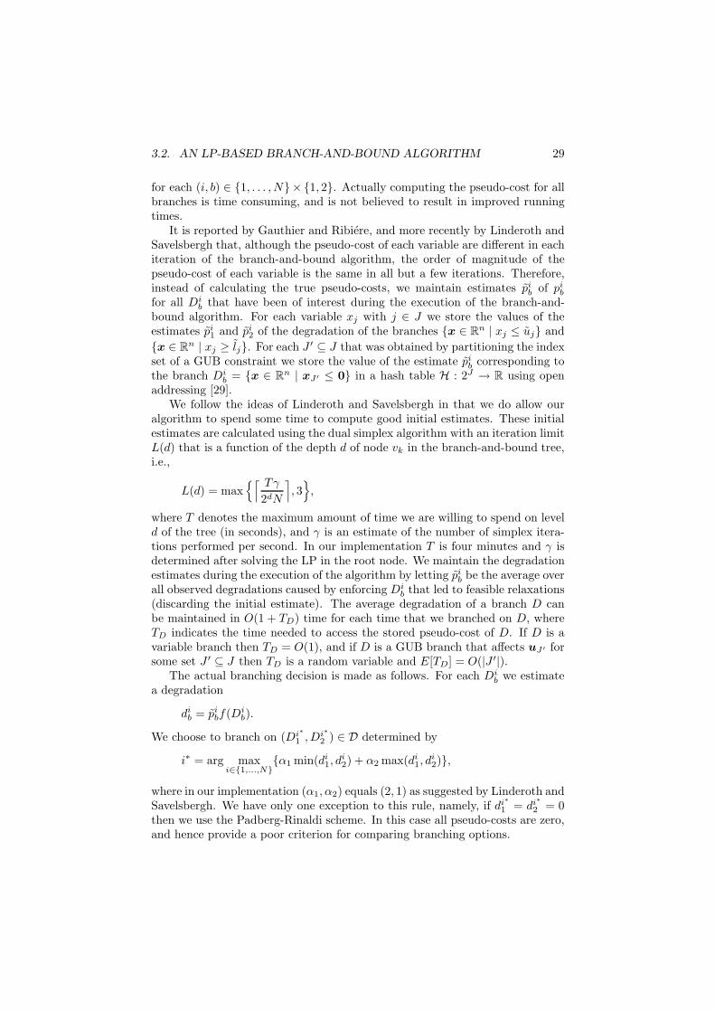
It is reported by Gauthier and Ribiere, and more recently by Linderoth andSavelsbergh that, although the pseudo-cost of each variable are different in eachiteration of the branch-and-bound algorithm, the order of magnitude of thepseudo-cost of each variable is the same in all but a few iterations. Therefore,instead of calculating the true pseudo-costs, we maintain estimates pib of pibfor all Di
b that have been of interest during the execution of the branch-and-bound algorithm. For each variable xj with j ∈ J we store the values of theestimates pi1 and pi2 of the degradation of the branches {x ∈ Rn | xj ≤ uj} and{x ∈ Rn | xj ≥ lj}. For each J ′ ⊆ J that was obtained by partitioning the indexset of a GUB constraint we store the value of the estimate pib corresponding tothe branch Di
b = {x ∈ Rn | xJ ′ ≤ 0} in a hash table H : 2J → R using openaddressing [29].
We follow the ideas of Linderoth and Savelsbergh in that we do allow ouralgorithm to spend some time to compute good initial estimates. These initialestimates are calculated using the dual simplex algorithm with an iteration limitL(d) that is a function of the depth d of node vk in the branch-and-bound tree,i.e.,
L(d) = max{⌈ Tγ
2dN
⌉, 3},
where T denotes the maximum amount of time we are willing to spend on leveld of the tree (in seconds), and γ is an estimate of the number of simplex itera-tions performed per second. In our implementation T is four minutes and γ isdetermined after solving the LP in the root node. We maintain the degradationestimates during the execution of the algorithm by letting pib be the average overall observed degradations caused by enforcing Di
b that led to feasible relaxations(discarding the initial estimate). The average degradation of a branch D canbe maintained in O(1 + TD) time for each time that we branched on D, whereTD indicates the time needed to access the stored pseudo-cost of D. If D is avariable branch then TD = O(1), and if D is a GUB branch that affects uJ ′ forsome set J ′ ⊆ J then TD is a random variable and E[TD] = O(|J ′|).
The actual branching decision is made as follows. For each Dib we estimate
a degradation
dib = pibf(Dib).
We choose to branch on (Di∗
1 , Di∗
2 ) ∈ D determined by
i∗ = arg maxi∈{1,...,N}
{α1 min(di1, di2) + α2 max(di1, d
i2)},
where in our implementation (α1, α2) equals (2, 1) as suggested by Linderoth andSavelsbergh. We have only one exception to this rule, namely, if di
∗
1 = di∗
2 = 0then we use the Padberg-Rinaldi scheme. In this case all pseudo-costs are zero,and hence provide a poor criterion for comparing branching options.

30 CHAPTER 3. LP-BASED BRANCH-AND-BOUND
To complete the description of our branching scheme, we have to specifyhow we obtain the set of branching options D. We do this by including in D allbranching options that are derived from fractional variables xj with j ∈ J . Inaddition, we add to D a selected number of branching options that are derivedfrom GUB constraints. One might be tempted to include in D a branchingoption derived from each GUB constraint that has fractional variables. However,if the number of GUB constraints in the formulation is relatively large then sucha scheme would waste too much time in selecting GUB constraints for branching,eliminating the potential benefit obtained from branch selection by pseudo-cost.
Instead we use the following approach, which takes into account that GUBconstraints may be added in later stages of the algorithm (this can occur in abranch-and-cut algorithm). Let I1 ⊆ {1, . . . ,m} denote the set of row-indicesof GUB constraints, so for each i ∈ I1 row i has the form
x(J i) = 1,
xJi ≥ 0, and J i ⊆ J . For each i ∈ I1 we keep track of the average pseudo-costpib of branches Di
b obtained by partitioning J i, that we use as a heuristic forecastof the pseudo-cost of the GUB branches obtained from row i in this iterationof the branch-and-bound algorithm (although the partitioning of J i, and hencethe resulting branching decision, might be totally different). We pre-select allGUB constraints that have at least four fractional variables in their support.Let I2 ⊆ I1 be the set of row indices corresponding to GUB constraints suchthat xJi has at least four fractional components for all i ∈ I2. Let I3 ⊆ I2 be theset of row indices corresponding to GUB constraints from which we did derivea branching option, and let I4 = I2 \ I3 be the set of row indices correspondingto GUB constraints from which we did not derive a branching option yet. Forthe rows indexed by I3 we already have a heuristic forecast of the pseudo-costof the branching decisions obtained from them, and for the rows indexed byI4 we have not. From I3, we select the K(d) constraints with highest averagepseudo-cost, and add those to I4. Here, K(d) is again a function of the depth dof node vk in the branch-and-bound tree, and is given by
K(d) = max{⌈ m
2d−1
⌉, 10}.
For each i ∈ I4 we partition J i as in the normal GUB branching procedure andadd the resulting pair of branches to D if the partition results in two sets J i1, J i2that each contain at least two fractional variables.
3.2.6 Logical Implications
Whenever we tighten variable bounds either by branching on them or by usingreduced cost criteria, we try to tighten more bounds by searching for logicalimplications of the improved bounds. This is done using the structure of theproblem at hand, so we do not go into detail here.
Consider iteration k of the branch-and-bound algorithm and let xk ∈ P k beas before. After enforcing the improved bounds obtained by calculating logical

3.3. BRANCH-AND-CUT 31
implications we obtain a relaxation
max{z(x) | x ∈ P k}
for some P k ⊂ P k. It may occur that xk /∈ P k. If this is the case then we iterateby resolving the strengthened LP, and proceed again with the strengthening ofvariable bounds.
3.3 Branch-and-Cut
In this section we refine the LP-based branch-and-bound algorithm from Sec-tion 3.2 in such a way that it is no longer necessary to include all constraintsin the LP formulation that is solved. The resulting refinement is known as abranch-and-cut algorithm, and allows us to use formulations with a large orpossibly exponential number of constraints. Formulations with an exponentialnumber of constraints are of interest because for some problems it is the onlyway to formulate them, and for other problems such formulations are signifi-cantly stronger than formulations of polynomial size. In both cases we need acutting plane algorithm to solve the linear program, explained in Section 3.3.1,that iteratively adds violated valid inequalities to the LP formulation. The cut-ting plane algorithm relies on problem-specific subroutines that are known asseparation algorithms. Some implementational issues that arise when dynami-cally adding constraints are discussed in Section 3.3.2. In Sections 3.3.3–3.3.5we review some known classes of valid inequalities together with their separationalgorithms, which we will use in Part II.
3.3.1 Valid Inequalities and The Cutting Plane Algorithm
Let P ⊆ Rn, and (π, π0) ∈ Rn × R. The inequality πTx ≤ π0 is valid for P if
P ⊆ {x ∈ Rn | πTx ≤ π0}.
Now, let P be a polyhedron in Rn and let πTx ≤ π0 be a valid inequality forP . The set
F = P ∩ {x ∈ Rn | πTx = π0}
is called a face of P . The valid inequality πTx ≤ π0 is said to define F . Wesay that F is a proper face of P if F 6= ∅ and F 6= P . A proper face is calleda facet if it is not contained in any other proper face of P . Facet-defining validinequalities are the strongest among all valid inequalities as they cannot beredundant (see e.g. Wolsey [125]). Recent surveys devoted to the subject ofvalid inequalities are by Aardal and van Hoesel [1] and by Marchand, Martin,Weismantel and Wolsey [82].
Recall the formulation of the mixed integer programming problem from Sec-tion 3.1. Let Π ⊆ Rn×R be such that each (π, π0) ∈ Π defines a valid inequalityfor conv(X). Then, the linear program
max{z(x) | x ∈ P , πTx ≤ π0 for all (π, π0) ∈ Π} (3.6)

32 CHAPTER 3. LP-BASED BRANCH-AND-BOUND
cuttingPlaneSolver(z, A, b, l,u, separation, α1, α2){
Π := ∅; i := 0;do { i := i+ 1;
solve LP max{z(x) | Ax = b, l ≤ x ≤ u,πTx ≤ π0 ∀(π, π0) ∈ Π};if LP infeasible return infeasible;let x∗ be an optimal solution of LP; zi := z(x∗);improve bounds and calculate logical implications, thus refining LP;if x∗ violates new bounds {
resolve LP;if LP infeasible return infeasible;let x∗ be an optimal solution; zi := z(x∗);
}Π′ := separation(x∗); Π := Π ∪ Π′;ξ := max(π,π0)∈Π′ π0 − πTx∗;
} while (i > 1 implies zi−1 − zi ≥ α1) and ξ ≥ α2 and Π′ 6= ∅;return x∗;
}
Algorithm 3.1: The Cutting Plane Algorithm
is a relaxation of the mixed integer programming problem (3.1). Hence, if wecan solve (3.6) efficiently, then we can incorporate it in an LP-based branch-and-bound algorithm.
The cutting plane algorithm to solve (3.6) works in iterations (starting from1), and maintains a set Π ⊆ Π. Initially, the set Π is empty. In iteration i, wesolve the linear program
max{z(x) | x ∈ P,πTx ≤ π0 for all (π, π0) ∈ Π}. (3.7)
If this problem is infeasible then the cutting plane algorithm reports so and ter-minates. Otherwise, let x∗ denote the optimal solution to (3.7), and let zi denotethe value of z(x∗). We first try to improve the bounds using Proposition 3.1. Ifthis succeeds we try to improve more bounds using logical implications as de-scribed in Section 3.2.6. If any of these implications are not satisfied by x∗, weresolve the LP. If the LP becomes infeasible, then we report so and terminate.Otherwise we update zi and x∗. The cutting plane algorithm then calls theseparation algorithm with x∗ as input, which returns a set Π′ ⊆ Π such thatfor each (π, π0) ∈ Π′ the valid inequality πTx ≤ π0 is violated by x∗. Let
ξ = max(π,π0)∈Π′
π0 − πTx∗
denote the maximum violation of any valid inequality defined by a pair (π, π0) ∈Π′. If Π′ is empty, or if i > 1, zi−1 − zi < α1 and ξ < α2, then the cuttingplane algorithm terminates and reports x∗ as solution. Otherwise, it adds Π′

3.3. BRANCH-AND-CUT 33
to Π and proceeds with the next iteration. The parameters (α1, α2) are used toavoid a phenomenon that is called tailing-off (see e.g. Padberg and Rinaldi [92]and Junger et al. [67]) of the cutting plane algorithm. Tailing-off occurs whenthe separation routines find cuts that do not add much to the strength of theformulation. If this is the case we are basically wasting precious CPU time. Inour implementation we have (α1, α2) = ( 1
100 ,110 ). Pseudo-code for the cutting
plane algorithm can be found in Algorithm 3.1.
3.3.2 Initialising LP Relaxations and Constraint Pools
When one uses a cutting plane algorithm to solve the LP relaxation in eachiteration, the question arises what constraints to keep in the LP formulationthat is maintained by the branch-and-bound algorithm. One possible answerwould be to keep all constraints that are generated by the separation routinesin the formulation. However, this would result in an LP formulation that keepsgrowing over the execution of the branch-and-cut algorithm. Therefore thelinear programs would take longer and longer to solve, which is undesirable..Keeping all constraints in the formulation is not what we will do.
Focus on any iteration i > 1, and let vj be the parent of node vi in thebranch-and-bound tree. Denote the optimal solution to LPj by xj . Padbergand Rinaldi [92] initialise the formulation in each iteration i > 1 with theconstraints of the matrix A, and the constraints generated by the separationroutines that were satisfied with equality by xj , This is the approach we fol-low. Note that all constraints with a non-basic slack variable are satisfied withequality. Initialising the LP formulation associated with iteration i is then ac-complished by eliminating valid inequalities from LPi−1 that are not satisfiedwith equality by xj , and adding those valid inequalities present in LPj that aresatisfied with equality and have a non-basic slack variable, next to imposing thebounds given in Section 3.2.1. The information about the status of the slackvariables of valid inequalities that are added to the LP formulation is handledin the same way as the information about optimal the basis in Section 3.2.2.
A second issue that arises when one uses the cutting plane algorithm andone initialises the LP formulations as above is the following. It might be ad-vantageous to cache constraints that are produced by the separation algorithmby storing them in a constraint pool, and then checking the constraint pool forviolated valid inequalities before calling the separation algorithm. Checking theconstraint pool for violated valid inequalities is called pool separation and is im-plemented by computing an inner product πTx for each valid inequality (π, π0)in the constraint pool and comparing the result with π0. If a constraint in thepool is violated in some iteration of the branch-and-cut algorithm, it is reportedas violated and not checked again for the remainder of this iteration. As sep-aration algorithms often solve non-trivial combinatorial optimisation problems,this can indeed be advantageous. However, the size of a constraint pool typi-cally grows over the execution of the algorithm, causing the pool separation totake longer and longer as the branch-and-cut algorithm proceeds.
Consider any iteration of the branch-and-cut algorithm and denote the set

34 CHAPTER 3. LP-BASED BRANCH-AND-BOUND
of valid inequalities in the constraint pool by
Π = {(πi)Tx ≤ πi0 | i ∈ {1, . . . , |Π|}}.
To avoid the pool separation from stalling our branch-and-cut algorithm, wedelete constraints from the constraint pool at certain times. For i ∈ {1, . . . , |Π|}we keep track of the number of iterations of the branch-and-bound algorithmki1 that the inequality (πi)Tx ≤ πi0 was in the pool since it was last inserted,and the number of iterations ki2 in which it was actually reported as violatedduring this period of time. The valid inequality (πi)Tx ≤ πi0 is kept in thepool at least as long as ki1 ≤ α1 for some parameter α1. However, as soon aski1 > α1 and ki2/k
i1 < α2 we delete it. The advantage of this scheme is that the
number of iterations that a constraint stays in the pool is linear in the number ofiterations in which it is actually reported as violated. In our implementation wehave (α1, α2) = (32, 1
5 ). In this way a constraint is kept for at least 32 iterationsand dropped as soon as it was not violated in at least 20% of the iterations thatit was in the pool, which appears to be a reasonable choice of parameters.
3.3.3 Cover Inequalities for Knapsack Sets
Suppose we are given a set of items N , a vector a ∈ NN that gives the size ofeach item in N , and a knapsack of size b ∈ N. Let
P = {x ∈ [0, 1]N | aTx ≤ b}.
The set
X = P ∩ {0, 1}N
contains all incidence vectors of subsets of N that fit in the knapsack and iscalled a knapsack set. Knapsack sets are of interest to us because they appearas a relaxation of the problem we discuss in Chapter 6. The set conv(X) isthe knapsack polytope, which has been studied since the mid-seventies by Pad-berg [90], Balas [8], Wolsey [122], Hammer, Johnson, and Peled [58], Crowder,Johnson and Padberg [31], and Weismantel [120]. Here we follow the expositionof Wolsey [125].
A cover is a set C ⊆ N such that a(C) > b. Let C be a cover. A coverinequality is an inequality of the form
x(C) ≤ |C| − 1, (3.8)
Cover inequalities are valid inequalities for the knapsack polytope. We say thatC is minimal if every proper subset C ′ ⊂ C has a(C ′) ≤ b. A minimal coverinequality is facet-defining if C = N .
A Greedy Heuristic for Searching Cover Inequalities
Suppose we are given a fractional solution x∗ ∈ P . To find a cover inequalitywe follow the approach presented by Crowder, Johnson and Padberg [31]. Let

3.3. BRANCH-AND-CUT 35
B ⊆ N be the fractional support of x∗, and let U ⊆ N \B be the maximal setof items with x∗U = 1. To separate a violated cover inequality, we focus on theset of items B with respect to a knapsack of size b′ = b− a(U). Note that thecover inequality (3.8) is equivalent to
|C| − x(C) ≥ 1.
Hence, there exists a cover C ⊆ B with respect to a knapsack of size b′ thatinduces a violated cover inequality in x∗ if and only if there exists a set C ⊆ Bwith a(C) > b′ that satisfies
|C| − x∗(C) < 1,
which is the case if
C∗ = arg minC⊆B
{∑i∈C(1− x∗i ) | a(C) > b′
}satisfies |C∗| − x∗(C∗) < 1.
The cover is computed using a greedy heuristic that first sorts the itemsin B in non-decreasing order of (1 − x∗i )/ai. Let B = {i1, . . . , i|B|} be theresulting ordering. The greedy algorithm proceeds with two stages. In the firststage it finds a cover, and in the second stage it turns it into a minimal cover.Finding a cover is done by determining the smallest index k such that the items{i1, . . . , ik} are a cover with respect to a knapsack of size b′, i.e., such thata({i1, . . . , ik}) > b′. Let k be this smallest index, and let C = {i1, . . . , ik}. Thesecond stage works in iterations, numbered j− 1, . . . , 1. In iteration l, we checkwhether C \ {il} has a(C \ {il}) > b′ and if so, we replace C by C \ {il}. Upontermination of the second stage the set C is a minimal cover, and the heuristicreturns it. The heuristic can be implemented in O(|B| log |B|) time.
The cover C that is returned by the heuristic need not be violated. Whetherit is violated or not, we will try to strengthen it using the lifting algorithm thatis the subject of the next section. If a cover inequality is violated after lifting,we report it.
3.3.4 Lifted Cover Inequalities for Knapsack Sets
Padberg [90], and Wolsey [122, 123] studied sequential lifting of valid inequal-ities. Sequential lifting of valid inequalities for zero-one integer programmingproblems relies on the following theorem (see also Nemhauser and Wolsey [88,Chapter II.2, Propositions 1.1 and 1.2]):
Theorem 3.3. Let S ⊆ {0, 1}n. For k ∈ {0, 1}, let Sk = S∩{x ∈ Rn | x1 = k}.
(i) Suppose
n∑j=2
πjxj ≤ π0 (3.9)

36 CHAPTER 3. LP-BASED BRANCH-AND-BOUND
is valid for S0. If S1 = ∅, then x1 ≤ 0 is valid for S. If S1 6= ∅, then
n∑j=1
πjxj ≤ π0 (3.10)
is valid for S for any π1 ≤ π0 −maxx∈S1{∑nj=2 πjxj}. If (3.9) defines a
face of conv(S0) of dimension k, and π1 is chosen maximal, then (3.10)defines a face of conv(S) of dimension k + 1.
(ii) Suppose that (3.9) is valid for S1. If S0 = ∅, then x1 ≥ 1 is valid for S.If S0 6= ∅, then
n∑j=1
πjxj ≤ π0 + π1 (3.11)
is valid for S for any π1 ≥ maxx∈S0{∑nj=2 πjxj} − π0. If (3.9) defines a
face of conv(S1) of dimension k, and π1 is chosen minimal, then (3.11)defines a face of conv(S) of dimension k + 1.
Theorem 3.3 is a special case of the theorem given by Wolsey [123, Theo-rem 1] for general integer programming problems.
Consider again the sets P and X defined by a set of items N , a vector a ∈ NNthat gives the size of each item, and a knapsack of size b as in Section 3.3.3.Suppose we are given a fractional solution x∗ ∈ P and that we have found acover inequality
x(C) ≤ |C| − 1 (3.12)
that is valid for the set{x ∈ {0, 1}N |
∑j∈C ajxj ≤ b− a(U)
},
using the separation algorithm described in Section 3.3.3, where U is again themaximal set of items such that x∗U = 1. Van Roy and Wolsey [113] give analgorithm that iteratively applies Theorem 3.3 starting from (3.12) to obtain alifted cover inequality of the form
x(C) +∑j∈D
αjxj ≤ |C| − 1 +∑j∈U
αj(1− xj),
where C,D and U are mutually disjoint sets of items. In each iteration, one coef-ficient αj is computed using a dynamic-programming algorithm for the knapsackproblem (see e.g. Nemhauser and Wolsey [88, Chapter II.6, Proposition 1.6]).Gu, Nemhauser and Savelsbergh [57] discuss modern implementations of thesetechniques.

3.3. BRANCH-AND-CUT 37
3.3.5 Mod-k Inequalities for Integer Programming
Suppose we are given natural numbers m,n, a matrix A ∈ Zm×n, and a vectorb ∈ Zm. Let
P = {x ∈ Rn | Ax ≤ b},
and let
X = P ∩ Zn.
A Chvatal-Gomory cut is a valid inequality for conv(X) of the form
λTAx ≤ bλT bc, (3.13)
where λ ∈ Rm+ satisfies λTA ∈ Zn. If λ ∈ {0, 1/k, . . . , (k − 1)/k}m for anyk ≥ 2, then the Chvatal-Gomory cut defined by λ is called a mod-k cut. Letλ ∈ {0, 1/k, . . . , (k − 1)/k}m. Given x∗ ∈ P , the violation achieved by x∗ ofthe mod-k cut defined by λ is given by
λTAx∗ − bλTbc.
Since λTAx ≤ λT b is satisfied by x∗, the maximal violation of a mod-k cutthat can be obtained by x∗ is (k − 1)/k. Mod-k cuts for which x∗ achievesthis violation are called maximally violated by x∗. The separation of mod-2cuts was studied by Caprara and Fischetti [22]. The separation of mod-k cutsas treated in this section is by Caprara, Fischetti, and Letchford [23, 24]. Thestudy of mod-k cuts is motivated by the fact that several well-known classes ofvalid inequalities for which no efficient separation algorithms were known, canbe interpreted as mod-k cuts. This includes the class of comb inequalities of thetravelling salesman problem.
Suppose we are given a fractional solution x∗ ∈ P . There exists a mod-kcut that is violated by x∗ if and only if there exists λ ∈ {0, 1/k, . . . , (k−1)/k}mwith
λTAx∗ − bλTbc > 0 and λTA ∈ Zn,
which is the case if and only if
ζ = maxλ{λTAx∗−bλT bc | λTA ∈ Zn,λ ∈ {0, 1/k, . . . , (k−1)/k}m
}(3.14)
satisfies ζ > 0. Let s∗ = b − Ax∗ denote the slack of x∗. By substitutingAx∗ = b − s∗, λT b − bλT bc = θ/k, and λ = 1
kµ in (3.14) and observing thatλTb− bλT bc = θ/k if and only if bTµ ≡ θ (mod k) and that λTA ∈ Zn if andonly if ATµ ≡ 0 (mod k), we obtain the equivalent formulation
ζ =1k
max(µ,θ) θ − (s∗)Tµ (3.15a)
subject to ATµ ≡ 0 (mod k), (3.15b)
bTµ ≡ θ (mod k), (3.15c)
(µ, θ) ∈ {0, . . . , k − 1}m+1. (3.15d)

38 CHAPTER 3. LP-BASED BRANCH-AND-BOUND
Caprara et al. show that (3.15) is NP-hard using a reduction from the max-imum cut problem. Furthermore, they show that the problem is polynomiallysolvable if we restrict ourselves to maximally violated mod-k inequalities. If(µ∗, θ∗) is an optimal solution to (3.15), then λ = 1
kµ∗ defines a mod-k cut
that is violated by x∗ if ζ > 0, and ζ is the violation obtained by x∗. LetI = {i ∈ {1, . . . ,m} | s∗i = 0} denote the set of row indices that have a slackequal to zero with respect to x∗. From the objective function of (3.15) it isimmediately clear that (µ∗, θ∗) defines a maximally violated mod-k cut if andonly if θ∗ = k − 1 and µ∗i = 0 for all i with s∗i > 0. From this it follows thata maximally violated mod-k exists if and only if the following system of mod-kcongruences has a solution:
ATI µ ≡ 0 (mod k), (3.16a)
bTI µ ≡ k − 1 (mod k), (3.16b)
µ ∈ {0, . . . , k − 1}I . (3.16c)
Determining feasibility of (3.16) and finding a solution to it if it is feasible can bedone in O(mnmin(m,n)) time if k is prime using standard Gaussian eliminationin GF (k). Moreover, they show that the existence of a maximally violated mod-k cut for any non-prime value of k implies the existence of a maximally violatedmod-l cut for every prime factor l of k. Therefore, we can restrict our attentionto the separation of maximally violated mod-k cuts for which k is prime.
In our implementation the system of mod-k congruences (3.16) is solvedby computing an LU -factorisation (see e.g. Chvatal [28]) of a sub-matrixof (3.16a)–(3.16b) that has full rank using arithmetic in GF (k) (see e.g. Cor-men et al. [29]), and checking the solution against the remaining constraints.To preserve the sparsity of the matrix we use a greedy heuristic that selects thenext pivot from the sparsest remaining non-zero row. Our implementation ispreliminary in that there are more sophisticated heuristics to preserve sparsity,and in that we compute the factorisation from scratch over and over again.
3.4 Branch-and-Price
Now that we have seen how to adapt the LP-based branch-and-bound algorithmfor integer linear programming formulations with a large number of constraints,we consider how to adapt the LP-based branch-and-bound algorithm in sucha way that it is no longer necessary to include all variables in the formulationthat is passed to the LP solver. This allows us to use formulations that have alarge, or even exponential number of variables. Problems that give rise to suchformulations have been studied since the nineteen eighties. These studies includethe ones by Desrosiers, Soumis, and Desrochers [40], Desrochers, Desrosiers,and Solomon [38], Barnhart, Johnson, Nemhauser, Savelsbergh, and Vance [14],Vanderbeck and Wolsey [115], and Vanderbeck [114].

3.4. BRANCH-AND-PRICE 39
3.4.1 LP Column Generation
Suppose we are given a matrix
A =(aI0aI\I0
)∈ Zm×n,
and a vector
b =(bI0bI\I0
)∈ Zm,
where m,n are natural numbers, and I0 ⊆ I = {1, . . . ,m} are sets of row indices.Consider the linear programming problem
max{z(x) = cTx | aI0x = bI0 ,x ∈ conv(X)}, (3.17)
where c ∈ Zn is the cost vector, and X is defined by the sub-matrix aI\I0 of Aand bound vectors l,u ∈ Zn as follows:
P = {x ∈ Rn | aI\I0x = bI\I0 , l ≤ x ≤ u}
and
X = P ∩ Zn.
We will reformulate (3.17) using Dantzig-Wolfe decomposition [36] to obtaina formulation with a possibly exponential number of variables. Suppose thataI\I0 has a block-diagonal structure, and let I1, . . . , Ik ⊆ I \ I0 and J1, . . . , Jk ⊆{1, . . . , n} be a partitioning of the row and variable indices of aI\I0 , respectively,such that
A =
A1 A2 . . . Ak
AI1J1
AI2J2
. . .AIkJk
, (3.18)
where Ai = AI0Ji . For each i ∈ {1, . . . , k}, let
Pi = {x ∈ RJi | AIiJix = bIi , lJi ≤ x ≤ uJi},
and
Xi = Pi ∩ ZJi .
To simplify the following discussion, assume that Xi is finite for each i ∈{1, . . . , k}.
Note that any fractional solution x ∈ conv(X) satisfies xJi ∈ conv(Xi), soxJi can be expressed as a convex combination of the elements of Xi:
xJi =∑x′∈Xi
x′λx′ , with λ(Xi) = 1, and λ ≥ 0.

40 CHAPTER 3. LP-BASED BRANCH-AND-BOUND
Now substituting for xJi in (3.17) yields an alternative linear programmingformulation to (3.17) with a large but finite number of λ-variables:
z∗(l,u) = maxk∑i=1
∑x∈Xi
(cTJix)λx (3.19a)
subject tok∑i=1
∑x∈Xi
(Aix)λx = bI0 , (3.19b)
λ(Xi) = 1, ∀i ∈ {1, . . . , k}, (3.19c)λ ≥ 0. (3.19d)
The linear programming problem (3.19) is referred to as the master problemthat we want to solve. The subscript (l,u) is added to the optimal value z∗ tostress the implicit dependence on the lower and upper bounds l and u.
Due to the large number of λ-variables it is difficult in general to solve (3.19)directly. Instead, we assume that we have at our disposal a relatively smallsubset Xi ⊆ Xi for each i ∈ {1, . . . , k}. In that case we can solve the followingrestricted master problem:
maxk∑i=1
∑x∈Xi
(cTJix)λx (3.20a)
subject tok∑i=1
∑x∈Xi
(Aix)λx = bI0 , (3.20b)
λ(Xi) = 1, ∀i ∈ {1, . . . , k}, (3.20c)λXi ≥ 0, ∀i ∈ {1, . . . , k}. (3.20d)
Suppose that the restricted master problem is feasible and that we have anoptimal primal-dual pair (λ, (π,µ)) to it, where π ∈ RI0 is associated withthe constraints (3.20b), and µ ∈ Rk is associated with the constraints (3.20c).Obviously λ is a feasible solution to the master problem, and (λ, (π,µ)) is anoptimal primal-dual pair to the master problem if it satisfies the reduced costoptimality conditions of Theorem 2.2. This is the case if for all i ∈ {1, . . . , k},for all x ∈ Xi, we have
cTJix− πTAix− µi ≤ 0,
which is the case if
ζi = max{(cπJi)Tx | x ∈ Xi} (3.21)
satisfies ζi ≤ µi, where cπ ∈ Rn is defined by cπJi = cJi − (πTAi)T for alli ∈ {1, . . . , k}. Problem (3.21) is called pricing problem i. If ζi > µi for somei ∈ {1, . . . , k}, then the corresponding optimal solution x∗ to pricing problemi is added to Xi, and the master problem is resolved. A column generation

3.4. BRANCH-AND-PRICE 41
algorithm iteratively solves a restricted master problem, and pricing problemsfor all i ∈ {1, . . . , k}, adding λ-variables that violate the reduced cost optimalityconditions of the master to the restricted master, until an optimal primal-dualpair to the master problem is found.
3.4.2 IP Column Generation
Now that we have seen how to apply Dantzig-Wolfe decomposition and columngeneration to linear programming problems, we will show how to adapt theLP-based branch-and-bound algorithm to integer linear programming problemsthat have a similar structure. For simplicity we concentrate on linear integerprogramming formulations that do not contain continuous variables. Considerthe integer linear programming problem
max{z(x) = cTx | aI0x = bI0 ,x ∈ X}, (3.22)
where b, c, A and I0 are as in the previous section, and X is again defined interms of aI\I0 , bI\I0 , l and u by
P = {x ∈ Rn | aI\I0x = bI\I0 , l ≤ x ≤ u}
and
X = P ∩ Zn.
Note that (3.17) is an LP relaxation of (3.22).Assuming that A is of the form (3.18) and after applying Dantzig-Wolfe
decomposition to (3.22) we obtain the following equivalent integer linear pro-gramming formulation with a large but finite number of λ-variables:
maxk∑i=1
∑x∈Xi
(cTJix)λx (3.23a)
subject tok∑i=1
∑x∈Xi
(Aix)λx = bI0 , (3.23b)
λ(Xi) = 1, ∀i ∈ {1, . . . , k}, (3.23c)
λXi ∈ {0, 1}Xi , ∀i ∈ {1, . . . , k}, (3.23d)
where Xi ⊆ ZJi , and Ai are defined as before. Problem (3.23) is called theIP master problem, and in the context of IP column generation its LP relax-ation (3.19) is called the LP master problem.
A branch-and-price algorithm for solving (3.22) is derived from the LP-basedbranch-and-bound algorithm as follows. The algorithm maintains a restrictedLP master problem, that we assume to be feasible. The situation that therestricted LP master problem is infeasible is discussed in Section 3.4.4. Asbefore, with each iteration j of the branch-and-price algorithm we associate a

42 CHAPTER 3. LP-BASED BRANCH-AND-BOUND
unique set of bounds lj ,uj ∈ Zn. In iteration j, the branch-and-price algorithmsolves the LP master problem obtained from (3.17) by imposing the boundslj ,uj instead of l,u. This is done by column generation. The formulation isobtained by imposing an upper bound of zero on all variables λx for whichljJi 6≤ xJi or xJi 6≤ u
jJi
, where xJi ∈ Xi, i ∈ {1, . . . , k}. The resulting pricingproblems are of the form
ζi = max{(cπJi)Tx | x ∈ Xi}, (3.24)
where for all i ∈ {1, . . . , k}
Xi = Pi ∩ ZJi ,
and
Pi = {x ∈ RJi | aIix = bIi , ljJi≤ x ≤ ujJi}.
If the pricing problems (3.24) are easy to solve, then we can use the columngeneration algorithm from Section 3.4.1 to solve the LP master problem in eachiteration of the branch-and-bound algorithm. However, it may very well be thatthe pricing problems (3.24) are NP-hard combinatorial optimisation problems.This is the case, for example, in Chapter 7 of this thesis, where we apply Dantzig-Wolfe decomposition to a vehicle routing problem, and the pricing problems arethe problems of how to route and load the individual vehicles. Under suchcircumstances it would be rather optimistic to believe that we can solve theLP master problems to optimality by column generation even for medium sizeproblems, as this would require us to solve numerous NP-hard pricing problemsin each iteration of the branch-and-price algorithm.
If we have an efficient heuristic for finding good feasible solutions to thepricing problems, we can use this heuristic to generate new columns insteadof spending a lot of time in optimising the pricing problems. However, thisapproach gives us a new problem, namely, that a restricted LP master problemitself is not a relaxation of the IP master problem (3.23). The value of therestricted LP master problem is only an upper bound for the value of the IPmaster problem if the optimal LP solution to the restricted LP master problemis also optimal to the LP master problem. This is not necessarily the case whenwe generate columns by solving the pricing problems using primal heuristics assuggested above.
A solution to this problem was observed by Vanderbeck and Wolsey [115],and was successfully applied by Vanderbeck [114]. Focus on iteration j ≥ 1 ofthe branch-and-price algorithm. Suppose we have solved a restricted master LPassociated with iteration j that was feasible, and let (π,µ) ∈ RI1×Rk be a dualsolution corresponding to an optimal basis B. Vanderbeck and Wolsey observethat if we have
ζi ≥ max{(cπJi)Tx | x ∈ Xi}, (3.25)

3.4. BRANCH-AND-PRICE 43
columnGenerationSolver(c′, A′, b′, l,u,pricing) // c′, A′ given implicitly,{ // returns λ∗, z ≥ z∗(l,u)
let X be a subset of the column indices of A′; // e.g. X := ∅;do { solve LP z := max{(c′X)TλX | A′XλX = b′,λX ≥ 0}
if LP infeasible {(X, feasible) := makeFeasible(A′, b′, l,u,X, pricing)if feasible {
solve LP z := max{(c′X)TλX | A′XλX = b′,λX ≥ 0}; }else { return infeasible; }
}let π be an optimal LP dual;(X ′, ζ, optimal) := pricing(π, l,u);
z := min(z, (b′)T (π + (0, ζ)T ));X := X ∪X ′;
} while X ′ 6= ∅ and ζ 6= 0;if optimal or ζ = 0 { z := z; }let λ∗X be an optimal LP solution;return (λ∗X , z);
}
Algorithm 3.2: Solving LP by Column Generation in Branch-and-Price
where Xi is defined as before for all i ∈ {1, . . . , k}, then the vector (π,µ+ ζ) is afeasible solution to the dual linear program of the LP master problem associatedwith iteration j. From this, by Theorem 2.3 it follows that
z∗(lj ,uj) ≤ bTπ + 1T (µ+ ζ),
and that λ∗ and (π,µ) are optimal solutions to the primal and dual LP masterproblem, respectively, if ζ = 0. Note that a value of ζ can be obtained by solvingrelaxations of the pricing problems, instead of the pricing problems themselves.
The IP master problem (3.23) can be restated as
max (c′)Tλ (3.26a)subject to A′λ = b, (3.26b)
λ ≥ 0, integer. (3.26c)
Pseudo-code of the LP column generation algorithm that we employ in ourbranch-and-price code is given in Algorithm 3.2. Note that A′ and c′ are givenimplicitly, i.e., in such a way that we can compute A′x and c′x for each x ∈⋃ki=1Xi once we have x. The pricing problems depend on the original problem
and are problem specific. Therefore, the column generation algorithm assumesas input a function pricing that it uses to solve the pricing problems. Thisfunction is of the form
pricing : Rm+k × Rn × Rn → 2⋃ki=1 Xi × Rk × {0, 1},

44 CHAPTER 3. LP-BASED BRANCH-AND-BOUND
and maps each triple (π, l,u) to a triple (X ′, ζ, f), where π is an optimal dualto the restricted LP master, l,u are bounds, X ′ is a set of column indicesthat correspond to λ variables that violated the reduced cost optimality criteriaof the LP master problem, ζ is an upper bound on the value of the pricingproblems, and f = 1 if the pricing problems were solved to optimality, and f = 0otherwise. Furthermore, the algorithm makes use of a function makeFeasible.Given a subset of the column indices X ′, bound vectors l,u, and the pricingfunction, makeFeasible determines whether there exists a set of column indicesX ′′ ⊇ X ′ such that A′X′′ = b′ is feasible. The function makeFeasible returns apair (X ′′, f), where f is 1 if A′X′′ = b′ and 0 otherwise.
3.4.3 The Branching Scheme
After we have solved the LP relaxation in some iteration i of the branch-and-price algorithm, we have at our disposal a vector λ∗ that is a feasible solutionto the LP master problem, and what we want to have is a feasible solution toour original problem (3.22). It is undesirable to branch on the λ-variables, asthis changes the structure of the pricing problems in all nodes that are not theroot node of the branch-and-bound tree. Indeed, we would have to prevent xfor which λx has been set to either zero or one to be regenerated by a pricingproblem. For the same reason we do not set λ-variables based on reduced costcriteria.
Several alternative branching schemes are reported in the literature. Here,we discuss a scheme that is known as branching on original variables (see e.g.Barnart et al. [14]). In this scheme, we compute x∗ ∈ Rn given by
x∗ =k∑i=1
∑x∈Xi
xλ∗x,
which is the same solution as λ∗ but restated in terms of the variables of theoriginal integer programming problem (3.22). If x∗ ∈ Zn, we are done. Oth-erwise we can select an index j∗ ∈ {1, . . . , n} such that x∗j∗ is fractional andpartition the feasible region by enforcing lower and upper bounds (li, ui) onone branch and (l
i,ui) on the other branch, where l
i, ui ∈ Zn are given by
lij =
{dx∗j e, if j = j∗,lij otherwise,
and uij =
{bx∗j c, if j = j∗,uij otherwise.
In our implementation the index j∗ is selected using the Padberg-Rinaldi rule(see Section 3.2.4).
We end this section by remarking that for the correctness of the branch-and-price algorithm it is necessary to branch if x∗ is integer but one does not havea proof that x∗ is optimal. This can be done in a similar way as above.
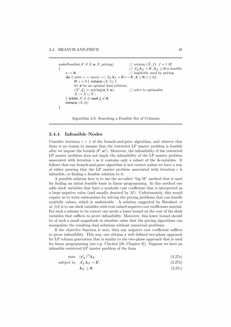
3.4. BRANCH-AND-PRICE 45
makeFeasible(A′, b′, l,u, X,pricing) // returns (X, f): f = 1 iff{ // A′
XλX = b′,λX ≥ 0 is feasible
c := 0; // implicitly used by pricingdo { solve z := max{−s | A′XλX + b′s = b′,λ ≥ 0, s ≥ 0};
if z = 0 { return (X, 1); }let π be an optimal dual solution;(X ′, ζ) := pricing(π, l,u); // solve to optimalityX := X ∪X ′;
} while X 6= ∅ and ζ 6= 0;return (X, 0);
}
Algorithm 3.3: Searching a Feasible Set of Columns
3.4.4 Infeasible Nodes
Consider iteration i > 1 of the branch-and-price algorithm, and observe thatthere is no reason to assume that the restricted LP master problem is feasibleafter we impose the bounds (li,ui). Moreover, the infeasibility of the restrictedLP master problem does not imply the infeasibility of the LP master problemassociated with iteration i as it contains only a subset of the λ-variables. Itfollows that our branch-and-price algorithm is not correct unless we have a wayof either proving that the LP master problem associated with iteration i isinfeasible, or finding a feasible solution to it.
A possible solution here is to use the so-called “big M” method that is usedfor finding an initial feasible basis in linear programming. In this method oneadds slack variables that have a symbolic cost coefficient that is interpreted asa large negative value (and usually denoted by M). Unfortunately, this wouldrequire us to write subroutines for solving the pricing problems that can handlesymbolic values, which is undesirable. A solution suggested by Barnhart etal. [14] is to use slack variables with real-valued negative cost coefficients instead.For such a scheme to be correct one needs a lower bound on the cost of the slackvariables that suffices to prove infeasibility. Moreover, this lower bound shouldbe of such a small magnitude in absolute value that the pricing algorithms canmanipulate the resulting dual solutions without numerical problems.
If the objective function is zero, then any negative cost coefficient sufficesto prove infeasibility. This way, one obtains a well defined two-phase approachfor LP column generation that is similar to the two-phase approach that is usedfor linear programming (see e.g. Chvatal [28, Chapter 8]). Suppose we have aninfeasible restricted LP master problem of the form
max (c′X)TλX (3.27a)subject to A′XλX = b′, (3.27b)
λX ≥ 0. (3.27c)

46 CHAPTER 3. LP-BASED BRANCH-AND-BOUND
To find a feasible solution to (3.27), we construct an auxiliary master linearprogram by replacing the cost vector c by the zero vector and adding a singleartificial variable s ∈ R with cost −1, and column b′:
max z(λ, s) = −s (3.28a)subject to A′λ+ b′s = b′, (3.28b)
λ ≥ 0, s ≥ 0. (3.28c)
Note that (λ, s) := (0, 1) is a feasible solution to (3.28) with value −1. Now,if λ∗ is a feasible solution to (3.27) then (λ∗, 0) is a feasible solution to (3.28)with value 0. Conversely, if (λ∗, s∗) is a feasible solution to (3.28) with value 0then s∗ = 0, so λ∗ is a feasible solution to (3.27). Pseudo-code for a procedurethat solves (3.28) by column generation to either prove infeasibility of the LPmaster problem, or to find a set of column indices X that defines a feasible LPmaster problem can be found in Algorithm 3.3. Note that in order to prove thatthe LP master problem associated with iteration i is infeasible, it is necessaryto solve the pricing problems to optimality.
3.5 Branch-Price-and-Cut
Consider again the integer linear programming problem
max{z(x) = cTx | aI0x = bI0 ,x ∈ X}, (3.29)
where b, c, A and I0 are as in the previous section, and X is again defined interms of aI\I0 , bI\I0 , l and u by
P = {x ∈ Rn | aI\I0x = bI\I0 , l ≤ x ≤ u}
and
X = P ∩ Zn.
Assume that A is of the form (3.18). We again apply Dantzig-Wolfe de-composition, but this time we leave xJ1 aside and only reformulate xJi fori ∈ {2, . . . , k}. In this way we obtain the following equivalent integer linearprogramming problem with a large but finite number of λ-variables:
max cTJ1xJ1 +
k∑i=2
∑x∈Xi
(cTJix)λx (3.30a)
subject to A1xJ1 +k∑i=2
∑x∈Xi
(Aix)λx = bI0 , (3.30b)
lJ1 ≤ xJ1 ≤ uJ1 , xJ1 integer, (3.30c)λ(Xi) = 1, ∀i ∈ {2, . . . , k}, (3.30d)
λXi ∈ {0, 1}Xi , ∀i ∈ {2, . . . , k}, (3.30e)

3.5. BRANCH-PRICE-AND-CUT 47
where Xi ⊆ ZJi , and Ai are defined as before. The resulting model can besolved using the branch-and-price algorithm of the previous section, allowingfor branching on the xJ1-variables as described in Section 3.2.4, and branchingon the original xJi-variables for i ∈ {2, . . . , k} as described in Section 3.4.3.
If we have one or more classes of valid inequalities for conv(X1) at our dis-posal, then we can add these to strengthen the LP formulation in each iterationof the branch-and-price algorithm. Furthermore, one may apply variable settingbased on reduced cost criteria to the xJ1 -variables whenever we have a proofthat the bound obtained from the restricted LP master problem is valid for theLP master problem. We will call the resulting algorithm a branch-price-and-cutalgorithm. A branch-price-and-cut algorithm applies a combined cutting planeand column generation algorithm to solve the LP relaxations in each iteration.In our implementation we alternate between rounds of column generation andseparation until the termination criteria of both the column generation algo-rithm and the cutting plane algorithm have been satisfied in two consecutiverounds.


Chapter 4
Maximum Independent Set
4.1 Introduction
Given an undirected graph G = (V,E), an independent set in G is a subsetS ⊆ V such that no two nodes in S are connected in G, i.e. for all edges{u, v} ∈ E we have that {u, v} 6⊆ S. The maximum independent set problem isthe problem of finding an independent set of maximum cardinality in a givengraph. Independent sets are sometimes called stable sets, vertex packings, ornode packings.
The complement of G has the same node set, and is denoted by G = (V, E)where {u, v} ∈ E if and only if {u, v} /∈ E. A clique in G is a set of nodes S ⊆ Vsuch that for all {u, v} ∈ S, {u, v} ∈ E. A subset S ⊆ V is an independentset in G if and only if S is a clique in G. The maximum clique problem is theproblem of finding a clique of maximum cardinality in a given graph. Due to theequivalence between independent sets in a graph and cliques in its complement,any algorithm for finding a maximum independent set also gives an algorithmfor finding a maximum clique, and vice versa.
Also, independent set problems are related to so-called set packing problems,in which one is given a ground set and a collection of subsets of this ground set,and one has to find a sub-collection of the given subsets that are disjoint andmaximal with respect to some objective function. The reduction from the setpacking problem to the independent set problem uses a conflict graph that issimilar in spirit as the one that is used in Section 3.2.3. For more details on setpacking and its relation to independent set problems we refer to Borndorfer [20]and Marchand, Martin, Weismantel, and Wolsey [82].
4.1.1 Motivation, Literature, and Chapter Outline
Several optimisation algorithms for finding maximum independent sets [101,106, 81, 80, 85, 126, 48] and maximum cliques [12, 6, 7, 26, 13] have been reportedon in the literature. Moreover, several real-life problems can be formulated asindependent set problems [100, 2, 117, 129]. The polyhedral structure of the
49

50 CHAPTER 4. MAXIMUM INDEPENDENT SET
independent set polytope has been reported on by various authors [90, 86, 87,112].
Our interest in independent set problems originates from the fact that maplabelling problems, which are the subject of Chapter 5, can be reformulatedas independent set problems. We develop a number of powerful techniquesfor the problem that are meant to work well on sparse large-size instances.We do not claim that our independent set code is the best code available forsolving independent set problems. It will, however, provide us with the bestoptimisation algorithm for map labelling problems that is currently known.
In this chapter we explain all the ingredients of our branch-and-cut algo-rithm for maximum independent set. Other LP-based branch-and-bound al-gorithms for maximum independent set reported on in the literature are thecutting plane/branch-and-bound algorithm by Nemhauser and Sigismondi [85]and the branch-and-cut algorithm of Rossi and Smriglio [101]. Our approachdiffers from Nemhauser and Sigismondi in that we use a branch-and-cut ap-proach with a different scheme for lifting odd hole inequalities, different primalheuristics, and stronger implications and pre-processing techniques.
We will first introduce several integer programming formulations for themaximum independent set problem in Section 4.1.2, and recall some basic no-tions in Section 4.1.3. Using these concepts, we will discuss LP rounding al-gorithms for the problem in Section 4.2, and then present our branch-and-cutalgorithm in Section 4.3. In Section 4.4 we evaluate the performance of ourindependent set code on a class of randomly generated test instances that iscommonly used for generating test instances in the literature.
4.1.2 Integer Programming Formulations
To obtain an integer programming formulation for the independent set problem,we use the decision variables x ∈ {0, 1}V , where for node v ∈ V xv = 1 if vis in the independent set, and xv = 0 if v is not. Given an undirected graphG = (V,E), let
PE = {x ∈ RV | x({u, v}) ≤ 1 for all {u, v} ∈ E,x ≥ 0}.
The convex hull of incidence vectors of all independent sets in G is denoted by
PIS = conv(PE ∩ {0, 1}V ).
The maximum independent set problem can be formulated as the followinginteger programming problem:
max{x(V ) | x ∈ PE ∩ {0, 1}V }. (4.1)
We call this formulation the edge formulation of the maximum independent setproblem.
Let C ⊆ V be a clique in G. It follows directly from the definition ofindependent sets that any independent set can have at most one node from C.

4.1. INTRODUCTION 51
Hence, the clique inequality
x(C) ≤ 1 (4.2)
is a valid inequality for PIS for every clique C. If C is maximal, we call (4.2) amaximal clique inequality. Padberg [90] showed that the clique inequality on Cis facet-defining for PIS if and only if C is a maximal clique. Let C be a collectionof not necessarily maximal cliques in G such that for each edge {u, v} ∈ E, thereexists a clique C ∈ C with {u, v} ⊆ C, and let
PC = {x ∈ RV | x(C) ≤ 1 for all C ∈ C,x ≥ 0}.
Then, problem (4.1) can be reformulated as
max{x(V ) | x ∈ PC ∩ {0, 1}V }. (4.3)
We call this formulation the clique formulation of the maximum independentset problem.
Finally, we can rewrite the clique formulation by introducing the slack vari-ables s ∈ {0, 1}C. This has as advantage that we can use the clique inequalitiesfor GUB branching. Let
PGUBC = {(x, s) ∈ RV ∪C | x(C) + sC = 1 for all C ∈ C,x ≥ 0, s ≥ 0}.
This leads to the following formulation of the maximum independent set prob-lem, that we call the GUB formulation:
max{x(V ) | (x, s) ∈ PGUBC ∩ {0, 1}V ∪C}. (4.4)
In our branch-and-cut algorithm we use the GUB formulation.The sets PE , PC , and PGUB
C are related as follows:
Proposition 4.1. Let C be a collection of cliques such that there exists C ∈ Cwith {u, v} ⊆ C for each {u, v} ∈ E. Then, PIS ⊆ {xV | x ∈ PGUB
C } = PC ⊆PE.
Some of the sub-routines we use in our branch-and-cut algorithm assume asinput a vector x ∈ PE . By Proposition 4.1 we can apply them to xV , wherex ∈ PGUB
C is obtained by maximising over the GUB formulation.
4.1.3 Some Basic Notions from Graph Theory
To present the algorithms in this chapter, we will use some basic notions fromgraph theory. Let G = (V,E) be a graph. For U ⊆ V , let N(U) denote the setof neighbours of U in G, i.e.,
N(U) = {v ∈ V \ U | {u, v} ∈ δ(U)}.
For singleton sets {u} we will abbreviate N({u}) to N(u). For any naturalnumber k, the k-neighbourhood of a set of nodes S ⊆ V in a graph G, denoted

52 CHAPTER 4. MAXIMUM INDEPENDENT SET
by Nk(S), consists of all nodes in G that can be reached from a node in S bytraversing at most k edges, i.e.,
Nk(S) ={N(T ) ∪ T, where T = Nk−1(S), if k > 0, andS, if k = 0.
For singleton sets {v} we will abbreviate Nk({v}) to Nk(v).Let G = (V,E) be a graph. The length of a path P in G is the number of
edges |E(P )| in P . The diameter of G, denoted by diam(G), is the maximumlength of a shortest path connecting two nodes in G, i.e.,
diam(G) = maxu,v∈V
min{|E(P )| | P is a path from u to v in G}.
For S ⊆ V , the graph induced by S, denoted by G[S], is the graph with nodeset S and edge set E(S). A connected component in G is a connected inducedgraph G[S] that is maximal with respect to inclusion of nodes, where S ⊆ V .
4.2 Heuristics for Maximum Independent Set
Here we consider computationally cheap heuristics for finding hopefully largeindependent sets, starting from an LP solution in PE . These heuristics arereported on by Strijk, Verweij and Aardal [107]. In Section 4.2.1 and 4.2.2we discuss LP rounding heuristics, and in Section 4.2.3 we discuss simple lo-cal search neighbourhoods that can be used to increase the cardinality of theindependent sets produced by the rounding heuristics.
4.2.1 Simple LP Rounding
Suppose we are given a point x ∈ PE . Let S be the set of nodes that correspondto x-variables with a value strictly greater than one half, i.e., S = {v ∈ V | xv >12}. Because x ∈ PE , we know that for each edge {u, v} ∈ E at most one of uand v can have a value strictly greater than one half and thus be in S. It followsthat S is an independent set in G. The simple LP rounding algorithm roundsxS up to 1, and xV \S down to 0 to obtain the vector x′ = χS ∈ PE ∩ {0, 1}V ,which it returns as a solution. This can be done in O(|V |) time.
The quality of the solution of the LP rounding algorithm can be arbitrarilybad. For instance, the vector x ∈ PE with xv = 1
2 for all v ∈ V is roundedto 0, corresponding to the empty independent set. On the other hand, thealgorithm is capable of producing any optimal solution. For example, if x =(1− ε)χS∗ + εχV \S
∗for some maximum independent set S∗ and any ε such that
0 ≤ ε < 12 , then the algorithm produces χS
∗as an answer, an optimal solution.
Nemhauser and Trotter [86] have shown that if x is obtained by maximisingany objective function over PE , then x is a vector with components 0, 1
2 , and1 only. In this case the simple LP rounding algorithm degenerates to selectingthe components of x with value 1.

4.2. HEURISTICS FOR MAXIMUM INDEPENDENT SET 53
4.2.2 Minimum Regret Rounding
Denote by I the collection of all independent sets in G. Suppose we are givena vector x ∈ PE with some fractional components. We are going to round xby repeatedly choosing an independent set I ∈ I with 0 < xI < 1, roundingxI up to 1, and xN(I) down to 0, until x is integral. Let I ∈ I. The roundingoperation above defines a function f that maps x on a vector x′ ∈ PE using I:
f : PE × I → PE : (x, I) 7→ x′, where x′u =
1 if u ∈ I,0 if u ∈ N1(I),xu otherwise.
We say that f rounds up xI .
Lemma 4.2. Let x ∈ PE and I ∈ I. Then f(x, I) ∈ PE.
Proof. Let x′ = f(x, I). Since I is an independent set and by construction of f ,x′N1(v)\{v} = 0 for all v ∈ I, we have that x′N1(I) ∈ PE . Since 0 ≤ x′V \I ≤ xV \I ,we have x′V \I ∈ PE . The proof follows because by definition of N1(I) there donot exist edges {u, v} with u ∈ V \N1(I) and v ∈ I.
We first study the effect of f on the objective function x(V ). Again, letI ∈ I and x′ = f(x, I). Define the function r : PE ×I → R as the difference inobjective function value between x and x′:
r(x, I) =∑v∈V
xv −∑v∈V
(f(x, I))v =∑v∈V
(xv − x′v) =∑
v∈N1(I)
xv − |I|
= x(N1(I))− |I|.
Because we will later apply f to a vector x ∈ PE that is optimal with respectto x(V ), we have that x(V ) ≥ x′(V ), so r(x, I) ≥ 0 is the degradation of theobjective function in that case. Since we do not like degradation, we call r(x, I)the regret we have when rounding xI to 1.
Now take x ∈ PE , I ∈ I with |I| > 1, and choose non-empty sets I1, I2 ⊂ Iwhere I1 = I \ I2. Then,
r(x, I) = x(N1(I))− |I|= x(N1(I1)) + x(N1(I2))− x(N1(I1) ∩N1(I2))− |I1| − |I2|= r(x, I1) + r(x, I2)− x(N1(I1) ∩N1(I2)).
This shows that if
x(N1(I1) ∩N1(I2)) = 0, (4.5)
then the regret of rounding xI to 1 is the same as the combined regret ofrounding xI1 and xI2 to 1. It follows that we can restrict our choice of Ito independent sets that cannot be partitioned into subsets I1, I2 satisfying

54 CHAPTER 4. MAXIMUM INDEPENDENT SET
condition (4.5). This is the case if and only if the graph induced by the supportof xN1(I) is connected.
If we choose I in such a way that 0 < xI < 1, then f(x, I) has at least|I| fewer fractional components than x. We will use this to define a greedyrounding algorithm as follows. The algorithm has as input a vector x ∈ PE andan integer t > 0 and repeatedly replaces x by f(x, I) for some set I, roundingxI to 1. This is done in t phases, numbered t, t− 1, . . . , 1. In phase k, we onlywork with sets I ∈ I satisfying
|I| = k, (4.6)0 < xI < 1, and (4.7)G[supp(xN1(I))] is connected. (4.8)
During phase k, the next set I ∈ I is chosen so as to minimise the regret r(x, I)within these restrictions. Phase k terminates when there are no more sets I ∈ Isatisfying these conditions.
We name this algorithm the minimum regret rounding algorithm after thechoice of I. Note that at any time during the algorithm, xF is an optimal LPsolution to the maximum independent set problem in G[F ] if the original vectorx was one in G, where F = {v ∈ V | 0 < xv < 1} is the fractional supportof x. It follows that the value x(V ) never increases over any execution of thealgorithm.
Phase k is implemented in iterations as follows. We maintain a priorityqueue Q that initially contains all sets I ∈ I satisfying conditions (4.6)–(4.8),where the priority of set I is the value of r(x, I). In each iteration, we extracta set I from Q with minimum regret. If xI has integral components or if thegraph induced by the support of xN1(I) is not connected, then we proceed withthe next iteration. Otherwise we update Q. This is done by decreasing thepriorities of all I ′ ∈ Q with N1(I ′) ∩ N1(I) 6= ∅ by x(N1(I ′) ∩ N1(I)). Wereplace our current vector x by f(x, I) and proceed with the next iteration.Phase k terminates when Q is empty.
Lemma 4.3. Let F ⊆ V be the fractional support of x upon termination ofphase k of the minimum regret rounding algorithm. For any F ′ ⊆ F such thatG[F ′] is a connected component of G[F ],
diam(G[F ′]) < 2(k − 1).
Proof. Let G[F ′] be a connected component of G[F ] and suppose, by way ofcontradiction, that the graph G[F ′] has a diameter of at least 2(k − 1). Then,there exists nodes u, v ∈ F ′ for which the shortest path P in G[F ′] has lengthexactly 2(k − 1). Let
P = (u = v0, e1, v1, . . . , e2(k−1), v2(k−1) = v).
Consider the set I = {v0, v2, . . . , v2(k−1)}. Observe that I ⊂ F ′. We argue thatI is an independent set. Suppose for some vi, vj ∈ I we had {vi, vj} ∈ E, thus

4.2. HEURISTICS FOR MAXIMUM INDEPENDENT SET 55
{vi, vj} ∈ E(F ′). Since we can assume without loss of generality that i < j,P can be shortened by replacing the sequence vi, ei+1, vi+1, . . . , ej , vj by thesequence vi, {vi, vj}, vj , and still be a path in G[F ′]. As this contradicts ourchoice of P it follows that no such vi, vj ∈ I exist. Thus I is an independentset in G[F ′]. Because |I| = k, F ′ ⊆ F , and G[F ′] is connected, I satisfiesconditions (4.6)–(4.8). This contradicts the termination of phase k.
Theorem 4.4. Let x = χS be the vector returned by the minimum regret round-ing algorithm with input x′ and some t > 0, where x′ ∈ PE. Then S is anindependent set.
Proof. Since x is obtained from x′ by iteratively applying f , we have x ∈ PEby Lemma 4.2. From Lemma 4.3, we have that upon termination of phasek = 1, the diameter of each connected components of the fractional support ofx is strictly less than 0. This implies that the graph induced by the fractionalsupport is empty, hence x is an integer vector.
We have implemented the minimum regret rounding heuristic for t = 1 andt = 2. Let us analyse the time complexity of the minimum regret rounding algo-rithm for those values of t. We start by analysing the time complexity of phasek = 1, the only phase of the algorithm if t = 1. In this phase, condition (4.8)is automatically fulfilled, and any fractional component xv defines its own sin-gleton independent set in Q. Since the regret of the set {v} can be computedin O(|δ(v)|+ 1) time for each v ∈ V , Q can be initialised in O(|V | log |V |+ |E|)time. Extracting a node with minimum regret from Q takes at most O(log |V |)time. Moreover, for each node v ∈ V , xv is set to 0 at most once, and whenthis happens at most |δ(v)| priorities have to be decreased. Since decreasing apriority takes O(log |V |) time, the total time spent in decreasing priorities is atmost ∑
v∈V(|δ(v)| ·O(log |V |)) = O(log |V |) ·
∑v∈V|δ(v)| = O(|E| log |V |).
Summing everything together, phase k = 1 of the rounding algorithm can beimplemented to work in O((|V |+ |E|) log |V |) time.
Next we analyse the time complexity of phase k = 2, which precedes phasek = 1 in the case that t = 2. Each node v ∈ V occurs in at most |V | − 1independent sets of size two, and N1(v) intersects with N1(I) for at most |δ(v)| ·(|V | − 1) possible choices of I ∈ I with |I| = 2. So, the number of independentsets of size two is at most O(|V |2), and their regret values can be initialised intime
O(∑v∈V|δ(v)| · (|V | − 1)) = O(|V ||E|).
It follows that Q can be initialised in O(|V |2 log |V |+ |V ||E|) time. For v ∈ V ,when xv is set to 0, at most |δ(v)| · (|V | − 1) priorities have to be decreased,each decrease of a priority taking O(log |V |) time, summing up to a total of

56 CHAPTER 4. MAXIMUM INDEPENDENT SET
O(|V ||E| log |V |) time. Finally, we have to check condition (4.8). This canbe done by keeping track of the sizes of the sets supp(xN1(v)∩N1(w)) for each{v, w} ∈ I (v 6= w). These sizes can be stored in a |V |×|V | matrix. This matrixhas to be updated each time we set xv to 0 for some v ∈ V . This takes at mostO(|V ||E|) time in total. It follows that phase k = 2 of the rounding algorithmcan be implemented in O((|V |+ |E|)|V | log |V |) time. This term dominates thetime complexity of the algorithm.
We complete this section with observing that for any natural number k > 2,the number of different independent sets of size k is at most |V |k, which is poly-nomial in |V | for fixed k. As a consequence, implementing the minimum regretrounding algorithm in a brute-force fashion will yield a polynomial algorithmfor any fixed value of t.
4.2.3 Iterative Improvement
Here we consider local search neighbourhoods and iterative improvement for themaximum independent set problem.
Definition 4.1. Let S be an independent set in G, and k ≥ 1 be an integer.The k-opt neighbourhood of S, denoted by Nk(S), is defined as the collectionof independent sets S′ of cardinality |S′| = |S|+ 1 that can be obtained from Sby removing k − 1 nodes and adding k nodes.
So, if S′ ∈ Nk(S), then S′ = (S \ U) ∪W , for some U and W with U ⊆ S,|U | = k − 1, W ⊂ (V \ S) ∪ U , and |W | = k. The k-opt neighbourhood isundefined if |S| < k − 1. Because we do not require that U ∩W = ∅ we havethat, if Nk(S) is defined, then Nj(S) ⊆ Nk(S) for all j ∈ {1, . . . , k}.
Definition 4.2. An independent set S is k-optimal if the k-opt neighbourhoodof S is empty.
There is no guarantee that the minimum regret rounding algorithms producek-optimal independent sets for any k ≥ 1. This motivates our interest in thek-opt neighbourhoods of independent sets.
Proposition 4.5. If an independent set S is k-optimal, then S is l-optimal forall l ∈ {1, . . . , k}.
Proof. The proposition holds because Nl(S) ⊆ Nk(S) for all l ∈ {1, . . . , k}.
The k-opt algorithm starts from an independent set S, and replaces S byan independent set S′ ∈ Nk(S) until S is k-optimal. Optimising over the k-optneighbourhood can be done by trying all possibilities of U and W . There are( |S|k−1
)possible ways to choose U , and at most
(|V |k
)possible ways to choose
W . Checking feasibility takes O(|E|) time. It follows that searching the k-optneighbourhood can be done in O(|V |2k−1|E|) time.
Note, that in order to compute a 1-optimal solution it is sufficient to lookat each node only once, and only checking feasibility on arcs adjacent to thisnode. Therefore, a 1-optimal solution can be computed in O(|V |+ |E|) time.

4.3. A BRANCH-AND-CUT ALGORITHM 57
The following proposition tells that we can take advantage of the sparsity ofa graph when looking for neighbours in the k-opt neighbourhood of a (k − 1)-optimal independent set S.
Proposition 4.6. Let S be a (k − 1)-optimal independent set for some k > 1,and S′ ∈ Nk(S). Then S′ = (S \ U) ∪W for some sets U ⊆ S and W ⊆ N(U)such that G[N1(U)] is connected.
Proof. Suppose by way of contradiction that W 6⊆ N(U). Then, there existsv ∈W \N1(U), and because S′ ∈ Nk(S) we have that S∪{v} is an independentset, so S is not 1-optimal, contradicting our choice of S. It follows that W ⊆N(U).
From the (k − 1)-optimality of S it follows that |U | = k − 1. Now, letX ⊆ N1(U) be the node set of a connected component in G[N1(U)] with |(U ∩X)| = |(W ∩X)| − 1. Note that such a node set exists because |S′| = |S| + 1.Then, the set I = (S\(U∩X))∪(W ∩X) is an independent set with |I| = |S|+1.It follows from the (k − 1)-optimality of S that |U ∩ X| = k − 1. But then,U ∩X = U , so U ⊆ X, which implies that G[N1(U)] is connected.
So, when searching the k-opt neighbourhood of S we can limit our choice ofU and W using the above observations. This results in a more efficient searchof the k-opt neighbourhood on sparse graphs with a large diameter.
4.3 A Branch-and-Cut Algorithm
Recall the definitions of PE , PC , PGUBC , and PIS from Section 4.1.2. To solve
independent set problems, we use the standard branch-and-cut algorithm ofSection 3.3 starting with PGUB
C in the root node for some collection C of maxi-mal cliques that covers all edges in E. The formulation is improved by applyingsome pre-processing, which is discussed in Section 4.3.1. We use the followingvalid inequalities for PIS to strengthen our formulation of the maximum inde-pendent set problem: maximal clique inequalities, lifted odd hole inequalities,and mod-k inequalities. These are the subjects of Sections 4.3.2, 4.3.3, and 4.3.4,respectively. In addition, we use the strengthened conditions for setting vari-ables based on reduced cost from Section 3.2.3. Whenever we set variableseither by reduced cost or by branching, we try to set more variables by usinglogical implications. These are described in Section 4.3.5. In each node of thebranch-and-bound tree, we may use the rounding algorithms of Section 4.2 tofind integer solutions.
4.3.1 Preprocessing Techniques
In this section we consider ways to recognise nodes that belong to a maximumindependent set, or that do not belong to any maximum independent set at all.Nodes that belong to a maximum independent set can be set to one, and nodesthat do not belong to any maximum independent set can be set to zero beforestarting the branch-and-cut algorithm.

58 CHAPTER 4. MAXIMUM INDEPENDENT SET
v
uN(N1(v)) N(v)
v
v is node-dominated by u v is set-dominated by N(v)
Figure 4.1: Node- and Set-Dominance Criteria
The following result allows us to identify nodes in a graph that belong toa maximum independent set. A weighted version was already mentioned byNemhauser and Trotter [87, Theorem 1].
Proposition 4.7. If I ⊆ V is a maximum independent set in G[N1(I)], thenthere exists a maximum independent set in G that contains I.
Proof. Suppose that I ⊆ V is a maximum independent set in G[N1(I)]. LetI∗ be a maximum independent set in G, I1 = I∗ \N1(I), and I2 = I1 ∪ I. Byconstruction, I2 is an independent set. Observe that
|I1| = |I∗ \N1(I)| = |I∗| − |I∗ ∩N1(I)| ≥ |I∗| − |I|
because I∗ ∩N1(I) is an independent set in G[N1(I)]. Hence
|I2| = |I1 ∪ I| = |I1|+ |I| ≥ |I∗|.
So I2 is a maximum independent set that contains I.
A simplicial node is a node whose neighbours form a clique. As a corol-lary to Proposition 4.7 we have that we can set xv to one if v is a simplicialnode. Checking whether a given node v is simplicial can be done by marking itsneighbours, and then for each neighbour of v, counting whether it is adjacent toall other neighbours of v. This check takes at most O(|δ(v)| +
∑u∈N(v) |δ(u)|)
for node v, summing up to a total of∑v∈V O(|δ(v)|2) ≤ O(|V ||E|) time for all
nodes.The following two propositions, illustrated in Figure 4.1, are special cases of
the dominance criteria reported by Zwaneveld, Kroon and van Hoesel [129].
Proposition 4.8. (Node-Dominance) Let u, v ∈ V be nodes in G such thatN1(u) ⊆ N1(v). Then there exists a maximum independent set in G that doesnot contain v.
Proof. Let I∗ be a maximum independent set. If v /∈ I∗, we are done. Otherwise,let I1 = I∗ \ {v}, and I2 = I1 ∪ {u}. Because v ∈ I∗ and N1(u) ⊆ N1(v),

4.3. A BRANCH-AND-CUT ALGORITHM 59
I1 ∩N1(u) = ∅. It follows that I2 is an independent set with |I2| = |I∗|, henceit is maximum and v /∈ I2.
If the condition of Proposition 4.8 is satisfied, we say that v is node-dominatedby u. Searching for a node u that node-dominates v can be done in a similarway as testing whether v is simplicial. As a corollary to Proposition 4.8, we canset xv to zero if v is node-dominated.
Proposition 4.9. (Set-Dominance) Let v ∈ V be a node in G. If for eachindependent set I in G[N(N1(v))] there exists a node u ∈ N(v) with N(u)∩ I =∅, then there exists a maximum independent set in G that does not contain v.
Proof. Let I∗ be a maximum independent set. If v /∈ I∗, we are done. Otherwise,let I1 = I∗ \ {v}, u ∈ N(v) a node with N(u) ∩ I1 = ∅, and I2 = I1 ∪ {u}. Itfollows directly from the choice of u that I2 is an independent set with |I2| = |I∗|that satisfies the requirement.
If the condition of Proposition 4.9 is satisfied, we say that v is set-dominatedby N(v). Zwaneveld, Kroon and van Hoesel presented weighted versions of thenode-dominance and set-dominance criteria.
We now focus our attention on how to determine whether a node is set-dominated.
Proposition 4.10. Let v ∈ V . There exists a node u ∈ N(v) with N(u)∩I = ∅for each independent set I in G[N(N1(v))] if and only if there does not exist anindependent set I in G[N(N1(v))] with N(v) ⊆ N(I).
There does not seem to be a simple way to determine whether a node isset-dominated or not. Instead, we use a recursive algorithm, by Zwaneveld etal., that searches for an independent set I in G[N(N1(v))] with N(v) ⊆ N(I).Although the algorithm has an exponential worst-case time bound, it turns outto work efficiently on several classes of problem instances that are of interest.
The algorithm has as input two sets of nodes, denoted by U and W , andreturns true if and only if there exists an independent set in G[W ] that has asneighbours all nodes in U . If U is empty the algorithm returns true. If U isnot empty but W is, the algorithm returns false. Otherwise it selects a nodev ∈ U . For each w ∈ W ∩ N1(v), the algorithm recursively searches for anindependent set in G[W \N1(w)] that has as neighbours all nodes in U \N1(w).If any of the recursive calls returns true, the algorithm returns true; otherwiseit returns false. If the algorithm returns false when applied to U = N(v), andW = N(N1(v)), then v is set-dominated.
The correctness of the algorithm can be shown by induction, where theinduction step follows from the observation that if there exists an independentset in G[W \ N1(w)] that has as neighbours all nodes in U \ N1(w), then wecan extend it with node w to become an independent set in W that has asneighbours all nodes in U . As a corollary to Proposition 4.9 we can set xv tozero if v is set-dominated.
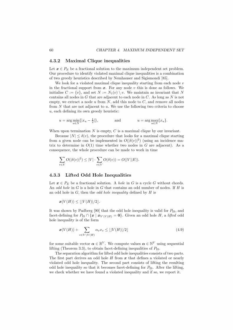
60 CHAPTER 4. MAXIMUM INDEPENDENT SET
4.3.2 Maximal Clique inequalities
Let x ∈ PE be a fractional solution to the maximum independent set problem.Our procedure to identify violated maximal clique inequalities is a combinationof two greedy heuristics described by Nemhauser and Sigismondi [85].
We look for a violated maximal clique inequality starting from each node vin the fractional support from x. For any node v this is done as follows. Weinitialise C := {v}, and set N := N1(v) \ v. We maintain as invariant that Ncontains all nodes in G that are adjacent to each node in C. As long as N is notempty, we extract a node u from N , add this node to C, and remove all nodesfrom N that are not adjacent to u. We use the following two criteria to chooseu, each defining its own greedy heuristic:
u = arg minu∈N{|xu − 1
2 |}, and u = arg maxu∈N{xu}.
When upon termination N is empty, C is a maximal clique by our invariant.Because |N | ≤ δ(v), the procedure that looks for a maximal clique starting
from a given node can be implemented in O(|δ(v)|2) (using an incidence ma-trix to determine in O(1) time whether two nodes in G are adjacent). As aconsequence, the whole procedure can be made to work in time∑
v∈VO(|δ(v)|2) ≤ |V | ·
∑v∈V
O(δ(v)) = O(|V ||E|).
4.3.3 Lifted Odd Hole Inequalities
Let x ∈ PE be a fractional solution. A hole in G is a cycle G without chords.An odd hole in G is a hole in G that contains an odd number of nodes. If H isan odd hole in G, then the odd hole inequality defined by H is
x(V (H)) ≤ b|V (H)|/2c.
It was shown by Padberg [90] that the odd hole inequality is valid for PIS, andfacet-defining for PIS ∩ {x | xV \V (H) = 0}. Given an odd hole H, a lifted oddhole inequality is of the form
x(V (H)) +∑
v∈V \V (H)
αvxv ≤ b|V (H)|/2c (4.9)
for some suitable vector α ∈ RV . We compute values α ∈ NV using sequentiallifting (Theorem 3.3), to obtain facet-defining inequalities of PIS.
The separation algorithm for lifted odd hole inequalities consists of two parts.The first part derives an odd hole H from x that defines a violated or nearlyviolated odd hole inequality. The second part consists of lifting the resultingodd hole inequality so that it becomes facet-defining for PIS. After the lifting,we check whether we have found a violated inequality and if so, we report it.

4.3. A BRANCH-AND-CUT ALGORITHM 61
v0 v1
vk vk−1
vi−1vi
vi+1
vj−1
vj
vj+1
e1
ejej+1
ei
ei+1
{vi , v
j }
ek
Figure 4.2: Identifying an odd hole in a closed walk.
Identifying a (Nearly) Violated Odd Hole Inequality
We start by describing the separation algorithm for the basic odd hole inequal-ities x(V (H)) ≤ b|V (H)|/2c given the vector x. We first find an odd cyclestarting from some node v ∈ V using the construction described by Grotschel,Lovasz, and Schrijver [55]. To find a shortest odd cycle containing node v,Grotschel et al. construct an auxiliary bipartite graph G = ((V 1, V 2), E)and cost vectors c ∈ [0, 1]E and c ∈ [0, 1]E as follows. Each node v ∈ Vis split into two nodes v1 and v2, with vi included in V i (i = 1, 2). Foreach edge {u, v} ∈ E, we add the edges {u1, v2} and {u2, v1} to E, and setc{u,v} = c{u1,v2} = c{u2,v1} = 1 − xu − xv. Observe that a path from u1 ∈ V 1
to v2 ∈ V 2 in G corresponds to a walk of odd length in G from u to v.A shortest path from v1 to v2 in G corresponds to a shortest odd length closed
walk in G containing v. The reason that we are looking for a shortest path isthat an odd hole H in G defines a violated odd hole inequality if c(E(H)) < 1,and a short closed walk in G is more likely to lead to a violated lifted odd holeinequality than a long one. In our implementation, we restricted ourselves toshortest paths with length at most 1.125. Shortest paths in a graph with non-negative edge lengths can be found using Dijkstra’s algorithm [42]. Hence, wecan find a closed walk
C := (v = v0, e1, v1, e2, v2, . . . , vk−1, ek, vk = v)
in G with odd k that is minimal with respect to c and |C| by using Dijkstra’salgorithm to find a shortest path (with respect to c) of minimal cardinality fromv1 to v2 in G. Some of the vi may occur more than once, and the walk mayhave chords.
Let j ∈ 2, . . . , k − 1 be the smallest index such that there exists an edge{vi, vj} ∈ E for some i ∈ 0, . . . , j − 2 (such i, j exist because {v0, vk−1} ∈ E).Let i ∈ 0, . . . , j − 2 be the largest index such that {vi, vj} ∈ E. Let
H := (vi, ei+1, vi+1, . . . , ej , vj , {vj , vi}, vi).

62 CHAPTER 4. MAXIMUM INDEPENDENT SET
The construction of H is illustrated in Figure 4.2. We proceed by showingthat H is indeed an odd hole.
Proposition 4.11. Let H be constructed as above. Then, H is an odd hole inG.
Proof. Because {v1, v2} /∈ E, we have that |H| ≥ 3. Clearly H is a cycle in G.By choice of i and j, H does not contain chords, so H is a hole in G. It remainsto prove that |V (H)| (= j− i+ 1) is odd. Suppose by way of contradiction that|V (H)| is even. Then,
C ′ := (v = v0, e1, . . . , vi−1, ei, vi, {vi, vj}, vj , ej+1, vj+1, . . . , ek, vk = v)
is an odd length closed walk in G containing v. Moreover,
c({ei+1, . . . , ej}) = (j − i)− (2∑j−1p=i+1 xvp)− xvi − xvj .
It follows from x({vp, vp+1}) ≤ 1 that
j−1∑p=i+1
xvp ≤ (j − i− 1)/2.
Therefore,
c({ei+1, . . . , ej}) ≥ (j − i)− (j − i− 1)− xvi − xvj = c{vi,vj},
so C ′ is not longer than C with respect to c. However, C ′ is of smaller cardi-nality, which contradicts our choice of C. Hence H is an odd hole in G.
If |V (H)| = 3, then H is a clique in G, and we ignore it in our computations.
Lifting an Odd Hole Inequality
Let H be an odd hole in G. Assume that we have an ordering of the node setV \ V (H) that is given by {v1, v2, . . . , v|V \V (H)|}. By Theorem 3.3 a lifted oddhole induces a facet if we choose
αvi = b|V (H)|/2c −max{x(V (H)) +∑i−1j=1 αvjxvj | x ∈ Xi
IS},
where
XiIS = {χI | I is an independent set in G[(V (H) ∪ {v1, . . . , vi−1}) \N1(vi)]}.
In order to compute the lifting coefficients, we have to compute several maximumweight independent sets, one for each lifting coefficient.
Nemhauser and Sigismondi [85] observed that αv = 0 for v ∈ V \ V (H) if|N1(v) ∩ V (H)| ≤ 2. This implies that the independent set problems that haveto be solved in order to compute the lifting coefficients α are relatively small inpractice. We lift the variables in non-decreasing lexicographic order of the pairs(| 12 − xv|,−|N1(v) ∩ V (H)|), where ties are broken at random.
To compute the coefficients α, we will make use of a path decomposition(see Bodlaender [19], and de Fluiter [46]) of the graph induced by the nodes inthe hole and the nodes we already lifted.

4.3. A BRANCH-AND-CUT ALGORITHM 63
Definition 4.3. A path decomposition of a graph G = (V,E) is a sequence(Si)ni=1 satisfying the following conditions:⋃n
i=1 Si = V , (4.10)for all {u, v} ∈ E there exists i ∈ {1, . . . , n} with {u, v} ⊆ Si, and (4.11)for all i, j, k with 1 ≤ i < j < k ≤ n we have Si ∩ Sk ⊆ Sj . (4.12)
The width of a path decomposition (Si)ni=1 is the value maxni=1 |Si| − 1.
We may assume without loss of generality that Si and Si+1 differ in onlyone node, i.e., that Si+1 = Si ∪ {v} or Si+1 = Si \ {v} for some v ∈ V .We may also assume without loss of generality that S1 = Sn = ∅. A pathdecomposition satisfying these assumptions is called normalised. A normalisedpath decomposition has n = 2|V |+1. We will present our algorithm to computethe maximum weight of an independent set given a path decomposition in thenext sub-section. Here, we proceed by outlining how we obtain and maintainthe path decomposition that we use for this purpose.
Given a hole H = (v0, e1, v1, . . . , en, vn = v0), an initial path decompositionof the graph G[V (H)] = (V (H), E(H)) of width two is given by
Si =
∅, if i = 1 or i = 2|V (H)|+ 1,{v0}, if i = 2 or i = 2|V (H)|,{v0, vk}, if 2 < i < 2|V (H)| and i = 2k + 1,{v0, vk, vk+1}, if 2 < i < 2|V (H)| and i = 2(k + 1).
Suppose at some stage we want to compute the lifting coefficient for some nodev ∈ V . Let V ′ be the set of nodes that are either in the hole or did alreadyreceive a positive lifting coefficient at some earlier stage. Assume that (Si)
2|V ′|+1i=1
is a path decomposition of the graph induced by V ′. A path decomposition ofG[V ′\N1(v)] can be obtained from (Si)
2|V ′|+1i=1 by eliminating the nodes in N1(v)
from all sets Si (i = 1, . . . , 2|V ′|+ 1) and eliminating consecutive doubles (i.e.,sets Si and Si+1 that are equal).
For each node that we assign a positive lifting coefficient, we have to updateour path decomposition. Suppose at some stage we have found a strictly positivelifting coefficient for some node v ∈ V . Let V ′, (Si)
2|V ′|+1i=1 be as before. We have
to extend the path decomposition so that it becomes a path decomposition forG[V ′ ∪ {v}]. We do this in a greedy fashion, by identifying the indices j, ksuch that j = min{i | {u, v} ∈ E, u ∈ Si} and k = max{i | {u, v} ∈ E, u ∈Si}, and adding v to all sets Si for i ∈ {j, . . . , k}. Having done this, ourpath decomposition satisfies conditions (4.10)–(4.12) for the graph G[V ′ ∪ {v}].We normalise the resulting path decomposition to ensure that it satisfies ourassumptions on the differences between consecutive sets.
Weighted Independent Sets by Path Decomposition
Suppose we are given a graph G = (V,E), together with a normalised pathdecomposition (Si)
2|V |+1i=1 of G. Let I again denote the collection of all inde-

64 CHAPTER 4. MAXIMUM INDEPENDENT SET
pendent sets in G, and let Ii = {I ∈ I | I ⊆ Si} be all independent sets inG[Si]. Finally, let Vi =
⋃ij=1 Sj . Since the path decomposition (Si)
2|V |+1i=1 is
normalised, for all i > 1 there is a node v ∈ V such that either Si = Si−1 ∪ {v}or Si = Si−1 \ {v}. As a consequence the sets Ii satisfy the following recursiverelation:
Ii =
{∅}, if i = 1,Ii−1 ∪ {(I ∪ {v}) ∈ I | I ∈ Ii−1}, if i > 1 and Si = Si−1 ∪ {v}, and{I ∈ Ii−1 | v /∈ I} if i > 1 and Si = Si−1 \ {v}.
(4.13)
Given a path decomposition (Si)2|V |+1i=1 of G and a weight vector α ∈ NV , we
can compute the weight of a maximum weight independent set in G with respectto α using a dynamic programming-like algorithm. To describe this algorithm,we use the functions
zi : Ii → N : I 7→ max{α(I ′) | I ′ is independent set in G[Vi], I ′ ∩ Si = I}.
It follows from condition (4.10) that the value of z2|V |+1(∅) is the maximumweight of an independent set of G, which is what we want to compute. Fromthe definition of zi we find z1(∅) = 0. Now suppose i > 1, let I ∈ I be anindependent set in Si, and let I∗ be the maximum weight independent set inG[Vi] with I∗ ∩Si = I. In the following, we will relate I∗ to a maximum weightindependent set I ′ in G[Vi−1] and characterise I ′ ∩ Si−1. There are four casesto consider.
Case (i): Si = Si−1 ∪ {v} and v /∈ I. Clearly, I∗ also is a maximum weightindependent set in G[Vi−1] with I∗∩Si−1 = I. Hence we can take I ′ = I∗,and I ′ ∩ Si−1 = I.
Case (ii): Si = Si−1 ∪ {v} and v ∈ I. We claim that u ∈ Si for all {u, v} ∈E(Vi). It follows from this claim that I ′ = I∗ \ {v} is a maximum weightindependent set in G[Vi−1] (or I∗ would not be optimal either), and I ′ ∩Si−1 = I \ {v}. To prove our claim suppose by way of contradiction that{u, v} ∈ E(Vi) but u /∈ Si. From this it follows that u ∈ Sk for somek < i. By condition (4.11) there exists j ∈ {1, . . . , 2|V | + 1} such that{u, v} ⊆ Sj . Since Si = Si−1∪{v} and by condition (4.12) v occurs only inconsecutive sets in the path decomposition, we find that j > i. However,condition (4.12) together with u ∈ Sk and u ∈ Sj implies that u ∈ Si, acontradiction, completing the proof of the claim.
Case (iii): Si = Si−1 \ {v} and I ∪{v} is an independent set in G[Si−1]. FromVi = Vi−1 it follows that I ′ = I∗ is a maximum weight independent set inG[Vi−1] with I ′∩Si = I. Either v ∈ I ′ or v /∈ I ′. Hence, I ′∩Si−1 = I∪{v}or I ′ ∩ Si−1 = I.

4.3. A BRANCH-AND-CUT ALGORITHM 65
Case (iv): Si = Si−1 \ {v} and I ∪ {v} is not an independent set in G[Si−1].Since I∗ ∩ Si = I implies (I∗ ∪ {v}) ∩ Si−1 = I ∪ {v}, and I∗ is anindependent set, we have v /∈ I∗. It follows that we can take I ′ = I∗, andI ′ ∩ Si−1 = I.
The case analyses above leads to the following recurrence for zi(I) with i > 1:
zi(I) =
zi−1(I) if Si = Si−1 ∪ {v} and v /∈ I,zi−1(I \ {v}) + αv, if Si = Si−1 ∪ {v} and v ∈ I,max(zi−1(I), zi−1(I ∪ {v})), if Si = Si−1 \ {v} and I ∪ {v} ∈ Ii−1,zi−1(I), if Si = Si−1 \ {v} and I ∪ {v} /∈ Ii−1.
(4.14)
The dynamic programming algorithm works in 2|V | + 1 iterations, num-bered 1, . . . , 2|V | + 1. In iteration i, the algorithm computes the domain of zi,together with its function values. The domain of z1 is {∅}, and z1(∅) = 0. Fori > 1, the domains and function values are computed unfolding the recursivedefinitions (4.13) and (4.14), respectively.
To implement the dynamic programming algorithm, we maintain a list Lof tuples (I, zi(I)) with I ∈ Ii, where i is the iteration number. Iteration 1 isimplemented by setting L = {(∅, 0)}. Iteration i > 1 is implemented as follows.Either Si = Si−1 ∪ {v} or Si = Si−1 \ {v}. If Si = Si−1 ∪ {v} we update L byadding the tuple (I ∪{v}, z+αv) to L for each tuple (I, z) ∈ Li−1 that satisfiesN1(v) ∩ I = ∅. If Si = Si−1 \ {v}, we update L by removing all tuples (I, z)that have v ∈ I. After removing a tuple (I, z) from L, we replace the tuple(I \ {v}, z′) ∈ L by the tuple (I \ {v},max(z, z′)).
If we order L such that for all pairs of tuples (I1, zi(I1)), (I2, zi(I2)) ∈ Lwith I2 ⊂ I1 we have that the tuple containing I1 precedes the tuple containingI2 in L, each iteration can be implemented by a single pass over L, using twopointers into L. If the path decomposition (Si)
2|V |+1i=1 has width w, then the
independent sets in the domains of each of the functions zi can be implementedusing bit vectors of length w, and the ordering can be implemented using the de-fault “greater than” comparison operator on bit vectors. If we restrict ourselvesto path decompositions with width at most 32, then bit vectors can be imple-mented using integers. In that case the dynamic programming algorithm can beimplemented using a double-linked list of tuples of integers as most complicateddata structure.
Proposition 4.12. A maximum weight independent set can be computed usinga path decomposition of width w in O(w2w|V |+ |E|) time.
Proof. When adding a node v, we have to check whether I ∪ {v} ∈ I for each(I, z) ∈ L. This can be done in constant time for each such I after we markthe neighbours of node v. Making a new independent set takes at most O(w)time. It follows that iteration i in which a node is added can be implemented inO(w|Ii| + |δ(v)|), where v is the node we add. If we delete a node in iteration

66 CHAPTER 4. MAXIMUM INDEPENDENT SET
i, all checks and updates can be done in constant time, so the iteration can beimplemented in O(|Ii|) time. Since |Ii| ≤ 2w for all i, the dynamic programmingalgorithm can be implemented to work in
2|V |+1∑i=1
O(w2w + |δ(v)|) = O(w2w|V |+ |E|)
time.
The factor 2w in the time complexity of the dynamic programming algorithmlooks rather ominous. However, the actual running time depends on the actualsize that L attains. In iteration i, this size equals the number of independent setsin G[Si]. In our implementation, we restricted ourselves to path decompositionswith width at most 24, and it rarely occurred that the path width exceeded 24.On those rare occasions, however, we do not compute the true lifting coefficientsbut use a coefficient of 0 instead. Counting to 224 each time we want to computea lifting coefficient would definitely stall our algorithm. Although we cannotexclude the possibility that this occurs, we would like to stress that this didnot occur in our computational experiments. We see this as an indication thatthe worse case behaviour is unlikely to manifest itself on the classes of probleminstances that we are interested in.
4.3.4 Maximally Violated Mod-k Cuts
Suppose x∗ ∈ PE is a fractional solution to the maximum independent set prob-lem. We use the algorithm of Section 3.3.5 to search maximally violated mod-kcuts. As input to the mod-k separation algorithm, we use all (globally) valid in-equalities for PIS that are present in the formulation of the linear programmingrelaxation and are satisfied with equality by x∗. The inequalities we use are thefollowing: maximal clique inequalities (4.2), lifted odd hole inequalities (4.9),non-negativity constraints on xV , upper bound constraints of 1 on componentsof xV , and mod-k cuts that were found at an earlier stage of the algorithm.
4.3.5 Logical Implications
In each node of the branch-and-bound tree we solve a linear programming re-laxation of the form
z∗ = max{z(x) = x(V ) | Ax = b, l ≤ x ≤ u}, (4.15)
for some l,u ∈ {0, 1}V where A, b are obtained from the constraint matrix ofPGUBC and 1, respectively, by adding the rows and right hand sides of valid
inequalities that are produced by our separation algorithms. Recall the notionof setting variables from Section 3.2.2.
We start with the most elementary of all logical implications:

4.3. A BRANCH-AND-CUT ALGORITHM 67
Proposition 4.13. Let v ∈ V be a node in G and let W = N(v) be its set ofneighbours. If xv is set to one, then xw can be set to zero for all w ∈W withoutchanging z∗.
Proof. Directly from the definition of PE .
Proposition 4.14. Let v,W be as in Proposition 4.13. If xw is set to zero forall w ∈W , then xv can be set to one without changing the value of z∗.
Proof. Because z∗ = z(x∗) for some optimal solution x∗ to model (4.15), andx∗W = 0 together with optimality of x∗ implies that x∗v = 1, the propositionholds.
If we set xv to one for some v ∈ V , then we can set xw to zero for allneighbours w of v by Proposition 4.13. In a formulation of the independentset problem with explicit slack variables, such as model (4.4), it is possible tointerpret the slack variable sC that is associated with clique C ∈ C as a variablethat is associated with an extra node that is connected to all nodes in C. Usingthis interpretation we can also apply Proposition 4.13 to the slack variables sCfor all C ∈ C. If we set xv to zero for some v ∈ V , its neighbours may satisfythe conditions of Proposition 4.14.
After applying Proposition 4.13 to all nodes that are set to one, we can re-state the linear programming problem 4.15 in terms of its free variables. Theresulting linear programming problem can be interpreted as a (fractional) in-dependent set problem in the graph induced by the nodes that correspond tothe free variables (i.e., with a lower bound of 0 and an upper bound of 1).Therefore, setting variables to zero can be interpreted as removing nodes fromthe graph.
Proposition 4.15. Let v ∈ G, U = N(v) the set of neighbours of v, and W =N(N1(v)) the set of neighbours of the 1-neighbourhood of v. When removing vfrom G, the following cases can occur:
(i) the nodes in U may become simplicial nodes,
(ii) the nodes in W may become node-dominated by nodes in U , or
(iii) the nodes in W may become set-dominated.
Proof. Directly from Propositions 4.7, 4.8, and 4.9.
After setting a variable to zero, we check whether any of the three cases ofProposition 4.15 occurs, and if so, we take the appropriate action.
4.3.6 Branching Scheme
We complete the description of our branch-and-cut algorithm by giving thebranching scheme we use. Since we use the formulation of the maximum in-dependent set problem with explicit slack variables (4.4) all maximal clique

68 CHAPTER 4. MAXIMUM INDEPENDENT SET
Name Heuristic SectionO1 1-Opt starting from zero 4.2.3O2 1-Opt followed by 2-opt starting from zero 4.2.3L1 Simple LP rounding followed by 1-opt 4.2.1, 4.2.3L2 Simple LP rounding followed by 1-opt and 2-opt 4.2.1, 4.2.3R1 Minimum regret rounding with parameter t = 1 4.2.2R2 Minimum regret rounding with parameter t = 2 4.2.2
Table 4.1: Heuristics for the Maximum Independent Set Problem
inequalities are GUB constraints. We try to take advantage of this by usingbranching on variables and branching on GUB constraints. Deciding whetherto branch on a variable or a GUB constraint is done based on pseudo-cost asdescribed in Section 3.2.5.
4.4 Computational Results
In this section we report on the computational behaviour of the algorithmsproposed in this chapter, which we implemented using the graph data structurefrom LEDA [83]. We tested our algorithms on independent set problems that aresimilar to those reported on in the literature. An interesting class of independentset problem instances that can be found in the literature is the class defined onso-called uniform random graphs, or URGs. URGs are graphs on n nodes inwhich each of the n(n − 1)/2 possible arcs is present with a fixed probabilityp. All averages reported in this section are taken over 25 randomly generatedinstances for every choice of n and p. We will first consider the performance ofour heuristic algorithms, and then proceed by discussing the behaviour of ouroptimisation algorithms.
Heuristics. The heuristics for the maximum independent set problem pre-sented in Section 4.2 are summarised in Table 4.1. The average sizes of themaximum independent sets computed by our heuristics and the correspondingrunning times are reported on in Table 4.2. The columns O1 and O2 refer to theiterative improvement algorithms that were presented in Section 4.2.3. Thesealgorithms use the 1-opt and 2-opt neighbourhoods, respectively, starting from0. The L1, L2, R1 and R2 columns all refer to LP-based rounding algorithmsthat first compute the optimal solution to an LP relaxation of the independentset polytope that is strengthened by our cutting plane routines. The L1 and L2columns refer to the algorithms that first apply the simple LP rounding algo-rithms from Section 4.2.1 to obtain an integer solution. Next, they invoke aniterative improvement algorithm starting from this integer solution using the1-opt and 2-opt neighbourhoods, respectively. The R1 and R2 columns refer toalgorithms that apply the minimum regret rounding heuristic from Section 4.2.2to the optimal solution of the LP relaxation, with the parameter t equal to 1

4.4. COMPUTATIONAL RESULTS 69
O1 O2 L1 L2 R1 R2
n p α CPU α CPU α CPU α CPU α CPU α CPU α(G)
80 .1 21.5 0.0 24.3 0.0 25.2 0.0 26.3 0.0 26.8 0.0 27.0 0.1 27.3.2 13.7 0.0 15.2 0.0 14.5 0.0 15.6 0.0 16.7 0.0 16.8 0.3 18.0.3 9.6 0.0 11.2 0.0 9.7 0.0 11.2 0.0 12.7 0.0 12.7 0.4 13.4.4 8.0 0.0 8.8 0.0 8.0 0.0 8.8 0.0 9.7 0.0 10.1 0.4 10.6.5 6.0 0.0 6.9 0.0 6.0 0.0 6.9 0.0 8.2 0.0 8.3 0.4 8.8.6 4.9 0.0 5.6 0.0 4.9 0.0 5.6 0.0 6.7 0.0 6.9 0.4 7.2.7 3.8 0.0 4.6 0.0 3.8 0.0 4.6 0.0 5.3 0.0 5.5 0.3 5.9.8 3.1 0.0 3.9 0.0 3.2 0.0 4.0 0.0 4.4 0.0 4.5 0.2 4.8.9 2.4 0.0 3.0 0.0 3.6 0.0 3.7 0.0 3.7 0.0 3.7 0.0 3.7
90 .1 21.9 0.0 25.2 0.0 25.8 0.0 27.8 0.0 28.4 0.0 28.7 0.2 29.3.2 14.3 0.0 16.0 0.0 14.5 0.0 16.2 0.0 18.3 0.0 18.4 0.5 19.1.3 9.9 0.0 11.6 0.0 10.0 0.0 11.6 0.0 12.9 0.0 13.1 0.6 14.2.4 7.7 0.0 8.8 0.0 7.7 0.0 8.8 0.0 10.2 0.0 10.4 0.6 11.2.5 6.4 0.0 7.3 0.0 6.4 0.0 7.3 0.0 8.1 0.0 8.0 0.6 9.1.6 5.0 0.0 5.8 0.0 5.0 0.0 5.8 0.0 6.9 0.0 7.0 0.6 7.4.7 4.0 0.0 4.8 0.0 4.0 0.0 4.8 0.0 5.6 0.0 5.8 0.5 6.1.8 3.2 0.0 3.6 0.0 3.2 0.0 3.6 0.0 4.4 0.0 4.6 0.3 4.8.9 2.4 0.0 3.0 0.0 3.8 0.0 3.8 0.0 3.8 0.0 3.8 0.0 3.8
100 .1 23.1 0.0 26.2 0.0 25.8 0.0 27.9 0.0 29.4 0.0 29.5 0.3 30.4.2 14.4 0.0 16.3 0.0 14.6 0.0 16.6 0.0 18.3 0.0 18.9 0.7 19.8.3 10.4 0.0 12.1 0.0 10.4 0.0 12.2 0.0 13.6 0.0 13.7 0.9 14.7.4 8.4 0.0 9.2 0.0 8.4 0.0 9.2 0.0 10.5 0.0 10.8 0.9 11.4.5 6.2 0.0 7.3 0.0 6.2 0.0 7.3 0.0 8.4 0.0 8.6 1.0 9.2.6 5.1 0.0 6.0 0.0 5.1 0.0 6.0 0.0 6.9 0.0 7.1 0.9 7.6.7 4.0 0.0 4.8 0.0 4.0 0.0 4.8 0.0 5.7 0.0 5.6 0.8 6.1.8 3.3 0.0 4.1 0.0 3.3 0.0 4.1 0.0 4.4 0.0 4.5 0.6 5.0.9 2.6 0.0 3.0 0.0 3.7 0.0 3.7 0.0 3.9 0.0 3.9 0.1 4.0
110 .1 24.4 0.0 28.0 0.0 27.2 0.0 29.6 0.0 31.1 0.0 31.1 0.4 32.3.2 14.7 0.0 17.1 0.0 15.0 0.0 17.2 0.0 19.1 0.0 19.1 1.1 20.6.3 11.1 0.0 12.0 0.0 11.1 0.0 12.0 0.0 13.7 0.0 13.9 1.3 15.0.4 8.5 0.0 9.6 0.0 8.5 0.0 9.6 0.0 10.7 0.0 10.8 1.4 11.7.5 6.6 0.0 7.6 0.0 6.6 0.0 7.6 0.0 8.5 0.0 8.9 1.4 9.4.6 5.2 0.0 6.0 0.0 5.2 0.0 6.0 0.0 7.0 0.0 7.0 1.3 7.8.7 4.4 0.0 5.0 0.0 4.4 0.0 5.0 0.0 5.6 0.0 5.8 1.2 6.1.8 3.4 0.0 4.0 0.0 3.4 0.0 4.0 0.0 4.6 0.0 4.8 0.8 5.0.9 2.8 0.0 3.1 0.0 2.9 0.0 3.2 0.0 3.7 0.0 3.8 0.2 4.0
Table 4.2: Heuristics on Uniform Random Graphs (URGs)

70 CHAPTER 4. MAXIMUM INDEPENDENT SET
and 2, respectively. The α columns contain the average size of the resultingindependent set, the CPU columns contain the average number of CPU secondsthat were needed to find the reported independent sets, the time needed to solvethe LP relaxations excluded. Finally, the α(G) column contains the average sizeof the maximum independent set in the test instances.
On uniform random graphs the 2-opt algorithm consistently performs betterthan the 1-opt algorithm (on average). Using a rounded LP solution as a startingpoint of an iterative improvement algorithm improves the quality of the reportedindependent sets for sparse problems (p ≤ .2) and for dense problems (p = .9).The minimum regret heuristics perform consistently better (on average) than thesimple rounding plus iterative improvement heuristics. All rounding algorithmsare fast in practice (CPU time < .1s on average, with the exception of minimumregret rounding with t = 2 that runs within 1.5s), the CPU time needed for therounding phase is dominated by the CPU time needed for solving the linearprograms. This makes these algorithms well suited for use from within an LPbased branch-and-bound algorithm. Note that the minimum regret heuristicwith parameter t = 2 often achieves an average value of α that is greater thanα(G) − 1. This can only happen if the algorithm reports optimal solutions onsome of the instances.
Optimisation Algorithms. The average performance of our branch-and-cutand cutting plane/branch-and-bound algorithms are presented in Tables 4.3and 4.4, respectively. In our cutting plane/branch-and-bound algorithm wesolve the root node in exactly the same way as we do in our branch-and-cutalgorithm, and then invoke the MIP solver from CPLEX with the strongestpossible formulation and the best primal bound we have available. In thesetables, the Nodes column contains the average number of nodes in the branch-and-bound tree, and the CPU column contains the average CPU time it tookfor the algorithm to terminate in seconds. The remaining columns report onthe effectiveness of the valid inequalities we use, and their corresponding sepa-ration algorithms. For each class of valid inequalities, the # column containsthe average number of distinct valid inequalities that were separated, the Gapcolumn contains the average percentage of duality gap closed in the root node,and the Prof. column contain the average amount of CPU time that was spentin the corresponding separation algorithm (Prof. is an abbreviation of ProfilingData).
When comparing the branch-and-cut algorithm to the cutting plane/branch-and-bound algorithm, it is clear that the faster of the two algorithms is thecutting plane/branch-and-bound algorithm. We believe that this is due to thefact that we use the MIP solver of CPLEX 6.5 for the branch-and-bound phase,which is a highly optimised commercial package. The branch-and-cut algorithmdoes achieve the smallest branch-and-bound tree sizes of on almost all of theruns. From the Gap columns it is clear that using our cutting plane routinesfrom each node in the branch-and-bound tree does improve the formulation.Here, maximum clique inequalities become more important when problems are

4.4. COMPUTATIONAL RESULTS 71
Performance Max Clique Lifted Odd Hole Mod-k
n p Nodes CPU # Gap Prof. # Gap Prof. # Gap Prof.
80 .1 9.2 55.6 221.7 0.3 0.6 220.0 59.0 2.2 121.3 43.8 33.6.2 87.3 187.2 425.4 5.1 1.1 327.1 19.7 4.1 423.7 9.1 32.8.3 139.6 235.4 702.0 11.8 1.1 92.7 6.3 5.0 364.1 7.6 25.0.4 110.2 309.5 997.2 21.0 1.1 22.8 3.2 5.5 333.8 11.8 20.8.5 67.8 350.8 1223.3 34.2 1.0 4.7 1.7 3.8 250.8 22.6 17.2.6 42.2 378.6 1278.6 48.2 0.8 1.0 0.8 2.4 175.9 33.4 15.6.7 18.4 363.8 1302.5 62.2 0.6 0.5 1.3 1.9 114.9 46.7 15.2.8 4.5 178.2 1038.8 75.6 0.5 0.0 0.0 1.9 53.6 49.2 15.3.9 1.0 15.6 634.4 75.6 1.2 0.0 0.0 5.1 15.2 31.9 50.1
90 .1 16.9 108.7 273.6 0.5 0.6 351.4 51.7 2.5 190.2 33.3 32.6.2 272.4 464.6 590.6 5.1 1.4 692.1 20.5 5.4 1033.7 6.4 39.0.3 354.5 656.1 1095.9 13.3 1.2 214.2 7.9 5.8 876.6 7.4 27.3.4 218.0 748.8 1590.7 21.8 1.2 36.4 3.2 5.6 644.4 12.7 21.4.5 131.9 737.2 1794.7 34.4 0.9 3.2 1.0 3.5 382.2 21.2 16.4.6 72.3 1023.6 2223.4 47.1 0.7 0.6 0.6 2.2 323.2 33.6 13.5.7 30.0 861.2 2002.0 61.4 0.5 0.1 0.5 1.7 184.2 47.1 12.2.8 8.0 520.1 1513.3 73.6 0.4 0.1 0.3 1.5 87.6 52.6 14.1.9 1.0 29.5 886.5 78.5 1.1 0.0 0.0 5.7 22.2 44.0 53.0
100 .1 65.5 339.2 333.4 0.6 1.0 997.4 41.1 4.5 767.5 23.5 46.7.2 766.6 1000.0 844.5 5.7 1.3 992.0 16.9 5.6 1611.5 4.6 33.1.3 1008.0 1965.0 1675.2 12.3 1.0 376.9 7.5 5.3 1649.8 6.1 21.5.4 712.8 3042.3 2767.4 21.9 1.0 86.6 5.1 4.6 1557.5 11.9 16.7.5 244.8 1802.0 2813.0 34.5 0.8 4.8 0.9 3.1 625.2 22.0 14.4.6 133.6 2047.8 3085.8 47.1 0.7 1.4 0.5 2.2 473.6 33.4 13.2.7 54.8 1749.1 2867.4 58.6 0.5 0.1 0.0 1.9 282.0 43.8 12.2.8 7.3 1255.6 2087.6 74.4 0.3 0.0 0.0 1.2 106.7 56.1 8.1.9 1.3 183.9 1289.4 86.1 0.5 0.0 0.0 2.6 38.9 59.4 19.4
110 .1 213.6 808.4 395.4 0.8 1.2 2114.0 40.7 5.5 1816.4 21.2 53.8.2 2542.4 3309.3 1210.0 5.3 1.0 1883.0 16.5 5.0 3564.9 3.7 26.1.3 2528.7 5230.9 2370.5 12.3 0.7 506.7 6.6 3.7 2354.7 5.6 14.2.4 1291.7 4984.3 3392.5 22.3 0.7 76.0 3.7 3.4 1510.9 12.2 12.0.5 564.9 5564.0 4763.7 34.8 0.7 18.6 3.0 2.6 1301.1 21.7 12.3.6 210.4 3935.6 4699.5 46.9 0.7 1.0 0.7 2.1 727.6 32.3 12.7.7 82.5 3770.2 4562.8 58.0 0.5 0.2 0.2 1.7 479.7 43.9 12.1.8 14.4 2625.8 3174.0 71.6 0.3 0.0 0.0 1.1 181.8 56.8 8.4.9 1.6 691.3 1633.1 83.6 0.2 0.0 0.0 1.1 47.0 54.6 7.9
Table 4.3: Run-Time Behaviour of Branch-and-Cut on URGs

72 CHAPTER 4. MAXIMUM INDEPENDENT SET
Performance Max Clique Lifted Odd Hole Mod-k
n p Nodes CPU # Gap Prof. # Gap Prof. # Gap Prof.
80 .1 21.6 26.3 221.1 0.3 0.4 101.3 53.6 1.4 36.5 41.3 18.4.2 314.2 34.5 348.0 4.7 0.2 6.9 3.8 0.8 11.5 6.4 4.1.3 356.6 59.1 470.2 10.6 0.1 0.2 0.2 0.9 10.1 5.8 2.4.4 231.1 95.5 589.1 18.6 0.2 0.0 0.0 1.3 17.1 9.0 3.4.5 162.7 136.3 706.3 31.2 0.2 0.0 0.0 0.8 20.2 17.6 3.2.6 96.0 179.4 792.6 45.0 0.2 0.0 0.0 0.7 24.4 26.9 3.8.7 66.8 256.3 895.9 59.8 0.2 0.0 0.6 0.7 31.1 40.0 4.3.8 18.8 226.4 874.1 74.3 0.2 0.0 0.0 0.8 28.0 47.1 4.8.9 1.1 59.3 634.3 75.6 0.3 0.0 0.0 1.4 15.2 31.9 13.5
90 .1 75.5 42.3 271.8 0.5 0.3 105.6 42.0 1.2 35.6 27.3 13.7.2 954.7 74.8 429.8 4.7 0.1 4.8 2.2 0.6 13.3 4.8 2.5.3 754.6 134.9 601.5 11.6 0.1 0.0 0.1 0.9 16.9 6.1 2.1.4 402.3 173.2 749.4 19.4 0.2 0.0 0.0 1.0 19.8 10.5 2.6.5 200.8 232.6 892.7 31.4 0.2 0.0 0.0 0.6 22.7 16.4 2.8.6 117.9 351.4 1044.5 44.1 0.2 0.0 0.0 0.6 28.9 27.1 3.2.7 89.5 471.4 1139.5 58.7 0.1 0.0 0.0 0.6 34.3 39.6 3.4.8 44.9 506.0 1149.9 72.5 0.1 0.0 0.0 0.7 37.2 49.8 4.3.9 1.4 118.2 886.5 78.5 0.3 0.0 0.0 1.4 22.2 44.0 13.6
100 .1 415.2 63.3 327.6 0.6 0.2 96.0 28.1 1.0 32.0 17.5 8.8.2 1769.2 146.7 539.0 4.9 0.1 1.9 0.7 0.4 10.4 3.2 1.3.3 1426.6 269.2 740.0 10.6 0.1 0.0 0.0 0.8 18.9 4.9 1.5.4 679.0 314.6 929.5 19.8 0.1 0.0 0.0 0.8 21.6 9.3 1.9.5 323.6 417.5 1118.0 31.2 0.1 0.0 0.0 0.5 26.0 17.4 2.3.6 179.1 582.2 1255.2 43.2 0.1 0.0 0.0 0.5 29.3 27.2 2.5.7 122.3 798.3 1386.9 55.5 0.1 0.0 0.0 0.6 38.2 36.9 3.6.8 70.7 864.6 1427.4 72.5 0.1 0.0 0.0 0.6 35.7 51.6 3.8.9 1.3 431.0 1261.3 86.0 0.2 0.0 0.0 1.0 36.0 59.0 7.1
110 .1 901.9 99.2 384.4 0.7 0.2 88.9 23.0 0.7 28.7 14.4 5.1.2 3786.0 324.1 641.2 4.2 0.0 0.8 0.2 0.3 10.4 2.3 0.7.3 3070.0 496.6 877.5 10.5 0.0 0.0 0.0 0.5 15.1 4.1 0.8.4 1505.6 541.4 1130.8 19.6 0.1 0.0 0.0 0.5 21.3 9.2 1.4.5 566.1 615.9 1337.4 31.1 0.1 0.0 0.0 0.5 26.2 16.3 2.2.6 266.3 777.9 1501.2 42.6 0.1 0.0 0.0 0.5 29.8 24.8 2.5.7 149.4 1107.2 1723.9 55.0 0.1 0.0 0.0 0.6 44.6 37.9 3.5.8 118.7 1256.0 1790.6 69.6 0.1 0.0 0.0 0.6 38.8 50.7 3.7.9 12.0 828.1 1542.6 83.3 0.1 0.0 0.0 0.7 38.4 53.8 4.9
Table 4.4: Run-Time Behaviour of Cutting-Plane/Branch-and-Bound on URGs

4.4. COMPUTATIONAL RESULTS 73
more dense, lifted odd hole inequalities become more important for problemswith lower densities, and mod-k cuts do well for p = .1 and p ≥ .5.
When comparing the branch-and-bound tree sizes of our branch-and-cutalgorithm to those reported in the literature by Mannino and Sassano [80] andSewell [106], it is clear that we achieve the smallest branch-and-bound tree sizesfor very sparse problems (p ≤ .2) and very dense problems (p ≥ .8), even thoughwe do not employ a branching scheme that is tailor-made for the independentset problem. We believe that this is due to the quality of the bound obtainedfrom the strengthened LP relaxations that we use. This quality does have itscost, though, because we spend a lot of time in each node of the branch-and-bound tree to obtain it. As a consequence, our algorithm is outperformed interms of CPU time by those reported on in the literature.
Run time profiles, branching decisions, and the average number of variablesthat is set by our pre-processing, reduced cost and logical implication sub-routines are reported on in Table 4.5. The LP, F, VP, GP, Sep, Set, and Heurcolumns contain the percentage of CPU time spent in solving linear programs,formulating subproblems, initialising and maintaining variable pseudo costs,GUB pseudo costs, variable setting and our rounding heuristics, respectively.The GUB column contains the percentage of branches that were GUB branches,all other branches were variable branches. A minus indicates that all runsof the algorithm that were averaged over were solved in the root node. TheU and L columns contain the average number of variables that were set bystrengthened reduced cost fixing to their upper and lower bound, respectively.The SP, ND, and SD the average number of nodes that were set because theybecame simplicial, node-dominated, and set-dominated, respectively.
The GUB column clearly shows that GUB branches are competitive withvariable branches when compared using pseudo costs. It was to be expectedthat GUB branching would be very useful on the dense instances. Surprisingly,it also is very competitive for the instances with p = .1 and n ≥ 90. The relativelarge amount of time spent in initialising the GUB pseudo costs for problemswith higher density (p ≥ .5) is due to the fact that the branch-and-bound treesizes are small on those classes of instances. Finally, we note that our variablesetting criteria do not have a particularly large yield. On the other hand, theydo not take up a lot of CPU time.

74 CHAPTER 4. MAXIMUM INDEPENDENT SET
Run-Time Profiles Variable Setting
n p LP F VP GP Sep Set Heur GUB U L SP ND SD
80 .1 0.3 3.7 40.5 12.6 36.5 1.9 1.7 7.8 0.0 2.2 0.2 0.4 0.0.2 1.8 6.2 15.9 24.4 37.9 4.2 3.8 22.2 0.0 0.0 0.0 0.0 0.0.3 3.4 8.8 15.0 25.3 31.1 5.6 4.4 18.5 0.0 0.0 0.0 0.0 0.0.4 2.8 10.3 15.8 29.2 27.4 5.6 3.4 24.8 0.0 0.0 0.0 0.0 0.0.5 1.9 10.0 18.3 37.2 21.9 4.1 2.5 25.1 0.0 0.0 0.0 0.0 0.0.6 1.2 7.9 20.3 44.4 18.8 2.9 1.7 19.2 0.0 0.0 0.0 0.0 0.0.7 0.6 5.8 23.6 47.3 17.7 2.3 1.0 21.2 0.0 0.0 0.0 0.0 0.6.8 0.2 4.3 21.0 52.0 17.8 2.3 0.6 31.8 0.0 0.1 0.0 0.0 8.8.9 0.1 9.1 0.0 0.0 56.4 12.2 1.2 − 0.0 15.2 0.0 2.5 24.7
90 .1 0.4 4.1 33.7 18.2 35.8 1.9 2.3 33.2 0.0 0.2 0.2 0.2 0.0.2 3.2 9.5 7.7 13.5 45.7 6.7 5.7 30.4 0.0 0.0 0.0 0.0 0.0.3 4.9 13.5 8.0 16.2 34.3 8.7 5.5 34.3 0.0 0.0 0.0 0.0 0.0.4 3.5 15.4 10.6 23.8 28.1 7.2 4.0 32.6 0.0 0.0 0.0 0.0 0.0.5 2.5 14.7 14.3 34.4 20.9 5.1 2.7 20.9 0.0 0.0 0.0 0.0 0.0.6 1.3 11.0 15.3 47.5 16.4 3.6 1.6 22.6 0.0 0.0 0.0 0.0 0.0.7 0.7 7.0 19.0 53.7 14.4 2.4 1.0 21.8 0.0 0.0 0.0 0.0 0.3.8 0.2 4.6 18.8 56.6 16.0 1.8 0.5 28.4 0.0 0.0 0.0 0.0 7.4.9 0.1 9.9 0.0 0.0 59.7 12.6 0.8 − 0.1 19.9 0.0 1.7 26.0
100 .1 0.7 6.5 13.1 13.0 52.2 3.1 2.9 71.5 0.0 0.0 0.1 0.2 0.0.2 5.9 12.9 4.3 9.6 39.9 8.9 8.7 25.0 0.0 0.0 0.0 0.0 0.0.3 7.4 20.1 4.2 12.0 27.8 10.4 6.7 21.4 0.0 0.0 0.0 0.0 0.0.4 6.2 24.3 5.7 16.8 22.3 9.6 3.9 16.7 0.0 0.0 0.0 0.0 0.0.5 3.1 18.9 11.5 32.6 18.3 6.3 2.6 21.9 0.0 0.0 0.0 0.0 0.0.6 1.7 14.2 14.1 43.4 16.1 4.7 1.5 21.7 0.0 0.0 0.0 0.0 0.0.7 0.7 9.0 16.9 53.2 14.6 2.6 0.9 21.8 0.0 0.0 0.0 0.0 0.0.8 0.1 3.5 17.0 67.6 9.6 1.2 0.4 46.8 0.0 0.0 0.0 0.0 4.7.9 0.0 4.3 10.5 54.4 22.4 4.0 0.3 100.0 0.0 15.0 0.0 0.6 26.1
110 .1 1.2 7.9 5.7 7.7 60.4 4.0 3.6 63.5 0.0 0.0 0.0 0.0 0.0.2 8.7 16.5 1.8 6.8 32.2 10.8 11.3 18.1 0.0 0.0 0.0 0.0 0.0.3 10.9 24.1 2.3 10.0 18.6 12.6 7.6 19.3 0.0 0.0 0.0 0.0 0.0.4 8.7 27.0 4.4 16.0 16.1 10.3 4.8 20.7 0.0 0.0 0.0 0.0 0.0.5 4.8 24.5 8.0 26.1 15.7 8.5 2.3 13.7 0.0 0.0 0.0 0.0 0.0.6 2.2 17.2 12.9 39.8 15.5 5.6 1.4 17.4 0.0 0.0 0.0 0.0 0.0.7 0.8 10.7 15.8 51.5 14.3 3.4 0.8 21.1 0.0 0.0 0.0 0.0 0.0.8 0.2 4.2 14.7 68.6 9.8 1.3 0.4 40.1 0.0 0.0 0.0 0.0 3.3.9 0.0 2.1 6.5 79.0 9.1 1.6 0.1 87.5 0.0 4.0 0.0 0.3 26.5
Table 4.5: Profiles, Branching, and Setting Statistics of Branch-and-Cut

Part II
Applications
75


Chapter 5
Map Labelling
5.1 Introduction
When designing maps, an important question is how to place the names of thecities on the map such that each name appears close to its city and no twonames overlap. Various problems related to this question are referred to asmap labelling problems. We consider a variant of the map labelling problemdescribed in Section 5.1.1. In Section 5.2 we show that this variant of the maplabelling problem reduces to a maximum independent set problem. To solve it tooptimality we slightly refine our optimisation algorithms for finding maximumindependent sets from Chapter 4 for map labelling. In Section 5.3 we presentcomputational results of both our heuristics for finding independent sets fromChapter 4 and our refined optimisation algorithms. Our computational resultsare obtained on graphs derived from an interesting class of randomly generatedmap labelling problem instances that is taken from the literature. We showthat our heuristic algorithms yield close to optimal solutions, and that ouroptimisation algorithms are capable of solving map labelling problem instanceswith up to 950 cities to optimality within reasonable time.
5.1.1 Problem Definition
The basic map labelling problem can be described as follows: given a set P ={p1,p2, . . . ,pn} of n distinct points in R2, determine the supremum σ∗ of allreals σ for which there exist n pairwise disjoint, axis-parallel σ × σ squaresQ1, Q2, . . . , Qn ⊂ R2, where pi is a corner of Qi for all i = 1, . . . , n. By “pairwisedisjoint squares” we mean that no overlap between any two squares is allowed.Once the squares are known, they define the boundaries of the areas where thelabels can be placed. We will refer to this problem as the basic map labellingproblem. The decision variant of the map labelling problem is to decide, for anygiven σ, whether there exists a set of squares Q1, . . . , Qn as described above.Formann and Wagner [47] showed that this latter problem is NP-complete.
77

78 CHAPTER 5. MAP LABELLING
Kucera, Mehlhorn, Preis, and Schwarzenecker [73] observed that there areonly O(n2) possible values that σ∗ can take. Optimising over those can bedone by solving the decision variant only O(logn) times, using binary searchwith different values of σ. So, the basic map labelling problem reduces to thedecision variant. Kucera et al. also present an exponential-time algorithm thatsolves the decision variant of the map labelling problem to optimality. They donot, however, report on successful computational experiments.
Another variant of the map labelling problem, which we will refer to as theoptimisation variant, has the label size σ as input, and asks for as many pairwisedisjoint squares of the desired characteristic as possible. If the number of squaresin an optimal solution to the optimisation variant of the map labelling problemequals n, then this solution is a feasible solution to the decision variant, andvice versa. Hence, the decision variant of the map labelling problem reducesto the optimisation variant via a polynomial reduction. It is the optimisationvariant of the map labelling problem that is the subject of this chapter. Sincethe decision variant is NP-complete, the optimisation variant is NP-hard.
5.1.2 Related Literature
A recent survey on map labelling is given by Neyer [89]. An exhaustive bibliogra-phy concerning map labelling is maintained by Wolff and Strijk [121]. Formannand Wagner [47] developed a 1
2 -approximation algorithm for the optimisationvariant of the map labelling problem. Different heuristic algorithms (includingsimulated annealing) are discussed by Christensen, Marks, and Shieber [27].Van Dijk, Thierens and de Berg [41] considered genetic algorithms, Wagner andWolff [119] propose a hybrid heuristic. Cromly [30] proposed a semi-automaticLP-based approach for finding feasible solutions to the optimisation variant.Zoraster [127, 128] used Lagrangian relaxation to make a heuristic algorithmfor the optimisation variant.
All the results mentioned so far concern the problem in which each point islabelled with one (square) region from a finite set of candidate (square) regions.Kakoulis and Tollis [68] exploit this discrete nature to unify several slightlymore general map labelling problems. A different approach reported on by vanKreveld, Strijk, and Wolff [72] and Klau and Mutzel [71] is to allow a label totake any position, as long as its corresponding point is on its boundary. Thisleads to so-called sliding map labelling models. The advantage of a sliding modelis that more labels can be placed without overlap. In more recent studies alsoother shapes of the label regions are considered (see e.g. Qin, Wolff, Xu andZu [97]).
In this chapter we study the optimisation variant of the basic map labellingproblem. In the remainder of this chapter we will refer to it as the map labellingproblem.

5.2. A BRANCH-AND-CUT ALGORITHM 79
5.2 A Branch-and-Cut Algorithm
In this section, we present our branch-and-cut algorithm for map labelling. Sec-tion 5.2.1 gives the reduction from the map labelling problem to the maximumindependent set problem. The reduction uses the notion of conflict graphs ofmap labelling problem instances. In Section 5.2.2 we show that there are atmost polynomially many maximal cliques in the conflict graph of a map la-belling problem instance, and that these can be found in polynomial time.
Our algorithms for the map labelling problem work with the conflict graphonly, and are therefore applicable to all map labelling problems that can beformulated as maximum independent set problems on conflict graphs. Theproblems that fit in the framework by Kakoulis and Tollis [68] all satisfy this re-quirement. For example, map labelling problems with finite, but more than fourpossible placements of each label, and problems in which the regions occupiedby labels have different (non-uniform) shapes and sizes can all be formulatedas a maximum independent set problems on conflict graphs. Also, it is possi-ble to assign different weights to different label placements, in which case wewould be interested in a maximum weight independent set. We stress that allour algorithms for map labelling can easily be transferred to these more generalmodels. To simplify the discussion and to allow for comparison of our resultswith results reported on in the literature we focus on the special case in whichthere are four possible positions for each label, and the labels are rectangles ofgiven dimensions.
The conflict graphs arising from map labelling problems have a very specialcharacteristic, namely, it is easy to embed them in the plane. In the resultingembedded graphs, nodes are only connected to other nodes that are nearby. Itis this local structure in which the independent set problems arising from maplabelling differ from those for the uniform random graphs studied in Chapter 4.We exploit the special structure in two ways.
It turns out that our routines for setting variables (see Sections 3.2.3, 4.3.1and 4.3.5) are effective for independent set problems in conflict graphs of maplabelling problem instances. In combination with the local structure this createsthe possibility that the sub-graph induced in the conflict graph by the nodescorresponding to free variables can become disconnected in any iteration ofthe branch-and-cut algorithm, even when we start with a connected conflictgraph. In those iterations the associated maximum independent set problemscan be decomposed. We exploit this observation and enhance our branch-and-cut algorithm with a technique that we call variable setting by recursion andsubstitution, which is the subject of Section 5.2.3.
A second way to exploit the local structure in the conflict graphs of map la-belling problems is to be more conservative with calling the separation routines.Especially for large problems this can be a key factor in the effectiveness of abranch-and-cut algorithm. Section 5.2.4 explains how we enhance our branch-and-cut algorithm with this idea.

80 CHAPTER 5. MAP LABELLING
Figure 5.1: A Solution to a Map Labelling Problem on 950 Cities
5.2.1 Reduction from Map Labelling to Independent Set
An instance of the map labelling problem in which the labels are rectangles ofuniform size consists of a finite set of points P ⊂ R2 and a label size σ1 × σ2.In the following, we assume that the label size (σ1, σ2) is fixed. Under thisassumption, an instance of the map labelling problem is completely specified bythe point set P .
For any point p ∈ P , there are four possible placements of a rectangular labelQ such that p is a corner of Q, each occupying a different rectangular region inR2. Denote these rectangular regions by Qpi with i ∈ {1, 2, 3, 4}. Let Q(P ) bethe set of all rectangular regions that correspond to possible label placementsin a solution to the map labelling problem instance P :
Q(P ) = {Qpi | p ∈ P, i ∈ {1, 2, 3, 4}}.
A feasible solution to the map labelling problem instance P is a set of rectan-gular regions S ⊆ Q(P ) such that for any pair of rectangular regions Q,R ∈ Swe have that if Q ∩ R 6= ∅ then Q = R. Note that this definition correctlyprevents a point p ∈ P from having more than one label, as the intersectionof those labels would contain p and would therefore be non-empty. The maplabelling problem is the problem of finding a solution of maximum cardinal-ity. An optimal solution to a map labelling problem on 950 cities is depictedin Figure 5.1. All labelled cities are drawn as black discs, all unlabelled citiesare drawn as black circles. All possible rectangular regions representing a labelposition are shown, those that are coloured grey are part of the solution.

5.2. A BRANCH-AND-CUT ALGORITHM 81
To reduce the map labelling problem to a maximum independent set prob-lem, we will make use of the following notion from graph theory. In the definitionwe will take the more general perspective of sets of regions. Also, vQ alwaysdenotes some node uniquely associated with the region Q.
Definition 5.1. Given a set of regionsQ, the intersection graph GQ = (VQ, EQ)is given by
VQ = {vQ | Q ∈ Q}, and (5.1)EQ = {{vQ, vR} ⊆ VQ | Q ∩R 6= ∅}. (5.2)
Here, (5.1) ensures that for each region in Q there is a node vQ in GQ, and(5.2) ensures that for each pair (Q,R) of intersecting regions in Q there is anedge {vQ, vR} in GQ. Given an instance P of the map labelling problem, wedefine the conflict graph of P as the intersection graph of Q(P ).
Theorem 5.1. Let P ⊂ R2 be an instance of the map labelling problem. Thereis a bijection between the feasible solutions S of P and the independent sets inthe conflict graph of P .
Proof. Suppose that S is a solution of P . Let S ⊆ VQ(P ) be the unique setof nodes of the conflict graph of P that correspond to the labels in S, i.e.S = {vQ | Q ∈ S}. Because S is a solution to P , for any two distinct labelsQ,R ∈ S we have that Q ∩ R = ∅. Hence {vQ, vR} /∈ EQ. It follows that S isan independent set in GQ(P ).
Now, suppose that S is an independent set in GQ(P ). Let S be the unique setof rectangular regions associated with the nodes in S, i.e. S = {Q | vQ ∈ S}.Because S is an independent set in GQ and {vQ, vR} ∈ EQ for all distinctQ,R ∈ Q such that Q ∩ R 6= ∅ we have that Q ∩ R = ∅ for all distinctQ,R ∈ S. Hence S is a solution to P .
An example of a conflict graph of a map labelling instance is depicted inFigure 5.2. The map labelling instance has 250 cities, the conflict graph has1000 nodes. A maximum independent set in the conflict graph is indicated bythe solid nodes.
5.2.2 Finding all Maximum Cliques in the Conflict Graph
Suppose we are given a set Q of axis-parallel rectangular regions in R2. It wasobserved by Imai and Asano [63] that there exists a correspondence betweenthe cliques in GQ and maximal non-empty regions that are contained in theintersection of subsets of regions from Q.
Lemma 5.2. Let Q be a set of axis-parallel rectangular regions. Then, there isa bijection between the cliques in GQ and the non-empty intersections of subsetsof rectangular regions from Q.

82 CHAPTER 5. MAP LABELLING
Figure 5.2: The Conflict Graph of a Map Labelling Problem on 250 Cities
Proof. Let S ⊆ Q be a collection of rectangular regions with non-empty inter-section. Clearly, the rectangular regions in S intersect pairwise. Hence, for eachQ,R ∈ S, {vQ, vR} ∈ EQ. So, the set C = {vQ | Q ∈ S} is a clique in GQ.
Conversely, let C be a clique in GQ, and let S = {Q | vQ ∈ C} be therectangular regions in Q that correspond to the nodes in C. Because C is aclique, all rectangular regions in S intersect pairwise. This implies that the re-gion R =
⋂Q∈S Q is non-empty by the following argument (see e.g. Danzer and
Grunbaum [37]). The intersection of a set of axis-parallel rectangular regions isnon-empty if and only if the intersection of the projections of the rectangularregions on the axis are non-empty. The projections of the rectangular regionson the axes are sets of line-segments in R. By Helly’s theorem, a set of line-segments has a non-empty intersection if and only if all pairs of line-segmentsin the set intersect.
Let C be the collection of all maximal cliques in GQ, and let
R = {⋂vQ∈C Q | C ∈ C}.
It follows from the proof of Lemma 5.2 that R contains all maximal regionsthat are contained in the intersection of a maximal subset of rectangular regionsfrom Q that has a non-empty intersection. The following lemma shows that theregions in R are mutually disjoint.
Lemma 5.3. Let R1, R2 ∈ R. If R1 ∩R2 6= ∅, then R1 = R2.

5.2. A BRANCH-AND-CUT ALGORITHM 83
Proof. Let Si ⊆ Q be the set of rectangular regions such that Ri =⋂Q∈Si Q
(i ∈ {1, 2}), and assume that R1 ∩ R2 6= ∅. Let C = {vQ | Q ∈ S2}. Notethat C is a maximal clique in GQ because R2 ∈ R. Choose Q1 ∈ S1 arbitrarily.Because R1∩R2 6= ∅, also Q1∩R2 6= ∅, which in turn implies that Q1∩Q 6= ∅for all Q ∈ S2. This implies that {vQ1 , vQ} ∈ EQ for all Q ∈ S2 \{Q1}. BecauseC is a maximal clique, this means that vQ1 ∈ C, so Q1 ∈ S2. Since Q1 waschosen arbitrarily, it follows that S1 ⊆ S2. Similarly, we find that S2 ⊆ S1. Thisimplies that S1 = S2 and that R1 = R2.
Recall the clique formulation of the independent set problem on G from Sec-tion 4.1.2. If the clique formulation is derived from the collection of all maximalcliques in G we call it the complete clique formulation. We are interested infinding all maximal cliques in the intersection graph of Q in order to obtainthe complete clique formulation of the independent set problem on GQ. Thefollowing lemma states that the number of maximal cliques in the intersectiongraph of Q is not too large.
Lemma 5.4. The number of maximal cliques in GQ = (VQ, EQ) is at most|VQ|+ |EQ|.
Proof. We will show that there exists an injection f : R → VQ ∪ EQ. Since|R| = |C|, this proves the lemma.
Consider any region R ∈ R. Since R is the intersection of a subset ofrectangular regions from Q we can write R = {x ∈ R2 | l ≤ x ≤ u}, where l1and l2 are determined by the boundary of some rectangular regions Q1, Q2 ∈ Q,respectively. Note that Q1 and Q2 do not have to be unique. Consider any pairQ1, Q2 as above. If Q1 = Q2, we define f(R) to be vQ1 . Otherwise, l ∈ Q1∩Q2,so {vQ1 , vQ2} ∈ EQ, and we define f(R) to be {vQ1 , vQ2}.
It remains to show that f is indeed an injection. Let R1, R2 ∈ R and supposethat f(R1) = f(R2). Let li,ui ∈ R2 be the points such that Ri = {x ∈ R2 |li ≤ x ≤ ui} (for i ∈ {1, 2}). Because f(R1) = f(R2), by construction of f wehave that l1 = l2, so R1∩R2 6= ∅. By Lemma 5.3 we find that R1 = R2. Hencef is an injection.
All single-node components of GQ define their own maximal clique. Asthese maximal cliques can be reported separately, suppose that GQ does nothave isolated nodes. The following algorithm is a brute-force algorithm byStrijk [108] that exploits Lemma 5.3 to find all maximal cliques. For each edge{vQ, vR} ∈ EQ, we compute a maximal clique C that contains a fixed cornerl of Q ∩ R, and then test whether C is a maximal clique in GQ. If this is thecase, we report C, otherwise we proceed with the next edge. Computing C canbe done by testing for each node vS ∈ N({vQ, vR}) whether l ∈ S and if so,adding vS to C. C is a maximal clique in GQ if for each node vS ∈ N({vQ, vR})we have that S ∩
⋂vQ∈C Q = ∅.
Theorem 5.5. The maximal cliques in GQ can be found in O(|VQ||EQ|) time.

84 CHAPTER 5. MAP LABELLING
Proof. The correctness of the brute-force algorithm described above follows di-rectly from Lemma 5.2 and Lemma 5.3. It remains to analyse its time complex-ity. For each edge {u, v} ∈ EQ, the brute-force algorithm described above usesO(|δ(u)| + |δ(v)|) time. Hence, the total time complexity needed for reportingall maximal cliques in GQ is∑{u,v}∈EQ
O(|δ(u)|+ |δ(v)|) = O(∑
{u,v}∈EQ
|δ(u)|+ |δ(v)|) = O(∑u∈VQ
∑e∈δ(u)
|δ(u)|)
= O(∑u∈VQ
|δ(u)|2) ≤ O(|VQ||EQ|).
The direct consequence of Theorem 5.5 is that, given an instance of the maplabelling problem P , we can compute the complete clique formulation of theindependent set problem in GQ(P ) in O(|VQ(P )||EQ(P )|) time.
5.2.3 Variable Setting by Recursion and Substitution
Suppose we are solving an instance of the map labelling problem P with conflictgraph G = (V,E) using our branch-and-cut algorithm from Section 4.3 on G.Focus on iteration j of the branch-and-cut algorithm just after the termination ofthe cutting plane algorithm. Recall from Section 4.3.5 that we have solved an LPof the form (4.15) for some lower and upper bounds l,u. Let J1, J2 ⊆ V be theset of nodes whose corresponding variables are set to zero, and one, respectively,and let F = V \ (J1 ∪ J2) be the set of nodes whose corresponding variablesare free. Because we exhaustively apply Proposition 4.13, for each v ∈ J2 wehave that lN(v) = 0, so all neighbours of v are members of J1. Note that G[F ]does not need to be a connected graph, even if G is. Let {F1, . . . , Fk} be thepartition of F such that for each i ∈ {1, . . . , k}, G[Fi] is a connected componentof G[F ]. The following proposition, that is similar to Proposition 4.7, statesthat we can find the optimal integer solution in the set
PE ∩ {x ∈ RV | lV ≤ x ≤ uV }
by combining optimal solutions for the individual Fi, where PE again denotesthe edge-formulation of Section 4.1.2.
Proposition 5.6. Let i ∈ {1, . . . , k}, let J1, J2 and Fi be as above, and let I ⊆Fi be a maximum independent set in G[Fi]. Then, there exists an independentset I∗ in G with I ⊆ I∗ that is maximum under the restrictions that J1∩I∗ = ∅and J2 ⊆ I∗.
Proof. Let I1 be a maximum independent set in G under the restrictions thatJ1 ∩ I1 = ∅ and J2 ⊆ I1. Let I2 = I1 \ Fi and I∗ = I2 ∪ I. Because we exhaus-tively use Proposition 4.13 and Fi is maximal by the definition of connectedcomponents, for all v ∈ Fi and {v, w} ∈ δ(v) we have that w ∈ Fi ∪ J1. It

5.2. A BRANCH-AND-CUT ALGORITHM 85
follows that I∗ is an independent set in G. Because I1 ∩ Fi is an independentset in G[Fi], we find that
|I2| = |I1 \ Fi| = |I1| − |I1 ∩ Fi| ≥ |I1| − |I|.
Because I ∩ I2 = ∅, this implies that
|I∗| = |I2 ∪ I| = |I2|+ |I| ≥ |I1| − |I|+ |I| ≥ |I1|.
Moreover, J1 ∩ I∗ = ∅ and J2 ⊆ I∗ by choice of I1 and construction of I∗. SoI∗ is an independent set in G that is at least as large as I1, and satisfies I ⊆ I∗,J1 ∩ I∗ = ∅ and J2 ⊆ I∗.
Now, suppose that |F1| ≥ |Fi| for all i ∈ {2, . . . , k}. We see F1 as the maincomponent of the problem we solve in the part of the branch-and-bound treerooted at vj , and leave it aside for the remainder of iteration j. (Here vj againdenotes the node of the branch-and-bound tree corresponding to iteration j.)For all i ∈ {2, . . . , k}, however, we recursively compute a maximum independentset I∗i in G[Fi], and then set the variables in I∗i to one and the variables in Fi\I∗ito zero. By Proposition 5.6, this maintains condition (2.3) as an invariant.After substituting the solutions of the recursively computed independent sets,we obtain a new solution and a new bound for iteration j of the branch-and-cutalgorithm. We call this technique variable setting by recursion and substitution,or SRS.
5.2.4 Separation for Map Labelling Problems
We can exploit the structure of the independent set problems arising from maplabelling by more conservatively calling our separation routines. Because addingcuts or bounds only tends to change the LP solution in a small region surround-ing the nodes that are directly effected by them, there is no need to call theseparation routines again in parts of the graph where no change of the LPsolution has occurred.
We say that a solution x precedes x in a branch-and-cut algorithm if x (x) isthe optimal solution to an LP relaxation P (P , respectively), and P is derivedin the branch-and-cut algorithm from P by adding cuts or variable bounds.Focus on iteration i of the branch-and-cut algorithm, and let vj be the parentof vi in the branch-and-bound tree if i > 1. If the current LP relaxation is Pand P is not the first iteration of the cutting plane algorithm in iteration i ofthe branch-and-cut algorithm, then P is the LP relaxation associated with theprevious iteration of the cutting plane algorithm. Otherwise, if i > 1 and thecurrent iteration of the cutting plane algorithm is its first iteration in iteration iof the branch-and-cut algorithm, then P is the LP relaxation associated with thelast iteration of the cutting plane algorithm in iteration j of the branch-and-cutalgorithm.
Let G = (V,E) denote the conflict graph of an instance of the map labellingproblem. Recall the definition of PE from Section 4.1.2. Focus on iteration i of

86 CHAPTER 5. MAP LABELLING
the branch-and-cut algorithm. Suppose that x ∈ PE is an optimal solution to anLP relaxation in iteration i of the branch-and-cut algorithm, and let x′ ∈ PE bethe optimal LP solution that precedes x. In each iteration of the branch-and-cutalgorithm, we only call the separation algorithm for lifted odd hole inequalitiespresented in Section 4.3.3 starting from nodes v ∈ V for which xv is fractionaland xv 6= x′v. In this way, we avoid doing the same calculations over andover again in each iteration of the branch-and-cut algorithm. Although thereis no guarantee that we find all the lifted odd hole inequalities one could findif one would start the separation from all nodes that correspond to fractionalvariables, we believe that our cutting plane algorithm still finds most of them.The decrease in processing time needed for each iteration of our branch-and-cutalgorithm is considerable.
We now focus our attention on the remaining separation algorithms. Forlarge map labelling instances, the systems of congruences mod-k that we haveto solve for each run of the mod-k separation algorithm from Section 3.3.5 arelarge as well. As a consequence, the mod-k separation turns out to be verytime consuming. Although we suspect that a similar incremental strategy as forseparating lifted odd-holes would solve this problem, developing such a strategyis non-trivial, and is still on our to-do list. Therefore, in our implementation werestrict the separation of mod-k inequalities to iteration one of the branch-and-cut algorithm. Since we start out with the complete clique formulation, we donot call our separation routines for finding maximal clique inequalities.
5.3 Computational Results
We tested our heuristic and optimisation algorithms on the same class of maplabelling instances as used by Christensen et al. [27] and van Dijk et al. [41].These instances are generated by placing n (integer) points on a standard mapof size 792 by 612. The points have to be labelled using labels of size 30×71. Foreach n ∈ {100, 150, . . . , 750, 950} we randomly generated 25 maps. We will firstturn our attention to the computational behaviour of our heuristic algorithms,then we will discuss our optimisation algorithms, and finally we will discuss theinfluence of SRS.
Heuristics
We evaluated the performance of our heuristics for the maximum independentset problem on conflict graphs of map labelling problem instances. The algo-rithms are summarised in Table 5.1 (a copy of Table 4.1). All LP-based rounding
1Since we use closed labels, the label Q1 = {x ∈ R2 | 0 ≤ x ≤ (30, 7)T } intersects thelabel Q(α) = {x ∈ R2 | α ≤ x ≤ (α1 + 30, α2 + 7)T } for all α with |α| ≤ (30, 7)T . From theintegrality of the data it follows that either |α1| ≥ 31, or |α2| ≥ 8, or both if Q1 and Q(α) donot intersect. Some researchers see this as a reason to actually use labels of size (30−ε, 7−ε)Tfor some small constant ε > 0. The reader should be aware of this when comparing the resultspresented in this chapter to results found in the literature.

5.3. COMPUTATIONAL RESULTS 87
Name Heuristic SectionO1 1-Opt starting from zero 4.2.3O2 1-Opt followed by 2-opt starting from zero 4.2.3L1 Simple LP rounding followed by 1-opt 4.2.1, 4.2.3L2 Simple LP rounding followed by 1-opt and 2-opt 4.2.1, 4.2.3R1 Minimum regret rounding with parameter t = 1 4.2.2R2 Minimum regret rounding with parameter t = 2 4.2.2
Table 5.1: Independent Set Heuristics Applied to Map Labelling Instances
algorithms are started from a fractional independent set computed by the cut-ting plane algorithm as described in Section 5.2.4, using the complete cliqueformulation.
The average number of labels placed by our heuristics and the correspondingrunning times are reported in Table 5.2. The columns O1 and O2 refer to theiterative improvement algorithms that were presented in Section 4.2.3. Thesealgorithms use the 1-opt and 2-opt neighbourhoods, respectively, starting from0. The L1, L2, R1 and R2 columns all refer to LP-based rounding algorithms.The L1 and L2 columns refer to the algorithms that first apply the simple LProunding algorithms from Section 4.2.1 to obtain an integer solution. Next,they invoke an iterative improvement algorithm starting from this integer solu-tion using the 1-opt and 2-opt neighbourhoods, respectively. The R1 and R2columns refer to algorithms that apply the minimum regret rounding heuris-tic from Section 4.2.2 to the optimal solution of the LP relaxation, with theparameter t equal to 1 and 2, respectively. The α columns contain the aver-age number of labels placed, the CPU columns contain the average number ofCPU seconds that were needed to find the reported independent sets, the timeneeded to solve the LP relaxations excluded. Finally, the α(G) column containsthe average optimal number of labels that can be placed in the test instances.
It is clear from Table 5.2 that all rounding heuristics are very fast in practice.Their running time is negligible for instances with up to 950 cities. Again, interms of solution quality 2-opt outperforms 1-opt. Using an LP solution asa starting point helps in improving the solution quality, and minimum regretrounding outperforms the simple rounding heuristics. The minimum regretheuristics with parameters t = 2 and t = 1 both perform equally well. Theaverage number of labels placed by the minimum regret heuristics is within fourtenth of the average number of labels in the optimal solutions for all choices ofn, and strictly within one tenth for all choices of n ≤ 850, with the parametert = 2.
Before one can apply the rounding heuristics, one has to solve an LP re-laxation. To be completely honest, we stress that solving the strengthened LPrelaxation that we use is time consuming (just take a look at Figure 5.3), andwould dominate the running time of a stand-alone heuristic that first solves astrengthened LP relaxation and then performs the rounding, for example using

88 CHAPTER 5. MAP LABELLING
O1 O2 L1 L2 R1 R2
n α CPU α CPU α CPU α CPU α CPU α CPU α(G)
100 97.5 0.0 100.0 0.0 100.0 0.0 100.0 0.0 100.0 0.0 100.0 0.0 100.0150 144.2 0.0 149.5 0.0 149.9 0.0 149.9 0.0 149.9 0.0 149.9 0.0 149.9200 189.0 0.0 198.8 0.0 199.9 0.0 199.9 0.0 199.9 0.0 199.9 0.0 199.9250 232.8 0.0 247.6 0.0 249.6 0.0 249.6 0.0 249.6 0.0 249.6 0.0 249.6300 274.9 0.0 294.3 0.0 299.2 0.0 299.2 0.0 299.2 0.0 299.2 0.0 299.2350 314.1 0.0 340.1 0.0 348.5 0.0 348.5 0.0 348.5 0.0 348.5 0.0 348.5400 354.2 0.0 386.0 0.0 397.7 0.0 397.7 0.0 397.7 0.0 397.7 0.0 397.7450 388.7 0.0 428.4 0.0 445.1 0.0 445.1 0.0 445.1 0.0 445.1 0.0 445.1500 422.8 0.0 469.8 0.0 492.9 0.0 492.9 0.0 492.9 0.0 492.9 0.0 492.9550 456.9 0.0 510.1 0.0 539.6 0.0 539.7 0.0 539.7 0.0 539.7 0.0 539.7600 486.0 0.0 546.6 0.0 582.9 0.0 582.9 0.0 582.9 0.0 582.9 0.0 582.9650 518.4 0.0 584.6 0.1 627.2 0.0 627.2 0.0 627.3 0.0 627.3 0.0 627.3700 545.3 0.0 619.4 0.1 670.2 0.0 670.2 0.0 670.4 0.0 670.4 0.0 670.4750 571.8 0.0 651.6 0.1 708.8 0.0 709.0 0.0 709.2 0.0 709.2 0.0 709.2800 600.9 0.0 684.1 0.1 748.1 0.0 748.9 0.0 749.2 0.0 749.3 0.0 749.3850 622.9 0.0 712.9 0.1 784.7 0.0 785.6 0.0 785.9 0.0 786.0 0.0 786.0900 639.9 0.0 738.5 0.1 815.6 0.0 817.4 0.0 818.1 0.0 818.1 0.0 818.2950 664.7 0.0 762.7 0.1 849.0 0.0 851.0 0.0 852.3 0.0 852.2 0.0 852.6
Table 5.2: Results of Independent Set Heuristics on Map Labelling Instances
the minimum regret rounding algorithm. On the other hand, the solutions thatcan be obtained this way are worth waiting for.
Optimisation Algorithms
As in Chapter 4, we tested our cutting plane/branch-and-bound algorithm andour branch-and-cut algorithm for the map labelling problem on the same setof instances that we used to evaluate the performance of our heuristics. Theaverage running times and branch-and-bound tree sizes of these algorithms canbe found in Figure 5.3. For the branch-and-cut algorithm, problem statisticsand the gaps closed by the various valid inequalities are depicted in Figure 5.4,run time profiling data is given in Figure 5.5, the relative number of variable andGUB branches and the average number of the mod-k cuts found for each valueof k are given in Figure 5.6, and finally the average number of variables set bypre-processing, reduced cost, and logical implication sub-routines are depictedin Figure 5.7.
The first thing to note from Figure 5.3 is that the branch-and-bound treedoes not start to grow until the number of cities to label is approximately 750,and then it starts to grow at a tremendous rate. There is an obvious explanationfor this, namely, that we do increase the number of cities that we label but wedo not increase the map, so the problems become more dense, and 750 citiesseems to be a critical number. Taking this into account, the steady exponentialgrowth of the running time needed seems to be remarkable. The exponential

5.3. COMPUTATIONAL RESULTS 89
1
4
16
64
256
1024
4096
16384
100 300 500 700 900
Tim
e (s
)
No. Cities
Average Running Time of Branch-and-Bound
CP/B&BB&C
1
2
4
8
16
32
64
128
100 300 500 700 900
#Nod
es
No. Cities
Average Branch-and-Bound Tree Sizes
CP/B&BB&C
Figure 5.3: Average Branch-and-Bound Running Time and Tree Sizes
010002000300040005000600070008000
100 300 500 700 900
Dim
ensi
on
No. Cities
Problem and Constraint Pool Dimensions
#Clique#Mod-k#L.O.H.
mn
05
101520253035404550
100 300 500 700 900
Inte
gral
ity G
ap C
lose
d (%
)
No. Cities
Quality of Constraint Classes
L.O.H.Mod-k
Figure 5.4: Problem Statistics and Constraint Performance
0102030405060708090
100
100 300 500 700 900
Tim
e (%
)
No. Cities
Run Time Profile of Branch-and-Cut
LPSeparation
FormulationVariable setting
Branch Var SelectBranch GUB Select
Rounding
0
20
40
60
80
100
100 300 500 700 900
Sep
arat
ion
Tim
e (%
)
No. Cities
Relative Run Time Profile of Separation Routines
Mod-kL.O.H.
Figure 5.5: Run Time Profiling Data

90 CHAPTER 5. MAP LABELLING
0
20
40
60
80
100
700 750 800 850 900 950
#Bra
nche
s (%
)
No. Cities
Relative No. GUB/variable Branches
GUBvariable
05
10152025303540
100 300 500 700 900
#Cut
s
No. Cities
No. mod-k cuts
k = 2k = 3k = 5k = 7
k = 11k = 13k = 17k = 19k = 23k = 29
Figure 5.6: Branching Decisions and Mod-k Statistics
0
1000
2000
3000
4000
5000
6000
7000
100 300 500 700 900
#Bra
nche
s (%
)
No. Cities
No. Variable Settings
UL
SPNDSD
SRS
Figure 5.7: Number of Variable Setting Decisions
32
64
128
256
512
1024
2048
4096
600 650 700 750 800 850 900 950
#Nod
es
Initial Number of Cities in Sample
Average Branch and Bound Tree Size
SRSNo SRS
128
256
512
1024
2048
4096
8192
16384
600 650 700 750 800 850 900 950
Tim
e
Initial Number of Cities in Sample
Average CPU Time (s)
SRSNo SRS
Figure 5.8: Influence of SRS on the Behaviour of the Branch-and-Cut Algorithm

5.3. COMPUTATIONAL RESULTS 91
growth of the running time demonstrates that the cutting plane algorithm itselfbehaves exponentially.
For the purpose of testing the influence of SRS we did some experiments inwhich we scaled the size of the map in order to keep the density of the graphsconstant. We discuss these experiments later in this section in detail. Whatis important here is to note that they also show that the tremendous growthdoes not occur if the density is kept constant; instead we see a more modestexponential growth (see Figure 5.8).
From Figure 5.4 it is clear that although the number of lifted odd holeinequalities is small, their contribution to the quality of the LP formulation issignificant. The same holds for mod-k cuts, although to a lesser extent. FromFigure 5.5 it is clear that most of the running time is spent in the separationof mod-k cuts. We feel that this is due to the fact that we do not exploit thesimilarity between consecutive LP solutions in the branch-and-cut algorithm aswe do with the lifted odd hole separation as discussed in Section 5.2.4.
We end the discussion of our optimisation algorithm by considering Fig-ures 5.6 and 5.7. GUB branching does contribute a little, but most of the timeit was more attractive to branch on a variable when comparing branches onpseudo-cost. We believe that this is due to the relative small size of the cliquesin conflict graphs of map labelling instances. Figure 5.7 shows the average num-ber of times that a variable can be set. Here U, L, SP, D, SD, and SRS indicatesetting by reduced cost to upper bound, to lower bound, setting of simplicialnodes, dominated nodes, set dominated nodes and SRS, respectively. The spikein the graph of setting variables to their lower bound is caused by a single runin which this could be applied frequently in the lower parts of the tree. SRSonly starts to play a role for the larger instances.
SRS
To evaluate the influence that SRS can have on the performance of our algo-rithm, we conducted a second set of experiments. These experiments were con-ducted with an earlier version of our code that did not feature the strengthenedreduced cost setting from Section 3.2.3, the pre-processing from Section 4.3.1,the complete GUB formulation of Section 5.2.2 and the separation of mod-kinequalities. In these experiments the density of the problems was kept con-stant by making the map size a function of the number of cities. For a problemwith n cities, we use a map of size b792/
√750/nc × b612/
√750/nc. For each
n ∈ {600, 650, . . . , 900, 950} we randomly generated 50 maps. From each gen-erated map, we selected its largest connected component and used that as theinput for our algorithm both with and without SRS. Figure 5.8 shows the aver-age branch-and-bound tree sizes and running times for these experiments. Thereported branch-and-bound tree sizes for the case with SRS includes the nodesin branch-and-bound trees of recursive calls. Considering the logarithmic scaleon the vertical axis, the potential savings from using SRS are clear.

92 CHAPTER 5. MAP LABELLING
Comparison
Christensen et al. [27] reports on experiments with different heuristic algorithmson problem instances with up to 1500 cities. The running times of the differentheuristics as mentioned by Christensen et al., observed on a DEC 3000/400 AXPworkstation, fall in the range of tenth of seconds (for random solutions) to ap-proximately 1000 seconds (for the heuristic by Zoraster [128]). The experimentspresented in this section clearly show that map labelling instances with up to950 cities can be solved to optimality using LP-based cutting plane/branch-and-bound and branch-and-cut algorithms within reasonable time. Moreover,they show that rounding algorithms are capable of producing optimal or close-to-optimal solutions. We conclude that our LP-based algorithms are presentlyamong the best for solving map labelling problems.

Chapter 6
The Merchant SubtourProblem
6.1 Introduction
A merchant is a person who travels around in a vehicle of fixed capacity, andmakes a living by buying goods at places where they are cheap and sellingthem at places where he can make a profit. A merchant subtour is a directedclosed walk of a merchant starting and ending at a given place, together with adescription of the load of the vehicle along each traversed arc. Since travellingis not for free, we assume the merchant has to pay a cost that is linear in thedistance he travels. This chapter addresses the problem of finding a minimumcost merchant subtour where the cost of a merchant subtour equals the travelcost minus the profit made by trading along the way. The Merchant SubtourProblem (MSP) is the problem of finding a minimum cost merchant subtour.
Our interest in the merchant subtour problem was started because it modelsthe pricing problem of the Van Gend & Loos vehicle routing problem that isthe subject of Chapter 7. Apart from this, the merchant subtour problem isrelated to several problems that are reported on in the literature. It has a verynice structure, making it an interesting problem to study in its own right.
6.1.1 Problem Definition
In this section we formalise the MSP. We are given a directed graph G = (V,A),where the set of nodes V corresponds to a set of distribution centres, and A ={(u, v) | u, v ∈ V } is a set of directed arcs (including self-loops). Furthermorewe are given a set of commodities K, a vector d ∈ NK , D ∈ N, a vectort ∈ NA, T ∈ N, and a vector c = (cA, cK) with cA ∈ NA and cK ∈ ZK . Withevery commodity k ∈ K, a unique ordered pair (u, v) ∈ V × V is associated,u 6= v. Here, u is the source and v is the destination of the commodity. We willsometimes use (u, v) ∈ K to denote k (which should not be confused with arc
93

94 CHAPTER 6. THE MERCHANT SUBTOUR PROBLEM
(u, v) ∈ A). Further, d is the demand vector, i.e., for each k ∈ K the maximumamount of commodity k that can be shipped is dk. The capacity of our vehicleis D. Note that it is not required that the merchant ships all demand. Thetravel times are given in the vector t, i.e., for each a ∈ A, ta is the time it takesto traverse arc a. T is the maximum amount of time we are allowed to use intotal, and c is the cost vector, i.e., for each a ∈ A the cost of traversing a isca. For each k ∈ K the profit made by shipping k is −ck per unit. We assumethat for all self-loops a = (v, v) ∈ A, ca = ta = 0 and that cK ≤ 0. Finally,there is a special node s ∈ V called the depot, that is the starting location ofour merchant. We will make one assumption:
Assumption 6.1. The subtour traversed by the merchant is a directed cycle.
We can use a network transformation called node duplication (see Ahuja,Magnanti, and Orlin [5]) and slightly generalise the demands in such a way thatthey are associated with sets of nodes to allow for the situation in which everynode of the original problem can be visited a number of times. In the presenceof a finite time limit and strictly positive travel times, this is sufficient to allowany possible closed walk to appear as part of a solution. However, we will seethat the MSP is NP-hard. This means that from a computational point ofview node duplication is not very attractive, as it blows up the dimensions ofthe problem. Assumption 6.1 does allow us to make the following definition:
Definition 6.1. A merchant subtour starting from s is a tuple (C, `), whereC = (s = v0, a1, v1, . . . , an, vn = s) with ai = (vi−1, vi) ∈ A is a directed cyclein G, and ` ∈ NK indicates the load of the vehicle.
Figure 6.1 depicts a merchant subtour. We denote the nodes (arcs) of adirected cycle C by V (C) (and A(C), respectively), so with C as above V (C) ={v1, . . . , vn} and A(C) = {a1, . . . , an}.
Definition 6.2. A merchant subtour (C, `) starting from s is feasible if
(i) for each k ∈ K with `k > 0 we have k = (vi, vj) for some vi, vj ∈ V (C)with i < j,
(ii) for each arc (vi−1, vi) ∈ A(C) we have that
`({(vj1 , vj2) ∈ K | j1 ∈ {1, . . . , i− 1}, j2 ∈ {i, . . . , n}}) ≤ D,
(iii) ` ≤ d, and
(iv) t(A(C)) ≤ T .
Here (i) enforces that commodities are only moved in the direction of thecycle, (ii) enforces that the total amount of commodities that passes any arc ain this directed cycle is at most the capacity of our vehicle, (iii) enforces thatwe do not exceed the demand, and (iv) enforces that the maximum travel timeis not exceeded.

6.1. INTRODUCTION 95
20
6
23
18
4
7
1
HUB
EIN
BEE
FAI
SLI
ALK
SLI HUB ALK EIN BEE SLI
This figure presents two views on thesame merchant subtour. Left: thestraight arrows indicate the directed cy-cle followed by the merchant, that startsand ends in SLI. The curved arrows indi-cate commodities that are taken along.Numbers indicate quantities. FAI is notvisited. Above: the contents of thevehicle over the time after aggregatingthe commodities per destination, andassigning each destination a differentshade.
Figure 6.1: A Merchant Subtour
6.1.2 Related Literature
A merchant subtour is a tour through a directed graph. This relates the mer-chant subtour problem to the asymmetric travelling salesman problem, reportedon, among others, by Grotschel and Padberg [56] and Balas and Fischetti [11].Moreover, a merchant subtour does not have to include all nodes of the graph,which makes it related to the prize collecting travelling salesman problem, re-ported on by Balas [9, 10], and the weighted girth problem, reported on byBauer [15]. The merchant subtour problem differs from the latter two problemsin that we have one given node (namely, the depot) that has to be included inthe subtour, and in that the cost of a tour is not a linear function of the arcsin the tour, but also incorporates a term that depends on the demand that isshipped.
6.1.3 The Loading Problem
Let
C = (s = v0, (v0, v1), v1, . . . , (vn−1, vn), vn = s) (6.1)
be a directed cycle in G. In this section we discuss the merchant subtourproblem restricted to the case that the graph G = (V,A) is the directed cycleC, i.e., V = V (C) and A = A(C). In this case, we know the route of thevehicle, and only have to decide on its load. We call such a restricted merchantsubtour problem a loading problem. To avoid confusion, we will refer to theoriginal merchant subtour problem where G can be an arbitrary directed graph

96 CHAPTER 6. THE MERCHANT SUBTOUR PROBLEM
as the unrestricted merchant subtour problem. We will introduce an integerprogramming formulation that describes the loading problem, and prove thatits constraint matrix is totally unimodular (see e.g. Schrijver [104]). This resultis fundamental for the algorithms in the remainder of this chapter, as it allowsus to generalise local search neighbourhoods for the travelling salesman problemto the unrestricted MSP, and it allows us to give a good integer programmingformulation for the unrestricted MSP.
For (vi, vj) ∈ K, let PC(vi,vj) be the set of all paths from vi to vj in G thatdo not have s as internal node. By the numbering of the nodes induced by Cand because paths are simple, we have that
PC(vi,vj) =
{{(vi, (vi, vi+1), vi+1, . . . , (vj−1, vj), vj)} if i < j,∅, otherwise.
Let PC =⋃k∈K PCk be the set of all paths that connect the source and the sink
of some commodity (PC contains all paths with demand).We use the decision variables f ∈ RPC , where for each path P ∈ PC with
P a path from u to v, fP indicates the amount of commodity (u, v) we ship.The loading problem can now be stated as the following integer programmingproblem:
z∗load(C) = min cA(A(C)) +∑
(u v)∈PC(cK)(u,v)f(u v) (6.2a)
subject to f({P ∈ PC | A(P ) 3 a}) ≤ D ∀a ∈ A, (6.2b)
f(u v) ≤ d(u,v) ∀(u v) ∈ PC ,(6.2c)
− f ≤ 0, integer. (6.2d)
Here, inequalities (6.2b) enforce that the capacity of the vehicle is not exceeded,and inequalities (6.2c) enforce that we do not exceed the demand. Observe thatif f is a feasible solution to model (6.2), then (C, `) with `(u,v) = f(u v) if(u v) ∈ PC and `(u,v) = 0 otherwise is a feasible merchant subtour of thesame value.
Lemma 6.2. The constraint matrix of model (6.2) is totally unimodular.
Proof. Let M ∈ {0, 1}PC×A be the transpose of the constraint matrix of in-equalities (6.2b), i.e.,
M =(χA(P ) | P ∈ PC
)T.
We claim that M is totally unimodular. From this claim the lemma followsbecause with M , also the matrix MT
I−I

6.1. INTRODUCTION 97
is totally unimodular, which is the constraint matrix of model (6.2).It remains to prove our claim. Choose a subset A′ ⊆ A of the arcs arbitrarily.
Order the arcs in A′ in the order in which they occur on the directed cycle (6.1),i.e., such that A′ = {a1, . . . , a|A′|} where for aj1 , aj2 with j1 < j2 we haveaj1 = (vi1 , vi1+1), aj2 = (vi2 , vi2+1) with i1 < i2. Let Aodd = {aj ∈ A′ | j odd}be the arcs in A′ with odd indices, and Aeven = {aj ∈ A′ | j even} be the arcsin A′ with even indices. Choose P = (vi1 , (vi1 , vi1+1), . . . , (vi2−1, vi2), vi2) ∈ PCarbitrarily. Observe that
A(P ) ∩A′ = {aj1 , aj1+1, . . . , aj2−1, aj2}
for some choice of j1, j2. Denote by mP the row of matrix M indexed by P ,and recall that mP ∈ {0, 1}A is the incidence vector of A(P ). Hence,
mP (Aodd)−mP (Aeven) = |Aodd ∩A(P )| − |Aeven ∩A(P )| ∈ {−1, 0, 1}.
Because P and A′ were chosen arbitrarily, it follows that each collection ofcolumns of M can be split into two parts so that the sum of the columns in onepart minus the sum of the columns in the other part is a vector with entries only0,+1, and −1. By Ghouila-Houri [52] (see also Schrijver [104, Theorem 19.3]),this proves our claim and completes the proof of the lemma.
As a consequence, any basic solution to the LP relaxation of model (6.2)will be integral. Because LP relaxations can be solved in polynomial time [55],and the dimensions of model 6.2 are polynomial in |V |, it follows directly fromLemma 6.2 that we can solve the loading problem in polynomial time. Moreover,if we have an (optimal) fractional solution f to model (6.2), we can write it as aconvex combination of (optimal) integer solutions to model (6.2). This impliesthat within the context of the unrestricted merchant subtour problem, we donot need to enforce integrality conditions on the flow of commodities, even whenthese are required to be integral. Indeed, given a merchant subtour that shipscommodities in fractional amounts, we can always find a merchant subtour withthe same value that is integral by solving the loading problem on the induceddirected cycle of the merchant subtour. After relaxing the integrality conditionson the load shipped, we may assume that the vehicle capacity is D = 1, andthat all demand is expressed in (fractions of) vehicle loads.
Assumption 6.3. The vehicle capacity D equals 1.
This assumption is non-restrictive, as we can always scale a merchant subtourproblem by multiplying the demand vector d with a factor 1/D and multiplyingthe cost vector cK by a factor D without changing the value of the optimalsolution. Note that for such a scaled problem the demand vector then is anelement from 1
DNK instead of from NK , and that feasible merchant subtours
are of the form (C, `) with ` ∈ 1DN
K (we also “scale” Definition 6.1). In theremainder of this chapter, we assume we are working with a scaled problemunless mentioned otherwise.

98 CHAPTER 6. THE MERCHANT SUBTOUR PROBLEM
6.1.4 An Integer Programming Formulation for the MSP
In this section we introduce an integer programming formulation for the mer-chant subtour problem. For each commodity (u, v) ∈ K, let P(u,v) denote theset of all possible paths in G from u to v that do not have s as an internalnode, and let P denote the set of all such paths in G connecting the sourceand destination of some commodity (i.e., P =
⋃k∈K Pk). We use the decision
variables x ∈ {0, 1}A, f ∈ RP+, and z ∈ RK+ , where xa = 1 when we use arc aand xa = 0 otherwise. For a path P = (u v) ∈ P the variable fP indicatesthe amount of commodity (u, v) we ship via path P , and zk indicates the totalamount of commodity k that we ship.
The following formulation is obtained by extending the formulation of theprize collecting travelling salesman problem by Balas [9] with the f - and z-variables to model the loading dimension of our problem:
min zMSP(x,f ,z) = cTAx+ cTKz (6.3a)
subject to x(δ−(v)) + x(v,v) = 1 ∀v ∈ V, (6.3b)
x(δ+(v)) + x(v,v) = 1 ∀v ∈ V, (6.3c)x(A(S) \ {(v, v)}) ≤ |S| − 1 ∀v ∈ S ⊆ V \ {s} (6.3d)
tTx ≤ T, (6.3e)f(Pk) = zk ∀k ∈ K, (6.3f)f({P ∈ P | A(P ) 3 a}) ≤ xa ∀a ∈ A, (6.3g)z ≤ d, (6.3h)
x ∈ {0, 1}A,f ∈ RP+,z ∈ RK+ . (6.3i)
Here, equalities (6.3b) and (6.3c) are called the in- and out-degree constraints,respectively. The in- and out-degree constraints enforce that for each nodev ∈ V we either use the self-loop (v, v), or one arc entering and one arc leav-ing v. Inequalities (6.3d) are the subtour elimination constraints. They makesolutions containing a subtour that does not include node s infeasible. Inequali-ties (6.3e) enforce that we do not exceed the time limit. Equalities (6.3f) link thez-variables with the f -variables. Inequalities (6.3g) are called the capacity con-straints, and enforce that we only allow flow of commodities on arcs that are inthe subtour as indicated by the x variables. Finally, inequalities (6.3h) enforcethat we do not exceed the demand. Note that the z-variables are redundantand can be eliminated from the model using equality (6.3f).
The following theorem shows that (6.3) is indeed the problem that we wantto solve.
Theorem 6.4. Let (x,f ,z) be a basic feasible solution to the LP relaxation of(6.3) with x ∈ {0, 1}A. Then Df ∈ NP for all D ∈ N such that Dd ∈ NK .
Proof. Choose D ∈ N such that Dd ∈ NK . By substituting (6.3h) in (6.3f) we

6.1. INTRODUCTION 99
find that f satisfies
f({P ∈ P | A(P ) 3 a}) ≤ xa ∀a ∈ A (6.4a)f(Pk) ≤ dk ∀k ∈ K, (6.4b)
f ≥ 0 (6.4c)
Since x ∈ {0, 1}A and x satisfies (6.3c)–(6.3d), the set of arcs A(C) = supp(x)induces a directed cycle C in G. It follows that for all paths P ∈ P fP > 0implies A(P ) ⊆ A(C), and A(P ) 6⊆ A(C) implies fP = 0. Hence we havefP\PC = 0, and
f({P ∈ PC | A(P ) 3 a}) ≤ 1 ∀a ∈ A(C), (6.5a)
f(PCk ) ≤ dk ∀k ∈ K, (6.5b)fPC ≥ 0, (6.5c)
where PC ,PCk are as in Section 6.1.3 (note that PCk is a singleton set). Butthen, f ′ = DfPC satisfies
f ′({P ∈ PC | A(P ) 3 a}) ≤ D ∀a ∈ A(C), (6.6a)
f ′(u v) ≤ Dd(u,v) ∀(u v)PC (6.6b)
f ′ ≥ 0. (6.6c)
Because (x,f ,z) is a basic feasible solution to (6.3), f ′ is a basic feasible solutionto (6.6). By choice of D and Lemma 6.2 we find that f ′ is integral. Hence Dfis integral.
Proposition 6.5. Let x be defined as xa = 1 if a = (v, v) for some v ∈ V , andxa = 0 otherwise. Then, (x,0,0) is a feasible solution and zMSP(x,0,0) = 0.
Proof. Recall that c(v,v) = t(v,v) = 0 for all v ∈ V . The proof is directly frommodel (6.3).
Proposition 6.5 states that it is feasible for the merchant to stay at the depot.In this situation, the merchant doesn’t have any cost, but neither does he makea profit, so the objective function evaluates to 0. So if (x∗,f∗,z∗) is the optimalmerchant subtour, then zMSP(x∗,f∗,z∗) ≤ 0.
6.1.5 The Computational Complexity of the MSP
In this section we show that the merchant subtour problem is NP-hard by areduction from the travelling salesman problem. We first show that for suitablychosen cK , the optimal solution of the merchant subtour problem maximisesthe volume of the demand shipped. Using this, given a TSP instance, we definean MSP instance in which the optimal solution contains an optimal travellingsalesman tour.

100 CHAPTER 6. THE MERCHANT SUBTOUR PROBLEM
Lemma 6.6. Let z be an upper bound on the travel cost cTAx of any subtour x.For k ∈ K, let ck = −(z+1). Then, the optimal solution to the MSP maximises∑k∈K zk = z(K).
Proof. The proof is by contradiction. Let (x∗,f∗,z∗) be an optimal solution tothe MSP, and suppose there exists a solution (x′,f ′,z′) with z′(K) > z∗(K).Then:
zMSP(x′,f ′,z′)− zMSP(x∗,f∗,z∗) = cTAx′ + cTKz
′ − (cTAx∗ + cTKz
∗)≤ z + cTKz
′ − (cTAx∗ + cTKz
∗)≤ z + cTKz
′ − cTKz∗
= z +∑k∈K
ckz′k −
∑k∈K
ckz∗k
= z − (z + 1)(z′(K)− z∗(K))< 0.
Hence zMSP(x′,f ′,z′) < zMSP(x∗,f∗,z∗), contradicting the optimality of thesolution (x∗,f∗,z∗). It follows that (x′,f ′,z′) does not exist. This implies that(x∗,f∗,z∗) maximises z(K).
Lemma 6.6 gives us a way to let the merchant visit all cities that occur asthe source or the sink of some commodity. Given G = (V,A) and cA, we willuse this to construct K, cK ,d, D, t, T , such that the optimal merchant subtourto this MSP instance induces an optimal travelling salesman tour in G (withrespect to cA).
Theorem 6.7. The merchant subtour problem is NP-hard.
Proof. The proof is by a reduction from the general asymmetric travelling sales-man problem, which is known to be NP-hard (see Johnson and Papadim-itriou [65]). Let G = (V,A) be a complete directed graph (including self-loops),and let cA be the cost of the arcs in A (with c(v,v) = 0 for all v ∈ V ). The tuple(G, cA) defines an instance of the asymmetric travelling salesman problem.
We define an instance of the MSP as follows. Take G and cA as above.Choose any node s ∈ V arbitrarily as depot. Let K = {(s, v) | v ∈ V \ {s}} andfor k ∈ K, let dk = 1. So, we have a demand of one unit from the depot to eachother node in the graph. Let the vehicle capacity be D = d(K) = |V | − 1, thetotal demand. Define the driving times t = 0, and let T = 0 be the maximumallowed driving time. It follows from the choice of t and T that every subtourin G satisfies the time constraint. Finally, let z = |V |maxa∈A ca, and for allk ∈ K choose ck = −(z + 1) as in Lemma 6.6.
We will show the existence of a solution to this MSP instance that ships alldemand. Let {v1, . . . , v|V |} be an ordering of V such that s = v1. Let
C = (v1, (v1, v2), v2, (v2, v3), . . . , v|V |−1, (v|V |−1, v|V |), v|V |, (v|V |, v1), v1)

6.2. A TABU SEARCH HEURISTIC 101
be a tour in G visiting all nodes. Then the vector (χA(C), χPC
, χK), with PCdefined as in Section 6.1.3, is a feasible solution to the merchant subtour problemthat ships all demand.
Observe that any merchant subtour consists of at most |V | arcs, so z isan upper bound on the travel cost of any merchant subtour. It follows fromLemma 6.6 and the choice of D that the optimal solution to the MSP instanceships all demand (i.e., z∗k = 1 for all k ∈ K). If we choose C in such a way thatit follows an optimal tour in G, then
(x∗,f∗,z∗) = (χA(C), χPC
, χK)
must be an optimal solution to the MSP instance since it ships all demand andminimises cTAx.
Now let (x∗,f∗,z∗) be any optimal solution to the MSP instance definedabove. Because it is optimal it must ship all demand. This implies that thesubtour induced by supp(x∗) visits all nodes of G (x∗(v,v) = 0 for all v ∈ V ),so supp(x∗) induces a tour in G. From the optimality of (x∗,f∗,z∗) it followsthat (x∗,f∗,z∗) minimises
zMSP(x∗,f∗,z∗) = cTAx∗ + cTKz
∗ = cTAx∗ − (z + 1)|K|.
Because −(z+1)|K| does not depend on (x∗,f∗,z∗), we conclude that supp(x∗)induces a tour in G of minimum cost, which is the optimal solution to theasymmetric travelling salesman problem instance.
Resuming, in this section we have introduced the merchant subtour problem.We have shown that we can solve a special case, called the loading problem, inpolynomial time. We have also shown that unless P = NP, we cannot expect tofind polynomial time algorithms that solve the unrestricted MSP to optimality.The remainder of this chapter is organised as follows. In Section 6.2 we givean algorithm that produces feasible solutions to the merchant subtour problemand runs in pseudo-polynomial time. Section 6.3 presents an exponential timealgorithm that solves the merchant subtour problem to optimality. We haveperformed extensive computational experiments to study the behaviour of thealgorithms. These experiments are reported on in Section 6.4.
6.2 A Tabu Search Heuristic
In this section we present a tabu search algorithm for the merchant subtour prob-lem. We follow the ideas presented by Herz, Taillard, and de Werra [60]. Ourtabu search algorithm works with a relaxation of model (6.3) that is presentedin detail in Section 6.2.1. The algorithm works in iterations and maintains thecurrent solution X, the best feasible solution X∗ to model (6.3), and the bestfeasible solution X∗ to the relaxation. Denote the current solution in iterationi by Xi. The initial solution X1 is given in Section 6.2.2. In iteration i, thealgorithm computes the best solution X ′ in a neighbourhood of Xi, and moves

102 CHAPTER 6. THE MERCHANT SUBTOUR PROBLEM
from Xi to X ′ by setting Xi+1 = X ′, even if Xi is better than X ′ in terms ofobjective function value of the relaxation. To avoid cycling of the algorithm,the algorithm maintains a set of forbidden neighbourhood transitions, calledtabu moves. The tabu moves are stored in a list that is called the tabu list.Tabu moves are excluded in the neighbourhood search except if they lead toa solution X ′ that is better than X∗ or X∗. When a move is made tabu, itstays tabu for a fixed number κ1 of iterations. The algorithm enters a so-calleddiversification phase when after a fixed number κ2 of iterations no change of(X∗, X∗) has occurred. If, after another κ2 iterations still no change of (X∗, X∗)has occurred it terminates, in which case it returns X∗. In our implementation(κ1, κ2) = (10, 50).
We use the following neighbourhoods: the node insertion neighbourhood,the node deletion neighbourhood, and the arc exchange neighbourhood. Thenode insertion and deletion neighbourhoods are described in Section 6.2.3. Thenode insertion neighbourhood is used in the nearest insertion algorithm byRosenkrantz, Stearns, and Lewis II [99]. Its use as a local search neighbour-hood to go from one feasible solution to another is new, as is the node deletionneighbourhood. These neighbourhoods arise because in the merchant subtourproblem, we are only interested in a subtour; there is no hard constraint thatwe visit all nodes as in the travelling salesman problem and the vehicle routingproblem. There is a relation with the relocation neighbourhood for the vehiclerouting problem as described by Kindervater and Savelsbergh [70]. The arcexchange neighbourhood, described in Section 6.2.4, is a directed version of thetraditional 2-Opt neighbourhood for the travelling salesman problem [64, 70].
We try to postpone the termination of the search by using so-called intensi-fication and diversification techniques. These are described in Section 6.2.5.
We will see that we can optimise over all these neighbourhoods in polynomialtime. Since each move that improves a best known solution does improve itby at least one, and since we only allow a constant number of consecutive non-improving iterations, the tabu search algorithm runs in pseudo-polynomial time.
6.2.1 Relaxation of MSP for Tabu Search
Recall from Section 6.1.3 that we can solve the MSP when the graph G is adirected cycle in polynomial time by solving model (6.2). When we are given adirected cycle X in G with s ∈ V (X), we can construct a solution (X, `) to theMSP by solving a loading problem to determine an optimal choice of `. Thefunction
z∗load : C → R : C 7→ z∗load(C)
defined by model (6.2), that maps each directed cycle C ∈ C to the optimalvalue of the loading problem defined by C, can be used to determine the valueof (X, `).

6.2. A TABU SEARCH HEURISTIC 103
The tabu search algorithm works on the following formulation:
min zTS(X) = z∗load(X) + ρ(t(X)− T )+ (6.7a)subject to X is a directed cycle in G with s ∈ V (C), (6.7b)
where ρ is a self-adjusting penalty coefficient, and (t(C)−T )+ is the violation ofthe constraint on the total time (6.3e). Model (6.7) is a combinatorial formula-tion of a relaxation of the projection of model (6.3) on the x-variables. Note thatfor all feasible solutions (x,f ,z) we have that zMSP(x,f ,z) = zTS(X), whereX is the directed cycle starting from s with A(X) = supp(x) \ {(v, v) | v ∈ V }.
The penalty coefficient ρ is treated similarly to the way that is used by Gen-dreau, Laporte and Seguin [50]. It is initially set equal to |V | and is multipliedevery ten iterations by 2b((α+4)/5)c−1, where α is the number of infeasible solu-tions among the last ten solutions. This way the penalty of exceeding the timeconstraint is multiplied by two if no solution satisfied the time constraint in thelast ten iterations, and divided by two if all those solutions satisfied the timeconstraint. Intermediate cases yield lesser changes of ρ. The intuition here is tofind the right balance between feasible and infeasible solutions.
6.2.2 Initial Solution
Initially, the solution is X = (s, (s, s), s) as in Proposition 6.5. As this solutionis feasible, it also implies that we start with X∗ = X∗ = (s, (s, s), s).
6.2.3 Node Insertion and Deletion Neighbourhoods
Suppose we are given a directed cycle X = (s = v0, a1, v1, . . . , ak, vk = s). Foreach node w ∈ V \V (X), let Xw,i be the directed cycle starting from s obtainedfrom X by inserting node w directly after node vi, i.e.,
Xw,i = (s = v0, . . . , vi, (vi, w), w, (w, vi+1), vi+1, . . . , vk = s),
and let i(w) be the index minimising the increase in travel cost over all possi-bilities of i ∈ 0, . . . , k − 1:
i(w) = arg mini=0,...,k−1
cTA(χA(Xw,i) − χA(X)).
Since we have to reformulate and solve the linear program representing theloading problem for each evaluation of the value of a neighbour, we restrictourself to inserting w after node vi(w). We will call Xw,i(w) the node insertionneighbour of X that adds w.
Definition 6.3. The node insertion neighbourhood of a directed cycle X asabove is defined as the set
N1(X) = {Xw,i(w) | w ∈ V \ V (X)}.

104 CHAPTER 6. THE MERCHANT SUBTOUR PROBLEM
We can optimise over the node insertion neighbourhood N1(X) by solving|V \ V (X)| loading problems.
Now, for i ∈ 1, . . . , k − 1 let Xi be the directed cycle obtained from X byremoving node vi and connecting vi−1 to vi+1, i.e.,
Xi = (v0, a1, . . . , vi−1, (vi−1, vi+1), vi+1, . . . , ak, vk).
We call Xi the node deletion neighbour of X that removes vi.
Definition 6.4. The node deletion neighbourhood of a directed cycle X as aboveis defined as the set
N2(X) = {Xi | i ∈ 1, . . . , k − 1}.
We can optimise over the node deletion neighbourhood N2(X) by solving|V (X)| − 1 loading problems, one for each node in V (X) \ {s}.
It remains to specify the tabu mechanism regarding the node insertion anddeletion neighbourhoods. If we move to a neighbour X ′ of X that adds w, andX ′ does not improve over X in terms of the objective function, then the nodedeletion neighbour that removes w is made a tabu move. If X ′ is the nodedeletion neighbour of X removing node w, and X ′ does not improve over X interms of the objective function, then the node insertion neighbour that adds wbecomes tabu.
6.2.4 Arc Exchange Neighbourhood
Suppose we are given a directed cycle X = (s = v0, a1, v1, . . . , ak, vk = s). Thearc exchange neighbourhood of X is a set of directed cycles X ′ that can beobtained from X by replacing two arcs by two other arcs, and reversing thedirection of a part of the cycle. For i, j ∈ 1, . . . , k−1 with i < j, let Xi,j denotethe directed cycle obtained from X by exchanging arcs (vi−1, vi) and (vj , vj+1)for the arcs (vi−1, vj) and (vi, vj+1), respectively, and reversing the direction ofX on the segment from vi to vj , i.e.,
Xi,j =(v0, a1, . . . , vi−1, (vi−1, vj), vj , a−1
j , . . . , a−1i+1, vi, (vi, vj+1), vj+1, . . . , ak, vk).
We say that Xi,j is obtained from X by reversing the segment from vi to vj .
Definition 6.5. The arc exchange neighbourhood of a directed cycle X as aboveis defined as the set
N3(X) = {Xi,j | i ∈ 1, . . . , k − 2, j ∈ i+ 1, . . . , k − 1}.
We can optimise over the arc exchange neighbourhood by solving (|V (X)|−1)(|V (X)| − 2) loading problems.
The tabu mechanism with respect to the arc exchange neighbourhood isdefined as follows. If we move to a neighbour X ′ that is obtained from X byreversing the segment from vi to vj for some indices i, j, and X ′ does not improveover X in terms of the objective function, then the arc exchange neighbour thatreverses the segment from vj to vi becomes tabu.

6.3. A BRANCH-PRICE-AND-CUT ALGORITHM 105
6.2.5 Intensification and Diversification
To continue the search process, we set our current solution to X∗, and modifythe objective function (6.7a) to incorporate a penalty term for frequently usedarcs. This modified objective function is of the form
zTS(X) = z∗load(X) + ρ(t(X)− T )+ + σTχX ,
where in iteration i, σ ∈ RA+ is defined by
σa =iapai2
,
ia is the number of iterations in which arc a was in the current solution, i.e.,
ia = |{j | a ∈ A(Xj), j ∈ {1, . . . , i}}|
and pa is a weight that is determined by previous solutions in which arc a tookpart, i.e.,
pa = −∑
j∈{1,...,i−1}a∈Xj
zTS(Xj)|A(Xj)| .
The intuition behind this scheme is that an arc that did not occur in any ofthe previous solutions will be charged its original cost, whereas an arc that waspresent in all previous solutions will be charged its part in the average solutionvalue.
As soon as we find an improvement of (X∗, X∗) in terms of the objectivefunction (6.7a), we proceed as normal. If this improvement does not occurwithin κ2 iterations we give up and terminate the search.
6.3 A Branch-Price-and-Cut Algorithm
In this section we describe how to solve the MSP to optimality using a branch-price-and-cut algorithm. Section 6.3.1 describes the relaxations that will besolved in each node of the branch-and-bound tree. The relaxations are solved bycolumn generation, for which the pricing algorithm is described in Section 6.3.2.Moreover, we strengthen the relaxations by adding valid inequalities describedin Section 6.3.3. Note that the out- and in-degree constraints (6.3b) and (6.3c)are GUB constraints. This enables us to use the strengthened criteria for settingvariables based on reduced cost from Section 3.2.3. We try to set more vari-ables by logical implications to speed up the computation in each node of thebranch-and-bound tree; the logical implications are described in Section 6.3.4.Section 6.3.5 presents the branching scheme we employ to subdivide the solutionspace.

106 CHAPTER 6. THE MERCHANT SUBTOUR PROBLEM
6.3.1 LP Master Problems of the MSP
Here we describe the relaxations that will be solved in each iteration of thebranch-price-and-cut algorithm. Focus on some iteration. The LP relaxation isuniquely determined by bounds l,u ∈ {0, 1}A on the x variables. These boundsare incorporated in the linear programming relaxation of model (6.3), whichleads to the following LP master problems:
min zl,uMSP(x,f ,z) = cTAx+ cTKz (6.8a)
subject to x(δ−(v)) + x(v,v) = 1 ∀v ∈ V, (6.8b)
x(δ+(v)) + x(v,v) = 1 ∀v ∈ V, (6.8c)x(A(S) \ {(v, v)}) ≤ |S| − 1 ∀v ∈ S ⊆ V \ {s} (6.8d)
tTx ≤ T, (6.8e)f(Pk) = zk ∀k ∈ K, (6.8f)f({P ∈ P | A(P ) 3 a}) ≤ xa ∀a ∈ A, (6.8g)z ≤ d, (6.8h)l ≤ x ≤ u, (6.8i)
x ∈ RA+,f ∈ RP+,z ∈ RK+ . (6.8j)
In the root node, we take l = 0 and u = 1. The subtour elimination con-straints (6.8d), as well as some other classes of valid inequalities for model (6.3),are added to the formulation when they are reported by our separation algo-rithms. Apart from the exact separation algorithm for finding violated subtourelimination inequalities, we use a heuristic that looks for violated lifted cycleinequalities, and we use our procedure to find maximally violated mod-k in-equalities. These are described in more detail in Section 6.3.3.
Associate dual variables π and γ to the constraints (6.8f) and (6.8g), respec-tively. Choose (v, w) ∈ K and let
P = (v = v0, a1, v2, . . . , ak, vk = w)
be a path from v to w in G with ua = 1 for all a ∈ A(P ). The reduced costof the variable fP is −π(v,w) − γ(A(P )). Moreover any feasible solution to thedual linear programming problem of model (6.8) satisfies γ ≤ 0.
In each node of the branch-and-bound tree, we solve a restricted versionof model (6.8) with all the x- and z-variables, and a subset of the f -variables.This gives us a primal solution (x∗,f∗,z∗), together with an optimal solution tothe dual linear program of the restricted model (6.8). We check whether all f -variables of model 6.8 that can assume strict positive values satisfy their reducedcost optimality criteria using the pricing algorithm described in Section 6.3.2.When there exist f -variables that violate the reduced cost optimality criteria,we add them and re-optimise. Otherwise, we have a proof that (x∗,f∗,z∗) isan optimal solution to model (6.8) in the current node.

6.3. A BRANCH-PRICE-AND-CUT ALGORITHM 107
6.3.2 The Pricing Problem
Focus on any node of the branch-and-bound tree, and assume we are givenvectors π ∈ RK , and γ ∈ RA that are part of an optimal solution to the duallinear program of the restricted model (6.8) in that node. A path P = (v w) ∈ P violates its reduced cost criteria if −π(v,w) − γ(A(P )) < 0, and allowspositive flow if for all a ∈ A(P ) we have ua = 1. Recall from the definitionof P that no path in P has s as an internal node. Let G = (V , A) be thegraph obtained from G by eliminating all arcs with ua = 0, duplicating s to s′
and redirecting all arcs that enter s so that they enter s′ (the self-loop (s, s)becomes the arc (s, s′)), and removing all remaining self-loops in A. Define acost vector γ ∈ RA by setting γ(v,w) = −γ(v,w) for all (v, w) ∈ A with w 6= s′,and γ(v,s′) = −γ(v,s) for all (v, s′) ∈ A.
Lemma 6.8. Let an upper bound vector u ∈ {0, 1}A and vectors π ∈ RK andγ ∈ RA be given, and let G, γ be as described above. Then, there exists a pathP = (v w) ∈ P with −π(v,w) − γ(A(P )) < 0 and uA(P ) = 1 if and only ifthere exists a path P in G with γ(A(P )) < π(v,w).
Proof. We first show that there is a one-to-one correspondence between thepaths in P and the paths in G. Choose P = (v = v0, a1, v1, . . . , ak, vk = w) ∈ Pwith uA(P ) = 1 arbitrarily. Observe that node s can occur only as an endnode of P . If s /∈ V (P ) or if u = s, then take P = P . If s = v, thentake P = (v0, a1, v1, . . . , vk−1, (vk−1, s
′), s′). By construction of G, we have thatV (P ) ⊆ V and A(P ) ⊆ A. So, P is a path in G. Using the reverse argument, wecan show that for any path P in G, there exists a path P ∈ P with uA(P ) = 1.
Now, let P = (v w) be a path in P with −π(v,w) − γ(A(P )) < 0, andlet P be its corresponding path in G. By construction of γ, we have thatγ(A(P )) = −γ(A(P )). Substituting this in−π(v,w)−γ(A(P )) < 0 and rewritingproves the lemma.
Recall that P =⋃k∈K Pk. Focus on any commodity k = (v, w) ∈ K. By
Lemma 6.8, there exists a path P ∈ P with uA(P ) = 1 such that fP has negativereduced cost if and only if there exists a path P in G from v to w, or to s′ ifw = s, with γ(A(P )) < πk. When γ is part of a feasible solution to the duallinear program to the restricted model (6.8), then γ ≤ 0. It follows that γ ≥ 0.We can use Dijkstra’s algorithm [42, 5] on G with arc lengths γ to compute ashortest path tree that is directed towards a root node w ∈ V . Using this treewe can solve the pricing problem for all commodities with destination w. Sothe pricing problem can be solved by running Dijkstra’s algorithm |V | times,once for each possible destination. As a consequence, the pricing problem canbe solved in O(|V |(|A|+ |V | log |V |)) time.
6.3.3 Valid Inequalities for the MSP
In this section we describe the classes of valid inequalities we use to find violatedvalid inequalities in each node of the branch-and-bound tree. When adding valid

108 CHAPTER 6. THE MERCHANT SUBTOUR PROBLEM
inequalities, we have to take care that we do not alter the reduced cost of the f -variables, as this would render our pricing algorithm invalid. Therefore, we haveto restrict ourself to inequalities that have zero coefficients for all f -variables.As there are no constraints linking the z-variables to the x-variables directly,we look for violated valid inequalities in the x-variables only. So, our goal hereis to obtain integer values of the x-variables. To reach our goal we try to get agood description of the convex hull incidence vectors of subtours containing s.This is done by adding the valid inequalities that are described below. Second,we will branch on the x-variables, which is the subject of Section 6.3.5.
Subtour Elimination and Directed Cut Inequalities
Part of the MSP is computing a subtour including node s. Hence, any solutionthat contains a subtour that does not contain s is infeasible. The subtourelimination constraints (6.3d) are incorporated in model (6.3) to exclude suchinfeasible solutions. A subtour elimination constraint is indexed by a tuple(v, S) with v ∈ S ⊆ V \ {s}. By subtracting the out-degree equalities (6.3b)from the subtour elimination constraint induced by (v, S) for all nodes u ∈ Sand multiplying by minus one we obtain the directed cut constraints (see alsoBalas [9])
x(δ+(S)) + x(v,v) ≥ 1. (6.9)
Similarly, by using the in-degree equalities (6.3c) we can derive the inequalities
x(δ−(S)) + x(v,v) ≥ 1. (6.10)
By a similar argument, the violation (or the slack) of these inequalities is equal,i.e.,
x(A(S) \ {(v, v)})− |S|+ 1 = 1−x(δ+(S))−x(v,v) = 1−x(δ−(S))−x(v,v).
Given a fractional solution (x∗,f∗,z∗) to model (6.8), the support graphG(x∗) is defined as the directed graph
G(x∗) = (V, supp(x∗)),
with arc capacities x∗. For each t ∈ V \ {s}, if the maximum s − t flow inG(x∗) is strictly less than the value 1−x(t,t), then all s− t minimum cuts definea directed cut constraint that is violated by x∗. It follows that we can provethat a solution satisfies all directed cut constraints, or we can find a violateddirected cut constraint by computing |V |−1 maximum flows. This can be donein O(|V |4) time.
Observe that because we are interested in computing a subtour, for anyt ∈ V \ {s} the s− t minimum cut of G(x∗), where x∗ is the incidence vector ofa subtour, is either zero or one. When x∗ is a fractional solution to model (6.8),the s − t minimum cut of G(x∗) can have any value between zero and one.It can occur that there are violated subtour elimination constraints, but none

6.3. A BRANCH-PRICE-AND-CUT ALGORITHM 109
23
23
23
13
1
113
13
sv1
v2
v3
v4
The global minimum cut is realised bythe arc set {(s, v1)}, has value 1
3 , anddoes not correspond to violated sub-tour elimination constraints. All s− tcuts with t ∈ {v2, v3, v4} have value 2
3 .All subtour elimination constraints on{v2, v3, v4} are violated by 1
3 .
Figure 6.2: Global versus s− t Minimum Cut example
of these correspond to a global minimum cut in G(x∗). An example of thisis given in Figure 6.2. Padberg and Rinaldi [91] show that the identificationof violated subtour elimination constraints for the travelling salesman problemcan be done using Gomory and Hu’s algorithm [54], for which the best knownimplementation is Hao and Orlin’s algorithm [59]. Gomory and Hu’s algorithmonly guarantees to report all global minimum cuts. Since we need to computeall the s − t minimum cuts for each t ∈ V \ {s}, this implies that we cannotuse Gomory and Hu’s algorithm, nor can we take advantage of clever datastructures as presented by Fleischer [45] that are also designed to represent allglobal minimum cuts only.
Lifted Cycle Inequalities
Given a cycle C in G, a cycle inequality has the form
x(A(C)) ≤ |V (C)| − 1,
and states that from all the arcs in the cycle we have to omit at least one in asolution satisfying the inequality. In the MSP, part of the object we are lookingfor is a directed cycle that includes s. Hence, a cycle inequality obtained froma cycle C in G is valid for the MSP if and only if s /∈ V (C). Cycle inequalitiesare not very strong, in general they can be strengthened by lifting. For theasymmetric travelling salesman problem, this was reported on by Balas andFischetti [11]. One obvious way to strengthen these inequalities (for the MSP)is add all x-variables of the arcs in A(V (C))\(A(C)∪{(v, v)}) with a coefficientof one, for some v ∈ V (C). This results in the subtour elimination constrainton (v, V (C)).
For one special class of lifted cycle inequalities, Balas and Fischetti gave aheuristic that separates them and runs in polynomial time. This class consistsof inequalities that are obtained from subtour elimination constraints. In theremainder of this section, we show that this particular class, and its separationalgorithm, can be generalised to the MSP.
Proposition 6.9. Suppose we are given a set S ⊂ V \ {s} and v ∈ S. Forq > 1, let {(u1, w1), . . . , (uq, wq)} ⊆ A(S) be a collection of distinct arcs andlet {v1, . . . , vq} ⊆ V \ (S ∪ {s}) be a collection of distinct nodes. Let U ={u1, . . . , uq}, W = {w1, . . . , wq}, and let Aq =
⋃qi=1{(ui, vi), (vi, wi), (ui, wi)}.
110 CHAPTER 6. THE MERCHANT SUBTOUR PROBLEM
(i) If v /∈ U ∪W , then the following inequality is valid for model (6.3):
x(A(S) \ {(v, v)}) + x(Aq) ≤ |S|+ q − 1 (6.11)
(ii) If v ∈ U ∪W , then the following inequality is valid for model (6.3):
x(A(S)) + x(Aq) ≤ |S|+ q − 1.
Proof. We will first prove (i). Suppose that v /∈ U ∪ W . The proof is byinduction on q. For the case that q = 1, we add the following inequalities:
x(A(S) \ {(v, v)}) ≤ |S| − 1, (6.12)x(A(S ∪ {v1}) \ {(v1, v1)}) ≤ |S|, and (6.13)2x(u1,w1) + x(u1,u1) + x(w1,w1) + x(u1,v1) + x(v1,w1) ≤ 2. (6.14)
This results in the inequality
2(x(A(S) \ {(v, v)})+x(u1,w1) + x(u1,v1) + x(v1,w1)) + x(u1,u1) + x(w1,w1)
+x(A(S ∪ {v1}) \ ((A(S) \ {(v, v)}) ∪ {(u1, v1), (v1, w1)})) ≤ 2|S|+ 1.(6.15)
Inequality (6.12) is a subtour elimination constraint on the node set S that isvalid for model (6.3) since s /∈ S. Inequality (6.13) is a subtour eliminationconstraint on the node set S ∪ {v1} that is valid for model (6.3) since s /∈S ∪ {v1}. Inequality (6.14) is valid for model (6.3) because it follows fromthe degree constraints and the non-negativity constraints on x. It follows thatinequality (6.15) is valid for the MSP. After dividing both sides of (6.15) by 2and rounding the coefficients down, we obtain the valid inequality
x(A(S) \ {(v, v)}) + x(u1,w1) + x(u1,v1) + x(v1,w1) ≤ |S|.
This is the special case of inequality (6.11) for q = 1.For the induction step let q = t > 1, and assume that inequality (6.11) is
valid for q = t− 1. Adding the inequalities
x(A(S) \ {(v, v)}) + x(Aq−1) ≤ |S|+ q − 2, (6.16)x(A(S ∪ {vq}) \ {(vq, vq)}) + x(Aq−1) ≤ |S|+ q − 1, and (6.17)2x(uq,wq) + x(uq,uq) + x(wq,wq) + x(uq,vq) + x(vq ,wq) ≤ 2, (6.18)
yields inequality (6.11) after dividing by two and rounding down. Becausethe inequalities (6.16) and (6.17) are valid for model (6.3) by the inductionhypothesis, we conclude that inequality (6.11) is valid for model (6.3). Thiscompletes the proof of (i).
To prove (ii), observe that if v ∈ U ∪W , then we can assume without lossof generality that v = u1 or v = w1. In this case the same derivation we usedto prove clause (i) yields the proof of (ii).

6.3. A BRANCH-PRICE-AND-CUT ALGORITHM 111
Suppose we are given a fractional solution (x∗, ·, ·) to model (6.8). Letv ∈ S ⊆ V \ {s} and suppose x∗(A(S) \ {(v, v)}) = |S| − 1. The following isa straightforward adaption of the separation procedure proposed by Balas andFischetti. Given v, S, and x∗ we search for a suitable set of arcs Aq ⊆ A(S)and the associated set of nodes {v1, . . . vq} ⊆ V \ (S ∪ {s}) in a greedy fashionby trying for each arc (u,w) ∈ A(S) with v /∈ {u,w} (or with v ∈ {u,w}) toidentify a node v′ ∈ V \ (S ∪ {s}) such that x(u,w) + x(u,v′) + x(v′,w) > 1 (orx(u,w) +x(u,v′) +x(v′,w) +x(v,v) > 1, respectively). Because we start from a tightsubtour elimination constraint, this term contributes x(u,w) +x(u,v′) +x(v′,w)−1to the violation of the resulting inequality (or x(u,w) +x(u,v′) +x(v′,w) +x(v,v)−1in the case that v ∈ {u,w}). Therefore, if Aq 6= ∅, the procedure produces aviolated inequality. Moreover, the procedure can be implemented to run inO(|V |3) time.
Maximally Violated Mod-k Inequalities
We use the separation algorithm described in Section 3.3.5 to find maximallyviolated mod-k inequalities. The algorithm has as input a set of valid inequalitiesthat are satisfied with equality (tight) by the current fractional point, and a valueof k. Caprara et al. show that it suffices to use only values of k that are prime.In our implementation we run the routine for k = 2, 3, 5, 7, 11, 13, 17, 19, 23, 29,which are the 10 smallest prime numbers. Moreover, in order to maximisethe opportunity to find maximally violated mod-k cuts, we include as manylinearly independent constraints that are satisfied with equality as possible.We include all tight directed cut constraints. These can be derived from thecomputation of the s−v minimum cuts that was done in order to look for violateddirected cut constraints. Next to this, we include all tight constraints that arein the current formulation of model (6.8). These can include non-negativityconstraints, and upper bounds of value one on components of x (note thatupper bound constraints of value zero can occur but these are only locally validand therefore excluded), degree constraints (6.3b), (6.3c) (which are tight bydefinition), the knapsack constraint (6.3e), lifted cycle inequalities (6.11), liftedcover inequalities, and finally mod-k cuts themselves.
Lifted Knapsack Cover Inequalities
Constraint (6.3e) states that we have to pack arcs a ∈ A that take positivetime to complete (namely, ta) into a working day of length T . Hence, solutionssatisfying (6.3e) can be interpreted as the knapsack sets from Section 3.3.3.Hence, lifted cover inequalities derived from (6.3e) are valid for the merchantsubtour problem. We use the separation algorithm described in Section 3.3.3 toidentify violated lifted cover inequalities.
Combined Separation Algorithms
The separation algorithms described above are combined as follows. Suppose weare given a fractional solution (x∗, ·, ·) to model (6.8). We start by constructing

112 CHAPTER 6. THE MERCHANT SUBTOUR PROBLEM
the support graph G(x∗). We build a set F of constraints that are satisfiedwith equality. Initially, F contains all degree constraints, and all non-negativityconstraints and upper bounds of one on components of x that are tight in x∗. Inorder to find directed cut constraints that are satisfied with equality or violated,for each node t ∈ V \ {s} we compute a maximum s − t flow in G(x∗). Focuson the s− t maximum flow for any t ∈ V \ {s}, and let ξ be its value.
In the case that ξ < 1 − x∗(t,t) there exist directed cuts separating s fromt that correspond to violated directed cut constraints. The closure of a set ofnodes S in a directed graph is the set of all nodes that occur as the end node of adirected path that starts in S. We compute the smallest set S with s ∈ S′ suchthat δ+(S) is an s−t separating cut; S is the closure of {s} in the residual graphof the maximum s − t flow. Observe that δ+(S) = δ−(V \ S), and s /∈ V \ S.Hence the inequality x(δ−(V \ S)) + x(t,t) ≥ 1 is a directed cut constraint thatis violated by x∗ and valid for model (6.3). So, we add x(δ−(V \S))+x(t,t) ≥ 1to our formulation.
In the case that ξ ≥ 1− x∗(t,t), all s− t and t− s directed cut constraints aresatisfied. As each minimum directed cut that separates s from t corresponds toa tight s− t cut constraint, we compute all s− t minimum cuts and add themto F . Picard and Queranne [95] showed that all s− t minimum cuts appear asclosures in the residual graph of the maximum flow that contain s but not t.To enumerate all s − t minimum cuts we first compute all strongly connectedcomponents in the residual network of the s − t maximum flow and contractthese into single nodes to obtain the strongly connected component graph of theresidual network. The strongly connected components of the residual networkcan be computed in O(|V |+ |A|) time [29]. Let s′ (t′) be the strongly connectedcomponent that contains s (t′, respectively). Note that s′ 6= t′ because in theresidual network of a maximum s− t flow there does not exist any path from sto t. The strongly connected component graph is a directed acyclic graph fromwhich all closures that contain s′ but not t′ can be enumerated in O(|V |3) time(see Fleischer [45]). From these closures, we can derive the set of all closuresof the residual network that contain s but not t by expanding each node of thestrongly connected component graph. Hence, enumerating all tight s − t cutscan be done in O(|V |3).
We proceed to compute lifted cycle inequalities. To do this, we first constructall sets S ⊂ V \{s} with t ∈ S such that (t, S) induces a tight subtour eliminationconstraint, i.e., x∗(A(S)\{(t, t)}) = |S|−1, and use these as input for the liftedcycle inequality separation routine described above. We construct all such sets Sby computing a t−s maximum flow in G(x∗), and computing all t−s minimumcuts as above. If S1 is a s − t minimum cut and S2 is a t − s minimum cut,then the set S = (V \S1)∩S2 induces a tight subtour elimination constraint on(t, S). We do this for all combinations of S1 and S2, each of them producing adifferent set S.
Next, we run the separation routine for mod-k cuts starting from the cutsin F . Finally, we run the lifted cover inequality separation on x∗.

6.3. A BRANCH-PRICE-AND-CUT ALGORITHM 113
6.3.4 Logical Implications
In this section we present the logical implications we use to set variables in eachnode of the branch-and-bound tree. These implications are all on the boundsof the x variables, and force components of x either to 0 or to 1. Note thatthis is compatible with model (6.8). These implications not only help to speedup the solution of the restricted linear programs, but also make the graph Gused in the pricing problem of Section 6.3.2 sparser. This helps in reducing thenumber of iterations needed for the column generation process to terminate ineach node. The implications used are the following:
Proposition 6.10. Choose any node v ∈ V arbitrarily, and let x be a feasiblesolution to model (6.8). Take arc a ∈ δ+(v)∪ {(v, v)} (or a ∈ δ−(v)∪ {(v, v)}),and let A′ = (δ+(v)∪{(v, v)})\{a} (or A′ = (δ−(v)∪{(v, v)})\{a}, respectively).Then, la = 1 implies xA′ = 0, and uA′ = 0 implies xa = 1.
Proof. Directly from the degree constraints, the non-negativity constraints, andthe upper bound constraints on x.
So, if x(u,v) is set to one, then xa can be set to zero for all arcs a ∈ (δ+(u)∪{(u, u)})\{(u, v)} and a ∈ (δ−(v)∪{(v, v)})\{(u, v)}. If xa is set to zero for allarcs a ∈ (δ+(u)∪{(u, u)})\{(u, v)} or for all arcs a ∈ (δ−(v)∪{(v, v)})\{(u, v)},then x(u,v) can be set to one. These implications can propagate through thegraph. We use the following algorithm to compute as many implications aspossible, starting from an initial set of variable settings. Suppose we are givesets A0, A1 ⊂ A of arcs with uA0 = 0 and lA1 = 1 such that the bounds l, udefine a feasible instance of model (6.8). For each arc (u, v) ∈ A1 we computethe set of arcs A′ that have uA′ = 1 and can be set to zero by Proposition 6.10.We set uA′ := 0, add A′ to A0, and remove (u, v) from A1. This way, we proceeduntil A1 is empty. Next, we process the arcs in A0. Let arc (u, v) ∈ A0 and letA′ be the set of arcs that have lA′ = 0 and can be set to one by Proposition 6.10.We remove (u, v) from A0. If A′ = ∅, we proceed with the next arc. Otherwise,we set lA′ := 1 and set A1 := A′. This gives us two new sets A0, A1, for whichwe start again from the beginning.
The correctness of this procedure follows from Proposition 6.10. Becauseevery arc is set to 0 or 1 only once, the procedure can be implemented to runin O(|V |+ |A|) time.
6.3.5 The Branching Scheme
Here we describe the branching scheme that we use in order to obtain integersolutions. We use a combination of GUB branching and branching on variables.The GUB constraints on which we base the GUB branching scheme are con-straints (6.3b) and (6.3c). Next to this, we branch on the x variables. Decidingwhether to branch on a GUB or on a variable is done based on pseudo-cost, asdescribed in Section 3.2.5. Observe that whatever branching decision we make,on each branch the LP relaxation differs only in the upper and lower bounds

114 CHAPTER 6. THE MERCHANT SUBTOUR PROBLEM
0 2 4 6 8 10 12 14 16 18 20
4 6 8 10 12 14 16 18 20 22
Tim
e (s
)
Number of Cities
Average Running Time of Tabu Search Heuristic
TS
0
0.5
1
1.5
2
2.5
3
4 6 8 10 12 14 16 18 20 22
Opt
imal
ity G
ap (
%)
Number of Cities
Average Solution Quality of Tabu Search
TS
Figure 6.3: Average Running Time and Solution Quality of Tabu Search for theMSP
of the x variables. This implies that the LP relaxations in each node of thebranch-and-bound tree are indeed of the form of model (6.8).
6.4 Computational Results
In this section, we present computational results of the algorithms describedin this chapter. Since we are interested in the MSP because it arises as sub-problem in the context of the Van Gend & Loos problem (see Chapter 7) weused our main instance of the Van Gend & Loos problem to generate randominstances for the merchant subtour problem. This was done as follows. Theinstance of the vehicle routing problem consists of 27 cities, a correspondingdistance matrix, and a fixed demand of commodities. For each n = 4, 5, . . . , 22,we generated 50 merchant subtour instances on n cities by selecting 50 distinctsubsets of n cities at random, with equal probability. This defines the node setV for each randomly generated problem instance, and we always take A = V ×Vas the set of arcs. The arc cost cA and the demand are taken as in the vehiclerouting instance. For each node set V generated this way, we select one nodes ∈ V to be the depot (again with uniform probability). The set K is taken tobe the set of all pairs in V × V for which the vehicle routing problem instancehas positive demand. We generate the profits cK at random such that theexpected profit of each commodity equals the distance from its source to itsdestination, in absolute value, as follows. For k = (u, v) ∈ K, let X be arandom variable drawn from a geometric distribution with success probabilityp = 1/ca, where a = (u, v) ∈ A is the arc between the source of commodityk and the destination of commodity k. We set ck := −X. The entire test setgenerated this way consists of 950 instances of the merchant subtour problem.
The solution quality and running times of the tabu search algorithm of Sec-tion 6.2 are depicted in Figure 6.3. The running time and branch-and-boundtree sizes of the branch, price and cut algorithm presented in Section 6.3 are de-picted in Figure 6.4. The dimensions of the integer program and the constraint

6.4. COMPUTATIONAL RESULTS 115
0.2514
1664
25610244096
16384
4 6 8 10 12 14 16 18 20 22
Tim
e (s
)
Number of Cities
Average Running Time of Branch-and-Bound
B&B
4
8
16
32
64
128
256
512
4 6 8 10 12 14 16 18 20 22
#Nod
es
Number of Cities
Average Branch-and-Bound Tree Sizes
B&B
Figure 6.4: Average Branch-and-Bound Running Time and Tree Sizes
0
1000
2000
3000
4000
5000
6000
4 6 8 10 12 14 16 18 20 22
Dim
ensi
on
Number of Cities
Problem and Constraint Pool Dimensions
#Directed cut#Lifted cycle
#Mod-k#Lifted cover
mn
0
10
20
30
40
50
4 6 8 10 12 14 16 18 20 22
Inte
gral
ity G
ap C
lose
d (%
)
Number of Cities
Quality of Constraint Classes
Directed cutLifted cycle
Mod-kLifted cover
Figure 6.5: Problem Statistics and Constraint Performance
0102030405060708090
4 6 8 10 12 14 16 18 20 22
Tim
e (%
)
Number of Cities
Run Time Profile of Branch-and-Bound
LPSeparation
PricingFormulation
Variable setting
0102030405060708090
100
4 6 8 10 12 14 16 18 20 22
Sep
arat
ion
Tim
e (%
)
Number of Cities
Relative Run Time Profile of Separation Routines
Directed cutLifted cycle
Mod-kLifted cover
Figure 6.6: Run Time Profiling Data

116 CHAPTER 6. THE MERCHANT SUBTOUR PROBLEM
0102030405060708090
100
4 6 8 10 12 14 16 18 20 22
#Bra
nche
s (%
)
Number of Cities
Relative Number of GUB/variable Branches
GUBvariable
05
10152025303540
4 6 8 10 12 14 16 18 20 22
#Cut
s
Number of Cities
Number of mod-k cuts
k = 2k = 3k = 5k = 7
k = 11k = 13k = 17k = 19k = 23k = 29
Figure 6.7: Branching Decisions and Mod-k Statistics
pool sizes are presented in Figure 6.5, together with data on the performance ofthe valid inequalities. The gaps reported in Figure 6.5 are computed as follows.Consider any run of the branch-and-bound algorithm, on any class of cuttingplanes. Let z1 be the value of the optimal solution to model (6.8) in the rootnode without the subtour elimination constraints (the 2-matching relaxation),let z2 be the value of the 2-matching relaxation (also in the root node) togetherwith all inequalities of the class of valid inequalities of the class of interest foundin this particular run of the algorithm, and let z∗ be the value of the optimalinteger solution. We measure the gap closed by the class of inequalities by thevalue (z2 − z1)/(z∗ − z1) ∗ 100%. Run time profiles can be found in Figure 6.6.Finally, the mix of variable against GUB branches and the distribution of themod-k cuts over the different values of k are depicted in Figure 6.7.
From Figure 6.3 it is clear the solutions produced by the tabu search algo-rithm are of a very high quality. For all problem sizes the reported solutionswere within 3% of optimality on average. The running time of the tabu searchalgorithm behaves equally well.
Our branch-price-and-cut algorithm solves problem instances with up to 22cities 2 hours of computing time on average. The average branch-and-boundtree sizes on these runs stay just under 512 (see Figure 6.4).
From Figure 6.5 it is clear that the lifted cycle inequalities contribute to thequality of our LP formulations. The same holds for the mod-k inequalities. Thelifted cover inequalities appear to be less important. It would be interesting tosee whether the so-called lifted GUB cover inequalities by Wolsey [124], thatcan also be used for the MSP, perform better and if so, by how much.
Also from Figure 6.5, and from Figure 6.6, we can see that solving the LPrelaxations becomes a substantial part of the running time when the numberof variables increases. Applying a primal-dual algorithm (see for example [94])should allow us to solve the linear programs more efficiently.
The running time within the separation algorithms is used mainly for mod-k separation. This may be due to our policy to include as many tight cutsas possible. Caprara et al. [24] show that for the travelling salesman problemsuch a policy is not necessary. Their ideas can also be applied to the merchant

6.4. COMPUTATIONAL RESULTS 117
subtour problem. Again, as already noted in Section 3.3.5 we do not re-use thefactorisations of previous runs of the mod-k separation. Doing so might alsoyield a considerable improvement.
Finally, Figure 6.7 shows that the our GUB branching scheme producesa constant fraction of all branches that are actually performed, and is morecompetitive for larger values of |V |. We conclude that we are able to solvethe merchant subtour problem to optimality for real-life instances with up to22 cities within reasonable time, and we expect that we can solve even largerproblems by taking the above considerations into account.


Chapter 7
The Van Gend & LoosProblem
7.1 Introduction
The following distribution problem arises at Van Gend & Loos, a logistics com-pany in the Netherlands. The clients of Van Gend & Loos want to send (small)packages from one place to another. This is organised in the following way. Dur-ing daytime, the packages are collected at regional distribution centres. This isdone using small trucks and vans. Afterwards, in each distribution centre thepackages are sorted according to their destination and packages with the samedestination are combined in pallets and boxes. After the sorting, each palletis shipped to a distribution centre that is located near the destination of thepackages it contains. This transportation of pallets between distribution cen-tres is done during the night using large trucks. Van Gend & Loos has a fleetof large trucks to accomplish the transportation of pallets between distributioncentres during the night. Each truck is stationed at its own distribution centre,drives a route (also called a trip) starting from this distribution centre alonga number of distribution centres, and returns to its own distribution centre atthe end of the night. At each distribution centre along the way it is allowed toload and unload pallets. This loading and unloading has to be done in such away that all pallets are delivered to the distribution centre that is located nearthe destination of the packages it contains. The next morning, the packages aredelivered from these distribution centres to their destination.
In addition, there are some practical aspects that have to be taken intoconsideration. These aspects include restrictions on consecutive driving timefor each truck, and incorporating time for loading and unloading of trucks.Also, a limited number of the orders have time windows on them.
The subject of this chapter is to develop algorithms that can compute howto do the transportation of the pallets at night. As this is the only problem thatarises at Van Gend & Loos that we study in this thesis, we refer to it as the
119

120 CHAPTER 7. THE VAN GEND & LOOS PROBLEM
Van Gend & Loos problem. We focus on a basic abstraction of the problem inwhich we ignore the additional practical aspects, and the fact that pallets areproduced in an on-line fashion by the sorting process.
7.1.1 Problem Definition
The Van Gend & Loos (VGL) problem is defined as follows. We are given acomplete directed graph G = (V,A). The set of nodes V corresponds to a setof distribution centres. Furthermore, we are given a set of commodities K, a setof trucks W , vectors c, t ∈ NA, a vector d ∈ NK , and integers D and T . Witheach commodity k ∈ K, a unique ordered pair (u, v) ∈ V × V is associated,u 6= v, where u is the source of the commodity and v the destination. We willsometimes use (u, v) ∈ K to denote k. (Note that (u, v) will be used both todenote arc (u, v) ∈ A and commodity (u, v) ∈ K. The correct interpretationshould be clear from the context.) Commodities can only be transported inintegral amounts. Each vehicle w ∈ W is stationed at some distribution centrev ∈ V , which we will denote by v(w), and has a fixed capacity D. Node v(w)is called the depot of truck w. The set of all depots is denoted by v(W ) =⋃w∈W {v(w)}, and for each v ∈ v(W ) the set of trucks stationed at v is denoted
by W (v) = {w ∈ W | v = v(w)}. The demand is given by the vector d, i.e.,for each k ∈ K we have to transport precisely dk units from the source to thedestination of k. The cost we have to pay when a truck traverses arc a is givenby ca, and the time it takes for a truck to traverse arc a is given by ta. Themaximum time a truck may be away from the depot is T . As with the MSP, wemake the following assumption:
Assumption 7.1. The route followed by each truck is a directed cycle.
Assumption 7.1 will allow us to use the algorithms from Chapter 6. Theassumption can be dropped, but this would force us to use generalised versionsof the algorithms presented in Chapter 6. Recall the definition of a merchantsubtour from Section (6.1.1).
Definition 7.1. A trip r is a triple r = (wr, Cr, `r), where wr ∈ W is a truckand (Cr, `r) is a merchant subtour starting from v(wr).
Definition 7.2. A trip r = (wr, Cr, `r) is feasible if (Cr, `r) is a feasible mer-chant subtour starting from v(wr). The cost of a trip r is the total cost c(A(Cr))of the arcs in A(Cr). Trip r covers `r of the demand and uses truck wr.
Note that Definition 7.2 implicitly involves d, D, t, and T .
Definition 7.3. A solution to the VGL problem is a set of feasible trips inwhich each available truck is used in at most one trip.
Definition 7.4. A solution to the VGL problem covers the sum of the demandsthat is covered by the trips in it, and is feasible if it covers the demand d. Thecost of a solution to the VGL problem is the sum of the costs of the trips in it.

7.1. INTRODUCTION 121
The instance consists of the demand thatis shown in the matrix to the right, andfour trucks, stationed at AME, ROT, andtwo at EIN. Distances and travel times areomitted. Below, depicted are the routesand the loads of the trucks in an opti-mal solution (see Figure 6.1 for more ex-planation). The solution was computedin 2:45h by the algorithm treated in Sec-tion 7.2.6. The optimal solution wasfound after four iterations.
UT
RA
ME
GR
AE
INH
ER
HU
BA
MS
SLI
RO
OR
OT
UTR 0 24 23 0 0 0 0 23 0 23AME 0 0 0 0 25 0 0 0 0 26GRA 0 0 0 0 0 1 49 0 0 50EIN 0 0 0 0 50 2 0 0 0 0
HER 46 26 0 0 0 4 26 0 0 0HUB 0 1 2 0 1 0 1 1 3 2AMS 15 0 26 0 0 9 0 0 26 0
SLI 11 0 0 0 0 6 0 0 24 0ROO 0 0 0 52 26 9 0 17 0 0ROT 0 0 49 0 0 1 0 0 25 0
UTR
SLI
ROT
ROO
HUB
HER
GRA
EIN
AMS
AMEAME
ROT
GRA
AMS
HUB
UTR
SLI
ROO
HER
AMEROTGRAAMSHUBUTR SLI ROOHERAME
UTR
SLI
ROT
ROO
HUB
HER
GRA
EIN
AMS
AME
ROT
ROO
SLI
HUB
UTRAME
HER
AMS
GRA
ROTROO SLI HUBUTRAMEHERAMSGRAROT
UTR
SLI
ROT
ROO
HUB
HER
GRA
EIN
AMS
AME
EIN
HER
UTR
HUB
ROT
GRA
AMS
ROO
EIN HER UTR HUB ROT GRA AMSROO EIN
UTR
SLI
ROT
ROO
HUB
HER
GRA
EIN
AMS
AME
EIN
HER
UTR
HUB
GRA
ROT
ROO
EIN HER UTR HUB GRA ROT ROO EIN
Figure 7.1: An Instance to the VGL Problem and Its Optimal Solution

122 CHAPTER 7. THE VAN GEND & LOOS PROBLEM
As example, an instance of the VGL problem and its optimal solution aredepicted in Figure 7.1. Instances to the VGL problem can be represented by8-tuples (G, c,K,W,d, D, t, T ), with G = (V,A) as above. The VGL problem isto cover the demand d by a set of feasible trips, using each available truck in atmost one of those trips, at minimum total cost. We are primarily interested insolutions that precisely cover (partition) the demand. However, it is easily seenthat we can relax this to solutions that cover at least the demand, as follows.If we have a solution to the VGL problem that covers more than d we can finda solution that covers precisely d by just removing the surplus from the load ofsome trips that are part of the solution. Because this does not alter the cost ofthe individual trips, this operation does not alter the cost of the entire solution.It is believed that formulations that cover at least the demand are more suitablefor algorithmic design than formulations that partition the demand.
The remainder of this chapter is organised as follows. In Section 7.1.2 wewill study the computational complexity of the VGL problem. It will turn outthat the VGL problem is NP-hard. In Section 7.1.3 we discuss how the VGLproblem relates to problems that have been reported on in the literature. Next,we will give an integer programming formulation that forms the basis of ouralgorithms in Section 7.1.4. In Section 7.2 we present heuristics for the VGLproblem that are based on column generation. Finally, we give a branch-and-price algorithm for solving it in Section 7.3. Computational results with ourheuristic algorithms are reported on in Section 7.4.
7.1.2 Computational Complexity of The VGL Problem
In this section we study the computational complexity of the VGL problem. Wewill show that solving the VGL problem is NP-hard, and that deciding whetherthere exists a feasible solution to the VGL problem is NP-complete. The proofis by a reduction that is similar to the one used in the proof of Theorem 6.7.
Theorem 7.2. The VGL problem is NP-hard.
Proof. The proof is by a reduction from the general asymmetric travelling sales-man problem, which is known to be NP-hard (see Johnson and Papadim-itriou [65]). Let G = (V,A) be a complete directed graph, and let c ∈ NAbe the cost vector. The tuple (G, c) defines an instance of the asymmetrictravelling salesman problem.
We define the following instance of the VGL problem. Take G and c asabove. Let the set of trucks be a singleton set W = {w} consisting of truck w,and choose its depot v(w) ∈ V arbitrarily. Let K = {(v(w), v) | v ∈ V \{v(w)}}and for k ∈ K, let dk = 1. So, we have a demand of one unit from thedepot of truck w to each other node in the graph. Let the vehicle capacity beD = d(K) = |V | − 1, the total demand. Define the driving times t = 0, andlet T = 0 be the maximum allowed driving time. It follows from the choice of tand T that every tour in G satisfies the time constraint.
Observe that for each tour C in G, the singleton set of trips {(w,C, χK)} isa solution to the VGL problem instance above of the same cost. Moreover, this

7.1. INTRODUCTION 123
solution is optimal if and only if C is an optimal tour.Suppose we have an optimal solution to the instance of the VGL problem
defined above. Since |W | = 1 and d 6= 0 this solution has the form {(w,C∗, `∗)}.From feasibility of the optimal solution we have `∗ ≥ d. Because (C∗, `∗) is afeasible merchant subtour and `∗k ≥ dk = 1 for all k ∈ K, the directed cycle C∗
starts and ends at v(w) and visits all nodes in V \ {v(w)} on its way, so C∗ isa tour. Hence C∗ is an optimal tour.
Theorem 7.3. The problem of deciding whether there exists a feasible solutionto the VGL problem is NP-complete.
Proof. Observe that the VGL problem is in NP because writing down a poten-tial solution, checking feasibility and verifying the objective function can all bedone in polynomial time. The proof of NP-hardness is again using a reductionfrom the general asymmetric travelling salesman problem. Given an instance ofthe asymmetric travelling salesman problem (G, c) and a parameter ξ, we con-struct an instance (G, c,K,W,d, D, t, T ) as in the proof of Theorem 7.2, exceptthat this time we take t = c and T = ξ.
We will show that there is a bijection between tours of length at most ξ andfeasible solutions to the above instance of the VGL problem. Following the linesof the proof of Theorem 7.2, we find that any feasible solution to the instanceof the VGL problem gives us a tour of length at most ξ by the constraint onthe duration of trips.
Conversely, let τ be a tour of length at most ξ. Let r = (wr, Cr, `r) be thetrip defined by taking wr = w, making Cr by following τ starting from v(w),and taking `r = χK . Note that r is a feasible trip. Hence, the singleton set oftrips {r} is a feasible solution to the instance of the VGL problem. So, thereexists a tour of length at most ξ if and only if the instance (G, c,K,W,d, D, t, T )of the VGL problem has a feasible solution.
7.1.3 Related Literature
The VGL problem can be qualified as a multi-vehicle pickup and delivery prob-lem with multiple depots and goods that can be split in integral amounts. Thisvariant of the vehicle routing problem has, to the best of our knowledge, notbeen reported on in the literature.
In the special case that the vehicle capacity is 1 the problem coincides withthe vehicle routing problem with full loads that is reported on by Desrosiers,Laporte, Sauve, Soumis, and Taillefer [39].
The VGL problem that we study is related to the problem reported onby Savelsbergh and Sol [103], that also arises at Van Gend & Loos bv. Theservice of Van Gend & Loos bv can be roughly divided into two parts, theregular trasportation system and the direct transportation system. The problemdescribed in Section 7.1.1 is an abstraction of a part of the regular transportationsystem.

124 CHAPTER 7. THE VAN GEND & LOOS PROBLEM
It is the direct transportation system that has been studied by Savelsberghand Sol. There is a fundamental aspect in which the direct transportation sys-tem differs from the part of the regular transportation system that we study.Namely, in the problem that we study the demands exceed the vehicle capacityand goods of the same commodity can be split in integral amounts for trans-portation. In the direct transportation system studied by Savelsbergh and Solgoods fit in the trucks and are kept together for transportation.
General pickup and delivery problems are surveyed by Savelsbergh andSol [102]. Furthermore, the VGL problem is related to the classical vehiclerouting problem (see Laporte and Nobert [75] and Desrochers, Desrosiers, andSolomon [38]), the multi-depot vehicle routing problem (Laporte, Nobert, andTaillefer [76]), the multi-depot vehicle scheduling problem (Ribeiro and Soumis[98], and Carpaneto, Dell’Amico, Fischetti, and Toth [25]), and to the ve-hicle routing problem with (fractionally) split deliveries (Dror, Laporte, andTrudeau [44]). The vehicle routing problem with fractionally split deliveriesthat is described by Dror et al. resembles the single-depot case of our model,with the integrality constraints on the flow of commodities relaxed. Also, theproblem described by Dror et al. differs from ours in that they do not considera pickup and delivery problem, but a problem in which there are only deliveries,i.e., in which all goods are picked up at the depot.
7.1.4 Formulation as a Generalised Set Covering Problem
Here we give a mathematical programming formulation for the VGL problem.The formulation is inspired by the set covering formulation of the vehicle routingproblem by Desrochers, Desrosiers and Solomon [38].
Before we formulate the VGL problem as an integer linear programmingproblem, we introduce the following notion. A normalised feasible solution tothe VGL problem is a feasible solution to the VGL problem in which all vehiclesare assigned to a trip. Given a feasible solution to the VGL problem in whichthere exist trucks that are not assigned to a trip, we can turn it into a normalisedsolution by assigning each of those trucks a trivial trip that traverses a self-loopat its depot and does not ship any demand. This does not change the cost ofthe solution since the cost of traversing self-loops is zero.
Suppose for each truck w ∈ W we are given the set Rw of all its feasibletrips, and let R =
⋃w∈W Rw be all feasible trips. In order to formulate the
VGL problem as an integer linear programming problem, we use the decisionvariables λ ∈ {0, 1}R, where for each trip r ∈ R
λr =
{1, if r occurs in the solution, and0, otherwise.

7.2. HEURISTICS FOR THE VGL PROBLEM 125
Using these variables, we can formulate the VGL problem as follows:
z∗VGL = min zVGL(λ) =∑r∈R
c(A(Cr))λr (7.1a)
subject to∑w∈W
∑r∈Rw
`rλr ≥ d, (7.1b)
λ(Rw) = 1 ∀w ∈W, (7.1c)λ ≥ 0, integer. (7.1d)
Let λ = χQ be a feasible solution to model (7.1). The inequality constraints(7.1b) enforce that the demand vector d is covered by the trips in Q, and theequality constraints (7.1c) enforce that each truck is used in exactly one trip inQ. Hence, Q is a normalised feasible solution to the VGL problem.
7.2 Heuristics for The VGL Problem
We proceed by presenting heuristic algorithms for the VGL problem. A solutionto an instance of the VGL problem is an assignment of trucks to merchantsubtours. For the purpose of constructing primal heuristics, this can be exploitedby representing solutions to the VGL problem as feasible flows in a specialgraph that we call the assignment graph, which we present in Section 7.2.1.An LP rounding algorithm that exploits the assignment graph is the subject ofSection 7.2.2. Once we have a feasible solution, we can try to improve it usinglocal search algorithms. In Sections 7.2.3–7.2.5 we show how to search throughlocal search neighbourhoods by manipulating a flow in the assignment graph.Finally, in Section 7.2.6 we give a revised LP rounding algorithm that combinesall the algorithms above.
7.2.1 The Assignment Graph
Suppose we are given a set
S = {(C, `) | (C, `) is a feasible merchant subtour, C starts from a depot}.Given a merchant subtour (C, `) and an arc a ∈ A(C), let `(a) be the loadof the vehicle when the merchant traverses a. Consider any node v ∈ V (C),let C ′ be the directed cycle starting and ending at v with V (C ′) = V (C) andA(C ′) = A(C), and let u,w ∈ V (C) be the nodes preceding and succeeding vin C, respectively (so (u, v), (v, w) ∈ A(C)). Observe that (C ′, `) is a feasiblemerchant subtour if v has the property that `(u, v)T `(v, w) = 0 (no commodities“pass” node v). We call all nodes v ∈ V (C) that satisfy this property feasibledepots for (C, `), and denote the set of all feasible depots for (C, `) by S(C, `).
Definition 7.5. The assignment graph of a VGL problem is the directed acyclicgraph G′ = (V ′, A′) with node and arc set
V ′ = S ∪ V ∪ {t}, andA′ = {(u, v) | u ∈ S, v ∈ S(u)} ∪ {(v, t) | v ∈ V },

126 CHAPTER 7. THE VAN GEND & LOOS PROBLEM
r1 :AMEROTGRAAMSHUBUTR SLI ROOHERAME
r2 :ROTROO SLI HUBUTRAMEHERAMSGRAROT
r3 :EIN HER UTR HUB ROT GRA AMSROO EIN
r4 :EIN HER UTR HUB GRA ROT ROO EIN
2
1
1
(Cr4 , `r4)
(Cr3 , `r3)
(Cr2 , `r2)
(Cr1 , `r1)
EIN
AME
ROT
t1
2
2
1
Left: The trips r1, . . . , r4 from Figure 7.1.Let S = {(Cr1 , `r1), . . . , (Cr4 , `r4)}. Above:The assignment graph constructed fromS. Arcs with capacity zero and non-depotnodes have been left out.
Figure 7.2: The Assignment Graph
and associated arc capacities u ∈ NA′ , where u(u,v) = u(v,t) = |W (v)| for allnodes u, v with v ∈ V and u ∈ S.
So, for each merchant subtour and for each depot there is a correspondingnode in the assignment graph. Nodes in the assignment graph that correspondto merchant subtours are connected by an arc to their feasible depots, and nodesthat correspond to depots are connected by an arc to a special sink node t. Thecapacities are chosen in such a way that the flow from a depot node v to the sinknode cannot exceed the total number of trucks stationed at v, and the capacitiesat arcs leaving nodes that correspond to merchant subtours are chosen in sucha way that they do not restrict the value of the flow on those arcs. Note thatnodes v ∈ V ′ with W (v) = ∅ can be removed from G′, together with all arcsa ∈ A′ with ua = 0. An example of an assignment graph is given in Figure 7.2.Let G′ be an assignment graph as defined.
Definition 7.6. A flow in G′ is a vector x in RA′ . A flow x in G′ is feasible if0 ≤ x ≤ u, and for all v ∈ V ′
x(δ−(v))− x(δ+(v))
≤ 0 if v ∈ S,= 0 if v ∈ V ,≥ 0 if v = t.
A feasible flow satisfies flow conservation constraints in all depot nodes,together with non-negativity and upper bound constraints on the arcs. Thefollowing propositions state that we can map each solution of an instance of theVGL problem to a feasible flow in G′ and vice versa.
Proposition 7.4. Let λ = χQ for some solution Q ⊆ R to the VGL problem

7.2. HEURISTICS FOR THE VGL PROBLEM 127
with {(Cr, `r) | (wr, Cr, `r) ∈ Q} ⊆ S. Then the flow x(λ) defined by
x(u,v)(λ) =
{|{r ∈ Q | (Cr, `r) = u, v(wr) = v}|, if u ∈ S and v ∈ S(u),|{r ∈ Q | v(wr) = u}|, if u ∈ V and v = t,
is a feasible integer flow in G′.
Proof. Clearly x(λ) is integral and non-negative. It remains to prove that x(λ)satisfies the upper bound and flow conservation constraints. We will first showthat x(λ) satisfies the flow conservation constraints. Choose node v ∈ V ′
arbitrarily. If v ∈ S or v = t the sign of the flow balance follows directlyfrom the non-negativity of x. So suppose v ∈ V . By the construction of G′,{u | (u, v) ∈ δ−(v)} = {u ∈ S | S(u) 3 v} and δ+(v) = {(v, t)}. Hence,
x(δ−(v)) = x({u ∈ S | S(u) 3 v}) =∑
(C,`)∈S:S(C,`)3vx((C,`),v)
=∑
(C,`)∈S:S(C,`)3v|{r ∈ Q | r = (wr, C, `), v(wr) = v}|
=∣∣ ⋃
(C,`)∈S:S(C,`)3v{r ∈ Q | r = (wr, C, `), v(wr) = v}
∣∣= |{r ∈ Q | v(wr) = v}| = x(v,t)
= x(δ+(v)).
This proves that x(λ) satisfies the flow conservation constraint in v. Because Qis a solution to the VGL problem, each truck in W (v) is used in at most one trip.It follows that x(v,t) ≤ u(v,t). Together with flow conservation, this implies thatx(λ) satisfies the upper bound constraints on all arcs in δ−(v)∪ δ+(v). Becausev was chosen arbitrarily, this completes the proof of the proposition.
Proposition 7.5. Let x be a feasible integer flow in G′. Then there exists avector λ = χQ such that x = x(λ) and Q is a solution to the VGL problem,where x(·) is defined as in Proposition 7.4.
Proof. The proof is by constructing Q. For each depot v ∈ V we do the fol-lowing. For each arc a ∈ δ−(v), we assign xa of the trucks in W (v) to a.We do this in such a way that each truck is assigned to only one arc. Be-cause x is feasible we have x(v,t) ≤ |W (v)|, and by flow conservation we havex(δ−(v)) = x(δ+(v)) = x(v,t) ≤ |W (v)|, so such an assignment exists. Focus onarc ((C, `), v) ∈ δ−(v), and let {w1, w2, . . . , wx((C,`),v)} be the trucks assigned toit. We add the trips {(wk, C, `) | k = 1, 2, . . . , x((C,`),v)} to Q. We build Q byrepeating this for every arc (u, v) ∈ A′ with u ∈ S, v ∈ V . Since each truck wasassigned to only one arc, Q is indeed a solution and by construction we havethat x(λ) = x.
Proposition 7.4 and 7.5 allow us to represent a solution to the VGL prob-lem as a flow x in an assignment graph. Manipulating a flow can be done by
128 CHAPTER 7. THE VAN GEND & LOOS PROBLEM
maintaining its residual graph, which is well understood (see for example Ahuja,Magnanti and Orlin [5]). In the end, we are only interested in solutions thatalso satisfy constraints (7.1b). For this reason, we also maintain the slack ofλ(x), which is given by
s(x) = d−∑
r∈supp(λ(x))
`r = d−∑
(C,`)∈S`x(δ+(C, `)).
The propositions imply that a feasible flow x with s(x) ≥ 0 can be mapped toa feasible solution to the VGL problem, and vice versa.
7.2.2 LP Rounding
In this section we present a heuristic for constructing a feasible solution forthe VGL problem starting from a solution to the LP relaxation of a restrictedversion of model (7.1). We will refer to this algorithm as the basic LP roundingalgorithm. How to obtain such an LP relaxation will be explained in detail inSections 7.3.1–7.3.2.
For now, suppose we have a set of trips R ⊆ R, and suppose we have anoptimal solution λ∗ to the LP relaxation of model (7.1) with R restricted toR. Let S = {(C, `) | (w,C, `) ∈ R}, and construct the assignment graphG′ = (V ′, A′). Order the trips in R = {r1, r2, . . . , r|R|} in non-increasing orderof c(A(Cri))λ∗ri .
The idea behind the basic LP rounding algorithm is that we do not wantto use trips that are not in the LP solution, we prefer trips that are relativelyinexpensive, but we do want to find a feasible integer solution in the end. Toachieve this the algorithm maintains a feasible flow x in G′ and works in at most|R| rounds, starting with round 1. We initialise the flow x ∈ RA′+ to x = 0. Inround i, we check whether supp(s(x)−)∩supp(`ri) 6= ∅. If so, we check whetherthere exists an augmenting path in the residual graph G′(x) from (Cri , `ri) tot. If there exists such a path, we augment x over this path. This completesround i. The algorithm terminates after |R| rounds or if s(x) ≥ 0. If, upontermination, supp(s(x)−) = ∅, then the vector λ = λ(x) as in the proof ofProposition 7.5 is a feasible solution to model (7.1). Otherwise, the algorithmhas failed.
Ordering the trips in R can be done in O(|R| log |R|) time. An augmentingpath in the residual graph of G′ can be found in O(|A′|) time. So, the basic LProunding algorithm can be implemented to run in O(|R|(|A′|+ log |R|)) time.
The algorithm is a true rounding algorithm in the sense that if you give ita feasible integer solution as input, then it produces a feasible integer solutionwith the same cost and basically the same structure as output. We end thissection by observing that in the light of Theorem 7.3 it is hardly surprising thatthe LP rounding algorithm may fail to produce a feasible solution. In Section 7.3we present an algorithm that never fails to find a feasible solution if it existsand one is prepared to wait for it.

7.2. HEURISTICS FOR THE VGL PROBLEM 129
7.2.3 The (m,n)-Neighbourhood
Suppose we have a feasible solution for some VGL problem instance that isprobably not optimal, for example one that is produced by the basic LP roundingalgorithm from Section 7.2.2. We can apply local search starting from thissolution to try to find a better one. For this purpose, we introduce the (m,n)-neighbourhood for the VGL problem.
Let S be the set of all feasible merchant subtours, and let G′ = (V ′, A′) beits assignment graph as before. Denote the set of all feasible flows in G′ byF (G′).
Definition 7.7. Let x ∈ F (G′). A flow x′ ∈ F (G′) is an (m,n)-neighbour ofx if s(x′) ≥ 0 and x′ = x − ∆x− + ∆x+ for some flows ∆x+,∆x− ∈ F (G′)satisfying ∆x− ≤ x, ∆x−(δ+(S)) = m, and ∆x+(δ+(S)) = n. The (m,n)-neighbourhood of x, denoted by Nm,n(x), is the set of all (m,n)-neighbours ofx.
The (m,n)-neighbourhood consists of all feasible integer solutions that canbe obtained from x by cancelling m units of flow, and augmenting n units offlow. In Section 7.2.4 we give algorithms that optimise over Nm,n for certainvalues of m,n. Next we give a heuristic that can explore Nm,n for any value ofm,n in Section 7.2.5.
We overload our (m,n)-neighbourhood terminology by also applying it di-rectly to feasible solutions of the VGL problem:
Definition 7.8. Let λ = χQ for some feasible solution Q to the VGL problem.We say that λ′ = χQ
′, where Q′ is a feasible solution to the VGL problem, is
an (m,n)-neighbour of λ if x(λ′) ∈ Nm,n(x(λ)). The (m,n)-neighbourhood ofλ, denoted by Nm,n(λ), is the set of all (m,n)-neighbours of λ.
Note that if λ′ is an (m,n)-neighbour of λ, then the feasible solution supp(λ′)need not be a normalised feasible solution. This does not present problems forour heuristics.
7.2.4 Optimising over Nm,nBecause the size of the set S is exponential in |V |, we cannot hope to representthe complete assignment graph. The algorithms in this section get aroundthis problem by restricting the graph to the assignment graph made only ofthe merchant subtours in our current solution to the VGL problem. Given asolution λ to model (7.1), we set S = {(C, `) | (r, C, `) ∈ supp(λ)}.
The (0, 0)-neighbourhood of x consists of x only and is of little interest.The (1, 0)-neighbourhood consists of all feasible flows x′ ≤ x with s(x′) ≥ 0that can be obtained from x by cancelling one unit of flow along a path froma node u ∈ S to t, and is of interest. Solutions produced by the basic LProunding algorithm from Section 7.2.2 are not guaranteed to be (1, 0)-optimaland can sometimes be improved by a local search algorithm that uses the (1, 0)-neighbourhood. Finding a (1, 0)-optimal solution is computationally cheap; it

130 CHAPTER 7. THE VAN GEND & LOOS PROBLEM
neighbour(R,λ,m, n) // searches Nm,n(λ){S := {(C, `) | (w,C, `) ∈ R};construct the assignment graph G′ as in Definition 7.5;(λ∗, ·) := neighbour(G′,x(λ),m, n, |S|);return λ∗;
}
Algorithm 7.3: Exploring Nm,n(λ): Part I
can be done in O(|supp(λ(x))|(|K| + log |supp(λ(x))|) time by just sorting thetrips supp(λ(x)) in non-increasing order of their cost, and processing them inthis order by cancelling one unit of flow in x from (Cr, `r) if `r ≤ s(x)+.
We now consider optimising over the (m, 1)-neighbourhood for any fixedm > 0. Suppose we have a flow x′ ∈ F (G′), and supp(s(x′)−) 6= ∅. Ourgoal is to find a merchant subtour (C∗, `∗) that minimises c(A(C∗)) such that`∗ ≥ s(x′)−, and such that we can augment x′ on a path from (C∗, `∗) to t(after adding the node (C∗, `∗) to our restricted assignment graph). We canrestrict ourselves to the case that `∗ = s(x′)−. If such a merchant subtourexists, then it is the cheapest merchant subtour starting from some depot v ∈v(W ). We can find such a merchant subtour by solving one merchant subtourproblem with demand s(x)− and prizes chosen as in Lemma 6.6 for each depotv ∈ v(W ), adding its solution to G′ if it covers all demand, searching for anaugmenting path from the newly added node in G′ to t, and keeping track ofthe minimum cost merchant subtour for which there exists such an augmentingpath. Optimising over the (m, 1)-neighbourhood can then be done by trying all(|supp(λ(x)|
m
)possible ways to cancel m units of flow from x to obtain x′, and
then applying the above procedure to find an (m, 1)-neighbour.Note that in a local search algorithm, optimising over a neighbourhood is an
elementary operation that is performed frequently. Therefore optimising over aneighbourhood should be fast in practice if we want our local search to terminatefast, which is what we want if we incorporate local search in a branch-and-boundframework. In this context, solving a lot of NP-hard problems to optimalityjust to find one improving neighbour will most likely be time-consuming. Wetherefore do not optimise over the (m,n)-neighbourhood for (m,n) > (1, 0) inour implementations.
7.2.5 A Heuristic for Exploring Nm,nNext we present a computationally cheap heuristic algorithm for exploringNm,n.For this, we assume we have at our disposal a set R ⊆ R of trips. Like in thebasic LP rounding algorithm, let S = {(C, `) | (w,C, `) ∈ R} be the set ofmerchant subtours used in R, and let G′ = (V ′, A′) be the assignment graph on

7.2. HEURISTICS FOR THE VGL PROBLEM 131
neighbour(G′,x,m, n, j) // searches Nm,n(x){ // returns (λ∗, z∗), λ∗ ∈ {0, 1}R, cost z∗
λ∗ :=∞; z∗ :=∞; // denote S by {u1, . . . , u|S|};if (m > 0) // cancellation phase
for (i := 1; i ≤ j; ++i)if (x(δ+(ui)) > 0) {
cancel one unit of flow in x on a path (ui t);if (m > 1) (λ′, z′) := neighbour(G′,x,m− 1, n, i);else (λ′, z′) := neighbour(G′,x, 0, n, |S|);if (z′ < z∗) { λ∗ := λ′; z∗ := z′; }augment x by one unit on aug. path (ui t) in G′(x);
}else if (n > 0) // augmentation phase
for (i := 1; i ≤ j; ++i) {let (·, `) be the merchant subtour ui;if (supp(s(x)−) ∩ supp(`) 6= ∅ and
there exists an augmenting path (ui t) in G′(x)) {augment x by one unit on (ui t);(λ′, z′) := neighbour(G′,x, 0, n− 1, i);if (z′ < z∗) { λ∗ := λ′; z∗ := z′; }cancel one unit of flow in x on a path (ui t);
}}
else if (s(x) ≥ 0) { λ∗ := λ(x); z∗ := zVGL(λ∗) }return (λ∗, z∗)
}
Algorithm 7.4: Exploring Nm,n(λ): Part II
S.Suppose we are given a feasible solution λ to the VGL problem. Pseudo-
code of a recursive algorithm that uses backtracking to enumerate all possibleaugmentations consisting of cancelling m units and augmenting n units of flowis given in Algorithms 7.3 and 7.4. The function neighbour(R,λ,m, n) takes asinput a set of trips R, a solution λ, and parameters m,n, and returns the best(m,n)-neighbour it finds. It constructs the assignment graph and a feasibleflow in it from its function arguments and then calls the recursive functionneighbour(G′,x,m, n, k) that explores the (m,n)-neighbourhood. This is donein two phases, namely one phase in which m > 0 where we cancel flow, and onephase in which m = 0 and n > 0 in which we augment flow. The parameter k isused to eliminate symmetric cancellations and augmentations in the recursion.
At levels l = 1, . . . ,m of the recursion we select nodes uil = (C l, `l) ∈ S thatare used in the current solution and cancel a trip (·, Cl, `l). After m levels ofthe recursion, we have cancelled m trips in our solution to the VGL problem,meaning that constraints (7.1b) may no longer be satisfied.

132 CHAPTER 7. THE VAN GEND & LOOS PROBLEM
The goal of levels l = m+ 1, . . . ,m+ n of the recursion is to repair this byselecting nodes uil = (C l, `l) and augmenting the flow from this nodes. Hencewe can restrict ourselves to augmentations that help in increasing s(x)−. Con-sider level l ≥ m+ 1. For all possible merchant subtours (Cl, `l) ∈ S that helpin reducing the infeasibility of the current solution we try to assign the mer-chant subtour (C l, `l) to an available truck, re-arranging the truck assignmentif necessary. This is done by augmenting the flow from each node (Cl, `l) inG′. Focus on a particular node (Cl, `l). If we do not succeed in augmentingthe flow from (C l, `l), we know from Menger’s theorem (see e.g. Schrijver [105,Theorem 4.1]) that we have saturated some minimum cut separating uil and t,which means that there exists a set of trips that we use in the current solutionthat together use all available trucks at their combined feasible depots. In thiscase there is no possible way to assign the merchant subtour (Cl, `l) to a trip.Because the order in which we add or remove trips is irrelevant, we demandthat for all k ∈ {2, . . . ,m} ∪ {m+ 2, . . . ,m+ n} we have that ik−1 ≥ ik.
If, after cancelling m units of flow and augmenting n units of flow we haves(x) ≥ 0, then we have found a (m,n)-neighbour of λ. The neighbourhoodsearch returns the best feasible solution to the VGL problem that it encounters.
Searching for an augmenting path in G′ can be done in O(|A′|) time, andchecking whether supp(s(x)−)∩supp(`) 6= ∅ or s(x) ≥ 0 can be done in O(|K|)time. Hence, a call of the recursive procedure at any level can be implementedto take O(|S|(|A′|+ |K|)) time (at that particular level). It follows that search-ing Nm,n(λ) can be done in O(|supp(λ)|m|S|n+1(|A′| + |K|)) time. Becausesupp(λ) ⊆ R, |S| ≤ |R|, and |A′| ≤ |S||V |, this is polynomial in the size of R,V , and K for fixed values of m,n.
7.2.6 The Revised LP Rounding Algorithm
In this section we describe a more careful LP rounding algorithm, that we willrefer to as the revised LP rounding algorithm. The algorithm maintains a linearprogram, and works in iterations, starting from 1. The initial linear program isthe LP relaxation of model (7.1). Each iteration starts by solving the currentLP relaxation. Let λi be a solution to the LP relaxation of iteration i. Forthe moment, assume that λi is optimal. In that case the value of λ1 is a lowerbound on the value of any feasible integer solution. Round i of the revised LProunding algorithm works as follows. We first solve the LP relaxation to obtainλi and try to compute an integer feasible solution λ
istarting from λi. We do
this by applying the basic LP rounding algorithm from Section 7.2.2 to λi. Ifthe basic LP rounding algorithm algorithm succeeds, we proceed with a localsearch using the (m,n)-neighbourhood for (m,n) ∈ {(1, 0), (1, 1)}. This givesus λ
i.
Next, we set up the LP relaxation for iteration i+ 1 as follows. For all tripsr ∈ R with λir = 1, and for one trip r∗ = arg maxr{λir | λir < 1, r ∈ R}, we adda lower bound λir ≥ 1 to the LP. Note that λi is not feasible for this modifiedLP. Having done this, we proceed with iteration i+ 1.

7.3. A BRANCH-AND-PRICE ALGORITHM 133
The algorithm terminates in iteration i if λi is integer, if the linear programin iteration i is infeasible, or if the value of λ
imatches the lower bound obtained
in iteration 1. We keep track of the best integer feasible solution that we en-counter and report this as the result of the algorithm. Since in each iteration, atleast on truck is permanently assigned to a trip, one of these conditions becomestrue within |W | iterations.
The algorithm succeeds in finding a feasible solution if at least one of thecalls to the basic LP rounding algorithm succeeds. Again, as a consequence ofTheorem 7.3 we will have to live with the fact that it might fail.
Note that the algorithm can easily be implemented in an LP-based branch-and-price framework by specifying a unary branching scheme (i.e., one that doesnot yield a binary branch-and-bound tree, but a “branch-and-bound list”, sothat each iteration of the rounding algorithm corresponds to an iteration of thebranch-and-price algorithm). We also round intermediate feasible solutions tothe LP master problem during the column generation algorithm.
In our implementation we use the column generation algorithm as describedin Section 3.4.2 to solve the LPs. The pricing problems reduce to the merchantsubtour problems (we will come back to this in Section 7.3.2), which we solveusing our tabu search heuristic from Section 6.2, with one exception. If we do notfind a feasible restricted LP master problem by using the tabu search heuristicto solve the pricing problems in the first iteration, then we use our branch-price-and-cut algorithm for the merchant subtour problem from Section 6.3 tosolve the pricing problems to optimality. By doing so we either prove that theinstance is infeasible or find an initial feasible restricted LP master problem.
Consider a feasible instance of the VGL problem. In the case that the pricingproblems in iteration 1 were solved using the tabu search heuristic, the optimalLP solution λ1 to the final restricted LP master problem in iteration 1 need notbe optimal to the (unrestricted) LP master problem in iteration 1. Hence, wecannot use its value as a lower bound. To obtain a valid lower bound we runour branch-price-and-cut algorithm for the merchant subtour problem for 32iterations for each depot. Either we find the optimal solutions to the merchantsubtour problems, or we obtain the bounds (2.4) on their value. In both caseswe find a bound on the optimal solutions of the pricing problem associatedwith each available truck. With these bounds we compute the dual bound fromSection 3.4.2 on the value of the optimal solution to the VGL instance at hand.
We have implemented the revised LP rounding algorithm. Computationalexperiments with it are reported on in Section 7.4.
7.3 A Branch-and-Price Algorithm
In this section we describe how to solve the VGL problem using a branch-and-price algorithm. For this purpose we use the branch-and-price algorithm fromSection 3.4. The restricted LP formulations, the corresponding pricing problem,and the branching scheme we employ are given in Sections 7.3.1, 7.3.2, and 7.3.3,respectively.

134 CHAPTER 7. THE VAN GEND & LOOS PROBLEM
7.3.1 LP Master Problems
We start by describing the relaxations we solve in each node of the branch-and-bound tree and then give an enumeration scheme based on these relaxations.For this purpose, we introduce some extra notation. For the vectors l = (lK , lA)and u = (uK ,uA) with lK ,uK ∈ NK and lA,uA ∈ {0, 1}A and a truck w ∈Wdefine the set
Rw(l,u) = {r ∈ Rw | lA ≤ χ(A(Cr)) ≤ uA, lK ≤ `r ≤ uK}.
The set Rw(l,u) is the set of feasible trips for truck w that obey the lower andupper bounds l and u, respectively. For matrices L = (LALK), U = (UAUK)with LA, UA ∈ {0, 1}W×A and LK , UK ∈ NW×K define
R(L,U) =⋃w∈W
Rw(lw,uw).
The set R(L,U) is the set of feasible trips obeying for each truck w ∈ W thelower and upper bounds lw and uw.
Each node in the branch-and-bound tree will be defined by its own set ofbounds. Consider any node in the branch-and-bound tree, and let (L,U) beits bounds. The linear programming problem that we are going to solve in thisnode is the following:
zVGL(L,U) = min∑
r∈R(L,U)
c(A(Cr))λr (7.2a)
subject to∑w∈W
∑r∈Rw(lw,uw)
`rλr ≥ d, (7.2b)
λ(Rw(lw,uw)) = 1 ∀w ∈W, (7.2c)λR(L,U) ≥ 0. (7.2d)
Associate dual variables π and µ to the constraints (7.2b) and (7.2c), respec-tively. For r ∈ R, the reduced cost of λr is given by c(A(Cr))− (`)Tπwr −µwr .Because model (7.2) has an exponential number of variables, we solve it bycolumn generation. This involves a restricted model using a subset of the λvariables, and yields optimal primal solution λ∗ to the restricted model to-gether with an optimal solutions (π∗,µ∗) to its dual. If there exists a tripr = (wr, Cr, `r) such that
c(A(Cr))− (`)Tπ∗wr < µ∗wr , (7.3)
then we can add λr to the restricted model and resolve the resulting linearprogram. Otherwise, all λ-variables satisfy their reduced cost optimality condi-tions, proving that λ∗ is the optimal solution to model (7.2).
7.3.2 The Pricing Problem
The pricing problem of our branch-and-price algorithm is the problem of findinga trip that satisfies condition (7.3) if one exists. There exists a trip with negative

7.4. COMPUTATIONAL RESULTS 135
reduced cost if and only if there exists one for some truck, so we can solve thepricing problem for each truck separately. Consider any iteration of the branch-and-price algorithm, and let (L,U) be its associated bounds. Focus on truckw ∈W . To solve the pricing problem for truck w, we have to find a trip (w,C, `)that satisfies the lower and upper bounds lw,uw and minimises its reduced costwith respect to dual prices π∗w. A merchant subtour (C, `) satisfies the boundsif lw ≤ (χA(C), `) ≤ uw. For this purpose, we use the branch-price-and-cutalgorithm presented in Chapter 6 with extra bounds on the x- and z-variables,and objective function (cA, cK) = (c,π∗w).
Consider trucks w,w′ ∈ W and suppose that v(w) = v(w′), lw = lw′ anduw = uw′ . In this case the merchant subtour problems that we have to solve forthe pricing problems corresponding to trucks w and w′ coincide. In general, thetrucks can be divided into classes, each class of trucks having the same pricingproblem. We order the trucks in each class, solve the corresponding merchantsubtour problem only once to obtain (C, `), and add a new column only for thefirst truck w in the order for which condition (7.3) holds.
In the special case that lw = 0 and uw = 1, we may use the tabu searchheuristic from Section 6.2 to solve the pricing problem for truck w. If for somedepot v ∈ V we have that lw = lw′ and uw = uw′ for all w,w′ ∈W (v) then alltrucks in W (v) are in the same class. In this case we have only a single pricingproblem for depot v. In the revised LP rounding algorithm of Section 7.2.6 bothcases apply simultaneously.
7.3.3 The Branching Scheme
We proceed by giving the branching scheme. We use branching on the originalvariables as described in Section 3.4.3.
7.4 Computational Results
Ortec Consultants bv kindly supplied us with a 27-city instance of the VGLproblem with 236 trucks, stationed non-uniformly at 21 nodes. In this section,we refer to this particular instance as the master instance and denote it by the8-tuple (G, c,W,K,d, D, t, T ) where G = (V,A). Our ultimate goal is to designalgorithms that can find provably optimal solutions for the master instance, andother instances of the same size. However, at the moment this goal has not yetbeen achieved. On the contrary, we seem to have quite a lot of work to do beforewe can even come near.
We tested the revised LP rounding algorithm described in Section 7.2.6 onrandomly generated instances that were derived from the master instance asfollows. Given a natural number n with 0 < n ≤ 27, we select a set of n nodesV ⊆ V out of the
(|V |n
)sets of n nodes uniformly at random. We set A = V × V ,
c = cA, and t = tA. We use the trucks stationed at V by taking W = w(V ).We set K = {(u, v) ∈ K | u, v ∈ V }, and d = dK . The resulting instanceis (G, c, K, W , d, D, t, T ) where G = (V , A). Note that there is no guarantee

136 CHAPTER 7. THE VAN GEND & LOOS PROBLEM
n |W | |K| |v(W )| d(K) Fsb/Inf |supp(λ∗)|4 33.64 9.21 3.54 233.36 24/1 5.425 37.21 11.34 3.54 274.77 24/1 8.586 46.25 16.91 4.00 412.43 22/3 10.237 68.12 31.13 6.11 890.92 22/3 14.008 63.40 36.91 6.21 969.84 24/1 19.469 76.00 40.68 6.83 1226.88 19/6 23.74
10 86.47 56.34 7.92 1697.32 15/10 29.9311 94.50 65.19 8.66 1999.24 18/7 35.1112 106.22 82.44 9.58 2559.10 14/11 41.3613 110.49 89.15 9.81 2766.97 12/13 47.33
Table 7.1: Statistics of Random VGL Problem Instances
that there are enough trucks in W to cover all demand d in the available timebecause of the presence of the constraint on the duration of a trip. In that casethe generated instance is infeasible. Even if the generated instance is feasible,our algorithm might not be able to find a feasible solution.
For n ∈ {4, 5, . . . , 13} we performed 25 runs of our revised LP rounding algo-rithm. These runs were performed on five 330 MHz Sun Ultra 10 workstations.For all these runs, we were either able to prove that the linear program in theroot node was infeasible, or found a feasible solution. In order to give a roughidea of the problem instances, we have gathered some problem statistics in Ta-ble 7.1. Here the columns n, |W |, |K|, |v(W )|, d(K), Fsb/Inf, and |supp(λ∗)|denote the number of nodes in G, the average number of available trucks, theaverage number of commodities, the average number of depots, the average totalnumber of pallets, the number of feasible (Fsb)/infeasible (Inf) instances, andthe average number of non-trivial trips in the best known solution taken overall feasible instances, respectively.
The average solution quality, i.e., the average gap between the lower andupper bounds, is depicted in the left part of Figure 7.5. The reported gaps arecomputed over all feasible instances using the formula (z∗ − z)/z · 100%, wherez∗ is the value of the best known integer solution and z the value of the lowerbound. The average dimensions of the restricted LP master problems upontermination of the revised rounding algorithm are given in the graph on theright. Running times and run time profiling data are presented in Figure 7.6.
From Table 7.1 we conclude that the probability of generating an infeasi-ble problem instance increases when n increases. Of course, we do not knowwhether the master instance is feasible. If it is, this would explain the observedbehaviour. Otherwise, the probability of generating infeasible instances willdecrease again starting from some value of n ∈ {14, . . . , 27}.
On all infeasible instances we solved the problem. On feasible instances thequality of the reported solutions, depicted in the left of Figure 7.5, ranges fromwithin a factor of 1.2 from our best lower bound for instances on four cities to

7.4. COMPUTATIONAL RESULTS 137
1520253035404550556065
4 5 6 7 8 9 10 11 12 13
Prim
al/d
ual b
ound
Gap
(%
)
No. Cities
Average Solution Quality of Revised LP Rounding
0
500
1000
1500
2000
2500
3000
4 5 6 7 8 9 10 11 12 13
Dim
ensi
on
No. Cities
Problem Dimensions
m (fsb)n (fsb)m (inf)n (inf)
Figure 7.5: Solution Quality of Revised Rounding and LP Dimensions
05000
1000015000200002500030000350004000045000
4 5 6 7 8 9 10 11 12 13
Tim
e (s
)
No. Cities
Average Running Time of Revised LP Rounding
FsbInf
0102030405060708090
100
4 5 6 7 8 9 10 11 12 13
Tim
e (%
)
No. Cities
Run Time Profile of Rounding (Fsb)
LPPricing
FormulationLocal search
Figure 7.6: Run Time Profiling Data of Revised Rounding
within a factor of 1.65 from our best lower bound for instances on 12 cities. Weconclude that the revised rounding algorithm is capable of producing solutionsof satisfying quality.
From graph on the right in Figure 7.5 we see that the number of variables inthe restricted LP master problem upon termination of the rounding algorithm onfeasible instances is twice as large as that on infeasible instances. This suggeststhat the revised LP rounding algorithm is able to increase the diversity of thetrips we use to build the final solution. Also, the number of variables generatedstays within 3000.
Next, consider Figure 7.6. The CPU times depicted in the diagram on the leftclearly show the main problem of the revised LP rounding algorithm, namely, itis rather slow. This holds especially for the feasible instances. Indeed, it is fartoo slow to terminate on real-life instances within reasonable time. The CPUtime of the revised LP rounding algorithm is divided mainly between two tasks,namely, solving pricing problems and rounding the fractional solutions with thebasic LP rounding algorithm and the subsequent local search. In our currentimplementation we also apply the basic LP rounding algorithm to intermediatesolutions obtained within the column generation algorithm. Therefore, it willbe possible to decrease the amount of CPU time used for rounding (although

138 CHAPTER 7. THE VAN GEND & LOOS PROBLEM
this might be at the cost of the quality of the reported solution). Still, most ofthe CPU time is consumed by solving pricing problems.
We conclude that our ideal of solving the master problem to optimality isnot yet within our reach. Having said this, we do believe that the revised LProunding algorithm is a good start in the direction of our ideal. Indeed, usingthis heuristic we are able to find solutions of provable quality to instances thatinvolve the shipping of roughly 2750 pallets with roughly 90 different commodi-ties, using a fleet of roughly 110 trucks.
When comparing the characteristics of our solutions to the characteristics ofthe solutions that are used in practice by Van Gend & Loos, it turns out thatwe use a relatively large number of trucks. We believe that this is due to thefact that we do not minimize the number of trucks that are used in non-trivialtrips. Note that we can incorporate an upper bound on this number in themodels (7.1) and (7.2). This would add a variable to the dual problem, butwould not change the structure of the pricing problem (the change in the costof trivial trips can be handled in the merchant subtour problem by adjustingthe cost of using the self-loop at the depot). However, it would force the pricingproblems to produce longer trips, that ship more demand. In this way it mightallow our heuristics to find solutions that use less trucks.

Bibliography
[1] K.I. Aardal and C.P.M. van Hoesel. Polyhedral techniques in combina-torial optimization II: Applications and computations. Statistica Neer-landica, 53:129–178, 1999.
[2] K.I. Aardal, C.P.M. van Hoesel, A. Hipolito, and B. Jansen. Modellingand solving a frequency assignment problem. Unpublished manuscript,1997.
[3] K.I. Aardal, R. Weismantel, and L.A. Wolsey. Non-standard approachesto integer programming. Technical Report UU-CS-1999-41, Departmentof Computer Science, Utrecht University, Utrecht, 1999.
[4] E. Aarts and J.K. Lenstra, editors. Local Search in Combinatorial Opti-mization. John Wiley & Sons Ltd, Chichester, 1997.
[5] R.K. Ahuja, T.L. Magnanti, and J.B. Orlin. Network Flows. Prentice-Hall,Inc., Englewood Cliffs, New Jersey, 1993.
[6] L. Babel. Finding maximum cliques in arbitrary and special graphs. Com-puting, 46(4):321–341, 1991.
[7] L. Babel and G. Tinhofer. A branch and bound algorithm for the maxi-mum clique problem. ZOR – Methods and Models of Operations Research,34:207–217, 1990.
[8] E. Balas. Facets of the knapsack polytope. Mathematical Programming,8:146–164, 1975.
[9] E. Balas. The prize collecting traveling salesman problem. Networks,19:621–636, 1989.
[10] E. Balas. The prize collecting traveling salesman problem: II. Polyhedralresults. Networks, 25:199–216, 1995.
[11] E. Balas and M. Fischetti. Lifted cycle inequalities for the asymmet-ric traveling salesman problem. Mathematics of Operations Research,24(2):273–292, 1999.
139

140 BIBLIOGRAPHY
[12] E. Balas and J. Xue. Weighted and unweighted maximum clique algo-rithms with upper bounds from fractional coloring. Algorithmica, 15:397–412, 1996.
[13] E. Balas and C.S. Yu. Finding a maximum clique in an arbitrary graph.SIAM Journal on Computing, 15:1054–1068, 1986.
[14] C. Barnhart, E.L. Johnson, G.L. Nemhauser, M.W.P. Savelsbergh, andP.H. Vance. Branch-and-price: Column generation for solving huge integerprograms. Operations Research, 46(3):316–329, 1998.
[15] P. Bauer. The circuit polytope: Facets. Mathematics of Operations Re-search, 22(1):110–145, 1997.
[16] M.S. Bazaraa, J.J. Jarvis, and H.D. Sherali. Linear Programming andNetwork Flows. John Wiley and Sons, New York, 1990.
[17] E.M.L. Beale and J.A. Tomlin. Special facilities in a general mathemat-ical programming system for nonconvex problems using ordered sets ofvariables. In J. Lawrence, editor, Proceedings of the Fifth InternationalConference on Operations Research, pages 447–454. Tavistock Publica-tions, London, 1970.
[18] M. Benichou, J.M. Gauthier, P. Girodet, G. Hentges, G. Ribiere, andO. Vincent. Experiments in mixed-integer linear programming. Mathe-matical Programming, 1:76–94, 1971.
[19] H.L. Bodlaender. Treewidth: Algorithmic techniques and results. In I. Pri-vara and P. Ruzicka, editors, Mathematical Foundations of Computer Sci-ence 1997, Proceedings of the 22nd International Symposium, MFCS ’97,volume 1295 of Lecture Notes in Computer Science, pages 19–36. Springer-Verlag, Berlin, 1997.
[20] R. Borndorfer. Aspects of Set Packing, Partitioning, and Covering. PhDthesis, Technische Universitat Berlin, Shaker Verlag, Aachen, 1998.
[21] D.P. Bovet and P. Crescenzi. Introduction to the Theory of Complexity.Prentice-Hall International (UK) Limited, Hertfordshire, 1994.
[22] A. Caprara and M. Fischetti. {0, 12}-Chvatal-Gomory cuts. Mathematical
Programming, 74:221–235, 1996.
[23] A. Caprara, M. Fischetti, and A. Letchford. On the separation of max-imally violated mod-k cuts. In G. Cornuejols, R.E. Burkard, and G.J.Woeginger, editors, Integer Programming and Combinatorial Optimiza-tion, Proceedings of the 7th International IPCO Conference, volume 1610of Lecture Notes in Computer Science, pages 87–98. Springer-Verlag,Berlin, 1999.

BIBLIOGRAPHY 141
[24] A. Caprara, M. Fischetti, and A. Letchford. On the separation of maxi-mally violated mod-k cuts. Mathematical Programming, 87:37–56, 2000.
[25] G. Carpaneto, M. Dell’Amico, M. Fischetti, and P. Toth. A branch andbound algorithm for the multiple vehicle scheduling problem. Networks,19:531–548, 1989.
[26] R. Carraghan and P.M. Pardalos. An exact algorithm for the maximumclique problem. Operations Research Letters, 9:375–382, 1990.
[27] J. Christensen, J. Marks, and S. Shieber. An empirical study of algo-rithms for point-feature label placement. ACM Transactions on Graphics,14(3):203–232, 1995.
[28] V. Chvatal. Linear Programming. W.H. Freeman and Company, NewYork, 1983.
[29] T.H. Cormen, C.E. Leiserson, and R.L. Rivest. Introduction to Algorithms.The MIT Press, Cambridge, Massachusetts, 1990.
[30] R.G. Cromley. An LP relaxation procedure for annotating point featuresusing interactive graphics. In AUTO-CARTO 7, Proceedings, Digital Rep-resentations of Spatial Knowledge, pages 127–132, 1985.
[31] H. Crowder, E.L. Johnson, and M.W. Padberg. Solving large-scale zero-one linear programming problems. Operations Research, 31:803–834, 1983.
[32] R.J. Dakin. A tree-search algorithm for mixed integer programming prob-lems. The Computer Journal, 8:250–255, 1965.
[33] G.B. Dantzig. Maximization of a linear function of variables subject tolinear inequalities. In T.C. Koopmans, editor, Activity Analysis of Pro-duction and Allocation, pages 339–347. John Wiley and Sons, New York,1951.
[34] G.B. Dantzig. Linear Programming and Extensions. Princeton UniversityPress, Princeton, New Jersey, 1963.
[35] G.B. Dantzig and M.N. Thapa. Linear Programming, 1: Introduction.Springer-Verlag, Berlin, 1997.
[36] G.B. Dantzig and P. Wolfe. Decomposition principle for linear programs.Operations Research, 8:101–111, 1960.
[37] L. Danzer and B. Grunbaum. Intersection properties of boxes in Rd.Combinatorica, 2(3):237–246, 1982.
[38] M. Desrochers, J. Desrosiers, and M. Solomon. A new optimization al-gorithm for the vehicle routing problem with time windows. OperationsResearch, 40(2):342–354, 1992.

142 BIBLIOGRAPHY
[39] J. Desrosiers, G. Laporte, M. Sauve, F. Soumis, and S. Taillefer. Vehiclerouting with full loads. Computers & Operations Research, 15(3):219–226,1988.
[40] J. Desrosiers, F. Soumis, and M. Desrochers. Routing with time windowsby column generation. Networks, 14:545–565, 1984.
[41] S. van Dijk, D. Thierens, and M. de Berg. On the design of genetic algo-rithms for geographical applications. In W. Banzhaf, J. Daida, A.E. Eiben,M.H. Garzon, V. Honavar, M. Jakiela, and R.E. Smith, editors, Proceed-ings of the Genetic and Evolutionary Computation Conference (GECCO’99), pages 188–195. Morgan Kaufmann, San Fransisco, California, 1999.
[42] E. Dijkstra. A note on two problems in connexion with graphs. Nu-merische Mathematik, 1:269–271, 1959.
[43] N.J. Driebeek. An algorithm for the solution of mixed integer program-ming problems. Management Science, 12:576–587, 1966.
[44] M. Dror, G. Laporte, and P. Trudeau. Vehicle routing with split deliveries.Discrete Applied Mathematics, 50:239–254, 1994.
[45] L. Fleischer. Building chain and cactus representations of all minimumcuts from Hao-Orlin in the same asymptotic run time. Journal of Algo-rithms, 33:51–72, 1999.
[46] B. de Fluiter. Algorithms for Graphs of Small Treewidth. PhD thesis,Department of Computer Science, Utrecht University, Utrecht, 1997.
[47] M. Formann and F. Wagner. A packing problem with applications tolettering of maps. In Proceedings of the 7th Annual ACM Symposium onComputational Geometry, pages 281–288, 1991.
[48] C. Friden, A. Hertz, and D. de Werra. An exact algorithm based on tabusearch for finding a maximum independent set in graph. Computers &Operations Research, 17(5):375–382, 1990.
[49] J.M. Gauthier and G. Ribiere. Experiments in mixed-integer linear pro-gramming using pseudocosts. Mathematical Programming, 12:26–47, 1977.
[50] M. Gendreau, G. Laporte, and R. Seguin. A tabu search heuristic for thevehicle routing problem with stochastic demands and customers. Opera-tions Research, 44(3):469–477, 1996.
[51] A.M. Geoffrion. Lagrangean relaxation for integer programming. Mathe-matical Programming Study, 2:82–114, 1974.
[52] A. Ghouila-Houri. Caracterisation des matrices totalement unimodulaires.Comptes Rendus Hebdomadaires des Seances de l’Academie des Sciences(Paris), 254:1192–1194, 1962.

BIBLIOGRAPHY 143
[53] R.E. Gomory. Outline of an algorithm for integer solutions to linear pro-grams. Bulletin of the American Mathematical Society, 64:275–278, 1958.
[54] R.E. Gomory and T.C. Hu. Multi-terminal network flows. SIAM Journalon Applied Mathematics, 9:551–570, 1961.
[55] M. Grotschel, L. Lovasz, and A. Schrijver. Geometric Algorithms andCombinatorial Optimization. Springer-Verlag, Berlin, 1988.
[56] M. Grotschel and M.W. Padberg. Polyhedral theory. In Lawler et al. [77],pages 251–305.
[57] Z.G. Gu, G.L. Nemhauser, and M.W.P. Savelsbergh. Lifted cover in-equalities for 0-1 integer programs: Computation. INFORMS Journal onComputing, 10(4):427–437, 1998.
[58] P.L. Hammer, E.L. Johnson, and U.N. Peled. Facets of regular 0-1 poly-topes. Mathematical Programming, 8:179–206, 1975.
[59] J. Hao and J.B. Orlin. A faster algorithm for finding the minimum cutin a graph. In Proceedings of the 3rd Annual ACM-SIAM Symposium onDiscrete Algorithms, pages 165–174, 1992.
[60] A. Hertz, E. Taillard, and D. de Werra. Tabu search. In Aarts and Lenstra[4], pages 121–136.
[61] O.H. Ibarra and C.E. Kim. Fast approximation algorithms for the knap-sack and sum of subset problems. Journal of the ACM, 22(4):463–468,1975.
[62] ILOG, Inc., CPLEX Division, Incline Village, Nevada. CPLEX, a divisionof ILOG, 1998.
[63] H. Imai and T. Asano. Finding the connected components and a maximumclique of an intersection graph of rectangles in the plane. Journal ofAlgorithms, 4:310–323, 1983.
[64] D.S. Johnson and L.A. McGeoch. The traveling salesman problem: a casestudy. In Aarts and Lenstra [4], pages 215–310.
[65] D.S. Johnson and C.H. Papadimitriou. Computational complexity. InLawler et al. [77], pages 37–85.
[66] E.L. Johnson, G.L. Nemhauser, and M.W.P. Savelsbergh. Progress inlinear programming-based algorithms for integer programming: An expo-sition. INFORMS Journal on Computing, 12(1):2–23, 2000.
[67] M. Junger, G. Reinelt, and S. Thienel. Practical problem solving withcutting plane algorithms in combinatorial optimization. In W. Cook,L. Lovasz, and P. Seymour, editors, Combinatorial Optimization, Papersfrom the DIMACS Special Year, volume 20 of DIMACS Series in Discrete

144 BIBLIOGRAPHY
Mathematics and Theoretical Computer Science, pages 111–152. AmericanMathematical Society, 1995.
[68] K.G. Kakoulis and I.G. Tollis. A unified approach to labeling graphicalfeatures. In Proceedings of the 14th Annual ACM Symposium on Compu-tational Geometry, pages 347–356, 1998.
[69] L.G. Khachiyan. A polynomial algorithm for linear programming. DokladyAkademii Nauk SSSR 244, pages 1093–1096, 1979. (In Russian). EnglishTranslation: Soviet Mathematics Doklady 20, pages 191–194, 1979.
[70] G.A.P. Kindervater and M.W.P. Savelsbergh. Vehicle routing: handlingedge exchanges. In Aarts and Lenstra [4], pages 337–360.
[71] G.W. Klau and P. Mutzel. Optimal labelling of point features in theslider model. In D-Z. Du, P. Eades, and X. Lin, editors, Computing andCombinatorics, Proceedings of the 6th Annual International Conference(COCOON’2000), Lecture Notes in Computer Science, 2000. To appear.
[72] M. van Kreveld, T.W. Strijk, and A. Wolff. Point labeling with sliding la-bels. Computational Geometry: Theory and Applications, 13:21–47, 1999.
[73] L. Kucera, K. Mehlhorn, B. Preis, and E. Schwarzenecker. Exact algo-rithms for a geometric packing problem. In P. Enjalbert, A. Finkel, andK.W. Wagner, editors, STACS 93, Proceedings of the 10th Annual Sympo-sium on Theoretical Aspects of Computer Science, volume 665 of LectureNotes in Computer Science, pages 317–322. Springer-Verlag, Berlin, 1993.
[74] A.H. Land and A.G. Doig. An automatic method of solving discrete pro-gramming problems. Econometrica, 28:497–520, 1960.
[75] G. Laporte and Y. Nobert. Exact algorithms for the vehicle routing prob-lem. Annals of Discrete Mathematics, 31:147–184, 1987.
[76] G. Laporte, Y. Nobert, and S. Taillefer. Solving a family of multi-depotvehicle routing and location-routing problems. Transportation Science,22(3):161–172, 1988.
[77] E.L. Lawler, J.K. Lenstra, A.H.G. Rinnooy Kan, and D.B. Shmoys, edi-tors. The Traveling Salesman Problem. John Wiley & Sons Ltd, Chich-ester, 1985.
[78] E.L. Lawler and D.E. Wood. Branch-and-bound methods: A survey. Op-erations Research, 14:699–719, 1966.
[79] J.T. Linderoth and M.W.P. Savelsbergh. A computational study of searchstrategies for mixed integer programming. INFORMS Journal on Com-puting, 11(2), 1999.

BIBLIOGRAPHY 145
[80] C. Mannino and A. Sassano. An exact algorithm for the maximum stableset problem. Computational Optimisation and Applications, 3:243–258,1994.
[81] C. Mannino and A. Sassano. Edge projection and the maximum car-dinality stable set problem. In D.S. Johnson and M.A. Trick, editors,Cliques, Coloring and Satisfiability, volume 26 of DIMACS Series in Dis-crete Mathematics and Theoretical Computer Science. American Mathe-matical Society, 1996.
[82] H. Marchand, A. Martin, R. Weismantel, and L.A. Wolsey. Cutting planesin integer and mixed integer programming, 1999. CORE discussion paper9953, Centre for Operations Research and Econometrics (CORE), Univer-site catholique de Louvain, Belgie.
[83] K. Mehlhorn and S. Naher. LEDA, A platform for combinatorial andgeometric computing. Cambridge University Press, Cambridge, 1999.
[84] G.L. Nemhauser, M.W.P Savelsbergh, and G.C. Sigismondi. MINTO: AMixed INTeger Optimizer. Operations Research Letters, 15:47–58, 1993.
[85] G.L. Nemhauser and G. Sigismondi. A strong cutting plane/branch-and-bound algorithm for node packing. Journal of the Operations ResearchSociety, 43(5):443–457, 1992.
[86] G.L. Nemhauser and L.E. Trotter, Jr. Properties of vertex packing andindependence system polyhedra. Mathematical Programming, 6:48–61,1974.
[87] G.L. Nemhauser and L.E. Trotter, Jr. Vertex packings: Structural prop-erties and algorithms. Mathematical Programming, 8:232–248, 1975.
[88] G.L. Nemhauser and L.A. Wolsey. Integer and Combinatorial Optimiza-tion. John Wiley and Sons, New York, 1988.
[89] G. Neyer. Map labeling with application to graph labeling. In M. Kauf-mann and D. Wagner, editors, Drawing Graphs: Methods and Models.Teubner, Stuttgart, 2000. To appear.
[90] M.W. Padberg. On the facial structure of set packing polyhedra. Mathe-matical Programming, 5:199–215, 1973.
[91] M.W. Padberg and G. Rinaldi. Facet identification for the symmetric trav-eling salesman polytope. Mathematical Programming, 47:219–257, 1990.
[92] M.W. Padberg and G. Rinaldi. A branch-and-cut algorithm for the resolu-tion of large-scale symmetric traveling salesman problems. SIAM Review,33(1):60–100, 1991.
[93] C.H. Papadimitriou. Computational Complexity. Addison-Wesley Pub-lishing Company, Reading, Massachusetts, 1994.
146 BIBLIOGRAPHY
[94] C.H. Papadimitriou and K. Steiglitz. Combinatorial Optimization, Algo-rithms and Complexity. Prentice-Hall, Inc., Englewood Cliffs, New Jersey,1982.
[95] J.C. Picard and M. Queranne. On the structure of all minimum cuts innetworks. Mathematical Programming Study, 13:8–16, 1980.
[96] W. Pugh. Skip lists: A probabilistic alternative to balanced trees. Com-munications of the ACM, 33(6):668–676, 1990.
[97] Z. Qin, A. Wolff, Y. Xu, and B. Zhu. New algorithms for two-label pointlabeling. In M. Paterson, editor, Algorithms — ESA ’00, Proceedings ofthe 8th Annual European Symposium, Lecture Notes in Computer Science.Springer-Verlag, Berlin, 2000. To appear.
[98] C.C. Ribeiro and F. Soumis. A column generation approach tothe multiple-depot vehicle scheduling problem. Operations Research,42(1):41–52, 1994.
[99] D.J. Rosenkranz, R.E. Stearns, and P.M. Lewis II. An analysis of severalheuristics for the traveling salesman problem. SIAM Journal on Comput-ing, 6:563–581, 1977.
[100] F. Rossi and S. Smriglio. A set packing model for the ground-holding prob-lem in congested networks. Technical Report 165, Universita di L’Aquila,Dec 1997.
[101] F. Rossi and S. Smriglio. A branch-and-cut algorithm for the maxi-mum cardinality stable set problem. Technical Report 353, “Centro VitoVolterra”-Universita di Roma Tor Vergata, Jan 1999.
[102] M.W.P. Savelsbergh and M. Sol. The general pickup and delivery problem.Transportation Science, 29:17–29, 1995.
[103] M.W.P. Savelsbergh and M. Sol. DRIVE: Dynamic Routing of Indepen-dent VEhicles. Operations Research, 46:474–490, 1998.
[104] A. Schrijver. Theory of linear and integer programming. John Wiley &Sons Ltd, Chichester, 1986.
[105] A. Schrijver. A course in combinatorial optimization. CWI, Amsterdam,The Netherlands, 1997.
[106] E.C. Sewell. A branch and bound algorithm for the stability number of asparse graph. INFORMS Journal on Computing, 10(4):438–447, 1998.
[107] T. Strijk, A.M. Verweij, and K.I. Aardal. Algorithms for maximum inde-pendent set applied to map labelling. Technical Report UU-CS-2000-22,Department of Computer Science, Utrecht University, 2000. To appear.
[108] T.W. Strijk, 1999. Private communication.

BIBLIOGRAPHY 147
[109] B. Stroustrup. The C++ programming language, third edition. Addison-Wesley Publishing Company, Reading, Massachusetts, 1997.
[110] S. Thienel. ABACUS, A Branch-And-CUt System, Version 2.0, User’sGuide and Reference Manual. Institut fur Informatik, Universitat zu Koln,Koln, 1997.
[111] J.A. Tomlin. An improved branch and bound method for integer pro-gramming. Operations Research, 19:1070–1075, 1971.
[112] L.E. Trotter, Jr. A class of facet producing graphs for vertex packingpolyhedra. Discrete Mathematics, 12:373–388, 1975.
[113] T.J. Van Roy and L.A. Wolsey. Solving mixed integer programming prob-lems using automatic reformulation. Operations Research, 35(1):45–57,1987.
[114] F. Vanderbeck. A nested decomposition approach to a 3-stage 2-dimensional cutting stock problem. Technical Report 99015, University ofBordeaux 1, Applied Mathematics Lab., 1999.
[115] F. Vanderbeck and L.A. Wolsey. An exact algorithm for IP column gen-eration. Operations Research Letters, 19:151–159, 1996.
[116] R.J. Vanderbei. Linear Programming: Foundations and Extensions.Kluwer Academic Publishers, Boston, 1996.
[117] A.M. Verweij and K.I. Aardal. An optimisation algorithm for maximumindependent set with applications in map labelling. In J. Nesetril, editor,Algorithms — ESA ’99, Proceedings of the 7th Annual European Sympo-sium, volume 1643 of Lecture Notes in Computer Science, pages 426–437.Springer-Verlag, Berlin, 1999.
[118] A.M. Verweij, K.I. Aardal, and G. Kant. On an integer multicommodityflow problem from the airplane industry. Technical Report UU-CS-1997-38, Department of Computer Science, Utrecht University, Utrecht, 1997.
[119] F. Wagner and A. Wolff. An efficient and effective approximation algo-rithm for the map labeling problem. In P. Spirakis, editor, Algorithms— ESA ’95, Proceedings of the Third Annual European Symposium, vol-ume 979 of Lecture Notes in Computer Science, pages 420–433. Springer-Verlag, Berlin, 1995.
[120] R. Weismantel. On the 0/1 knapsack polytope. Mathematical Program-ming, 77:49–68, 1997.
[121] A. Wolff and T.W. Strijk. The map labeling bibliography. http://www.math-inf.uni-greiswald.de/map-labeling/bibliography.
[122] L.A. Wolsey. Faces for a linear inequality in 0-1 variables. MathematicalProgramming, 8:165–178, 1975.
148 BIBLIOGRAPHY
[123] L.A. Wolsey. Facets and strong valid inequalities for integer programs.Operations Research, 24:367–372, 1975.
[124] L.A. Wolsey. Valid inequalities for mixed integer programs with gener-alised and variable upper bound constraints. Discrete Applied Mathemat-ics, 25:251–261, 1990.
[125] L.A. Wolsey. Integer Programming. John Wiley and Sons, New York,1998.
[126] J. Xue. Fast algorithms for the vertex packing problem. PhD thesis,Graduate School of Industrial Administration, Carnegie Mellon Univer-sity, Pittsburgh, Pensylvania, 1991.
[127] S. Zoraster. Integer programming applied to the map label placementproblem. Cartographica, 23(3):16–27, 1986.
[128] S. Zoraster. The solution of large 0-1 integer programming problems en-countered in automated cartography. Operations Research, 38(5):752–759,1990.
[129] P.J. Zwaneveld, L.G. Kroon, and C.P.M. van Hoesel. Routing trainsthrough a railway station based on a node packing model. Technical Re-port RM/97/030, Maastricht University FdEWB, Maastricht, 1997. Toappear in European Journal on Operational Research.

Index of Notation
Sets, Vectors, Matrices
N 4 Natural numbersZ 4 Integral numbersR 4 Real numbersS Set2S 4 Collection of all subsets of SSE 4 Set of |E|-dimensional vectors with elements from Sx 4 VectorxT Transpose of xF ⊆ E F is subset of EF ⊂ E F is proper subset of EχF 4 Incidence vector of FxF 4 Vector induced by Fx(F ) 4 Sum of elements of x over Fsupp(x) 4 Support of xx+ 4 Positive part of xx− 4 Negative part of xSI×J 4 Set of |I| × |J | matrices with elements from SA MatrixAI′J ′ 4 Matrix induced in A by row/column index sets I ′/J ′
AJ ′ 5 Matrix induced in A by column index set J ′
aI′ 5 Matrix induced in A by row index set I ′
Aj 5 The jth column of Aai 5 The ith row of A (written as a column vector)
Graphs, Directed Graphs
G 5 Directed or undirected graphV 5 Node setE 5 Edge setA 5 Arc sete 5 Edge{u, v} 5 Edge with endpoints u and v
149

150 INDEX OF NOTATION
a 5 Arc(u, v) 5 Arc with tail u and head vδ(S) 5 Edges with exactly one endpoint in Sδ(v) 5 Edges incident to node vδ+(S) 5 Arcs leaving node set Sδ−(S) 5 Arcs entering node set Sδ+(v) 5 Arcs leaving node vδ−(v) 5 Arcs entering node vE(S) 5 Edge set with both endpoints in SA(S) 5 Arcs with both endpoints in SG[S] 5 Graph induced in G by node set SN(S) 51 Neighbours of node set SN(v) 51 Neighbours of node vNk(S) 52 k-Neighbourhood of node set SNk(v) 52 k-Neighbourhood of node vdiam(G) 52 Diameter of GW 5 Directed or undirected walkV (W ) 5 Nodes on walkE(W ) 5 Edges on walkA(W ) 5 Arcs on walk
Problems, Relaxations, Branch-and-Bound
P 10 Optimisation problem(X, z) 10 Instance of optimisation problemP 10 Relaxation of optimisation problem(X, z) 10 Instance of relaxation(X, z, ξ) 10 Instance of decision problemXi 12 Feasible set associated with iteration iXi 13 Feasible set of relaxation associated with iteration iXib 13 Similar, after branchingS 12 Set of open problemsT 13 Branch-and-bound treevi 13 Node in T associated with iteration icπ 16 Reduced costP 19 PolyhedronP i 21 Polyhedron associated with iteration iP ib 26 Similar, after branchingli 21 Lower bound associated with iteration iui 21 Upper bound associated with iteration i
LPi 21 LP associated with iteration i
Maximum Independent Set, Map Labelling
PE 50 Edge formulation of independent set problem

151
PIS 50 Independent set polyhedronPC 51 Clique formulation of independent set problemPGUBC 51 GUB formulation of independent set problemGQ 81 Intersection graph of regions in QVQ 81 Node set of intersection graphEQ 81 Edge set of intersection graphQ(P ) 80 Regions of possible labels in map labelling instance P
Merchant Subtour Problem, Van Gend & Loos Problem
c 93 Cost vectorK 93 Set of commoditiesd 93 Demand vectorD 93 Truck capacityt 93 Driving timesT 93 Total available driving time` 94 Characteristic vector of load(C, `) 94 Merchant subtour with route C and load `P 98 Set of source–destination paths of any commodityPk 98 Set of source–destination paths of commodity kPC 96 Set of internal paths along cycle CPCk 96 Similar, source–destination paths of commodity kW 120 Set of trucksw 120 Truckv(w) 120 Depot of truck wv(W ) 120 Set of depots of trucks in WW (v) 120 Set of trucks with depot v(wr, Cr, `r) 120 Trip for truck wr with route Cr and load `r
R 124 Set of tripsRw 124 Set of trips for truck w


Samenvatting
Wij beschouwen het oplossen van wiskundige optimaliseringsproblemen met be-hulp van een computer. Voor elk gegeven probleem omvat dit het opstellen vaneen wiskundig model voor het probleem in kwestie, het ontwerpen van een op-lossingsmethode die gebaseerd is op dit model, en het implementeren en testenvan de ontworpen oplossingsmethode.
De volgende problemen komen in dit proefschrift aan de orde:
(i) Het plaatsen van zoveel mogelijk plaatsnamen op een kaart onder de voor-waarden dat iedere naam geplaatst wordt bij de plaats waar hij bij hoorten dat namen elkaar niet mogen overlappen. Dit probleem is bekend alshet map labelling probleem.
(ii) Het bepalen van efficiente routes voor een koopman die met een bestel-bus door het land reist en geld verdient door winst te maken met in- enverkoop van goederen. Het probleem is, gegeven de prijzen van de goe-deren in iedere plaats en de kosten van het rijden met de bestelbus, omeen optimale dagtrip langs een deelverzameling van de plaatsen uit te re-kenen, samen met de bijbehorende in- en verkoop strategie. Hierbij magde capaciteit van de bestelbus op geen enkel moment gedurende de tripoverschreden worden. Dit probleem heet het merchant subtour probleem,en een oplossing voor dit probleem noemen wij een merchant subtour.
(iii) Het routeren van een collectie vrachtwagens, die gestationeerd zijn op ver-schillende depots, en waarin we een verzameling klanten hebben met eenvraag naar verschillende soorten goederen. Ieder goed heeft een vaste af-zender en een vaste bestemming en moet in een geheeltallige hoeveelheidvervoerd worden. De afzender en bestemming zijn deel van de klantenver-zameling. Voor het vervoer mogen goederen in geheeltallige hoeveelhedengesplitst worden. Het probleem is, gegeven de kosten van het rijden, omeen zodanige routering van de vrachtwagens te vinden plus een laad- enlosschema dat aan de vraag wordt voldaan en de totale kosten zo laagmogelijk zijn. Hierbij mag de capaciteit van de vrachtwagens op geen en-kel moment overschreden worden. Omdat dit probleem voorkomt bij VanGend & Loos bv noemen wij dit het Van Gend & Loos probleem. Dit pro-bleem, alsmede de probleemgegevens die de situatie beschrijven zoals die
153

154 SAMENVATTING
bij Van Gend & Loos voorkomt, werden verkregen van Ortec Consultantsbv, te Gouda.
De hierboven genoemde problemen laten zich modelleren als geheeltalligelineaire programmeringsproblemen. In dit proefschrift beschrijven wij goed ge-definieerde rekenmethoden, ook wel algoritmen genoemd, om met een computeroplossingen voor de genoemde problemen te vinden. De basis voor onze algorit-men wordt gevormd door de zogenaamde lineaire programmering in combinatiemet het branch-and-bound algoritme. De combinatie van lineaire programmeringen branch-and-bound is bekend als LP-gebaseerde branch-and-bound. Verdereverfijningen van LP-gebaseerde branch-and-bound zijn bekend als branch-and-price, branch-and-cut en branch-price-and-cut.
In een branch-and-cut algoritme wordt het wiskundige model aangesterktdoor zogenaamde geldige ongelijkheden. Wij maken in onze berekeningen ge-bruik van mod-k cuts, een klasse van algemene geldige ongelijkheden die bekendis uit de vakliteratuur [22, 23, 24]. Daarnaast maken wij gebruik van meerprobleemspecifieke geldige ongelijkheden.
Het map labelling probleem laat zich formuleren in termen van een klas-siek optimaliseringsprobleem, namelijk het maximum independent set probleem.Voor het maximum independent set probleem hebben wij een branch-and-cutalgoritme ontwikkeld, alsmede verschillende LP-gebaseerde heuristieken die wer-ken door fractionele oplossingen af te ronden. Om een sterke formulering vanhet probleem te hebben maken wij gebruik van verschillende klassen van geldigeongelijkheden die bekend zijn uit de vakliteratuur. Onze experimenten tonenaan dat op middelgrote problemen van probleemklassen, die in de vakliteratuurgebruikt worden om algoritmiek voor independent set problemen te testen, onsalgoritme in staat om binnen redelijke tijd optimale oplossingen te vinden.
Interessanter zijn de prestaties van ons branch-and-cut algoritme voor hetmaximum independent set probleem op independent set problemen die verkre-gen zijn door het herformuleren van map labelling problemen. Map labellingproblemen tot 950 steden kunnen wij binnen redelijke tijd optimaal oplossen.Wij zijn er als eerste in geslaagd om map labelling problemen van deze grootteoptimaal op te lossen. Daarnaast tonen wij aan dat onze LP-gebaseerde heu-ristieken optimale of bijna optimale oplossingen geven voor independent setproblemen die verkregen zijn door het herformuleren van map labelling proble-men.
Voor het merchant subtour probleem hebben wij een branch-price-and-cutalgoritme ontwikkeld, alsmede een zogenaamde tabu search heuristiek. Onsmodel voor het merchant subtour probleem is een uitbreiding van het modelvoor het zogenaamde price-collecting travelling salesman probleem [9, 10]. Decorrectheid van ons model volgt uit het feit dat een speciaal geval van het modelbeschreven kan worden met een stelsel ongelijkheden dat een mooie wiskundigeeigenschap bezit die bekend is als totale unimodulariteit. Wij maken gebruikvan verschillende geldige ongelijkheden die afkomstig zijn uit het price-collectingtravelling salesman probleem. Ons branch-price-and-cut algoritme is in staat ombinnen redelijke tijd problemen tot 22 steden optimaal op te lossen. Op deze

155
klasse problemen vind onze tabu search heuristiek oplossingen die gemiddeldminder dan 3% in waarde afwijken van de optimale oplossingen.
Voor het Van Gend & Loos probleem ontwikkelen wij een branch-and-pricealgoritme, en een hiervan afgeleide afrondheuristiek. Het branch-and-price algo-ritme is gebaseerd op een decompositiemethode die bekend is als Dantzig-Wolfedecompositie. Door deze methode toe te passen op het Van Gend & Loos pro-bleem is het probleem te vertalen naar deelproblemen voor ieder depot die teinterpreteren zijn als merchant subtour problemen en een hoofdprobleem die deresultaten van de deelproblemen combineert. Bij dit combineren worden uit dedoor de deelproblemen berekende merchant subtours diegene gekozen die ge-bruikt gaan worden in de oplossing van het Van Gend & Loos probleem. Wijlaten door middel van computationele experimenten zien dat onze afrondheu-ristiek in staat is om op middelgrote problemen oplossingen te vinden die eengemiddelde waarde hebben binnen 60% van onze beste ondergenzen.


Curriculum Vitae
Personalia
Naam : Abraham Michiel VerweijRoepnaam : BramGeboortedatum : 29 oktober 1971Geboorteplaats : ’s-Gravenhage
Onderwijs
1984–1989 : Hoger Algemeen Voortgezet Onderwijs aan het Griftland Collegete Soest. Diploma behaald op 15 juni 1989.
1989–1991 : Voorbereidend Wetenschappelijk Onderwijs aan het GriftlandCollege te Soest. Diploma behaald op 11 juni 1991.
1991–1996 : Studie Informatica aan de Universiteit Utrecht. Doctoraal di-ploma (cum laude) behaald op 26 augustus 1996.
Werkzaamheden
1996–2000 : Assistent in Opleiding bij het Informatica Instituut van de Uni-versiteit Utrecht.
157