Sensitivity Analysis ofCredit Risk Measures in theBeta Binomial FrameworkFRANCK MORAUX

FRANCK MORAUXis professor at the Univer-sité de Rennes 1 andCÜREM in Rennes. France.rranckjnoraux@univ-rennesl.fr M

ixed binomial models (orliernonlli mixture models) arecommon ways to model defaultrisk in credit portfolios. To

account for default dependency, these modelsassume that the common default probability israndomly distributed according to a niixinj^distribution. Credit portfolio managers usu-ally find them very appealing because they areeasy to simulate in Monte Carlo analysis andsimple to calibrate on real data (Frey andMcNeil [2003|). Actually, many standardindustry models for managing credit portfo-lios are nothing else than specific Bernoullimixture models.' The beta binomial approachplays a special role, nevertheless, as it oftenserves as a benchmark to assess the perfor-mance of others.

This article first reconsiders the beta bino-mial approach and introduces a new reparame-terization of the beta mixing distribution. Boththe expected default probability and the defaultcorrelation are favored as key input parame-ters.- Hereafter, this article will use the commondefault correlation for several reasons: 1) theexpected default probability is often consideredas fixed in homogenous credit portfolios; 2) thedefault correlation may vary for a given level ofdefault risk (see Renault and Servigny [2(l(t4|for documented statistics);* 3) the literature doesnot make it clear how sensitive classical modelsand credit risk measures are to the level ofdefault correlation.

Armed with this new parameterizedmixing distribution, one can derive easy-to-implement analytical expressions that are veryusekil ior analyzing the sensitivity of standardcredit indicators to the default correlation.''Following standard practices, one mainlyfocuses on common credit risk measures, suchas the credit at risk, the expected shortfall, andthe tail fiinction. Sensitivities and elasticitiesot these indicators are then studied with respectto the sole common default correlation (ratherthan the two statistical shape parameters of thedistribution).

Numerical analysis shows that the cor-relation coefficient parameter plays an essen-tial role. Interestingly, one finds that it impactsthe considered credit risk measures quite dif-ferently. Sensitivities of the credit at risk andthe tail function appear either positive or neg-ative while that of the expected shortfallremains always positive. To highlight furtherthis key role ot the common default correla-tion, one examijies the asymptotic tail functionsassociated to different tranches ofCDOs.Theyshow that the wealth of holders of the differenttranches is diiierently influenced by the cor-relation parameter.

The next section presents the standardframework for analyzing a homogenous creditportfoho. The article then introduces the newreparameterization of the beta mixing distri-bution and analyzes homogenous credit port-folios. Further sections consider large portfoHos

66 SENSI'IIVIIT ANALYSIS OF C R Ö IN THE BETA BINOMIAL 201(t

and review standard credit risk indicators and then under-take the sensitivity analysis of these credit risk measureswith respect to the default correlation.

THE STANDARD FRAMEWORK

We consider in this section a homogenous creditportfolio of N loans or bonds. In this article, homogeneityrefers essentially to both the credit profile of borrowersand the design of credits. It is assumed that credit ratingsare known and identical within the credit portfolio. Thesame is true for recovery rates or, equivalently, losses givendefault. By denoting by Tthe investment period and rthe default time of the ith borrower, the variable A\ = 1 ^plays the role of a default indicator, if face values are equalto 1, the value loss (sufiered at the end of the investmentperiod by the holder of the credit portfolio) is equal tothe number of defaults. So tliis can be described by thesum of indicators Nj^(N) = Z;^,X,. Note that this latterassumption prevents tricky notations without modifyingthe salient feature of the credit risk modeling.

Mixed Binomiai Modeis for Credit RiskPortfolios

Every loan or bond has the same rating, meaning thatthey share the same probability of default ;>. As a result, theabove dcfatilt indicators are identical Bernoulli distributedvariables and the number of default is a binomial variablewith parameters {N, p). More precisely, the random vari-able ^¿^f{N) takes values between 0 (no default) and N(all firms default) with a probability- density' described by

(I)

where ( '" W c ' ' = . ^ ., stands for the number of pairsof; defaults among the N borrowers. The cumulative den-sity function is then given by Pr[A. j , (N) < k] =^U Pi'fiV, ,.(N) - ./[.the mean loss is £[Nj ,-(N)l = Nx/ j .and its variance C '|N^ .,( ')1 - NxpX {1 -;>).The averagenumber of defaults is proportional to the number of bor-rowers, whereas its standard deviation is proportional tothe square rcïot oí N.

The mix'ed binomial framework introduces depen-dence among default by letting the common default

probability to be stochastic. If one assumes conditionalindependence of individual defaults (given the proba-bility of default), then the prtjbability of facing k defaultsis given by:

where/is the mixing distribution. Such a distribution isclearly central to modeling the default probability and theresulting dependence between defaults. It is also ü goodpro.xy for the (percentage) loss distribution of largehomogenous credit portfolios. As mentioned previously,the beta mixing distribution is a classical way to randomizethe default probability p. For the readers' convenience, itis useful to present a few results before introducing ourown parameterization.

The Standard Beta Binomial Approach

The standard beta mixing distribution assumes thatthe probability density function of the default probabilityis well described bv:

wbere shape parameters Or, ß are positive real numbersand r is the gamma function. Properties of the beta dis-tribution are well known. Its probability density functionis humped, skewed, and leptokurtic. The a shape parametercontrols the steepness of the hump, while the /? parametercontrols the fatness of the tail. The expected default pn)b-ability and associated variance are respectively given by

J: ,: a,ß)dp = ^ and I-'[p| = ,^J,„^,, Theskewness is Ski p I = T-rr-^—• The corresponding cumu-lative density function is known as the regularized incom-plete beta function:

\ P \ — P) P fí (cx ß)

2(Hu THEJOURNAL OP Ftxiu) INCOMH 6 7

where B{a, ß) and BJ^Cí, ß) stand for the so-called betafunction and incomplete beta function, respectively. Manyuseful identities and recurrence results exist on these func-tions and we refer to Abramowitz and Stegun [1972| fordetails. The incomplete beta distribution also admits uscftilrelations with the generalized hypergeometrie functionsince B^ {a,ß) = ^.v",F,(«. 1 - /5,a + 1 ; .v).

From ,1 credit management viewpoint, the depen-dence between default events is the second dimension ofinterest in a credit portfolio (the first one being theexpected default probability). It is useful to emphasize thefollowing result.

Proposit ion 1 In the mixed beta hinomidJ fmniework, the

common dcjaiilt correlation of an homogenous credit portfolio ii

Icor[X,,X | -

Situe (X and ß are strictly positive, p > 0.

Proof. There are different ways to demonstrate thisresult. The following proof is among the simplest ones.It is well known that

cov[X,, X] = cov[£[X, I p], E[X. I pl] + £[covfX, X. | p]]

Because of the conditional independence, the secondterm is ntiU. In addition, cov[E[X.|p], E[X |p]] is equalto cov[p. p] = I4P1 for I ^J. Correlation definition thenyields to

co r lX ,X | -

nThe existence of analytical results makes the beta

binomial framework suitable for modeling homogenouscredit portfolios. For known shape parameters iccß). E\p].I'TPI, and p are easy to compute (with previous expres-sions) and properties of the beta distribution are wellknown (see Appendix A).

Deahng with two shape parameters, however, is notso comfortable Ixom a management viewpoint. Beyond thepossible lack of understanding, key indicators for creditportfolio behave differently as we change a and ß. Typi-cally, sensitivities of the expected default probabihtyt öa ~ ,a+B)' ' "^ ~^ ~ ~ ta+ßr'^ '^^'^' respectively, positiveand negative.

in an

Because the default probabiHty is essentially fixedhomogenous portfolio, one can rewrite

to limit such a complexity. And, in thatß{a) = a ^

(given E[p]) both the variance ofp and the defiuilt tor-relation are decreasing fiinctions of a. This article sug-gests a new approach that makes the beta distribution afunction ot the common default correlation betweenissuers. As far as we know, such a parameterization hasnot been exploited anywhere else,

A CORRELATION-BASED BETA MIXINGDISTRIBUTION FOR HOMOGENOUSCREDIT PORTFOLIOS

Mixed beta binomial models may be viewed as fiinc-tions of the common default probability and the commondefault correlation p. To see this, it is sufficient to note thatresults of tbe previous section yields to

1 - p

= {\-L:{p\)1-p

(3)

with p > 0 (otherwise defaults are uncorrelatcd and thesetting is a straight or pure binomial model). The betadistribution can now be reparameterized as /(/); OC, ß} =(pip:. E[p].p),and one can even go a step further becausethe mean probability of default ¿[p] is essentially con-stant in homogenous credit portfolios. For an homoge-nous credit portfolio, let's finally define

Such a parameterization allows one to rephrase infinancial terms most of well known properties. Forinstance, by virtue of the proof of Proposition 1, the vari-ance of the default probability is now a simple increasingfunction of the default correlation given byp£|p|(l -B[p]). So the variance first increases withfrom 0 to ^ (obtained for i:[p| = 4-) and then decreasesto zero as Bfp] gets to one.'' The skewness can berewritten Sk - 4 ^ j ^ ¿ ^ i ^ ^ , and it highlights that tbe

68 ANALYSIS OF CREDIT RISK IN rur BEIA BINOMLM FRAMEWORK

distribution is symmetric for E[p] = -;. AJJ expressions ofthe previous section can also be rewritten in terms of thesole correlation parameter. The probability that / credit(s)defaults in the portfolio becomes

(4)

To illustrate the key role of the common defaultcorrel.ition. Exhibit 1 compares graphically the mixedbeta binomial distribution parameterized by the correla-tion coefficient with the binomial density given in Equa-tion (1). Exhibit 1 considers an homogenous creditportfolio o\ N = 1 ( K) loiins or bonds. The shadow prob-ability density function corresponds to the straight bino-mial model (with E\p\ = U)% and p ^ 0%). Other onescorrespond to the repnrameterized beta binomial model.Here again, ¿:'[p| is set to 10%, but the correlation para-meter p is now equal to either 2.5% or 10% (left-hand andright-hand graphs, respectively). Clearly, the default cor-relation impacts distributions. Probability density func-tions with non-zero correlation appear skewed; their (right)tails are heavier than that of the independent case.

For completeness. Exhibit 2 provides the probabilit)'ofi,'defaults within a portfolio of U) assets (Pr[jV, ,j-(j\) = k]with N = 10) for ditïerent values of default correlationgiven that the expected default probability is equal to 5%

in all cases. The common defliult correlation ranges fromabout 0 to 10%. Such values are admissible in view ofTable 5.2 ofRenault and Sorvigny [2004]. These authorsreport, on tlie basis of "Standard ik Poor's CrcditPro" tlata,that the (one-year) default correlation within a givenrating class is higher than 0% (AAA) and lower than 8.97%(CCC). These figures are estimated on observed defaultsbetween 1981 and 2002. It must be noted furthermorethat, as the default correlation increases, both the proba-bility' of no default in portfolio and the probability of thelarger number of defaults increase. This is easily explainedby the fact that, when the default correlation rises, under-lying bonds or loans behave more and more similarly.Interestingly, one can observe that for fc = 2, the proba-bility oí k defaults (as a function ofp) is first increasingand then decreasing. This point is explored in the final sec-tion of this article.

We can also add results on the total number ofdefaults {!^[^^^^-{N)) in the homogenous credit risk port-folio or (equivalently) on the loss rate in the portfoUo

), which is the proportion of default ^^,—.

Proposi t ion 2 The total nttmber of default among ¡heN issuers verifies

(5)

- Hfp]) (6)

E X H I B I T 1Mixed Beta Binomial Distribution Parameterized by the Correlation Coefficient with the Binomial Density inEquation (1)

I I 3 <

0.12

0,1

0,08

0.06

0,04 .

0,02

0

.1i l l

p = 25%s f> 7 S 1 ION 12 U 14 15 16 17 IR 19 20 21 22 23 Î 4 25 26 27 28 2« 3031

1

llllJjli.

1 2 3 4 5 6 7 S S 1011 2 13 14 15 16 17 IK 192U21 222.1242S262728293031

0,12

Ulliii .,1 2 î 4 î 6 7 8 <) 1(111 12 1314 15 16 17 18192021222324 25262728293011 I 2 3 - I 5 6 7 S 9 I 0 1 1 12 13 H 15 16 17 IS 1920212223 24 25 2627 28M3031

Ai..,

K 2(M0 THt JoUliNAI. »JF F(XEI) iNCdMl- 6 9

E X H I B I T 2Probability of k Defaults within a Portfolio of 10 Assets

k=ök= 1k = 2k=3k = 4k = 5k = 6k = l/t = 8it = 9

Ä=10

k] Binomial

59.8731.51

7.461.050.100.0060.0000.0000.0000.0000.000

5

5] 0.000

0*

59.8731.51

7.461.050.100.0060.0000.0000.0000.0000.000

5

0.000

Beta Binomial Model (p in %)

1.25

61.5628.93

7.591.500.230.0270.0030.0000.0000.0000.000

5

0.003

2J5

63.0826.717.871.880.390.0640.0090.0010.0000.0000.000

5

0.010

5

65.7523.09

1.112.440.700.1810.0410.0070.0010.0000.000

5

0.050

10

70.0217.957.082.971.230.4860.1760.0560.0150.0020.000

50.250

Nom: The expectcfl deßult prolujbUity is etjual to 5% in all cases. .411 figures are expressed in %. "Bitiomictl" stands for the pure bhiomuil model desmbvil by

Equation (il f* means nc};li^ible wine.

The tnean and the variance of the loss rate are, respectively,

E[L{N)] = E|p]

Tlie variance of the loss rate L{N) is decreasing with theniunber of credits and tends to pE[p\O - E\p\) = l ip ] .

Proof

The second moment being(1 —p)E[p]-. Results on L(N) are straightforward conse-quences, n

The above results imply that the variance of the loss

rate ^'|L(j\')] is a strictly increasing Rinction of p with a min-

imum and a maximum given by ^ / ; | p j ( l - E [ p ] ) and

E[p](l - E]p]), respectively. The variance of the loss rate

is a decreasing function of the number of credits in the

portfolio with a maximum and a minimum given by

^ E[ pI( 1 - E[p 1) and pE\p\( 1 - E|p]), respectively. Hence,

the loss rate variable appears particularly suitable for ana-

lyzing credit risk portfolios (compared to the number of

defaults J^jj.((N)). Exhibit 3 shows the properties of the

loss rate with respect to the common default correlation

and the number of credits. The left-hand graph draws the

normalized standard deviation of the loss rate as a func-

tion of the common default correlation for different num-

bers of credits in the portfolio. This graph displays how the

normalized standard deviation, computed by J , . ' ''"1')' ,. •

tends toward the minimum normalized standard deviation

(given by Tp), as the number of credits increases. The

right-hand graph is inspired by the traditional portfolio

theory. It plots the normalized variance of the loss rate as

a function of the number of credits. This graph displays

the diversification effect within a credit portfolio. Like more

standard (stocks) portfolios, the variance decreases and tends

to a non-zero value.

ANALYZING LARGE HOMOGENOUSPORTFOLIOS

Schönbucher [20f)3] has well explained that as thenumber of assets in the credit portfolio becomes large, the

70 SENsmviry ANALYSIS OF CRtnn RISK MEASURES IN TMK BETA BINOMIM FIIA.MEW(1KK

E X H I B I T 3Normalized Standard Deviation or the Normalized Variance of the Loss Rate for Different Values of Correlationand Different Numbers of Credits

l.Of

0.0 50

loss rate statistic tends to be the relevant figure to consider.The proportion of defaults (whose conditional expecta-tion is p for every !\) tends to p as S gets large.'' Modelsfor large credit risk portfolios routinely exploit the factthat, for large .V, PT[LÍN) <!\-= Pr[p < /|. In other words,t,iil.s of the true loss (rate) distribution of large homoge-neous credit portfolios may be approximated by the tail ofthe niixuire distribution. Our setting allows one to recon-sider the loss rate distribution in the light of the commondefault correlation. The loss rate distribution in largehomogenous credit portfolios is therefore described by

Standard credit risk measures for analyzing creditportfolios are related to this probability. The tail function,defmed by TF,.|p|(/; p) = Pr[L > / ] - ! - /,.|p,(/; p) is atirst approach to highlight the extreme risk of creditportfolios. Denoting by c a confidence level (typically99%. 99.9%), the credit at risk CaR^{L) is the value suchthat TFj,|p|(C<íR (L); p) = Pr[L > GiR (L)| - 1 - r orequivalently

Pr[L< C.R (L)] = (L);p) = c (7)

This is the oh quantile of the reparameterized beta dis-tribution. The cumulative density function / —> /o i (/; p)being continuous and increasing, this may be rewrittenOíR (/,) = /,¡jpjÍGp). The expected shortfall is anotherimportant indicator to consider. Defined by ES =Í:\L I L > OiR (L)] it has more desirable properties than the

^ (L), as explained by Artzner et al. [ 1999j. This coherentmeasure of risk can be computed in the present frameworkby a couple of ways:

(8)1 — £ •

ES,(P) = CaR (L) + 1 - .« (9)

One can remark that both require numerical inte-gration techniques.'

Exhibit 4 displays various credit risk indicators: theloss rate probability distribution function, the tail tiinc-tion, the credit at risk, and the expected shortfall of alarge homogenous credit portfolio with identical averagedefault probability. Following usual practices, the tailfunction is drawn on a logarithmic y-scale where a hor-izontal line represents the 99th percentile case and canserve as a benchmark. One can verify that the expectedshortfall is larger than the credit at risk as predicted byEquation (9). All these graphs illustrate that the defaultcorrelation impacts significantly on the perceived risk ofthe large homogeneous portfolio (as measured by thedifferent credit indicators).

Beyond this graphical approach, it is worthwhile toassess quantitatively the sensitivity of credit indicators withrespect to the default correlation. This is the aim of the fol-lowing section. Before introducing analytical expressions,Exhibit 5 provides direct percentage differences of creditat risk and expected shortfall for a reference default corre-lation of 1.25%. As becomes clear ifi this exhibit, the creditrisk assessinent is dramatically affected by any misestijiiation

WlNTIiR 201(1 THE JnuRNAi o\' FiXHn INÍXIMIÍ 7 1

E X H I B I T 4

Various Credit Risk Indicators

A. Loss Rate ProbabilityDistribution Function C. Credit at Risk

td

0.00 0.05 0.10 0.15loss rate

B. The Tail Function

0.20 0,25 0.90 0.92 0.94 0.96 0.98 1.00

D. Expected Shortfall

0.90 0.92 0.94 0.96 0.98 1.000.0 0.2 0.4 0.6 0.8 1.0

Notes: The expected default probability of the credit portfolio is equal lo 5%. In the Pane! B. the horizontal line stands for the 99th percentile level.

in default correlation. For example, in a credit portfoliowith a 5% expected default probability, the credit at risk fora 10% default correlation is 2 times larger than that com-puted for a 1.25% correlation. The expected shortfall iseven about 2.5 times larger. As suggested by Exhibit 4. per-centage errors are worse as the confidence level c increases.We notice however that errors for CaR and ES become otsame order for huge confidence level. Interestingly, for theexpected shortfall, the largest correlation case displays amaximum percentage erron at the c = 99.99% level. Addi-tional simulations reveal that the same is true for tiie creditat risk but at an even larger confidence level.

SENSITIVITY ANALYSIS OF CREDIT RISKINDICATORS

This section provides closed-form formulae for creditindicators to analyze their sensitivity' to default correlation.Our reparameterization of the beta distribution suggests

to write the cumulative density function and its inversefunction as /n-](/; p) - iJ^OCy ß and ^f;(pi('''P) ~ .v i^'ß),respectively. Due to expressions (7), (8),and (9),derivativesformulae are available to the extent we can compute

•, , .,d . .. • and 1« . Some expressions areexposed in Appendix A. One then finds

da

dp da dp

1

p'

+ {1

dßdp

dß [

1-p

p

N ' " ^ (1 r[pP

' P J

" P JOther analytical expressions are derived along similar

lines. The sensitivity of the tail kinction with respect todefault correlation is simply given by y

7 2 SENsniviTY ANALYSIS UH CRtpn RISK ME. suR£S IN THI- DEIA UINOMI.IL FRAMFWORK 21110

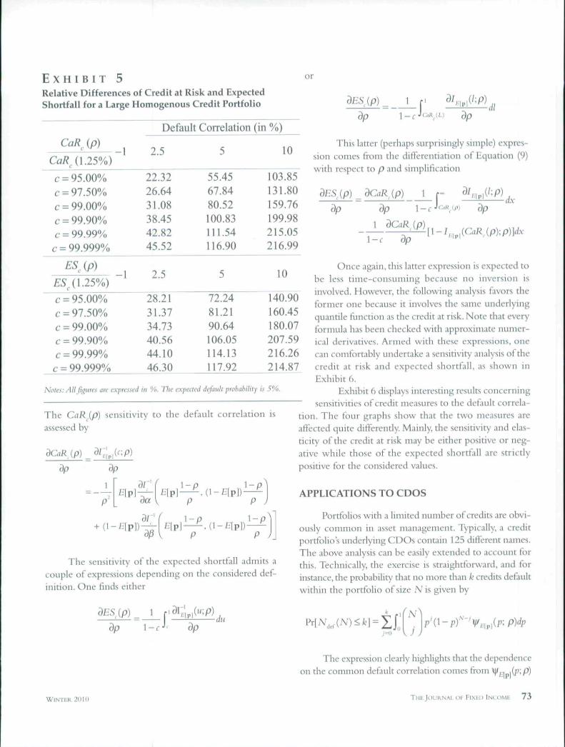
E X H I B I T 5Relative Differences of Credil at Risk and ExpectedShortfall for a Large Homogenous Credit Portfolio

or

Default Correlation (in

\.ip),(1.25%)

-1 2.5 10

c = 95,00%¿• = 97.50%c = 99.00%c = 99.90%C--99.99%c-99.999%

ES MES ^{\.25%)

c = 95.00%c- = 97.50%f = 99.00%c = 99.90%c = 99.99%

c = 99.999%

22.3226.6431.0838.4542.8245.52

2.5

28.2131.3734.7340.5644.1046.30

55.4567.8480.52100.83111.54116.90

5

72.2481.2190.64106.05114.13117.92

103.85131.80159.76199.98215.05216.99

10

140.90160.45180.07207.59216.26214.87

Motes: Allf[^nrei an- e.xpressed in %. The expected default probability is 5%.

The CaRip) sensitivity to the default correlation isassessed by

(p)

dp ¿L, •dt

This latter (perhaps surprisingly simple) expres-sion comes from the clitToreiitiation of Equation (9)with respect to p and simplification

{p)

dp

dGiR ip)

-r IP)dx

\-c dp

dp

da

a/-p

1 —

p

1 -

The sensitivity of the expected shortfall admits acouple of expressions depending on the considered def-inition. One finds either

Once again, this latter expression is expected tobe less time-consuming because no inversion isinvolved. However, the following analysis favors theformer one because it involves the same underlyingquantile function as the credit at risk. Note that everyformula has been checked with approximate numer-ical derivatives. Armed with these expressions, onecan comfortably undertake a sensitivity analysis of thecredit at risk and expected shortfall, as shown inExhibit 6.

Exhibit 6 displays interesting results concerning~ sensitivities of credit measures to the default correla-tion. The four graphs show that the two measures areafiected quite differently. Mainly, the sensitivity and elas-ticity of the credit at risk may be eitlier positive or neg-ative while those of the expected shortfall Are strictlypositive for the considered values.

APPLICATIONS TO CDOS

Portfolios with .1 limited number of credits are obvi-ously common in asset management. Typically, a creditportfolios underlying CDOs contain 125 different names.The above analysis can be easily extended to account forthis. Technically, the exercise is straightforward, and forinstance, the probabilit\- that no more than k credits detaultwithin the portfolio of size Nis given by

dp ¿r dpdu

The expression clearly higlilights that the dependenceon the common default correlation comes from V/iniÍPiP)

W i N I UK. 2(11(1 THE JOURNAL OF Fixnn INCOME 73

E X H I B I T 6

Sensitivities and Elasticities of Credit at Risk and the Expected Shortfall with Respect to the Common DefaultCorrelation

Elasticity

1U

3

2

1

1

\ 99%

Sensitivity

:

~~—-^,_ . .97.5% :

r^'->^.,^ '• 95"/.

c : ^ / . - - - • - - - - ' '

0,0 0.2 0.4 0,6 0,8

P

1.0

only. Additional siimilations could have nev-ertheless shown that distributions fora 125-name portfolio are very close to theirasymptotic counterpart. So, we favor asymp-totic distribution to investigate how holdersof the different tranches of a CDO areimpacted by a change in the default corre-lation. Holders of the so-called equity-tranche are exposed to the first defaults inthe portfolios while holders of the lasttranche are impacted only if the numberof defaults is significant. To fix this idea,let's consider the tranchnig of the Itraxxcontracts for which attachment points are0%. 3%, 6%, 9%, 12%. 22%. The associateddetachment points correspond to the upperlimit of the losses covered by the tranche.Exhibit 7 plots, for each considered tranche,the probability that losses will exceed thedetachment point versus the commondefault correlation p.

E X H I B I T 7

Probability That Losses Will Exceed the Detachment Point versus theCommon Default Correlation

0.2 0.4 0.6Common Default Correlation p

0.8 1.0

Note.^: dj, stands for detachment point and iorrcspontis to thf upper limit of the losses awercd by thetranche. Tlie plotted tail function is the probability that the loss exceeds the considered detachmentpoitit.

7 4 SFNsmvrry ANALYSIS OF CREDIT RISK MEASURES IN THE BETA BINOMUI FRAMEWORK WINTER 2010

Exhibit 7 exposes how holders of the differenttranches are differently impacted by the common defaultLorrekition. It ciin be observed first that holders of theequity tranche (whose detachmeiu point d is 3%) benefitfrom any increase of the common default correlation—acomplete loss being less probable. A reason for this is thatthe iinderlyinj^ references behave more identically as cor-relation increases; meaning that the common survival cor-relation increases too. Holders of the other tranches areclearly differently affected. Among them, investors in thesecond tranche remain rather exposed to the correlationrisk.

CONCLUSION

This article reconsiders the beta binomial approachfor modehng homogenous credit portfolios. It favors boththe expected default probabilit\' and the common defaultcorrelation to parameterize the inLxmg distribution. Thisarticle makes standard credit risk indicators flinctions ofthe correlation only and it sheds hghts on the model riskassociated with that parameter. Analytical expressions havebeen reported to allow seiLsitivity analysis. Simulationsconckide that default correlation is a key parameter toaccount for. Finally, it must be stressed that the idea exposedin the article is applicable to every mixing distribution tothe extent there exists a suitable function transformingstructural parameters into the expected default probabilityand the common default correlation.

A P P E N D I X A

PROPERTIES OF THE BETA DISTRIBUTION

This appendix displays some well-known properties ofthe beta distribution with respect to its shape parameters. Ifa- ß ~ y.then the hetj distribution is s^'nimctric with rcspectto f:'[pl = -7. Straitj;htforward Lomputatioiis give t '[pl= ;;>-;—and cor[X,,XJ = 7;^ = 4P'[pl. The standard deviation of the(nndom) default probability is bounded by 7. This limit cor-responds to / = (1 for which cor[X, X.] = 1. In such ;i case.eitlier all issuers survive or all default. The corresponding dis-tribution weights only 0 and 1. If instead, / = 1, the symmetricbeta distribution is the uniform one with I'|p] = -¡T ^nd

Analytical Expressions for Sensitivities

Due to the non-uniqueness of their representations,various expressions could be derived and reported for the deriv-atives of the cumulative density function of the beta distribu-tion and its associated inverse fiinction. Expressions below art-very appealing for programming on Mathematics—the package1 use throughout the article:

rc/0

- .v) - W{b) + \¡f{a + /.)!/,„,, (/>. a)

V{a)

and

X - J

where J3 (¡i, b) is the incomplete beta function defined by

ß,(i l , /') ^ in i"''(1 - 0 ' " ' < ' ' • 3F2 ( ' ' r '^2' 'h'- ''(• '':• ' ' r ' ^ ^ " '"" '^^~

ularized hypergcometric flmction and IjCis the digauuiia func-tion. The digamma function is the logarithm derivative of theEuler gamma function:

where

The Hinction F is a generalization to complex nunibcnof the factorial fimction since, for any integer n, V{n) = {n - I)!.,F., (dp 1Ï.,, ay i>,, /i.,, b^\ z) is defined by

WlNTKU 201(1 THEJOURNAL or Hixfi) INI_OME 7 5

with (ü),, = -pjTp is the Pochhammer's symbol. See Abramowitzand Stegun [1972] for more details on these functions.

ENDNOTES

I thank Areski Cousin and participants of the 2nd Inter-national Financial Risk Forum in Paris as well as seminar par-ticipants at Université de Nantes for comments. I acknowledgefinancial support from the IAE de Rennes (Graduate School ofBusiness Administration of the Université de Rennes 1) andCREM (the CNRS research unit number UMR 6211).

'A mixed logit-normal distribution is explicitly used inCreditPortfolioView (see Wilson [1997a,b]);a probit-normalone is used in Creditmetrics. Frey and McNeil |2002] havedemonstrated that the CreditRisk+ solution implicitly uses abeta mixing distribution for the default probability. As a result,the present article admits connections with the CreditRisk+framework, but this point is left for iliture research.

-The key point here is to develop an easy-to-understandway to manage credit portfolios within the beta binomial frame-work with no reference to the traditional (and rather obscure)shape parameters of the mixing distribution. This feature isdesirable because everybody involved in the credit industry isnot necessary "fluent" in statistics. Moreover, it is not so evi-dent that people involved in the credit business interpret beta'sshape parameters in the same way. It is welj known (see Freyand McNeil [2001]) that, when one of the two first momentsof the random default probability is fixed, the second momentor the default correlation determines the shape parameters ofthe beta mixing distribution. However, to our knowledge, noresearch has developed this way of reasoning further.

^Analytical expressions exposed in this article provide for-mulae to assess the impact of a correlation shift. This articletherefore admits some closed connections widi the recent streamof research dedicated to tlie introduction of non-constant defaultcorrelation in credit portfolios (see Burtschell, Gregory, andLaurent ]2ü(J7| for references). But this issue is left for futureresearch.

••Avoiding simulations, the approach is worthwhile forcredit analysts for at least a couple of reasons. First of all, it canspeed up computations and subsequent decisions making.Second, It prevents drawbacks of rival simulation-based methods.It is well knowu that the estimates they pmvide can be fairlyunstable, as they depend on the number of simulation runs andon the way the random figures are generated. These methodscan even fail to provide safe results. Credit risk measures areindeed intimately related to the tail of the distribution, whichis challenging to capture by simulation.

that, except speculators, very few investors wouldinvest in credit portfolios with a such a significant expecteddefault probability.

'To see this, it is sutEcieiit to note that the conditional vari-ante of the proportion g"!'' ' ."" | p] = ''' P' tends to 0.

The latter appears less time-consuming than the formerbecause no inversion is required. This remark may be hclptul,tor who wants to make intensive computations.

REFERENCES

Abramowitz, M., and I. Stegun. Handbook of MathematicalFunctions. Hover, 1972.

Artzner, Ph., F. DelbaenJ.-M. Eber, and D. Heath. "CoherentMeasures of Risk." Mathenuuical Findtur, Vol. '). No. 3 (I9^>9),pp, 203-228.

Burtschell, X..J. Gregory, and J.P Laurent. "Beyond the GaussianCopula: Stochasnc and Local C:ornrlation."_/t'Mríífj/ of Credit Risk,Vol. 3, No. 1 (2007).pp.31-f)2.

Frey, R., and A. McNeil. "Modelhng Dependent Defaults."Working Paper, ETH Zürich, 2001.

/'VaR and Expected Sliortfall m Portfolios of DependentCredit Risks: Conceptual and Practical Insights."_/iKiriiiï/ ofBanking & Finance, Vol. 26, No. 7 (2002), pp. 1317-1334.

. "Dependent Defaults in Models of Portfolio Credit Risk.">i(riM/()/"Ri.tfe,Vol.6,No. 1 (2003), pp. 59-92.

Renault, Ü., and A. de Servigny. Measuring and Managing CreditRisk (The Standard and Poors Guide). McGraw-Hill, 2004.

Schönbucher, P. "Taken to the Limit: Simple .ind Not-So-Simple Loan-Loss Distributions." H^ILMOTT Magazine,2 (2003), pp. 63-73.

Wilson, T. "Portfolio Credit Risk Ir Risk, 10 (September 19y7a).pp. 111-117.

. "Portfolio Credit Risk 11." Risk, 10 (October 1997b).pp. 56-61,

To order reprints of this article, please contact Dewey Ihlniieri atdptitniieri@iijournah.com or 212-224-3675.

7 6 SENsiTivtrv ANAIYSIS OF CREDIT RISK MEASURES IN TIIE BETA BINOMIAL FRAMEWORK WlNfLK 2IMII

©Euromoney Institutional Investor PLC. This material must be used for the customer's internal business use

only and a maximum of ten (10) hard copy print-outs may be made. No further copying or transmission of this

material is allowed without the express permission of Euromoney Institutional Investor PLC. Source: Journal of

Fixed Income and http://www.iijournals.com/JFI/Default.asp