sensitivity analysis of statistical measures for the ... · technische mechanik, 30, 4, (2010),...

TECHNISCHE MECHANIK,30, 4, (2010), 297– 315

submitted: October 31, 2009

Sensitivity analysis of statistical measures for the reconstruction ofmicrostructures based on the minimization of generalized least-squarefunctionals

D. Balzani, D. Brands, J. Schroder, C. Carstensen

For the simulation of micro-heterogeneous materials the FE2-method provides incorporation of the mechanicalbehavior at the microscale in a direct manner by taking into account a microscopic boundary value problem basedon a representative volume element (RVE). A main problem of this approach is the high computational cost, whenwe have to deal with RVEs that are characterized by a complex geometry of the individual constituents. This leadsto a large number of degrees of freedom and history variablesat the microscale which needs a large amount ofmemory, not to mention the high computation time. Therefore, methods that reduce the complexity of such RVEsplay an important role for efficient direct micro-macro transition procedures. In this contribution we focus on ran-dom matrix-inclusion microstructures and analyze severalstatistical measures with respect to their influence onthe characterization of the inclusion phase morphology. For this purpose we apply the method proposed in Balzaniand Schroder (2008); Balzani et al. (2009a), where an objective function is minimized which takes into accountdifferences between statistical measures computed for theoriginal binary image of a given real microstructure anda simplified statistically similar representative volume element (SSRVE). The analysis with respect to the capabilityof the resulting SSRVEs to reflect the mechanical response insome simple independent virtual experiments allowsfor an estimation of the importance of the investigated statistical measures.

1 Introduction

Many fields in metal processing like bending, deep-drawing or hydro-forming require a high ductility and stiffnessof the used steel. According to advanced requirements in high-tech applications minimization of the dead weightby simultaneously increasing safety demands is one of the major goals in industry. In this context multi-phasesteels have the potential to fulfill these requirements. This is due to the fact that the interplay between the individ-ual constituents on the microscale yield outstanding strength and ductility properties. However, the complicatedinteractions of the individual phases of the micro-heterogeneous composite lead to complex local and global hard-ening effects and failures on the microscale. In order to capture these phenomena up to a certain accuracy wefocus on a two-scale modeling approach. In this framework weattach a sufficient large section of the microstruc-ture, approximated by a representative volume element (RVE), to each point of the macroscale. The numericaltreatment of this approach is known as the direct micro-macro-transition procedure or the FE2-method, see e.g.Smit et al. (1998), Brekelmans et al. (1998), Miehe et al. (1999), Schroder (2000), and Geers et al. (2003). Ba-sic ideas for the direct micro-macro-transition approach with the application to dual-phase steels (DP-steels) aregiven in Schroder et al. (2008). The drawback of this approach is the high computational cost (high computationtimes), when we deal with large random microstructures. Furthermore, a large number of history variables occursin this case which needs a large amount of memory. In order to circumvent these drawbacks we focus on theconstruction of statistically similar representative volume elements (SSRVEs) which are characterized by a muchless pronounced complexity than the real random microstructures. The basic idea for this procedure is to find asimplified SSRVE, whose selected statistical measures are as close as possible to the real microstructure. The un-derlying minimization procedure is governed by least-square functionals, which compare the statistical measuresof the real microstructure with the ones of the SSRVE. Besidethe volume fraction we can usen-point probabiltyfunctions, lineal-path functions, values of the specific internal surface and integral of mean curvature, etc. Parzen(1992) has shown that the two-point probability density function is correlated to the power spectral density in thefrequency domain. Based on this work Povirk (1995) computeda simplified RVE for a composite consisting ofa matrix with circular inclusions. In this generalized approach we describe the inclusion phase with splines andcompare different statistical measures, in this context see Balzani and Schroder (2008); Balzani et al. (2009b).

297

2 Mechanical framework

In this work we focus on a direct micro-macro transition approach which takes into account a micromechani-cal boundary value problem for the determination of material properties at the macroscale. At the microscalean isotropic finiteJ2-plasticity model with a von Mises yield law is taken into account for the response of theindividual phases building up the microstructure.

2.1 Kinematics at different scales

Let B ⊂ R3 denote a physical body at the microscale in its undeformed (reference) configuration at timet = t0,

parameterized in position vectorsX, whereinR3 is the euclidian three-dimensional space. A deformed (actual)

configuration is denoted byS ⊂ R3, parameterized byx at a fixed timet ∈ R+. Concentrating on the Boltzman

continuum theory the deformation of the body can be interpreted as the motion of material points. The non-linear, continuous and one-to-one transformationϕ(X, t) : B → S maps at timet ∈ R+ pointsX ∈ B of themicroscopic reference configuration onto pointsx ∈ S of the actual microscopic configuration. For the descriptionof deformations we define the microscopic deformation gradient

F(X) := Grad[ϕt(X)] . (1)

At the macroscale we use the analogous definitions and use overlined characters to identify macroscopic quantities,then we consider the transformation mapϕ(X, t) : B → S with the macroscopic physical bodiesB andS in thereference and in the actual configuration, respectively. Then, the macroscopic deformation gradient is defined by

F(X) := Grad[ϕt(X)] . (2)

2.2 Constitutive modeling of the individual phases on the microscale

In order to solve the boundary value problem on the microscale, we have to set up constitutive equations forthe individual phases on the microscale. During the deformation process the composite exhibits large plasticdeformations. Due to the lack of experiments, we apply an isotropic material behavior for both phases, the metallicmatrix and the metallic inclusion. It seems to be reasonableto use an isotropic finite elastoplasticity formulationbased on the multiplicative decomposition of the deformation gradientF = F

eF

p in elasticFe and plasticFp

parts, see Kroner (1960), Lee (1969). For details of the thermodynamicalformulation as well as for the numericaltreatment we refer to Simo (1988, 1992), Simo and Miehe (1992), Peric et al. (1992), Miehe and Stein (1992), andMiehe (1993). In the following we give a brief summary of the used framework. The basic kinematical quantitiesare

b = FFT = F

eb

p (Fe)T , bp = F

p (Fp)T , and be = F

e (Fe)T , (3)

with the spectral decomposition of the elastic finger tensor

be =

3∑

A=1

(λeA)2nA ⊗ nA , (4)

wherenA denotes the eigenvectors andλeA the eigenvalues ofbe. The stored energy function is assumed to be of

the formψ = ψe(be) + ψp(α), whereinα denotes the equivalent plastic strains. Following Simo (1992) we use aquadratic free energy function

ψe =λ

2[ǫe1 + ǫe2 + ǫe3]

2 + µ[(ǫe1)2 + (ǫe2)

2 + (ǫe3)2] (5)

in terms of the logarithmic elastic strainsǫeA = log(λeA); λ andµ are the Lame constants. In order to model an

exponential-type hardening of the individual phases we apply the well-known function

ψp = y∞α−1

η(y0 − y∞) exp(−ηα) +

1

2h α2 . (6)

298

However, the conjugated stress-like variable, defined asβ := ∂αψp , is

β = y∞ + (y0 − y∞) exp(−ηα) + h α . (7)

Herein,y0 is the initial yield strength,y∞ andη describe an exponential hardening behavior andh is the slope ofa superimposed linear hardening. The yield criterium is given by

φ = ||devτ || −

√2

3β ≤ 0 with τ =

3∑

A=1

τA nA ⊗ nA and τA =∂ψe

∂ǫe. (8)

Herein, the Kirchhoff stresses are denoted byτ . The flow rule for the plastic quantity is integrated using animplicitexponential update algorithm, which preserves plastic incompressibility (Weber and Anand (1990), Simo (1992),and Miehe and Stein (1992)). The first Piola-Kirchhoff stresses on the microscale are computed byP = τ F

−T .For the numerical implementation we follow the algorithmicformulation in a material setting as proposed inKlinkel (2000).

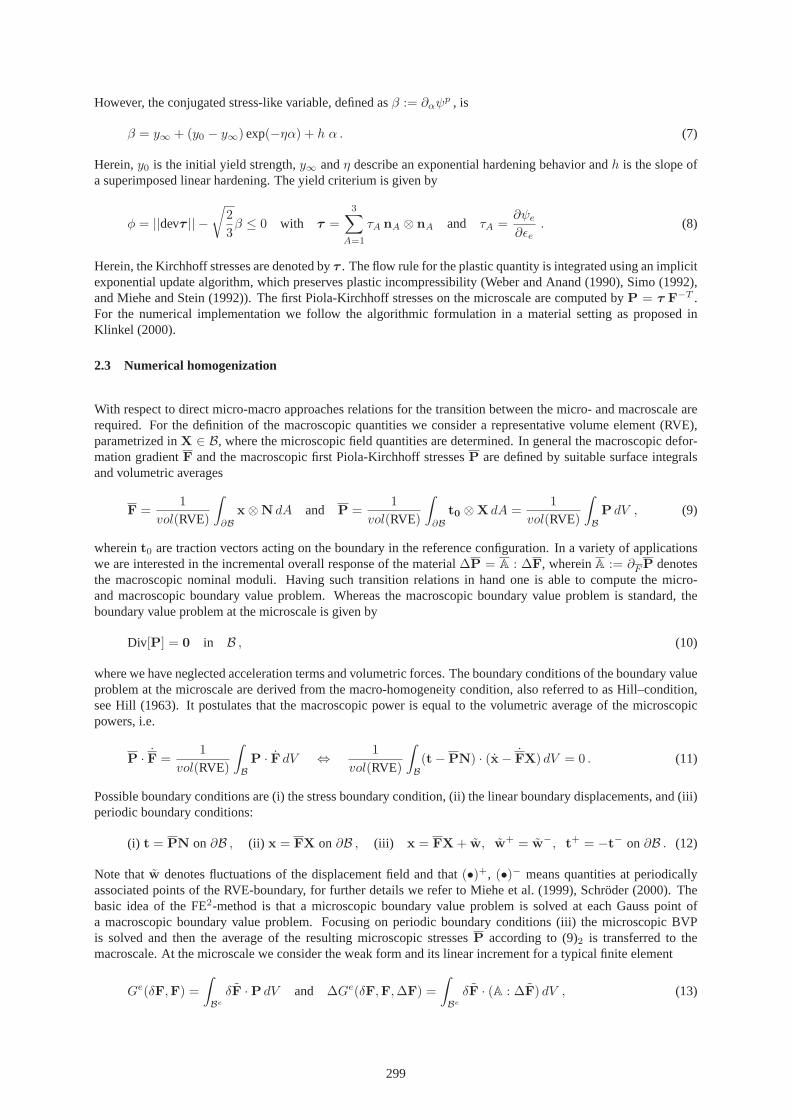
2.3 Numerical homogenization

With respect to direct micro-macro approaches relations for the transition between the micro- and macroscale arerequired. For the definition of the macroscopic quantities we consider a representative volume element (RVE),parametrized inX ∈ B, where the microscopic field quantities are determined. In general the macroscopic defor-mation gradientF and the macroscopic first Piola-Kirchhoff stressesP are defined by suitable surface integralsand volumetric averages

F =1

vol(RVE)

∫

∂B

x ⊗ N dA and P =1

vol(RVE)

∫

∂B

t0 ⊗ X dA =1

vol(RVE)

∫

B

P dV , (9)

whereint0 are traction vectors acting on the boundary in the referenceconfiguration. In a variety of applicationswe are interested in the incremental overall response of thematerial∆P = A : ∆F, whereinA := ∂F P denotesthe macroscopic nominal moduli. Having such transition relations in hand one is able to compute the micro-and macroscopic boundary value problem. Whereas the macroscopic boundary value problem is standard, theboundary value problem at the microscale is given by

Div[P] = 0 in B , (10)

where we have neglected acceleration terms and volumetric forces. The boundary conditions of the boundary valueproblem at the microscale are derived from the macro-homogeneity condition, also referred to as Hill–condition,see Hill (1963). It postulates that the macroscopic power isequal to the volumetric average of the microscopicpowers, i.e.

P · F =1

vol(RVE)

∫

B

P · F dV ⇔1

vol(RVE)

∫

B

(t − PN) · (x − FX) dV = 0 . (11)

Possible boundary conditions are (i) the stress boundary condition, (ii) the linear boundary displacements, and (iii)periodic boundary conditions:

(i) t = PN on ∂B , (ii) x = FX on ∂B , (iii) x = FX + w, w+ = w

−, t+ = −t

− on ∂B . (12)

Note thatw denotes fluctuations of the displacement field and that(•)+, (•)− means quantities at periodicallyassociated points of the RVE-boundary, for further detailswe refer to Miehe et al. (1999), Schroder (2000). Thebasic idea of the FE2-method is that a microscopic boundary value problem is solved at each Gauss point ofa macroscopic boundary value problem. Focusing on periodicboundary conditions (iii) the microscopic BVPis solved and then the average of the resulting microscopic stressesP according to (9)2 is transferred to themacroscale. At the microscale we consider the weak form and its linear increment for a typical finite element

Ge(δF,F) =

∫

Be

δF · P dV and ∆Ge(δF,F,∆F) =

∫

Be

δF · (A : ∆F) dV , (13)

299

with the microscopic nominal moduliA := ∂F P. The fluctuation parts of the actual, virtual and incrementaldeformation gradient can be approximated by using standardansatz functions for the fluctuation displacementsinterpolating between the fluctuation parts of displacements d, virtual displacementsδd, and incremental dis-placements∆d. Then we obtain the discrete representation of the linearized problem

δDT {K∆D + R} = 0 , (14)

with the global vectors of incremental fluctuation displacementsD and residual forcesR, and with the globalmicroscopic stiffness matrixK. In each iteration the actual increments of displacement fluctuations are computedfrom (14) and updated, i.e.D ⇐ D + ∆D, until |R| < tol, wheretol represents the algorithmic tolerance. At themacroscale a standard FE-discretization is considered where the macroscopic moduli which enter the macroscopicstiffness matrix, are computed by

A = 〈A〉 −1

vol(RVE)L

TK

−1L with 〈A〉 =

1

vol(RVE)

∫

B

A dV , (15)

denoting the classical Voigt bound. Herein, the second additive term represents a softening modulus necessary forthe consistent linearization. For its calculation the matrix

L =nele

Ae = 1

∫

Be

BT

A dV (16)

makes use of the same assembling operator applied for assembling the global microscopic stiffness matrix;Bdenotes the standard B-matrix. For details on deriving the consistent macroscopic moduli please see e.g. Mieheet al. (1999); Schroder (2000).

3 Method for the construction of SSRVEs

The method for the generation of statistically similar representative volume elements (SSRVEs) is substantiated onthe approach for the construction of periodic structures proposed in Povirk (1995). There, the position of circularinclusions with constant and equal diameters is optimized by the minimization of a least-square functional takinginto account the side condition that the spectral density ofthe periodic RVE should be as similar as possible to theone of the non-periodic microstructure. For our further studies we consider the generalized minimization problem

L(γ) → min with L(γ) =

nsm∑

L=1

ω(L)L(L)SM (γ) , (17)

which has been introduced in Balzani et al. (2009a), see alsoBalzani et al. (2009b).L(L)SM describes the least-square

functional defined by a suitable difference of a particular statistical measure computed for the real microstructureand for the SSRVE. The number of considered statistical measures is represented bynsm, whereas the weightingfactorω(L) levels the influence of the individual measures with number(L). For the description of a general inclu-sion phase morphology in the SSRVE we assume a suitable two-dimensional parameterization controlled by thevectorγ. In our analysis we focus on splines for the parameterization, thus, the coordinates of the sampling pointsenterγ.For an illustration of the main characteristics of the minimization problem a simple test example is given in Balzaniet al. (2009a), where the spectral density is taken into account as the main statistical measure. There an assumedreal two-dimensional microstructure with one inclusion isconsidered as a target structure, which is generated byrandomly distributing four sampling points. Then a SSRVE isconstructed by one spline with four sampling pointsas well, where three sampling points are set to the values used for the generation of the target structure. Hence, weend up in a problem where only one sampling point is free to move in the optimization process and one is able tovisually analyze the objective function plotted over the degrees of freedom. As shown in Balzani et al. (2009a) theresulting objective function is far away from being smooth.Apparently, the computation of the discrete spectraldensity and the volume fraction takes into account a specificdiscrete image resolution. Hence, this leads to anon-smooth function and precludes the application of standard gradient-based optimization procedures. This is arather structural problem since most statistical measuresare based on a discrete image characterized by a givenresolution. In addition to this, the problem is non-convex and thus, we have to deal with many local minima whenincreasing the number of degrees of freedom.To overcome the difficulties arising from the particular minimization problem a moving frame algorithm is applied.

300

For this purpose random initial sampling point coordinatesx0,k, y0,k are generated first, which direct to the sam-pling pointM0,k. Then furthernmov random pointsMj,k(xj,k, yj,k), j = 1..nmov in a frame of the size2a× 2aare generated, see Fig. 1a, and the objective function is evaluated for each generated sampling point.

M4

M2

M1

M3

M4

M2

M1

M3

Framek

a

a

M0 ⇐ M1

L(M0,k) :M1

framek + 1

new randomMj

for j = 1...4:

L(M0,k+1)

if L(Mj,k+1) >if L(M1,k) <

framek + 2 b= framek + 1

M0

M0

M0d

a) b) c)

Figure 1: Schematic illustration of moving frame algorithm.

Then the initial sampling point moves to the sampling pointM0,k+1 defined by the lowest value ofL and theiteration counter is initializedliter = 0, see Fig. 1b . If the frame center remains unaltered, i.e. no lower valueof L is found in this iteration step (M0,k+1 = M0,k+2), we setliter = liter + 1, see Fig. 1c. Ifliter = litermax

the stopping criterion is reached and the actual minimal value ofL is interpreted as local minimum associated tothe starting value. In addition, this procedure is repeateda predefined number of cycles with different randomstarting values. If a high fraction of minimizers of the individual optimization cycles leads to similar samplingpoint coordinates, then we choose this result as an appropriate solution. In order to improve the method the framesizea can be modified depending on the difference|d| andliter. Furthermore, a combination with a line-searchalgorithm is implemented, whereL is also evaluated at a number ofnline points interconnecting the frame centerpointM0 with the random pointsM1,M2, . . .Mnmov

.The moving-frame algorithm used here is rather a statistical method for finding the minima. Further possiblitiesfor the solution of non-smooth optimization problems can befound in e.g. Kolda et al. (2003), Conn et al. (2009)and Makela and Neittaanmaki (1992). A possible improvement of the minimization algorithm may be obtainedby filtering out structural oscillations associated to the non-smoothness in order to obtain at least locally smoothobjective function approximations. In this case bundle methods where generalized gradient information is exploited(e.g. Schramm and Zowe (1992)) could be used or the Nelder-Mead method (Nelder and Mead (1965)), if onlyfunction evaluations are desireable.

4 Numerical sensitivity analysis of different statisticalmeasures

In this section we study the significance of different statistical measures for the description of the inclusion mor-phology with respect to the mechanical behavior. Therefore, we compare the mechanical response of a randomlygenerated microstructure, dealing as a target structure, with the response of different types of SSRVEs. The targetstructure is obtained by applying the Boolean method, whereellipsoids built from the matrix material are insertedat random points in a pure inclusion material until a predefined volume fraction is reached. For this contributionwe consider the target structure shown in Fig. 2a, which is the result of applying the Boolean method for an aspectratio of the semi-principal axis ofrx/ry = 14.3 and randomly generatedrx ∈ [3, 6].

a) b) c)rx/ry = 14.3, rx ∈ [3, 6] PV = 0.1872 nele = 5452 , ndof = 21930

Figure 2: Steps for the generation of the target structure: a) result of the Boolean method, b) smoothed targetstructure, and c) discretization of the target structure.

301

The stopping criterion for the Boolean method is given by a volume fraction of the inclusion phase of0.2 ± 1%.In the next step we smoothen the boundaries of the inclusionsin order to avoid singularities, see Fig. 2b, thenthe resulting volume fraction isPV = 0.1872. For Finite-Element simulations the smoothened target structure isdiscretized by5452 triangular elements with quadratic shape functions, see Fig. 2c. For our analysis we considerthree different types of virtual macroscopic experiments:i) horizontal uniaxial tension, ii) vertical uniaxial tensionand iii) simple shear, cf. Fig. 3.

σx

σyux ux

0

250

500

750

1000

1250

1500

1750

2000

2250

2500

0 0.01 0.02 0.03 0.04 0.05 0.06 0.07 0.08

σx

[MP

a]

△lx/lx,0

Horizontal tension

ferritemartensite

0

250

500

750

1000

1250

1500

1750

2000

2250

2500

0 0.01 0.02 0.03 0.04 0.05 0.06 0.07 0.08

σy

[MP

a]

△ly/ly,0

Vertical tension

ferritemartensite

0

250

500

750

1000

1250

1500

0 0.01 0.02 0.03 0.04 0.05 0.06 0.07 0.08

σxy

[MP

a]△ux/ly,0

Simple shear

ferritemartensite

Figure 3: Virtual macroscopic experiments of the pure matrix (ferrite) and inclusion material (martensite); at themicroscale periodic boundary conditions are used.

At the microscale the periodic boundary conditions (iii) are used, cf. (12). For the ferritic matrix material and themartensitic inclusions the material parameters given in Table 1 are used. Then a stress-strain response as shown inFig. 3 is observed for the individual phases in the three virtual experiments.

phase λ µ y0 y∞ η h[MPa] [MPa] [MPa] [MPa] [-] [-]

ferrite 118,846.2 79,230.77 260.0 580.0 9.0 70.0martensite 118,846.2 79,230.77 1000.0 2750.0 35.0 10.0

Table 1: Material parameters of the single phases

The SSRVEs are constructed considering several combinations of statistical measures as optimization criteria.Since the volume fraction is an important overall information with view to the influence of the morphology on themechanical properties we take it into account for all SSRVE constructions given in this contribution. Then, theassociated least-square functional reads

L(1) := LV (γ) =

(1 −

PSSRV EV (γ)

PrealV

)2

, (18)

which is used within the general minimization problem (17).Since we analyze two-dimensional images the volumefractionsPreal

V andPSSRV EV required for the computation ofLV are computed by

PV :=VI

V, (19)

whereVI denotes the area of the inclusion phase andV the total area of the considered microstructure image. Thecomputation of the volume fraction is performed directly from the binary images of the given target structure andthe SSRVE.

302

4.1 Sensitivity for two different statistical measures

In a first step we study the significance of several statistical measures for the generation of SSRVEs with respect totheir mechanical behavior compared with the target structure. As already mentioned the volume fraction is in allcases an additional constraint in the optimization process.

4.1.1 Specific internal surface

In Ohser and Mucklich (2000) the specific internal surface is mentioned asone basic parameter to describe mi-crostructure morphology. It seems to be a suitable measure for the specification of the inclusion phase’s distribu-tion. In the general three-dimensional case this parameteris given by

P3DS :=

SI

V, (20)

with the interface areaSI separating the inclusion from the matrix material and the total volumeV of the consideredmicrostructure. Here we focus on the two-dimensional case and so this parameter can be calculated by

PS :=4

πLA , (21)

whereinLA is the specific boundary line length between the two phases. It is mentioned that Eq. (21) can bederived from Crofton’s slice formulas for compact bodies, see Ohser and Mucklich (2000). Then the associatedleast-square functional reads

L(2) := LS(γ) =

(1 −

PSSRV ES (γ)

PrealS

)2

, (22)

and together with the volume fraction functional (18) we getthe first minimization problem

L1(γ) =

2∑

L=1

ω(L)L(L) = ωV LV (γ) + ωSLS(γ) → min with ωV = ωS = 1 , (23)

For the parameterization of the inclusion morphology of theSSRVE splines are used, thus, the coordinates ofthe sampling points arranged inγ represent the degree of freedom in the optimization problem. Here we takeinto account four types of inclusion parameterization: oneinclusion with three sampling points (type I) leadingto convex inclusions, one inclusion with four sampling points (type II), and two inclusions with three and foursampling points each (type III and type IV), respectively. The results of the optimization process considering themicrostructure in Fig. 2 as target are shown in Fig. 4. The decreasing values of the objective function togetherwith an increasing number of sampling points can be observed. This is an expected behavior as we know thatthe number of sampling points reflects the degree of freedom for the generation, thus also the complexity of theinclusions. But the higher complexity implicates a larger quantity of finite elements in the discretization. This isa non-negligible aspect in the context of replacing a RVE with an arbitrary complex inclusion morphology by asimpler one with similar mechanical behavior.

Type I:ndof = 2394 Type II: ndof = 2762 Type III: ndof = 4058 Type IV: ndof = 4650

L1 = 0.0188 L1 = 1.5 · 10−9L1 = 1.5 · 10−9

L1 = 2.4 · 10−10

Figure 4: Discretization of the SSRVEs resulting from the minimization ofL1.

303

In order to study the SSRVEs capability to reflect the mechanical response of the target structure we compare thestress-strain response of the SSRVEs with the response of the target structure in the three virtual experiments, seeFig 3. The resulting stress-strain curves are shown in Fig. 5. For the estimation of the accuracy we compute therelative errors

r(i)x =σreal

x,i − σSSRV Ex,i

σrealx,i

, r(i)y =σreal

y,i − σSSRV Ey,i

σrealy,i

, r(i)xy =σreal

xy,i − σSSRV Exy,i

σrealxy,i

, (24)

as the deviation of the SSRVE stress response from the targetstructure response at each evaluation pointi. Toconsider relative quantities is important here in order to be able to compare the different virtual experiments. Thenthe average error for each virtual experiment is computed by

r =

√√√√ 1

n

n∑

i=1

[r(i)( i

n△lmax/l0)

]. (25)

As a comparative measure we define the overall average error

r∅ =1

3(rx + ry + rxy) . (26)

The error values for the experiments based on the SSRVEs generated throughL1 are shown in Table 2.

Stress-Strain Response Relative Mechanical Error

250

300

350

400

450

500

550

0 0.01 0.02 0.03 0.04 0.05 0.06 0.07 0.08

σx

[MP

a]

△lx/lx,0

Horizontal tension

targetI

IIIIIIV

0

0.05

0.1

0.15

0.2

0 0.01 0.02 0.03 0.04 0.05 0.06 0.07 0.08

r x

△lx/lx,0

Horizontal tensionI

IIIIIIV

250

300

350

400

450

500

550

0 0.01 0.02 0.03 0.04 0.05 0.06 0.07 0.08

σy

[MP

a]

△ly/ly,0

Vertical tension

targetI

IIIIIIV

0

0.05

0.1

0.15

0.2

0 0.01 0.02 0.03 0.04 0.05 0.06 0.07 0.08

r y

△ly/ly,0

Vertical tensionI

IIIIIIV

100

125

150

175

200

225

250

275

0 0.01 0.02 0.03 0.04 0.05 0.06 0.07 0.08

σxy

[MP

a]

△ux/ly,0

Simple shear

targetI

IIIIIIV

0

0.05

0.1

0.15

0.2

0 0.01 0.02 0.03 0.04 0.05 0.06 0.07 0.08

r xy

△ux/ly,0

Simple shearI

IIIIIIV

Figure 5: Results of the virtual experiments using the discretizations of the SSRVEs based onL1 (Figure 4).

304

In Fig. 5 the stress-strain curves of each SSRVEs shows different accuracies with respect to the virtual experiments.In the first test, the horizontal tension, the mechanical errors decrease depending on the complexity of the SSRVE,but also type IV has an error above five percent at most evaluation points. On the other hand in the vertical tensionthe behavior differs totally. Here the types I and II show a good agreement with the results of the target structure(ry < 1%) and the both other types differ more. But all errors are lower compared to them from the horizontaltension. The simple shear experiments show qualitatively similar results as we have seen in the horizontal tensiontest. But the error values particularly the higher order types are at a lower level, see also Table 2. If we take alook at the overall average error in Table 2 we see that the specific internal surface and sufficient complexity ofthe SSRVEs inclusions yield slightly the mechanical response of the target structure. But the significant differentaccuracies comparing the both tension experiments show that the specific internal surface does not contain enoughdirectional information of the inclusion morphology and istherefore not able to cover macroscopic anisotropyinformation. Thus, we have to take another statistical measure into account to describe this characteristic of amicrostructure.

SSRVE L1 LV LS nele erx ery erxy er∅

type [-] [-] [-] [-] [%] [%] [%] [%]

I 0.0188 0.0 0.0188 566 12.44± 2.83 0.39± 0.40 9.18± 3.18 7.34II 1.5·10−9 0.0 1.5·10−9 658 9.67± 2.18 0.27± 0.16 2.23± 1.09 4.06III 1.5·10−9 0.0 1.5·10−9 982 9.12± 2.09 4.68± 1.35 2.16± 1.12 5.32IV 2.4·10−10 0.0 2.4·10−10 1130 6.52± 1.43 3.00± 0.85 0.66± 0.17 3.40

Table 2: Values of the objective functionL1 and the errorsr using the SSRVEs shown in Figure 4.

4.1.2 Specific integral of mean curvature

As an other basic parameter for the descrictpion of the morphology of heterogeneous microstructures the specificintegral of mean curvature for the general three-dimensional case is defined as

P3DM :=

1

2V

∫

S

(min

β[κ] + max

β[κ]

)ds , (27)

cf. Ohser and Mucklich (2000). The integral is evaluated over the interface S between the inclusion and matrixphase of the average curvatureκ := κ(β) varying with directionβ in the tangential plane. For the two-dimensionalcase the specific integral of mean curvature can be calculated by

PM := 2πXA , (28)

with the specific Euler number following Ohser and Mucklich (2000). For the optimization process we formulatethe associated least-square functional

L(2) := LM (γ) =

(1 −

PSSRV EM (γ)

PrealM

)2

, (29)


L2 = 0.2648 L2 = 8.5 · 10−4L2 = 8.5 · 10−4

L2 = 8.5 · 10−4


305

As before we also consider the functional (18) and get the second minimization problem

L2(γ) =

2∑

L=1

ω(L)L(L) = ωV LV (γ) + ωMLM (γ) → min with ωV = ωM = 1 . (30)

The vectorγ contains the sampling points for the generation of SSRVEs bysplines. We again consider fourdifferent types of inclusion parametrization, for detailssee Section 4.1.1. As the result from the optimization weget the four SSRVEs shown in Fig. 6.

Stress-Strain Response Mechanical Error

250

300

350

400

450

500

550

0 0.01 0.02 0.03 0.04 0.05 0.06 0.07 0.08

σx

[MP

a]

△lx/lx,0

Horizontal tension

targetI

IIIIIIV

0

0.05

0.1

0.15

0.2

0 0.01 0.02 0.03 0.04 0.05 0.06 0.07 0.08r x

△lx/lx,0

Horizontal tensionI

IIIIIIV

250

300

350

400

450

500

550

0 0.01 0.02 0.03 0.04 0.05 0.06 0.07 0.08

σy

[MP

a]

△ly/ly,0

Vertical tension

targetI

IIIIIIV

0

0.05

0.1

0.15

0.2

0 0.01 0.02 0.03 0.04 0.05 0.06 0.07 0.08

r y

△ly/ly,0

Vertical tensionI

IIIIIIV

100

125

150

175

200

225

250

275

0 0.01 0.02 0.03 0.04 0.05 0.06 0.07 0.08

σxy

[MP

a]

△ux/ly,0

Simple shear

targetI

IIIIIIV

0

0.05

0.1

0.15

0.2

0 0.01 0.02 0.03 0.04 0.05 0.06 0.07 0.08

r xy

△ux/ly,0

Simple shearI

IIIIIIV

Figure 7: Results of the virtual experiments using the discretizations based onL2 (Figure 6).

The stress-strain curves of the three virtual experiments (Fig. 3) performed with the discretized SSRVEs fromFig. 6 are shown in Fig. 7 compared to the results of the targetstrcuture. For the comparision of these results wecompute again the errors (24)-(26), which are listed in Table 3.

SSRVE L2 LV LM nele erx ery erxy er∅

type [-] [-] [-] [-] [%] [%] [%] [%]

I 0.2648 0.0 0.2648 560 11.58± 2.66 0.33± 0.20 2.40± 0.65 4.77II 8.5·10−4 0.0 8.5·10−4 628 9.02± 2.00 0.58± 0.31 0.85± 0.18 3.48III 8.5·10−4 0.0 8.5·10−4 762 9.79± 2.21 2.65± 0.57 0.84± 0.19 4.43IV 8.5·10−4 0.0 8.5·10−4 1598 10.20± 2.32 1.22± 0.54 1.99± 0.90 4.47


In Fig. 7 the stress-strain curves for the vertical tension and the simple shear tests of the SSRVEs show goodagreements with the results of the target structure. In bothcases the error is lower than5% in all evaluation points.But in the first test, the horizontal tension, all types of SSRVE have errors above10% in several evaluation points.

306

The errors in Table 3 confirm the observation from the stress-strain curves and also shows that an increasing numberof sampling points does not achieve better results. The errors of the horizontal and the vertical tests differ againin a strong manner and so the specific integral of mean curvature is again not a parameter covering directionalinformation of the microstructure. Also a larger range in the values of the overall average errors can be observedin Table 2, which are associated to the volume fraction and the specific internal surface, compared to the results inthis section here.

4.1.3 Spectral density

The results from Section 4.1.1 and 4.1.2 show that we need to consider statistical measures which cover directionalinformation. A possibility is the (discrete) spectral density (SD) for the inclusion phase of a binary image, whichis computed by the multiplication of the (discrete) Fouriertransform with its conjugate complex. The discrete SDis defined by

PSD(m, k) :=1

2πNxNy

|F(m, k)|2 (31)

with the Fourirer transform given by

FI(m, k) =

Nx∑

p=1

Ny∑

q=1

exp

(2 i π mp

Nx

)exp

(2 i π k q

Ny

)χI(p, q) . (32)

The maximal numbers of pixels in the considered binary imageare given byNx andNy; the indicator function isdefined as

χ :=

{1, if (p, q) is in inclusion phase0, else.

(33)

For the consideration of the SD in the optimization problem we write the least-square functional

L(2) := LSD(γ) =1

NxNy

Nx∑

m=1

Ny∑

k=1

(Preal

SD (m, k) − PSSRV ESD (m, k,γ)

)2, (34)

and together with (18) we get the minimization problem

L3(γ) =

2∑

L=1

ω(L)L(L) = ωV LV (γ) + ωSDLSD(γ) → min with ωV = ωSD = 1 . (35)

The evaluation of the functional (34) requires a more detailed treatment since the others are scalar-valued. In orderto get reasonable results and to obtain an efficient optimization procedure it may be necessary not to consider thespectral density at a very fine resolution level (Nx andNy very large). Therefore, first the SD is computed at ahigh resolution. Second, the spectral density is rebinned such that a lower resolution is obtained, which means thatNx andNy are decreased. Finally, the SD is normalized by dividing by its maximum value maxm,k[PSD(m, k)].In Fig. 8 the resulting SSRVEs from the optimization processare shown, whereas the same types of SSRVE


L3 = 0.0144 L3 = 0.0133 L3 = 0.0127 L3 = 0.0100


307


250

300

350

400

450

500

550

0 0.01 0.02 0.03 0.04 0.05 0.06 0.07 0.08

σx

[MP

a]

△lx/lx,0

Horizontal tension

targetI

IIIIIIV

0

0.05

0.1

0.15

0.2

0 0.01 0.02 0.03 0.04 0.05 0.06 0.07 0.08

r x

△lx/lx,0

Horizontal tensionI

IIIIIIV

250

300

350

400

450

500

550

0 0.01 0.02 0.03 0.04 0.05 0.06 0.07 0.08

σy

[MP

a]

△ly/ly,0

Vertical tension

targetI

IIIIIIV

0

0.05

0.1

0.15

0.2

0 0.01 0.02 0.03 0.04 0.05 0.06 0.07 0.08r y

△ly/ly,0

Vertical tensionI

IIIIIIV

100

125

150

175

200

225

250

275

0 0.01 0.02 0.03 0.04 0.05 0.06 0.07 0.08

σxy

[MP

a]

△ux/ly,0

Simple shear

targetI

IIIIIIV

0

0.05

0.1

0.15

0.2

0 0.01 0.02 0.03 0.04 0.05 0.06 0.07 0.08

r xy

△ux/ly,0

Simple shearI

IIIIIIV


parametrization are considered as described in detail in section 4.1.1. Again for the discretized SSRVEs in Fig. 8we perform the three virtual experiments (Fig. 3) and compute the errors with respect to the results of the targetstructure by (24)-(26). As a result we get the stress-straincurves in Fig. 9 and the errors in Table 4.From the stress-strain curves we see the best accuracies forthe vertical tension test (< 2.5%). A similar resultcan be observed from the curve of type I and II in the simple shear test. But there both other types have a higherdeviation. The horizontal tension test shows a wide spectrum in the mechanical error, from nearly14% for type Ito 6% for type VI. This experiment shows a decreasing deviation together with an increasing number of samplingpoints, which could be put on a level with the complexity of the SSRVE. Also the values of the objective functionin Table 4 show the same behavior.It seems that the spectral density is a statistical measure for the description of directional information but theprediction of the objective function does not correspond with the mechanical behavior in details. So our next stepis to analyse the combination of more than two statistical measures.

SSRVE L3 LV LSD nele erx ery erxy er∅

type [-] [-] [-] [-] [%] [%] [%] [%]

I 0.0144 0.0 0.0144 546 11.80± 2.70 1.35± 0.30 1.53± 0.35 4.89II 0.0133 2.9·10−7 0.0133 780 9.48± 2.15 0.96± 0.54 0.78± 0.41 3.74III 0.0127 1.1·10−6 0.0127 1046 7.85± 1.74 1.24± 0.25 5.83± 2.37 4.97IV 0.0100 3.5·10−5 0.0100 1384 5.04± 1.14 0.59± 0.25 4.52± 1.84 3.38


308

4.2 Combination of three different statistical measures

As in the analysis in section 4.1 we take into account the volume fraction for all optimization processes as astandard parameter. In addition, as an outcome of the lattersection, we also consider the spectral density as asuitable statistical measure, because of its possibility to cover directional information of the morphology. Wecombine these both with first, the specific surface and second, the specific integral of mean curvature.

4.2.1 Specific internal surface

For the consideration of the volume fraction, the spectral density and the specific internal surface during thegeneration of the SSRVEs we setL(1) = LV , L

(2) = LSD, L(3) = LS and formulate the following minimization

problem

L4(γ) = ωV LV (γ) + ωSDLSD(γ) + ωSLS(γ) → min with ωV = ωSD = ωS = 1 , (36)

using the objective functions (18), (34) and (22). We also consider the same types of SSRVE parametrizationduring the optimization process as before and the resultingdiscretizations are shown in Figure 10.


L4 = 0.0343 L4 = 0.0134 L4 = 0.0131 L4 = 0.0132


For the comparison of the results from the virtual experiments we compute the errors (24)-(26). In Fig. 11 thestress-strain curves of the virtual experiments for the target structure and the SSRVEs are shown and the errors arelisted in Table 5.

SSRVE L4 LV LSD LS nele erx ery erxy er∅

type [-] [-] [-] [-] [-] [%] [%] [%] [%]

I 0.0343 1.1·10−6 0.0155 0.0188 578 12.44± 2.83 0.41± 0.39 9.12± 3.16 7.32II 0.0134 1.1·10−6 0.0134 1.3·10−7 680 9.07± 2.05 3.44± 1.15 0.61± 0.30 4.37III 0.0131 1.1·10−6 0.0131 5.7·10−6 736 11.20± 2.54 1.56± 0.33 3.50± 1.52 5.42IV 0.0132 2.9·10−7 0.0132 9.9·10−7 1058 10.80± 2.44 2.59± 0.53 4.43± 1.82 5.94


The stress-strain curves do not show a better result compared to the one based on the SSRVEs from the optimizationwithout the specific internal surface. In fact, the simple shear test shows a worse result than Fig. 8 and it seemsthat the directional information provided by the spectral density does not influence the mechanical response in anycase. The values of the objective function and of the errors in Table 5 do not decrease with increasing degrees offreedom for the SSRVE generation. So the application of the specific internal surface combined with the volumefraction and the spectral density does not improve the accuracy of the mechanical results with respect to the targetstructure. In some cases the opposite effect can be observed.

309


250

300

350

400

450

500

550

0 0.01 0.02 0.03 0.04 0.05 0.06 0.07 0.08

σx

[MP

a]

△lx/lx,0

Horizontal tension

targetI

IIIIIIV

0

0.05

0.1

0.15

0.2

0 0.01 0.02 0.03 0.04 0.05 0.06 0.07 0.08

r x

△lx/lx,0

Horizontal tensionI

IIIIIIV

250

300

350

400

450

500

550

0 0.01 0.02 0.03 0.04 0.05 0.06 0.07 0.08

σy

[MP

a]

△ly/ly,0

Vertical tension

targetI

IIIIIIV

0

0.05

0.1

0.15

0.2

0 0.01 0.02 0.03 0.04 0.05 0.06 0.07 0.08r y

△ly/ly,0

Vertical tensionI

IIIIIIV

100

125

150

175

200

225

250

275

0 0.01 0.02 0.03 0.04 0.05 0.06 0.07 0.08

σxy

[MP

a]

△ux/ly,0

Simple shear

targetI

IIIIIIV

0

0.05

0.1

0.15

0.2

0 0.01 0.02 0.03 0.04 0.05 0.06 0.07 0.08

r xy

△ux/ly,0

Simple shearI

IIIIIIV

Figure 11: Results of the virtual experiments using the discretizations of the SSRVEs base onL4 (Figure 10).

4.2.2 Specific integral of mean curvature

Instead of the specific internal surface we now apply the objective function (29) of the specific integral of meancurvature to the minimization problem, setL(1) = LV , L

(2) = LSD, L(3) = LM and end up with

L5(γ) = ωV LV (γ) + ωSDLSD(γ) + ωMLM (γ) → min with ωV = ωSD = ωM = 1 . (37)

From the optimization process we get the SSRVEs in Fig. 12, where we consider the already mentioned four typesof parametrization through a different number of sampling points. There, an increasing number of elements for thediscretization of the SSRVEs together with an increasing number of sampling points can be observed.


L5 = 0.2792 L5 = 0.0142 L5 = 0.0131 L5 = 0.0122


310

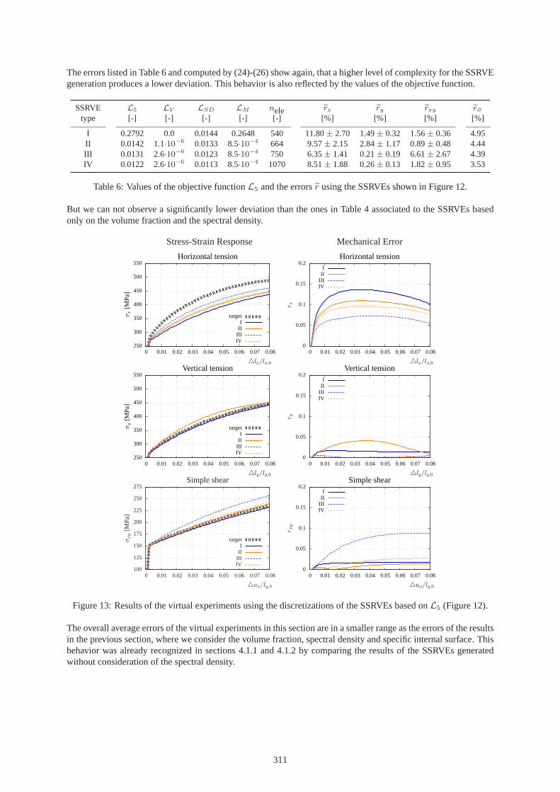
The errors listed in Table 6 and computed by (24)-(26) show again, that a higher level of complexity for the SSRVEgeneration produces a lower deviation. This behavior is also reflected by the values of the objective function.

SSRVE L5 LV LSD LM nele erx ery erxy er∅

type [-] [-] [-] [-] [-] [%] [%] [%] [%]

I 0.2792 0.0 0.0144 0.2648 540 11.80± 2.70 1.49± 0.32 1.56± 0.36 4.95II 0.0142 1.1·10−6 0.0133 8.5·10−4 664 9.57± 2.15 2.84± 1.17 0.89± 0.48 4.44III 0.0131 2.6·10−6 0.0123 8.5·10−4 750 6.35± 1.41 0.21± 0.19 6.61± 2.67 4.39IV 0.0122 2.6·10−6 0.0113 8.5·10−4 1070 8.51± 1.88 0.26± 0.13 1.82± 0.95 3.53


But we can not observe a significantly lower deviation than the ones in Table 4 associated to the SSRVEs basedonly on the volume fraction and the spectral density.


250

300

350

400

450

500

550

0 0.01 0.02 0.03 0.04 0.05 0.06 0.07 0.08

σx

[MP

a]

△lx/lx,0

Horizontal tension

targetI

IIIIIIV

0

0.05

0.1

0.15

0.2

0 0.01 0.02 0.03 0.04 0.05 0.06 0.07 0.08

r x

△lx/lx,0

Horizontal tensionI

IIIIIIV

250

300

350

400

450

500

550

0 0.01 0.02 0.03 0.04 0.05 0.06 0.07 0.08

σy

[MP

a]

△ly/ly,0

Vertical tension

targetI

IIIIIIV

0

0.05

0.1

0.15

0.2

0 0.01 0.02 0.03 0.04 0.05 0.06 0.07 0.08

r y

△ly/ly,0

Vertical tensionI

IIIIIIV

100

125

150

175

200

225

250

275

0 0.01 0.02 0.03 0.04 0.05 0.06 0.07 0.08

σxy

[MP

a]

△ux/ly,0

Simple shear

targetI

IIIIIIV

0

0.05

0.1

0.15

0.2

0 0.01 0.02 0.03 0.04 0.05 0.06 0.07 0.08

r xy

△ux/ly,0

Simple shearI

IIIIIIV


The overall average errors of the virtual experiments in this section are in a smaller range as the errors of the resultsin the previous section, where we consider the volume fraction, spectral density and specific internal surface. Thisbehavior was already recognized in sections 4.1.1 and 4.1.2by comparing the results of the SSRVEs generatedwithout consideration of the spectral density.

311

4.3 Combination of all four statistical measures

At least we consider all statistical measures which are discussed in this contribution. Using the objective func-tion (18), (22), (29) and (34) we formulate the minimizationproblem

L6(γ) = ωV LV (γ) + ωALA(γ) + ωMLM (γ) + ωSDLSD(γ) → min (38)

with ωV = ωA = ωM = ωSD = 1 ,

for the generation of the four different types of SSRVE. The results of the optimization process are depicted inFig. 14.


L6 = 0.2853 L6 = 0.0144 L6 = 0.0139 L6 = 0.0140


The stress-strain curves in Fig. 15 do not show better accuracies than the results from the previous section, wherewe do not consider the specific internal surface. On the contrary we can observe larger error values up to nearly17%in the horizontal tension test. Computing the average errors by (24)-(26) and listing them in Table 7 we see againthe worse results. Although the value of the objective function nearly decreases from one complexity level to thenext one, the overall average error does not show the same behavior.

SSRVE L6 LV LSD LS LM nele erx ery erxy er∅

type [-] [-] [-] [-] [-] [-] [%] [%] [%] [%]

I 0.2853 0.1653 0.0160 0.0301 0.0739 548 14.43± 3.30 2.97± 0.61 6.18± 2.23 7.86II 0.0144 2.9·10−7 0.0136 2.2·10−8 8.5·10−4 824 6.92± 1.55 0.40± 0.20 0.35± 0.29 2.56III 0.0139 1.1·10−6 0.0131 5.7·10−6 8.5·10−4 726 11.20± 2.55 1.62± 0.37 3.48± 1.52 5.43IV 0.0140 0.0 0.0132 2.2·10−8 8.5·10−4 1140 8.80± 1.94 1.69± 0.89 0.60± 0.35 3.70


4.4 Discussion

For a concluding discussion of the optimizations and the virtual experiments in the previous subsections we sum-marize the results in Table 8. The valuesLi of the corresponding objective function represent the optimizationlevel of accuracy of the generated SSRVE. Whereas, the overall average errorsr∅ describe the accuracy of thevirtual experiments of the SSRVEs compared with those of thetarget structure. At first we take a look at the over-all behavior of the least-square functionalsLi. In most of the cases we observe a decreasing value forLi alongwith an increasing number of sampling points and therewith increasing morphology complexity. This behaviorwas expected, as the number of sampling points represents the degree-of-freedoms for the minimization problemduring the SSRVE generation.The improvement of the mechanical error with a decreasing value of the minimal least-square functional is ob-served for the objective functions, where the spectral density is taken into account and where the specific internalsurface is not considered (L3 andL5). This indicates that the specific internal surface seems not to be a verysuitable statistical measure. Although the specific integral of mean curvature seems not to degrade the quality ofthe mechanical error when using the spectral density, it does also not improve the quality particularly. This can beseen for the examined microstructures by a more or less similar behavior with respect to the mechanical responseof the SSRVEs obtained from objective functionsL3 andL5. Comparing the overall average errors of the firstthree measure combinationsL1, L2 andL3 we notice that a suitable improvement of the mechanical error withincreasing complexity of the SSRVE is only obtained for the objective function where the spectral density is taken

312


250

300

350

400

450

500

550

0 0.01 0.02 0.03 0.04 0.05 0.06 0.07 0.08

σx

[MP

a]

△lx/lx,0

Horizontal tension

targetI

IIIIIIV

0

0.05

0.1

0.15

0.2

0 0.01 0.02 0.03 0.04 0.05 0.06 0.07 0.08

r x

△lx/lx,0

Horizontal tensionI

IIIIIIV

250

300

350

400

450

500

550

0 0.01 0.02 0.03 0.04 0.05 0.06 0.07 0.08

σy

[MP

a]

△ly/ly,0

Vertical tension

targetI

IIIIIIV

0

0.05

0.1

0.15

0.2

0 0.01 0.02 0.03 0.04 0.05 0.06 0.07 0.08r y

△ly/ly,0

Vertical tensionI

IIIIIIV

100

125

150

175

200

225

250

275

0 0.01 0.02 0.03 0.04 0.05 0.06 0.07 0.08

σxy

[MP

a]

△ux/ly,0

Simple shear

targetI

IIIIIIV

0

0.05

0.1

0.15

0.2

0 0.01 0.02 0.03 0.04 0.05 0.06 0.07 0.08

r xy

△ux/ly,0

Simple shearI

IIIIIIV


into account (L3). In addition, also the absolute values of the mechanical errors besides SSRVE type I, in particularfor the horizontal and vertical tension tests, are lower forL4. This is somehow obvious since a macroscopicallyanisotropic target structure is taken into account and the specific internal surface as well as the specific integral ofmean curvature are not able to cover directional information.

SSRVE L1 er∅ L2 er∅ L3 er∅ L4 er∅ L5 er∅ L6 er∅

type [-] [%] [-] [%] [-] [%] [-] [%] [-] [%] [-] [%]

I 0.0188 4.89 0.2647 4.77 0.0144 7.34 0.0343 7.32 0.2792 4.950.2853 7.86II 1.5·10−9 4.06 8.5·10−4 3.48 0.0133 3.78 0.0134 4.37 0.0142 4.44 0.0144 2.56III 1.5·10−9 5.32 8.5·10−4 4.43 0.0127 4.97 0.0131 5.42 0.0131 4.39 0.0139 5.43IV 2.4·10−10 3.40 8.5·10−4 4.47 0.0100 3.38 0.0132 5.94 0.0122 3.53 0.0140 3.70

Table 8: ValuesLi of the corresponding objective functions and the overall average errorsr∅ of the virtual exper-iments using the SSRVEs from all minimization problems 1-6.

5 Conclusion

In this contribution the applicability of different statistical measures describing the microstructural morphologytothe construction of statistically similar representativevolume elements (SSRVEs) were studied. The generation ofSSRVEs was based on the minimization of an ojective functionconsidering the difference of statistical measurescomputed from the “real” microstructure and the SSRVE. For an estimation of the possibility of the measures tocover mechanical information of the microstructure we compared the mechanical response of virtual experimentsperformed for the SSRVEs with those of the target structure.

313

As an important overall information of the morphology the volume fraction was firstly combined pairwise withthe specific internal surface, the specific integral of mean curvature and the spectral density. Then the spectraldensity turned out to be the most suitable parameter besidesthe volume fraction for the SSRVE generation andwas therefore combined with each of the both others for further studies. However, no improvement was observedwhen extending the objective function taking into account the spectral density and the volume fraction by one ofthe other basic parameters. In fact, even worse results wereobtained when using the specific internal surface.However, the spectral density turned out to be a suitable measure for the description of inclusion phase morphology,although further improvements are expectable by applying statistical measures of higher order as e.g. lineal-pathfunctions or three-point probability functions. In addition to that, the parameterization of the SSRVEs by splinesthat are generally permitted to transform arbitrarily in the search space needs to be investigated. Probably improvedresults can be expected when constraining the splines such that e.g. no intersections of individual splines areallowed.

Acknowledgement: The financial support of the “Deutsche Forschungsgemeinschaft” (DFG), research groupon “Analysis and Computation of Microstructure in Finite Plasticity”, project no. SCHR 570-8/1, is gratefullyacknowledged.

References

Balzani, D.; Schroder, J.: Some basic ideas for the reconstruction of statistically similar microstructures for multi-scale simulations.Proceedings in Applied Mathematics and Mechanics, 8, (2008), 10533–10534.

Balzani, D.; Schroder, J.; Brands, D.: FE2-simulation of microheterogeneous steels based on statistically similarRVE’s. In: Proceedings of the IUTAM Symposium on Variational Conceptswith applications to the mechanicsof materials, September 22-26, 2008, Bochum, Germany(2009a), in press.

Balzani, D.; Schroder, J.; Brands, D.; Carstensen, C.: Fe2-simulations in elasto-plasticity using statistically similarrepresentative volume elements.Proceedings in Applied Mathematics and Mechanics, in press.

Brekelmans, W.; Smit, R.; Meijer, H.: Prediction of the mechanical behaviour of nonlinear heterogeneous systemsby multi-level finite element modelling.Computer Methods in Applied Mechanics and Engineering, 155, (1998),181–192.

Conn, A. R.; Scheinberg, K.; Vicente, L. N.:Introduction to derivative-free optimization, vol. 8 of MPS/SIAMSeries on Optimization. Society for Industrial and Applied Mathematics (SIAM), Philadelphia, PA (2009).

Geers, M.; Kouznetsova, V.; Brekelmans, W.: Multi-scale first-order and second-order computational homoge-nization of microstructures towards continua.International Journal for Multiscale Computational Engineering,1, (2003), 371–386.

Hill, R.: Elastic properties of reinforced solids: some theoretical principles.Journal of the Mechanics and Physicsof Solids, 11, (1963), 357–372.

Klinkel, S.: Theorie und Numerik eines Volumen-Schalen-Elementes bei finiten elastischen und plastischen Verz-errungen. Ph.D. thesis, Universitat Fridericiana zu Karlsruhe (2000).

Kolda, T. G.; Lewis, R. M.; Torczon, V.: Optimization by direct search: new perspectives on some classical andmodern methods.SIAM Rev., 45, 3, (2003), 385–482 (electronic).

Kroner, E.: Allgemeine Kontinuumstheorie der Versetzung undEigenspannung.Archive of Rational Mechanicsand Analysis, 4, (1960), 273–334.

Lee, E.: Elasto-plastic deformation at finite strains.Journal of Applied Mechanics, 36, (1969), 1–6.

Makela, M. M.; Neittaanmaki, P.: Nonsmooth optimization. World Scientific Publishing Co. Inc., River Edge, NJ(1992).

Miehe, C.: Kanonische Modelle multiplikativer Elasto-Plastizitat. Thermodynamische Formulierung und Nu-merische Implementation.. Ph.D. thesis, Universitat Hannover, Institut fur Baumechanik und NumerischeMechanik, Bericht-Nr. F93/1 (1993), Habilitationsschrift.

Miehe, C.; Schroder, J.; Schotte, J.: Computational homogenization analysis in finite plasticity. simulation oftexture development in polycrystalline materials.Computer Methods in Applied Mechanics and Engineering,171, (1999), 387–418.

314

Miehe, C.; Stein, E.: A canonical model of multiplicative elasto-plasticity formulation and aspects of the numericalimplementation.European Journal of Mechanics, A/Solids, 11, (1992), 25–43.

Nelder, J. A.; Mead, R.: A simplex method for function minimization.The Computer Journal, 7, (1965), 308–313.

Ohser, J.; Mucklich, F.:Statistical analysis of microstructures in materials science. J Wiley & Sons (2000).

Parzen, E.:Stochastic processes. Holden-Day, San Francisco, Calif. (1992).

Peric, D.; Owen, D.; Honnor, M.: A model for finite strain elasto-plasticity based on logarithmic strains: Compu-tational issues.Computer Methods in Applied Mechanics and Engineering, 94, (1992), 35–61.

Povirk, G.: Incorporation of microstructural informationinto models of two-phase materials.Acta Metallurgica,43/8, (1995), 3199–3206.

Schramm, H.; Zowe, J.: A version of the bundle idea for minimizing a nonsmooth function: conceptual idea,convergence analysis, numerical results.SIAM J. Optim., 2, 1, (1992), 121–152.

Schroder, J.: Homogenisierungsmethoden der nichtlinearen Kontinuumsmechanik unter Beachtung von Sta-bilit atsproblemen. Ph.D. thesis, Bericht aus der Forschungsreihe des Institut fur Mechanik (Bauwesen),Lehrstuhl I (2000), Habilitationsschrift.

Schroder, J.; Balzani, D.; Richter, H.; Schmitz, H.; Kessler, L.: Simulation of microheterogeneous steels based ona discrete multiscale approach. In: P. Hora, ed.,Proceedings of the 7th International Conference and Workshopon Numerical Simulation of 3D Sheet Metal Forming Processes, pages 379–383 (2008).

Simo, J.: A framework for finite strain elastoplasticity based on maximum plastic dissipation and the multiplicativedecomposition: Part i. continuum formulation.Computer Methods in Applied Mechanics and Engineering, 66,(1988), 199–219.

Simo, J.: Algorithms for static and dynamic multiplicativeplasticity that preserve the classical return mappingschemes of the infinitesimal theory.Computer Methods in Applied Mechanics and Engineering, 99, (1992),61–112.

Simo, J.; Miehe, C.: Associative coupled thermoplasticityat finite strains: Formulation, numerical analysis andimplementation.Computer Methods in Applied Mechanics and Engineering, 96, (1992), 133–171.

Smit, R.; Brekelmans, W.; Meijer, H.: Prediction of the mechanical behavior of nonlinear heterogeneous systemsby multi-level finite element modeling.Computer Methods in Applied Mechanics and Engineering, 155, (1998),181–192.

Weber, G.; Anand, L.: Finite deformation constitutive equations and a time integration procedure for isotropic,hyperelastic-viscoelastic solids.Computer Methods in Applied Mechanics and Engineering, 79, (1990), 173–202.

Addresses:Dr.-Ing. Daniel Balzani, Institute of Mechanics and Computational Mechanics, Leibniz UniversityHannover, D-30167 Hannover.email:[email protected] Brands, Jorg Schroder, Institute of Mechanics, University of Duisburg-Essen, D-45117 Essen.email:[email protected], [email protected] Carstensen, Institute of Mathematics, Humboldt-University Berlin, D-10099 Berlin.email:[email protected]

315

sensitivity analysis of statistical measures for the ... · technische mechanik, 30, 4, (2010),...

Documents