Sensors and Microsystems

Piero Malcovati • Andrea Baschirotto

Editors

Sensors and Microsystems

AISEM 2009 Proceedings

Arnaldo D’Amico • Corrado di Natale

Editors Piero Malcovati Andrea Baschirotto

Università di Pavia Università Milano-Bicocca Via Ferrata, 1

piero.malcovati@unipv.it

ISBN 978-90-481-3605-6 e-ISBN 978-90-481-3606-3 DOI 10.1007/978-90-481-3606-3 Springer Dordrecht Heidelberg London New York

Library of Congress Control Number: 2009942133

© Springer Science + Business Media B.V. 2010 No part of this work may be reproduced, stored in a retrieval system, or transmitted in any form or by any means, electronic, mechanical, photocopying, microfilming, recording or otherwise, without written permission from the Publisher, with the exception of any material supplied specifically for the purpose ofbeing entered and executed on a computer system, for exclusive use by the purchaser of the work.

Printed on acid-free paper

Springer is part of Springer Science+Business Media (www.springer.com)

Dipartimento di Ingegneria Ele ttrica

Piazza della Scienza, 3 27100 Pavia 20126 Milano

andrea.baschirotto@unimib.it Italy Italy

Dipartimento di Fisica

dinatale@eln.uniroma2.it

Arnaldo D’Amico Corrado di Natale

Via del Politecnico, 1 00133 Roma Italy damico@eln.uniroma2.it

Dipartimento di Elettronica Università di Roma, Tor Vergata

Via del Politecnico, 1 00133 Roma Italy

Dipartimento di Elettronica Università di Roma, Tor Vergata

v

FOREWORD

This book is the collection of most of the papers presented at the 14th Italian

Conference on Sensors and Microsystems, promoted by the Italian Association on Sensors and Microsystems (AISEM). This Conference edition, organized by the University of Pavia, was held from 24th to 26th

February 2009 in the

historical Aula Foscolo of the University of Pavia. The book includes also three tutorial papers, which address basic concepts in the area of sensors and microsystems.

The 2009 AISEM Conference edition was opened by the Rector of the University of Pavia, Prof. Angiolino Stella, who is well known for his research activity in the sensor and microsystems community. Moreover, this edition was characterized by four important invited talks from the industrial world, which demonstrated the successful exploitation of the research in the field of sensors and microsystems.

Benedetto Vigna (STMicroelectronics) illustrated the strategy, both at technical and management level, that allowed STMicroelectronics to become in 2009 the world leader in the MEMS market. Christoph Hagleitner (IBM Research Zurich) described the recent development of the “Millipede Project”, that uses a nanotechnology approach to increase the performance of data storage systems. Marco Sabatini (Pirelli) explained the application of several microsensor techniques in the realization of a Cyber-Tyre under development at Pirelli. Finally, Giorgio Fagnani (Gefran Sensori) spoke about the recent developments on sensors for pressure measurements at high temperature.

More than 100 researchers participated to the event ,organized with both oral and poster sessions. At the end of the Conference, two awards were delivered for the best paper and the best posters.

The Best Paper Award entitled to Angelo Rizzo, aimed to support young researchers, sponsored by CNR-IMM and delivered by Dr. Pietro Siciliano, was assigned to Marco Grassi for the paper “A Multisensor System for High Reliability People Fall Detection in Home Environment”.

The Best Poster Award, sponsored by the Conference Organization, was assigned ex-aequo to the papers “Actively Controlled Power Conversion Techniques for Piezoelectric Energy Harvesting Applications” by A. Romani, C.

Foreword vi

Tamburini, R. P. Paganelli, A. Golfarelli, R. Codeluppi, M. Dini, E. Sangiorgi, M. Tartagni and “A Novel Based Protein Microarray for the Simultaneous Analysis of Activated Caspases” by I. Lamberti, L. Mosiello, C. Cenciarelli, A. Antoccia, C. Tanzarella.

Special thanks are given to Dr. Alessandro Cabrini of the University of Pavia for his effort and dedication in the organization of the Conference.

Andrea Baschirotto Università di Milano-Bicocca

Piero Malcovati Università di Pavia

Arnaldo D’Amico, Corrado Di Natale Università di Roma “Tor Vergata”

Conference Chairman

Prof. Andrea Baschirotto Università di Milano-Bicocca

Prof. Piero Malcovati Università di Pavia

Local Organization Chairman

Dr. Alessandro Cabrini Università di Pavia

AISEM Directive Committee

A. D’Amico Università di Roma

“Tor Vergata” Presidente AISEM

L. Campanella Università di Roma

“La Sapienza”

P. Siciliano CNR-IMM Lecce

C. Mari Università di Milano

G. Martinelli Università di Ferrara

U. Mastromatteo STMicroelectronics

A. G. Mignani CNR-IFAC Firenze

M. Prudenziati Università di Modena

G. Sberveglieri Università di Brescia

G. Soncini Università di Trento

AISEM COMMITTEES

Technical Program Chairman

AISEM Scientific Committee

M. C. Carotta

Università di Ferrara

P. Dario Scuola Superiore S. Anna

Pisa

F. Davide Telecom Italia Roma

A. Diligenti Università di Pisa

C. Di Natale Università di Roma

“Tor Vergata”

L. Dori CNR-IMM-LAMEL

Bologna G. Faglia

Università di Brescia C. Malvicino

CR Fiat Orbassano (To) G. Martinelli

Università di Ferrara

M. Mascini Università di Firenze

N. Minnaja Polo Navacchio Cascina

(PI)

B. Morten Università di Modena

G. Palleschi Università di Roma

“Tor Vergata”

F. Villa STMicroelectronics

M. Zen FBK Trento

ix

TABLE OF CONTENTS

Tutorials

With the Eye of the Beholder: An Introduction to the Observation of Multidimensional Data with the Principal Component Analysis .....................3 C. Di Natale Biosensor Technology: A Brief History .............................................................15 I. Palchetti and M. Mascini Fundamental Limitations in Resistive Wide-Range Gas-Sensor Interface Circuits Design....................................................................................................25 M. Grassi, P. Malcovati and A. Baschirotto

Materials and Processes

Advances in Silicon Periodic Microstructures with Photonic Band Gaps in the Near Infrared Region ................................................................................43 G. Barillaro, A. Diligenti, L. M. Strambini, V. Annovazzi-Lodi, M. Benedetti, S. Merlo and S. Riccardi Investigation of the Swelling Properties of PHEMA and PHEMA/CB for Sensing Application ......................................................................................47 V. La Ferrara, E. Massera, M. L. Miglietta, T. Polichetti, G.Rametta and G. Di Francia Optical Sensing Properties Towards Ethanol Vapors of Au-Polyimide Nanocomposite Films Synthesized by Different Chemical Routes....................51 S. Carturan, A. Antonaci, G. Maggioni, A. Quaranta, M. Tonezzer, R. Milan, G. Mattei and P. Mazzoldi Optical Vapors Sensing Capabilities of Polymers of Intrinsic Microporosity ..55 S. Carturan, A. Antonaci, G. Maggioni, A. Quaranta, M. Tonezzer, R. Milan and G. Della Mea Focused Ion Beam and Dielectrophoresis as Grow-in-Place Architecture for Chemical Sensor............................................................................................59 V. La Ferrara, B. Alfano, E. Massera and G. Di Francia,

Table of Contents x

A Novel Approach for the Preparation of Metal Oxide/CNTs Composites for Sensing Applications.....................................................................................63 G. Neri, A. Bonavita, G. Micali, G. Rizzo, M.- G. Willinger, E. Rauwel and N. Pinna The impact of Nanoparticle Aggregation in Liquid Solution for Toxicological and Ecotoxicological Studies ..............................................................................67 M. L. Miglietta, G. Rametta, G. Di Francia, A. Bruno, C. De Lisio, G. Leter, M. Mancuso, F. Pacchierotti, S. Buono and S.Manzo Preparation and Electrical-Functional Characterization of Gas Sensors Based on TIO2 Nanometric Strips Using Impedance Spectroscopy..............................71 C. De Pascali, L. Francioso, S. Capone and P. Siciliano Piezoelectric Low-Curing-Temperature Ink for Sensors and Power Harvesting ...........................................................................................................77 M. Ferrari, V. Ferrari, M. Guizzetti and D. Marioli Comparative Bioaffinity Studies for In-Vitro Cell Assays on MEMS-Based Devices ................................................................................................................83 C. Ress, L. Odorizzi, C. Collini, L. Lorenzelli, S. Forti, C. Pederzolli, L. Lunelli, L. Vanzetti, N. Coppedè, T. Toccoli, G.Tarabella and S. Iannotta Effect of the Layer Geometry on Ink-Jet Sensor Device Perfomances ..............89 A. De Girolamo Del Mauro, F. Loffredo, G. Burrasca, E.Massera, G. Di Francia and D. Della Sala

Devices

Optical Flowmeter Sensor for Blood Circulators ...............................................97 M. Norgia, A. Pesatori and L. Rovati UV Laser Beam Profilers Based on CVD Diamond.........................................101 M. Girolami, P. Allegrini, G. Conte and S. Salvatori Photoconductive Position Sensitive CVD Diamond Detectors ........................105 M. Girolami, P. Allegrini, G. Conte and S. Salvatori Opaque-Gate Phototransistors on H-Terminated Diamond..............................109 P. Calvani, M. C. Rossi and G. Conte Fabrication and Characterization of a Silicon Photodetector at 1.55 Micron ...................................................................................................113 M. Casalino, L. Sirleto, M. Gioffre, G. Coppola, M. Iodice, I.Rendina and L. Moretti

Table of Contents xi

Active Area Density Optimization Technique for Harvester Photodiodes Efficiency Maximization...................................................................................117 E. Dallago, M. Ferri, P. Malcovati and D. Pinna All-Fiber Hybrid Fiber Bragg Gratings Cavity for Sensing Applications........121 D. Paladino, G. Quero, A. Cutolo, A. Cusano, C. Caucheteur and P. Megret An Optical Platform Based on Fluorescence Anisotropy for C Reactive Protein and Procalcitonine Assay .....................................................................127 F. Baldini, A. Giannetti, F. Senesi, C. Trono, L. Bolzoni and G.Porro Gold Coated Long Period Gratings in Single and Multi Layer Configuration for Sensing Applications ...........................................................133 A. Iadicicco, S. Campopiano, D. Paladino, A. Cutolo, A.Cusano and W. Bock UV Schottky Sensors Based on Wide Bandgap Semiconductors.....................137 P. Allegrini, P. Calvani, M. Girolami, G. Conte and M. C. Rossi Design and Realization of a Novel Pixel Sensor for Color Imaging Applications in CMOS 90 nm Technology ......................................................143 G. Langfelder, A. Longoni and F. Zaraga Technology and I-V Characteristics of Fully Porous PN Junctions..................147 N. Bacci, G. Barillaro and A. Diligenti Fast Gating of Single-Photon Avalanche Diodes for Photon Migration Measurements ...................................................................................................151 A. Dallamora, A. Tosi, F. Zappa, S. Cova, A. Pifferi, A.Torricelli, L. Spinelli, D. Contini and R. Cubeddu Performance of Commercially Available InGaAs/InP Spad with Custom Electronics.........................................................................................................155 A. Tosi, A. Dalla Mora, F. Zappa and S. Cova Novel Vacuum Evaporated Cavitand Sensors for Detecting Very Low Alcohol Concentrations.....................................................................................161 M. Tonezzer, G. Maggioni M. Melegari and E. Dalcanale Hydrogen Sensing Capability of Nanostructured Titania Films.......................165 G. Micali, A. Bonavita, G. Neri, G. Centi, S. Perathoner, R.Passalacqua and N. Donato Synthesis and Gas Sensing Properties of ZnO Quantum Dots .........................169 A. Forleo, L. Francioso, S. Capone, P. Siciliano and P. Lommens

Table of Contents xii

Optical Gas Sensing Properties of ZnO Nanowires..........................................173 S. Todros, C. Baratto, E. Comini, G. Faglia, M. Ferroni, G.Sberveglieri S.Lettieri, A. Setaro, L. Santamaria and P. Maddalena Porphyrin-Porphyrin Diads as Potential Transducers for the Determination of Cadaverine in Aqueous Solution ..................................................................177 F. Baldini, A. Giannetti, C. Trono, T. Carofiglio and E. Lubian Electrochemical Characterization of PNA/DNA Hybridized Layer Using SECM and EIS Techniques...............................................................................181 I. Palchetti, F. Berti, S. Laschi, G. Marrazza and M. Mascini Metal-Functionalized and Vertically-Aligned Multi walled Carbon Nanotube Layers for Low Temperature Gas Sensing Applications .................185 M. Penza, R. Rossi, M. Alvisi, M. A. Signore, G. Cassano, R. Pentassuglia, D. Suriano, V. Pfister and E. Serra Ammonia Sensing Properties of Organic Inks Deposited on Flexible Subtrates ............................................................................................................193 A. Arena, N. Donato, G. Saitta, G. Rizzo and G. Neri Prospective of Using Nano-Structured High Performances Sensors Based on Polymer Nano-Imprinting Technology for Chemical and Biomedical Applications ......................................................................................................197 A. Ferrario, A. De Toni, L. Bandiera and M. Quarta Surface Acoustic Wave Biosensor Based on a Recombinant Bovine Odorant-Binding Protein...................................................................................201 F. Di Pietrantonio, I. Zaccari, M. Benetti, D. Cannatà, E. Verona, R. Crescenzo, V. Scognamiglio and S. D’Auria Development of an Aptamer-Based Electrochemical Sandwich Assay for the Detection of a Clinical Biomarker.........................................................207 S. Centi, S. Tombelli, I. Palchetti and M. Mascini Determination of Ethanol in Leadless Petrols and Biofuels Using an Innovative Organic Phase Enzyme Electrode (OPEE) ...............................211 L. Campanella, G. S. Capesciotti, T. Gatta and M. Tomassetti Immunosensors for the Direct Determination of Proteins: Lactoferrin and HIgG...........................................................................................................215 L. Campanella, E. Martini and M. Tomassetti

Table of Contents xiii

A Method Based on Scattering Parameters for Model Identification of Piezoactuators with Applications in Colloidal Suspension Monitoring.........................................................................................................219 R. P. Paganelli, A. Golfarelli, A. Romani, M. Magi and M. Tartagni MEMS Tilt Sensor with Improved Resolution and Low Thermal Drift...........225 D. Crescini, M. Baù and V. Ferrari An Offset Compensation Method for Integrated Thermal Flow Sensors.........229 P. Bruschi, M. Dei and M. Piotto A New Principle for Environment Resistant Integrated Anemometers............233 P. Bruschi, M. Dei and M. Piotto Distributed Dynamic Strain Measurement Using a Time-Domain Brillouin Sensing System..................................................................................237 R. Bernini, A. Minardo and L. Zeni Epoxy/MWCNT Composite Based Temperature Sensor with Linear Characteristics ...................................................................................................241 H. C. Neitzert, A. Sorrentino and L. Vertuccio Thermoelectric Sensor for Detection of Chemical Radiation Heat ..................247 A. Catini, E. Gioia, E. Girolami, L. Spagnolo, C. Di Natale, A. D’Amico, M. Bari and L. Ahmad Squid Sensors for High Spatial Resolution Magnetic Imaging and for Nanoscale Applications ........................................................................251 A. Vettoliere, C. Granata, P. Walke, E. Esposito, B. Ruggiero and M. Russo Perming Effect in Residence Times Difference Fluxgate Magnetometers.......257 B. Ando, S. Baglio, S. La Malfa, C. Trigona and A. R. Bulsara Diffuse-Light Absorption Spectroscopy by Means of a Fiber Optic Supercontinuum Source – An Innovative Technique .......................................261 A. G. Mignani, L. Ciaccheri, I. Cacciari, H. Ottevaere, H. Thienpont, O. Parriaux and M. Johnson

Systems

A Differential Difference Current-Conveyor (DDCCII) Based Front-End for Integrable and Portable Sensor Applications.............................267 A. De Marcellis, C. Di Carlo, G. Ferri, V. Stornelli, A. D’Amico, C. Di Natale and E. Martinelli

Table of Contents xiv

A New Fast-Readout Front-End for High Resistive Chemical Sensor Applications ......................................................................................................273 A. Depari, A. Flammini, D. Marioli, E. Sisinni, A. De Marcellis, G. Ferri and V. Stornelli A Novel Calibration-Less CCII-Based Resistance-to-Time Front-End for Gas Sensor Interfacing ................................................................................279 A. De Marcellis, C. Di Carlo, G. Ferri, V. Stornelli, A. Depari, A. Flammini and D. Marioli High-Efficiency Front-End Interface for the Vibrating-String Strain Gauge Sensors...................................................................................................285 A. Simonetti and A. Trifiletti Signal Conditioning System Analysis for Adaptive Signal Processing in Wireless Sensors ...........................................................................................291 L. Barboni and M. Valle A 0.13μm CMOS Front-End for Drift Chambers .............................................295 S. D’Amico, A. Baschirotto M. De Matteis, F. Grancagnolo, M. Panareo, R. Perrino, G. Chiodini and A. Corvaglia A New Laser Technology for Air Traffic Management ...................................299 M. Salerno, G. Costantini, M. Carota, D. Casali, D. Rondinella and M. V. Crispino A 100Microwatt Ultra Low-Power Contrast-Based Asynchronous Vision Sensor ................................................................................................................303 N. Massari, M. Gottardi, S. A. Jawed and G. Soncini A 32 x 32-Channels Chip for X-Ray Pixel Detector Read-Out........................307 M. Grassi, V. Ferragina, P. Malcovati, S. Caccia, G.Bertuccio, D. Martin, P. Bastia, I. Cappelluti and N. Ratti Mental Tasks Recognition for a Brain/Computer Interface..............................311 G. Costantini, D. Casali, M. Carota, G. Saggio, L. Bianchi, M. Abbafati and L. Quitadamo Silicon Integrated Micro-Balances Array for DNA Hybridization Electronic Detection ...........................................................................................................315 G. Barlocchi, U. Mastromatteo and F. Villa A Fully Integrated System for Single-Site Electroporation and Addressed Cell Drug Delivery............................................................................................319 L. Odorizzi, C. Collini, E. Morganti, R. Cunaccia, C. Ress, L. Lorenzelli, A. Gianfelice, E. Jacchetti, C. Lenardi and P. Milani

Table of Contents xv

A Novel Based Protein Microarray for the Simultaneous Analysis of Activated Caspases .......................................................................................323 I. Lamberti, L. Mosiello, C. Cenciarelli, A. Antoccia and C.Tanzarella Electrorheological Fluids Based on Inorganic Nanoparticles for Robotic Applications ......................................................................................................327 L. Scibilia, G. Rizzo, M. Sorrenti, G. Neri, P. Giorgianni, M. Levanti and S.S. Marchese Wireless Nanotransducers for In-Vivo Medical Applications..........................331 G. Mantini, A. D’Amico, C. Falconi and Z. Lin Wang Development of MEMS Microcantilever Detectors for DNA Single Nucleotide Polymorphism Detection in Autoimmune Diseases Diagnostic .........................................................................................................335 A. Adami, M. Decarli, L. Odorizzi, L. Lorenzelli, K. Fincati, K. Schicho and H. Gruessinger A New Approach for CMOS Fabrication of Microcantilever/Nanotip Systems for Probe-Storage Applications ..........................................................339 G. Barillaro, S. Surdo and G. M. Lazzerini Characterization and Testing of a Double Axis Scanning Micromirror...........343 F. Battini, E. Volpi, E. Marchetti, T. Cecchini, F. Sechi, L. Fanucci, M. De Marinis and U. Hofmann A High-Voltage PWM Current Driver for Hot-Wire Anemometers................347 E. Volpi, L. Fanucci, F. D’Ascoli and E. Pardi A MEMS Piezoresistive Inclination Sensor with CMOS ASIC Front-End Interface.............................................................................................................353 S. Dalola, V. Ferrari and D. Marioli Actively Controlled Power Conversion Techniques for Piezoelectric Energy Harvesting Applications....................................................................................359 A. Romani, C. Tamburini, A. Golfarelli, R.Codeluppi, M. Dini, E. Sangiorgi, M. Tartagni and R. P. Paganelli FEM Analysis of Piezoelectric Nanostructures for Energy Harvesting ...........365 G. Mantini, A. D’Amico, C. Falconi, Z. Lin Wang Piezo-polymer-Fet Devices Based Tactile Sensors for Humanoid Robots ......369 R. S. Dahiya, G. Metta, M. Valle, L. Lorenzelli and A. Adami Integrated Optofluidic Mach-Zehnder Interferometer ......................................373 R. Bernini, G. Testa, L. Zeni and P. M. Sarro

Table of Contents xvi

Intelligent Wireless E-Nose for Power Savvy Distributed Chemical Sensing ..............................................................................................................377 S. De Vito, E. Massera, G. Burrasca, A. De Girolamo and G. Di Francia SmartRFID-Label for Monitoring the Preservation Conditions of Food .........381 D. Cartasegna, A. Cito, F. Conso, A. Donida, M. Grassi, L. Malvasi, G. Rescio and P. Malcovati Improving Piano Music Transcription by Elman Dynamic Neural Networks ...........................................................................................................387 G. Costantini, M. Todisco and M. Carota A Multisensor System for High Reliability People Fall Detection in Home Environment......................................................................................................391 M. Grassi, A. Lombardi, G. Rescio, P. Malcovati, A. Leone, G. Diraco, C. Distante, P. Siciliano, M. Malfatti, L. Gonzo, V. Libal, J. Huang and G. Potamianos

Applications

WESNEP: A Wireless Environmental Sensor Network for Permafrost Studies ...............................................................................................................397 A. Cristiani, G. M. Bertolotti, G. Beltrami, R. Gandolfi, R.Lombardi, R. Seppi and F. Zucca A Multi-Purpose Wireless Sensor Network Based on Zigbee Technology........................................................................................................401 G. M. Bertolotti, G. Beltrami, A. Cristiani, G. Gandolfi and R.Lombardi A Wireless Sensors System for Sport Studies ..................................................405 G. M. Bertolotti, G. Beltrami, A. Cristiani, G. Gandolfi and R. Lombardi A High-Voltage Driver for a Scanning Micromirror........................................409 E. Volpi, L. Fanucci and F. D’Ascoli System Study for a Head-Up Display Based on a Flexible Sensor Interface.............................................................................................................413 E. Volpi, F. Sechi, T. Cecchini, F. Battini, L. Bacciarelli, L. Fanucci and M. De Marinis Capacitive Sensor System for Investigation of Two-Phase Flow in Pipes.....................................................................................................419 M. Demori, V. Ferrari and D. Strazza

Table of Contents xvii

Surface Plasmon Resonance Imaging for Affinity-Based Biosensors..............425 S. Scarano C. Suffi, M. Mascini and M. Minunni, Laser Based Scanning System for Monitoring Ice Accretion Phenomena on High Voltage Conductors.............................................................................429 E. Golinelli, U. Perini, S. Musazzi and G. Pirovano Capacitive Proximity Sensor for Chainsaw Safety...........................................433 M. Norgia and C. Svelto Author Index....................................................................................................437

TUTORIALS

P. Malcovati et al. (eds.), Sensors and Microsystems: AISEM 2009 Proceedings, 3 Lecture Notes in Electrical Engineering 54, DOI 10.1007/978-90-481-3606-3_1, © Springer Science+Business Media B.V. 2010

WITH THE EYE OF THE BEHOLDER: AN INTRODUCTION TO THE OBSERVATION OF MULTIDIMENSIONAL DATA

WITH THE PRINCIPAL COMPONENT ANALYSIS

C. DI NATALE Deparment of Electronic Engineering, University of Rome “Tor Vergata”. Via del

Politecnico 1,00133 Roma, Italy, e-mail: dinatale@uniroma2.it

1. Data, patterns, matrices, and vector spaces

The graphical representation of experimental data is one of the most important and immediate approaches for the interpretation of scientific experiments. The process of description of data in a geometrical space is guided by some fundamental assumptions. For instance the connection of experimental data with points in a Euclidean space is the basic operation for any data representation. It is out of the scope of this paper to discuss the consequences of the introduction of non-Euclidean spaces, but it would be interesting to reflect that in the last century several demonstrations about the physical meaning of non-Euclidean spaces were provided.

Data are elementary entities that describe partial aspects of a phenomenon. When physical quantities are involved, data are the results of the application of pre-determined measurement instruments to the phenomenon under study. Measure-ment instruments and their measured quantities are predefined entities that are used, with the same meaning, in very different context. Let us consider, for instance, the measure of length; this can be applied to measure the height of an individual or the distance traveled by a vehicle. The resulting data will be formally the same but their meaning is, of course, extremely different. In some case such a data will not be adequate to describe a phenomena, as it will be discussed later.

Abstract. Multivariate data analysis is the necessary tool to study complex phenomena and to analyze data of complex analytical techniques such as chromatography and spectro-photometer. One of the most useful approaches in science to experimental data interpret-ation is the visualization of data. This fundamental operation cannot be simply performed with multivariate data. In this paper, an introduction to principal component analysis is offered as one of the method that can provide a meaningful representation of data in a projection plane. The choice of the projection plane corresponds to the determination of an optimal point of observation where multidimensional data can display most of their meaning.

C. Di Natale

4

by a ruler. The treatment of scalar (or univariate) data is well known and it is a background provided by any scientific or technical training.

In this paper the description of multivariate data will be considered. Multivariate data are provided either by multidimensional instruments or collecting together a number of univariate data in order to describe complex phenomena.

Multidimensional instruments are those measurement systems that, as a result of a measure, provide a sequence of ordered numerical quantities. Examples of this are gas-chromatographers, spectrophotometers, or sensor arrays and in particular those particular classes of arrays of partially selective sensors known as electronic noses. On the other hand, the description of complex phenomena req-uires the use of many individual data. As an example, to define the meteorological conditions is necessary to get at the same time data about the atmospheric pressure, the magnitude and direction of wind, the temperature, the relative humidity and so on.

Multivariate data are naturally composed in ordered sequences that are called patterns. The mathematical entity suitable to represent collections of patterns is the matrix. Linear algebra is then utilized to manipulate the patterns [1]. In this context the known relationship between matrices and vector spaces is also utilized to describe pattern. In practice, each pattern is associated to a vector in a suitable Euclidean vector where each basis vector is one of the dimensions of the multivariate data.

It is important to consider that observations take place at dimension 2, and then when the dimension is larger than 2, in order to observe the data is necessary to consider the point of view of the observation. This is a common knowledge that the perception of a three-dimensional object may change according to the point of view. As well known to any person taking a photograph there is a set of optimal point of views where the interesting aspects of an object can be projected onto the camera focal plane.

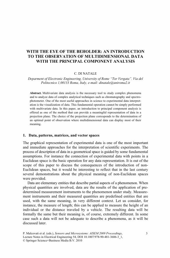
As an example, let us consider for instance a set of peaches of different cultivars for which the following parameters have been measured: total antocyanins content, brix degree, chlorophyll content, details about this experiment are found in [2]. In Fig. 1 the data, plotted in a three dimensional Euclidean space, are observed from two different points of view. It is straightforward that different points of view allows for different appreciation of the characteristics of the studied samples. For instance data points cluster in three groups in one case and in two groups in the other.

In the following of this paper the observation of patterns of dimensions larger than 3 will be discussed. Even if the original space goes beyond a sensible appraisal, the method is the same described for the display of data of dimension 3 and namely the projection from a point of observation onto a plane.

A great difference about data is related to their dimension. Simple data are scalar quantities complemented by a unit of measure, such as the data provided

With the Eye of the Beholder

5

Figure 1. Observation of the same data set from different points of view reveals or conceal the relationship between the data.

2. Data correlation

In the previous section it has been mentioned that the kind of data that can be acquired from a given phenomenon is predefined and it is limited to the set of quantities that are measurable. This means that for a specific phenomenon a sort of inadequacy of the measurable data can emerge. The inadequacy of data is manifested by the fact that different quantities tend to describe the same aspect of a phenomenon. In practice, it appears that a phenomenon is described by a set of internal processes that affects, at the same time, quantities that are physically different among them. To elucidate this point let us consider the following example. Let us suppose to consider a population of individuals and to measure for each of them the height and the weight. From a physical point of view length and mass are distinct quantities, and actually they are part of the three basic quantities from which all the other mechanical units of measure are formed. If the collected data are considered to form patterns and if these patterns are plotted in a bidimensional plane it is likely to observe that the points are almost aligned along a line. This means that the two data are in some way related one each other, in particular if an individual has a large weight it probably has a large height too. The connection between height and weight is absolutely not due to the nature of the measured quantity but rather to the fact that humans are characterized by law according to which the body mass tend to be vertically distributed. Deviations from this general trend indicate the peculiar properties of each individual that tend to derogate from the common law.

Data connected each other by an internal mutual dependence are said correlated. The degree of correlation is measured, for instance, by the linear correlation coefficient. Correlation can be either positive or negative describing if at a positive growth of one variable corresponds an increment or a decrement of the other. The correlation coefficient takes value from −1 to +1 indicating with ±1 positive and negative correlation and with 0 the absence of correlation.

Given a matrix of patterns, the calculus of the mutual correlation coefficients Provides evidences about the existence of internal relationships connecting variables among them. It is worth to mention that these kinds of conclusions

C. Di Natale

6

derive exclusively from an observation of data and they have to be corroborated and explained by the science pertaining to the kind of considered phenomenon. The mutual correlation coefficients can be arranged in a matrix called correlation matrix. Of course the matrix is symmetric (the correlations between variables 1 and 2, and variables 2 and 1, are obviously the same) with 1 along the main diagonal (each variable is correlated to itself).

Let us consider as an example an extension of the pattern matrix previously introduced about a population of peaches. For each peach the following quantities have been measured: acidity, antocyanins, brix, carotene, and chlorophyll. The correlation matrix of these data is shown in Table 1.

Table 1. Correlation matrix of a number of variables measured in a population of peaches.

Acid Antoc. Brix Carot. Chloroph. Acid 1.00 −0.48 0.34 0.15 −0.32 Antoc. −0.48 1.00 −0.70 −0.56 0.88 Brix 0.34 −0.70 1.00 0.30 −0.76 Carot. 0.15 −0.56 0.30 1.00 −0.25 Chloroph. −0.32 0.88 −0.76 −0.25 1.00

The correlation coefficients suggest for instance that since the couple anto-

cyanins and chlorophyll are largely correlated, the color of peaches is a blend of red and green. Another suggestion comes from the negative correlation of the couple chlorophyll and brix degree indicating that green peaches are not sweet.

In terms of data appearance in the Euclidean space, the existence of correlation indicates that the data point tend to be aligned along a line. Then two correlated quantities instead of uniformly filling the space tend to occupy a space volume that is more than unidimensional but not completely bidimensional. This characteristic influences greatly the determination of an optimal point of view where multidimensional data can be observed preserving the relationship between the data.

3. Principal component analysis

Principal Component Analysis (PCA) is a method to decompose a set of multivariate patterns into non-correlated variables [3]. In practice, PCA defines for a given set of multivariate data a number of novel variables that are not directly measurable but are defined as a linear combination of measurable variables. The main property of these novel variables (called principal components) is their non-correlation. They can be interpreted as a sort of virtual data each describing non-correlated properties of the phenomenon under study. The contribution to each principal component of the original measured quantities helps in under-standing the processes occurring in the phenomenon as it will be clear in the example that will be discussed later.

The calculus of PCA is based on the statistical properties of the whole set of patterns. For this reason it is necessary, before to discuss PCA, to introduce the

With the Eye of the Beholder

7

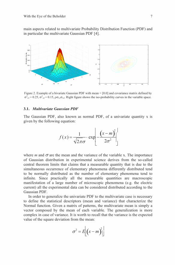
main aspects related to multivariate Probability Distribution Function (PDF) and in particular the multivariate Gaussian PDF [4].

Figure 2. Example of a bivariate Gaussian PDF with mean = [0.0] and covariance matrix defined by σ2

x1 = 0.25, σ2

x2 = 0.15, ρσx1σx2. Right figure shows the iso-probability curves in the variable space.

3.1. Multivariate Gaussian PDF

The Gaussian PDF, also known as normal PDF, of a univariate quantity x is given by the following equation:

f ( x) =1

2πσ⋅ exp −

x − m( )2

2σ 2

⎡

⎣

⎢ ⎢

⎤

⎦

⎥ ⎥

where m and σ are the mean and the variance of the variable x. The importance of Gaussian distribution in experimental science derives from the so-called central theorem limits that claims that a measurable quantity that is due to the simultaneous occurrence of elementary phenomena differently distributed tend to be normally distributed as the number of elementary phenomena tend to infinite. Since practically all the measurable quantities are macroscopic manifestation of a large number of microscopic phenomena (e.g. the electric current) all the experimental data can be considered distributed according to the Gaussian PDF.

In order to generalize the univariate PDF to the multivariate case is necessary to define the statistical descriptors (mean and variance) that characterize the Normal function. Given a matrix of patterns, the multivariate mean is simply a vector composed by the mean of each variable. The generalization is more complex in case of variance. It is worth to recall that the variance is the expected value of the square deviation from the mean:

σ 2 = E x − m( )2⎡

⎣ ⎢ ⎤ ⎦ ⎥

C. Di Natale

8

When x is a vector the previous definition becomes:

Σ = σ ij

2 = E xi − m( )T⋅ x j − m( )⎡

⎣ ⎢ ⎤ ⎦ ⎥

Where the indexes i and j go from 1 to the number of variables. The previous definition gives rise to a symmetric square matrix where the diagonal contains the variances of single variables and the other positions are proportional to the correlation coefficient according to the following equation:

Σij = ρij ⋅σ i ⋅σ j Figure 2 shows a bivariate Gaussian PDF with evidenced the iso-probability surfaces (in this case curves). These curves are defined by the quadratic form built with the covariance matrix.

x − x y − y [ ]⋅

σ x2 ρxyσ xσ y

−ρxyσ xσ y σ y2

⎡

⎣ ⎢ ⎢

⎤

⎦ ⎥ ⎥ ⋅

x − x y − y

⎡

⎣ ⎢

⎤

⎦ ⎥ = k

Since the covariance matrix is symmetric, according to the properties of quadratic forms, the iso-probability curves of bivariate Gaussian PDF are ellipse, in case of multivariate Gaussian PDF the iso-probability curves are ellipsoids.

3.2. Covariance matrix and principal components

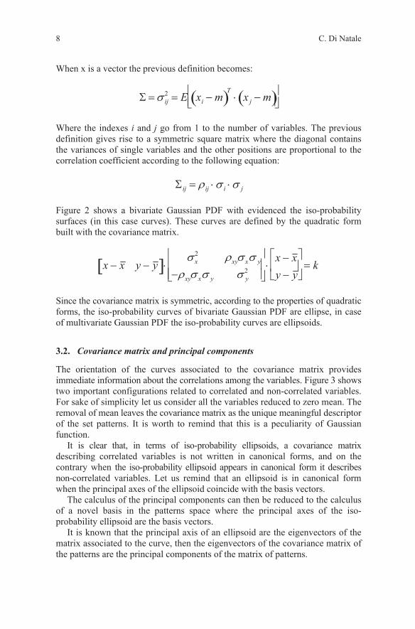
The orientation of the curves associated to the covariance matrix provides immediate information about the correlations among the variables. Figure 3 shows two important configurations related to correlated and non-correlated variables. For sake of simplicity let us consider all the variables reduced to zero mean. The removal of mean leaves the covariance matrix as the unique meaningful descriptor of the set patterns. It is worth to remind that this is a peculiarity of Gaussian function.

It is clear that, in terms of iso-probability ellipsoids, a covariance matrix describing correlated variables is not written in canonical forms, and on the contrary when the iso-probability ellipsoid appears in canonical form it describes non-correlated variables. Let us remind that an ellipsoid is in canonical form when the principal axes of the ellipsoid coincide with the basis vectors.

The calculus of the principal components can then be reduced to the calculus of a novel basis in the patterns space where the principal axes of the iso-probability ellipsoid are the basis vectors.

It is known that the principal axis of an ellipsoid are the eigenvectors of the matrix associated to the curve, then the eigenvectors of the covariance matrix of the patterns are the principal components of the matrix of patterns.

With the Eye of the Beholder

9

Figure 3. Examples of iso-probability ellipses occurring in case of correlated (left) and non-correlated (right) variables.

Besides the eigenvectors, the associated eigenvalues defines the importance of each principal component. Eigenvalues provide a measure of the elongation of the ellipse along the associated eigenvectors and it is a measure of the variance explained by each principal component. Indeed, since the principal components are non-correlated the total variance of the data set is given by the sum of the variances along each principal component. Therefore, the eigenvalues measure the “importance” of each associated principal components.

In practice the calculus of PCA can be reassumed in the following procedure. Let us consider a patterns matrix X where each row of the matrix is a pattern

describing a different sample and each column is one measurable variable. The corresponding covariance matrix is Cov(X) = XTX. The principal components of the matrix X are the eigenvectors of the corresponding covariance matrix. The coefficients defining the eigenvectors in the original variables basis are called loadings. The loadings form a matrix called P. The coordinates of the patterns in the principal components basis are called scores, these form a matrix called T. The relationship between scores (T), loadings (P) and the original matrix (X) is the following: T = XP.

Since the eigenvalues associated to the eigenvectors provide a measure of the amount of the total variance explained along the eigenvector, the representation can be limited only to the most meaningful principal components allowing for a reduction of the dimensions and the representation of the patterns in space of reduced dimensionality. Once this is done with two principal components, they identify a projection plane where data, even coming from a high dimension space are plotted. Larger is the variance in the representation space smaller is the approximation error.

In practice, PCA defines a hierarchical list of points of view from which to observe, through a linear projection, the multidimensional patterns. These views are optimized in order to preserve, as much as possible, the variance of the data. This condition, in geometrical terms means to provide images where the data points span the largest extension of the space.

C. Di Natale

10

Before to illustrate through some examples the application of PCA it is important to discuss the role of data normalization.

3.3. Data normalization

Data normalization is often necessary to remove some artifacts that are due to mere numerical differences between the variables. Indeed, if for instance, some of the variables span a larger numerical range the whole representation will be limited to them and the other variables, that may be of great qualitative importance do not influence the data representation. For this scope, two important data normalization are commonly adopted: zero mean and autoscaling. Zero-mean has been introduced in the previous section, and it simply consists in shifting the range of variability of each variable in order to have a null mean for all the variables. After zero mean, covariance is assumed to be only meaningful data descriptor. Autoscaling is a further normalization step where not only the mean is null, but the variance of each variable is made equal to 1. In this way each variable play the same role in defining the patter disregarding its numerical level and the spanned range. It has to be remarked that while zero mean can be applied to any kind of data, autoscaling is meaningful when the pattern is composed of data coming from different measurement instruments, on the other hand auto-scaling applied, for instance, to spectra destroy the peculiar spectral characteristics removing the presence of peaks and then the meaning of individual spectra.

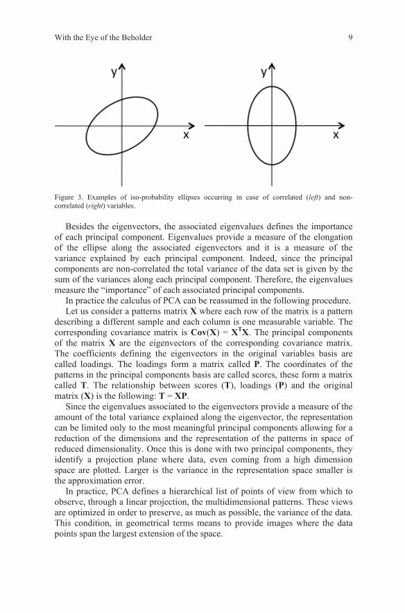
4. An example of PCA

In order to illustrate the application of PCA let us consider a number of peaches each of a different cultivar. For each peach the following quantities were measured: pH, sucrose, glucose, fructose, malic acid, and citric acid. Experimental details about the data set are found in [5]. The scope of the experiment was to study the relationship between acids and sugars in peaches. Figure 4 shows, in a color

Figure 4. Peaches data matrices displayed in a color code. Original data (left) and autoscaled data (right).

With the Eye of the Beholder

11

code, the data matrix before and after the application of autoscaling. Original data matrix is dominated by pH and sucrose whose numerical values exceed that of the other variables. Autoscaled data matrix on the contrary displays an homo-genous distribution of the variables.

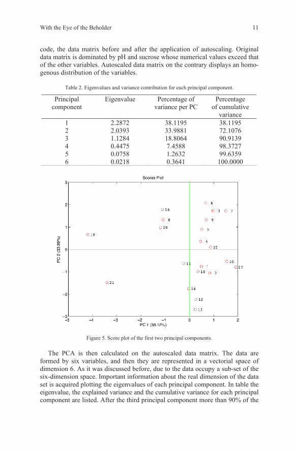
Table 2. Eigenvalues and variance contribution for each principal component.

Principal component

Eigenvalue Percentage of variance per PC

Percentage of cumulative

variance 1 2.2872 38.1195 38.1195 2 2.0393 33.9881 72.1076 3 1.1284 18.8064 90.9139 4 0.4475 7.4588 98.3727 5 0.0758 1.2632 99.6359 6 0.0218 0.3641 100.0000

Figure 5. Score plot of the first two principal components.

The PCA is then calculated on the autoscaled data matrix. The data are formed by six variables, and then they are represented in a vectorial space of dimension 6. As it was discussed before, due to the data occupy a sub-set of the six-dimension space. Important information about the real dimension of the data set is acquired plotting the eigenvalues of each principal component. In table the eigenvalue, the explained variance and the cumulative variance for each principal component are listed. After the third principal component more than 90% of the

C. Di Natale

12

total variance is explained, and the total variance is recovered with six principal components. It suggests that only a moderate correlation among the variables takes place.

Figure 5 shows the data points projected in the plane formed by the first two principal components. A plot of this kind is called scores plot. According to Table 2 the plot takes into account only 72% of the total variance of the data set. Each point of the plot corresponds to a peach whose original pattern can be seen on the matrices of Fig. 4.

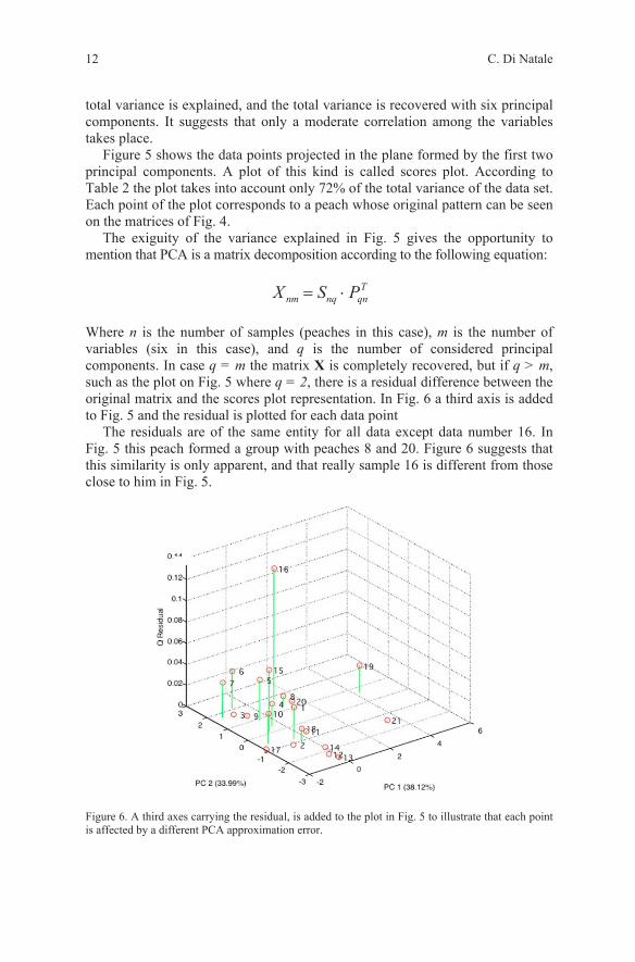
The exiguity of the variance explained in Fig. 5 gives the opportunity to mention that PCA is a matrix decomposition according to the following equation:

X nm = Snq ⋅ PqnT

Where n is the number of samples (peaches in this case), m is the number of variables (six in this case), and q is the number of considered principal components. In case q = m the matrix X is completely recovered, but if q > m, such as the plot on Fig. 5 where q = 2, there is a residual difference between the original matrix and the scores plot representation. In Fig. 6 a third axis is added to Fig. 5 and the residual is plotted for each data point

The residuals are of the same entity for all data except data number 16. In Fig. 5 this peach formed a group with peaches 8 and 20. Figure 6 suggests that this similarity is only apparent, and that really sample 16 is different from those close to him in Fig. 5.

Figure 6. A third axes carrying the residual, is added to the plot in Fig. 5 to illustrate that each point is affected by a different PCA approximation error.

With the Eye of the Beholder

13

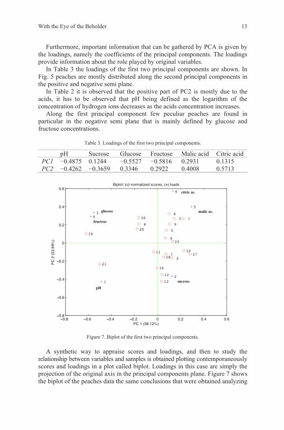
Furthermore, important information that can be gathered by PCA is given by the loadings, namely the coefficients of the principal components. The loadings provide information about the role played by original variables.

In Table 3 the loadings of the first two principal components are shown. In Fig. 5 peaches are mostly distributed along the second principal components in the positive and negative semi plane.

In Table 2 it is observed that the positive part of PC2 is mostly due to the acids, it has to be observed that pH being defined as the logarithm of the concentration of hydrogen ions decreases as the acids concentration increases.

Along the first principal component few peculiar peaches are found in particular in the negative semi plane that is mainly defined by glucose and fructose concentrations.

Table 3. Loadings of the first two principal components.

pH Sucrose Glucose Fructose Malic acid Citric acid PC1 −0.4875 0.1244 −0.5527 −0.5816 0.2931 0.1315 PC2 −0.4262 −0.3659 0.3346 0.2922 0.4008 0.5713

Figure 7. Biplot of the first two principal components.

A synthetic way to appraise scores and loadings, and then to study the relationship between variables and samples is obtained plotting contemporaneously scores and loadings in a plot called biplot. Loadings in this case are simply the projection of the original axis in the principal components plane. Figure 7 shows the biplot of the peaches data the same conclusions that were obtained analyzing

C. Di Natale

14

the table of loadings and the position of peaches data can be easily achieved looking at the biplot.

5. Caveat and conclusions

PCA is a powerful algorithm allowing for the definition of an optimal point of observation of a set of multivariate data. However, it is necessary to keep always in mind that the representation is automatically obtained maximizing the variance represented. Then it is important for a correct interpretation of the scores to evaluate the residual to appraise if some of the points are misrepresented. Nonetheless, even if residuals are moderate the score plot can still conceal important relationships among the data.

On this basis, PCA provides a simple and efficient instrument to investigate the relationship among data, and to get conclusions in phenomena even without knowledge of the processes occurring in the samples under studies. For instance, in this paper some example of alleged relationships between acids and sugars in peaches have been given without considering fruit physiology issues. Finally, it has to be remarked that statistics does not do science but it only offers either confirmation of a known law or hints to develop new knowledge, and then any conclusion we can get from data analysis has always to be scientifically justified on theoretical basis.

References

1. G. Golub, C. Van Loan, Matrix Computations, J. Hopkins University press, Baltimore, MD, 1996

2. C. Di Natale et al., Analytica Chimica Acta 459, 107–117, 2002 3. T. Jolliffe, Principal Component Analysis, Springer-Verlag, New York, 1986 4. R. Johnson, D. Wichern, Applied Multivariate Statistical Analysis, Pearson Education,

Prentice-Hall, 2002 5. M. Esti et al., in Artificial and Natural Perception: Proceedings of the 2nd Italian Conference

on Sensors and Microsystems (C. Di Natale, A. D’Amico, F. Davide, editors), World Scientific Publ. 1998

P. Malcovati et al. (eds.), Sensors and Microsystems: AISEM 2009 Proceedings, 15 Lecture Notes in Electrical Engineering 54, DOI 10.1007/978-90-481-3606-3_2, © Springer Science+Business Media B.V. 2010

BIOSENSOR TECHNOLOGY: A BRIEF HISTORY

I. PALCHETTI AND M. MASCINI Dipartimento di Chimica, Università degli Studi di Firenze, Via della Lastruccia 3,

50019 Sesto Fiorentino, Italy

1. Brief history of biosensors

The vast literature in the last 50 years related to the keyword Biosensor reveals without doubt that the scientific field is attractive. We realized at once that several researchers with different background are involved in this field of research, from chemistry to physics, to microbiologists and of course to electrical engineering, all are deeply involved in several facets of the assembly of the object “Biosensor”.

Looking at the past we realize also that the concept of Biosensor has evolved. For some authors, especially at the beginning of this research activity, i.e.

about 50 years ago, Biosensor is a self contained analytical device that responds to the concentration of chemical species in biological samples. This is clearly wrong, but it has been very difficult to clarify this point. No mention of a bio-logical active material involved in the device. Thus any physical (thermometer) or chemical sensor (microelectrode implanted in animal tissue) operating in bio-logical samples could be considered a Biosensor. We agree that a biosensor can be defined as a device that couples a biological sensing material (we can call it a molecular biological recognition element) associated with a transducer.

Recently the concept evolved again in the tentative to replace or mimic the biological material with synthetic chemical compounds.

In 1956 Professor Leland C. Clark publishes his paper on the development of an oxygen probe and based on this research activity he expanded the range of analytes that could be measured in 1962 in a Conference at a Symposium in the New York Academy of Sciences where he described how “to make electrochemical

Abstract. Biosensors use a combination of biological receptor compounds (antibody, enzyme, nucleic acid, etc.) and the physical or physic-chemical transducer directing, in most cases, “real-time” observation of a specific biological event (e.g. antibody-antigen interaction). They allow the detection of a broad spectrum of analytes in complex sample matrices, and have shown great promise in areas such as clinical diagnostics, food analysis, bio-process and environmental monitoring. Biosensors may be divided into six basic groups, depending on the method of signal transduction: optical, mass, electrochemical, magnetic, micromechanical and thermal sensors. This paper aims to give an brief tutorial of bio-sensor technology.