sesi 3 simulation basics
DESCRIPTION
NiceTRANSCRIPT
1
SIMULASI SISTEM - TKI 411 Sesi ke - 3 : Simulation Basics
Christine NataliaChristine Natalia
2
Types of Simulation
• Static or dynamics• Stochastic or deterministic• Discrete event or continuous

3
Static versus Dynamic Simulation
• A static simulation is one that is not based on time.• It often involves drawing random samples to
generate a statistical outcome, so it is sometimes called Monte Carlo simulation.
• Dynamic simulation includes the passage of time.• It looks at state changes as they occur over time.• A clock mechanism moves forward in time and state
variables are updated as time advances.
4
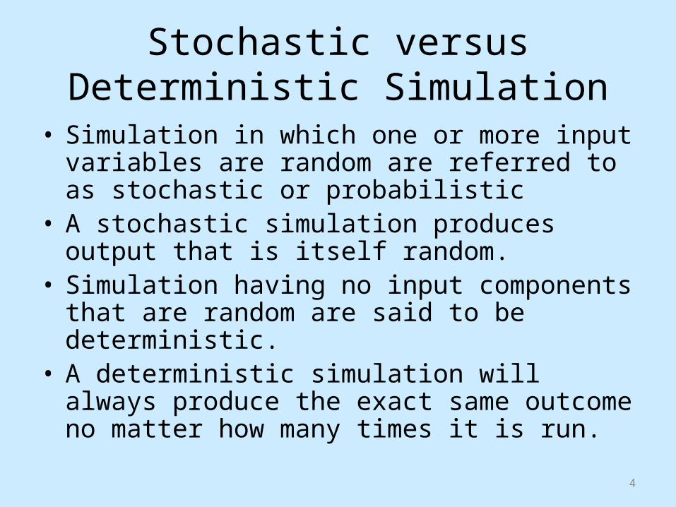
Stochastic versus Deterministic Simulation
• Simulation in which one or more input variables are random are referred to as stochastic or probabilistic
• A stochastic simulation produces output that is itself random.
• Simulation having no input components that are random are said to be deterministic.
• A deterministic simulation will always produce the exact same outcome no matter how many times it is run.

5
Stochastic versus Deterministic Simulation
• In stochastic simulation, several randomized runs or replication must be made to get an accurate estimate because each run varies statistically.
• Performance estimates for stochastic simulations are obtained by calculating the average value of performance metric across all of the replication.
6
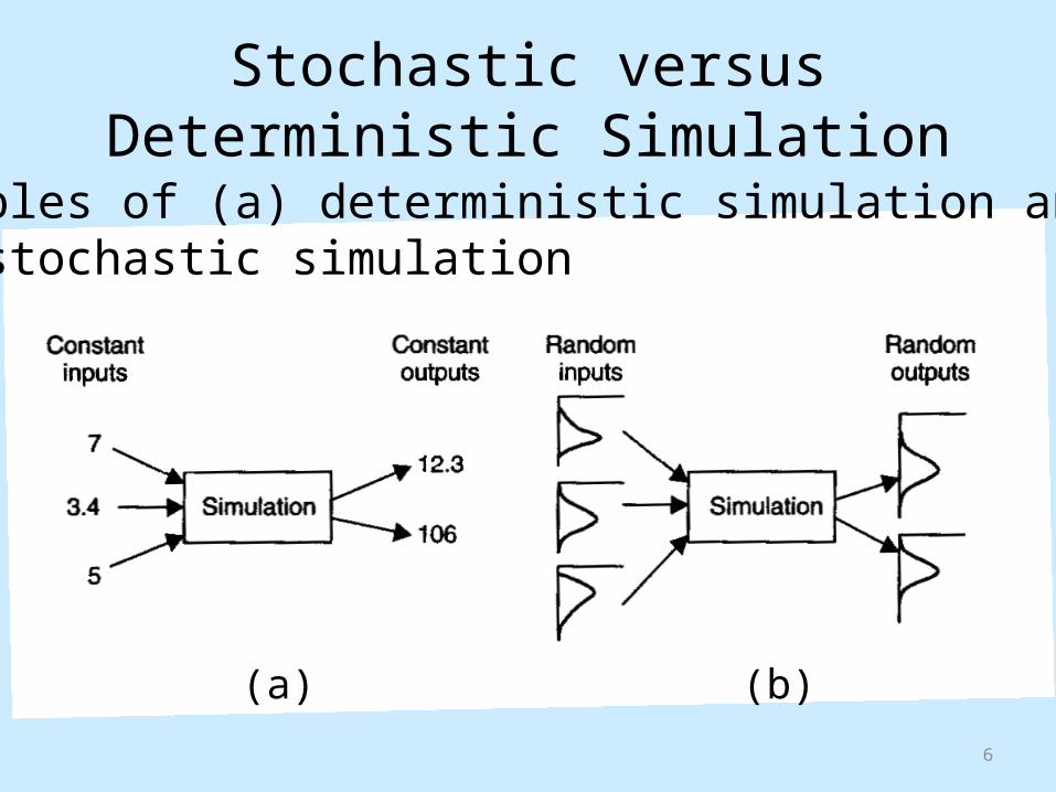
Stochastic versus Deterministic Simulation
Examples of (a) deterministic simulation and (b) stochastic simulation
(a) (b)

7
Random Behavior
• Natural behavior• Values vary within a given range and
according to a probability distribution.• Probability distributions are useful for
predicting the values, where these values are random variables.– Depend on the type of distribution and their
parameters.
8
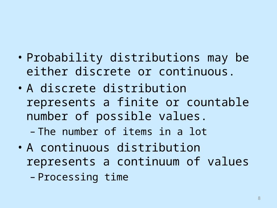
• Probability distributions may be either discrete or continuous.
• A discrete distribution represents a finite or countable number of possible values.– The number of items in a lot
• A continuous distribution represents a continuum of values– Processing time
9
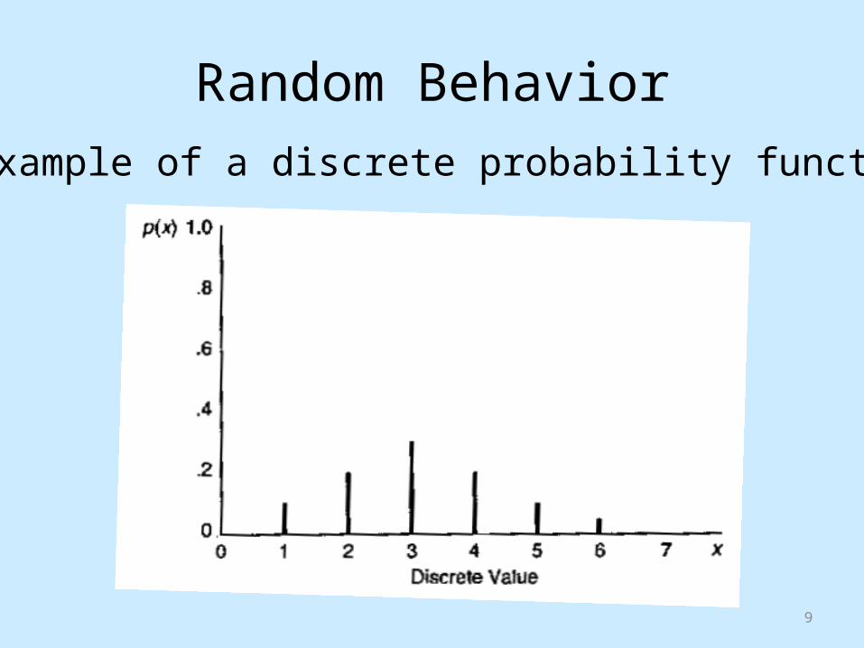
Random BehaviorAn example of a discrete probability function
10
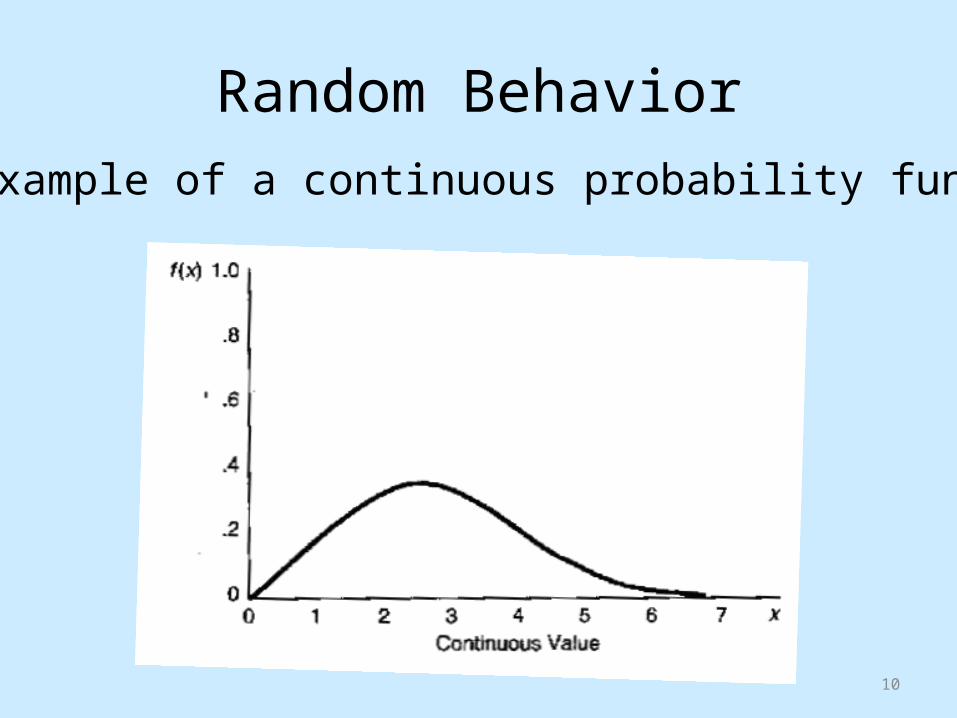
Random BehaviorAn example of a continuous probability function
11
Simulating Random Behavior
• One of the most powerful features of simulation – The ability to mimic random behavior.
• Simulating random behavior requires that a method be provided to generate random numbers as well as for generating random variates based on a given probability distribution.
12
Generating Random Numbers
• Random behavior is imitated in simulation by using a random number generator.
• Random number generator is responsible for producing this stream of independent and uniformly distributed numbers.

13
Generating Random NumbersThe U(0, 1) distribution of a randomnumber generator
14
• The numbers produced by a random number generator are not “random” in the truest sense.– The generator can produce the same sequence of
numbers again and again, which is not indicative of random behavior.
– They are often referred to as pseudo-random number generators.
• “Good” pseudo-random number generators can pump out long sequences of numbers that pass statistical tests for randomness (the numbers are independent and uniformly distributed).
15
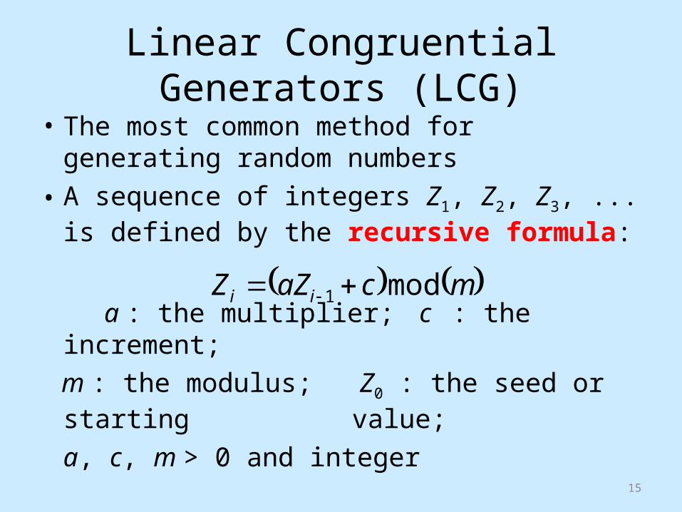
• The most common method for generating random numbers
• A sequence of integers Z1, Z2, Z3, ... is defined by the recursive formula:
a : the multiplier; c : the increment; m : the modulus; Z0 : the seed or starting
value; a, c, m > 0 and integer
mcaZZ ii mod1
Linear Congruential Generators (LCG)
16
Linear Congruential Generators (LCG).
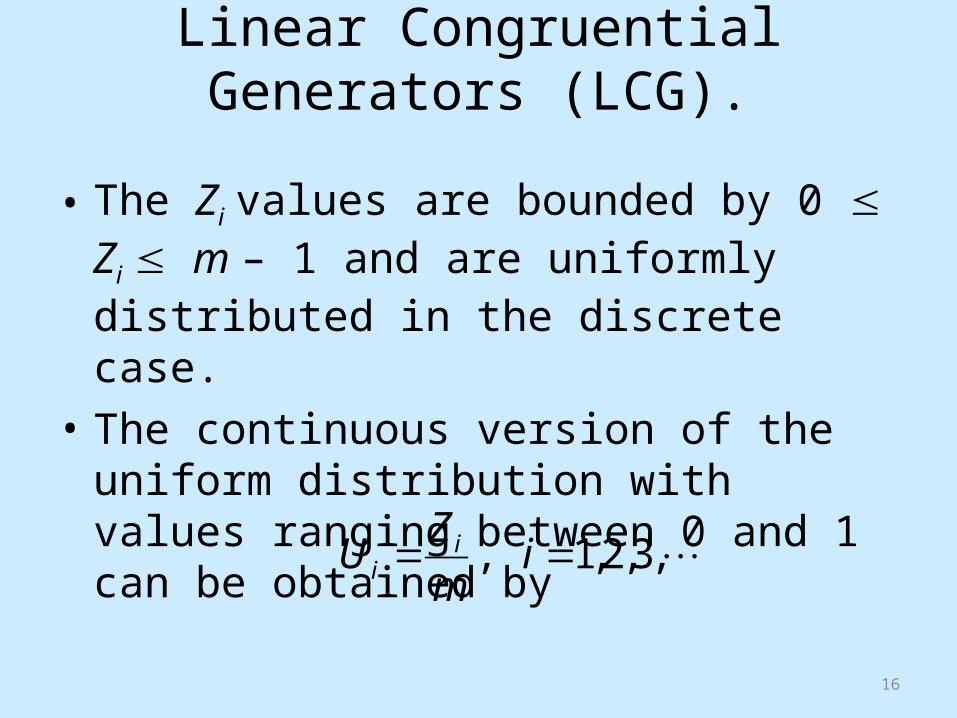
• The Zi values are bounded by 0 Zi m – 1 and are uniformly distributed in the discrete case.
• The continuous version of the uniform distribution with values ranging between 0 and 1 can be obtained by
,3,2,1 , imZU i
i

17
i Zi UiExample of LCGa = 21 0 13c = 3 1 4 0,2500m = 16 2 7 0,4375
3 6 0,37504 1 0,06255 8 0,50006 11 0,68757 10 0,62508 5 0,31259 12 0,7500
10 15 0,937511 14 0,875012 9 0,562513 0 0,000014 3 0,187515 2 0,125016 13 0,812517 4 0,250018 7 0,437519 6 0,375020 1 0,0625

18
Linear Congruential Generators (LCG).
• The maximum cycle length that an LCG can achieve is m.
• To realize maximum cycle length, the values of a, c, and m have to be carefully selected.
• A guideline for the selection is:– m = 2b where b is determined based on the number of
bits per word on the computer being used (for computer with 32 bits, b = 31)
– c and m such that their greatest common factor is 1.– a = 1 + 4k, where k is an integer.
19
• Frequently, the long sequence of random number is subdivided into smaller segments referred to as streams.
• To subdivide the generator’s sequence of random numbers into streams, it is need:– to decide how many random numbers to place in each
stream– to generate the entire sequence of random numbers
(cycle length) produced by the generator and record the Zi values that mark the beginning of each stream.
• Each stream has its own starting or seed value.
20
Linear Congruential Generators
• There are two types of LCG:– Mixed LCG– Multiplicative LCG
• Mixed LCG:– c > 0
• Multiplicative LCG– c = 0

21
Other kinds of random generators
(see Kelton pp.431-434)• More General Congruences• Composite Generators• Tauswarthe and Related Generators
22
Testing Random Number Generators
• The numbers produced by the random number generator must satisfy two properties:– Independent– Uniformly distributed between zero and one
• Generate a sequence of random numbers:U1, U2, U3, ... .

23
Testing Random Number Generators
• The hypothesis for testing the independence property:H0: Ui values from the generator are independent
H1: Ui values from the generator are not independent
• The most common statistical method the run test the runs above and below the median test the runs up and down test

24
Testing Random Number Generators
• The hypothesis for testing the uniformly property:H0: Ui values are U(0, 1)
H1: Ui values are not U(0, 1)
• The most common statistical methods: The Kolmogorov-Smirnov test The chi-square test
25
Generating Random Variates
• Methods for generating random variates (see Kelton Chap.8) Inverse transformation Composition Convolution Acceptance-Rejection Methods employing special properties
26
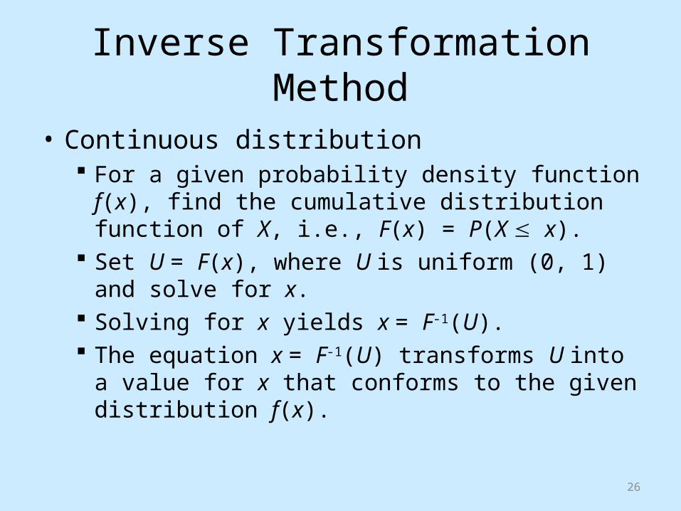
Inverse Transformation Method
• Continuous distribution For a given probability density function f(x), find
the cumulative distribution function of X, i.e., F(x) = P(X x).
Set U = F(x), where U is uniform (0, 1) and solve for x.
Solving for x yields x = F-1(U). The equation x = F-1(U) transforms U into a value
for x that conforms to the given distribution f(x).
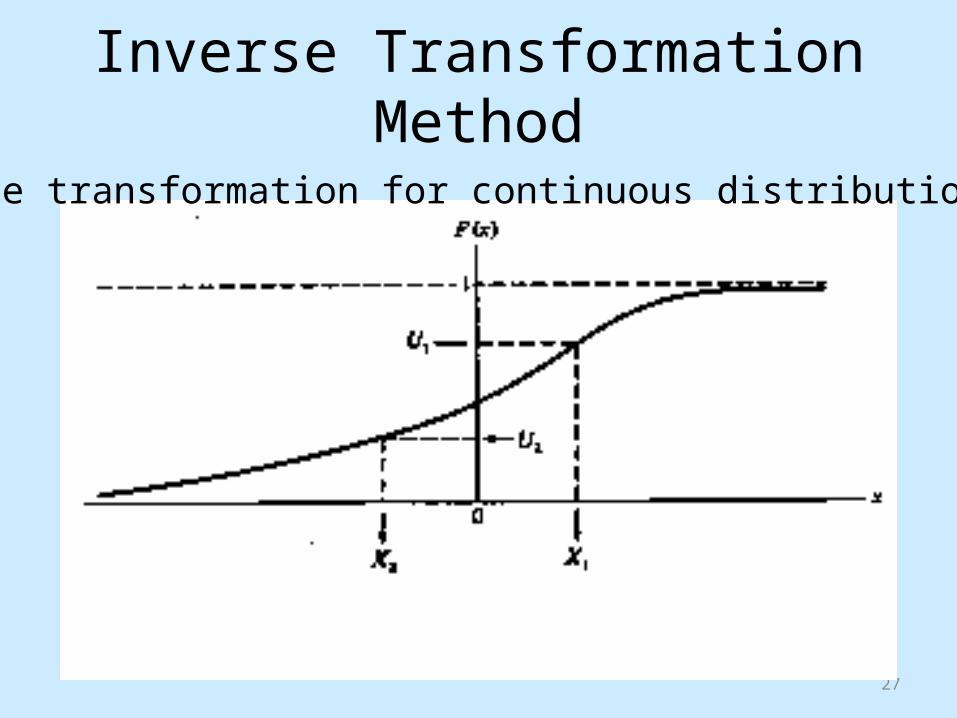
27
Inverse transformation for continuous distribution
Inverse Transformation Method
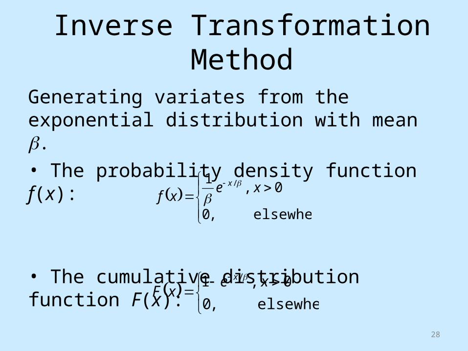
28
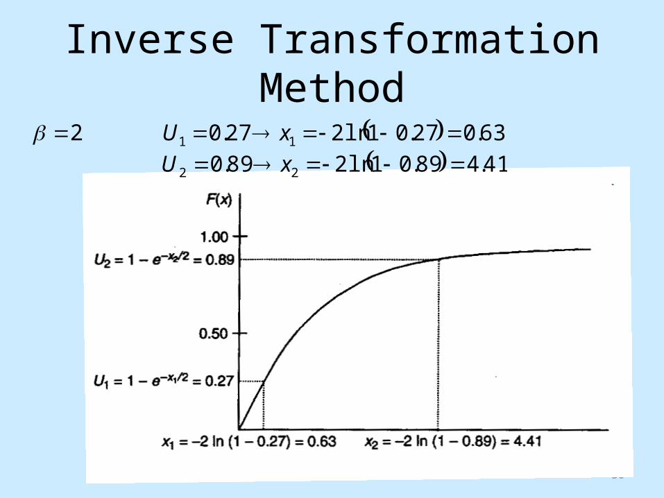
Generating variates from the exponential distribution with mean .• The probability density function f(x):
• The cumulative distribution function F(x):
elsewhere ,0
0 ,1 / xexfx
elsewhere ,00 ,1 / xe
xFx
Inverse Transformation Method
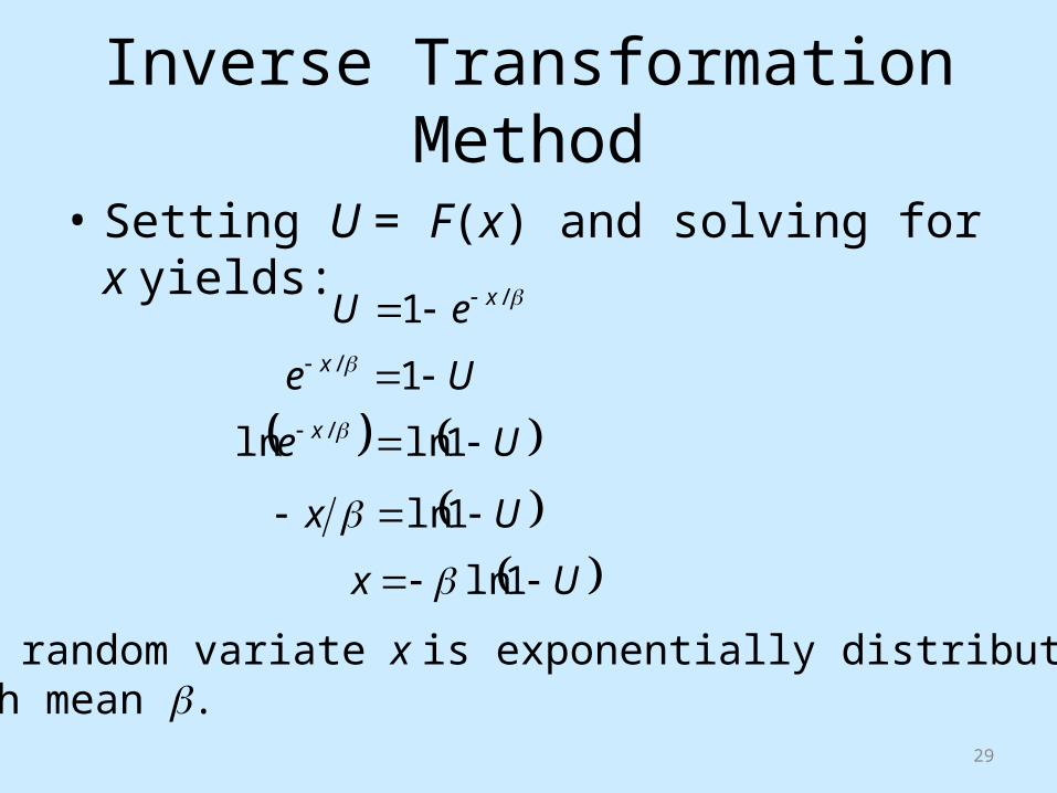
29
• Setting U = F(x) and solving for x yields:/1 xeU
Ue x 1/
Ue x 1lnln /
Ux 1ln
Ux 1ln
The random variate x is exponentially distributed with mean .
Inverse Transformation Method
30
63.027.01ln227.0 11 xU 41.489.01ln289.0 22 xU
2
Inverse Transformation Method
31
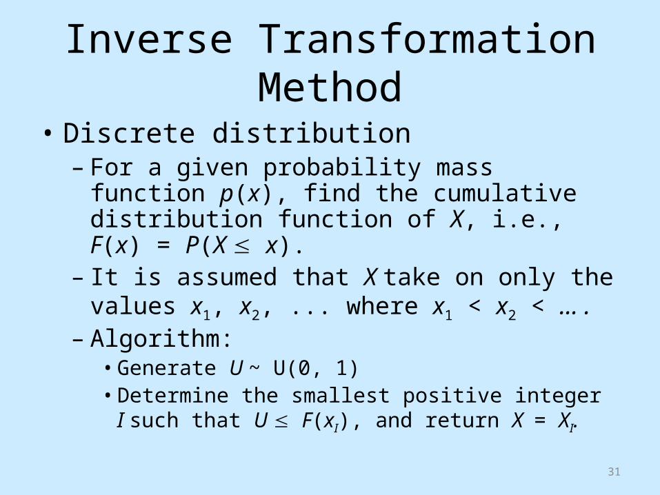
• Discrete distribution– For a given probability mass function p(x), find the
cumulative distribution function of X, i.e., F(x) = P(X x).
– It is assumed that X take on only the values x1, x2, ... where x1 < x2 < ... .
– Algorithm:• Generate U ~ U(0, 1)• Determine the smallest positive integer I such that U
F(xI), and return X = XI.
Inverse Transformation Method
32
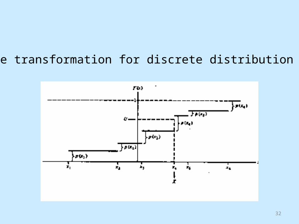
Inverse transformation for discrete distribution

33
Generating variates from the following probability mass function (arbitrary discrete distribution):
3 ,60.02 ,30.01 ,10.0
xxx
xXPxp
Inverse Transformation Method

34
The cumulative distribution function F(x)
U1 = 0.27, because 0.10 < U1 0.40 then x1 = 2

35
Generating variates from other distributions:
• Techniques and algorithms for generating variates from other distributions:– continuous: uniform, exponential, m-Erlang, Gamma,
Weibull, normal, lognormal, beta, Pearson type V, Pearson type VI, triangular, empirical distribution,
– discrete: Bernoulli, discrete uniform, arbitrary discrete distribution, binomial, geometric, negative binomial, Poisson
see Law and Kelton, Simulation Modeling and Analysis, Chapter 8.
36
Simple Speadsheet Simulation
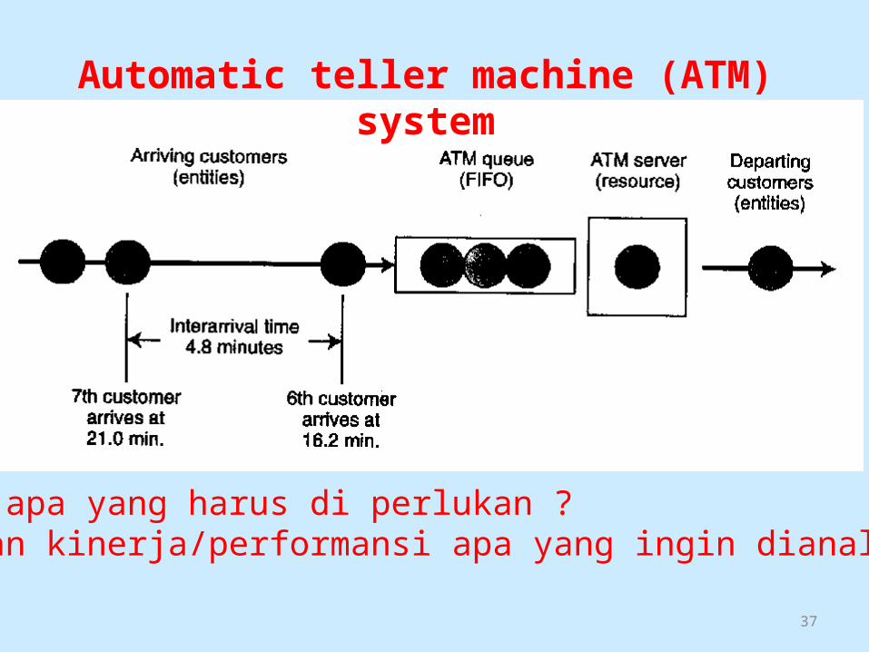
• This shows a simple spreadsheet simulation for a single-server queuing system (i.e., ATM system)– Queuing model : (M/M/1): (FIFO//)– Interarrival time ~ exponential distribution with
mean = 3.0 minutes– Service time ~ exponential distribution with mean
= 2.4 minutes.
37
Automatic teller machine (ATM) system
Data apa yang harus di perlukan ?Ukuran kinerja/performansi apa yang ingin dianalisis ?

38
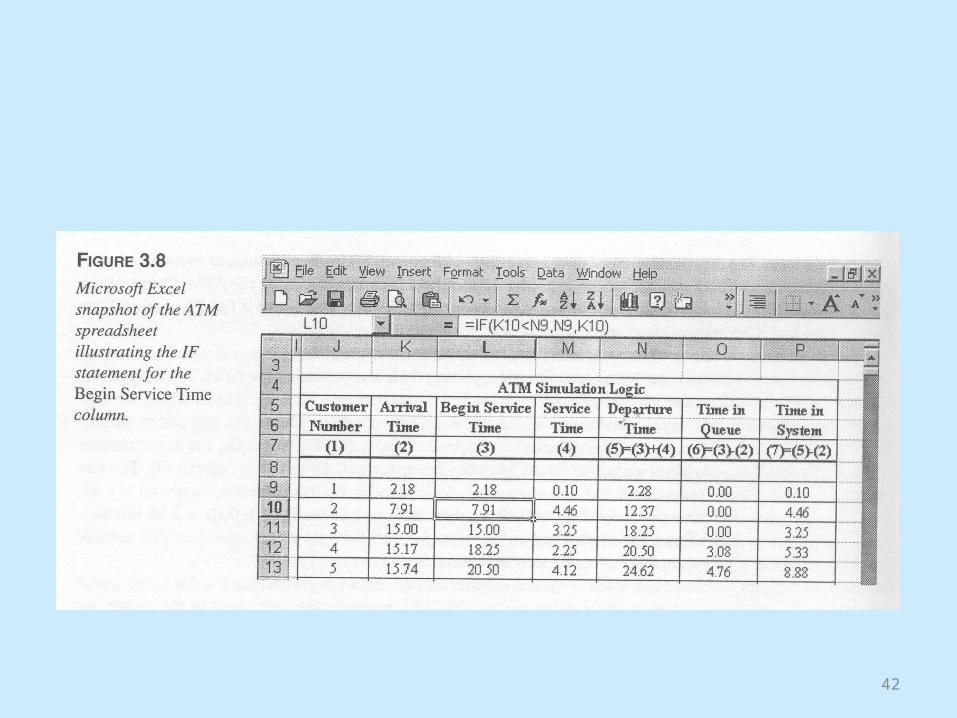
TIME CALCULATION
ArrivalTime (i) = ArrivalTime (i – 1) + InterarrivalTime (i)
If ArrivalTime (i) < DepartureTime (i – 1) then BeginServiceTime (i) = DepartureTime (i – 1)elseBeginServiceTime (i) = Arrival (i)
DepartureTime (i) = BeginServiceTime (i ) + ServiceTime (i)
TimeInQueue (i) = BeginServiceTime (i) – ArrivalTime (i)
TimeInSystem (i) = DepartureTime (i) – ArrivalTime (i)
39
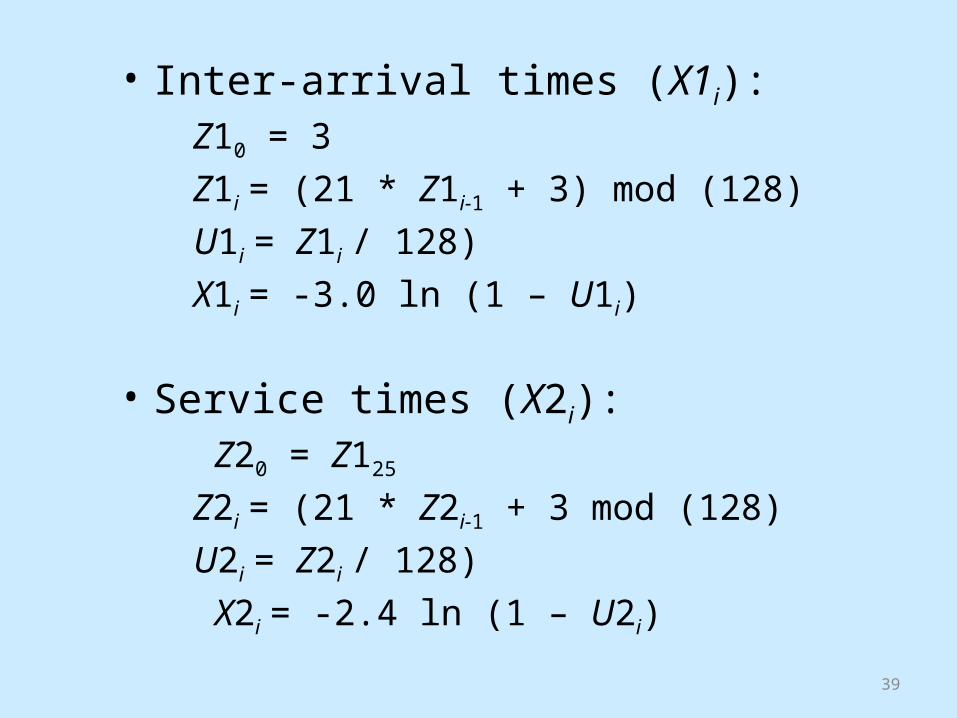
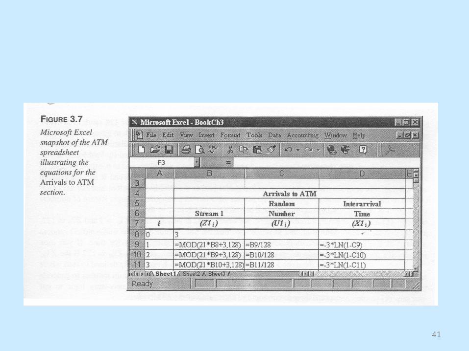
• Inter-arrival times (X1i):Z10 = 3Z1i = (21 * Z1i-1 + 3) mod (128)U1i = Z1i / 128)X1i = -3.0 ln (1 – U1i)
• Service times (X2i): Z20 = Z125
Z2i = (21 * Z2i-1 + 3 mod (128)U2i = Z2i / 128) X2i = -2.4 ln (1 – U2i)

40
i Stream 1 Random Interarrival Steam 2 Random Service Customer Arrival Begin Service Service Departure Time in Time inNumber Time Number Time Number Time Time Time Time Queue System
0 3 1221 66 0,516 2,17 5 0,039 0,10 1 2,17 2,17 0,10 2,27 0,00 0,102 109 0,852 5,72 108 0,844 4,46 2 7,90 7,90 4,46 12,35 0,00 4,463 116 0,906 7,10 95 0,742 3,25 3 15,00 15,00 3,25 18,25 0,00 3,254 7 0,055 0,17 78 0,609 2,26 4 15,17 18,25 2,26 20,51 3,08 5,345 22 0,172 0,57 105 0,820 4,12 5 15,73 20,51 4,12 24,63 4,77 8,896 81 0,633 3,01 32 0,250 0,69 6 18,74 24,63 0,69 25,32 5,89 6,587 40 0,313 1,12 35 0,273 0,77 7 19,86 25,32 0,77 26,08 5,46 6,228 75 0,586 2,65 98 0,766 3,48 8 22,51 26,08 3,48 29,57 3,58 7,069 42 0,328 1,19 13 0,102 0,26 9 23,70 29,57 0,26 29,82 5,87 6,12
10 117 0,914 7,36 20 0,156 0,41 10 31,06 31,06 0,41 31,47 0,00 0,4111 28 0,219 0,74 39 0,305 0,87 11 31,80 31,80 0,87 32,68 0,00 0,8712 79 0,617 2,88 54 0,422 1,32 12 34,68 34,68 1,32 36,00 0,00 1,3213 126 0,984 12,48 113 0,883 5,15 13 47,16 47,16 5,15 52,31 0,00 5,1514 89 0,695 3,57 72 0,563 1,98 14 50,73 52,31 1,98 54,29 1,58 3,5615 80 0,625 2,94 107 0,836 4,34 15 53,67 54,29 4,34 58,63 0,62 4,9616 19 0,148 0,48 74 0,578 2,07 16 54,15 58,63 2,07 60,70 4,48 6,5517 18 0,141 0,45 21 0,164 0,43 17 54,61 60,70 0,43 61,13 6,09 6,5218 125 0,977 11,26 60 0,469 1,52 18 65,87 65,87 1,52 67,38 0,00 1,5219 68 0,531 2,27 111 0,867 4,85 19 68,14 68,14 4,85 72,98 0,00 4,8520 23 0,180 0,59 30 0,234 0,64 20 68,73 72,98 0,64 73,63 4,25 4,8921 102 0,797 4,78 121 0,945 6,97 21 73,52 73,63 6,97 80,60 0,11 7,0822 97 0,758 4,25 112 0,875 4,99 22 77,77 80,60 4,99 85,59 2,83 7,8223 120 0,938 8,32 51 0,398 1,22 23 86,09 86,09 1,22 87,31 0,00 1,2224 91 0,711 3,72 50 0,391 1,19 24 89,81 89,81 1,19 91,00 0,00 1,1925 122 0,953 9,18 29 0,227 0,62 25 98,99 98,99 0,62 99,61 0,00 0,62
Average 1,94 4,26
Arrival to ATM ATM Processing Time ATM Simulation Logic
41
42

43
Simulation Replications and Output Analysis
• The spreadsheet simulation of the first 25 customers to arrive to the ATM system
• The simulation output gives:– average time in queue = 1.94 minute– average time in system = 4.26 minute
• These results represent only one possible value of each performance measure.
• If at least one input variable to the simulation model is random, then the output of the simulation model will also be random.
44
• The inter-arrival times of customers and their service times are random variables, then the output of the simulation model is also random.
• The 2nd replication change the seed valuesZ10 = 29
Z20 = Z125 = 92
45
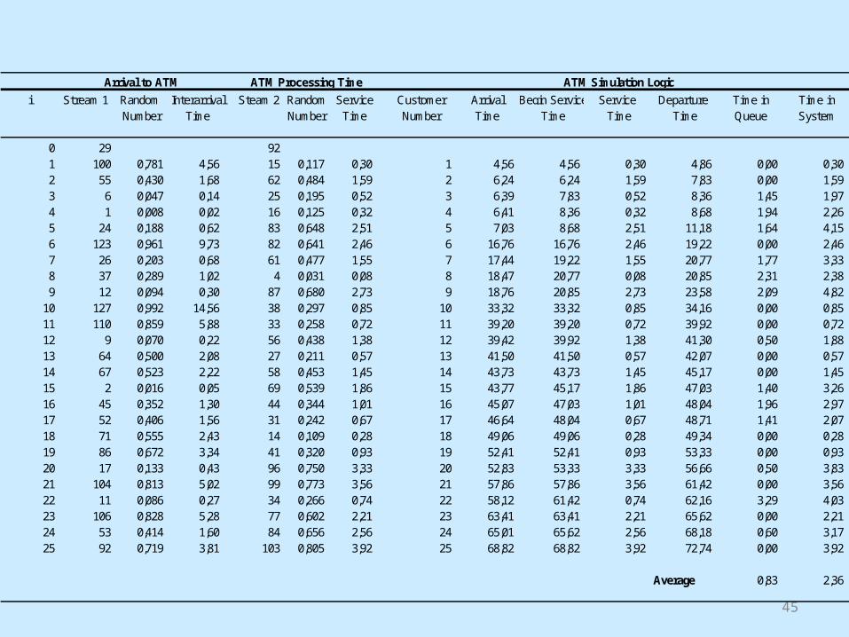
i Stream 1 Random Interarrival Steam 2 Random Service Customer Arrival Begin Service Service Departure Time in Time inNumber Time Number Time Number Time Time Time Time Queue System
0 29 921 100 0,781 4,56 15 0,117 0,30 1 4,56 4,56 0,30 4,86 0,00 0,302 55 0,430 1,68 62 0,484 1,59 2 6,24 6,24 1,59 7,83 0,00 1,593 6 0,047 0,14 25 0,195 0,52 3 6,39 7,83 0,52 8,36 1,45 1,974 1 0,008 0,02 16 0,125 0,32 4 6,41 8,36 0,32 8,68 1,94 2,265 24 0,188 0,62 83 0,648 2,51 5 7,03 8,68 2,51 11,18 1,64 4,156 123 0,961 9,73 82 0,641 2,46 6 16,76 16,76 2,46 19,22 0,00 2,467 26 0,203 0,68 61 0,477 1,55 7 17,44 19,22 1,55 20,77 1,77 3,338 37 0,289 1,02 4 0,031 0,08 8 18,47 20,77 0,08 20,85 2,31 2,389 12 0,094 0,30 87 0,680 2,73 9 18,76 20,85 2,73 23,58 2,09 4,82
10 127 0,992 14,56 38 0,297 0,85 10 33,32 33,32 0,85 34,16 0,00 0,8511 110 0,859 5,88 33 0,258 0,72 11 39,20 39,20 0,72 39,92 0,00 0,7212 9 0,070 0,22 56 0,438 1,38 12 39,42 39,92 1,38 41,30 0,50 1,8813 64 0,500 2,08 27 0,211 0,57 13 41,50 41,50 0,57 42,07 0,00 0,5714 67 0,523 2,22 58 0,453 1,45 14 43,73 43,73 1,45 45,17 0,00 1,4515 2 0,016 0,05 69 0,539 1,86 15 43,77 45,17 1,86 47,03 1,40 3,2616 45 0,352 1,30 44 0,344 1,01 16 45,07 47,03 1,01 48,04 1,96 2,9717 52 0,406 1,56 31 0,242 0,67 17 46,64 48,04 0,67 48,71 1,41 2,0718 71 0,555 2,43 14 0,109 0,28 18 49,06 49,06 0,28 49,34 0,00 0,2819 86 0,672 3,34 41 0,320 0,93 19 52,41 52,41 0,93 53,33 0,00 0,9320 17 0,133 0,43 96 0,750 3,33 20 52,83 53,33 3,33 56,66 0,50 3,8321 104 0,813 5,02 99 0,773 3,56 21 57,86 57,86 3,56 61,42 0,00 3,5622 11 0,086 0,27 34 0,266 0,74 22 58,12 61,42 0,74 62,16 3,29 4,0323 106 0,828 5,28 77 0,602 2,21 23 63,41 63,41 2,21 65,62 0,00 2,2124 53 0,414 1,60 84 0,656 2,56 24 65,01 65,62 2,56 68,18 0,60 3,1725 92 0,719 3,81 103 0,805 3,92 25 68,82 68,82 3,92 72,74 0,00 3,92
Average 0,83 2,36
Arrival to ATM ATM Processing Time ATM Simulation Logic
46
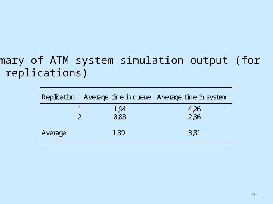
Replication Average time in queue Average time in system1 1,94 4,262 0,83 2,36
Average 1,39 3,31
Summary of ATM system simulation output (for two replications)
47
Generating Random Variates

48
Uniform
• Generate U ~ U(0,1)1. Return X = a + (b – a)U

49
Uniform
• The distribution function of a U(a, b) random variable is easily inverted by solving u = F(x) for x to obtain, for 0 u 1,
• Algorithm:1. Generate U ~ U(0, 1)2. Return X = a + (b – a)U
50
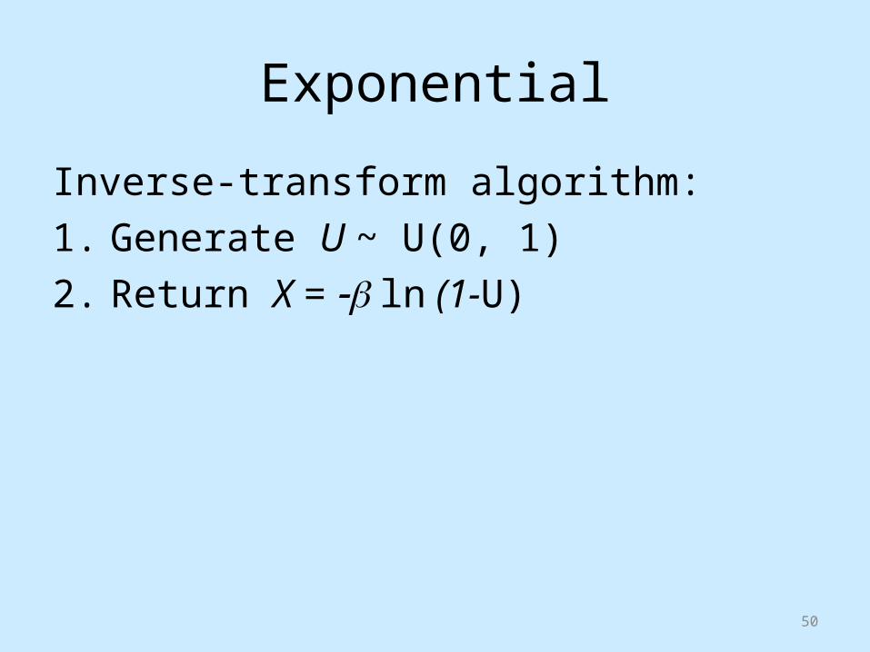
Exponential
Inverse-transform algorithm:1. Generate U ~ U(0, 1)2. Return X = ln (1-U)

51
m-Erlang
• If X is an m-Erlang random variable with mean , it can be written X = Y1 + Y2 + ... + Ym, where Yi’s are IID exponential random variable, each with mean /m.
• Algorithm:1. Generate U1, U2, ..., Um as IID U(0, 1)
2. Return
m
iiU
mX
1
ln
52
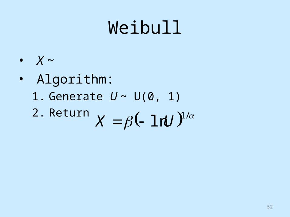
Weibull
• X ~ • Algorithm:
1. Generate U ~ U(0, 1)2. Return /1lnUX
53
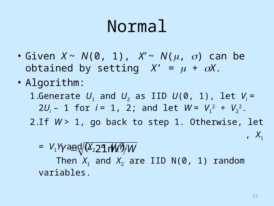
Normal
• Given X ~ N(0, 1), X’ ~ N(, ) can be obtained by setting X’ = + X.
• Algorithm:1. Generate U1 and U2 as IID U(0, 1), let Vi = 2Ui – 1
for i = 1, 2; and let W = V12 + V2
2.
2. If W > 1, go back to step 1. Otherwise, let , X1 = V1Y and X2 = V2Y.
Then X1 and X2 are IID N(0, 1) random variables.
WWY ln2

54
Lognormal
If Y ~ N(, 2) then eY ~ LN(, 2).Algorithm:1. Generate Y ~ N(, 2).2. Return X ~ eY.

55
Beta

56
Generating Discrete Random Variates
• Bernoulli• Discrete uniform• Binomial• Geometric• Negative binomial• Poisson

57
Binomial
Algorithm:1. Generate Y1, Y2, ..., Yt as IID Bernoulli(p)
random variates.2. Return X = Y1 + Y2 + ...,+ Yt
58
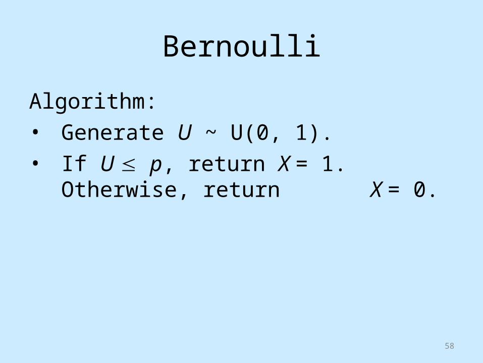
Bernoulli
Algorithm:• Generate U ~ U(0, 1).• If U p, return X = 1. Otherwise, return X
= 0.
59
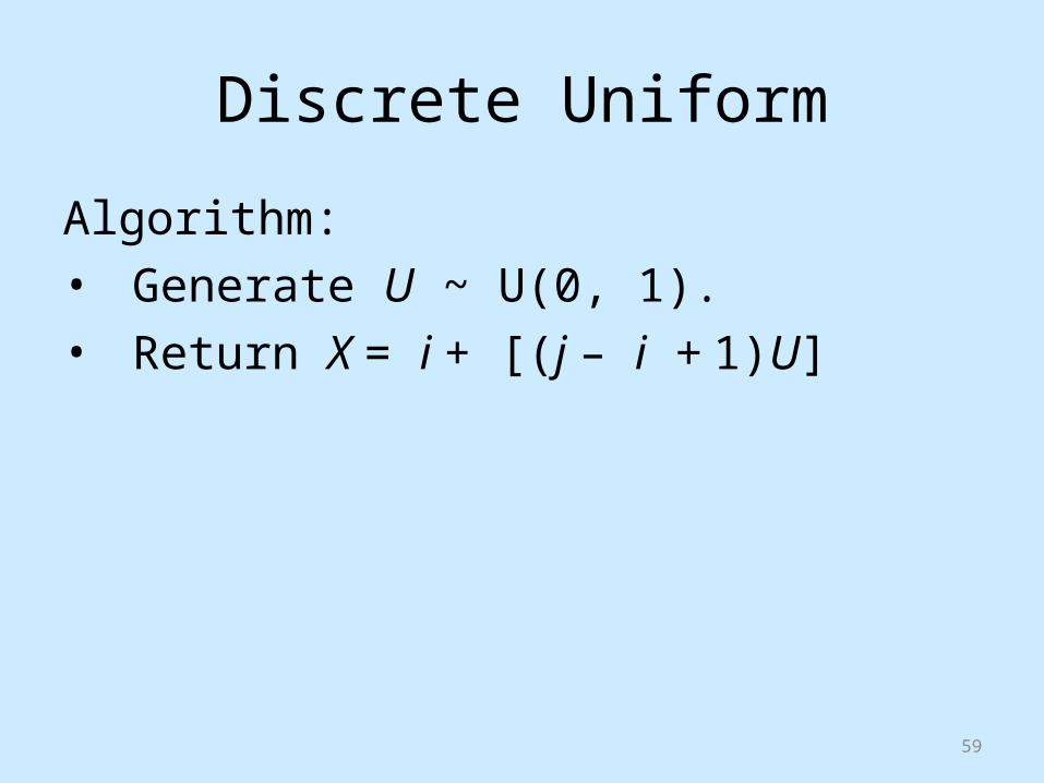
Discrete Uniform
Algorithm:• Generate U ~ U(0, 1).• Return X = i + [(j – i + 1)U]
60
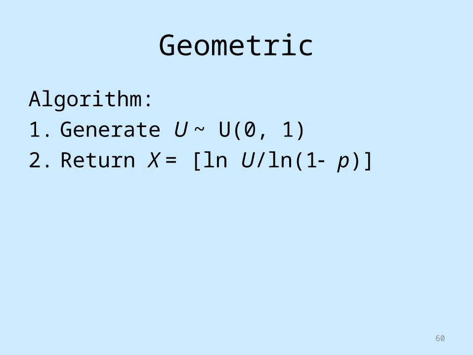
Geometric
Algorithm:1. Generate U ~ U(0, 1)2. Return X = [ln U/ln(1 p)]

61
Negative Binomial
Algorithm:1. Generate Y1, Y2, ..., Ys as IID geom(p) random
variates.2. Return X = Y1 + Y2 + ...,+ Ys

62
Poisson
Algorithm:1. Let a = e, b = 1, and i = 0.2. Generate Ui+1 ~ U(0, 1) and replace b by
bUi+1. If b < a, return X = i. Otherwise, go to step 3.
3. Replace i by i + 1 and go back step 2.