Shift-Map Image Editing

Yael Pritch Eitam Kav-Venaki Shmuel Peleg

School of Computer Science and EngineeringThe Hebrew University of Jerusalem

91904 Jerusalem, Israel

Abstract

Geometric rearrangement of images includes operationssuch as image retargeting, inpainting, or object rearrange-ment. Each such operation can be characterized by a shift-map: the relative shift of every pixel in the output imagefrom its source in an input image.

We describe a new representation of these operations asan optimal graph labeling, where the shift-map representsthe selected label for each output pixel. Two terms are usedin computing the optimal shift-map: (i) A data term whichindicates constraints such as the change in image size, ob-ject rearrangement, a possible saliency map, etc. (ii) Asmoothness term, minimizing the new discontinuities in theoutput image caused by discontinuities in the shift-map.

This graph labeling problem can be solved using graphcuts. Since the optimization is global and discrete, it out-performs state of the art methods in most cases. Efficienthierarchical solutions for graph-cuts are presented, and op-erations on 1M images can take only a few seconds.

1. Introduction

Geometric image rearrangement is becoming more pop-ular as it is being enabled by recent computer vision tech-nologies. While early manipulations included mostly cropand scale, modern tools enable smart photomontage [1], im-age resizing (a.k.a. “retargeting”) [2, 13, 19, 14, 16], ob-ject rearrangement and removal [5, 14, 6]. Recent retarget-ing methods propose effective resizing by examining imagecontent and removing “less important” regions. Fig. 1 andFig. 2 show comparisons of a few retargeting methods.

Seam carving [2, 13] performs retargeting by iterativeremoval of narrow curves from the image. As an iterativegreedy algorithm no global optimization can be made, andsomething as simple as removing one of several similar ob-jects is impossible. Since seam carving removes regionshaving low gradients, significant distortions occur whenmost image regions have many gradients.

a)

b) c)

d) e)Figure 1. Comparison of a few retargeting methods, reducingwidth by half. (a) Original image. (b) Video-retargeting [19];(c) Optimized scale-and-stretch [16]; (d) Improved Seam Carving[13]; (e) Our shift-map editing.

The use of a continuous image warping for retargetingwas proposed in [19, 16]. While providing global con-siderations, continuous warping can introduce significantdistortions, and good object removal is almost impossible.Both methods use saliency maps (e.g. face detection), and

151 2009 IEEE 12th International Conference on Computer Vision (ICCV) 978-1-4244-4419-9/09/$25.00 ©2009 IEEE

a) b)

c) d) e)Figure 2. Comparison of a few retargeting methods, reducingwidth by half. (a) Original image. (b) Our shift-map editing.(c) Video-retargeting [19]; (d) Optimized scale-and-stretch [16];(e) Improved Seam Carving [13];

saliency mistakes cause distorted results. One of the ma-jor problems in these methods is the application of differentscaling to different objects. This causes most of the distor-tions visible in Fig. 1.(b-c).

An approach based on bidirectional similarity is pre-sented in [14], which also names retargeting as “summa-rization”. Every feature in the input should appear in theoutput, and every feature in the output should appear in theinput. This method can also be used for image rearrange-ment.

The method most related to our work is the patch trans-form [5], which segments the image into patches which arethan rearranged using global optimization. The need forprior determination of the patch size is a major drawbackof this method. Also, the patches reduce significantly theflexibility for rearrangement and composition. The inherentproblems of using patches are also affecting the object re-moval in [9]. We found that our results, moving individualpixels, significantly improve the results in [5].

In shift-map editing a global optimization for a discretelabeling is performed over individual pixels, overcomingmost of the difficulties of previous methods. This is demon-strated in the simple retargeting example in Fig. 2, wherebest retargeting is very easy: a simple removal of a segmentin the net that leaves its structure intact. This is easily possi-ble with shift-map. In general, shift-map avoids scaling andmostly remove or shift image regions. Multi resolution op-timization makes the shift-map computation very efficient,and most of the examples in this paper were prepared in lessthan 30 seconds.

2. Image Editing as Graph Labeling

The relationship between an input image I(x, y) and anoutput image R(u, v) in image rearrangement and retarget-ing is defined by a shift-map M(u, v) = (tx, ty). Theoutput pixel R(u, v) will be derived from the input pixelI(u + tx, v + ty).

The optimal shift-map is defined as a graph labeling,where the nodes are the pixels of the output image, and eachoutput pixel can be labeled by a shift (tx, ty). The optimalshift-map M minimizes the following cost function:

E(M) = α∑p∈R

Ed(M(p)) +∑

(p,q)∈N

Es(M(p), M(q)), (1)

where Ed is a data term providing external requirements,and Es is a smoothness term defined over neighboring pix-els N . α is a user defined weight balancing the two terms,and in all our examples we used α = 1. Each term will nowbe defined in detail. Once the graph is given, the shift-maplabeling is computed using multi-label graph cuts [8, 4, 3].

2.1. Single Pixel Data Term

The data term Ed is used to enter external constraints.We will describe the cases of pixel rearrangement, pixel re-moval, and pixel saliency.

2.1.1 Pixel Rearrangement

When an output pixel (u, v) should originate from location(x, y) in the input image, the appropriate shift gets zero en-ergy while all other shifts get a very high energy. This isexpressed in the following equation:

Ed(M(u, v)) =

{(u + tx = x) ∧ (v + ty = y) 0otherwise ∞ (2)

For example, in changing the width of the image, thisconstraint is used to determine that both the leftmost andrightmost columns of the output image will come from theleftmost and rightmost columns of the input image.

2.1.2 Pixel Saliency and Removal

Specific pixels in the input image can be forced to appearor to disappear in the output image. A saliency map S(x, y)will be very high for pixels to be removed, and very low forsalient pixels that should not be removed. The data term Ed

for an output pixel (u, v) with a shift-map (tx, ty) will be

Ed(M(u, v)) = S(u + tx, v + ty) (3)

It is also possible to use automatic saliency map com-puted from the image such as the ones proposed in [19, 16].

152

2.2. Smoothness Term for Pixel Pairs

The smoothness term Es(M(p), M(q)) represents dis-continuities added to the output image by discontinuitiesin the shift-map. A shift-map discontinuity exists betweentwo neighboring locations (u1, v1) and (u2, v2) in the out-put image R if their shift-maps are different: M(u1, v1) �=M(u2, v2). The smoothness term Es(M) takes into ac-count both color differences and gradient differences be-tween corresponding spatial neighbors in the output imageand in the input image to create good stitching. This treat-ment is similar to [1].

Es(M) = (4)∑(u,v)∈R

∑i

(R((u, v) + ei)− I((u, v) + M(u, v) + ei))2+

β∑

(u,v)∈R

∑i

(�R((u, v)+ei)−�I((u, v)+M(u, v)+ei))2,

where ei are the four unit vectors representing the fourspatial neighbors of a pixel, the color differences are Eu-clidean distances in RGB, �I and �R are the magnitudeof the image gradients at these locations, and β is a weightto combine these two terms. In most of our experiments weused β = 2. As both color differences and gradient differ-ences are used for smoothness, structure is better preserved.

As we use non metric distances, many of the theoreticalguarantees of the alpha expansion algorithm are lost. How-ever, in practice we have found that good results are ob-tained. We further found that squaring the differences gavebetter results than using the absolute value, preferring manysmall stitches over one large jump. Deviation from a metricdistance was also made in [10, 1].

3. Hierarchical Solution for Graph Labeling

Finding the optimal graph labeling as described in theprevious section can be computationally infeasible, due tothe very large number of nodes and of labels. In some casesa pixel in the output image could originate from any pixelin the input image and the number of possible labels is thenumber of pixels in the input image.

A heuristic hierarchical approach for finding the opti-mal graph labeling can substantially reduces the memoryand computational requirements of the graph-cut algorithm.It provides good results for most of the shift map editingapplications, even though optimality cannot be guaranteed.The speedup obtained by this approach is of several ordersof magnitude, turning an intractable problem into a problemthat can be solved in a few seconds.

A full shift map is first solved in a coarse resolution,in which both the number of nodes (image pixels) and thenumber of labels (possible shifts) are reduced. For exam-ple, at the 4th pyramid level the number of nodes and the

(a) (b)

(c) (d) (e)Figure 3. Shift-map retargeting for different output widths. In eachcase different objects are removed. (a) Original image taken from[13]; (b-c-e) Different output widths using no saliency. (d) Samewidth as (c), but the child was marked salient.

number of labels are reduced by a factor of 64 (in the case ofboth horizontal and vertical shifts). Once a coarse shift-mapis found, it is interpolated to an initial guess for a higher res-olution using a nearest neighbor interpolation, and the shift-map values are doubled to match the higher image resolu-tion.

In the higher resolution levels only small shifts relativeto the initial guess are examined. In our implementation,we used three relative shifts, (-1, 0, +1), in each coordinate,giving a total of nine labels for both directions. It is impor-tant to note that the data and smoothness terms are alwayscomputed with respect to the actual shifts, and not to thelabels. We used three to five pyramid levels, such that thecoarsest level contains up to 100 × 100 pixels. The shiftmap computation took between 0.5 to 30 seconds for mostof the examples in this paper. To increase accuracy in la-bel discontinuities, more than three refinement labels can beused. For example, the possible labels of a pixel can repre-sent not only shifts from its own parent, but also shifts fromthe neighbors of its parent. This will improve accuracy atshift discontinuities, but at higher computational and mem-ory costs.

While the hierarchical approach is not guaranteed to givethe global optimum, the results are very good as can be seenin the examples. It is likely that this success, as the successof most pyramid approaches in computer vision, can be at-tributed to the observation that a natural image includes in-formation in all frequencies. A multi-resolution method forgraph-cuts with two labels (min-cut) was used in [11, 13],and was shown to provide good results. The contribution inthis paper is to extend this case to multiple labels depictingimage displacement.

153

4. Shift-Map Applications

Shift-map is computed by an optimal graph labeling,where a node in the graph corresponds to a pixel in the out-put image. In the section we describe how to build the graphand use shift-maps for several image editing applications.

4.1. Image Retargeting

Image retargeting is the change of image size, which istypically done in only a single direction in order to changethe image aspect ratio. We will assume that the change isin image width, but we could also address changing bothimage dimensions.

4.1.1 Label Order Constraint

In image resizing it is reasonable to assume that the shift-map will retain the spatial order of objects, and the left-right relationship will not be inverted. This implies a mono-tonic shift-map. In the case of reducing image width, ifM(u, v) = (tx, ty) and M(u + 1, v) = (t′x, t′y), thant′x ≥ tx. This restriction limits the number of possible la-bels to be the number of removed pixels: when reducing orincreasing the width of the input image by 100 pixels, thelabel of each pixel can only be one of 101 labels. In addi-tion, the smoothness term will give an infinite cost to caseswhen t′x < tx. Note that for reducing image width the val-ues of tx are non negative, and for increasing image widththe values of tx are non positive and t′x ≤ tx. The orderconstraint is important also in case a saliency map is used,as it helps to avoid duplication of salient pixels.

Theoretically, only horizontal shifts need to be consid-ered for horizontal resizing. However, this makes it im-possible to respect geometrical image properties such asstraight diagonal lines. When small vertical shifts are al-lowed, in addition to the horizontal shifts, the smoothnessterm will better preserve image structure.

4.1.2 Controlling Object Removal

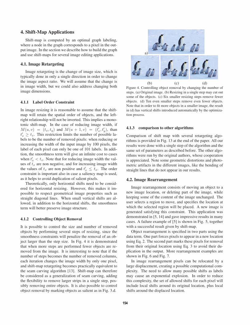
It is possible to control the size and number of removedobjects by performing several steps of resizing, since thesmoothness constraints will penalize the removal of an ob-ject larger than the step size. In Fig. 4 it is demonstratedthat when more steps are performed fewer objects are re-moved from the image. It is interesting to note that if thenumber of steps becomes the number of removed columns,each iteration changes the image width by only one pixel,and shift-map retargeting becomes practically equivalent tothe seam carving algorithm [13]. Shift-map can thereforebe considered as a generalization of seam carving, addingthe flexibility to remove larger strips in a single step, pos-sibly removing entire objects. It is also possible to controlobject removal by marking objects as salient as in Fig. 3.d.

a)

(b) (c) (d)Figure 4. Controlling object removal by changing the number ofsteps. (a) Original image. (b) Resizing in a single step may cut outsome of the objects. (c) Six smaller resizing steps remove fewerobjects. (d) Ten even smaller steps remove even fewer objects.Note that in order to fit more objects in a smaller image, the resultin (d) has vertical shifts introduced automatically by the optimiza-tion process.

4.1.3 comparison to other algorithms

Comparison of shift map with several retargeting algo-rithms is provided in Fig. 13 at the end of the paper. All ourresults were done with a single step of the algorithm and thesame set of parameters as described before. The other algo-rithms were run by the original authors, whose cooperationis appreciated. Note some geometric distortions and photo-metric artifacts in the different images, like the bending ofstraight lines that do not appear in our results.

4.2. Image Rearrangement

Image rearrangement consists of moving an object to anew image location, or deleting part of the image, whilekeeping some of the content of the image unchanged. Theuser selects a region to move, and specifies the location atwhich the selected region will be placed. A new image isgenerated satisfying this constraint. This application wasdemonstrated in [5, 14] and gave impressive results in manycases. A failure example of [5] is shown in Fig. 5, togetherwith a successful result given by shift-map.

Object rearrangement is specified in two parts using thedata term. One part forces pixels to appear in a new locationusing Eq. 2. The second part marks these pixels for removalfrom their original location using Eq. 3 to avoid their du-plication in the output. More rearrangement examples areshown in Fig. 6 and Fig. 7.

In image rearrangement pixels can be relocated by alarge displacement, creating a possible computational com-plexity. The need to allow many possible shifts as labelsmay cause an exponential explosion. In order to reducethis complexity, the set of allowed shifts for each pixel willinclude local shifts around its original location, plus localshifts around the displaced location.

154

(a)

(b) (c)Figure 5. Image Rearrangement: Comparison of shift-map andpatch transform, on a failure case of the patch transform [5]. (a)The original image. (b) The user constraints marked by squareson top of the result given by patch transform: “move the personand a part of the temple to the right, and keep the tourists at theiroriginal location in the left bottom corner”. (c) Shift-map resulton the same input.

As the number of labels is growing significantly whenthere are multiple user constraints, A smart ordering isused for the alpha expansion algorithm of the graph cut [4]to enable fast convergence. The main idea of the alpha-expansion algorithm is to split the graph labels to α andnon-α, and perform a min cut between those labels allow-ing non-α labels to change to α. The algorithm will iteratethrough each possible label for α until convergence. In thealpha expansion the labels that represent user constraintsare considered first, improving the speed and image qual-ity. Since in many cases the user is marking only a smallpart of the object, first expansion steps on user constraintsare getting the rest of the object to its desired location. Al-pha expansion on the remaining labels generates the finalcomposition.

4.3. Inpainting

Shift-map can be used for inpainting image regions, atopic extensively studied in computer vision [7, 17, 6]. Af-ter interactive marking of unwanted pixels, an automatedprocess completes the missing area from other image re-gions or from other images. Using shift-maps, the unwantedpixels are given an infinitely high data term as described inEq. 3. The shift-map maps pixels inside the hole to other lo-cations in the input image. Once the mapping is completedby performing graph cut optimization, the missing pixelsare copied from their source location. Most of the existinginpainting algorithm such as [6] are iteratively reducing thesize of the hole, and therefore in each step can only makelocal considerations. The shift-map approach is treating in-painting as a global optimization and therefore the entire

(a)

(b) (c)

(d) (e)Figure 6. Image Rearrangement: (a) Original image. Small boy tobe removed from the image, big boy to be repositioned to left. (b)Shift-map results with the marked user constraints (”move the bigboy to the left”) on top of the result. (c) Additional rearrangementon the same image: The small boy is re-positioned to the right.(d)-(e) Patch transform results corresponding to (b)-(c). Undesiredeffects are marked by ellipses.

filled content is considered at once.

Examples demonstrating inpainting with shift-maps areshown in Figures 8-9-10-11. Fig. 11 uses a sample imagefrom [18], which suggested that successful removal can bedone only with interactive user guidance. Shift-map ap-proach makes a good completion with no user intervention.Inpainting with no user interaction is also done in Fig. 10,an example taken from [15], which also claimed that userinteraction is needed to propagate the structure.

In addition of simple inpainting, shift map can also beused for generalized inpainting, where the labels of all pix-els may be computed, and not only of the pixels in theneighborhood of the hole. This gives increased flexibilityto reconstruct visually pleasing images when it is easier tosynthesize other areas of the image. However, this approachmay change the overall structure of the image as objects andareas have flexibility to move. Fig. 11.(d) demonstrates the

155

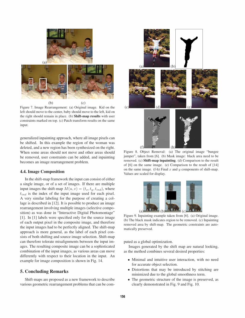
(a)

(b) (c)Figure 7. Image Rearrangement: (a) Original image. Kid on theleft should move to the center, baby should move to the left, kid onthe right should remain in place. (b) Shift-map results with userconstraints marked on top. (c) Patch transform results on the sameinput.

generalized inpainting approach, where all image pixels canbe shifted. In this example the region of the woman wasdeleted, and a new region has been synthesized on the right.When some areas should not move and other areas shouldbe removed, user constraints can be added, and inpaintingbecomes an image rearrangement problem.

4.4. Image Composition

In the shift-map framework the input can consist of eithera single image, or of a set of images. If there are multipleinput images the shift-map M(u, v) = (tx, ty, tind), wheretind is the index of the input image used for each pixel.A very similar labeling for the purpose of creating a col-lage is described in [12]. It is possible to produce an imagerearrangement involving multiple images (selective compo-sition) as was done in “Interactive Digital Photomontage”[1]. In [1] labels were specified only for the source imageof each output pixel in the composite image, and thereforethe input images had to be perfectly aligned. The shift-mapapproach is more general, as the label of each pixel con-sists of both shifting and source image selection. Shift-mapcan therefore tolerate misalignments between the input im-ages. The resulting composite image can be a sophisticatedcombination of the input images, as various areas can movedifferently with respect to their location in the input. Anexample for image composition is shown in Fig. 14.

5. Concluding Remarks

Shift-maps are proposed as a new framework to describevarious geometric rearrangement problems that can be com-

(a) (b)

(c) (d) (e)

(f) (h)Figure 8. Object Removal: (a) The original image “bungeejumper”, taken from [6]. (b) Mask image: black area need to beremoved. (c) Shift-map inpainting. (d) Comparison to the resultof [6] on the same image. (e) Comparison to the result of [14]on the same image. (f-h) Final x and y components of shift-map.Values are scaled for display.

(a) (b) (c)Figure 9. Inpainting example taken from [6]. (a) Original image.(b) The black mask indicates region to be removed. (c) Inpaintingremoved area by shift-map. The geometric constraints are auto-matically preserved.

puted as a global optimization.Images generated by the shift map are natural looking,

as the method combines several desired properties:

• Minimal and intuitive user interaction, with no needfor accurate object selection.

• Distortions that may be introduced by stitching areminimized due to the global smoothness term.

• The geometric structure of the image is preserved, asclearly demonstrated in Fig. 9 and Fig. 10.

156

(a) (b)

(c)Figure 10. Inpainting example taken from [15], where it wasclaimed that user interaction is needed to propagate the structure.Shift-map needs no user interaction. (a) Original image. (b) Theblack mask indicates region to be removed. (c) Completion ofremoved area by shift-map. The geometric constraints are auto-matically preserved.

(a) (b)

(c) (d)Figure 11. Inpainting using shift-map. (a) Original image from[18]. (b) Black pixels need to be removed. (c) Simple inpainting.(d) Generalized inpainting, where other image pixels are allowedto move. A new region was synthesized on the right.

• Large regions can be synthesized. This appears in allexamples, and an isolated demonstration appears inFig. 12.

Hierarchical optimization resulted in a very fast com-putation, especially in comparison to related editing ap-proaches. The applicability of shift map to retargeting, in-painting, and image rearrangement was demonstrated andcompared to state of the art algorithms.

Although shift-map editing performs well on a large va-riety of input, it may miss user’s intensions. Effects can

Figure 12. Image expansion using shift-map as texture synthesis.Input images included several rotations of original image. Left:Original; Right: Synthesized.

(a) (b)

(c)

(d) (e) (f)Figure 14. Image Composition. User constrains are given by speci-fying output locations of selected regions, and other output regionsare generated automatically. (a-b) Original images. (c) An imagecomposed from both (a) and (b). (d-e-f) The regions used as userconstraints for creating (c) from (a) and (b).

be controlled by using saliency maps, or by performing thealgorithm in several steps.

Extending shift-map to use multiple source images, asdescribed in shift map composition, can also be used forinpainting. Input images can include transformations of theoriginal input image like rotation, scaling etc.

References

[1] A. Agarwala, M. Dontcheva, M. Agrawala, S. Drucker,A. Colburn, B. Curless, D. Salesin, and M. Cohen. Interac-tive digital photomontage. In SIGGRAPH, pages 294–302,2004.

[2] S. Avidan and A. Shamir. Seam carving for content-awareimage resizing. ACM Trans. Graph., 26(3):10, 2007.

157

(a) (b) (c) (d) (e)Figure 13. Comparison to other methods: reducing width by 50%. Soft copy can be magnified for better viewing. (a) Original image. (b)Improved Seam Carving [13]. (c) Video-retargeting [19]. (d) Optimized scale-and-stretch [16]. (e) Shift-map.

[3] Y. Boykov and V. Kolmogorov. An experimental comparisonof min-cut/max-flow algorithms for energy minimization invision. IEEET-PAMI, 26(9):1124–1137, Sept 2004.

[4] Y. Boykov, O. Veksler, and R. Zabih. Fast approxi-mate energy minimization via graph cuts. IEEET-PAMI,23(11):1222—1239, 2001.

[5] T. Cho, M. Butman, S. Avidan, and W. Freeman. The patchtransform and its applications to image editing. In CVPR’08,2008.

[6] A. Criminisi, P. Perez, and K. Toyama. Object removal byexemplar-based inpainting. In CVPR’03, volume 2, pages721–728, 2003.

[7] J. Hays and A. Efros. Scene completion using millions ofphotographs. CACM, 51(10):87–94, 2008.

[8] V. Kolmogorov and R. Zabih. What energy functions can beminimized via graph cuts? In ECCV’02, pages 65–81, 2002.

[9] N. Komodakis. Image completion using global optimization.In CVPR’06, pages 442–452, 2006.

[10] V. Kwatra, A. Schodl, I. Essa, G. Turk, and A. Bobick.Graphcut textures: image and video synthesis using graphcuts. In SIGGRAPH’03, pages 277–286, 2003.

[11] H. Lombaert, Y. Sun, L. Grady, and C. Xu. A multilevelbanded graph cuts method for fast image segmentation. InICCV’05, volume 1, pages 259–265, 2005.

[12] C. Rother, L. Bordeaux, Y. Hamadi, and A. Blake. Autocol-lage. In SIGGRAPH’06, pages 847–852, 2006.

[13] M. Rubinstein, A. Shamir, and S. Avidan. Improved seamcarving for video retargeting. In SIGGRAPH’08, pages 1–9,2008.

[14] D. Simakov, Y. Caspi, E. Shechtman, and M. Irani. Summa-rizing visual data using bidirectional similarity. In CVPR’08,2008.

[15] J. Sun, L. Yuan, J. Jia, and H. Shum. Image completion withstructure propagation. In SIGGRAPH’05, pages 861–868,2005.

[16] Y. Wang, C. Tai, O. Sorkine, and T. Lee. Optimized scale-and-stretch for image resizing. ACM Trans. Graph., 27(5):1–8, 2008.

[17] Y. Wexler, E. Shechtman, and M. Irani. Space-time videocompletion. CVPR’04, 1:120–127, 2004.

[18] M. Wilczkowiak, G. Brostow, B. Tordoff, and R. Cipolla.Hole filling through photomontage. In BMVC, pages 492–501, 2005.

[19] L. Wolf, M. Guttmann, and D. Cohen-Or. Non-homogeneouscontent-driven video-retargeting. In ICCV’07, 2007.

158