short-term rentals and the housing market: quasi ... · year of observations 2,016 1.158 2,014...

Short-term rentals and the housing market:

Quasi-experimental evidence from Airbnb in Los Angeles∗

Hans R.A. Koster† Jos van Ommeren‡ Nicolas Volkhausen§

December 11, 2018

Abstract – Online short-term rental (STR) platforms such as Airbnb have grown spectacularly.

We study the effects of STR-platforms on the housing market using a quasi-experimental research

design. 18 out of 88 cities in Los Angeles County have severely restricted short-term rentals by

adopting Home Sharing Ordinances. We apply a panel regression-discontinuity design around

the cities’ borders. Ordinances reduced listings by 50% and housing prices by 3%. Difference-in-

differences estimates show that ordinances reduced rents by 3%. These estimates imply large

effects of Airbnb on property values in areas attractive to tourists (e.g. an increase of 14% within

5km of Downtown LA).

Keywords – short-term rentals, house prices, regulation, supply effects, externalities.

JEL codes – R21, R31, Z32.

∗This work has benefited from a Veni research grant from the Netherlands Organisation for Scientific Research.We thank Jan Brueckner, David Gomtsyan, Eric Koomen, Robert Elliott, Stephen Sheppard, Mariona Segu, aswell as the seminar audiences at the Higher School of Economics (St. Petersburg), the Southwestern University ofFinance and Economics (Chengdu), the 13th Meeting of the Urban Economic Assocation (New York), Universityof Birmingham, and Zhejiang University (Hangzhou) for useful comments.†Department of Spatial Economics, Vrije Universiteit Amsterdam, De Boelelaan 1105 1081 HV Amsterdam,

The Netherlands email: [email protected]. Hans is also research fellow at the National Research University –Higher School of Economics (Russia) and the Tinbergen Institute, and affiliated to the Centre for Economic PolicyResearch and the Centre for Economic Performance at the London School of Economics.‡Department of Spatial Economics, Vrije Universiteit Amsterdam, De Boelelaan 1105 1081 HV Amsterdam,

email: [email protected]. Jos is also research fellow at the Tinbergen Institute.§Department of Spatial Economics, Vrije Universiteit Amsterdam, De Boelelaan 1105 1081 HV Amsterdam,

The Netherlands email: [email protected].

[email protected]

[email protected]

[email protected]

1 Introduction

Short-term housing rentals (STRs) have become very important due to the rise of online STR-

platforms which provide opportunities for households to informally offer accommodation to

visitors. The largest online platform is Airbnb. The surge in popularity of STR-platforms has led

to substantial opposition because of a decrease in housing affordability (Samaan 2015, Sheppard

& Udell 2016), unfair competition, and illegal hotelization (CBRE 2017). Negative externalities

(e.g. noise, reduction in perceived safety) due to the presence of tourists in residential buildings

are also frequently mentioned (see e.g. Lieber 2015, Williams 2016, Filippas & Horton 2018).

Local governments around the globe have responded quite differently towards regulating STRs.

Most cities have not significantly regulated these platforms, but a limited number of cities have

recently put severe restrictions in place. Berlin, for instance, requires STR-hosts to occupy the

property for at least 50% of the time (O’Sullivan 2016). San Francisco imposes a 14% hotel

tax (i.e. a Transient Occupancy Tax ) and a cap of maximum 90 rental days per year (Fishman

2015). Amsterdam even imposes a maximum cap of 30 rental days per year.

The theoretical effect of a regulation that restricts the use of STR-platforms is implied by a

literature on the effects of land use regulation on the housing market (see e.g. Turner et al. 2014).

In the absence of negative externalities, and given an upward-sloping housing supply curve,

economic theory tells us that such regulation induces a reduction in house prices and rents,

because it restricts an efficient use of housing.1 This reduction will be particularly pronounced

at locations that are attractive to tourists and other visitors. Theory then indicates that there

is a discrete decrease in house prices at HSO borders, because houses within an HSO area offer

less value to homeowners. Spatial equilibrium theory indicates that there is no discrete jump at

HSO borders for (long-term) rents, as houses offer the same value to renters across the border,

at least given the conditions that renters are not allowed to list their property on Airbnb and

that houses across borders are otherwise perfect substitutes.2

1The presence of substantial negative externalities may, however, lead to the opposite effect when a reductionin negative external costs due to regulation would increase residential demand. STR-platforms may also haveeffects on prices in the wider housing market, because a higher demand for housing implies that the price demandcurve in the whole housing market will shift upwards (see e.g. Hilber & Vermeulen 2016). We think that, atleast for Los Angeles, this effect is negligible, because only one in a thousand properties is directly affected byregulation: 4.5% of the properties are in regulated areas, of which maximally 2.5% are listed.

2In line with that we will show that HSOs induce rents decreases, except close to the border of an HSO area.

1

In the current paper, we focus on the effect of regulating STR-platforms on the housing market

using a quasi-experimental research design for 18 out of 88 cities in Los Angeles County that

have imposed restrictions on short-term rentals. Those cities implement so-called Home Sharing

Ordinances (HSOs) that essentially ban informal vacation rentals; hosts renting out entire

properties are now subject to the same formal regulations as regular hotels and bed and

breakfasts. Short-term home sharing is not always prohibited, albeit restricted in those cities.

There are several reasons why we focus on Los Angeles County. First, it is an area that is

attractive to tourists and has thousands of listings on Airbnb. It is in the Global Top 10 of the

cities with the most Airbnb listings and is the second city in the US after New York. Second,

there is substantial spatio-temporal variation in the implementation of HSOs within this county.

For example, HSOs have been implemented in cities that receive many tourists (e.g. Santa

Monica), as well as in cities that are more at the edge of the Los Angeles Conurbation (e.g.

Pasadena). We think this might add to external validity of the results shown in the paper.

Third, by focusing on 18 cities, rather than on the introduction of an HSO in one single city, we

substantially reduce the likelihood that our results are contaminated by an unobserved event

(e.g., a change in a city-specific policy) that occurs around the same time as the introduction of

the HSO.

The variation in restrictions between cities enables us to use a spatial regression discontinuity

design (RDD), which we combine with a difference-in-differences (DiD) set-up: we essentially

focus on changes in the number of Airbnb listings, as well as in house prices, close to the borders

of cities that have implemented HSOs. More specifically, we use micro-data on Airbnb listings

and house prices between 2014 and 2018. Our main results are then based on observations

within approximately 2 km of borders of HSO areas. We distinguish between effects on different

types of listings (home sharing, entire properties) as well as on the prices in different areas (e.g.,

with high and low tourist demand).

We have two main results. Our first result is that HSOs are very effective in reducing Airbnb

listings. The ordinances strongly reduced the number of Airbnb listings of entire properties

by about 70% in the long run. Its effect on home sharing listings is smaller and about 50%.

We further show that home sharing listings have not been reduced when home sharing is still

2

allowed, which is the case in 4 out of the 18 cities with HSOs.3

Our second result is that the HSO reduced house prices by about 3% on average. This effect

is more pronounced in neighborhoods that are attractive to tourists. The effect of an HSO

increases by 30% when tourist demand – proxied by the density of tourist pictures – increases

by 1 standard deviation. Hence, tourist demand for accommodation increases residential prices,

because of competing demands for space.

To explore this issue further, we estimate a ‘structural equation’ capturing the effect of demand

for short-term rentals on housing prices. We measure short-term rental demand using the

Airbnb listings rate with respect to the number of buildings within 200m. Using the HSO as a

supply-shifting instrument for the listings rate around the border, we show that short-term rental

demand for accommodation increases prices of residential properties – a standard deviation

increase in Airbnb listings increases prices by about 5.5%.

Using ancillary data on aggregate rents for zip codes and a DiD estimation strategy we show that

rents decrease by the same amount as house prices. The DiD approach relies on more restrictive

identifying assumptions than the Panel RDD approach. One way to check the reliability of

the DiD approach in this context is by applying the same approach to house prices. We find

that it delivers essentially the same results as those obtained using the Panel RDD approach.

This makes it plausible that the i) DiD approach generates causal effects and that ii) the local

average treatment effect obtained in the Panel RDD approach can be interpreted as the average

treatment effect that also holds away from HSO borders.4

We then show that Airbnb imply modest property value increases for LA County as a whole: the

average property value increase due to Airbnb is 3%. However, this masks the fact that a large

part of LA County is not very urbanized and does not attract tourists. By contrast, the effects of

Airbnb on the housing market can be large in central urban areas – within 5km of Los Angeles’s

Central Business District (CBD), property values have increased by 14% due to Airbnb. Within

5km of beaches, prices have increased by about 6.5%. The decision to implement an HSO is a

3We also show that Airbnb accommodation prices are not affected by the HSOs, which suggests that the marketfor short-term rentals is highly competitive and that tourist demand for local accommodation is highly elastic.On the other hand, we find suggestive evidence that the number of formally registered traveler accommodationsincrease due to HSOs.

4Furthermore, we demonstrate that there are no effects on rents around the HSO border, confirming thatrental properties close to HSO borders are close substitutes.

3

political one, with a clear group of winners and losers, and strong distributional effects: owners

lose from HSO-induced house price reductions, whereas renters benefit from lower rents.

Related literature. In recent years, the sharing economy has received increasing attention.

Economists have examined home sharing from various angles such as racial discrimination in the

online marketplace (Edelman et al. 2014, Kakar et al. 2016), negative externalities of tourism

(Van der Borg et al. 2017, Gutierrez et al. 2017) and its effects on the hotel industry (Zervas

et al. 2017). There has been little empirical research on the effect of short-term rentals and

related policies on the housing market, while studies that surmount the various endogeneity

issues are, to the best of our knowledge, not yet existing.5 Our study is the first one that exploits

quasi-experimental variation provided by changes in regulation to estimate the effect of HSOs

on the housing market.

Our paper also relates to a literature studying the effects of tourism and amenities on housing

markets. Carlino & Saiz (2008), for example, show that the number of tourists visiting a

city is a good predictor of the growth of US metropolitan areas in the 1990s. Ahlfeldt et al.

(2016) and Gaigne et al. (2018) find that the density of pictures taken by tourists and residents

increases land value and attracts the wealthy. Moreover, a large number of papers show that high

amenity locations have higher housing values (see e.g. Van Duijn & Rouwendal 2013, Ahlfeldt &

Kavetsos 2014, Koster & Rouwendal 2017). In these studies, it is impossible to disentangle the

effects of tourism and amenities. Our paper therefore contributes to this literature by using a

quasi-experimental research set-up, enabling us to isolate the effects of tourism demand, proxied

by Airbnb listings.6

Conceptually, our paper is close to a literature measuring the effect of land use regulation and

5Sheppard & Udell (2016) use a DiD approach and conclude that housing values increased by about 31% due toAirbnb. One issue, which seems not convincingly addressed, is that neighborhoods tend to become more attractiveto residents and tourists at the same time. Horn & Merante (2017) show that a high Airbnb density increasesasking rents by 1.3-3.1%. Garcia-Lopez et al. (2018) uses temporal variation in rents together with an instrumentalvariables approach to show that Airbnb causes a 4% increase in rents in Barcelona. Barron et al. (2018) show thatAirbnb increases house prices and rents in US cities. A few reports – lacking a convincing identification strategy –have studied the impact of Airbnb. New York Communities for Change looked at correlations between Airbnb andneighborhood mean rent increases (NYCC 2015). Samaan (2015) looks at the rental market in Los Angeles andreports a 4 percentage points faster growth of rents in popular Airbnb neighborhoods. Lee (2016) argues thatAirbnb reduces the affordable housing supply in Los Angeles, because landlords remove units from the housingmarket by listing on Airbnb. Wachsmuth & Weisler (2017) argue that Airbnb has introduced new revenue flows tothe housing market which are systematic but geographically uneven.

6As far as we know, the current literature is silent on the causal effect of tourist accommodation demand onthe housing market.

4

zoning, as the HSO can be seen as an example of a zoning regulation. Most studies in this field

show that housing supply constraints are associated with increasing housing costs, a strong

reduction in new construction, and rapid house price growth (Glaeser et al. 2005, Green et al.

2005, Ihlanfeldt 2007, Hilber & Vermeulen 2016). However, they do not identify the underlying

mechanisms that lead to price increases. Glaeser & Ward (2009) find that local constraints

do not increase the price between localities, because areas that are geographically close are

reasonably close substitutes. Using a spatial regression discontinuity design, Koster et al. (2012)

and Turner et al. (2014) also study the local effects of regulation and find that the effects of

regulation for homeowners may be up to 10% of the housing value. One major difference with

these studies is that our research design does not rely on cross-sectional variation in land use

regulation, but rather identifies the effect based on changes in regulation over time.

This paper proceeds as follows. In Section 2 we discuss the research context. Section 3 introduces

the data and provide descriptives. In Section 4 we elaborate on the identification strategy,

followed by graphical evidence in Section 5. We report and discuss the main results in Section 6,

which is followed by back-of-the-envelope welfare calculations and distributional implications of

the HSO and Airbnb in Section 7. Section 8 concludes.

2 Context

2.1 Airbnb in Los Angeles County

In 2007, Brian Chesky and Joe Gebbia came up with the idea of putting an air mattress in

their living room and turning it into a bed and breakfast, marketed through an online platform

(Lagorio-Chafkin 2010). The website – later called Airbnb and officially launched in 2008 – is a

platform that connects hosts that own accommodation (rooms, apartments, houses) with guests

seeking temporal accommodation. Prospective hosts list their spare rooms or entire apartments

for a self-established price and offer the lodging to potential guests.7 Airbnb charges a fee to

both the host and guest.

Airbnb has grown rapidly since its launch in Los Angeles County (as in other major cities across

7With more than 4 million listings – more properties than the top 3 hotel brands, Marriott, Hilton, andIHG, combined (Airbnb 2017) – Airbnb emerged as one of the main figureheads of the sharing economy, in whichtechnology companies disrupt well-established business models by facilitating direct, peer-to-peer exchanges ofgoods and services (Lee 2016).

5

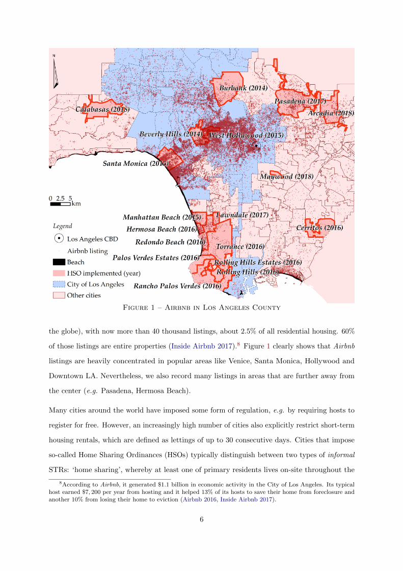
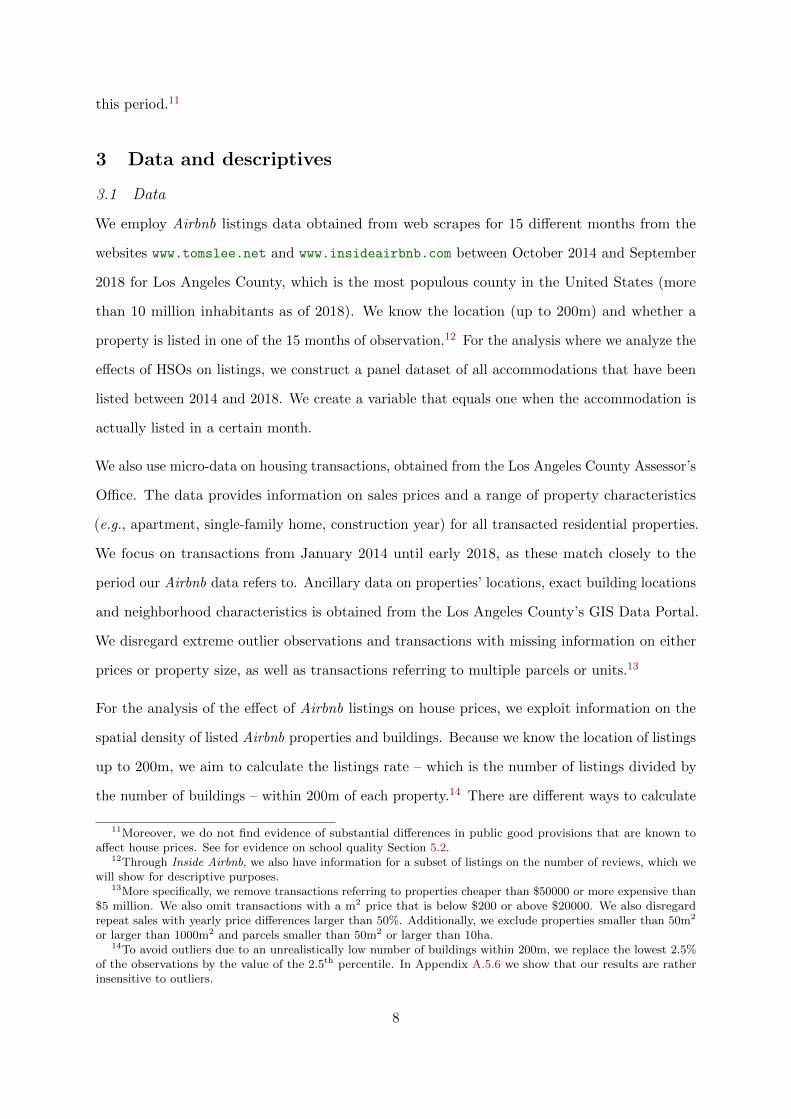
Figure 1 – Airbnb in Los Angeles County

the globe), with now more than 40 thousand listings, about 2.5% of all residential housing. 60%

of those listings are entire properties (Inside Airbnb 2017).8 Figure 1 clearly shows that Airbnb

listings are heavily concentrated in popular areas like Venice, Santa Monica, Hollywood and

Downtown LA. Nevertheless, we also record many listings in areas that are further away from

the center (e.g. Pasadena, Hermosa Beach).

Many cities around the world have imposed some form of regulation, e.g. by requiring hosts to

register for free. However, an increasingly high number of cities also explicitly restrict short-term

housing rentals, which are defined as lettings of up to 30 consecutive days. Cities that impose

so-called Home Sharing Ordinances (HSOs) typically distinguish between two types of informal

STRs: ‘home sharing’, whereby at least one of primary residents lives on-site throughout the

8According to Airbnb, it generated $1.1 billion in economic activity in the City of Los Angeles. Its typicalhost earned $7, 200 per year from hosting and it helped 13% of its hosts to save their home from foreclosure andanother 10% from losing their home to eviction (Airbnb 2016, Inside Airbnb 2017).

6

visitor’s stay, and ‘vacation rentals’, which are for exclusive use of the visitor.

In Figure 1 we show the names of 18 cities that have imposed HSOs during our study period

2014-2018. The other 60 cities – including the largest one, the City of Los Angeles – did not

impose regulations in this period.9 These 18 cities, which contain close to 5 percent of the whole

housing stock of this County, essentially ban informal vacation rentals by requiring hosts to

have a business license and comply with health and safety laws, as well as levying a Transient

Occupancy Tax on the listing price (up to 15%). Most cities completely ban both home sharing

and vacation rentals. 4 out of 18 cities (Calabasas, Pasadena, Santa Monica and Torrance)

still allow for home sharing, although restrictions apply. In Santa Monica, for example, the

HSO allows for home sharing up to 30 days per year but prohibits hosts to operate more than

one home-share at the same time. The HSOs in LA county are usually enforced. For example,

the City of Santa Monica has collected more than $4.5 million in taxes from Airbnb and other

short-term home rental businesses and has fined hosts violating the law for $80, 000. Vacation

rentals or home-shares that are operating illegally, including informal vacation rentals, may be

issued fines of up to $500 per day and face criminal prosecution if they do not cease operations

(City of Santa Monica 2017).10 In Appendix A.2 we report for each city in LA county more

details regarding STR regulation. We also list our data sources there.

Our empirical approach relies on the fundamental assumption that around the implementation of

the HSOs other policies did not change in the 18 cities compared to their immediate surroundings.

We are not aware of such policy changes (but have actively searched for this). We also offer

statistical support for this assumption. In Section 6.4 we perform a range of placebo tests using

information on price changes around the borders of other sets of cities and using the same

borders but for other time periods. All these tests indicate that, with the exception of the

treated cities, there are no changes in listings and prices at the borders investigated. This makes

it implausible that other policies (or e.g. differences in school quality) changed exactly around

9In 45 cities, short-term renting is technically illegal, because it is not mentioned in the residential housingcode. However, in phone interviews undertaken by the authors, local officials state that nothing is done to enforcethe residential housing code and to prevent homeowners to list their properties on Airbnb. This appears to becommon knowledge. We make sure that listings in those 45 cities are not lower compared to other places (seeSection 6.4).

10Note that our estimates of the HSOs reflect the actual levels of enforcement of the cities investigated in LosAngeles County. For example, it is plausible that the effects on number of listings as well as property prices arehigher in cities where enforcement is more strict.

7

this period.11

3 Data and descriptives

3.1 Data

We employ Airbnb listings data obtained from web scrapes for 15 different months from the

websites www.tomslee.net and www.insideairbnb.com between October 2014 and September

2018 for Los Angeles County, which is the most populous county in the United States (more

than 10 million inhabitants as of 2018). We know the location (up to 200m) and whether a

property is listed in one of the 15 months of observation.12 For the analysis where we analyze the

effects of HSOs on listings, we construct a panel dataset of all accommodations that have been

listed between 2014 and 2018. We create a variable that equals one when the accommodation is

actually listed in a certain month.

We also use micro-data on housing transactions, obtained from the Los Angeles County Assessor’s

Office. The data provides information on sales prices and a range of property characteristics

(e.g., apartment, single-family home, construction year) for all transacted residential properties.

We focus on transactions from January 2014 until early 2018, as these match closely to the

period our Airbnb data refers to. Ancillary data on properties’ locations, exact building locations

and neighborhood characteristics is obtained from the Los Angeles County’s GIS Data Portal.

We disregard extreme outlier observations and transactions with missing information on either

prices or property size, as well as transactions referring to multiple parcels or units.13

For the analysis of the effect of Airbnb listings on house prices, we exploit information on the

spatial density of listed Airbnb properties and buildings. Because we know the location of listings

up to 200m, we aim to calculate the listings rate – which is the number of listings divided by

the number of buildings – within 200m of each property.14 There are different ways to calculate

11Moreover, we do not find evidence of substantial differences in public good provisions that are known toaffect house prices. See for evidence on school quality Section 5.2.

12Through Inside Airbnb, we also have information for a subset of listings on the number of reviews, which wewill show for descriptive purposes.

13More specifically, we remove transactions referring to properties cheaper than $50000 or more expensive than$5 million. We also omit transactions with a m2 price that is below $200 or above $20000. We also disregardrepeat sales with yearly price differences larger than 50%. Additionally, we exclude properties smaller than 50m2

or larger than 1000m2 and parcels smaller than 50m2 or larger than 10ha.14To avoid outliers due to an unrealistically low number of buildings within 200m, we replace the lowest 2.5%

of the observations by the value of the 2.5th percentile. In Appendix A.5.6 we show that our results are ratherinsensitive to outliers.

8

www.tomslee.net

www.insideairbnb.com

Airbnb intensity. We think that the listings rate captures the fact that a larger share of the

building stock is used as Airbnb. Probably it would be preferable to use housing units rather than

buildings. However, granular data on housing units is unfortunately not available. Moreover,

Airbnb listings may occasionally be inside commercial buildings as well.15

There are however two technical issues. First, the data on listings is based on 14 snapshots during

our study period. Second, we do not have information on listings from January to October 2014.

We first construct an imputed measure which imputes the listing probability based on the nearest

two dates for which we have information.16 We also will use an approximated measure that is

available for the whole period for which we observe house prices, following Zervas et al. (2017)

and Barron et al. (2018). . This approximated measure of number of Airbnb listings in vicinity

(within 200m of each transacted property) is derived from information on listings on the date of

their first review (if this information is missing, we use the date at which the host became active

on Airbnb) and last review, while assuming that the property is continuously listed between the

first and last review. We note that the results using different measures are essentially the same.

We further gather monthly data on listed median rents and house prices at the zip code level

from Zillow, which is a large real estate database company. Zillow has micro-data on over 110

million homes across the United States, not just those homes currently for sale but also for

rent.17 For each zip code in each month, Zillow posts the median listed rent and median listed

sales price.

Finally, for an ancillary analysis we gather data from Eric Fisher’s Geotagger’s World Atlas,

which contain all geocoded pictures on the website Flickr between 2000 and 2016, with most

pictures being taken between 2007 and 2013. To isolate the pictures taken by tourists, we exclude

the users that upload pictures in 6 consecutive months during our study period. We count the

number of pictures within 200m as a proxy for tourist demand. The idea is that locations with

a high picture density likely have more tourists visiting the area.

15One may argue that the listings rate does not account for the fact that buildings are taller in dense areas.Hence, one may be concerned that our results may pick up some effect of urban density. Given that we includevery detailed spatial fixed effects and identify the effects over time, we do not consider this as an issue.

16For example, when we observe in our data that a property is listed in March, but not listed in May, theimputed listing probability is 0.5 in April 2015.

17The most detailed data publicly available is at the so-called Zillow -neighborhood. Because these data areonly available for a few neighborhoods in LA County, we use data at the zip code level.

9

Table 1 – Descriptive statistics for Airbnb data

Panel A: Inside HSO areas mean sd min max

Price per night (in $) 171.8 140.1 0 999HSO implemented 0.769 0.421 0 1Property type – apartment 0.515 0.500 0 1Property type – single-family home 0.408 0.491 0 1Property type – unknown 0.0769 0.266 0 1Rental type – entire home/apartment 0.617 0.486 0 1Rental type – home sharing 0.383 0.486 0 1Accommodation size (in number of persons) 3.421 2.346 1 16Number of reviews 19.27 37.62 1 602Distance to border of HSO area (in km) 0.712 0.643 0.0000622 3.140Distance to the beach (in km) 12.19 12.56 0 44.78

Panel B: Outside HSO areas mean sd min max

Price per night (in $) 145.8 132.7 0 999HSO implemented 0 0 0 0Property type – apartment 0.476 0.499 0 1Property type – single-family home 0.435 0.496 0 1Property type – unknown 0.0886 0.284 0 1Rental type – entire home/apartment 0.597 0.491 0 1Rental type – home sharing 0.403 0.491 0 1Accommodation size (in number of persons) 3.477 2.505 1 20Number of reviews 21.62 40.45 1 700Distance to border of HSO area (in km) 4.616 4.947 0.000143 64.83Distance to the beach (in km) 15.31 10.68 0 96.40

Notes: The number of listings for HSO areas is 53, 980. Outside HSO areas it is 344, 813.

3.2 Descriptives

Table 1 reports the main descriptive statistics for the Airbnb listings. We observe that, on

average, rental prices per night in areas where HSOs are implemented are somewhat higher

than other areas. Hence, the HSOs are predominantly implemented in areas where homeowners

really care most about the HSO. In other observable characteristics, such as accommodation

size, number of reviews and the share of entire properties, listings seem to be similar in both

areas. The most notable difference is that the distance to the beach is lower in areas where

HSOs are implemented, as several beach towns, such as Santa Monica, Manhattan Beach and

Redondo Beach, have implemented HSOs. This difference may be relevant as distance to the

beach is one characteristic that possibly affects tourist demand for accommodation. We note

that the apartment share of Airbnb listings is about 0.5, which exceeds the apartment share of

housing transactions (see Table 2). Hence, the forbidding of Airbnb in apartment buildings by

Owners Associations (e.g. to reduce within-building externalities) is unlikely to be an important

phenomenon.

10

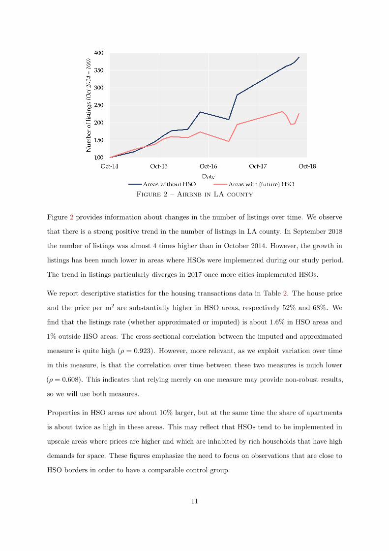
Figure 2 – Airbnb in LA county

Figure 2 provides information about changes in the number of listings over time. We observe

that there is a strong positive trend in the number of listings in LA county. In September 2018

the number of listings was almost 4 times higher than in October 2014. However, the growth in

listings has been much lower in areas where HSOs were implemented during our study period.

The trend in listings particularly diverges in 2017 once more cities implemented HSOs.

We report descriptive statistics for the housing transactions data in Table 2. The house price

and the price per m2 are substantially higher in HSO areas, respectively 52% and 68%. We

find that the listings rate (whether approximated or imputed) is about 1.6% in HSO areas and

1% outside HSO areas. The cross-sectional correlation between the imputed and approximated

measure is quite high (ρ = 0.923). However, more relevant, as we exploit variation over time

in this measure, is that the correlation over time between these two measures is much lower

(ρ = 0.608). This indicates that relying merely on one measure may provide non-robust results,

so we will use both measures.

Properties in HSO areas are about 10% larger, but at the same time the share of apartments

is about twice as high in these areas. This may reflect that HSOs tend to be implemented in

upscale areas where prices are higher and which are inhabited by rich households that have high

demands for space. These figures emphasize the need to focus on observations that are close to

HSO borders in order to have a comparable control group.

11

Table 2 – Descriptive statistics for housing transactions


House price (in $) 1,023,911 673,903 50,000 5,000,000House price per m2 (in $) 6,187 2,725 274.3 20,000HSO implemented 0.391 0.488 0 1Listings rate <200 (imputed) 1.652 4.016 0 47.89Listings rate <200 (approximated) 1.509 3.866 0 48Property size (in m2) 167.6 78.79 50 842Parcel size (in m2) 1,447 3,247 57 54,655Apartment 0.371 0.483 0 1Number of bedrooms 2.934 1.014 1 9Number of bathrooms 2.447 0.968 1 5Construction year of property 1,971 22.07 1,897 2,017Distance to border of HSO area (in km) 0.718 0.619 0.000137 2.992Distance to the beach (in km) 14.61 14.14 0.0140 45.50Year of observations 2,016 1.158 2,014 2,018


House price (in $) 610,285 476,541 50,000 5,000,000House price per m2 (in $) 4,064 2,189 247.5 20,000HSO implemented 0 0 0 0Listings rate <200 (imputed) 1.087 5.098 0 261.2Listings rate <200 (approximated) 0.977 4.541 0 193.3Property size (in m2) 152.7 69.39 50 921Parcel size (in m2) 2,110 6,333 50 95,285Apartment 0.208 0.406 0 1Number of bedrooms 2.980 0.948 1 10Number of bathrooms 2.198 0.901 1 5Construction year of property 1,968 23.63 1,884 2,018Distance to border of HSO area (in km) 11.09 12.33 0.000952 70.67Distance to the beach (in km) 27.46 19.99 0.00346 107.5Year of observations 2,016 1.169 2,014 2,018

Notes: The number of transactions for HSO areas is 32973. Outside HSO areas it is 250, 509.

Finally, we turn to the data on rents and list prices from Zillow. We report descriptives in

Table 3. The average rent per m2 is $26 in HSO areas, compared to $25 outside HSO areas.

The listings rate is lower in HSO areas (0.8%), then outside these areas (1.4%). The zip code

with the maximum rate, 48%, is in Hollywood (City of LA), followed by a zip code in Venice

(City of LA) with 28%. Although rents are very similar for both areas, we find a 17% lower

average house price per m2 outside HSO areas. A priori, it is difficult to judge the quality of the

information offered by Zillow. Quite assuringly, the correlation between median listed prices in

Zillow and median transaction prices using the Assessor Office’s data (which we use for micro

analyses) is high (ρ = 0.941). However, when we demean prices by zip code and month fixed

effects, the correlation is only moderate (ρ = 0.322). This suggests that results might be dataset

specific. However, we will show that our results are not driven by the choice of the dataset.

12

Table 3 – Descriptive statistics for Zillow data


Rent per m2 (in $) 26.32 8.837 15.79 65.31List price per m2 (in $) 6,692 2,464 4,035 17,830HSO implemented 0.579 0.494 0 1Listings rate 1.281 1.605 0 6.993Distance to border of HSO area (in km) 1.029 0.399 0.374 2.029Distance to the beach (in km) 25.54 7.136 12.85 41.08Buildings per (in ha) 14.31 10.44 1.239 40.98


Rent per m2 (in $) 24.67 9.543 7.927 76.52List price per m2 (in $) 5,563 2,622 1,089 15,428HSO implemented 0 0 0 0Listings rate 2.815 5.054 0 47.91Distance to border of HSO area (in km) 10.28 13.56 0.0594 58.65Distance to the beach (in km) 29.41 17.17 1.420 80.59Buildings per (in ha) 11.48 9.730 0.320 45.66

Notes: The number of transactions for HSO areas is 815. Outside HSO areas it is 2676.

4 Econometric framework

The main econometric issue when aiming to estimate a causal effect of Airbnb on the housing

market is that Airbnb listings are not randomly allocated across space but are concentrated in

neighborhoods that are attractive to both residents and visitors with a demand for short-term

letting. One way to address this issue is to compare adjacent cities that differ in regulation

of Airbnb and then use a Spatial RDD around the cities’ borders. This ignores however that

cities differ in other ways than in their regulation of Airbnb. We address the latter by exploiting

variation over time in the HSO around the borders of HSO areas. The HSOs induced exogenous

changes in the propensity to list a property on Airbnb, which may have resulted in changes in

house prices. Consequently, as we will use panel data (for listings as well as house prices), we

will employ a Spatial Panel Regression-Discontinuity Design.

4.1 HSOs and Airbnb listings

The first step is to estimate the effect of the HSO on a property’s probability of being listed

on Airbnb. We distinguish between the probability of being listed as an entire home and the

probability of being listed as home sharing. We will estimate linear probability models, where

we estimate the effects of the HSO on both probabilities separately.18 We use a Spatial RDD,

18Our main motivation not to estimate multinomial discrete choice models but to estimate separate models isthat it appears that properties never switch from being listed as an entire home to home sharing, or the other

13

where the running variable is the distance to the nearest border of an area where an HSO is

implemented or will be implemented in the future. The effect of the HSO is captured by a

discrete jump in the probability of being listed after its introduction. Let ìkt be a dummy

variable indicating whether a property i near a border of an HSO area k is listed in month t and

hikt be a dummy indicating whether the HSO has been implemented.

One may argue that differences in unobservables of properties between HSO areas and neigh-

boring cities may be correlated to the implementation of an HSO. For example, differences in

attractiveness of certain locations that are discrete at, or even further away from, the border

(e.g., school quality) may be present, which are correlated to hikt and influence ìkt at the same

time. We therefore include property fixed effects λi, which control for difficult-to-observe but

time-invariant differences between locations, and µkt, which capture HSO-border area specific

months fixed effects (i.e. a fixed effect for each web scrape in each HSO-border area). This

implies:

(α, λik, µkt) = arg minα,λi,µkt

N∑n=1

K

(dikb

)× (ìkt − αhikt − λi − µkt)2, (1)

where α is the parameter of interest and K( · ) is a uniform kernel function:

K

(dikb

)= 1dik<b, (2)

where dik is the distance to the border and b a given bandwidth. Note further that because we

include property fixed effects, we effectively only use data on properties that have been listed at

least once.

The bandwidth b determines how many observations are included on both sides of the border. In

an RDD, estimated parameters are often sensitive to the choice of the bandwidth. We therefore

show results for different bandwidths. Our preferred specification is based on an approach

proposed by Imbens & Kalyanaraman (2012) to determine the optimal bandwidth, b∗, which is

calculated conditional on control variables (property fixed effects and HSO-area×month fixed

effects). We discuss the procedure to determine b∗ in more detail in Appendix A.3.

way around. This also implies that the HSO did not induce hosts of entire properties to shift to home sharing,which is a theoretical possibility. The results are very similar if we estimate Logit models, or estimate ConditionalLogit Models of location choice using Poisson regressions. Results are available upon request.

14

4.2 HSOs, Airbnb and house prices

We employ a similar approach to measure the effect of the HSO on house prices. Let pijt be

the house price of property i in census block j near a border of an HSO area k in month t with

time-invariant housing characteristics xijk. We estimate:

(β, ζ, ηj , θkt) = arg minβ,ζ,ηj ,θt

N∑n=1

K

(dikb

)× (log pijkt − βhijkt − ζxijk − ηj − θkt)2, (3)

where β is the parameter of interest, and ηj and θkt refer to census block and HSO border×

month fixed effects respectively. This equation implies that we compare price changes along the

borders of HSO areas to see if prices have changed in the treated areas due to the HSO.19 Again,

we will show results given different bandwidths, but our preferred specification is based on the

optimal bandwidth.

The results from equation (3) are informative on the local average treatment effect of the HSO

on house prices, where the average applies to estimates along the borders of HSO areas. However,

it is plausible that the effect strongly varies over space depending on local tourist demand for

accommodation, which strongly covaries with the demand for Airbnb, denoted by the listings

rate rijkt. Neighborhoods with a low Airbnb listings rate (because of low tourist demand) should

hardly be affected by the HSO, while areas that are popular with tourists should be much more

affected, potentially reducing the external validity of the local average treatment effect.

We will therefore also estimate a ‘structural equation’ where we regress prices on imputed listings

in the direct vicinity. Because rijkt is endogenous (as listings are imputed and because residents

and visitors may have a preference for similar locations), we instrument rijkt with hijkt. The

second stage is then given by:

(γ, ζ, ηj , θkt) = arg minγ,ζ,ηj ,θt

N∑n=1

K

(dikb

)× (log pijkt − γrijkt − ζxijk − ηj − θkt)2, (4)

where rijkt is obtained from:

(ˆδ,

ˆζ, ˆηj ,

ˆθkt) = arg min

δ,ζ,ηj ,θt

N∑n=1

K

(dikb

)× (rijkt − δhijkt − ζxijk − ηj − θkt)2, (5)

19Anticipation effects of new laws may underestimate the effects of HSOs. We test for this in Section 6.2.

15

where the ∼ refer to first-stage coefficients.

4.3 HSOs, Airbnb and rents

Given the assumption of a spatial equilibrium, long-term rents should not be different at HSO

borders, because rental properties at different sides but very close to these borders offer the

same value to renters. Given that we have information on rents at the zip code level (which

would make the use of a discontinuity design anyway less convincing), we pursue an alternative,

but more standard, design where we regress rents, rjt, on hjt. We then have:

(φ, ηj , θkt) = arg minφ,ηj ,θt

N∑n=1

(log rjt − φhjt − ηj − θkt)2, (6)

where φ is the parameter of interest, ηj are zip code fixed effects and θkt are month fixed effects.

This is standard difference-in-differences specification, with the notion that we have multiple

treatments at different times in our study period.20 In line with the previous set-up we will also

estimate a ‘structural equation’ by regressing rents on the listings rate.

The key assumption underlying a DiD strategy is that there is a common trend between the

treatment and control group. We test for this in Section 5.3, but still we think that the above

strategy is less convincing than the Panel RDD. We therefore will make sure that with this

alternative strategy the price effects are comparable to the ones obtained using the more credible

Panel RDD approach.

5 Graphical evidence

5.1 Treatment effects

Before we turn to the regressions results, we illustrate our research design graphically. In Figure

3, we first focus on the impact of the HSO on Airbnb listings. We include census block group

and HSO border×month fixed effects, and include a 4th-order polynomial of distance to the

border outside HSO areas and a 2rd-order polynomial of distance to the border inside HSO areas

(as we have fewer data points that are closer to the border inside HSO areas).21 In Figure 3a,

20We make sure that using a weighted measure based on number of housing units leads to similar results.21The choice of the order of the polynomial does not make any difference. This indicates that displacement

effects – Airbnb hosts that move their listings to just outside an HSO area – are unlikely to be important, asdisplacement effects would have induced an increase in listings just outside treated areas.

16

(a) Entire home/apartment listings (b) Home sharing listings

(c) Price per night (in $) (d) Accommodation size

Figure 3 – Airbnb listings: variation near the HSO bordersNotes: Negative distances indicate areas outside HSO areas and areas inside HSO areas before treatment. The dots areconditional averages at every 200m interval. We include census block group and HSO border×month fixed effects. Thedotted lines denote 95% confidence intervals.

we plot the probability of listing ‘entire properties’ on Airbnb. We observe a sizable drop in type

of listings in areas where HSOs have been implemented. The difference is about 10 percentage

points.22 Given a listing probability of about 0.30 (for residences that have been listed at least

once), this implies a reduction in ‘entire properties’ listings of 33%. Hence, in line with anecdotal

evidence, this suggests that the HSO was very effective in reducing STRs. In Figure 3b we plot

the probability of listing ‘home sharing’ on Airbnb. Then, we find a smaller drop in listings of

about 7.5 percentage points, corresponding to a reduction in ‘home sharing’ listings of about

25%.

In Figures 3c and 3d, we investigate whether there are differences in the change of characteristics

of houses listed on Airbnb between HSO areas and areas in the close vicinity. This does not seem

to be the case – there is essentially no difference in how Airbnb prices per night and availability

22In Appendix A.4 we also compare the probability of being listed before and after the HSOs were implementedon both sides of the border, without conditioning on census block group fixed effects. This analysis suggeststhere was essentially no difference between HSO areas and surrounding areas in terms of number of listed entireproperties before the implementation, whereas the probability is about 10-20 percentage points lower after it wasimplemented, in line with Figures 3a and 3b.

17

Figure 4 – House prices: variation near the HSO bordersNotes: Negative distances indicate areas outside HSO areas and areas inside HSO areas before treatment. The dots areconditional averages at every 200m interval. We include census block group and HSO border×month fixed effects. Thedotted lines denote 95% confidence intervals.

changed over time between HSO areas and neighboring areas.

We repeat the exercise, but now focus on house prices. The results are reported in Figure 4.

Prices decrease by about 3% due to the HSOs at the border. Although it is somewhat hard to

conclude from the figure, it appears that this effect is highly statistically significant. In Appendix

A.4, we further investigate whether discontinuities in changes in housing characteristics exist at

the border. We do not find evidence of this. One may be concerned that this result is mainly

explained by the very local decrease in house prices within 500m of the border. In the next

section we show that, once we include more detailed fixed effects, the estimated effect becomes

more precise and is very robust to bandwidth choice.

5.2 Sorting and public goods

In spatial RDDs one should be concerned about sorting. It might be that a discontinuity in

prices due to implementation is partly caused by a change in the demographic composition of

the neighborhood (see Bayer et al. 2007, for cross-sectional evidence on school districts). Using

Census Block Group level data from the American Community Survey (ACS) 2014-2016, Figure

5 shows that all household characteristics are continuous at the border. Importantly, population

density and the share of owner-occupied housing is the same on both sides of the border (Figure

5a). Hence, HSOs did not seem to have led to a fundamental change in the housing stock. We

18

also do not detect changes in the household composition, measured by income, share of blacks,

single households or median age. Nevertheless, in sensitivity analyses (see Appendix A.5.6)

we will control for changes in demographic characteristics and show that it does not affect the

results.

One could also be concerned that a discontinuity in prices arises because of a differential provision

of public goods. While temporal changes in the quality of public goods are usually not abrupt,

large cross-sectional differences in public good quality may provoke sorting. An important public

good is school quality (see Black 1999, Bayer et al. 2007).23 Using 2017 test score data of students

between the 3rd and 11th grade on English and Mathematics from the California Assessment of

Student Performance and Progress (CAASPP), we checked for possible discontinuities of student

performance around the HSO borders. Figures 5g and 5h show that no such discontinuity exists,

indicating that the HSO is unlikely to be correlated to school quality.

In a non-spatial RDD, it is common to investigate whether the density of the running variable is

continuous at the threshold, because a discontinuity reveals that individuals can manipulate their

position around the threshold. In spatial RDDs – using data on the housing stock in built-up

areas – manipulation is less of an issue, because real estate hardly changes in the short term (in

the absence of notable large-scale demolitions of buildings or new constructions). We investigate

changes in the density of listings and transactions before and after the HSO was implemented

using McCrary’s (2008) methodology. In Appendix A.4.3 we do not find meaningful differences

in densities across borders before HSOs were implemented.

5.3 Testing for pre-trends in the Zillow data

Because the data from Zillow is aggregated, and because we do not expect a discrete jump in

the change in rents across HSO borders, we employ a DiD estimation strategy. An important

prerequisite for this strategy to be valid is that pre-trends (so before implementation of the

HSO) are reasonably similar between treated and untreated areas. We test for this explicitly in

Figure 6.

We first show in Figure 6a that the price trends in areas before implementation of an HSO

compared to price trends outside HSO areas are statistically indistinguishable. Despite the

23We also checked for other spatial differences in e.g. property taxes, but we did not find any meaningfuldifference.

19

(a) Population density (log) (b) Share owner-occupied housing

(c) Income per capita (log) (d) Share black

(e) Share single households (f) Median age

(g) Math test scores (h) English test scores

Figure 5 – Sorting along the borderNotes: Negative distances indicate areas outside HSO areas and areas inside HSO areas before treatment. The dots areconditional averages at every 200m interval. We include neighborhood and HSO border×month fixed effects. The dottedlines denote 95% confidence intervals.

20

(a) Trends in rents (b) Trends in list prices

Figure 6 – Common pre-trendsNotes: We estimate regressions with zip-code fixed effects and month fixed effects, where we plot the latter. We compareobservations before the HSO was implemented, but inside a future HSO area (red line) to observations outside HSO areas(blue line). The dotted lines denote 95% confidence intervals.

somewhat large confidence bands for observations in HSO areas before implementation, the

trends are very much alike. This clearly also holds for list prices in Figure 6b.

6 Results

6.1 HSOs and Airbnb listings

In Table 4 we report the baseline results of the impact of HSOs on Airbnb listings. In Panel

A, we focus on listings of entire homes or apartments. In column (1) we start with the RDD

using the Imbens & Kalyanaraman-bandwidth, which includes observations up to 1.67km of

the nearest HSO border. The result points towards a strong reduction in Airbnb listings of 9.7

percentage points after the implementation of the HSO. Given that the share of listings around

the border was about 0.3 before implementation, this implies a decrease in listings of 32%.

In column (2) we add border segment×month effects. That is, we determine for each HSO area

the segment of the border that is shared with another city or neighborhood in the City of Los

Angeles. In this way, we mitigate issues related to differences in the provision of public goods.

Although this implies the inclusion of 1350 instead of 270 fixed effects, this hardly impacts the

results. Imbens & Lemieux (2008) and Lee & Lemieux (2010) stress the importance of showing

robustness of the results to the choice of bandwidth. In column (3) we therefore multiply the

optimal bandwidth by 2 and in column (4) divide it by 2. This produces similar results. It can

be seen that the results are essentially unaffected if we reduce the bandwidth to only 830m in

column (4). In the final column of Panel A we make a distinction between different types of

21

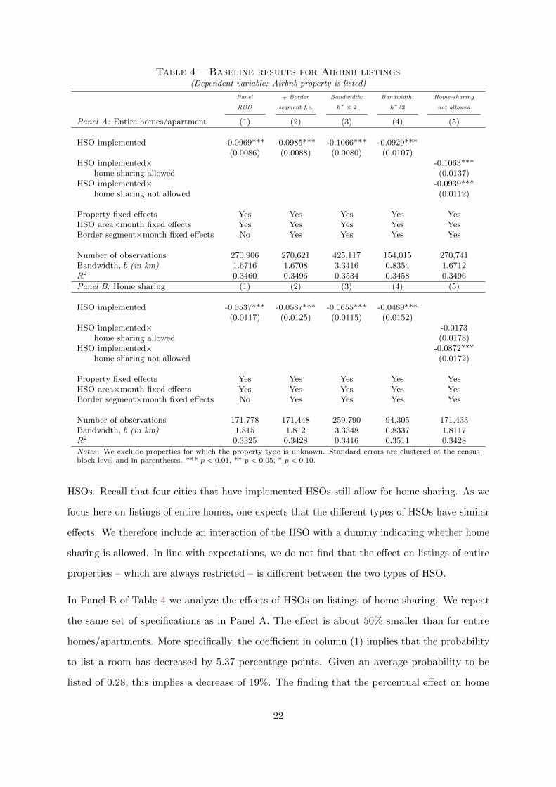
Table 4 – Baseline results for Airbnb listings(Dependent variable: Airbnb property is listed)

Panel + Border Bandwidth: Bandwidth: Home-sharing

RDD segment f.e. h∗ × 2 h∗/2 not allowed

Panel A: Entire homes/apartment (1) (2) (3) (4) (5)

HSO implemented -0.0969*** -0.0985*** -0.1066*** -0.0929***(0.0086) (0.0088) (0.0080) (0.0107)

HSO implemented× -0.1063***home sharing allowed (0.0137)

HSO implemented× -0.0939***home sharing not allowed (0.0112)

Property fixed effects Yes Yes Yes Yes YesHSO area×month fixed effects Yes Yes Yes Yes YesBorder segment×month fixed effects No Yes Yes Yes Yes

Number of observations 270,906 270,621 425,117 154,015 270,741Bandwidth, b (in km) 1.6716 1.6708 3.3416 0.8354 1.6712R2 0.3460 0.3496 0.3534 0.3458 0.3496

Panel B: Home sharing (1) (2) (3) (4) (5)

HSO implemented -0.0537*** -0.0587*** -0.0655*** -0.0489***(0.0117) (0.0125) (0.0115) (0.0152)

HSO implemented× -0.0173home sharing allowed (0.0178)


Property fixed effects Yes Yes Yes Yes YesHSO area×month fixed effects Yes Yes Yes Yes YesBorder segment×month fixed effects No Yes Yes Yes Yes


Notes: We exclude properties for which the property type is unknown. Standard errors are clustered at the censusblock level and in parentheses. *** p < 0.01, ** p < 0.05, * p < 0.10.

HSOs. Recall that four cities that have implemented HSOs still allow for home sharing. As we

focus here on listings of entire homes, one expects that the different types of HSOs have similar

effects. We therefore include an interaction of the HSO with a dummy indicating whether home

sharing is allowed. In line with expectations, we do not find that the effect on listings of entire

properties – which are always restricted – is different between the two types of HSO.

In Panel B of Table 4 we analyze the effects of HSOs on listings of home sharing. We repeat

the same set of specifications as in Panel A. The effect is about 50% smaller than for entire

homes/apartments. More specifically, the coefficient in column (1) implies that the probability

to list a room has decreased by 5.37 percentage points. Given an average probability to be

listed of 0.28, this implies a decrease of 19%. The finding that the percentual effect on home

22

sharing is smaller makes sense as some cities do not completely forbid home sharing (e.g. Santa

Monica). If we include border segment fixed effects (column (2)) or change the bandwidth

(columns (3) and (4)), this leaves the results essentially unaffected. In column (5) we again

include an interaction of the HSO with a dummy indicating whether home sharing is allowed.

As one expects, we do not find that home sharing listings have been reduced in areas where

home sharing is still allowed, whereas home sharing listings have been substantially reduced in

areas where short-term renting is completely banned, with a percentage point reduction that is

about the same as for entire homes/apartments. We think this provides strong evidence that

the changes in listings are really related to the implementation of HSOs.

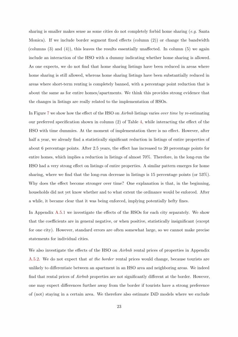
In Figure 7 we show how the effect of the HSO on Airbnb listings varies over time by re-estimating

our preferred specification shown in column (2) of Table 4, while interacting the effect of the

HSO with time dummies. At the moment of implementation there is no effect. However, after

half a year, we already find a statistically significant reduction in listings of entire properties of

about 6 percentage points. After 2.5 years, the effect has increased to 20 percentage points for

entire homes, which implies a reduction in listings of almost 70%. Therefore, in the long-run the

HSO had a very strong effect on listings of entire properties. A similar pattern emerges for home

sharing, where we find that the long-run decrease in listings is 15 percentage points (or 53%).

Why does the effect become stronger over time? One explanation is that, in the beginning,

households did not yet know whether and to what extent the ordinance would be enforced. After

a while, it became clear that it was being enforced, implying potentially hefty fines.

In Appendix A.5.1 we investigate the effects of the HSOs for each city separately. We show

that the coefficients are in general negative, or when positive, statistically insignificant (except

for one city). However, standard errors are often somewhat large, so we cannot make precise

statements for individual cities.

We also investigate the effects of the HSO on Airbnb rental prices of properties in Appendix

A.5.2. We do not expect that at the border rental prices would change, because tourists are

unlikely to differentiate between an apartment in an HSO area and neighboring areas. We indeed

find that rental prices of Airbnb properties are not significantly different at the border. However,

one may expect differences further away from the border if tourists have a strong preference

of (not) staying in a certain area. We therefore also estimate DiD models where we exclude

23

Figure 7 – The effect of the HSO on Airbnb listings over timeNotes: The optimal bandwidth b∗ = 1.6692 for ‘entire properties’ and h∗ = 1.8120 for ‘home sharing’. The dashed linesdenote the 95% confidence bands.

properties close to HSO borders (<2.5km). Still, we do not find any effect of HSOs on Airbnb

rental prices. These results are in line with the belief that the market for short-term rentals

is highly competitive: restrictions on short-term rental supply by HSOs (as well as additional

Transient Occupancy taxes) do not impact the spatial equilibrium of rental Airbnb prices.

We also investigate the effects of HSOs on the number of formally registered traveler accommo-

dation in Appendix A.5.3, using data from the County Business Patterns. Because we have data

on only a few years and the data is only available at the zipcode level, the results are imprecise.

However, the point estimates seem to point towards a sizeable 10% increase in the number of

formal traveler accommodations. Hence, we interpret this as suggestive evidence that HSOs

have led to an increase in formal accommodation.

6.2 HSOs and house prices

We have seen that the HSO strongly reduces the probability of using a property for short-term

renting. We expect that this will have a negative effect on house prices. In Table 5 we report

the results. Because house prices usually adjust only slowly, we exclude transactions occurring

within one year of implementation of the HSO.24 We start with a Panel RDD, including census

block and HSO areas×month fixed effects, as outlined above. The results in column (1) indicate

24We test later whether anticipation and adjustment effects are important.

24

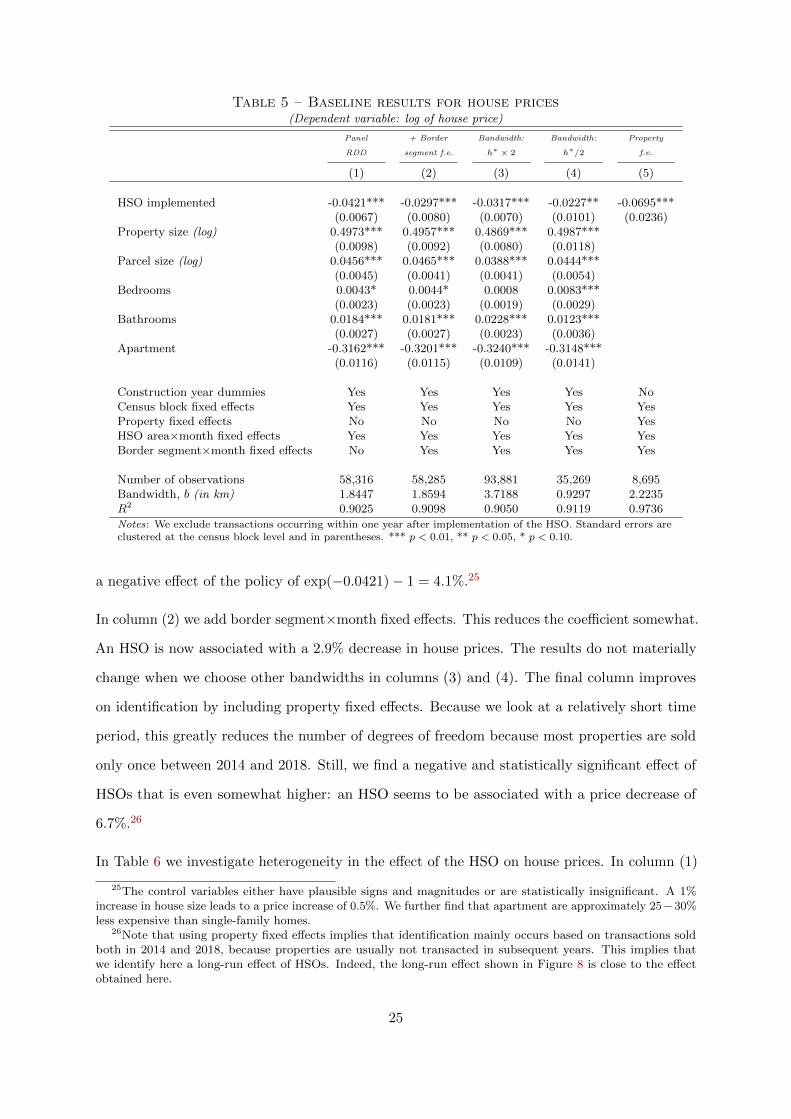
Table 5 – Baseline results for house prices(Dependent variable: log of house price)

Panel + Border Bandwidth: Bandwidth: Property

RDD segment f.e. h∗ × 2 h∗/2 f.e.

(1) (2) (3) (4) (5)

HSO implemented -0.0421*** -0.0297*** -0.0317*** -0.0227** -0.0695***(0.0067) (0.0080) (0.0070) (0.0101) (0.0236)

Property size (log) 0.4973*** 0.4957*** 0.4869*** 0.4987***(0.0098) (0.0092) (0.0080) (0.0118)

Parcel size (log) 0.0456*** 0.0465*** 0.0388*** 0.0444***(0.0045) (0.0041) (0.0041) (0.0054)

Bedrooms 0.0043* 0.0044* 0.0008 0.0083***(0.0023) (0.0023) (0.0019) (0.0029)

Bathrooms 0.0184*** 0.0181*** 0.0228*** 0.0123***(0.0027) (0.0027) (0.0023) (0.0036)

Apartment -0.3162*** -0.3201*** -0.3240*** -0.3148***(0.0116) (0.0115) (0.0109) (0.0141)

Construction year dummies Yes Yes Yes Yes NoCensus block fixed effects Yes Yes Yes Yes YesProperty fixed effects No No No No YesHSO area×month fixed effects Yes Yes Yes Yes YesBorder segment×month fixed effects No Yes Yes Yes Yes


Notes: We exclude transactions occurring within one year after implementation of the HSO. Standard errors areclustered at the census block level and in parentheses. *** p < 0.01, ** p < 0.05, * p < 0.10.

a negative effect of the policy of exp(−0.0421)− 1 = 4.1%.25

In column (2) we add border segment×month fixed effects. This reduces the coefficient somewhat.

An HSO is now associated with a 2.9% decrease in house prices. The results do not materially

change when we choose other bandwidths in columns (3) and (4). The final column improves

on identification by including property fixed effects. Because we look at a relatively short time

period, this greatly reduces the number of degrees of freedom because most properties are sold

only once between 2014 and 2018. Still, we find a negative and statistically significant effect of

HSOs that is even somewhat higher: an HSO seems to be associated with a price decrease of

6.7%.26

In Table 6 we investigate heterogeneity in the effect of the HSO on house prices. In column (1)

25The control variables either have plausible signs and magnitudes or are statistically insignificant. A 1%increase in house size leads to a price increase of 0.5%. We further find that apartment are approximately 25−30%less expensive than single-family homes.

26Note that using property fixed effects implies that identification mainly occurs based on transactions soldboth in 2014 and 2018, because properties are usually not transacted in subsequent years. This implies thatwe identify here a long-run effect of HSOs. Indeed, the long-run effect shown in Figure 8 is close to the effectobtained here.

25

Table 6 – HSOs and house prices: heterogeneity(Dependent variable: log of house price)

Distance Tourist Home sharing House type External

to beach pictures not allowed interactions effect

(1) (2) (3) (4) (5)

HSO implemented -0.0422*** -0.0229*** -0.0326***(0.0130) (0.0087) (0.0085)

HSO implemented× 0.0071distance to beach (log) (0.0056)

HSO implemented× -0.0104*pictures <200m (std) (0.0055)

HSO implemented× -0.0335***home sharing allowed (0.0116)


HSO implemented×single-family -0.0239**(0.0101)

HSO implemented×apartment -0.0346***(0.0097)

Share of HSO area 0-200m× 0.0223outside HSO area (0.0497)

Share of HSO area 200-500m× -0.0415outside HSO area (0.0342)

Property characteristics Yes Yes Yes Yes YesCensus block fixed effects Yes Yes Yes Yes YesHSO area×month fixed effects Yes Yes Yes Yes YesBorder segment×month fixed effects No Yes Yes Yes Yes


Notes: We exclude transactions occurring within one year after implementation of the HSO. Standarderrors are clustered at the census block level and in parentheses. *** p < 0.01, ** p < 0.05, * p < 0.10.

we first investigate whether HSOs have stronger effects in places where tourist demand is high.

As a first proxy for ‘touristy places’ we use distance to the beach. In column (1) we show that

the interaction effect of HSO with beach distance is not statistically significant at conventional

levels. However, its point estimate indicates that the effect of HSOs reduces by almost 0.5

percentage points, when the distance to the beach doubles (ln 2× 0.0071). Distance to the beach

is likely a very noisy proxy for touristy places, as places like Hollywood and Downtown LA are

far from the beach. This is supported if we focus on beach cities (e.g. Santa Monica): distance

to the beach appears to be important. Hence, we like to use a tourist measure which has more

general applicability.

We therefore use additional information on geocoded pictures by tourists. We count the number

of pictures within 200m and standardize this variable into an index with zero mean and unit

26

standard deviation. Column (2) shows that HSOs have a stronger effect in places with high

tourist demand. A standard deviation increase in tourist pictures implies that the negative effect

of HSOs is 1% stronger. In other words, restricting STRs in areas with strong tourist demand

has more severe repercussions for the housing market.

Column (3) tests whether HSOs that allow for home sharing have weaker price effects. This

appears not to be the case: the price effect for HSOs that allows for home sharing is not

statistically significantly different from the effect of HSOs in areas that do not allow for this.

In column (4) of Table 6 we include an interaction term with housing type. If local negative

externalities of Airbnb listings (e.g., noise) within buildings are important, we might expect to

see that prices of apartments have decreased less due to the HSO. This is not what we find. If

anything, the effect of the HSO is slightly stronger for apartments. However, the difference in

the effects for apartments and single-family homes is not statistically significant.

Column (5) investigates to what extent negative external effects related to tourism that spread

out to other areas play a role. Recall that theory indicates that an HSO has a negative effect

on house prices, because of a decrease in short-rental demand, but a supposedly positive effect

because of a reduction in negative tourist externalities. It is possible that reductions in tourism

within the HSO border also reduce negative effects of tourism across the border, potentially

increasing prices across borders. To investigate this, we calculate the share of land within 200m

and between 200 and 500m, just outside HSO areas. If there are negative external effects of

Airbnb, one expects to see price increases close to the HSO borders, because of a reduction in

those negative externalities. We do not find evidence for this.27 Furthermore, the main effect

related to HSOs is about the same as in the baseline specification. Overall, this implies that

negative external effects of tourism, if present, do not spread out to adjacent area and are

unlikely to be very large.

In Appendix A.5.1, we investigate heterogeneity between different cities in Los Angeles County

by estimating separate effects for each city. We exclude cities for which there are a limited

number (<100) of transactions after implementation of the HSO (e.g. in Pasadena, Calabasas)

or when there are fewer than 1000 transactions in or near the HSO area over the whole period

27We play around with different thresholds and including different rings, but the conclusion that externaleffects of Airbnb into adjacent areas are absent is unaffected.

27

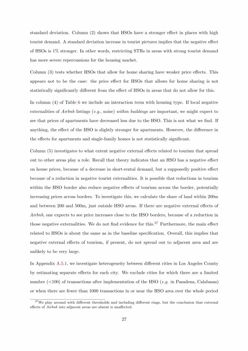
Figure 8 – The effect of the HSO on house prices over timeNotes: The optimal bandwidth b∗ = 1.8236. The dotted lines denote the 95% confidence bands.

(e.g. in Rolling Hills, Hermosa Beach). We are left with 8 HSO cities. The results are not always

precise. Nevertheless, we find that in 6 cities the effect is negative (and for two cities are highly

statistically significant). For most of the cities, these effects are not statistically different (at the

5% level) from the baseline estimate, which suggests that the variation in estimates between

cities might be entirely due to random variation and not due to more fundamental factors (e.g.,

the degree that the HSO is enforced).

A well-known issue with exploiting changes in house prices over time is that one has to take

anticipation effects into account. Anticipation effects may have been important as discussions on

the HSO predate implementation. Another issue is that it might have taken some time before

the HSO capitalized into house prices. We have tested this, with results shown in Figure 8. We

find that before implementation of the HSO there is no statistically significant price decrease,

hence there is no anticipation effect. At the moment of implementation we find that prices are

about 2.5% lower. The price effect becomes somewhat stronger over time, in line with Figure 7

in Section 6.1. 1.5 years after implementation the effect stabilizes at around 4.5%.

6.3 Airbnb listings and house prices

One could argue that the local average treatment effect of the HSO as estimated above does

not say much about the effect of Airbnb on house prices for specific neighborhoods, because

neighborhoods with a higher tourist accommodation demand are more strongly affected by the

28

ordinances (as implied by our analysis where the HSO effect varies with tourist demand). We

therefore estimate a ‘structural equation’ wherein we estimate the direct impact of the listings

rate on house prices. We determine the listings rate by calculating the number of listings relative

to the number of buildings within 200m of each property at each point in time.28 To deal

with endogeneity issues – omitted variable bias and potentially measurement error in listed or

approximated listings – we employ an instrumental variable approach using the HSO.

Table 7 reports the regression results for the two-stage Panel RDD.29 We observe in Table 7 that

the instrument is strong in all specifications.30 In Panel A we use imputed listings: the actual

listings that we impute for the months we do not have data. Panel B uses an alternative measure

using the date on the first and last review. The first-stage estimates, reported in Appendix A.5.5,

indicate that imputed and approximated listings rate have decreased by about 1.4 percentage

point, due to the HSO. This is in line with what we already established in the previous subsection:

the HSO has strongly reduced the number of Airbnb listings. The Kleibergen-Paap F -statistic

shows that the instrument is (very) strong in all specifications.

In column (1), Panel A, we find that the a 1 percentage point increase in the Airbnb listings

rate on property prices is 4.2%. In column (2) we include border segment×month fixed effects.

The effect reduces to 2.2%. A standard deviation increase in the listings rate is associated with

a 4.988× 0.0224 = 11.2% increase in prices, so the effect of Airbnb is substantial. The elasticity

for the average number of listings in the sample is 0.0224/1.1523 = 0.0194. When we only focus

on areas where an HSO is implemented the elasticity is 0.0206.31

Changing the bandwidth does not change the results much, as shown in columns (3) and (4) in

Panel A, although the effect is slightly lower if we focus on areas closer to the borders. When

we include property fixed effects (column (5)), the marginal effect is somewhat higher. A 1

percentage point increase in the listings rate is then associated with a price increase of 4.2%.

In Panel B we use a somewhat different proxy for Airbnb intensity, by approximating listings

28We take into account entire properties as well as home sharing. We use the threshold of 200m because thelocations of listings are known up to 200m.

29We obtain the bandwidth from the first stage: the regression of the listings rate on the dummy indicatingwhether an HSO is implemented.

30The first-stage F -statistic is above the rule-of-thumb value of 10 in all specifications but the last one wherewe include property fixed effects.

31These estimates are of a similar order of magnitude as Barron et al. (2018), who use a completely differentidentification strategy.

29

Table 7 – Airbnb listings and house prices: 2SLS estimates(Dependent variable: log of house price)



Panel A: Imputed listings (1) (2) (3) (4) (5)

Listings rate <200m (imputed) 0.0423*** 0.0224*** 0.0282*** 0.0159*** 0.0416**(0.0114) (0.0063) (0.0067) (0.0056) (0.0189)

Property characteristics Yes Yes Yes Yes NoCensus block fixed effects Yes Yes Yes Yes YesProperty fixed effects No No No No YesHSO area×month fixed effects Yes Yes Yes Yes YesBorder segment×month fixed effects No Yes Yes Yes Yes

Number of observations 89,424 89,362 150,245 55,517 16,282Bandwidth, b (in km) 3.4500 3.4642 6.9284 1.7321 4.3599Kleibergen-Paap F -statistic 17.45 28.68 34.37 18.27 9.394

Panel B: Approximated listings (1) (2) (3) (4) (5)

Listings rate <200m (approximated) 0.0414*** 0.0197*** 0.0244*** 0.0153*** 0.0269***(0.0095) (0.0053) (0.0057) (0.0051) (0.0096)


Number of observations 88,949 88,757 149,215 55,199 16,344Bandwidth, b (in km) 3.4219 3.4310 6.8620 1.7155 4.3712Kleibergen-Paap F -statistic 29.36 46.88 48.27 34.85 32.14

Notes: We exclude transactions occurring within one year after implementation of the HSO. The listings rateis instrumented by a dummy indicating whether an HSO has been instrumented. Standard errors are clusteredat the census block level and in parentheses. *** p < 0.01, ** p < 0.05, * p < 0.10.

using the first and last review and assuming that the property is continuously listed in between.

The results clearly show that this does not matter for the results. Our results are robust

regarding the proxy used for Airbnb listings in the vicinity. From hereon we therefore focus on

imputed listings.

6.4 Placebo checks and sensitivity

It is important to show the robustness of our results. In this subsection we will show some

‘placebo’-estimates and summarize the most important robustness checks.

In Table 8 we estimate regressions where we consider placebo HSOs for other areas. Panel A

reports the results for the effects on listings, while Panel B investigates the effects on house

prices.32

32In Panel A, we exclude transactions in HSO areas. In Panel B we further exclude transactions within one

30

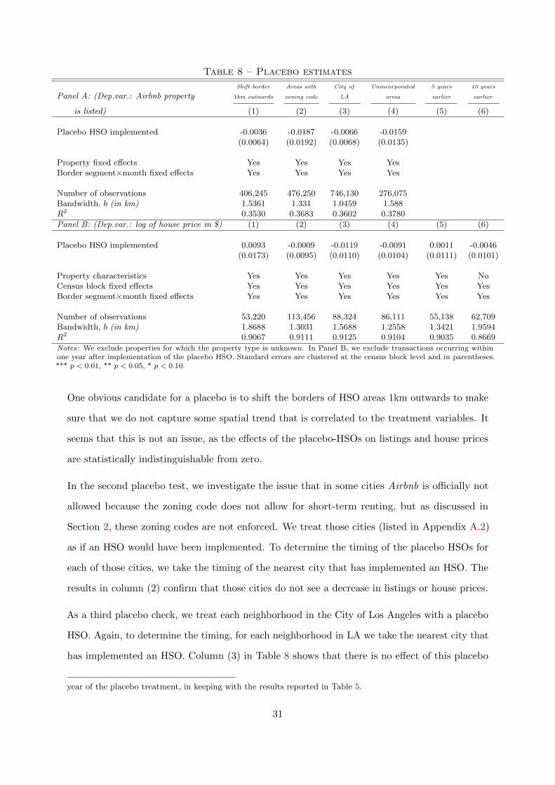
Table 8 – Placebo estimates

Shift border Areas with City of Unincorporated 5 years 10 years

Panel A: (Dep.var.: Airbnb property 1km outwards zoning code LA areas earlier earlier

is listed) (1) (2) (3) (4) (5) (6)

Placebo HSO implemented -0.0036 -0.0187 -0.0066 -0.0159(0.0064) (0.0192) (0.0068) (0.0135)

Property fixed effects Yes Yes Yes YesBorder segment×month fixed effects Yes Yes Yes Yes

Number of observations 406,245 476,250 746,130 276,075Bandwidth, b (in km) 1.5361 1.331 1.0459 1.588R2 0.3530 0.3683 0.3602 0.3780

Panel B: (Dep.var.: log of house price in $) (1) (2) (3) (4) (5) (6)

Placebo HSO implemented 0.0093 -0.0009 -0.0119 -0.0091 0.0011 -0.0046(0.0173) (0.0095) (0.0110) (0.0104) (0.0111) (0.0101)

Property characteristics Yes Yes Yes Yes Yes NoCensus block fixed effects Yes Yes Yes Yes Yes YesBorder segment×month fixed effects Yes Yes Yes Yes Yes Yes

Number of observations 53,220 113,456 88,324 86,111 55,138 62,709Bandwidth, b (in km) 1.8688 1.3031 1.5688 1.2558 1.3421 1.9594R2 0.9067 0.9111 0.9125 0.9104 0.9035 0.8669

Notes: We exclude properties for which the property type is unknown. In Panel B, we exclude transactions occurring withinone year after implementation of the placebo HSO. Standard errors are clustered at the census block level and in parentheses.*** p < 0.01, ** p < 0.05, * p < 0.10.

One obvious candidate for a placebo is to shift the borders of HSO areas 1km outwards to make

sure that we do not capture some spatial trend that is correlated to the treatment variables. It

seems that this is not an issue, as the effects of the placebo-HSOs on listings and house prices

are statistically indistinguishable from zero.

In the second placebo test, we investigate the issue that in some cities Airbnb is officially not

allowed because the zoning code does not allow for short-term renting, but as discussed in

Section 2, these zoning codes are not enforced. We treat those cities (listed in Appendix A.2)

as if an HSO would have been implemented. To determine the timing of the placebo HSOs for

each of those cities, we take the timing of the nearest city that has implemented an HSO. The

results in column (2) confirm that those cities do not see a decrease in listings or house prices.

As a third placebo check, we treat each neighborhood in the City of Los Angeles with a placebo

HSO. Again, to determine the timing, for each neighborhood in LA we take the nearest city that

has implemented an HSO. Column (3) in Table 8 shows that there is no effect of this placebo

year of the placebo treatment, in keeping with the results reported in Table 5.

31

HSO on listings or prices.

Column (4) continues by checking whether so-called ‘unincorporated’ areas, which have identical

regulation with respect to public goods and STRs, have seen changes in listings and prices.

To determine the timing of the placebo HSOs we again use the date of implementation of the

nearest HSO area. The coefficients clearly indicate that there is no effect of the placebo HSO.

In the final placebo checks we investigate whether we can detect any effect on housing prices

using data from exactly 5 and 10 years earlier (from 2009 until 2013 and from 2004 until

2008) and assume that the HSO would have been implemented exactly 5 or 10 years earlier.

Because Airbnb data is not available from before 2014, we cannot estimate this placebo test for

listings. For house prices, we again find that estimates are economically small and statistically

indistinguishable from zero.

Therefore, all placebo-estimates reported in Table 8 support the finding of a reduction in listings

and house prices due to implementation of the HSO is not a statistical artifact and unlikely the

result of a differential provision in the change of public goods or other regulation.

We subject this conclusion to a wide range of other sensitivity checks in Appendix A.5. More

specifically, in Appendix A.5.1 we report results where we estimate city-specific effects for the

effects of HSOs on listings and house prices, as discussed earlier. Appendix A.5.2 investigates

whether the HSO impacted rental prices of Airbnb. As mentioned earlier, we do not find

that this is the case. On the other hand, we find suggestive evidence that the number of

formal accommodations has increased in HSO areas (see Appendix A.5.3). In Appendix A.5.4

we investigate whether the standard errors change when taking into account cross-sectional

dependence. We show that standard errors are even somewhat smaller, although very comparable

to the baseline estimates where we cluster at the census block level. Appendix A.5.5 reports

first-stage results of the impact of the HSO on the listings rate. In Appendix A.5.6 we examine

robustness of our results if we (i) use distance to the border×year trends, (ii) include picture

density×year trends to control for changes in attractiveness of touristy areas, (iii) control for

trends in demographic variables, (iv) include straight border×year fixed effects to further address

any omitted variable bias, and (v) exclude outliers in the listings rate. The results are very

robust.

32

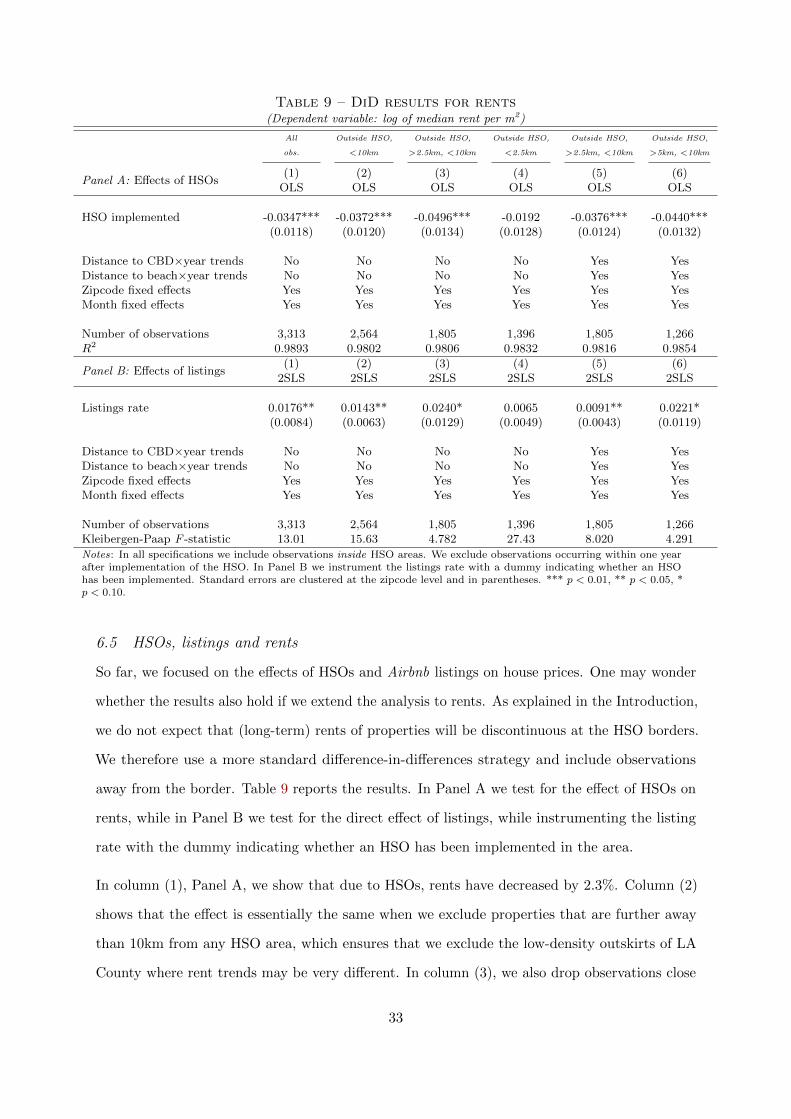
Table 9 – DiD results for rents(Dependent variable: log of median rent per m2)

All Outside HSO, Outside HSO, Outside HSO, Outside HSO, Outside HSO,

obs. <10km >2.5km, <10km <2.5km >2.5km, <10km >5km, <10km

Panel A: Effects of HSOs(1) (2) (3) (4) (5) (6)

OLS OLS OLS OLS OLS OLS

HSO implemented -0.0347*** -0.0372*** -0.0496*** -0.0192 -0.0376*** -0.0440***(0.0118) (0.0120) (0.0134) (0.0128) (0.0124) (0.0132)

Distance to CBD×year trends No No No No Yes YesDistance to beach×year trends No No No No Yes YesZipcode fixed effects Yes Yes Yes Yes Yes YesMonth fixed effects Yes Yes Yes Yes Yes Yes

Number of observations 3,313 2,564 1,805 1,396 1,805 1,266R2 0.9893 0.9802 0.9806 0.9832 0.9816 0.9854

Panel B: Effects of listings(1) (2) (3) (4) (5) (6)

2SLS 2SLS 2SLS 2SLS 2SLS 2SLS

Listings rate 0.0176** 0.0143** 0.0240* 0.0065 0.0091** 0.0221*(0.0084) (0.0063) (0.0129) (0.0049) (0.0043) (0.0119)


Number of observations 3,313 2,564 1,805 1,396 1,805 1,266Kleibergen-Paap F -statistic 13.01 15.63 4.782 27.43 8.020 4.291

Notes: In all specifications we include observations inside HSO areas. We exclude observations occurring within one yearafter implementation of the HSO. In Panel B we instrument the listings rate with a dummy indicating whether an HSOhas been implemented. Standard errors are clustered at the zipcode level and in parentheses. *** p < 0.01, ** p < 0.05, *p < 0.10.

6.5 HSOs, listings and rents

So far, we focused on the effects of HSOs and Airbnb listings on house prices. One may wonder

whether the results also hold if we extend the analysis to rents. As explained in the Introduction,

we do not expect that (long-term) rents of properties will be discontinuous at the HSO borders.

We therefore use a more standard difference-in-differences strategy and include observations

away from the border. Table 9 reports the results. In Panel A we test for the effect of HSOs on

rents, while in Panel B we test for the direct effect of listings, while instrumenting the listing

rate with the dummy indicating whether an HSO has been implemented in the area.

In column (1), Panel A, we show that due to HSOs, rents have decreased by 2.3%. Column (2)

shows that the effect is essentially the same when we exclude properties that are further away

than 10km from any HSO area, which ensures that we exclude the low-density outskirts of LA

County where rent trends may be very different. In column (3), we also drop observations close

33

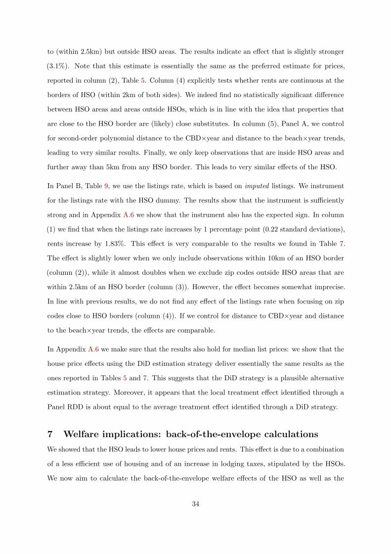
to (within 2.5km) but outside HSO areas. The results indicate an effect that is slightly stronger

(3.1%). Note that this estimate is essentially the same as the preferred estimate for prices,

reported in column (2), Table 5. Column (4) explicitly tests whether rents are continuous at the

borders of HSO (within 2km of both sides). We indeed find no statistically significant difference

between HSO areas and areas outside HSOs, which is in line with the idea that properties that

are close to the HSO border are (likely) close substitutes. In column (5), Panel A, we control

for second-order polynomial distance to the CBD×year and distance to the beach×year trends,

leading to very similar results. Finally, we only keep observations that are inside HSO areas and

further away than 5km from any HSO border. This leads to very similar effects of the HSO.

In Panel B, Table 9, we use the listings rate, which is based on imputed listings. We instrument

for the listings rate with the HSO dummy. The results show that the instrument is sufficiently

strong and in Appendix A.6 we show that the instrument also has the expected sign. In column

(1) we find that when the listings rate increases by 1 percentage point (0.22 standard deviations),

rents increase by 1.83%. This effect is very comparable to the results we found in Table 7.

The effect is slightly lower when we only include observations within 10km of an HSO border

(column (2)), while it almost doubles when we exclude zip codes outside HSO areas that are

within 2.5km of an HSO border (column (3)). However, the effect becomes somewhat imprecise.

In line with previous results, we do not find any effect of the listings rate when focusing on zip

codes close to HSO borders (column (4)). If we control for distance to CBD×year and distance

to the beach×year trends, the effects are comparable.

In Appendix A.6 we make sure that the results also hold for median list prices: we show that the

house price effects using the DiD estimation strategy deliver essentially the same results as the

ones reported in Tables 5 and 7. This suggests that the DiD strategy is a plausible alternative

estimation strategy. Moreover, it appears that the local treatment effect identified through a

Panel RDD is about equal to the average treatment effect identified through a DiD strategy.

7 Welfare implications: back-of-the-envelope calculations

We showed that the HSO leads to lower house prices and rents. This effect is due to a combination

of a less efficient use of housing and of an increase in lodging taxes, stipulated by the HSOs.

We now aim to calculate the back-of-the-envelope welfare effects of the HSO as well as the

34

distributional implications of the policy.

To be able to comment on the quantitative welfare effects of the HSO, we make several restrictive

assumptions. We refer to Appendix A.1 for more details on these assumptions, but we discuss

here the most important ones. First, welfare effects of tax avoidance are assumed to be absent.

This assumption is not too restrictive because the effects of tax avoidance by Airbnb suppliers

tend to be very small in LA, given the relatively low tax rates in California.33 Second, we

focus on locations far from the HSO border (which implies that we can avoid the complication

that rental households close to the border are not affected by the HSO). Third, we consider

the case where outside investors buy properties to list for short-term letting and assume that

the investors’ willingness to pay slightly exceeds the highest willingness to pay of incumbent

households. Fourth, we assume away distributional consequences of the HSO by assuming that

the marginal utility of income is constant.

Our preferred estimate in Table 5 indicates a 3% decrease in property values. We calculate

then the welfare effect using the average house price in HSO cities and obtain an annual welfare

loss of HSOs of about $680 per property. Given the substantial benefits of Airbnb, this seems

a reasonable number.34 The intuition for such a substantial loss is that the investors’ WTP

is much higher than the WTP of the marginal incumbent household being priced out of the

market.

In Table 10 we investigate the effects of Airbnb and HSOs on average property prices for LA

County as a whole and for specific areas, based on our estimates combined with descriptive

information on house prices and number of listings in these areas. To be more precise, we

evaluate the total effect of Airbnb using the listings rate in these areas as of 2018. We then

consider two counterfactual scenarios; one where no HSOs would have been implemented and

another where HSOs would apply to all areas in LA County. Of course, these calculations should

be interpreted with caution as we extrapolate a (local) average treatment effect to the wider

area of LA County. As the rent effect is essentially same as for prices (for which we provide

evidence in the previous subsection), we just report price effects here.

33Nevertheless, because tax avoidance of suppliers of Airbnb is likely present by the HSO, our decreases inwelfare because of efficiency losses are likely overestimates, but this does not have any consequence for thedistributional implications.

34In non-HSO areas this loss is slightly lower, because house prices are lower. The welfare loss of HSOs wouldbe about $610 a year in these areas if HSOs would have been implemented.

35

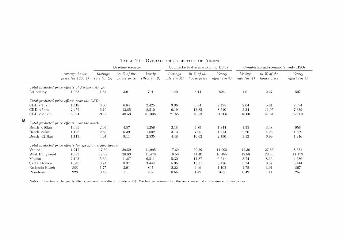
Table 10 – Overall price effects of Airbnb

Baseline scenario Counterfactual scenario 1: no HSOs Counterfactual scenario 2: only HSOs

Average house Listings in % of the Yearly Listings in % of the Yearly Listings in % of the Yearlyprice (in 1000 $) rate (in %) house price effect (in $) rate (in %) house price effect (in $) rate (in %) house price effect (in $)

Total predicted price effects of Airbnb listings:LA county 1,053 1.34 3.01 791 1.40 3.14 826 1.01 2.27 597

Total predicted price effects near the CBD:CBD <10km 1,418 3.06 6.84 2,425 3.06 6.84 2,425 2.64 5.91 2,094CBD <5km 2,457 6.19 13.85 8,510 6.19 13.85 8,510 5.34 11.95 7,339CBD <2.5km 5,054 21.68 48.53 61,306 21.68 48.53 61,306 18.60 41.64 52,603

Total predicted price effects near the beach:Beach <10km 1,099 2.04 4.57 1,256 2.18 4.89 1,344 1.55 3.48 956Beach <5km 1,128 2.86 6.39 1,802 3.13 7.00 1,974 2.20 4.93 1,389Beach <2.5km 1,113 4.07 9.11 2,535 4.48 10.02 2,790 3.12 6.99 1,946

Total predicted price effects for specific neighborhoods:Venice 1,212 17.69 39.59 11,995 17.69 39.59 11,995 12.36 27.66 8,381West Hollywood 1,593 12.88 28.83 11,479 18.50 41.40 16,485 12.88 28.83 11,479Malibu 2,193 5.30 11.87 6,511 5.30 11.87 6,511 3.74 8.36 4,586Santa Monica 1,645 3.74 8.37 3,444 5.95 13.31 5,476 3.74 8.37 3,444Redondo Beach 888 1.75 3.91 867 2.22 4.96 1,102 1.75 3.91 867Pasadena 928 0.49 1.11 257 0.66 1.49 345 0.49 1.11 257

Notes: To estimate the yearly effects, we assume a discount rate of 2%. We further assume that the rents are equal to discounted house prices.

36

Our estimates imply that the gains of Airbnb for LA County as a whole are quite modest (3.0%).

This is only true because many areas in LA counties have a low listings rate. When we focus

on areas within 5km of Los Angeles’s CBD, the house price effect would be 13.9%, which is

substantial. One may wonder whether these effects are realistic. It appears that house prices

within 5km of the CBD have increased by more than 40% in the last 10 years, so it seems that

these effects are possible. Given the high listings rate near the CBD, within 2.5km, the price

increase amount to almost 50%. Of course, we should take this prediction with a pinch of salt,

because we extrapolate a linear effect to large non-marginal changes in the listings rate. We

also consider the effects in beach towns. Within 2.5km, the price increase due to Airbnb has

been 9.1%. If we concentrate on specific cities and neighborhoods, the price effects of Airbnb do

vary substantially. In one of the most popular LA neighborhoods – Venice – the price increase is

almost 40%. On the other hand, in Pasadena (which is about 15km from Downtown LA), the

effects of Airbnb are negligible.

Let us consider the two counterfactual scenarios. First, we consider that all HSOs are abandoned.

Within 2.5km of a beach, this implies that the listings rate and house prices increase by

respectively 10% and 1%. For Santa Monica, which is well known for its strict HSO, the listings

rate would increase by 60% and the house price by almost 5%, which is substantial. For locations

near the CBD, abandoning HSOs does not imply changes in property values, because no areas

within the CBD are targeted by HSOs.

By contrast, if all incorporated cities would implement HSOs this has implications for prices

near the CBD. Within 5km of the CBD, the listings rate would decrease by 14% and prices

by 1.9%. For Venice the listings rate would drop by 30% and the price by almost 12%. Hence,

HSOs are likely to have large effects in areas attractive to tourists.

Our results also indicate that in neighborhoods attractive to tourists, the distributional con-

sequences are grave: in popular areas, incumbent homeowners have benefited more than 7.5

thousand per year due to Airbnb, whereas renters likely lost a similar amount. Somewhat less

popular neighborhoods for Airbnb are Santa Monica and Malibu. Still, Airbnb has led to price

and rent increases of 3.4-6.5 thousand a year.

There are clear distributional implications of HSOs. Homeowners will lose from the HSO, as the

37

demand for housing will decrease. This effect is due to a combination of a less efficient use of

housing (because properties are not available for their most profitable use) and of an increase

in lodging taxes, stipulated by the HSOs. However, (long-term) renters tend to gain because

rents decrease. This offers a plausible explanation as to why cities around the world that have

heavily restricted STRs typically have a high share of renters. In particular, cities that have

heavily restricted STRs, including Berlin and Amsterdam, have a high share of renters and

apartments.35

8 Conclusions

We have seen a spectacular growth of online short-term housing rental platforms in recent years.

However, it is yet unknown how these platforms affect the housing market.

We exploit quasi-experimental variation in Airbnb listings to test the impact of short-term

rentals on house prices and rents. We focus on Los Angeles County, where 18 cities have

implemented Home Sharing Ordinances that restrict short-term rentals between 2014 and 2018.

Using microdata for house prices and listings, we apply a Spatial Panel Regression-Discontinuity

Design around the borders of those areas and exploit the differences in timing of the HSOs.

Home Sharing Ordinances reduce Airbnb listings by about 70%, and reduce house prices by 3%

on average. Using aggregate data and a difference-in-differences estimation strategy we find

essentially the same effects for rents.

On average, Airbnb has positive, but small, effects on property values in LA County (about 3%).

This makes sense because in large parts of this county, Airbnb is not so popular. However, in

areas attractive to tourists, where the Airbnb listings rates are quite high, the effects of Airbnb

are substantial. Within 5km of the CBD, for example, the increase in property values is almost

14%. In Venice, which is a popular tourist destination, Airbnb has increased property value by

35We have analyzed the conditional relationship between the share of renters and the probability to implementan HSO using data for 88 incorporated cities and two unincorporated places in the Los Angeles area. Slightlysurprisingly, for these data, there is no correlation between the share of renters and the introduction of theHSO, but as shown in Appendix A.7, when we condition on income per capita (and, less importantly, a rangeof demographic indicators), then there appears to be a strong effect of the share renters on the probabilityto implement an HSO: the results suggest that there is proportional relationship between these two variables.We perceive this result as suggestive only, as we do not have exogenous variation in the share of renters. Wealso gathered some data for 29 other US cities. We find again suggestive evidence that a majority of renters isassociated with more stringent Airbnb regulations using a sample of 29 major US cities. We use the maximumnumber of days per year allowed for short-term letting as an (inverse) measure of stringency. The maximumallowed number of rental days is 45 for cities with a majority of renters, while it is 246 for all other cities (thecorrelation between maximum allowed number of rental days and the share of renters is −0.25).

38

40%.

Our estimates imply that Airbnb regulation has stark distributional implications, because it

induces losses for homeowners, which are very substantial for homeowners who live in areas that

are popular for tourists. The opposite holds for households who typically rent, who can only

gain from regulation as it reduces rents.

Ignoring the distributional consequences, our results suggest that Airbnb regulation has a negative

effect on overall welfare, given the important proviso that tax avoidance by suppliers of Airbnb

listings is limited. To address current tax avoidance, it is plausible that the optimal policy is

not to regulate short-term rental platforms quantitatively, as is the dominant way of regulating

platforms, but by addressing tax avoidance. This is feasible. For example, for several cities in

the world, including San Francisco and Amsterdam, Airbnb agreed to collect an ad-valorem

tourist tax for the city (without revealing information about Airbnb hosts).

39

ReferencesAhlfeldt, G. & Kavetsos, G. (2014), ‘Form or Function? The Effect of New Sports Stadia on Property Prices in

London’, Journal of the Royal Statistical Society A 177(1), 169–190.

Ahlfeldt, G., Moller, K., Waights, S. & Wendland, N. (2016), ‘Game of Zones: The Economics of Conservation

Areas’, Economic Journal p. Forthcoming.

Airbnb (2016), Airbnb’s Economic Impact in Los Angeles in 2016, Technical report.

Airbnb (2017), Airbnb Fast Facts, Technical report.

Barron, K., Kung, E. & Proserpio, D. (2018), ‘The Sharing Economy and Housing Affordability’, Working paper .

Bayer, P., Ferreira, F. & McMillan, R. (2007), ‘A Unified Framework for Measuring Preferences for Schools and

Neighborhoods’, Journal of Political Economy 115(4), 588–638.

Black, S. (1999), ‘Do Better Schools Matter? Parental Valuation of Elementary Education’, Quarterly Journal of

Economics 114(2), 577–599.

Brueckner, J. (1990), ‘Growth Controls and Land Values in an Open City.’, Land Economics 66(3), 237–248.

Carlino, G. & Saiz, A. (2008), ‘Beautiful City: Leisure Amenities and Urban Growth.’, Federal Reserce Bank of

Philadelphia Working Paper 0822 .

CBRE (2017), Hosts with Multiple Units - A Key Driver of Airbnb Growth, Technical report.

City of Santa Monica (2017).

Conley, T. (1999), ‘GMM Estimation with Cross sectional Dependence’, Journal of Econometrics 92(1), 1–45.

Edelman, B., Luca, M. & Svirsky, D. (2014), ‘Racial Discrimination in the Sharing Economy: Evidence from a

Field Experiment’, American Economic Journal (forthcoming) .

Filippas, A. & Horton, J. (2018), ‘The Tragedy of your Upstairs Neighbors: When is the Home-Sharing Externality

Internalized?’, Mimeo, NYU Stern School of Business, .

Fishman, S. (2015), ‘Overview of Airbnb Law in San Francisco’.

Gaigne, C., Koster, H., Moizeau, F. & Thisse, J. (2018), ‘Who Lives Where in Cities? Amenities, Commuting,

and Income Sorting’, CEPR Discussion Paper 11958 .

Garcia-Lopez, M., Jofre-Monseny, J., Martınez-Mazza, R. & Segu, M. (2018), ‘Do Short-term Rental Platforms

Affect Rents? Evidence from Airbnb in Barcelona’, Working paper .

Glaeser, E., Gyourko, J. & Saks, R. (2005), ‘Why have Housing Prices Gone up?’, American Economic Review:

Papers and Proceedings 95(2), 329–333.

Glaeser, E. & Ward, B. (2009), ‘The Causes and Consequences of Land Use Regulation: Evidence from Greater

Boston’, Journal of Urban Economics 65(3), 265–278.

Green, R., Malpezzi, S. & Mayo, S. (2005), ‘Metropolitan-Specific Estimates of the Price Elasticity of Supply of

40

Housing, and their Sources’, American Economic Review 95(2), 334–339.

Gutierrez, J., Garcıa-Palomares, J. C., Romanillos, G. & Salas-Olmedo, M. H. (2017), ‘The Eruption of AirBnB in

Tourist Cities: Comparing Spatial Patterns of Hotels and Peer-to-Peer Accommodation in Barcelona’, Tourism

Management 62, 278–291.

Hilber, C. & Vermeulen, W. (2016), ‘The Impact of Supply Constraints on House Prices in England’, Economic

Journal 126(591), 358–405.

Horn, K. & Merante, M. (2017), ‘Is home sharing driving up rents? Evidence from Airbnb in Boston’, Journal of

Housing Economics 38, 14–24.

Ihlanfeldt, K. (2007), ‘The Effect of Land Use Regulation on Housing and Land Prices’, Journal of Urban

Economics 61(3), 420–435.

Imbens, G. & Kalyanaraman, K. (2012), ‘Optimal Bandwidth Choice for the Regression Discontinuity Estimator’,

Review of Economic Studies 79(3), 933–959.

Imbens, G. & Lemieux, T. (2008), ‘Regression Discontinuity Designs: A Guide to Practice’, Journal of Econometrics

142(2), 615–635.

Inside Airbnb (2017), ‘Los Angeles, http://insideairbnb.com/los-angeles/’.

Kakar, V., Franco, J., Voelz, J. & Wu, J. (2016), Effects of Host Race Information on Airbnb Listing Prices in

San Francisco Effects of Host Race Information on Airbnb Listing Prices in San Francisco.

Koster, H. & Rouwendal, J. (2017), ‘Historic Amenities and Housing Externalities: Evidence from the Netherlands’,

Economic Journal 127, F396–F420.

Koster, H., Van Ommeren, J. & Rietveld, P. (2012), ‘Bombs, Boundaries and Buildings: a Regression-discontinuity

Approach to Measure Costs of Housing Supply Restrictions’, Regional Science and Urban Economics 42(4), 631–

641.

Lagorio-Chafkin, C. (2010), ‘Brian Chesky, Joe Gebbia, and Nathan Blecharczyk, Founders of AirBnB’.

Lee, D. (2016), ‘How Airbnb Short-Term Rentals Exacerbate Los Angeles’s Affordable Housing Crisis: Analysis

and Policy Recommendations.’, Harvard Law & Policy Review 10(1), 229–253.

Lee, D. & Lemieux, T. (2010), ‘Regression Discontinuity Designs in Economics’, Journal of Economic Literature

48(2), 281–355.

Lieber, R. (2015), ‘New Worry for Home Buyers: A Party House Next Door’, New York Times (October 9, 2015).

McCrary, J. (2008), ‘Manipulation of the Running Variable in the Regression Discontinuity Design: A Density

Test’, Journal of Econometrics 142(2), 698–714.

Moulton, B. (1990), ‘An Illustration of a Pitfall in Estimating the Effects of Aggregate Variables on Micro Units’,

Review of Economics and Statistics 72(2), 334–338.

NYCC (2015), Airbnb in NYC Housing Report, Technical report, New York Communities for Change, New York

41

http://insideairbnb.com/los-angeles/

City.

O’Sullivan, F. (2016), ‘The City With the World’s Toughest Anti-Airbnb Laws’.

Samaan, R. (2015), Airbnb, Rising Rent, and the Housing Crisis in Los Angeles, Technical report, Los Angeles

Alliance for a New Economy.

Sheppard, S. & Udell, A. (2016), Do AirBnB Properties Affect House Prices?

Turner, M., Haughwout, A. & Van der Klaauw, W. (2014), ‘Land Use Regulation and Welfare’, Econometrica

82(4), 1341–1403.

Van der Borg, J., Camatti, N., Bertocchi, D. & Albarea, A. (2017), The Rise of the Sharing Economy in Tourism:

Exploring Airbnb Attributes for the Veneto Region.

Van Duijn, M. & Rouwendal, J. (2013), ‘Cultural Heritage and the Location Choice of Dutch Households in a

Residential Sorting Model’, Journal of Economic Geography 13(3), 473–500.

Wachsmuth, D. & Weisler, A. (2017), Airbnb and the Rent Gap: Gentrification Through the Sharing Economy.

Williams, L. (2016), ‘When Airbnb Rentals Turn into Nuisance Neighbours’, The Guardian (September 18, 2016).

Zervas, G., Proserpio, D. & Byers, J. (2017), ‘The Rise of the Sharing Economy: Estimating the Impact of Airbnb

on the Hotel Industry’, Journal of Marketing Research 54(5), 687–705.

42

Online Appendix

A.1 Theoretical welfare considerations

What are the effects of implementing an HSO on welfare? Let us assume that welfare effects are

captured by changes in house prices and rents, in line with a large urban economics literature (see

e.g. Brueckner 1990).36 To be able to comment on the quantitative welfare effects of the HSO,

we make the following assumptions. (i) All agents have a discount rate of 2% and (ii) the same

marginal utility of income. (iii) Welfare effects of tax avoidance are assumed to be absent.37 (iv)

The demand functions for housing are linear and the total housing stock is given.38 (v) We focus

on locations far from the HSO border. (vi) Home-ownership and renting are perfect substitutes.

(vii). We consider the case where outside investors buy properties to list on Airbnb and assume

that the investors’ WTP slightly exceeds the highest WTP of incumbent households.39

In Figure A1 we show the demand effects of the HSO. We have drawn housing supply H∗ and

the equilibrium quantity of STR listings. In the initial situation, in the absence of regulation,

the equilibrium quantity of STRs is given by HSTR and the units used for residential housing is

H∗ −HSTR. In Figure A1, the HSO implies that HSTR = 0, which means a reduction in the

total surplus equal to A-B-E-F. Per property, the reduction in surplus is E-F.

A.2 Data appendix

Below, in Table A1, we report the results of our data gathering endeavors. Ready-to-use data

on Home Sharing Ordinances is not available, so we have browsed the Internet and phoned local

officials to know whether the city has implemented an HSO. For each city we report whether is

has implemented an HSO, whether home sharing is permitted, whether a STR needs to register

at the municipality and whether officially STRs are not allowed according the residential zoning

code. Furthermore, we list the sources from which we get the information.

36The latter assumption can be derived from more primitive assumptions, including that markets are competitive,except for the housing market where homeowners own the land and have market power.

37Because tax avoidance of suppliers of Airbnb is likely present by the HSO, our decreases in welfare because ofefficiency losses are likely overestimates, but this does not have any consequence for the distributional implications.

38This assumption is not essential, as non-linear demand functions implied by our log-linear hedonic pricefunctions, provide almost identical welfare results.

39Note that when the investors’ WTP does not exceed the highest WTP of incumbent households, then ourwelfare estimates are overestimates. We believe, however, that the assumption is defensible. Note further thatbecause the proportion of STRs is small compared to the other houses, about 2.5% in our data, the slope of theinvestors’ demand function is essentially irrelevant.

A1

Figure A1 – Demand effects of HSOs

A.3 Bandwidth selection

We use the approach proposed by Imbens & Kalyanaraman (2012), who show that the optimal

bandwidth can be estimated as:

b∗ = CK ·

(σ2−(c) + σ2

+(c)

f(c)×((m

(2)+ − m

(2)− )2 + (r+ + r−)

))15

×N−15 , (A.1)

where the constant CK = 3.4375 and N is the number of observations. σ2− and σ2

+ are the

conditional variances of respectively `ikt or log pijt given di = c on both sides of the threshold

(indicated with ‘−’ and ‘+’). f(c) denotes the estimated density of di at c. m(2)− and m(2) are

estimates of the second derivatives of a function of the dependent variable on the distance to

the boundary di. r+ and r− are estimated regularization terms that correct for potential error

in the estimation of the curvature of m(d) on both sides of the threshold.

Because we exploit variation in prices and the HSO over time to determine the bandwidths,

we first demean the variables by month and property or census block fixed effects. In many

specifications we add additional covariates (e.g. housing characteristics). We then determine

the conditional variance of the dependent variable given all covariates and fixed effects at the

threshold, so σ2−(c | xikt, λi, θkt) and σ2

+(c | xikt, λi, θkt). Usually, adding covariates does not

affect the optimal bandwidth much (Imbens & Kalyanaraman 2012). Indeed, adding a wide

array of controls barely influences the optimal bandwidth in our specifications.

A2

Table A1 – Home sharing ordinances and STR regulations in LA county

Name of city Year and month HSO Home sharing Register STR not in Sourceof implementation not allowed STR zoning code

Agoura Hills 0 0 0 0 phone interviewAlhambra 0 0 0 0 phone interviewArcadia 2017 7 1 1 1 0 phone interviewArtesia 0 0 0 0 web searchAzusa 0 0 0 1 web searchBaldwin Park 0 0 0 1 phone interviewBell 0 0 0 1 web searchBell Gardens 0 0 0 1 web searchBellflower 0 0 1 0 phone interviewBeverly Hills 2014 9 1 1 1 0 web searchBradbury 0 0 0 1 web searchBurbank 2014 6 1 1 1 0 web searchCalabasas 2018 1 1 0 1 0 web searchCarson 0 0 0 1 phone interviewCerritos 2016 8 1 1 1 0 web searchClaremont 0 0 0 1 phone interviewCommerce 0 0 0 1 web searchCompton 0 0 1 0 web searchCovina 0 0 0 1 phone interviewCudahy 0 0 0 1 web searchCulver City 0 0 0 1 phone interviewDiamond Bar 0 0 0 1 web searchDowney 0 0 0 1 phone interviewDuarte 0 0 0 1 web searchEl Monte 0 0 0 1 phone interviewEl Segundo 0 1 0 0 web searchGardena 0 0 0 1 web searchGlendale 0 0 0 0 phone interviewGlendora 0 0 0 1 web searchHawaiian Gardens 0 0 0 0 web searchHawthorne 0 0 0 1 web searchHermosa Beach 2016 6 1 1 1 0 web searchHidden Hills 0 0 0 1 web searchHuntington Park 0 0 0 1 web searchIndustry 0 0 0 0 web searchInglewood 0 0 0 1 web searchIrwindale 0 0 0 1 web searchLa Canada Flintridge 0 0 0 1 web searchLa Habra Heights 0 0 0 1 web searchLa Mirada 0 1 0 0 web searchLa Puente 0 0 0 1 web searchLa Verne 0 0 0 1 web searchLakewood 0 0 0 0 web searchLancaster 0 0 0 1 web searchLawndale 2017 7 1 1 0 0 web searchLomita 0 0 0 0 web searchLong Beach 0 1 0 0 web searchLos Angeles 0 1 0 0 web searchLynwood 0 0 0 1 web searchMalibu 2016 10 0 0 1 0 web searchManhattan Beach 2015 6 1 1 1 0 web searchMaywood 2018 4 1 1 0 0 web searchMonrovia 0 1 0 0 web searchMontebello 0 0 0 1 web searchMonterey Park 0 0 0 1 web searchNorwalk 0 0 0 1 web searchPalmdale 0 0 0 1 web searchPalos Verdes Estates 2016 9 1 1 1 0 web search

A3

Table A1 – continuedName of city Year and month HSO Home sharing Register STR not in Source

of implementation not allowed STR zoning code

Paramount 0 0 0 1 web searchPasadena 2017 10 1 0 1 0 web searchPico Rivera 0 0 0 1 web searchPomona 0 0 0 1 web searchRancho Palos Verdes 2016 7 1 1 1 0 web searchRedondo Beach 2016 6 1 1 1 0 web searchRolling Hills 2016 12 1 1 1 0 web searchRolling Hills Estates 2016 12 1 1 1 0 web searchRosemead 0 0 0 1 web searchSan Dimas 0 0 0 1 phone interviewSan Fernando 0 0 0 0 phone interviewSan Gabriel 0 0 0 1 phone interviewSan Marino 0 0 0 1 web searchSanta Clarita 0 0 0 0 phone interviewSanta Fe Springs 0 0 0 0 web searchSanta Monica 2015 6 1 0 1 0 web searchSierra Madre 0 1 0 0 web searchSignal Hill 0 1 0 0 web searchSouth El Monte 0 0 0 1 web searchSouth Gate 0 1 0 0 web searchSouth Pasadena 0 0 0 1 phone interviewTemple City 0 0 0 1 phone interviewTorrance 2016 4 1 0 1 0 web searchVernon 0 1 0 0 web searchWalnut 0 0 0 1 web searchWest Covina 0 1 0 0 web searchWest Hollywood 2015 9 1 1 1 0 web searchWestlake Village 0 0 0 0 phone interviewWhittier 0 0 0 1 phone interviewUnincorporated 0 0 1 0 web search

Note: We obtain information from the internet from:• https://la.lawsoup.org/legal-guides/laws-by-topic/short-term-vacation-rentals/,• https://www.dailybreeze.com/2016/03/02/redondo-beach-becomes-latest-south-bay-city-to-crack-down-on-short-term-rentals/,• https://www.newportbeachca.gov/government/departments/finance/revenue-division/short-term-rentals,• https://la.curbed.com/2014/3/24/10126966/the-few-places-in-los-angeles-where-airbnbs-might-be-legal,• https://www.latimes.com/tn-blr-burbank-changes-housing-rules-20140628-story.html, https://beverlyhills.granicus.com/,• https://www.beverlyhills.org/cbhfiles/storage/files/5614863821749456971/ShortTermRentals-Enforcement.pdf,• https://www.pasadenastarnews.com/2017/07/08/new-rules-are-coming-for-la-airbnb-hosts-heres-what-the-city-is-planning/,• https://www.mykawartha.com/news-story/8796058-rolling-hills-unhappy-with-status-quo-on-short-term-rentals/,• https://www.rpvca.gov/DocumentCenter/View/8725/Agenda-Item-2_RPV_SR_2016_07_12_-Short-Term-Vac-Rentals?bidId=,• https://tbrnews.com/news/redondo_beach/why-redondo-beach-wants-to-get-rid-of-airbnb-in/,• https://www.lakewoodcity.org/civicax/filebank/blobdload.aspx?BlobID=27108,• https://www.cerritos.us/NEWS_INFO/news_press_releases/2016/september/rentals.php,• https://cerritos.granicus.com/,• https://www.huntingtonbeachca.gov/announcements/announcement.cfm?id=917,• https://qcode.us/codes/lawndale/revisions/1139-17.pdf,• https://www.lomita.com/cityhall/government/ccMeetings/minutes_2016-09-06.pdf,• https://www.longbeach.gov/press-releases/community-to-help-shape-plans-for-a-short-term-rental-ordinance/,• https://cityofmaywoodpark.com/wp-content/uploads/2015/09/2018-2-ORDINANCE-2018-short-term-rentals-bnbs.pdf,• https://sausalito.granicus.com/,• https://sireagendas.westcovina.org/sirepub/cache/2/0n1f34d04rmjm3ook0naprwr/27509409222018040358852.PDF,• https://ttc.lacounty.gov/othertaxes/docs/FAQs%20for%20Online%20Hosting%20Platform%20FINAL.pdf.”

A.4 Other graphical evidence

In this Appendix we review ancillary graphical evidence that supports the identifying assumptions

we make in our research design. In Appendix A.4.1 we first consider cross-sectional variation

in the listing probability and house prices around the borders of HSO areas. Appendix A.4.2

considers discontinuities in housing characteristics and Appendix A.4.3 investigates jumps in

A4

https://la.lawsoup.org/legal-guides/laws-by-topic/short-term-vacation-rentals/

https://www.dailybreeze.com/2016/03/02/redondo-beach-becomes-latest-south-bay-city-to-crack-down-on-short-term-rentals/

https://www.newportbeachca.gov/government/departments/finance/revenue-division/short-term-rentals

https://la.curbed.com/2014/3/24/10126966/the-few-places-in-los-angeles-where-airbnbs-might-be-legal

https://www.latimes.com/tn-blr-burbank-changes-housing-rules-20140628-story.html

https://beverlyhills.granicus.com/

https://www.beverlyhills.org/cbhfiles/storage/files/5614863821749456971/ShortTermRentals-Enforcement.pdf

https://www.pasadenastarnews.com/2017/07/08/new-rules-are-coming-for-la-airbnb-hosts-heres-what-the-city-is-planning/

https://www.mykawartha.com/news-story/8796058-rolling-hills-unhappy-with-status-quo-on-short-term-rentals/

https://www.rpvca.gov/DocumentCenter/View/8725/Agenda-Item-2_RPV_SR_2016_07_12_-Short-Term-Vac-Rentals?bidId=

https://tbrnews.com/news/redondo_beach/why-redondo-beach-wants-to-get-rid-of-airbnb-in/

https://www.lakewoodcity.org/civicax/filebank/blobdload.aspx?BlobID=27108

https://www.cerritos.us/NEWS_INFO/news_press_releases/2016/september/rentals.php

https://cerritos.granicus.com/

https://www.huntingtonbeachca.gov/announcements/announcement.cfm?id=917

https://qcode.us/codes/lawndale/revisions/1139-17.pdf

https://www.lomita.com/cityhall/government/ccMeetings/minutes_2016-09-06.pdf

https://www.longbeach.gov/press-releases/community-to-help-shape-plans-for-a-short-term-rental-ordinance/

https://cityofmaywoodpark.com/wp-content/uploads/2015/09/2018-2-ORDINANCE-2018-short-term-rentals-bnbs.pdf

https://sausalito.granicus.com/

https://sireagendas.westcovina.org/sirepub/cache/2/0n1f34d04rmjm3ook0naprwr/27509409222018040358852.PDF

https://ttc.lacounty.gov/othertaxes/docs/FAQs%20for%20Online%20Hosting%20Platform%20FINAL.pdf

(a) Airbnb listings, before HSO (b) Airbnb listings, after HSO

(c) House price, before HSO (d) House price, after HSO

Figure A2 – Variation near HSO borders before and after the HSONotes: Negative distances indicate areas outside HSO areas. The dots are conditional averages at every 200m interval. Weinclude HSO border×month fixed effects. The dotted lines denote 95% confidence intervals.

densities of key variables after the HSO has been implemented.

A.4.1 Cross-sectional differences in listings and prices

In Figure A2 we illustrate cross-sectional differences in listings and house prices before and after

the HSOs were implemented. In Figure A2a, we compare the probability of being listed before

a HSO was implemented on both sides of the border. It is clear that there was essentially no

difference between HSO areas and surrounding areas. However, after the HSO was implemented,

the probability of being listed is approximately 4 percentage points lower (see Figure A2b). Note

that this effect is somewhat stronger when focusing on listings of entire properties (in keeping

with the results reported in Figure 3).

In Figures A2c and A2d, we consider cross-sectional variation in house prices on both sides of the

border before and after implementation of the HSO. This exercise clearly illustrates the difficulty

of obtaining valid estimates for the effects of Airbnb on house prices using a cross-sectional

approach, as there is substantial variation in prices around the border. Moreover, there is a

discrete jump in house prices at the HSO border. This is not too surprising, as there may be

A5

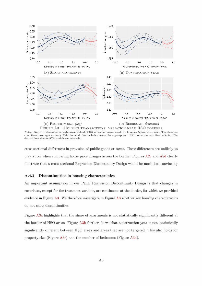
(a) Share apartments (b) Construction year

(c) Property size (log) (d) Bedrooms, demeaned

Figure A3 – Housing transactions: variation near HSO bordersNotes: Negative distances indicate areas outside HSO areas and areas inside HSO areas before treatment. The dots areconditional averages at every 200m interval. We include census block group and HSO border×month fixed effects. Thedotted lines denote 95% confidence intervals.

cross-sectional differences in provision of public goods or taxes. These differences are unlikely to

play a role when comparing house price changes across the border. Figures A2c and A2d clearly

illustrate that a cross-sectional Regression Discontinuity Design would be much less convincing.

A.4.2 Discontinuities in housing characteristics

An important assumption in our Panel Regression Discontinuity Design is that changes in

covariates, except for the treatment variable, are continuous at the border, for which we provided

evidence in Figure A3. We therefore investigate in Figure A3 whether key housing characteristics

do not show discontinuities.

Figure A3a highlights that the share of apartments is not statistically significantly different at

the border of HSO areas. Figure A3b further shows that construction year is not statistically

significantly different between HSO areas and areas that are not targeted. This also holds for

property size (Figure A3c) and the number of bedrooms (Figure A3d).

A6

(a) Change in density of listings (b) Change in density of transactions

Figure A4 – McCrary density testsNotes: We focus on observations before implementation of the HSO. Negative distances therefore indicate areas outside HSOareas. The dots are conditional densities at every 200m interval. The dotted lines denote 95% confidence intervals. On they-axis we ploy the difference in densities of McCrary’s density test between respectively listings and housing transactionsand the density of buildings.

A.4.3 Conditional McCrary tests

A test for discontinuities in densities of the running variable before the introduction of the HSO

might be informative, as a discontinuity might be indicative of unobserved housing or household

traits (e.g. different types of households sorting themselves into HSO areas) that are potentially

correlated with the treatment. However, this test should take into account the geography of the

area and borders of the areas, as discontinuities in listings or housing transactions are also due

that some areas border mountainous areas, parks or the sea.

We therefore estimate a two-step density test in the spirit of McCrary (2008). In the first step

we estimate the spatial distribution for buildings employing McCrary’s methodology. In the

second step we estimate this distribution for listings and for housing transactions respectively.

Our test is then the difference in the estimated densities between the second and first step.

Hence, a negative (or positive) density differential would indicate that there are fewer (or more)

listings/transactions than expected given the spatial distribution of buildings.

The results are reported in Figure A4. Figure A4a tests for the continuity of the density

differential of listings before an HSO was implemented. We find that there is no difference in

the density for listings at the HSO border. We repeat the same exercise, but now for housing

transactions in Figure A4b. This test indicates a discontinuity due to a higher density of

housing transactions just across the border in HSO areas. Note however that the discontinuity

is economically very small, so we do not consider this as a problem.

A7

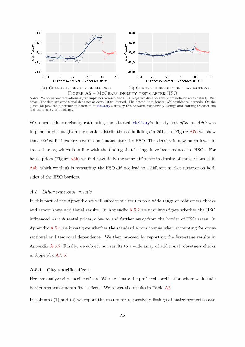
(a) Change in density of listings (b) Change in density of transactions

Figure A5 – McCrary density tests after HSONotes: We focus on observations before implementation of the HSO. Negative distances therefore indicate areas outside HSOareas. The dots are conditional densities at every 200m interval. The dotted lines denote 95% confidence intervals. On they-axis we ploy the difference in densities of McCrary’s density test between respectively listings and housing transactionsand the density of buildings.

We repeat this exercise by estimating the adapted McCrary’s density test after an HSO was

implemented, but given the spatial distribution of buildings in 2014. In Figure A5a we show

that Airbnb listings are now discontinuous after the HSO. The density is now much lower in

treated areas, which is in line with the finding that listings have been reduced to HSOs. For

house prices (Figure A5b) we find essentially the same difference in density of transactions as in

A4b, which we think is reassuring: the HSO did not lead to a different market turnover on both

sides of the HSO borders.

A.5 Other regression results

In this part of the Appendix we will subject our results to a wide range of robustness checks

and report some additional results. In Appendix A.5.2 we first investigate whether the HSO

influenced Airbnb rental prices, close to and further away from the border of HSO areas. In

Appendix A.5.4 we investigate whether the standard errors change when accounting for cross-

sectional and temporal dependence. We then proceed by reporting the first-stage results in

Appendix A.5.5. Finally, we subject our results to a wide array of additional robustness checks

in Appendix A.5.6.

A.5.1 City-specific effects

Here we analyze city-specific effects. We re-estimate the preferred specification where we include

border segment×month fixed effects. We report the results in Table A2.

In columns (1) and (2) we report the results for respectively listings of entire properties and

A8

Table A2 – City-specific effects for listings and prices(Dependent variable: log of house price in $)

(Dep.var.: (Dep.var.: (Dep.var.:

entire property is listed) home sharing is listed) log of house price in $)

(1) (2) (3)

HSO implemented×Arcadia -0.0999 -0.0933**(0.0626) (0.0465)

HSO implemented×Beverly Hills 0.0371(0.0293)

HSO implemented×Burbank -0.0710***(0.0274)

HSO implemented×Calabasas

HSO implemented×Cerritos -0.0340(0.0322)

HSO implemented×Hermosa Beach -0.1707*** -0.3095***(0.0556) (0.0768)

HSO implemented×Lawndale

HSO implemented×Manhattan Beach -0.0344 -0.0758* -0.0362(0.0315) (0.0423) (0.0301)

HSO implemented×Maywood

HSO implemented×Palos Verdes Estates

HSO implemented×Pasadena -0.0177 -0.0173(0.0396) (0.0454)

HSO implemented×Rancho Palos Verdes -0.2101 0.1133(0.1691) (0.1054)

HSO implemented×Rolling Hills

HSO implemented×Rolling Hills Estates

HSO implemented×Redondo Beach 0.0099 -0.0632 -0.0376(0.0532) (0.0626) (0.0336)

HSO implemented×Santa Monica -0.1713*** -0.0500*** -0.0236(0.0123) (0.0160) (0.0240)

HSO implemented×Torrance 0.0994** 0.0482 -0.0451**(0.0503) (0.0529) (0.0202)

HSO implemented×West-Hollywood -0.0909*** -0.0778*** 0.0234(0.0121) (0.0200) (0.0267)

Property characteristics No No YesProperty fixed effects Yes Yes NoCensus block fixed effects Yes Yes YesHSO area×month fixed effects Yes Yes YesBorder segment×month fixed effects No Yes Yes

Number of observations 264,605 163,969 33,680Bandwidth, b (in km) 1.6674 1.8255 1.9269R2 0.3496 0.3393 0.8574

Notes: In column (3), we exclude transactions occurring within one year after implementation of theHSO. Standard errors are clustered at the census block level and in parentheses. *** p < 0.01, **p < 0.05, * p < 0.10.

home sharing. We exclude observations in and near cities that have implemented HSOs before

the first observation in the data and cities for which we have fewer than 1000 listings over the

A9

whole sample period. Column (1) shows that the point estimates related to HSOs are almost

always negative and in three cases highly statistically significant. There is one exception: the

HSO seems to have had a positive effect on listings in Torrance. Column (2) also shows that most

coefficients are statistically significant and negative and comparable to the results in column (1).

In column (3) we focus on house prices. Again, we exclude observations for which we have fewer

than 1000 transactions in or near the respective city. This leaves us with 8 cities for which we

can estimate the effect. The results show that the effect is in most cases negative, although

somewhat imprecise. We find statistically significant effects for Burbank and Santa Monica. The

two positive point estimates observed in Beverly Hills and West-Hollywood are far from being

statistically significant.

A.5.2 HSOs and Airbnb short-term rental prices

Did HSOs have an impact on short-term rental prices of Airbnb properties? We explore this

in Table A3. These are hedonic price analyses using observations of properties that are listed

(in our dataset). We emphasize that spatial equilibrium theory indicates that at the border

short-term rental prices would not change, because tourists are unlikely to differentiate between

apartments in HSO areas and immediately adjacent areas and are therefore unlikely to be willing

to pay higher prices in areas that have implemented HSOs.

In column (1) we estimate the Panel RDD and do not find a statistically significant effect of an

HSO on Airbnb rental prices. This also holds if we include border segment×month fixed effects

in column (2) and changing the optimal bandwidth by 2 in columns (3) and (4). In column (5)

we include property fixed effects. In all cases the effect of an HSO on prices is economically

negligible and statistically insignificant.

We extend these results by using the same difference-in-differences approach as in Section 6.5.

In Table A4 we report the results. In column (1) we include all observations in LA County.

The effect of HSOs is small and statistically insignificant. This also holds if we only include

observations within 10km of any HSO border. In column (3), we exclude observations that are

close (<2km) within a border. Column (4) further controls for distance to CBD and distance to

the beach trends. The final column we exclude observations within 5km of an HSO border. All

results are economically small and far from statistically insignificant.

A10

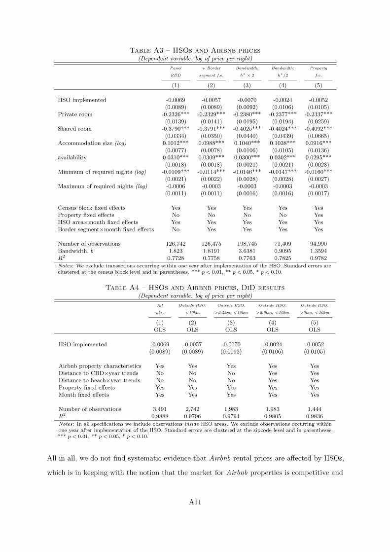
Table A3 – HSOs and Airbnb prices(Dependent variable: log of price per night)



(1) (2) (3) (4) (5)

HSO implemented -0.0069 -0.0057 -0.0070 -0.0024 -0.0052(0.0089) (0.0089) (0.0092) (0.0106) (0.0105)

Private room -0.2326*** -0.2329*** -0.2380*** -0.2377*** -0.2337***(0.0139) (0.0141) (0.0195) (0.0194) (0.0259)

Shared room -0.3790*** -0.3791*** -0.4025*** -0.4024*** -0.4092***(0.0334) (0.0350) (0.0440) (0.0439) (0.0665)

Accommodation size (log) 0.1012*** 0.0988*** 0.1040*** 0.1038*** 0.0916***(0.0077) (0.0078) (0.0106) (0.0105) (0.0136)

availability 0.0310*** 0.0309*** 0.0300*** 0.0302*** 0.0295***(0.0018) (0.0018) (0.0021) (0.0021) (0.0023)

Minimum of required nights (log) -0.0109*** -0.0114*** -0.0146*** -0.0147*** -0.0160***(0.0021) (0.0022) (0.0028) (0.0028) (0.0027)

Maximum of required nights (log) -0.0006 -0.0003 -0.0003 -0.0003 -0.0003(0.0011) (0.0011) (0.0016) (0.0016) (0.0017)

Census block fixed effects Yes Yes Yes Yes YesProperty fixed effects No No No No YesHSO area×month fixed effects Yes Yes Yes Yes YesBorder segment×month fixed effects No Yes Yes Yes Yes

Number of observations 126,742 126,475 198,745 71,409 94,990Bandwidth, b 1.823 1.8191 3.6381 0.9095 1.3594R2 0.7728 0.7758 0.7763 0.7825 0.9782

Notes: We exclude transactions occurring within one year after implementation of the HSO. Standard errors areclustered at the census block level and in parentheses. *** p < 0.01, ** p < 0.05, * p < 0.10.

Table A4 – HSOs and Airbnb prices, DiD results(Dependent variable: log of price per night)

All Outside HSO, Outside HSO, Outside HSO, Outside HSO,

obs. <10km >2.5km, <10km >2.5km, <10km >5km, <10km

(1) (2) (3) (4) (5)OLS OLS OLS OLS OLS

HSO implemented -0.0069 -0.0057 -0.0070 -0.0024 -0.0052(0.0089) (0.0089) (0.0092) (0.0106) (0.0105)

Airbnb property characteristics Yes Yes Yes Yes YesDistance to CBD×year trends No No No Yes YesDistance to beach×year trends No No No Yes YesProperty fixed effects Yes Yes Yes Yes YesMonth fixed effects Yes Yes Yes Yes Yes

Number of observations 3,491 2,742 1,983 1,983 1,444R2 0.9888 0.9796 0.9794 0.9805 0.9836

Notes: In all specifications we include observations inside HSO areas. We exclude observations occurring withinone year after implementation of the HSO. Standard errors are clustered at the zipcode level and in parentheses.*** p < 0.01, ** p < 0.05, * p < 0.10.

All in all, we do not find systematic evidence that Airbnb rental prices are affected by HSOs,

which is in keeping with the notion that the market for Airbnb properties is competitive and

A11

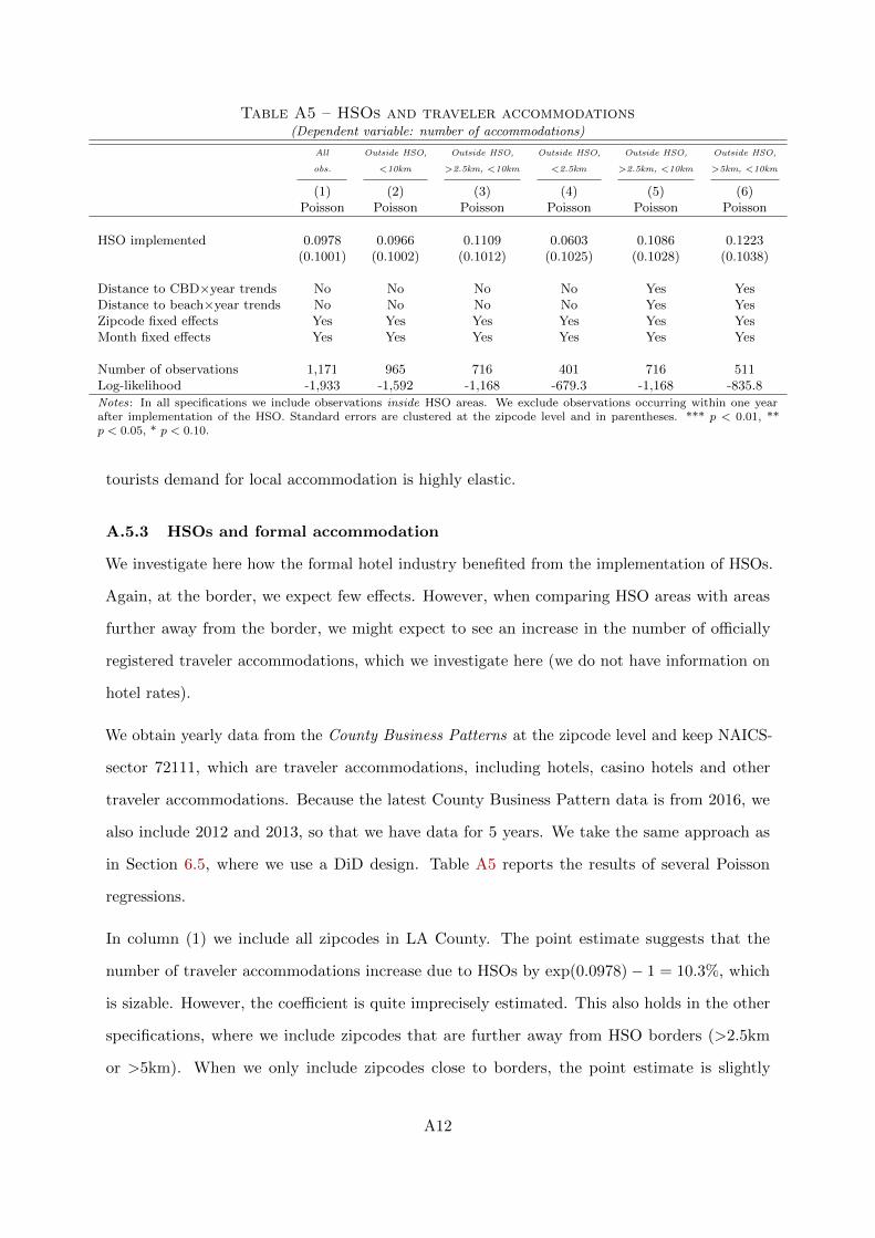
Table A5 – HSOs and traveler accommodations(Dependent variable: number of accommodations)



(1) (2) (3) (4) (5) (6)Poisson Poisson Poisson Poisson Poisson Poisson

HSO implemented 0.0978 0.0966 0.1109 0.0603 0.1086 0.1223(0.1001) (0.1002) (0.1012) (0.1025) (0.1028) (0.1038)


Number of observations 1,171 965 716 401 716 511Log-likelihood -1,933 -1,592 -1,168 -679.3 -1,168 -835.8

Notes: In all specifications we include observations inside HSO areas. We exclude observations occurring within one yearafter implementation of the HSO. Standard errors are clustered at the zipcode level and in parentheses. *** p < 0.01, **p < 0.05, * p < 0.10.

tourists demand for local accommodation is highly elastic.

A.5.3 HSOs and formal accommodation

We investigate here how the formal hotel industry benefited from the implementation of HSOs.

Again, at the border, we expect few effects. However, when comparing HSO areas with areas

further away from the border, we might expect to see an increase in the number of officially

registered traveler accommodations, which we investigate here (we do not have information on

hotel rates).

We obtain yearly data from the County Business Patterns at the zipcode level and keep NAICS-

sector 72111, which are traveler accommodations, including hotels, casino hotels and other

traveler accommodations. Because the latest County Business Pattern data is from 2016, we

also include 2012 and 2013, so that we have data for 5 years. We take the same approach as

in Section 6.5, where we use a DiD design. Table A5 reports the results of several Poisson

regressions.

In column (1) we include all zipcodes in LA County. The point estimate suggests that the

number of traveler accommodations increase due to HSOs by exp(0.0978)− 1 = 10.3%, which

is sizable. However, the coefficient is quite imprecisely estimated. This also holds in the other

specifications, where we include zipcodes that are further away from HSO borders (>2.5km

or >5km). When we only include zipcodes close to borders, the point estimate is slightly

A12

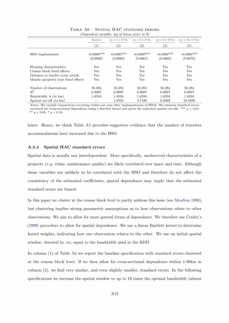
Table A6 – Spatial HAC standard errors(Dependent variable: log of house price in $)

Baseline sw = 1× b∗km sw = 2× b∗km sw = 5× b∗km sw = 10× b∗km

(1) (2) (3) (4) (5)

HSO implemented -0.0300*** -0.0300*** -0.0300*** -0.0300*** -0.0300***(0.0080) (0.0066) (0.0067) (0.0069) (0.0070)

Housing characteristics Yes Yes Yes Yes YesCensus block fixed effects Yes Yes Yes Yes YesDistance to border×year trends Yes Yes Yes Yes YesMonth×property type fixed effects Yes Yes Yes Yes Yes

Number of observations 58,284 58,284 58,284 58,284 58,284R2 0.9097 0.9097 0.9097 0.9097 0.9097Bandwidth, b (in km) 1.8594 1.8594 1.8594 1.8594 1.8594Spatial cut-off (in km) — 1.8594 3.7188 9.2969 18.5938

Notes: We exclude transactions occurring within one year after implementation of HSOs. We estimate standard errorscorrected for cross-sectional dependence using a Bartlett kernel and given the indicated spatial cut-offs. *** p < 0.01,** p < 0.05, * p < 0.10.

lower. Hence, we think Table A5 provides suggestive evidence that the number of travelers

accommodations have increased due to the HSO.

A.5.4 Spatial HAC standard errors

Spatial data is usually not interdependent. More specifically, unobserved characteristics of a

property (e.g. crime, maintenance quality) are likely correlated over space and time. Although

these variables are unlikely to be correlated with the HSO and therefore do not affect the

consistency of the estimated coefficients, spatial dependence may imply that the estimated

standard errors are biased.

In this paper we cluster at the census block level to partly address this issue (see Moulton 1990),

but clustering implies strong parametric assumptions as to how observations relate to other

observations. We aim to allow for more general forms of dependence. We therefore use Conley’s

(1999) procedure to allow for spatial dependence. We use a linear Bartlett kernel to determine

kernel weights, indicating how one observation relates to the other. We use an initial spatial

window, denoted by sw, equal to the bandwidth used in the RDD.

In column (1) of Table A6 we report the baseline specification with standard errors clustered

at the census block level. If we then allow for cross-sectional dependence within 1.86km in

column (2), we find very similar, and even slightly smaller, standard errors. In the following

specifications we increase the spatial window to up to 10 times the optimal bandwidth (almost

A13

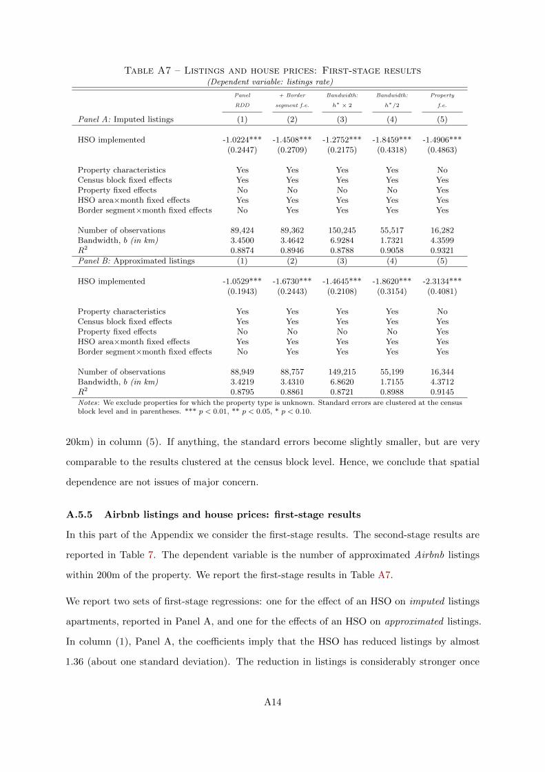
Table A7 – Listings and house prices: First-stage results(Dependent variable: listings rate)



Panel A: Imputed listings (1) (2) (3) (4) (5)

HSO implemented -1.0224*** -1.4508*** -1.2752*** -1.8459*** -1.4906***(0.2447) (0.2709) (0.2175) (0.4318) (0.4863)



Panel B: Approximated listings (1) (2) (3) (4) (5)

HSO implemented -1.0529*** -1.6730*** -1.4645*** -1.8620*** -2.3134***(0.1943) (0.2443) (0.2108) (0.3154) (0.4081)



Notes: We exclude properties for which the property type is unknown. Standard errors are clustered at the censusblock level and in parentheses. *** p < 0.01, ** p < 0.05, * p < 0.10.

20km) in column (5). If anything, the standard errors become slightly smaller, but are very

comparable to the results clustered at the census block level. Hence, we conclude that spatial

dependence are not issues of major concern.

A.5.5 Airbnb listings and house prices: first-stage results

In this part of the Appendix we consider the first-stage results. The second-stage results are

reported in Table 7. The dependent variable is the number of approximated Airbnb listings

within 200m of the property. We report the first-stage results in Table A7.

We report two sets of first-stage regressions: one for the effect of an HSO on imputed listings

apartments, reported in Panel A, and one for the effects of an HSO on approximated listings.

In column (1), Panel A, the coefficients imply that the HSO has reduced listings by almost

1.36 (about one standard deviation). The reduction in listings is considerably stronger once

A14

we control for border segment×month fixed effects. The HSO is associated with a reduction

in approximated listings 2.29. The first-stage coefficient becomes somewhat stronger for small

bandwidths (columns (3) and (4)). In column (5) we show that when excluding South Bay cities,

an HSO reduces listings by about 3, which is also found when we include property fixed effects in

column (6). The effects on imputed listings, reported in Panel B, Table 7, are very much similar.

A.5.6 Sensitivity analysis

Here, we subject our results to some addition range of robustness checks. We report the results

in Table A8. In Panel A we report the results that refer to the direct house price effects of the

HSO. Panels B and C focuses on the ‘structural equation’ where we regress prices on imputed

and approximated Airbnb listings, respectively, while instrumenting with the HSO.

In this paper we use a Panel RDD to identify the house price effects based on an optimal

bandwidth. As a sensitivity check instead of using a bandwidth we include a second-order

polynomial of distance to the nearest HSO border interacted by year, while including all

observations. In column (1) we see that this has limited repercussions for the results. If anything,

the effects are slightly stronger.

One may still be worried that the effects of Airbnb are partly determined by locational attrac-

tiveness. Column (2) aims to further alleviate these concerns by including flexible second-order

trends of pictures and year. The results are hardly affected.

In column (3) we match the transactions data to neighborhood characteristics (at the census

block group level). That is, we match each transaction to the log of population density, share of

blacks, Hispanics, and Asians, household compositions, the share of renters and the median age,

in the previous year. Given that the effects are then very similar, this suggests that the effect of

the HSOs (Airbnb) is predominantly due to a reduction (increase) in demand, rather than due

to changes in the neighborhood composition.

Column (4) further improves on identification by including straight border segment×year fixed

effects in spirit of Turner et al. (2014). The idea is that straight border segments are likely

uncorrelated to geographical features of a location, which may impact price trends (e.g. through

the propensity to build on the land). Because the average length of a straight border segment

is just below 50m, we cannot include border segment×month fixed effects, as this will lead to

A15

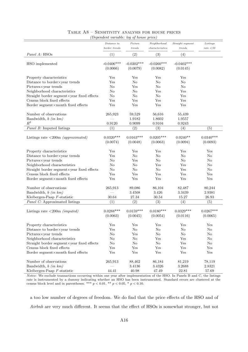
Table A8 – Sensitivity analysis for house prices(Dependent variable: log of house price)

Distance to Picture Neighborhood Straight segment Listings

border trends trends characteristics trends rate <50

Panel A: HSOs (1) (2) (3) (4)

HSO implemented -0.0406*** -0.0302*** -0.0260*** -0.0402***(0.0066) (0.0079) (0.0082) (0.0145)

Property characteristics Yes Yes Yes YesDistance to border×year trends Yes No No NoPictures×year trends No Yes No NoNeighborhood characteristics No No Yes YesStraight border segment×year fixed effects No No No YesCensus block fixed effects Yes Yes Yes YesBorder segment×month fixed effects Yes Yes Yes Yes

Number of observations 265,923 59,529 56,616 55,439Bandwidth, b (in km) — 1.9182 1.8602 1.9557R2 0.9120 0.9099 0.9104 0.9243

Panel B: Imputed listings (1) (2) (3) (4) (5)

Listings rate <200m (approximated) 0.0320*** 0.0163*** 0.0205*** 0.0240** 0.0340***(0.0074) (0.0048) (0.0063) (0.0094) (0.0093)

Property characteristics Yes Yes Yes Yes YesDistance to border×year trends Yes No No No NoPictures×year trends No Yes No No NoNeighborhood characteristics No No Yes Yes NoStraight border segment×year fixed effects No No No Yes NoCensus block fixed effects Yes Yes Yes Yes YesBorder segment×month fixed effects Yes Yes Yes Yes Yes

Number of observations 265,913 89,086 86,104 82,487 80,244Bandwidth, b (in km) — 3.4508 3.426 3.3439 2.9381Kleibergen-Paap F -statistic 30.64 27.34 30.54 15.27 26.93

Panel C: Approximated listings (1) (2) (3) (4) (5)

Listings rate <200m (imputed) 0.0288*** 0.0159*** 0.0180*** 0.0329*** 0.0267***(0.0063) (0.0045) (0.0054) (0.0116) (0.0065)

Property characteristics Yes Yes Yes Yes YesDistance to border×year trends Yes No No No NoPictures×year trends No Yes No No NoNeighborhood characteristics No No Yes Yes NoStraight border segment×year fixed effects No No No Yes NoCensus block fixed effects Yes Yes Yes Yes YesBorder segment×month fixed effects Yes Yes Yes Yes Yes

Number of observations 265,913 88,462 86,184 81,219 78,119Bandwidth, b (in km) — 3.4136 3.4326 3.2688 2.8321Kleibergen-Paap F -statistic 44.41 40.98 47.49 22.81 57.69

Notes: We exclude transactions occurring within one year after implementation of the HSO. In Panels B and C, the listingsrate is instrumented by a dummy indicating whether an HSO has been instrumented. Standard errors are clustered at thecensus block level and in parentheses. *** p < 0.01, ** p < 0.05, * p < 0.10.

a too low number of degrees of freedom. We do find that the price effects of the HSO and of

Airbnb are very much different. It seems that the effect of HSOs is somewhat stronger, but not

A16

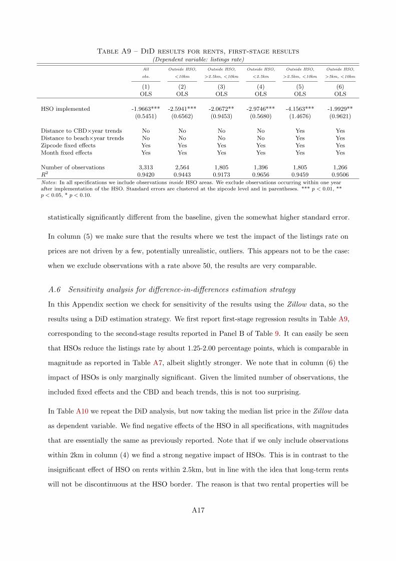
Table A9 – DiD results for rents, first-stage results(Dependent variable: listings rate)



(1) (2) (3) (4) (5) (6)OLS OLS OLS OLS OLS OLS

HSO implemented -1.9663*** -2.5941*** -2.0672** -2.9746*** -4.1563*** -1.9929**(0.5451) (0.6562) (0.9453) (0.5680) (1.4676) (0.9621)



Notes: In all specifications we include observations inside HSO areas. We exclude observations occurring within one yearafter implementation of the HSO. Standard errors are clustered at the zipcode level and in parentheses. *** p < 0.01, **p < 0.05, * p < 0.10.

statistically significantly different from the baseline, given the somewhat higher standard error.

In column (5) we make sure that the results where we test the impact of the listings rate on

prices are not driven by a few, potentially unrealistic, outliers. This appears not to be the case:

when we exclude observations with a rate above 50, the results are very comparable.

A.6 Sensitivity analysis for difference-in-differences estimation strategy

In this Appendix section we check for sensitivity of the results using the Zillow data, so the

results using a DiD estimation strategy. We first report first-stage regression results in Table A9,

corresponding to the second-stage results reported in Panel B of Table 9. It can easily be seen

that HSOs reduce the listings rate by about 1.25-2.00 percentage points, which is comparable in

magnitude as reported in Table A7, albeit slightly stronger. We note that in column (6) the

impact of HSOs is only marginally significant. Given the limited number of observations, the

included fixed effects and the CBD and beach trends, this is not too surprising.

In Table A10 we repeat the DiD analysis, but now taking the median list price in the Zillow data

as dependent variable. We find negative effects of the HSO in all specifications, with magnitudes

that are essentially the same as previously reported. Note that if we only include observations

within 2km in column (4) we find a strong negative impact of HSOs. This is in contrast to the

insignificant effect of HSO on rents within 2.5km, but in line with the idea that long-term rents

will not be discontinuous at the HSO border. The reason is that two rental properties will be

A17

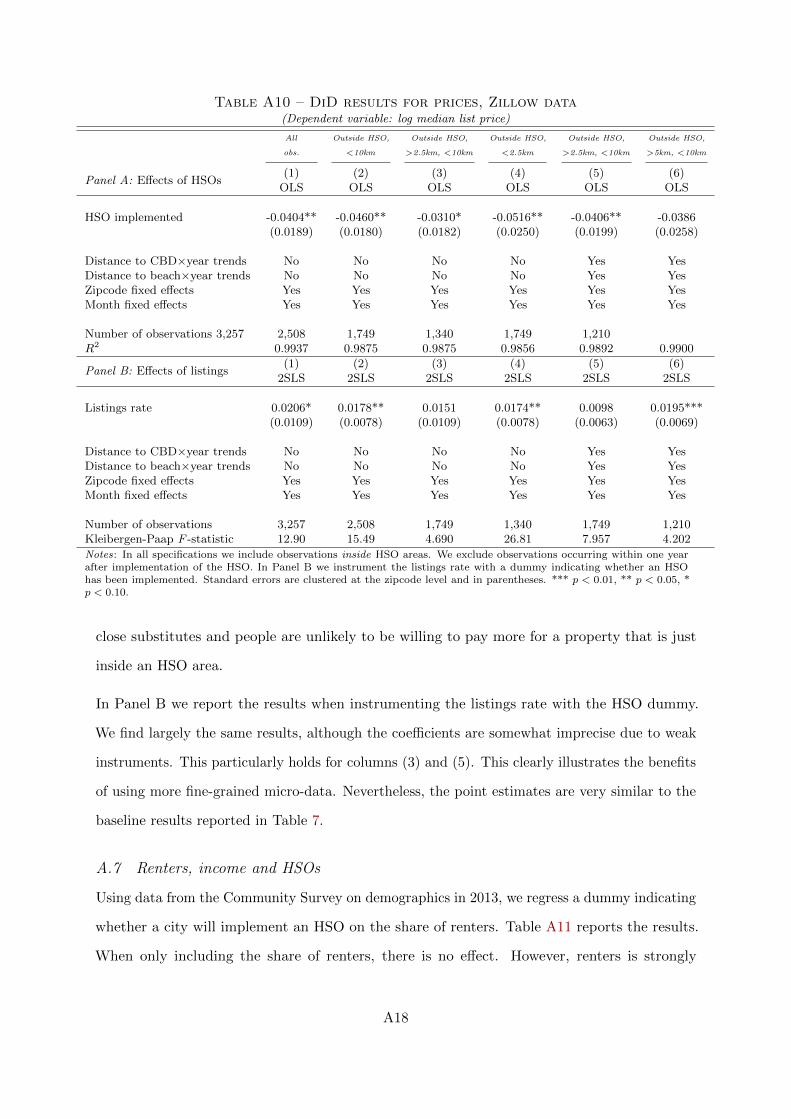
Table A10 – DiD results for prices, Zillow data(Dependent variable: log median list price)



Panel A: Effects of HSOs(1) (2) (3) (4) (5) (6)

OLS OLS OLS OLS OLS OLS

HSO implemented -0.0404** -0.0460** -0.0310* -0.0516** -0.0406** -0.0386(0.0189) (0.0180) (0.0182) (0.0250) (0.0199) (0.0258)



Panel B: Effects of listings(1) (2) (3) (4) (5) (6)

2SLS 2SLS 2SLS 2SLS 2SLS 2SLS

Listings rate 0.0206* 0.0178** 0.0151 0.0174** 0.0098 0.0195***(0.0109) (0.0078) (0.0109) (0.0078) (0.0063) (0.0069)


Number of observations 3,257 2,508 1,749 1,340 1,749 1,210Kleibergen-Paap F -statistic 12.90 15.49 4.690 26.81 7.957 4.202

Notes: In all specifications we include observations inside HSO areas. We exclude observations occurring within one yearafter implementation of the HSO. In Panel B we instrument the listings rate with a dummy indicating whether an HSOhas been implemented. Standard errors are clustered at the zipcode level and in parentheses. *** p < 0.01, ** p < 0.05, *p < 0.10.

close substitutes and people are unlikely to be willing to pay more for a property that is just

inside an HSO area.

In Panel B we report the results when instrumenting the listings rate with the HSO dummy.

We find largely the same results, although the coefficients are somewhat imprecise due to weak

instruments. This particularly holds for columns (3) and (5). This clearly illustrates the benefits

of using more fine-grained micro-data. Nevertheless, the point estimates are very similar to the

baseline results reported in Table 7.

A.7 Renters, income and HSOs

Using data from the Community Survey on demographics in 2013, we regress a dummy indicating

whether a city will implement an HSO on the share of renters. Table A11 reports the results.

When only including the share of renters, there is no effect. However, renters is strongly

A18

Table A11 – Renters and HSOs(Dependent variable: HSO will be implemented)

(1) (2) (3) (4)Probit Probit Probit Probit

Share of renters 0.0007 0.6158*** 0.9598** 1.2009**(0.2138) (0.1936) (0.3839) (0.6089)

Average income per capita (log) 0.3606*** 0.2793* 0.2686*(0.0546) (0.1445) (0.1473)

Share of blacks 0.2161 0.4103(0.6995) (0.7339)

Share of Asians 0.1405 0.0953(0.2122) (0.2001)

Share of other ethnicity -1.2536 -1.5453(0.8508) (0.9831)

Share of families 1.7343* 0.9631(0.9781) (1.0725)

Share of couples 5.0080 3.8216(3.1254) (3.1757)

Median age 0.0060 -0.0021(0.0124) (0.0126)

Share single-family homes 0.6254(0.5887)

Share other homes -2.3543(2.1849)

Observations 90 90 90 90Pseudo-R2 0.0000 0.3011 0.3703 0.4014

Notes: We report average marginal effects. Standard errors are in parentheses. ***p < 0.01, ** p < 0.05, * p < 0.10.

negatively correlated to (log) neighborhood income (ρ = 0.551). If we control for log income, we

find a strong positive association of renters and the probability to have an HSO implemented.

Also income is positively correlated to this probability, likely because rich people do not care so

much about the potential revenues from Airbnb, while poorer households could use the money.

This is confirmed in column (3) where we further include a set of other demographic controls.

There seems to be a proportional increase of the share of renters with respect to the probability

to receive an HSO. In column (4) where we control for house type, the coefficient becomes even

somewhat stronger. Although we should refrain from giving a causal interpretation to these

regressions, we think the correlations are in line with the idea that renters have more incentives

to vote for the implementation of an HSO.

A19

short-term rentals and the housing market: quasi ... · year of observations 2,016 1.158 2,014...

Documents