Significance Editing in the Survey of Employment and Earnings Executive Summary Significance editing is a statistical technique which is used to prioritise and control the amount of input editing in a survey. The technique works on the premise that only those units which fire edit queries that are considered to be significant need to be edited. An edit query for a unit is considered to be significant if it is assigned a score above a prespecified cut-off value. The score is based on the expected effect on survey estimates caused by changing the unit's reported data to some value determined by the edit rule. The technique ensures that the bias due to not editing some of the survey forms is less than 10% of the variance of the estimate at the state by industry division level. The introduction of significance editing in the survey of Average Weekly Earnings (AWE) was very successful, resulting in negligible effects on survey estimates and resource savings of between three and four staff years. This study has evaluated the effects on survey estimates and the resource savings that could be made by implementing the significance editing technique in the Survey of Employment and Earnings (SEE). A parallel run approach was used to make this assessment. Two separately maintained survey data files for the December quarter 1998 were used to produce estimates under the significance editing approach and under the current approach, and the two sets of estimates were compared. The results showed that applying the significance editing technique should have negligible effects on the SEE survey estimates. For estimates of gross quarterly earnings, average quarterly earnings (used by the National Accounts Branch) and adjusted gross quarterly earnings, there was no percentage difference between significance editing estimates and published estimates at the Australian level, and no more than a 0.3% difference at the state and industry division levels. For mid-month employment, the difference at the Australian level was only 0.1% and no more than 0.6% at the state and industry division levels. The results also showed that the amount of input editing currently being performed is largely in excess of what is needed by the survey. Editing units which have little or no effect on the survey estimates is an inefficient use of resources. By implementing the significance editing technique, the amount of input editing should be reduced by approximately 46% (estimated to be equivalent to between 2 and 3 staff years) without having any noticeable effect on the survey estimates. By omitting a large portion of the input editing load, the receival and clean rates at preliminary estimation stage should be closer aligned. In fact, the clean rate for SEE preliminary estimation should be higher under the significance editing technique than under the current system. A major advantage of the significance editing technique is that the resources saved during the input editing phase of the survey can be better spent analysing and understanding the trends in the survey estimates. Furthermore, a reduction in input editing equates to a reduction in provider load, which is of utmost importance in the current business environment. A second parallel run will be performed for the March quarter 1999 to monitor the continued effectiveness of the procedure, but in the meantime, it is recommended that processes be put in place to implement the significance editing technique as soon as is practicably possible. Specifications for implementation of the technique have been made available to Technical Applications staff. Gabriela Lawrence WA Statistical Support 3rd June 1999

Introduction Significance editing is a statistical technique which is used to prioritise and control the amount of input editing in a survey. Rather than edit all units which fail an input edit, this technique requires that units be edited only when the edit query for that unit is considered to be significant. This results in a more efficient input editing process and an overall decrease on the provider load. The resources saved by implementing the significance editing technique can then be redirected toward implementing other quality initiatives for the survey. Currently, the only Labour Employer Survey (LES) which uses significance editing is the survey of Average Weekly Earnings (AWE). It's introduction in the third quarter of 1992 was the result of a in-depth research project, and was regarded as a landmark breakthrough in editing procedures within the ABS. The Journal of Official Statistics (JOS) published an article regarding significance editing in the AWE (Lawrence and McDavitt (1994)), and are currently considering a second article on extensions to the technique making it generally applicable to other surveys (Lawrence and McKenzie (1999)). The technique described in the second article are the basis for this study. Significance editing performed well in the AWE, resulting in resource savings of between three and four staff years, and it is hoped that similar savings will be possible for the SEE. This study will use a parallel run approach to evaluate the effectiveness of the significance editing technique in the SEE. The December quarter 1998 original loaded data will be subjected to the full range of input edits, but only those units which fire edits that are considered to be significant will be allowed to be edited under the significance editing run. Survey estimates generated under this approach will be compared with published estimates (generated using completely edited data, as per the current approach). The expected effects on survey estimates and the expected change in the input editing workload will be examined. This information will then be used to approximate the extent of resources that can be saved by implementing the significance editing technique. Methodology The originally loaded SEE unit record data for December quarter 1998 was retained in a file. During the course of the normal survey cycle this data would be subject to a range of input and output edits, which would result in the identification and correction of a range of errors and, ultimately, a final dataset for estimation purposes. Significance editing is concerned with controlling the amount of input editing done in the survey, and works on the premise that only those units which fail an edit query that is considered to be significant need be edited. The technique ensures that any reduction in editing will not adversely affect the survey estimates. The first step was to classify all reporting units (as input editing is done at the reporting unit level) into one of the following five streams:

permanently nil or defunct units; units new to the survey; continuing units which did not fail an edit; continuing units which failed a fatal edit; and continuing units which failed a query edit.

The last stream of units is further split into: 5a. those where resolving the edit query is expected to have a significant effect on the survey estimates; and 5b. those where resolving the edit query is NOT expected to have a significant effect on the survey estimates. Units in stream 1 are not subjected to any editing and units in stream 3 have not failed any of the input edits. Thus, they are out of scope of the significance editing process. Units in stream 2 are also excluded from the significance editing process as it is important to initiate new selections properly by subjecting them to the full range of edits. Similarly, units in stream 4 are excluded as fatal edits are considered important enough that the unit should be edited regardless of the significance of it's edit. Thus, it is only those units classified to stream 5

(the majority of units) that are subject to significance editing. Notice that one unit may fall into more than one of the above steams (eg. a continuing unit might fail both a fatal edit, stream 4, and a query edit, stream 5). In such cases, the unit should be classified to the highest stream in the above heirachy (eg. fatal edits override query edits, so the unit would be classified to stream 4 and would be fully edited). To determine whether resolving an edit query is expected to have a significant effect on the survey estimates, the significance editing technique described in Lawrence and McKenzie(1999) is used. This involves deriving an expected amended value function for each input edit and then using the difference between the reported values and the expected amended values to calculate a local score for each unit which fails the edit. Units which fail multiple query edits will have multiple local scores. The local scores are scaled, so as to be comparable, and are then combined to produce a scaled global score for each unit in the survey. If the scaled global score exceeds a predetermined cut-off value, the edit query for the unit is considered to be significant and the unit is subject to editing, otherwise, no input editing is performed on the unit. This process is described in detail in the following 6 steps: Step 1: Choose expected amended values. An expected amended value is a value that is thought to be more likely (according to the edit rule) than the actual reported value. For example, if the edit rule identifies units where the number of full-time employees (FT) plus the number of part-time employees (PT) does not equal the total number of reported employees (TOT), then the expected amended value for TOT based on the edit rule could be FT+PT. This step involves considering each input edit used in the survey in detail and determining what the expected amended value function should be. This can be a difficult process, depending on the complexity of the input edit. Step 2: Calculate local scores The local score for an edit measures the likely impact on the survey estimates of changing the reported data to the expected amended value. This is used to estimate the potential impact of resolving the edit query. The actual local score values are not important for significance editing as it is only used as a comparative measure. The most appropriate local score function to use depends on the type of estimates being generated by the survey. Since the SEE estimate only level estimates, the following local score function was used: S = w δx where S is the local score, w is the design weight, and δx is the difference between the reported value and the expected amended value for the variable of

interest. A local score is calculated for each edit and for each unit which fails the edit. Thus, one unit can have multiple local scores. Step 3: Scale the local scores Since the local scores can be based on any survey variable, their units may not be comparable. For example, one score could be in persons while another could be in millions of dollars. Hence, the local scores must be scaled to a common basis. In this study, the local scores were scaled up to the total gross quarterly earnings level using previous quarter state by industry level estimates. For example, the local score for an edit based on mid-month employment was multiplied by the previous quarter estimate of total gross quarterly earnings and then divided by the previous quarter estimate of total mid-month employment (for the corresponding state and industry of the unit). Edits based on gross quarterly earnings do not need to be scaled. The full set of scaled local score functions, which define the edit specifications, are shown in Appendix II. This appendix should be used in conjunction with Appendix I, which defines the survey variables.

Step 4: Calculate global scores The global score for each unit is calculated as the maximum of the absolute value of the unit's scaled local scores. Step 5: Determine cut-off score The cut-off score is calculated as

where a is the cut-off score, k is a constant, n is the number of live sample units, and

is the standard error of the variable of interest. Using the above cut-off score formula ensures that the bias due to not editing some of the survey forms is less than k% of the variance of the estimate. In this study the value of k was set to 10% and the cut-off scores were calculated at the state by industry division level. The number of live sample units and the standard error on gross quarterly earnings were median smoothed (at the state by industry division level) over the previous four quarters (i.e. December quarter 1997 through to September quarter 1998). The full set of cut-off scores used are shown in Appendix III. Step 6: Edit those units above the cut-off score If the global score for a unit falls above it's state by industry cut-off score, the edit query for that unit is considered to be significant and the unit gets edited. Otherwise, it continues through the normal processing cycle as if it had not failed an edit query (i.e. it is forced clean without requiring any respondent contact). The use of the global score ensures that if any of the edit queries are significant, then all data items which generate an edit query are addressed. This technique was applied to the originally loaded December quarter 1998 SEE data and estimates were calculated for a range of survey variables. These estimates were then compared to publication estimates, generated by editing all units which failed an edit query, regardless of whether the edit query was considered to be significant or not. The parallel run approach used ensures that it is possible to measure any break in series caused by a change in the processing procedures. To calculate significance editing estimates, final edited data was used for units in streams 1, 2, 3, 4 and 5a, and original data was used for units in stream 5b. There were two added complications to this process. One was that some units remained outstanding at the end of the survey cycle. As per current procedures, imputed data was used for these units. If the unit was in the Completely Enumerated (CEd) sector, then the CE imputed value was used, otherwise, Live Respondent Mean (LRM) imputation was used. The second complication was that input editing is performed at the reporting unit level. Hence, for selection units that have been split into reporting units, it is possible for some of the splits to fall into different streams, and for some of the splits to be outstanding at the end of the survey cycle. Consequently, the following procedure was used to aggregate up the reporting splits to the selection unit level:

Units which were: • clean, • dirty but non-significant, or • defunct/nil, at the end of the survey cycle were classified as being IN.

Units which were: • outstanding, or • dirty but significant, at the end of the survey cycle were classified as being OUT. If at least 75% of the units were IN (calculated in terms of the unit's benchmark), the reporting split data was weighted up to the selection unit level using the following weight: weight = sum of benchmarks of all reporting splits sum of benchmarks of units classified as IN Otherwise, the unit was considered to be outstanding and an imputed value was used in estimation.

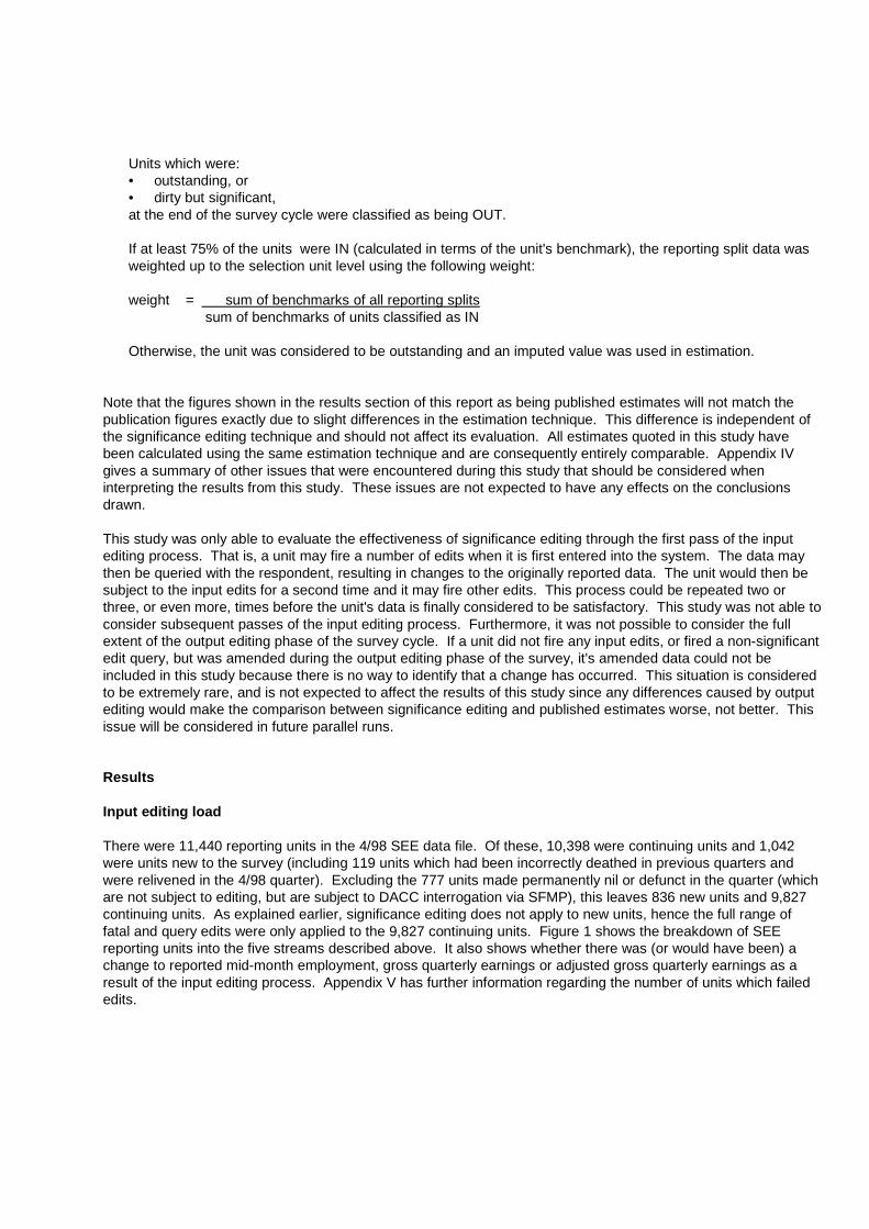
Note that the figures shown in the results section of this report as being published estimates will not match the publication figures exactly due to slight differences in the estimation technique. This difference is independent of the significance editing technique and should not affect its evaluation. All estimates quoted in this study have been calculated using the same estimation technique and are consequently entirely comparable. Appendix IV gives a summary of other issues that were encountered during this study that should be considered when interpreting the results from this study. These issues are not expected to have any effects on the conclusions drawn. This study was only able to evaluate the effectiveness of significance editing through the first pass of the input editing process. That is, a unit may fire a number of edits when it is first entered into the system. The data may then be queried with the respondent, resulting in changes to the originally reported data. The unit would then be subject to the input edits for a second time and it may fire other edits. This process could be repeated two or three, or even more, times before the unit's data is finally considered to be satisfactory. This study was not able to consider subsequent passes of the input editing process. Furthermore, it was not possible to consider the full extent of the output editing phase of the survey cycle. If a unit did not fire any input edits, or fired a non-significant edit query, but was amended during the output editing phase of the survey, it's amended data could not be included in this study because there is no way to identify that a change has occurred. This situation is considered to be extremely rare, and is not expected to affect the results of this study since any differences caused by output editing would make the comparison between significance editing and published estimates worse, not better. This issue will be considered in future parallel runs. Results Input editing load There were 11,440 reporting units in the 4/98 SEE data file. Of these, 10,398 were continuing units and 1,042 were units new to the survey (including 119 units which had been incorrectly deathed in previous quarters and were relivened in the 4/98 quarter). Excluding the 777 units made permanently nil or defunct in the quarter (which are not subject to editing, but are subject to DACC interrogation via SFMP), this leaves 836 new units and 9,827 continuing units. As explained earlier, significance editing does not apply to new units, hence the full range of fatal and query edits were only applied to the 9,827 continuing units. Figure 1 shows the breakdown of SEE reporting units into the five streams described above. It also shows whether there was (or would have been) a change to reported mid-month employment, gross quarterly earnings or adjusted gross quarterly earnings as a result of the input editing process. Appendix V has further information regarding the number of units which failed edits.

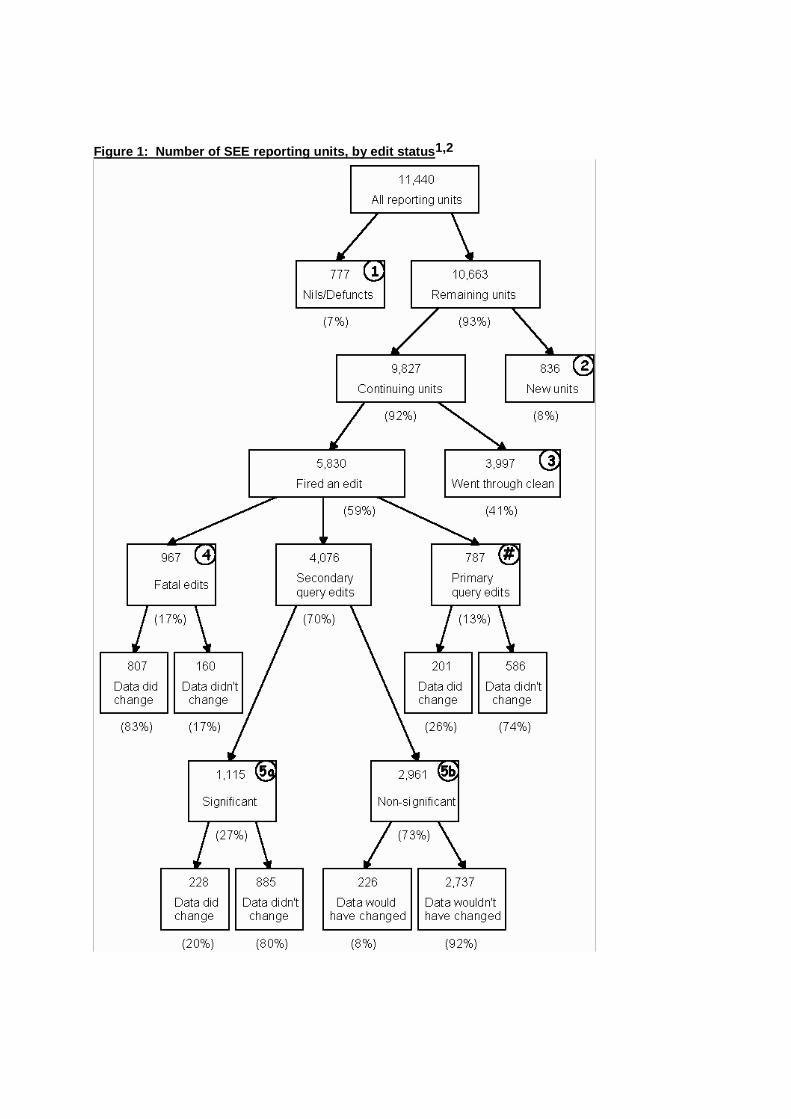
Figure 1: Number of SEE reporting units, by edit status1,2

1 Numbers in circles equate to the stream number. 2 To determine whether there was a change in the data, a comparison was made between the originally

reported and final edited data for the employment, gross quarterly earnings and adjusted gross quarterly earnings variables. As the full range of edits will encompass other survey variables, additional changes to the data may have occurred that are not evident in this figure.

# Primary query edits are units which failed a query edit that was considered to be inappropriate to be included in the significance editing process (Edit_31, Edit_65, Edit_68 and Edit_81 - see Appendix IV for further details). Such units are treated the same way as fatal units (in that their data is edited regardless of their significance) but conceptually, they are different. Significance editing only applies to units which fail secondary query edits.

It can be seen that almost 60% of continuing units fired at least one edit, half of which fired a non-significant edit query. This implies that the amount of input editing currently being performed in the survey is excessive, and that there is a potential for large savings during this phase of the survey. It is interesting to note that of the units which fired non-significant edit queries, only 8% would have had their data changed had they been edited. This emphasises the extent of input editing that can legitimately be avoided without significantly affecting the survey estimates. A higher proportion of units which failed significant edits (20%) and fatal edits (83%) had their data changed during the editing process. Given that the difference between originally reported data and edited data for these two streams of units is expected to be significant, it is appropriate that a larger proportion of the data is affected by the input editing process. (Note that, logically, units which fired fatal edits should all result in a change to their data. Since this figure only shows changes in the three major survey variables, the remaining 17% would presumably have resulted in changes to other survey variables). An estimate of the savings to be made can be calculated by considering all survey units, not just the continuing units, which have fired an edit. Of the 836 units new to the survey, it is estimated that approximately 75% (627) would have fired an edit (unfortunately, exact figures for new units are not available). This gives a total of 6,457 units which are expected to have fired an edit in the 4/98 quarter. If 2,961 of those units were not edited (because their query was considered to be non-significant), then this represents a resource saving of 46%. Given that approximately 20 full-time staff work on SEE for two months in the quarter, and 6 full-time staff work for the remaining month, and given that approximately a third of the staff time is spent on input editing, a 46% overall reduction in input editing equates to a saving of between 2 and 3 staff per quarter. Hence, by not editing units that have fired an edit query that is considered to be non-significant, an estimated 2 to 3 staff years could be saved (note that this figure may be slightly inflated as only the first pass of the input editing process could be considered). A more efficient placement for these staff could be in exploring aggregate level movements in the data so that reasons for movements in the final estimates can be better understood. Note that the expected resource savings of 2 to 3 staff years should be interpreted with caution. These figures are approximations only and do not take into account variables such as the complexity of edits. That is, queries that are easy to resolve will more than likely be classified as non-significant, thus leaving the more difficult (and time consuming) queries to resolve. Implementation of significance editing will also have the advantage of improving the alignment of recieval and clean rates for the survey. Since a large number of units which previously would have been edited can, effectively, be considered clean under significance editing, the preliminary estimates calculated for the National Accounts Branch will be based on a higher clean rate. Similarly, there should be a slight reduction in the amount of imputation that is needed at the preliminary estimation stage for units with reporting splits because previously dirty splits may not be significant under significance editing.

Effects on Survey Estimates Tables 1 and 2 show estimates of mid-month employment, by state and by industry, calculated using data from the significance editing study compared with published data. It can be seen that the significance editing estimates are only 0.1% lower than the published figures at the Australian level, which is less than one-tenth of the estimate's RSE% (1.1%). Even at the state and industry levels, the largest difference in estimates is only -0.2% and -0.6% respectively, which is reasonable, given the larger RSE%s at these levels. The tables also show that the accuracy of the estimates have not been affected by implementing significance editing. Table 1: Difference between published and significance editing estimates, mid-month employment by state, ('000)

Estimate RSE% Difference State

Published

Signif- icance

Editing

Published

Signif- icance Editing

Estimate

RSE% New South Wales 2,493.9 2,489.3 2.2 2.2 -0.2% 0.0 Victoria 1,785.6 1,783.8 2.3 2.3 -0.1% 0.0 Queensland 1,279.3 1,277.2 2.5 2.5 -0.2% 0.0 South Australia 528.3 528.4 2.9 2.9 0.0% 0.0 Western Australia 707.5 706.3 3.3 3.3 -0.2% 0.0 Tasmania 156.8 156.8 3.4 3.4 0.0% 0.0 Northern Territory 71.9 71.9 3.8 3.8 0.0% 0.0 Australian Capital Territory 142.1 142.0 3.3 3.3 -0.1% 0.0 Australia 7,165.4 7,155.6 1.1 1.1 -0.1% 0.0

Table 2: Difference between published and significance editing estimates, mid-month employment by industry division, ('000)

Estimate RSE% Difference Industry

Pub-

lished

Signif- icance

Editing

Pub-

lished

Signif- icance Editing

Estimate

RSE% A: Agriculture, Forestry and Fishing 5.8 5.8 3.8 3.8 0.0% 0.0 B: Mining 71.4 71.4 3.3 3.3 0.0% 0.0 C: Manufacturing 912.8 913.5 1.7 1.7 0.1% 0.0 D: Electricity, Gas and Water Supply 52.1 52.3 0.6 0.6 0.4% 0.0 E: Construction 365.5 364.3 6.5 6.5 -0.3% 0.0 F: Wholesale Trade 508.9 505.9 6.6 6.6 -0.6% 0.0 G: Retail Trade 1,056.2 1,052.5 3.6 3.6 -0.4% 0.0 H: Accommodation, Cafes and Restaurants 399.6 399.2 5.4 5.4 -0.1% 0.0 I: Transport and Storage 303.5 303.4 4.3 4.3 0.0% 0.0 J: Communication Services 122.5 122.5 4.6 4.6 0.0% 0.0 K: Finance and Insurance 295.7 296.1 4.9 4.9 0.1% 0.0 L: Property and Business Services 854.5 851.8 4.6 4.6 -0.3% 0.0 M: Government Administration and Defence 342.1 342.2 1.0 1.0 0.0% 0.0 N: Education 621.4 621.4 1.4 1.4 0.0% 0.0 O: Health and Community Services 794.2 794.2 2.1 2.1 0.0% 0.0 P: Cultural and Recreational Services 186.1 186.1 8.6 8.6 0.0% 0.0 Q: Personal and Other Services 273.0 272.8 4.0 4.0 -0.1% 0.0 Total All Industries 7,165.4 7,155.6 1.1 1.1 -0.1% 0.0

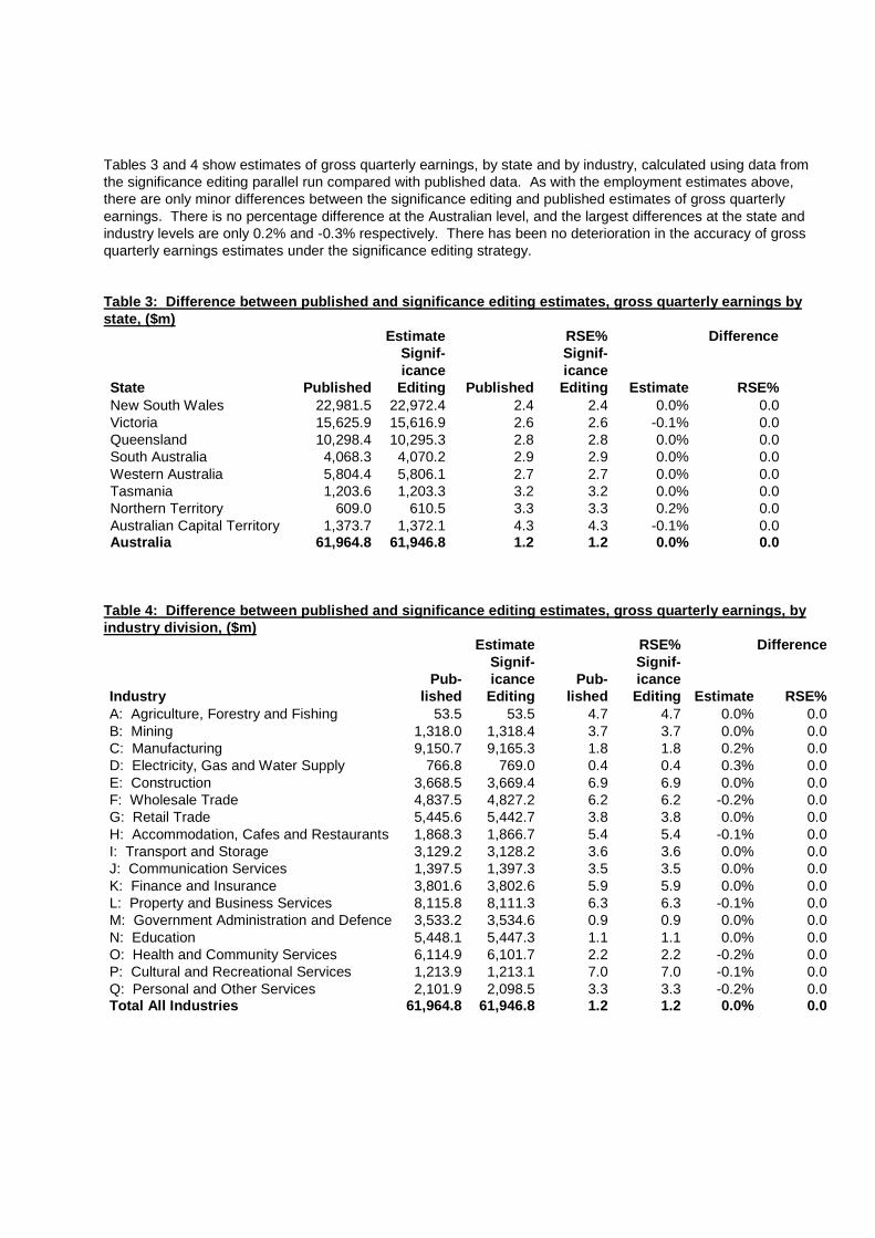
Tables 3 and 4 show estimates of gross quarterly earnings, by state and by industry, calculated using data from the significance editing parallel run compared with published data. As with the employment estimates above, there are only minor differences between the significance editing and published estimates of gross quarterly earnings. There is no percentage difference at the Australian level, and the largest differences at the state and industry levels are only 0.2% and -0.3% respectively. There has been no deterioration in the accuracy of gross quarterly earnings estimates under the significance editing strategy. Table 3: Difference between published and significance editing estimates, gross quarterly earnings by state, ($m)

Estimate RSE% Difference State

Published

Signif- icance

Editing

Published

Signif- icance Editing

Estimate

RSE% New South Wales 22,981.5 22,972.4 2.4 2.4 0.0% 0.0 Victoria 15,625.9 15,616.9 2.6 2.6 -0.1% 0.0 Queensland 10,298.4 10,295.3 2.8 2.8 0.0% 0.0 South Australia 4,068.3 4,070.2 2.9 2.9 0.0% 0.0 Western Australia 5,804.4 5,806.1 2.7 2.7 0.0% 0.0 Tasmania 1,203.6 1,203.3 3.2 3.2 0.0% 0.0 Northern Territory 609.0 610.5 3.3 3.3 0.2% 0.0 Australian Capital Territory 1,373.7 1,372.1 4.3 4.3 -0.1% 0.0 Australia 61,964.8 61,946.8 1.2 1.2 0.0% 0.0

Table 4: Difference between published and significance editing estimates, gross quarterly earnings, by industry division, ($m)

Estimate RSE% Difference Industry

Pub-

lished

Signif- icance

Editing

Pub-

lished

Signif- icance Editing

Estimate

RSE% A: Agriculture, Forestry and Fishing 53.5 53.5 4.7 4.7 0.0% 0.0 B: Mining 1,318.0 1,318.4 3.7 3.7 0.0% 0.0 C: Manufacturing 9,150.7 9,165.3 1.8 1.8 0.2% 0.0 D: Electricity, Gas and Water Supply 766.8 769.0 0.4 0.4 0.3% 0.0 E: Construction 3,668.5 3,669.4 6.9 6.9 0.0% 0.0 F: Wholesale Trade 4,837.5 4,827.2 6.2 6.2 -0.2% 0.0 G: Retail Trade 5,445.6 5,442.7 3.8 3.8 0.0% 0.0 H: Accommodation, Cafes and Restaurants 1,868.3 1,866.7 5.4 5.4 -0.1% 0.0 I: Transport and Storage 3,129.2 3,128.2 3.6 3.6 0.0% 0.0 J: Communication Services 1,397.5 1,397.3 3.5 3.5 0.0% 0.0 K: Finance and Insurance 3,801.6 3,802.6 5.9 5.9 0.0% 0.0 L: Property and Business Services 8,115.8 8,111.3 6.3 6.3 -0.1% 0.0 M: Government Administration and Defence 3,533.2 3,534.6 0.9 0.9 0.0% 0.0 N: Education 5,448.1 5,447.3 1.1 1.1 0.0% 0.0 O: Health and Community Services 6,114.9 6,101.7 2.2 2.2 -0.2% 0.0 P: Cultural and Recreational Services 1,213.9 1,213.1 7.0 7.0 -0.1% 0.0 Q: Personal and Other Services 2,101.9 2,098.5 3.3 3.3 -0.2% 0.0 Total All Industries 61,964.8 61,946.8 1.2 1.2 0.0% 0.0

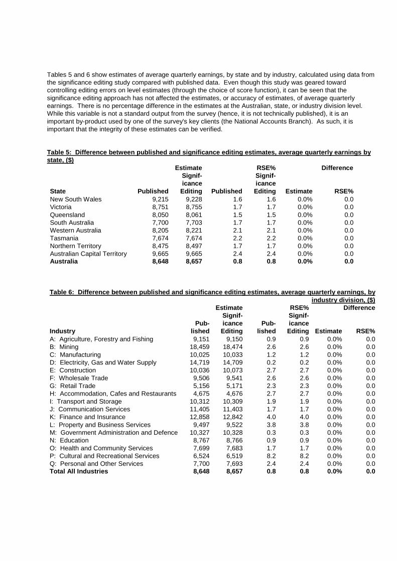
Tables 5 and 6 show estimates of average quarterly earnings, by state and by industry, calculated using data from the significance editing study compared with published data. Even though this study was geared toward controlling editing errors on level estimates (through the choice of score function), it can be seen that the significance editing approach has not affected the estimates, or accuracy of estimates, of average quarterly earnings. There is no percentage difference in the estimates at the Australian, state, or industry division level. While this variable is not a standard output from the survey (hence, it is not technically published), it is an important by-product used by one of the survey's key clients (the National Accounts Branch). As such, it is important that the integrity of these estimates can be verified. Table 5: Difference between published and significance editing estimates, average quarterly earnings by state, ($)

Estimate RSE% Difference State

Published

Signif- icance

Editing

Published

Signif- icance Editing

Estimate

RSE% New South Wales 9,215 9,228 1.6 1.6 0.0% 0.0 Victoria 8,751 8,755 1.7 1.7 0.0% 0.0 Queensland 8,050 8,061 1.5 1.5 0.0% 0.0 South Australia 7,700 7,703 1.7 1.7 0.0% 0.0 Western Australia 8,205 8,221 2.1 2.1 0.0% 0.0 Tasmania 7,674 7,674 2.2 2.2 0.0% 0.0 Northern Territory 8,475 8,497 1.7 1.7 0.0% 0.0 Australian Capital Territory 9,665 9,665 2.4 2.4 0.0% 0.0 Australia 8,648 8,657 0.8 0.8 0.0% 0.0

Table 6: Difference between published and significance editing estimates, average quarterly earnings, by

industry division, ($) Estimate RSE% Difference

Industry

Pub-

lished

Signif- icance

Editing

Pub-

lished

Signif- icance Editing

Estimate

RSE% A: Agriculture, Forestry and Fishing 9,151 9,150 0.9 0.9 0.0% 0.0 B: Mining 18,459 18,474 2.6 2.6 0.0% 0.0 C: Manufacturing 10,025 10,033 1.2 1.2 0.0% 0.0 D: Electricity, Gas and Water Supply 14,719 14,709 0.2 0.2 0.0% 0.0 E: Construction 10,036 10,073 2.7 2.7 0.0% 0.0 F: Wholesale Trade 9,506 9,541 2.6 2.6 0.0% 0.0 G: Retail Trade 5,156 5,171 2.3 2.3 0.0% 0.0 H: Accommodation, Cafes and Restaurants 4,675 4,676 2.7 2.7 0.0% 0.0 I: Transport and Storage 10,312 10,309 1.9 1.9 0.0% 0.0 J: Communication Services 11,405 11,403 1.7 1.7 0.0% 0.0 K: Finance and Insurance 12,858 12,842 4.0 4.0 0.0% 0.0 L: Property and Business Services 9,497 9,522 3.8 3.8 0.0% 0.0 M: Government Administration and Defence 10,327 10,328 0.3 0.3 0.0% 0.0 N: Education 8,767 8,766 0.9 0.9 0.0% 0.0 O: Health and Community Services 7,699 7,683 1.7 1.7 0.0% 0.0 P: Cultural and Recreational Services 6,524 6,519 8.2 8.2 0.0% 0.0 Q: Personal and Other Services 7,700 7,693 2.4 2.4 0.0% 0.0 Total All Industries 8,648 8,657 0.8 0.8 0.0% 0.0

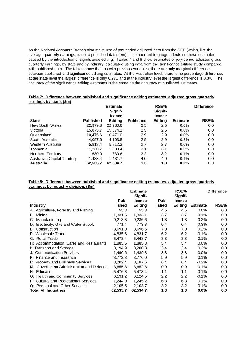
As the National Accounts Branch also make use of pay-period adjusted data from the SEE (which, like the average quarterly earnings, is not a published data item), it is important to gauge effects on these estimates caused by the introduction of significance editing. Tables 7 and 8 show estimates of pay-period adjusted gross quarterly earnings, by state and by industry, calculated using data from the significance editing study compared with published data. The tables show that, as with previous variables, there are only marginal differences between published and significance editing estimates. At the Australian level, there is no percentage difference, at the state level the largest difference is only 0.2%, and at the industry level the largest difference is 0.3%. The accuracy of the significance editing estimates is the same as the accuracy of published estimates. Table 7: Difference between published and significance editing estimates, adjusted gross quarterly earnings by state, ($m)

Estimate RSE% Difference State

Published

Signif- icance

Editing

Published

Signif- icance Editing

Estimate

RSE% New South Wales 22,979.3 22,980.6 2.5 2.5 0.0% 0.0 Victoria 15,875.7 15,874.2 2.5 2.5 0.0% 0.0 Queensland 10,475.6 10,471.0 2.9 2.9 0.0% 0.0 South Australia 4,097.6 4,103.8 2.9 2.9 0.2% 0.0 Western Australia 5,813.4 5,812.3 2.7 2.7 0.0% 0.0 Tasmania 1,230.7 1,230.4 3.1 3.1 0.0% 0.0 Northern Territory 630.0 630.6 3.2 3.2 0.1% 0.0 Australian Capital Territory 1,433.4 1,431.7 4.0 4.0 0.1% 0.0 Australia 62,535.7 62,534.7 1.3 1.3 0.0% 0.0

Table 8: Difference between published and significance editing estimates, adjusted gross quarterly earnings, by industry division, ($m)

Estimate RSE% Difference Industry

Pub-

lished

Signif- icance

Editing

Pub-

lished

Signif- icance Editing

Estimate

RSE% A: Agriculture, Forestry and Fishing 55.3 55.3 4.5 4.5 0.0% 0.0 B: Mining 1,331.6 1,333.1 3.7 3.7 0.1% 0.0 C: Manufacturing 9,218.8 9,236.6 1.8 1.8 0.2% 0.0 D: Electricity, Gas and Water Supply 771.4 773.8 0.4 0.4 0.3% 0.0 E: Construction 3,691.0 3,696.5 7.0 7.0 0.2% 0.0 F: Wholesale Trade 4,835.6 4,831.7 6.2 6.2 -0.1% 0.0 G: Retail Trade 5,473.4 5,468.7 3.8 3.8 -0.1% 0.0 H: Accommodation, Cafes and Restaurants 1,885.5 1,885.3 5.4 5.4 0.0% 0.0 I: Transport and Storage 3,194.9 3,200.8 3.4 3.4 0.2% 0.0 J: Communication Services 1,490.6 1,489.8 3.3 3.3 0.0% 0.0 K: Finance and Insurance 3,772.3 3,776.0 5.9 5.9 0.1% 0.0 L: Property and Business Services 8,202.4 8,187.6 6.4 6.4 -0.2% 0.0 M: Government Administration and Defence 3,655.3 3,652.8 0.9 0.9 -0.1% 0.0 N: Education 5,476.8 5,473.4 1.1 1.1 -0.1% 0.0 O: Health and Community Services 6,131.2 6,124.5 2.2 2.2 -0.1% 0.0 P: Cultural and Recreational Services 1,244.0 1,245.2 6.8 6.8 0.1% 0.0 Q: Personal and Other Services 2,105.5 2,103.7 3.2 3.2 -0.1% 0.0 Total All Industries 62,535.7 62,534.7 1.3 1.3 0.0% 0.0

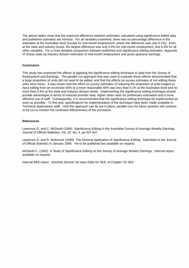
The above tables show that the expected difference between estimates calculated using significance edited data and published estimates are minimal. For all variables examined, there was no percentage difference in the estimates at the Australian level (except for mid-month employment, where the difference was only 0.1%). Even at the state and industry levels, the largest difference was only 0.6% for mid-month employment, and 0.3% for all other variables. For a more detailed comparison between published and significance editing estimates, Appendix VI shows state by industry division estimates of mid-month employment and gross quarterly earnings. Conclusion This study has examined the effects of applying the significance editing technique to data from the Survey of Employment and Earnings. The parallel run approach that was used to evaluate these effects demonstrated that a large proportion of units did not need to be edited, and that the effects on survey estimates of not editing these units were minor. It was shown that the effect on survey estimates of reducing the proportion of units subject to input editing from an excessive 65% to a more reasonable 40% was less than 0.1% at the Australian level and no more than 0.6% at the state and industry division levels. Implementing the significance editing technique should provide advantages in terms of reduced provider load, higher clean rates for preliminary estimation and a more effective use of staff. Consequently, it is recommended that the significance editing technique be implemented as soon as possible. To this end, specifications for implementation of the technique have been made available to Technical Applications staff. Until this approach can be put in place, parallel runs for future quarters will continue to be run to monitor the continued effectiveness of the procedure. References Lawrence D. and C. McDavitt (1994) Significance Editing in the Australian Survey of Average Weekly Earnings. Journal of Official Statistics, Vol. 10. No. 4, pp 437-447. Lawrence D. and R. McKenzie (1999) The General Application of Significance Editing. Submitted to the Journal of Official Statistics in January 1999. Yet to be published but available on request. McDavitt C. (1992) A Study of Significance Editing on the Survey of Average Weekly Earnings. Internal report, available on request. Internal ABS report: (doclink) Section '02 Input Edits for SEE' of Chapter '02 SEE '

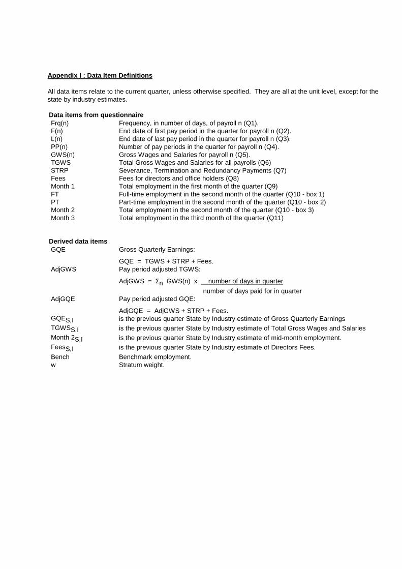
Appendix I : Data Item Definitions All data items relate to the current quarter, unless otherwise specified. They are all at the unit level, except for the state by industry estimates. Data items from questionnaire Frq(n) Frequency, in number of days, of payroll n (Q1). F(n) End date of first pay period in the quarter for payroll n (Q2). L(n) End date of last pay period in the quarter for payroll n (Q3). PP(n) Number of pay periods in the quarter for payroll n (Q4). GWS(n) Gross Wages and Salaries for payroll n (Q5). TGWS Total Gross Wages and Salaries for all payrolls (Q6) STRP Severance, Termination and Redundancy Payments (Q7) Fees Fees for directors and office holders (Q8) Month 1 Total employment in the first month of the quarter (Q9) FT Full-time employment in the second month of the quarter (Q10 - box 1) PT Part-time employment in the second month of the quarter (Q10 - box 2) Month 2 Total employment in the second month of the quarter (Q10 - box 3) Month 3 Total employment in the third month of the quarter (Q11)

Derived data items GQE Gross Quarterly Earnings:

GQE = TGWS + STRP + Fees. AdjGWS Pay period adjusted TGWS:

AdjGWS = Σn GWS(n) x number of days in quarter

number of days paid for in quarter AdjGQE Pay period adjusted GQE:

AdjGQE = AdjGWS + STRP + Fees. GQES,I is the previous quarter State by Industry estimate of Gross Quarterly Earnings TGWSS,I is the previous quarter State by Industry estimate of Total Gross Wages and Salaries Month 2S,I is the previous quarter State by Industry estimate of mid-month employment. FeesS,I is the previous quarter State by Industry estimate of Directors Fees.

Bench Benchmark employment. w Stratum weight.

Appendix II - Edit Specifications The attached Wordpro document contains the list of edits used in the SEE with their corresponding score functions. This document should form the basis of the edit specifications. It is available in hardcopy (on request) for those without Wordpro access.

Sigedapp.lwp Alternatively, it can be viewed using Word:

Sigedapp.doc

Appendix III - State by Industry Cut-off Scores There were nine state by industry cells where the cut-off score could not be determined because all units in the cell were enumerated. As a result, there was no sampling variability in the cell and the cut-off score was set to zero. In such cases, it is important to approximate a cut-off score, otherwise all units in the cell will be subject to input editing, regardless of whether the edit query is significant or not, which results in an inefficient use of resources. Consequently, these nine cut-off scores were calculated clerically, using information from other states and industries. The technique used to perform this clerical imputation was based on the knowledge that cut-off scores are dependent on the state by industry standard error (and consequently, the state by industry estimate) of gross quarterly earnings. The missing cut-off scores should hence be calculated by taking into account the relative size of the estimate in the cell. The technique used to calculate the missing cut-off scores involved calculating the ratio between the cut-off score and the estimate for every state by industry cell with a valid cut-off score. These ratios were then averaged across all states with valid cut-off scores within a particular industry, and were then multiplied by the estimate in the state with an invalid cut-off score. For example, consider the Agriculture, Forestry and Fishing industry division. All states except for New South Wales, Victoria and Queensland in this industry had missing cut-off scores. For New South Wales, the estimate of gross quarterly earnings was $19.7m (median smoothed over December quarter 1997 to September quarter 1998), the cut-off score was $45,096 and the ratio of these two values was 0.0023. For Victoria, the ratio was 0.2705 and for Queensland, it was 0.0254, resulting in an average ratio of 0.0994. Multiplying the average ratio by the South Australian estimate ($2.1m) gives an approximate cut-off score for South Australia of $208,740. This process was used for the remaining invalid cut-off scores. Table A1 shows the full set of cut-off scores, including the clerically imputed ones. This data is also available electronically upon request (in spreadsheet or SASDB format). It is recommended that the cut-off scores be reviewed from time to time to determine whether the levels set in this study remain appropriate. If a sample redesign is performed for the survey, this review will be mandatory.

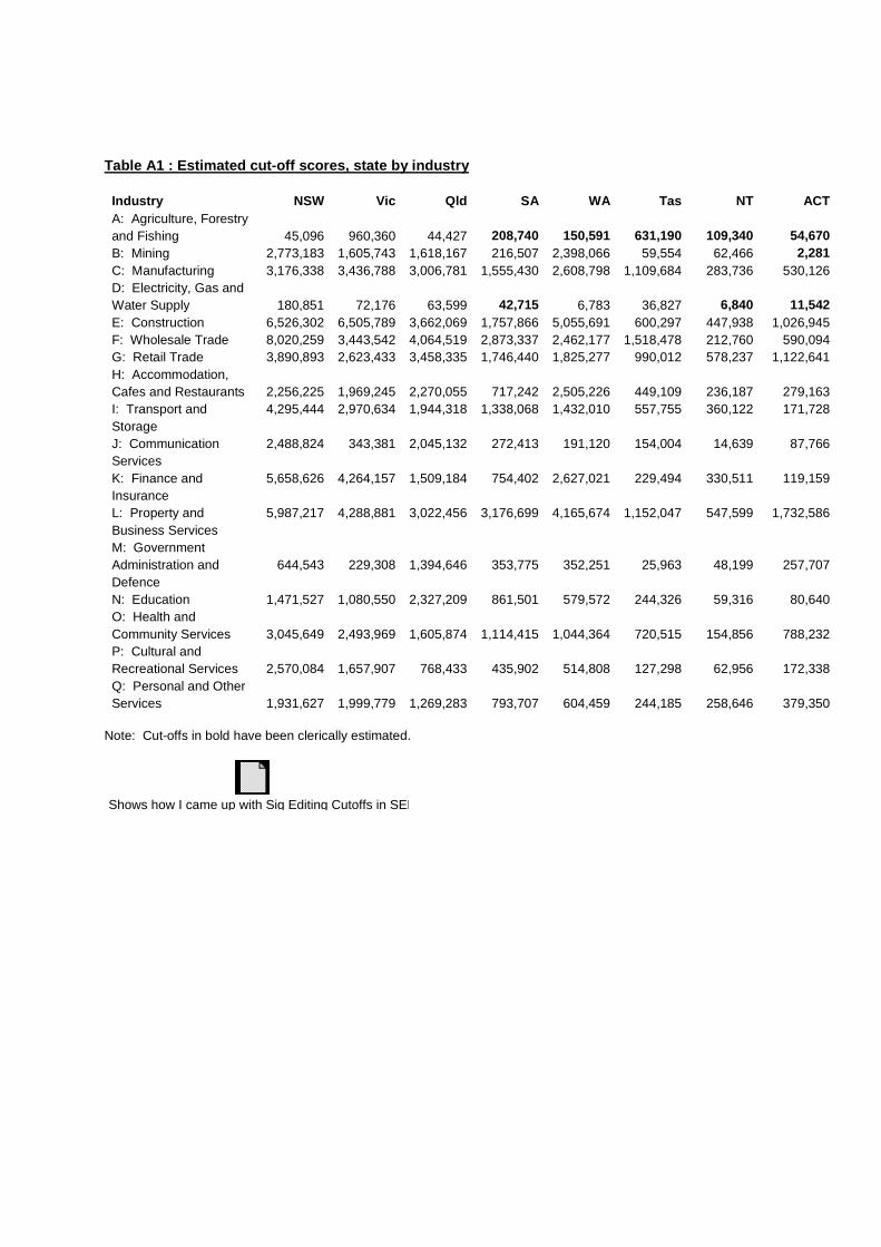
Table A1 : Estimated cut-off scores, state by industry

Industry NSW Vic Qld SA WA Tas NT ACT A: Agriculture, Forestry and Fishing

45,096

960,360

44,427

208,740

150,591

631,190

109,340

54,670

B: Mining 2,773,183 1,605,743 1,618,167 216,507 2,398,066 59,554 62,466 2,281 C: Manufacturing 3,176,338 3,436,788 3,006,781 1,555,430 2,608,798 1,109,684 283,736 530,126 D: Electricity, Gas and Water Supply

180,851

72,176

63,599

42,715

6,783

36,827

6,840

11,542

E: Construction 6,526,302 6,505,789 3,662,069 1,757,866 5,055,691 600,297 447,938 1,026,945 F: Wholesale Trade 8,020,259 3,443,542 4,064,519 2,873,337 2,462,177 1,518,478 212,760 590,094 G: Retail Trade 3,890,893 2,623,433 3,458,335 1,746,440 1,825,277 990,012 578,237 1,122,641 H: Accommodation, Cafes and Restaurants

2,256,225

1,969,245

2,270,055

717,242

2,505,226

449,109

236,187

279,163

I: Transport and Storage

4,295,444 2,970,634 1,944,318 1,338,068 1,432,010 557,755 360,122 171,728

J: Communication Services

2,488,824 343,381 2,045,132 272,413 191,120 154,004 14,639 87,766

K: Finance and Insurance

5,658,626 4,264,157 1,509,184 754,402 2,627,021 229,494 330,511 119,159

L: Property and Business Services

5,987,217 4,288,881 3,022,456 3,176,699 4,165,674 1,152,047 547,599 1,732,586

M: Government Administration and Defence

644,543

229,308

1,394,646

353,775

352,251

25,963

48,199

257,707

N: Education 1,471,527 1,080,550 2,327,209 861,501 579,572 244,326 59,316 80,640 O: Health and Community Services

3,045,649

2,493,969

1,605,874

1,114,415

1,044,364

720,515

154,856

788,232

P: Cultural and Recreational Services

2,570,084

1,657,907

768,433

435,902

514,808

127,298

62,956

172,338

Q: Personal and Other Services

1,931,627

1,999,779

1,269,283

793,707

604,459

244,185

258,646

379,350

Note: Cut-offs in bold have been clerically estimated.

Shows how I came up with Sig Editing Cutoffs in SEE

Appendix IV : Issues to consider There are a number of issues which were encountered during the testing phase of the significance editing parallel run which should be taken into consideration when interpreting the results. These are described below.

There were approximately 1,500 businesses on the frame which had been incorrectly deathed in previous quarters. These were relivened in the 4/98 quarter and should have been recorded on the original data file as being new to the survey. As this did not happen, they were explicitly excluded from the significance editing process and treated as though they were new to the survey. This affected 119 units. A number of units were discovered which became permanently nil or defunct partway through the quarter. These units contributed zero to the estimates, even though they should have contributed for the part of the quarter when they were active. This discrepancy is due to a system problem. The LSC Output group are aware of the situation and will ensure that the system is fixed in time for next quarter's estimation. There were a handful of cases where the first pay date recorded was later than the last pay date for a given payroll. It is not possible to guarantee that this sort of error will be identified by the edits. It is recommended that the input processing system be modified so that this circumstance is not allowed. Query edits 36 to 39 were not incorporated into this study as they are not expected to affect the data items. These edits are only double checks to ensure the validity of the CNDU flag (Ceased reporting split, permanently Nil unit, Defunct unit, or Untraceable unit). Significance edit numbers 16 and 17 were not tested as they were added in at the end of this study to be consistent with Edit_47 and Edit_56 respectively. Scaled local score functions were specified for significance edit numbers 11 and 12, but they were not tested in this study as it was too difficult to derive the program code that matches payrolls across time.

During the testing process, any scaled local scores that were zero were investigated to ensure the validity of the score functions. Some examples are listed below.

There were five units where the scaled local score was zero for significance edit number 3. This was due to the fact that the previous quarter employment was also zero. In such cases, it is important that the unit is edited, hence the score was reset to 9,999,999, to ensure that it will be higher than all the cut-offs and thus be classed as significant. There were twenty-five units where the scaled local score was zero for significance edit number 4. This was due to the fact that the average employment (calculated over the non-zero months) was zero. Under normal circumstances such units would be identified in significance edit number 2 or 3. However, since these units did not report any employment or gross wages and salaries, they were not identified in these edits. As the units did report directors fees and/or severance, termination and redundancy pay, this is a valid situation and there is no need to edit such units. There were two units where the scaled local score was zero for significance edit number 7. This was due to the fact that the payroll GWS was zero, and thus the modified GWS was equivalent to the original GWS. Such units will be identified in fatal Edit_03.

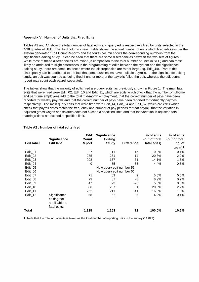
Appendix V : Number of Units that Fired Edits Tables A3 and A4 show the total number of fatal edits and query edits respectively fired by units selected in the 4/98 quarter of SEE. The third column in each table shows the actual number of units which fired edits (as per the system generated "Edit Count Report") and the fourth column shows the corresponding numbers from the significance editing study. It can be seen that there are some discrepancies between the two sets of figures. While most of these discrepancies are minor (in comparison to the total number of units in SEE) and can most likely be attributed to slight differences in the programming of edits between the system and the significance editing study, there are some instances where the discrepancies are rather large (eg. Edit_44). Part of this discrepancy can be attributed to the fact that some businesses have multiple payrolls. In the significance editing study, an edit was counted as being fired if one or more of the payrolls failed the edit, whereas the edit count report may count each payroll separately. The tables show that the majority of edits fired are query edits, as previously shown in Figure 1. The main fatal edits that were fired were Edit_02, Edit_10 and Edit_11, which are edits which check that the number of full-time and part-time employees add to the total mid-month employment, that the correct number of pays have been reported for weekly payrolls and that the correct number of pays have been reported for fortnightly payrolls, respectively. The main query edits that were fired were Edit_44, Edit_64 and Edit_67, which are edits which check that payroll dates match the frequency and number of pay periods for that payroll, that the variation in adjusted gross wages and salaries does not exceed a specified limit, and that the variation in adjusted total earnings does not exceed a specified limit. Table A2 : Number of fatal edits fired Edit label

Significance Edit label

Edit Count

Report

Significance Editing

Study

Difference

% of edits (out of total fatal edits)

% of edits (out of total

no. of units)1

Edit_01 27 11 16 0.9% 0.1% Edit_02 275 261 14 20.8% 2.2% Edit_03 208 177 31 14.1% 1.5% Edit_04 0 55 -55 4.4% 0.5% Edit_05 Now query edit number 55. Edit_06 Now query edit number 56. Edit_07 71 69 2 5.5% 0.6% Edit_08 79 87 -8 6.9% 0.7% Edit_09 47 73 -26 5.8% 0.6% Edit_10 308 257 51 20.5% 2.2% Edit_11 252 211 41 16.8% 1.8% Edit_12 Significance

editing not applicable to fatal edits.

58 52 6 4.2% 0.4%

Total 1,325 1,253 72 100.0% 10.6% 1 Note that the total no. of units is taken as the total number of reporting units in the survey (11,829).

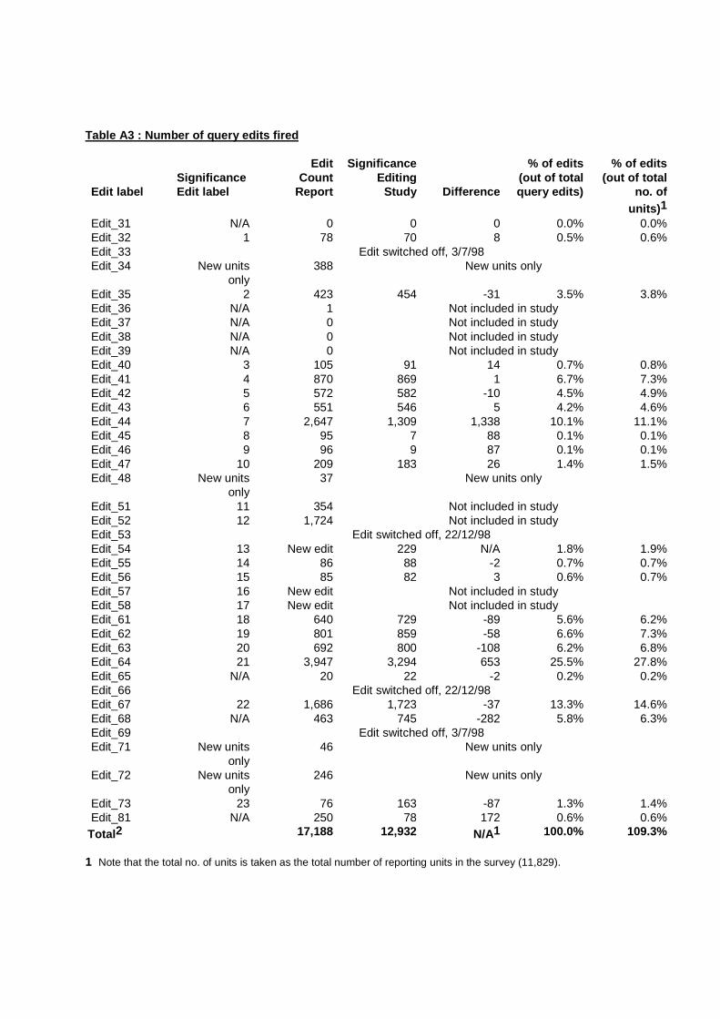
Table A3 : Number of query edits fired Edit label

Significance Edit label

Edit Count

Report

Significance Editing

Study

Difference

% of edits (out of total query edits)

% of edits (out of total

no. of units)1

Edit_31 N/A 0 0 0 0.0% 0.0% Edit_32 1 78 70 8 0.5% 0.6% Edit_33 Edit switched off, 3/7/98 Edit_34 New units

only 388 New units only

Edit_35 2 423 454 -31 3.5% 3.8% Edit_36 N/A 1 Not included in study Edit_37 N/A 0 Not included in study Edit_38 N/A 0 Not included in study Edit_39 N/A 0 Not included in study Edit_40 3 105 91 14 0.7% 0.8% Edit_41 4 870 869 1 6.7% 7.3% Edit_42 5 572 582 -10 4.5% 4.9% Edit_43 6 551 546 5 4.2% 4.6% Edit_44 7 2,647 1,309 1,338 10.1% 11.1% Edit_45 8 95 7 88 0.1% 0.1% Edit_46 9 96 9 87 0.1% 0.1% Edit_47 10 209 183 26 1.4% 1.5% Edit_48 New units

only 37 New units only

Edit_51 11 354 Not included in study Edit_52 12 1,724 Not included in study Edit_53 Edit switched off, 22/12/98 Edit_54 13 New edit 229 N/A 1.8% 1.9% Edit_55 14 86 88 -2 0.7% 0.7% Edit_56 15 85 82 3 0.6% 0.7% Edit_57 16 New edit Not included in study Edit_58 17 New edit Not included in study Edit_61 18 640 729 -89 5.6% 6.2% Edit_62 19 801 859 -58 6.6% 7.3% Edit_63 20 692 800 -108 6.2% 6.8% Edit_64 21 3,947 3,294 653 25.5% 27.8% Edit_65 N/A 20 22 -2 0.2% 0.2% Edit_66 Edit switched off, 22/12/98 Edit_67 22 1,686 1,723 -37 13.3% 14.6% Edit_68 N/A 463 745 -282 5.8% 6.3% Edit_69 Edit switched off, 3/7/98 Edit_71 New units

only 46 New units only

Edit_72 New units only

246 New units only

Edit_73 23 76 163 -87 1.3% 1.4% Edit_81 N/A 250 78 172 0.6% 0.6%

Total2 17,188 12,932 N/A1 100.0% 109.3% 1 Note that the total no. of units is taken as the total number of reporting units in the survey (11,829).

2 Note that the total for the edit count report column (17,188) is not comparable to the total from the significance editing study total (12,932) as i) the significance edit study did not consider those edits that were applicable to new units only, ii) there were a number of edits that were not included in the significance edit study, and iii) there were new edits introduced that would not appear in the edit count report.

Appendix VI : State by Industry estimates Internal ABS report: (doclink) (Database: "MD Proj Vol 2 - PSG Client WDB"; Subject: "Appendix VI : State by Industry estimates"; Author: Gabriela Lawrence; Date Created: 29/11/2000)