Simulation Based Comparison of FourSite-Response Estimation TechniquesFabien Coutel and Peter Mora

Q.U.A.K.E.SThe University of Queensland4072 Qld, BrisbaneAUSTRALIAE-mail: coutel@earthsciences.uq.edu.au, mora@earthsciences.uq.edu.auTelephone: +61 7 3365 4853, +61 7 3365 2128Facsimile: (07) 3365 7347Submitted to theBulletin of the Seismological Society of AmericaManuscript # : 97029

AbstractRecent earthquakes have triggered renewed interest to better understand earthquake siteresponse. Most of the studies comparing various techniques for estimating site response werebased on real data (from earthquakes, nuclear blasts and seismic noise). A theoretical approach,using synthetic data generated with the pseudospectral method is used to compare four site-response estimation techniques. The limits of applicability of each method were determined bymodeling microtremors and incoming SV-waves (with di�erent incidence angles) and analysingthe site ampli�cations. The �rst two techniques investigated consist of dividing the spectrumof the horizontal motion at a site by that of a reference site using either incident S-wavesor microtremors. The latter was unable to reveal either the resonant frequencies or peakamplitudes in any cases. The two other techniques are based on the horizontal-to-verticalspectral ratio using S-waves or microtremors. These techniques were found to reveal at leastthe fundamental resonant frequency and amplitude (former method only) within 10% error, inthe case of simple geology ( at layers). However, the results show that these techniques areunable to take into account 2D e�ects such as focusing e�ects and basin-edge e�ects and yieldunreliable or incorrect results in such cases.

2

IntroductionThrough the study of numerous earthquakes, it has long been understood that consider-able modi�cation of the seismic signal may result from topographic and local geological e�ects.The severe consequences of these phenomena were recently experienced during the 1985 Mi-choacan Mexico earthquake (e.g., Singh et al., 1988) and the 1989 Loma Prieta earthquake (e.g.,Hough et al., 1990). These cases triggered renewed interest of researchers in understanding siteampli�cations to better assess seismic hazard.It is therefore necessary to develop methods for �rst identifying regions prone to siteampli�cations, and ultimately quantifying this phenomenon. In order to estimate site-response,one can use either an empirical approach (using seismic recordings) or a theoretical approach(using synthetics generated with modeling methods).Various site-response estimation techniques have been already studied through the com-parison of mainshocks, aftershocks or seismic noise recordings (e.g., Field and Jacob, 1993;Lermo and Ch�avez-Garc��a, 1994; Clitheroe and Taber, 1995; Lachet et al., 1996; Seekins et al.,1996). In this paper, we focus on those that predict site ampli�cation at particular sites. Thesetechniques can be separated into two categories : those that use at least two sites and thosethat use one site only. Borcherdt (1970) introduced the sediment-to-bedrock ratio (that is stillthe most common approach) which consists of dividing the spectrum of a site by that of anearby reference site (rock site) using earthquakes. This approach identi�es the fundamentalresonant frequency of a site in most cases (e.g., Jarpe et al., 1988; Darragh and Shakal, 1991;Margheriti et al., 1994) and is often considered to be the most reliable. However, the choice ofthe reference site remains critical: rock sites can have their own site response which can leadto an underestimation of the site response (e.g., Steidtl et al., 1996).Several studies (e.g., Ohta et al., 1978; Yamanaka et al., 1994) applied the approach ofBorcherdt, using ambient seismic noise instead of earthquakes. These studies found that theratios from long period seismic noise (microseisms) and strong motion records produced similarpredominant periods. Shorter period noise (microtremor) has also been used to �nd dominantperiods, but its use is questionable (e.g., Ohta et al., 1978; Bard, 1995).An alternative method, requiring only one recording station, consists of dividing thespectrum of the horizontal component by that of the vertical component. Nakamura (1989)�rst introduced the horizontal-to-vertical noise ratio, using microtremors to estimate site am-pli�cation. Although there is little theoretical justi�cation for Nakamura's technique, it hasbeen observed in numerical experiments (e.g., Lermo and Ch�avez-Garc��a, 1994; Lachet andBard, 1994) that if microtremors consist of Rayleigh waves propagating in a single layer over ahalf-space, Nakamura's ratio can reveal the fundamental resonant frequency. In addition, La-chet and Bard (1994) concluded that the amplitude of the horizontal-to-vertical noise ratio isquite sensitive to the source-receiver distance while being independent of the source excitationfunction. Other numerical experiments (e.g., Field and Jacob, 1993; Dravinski et al., 1996)demonstrated that Nakamura's technique predicts only the fundamental resonant frequency(to within approximately 10 percent) and found discrepancies with the predicted amplitude.Empirical studies (e.g., Lermo and Ch�avez-Garc��a, 1994; Clitheroe and Taber, 1995; Field andJacob, 1995; Lachet et al., 1996; Seekins et al., 1996) showed that although the fundamentalfrequency can be determined with a reasonable precision, higher modes cannot: Lermo andCh�avez-Garc��a (1994) suggested that this observation was due to the presence of Rayleighwaves in microtremors. Despite these observations, there remains little theoretical justi�ca-tion for using Nakamura's technique in complex geological models, with no current consensusamongst researchers regarding its limits of applicability.Lermo and Ch�avez-Garc��a (1993) applied Nakamura's technique to single earthquakes andconcluded that in the case of simple geology this approach was able to reliably estimate thefrequency and amplitude of the fundamental resonant mode. Thus, it provides an economic3

alternative (only one station needed) to Borcherdt's approach. Other studies showed that thehorizontal-to-vertical spectral ratio can provide partial information on the site response, suchas the fundamental resonant frequencies (e.g., Field, 1996; Lachet et al., 1996) and in somecases all the other resonant frequencies (Field and Jacob, 1995). Some studies have found thatthe horizontal-to-vertical spectral ratio predicts a correct ampli�cation level (e.g., Lermo andCh�avez-Garc��a, 1993), others do not (Field and Jacob, 1995).To investigate the di�erence between these methods and to seek out the applicability ofNakamura's technique for 2D models, we propose a more theoretical approach of simulating thesite ampli�cation by numerical modeling. Various modeling techniques (such as pseudospectral,�nite-element or boundary integral methods) are available and enable one to include complexstructures and rheologies. In addition, modeling studies supplement empirical studies by allow-ing one to explore the sensitivity of site response with respect to variations in incidence angle,azimuth and wave type. Although more realistic models are now feasible, very few attempts tocompare site-response techniques have employed them (Dravinski et al., 1996). However, forsimpler models, several studies have already provided limited information about the reliabilityof the H=V ratio using seismic noise and SV waves (e.g., Field and Jacob, 1993; Lermo andCh�avez-Garc��a, 1994; Lachet and Bard, 1994).Here, we make use of the pseudospectral modeling technique because of its capacity tomodel di�erent types of waves (e.g., Rayleigh waves and Love waves) at the free surface andin depth with a high accuracy, and its ease of implementation (e.g., Carcione and Wang, 1993;Komatitsch et al., 1996). Numerical experiments are performed by modeling earthquake wavesas incoming plane S-waves with di�erent incident angles and microtremors as random forces atthe free surface.Methods used to determine site ampli�cationsSince seismic recordings are in uenced by source, path and site e�ects, it is necessary toremove the �rst two e�ects in order to isolate the ampli�cations of seismic waves at a givensite. Several techniques have been proposed, in this paper we will focus on four previously citedapproaches.Sediment to bedrock spectral ratio (SBSR)The most common technique used for estimating site response is the standard spectralratio procedure �rst introduced by Borcherdt (1970). The spectrum of the site of interest isdivided by that of a nearby reference site (preferably situated on bedrock). The hypothesis inthis case is that the two sites have similar source and path e�ects and that the reference site,having a negligible site response, should have a at spectrum response. Hence, the resultingspectral ratio SR = HSHR ; (1)where HS and HR denote the horizontal frequency spectrum at the site of interest and referencesite respectively, should constitute a good estimate of site response.Sediment to bedrock noise ratio (SBNR)This technique is based on Borcherdt's proposal, the di�erence being that the backgroundseismic noise (preferably long period) is used. The sediment-to-bedrock noise ratio is thusderived by equation (1).Horizontal to vertical noise ratio (HVNR)4

An alternative method for removing source e�ects was proposed by Nakamura (1989).This technique, based on microtremors (short period seismic noise), gained the interest of manyresearchers because of its low cost, rapidity of �eld operations (recording of background noisewith only a few stations) and the simplicity of the analysis (it is not necessary to hand-pick timewindows). Nakamura claimed that over a large range of frequencies, the vertical componentof ambient noise is relatively unin uenced by a soft sediment layer overlying a half-space. Hethen proposed to compute the ratio SN = HSVS ; (2)where HS and VS respectively denote the horizontal and vertical frequency spectrum computedat a sediment site. Equation (2) relies on the hypothesisHBVB � 1 ; (3)where HB and VB respectively denote the horizontal and vertical frequency spectrum computedat the base of the sediment layer.Horizontal to vertical spectral ratio (HVSR)This technique is based on Nakamura's hypothesis (Eq. 3), the di�erence being thatsingle earthquakes are used instead of microtremors. The horizontal-to-vertical spectral ratiois derived by equation (2). Numerical modelingThe Pseudospectral methodThe pseudospectral modeling scheme used in this paper is the same as in Carcione (1994)and Komatitsch et al. (1996).The wave-equation is written in the velocity-stress formulation (Virieux, 1986) in carte-sian coordinates. It is solved �rst by computing the spatial derivatives in the curved gridsystem, and then the chain rule is applied to calculate the required cartesian spatial deriva-tives. Chebyshev di�erential operators are used to compute the derivatives in both vertical andhorizontal directions.The Chebyshev algorithm has been chosen because it is free of numerical dispersion up to� points per wavelength (Koslo� and Tal-Ezer, 1993), and because boundary conditions such asthe free surface condition can be implemented in a straightforward and e�cient way (Carcioneand Wang, 1993).Source implementationAs explained previously, the four techniques used in this study are applied to di�erentparts of the seismic signal. The sediment-to-bedrock and horizontal-to-vertical ratios are ap-plied to both S-waves and seismic noise records. Thus, it is necessary to implement numericallythese two di�erent types of source.Incoming plane wave. The main challenge in determining site ampli�cation characteristics isto remove both source and path e�ects. A simple solution is to use a source that is distantfrom the receivers. In this case, the waves are quasi-plane waves when they reach the regionof interest so the approximation of a plane wave is reasonable. Moreover, S-waves generallyproduce higher ampli�cations than P-waves because of a higher Poisson's ratio in the surface5

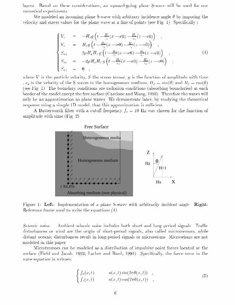
layers. Based on these considerations, an upward-going plane S-wave will be used for ournumerical experiments.We modeled an incoming plane S-wave with arbitrary incidence angle � by imposing thevelocity and stress values for the plane wave at a line of points (see Fig. 1). Speci�cally :8>>>>>>>><>>>>>>>>:Vx = �Hzg �t� Hxcs (x� x0)� Hzcs (z � z0)� ;Vz = Hxg �t� Hxcs (x� x0)� Hzcs (z � z0)� ;Sxx = 2�HxHz g �t� Hxcs (x� x0)� Hzcs (z � z0)� ;Szz = �2�HxHz g �t� Hxcs (x� x0)� Hzcs (z � z0)� ;Sxz = 0 ; (4)where V is the particle velocity, S the stress tensor, g is the function of amplitude with time, cs is the velocity of the S waves in the homogeneous medium, Hx = sin(�) and Hz = cos(�)(see Fig. 1). The boundary conditions are radiation conditions (absorbing boundaries) at eachborder of the model except the free surface (Carcione and Wang, 1993). Therefore the waves willonly be an approximation to plane waves. We demonstrate later, by studying the theoreticalresponse using a simple 1D model, that this approximation is su�cient.A Butterworth �lter with a cuto� frequency fc = 10 Hz was chosen for the function ofamplitude with time (Fig. 2).θ

Absorbing medium (non physical)

Free Surface

( X0,Z0)

Homogeneous medium

Heterogeneous media

X

Z

H=1

Hx

HzFigure 1: Left: Implementation of a plane S-wave with arbitrarily incident angle. Right:Reference frame used to write the equations (4).Seismic noise. Ambient seismic noise includes both short and long period signals. Tra�cdisturbances or wind are the origin of short-period signals, also called microtremors, whiledistant oceanic disturbances result in long-period signals or microseisms. Microseisms are notmodeled in this paper.Microtremors can be modeled as a distribution of impulsive point forces located at thesurface (Field and Jacob, 1993; Lachet and Bard, 1994). Speci�cally, the force term in thewave equation is written: ( fx(x; t) = a(x; t) sin(2��(x; t)) ;fz(x; t) = a(x; t) cos(2��(x; t)) ; (5)6

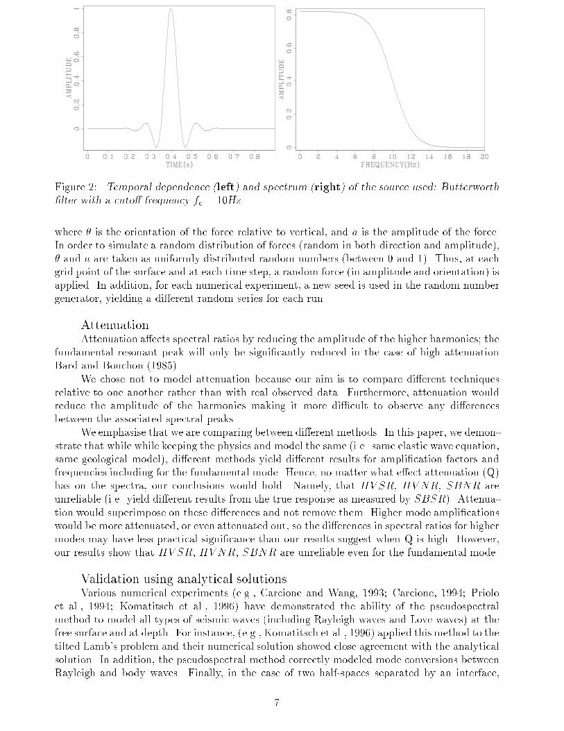
Figure 2: Temporal dependence (left) and spectrum (right) of the source used: Butterworth�lter with a cuto� frequency fc = 10Hz.where � is the orientation of the force relative to vertical, and a is the amplitude of the force.In order to simulate a random distribution of forces (random in both direction and amplitude),� and a are taken as uniformly distributed random numbers (between 0 and 1). Thus, at eachgrid point of the surface and at each time step, a random force (in amplitude and orientation) isapplied. In addition, for each numerical experiment, a new seed is used in the random numbergenerator, yielding a di�erent random series for each run.AttenuationAttenuation a�ects spectral ratios by reducing the amplitude of the higher harmonics; thefundamental resonant peak will only be signi�cantly reduced in the case of high attenuationBard and Bouchon (1985).We chose not to model attenuation because our aim is to compare di�erent techniquesrelative to one another rather than with real observed data. Furthermore, attenuation wouldreduce the amplitude of the harmonics making it more di�cult to observe any di�erencesbetween the associated spectral peaks.We emphasise that we are comparing between di�erent methods. In this paper, we demon-strate that while while keeping the physics and model the same (i.e. same elastic wave equation,same geological model), di�erent methods yield di�erent results for ampli�cation factors andfrequencies including for the fundamental mode. Hence, no matter what e�ect attenuation (Q)has on the spectra, our conclusions would hold. Namely, that HV SR, HV NR, SBNR areunreliable (i.e. yield di�erent results from the true response as measured by SBSR). Attenua-tion would superimpose on these di�erences and not remove them. Higher mode ampli�cationswould be more attenuated, or even attenuated out, so the di�erences in spectral ratios for highermodes may have less practical signi�cance than our results suggest when Q is high. However,our results show that HV SR, HV NR, SBNR are unreliable even for the fundamental mode.Validation using analytical solutionsVarious numerical experiments (e.g., Carcione and Wang, 1993; Carcione, 1994; Prioloet al., 1994; Komatitsch et al., 1996) have demonstrated the ability of the pseudospectralmethod to model all types of seismic waves (including Rayleigh waves and Love waves) at thefree surface and at depth. For instance, (e.g., Komatitsch et al., 1996) applied this method to thetilted Lamb's problem and their numerical solution showed close agreement with the analyticalsolution. In addition, the pseudospectral method correctly modeled mode conversions betweenRayleigh and body waves. Finally, in the case of two half-spaces separated by an interface,7

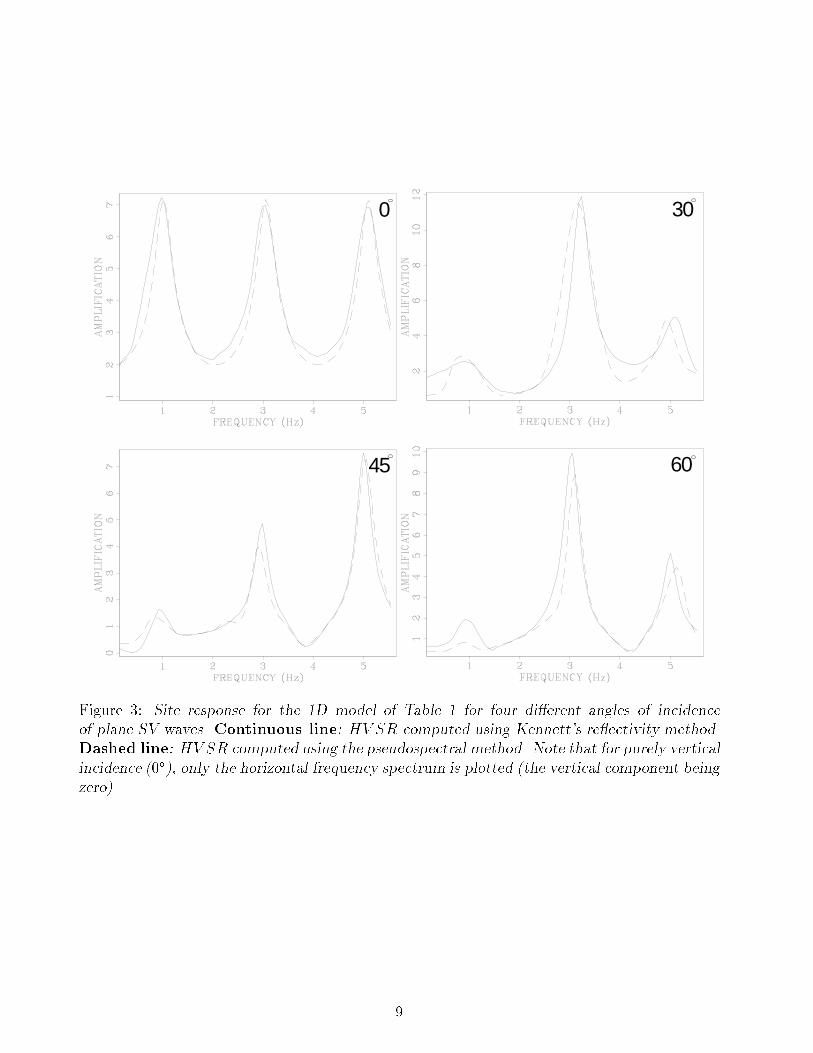
the numerical solution was found to be accurate in the case of re ected and transmitted wavesfrom the interface between the layers with a high contrast in Poisson's ratio.Theoretical response using a simple 1D ModelThe theoretical response of plane SV waves impinging on a single layer overlying a half-space is well known and widely used (e.g., Burridge, 1980; Shearer, 1987; Lermo and Ch�avez-Garc��a, 1993). In order to compare di�erent techniques to determine site ampli�cation, onemust either adopt an empirical approach using seismic recordings or compare these techniquesto an analytical response. Although the analytical response exists only for simple models (1Dwith horizontal layers), it can provide a rough estimation of site response in many cases. Ourpurpose in this section is to validate the modeling technique we used (pseudospectral method)as well as the implementation of the plane SV-waves (c.f. numerical implementation given inthis paper).For waves reverberating within a single (low impedance) surface layer, the position of thespectral peaks for a surface receiver is determined by the vertical travel time within the layer.The eigenfrequencies corresponding to constructive interferences (ampli�cation of waves) aref = (2n+ 1)2T ; n = 0; 1; 2; 3; ::: ; (6)where T is the two-way travel time within the layer. With T = 2H� , where � is the S-wavevelocity in the soil layer and H is the thickness of the layer, one can obtain the well-knownquarter wavelength law f = �(2n+ 1)4H ; n = 0; 1; 2; 3; ::: ; (7)Note that equation (7) is valid only for a single layer over a half-space. From equation (7) andthe parameters we have used (see Table 1), one can expect to obtain peaks of resonance at thefrequencies: 1 Hz, 3 Hz, 5 Hz...HV SR for the 1D model (see Table 1) is computed using the method of generalizedre ection/transmission coe�cients (Kennett and Kerry, 1979) for four di�erent angles of in-cidence. We then compared these ratios with the same ratios (HV SR) computed using thepseudospectral modeling technique (see Fig. 3).Figure 3 shows that for all angles of incidence, the analytical response and our calculationare in good agreement both in terms of amplitude and frequency of resonant peaks. The smalldi�erences observed, notably for the 30� incident angle, are due to the fact that our model is�nite. h (m) � (m=s) � (m=s) � (kg=m3)0-100 690 400 1200100+ 2080 1200 1440Table 1: Description of the 1D model used for computing the theoretical response of one elasticlayer overlying a half-space.Theoretical response using a 2D Model8

0 30

45 60

Figure 3: Site response for the 1D model of Table 1 for four di�erent angles of incidenceof plane SV waves. Continuous line: HV SR computed using Kennett's re ectivity method.Dashed line: HV SR computed using the pseudospectral method. Note that for purely verticalincidence (0�), only the horizontal frequency spectrum is plotted (the vertical component beingzero).9

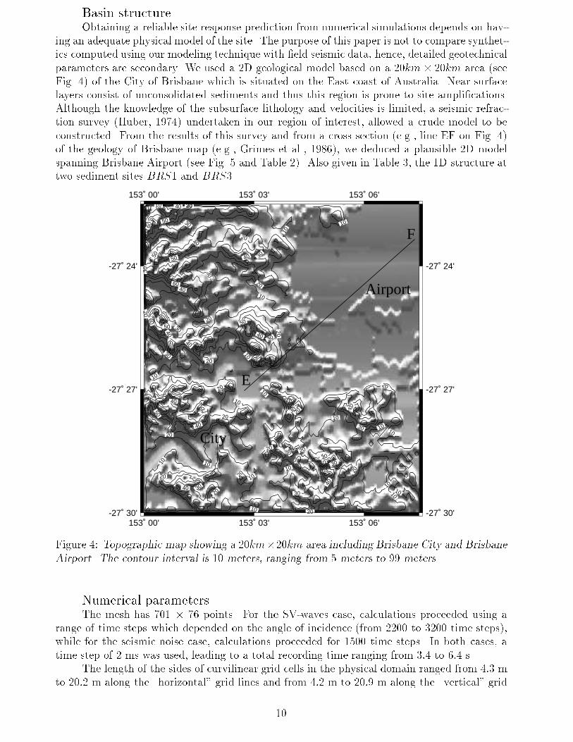
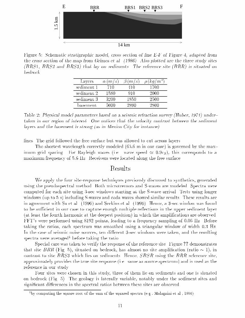
Basin structureObtaining a reliable site response prediction from numerical simulations depends on hav-ing an adequate physical model of the site. The purpose of this paper is not to compare synthet-ics computed using our modeling technique with �eld seismic data, hence, detailed geotechnicalparameters are secondary. We used a 2D geological model based on a 20km � 20km area (seeFig. 4) of the City of Brisbane which is situated on the East coast of Australia. Near surfacelayers consist of unconsolidated sediments and thus this region is prone to site ampli�cations.Although the knowledge of the subsurface lithology and velocities is limited, a seismic refrac-tion survey (Huber, 1974) undertaken in our region of interest, allowed a crude model to beconstructed. From the results of this survey and from a cross section (e.g., line EF on Fig. 4)of the geology of Brisbane map (e.g., Grimes et al., 1986), we deduced a plausible 2D modelspanning Brisbane Airport (see Fig. 5 and Table 2). Also given in Table 3, the 1D structure attwo sediment sites BRS1 and BRS3.10

10

10

1010

10

10

10

10

10

10

10

10

10

10

10

10

1010

20

20

20

20

20

20

20

20

20

2020

2020

20

20

20

20

20

20 20

3030

30

30

3030

30

30

30

30

30

30

30

30

30

30

40

40

40

40

40 4040

40

40

40

40

50

5050

5050

50

60

60

60

153˚ 00'

153˚ 00'

153˚ 03'

153˚ 03'

153˚ 06'

153˚ 06'

-27˚ 30' -27˚ 30'

-27˚ 27' -27˚ 27'

-27˚ 24' -27˚ 24'

E

F

Airport

CityFigure 4: Topographic map showing a 20km�20km area including Brisbane City and BrisbaneAirport. The contour interval is 10 meters, ranging from 5 meters to 99 meters.Numerical parametersThe mesh has 701 � 76 points. For the SV-waves case, calculations proceeded using arange of time steps which depended on the angle of incidence (from 2200 to 3200 time steps),while for the seismic noise case, calculations proceeded for 1500 time steps. In both cases, atime step of 2 ms was used, leading to a total recording time ranging from 3:4 to 6:4 s.The length of the sides of curvilinear grid cells in the physical domain ranged from 4:3 mto 20:2 m along the \horizontal" grid lines and from 4:2 m to 20:9 m along the \vertical" grid10

E FBRR BRS1 BRS2 BRS3

14 km

1.5

kmFigure 5: Schematic stratigraphic model, cross section of line E-F of Figure 4, adapted fromthe cross section of the map from Grimes et al. (1986). Also plotted are the three study sites(BRS1, BRS2 and BRS3) that lay on sediments. The reference site (BRR) is situated onbedrock. Layers � (m=s) � (m=s) � (kg=m3)sediment 1 710 410 1700sediment 2 1580 910 2000sediment 3 3200 1850 2500basement 5000 2890 2800Table 2: Physical model parameters based on a seismic refraction survey (Huber, 1974) under-taken in our region of interest. One notices that the velocity contrast between the sedimentlayers and the basement is strong (as in Mexico City for instance).lines. The grid followed the free surface but was allowed to cut across layers.The shortest wavelength correctly modeled (65:6 m in our case) is governed by the max-imum grid spacing. For Rayleigh waves (i.e. wave speed ' 0:9cS), this corresponds to amaximum frequency of 5:6 Hz. Receivers were located along the free surface.ResultsWe apply the four site-response techniques previously discussed to synthetics, generatedusing the pseudospectral method. Both microtremors and S-waves are modeled. Spectra werecomputed for each site using 3-sec windows starting at the S-wave arrival. Tests using longerwindows (up to 5 s) including S-waves and coda waves showed similar results. These results arein agreement with Su et al. (1996) and Seekins et al. (1996). Hence, a 3-sec window was foundto be su�cient in our case to capture enough multiple re ections in the upper sediment layer(at least the fourth harmonic at the deepest position) in which the ampli�cations are observed.FFT's were performed using 8192 points, leading to a frequency sampling of 0:06 Hz. Beforetaking the ratios, each spectrum was smoothed using a triangular window of width 0:3 Hz.In the case of seismic noise sources, ten di�erent 3-sec windows were taken, and the resultingspectra were averaged1 before taking the ratio.Special care was taken to verify the response of the reference site. Figure ?? demonstratesthat site BRR (Fig. 5), situated on bedrock, has almost no site ampli�cation (ratio � 1), incontrast to site BRS3 which lies on sediments. Hence, SBSR using the BRR reference site,approximately provides the true site response (i.e. same as source spectrum) and is used as thereference in our study.Four sites were chosen in this study, three of them lie on sediments and one is situatedon bedrock (Fig. 5). The geology is laterally variable, notably under the sediment sites andsigni�cant di�erences in the spectral ratios between these sites are observed.1by computing the square root of the sum of the squared spectra (e.g., Malagnini et al., 1996)11

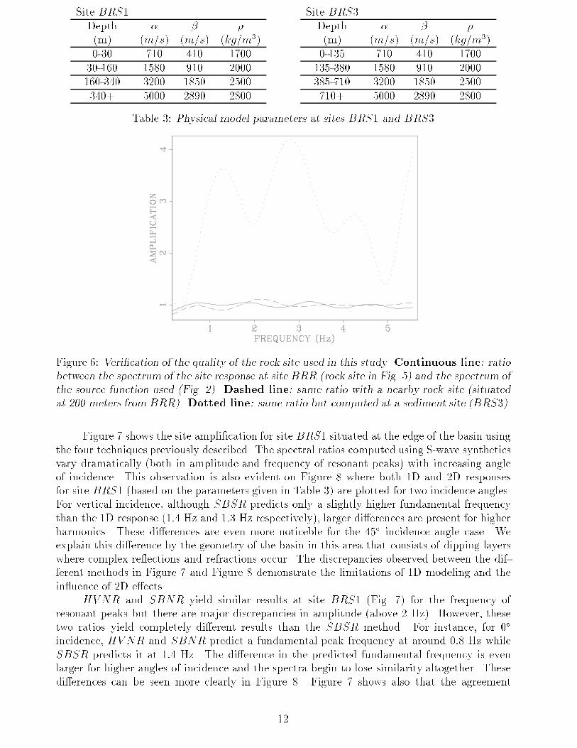
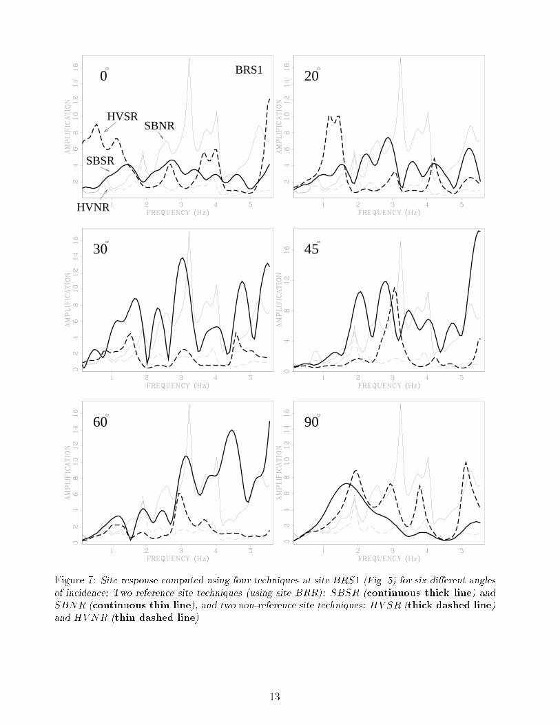
Site BRS1Depth � � �(m) (m=s) (m=s) (kg=m3)0-30 710 410 170030-160 1580 910 2000160-340 3200 1850 2500340+ 5000 2890 2800 Site BRS3Depth � � �(m) (m=s) (m=s) (kg=m3)0-135 710 410 1700135-380 1580 910 2000385-710 3200 1850 2500710+ 5000 2890 2800Table 3: Physical model parameters at sites BRS1 and BRS3Figure 6: Veri�cation of the quality of the rock site used in this study. Continuous line: ratiobetween the spectrum of the site response at site BRR (rock site in Fig. 5) and the spectrum ofthe source function used (Fig. 2). Dashed line: same ratio with a nearby rock site (situatedat 200 meters from BRR). Dotted line: same ratio but computed at a sediment site (BRS3).Figure 7 shows the site ampli�cation for site BRS1 situated at the edge of the basin usingthe four techniques previously described. The spectral ratios computed using S-wave syntheticsvary dramatically (both in amplitude and frequency of resonant peaks) with increasing angleof incidence. This observation is also evident on Figure 8 where both 1D and 2D responsesfor site BRS1 (based on the parameters given in Table 3) are plotted for two incidence angles.For vertical incidence, although SBSR predicts only a slightly higher fundamental frequencythan the 1D response (1:4 Hz and 1:3 Hz respectively), larger di�erences are present for higherharmonics. These di�erences are even more noticeble for the 45� incidence angle case. Weexplain this di�erence by the geometry of the basin in this area that consists of dipping layerswhere complex re ections and refractions occur. The discrepancies observed between the dif-ferent methods in Figure 7 and Figure 8 demonstrate the limitations of 1D modeling and thein uence of 2D e�ects.HV NR and SBNR yield similar results at site BRS1 (Fig. 7) for the frequency ofresonant peaks but there are major discrepancies in amplitude (above 2 Hz). However, thesetwo ratios yield completely di�erent results than the SBSR method. For instance, for 0�incidence, HV NR and SBNR predict a fundamental peak frequency at around 0:8 Hz whileSBSR predicts it at 1:4 Hz. The di�erence in the predicted fundamental frequency is evenlarger for higher angles of incidence and the spectra begin to lose similarity altogether. Thesedi�erences can be seen more clearly in Figure 8. Figure 7 shows also that the agreement12

0

HVSR

SBSR

SBNR

BRS1

HVNR

20

30 45

60 90

Figure 7: Site response computed using four techniques at site BRS1 (Fig. 5) for six di�erent anglesof incidence; Two reference site techniques (using site BRR): SBSR (continuous thick line) andSBNR (continuous thin line), and two non-reference site techniques: HVSR (thick dashed line)and HVNR (thin dashed line). 13

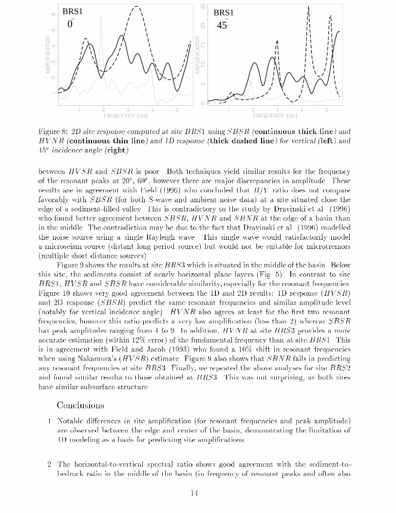
0BRS1

45BRS1

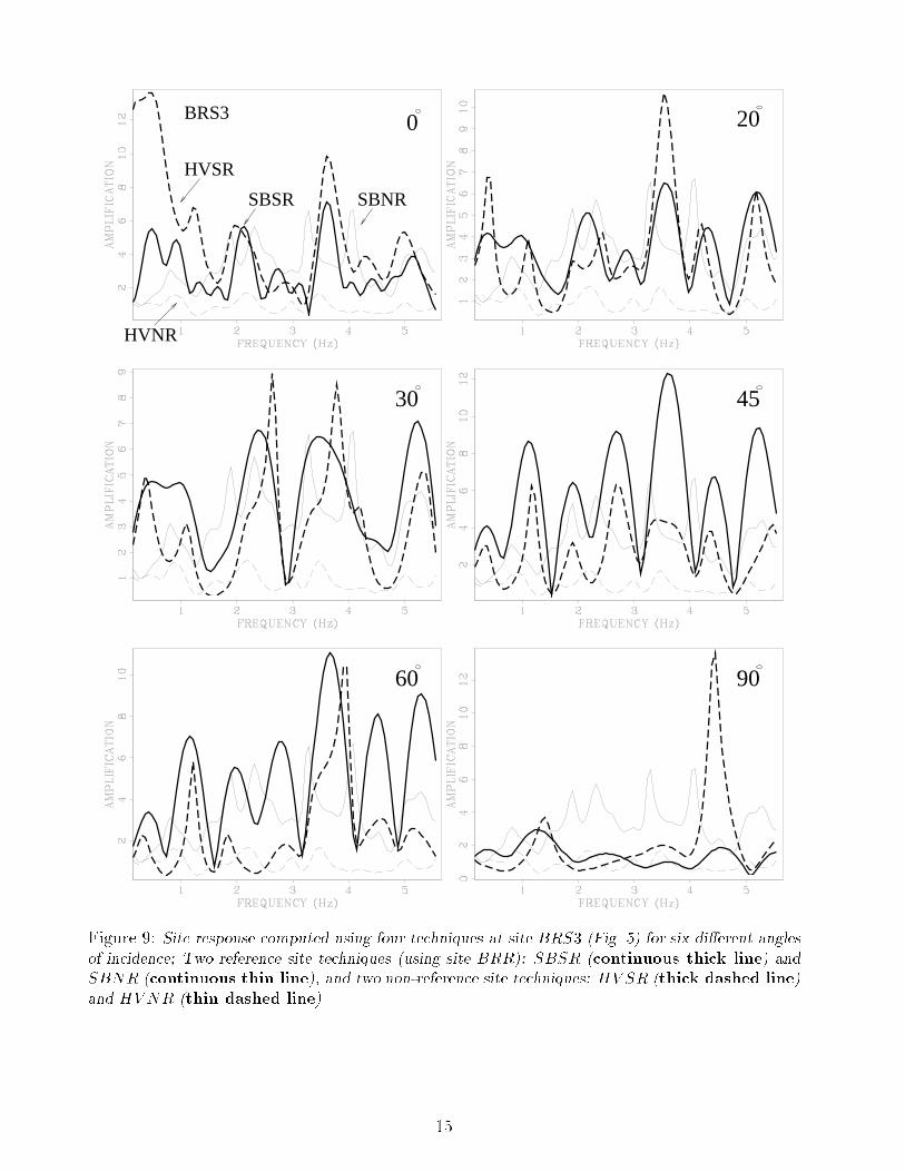
Figure 8: 2D site response computed at site BRS1 using SBSR (continuous thick line) andHV NR (continuous thin line) and 1D response (thick dashed line) for vertical (left) and45� incidence angle (right).between HV SR and SBSR is poor. Both techniques yield similar results for the frequencyof the resonant peaks at 20�, 60�, however there are major discrepancies in amplitude. Theseresults are in agreement with Field (1996) who concluded that H=V ratio does not comparefavorably with SBSR (for both S-wave and ambient noise data) at a site situated close theedge of a sediment-�lled valley. This is contradictory to the study by Dravinski et al. (1996)who found better agreement between SBSR, HV NR and SBNR at the edge of a basin thanin the middle. The contradiction may be due to the fact that Dravinski et al. (1996) modelledthe noise source using a single Rayleigh wave. This single wave would satisfactorily modela microseism source (distant long period source) but would not be suitable for microtremors(multiple short distance sources).Figure 9 shows the results at siteBRS3 which is situated in the middle of the basin. Belowthis site, the sediments consist of nearly horizontal plane layers (Fig. 5). In contrast to siteBRS1, HV SR and SBSR have considerable similarity, especially for the resonant frequencies.Figure 10 shows very good agreement between the 1D and 2D results: 1D response (HV SR)and 2D response (SBSR) predict the same resonant frequencies and similar amplitude level(notably for vertical incidence angle). HV NR also agrees at least for the �rst two resonantfrequencies, however this ratio predicts a very low ampli�cation (less than 2) whereas SBSRhas peak amplitudes ranging from 4 to 9. In addition, HV NR at site BRS3 provides a moreaccurate estimation (within 12% error) of the fundamental frequency than at site BRS1. Thisis in agreement with Field and Jacob (1993) who found a 10% shift in resonant frequencieswhen using Nakamura's (HV SR) estimate. Figure 9 also shows that SBNR fails in predictingany resonant frequencies at site BRS3. Finally, we repeated the above analyses for site BRS2and found similar results to those obtained at BRS3. This was not surprising, as both siteshave similar subsurface structure.Conclusions1. Notable di�erences in site ampli�cation (for resonant frequencies and peak amplitude)are observed between the edge and center of the basin, demonstrating the limitation of1D modeling as a basis for predicting site ampli�cations.2. The horizontal-to-vertical spectral ratio shows good agreement with the sediment-to-bedrock ratio in the middle of the basin (in frequency of resonant peaks and often also14

0

HVNR

HVSR

SBSR

BRS3

SBNR

20

30 45

60 90

Figure 9: Site response computed using four techniques at site BRS3 (Fig. 5) for six di�erent anglesof incidence; Two reference site techniques (using site BRR): SBSR (continuous thick line) andSBNR (continuous thin line), and two non-reference site techniques: HVSR (thick dashed line)and HVNR (thin dashed line). 15

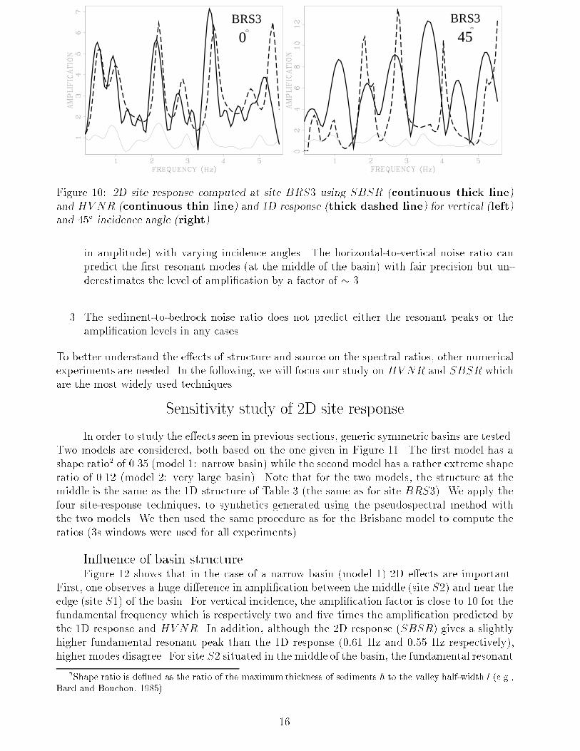
0BRS3

45BRS3

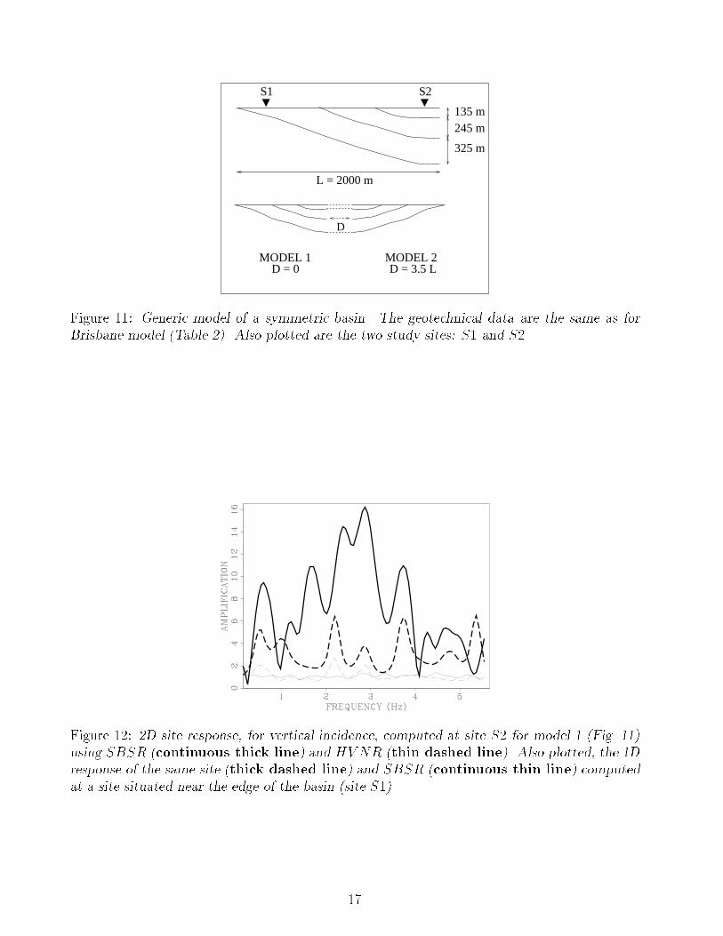
Figure 10: 2D site response computed at site BRS3 using SBSR (continuous thick line)and HV NR (continuous thin line) and 1D response (thick dashed line) for vertical (left)and 45� incidence angle (right).in amplitude) with varying incidence angles. The horizontal-to-vertical noise ratio canpredict the �rst resonant modes (at the middle of the basin) with fair precision but un-derestimates the level of ampli�cation by a factor of � 3.3. The sediment-to-bedrock noise ratio does not predict either the resonant peaks or theampli�cation levels in any cases.To better understand the e�ects of structure and source on the spectral ratios, other numericalexperiments are needed. In the following, we will focus our study on HV NR and SBSR whichare the most widely used techniques.Sensitivity study of 2D site responseIn order to study the e�ects seen in previous sections, generic symmetric basins are tested.Two models are considered, both based on the one given in Figure 11. The �rst model has ashape ratio2 of 0.35 (model 1: narrow basin) while the second model has a rather extreme shaperatio of 0.12 (model 2: very large basin). Note that for the two models, the structure at themiddle is the same as the 1D structure of Table 3 (the same as for site BRS3). We apply thefour site-response techniques, to synthetics generated using the pseudospectral method withthe two models. We then used the same procedure as for the Brisbane model to compute theratios (3s windows were used for all experiments).In uence of basin structureFigure 12 shows that in the case of a narrow basin (model 1) 2D e�ects are important.First, one observes a huge di�erence in ampli�cation between the middle (site S2) and near theedge (site S1) of the basin. For vertical incidence, the ampli�cation factor is close to 10 for thefundamental frequency which is respectively two and �ve times the ampli�cation predicted bythe 1D response and HV NR. In addition, although the 2D response (SBSR) gives a slightlyhigher fundamental resonant peak than the 1D response (0:61 Hz and 0:55 Hz respectively),higher modes disagree. For site S2 situated in the middle of the basin, the fundamental resonant2Shape ratio is de�ned as the ratio of the maximum thickness of sediments h to the valley half-width l (e.g.,Bard and Bouchon, 1985). 16

MODEL 1 MODEL 2

D

135 m245 m

325 m

L = 2000 m

D = 0 D = 3.5 L

S1 S2

Figure 11: Generic model of a symmetric basin. The geotechnical data are the same as forBrisbane model (Table 2). Also plotted are the two study sites: S1 and S2.

Figure 12: 2D site response, for vertical incidence, computed at site S2 for model 1 (Fig. 11)using SBSR (continuous thick line) and HV NR (thin dashed line). Also plotted, the 1Dresponse of the same site (thick dashed line) and SBSR (continuous thin line) computedat a site situated near the edge of the basin (site S1).17

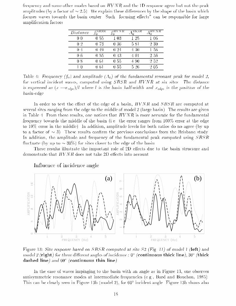
frequency and some other modes based on HV NR and the 1D response agree but not the peakamplitudes (by a factor of � 2:5). We explain these di�erences by the shape of the basin whichfocuses waves towards the basin center. Such \focusing e�ects" can be responsible for largeampli�cation factors. Distance fSBSR0 fHVNR0 ASBSR0 AHVNR00.0 0.55 1.03 1.25 1.060.2 0.73 0.36 5.81 2.300.4 0.49 0.24 4.30 1.560.6 0.55 0.43 4.01 2.560.8 0.61 0.55 4.90 2.521.0 0.61 0.55 5.26 2.05Table 4: Frequency (f0) and amplitude (A0) of the fundamental resonant peak for model 2,for vertical incident waves, computed using SBSR and HV NR at six sites. The distanceis expressed as (x � xedge)=l where l is the basin half-width and xedge is the position of thebasin-edge.In order to test the e�ect of the edge of a basin, HV NR and SBSR are computed atseveral sites ranging from the edge to the middle of model 2 (large basin). The results are givenin Table 4. From these results, one notices that HV NR is more accurate for the fundamentalfrequency towards the middle of the basin (i.e. the error ranges from 100% error at the edgeto 10% error in the middle). In addition, amplitude levels for both ratios do no agree (by upto a factor of � 3). These results con�rm the previous conclusions from the Brisbane study.In addition, the amplitude and frequency of the fundamental peak computed using SBSR uctuate (by up to � 30%) for sites closer to the edge of the basin.These results illustrate the important role of 2D e�ects due to the basin structure anddemonstrate that HV NR does not take 2D e�ects into account .In uence of incidence angle(a) (b)

Figure 13: Site response based on SBSR computed at site S2 (Fig. 11) of model 1 (left) andmodel 2 (right) for three di�erent angles of incidence : 0� (continuous thick line), 30� (thickdashed line) and 60� (continuous thin line) .In the case of waves impinging to the basin with an angle as in Figure 13, one observesantisymmetric resonance modes at intermediate frequencies (e.g., Bard and Bouchon, 1985).This can be clearly seen in Figure 13b (model 2), for 60� incident angle. Figure 13b shows also18

that the position of resonant peaks is similar for 0� and 60� degrees and that the amplitude of thefundamental mode is maximum for vertical incidence. In contrast, in the case of a narrow basin(see Figure 13a) the problem is much more complex: discrepancies in amplitude and positionof the resonant peaks can be observed at di�erent incidence angles. These results show thatthe position of the source greatly in uences site response for narrow basins. We explain thesediscrepancies as due to the geometry of the basin which consists of steeply dipping layers.ConclusionsOur simulation based approach to determine and study site ampli�cation, using the pseu-dospectral modeling method, has provided new information about the reliability of four widelyused site-response estimation techniques. The sediment-to-bedrock ratio provided the \true"response in all experiments (the reference site was chosen such that its spectrum was approxi-mately equal to the source spectrum).The limits of applicability of these techniques were tested using �rst a 2D basin modelin the Brisbane area (Australia). We �nd that the horizontal-to-vertical spectral ratio agreesbetter (in resonant frequencies and amplitude) with the sediment-to-bedrock spectral ratio inthe middle of the basin than at the edge. The horizontal-to-vertical noise ratio predicts the �rstresonant mode in the middle of the basin but underestimates the peak amplitude by a factorof approximately 3. The sediment-to-bedrock noise ratio shows poor correlation with the otherratios.In order to better understand the in uence of 2D structure on the spectral ratios, twoother models (symmetric basins) were tested. We �nd that in the case of a large basin (with ashape ratio of 0:12, i.e almost at layers) the horizontal-to-vertical noise ratio provides a fairestimation (within 10% error) for the fundamental frequency of resonance, but this ratio isunable to predict either the higher modes or the ampli�cation levels. In the case of a narrowerbasin (with a shape ratio of 0:35) the horizontal-to-vertical noise ratio yields a similar predictionas the 1D response for the resonant frequencies but underestimates the ampli�cation (by a factorof approximately 2:5). However, these two estimates are far from the \true" response in thecase of a narrow basin.Finally, these experiments showed that 2D e�ects such as basin edge e�ects and focusinge�ects greatly in uence the site response. We noted strong variations of the site ampli�cationspectrum (frequencies and amplitude) as a function of basin structure and incidence angle ofthe incoming waves particularly at the edge of a basin.In summary, estimation of site ampli�cation spectra using observational methods yieldunreliable or incorrect results when subsurface basin structure is present.AcknowledgmentsThe authors would like to thank Russell Cuthbertson, Dimitri Komatitsch, and Jos�e Carcionefor very fruitful discussions. Thanks also to Edward Field for his constructive comments which havegreatly improved this manuscript.This research was funded by the Australian Research Council. Supplementary funding wasprovided by the University of Queensland and by the sponsors of the Seismic Simulation Project andQUAKES (Amoco, Silicon Graphics Inc., Cairns City Council).Principle computations were made using QUAKES 8 processor Silicon Graphics Origin2000 andthe 16 processor Silicon Graphics Power Challenge of the University of Queensland High PerformanceComputing Unit (HPCU). 19

ReferencesBard, P.-Y. (1995). E�ects of surface geology on ground motion: Recent results and remainingissues. In Proc. of the 10th European Conference on Earthquake Engineering, pp. 305{323.Rotterdam.Bard, P.-Y. and M. Bouchon (1985). The two-dimensional resonance of sediment-�lled valleys.Bull. Seis. Soc. Am. 75, 519{541.Borcherdt, R. D. (1970). E�ects of local geology on ground motion near San Francisco Bay.Bull. Seis. Soc. Am. 60, 29{61.Burridge, R. (1980). Soil ampli�cation of plane seismic waves. Phys. Earth Int. 22, 122{136.Carcione, J. M. (1994). The wave equation in generalized coordinates. Geophysics 59, 1911{1919.Carcione, J. M. and J. P. Wang (1993). A Chebyshev collocation method for the elastody-namic equation in generalized coordinates. Bull. Seis. Soc. Am. 2, 269{290.Clitheroe, G. M. and J. J. Taber (1995). Assessing earthquake site response using mi-crotremors: a case study in Wellington city, New Zealand. In Proc. of the Paci�c Con-ference on Earthquake Engineering, pp. 247{256. Melbourne, Australia, November 1995.Darragh, R. B. and A. F. Shakal (1991). The site response of two rock and soil station pairsto strong and weak ground motion. Bull. Seis. Soc. Am. 81, 1885{1899.Dravinski, M., G. Ding, and K. L. Wen (1996). Analysis of spectral ratios for estimatingground motion in deep basins. Bull. Seis. Soc. Am. 86, 646{654.Field, E. H. (1996). Spectral ampli�cation in a sediment-�lled valley exhibiting clear basin-edge-induced waves. Bull. Seis. Soc. Am. 86, 991{1005.Field, E. H. and K. H. Jacob (1993). The theoretical response of sedimentary layers toambient seismic noise. Geophys. Res. Lett. 24, 2925{2928.Field, E. H. and K. H. Jacob (1995). A comparison and test of various site-response estimationtechniques, including three that are not reference-site dependent. Bull. Seis. Soc. Am. 85,1127{1143.Grimes, K. G., L. C. Cran�eld, P. J. T. Donchack, L. J. Hutton, and M. R. Jones (1986).Australia 1:100 000 Geological Series, sheet 9543. Queensland: Department of Mines.Hough, S. E., R. D. Borcherdt, P. A. Friberg, R. Busby, E. H. Field, and K. H. Jacob (1990).The role of sediment-induced ampli�cation in the collapse of the Nimitz freeway duringthe October 17, 1989 Loma Prieta earthquake. Nature 344, 853{855.Huber, R. D. (1974). Schultz canal seismic refraction survey. Geological Survey of QueenslandRecord 1974/9 (unpublished).Jarpe, S. P., C. H. Cramer, B. E. Tucker, and A. F. Shakal (1988). A comparison of observa-tions of ground response to weak and strong motion at Coalinga, California. Bull. Seis.Soc. Am. 78, 421{435.Kennett, B. L. N. and N. J. Kerry (1979). Seismic waves in a strati�ed half space. Geophys.J. Roy. Astr. Soc. 57, 557{583.Komatitsch, D., F. Coutel, and P. Mora (1996). Tensorial formulation of the wave-equationfor modeling curved interfaces. Geophys. J. Int. 127, 156{168.20

Koslo�, D. and H. Tal-Ezer (1993). A modi�ed Chebyshev pseudospectral method with anO(N�1) time step restriction. J. Comput. Phys. 104, 457{469.Lachet, C. and P.-Y. Bard (1994). Numerical and theoretical investigations on the possibilitiesand limitations of Nakamura's technique. J. Phys. Earth 42, 377{397.Lachet, C., D. Hazfeld, P.-Y. Bard, N. Theodulidis, C. Papaioannou, and A. Savvaidis (1996).Site e�ects and microzonation in the city of Thessaloniki (Greece) comparison of di�erentapproaches. Bull. Seis. Soc. Am. 86, 1692{1703.Lermo, J. and F. J. Ch�avez-Garc��a (1993). Site e�ect evaluation using spectral ratios withonly one station. Bull. Seis. Soc. Am. 83, 1574{1594.Lermo, J. and F. J. Ch�avez-Garc��a (1994). Are microtremors useful in site response evalua-tion? Bull. Seis. Soc. Am. 84, 1350{1364.Malagnini, L., P. Tricarico, A. Rovelli, R. B. Herrmann, S. Opice, G. Biella, and R. de Franco(1996). Explosion, earthquake, and ambient noise recordings in a Pliocene sediment-�lled valley: inferences on seismic response properties by reference- and non-reference-sitetechniques. Bull. Seis. Soc. Am. 86, 670{682.Margheriti, L., L. Wennerberg, and J. Boatwright (1994). A comparison of coda and S-wavespectral ratios as estimates of site response in the Southern San Francisco Bay area. Bull.Seis. Soc. Am. 84, 1815{1830.Nakamura, Y. (1989). A method for dynamic characteristics estimation of subsurface usingmicrotremor on the ground surface. QR Railway Tech. Res. Inst. 30, 25{33.Ohta, Y., H. Kagami, N. Goto, and K. Kudo (1978). Observation of 1- to 5-second mi-crotremors and their application to earthquake engineering. Part I: comparison withlong-period accelerations at the Tokachi-Oki earthquake of 1968. Bull. Seis. Soc. Am. 68,767{779.Priolo, E., J. M. Carcione, and G. Seriani (1994). Numerical simulation of interface wavesby high order spectral modeling techniques. Bull. Seis. Soc. Am. 95, 681{693.Seekins, L. C., L. Wennerberg, L. Margheriti, and H. P. Liu (1996). Site ampli�cation at �velocations in San Francisco, California: a comparison of S waves, codas, and microtremors.Bull. Seis. Soc. Am. 86, 627{635.Shearer, P. M. (1987). Surface and near-surface e�ects on seismic waves theory and boreholeseismometer results. Bull. Seis. Soc. Am. 77, 1168{1196.Singh, S. K., J. Lermo, T. Dominguez, M. Ordaz, J. M. Espinosa, E. Mena, and R. Quass(1988). The Mexico earthquake of September 19, 1985{A study of seismic waves in theValley of Mexico with respect to a hill zone site. Earthq. Spectra. 4, 653{673.Steidtl, J., A. G. Tumarkin, and R. J. Archuleta (1996). What is a reference site? Bull. Seis.Soc. Am. 86, 1733{1748.Su, F., J. G. Anderson, J. N. Brune, and Y. Zeng (1996). A comparison of direct S-wave andcoda-wave site ampli�cation determined from aftershocks of the Little Skull mountainearthquake. Bull. Seis. Soc. Am. 86, 1006{1018.Virieux, J. (1986). P-SV wave propagation in heterogeneous media. Geophysics 51, 889{901.Yamanaka, H., M. Takemura, H. Ishida, and M. Niwa (1994). Characteristics of long-periodmicrotremors and their applicability in exploration of deep sedimentary layers. Bull. Seis.Soc. Am. 84, 1831{1841. 21