simulation of the june 11, 2010, flood along the little missouri … · front cover, downstream...

U.S. Department of the InteriorU.S. Geological Survey

Scientific Investigations Report 2013–5056

Prepared in cooperation with the U.S. Department of Agriculture—Forest Service

Simulation of the June 11, 2010, Flood Along the Little Missouri River near Langley, Arkansas, Using a Hydrologic Model Coupled to a Hydraulic Model

Front cover, Downstream view of the Little Missouri River watershed near the Albert Pike Recreation Area, Arkansas. The surface represents maximum flood stage and colors represent maximum velocity. Vertical exaggeration is 2x.

Back cover, Downstream view of the Little Missouri River watershed near the Albert Pike Recreation Area, Arkansas.


By Drew A. Westerman and Brian R. Clark

Prepared in cooperation with the U.S. Department of Agriculture—Forest Service

Scientific Investigations Report 2013–5056

U.S. Department of the InteriorU.S. Geological Survey

U.S. Department of the InteriorSALLY JEWELL, Secretary

U.S. Geological SurveySuzette M. Kimball, Acting Director

U.S. Geological Survey, Reston, Virginia: 2013

This and other USGS information products are available at http://store.usgs.gov/

U.S. Geological Survey Box 25286, Denver Federal Center Denver, CO 80225

To learn about the USGS and its information products visit http://www.usgs.gov/ 1-888-ASK-USGS

Any use of trade, product, or firm names is for descriptive purposes only and does not imply endorsement by the U.S. Government.

Although this report is in the public domain, permission must be secured from the individual copyright owners to reproduce any copyrighted materials contained within this report.

Suggested citation:Westerman, D.A., and Clark, B.R., 2013, Simulation of the June 11, 2010, flood along the Little Missouri River near Langley, Arkansas, using a hydrologic model coupled to a hydraulic model: U.S. Geological Survey Scientific Investigations Report 2013–5056, 34 p., http://pubs.usgs.gov/sir/2013/5056/.

iii

ContentsAbstract ..........................................................................................................................................................1Introduction ....................................................................................................................................................1Purpose and Scope ......................................................................................................................................4Precipitation-Runoff Hydrologic Model Development and Calibration ...............................................4

Development .........................................................................................................................................4Model Framework .......................................................................................................................4Precipitation Depth and Distribution .......................................................................................5Precipitation Transformation ....................................................................................................8Precipitation Losses ...................................................................................................................8Base Flow .....................................................................................................................................8Channel Routing ........................................................................................................................10

Calibration of Hydrologic Model .....................................................................................................10Precipitation Characteristics ..................................................................................................13Streamflows at the Langley Streamgage .............................................................................13Streamflows at Indirect Discharge Measurement Locations ...........................................18

Simulated Peak Streamflows and Timing ...............................................................................................18One-Dimensional Unsteady-State Hydraulic Model Development and Calibration ........................20

Development .......................................................................................................................................20Model Framework .....................................................................................................................20Manning’s Roughness Coefficients .......................................................................................21Boundary and Initial Conditions .............................................................................................21

Calibration of 1-D Hydraulic Model ................................................................................................21Simulated Water Depth, Rate of Rise, and Velocities ...........................................................................22Sensitivity Analysis .....................................................................................................................................23Model Limitations and Model Comparison .............................................................................................26Summary .......................................................................................................................................................27References Cited .........................................................................................................................................27Appendix 1. High-Water Marks Used to Calibrate the One-Dimensional Hydraulic

Model of the Little Missouri River Watershed, Arkansas ..........................................31

Figures 1. Maps showing locations of the A, Little Missouri River and tributaries,

watershed and model boundaries, and streamgage and indirect discharge measurement locations; B, Albert Pike Recreation Area campgrounds and indirect discharge measurement locations in the immediate vicinity of the Albert Pike Recreation Area ......................................................................................................2

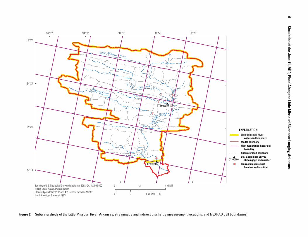
2. Map showing subwatersheds of the Little Missouri River, Arkansas, streamgage and indirect discharge measurement locations, and NEXRAD cell boundaries ..............6

3. Map showing subwatersheds of the Little Missouri River, Arkansas, and modeled stream reaches ............................................................................................................................7

4. Map showing Arkansas annual precipitation normal for 1981–2010 ................................14

iv

5. Map showing cumulative storm precipitation totals for the June 11, 2010, flood event from National Oceanic and Atmospheric Administration NEXRAD (next-generation radar) for the period from 4:00 a.m. on June 10 to 6:00 a.m. on June 12, 2010 ..............................................................................................................................15

6. Map showing cumulative subwatershed precipitation input for the precipitation- runoff hydrologic model from 2:00 a.m. on June 10 to 2:00 p.m. on June 12, 2010 ..........16

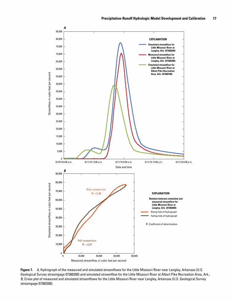
7. Graphs showing A, hydrograph of the measured and simulated streamflows for the Little Missouri River near Langley, Arkansas (U.S. Geological Survey streamgage 07360200) and simulated streamflow for the Little Missouri River at Albert Pike Recreation Area, Ark.; B, Cross plot of measured and simulated streamflows for the Little Missouri River near Langley, Arkansas (U.S. Geological Survey streamgage 07360200) .................................................................................................17

8. Simulated hydrographs for selected locations within the Little Missouri watershed, Arkansas ................................................................................................................19

9. Maps showing the comparison of water depths simulated by the one- dimensional unsteady-state hydraulic model for the Little Missouri River watershed, Arkansas, for the June 11, 2010, flood event at: A. 10:00 p.m. on June 10, B. 2:00 a.m. and C. 3:00 a.m. on June 11, and D. maximum depth at approximately 4:05 a.m. on June 11 ........................................................................................24

10. Maps showing the comparison of water velocities simulated by the one- dimensional unsteady-state hydraulic model for the Little Missouri watershed, Arkansas, for the June 11, 2010, flood event at: A. 10:00 p.m. on June 10, B. 2:00 a.m. and C. 3:00 a.m. on June 11, and D. maximum velocity at approximately 4:05 a.m. on June 11 ........................................................................................25

Tables 1. Subwatershed characteristics and calibrated parameters for the Little Missouri

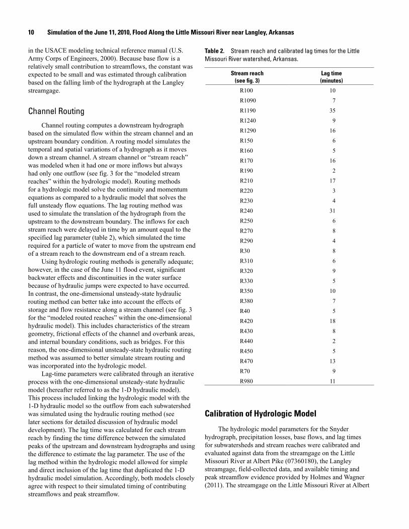
River watershed, Arkansas ........................................................................................................9 2. Stream reach and calibrated lag times for the Little Missouri River watershed,

Arkansas .....................................................................................................................................10 3. Summary of watershed, peak streamflows, hydraulic properties, and simulated

streamflow characteristics for selected locations for the Little Missouri River watershed, Arkansas ................................................................................................................12

4. Comparison of surveyed high-water marks and simulated water-surface elevations for the Little Missouri River watershed, Arkansas ...........................................22

5. Summary of simulated hydraulic properties at the flood peak corresponding to the indirect discharge measurement locations for the Little Missouri River watershed, Arkansas ................................................................................................................23

v

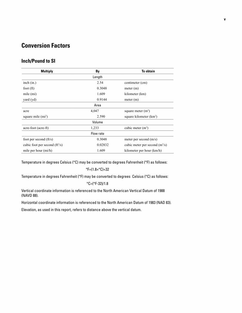
Conversion Factors

Inch/Pound to SI

Multiply By To obtain

Length

inch (in.) 2.54 centimeter (cm)foot (ft) 0.3048 meter (m)mile (mi) 1.609 kilometer (km)yard (yd) 0.9144 meter (m)

Area

acre 4,047 square meter (m2)square mile (mi2) 2.590 square kilometer (km2)

Volume

acre-foot (acre-ft) 1,233 cubic meter (m3)Flow rate

foot per second (ft/s) 0.3048 meter per second (m/s)cubic foot per second (ft3/s) 0.02832 cubic meter per second (m3/s)mile per hour (mi/h) 1.609 kilometer per hour (km/h)

Temperature in degrees Celsius (°C) may be converted to degrees Fahrenheit (°F) as follows:

°F=(1.8×°C)+32

Temperature in degrees Fahrenheit (°F) may be converted to degrees Celsius (°C) as follows:

°C=(°F-32)/1.8

Vertical coordinate information is referenced to the North American Vertical Datum of 1988 (NAVD 88).

Horizontal coordinate information is referenced to the North American Datum of 1983 (NAD 83).

Elevation, as used in this report, refers to distance above the vertical datum.


By Drew A. Westerman and Brian R. Clark

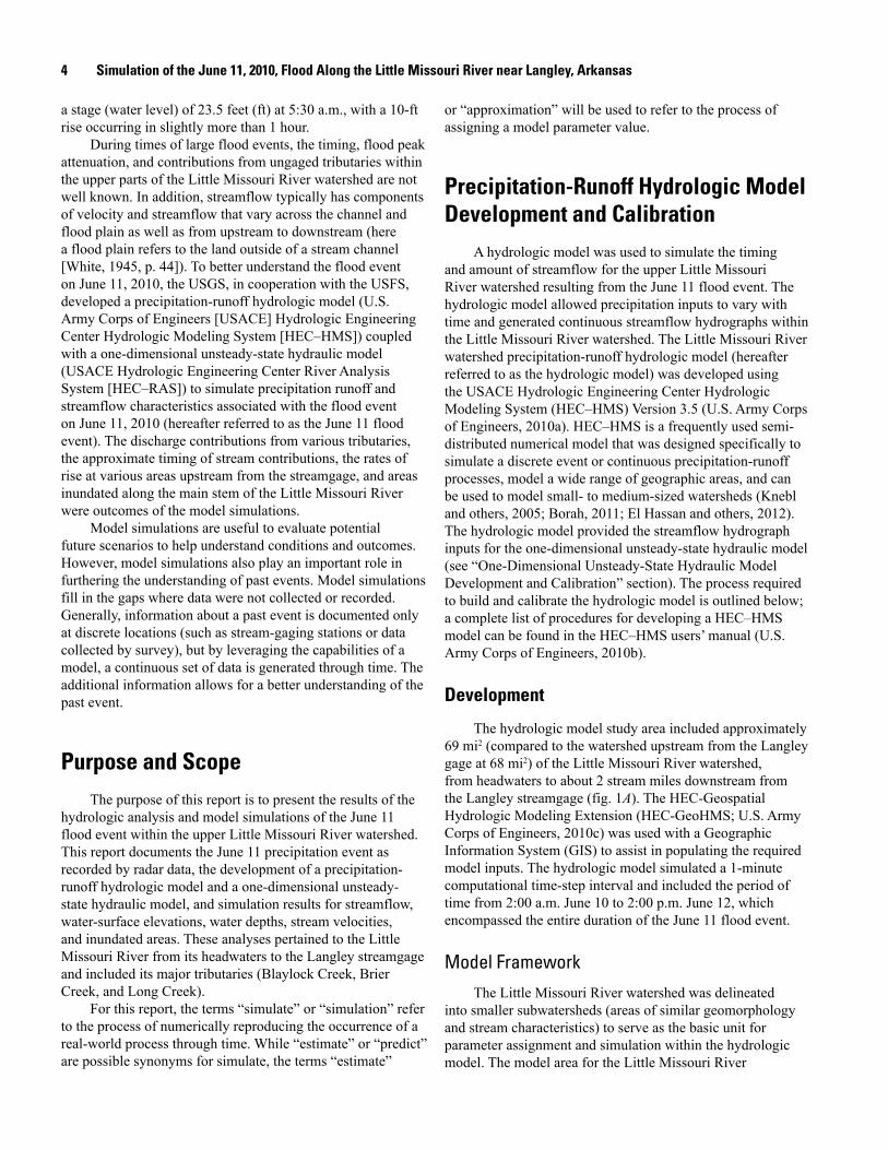
AbstractA substantial flood event occurred on June 11, 2010,

causing the Little Missouri River to flow over much of the adjacent land area, resulting in catastrophic damages. Twenty fatalities occurred and numerous automobiles, cabins, and recreational vehicles were destroyed within the U.S. Department of Agriculture—Forest Service Albert Pike Recreation Area, at a dispersed campsite area in the surrounding Ouachita National Forest lands, and at a nearby privately owned camp. The Little Missouri River streamgage near Langley, Arkansas, reached a record streamflow of 70,800 cubic feet per second and a stage (water level) of 23.5 feet at 5:30 a.m., with a 10-foot rise occurring in slightly more than 1 hour.

To better understand the flood event on June 11, 2010, the U.S. Geological Survey, in cooperation with the U.S. Department of Agriculture—Forest Service, developed a precipitation-runoff hydrologic model, U.S. Army Corps of Engineers Hydrologic Engineering Center Hydrologic Modeling System (HEC–HMS), coupled with a one-dimensional unsteady-state hydraulic model, U.S. Army Corps of Engineers Hydrologic Engineering Center River Analysis System (HEC–RAS), to simulate precipitation runoff and streamflow characteristics along the Little Missouri River and at various tributaries within the 68-square mile watershed upstream from the Langley streamgage.

Within the proximity of two campgrounds, the Little Missouri River just downstream from the confluence of Brier Creek had a peak simulated streamflow of 49,300 cubic feet per second at 4:08 a.m.; the simulated streamflow stayed within 500 cubic feet per second of the peak for nearly 15 minutes. The simulated water surface increased an average of 0.5 feet every 5 minutes for a total of 2 hours, with a maximum rate of rise of 2 feet in 15 minutes. The Little Missouri River just downstream from the confluence of Brier Creek had a peak simulated water-surface elevation of 935.0 feet, a maximum water depth of 22.2 feet, and a maximum stream channel velocity of 12.6 feet per second at 4:15 a.m.

The results from the precipitation-runoff hydrologic model, the one-dimensional unsteady-state hydraulic model,

and a separate two-dimensional model developed as part of a coincident study, each complement the other in terms of streamflow timing, water-surface elevations, and velocities propagated by the June 11, 2010, flood event. The simulated grids for water depth and stream velocity from each model were directly compared by subtracting the one-dimensional hydraulic model grid from the two-dimensional model grid. The absolute mean difference for the simulated water depth was 0.9 foot. Additionally, the absolute mean difference for the simulated stream velocity was 1.9 feet per second.

Introduction The Little Missouri River (fig. 1) and tributaries are

located in southwestern Arkansas, within the southern Ouachita Mountains: a series of east-west trending, complexly folded, and faulted sedimentary rocks. The Little Missouri River watershed, in general, is remote, has steep sloping valleys, and high stream gradients. Periods of heavy precipitation are common (Williams and others, 2003), with the potential to create flash floods with ‘relatively large flows’ (O’Connor and Costa, 2003).

A substantial flood event occurred on June 11, 2010, causing the Little Missouri River to flow over much of the adjacent land area, resulting in catastrophic damages. Twenty fatalities occurred and numerous automobiles, cabins, and recreational vehicles were destroyed within the U.S. Department of Agriculture—Forest Service (USFS) Albert Pike Recreation Area (Albert Pike) that consists of four campground areas, at a dispersed campsite area in the surrounding Ouachita National Forest lands, and at a nearby privately owned camp (Camp Albert Pike). The U.S. Geological Survey (USGS) operates a streamgage, Little Missouri River near Langley, Arkansas (USGS 07360200, fig. 1A; hereafter referred to as the Langley streamgage), located at the Highway 84 crossing approximately 8.5 miles (mi) downstream from Albert Pike. The streamgage measures runoff for approximately 68 square miles (mi2) of the upper part of the Little Missouri River watershed and has been in operation since 1996. The Little Missouri River reached a record streamflow of 70,800 cubic feet per second (ft3/s) and

2

Simulation of the June 11, 2010, Flood Along the Little M

issouri River near Langley, Arkansas

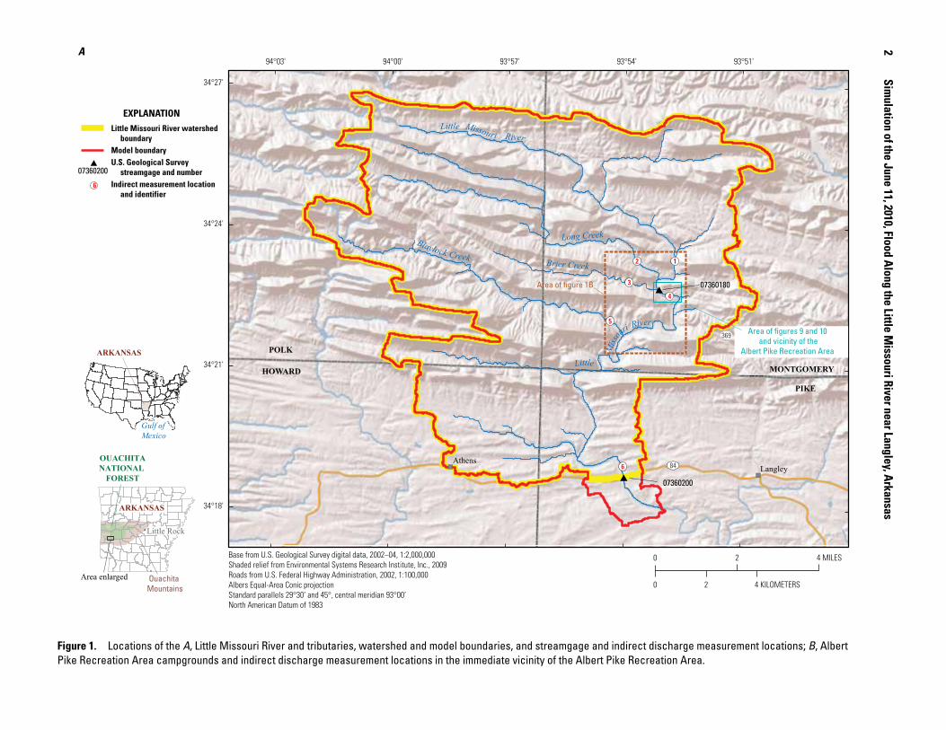
Figure 1. Locations of the A, Little Missouri River and tributaries, watershed and model boundaries, and streamgage and indirect discharge measurement locations; B, Albert Pike Recreation Area campgrounds and indirect discharge measurement locations in the immediate vicinity of the Albert Pike Recreation Area.

")

")Athens

Langley

POLK

PIKE

MONTGOMERYHOWARD

U369

U84

Gulf ofMexico

ARKANSAS

Area of figures 9 and 10 and vicinity of the

Albert Pike Recreation Area

Area of figure 1B

07360200

07360180C

C

12

3

5

6

4

93°51'93°54'93°57'94°00'94°03'

34°27'

34°24'

34°21'

34°18'

Base from U.S. Geological Survey digital data, 2002–04, 1:2,000,000Shaded relief from Environmental Systems Research Institute, Inc., 2009Roads from U.S. Federal Highway Administration, 2002, 1:100,000Albers Equal-Area Conic projectionStandard parallels 29°30’ and 45°, central meridian 93°00’North American Datum of 1983

0 4 MILES2

0 2 4 KILOMETERS

A

07360200

6

Little Missouri River watershed boundaryModel boundaryU.S. Geological Survey streamgage and numberIndirect measurement location and identifier

EXPLANATION

Blaylock Creek

Little Missouri River

Little

Miss

ouri River

Long Creek

Brier Creek

ARKANSAS

Little RockLittle Rock

OUACHITANATIONAL

FOREST

Ouachita Mountains

Area enlarged

Introduction 3

Figure 1. Locations of the A, Little Missouri River and tributaries, watershed and model boundaries, and streamgage and indirect discharge measurement locations; B, Albert Pike Recreation Area campgrounds and indirect discharge measurement locations in the immediate vicinity of the Albert Pike Recreation Area.—Continued

Area BArea A

Area C

Area D

Swimmingarea

Albert PikeStore

Sgt. Brady Gore’scabin

Privatecabins

Private cabins and recreationalvehicle (RV) parking

CampAlbertPike

CampAlbertPike

5

1

2

3

4

Modified from Holmes and Wagner, 2010Base imagery from U.S. Department of Agriculture, National Agriculture Imagery Program, 2009Web Mercator Auxillary Sphere projectionNorth American Datum of 1983

6 Indirect measurement locationis approximately 3.5 miles south

B

0 0.25 0.5 0.75

0.75

1 MILE

0 50.25 1 KILOMETER

34°23’

34°22’30”

34°22’

34°21’30”

93°52’30”93°53’93°53’30”93°54’

07360180 C

C07360180

EXPLANATION

Albert Pike Recreation Area—Includes the four campground areas Campground area and identifier Private propertyIndirect measurement location and identifierU.S. Geological Survey streamgage and number

4

Area C

Study area

ARKANSAS

Little RockLittle Rock

OUACHITANATIONAL

FOREST

Ouachita Mountains

Blaylock Creek

Long Creek

Brier Creek

Little Missou ri Ri

ver

Little M

issouri R

iver

Bluff Branch

Blaylock Creek

Long Creek

Brier Creek

Little Missou ri Ri

ver

Little M

issouri R

iver

Bluff Branch

4 Simulation of the June 11, 2010, Flood Along the Little Missouri River near Langley, Arkansas

a stage (water level) of 23.5 feet (ft) at 5:30 a.m., with a 10-ft rise occurring in slightly more than 1 hour.

During times of large flood events, the timing, flood peak attenuation, and contributions from ungaged tributaries within the upper parts of the Little Missouri River watershed are not well known. In addition, streamflow typically has components of velocity and streamflow that vary across the channel and flood plain as well as from upstream to downstream (here a flood plain refers to the land outside of a stream channel [White, 1945, p. 44]). To better understand the flood event on June 11, 2010, the USGS, in cooperation with the USFS, developed a precipitation-runoff hydrologic model (U.S. Army Corps of Engineers [USACE] Hydrologic Engineering Center Hydrologic Modeling System [HEC–HMS]) coupled with a one-dimensional unsteady-state hydraulic model (USACE Hydrologic Engineering Center River Analysis System [HEC–RAS]) to simulate precipitation runoff and streamflow characteristics associated with the flood event on June 11, 2010 (hereafter referred to as the June 11 flood event). The discharge contributions from various tributaries, the approximate timing of stream contributions, the rates of rise at various areas upstream from the streamgage, and areas inundated along the main stem of the Little Missouri River were outcomes of the model simulations.

Model simulations are useful to evaluate potential future scenarios to help understand conditions and outcomes. However, model simulations also play an important role in furthering the understanding of past events. Model simulations fill in the gaps where data were not collected or recorded. Generally, information about a past event is documented only at discrete locations (such as stream-gaging stations or data collected by survey), but by leveraging the capabilities of a model, a continuous set of data is generated through time. The additional information allows for a better understanding of the past event.

Purpose and ScopeThe purpose of this report is to present the results of the

hydrologic analysis and model simulations of the June 11 flood event within the upper Little Missouri River watershed. This report documents the June 11 precipitation event as recorded by radar data, the development of a precipitation-runoff hydrologic model and a one-dimensional unsteady-state hydraulic model, and simulation results for streamflow, water-surface elevations, water depths, stream velocities, and inundated areas. These analyses pertained to the Little Missouri River from its headwaters to the Langley streamgage and included its major tributaries (Blaylock Creek, Brier Creek, and Long Creek).

For this report, the terms “simulate” or “simulation” refer to the process of numerically reproducing the occurrence of a real-world process through time. While “estimate” or “predict” are possible synonyms for simulate, the terms “estimate”

or “approximation” will be used to refer to the process of assigning a model parameter value.

Precipitation-Runoff Hydrologic Model Development and Calibration

A hydrologic model was used to simulate the timing and amount of streamflow for the upper Little Missouri River watershed resulting from the June 11 flood event. The hydrologic model allowed precipitation inputs to vary with time and generated continuous streamflow hydrographs within the Little Missouri River watershed. The Little Missouri River watershed precipitation-runoff hydrologic model (hereafter referred to as the hydrologic model) was developed using the USACE Hydrologic Engineering Center Hydrologic Modeling System (HEC–HMS) Version 3.5 (U.S. Army Corps of Engineers, 2010a). HEC–HMS is a frequently used semi-distributed numerical model that was designed specifically to simulate a discrete event or continuous precipitation-runoff processes, model a wide range of geographic areas, and can be used to model small- to medium-sized watersheds (Knebl and others, 2005; Borah, 2011; El Hassan and others, 2012). The hydrologic model provided the streamflow hydrograph inputs for the one-dimensional unsteady-state hydraulic model (see “One-Dimensional Unsteady-State Hydraulic Model Development and Calibration” section). The process required to build and calibrate the hydrologic model is outlined below; a complete list of procedures for developing a HEC–HMS model can be found in the HEC–HMS users’ manual (U.S. Army Corps of Engineers, 2010b).

Development

The hydrologic model study area included approximately 69 mi2 (compared to the watershed upstream from the Langley gage at 68 mi2) of the Little Missouri River watershed, from headwaters to about 2 stream miles downstream from the Langley streamgage (fig. 1A). The HEC-Geospatial Hydrologic Modeling Extension (HEC-GeoHMS; U.S. Army Corps of Engineers, 2010c) was used with a Geographic Information System (GIS) to assist in populating the required model inputs. The hydrologic model simulated a 1-minute computational time-step interval and included the period of time from 2:00 a.m. June 10 to 2:00 p.m. June 12, which encompassed the entire duration of the June 11 flood event.

Model FrameworkThe Little Missouri River watershed was delineated

into smaller subwatersheds (areas of similar geomorphology and stream characteristics) to serve as the basic unit for parameter assignment and simulation within the hydrologic model. The model area for the Little Missouri River

Precipitation-Runoff Hydrologic Model Development and Calibration 5

watershed was delineated into 54 subwatersheds, and stream segments were conceptually represented as stream reaches (subwatersheds delineated on fig. 2 and labeled on fig. 3). For each subwatershed, the process of direct runoff from excess precipitation was simulated. Downstream from a subwatershed, a connecting reach was created to simulate stream-channel routing. The reach network was developed from the National Hydrography Dataset (NHD; U.S. Geological Survey, 2010), and then refined to ensure the reach network matched the stream channel as evident in 2010 orthoimagery. Initial subwatershed and reach characteristics were developed using digital orthoimagery (Arkansas Geographic Information Office, 2011) and a 10-meter (m) digital elevation model (DEM) (U.S. Geological Survey, 2011a).

Precipitation Depth and DistributionHydrologic models can yield useful information if

input data used to simulate the hydrologic event are reliable; therefore, when developing these models, the inclusion of spatial and temporal precipitation data near or equal to the watershed delineation and computational time step is imperative. However, at the time of the June 11 flood event, no precipitation gages existed within the modeled area, and the interpolation of distant and sparse traditional precipitation gages often do not provide enough resolution for accurate model calculations (Ahrens and Maidment, 1999; Bedient and others, 2003). Therefore, to minimize spatial and temporal error, Next-Generation Radar (NEXRAD) precipitation data were used as the basis of hydrologic model input for continuous precipitation data within the watershed. Comparison studies using NEXRAD data and traditional ground-based precipitation gages show NEXRAD data as a high quality input (U.S. Army Corps of Engineers, 1994, 1996; Reed and Maidment, 1995).

The National Weather Service (NWS) produces spatially gridded precipitation estimates as part of its NEXRAD program. NEXRAD data are collected with the Weather Surveillance Rader–1988 Doppler (WSR–88D) near Little Rock, Ark., located approximately 100 mi east of the Little Missouri River watershed. A single WSR–88D beam has an effective range of approximately 145 mi (U.S. Army Corps of Engineers, 1994). The NEXRAD data use the Hydrologic Rainfall Analysis Project (HRAP) grid system (Greene and Hudlow, 1982), which is approximately a 2.5-mi grid in a Polar Stereographic map projection (Shedd and Fulton, 1993). The HRAP grid (Greene and Hudlow, 1982) is used to identify the location of each NEXRAD-derived precipitation value. NEXRAD-derived precipitation data provide “unprecedented resolution” (Breidenbach and Bradberry, 2001) spatially and temporally, and the georeferenced NEXRAD-derived data can be incorporated into watershed models as an improvement over using the sparse precipitation-gage networks to obtain precipitation data (Knebl and others, 2005; Soong and others, 2005; Ockerman and Roussel, 2009).

Several precipitation products are derived from the NEXRAD data, with each serving a specific purpose and varying in degree of accuracy. Two NEXRAD-derived products were used as the basis of precipitation inputs to the hydrologic model, Multi-sensor Precipitation Estimator (MPE) hourly precipitation data and Digital Precipitation Array (DPA) hourly running total precipitation data. Both products offer precipitation estimates spatially averaged over grid cells of about 6 mi2. The MPE and DPA data for the time period of June 9, 2010, at 7:00 p.m. central daylight time (CDT) through June 12, 2010, at 5:00 p.m. CDTs were obtained from the NWS Lower Mississippi River Forecasting Center and the National Climatic Data Center, respectively (National Oceanic Atmospheric Administration, 2011).

The MPE products supersede the former NEXRAD data known as Stage III (Breidenbach and BradBerry, 2001; National Oceanic and Atmospheric Administration, 2002, 2008), because MPE algorithms provide better gage-correction biasing, mosaicking of radar data, and incorporate precipitation estimates collected by Geostationary Operational Environmental Satellites into the development of the final MPE data product (Scofield and Kuligowski, 2003; National Oceanic and Atmospheric Administration 2010a). The DPA products are radar-only estimates (categorized by the National Oceanic and Atmospheric Administration as NEXRAD Stage I Level III data) of continuous hourly accumulation of total precipitation and were used to assess precipitation intensities (National Oceanic and Atmospheric Administration, 2002, 2011). Unlike MPE data, which include several levels of bias adjustments (corrections), DPA data represent precipitation values based only on the radar-derived estimates; therefore, DPA data should not be considered to have the same level of precipitation accuracy as MPE data. However, DPA data provide a better estimate of precipitation intensities because the running total of hourly precipitation accumulation is recorded after each radar scan. During heavy precipitation events, a radar scan can occur as often as approximately every 5 minutes (Smith and others, 1996; Fulton and others, 1998; National Oceanic and Atmospheric Administration, 2002). The comparison between hourly biased (or corrected) NEXRAD data with precipitation gage observations within the Arkansas and Red River watershed have shown to have very good agreement with correlation coefficients greater than 0.7 (Grassotti and others, 2003). However, this can be misleading in some instances because MPE NEXRAD data are biased using available and appropriate precipitation gage data and, therefore, should result in a good correlation. NEXRAD precipitation data produce the most accurate and highest resolution gridded estimates, and the data are suitable for hydrologic modeling (Breidenbach and Bradberry, 2001).

The intense nature of the storm and rapid streamflow response indicated a finer temporal resolution was needed to better simulate streamflow and help minimize model error than the 1-hour total precipitation provided by the MPE data. Simple disaggregation by division generally does not adequately represent a storm’s intensity and timing because

6



Figure 2. Subwatersheds of the Little Missouri River, Arkansas, streamgage and indirect discharge measurement locations, and NEXRAD cell boundaries.

Blaylock Creek


Little

Miss

ouri River

Long Creek

Brier Creek 12

3

4

5

6

C

C07360200

07360180

93°51'93°54'93°57'94°00'94°03'

34°27'

34°24'

34°21'

34°18'

Base from U.S. Geological Survey digital data, 2002–04, 1:2,000,000Albers Equal-Area Conic projectionStandard parallels 29°30’ and 45°, central meridian 93°00’North American Datum of 1983

07360200C

Little Missouri River watershed boundaryModel boundaryNext-Generation Radar cell boundarySubwatershed boundaryU.S. Geological Survey streamgage and numberIndirect measurement location and identifier

EXPLANATION

5

0 2 4 MILES

0 2 4 KILOMETERS

Precipitation-Runoff Hydrologic Model Developm

ent and Calibration

7Figure 3. Subwatersheds of the Little Missouri River, Arkansas, and modeled stream reaches.

Blaylock Creek


Little

Miss

ouri River

Long Creek

Brier Creek

93°51'

93°54'

93°57'94°00'

34°24'

34°21'34°21'

34°18'Base from U.S. Geological Survey digital data, 2002–04, 1:2,000,000Albers Equal-Area Conic projectionStandard parallels 29°30’ and 45°, central meridian 93°00’North American Datum of 1983

07360200C

Model boundarySubwatershed boundaryModeled stream reach (Hydrologic model) and identifierModeled routed reach (One-dimensional hydraulic model) and identifierU.S. Geological Survey streamgage and number

EXPLANATION

R150

Reach 3

0 2 4 MILES

0 2 4 KILOMETERS

R40

R240

R70

1090

R420

R430

R1190

R170R210

R30

R470

R270

R1290

R150

R320

R100

R380

R250

R310

R350

R980

R330

R450

R220

R290

R1240

W1120

W530

W830

W500

W870

W630

W860

W920

W520

W570

W510

W1170

W1020

W880

W970

W540

W1010

W670

W1260

W910

W590

W1070W580

W560

W890

W480

W840

W810

W1270

W600

W820

W760W780

W960W740

W690

W680

W1110

W620

W1210

W1220

W1060

W850

W11

60 W750

W550

W800

W900

W930

R210

R240

R250

R220

R150

R190

R230

R160

R290

W1060

W690

W740

W620W580

W1010

W730

W710

W660

W750W1210

W640

W720

W780

W570

07360180C

Reach 4

Reach 2

Reach 1

Blaylock Creek

Brier Creek

Long Creek

Reach 3C

C07360200

07360180


the precipitation is equally divided among the desired time interval, such as 15 minutes (For example, a 1-inch precipitation event in 1 hour will produce a much different streamflow hydrograph than a 1-inch precipitation event in 15 minutes.). The MPE data were used to estimate the 1-hour total precipitation, and the DPA data were used to estimate the subhourly precipitation intensity. The DPA data were first broken into total precipitation in 15-minute intervals. Precipitation intensity coefficients were then developed by dividing the 15-minute DPA totals by the respective 1-hour DPA data. For example, given a 1-hour DPA total of 9 inches and the respective 15-minute values of 0, 1, 3, and 5 inches, the precipitation intensity coefficients were 0.0, 0.1, 0.3, and 0.6, respectively, which indicates that 60 percent of the total precipitation for the hour occurred in the last 15 minutes. The precipitation intensity coefficients then were multiplied by the corresponding hourly MPE data to disaggregate the MPE precipitation data into “corrected 15-minute MPE data.” This multistep process allowed the NWS-corrected MPE data to be disaggregated into a subhourly precipitation value based on the storm intensity as recorded by the DPA data.

The spatially gridded and georeferenced benefit of NEXRAD data was retained in the corrected 15-minute MPE data. The grid cells containing the 15-minute MPE data were intersected with each of the subwatersheds of the hydrologic model using standardized functions within a GIS. The amount of precipitation received by each subwatershed was determined by weighting the percentage of subwatershed area covered by each grid cell. For example, if the entire area of a subwatershed was within one grid cell, the subwatershed would receive the amount of precipitation equivalent to the grid cell; if a subwatershed is split by more than one grid cell, each grid cell precipitation value is multiplied by the percentage of subwatershed area that falls within each grid cell and all products are summed. The resultant hyetograph (precipitation data) covered both the spatial and depth distribution of precipitation derived from NEXRAD data that occurred over the study area.

Precipitation Transformation Precipitation excess is the part of total precipitation that

is not stored on the land surface, infiltrated into the underlying soil layers, or lost to evapotranspiration. The precipitation excess includes direct runoff to streams. Precipitation transformation refers to the process of simulating the amount of direct runoff resulting from the excess precipitation on a watershed. Various methods are used to characterize the response of a watershed to a precipitation event. Snyder (1938) was the first to propose a unit hydrograph technique that could be used on ungaged watersheds. The commonly used Snyder method can be used with small, steep watersheds (Borah, 2011; El Hassan and others, 2012). The Snyder unit hydrograph is a synthetic unit hydrograph method that denotes the unit hydrograph is derived from watershed characteristics

rather than from precipitation-runoff data (Todini, 1988; Arora, 2004). The simplicity and ease in synthetic unit hydrograph development are essential for watersheds with limited data (Bhunya and others, 2011). The Snyder method required two parameters to be estimated: the standard lag (Tp) and the peaking coefficient (Cp). Initial Snyder parameters were calculated based on the narrow flood plain, steep stream channels, and the intense precipitation; further adjustments were through model calibration (table 1).

Precipitation LossesPrecipitation losses were simulated to account for

hydrologic processes such as vegetation interception, storage losses, and infiltration into the ground. Soils in the watershed are well-drained, and soil moisture contributes little to streamflow and, on average, soil thickness is less than 40 inches (Olson, 2007; Holmes and Wagner, 2011). The initial constant loss model (U.S. Army Corps of Engineers, 2010a), within the hydrologic model, was used to represent the water loss from absorption and the surface storage of precipitation within the watershed. The method includes parameters that represent physical properties of the soils, land cover, and the antecedent conditions. Within the initial constant loss method, only the initial loss parameter was used to determine precipitation runoff. Initial loss will be the greatest following dry conditions, such as those preceding the June 11 flood event. The initial loss model parameter is not explicitly measured and therefore is estimated and best determined through calibration. This method is beneficial when detailed information, such as soil information, about the watershed is sparse. The initial loss parameter was determined by calibration for the watershed as a whole through the amount of initial loss required to acceptably simulate the rising limb of the hydrograph at the Langley streamgage. This process of parameter estimation is similar to the regression analysis, as noted by Dawdy and others (1972), that helps to minimize model error. When performing a regression analysis, parsimony or the inclusion of a minimum number of parameters to explain data, is important for regression analysis, and the initial and constant loss method is adequate because it is parsimonious (U.S. Army Corps of Engineers, 1994). The final calibrated value of initial loss was 1.35 inches and was held constant for all subwatersheds through time, was reasonable for the time of year, and was within the range of calculated runoff losses for nearby watersheds (Nathaniel Keen, U.S. Army Corps of Engineers, written commun., 2012).

Base FlowThe recession base-flow method (Chow and others,

1988) was used to simulate base flow for the June 11 flood event. The method was used to simulate both the initial streamflows before the event and the exponential decrease in streamflows after the storm event. The base-flow method


has been used frequently to explain the base flow resulting from natural storage in a watershed (Linsley and others, 1982). The calibration of three values was required: initial base flow, recession constant, and the base-flow-threshold ratio to peak constant. Little to no information was available about specific subwatershed base-flow contributions upstream from the Langley streamgage. The initial streamflow for each subwatershed was estimated by proportionately distributing the measured streamflow at the Langley streamgage, prior to the June 11 flood event, based upon subwatershed area (table 1). This allowed the base flow to approximately match initial conditions recorded by the streamgage. However the initial base flow adds less than 1 percent to the peak streamflow measurement. Both the recession constant and

the base-flow-threshold ratio to peak constant were estimated during calibration. The recession constant describes the rate at which the base flow declines between storm events, and given the simulation of only one storm event, was of less importance. It is defined as the ratio of base flow at the current time to the base flow one day earlier, and a constant of 0.07 was used for each subwatershed. The base-flow-threshold ratio to peak constant was used for determining when to reset the base flow during a storm event. The base flow was reset when the ratio of the current streamflow to the peak streamflow reached a user specified value; a constant of 0.1 was used for each subwatershed. The parameter values for both the recession constant and base-flow-threshold ratio to peak are within the range for surface runoff provided

Table 1. Subwatershed characteristics and calibrated parameters for the Little Missouri River watershed, Arkansas.

[mi2, square miles; hr, hour; ft3/s cubic feet per second]

Subwatershed (see fig. 3)

Area (mi2)

Standard lag (hr)

Peaking coefficient (unitless)

Initial baseflow

(ft3/s)

W1010 1.49 2.34 0.85 0.76

W1020 2.08 1.96 0.89 1.06

W1060 0.80 2.22 0.82 0.41

W1070 1.41 1.90 0.77 0.72

W1110 0.88 2.13 0.85 0.45

W1120 6.40 1.96 0.86 3.24

W1160 0.40 1.41 0.71 0.20

W1170 2.05 1.70 0.78 1.04

W1210 0.81 2.48 0.75 0.41

W1220 0.51 1.37 0.62 0.26

W1260 1.44 2.49 0.57 0.73

W1270 1.25 2.52 0.55 0.63

W480 1.09 1.03 0.89 0.55

W500 3.41 1.79 0.62 1.73

W510 1.81 1.13 0.82 0.92

W520 1.90 1.73 0.83 0.97

W530 3.89 1.89 0.79 1.97

W540 1.27 1.58 0.58 0.64

W550 0.23 2.50 0.51 0.12

W560 1.14 1.34 0.66 0.58

W570 1.82 1.74 0.86 0.92

W580 1.14 2.14 0.86 0.58

W590 1.18 2.07 0.78 0.60

W600 1.00 1.19 0.78 0.50

W620 0.76 1.64 0.85 0.38

W630 2.55 1.10 0.76 1.29

W640 0.05 2.16 0.68 0.02

Subwatershed (see fig. 3)

Area (mi2)

Standard lag (hr)

Peaking coefficient (unitless)

Initial baseflow

(ft3/s)

W660 0.13 1.84 0.68 0.07

W670 1.21 1.08 0.70 0.62

W680 0.78 1.72 0.71 0.40

W690 0.79 1.73 0.90 0.40

W710 0.16 1.74 0.50 0.08

W720 0.05 3.05 0.72 0.03

W730 0.22 2.82 0.76 0.11

W740 0.80 2.07 0.75 0.40

W750 0.24 0.73 0.75 0.12

W760 0.85 1.33 0.71 0.43

W780 0.83 2.07 0.78 0.42

W800 0.19 1.51 0.61 0.10

W810 1.05 2.33 0.79 0.53

W820 0.93 2.46 0.80 0.47

W830 3.81 3.23 0.79 1.93

W840 1.06 2.42 0.83 0.54

W850 0.38 1.27 0.63 0.19

W860 2.44 2.75 0.71 1.24

W870 2.59 3.28 0.68 1.31

W880 1.52 3.17 0.71 0.77

W890 1.10 2.73 0.71 0.56

W900 0.17 1.91 0.50 0.08

W910 1.19 3.01 0.60 0.60

W920 2.00 2.48 0.81 1.02

W930 0.02 1.51 0.51 0.01

W960 0.80 1.22 0.71 0.41

W970 1.30 1.54 0.73 0.66


in the USACE modeling technical reference manual (U.S. Army Corps of Engineers, 2000). Because base flow is a relatively small contribution to streamflows, the constant was expected to be small and was estimated through calibration based on the falling limb of the hydrograph at the Langley streamgage.

Channel RoutingChannel routing computes a downstream hydrograph

based on the simulated flow within the stream channel and an upstream boundary condition. A routing model simulates the temporal and spatial variations of a hydrograph as it moves down a stream channel. A stream channel or “stream reach” was modeled when it had one or more inflows but always had only one outflow (see fig. 3 for the “modeled stream reaches” within the hydrologic model). Routing methods for a hydrologic model solve the continuity and momentum equations as compared to a hydraulic model that solves the full unsteady flow equations. The lag routing method was used to simulate the translation of the hydrograph from the upstream to the downstream boundary. The inflows for each stream reach were delayed in time by an amount equal to the specified lag parameter (table 2), which simulated the time required for a particle of water to move from the upstream end of a stream reach to the downstream end of a stream reach.

Using hydrologic routing methods is generally adequate; however, in the case of the June 11 flood event, significant backwater effects and discontinuities in the water surface because of hydraulic jumps were expected to have occurred. In contrast, the one-dimensional unsteady-state hydraulic routing method can better take into account the effects of storage and flow resistance along a stream channel (see fig. 3 for the “modeled routed reaches” within the one-dimensional hydraulic model). This includes characteristics of the stream geometry, frictional effects of the channel and overbank areas, and internal boundary conditions, such as bridges. For this reason, the one-dimensional unsteady-state hydraulic routing method was assumed to better simulate stream routing and was incorporated into the hydrologic model.

Lag-time parameters were calibrated through an iterative process with the one-dimensional unsteady-state hydraulic model (hereafter referred to as the 1-D hydraulic model). This process included linking the hydrologic model with the 1-D hydraulic model so the outflow from each subwatershed was simulated using the hydraulic routing method (see later sections for detailed discussion of hydraulic model development). The lag time was calculated for each stream reach by finding the time difference between the simulated peaks of the upstream and downstream hydrographs and using the difference to estimate the lag parameter. The use of the lag method within the hydrologic model allowed for simple and direct inclusion of the lag time that duplicated the 1-D hydraulic model simulation. Accordingly, both models closely agree with respect to their simulated timing of contributing streamflows and peak streamflow.

Calibration of Hydrologic Model

The hydrologic model parameters for the Snyder hydrograph, precipitation losses, base flows, and lag times for subwatersheds and stream reaches were calibrated and evaluated against data from the streamgage on the Little Missouri River at Albert Pike (07360180), the Langley streamgage, field-collected data, and available timing and peak streamflow evidence provided by Holmes and Wagner (2011). The streamgage on the Little Missouri River at Albert

Table 2. Stream reach and calibrated lag times for the Little Missouri River watershed, Arkansas.

Stream reach (see fig. 3)

Lag time (minutes)

R100 10

R1090 7

R1190 35

R1240 9

R1290 16

R150 6

R160 5

R170 16

R190 2

R210 17

R220 3

R230 4

R240 31

R250 6

R270 8

R290 4

R30 8

R310 6

R320 9

R330 5

R350 10

R380 7

R40 5

R420 18

R430 8

R440 2

R450 5

R470 13

R70 9

R980 11


Pike (07360180) is located between Area C and Area D (fig. 1B) and came into operation March 4, 2011. Therefore, the June 11 flood event was not recorded; however, general watershed response and characteristics such as streamflow timing can still be ascertained from the streamgage data. The data available for the streamgage on the Little Missouri River at Albert Pike (07360180) were compared to the data for the Langley streamgage (07360200) (U.S. Geological Survey, 2011b) to estimate traveltime for large streamflow events. The recorded hydrograph for the June 11 flood event at the Langley streamgage was compared to the simulated hydrograph to judge how well the model performed. Indirect discharge measurements calculated in the Holmes and Wagner report (2011; hereafter referred to as indirects; table 3) were used to compare measured and simulated peak streamflows at several locations within the watershed. This information in combination with the anecdotal evidence and velocity measurements documented by Holmes and Wagner (2011) helped to document the validity of the hydrologic model calibration.

Parameter estimation was completed using an iterative procedure also known as optimization. Optimization is a powerful tool to appropriately modify estimated parameters to ensure simulated results match measured results as closely as possible. Model optimization consists of an algorithm used to search for the best parameter estimate based on the results from an objective function that measured the difference between simulated and measured results. The Nelder and Mead method was selected for the search algorithm (U.S. Army Corps of Engineers, 2000), and the objective function was the peak-weighted root mean square error (U.S. Army Corps of Engineers, 1998) to compare differences in measured and simulated peak magnitudes, volumes, and timing of peak.

After the hydrologic model was calibrated and optimized, the simulated peak streamflow at the Langley streamgage was less than the measured hydrograph by about 10 percent. The simulated peak streamflows at several indirect locations were approximately 20–35 percent less than the indirect values. The comparison of peak streamflows at the Langley gage corresponds to results achieved from other calibrated hydrologic models with percentage error values ranging from approximately 40 to less than 1 percent (Xu and others, 2007; El Hassan and others, 2012; Dutta and others 2012). According to the calibration scale suggested by Donigian (2000) for monthly and annual peak comparisons, less than 10 percent would be considered “very good.” Therefore, hourly streamflow comparisons would likely have an even larger acceptable percentage error because of the smaller time step. However, the simulated peak streamflows for three indirect locations were much lower than the measured streamflows. The simulated streamflows were routed through the 1-D hydraulic model, and a reasonable calibration could

not be obtained to the field-collected data. The inability of the models to adequately simulate peak streamflows was assumed to be caused by incorrect precipitation input. This assumption was based on a combination of evidence: optimized hydrologic parameters, simulated streamflows generally were less than measured, and a calibration could not be obtained with the 1-D hydraulic model. Therefore, precipitation weighting was done to account for the suspected discrepancy in precipitation error, a process that sometimes can be expected when dealing with precipitation radar data (U.S. Army Corps of Engineers, 1994).

Precipitation weighting was completed by incorporating multipliers with the NEXRAD precipitation estimates that corresponded to subwatersheds where the simulated peak streamflow was less than an indirect by 20 percent or more. Precipitation multipliers were developed using the indirects as the calibration target (table 3). For example, if the simulated streamflow for a tributary was 50 percent less than an indirect, the precipitation values for each contributing subwatershed were multiplied by two. Precipitation multipliers were applied as a constant for the entire modeling period. The addition of the precipitation multipliers compensated for volume error and allowed for a better fit to the measured hydrograph and flood peaks.

Studies have demonstrated that NEXRAD data have critical advantages over precipitation gage networks when used to simulate heavy precipitation events with hydrologic models (Smith and others, 1996). However, given the spatial and temporal advantages, uncertainties persist (Smith and others, 1996; Biggs and Atkinson, 2010) including: under estimation of total precipitation at ranges greater than approximately 100 mi; discrepancies in the timing of the storm as recorded by NEXRAD; spatial distribution errors resulting from grid-cell size; and inaccuracies relating to the presence of strong winds, mountainous topography, and limited precipitation-gage networks required for accurate NEXRAD biasing. Many of these uncertainties apply to the Little Missouri River watershed and weather conditions surrounding the June 11 flood event. Quantifying a definitive amount of error within NEXRAD data would be nearly impossible for the study area because of the sparse network of precipitation gages and errors associated with gage measurements (Upton and Rahimi, 2003).

The use of two models linked together required tight constraints on calibration parameters and simulation results to minimize model error and allow for model agreement. The hydrologic model combined with the 1-D hydraulic model simulated the June 11 flood event by appropriately matching the available data, including the measured hydrograph at the Langley streamgage and five additional indirects from streams in the Little Missouri watershed. Additional analysis of the flood event is given in the following section.

12


issouri River near Langley, ArkansasTable 3. Summary of watershed, peak streamflows, hydraulic properties, and simulated streamflow characteristics for selected locations for the Little Missouri River watershed, Arkansas.

[USGS, U.S. Geological Survey; mi2, square miles; ft, feet; ft3/s cubic feet per second; HEC-HMS, Hydrologic Engineering Center Hydrologic Modeling System;--, no value; Grade of indirect measurment reliability, good is plus or minus (±) 10 percent, fair is plus or minus (±) 15 percent, poor is plus or minus (±) 20 percent; Percentage Error equals the measured value minus the simulated value then divided by the measured value and finally multiplied by 100]

Site identi-

fier (see

fig. 1)

Site nameUSGS

station number

Latitude Longitude

Drain-age area (mi2)

Mea-sured peak stage

(ft)

Indirect discharge measure-

ment, peak

streamflow (ft3/s)

Rating of indirect

discharge measure-

ment

Streamflow range based

on grade of indirect discharge

measruement (ft3/s)

Recorded time of peak

Simulated (HEC-HMS)

peak streamflow

(ft3/s)

Simulated time of peak

Percentage error for

peak streamflow

1 Little Missouri River above Long Creek near Albert Pike Recreation Area, Ark.

107360176 34°23′21″ 93°52′43″ 18 2-- 328,200 good–fair 432,400–24,000

-- 24,500 03:49 a.m. 32.1

2 Long Creek near Langley, Ark.

107360178 34°23′15″ 93°53′40″ 11 2-- 13,000 fair 15,000–11,100

-- 15,700 04:01 a.m. 20.8

3 Brier Creek near Langley, Ark.

107360183 34°22′51″ 93°53′51″ 3 2-- 6,530 poor 8,160– 4,900

-- 6,610 04:19 a.m. 1.2

4 Little Missouri River at Albert Pike Recreation Area, Ark.

107360187 34°22′35″ 93°52′50″ 34 2-- 40,100 fair 46,100–34,100

504:00–04:30 a.m.

49,300 04:08 a.m. 22.9

5 Blaylock Creek near Langley, Ark.

107360195 34°22′02″ 93°54′21″ 11 2-- 14,200 fair 16,300–12,100

-- 14,300 03:50 a.m. 0.7

6 Little Missouri River near Langley, Ark.

07360200 34°18′42″ 93°53′59″ 68 23.5 70,800 fair 81,400–60,200

05:30 a.m. 77,600 05:20 a.m. 9.7

1Ungaged location with no continuous streamgage. Site assigned a U.S. Geological Survey station identification number.2No streamgage datum was established, thus, no stage is reported.3Precipitation multiplier was developed and percentage error was calculated using a streamflow target of 24,000 ft3/s.4The grade of fair was used to calculate the range of streamflow.5Anecdotal evidence in combination with streamflow data at Langley (Holmes and Wagner, 2011).


Precipitation Characteristics The Little Missouri River watershed is located within one

of the wettest parts of the State, receiving approximately 64 inches of rainfall every year, based on a 30-year normal from 1981–2010 derived from Parameter-elevation Regressions on Independent Slopes Model data (PRISM Climate Group, 2012; fig. 4). That is nearly 13 inches more than the State average of 51 inches per year. The precipitation amount and intensity were analyzed for the modeled time period, 2:00 a.m. on June 10 to 2:00 p.m. on June 12, 2010. Based on hourly MPE NEXRAD estimates, the first trace of precipitation occurred within the Little Missouri watershed near 4:00 a.m. on June 10 and lasted until 6:00 a.m. on June 12. The maximum cumulative precipitation estimated for the 26-hour period was 6.61 inches located adjacent to Albert Pike and included parts of the Brier and Blaylock Creek watersheds (fig. 5). The next highest cumulative precipitation estimates were within two NEXRAD cells located adjacent to Albert Pike and included parts of the Long Creek and upper Little Missouri River watersheds, each with 6.52 inches (fig. 5).

Hourly precipitation was evaluated with the hourly MPE NEXRAD precipitation estimates. The maximum values of the 1-hour, 2-hour, 3-hour, and 6-hour cumulative precipitation values were 2.19, 3.90, 4.73, 5.30 inches, respectively. All the maximum precipitation values occurred adjacent or upstream from Albert Pike, except for the 2-hour maximum of 3.90 inches, which occurred in the lower part of the Little Missouri River watershed. However, the next highest 2-hour cumulative precipitation estimate (3.46 inches) occurred upstream from Albert Pike and covered the upper part of the Little Missouri River watershed. The maximum 1-hour cumulative precipitation value was estimated to have occurred between 2:00 and 3:00 a.m. on June 11, 2010. Use of the Department of Commerce precipitation-probability estimates for various precipitation durations (Department of Commerce Weather Bureau, 1961) estimated the annual exceedance probabilities (AEP) for these precipitation values at 30 percent, 4 percent, (8 percent for 3.46 inches), 2 percent, and 4 percent respectively. For a full graph of the precipitation-probability-duration relations see Holmes and Wagner (2011).

The addition of precipitation multipliers modified the precipitation-probability-duration estimates. For example, subwatershed W1120 located within the upper reach of the Little Missouri River watershed had a cumulative precipitation value of 3.67 for the modeled time period before the use of a multiplier. If this value is related to the 24-hour duration (Department of Commerce Weather Bureau, 1961), the corresponding AEP is less than 90 percent. After the addition of a precipitation multiplier, the cumulative precipitation value was 7.36 inches (fig. 6) with a 24-hour duration AEP of less than 5 percent. Generally a 1:1 relation between precipitation and streamflow AEP will not exist because the streamflow will have a lower probability (Linsley, 1986). However, a precipitation AEP of less than 5 percent is a better match to the estimated AEP of less than 1 percent for the peak streamflow measured at the Langley streamgage (Holmes and Wagner,

2011). The precipitation AEP without multipliers indicates a great difference between the precipitation and streamflow AEPs. The average cumulative precipitation value for the entire watershed, including the use of precipitation multipliers, was 8.68 inches. This final value was within the range of precipitation totals recorded by gages in the surrounding areas. Precipitation totals were 9.12 inches at Athens, Ark., and 7.74 inches at Langley, Ark. (National Oceanic Atmospheric Administration, 2010b).

Streamflows at the Langley StreamgageA percentage error was used to determine how the

simulated streamflows compared with the measured peak for Langley streamgage data (percentage error equals the measured value minus the simulated value then divided by the measured value and multiplied by 100). The simulated peak streamflow was within 9.7 percent of the measured peak streamflow at the Langley streamgage and differs in time by only 10 minutes (table 3). The Langley streamgage, which measured stage and streamflow in 15-minute intervals, measured a peak streamflow value of 70,800 ft3/s at 5:30 a.m. on June 11. The simulated peak streamflow value was 77,600 ft3/s at 5:20 a.m. on June 11. The simulated hydrograph for the Langley streamgage follows the shape and timing of the measured hydrograph except for the initial increase in simulated streamflow (fig. 7). The initial increase in simulated streamflow at about 12:00 a.m. resulted from the weighting of precipitation data. Because data were sparse, precipitation weights were applied consistently to all NEXRAD grid cells contributing to the affected subwatersheds and for the entire modeling period. Hydrologic model parameters were not adjusted to compensate for the initial increase because the peak streamflow and timing were not affected.

The simulated and measured hydrographs at the Langley streamgage can be subdivided into two parts, the rising limb and the falling limb of the hydrograph. The rising limb of a hydrograph refers to the increasing streamflow before the peak occurs; the falling limb of a hydrograph refers to the decreasing streamflow after the peak occurs. The coefficients of determination (R2) compare simulated and measured values and ranges from 0 and 1 with a value of 1 representing a perfect match between the data (Helsel and Hirsch, 2002). The R2 for the simulated streamflow and the measured streamflow for the rising and falling limbs were 0.98 and 0.97, respectively. Overall, the simulated streamflow compared to the measured streamflow had an R2 of 0.98 for the calibration period. While some hydrologic models are considered to have a ‘very good’ calibration when comparing annual or monthly data, the hourly data fit may be poor in comparison, therefore, a good calibration is evident by high R2 values over short time periods (Knebl and others 2005; Ockerman and Roussel, 2009). The results indicate that simulated streamflows and timing contributions are generally in good agreement with the measured streamflow at the Langley streamgage especially considering the short time period of an hourly time step.


Figure 4. Arkansas annual precipitation normal for 1981–2010 (PRISM Climate Group, 2012).

POLK

PIKEHOWARD

MONTGOMERY

Base from U.S. Geological Survey digital data, 2002, 1:2,000,000

Precipitation data from PRISMClimate Group, 2012

Precipitation, in inches

43 to 47

48 to 50

51 to 52

53 to 54

55 to 56

57 to 61

62 to 72

Model boundary

EXPLANATION

0 25 50 KILOMETERS

0 25 50 MILES


Figure 5. Cumulative storm precipitation totals for the June 11, 2010, flood event from National Oceanic and Atmospheric Administration NEXRAD (next-generation radar) for the period from 4:00 a.m. on June 10 to 6:00 a.m. on June 12, 2010 (National Oceanic and Atmospheric Administration, 2011).

0 2 4 MILES

0 2 4 KILOMETERS

Precipitation data from National Oceanic andAtmospheric Administration, 2011


Model boundary

Subwatershed boundary

U.S. Geological Survey streamgage and number07360200

EXPLANATIONCumulative precipitation, in inches

2.49 to 3.17

3.18 to 4.39

4.40 to 5.17

5.18 to 5.55

5.56 to 6.03

6.04 to 6.61

C

Blaylock Creek


LittleM

issou

ri River

Long Creek

Brier Creek

Blaylock Creek


LittleM

issou

ri River

Long Creek

Brier Creek

C

C

07360180

07360200

93°51'

93°54'

93°57'94°00'

34°24'

34°21'34°21'

34°18'


Figure 6. Cumulative subwatershed precipitation input for the precipitation-runoff hydrologic model from 2:00 a.m. on June 10 to 2:00 p.m. on June 12, 2010. Precipitation derived from area weighting the National Oceanic and Atmospheric Administration NEXRAD (next-generation radar) data and includes the precipitation multipliers (National Oceanic and Atmospheric Administration, 2011).

0 2 4 MILES

0 2 4 KILOMETERS

Precipitation data from National Oceanic andAtmospheric Administration, 2011


Model boundary

Subwatershed boundary

U.S. Geological Survey streamgage and number07360200

EXPLANATIONCumulative precipitation, in inches

5.08 to 6.01

6.02 to 7.36

7.37 to 9.08

9.09 to 10.76

10.77 to 12.36

12.37 to 14.41

C

Blaylock Creek


Little

Miss

ouri River

Long Creek

Brier Creek

Blaylock Creek


Little

Miss

ouri River

Long Creek

Brier Creek

C

C

07360180

07360200

93°51'

93°54'

93°57'94°00'

34°24'

34°21'34°21'

34°18'


Figure 7. A, Hydrograph of the measured and simulated streamflows for the Little Missouri River near Langley, Arkansas (U.S. Geological Survey streamgage 07360200) and simulated streamflow for the Little Missouri River at Albert Pike Recreation Area, Ark.; B, Cross plot of measured and simulated streamflows for the Little Missouri River near Langley, Arkansas (U.S. Geological Survey streamgage 07360200).

Simulated streamflow for Little Missouri River at Langley, Ark. (07360200)

Measured streamflow for Little Missouri River at Langley, Ark. (07360200)

Simulated streamflow for Little Missouri River at Albert Pike Recreation Area, Ark. (07360180)

EXPLANATION

Relation between simulated and measured streamflow for Little Missouri River at Langley, Ark. (07360200)

Rising limb of hydrograph

Falling limb of hydrograph

EXPLANATION

R2, Coefficient of determination

0 20,000 40,000 60,000 80,000

Measured streamflow, in cubic feet per second

6/10/10 6:00 p.m. 6/11/10 12:00 a.m. 6/11/10 6:00 a.m. 6/11/10 12:00 p.m. 6/11/10 6:00 p.m.

Date and time

Stre

amflo

w, i

n cu

bic

feet

per

sec

ond

Sim

ulat

ed s

tream

flow

, in

cubi

c fe

et p

er s

econ

d

0

5,000

10,000

15,000

20,000

25,000

30,000

35,000

40,000

45,000

50,000

55,000

60,000

65,000

70,000

75,000

80,000

85,000

0

10,000

20,000

30,000

40,000

50,000

60,000

70,000

80,000

90,000

Fall comparisonR2 = 0.97

Rise comparisonR2 = 0.98

A

B


Streamflows at Indirect Discharge Measurement Locations

Indirects made subsequent to the June 11 flood event at ungaged locations also were used for model calibration. A total of six indirects were made on three different tributaries and at three locations along the main stem of the Little Missouri River (fig. 1) (Holmes and Wagner, 2011). Indirects are conducted after a stream has receded at locations to determine the peak streamflow that occurred during a flood (Benson and Dalrymple, 1967). Ratings of indirect accuracies varied somewhat at the different locations within the Little Missouri River watershed, and the details and computations for each measurement can be reviewed at http://water.usgs.gov/osw/floods/reports/LittleMOJune2010/Indirects (U.S. Geological Survey, 2012). An indirect rating is based upon its reliability. An indirect is assigned a rating based on the uncertainty of the streamflow estimate. The rating is one or a combination of the following: good (10 percent error), fair (15 percent error), or poor (25 percent error) (Benson and Dalrymple, 1967).

During the calibration process, which included the iterations with the 1-D hydraulic model, the indirect of 28,200 ft3/s located on the upper reach of the Little Missouri River (site 1, fig. 1) was assumed to be a high streamflow estimate based on model simulations. A simulated water surface that corresponded to the measured data was unattainable without adjusting parameters outside a realistic range (see later sections for detailed discussion of 1-D hydraulic model). The indirect at site 1 was rated at good-fair (table 3); therefore, a new streamflow target was developed 15 percent less (within the range of uncertainty based on the indirect rating) than the original at 24,000 ft3/s, which enabled an appropriate model calibration. The precipitation multipliers for the corresponding upstream subwatersheds from site 1 were developed using this new streamflow target value, and the simulated streamflow was 24,500 ft3/s (table 3). The adjustment of the indirect within the range of uncertainty meant the 1-D hydraulic model could be calibrated with realistic parameter values.

Indirects were compared individually with the simulated peak streamflows. Generally, the hydrologic model simulated values were within 9.6 percent of the indirects. The maximum difference between the simulated values and indirects occurred at the Little Missouri River at Albert Pike (site 4, fig. 1). The Little Missouri River indirect at Albert Pike experienced a peak measured streamflow of 40,100 ft3/s while the simulated streamflow was 49,300 ft3/s at 4:08 a.m. (table 3). This difference may be attributed to the compounding effect of oversimulating the contributing upstream tributaries to the Little Missouri River by an average of approximately 8 percent, uncertainty in the indirects, or limitations associated with precipitation multipliers and 15-minute precipitation data. The indirect for the Little Missouri River near the Langley streamgage (site 6, fig. 1) coincides with the peak streamflow measured by the Langley streamgage (9.7 percent error between simulated and measured). Both sites 3 and 5 had a minimum difference between simulated and measured

streamflows of less than 2 percent. The peak measured streamflow at Brier Creek (site 3, fig. 1) was 6,530 ft3/s while the simulated streamflow was 6,610 ft3/s at 4:19 a.m., and the peak measured streamflow at Blaylock Creek was 14,200 ft3/s while the simulated streamflow was 14.300 ft3/s at 3:50 a.m.

Simulated Peak Streamflows and Timing

The calibrated hydrologic model simulated the shape and relative timing of peak streamflows along the Little Missouri River and simulated the approximate timing and contributions of streamflow from various tributaries. The Langley streamgage measured the peak streamflow at 5:30 a.m. while the simulated peak occurred at 5:20 a.m. Evidence about the timing of peak streamflows upstream from the Langley streamgage is sparse, and comparisons between actual and simulated times are limited for the June 11 flood event. The simulated peak streamflow for all tributaries occurred in the early hours of June 11, but the timing of peak streamflows for each tributary differed slightly from the peak streamflow along the Little Missouri River. The simulated peak streamflow for the Little Missouri River just upstream from the confluence of Long Creek (fig. 8) occurred at 4:09 a.m., and the simulated peak streamflow on Long Creek occurred at 4:01 a.m. The simulated peak streamflow for the Little Missouri River just upstream from the confluence of Brier Creek (fig. 8) occurred at 4:06 a.m. The contribution of streamflow from Long Creek to the peak streamflow along the Little Missouri River was enough to surpass the preceding flood wave upstream from Long Creek, resulting in the earlier time of peak. The simulated peak at Brier Creek occurred at 4:19 a.m. (fig. 8), both the tributaries of Brier and Long Creek peaked nearly simultaneously with the Little Missouri River (fig. 8 and table 3). Holmes and Wagner (2011) provided evidence the peak streamflow for the Little Missouri River at Albert Pike (site 4, fig. 1) occurred between 4:00 a.m. and 4:30 a.m., and the simulated peak streamflow was within this interval at 4:08 a.m. (table 3). Field-collected data (Holmes and Wagner, 2011) indicated the confluence of Blaylock Creek peaked before the Little Missouri River. The simulated time of peak streamflow for the confluence of Blaylock Creek was 3:56 a.m. (fig. 8) approximately 1 hour before the peak streamflow for the Little Missouri River. The simulated peak streamflow occurred at the Langley streamgage at 5:20 a.m., approximately 1.5 hours after the simulated peak streamflow occurred at Albert Pike (fig. 8). The evidence is limited but all comparisons indicate the simulated timing of peak streamflows by the hydrologic model correspond to the available data for the June 11 flood event.

The occurrence of intense precipitation in the Little Missouri River watershed after 1:00 a.m. on June 11, 2010, is evident in the rapid rise of the simulated streamflow near Albert Pike. Simulated streamflows from the hydrologic

http://water.usgs.gov/osw/floods/reports/LittleMOJune2010/Indirects

http://water.usgs.gov/osw/floods/reports/LittleMOJune2010/Indirects

Simulated Peak Stream

flows and Tim

ing

19Figure 8. Simulated hydrographs for selected locations within the Little Missouri watershed, Arkansas.

Blaylock Creek


Little

Miss

ouri River

Long Creek

Brier Creek

5:00 Peak

72,500 ft3/s

12 a.

m.

3 a.m

.

6 a.m

.

9 a.m

.

12 p.

m.Sim

ulat

ed s

tream

flow

, in

cubi

c fe

et p

er s

econ

d (ft

3 /s)

0

20,000

40,000

60,000

80,000

EXPLANATIONLittle Missouri River

5:20 Peak

77,600 ft3/s

12 a.

m.

3 a.m

.

6 a.m

.

9 a.m

.

12 p.

m.Sim

ulat

ed s

tream

flow

, in

cubi

c fe

et p

er s

econ

d (ft

3 /s)

0

20,000

40,000

60,000

80,000

EXPLANATIONLittle Missouri River near Langley, Ark. (07360200)

3:49 Peak

24,500 ft3/s

12 a.

m.

3 a.m

.

6 a.m

.

9 a.m

.

12 p.

m.Sim

ulat

ed s

tream

flow

, in

cubi

c fe

et p

er s

econ

d (ft

3 /s)

0

20,000

40,000

60,000

80,000

EXPLANATIONLittle Missouri River

4:36 Peak3:56 Peak

51,200 ft3/s14,300 ft3/s

12 a.

m.

3 a.m

.

6 a.m

.

9 a.m

.

12 p.

m.Sim

ulat

ed s

tream

flow

, in

cubi

c fe

et p

er s

econ

d (ft

3 /s)

0

20,000

40,000

60,000

80,000

EXPLANATIONLittle Missouri RiverBlaylock Creek

4:06 Peak4:19 Peak

42,600 ft3/s6,610 ft3/s

12 a.

m.

3 a.m

.

6 a.m

.

9 a.m

.

12 p.

m.Sim

ulat

ed s

tream

flow

, in

cubi

c fe

et p

er s

econ

d (ft

3 /s)

0

20,000

40,000

60,000

80,000

EXPLANATIONLittle Missouri RiverBrier Creek

0

20,000

40,000

60,000

80,000Si

mul

ated

stre

amflo

w, i

ncu

bic

feet

per

sec

ond

(ft3 /s

)

4:09 Peak4:01 Peak

26,100 ft3/s14,800 ft3/s

12 a.

m.

3 a.m

.

6 a.m

.

9 a.m

.

12 p.

m.

EXPLANATIONLittle Missouri RiverLong Creek

C

C07360200

07360180

93°51'

93°54'

93°57'94°00'

34°24'

34°21'34°21'

34°18'Base from U.S. Geological Survey digital data, 2002–04, 1:2,000,000Albers Equal-Area Conic projectionStandard parallels 29°30’ and 45°, central meridian 93°00’North American Datum of 1983

07360200C

Model boundarySubwatershed boundaryU.S. Geological Survey streamgage and number

EXPLANATION

0 2 4 MILES

0 2 4 KILOMETERS


model within the Little Missouri River, just downstream from the confluence of Brier Creek and adjacent to the Area D and C campgrounds (figs. 1B and 8), increased more than 400 ft3/s each minute beginning at 2:22 a.m. for a total of 44 minutes. The resulting simulated streamflow increased more than 100 percent from a streamflow of 17,600 ft3/s at 2:22 a.m. to a streamflow of 36,200 ft3/s at 3:05 a.m. The simulated peak streamflow for the Little Missouri River just upstream from confluence of Brier Creek was 42,600 ft3/s at 4:06 a.m., and the streamflow stayed within 500 ft3/s of the peak for nearly 15 consecutive minutes. For perspective, the magnitude of the simulated peak streamflow at Albert Pike for the June 11 flood event was approximately 2.4 times greater than the next highest streamflow ever recorded at the Langley streamgage from 1988 to 2011 (U.S. Geological Survey, 2011b). The simulated and measured streamflow for the Langley streamgage increased an average of approximately 600 ft3/s each minute for nearly 45 minutes before the peak measured streamflow reached 70,800 ft3/s at 5:30 a.m. and simulated streamflow reached 77,600 ft3/s at 5:20 a.m.

One-Dimensional Unsteady-State Hydraulic Model Development and Calibration

A 1-D hydraulic model was used to simulate water-surface elevations, water depths, stream velocities, and to delineate the areas of inundation that resulted from the June 11 flood event. This investigation used the USACE Hydrologic Engineering Center River Analysis System (HEC–RAS) (U.S. Army Corps of Engineers, 2010d). The process required to build and calibrate the 1-D hydraulic model is outlined in the “Development” section below; a complete list of procedures for developing a 1-D hydraulic model can be found in the HEC–RAS users’ manual (U.S. Army Corps of Engineers, 2010e). Understanding how streamflow relates to the resulting water-surface elevation and water depth is important when characterizing any major flood event. A 1-D hydraulic model is the link between streamflow and stream geometry, which provides the means to better understand how a flood wave traveled along a stream. The unsteady-state aspect of the 1-D hydraulic model allows streamflow inputs to change with time and simulates a continuous water surface through time. HWMs measured by the USGS along the Little Missouri River watershed were used in the calibration and verification of the 1-D hydraulic model.

Development

The simulated streamflows from the hydrologic model were used as the input to drive the 1-D hydraulic model and thereby link the two models together. The 1-D hydraulic model included approximately 22 mi of the Little Missouri River

and selected tributaries, from the headwaters to just below the Langley streamgage, and selected tributaries (fig. 3). Input data required for 1-D hydraulic model simulation included streamflow, stream channel characteristics, and boundary conditions. The routed reach network was first developed from the NHD (U.S. Geological Survey, 2010), and was further refined to ensure the routed reach network matched the stream channel as evident in orthoimagery (Arkansas Geographic Information Office, 2011). Channel characteristics included cross-sectional data, descriptions of hydraulic structures, stream slope between cross sections, and Manning’s roughness coefficients. The 1-D hydraulic model boundary conditions consisted primarily of simulated inflow hydrographs from the hydrologic model along the main stem of the Little Missouri River and at the headwaters of modeled tributaries. The 1-D hydraulic model framework was constructed with a GIS extension called HEC–GeoRAS (U.S. Army Corps of Engineers, 2010f) to accurately represent a georeferenced watershed system (including data such as the stream network, stream banks, and survey data). The 1-D hydraulic model used a 1-minute computational interval. Results were generated on a 5-minute time step and represented the period of time from 2:00 a.m. on June 10 to 2:00 p.m. on June 12, which encompassed the entire duration of the June 11 flood event.

Model FrameworkThe 1-D hydraulic model was used to simulate

approximately 22 mi of the Little Missouri River and selected tributaries. Multiple stream cross sections compose a routed reach or length of stream with similar hydraulic characteristics. Each cross section requires input of stream-channel and flood-plain elevations, channel slope, Manning’s roughness coefficients, and approximate location of the left and right bank. The upstream routed reach boundaries coincided with USGS measured HWMs and survey data. Stream centerlines and streambanks were evaluated using digital orthoimagery and survey data. All modeled cross sections were subdivided into three areas, left bank, channel, and right bank. However, not all cross sections have appreciable left or right bank areas. For example, along parts of streams adjacent to steep hillsides that have no discernible streambank, bank stationing was equal to approximately the same elevation as the opposite bank. As a result, the parameterization of the small overbank area has minimal influence on the simulated streamflow at a cross section with these characteristics.

An extensive field surveying effort was completed in the Little Missouri River watershed following the June 11 flood event. The survey obtained information about HWM elevations, water-surface slopes, and cross-sectional data for the channel and flood plain. HWMs are the evidence of the highest water-surface elevation reached by the flood peak (Benson and Dalrymple, 1967). The survey data were used in combination with the 10-m DEM (U.S. Geological Survey, 2011a) to accurately define the stream channel and slope,

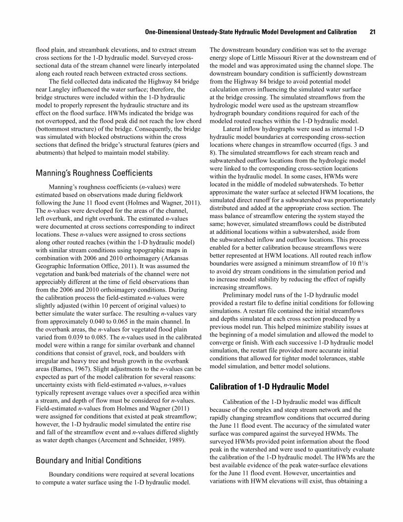
One-Dimensional Unsteady-State Hydraulic Model Development and Calibration 21

flood plain, and streambank elevations, and to extract stream cross sections for the 1-D hydraulic model. Surveyed cross-sectional data of the stream channel were linearly interpolated along each routed reach between extracted cross sections.

The field collected data indicated the Highway 84 bridge near Langley influenced the water surface; therefore, the bridge structures were included within the 1-D hydraulic model to properly represent the hydraulic structure and its effect on the flood surface. HWMs indicated the bridge was not overtopped, and the flood peak did not reach the low chord (bottommost structure) of the bridge. Consequently, the bridge was simulated with blocked obstructions within the cross sections that defined the bridge’s structural features (piers and abutments) that helped to maintain model stability.

Manning’s Roughness CoefficientsManning’s roughness coefficients (n-values) were

estimated based on observations made during fieldwork following the June 11 flood event (Holmes and Wagner, 2011). The n-values were developed for the areas of the channel, left overbank, and right overbank. The estimated n-values were documented at cross sections corresponding to indirect locations. These n-values were assigned to cross sections along other routed reaches (within the 1-D hydraulic model) with similar stream conditions using topographic maps in combination with 2006 and 2010 orthoimagery (Arkansas Geographic Information Office, 2011). It was assumed the vegetation and bank/bed materials of the channel were not appreciably different at the time of field observations than from the 2006 and 2010 orthoimagery conditions. During the calibration process the field-estimated n-values were slightly adjusted (within 10 percent of original values) to better simulate the water surface. The resulting n-values vary from approximately 0.040 to 0.065 in the main channel. In the overbank areas, the n-values for vegetated flood plain varied from 0.039 to 0.085. The n-values used in the calibrated model were within a range for similar overbank and channel conditions that consist of gravel, rock, and boulders with irregular and heavy tree and brush growth in the overbank areas (Barnes, 1967). Slight adjustments to the n-values can be expected as part of the model calibration for several reasons: uncertainty exists with field-estimated n-values, n-values typically represent average values over a specified area within a stream, and depth of flow must be considered for n-values. Field-estimated n-values from Holmes and Wagner (2011) were assigned for conditions that existed at peak streamflow; however, the 1-D hydraulic model simulated the entire rise and fall of the streamflow event and n-values differed slightly as water depth changes (Arcement and Schneider, 1989).

Boundary and Initial ConditionsBoundary conditions were required at several locations

to compute a water surface using the 1-D hydraulic model.

The downstream boundary condition was set to the average energy slope of Little Missouri River at the downstream end of the model and was approximated using the channel slope. The downstream boundary condition is sufficiently downstream from the Highway 84 bridge to avoid potential model calculation errors influencing the simulated water surface at the bridge crossing. The simulated streamflows from the hydrologic model were used as the upstream streamflow hydrograph boundary conditions required for each of the modeled routed reaches within the 1-D hydraulic model.

Lateral inflow hydrographs were used as internal 1-D hydraulic model boundaries at corresponding cross-section locations where changes in streamflow occurred (figs. 3 and 8). The simulated streamflows for each stream reach and subwatershed outflow locations from the hydrologic model were linked to the corresponding cross-section locations within the hydraulic model. In some cases, HWMs were located in the middle of modeled subwatersheds. To better approximate the water surface at selected HWM locations, the simulated direct runoff for a subwatershed was proportionately distributed and added at the appropriate cross section. The mass balance of streamflow entering the system stayed the same; however, simulated streamflows could be distributed at additional locations within a subwatershed, aside from the subwatershed inflow and outflow locations. This process enabled for a better calibration because streamflows were better represented at HWM locations. All routed reach inflow boundaries were assigned a minimum streamflow of 10 ft3/s to avoid dry stream conditions in the simulation period and to increase model stability by reducing the effect of rapidly increasing streamflows.

Preliminary model runs of the 1-D hydraulic model provided a restart file to define initial conditions for following simulations. A restart file contained the initial streamflows and depths simulated at each cross section produced by a previous model run. This helped minimize stability issues at the beginning of a model simulation and allowed the model to converge or finish. With each successive 1-D hydraulic model simulation, the restart file provided more accurate initial conditions that allowed for tighter model tolerances, stable model simulation, and better model solutions.

Calibration of 1-D Hydraulic Model

Calibration of the 1-D hydraulic model was difficult because of the complex and steep stream network and the rapidly changing streamflow conditions that occurred during the June 11 flood event. The accuracy of the simulated water surface was compared against the surveyed HWMs. The surveyed HWMs provided point information about the flood peak in the watershed and were used to quantitatively evaluate the calibration of the 1-D hydraulic model. The HWMs are the best available evidence of the peak water-surface elevations for the June 11 flood event. However, uncertainties and variations with HWM elevations will exist, thus obtaining a


precise match between simulated and measured peak water-surface elevations is often difficult. The simulated water surface produced by a 1-D hydraulic model is flat across all cross sections perpendicular to the main direction of streamflow. In reality, measured HWMs can differ in elevation from the left and right side of a stream. Therefore, several of the 88 collected HWMs located near the same cross-section line were averaged together to represent a single HWM (appendix 1). This resulted in a total of 57 HWMs (primarily near Albert Pike) being used to calibrate the 1-D hydraulic model. For the majority of HWMs (46), a modeled cross section corresponded to the same location, and this allowed for a direct comparison of the HWM elevation with the simulated water-surface elevation. For 11 of the HWMs, their locations were a short distance downstream from a modeled cross section; therefore, a linear interpolation was completed using the simulated water-surface elevations at the upstream and downstream cross sections. On average, the simulated water-surface elevation was interpolated less than 60 ft downstream from an explicitly modeled cross section.

The differences between the measured HWM elevations and simulated peak water-surface elevations were small and indicated a reasonable calibration was achieved with the 1-D hydraulic model. An average error was calculated by subtracting each HWM from the computed water-surface elevation for a selected routed reach, with a negative sign indicating a simulated water-surface elevation above the actual HWM (table 4). The literature for calibrated 1-D hydraulic models shows the difference between measured and simulated data can range from plus or minus 0.0 to more than 1.8 ft (Hunt and others, 1999; Soong and others, 2005; Murphy and others, 2007; Hummel and others, 2012). The average error for the 43 HWMs along the main stem of the Little Missouri River was -0.5 ft, and the overall average for all 57 HWMs was 0.3 ft. Within the area of Albert Pike, a total of 26 HWMs was used to compare the water-surface elevations, the average error was -0.4 ft (reach 2; table 4). Some of the

larger differences occurred at headwater locations, locations where streamflow changed abruptly such as near lateral inflow points (such as tributary inflows), and along parts of a routed reach where supercritical streamflow was likely to have occurred. Supercritical streamflow includes areas of the stream with high velocities and turbulent conditions that can causes sudden and large changes in the water surface making it difficult to simulate with a 1-D hydraulic model. A high degree of confidence can be placed in the 1-D hydraulic model simulation of the water surface for the June 11 flood event because of the inclusion of a relatively high density of HWMs, especially within Albert Pike. In some other cases, the best available data include using 10 or less HWMs to calibrate a stream that is 20 mi or more (Soong and others, 2005; Murphy and others, 2007). In this simulation, the reach of the Little Missouri River that includes Albert Pike is less than 5 mi in total length with 26 HWMs included during calibration.

Simulated Water Depth, Rate of Rise, and Velocities

Peak water-surface elevations, maximum water depths, and peak stream velocities simulated during the flood peak were summarized for cross sections near the approximate location of each indirect (table 5). The simulated water-surface elevation differed by 42.2 ft from upstream to downstream in the 1.5-mi stretch of the Little Missouri River between site 1 and site 4. The peak simulated water-surface elevation for the Little Missouri River changed by 240.7 ft in elevation from the indirect at site 1 to the indirect at site 6 near the Langley streamgage. Among the indirect locations, the maximum simulated water depth of 25.2 with a water-surface elevation of 926.2 ft occurred at site 4 (within Area C campground). The maximum simulated water depths that occurred within Albert Pike were just upstream from site 4 (within the

Table 4. Comparison of surveyed high-water marks and simulated water-surface elevations for the Little Missouri River watershed, Arkansas.

[ft, feet; HWMs, high water marks; difference, surveyed peak water-surface elevation - simulated peak water-surface elevation; ft, feet]

Modeled routed reach (upstream to downstream, see fig. 3)

Average difference

(ft)

Maximum difference

(ft)

Minimum difference

(ft)

Standard deviation

(ft)

Number of HWMs within routed reach

Little Missouri River (routed reach 4) -0.9 0.7 -1.9 0.9 6Long Creek -0.7 1.0 -1.7 1.1 5Little Missouri River (routed reach 3) -0.6 0.4 -1.1 0.7 4Brier Creek 1.7 3.1 0.4 1.1 5Little Missouri River (routed reach 2) -0.4 1.9 -2.5 1.0 26Blaylock Creek -0.4 1.0 -1.7 1.2 4Little Missouri River (routed reach 1) -0.3 0.6 -2.7 1.2 7

Sensitivity Analysis 23

proximity of Area C campground) at 26.8 ft with a water-surface elevation of 930.1 ft. The simulated channel velocity at site 1 increased 3.6 ft/s (from 7.0 ft/s to 10.6 ft/s) along approximately 13 mi of the stream to site 6 at the Langley streamgage. The maximum simulated stream velocity within Albert Pike reached 21.5 ft/s, and occurred just downstream from Area C campground. Among the indirect locations, the highest overbank velocity (10.3 ft/s) occurred on the left overbank at site 4 (within Area C campground). The lowest average simulated velocity for the cross section was 6.6 ft/s and occurred at site 3.

The rapid increase in stage and streamflow that resulted from the June 11 flood event throughout the Little Missouri River watershed is evident by analyzing simulation results at cross-section CS–A (figs. 9 and 10). Cross-section CS-A is located along the Little Missouri River downstream from Brier Creek and the Area D campground, and is an important location to understand the events that occurred within Albert Pike. The water-surface elevations, water depths, stream velocities, and inundated areas were simulated through time for the June 11 flood event. The simulated stage at CS–A began to rise at approximately 1:20 a.m. on June 11 (excluding the initial increase in simulated stage, see “Calibration of Hydrologic Model”). The simulated water surface increased an average of 0.5 ft every 5 minutes for a total of 2 hours, with the maximum rate of rise being 2 ft in 15 minutes. The simulated water surface at CS–A reached a peak elevation of

935 ft with a maximum water depth of 22.2 ft at 4:15 a.m. For comparison, survey data collected at CS–A indicated that water depths of 6 ft or greater are needed to overtop the streambanks, and water depths of approximately 10 ft (measured from the stream channel) are needed to reach the levels of Areas C and D campgrounds.

As the simulated depths increased through time at CS–A, so did the simulated stream velocities. At 10:00 p.m. on June 10, the simulated streamflow in the Little Missouri River was within the channel and had an average velocity of 2.6 ft/s at CS–A. However by 2:00 a.m. on June 11, the average simulated stream velocities in the channel at CS–A increased more than three times to 8.2 ft/s, and the left and right overbank average stream velocities were 4.7 ft/s and 3.4 ft/s, respectively. When the flood peaked at CS–A, near 4:15 a.m., the simulated average velocities in the channel, left overbank, and right overbank were 12.6 ft/s, 9.5 ft/s, and 6.2 ft/s, respectively. The simulated average stream velocity for CS–A at the peak of the flood was 10.0 ft/s.

Sensitivity AnalysisA sensitivity analysis is the determination of the effects

of changes in calibrated model parameters to simulated results. Many simulations were conducted as the models were calibrated, and results from these simulations are the basis

Table 5. Summary of simulated hydraulic properties at the flood peak corresponding to the indirect discharge measurement locations for the Little Missouri River watershed, Arkansas.

[USGS, U.S. Geological Survey; ft/s, feet per second; ft, feet]

Site identifier

(see fig. 1)

Site nameUSGS

station number

Average simulated

velocity for the cross section

(ft/s)

Average simulated velocity in

channel (ft/s)

Average simulated velocity

in left overbank

(ft/s)

Average simulated velocity in right

overbank (ft/s)

Simulated peak

water-surface

elevation (ft)

Simulated maximum

water depth

(ft)

1 Little Missouri River above Long Creek near Albert Pike Recreation Area, Ark.

1073601763 7.0 9.6 9.4 3.6 968.4 19.1

2 Long Creek near Langley, Ark. 107360178 7.6 13.7 4.5 28.6 969.6 14.7

3 Brier Creek near Langley, Ark. 107360183 6.6 8.0 6.8 25.0 985.6 13.4

4 Little Missouri River at Albert Pike Recreation Area, Ark.

107360187 11.5 13.8 10.3 27.7 926.2 25.2

5 Blaylock Creek near Langley, Ark. 107360195 8.8 10.9 3.8 27.0 883.8 11.7

6 Little Missouri River near Langley, Ark.

07360200 10.6 14.5 28.6 9.6 727.7 21.9

1Ungaged location with no continuous streamgage. Site assigned a U.S. Geological Survey station identification number.2Limited overbank area at this location and negligible influence to overall cross-sectional value.

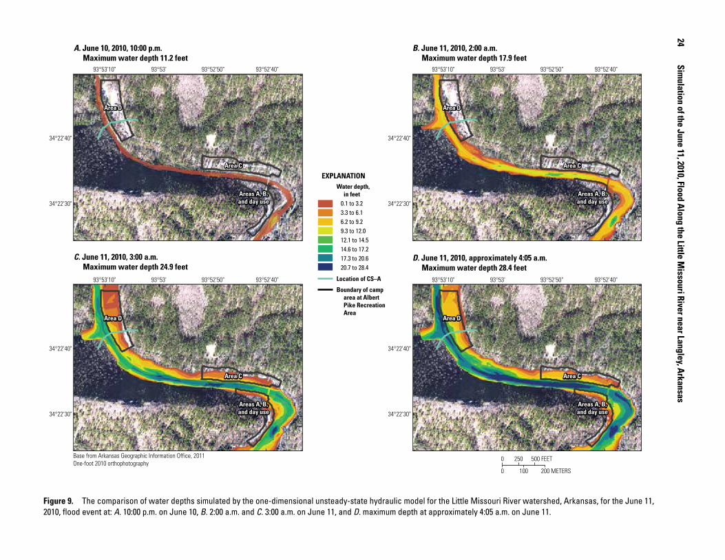
24



Figure 9. The comparison of water depths simulated by the one-dimensional unsteady-state hydraulic model for the Little Missouri River watershed, Arkansas, for the June 11, 2010, flood event at: A. 10:00 p.m. on June 10, B. 2:00 a.m. and C. 3:00 a.m. on June 11, and D. maximum depth at approximately 4:05 a.m. on June 11.

93°52'40"93°52'50"93°53'93°53'10"

34°22'40"

34°22'30"

93°52'40"93°52'50"93°53'93°53'10"

34°22'40"

34°22'30"

93°52'40"93°52'50"93°53'93°53'10"

34°22'40"

34°22'30"

93°52'40"93°52'50"93°53'93°53'10"

34°22'40"

34°22'30"

0 250 500 FEET

0 100 200 METERS

Area D

Area C

Areas A, B,and day use

Area D

Area C


Area D

Area C


Area D

Area C


Area D

Area C


Area D

Area C


Area D

Area C


Area D

Area C


Base from Arkansas Geographic Information Office, 2011One-foot 2010 orthophotography

B. June 11, 2010, 2:00 a.m. Maximum water depth 17.9 feet

A. June 10, 2010, 10:00 p.m. Maximum water depth 11.2 feet

D. June 11, 2010, approximately 4:05 a.m. Maximum water depth 28.4 feet

C. June 11, 2010, 3:00 a.m. Maximum water depth 24.9 feet

EXPLANATIONWater depth, in feet 0.1 to 3.2 3.3 to 6.1 6.2 to 9.2 9.3 to 12.0 12.1 to 14.5 14.6 to 17.2 17.3 to 20.6 20.7 to 28.4

Location of CS–A

Boundary of camp area at Albert Pike Recreation Area

Sensitivity Analysis

25

Figure 10. The comparison of water velocities simulated by the one-dimensional unsteady-state hydraulic model for the Little Missouri watershed, Arkansas, for the June 11, 2010, flood event at: A. 10:00 p.m. on June 10, B. 2:00 a.m. and C. 3:00 a.m. on June 11, and D. maximum velocity at approximately 4:05 a.m. on June 11.

93°52'40"93°52'50"93°53'93°53'10"

34°22'40"

34°22'30"

93°52'40"93°52'50"93°53'93°53'10"

34°22'40"

34°22'30"

93°52'40"93°52'50"93°53'93°53'10"

34°22'40"

34°22'30"

93°52'40"93°52'50"93°53'93°53'10"

34°22'40"

34°22'30"

0 250 500 FEET

0 100 200 METERS

Base from Arkansas Geographic Information Office, 2011One-foot 2010 orthophotography

Area D

Area C


Area D

Area C


Area D

Area C


Area D

Area C


Area D

Area C


Area D

Area C


Area D

Area C


Area D

Area C


D. June 11, 2010, approximately 4:05 a.m. Maximum water velocity 21.5 feet per second

C. June 11, 2010, 3:00 a.m. Maximum water velocity 18.6 feet per second

A. June 10, 2010, 10:00 p.m. Maximum water velocity 4.6 feet per second

B. June 11, 2010, 2:00 a.m. Maximum water velocity 12.0 feet per second

EXPLANATIONWater velocity, in feet per second 0.1 to 1.3 1.4 to 4.0 4.1 to 6.4 6.5 to 8.9 9.0 to 11.4 11.5 to 13.7 13.8 to 16.4 16.5 to 21.5

Location of CS–A

Boundary of camp area at Albert Pike Recreation Area


for the sensitivity analysis. A complete sensitivity analysis for all model parameters was not conducted. The parameters and datasets that had the greatest influence on model results were the precipitation multipliers for the hydrologic model and n-values for the 1-D hydraulic model. Thus, these two parameters were used for the sensitivity analysis.

The hydrologic model was driven by the precipitation data, and model simulations were substantially affected by changes in precipitation intensities and volumes. To test the sensitivity of precipitation intensity, 1-hour and 15-minutes NEXRAD precipitation data were used to drive the hydrologic model. Simulated peak streamflows decreased an average of 17 percent when 1-hour precipitation data were used compared to the simulation that used 15-minute precipitation data. Therefore, the development of 15-minute NEXRAD data was important to the calibration of the hydrologic model to more adequately capture the short duration and high intensity nature of the storm event. Additionally, approximately a 1:1 ratio existed between precipitation multiplier values and the simulated increase in streamflows. A 10-percent increase in precipitation resulted in a 10-percent increase in simulated streamflow.

The most sensitive parameter for the 1-D hydraulic model was identified to be the n-values. A 10-percent increase in calibrated n-values resulted in an average increase of 0.60 ft in the water-surface elevation, and a 10-percent decrease of the n-values resulted in an average decrease of less than 0.1 ft in the water-surface elevation.

Model Limitations and Model Comparison

A model can be used to help understand and solve problems; however, an understanding of model limitations is essential for the effective use and interpretations of model results. The accuracies of both the hydrologic and 1-D hydraulic models are limited by the required simplifications of a complex reality; such as those associated with the mathematical formulation of the governing equations, watershed discretization, spatial and temporal characteristics of precipitation data, and by the availability of appropriate data and the required interpolation and extrapolations that are inherent in using data in any model (Hart and others, 2012). For example, streamflow can be simulated with reasonable accuracy at stream locations with a streamgage; however, at tributaries that do not have streamgages, adequacy of streamflow simulation is uncertain. Although a model might be considered calibrated, calibration parameter values are not unique in yielding acceptable simulated values of streamflows or water-surface elevations.

Both models used in this study had specific limitations relating to the model development and calibration process. Limitations specific to the hydrologic model included the accuracy of NEXRAD data used to provide the input for

the precipitation. The need for multipliers is not unexpected given the uncertainty in the NEXRAD data resulting from the mountainous terrain, range from the radar, sparse precipitation gages, the temporal and spatial scale of the event, and the focus on a relatively small watershed during an extreme single event. The data collected at the Langley streamgage during the June 11 flood event and the indirects and HWMs collected after the flood were imperative in calibrating the model; however, inherent error exists because of the extreme nature of the event. For example, the indirect at the Langley streamgage, which consequently now defines the upper limit of the stage-streamflow relation (rating curve), is approximately four times higher than the next highest measured peak streamflow value (period of record includes 1988 to 2011 [U.S. Geological Survey, 2011b] for peak streamflow data). The resulting rating curve has a large gap in measured streamflows that requires interpolation between values and can introduce uncertainty with peak streamflow measurements. Limitations specific to the 1-D hydraulic model relate to a one-dimensional representation of a three-dimensional water column. In some situations, the one-dimensional assumptions are insufficient to precisely simulate a water-surface elevation. In reality, water surfaces along a cross section are not always flat. A water surface can be superelevated or have different elevations between the inside and outside turns of a stream or be convex or concave along a cross-section line. Possible physical reasons for discrepancies in the simulated water surface include changes in channel geometry between surveyed cross sections, which could not be accounted for by interpolation, errors present within the DEM, and uncertainties associated with the measured data.

The 1-D hydraulic model is limited by a one-dimensional representation of streamflow; therefore, a two-dimensional surface-water model was constructed for the area surrounding Albert Pike (Wagner, 2013). A two-dimensional model can better simulate a water surface, which varies along a cross section, and can simulate stream velocities with less interpolation. Provided that each model simulates a common area with similar boundary conditions, the expectation would be the different models could agree within reason. The mean water depth simulated by the 1-D hydraulic model (for the area in common with the two-dimensional model) was 11.0 ft, and the mean water depth simulated by the two-dimensional model was 10.8 ft. The simulated grids for water depth and stream velocity from each model were directly compared by subtracting the 1-D hydraulic model grid from the two-dimensional model grid. The absolute mean difference for the simulated water depth was 0.9 ft. The mean stream velocity simulated by the 1-D hydraulic model (for the area in common with the two-dimensional model) was 5.7 ft/s, and the mean stream velocity simulated by the two-dimensional model was 6.2 ft/s. The absolute mean difference for the simulated stream velocity was 1.9 ft/s. The results from each model complement the other and increase the understanding of the June 11 flood event.

References Cited 27

SummaryA substantial flood event occurred on June 11, 2010,

causing the Little Missouri River to flow over much of the adjacent land area, resulting in catastrophic damages. Twenty fatalities occurred and numerous automobiles, cabins, and recreational vehicles were destroyed within the U.S. Department of Agriculture—Forest Service (USFS) Albert Pike Recreation Area (Albert Pike), at a dispersed campsite area in the surrounding Ouachita National Forest lands, and at a nearby privately owned camp. The Little Missouri River streamgage near Langley, Arkansas (U.S. Geological Survey station number 07360200), reached a record streamflow of 70,800 cubic feet per second (ft3/s) and a stage (water level) of 23.5 feet (ft) at 5:30 a.m., with a 10-ft rise occurring in slightly more than 1 hour.

To better understand the flood event on June 11, 2010, the U.S. Geological Survey, in cooperation with the USFS, developed a precipitation-runoff hydrologic model, U.S. Army Corps of Engineers Hydrologic Engineering Center Hydrologic Modeling System (HEC–HMS), coupled with a one-dimensional unsteady-state hydraulic model, U.S. Army Corps of Engineers Hydrologic Engineering Center River Analysis System (HEC–RAS), to simulate precipitation runoff and streamflow characteristics along the Little Missouri River and at various tributaries within the 68-square miles watershed upstream from the Langley streamgage. The precipitation input, precipitation excess, base flow, and output hydrograph were estimated using Next-Generation Radar (NEXRAD) precipitation data, initial constant loss model, the recession base-flow method, and the Snyder unit-hydrograph method, respectively, to develop a precipitation-runoff hydrologic model to simulate streamflow change over time. A one-dimensional unsteady-state hydraulic model was used to simulate water-surface elevations, water depths, stream velocities, and areas of inundation.

The hydrologic model was calibrated using indirect discharge measurements and streamgage data. The simulated streamflows compared to the measured streamflows at the Langley streamgage had a coefficient of determination (R2) of 0.98 for the calibration period. Within the proximity of two campgrounds, the Little Missouri River just downstream from the confluence of Brier Creek had a peak simulated streamflow of 49,300 ft3/s at 4:08 a.m., and simulated streamflow stayed within 500 ft3/s of the peak for nearly 15 minutes. Approximately 1.5 hours after the peak streamflow occurred within Albert Pike, the simulated streamflow of 77,600 ft3/s peaked at the Langley streamgage at 5:20 a.m.

The one-dimensional unsteady-state hydraulic model was calibrated using surveyed high-water marks (HWMs). The average error for the 43 HWMs along the main stem of the Little Missouri River was -0.5 ft, and the overall average error for all 57 HWMs was 0.3 ft. The Little Missouri River, just downstream from the confluence of Brier Creek, had a

peak simulated water-surface elevation of 935 ft, a maximum water depth of 22.2 ft, and a maximum stream channel velocity of 12.6 feet per second (ft/s) at 4:15 a.m. Beginning at approximately 1:20 a.m., the simulated water depths for the Little Missouri River just downstream from the confluence of Brier Creek increased an average of 0.5 ft every 5 minutes for a total of 2 hours with the maximum rate of rise being 2 ft in 15 minutes.

The results from the precipitation-runoff hydrologic model, the one-dimensional unsteady-state hydraulic model, and a separate two-dimensional model developed as part of a coincident study each complement the other in terms of streamflow timing, water-surface elevations, and velocities propagated by the June 11, 2010, flood event. The absolute mean difference in water depth simulated by the one-dimensional hydraulic model and two-dimensional model (for the area in common with the two-dimensional model) was 0.9 ft. Additionally, the absolute mean difference in stream velocity simulated by the one-dimensional and two-dimensional models was 1.9 ft/s.

References Cited

Arcement, G.J., Jr., and Schneider, V.R., 1989, Guide for selecting Manning’s roughness coefficients for natural channels and flood plains: U.S. Geological Survey Water Supply Paper 2339, 38 p.

Ahrens, S.R., and Maidment, D.R., 1999, Flood forecasting for the Buffalo Bayou using CRWR–PrePro and HEC–HMS: Austin, Texas, Center for Research in Water Resources Report 99–6, 139 p.

Arkansas Geographic Information Office, 2011, GeoStor, Arkansas’ official GIS platform: Arkansas.gov, accessed January 2011, at http://www.geostor.arkansas.gov/.

Arora K.R., 2004, Irrigation, water power and water resources engineering: New Delhi, Delhi, India, Standard Publishers Distributors, 1705–B, p. 79–106.

Barnes, H.H., Jr., 1967, Roughness characteristics of natural channels: U.S. Geological Survey Water-Supply Paper 1849, 213 p.

Bedient, P.B., Holder, A., Benavide, J., and Vieux, B.E., 2003, Radar-based flood warning system applied to tropical storm Allison: Journal of Hydrologic Engineering, v. 8, no. 6, p. 308–318.

Benson, M.A., and Dalrymple, Tate, 1967, General field and office procedures for indirect discharge measurements: U.S. Geological Survey Techniques of Water-Resources Investigations, book 3, chap. A1, 30 p. (Also available at http://pubs.usgs.gov/twri/twri3-a1/.)

http://www.geostor.arkansas.gov/

http://pubs.usgs.gov/twri/twri3-a1/


Bhunya, P., Panda, S.N., and Goel, M.K., 2011 Synthetic unit hydrograph methods—A critical review: The Open Hydrology Journal, v. 5, no. 1, p. 1–8.

Biggs, E., and Atkinson, P., 2010, A comparison of gauge and radar precipitation data for simulating an extreme hydrological event in the Severn Uplands, UK: Hydrological Processes, v. 25, no. 28, p. 795–810.

Boarh, D.K., 2011, Hydrologic procedures of storm event watershed models—A comprehensive review and comparison: Hydrological Processes, v. 25, no. 22, p. 3472–3489.

Breidenbach, J.P., and Bradberry, J.S., 2001, Multisensor precipitation estimates produced by National Weather Service River Forecast Center for Hydrologic Applications, in 2001 Georgia Water Resources Conference, Proceedings: Institute of Ecology, University of Georgia, Athens, Georgia, p. 1–4.

Chow, V.T., Maidment, D.R., and Mays, L.W., 1988, Applied hydrology: New York, N.Y., McGraw-Hill, 570 p.

Dawdy, D.R., Lichty, R.W., and Bergmann, J.M., 1972, A rainfall-runoff simulation model for estimation of flood peaks for small drainage basins: U.S. Geological Survey Professional Paper 506–B, 27 p.

Department of Commerce Weather Bureau, 1961, Rainfall frequency atlas of the United States: Technical Paper 40, 61 p.

Donigian, A.S., Jr., 2000, HSPF Training Workshop Handbook and CD, Lecture #19—Calibration and Verification Issues, Slide #L19–22: Environmental Protection Agency Headquarters, Washington Information Center, 10–14 January, 2000, Presented and prepared for U.S. Environmental Protection Agency Office of Water, Office of Science and Technology, Washington, D.C.

Dutta, D., Welsh, W., Vaze, J., Kim, S., Nicholls, D., 2012, A comparative evaluation of short-term streamflow forecasting using time series analysis and rainfall-runoff models in eWater source: Water Resources Management, v. 26, no. 15, p. 4397–4415.

El Hassan, A.A, Sharif, H.O., Jackson, Terrance, and Chintalapudi, Singaiah, 2012, Performance of a conceptual and physically based model in simulating the response of a semi-urbanized watershed in San Antonio, Texas: Hydrological Processes, accessed on November 5, 2012, at http://dx.doi.org/10.1002/hyp.9443.

Fulton, R.A., Breidenbach, J.P., Seo, D.J., and Miller, D.A., 1998, The WSR–88D rainfall algorithm: Weather and Forecasting, v. 13, no. 2, p. 377–395.

Grassotti, C., Hoffman, R.N., Vivoni E.R., and Entekhabi, D., 2003, Multiple-timescale intercomparison of two radar products and rain gauge observations over the Arkansas–Red River Basin: Weather and Forecasting, v. 18, no. 6, p. 1207–1229.

Greene, D.G., and Hudlow, M.D., 1982, Hydrometeorologic grid mapping procedures, in Johnson, A.I., and Clark, R.A., American Water Resources Association International Symposium on Hydrometeorology, Proceedings: Denver, Colorado, June 13–17, 1982, 20 p.

Hart, R.M., Green, W.R., Westerman, D.A., Petersen, J.C., and De Lanois, J.L., 2012, Simulated effects of hydrologic, water quality, and land-use changes of the Lake Maumelle watershed, Arkansas, 2004–10: U.S. Geological Survey Scientific Investigations Report 2012–5246, 119 p.

Helsel, D.R., and Hirsch, R.M., 2002, Statistical methods in water resources: U.S. Geological Survey Techniques of Water-Resources Investigation, book 4, chap. A3, 523 p.

Holmes, R.R., Jr., and Wagner, D.M., 2011, Flood of June 11, 2010, in the upper Little Missouri River watershed, Arkansas: U.S. Geological Survey Scientific Investigations Report 2011–5194, 31 p.

Hummel, R., Duan, J.G., and Zhang, S., 2012, Comparison of unsteady and quasi-unsteady flow models in simulating sediment transport in an ephemeral Arizona stream: Journal of the American Water Resources Association, v. 48, no. 5, p. 987–998.

Hunt, J., Brunner, G., and Larock, B., 1999, Flow transitions in bridge backwater analysis: Journal of Hydraulic Engineering, v. 125, no. 9, p. 981–983.

Knebl M.R., Yang, Z.L., Hutchison, K., and Maidment, D.R., 2005, Regional scale flood modeling using NEXRAD rainfall, GIS, and HEC–HMS/RAS: A case study for the San Antonio River Basin summer 2002 storm event: Journal of Environmental Management, v. 75, p. 325–336.

Linsley, R.K., 1986, Flood estimates: How good are they?: Water Resource Research, v. 22, no. 9., p. 159S–164S.

Linsley, R.K., Kohler, M.A., and Paulhus, J.L.H., 1982, Hydrology for engineers: New York, N.Y., McGraw-Hill, 508 p.

Murphy, E.A., Straub, T.D., Soong, D.T., and Hamblen, C.S., 2007, Hydrologic, hydraulic, and flood analyses of the Blackberry Creek watershed, Kendall County, Illinois: U.S. Geological Survey Scientific Investigations Report 2007–5141, 49 p. with appendixes.

National Oceanic and Atmospheric Administration, 2002, About the stage III data: NOAA’s National Weather Service Distributed Model Intercomparison Project, accessed January 26, 2012, at http://www.nws.noaa.gov/oh/hrl/dmip/stageiii_info.htm.

http://dx.doi.org/10.1002/hyp.9443

References Cited 29

National Oceanic and Atmospheric Administration, 2008, Multi-sensor precipitation reanalysis: NOAA National Climatic Data Center, accessed January 26, 2012, at http://www.ncdc.noaa.gov/oa/rsad/mpr.html.

National Oceanic and Atmospheric Administration, 2010a, ABRFC precipitation processing: NOAA National Weather Service River Forecast Center, accessed January 26, 2012, at http://www.srh.noaa.gov/abrfc/?n=pcpn_methods.

National Oceanic and Atmospheric Administration, 2010b, State of the climate national overview June 2010: NOAA National Climatic Data Center, accessed December 20, 2010, at http://www.ncdc.noaa.gov/sotc/national/2010/6.

National Oceanic and Atmospheric Administration, 2011, National Climatic Data Center, accessed July 12, 2011, at http://www.ncdc.noaa.gov.

Ockerman, D.J., and Roussel, M.C., 2009, Simulation of streamflow and water quality in the Leon Creek watershed, Bexar County, Texas, 1997–2004: U.S. Geological Survey Scientific Investigations Report 2009–5191, 50 p.

O’Connor, J.E., and Costa, J.E., 2003, Large floods in the United States—Where they happen and why: U.S. Geological Survey Circular 1245, 13 p.

Olson, J.W., 2007, Soil survey of Montgomery County, Arkansas: U.S. Department of Agriculture, Natural Resources Conservation Services, 613 p.

PRISM Climate Group, 2012, Corvallis, Oregon, Oregon State University, accessed December 20, 2012, at http://prism.oregonstate.edu.

Reed, S.M., and Maidment, D.R., 1995, A GIS procedure for merging NEXRAD precipitation data and digital elevation models to determine rainfall-runoff modeling parameters: Austin, Texas, Center for Research in Water Resources, Report 95–3, 119 p.

Scofield, R.A., and Kuligowski, R.J., 2003, Status and outlook of operational satellite precipitation algorithms for extreme precipitation events: Weather Forecasting, v. 18, p. 1037–1051.

Shedd, R.C., and Fulton, R.A., 1993, WSR–88D Precipitation processing and its use in National Weather Service hydrologic forecasting, in International Symposium on Engineering Hydrology, San Francisco, California, July 25–29, 1993, Proceedings: American Society of Civil Engineers, p. 16–21.

Smith, J.A., Seo, D.J., Baeck, M.L., and Hudlow, M.D., 1996, An intercomparison study of NEXRAD precipitation estimates: Water Resources Research, v. 32, no. 7, p. 2035–2045.

Snyder F.F., 1938, Synthetic unit hydrographs: Transactions of American Geophysical Union v. 19, p. 447–454.

Soong, D.T., Straub, T.D., and Murphy, E.A., 2005, Continuous hydrologic simulation and flood-frequency, hydraulic, and flood-hazard analysis of the Blackberry Creek watershed, Kane County, Illinois: U.S. Geological Survey Scientific Investigations Report 2005–5270, 66 p.

Todini E., 1988, Rainfall-runoff modeling—Past, present and future: Journal of Hydrology, v. 100, p. 341–352.

Upton G.J.G., and Rahimi A.R., 2003, On-line detection of errors in tipping-bucket raingages: Journal of Hydrology, v. 278, p. 197–212.

U.S. Army Corps of Engineers, 1994, Flood-runoff analysis: Engineering Manual 1110–2–1417, 214 p.

U.S. Army Corps of Engineers, Hydrologic Engineering Center, 1996, A pilot application of weather radar-based runoff forecasting Salt River Basin, MO: PR–31, 40 p.

U.S. Army Corps of Engineers, Hydrologic Engineering Center, 1998, HEC–1 Flood hydrograph package user’s manual: Hydrologic Engineering Center, 280 p. with appendixes.

U.S. Army Corps of Engineers, 2000, Hydrologic Engineering Center Hydrologic Modeling System HEC–HMS 3.5 Technical Reference Manual: Hydrologic Engineering Center, 318 p. (Also available at http://www.hec.usace.army.mil/software/hec-hms/documentation/HEC-HMS_Technical%20Reference%20Manual_%28CPD-74B%29.pdf.)

U.S. Army Corps of Engineers, 2010a, Hydrologic Engineering Center Hydrologic Modeling System HEC–HMS 3.5 build 1417: Hydrologic Engineering Center, accessed June 9, 2011, at http://www.hec.usace.army.mil.

U.S. Army Corps of Engineers, 2010b, Hydrologic Engineering Center Hydrologic Modeling System HEC–HMS 3.5 User’s Manual: Hydrologic Engineering Center, 318 p. (Also available at http://www.hec.usace.army.mil/software/hec-hms/documentation/HEC-HMS_Users_Manual_3.5.pdf.)

U.S. Army Corps of Engineers, 2010c, Hydrologic Engineering Center Geospatial Hydrologic Modeling Extension HEC–GeoHMS 5.0: Hydrologic Engineering Center, accessed April 11, 2011, at http://www.hec.usace.army.mil.

U.S. Army Corps of Engineers, 2010d, Hydrologic Engineering Center River Analysis System HEC–RAS 4.1: Hydrologic Engineering Center, accessed November 8, 2010, at http://www.hec.usace.army.mil.

U.S. Army Corps of Engineers, 2010e, HEC–RAS River Analysis System, User’s Manual, Version 4.1: Hydrologic Engineering Center, 790 p. (Also available at http://www.hec.usace.army.mil/software/hec-ras/documents/HEC-RAS_4.1_Users_Manual.pdf.)

http://www.ncdc.noaa.gov/oa/rsad/mpr.html

http://www.ncdc.noaa.gov/sotc/national/2010/6

http://www.ncdc.noaa.gov

http://www.hec.usace.army.mil

http://www.hec.usace.army.mil/software/hec-hms/documentation/HEC-HMS_Users_Manual_3.5.pdf







U.S. Army Corps of Engineers, 2010f, Hydrologic Engineering Center, HEC–GeoRAS GIS tools for support of HEC–RAS using ArcGIS 4.3: Hydrologic Engineering Center, accessed November 8, 2010, at http://www.hec.usace.army.mil.

U.S. Geological Survey, 2010, National hydrography dataset, accessed November 8, 2010, at http://nhd.usgs.gov.

U.S. Geological Survey, 2011a, National elevation dataset, accessed November 8, 2011, at http://ned.usgs.gov.

U.S. Geological Survey, 2011b, USGS water data for the Nation: USGS National Water Information System (NWISWeb), accessed November 8, 2011, at http://waterdata.usgs.gov/nwis.

U.S. Geological Survey, 2012, Indirect measurements of flood of June 11, 2010 in the upper Little Missouri watershed, Arkansas: USGS Surface Water Information, accessed, March 6, 2012, at http://water.usgs.gov/floods/reports/LittleMOJune2010/Indirects/.

Wagner, D.M., 2013, Two-dimensional simulation of the June 11, 2010, flood of the Little Missouri River at Albert Pike Recreation Area, Ouachita National Forest, Arkansas: U.S. Geological Survey Scientific Investigations Report 2012–5274, 28 p.

White, G.F., 1945, Human adjustments to floods: Chicago, University of Chicago Press, 225 p.

Williams, L.R., Taylor, C.M., Warren, M.L., Jr., and Clingenpeel, J.A., 2003, Environmental variability, historical contingency, and the structure of regional fish and macroinvertebrate faunas in Ouachita Mountain stream systems: Environmental Biology of Fishes, v. 67, p. 203–216.

Xu, Z., Godrej, A.N., and Grizzard, T.J., 2007, The hydrological calibration and validation of a complexly-linked watershed-reservoir model for the Occoquan watershed, Virginia: Journal of Hydrology, v. 345, p. 167–183.



http://nhs.usgs.gov

http://ned.usgs.gov

Appendix 1—High-Water Marks Used to Calibrate the One-Dimensional Hydraulic Model of the Little Missouri River Watershed, Arkansas

Appendix 1 33

Appendix 1. High-water marks used to calibrate the one-dimensional hydraulic model of the Little Missouri River watershed, Arkansas.—Continued

[NAVD 88, North American Vertical Datum of 1988; NA, not applicable; Quality rating of the high-water mark from Benson and Dalrymple, 1967]

High-water mark number1

Elevation (feet above NAVD 88)

Longitude Latitude River Reach Quality

1A 1,136.77 93°55′8.13″ 34°25′7.42″ Little Missouri River 4 Good2A 1,135.25 93°55′7.16″ 34°25′7.30″ Little Missouri River 4 Good3 1,048.49 93°54′18.93″ 34°24′25.39″ Little Missouri River 4 Good4 967.63 93°52′45.99″ 34°23′21.38″ Little Missouri River 4 Good5 967.49 93°52′46.37″ 34°23′20.83″ Little Missouri River 4 Good6 966.60 93°52′46.49″ 34°23′19.08″ Little Missouri River 4 Good7 959.56 93°52′43.45″ 34°23′13.48″ Little Missouri River 4 Poor8B 1,086.15 93°55′54.18″ 34°23′38.30″ Long Creek 1 Fair9B 1,086.14 93°55′54.60″ 34°23′37.88″ Long Creek 1 Poor

10B 1,084.52 93°55′54.25″ 34°23′39.48″ Long Creek 1 Good11B 1,084.37 93°55′54.11″ 34°23′39.52″ Long Creek 1 Fair12C 1,021.11 93°54′26.67″ 34°23′44.04″ Long Creek 1 Good13C 1,020.66 93°54′27.81″ 34°23′44.24″ Long Creek 1 Good14D 968.41 93°53′41.79″ 34°23′19.11″ Long Creek 1 Good15D 968.01 93°53′41.45″ 34°23′18.47″ Long Creek 1 Fair16 965.89 93°53′39.78″ 34°23′16.91″ Long Creek 1 Good17E 964.61 93°53′37.89″ 34°23′15.42″ Long Creek 1 Good18E 963.79 93°53′36.22″ 34°23′14.91″ Long Creek 1 Good19E 963.70 93°53′38.54″ 34°23′13.58″ Long Creek 1 Poor20F 937.87 93°53′11.99″ 34°22′45.83″ Little Missouri River 3 Poor21F 937.75 93°53′7.62″ 34°22′46.47″ Little Missouri River 3 NA22 936.50 93°53′7.62″ 34°22′45.39″ Little Missouri River 3 Excellent23 936.19 93°53′7.54″ 34°22′44.76″ Little Missouri River 3 Excellent24G 936.02 93°53′7.82″ 34°22′44.40″ Little Missouri River 3 Excellent25G 935.98 93°53′7.78″ 34°22′44.40″ Little Missouri River 3 Excellent26H 1,119.46 93°55′17.03″ 34°23′1.02″ Brier Creek 1 Fair27H 1,118.68 93°55′16.71″ 34°23′0.36″ Brier Creek 1 Fair28I 1,031.32 93°54′19.68″ 34°22′58.83″ Brier Creek 1 Fair29I 1,030.87 93°54′19.74″ 34°22′58.03″ Brier Creek 1 Good30 985.94 93°53′52.70″ 34°22′51.11″ Brier Creek 1 Good31 984.09 93°53′50.32″ 34°22′50.50″ Brier Creek 1 Fair32J 981.96 93°53′48.92″ 34°22′49.96″ Brier Creek 1 Poor33J 981.66 93°53′48.82″ 34°22′49.90″ Brier Creek 1 Poor34 934.54 93°53′4.82″ 34°22′41.55″ Little Missouri River 2 Fair35 934.22 93°53′4.71″ 34°22′41.03″ Little Missouri River 2 Fair36 931.07 93°53′3.38″ 34°22′39.67″ Little Missouri River 2 Poor37 928.98 93°53′0.32″ 34°22′38.49″ Little Missouri River 2 Poor38K 927.21 93°52′57.80″ 34°22′37.67″ Little Missouri River 2 Fair39K 926.98 93°52′57.78″ 34°22′37.62″ Little Missouri River 2 Fair40L 926.29 93°52′52.78″ 34°22′34.14″ Little Missouri River 2 Excellent41L 925.54 93°52′52.60″ 34°22′37.36″ Little Missouri River 2 Fair42L 925.36 93°52′52.64″ 34°22′37.30″ Little Missouri River 2 Fair43L 925.15 93°52′52.66″ 34°22′37.27″ Little Missouri River 2 Fair44M 925.03 93°52′49.96″ 34°22′37.00″ Little Missouri River 2 Fair45 924.68 93°52′51.50″ 34°22′34.09″ Little Missouri River 2 NA

Appendix 1. High-water marks used to calibrate the one-dimensional hydraulic model of the Little Missouri River watershed, Arkansas.


Appendix 1


Appendix 1. High-water marks used to calibrate the one-dimensional hydraulic model of the Little Missouri River watershed, Arkansas.—Continued


High-water mark number1

Elevation (feet above NAVD 88)

Longitude Latitude River Reach Quality

46N 924.58 93°52′51.79″ 34°22′37.14″ Little Missouri River 2 Excellent47N 924.42 93°52′51.84″ 34°22′37.07″ Little Missouri River 2 Excellent48M 924.37 93°52′49.50″ 34°22′37.10″ Little Missouri River 2 Poor49O 924.02 93°52′49.03″ 34°22′34.04″ Little Missouri River 2 Poor50M 923.56 93°52′49.83″ 34°22′34.08″ Little Missouri River 2 Fair51O 923.32 93°52′49.01″ 34°22′34.04″ Little Missouri River 2 Fair52 922.93 93°52′46.91″ 34°22′33.75″ Little Missouri River 2 Fair53P 922.65 93°52′45.09″ 34°22′33.60″ Little Missouri River 2 Good54P 922.30 93°52′45.17″ 34°22′33.50″ Little Missouri River 2 Excellent55 920.61 93°52′37.36″ 34°22′34.55″ Little Missouri River 2 Poor56 919.78 93°52′41.02″ 34°22′32.66″ Little Missouri River 2 Fair57Q 916.61 93°52′39.48″ 34°22′30.12″ Little Missouri River 2 Poor58Q 915.99 93°52′40.13″ 34°22′30.08″ Little Missouri River 2 Poor59R 915.35 93°52′36.91″ 34°22′28.21″ Little Missouri River 2 NA60R 913.28 93°52′39.76″ 34°22′29.17″ Little Missouri River 2 NA61S 912.66 93°52′46.35″ 34°22′23.22″ Little Missouri River 2 Excellent62 912.57 93°52′43.24″ 34°22′25.47″ Little Missouri River 2 Excellent63 912.14 93°52′45.44″ 34°22′24.62″ Little Missouri River 2 Good64S 911.85 93°52′45.15″ 34°22′22.86″ Little Missouri River 2 Good65 911.40 93°52′47.54″ 34°22′19.38″ Little Missouri River 2 Good66 910.81 93°52′46.61″ 34°22′16.47″ Little Missouri River 2 Poor67T 910.30 93°52′46.57″ 34°22′15.20″ Little Missouri River 2 Good68T 910.28 93°52′46.59″ 34°22′15.28″ Little Missouri River 2 Fair69 910.27 93°52′48.38″ 34°22′13.43″ Little Missouri River 2 Poor70 910.19 93°52′46.82″ 34°22′15.99″ Little Missouri River 2 Excellent71 907.07 93°52′48.33″ 34°22′2.69″ Little Missouri River 2 Good72 904.98 93°52′41.79″ 34°22′0.01″ Little Missouri River 2 Good73 884.76 93°54′26.18″ 34°22′5.03″ Blaylock Creek 1 Fair74 880.04 93°54′22.46″ 34°22′3.33″ Blaylock Creek 1 Good75 874.66 93°54′18.35″ 34°21′59.14″ Blaylock Creek 1 Good76U 874.42 93°54′17.31″ 34°21′58.07″ Blaylock Creek 1 Fair77U 873.78 93°54′15.77″ 34°21′59.8″ Blaylock Creek 1 Poor78 818.76 93°54′41.85″ 34°20′59.12″ Little Missouri River 1 Good79V 789.04 93°55′1.32″ 34°20′29.03″ Little Missouri River 1 Fair80V 787.96 93°55′4.94″ 34°20′28.82″ Little Missouri River 1 Poor81W 772.75 93°54′42.75″ 34°19′51.88″ Little Missouri River 1 Good82W 772.52 93°54′45.71″ 34°19′50.82″ Little Missouri River 1 Good83W 772.47 93°54′45.46″ 34°19′50.96″ Little Missouri River 1 Good84 741.58 93°54′29.48″ 34°19′8.52″ Little Missouri River 1 Good85 728.79 93°53′57.71″ 34°18′42.65″ Little Missouri River 1 Poor86 728.23 93°54′1.62″ 34°18′40.33″ Little Missouri River 1 Good87X 711.02 93°53′10.62″ 34°18′4.70″ Little Missouri River 1 Good88X 710.15 93°53′8.46″ 34°18′9.28″ Little Missouri River 1 Poor

1High-water mark numbers with matching superscript letters were averaged together.

Publishing support provided byLafayette Publishing Service Center

Westerm

an and Clark—Sim

ulation of the June 11, 2010, Flood Along the Little M

issouri River near Langley, Arkansas—

SIR 2013–5056

simulation of the june 11, 2010, flood along the little missouri … · front cover, downstream...

Documents