simultaneous plant/controller optimization of traction
TRANSCRIPT
Simultaneous Plant/Controller Optimization of
Traction Control for Electric Vehicle
by
Kuo-Feng Tong
A thesis
presented to the University of Waterloo
in fulfilment of the
thesis requirement for the degree of
Master of Applied Science
in
Electrical and Computer Engineering
Waterloo, Ontario, Canada, 2007
c© Kuo-Feng Tong 2007


I hereby declare that I am the sole author of this thesis. This is a true copy of the
thesis, including any required final revisions, as accepted by my examiners.
I understand that my thesis may be made electronically available to the public.
iii

Abstract
Development of electric vehicles is motivated by global concerns over the need
for environmental protection. In addition to its zero-emission characteristics, an
electric propulsion system enables high performance torque control that may be
used to maximize vehicle performance obtained from energy-efficient, low rolling
resistance tires typically associated with degraded road-holding ability.
A simultaneous plant/controller optimization is performed on an electric vehicle
traction control system with respect to conflicting energy use and performance
objectives. Due to system nonlinearities, an iterative simulation-based optimization
approach is proposed using a system model and a genetic algorithm (GA) to guide
search space exploration.
The system model consists of: a drive cycle with a constant driver torque request
and a step change in coefficient of friction, a single-wheel longitudinal vehicle model,
a tire model described using the Magic Formula and a constant rolling resistance,
and an adhesion gradient fuzzy logic traction controller.
Optimization is defined in terms of the all at once variable selection of: either
a performance oriented or low rolling resistance tire, the shape of a fuzzy logic
controller membership function, and a set of fuzzy logic controller rule base conclu-
sions. A mixed encoding, multi-chromosomal GA is implemented to represent the
variables, respectively, as a binary string, a real-valued number, and a novel rule
base encoding based on the definition of a partially ordered set (poset) by delta
inclusion.
Simultaneous optimization results indicate that, under straight-line acceleration
and unless energy concerns are completely neglected, low rolling resistance tires
should be incorporated in a traction control system design since the energy saving
benefits outweigh the associated degradation in road-holding ability. The results
also indicate that the proposed novel encoding enables the efficient representation
of a fix-sized fuzzy logic rule base within a GA.
iv

Acknowledgments
I would like to thank my two supervisors Professor David W.L. Wang and
Professor Robert B. Gorbet for their vision, guidance, and consultation.
I would like to thank my readers Professor Mehrdad Kazerani and Professor
John McPhee for providing valuable feedback on this work.
I would like to thank the Natural Sciences and Engineering Research Council
of Canada (NSERC), and Earl Hughson, President of Solectron Invotronics, for
supporting my studies through the Industrial Postgraduate Scholarship program.
I would like to thank Thomas Frommer, Yarko Matkiwsky, and the rest of
the Research and Development team at Solectron Invotronics for a delightful and
educational industrial work experience as part of their team.
I would like to thank the many sponsors and organizers of the Challenge X
vehicle design competition and, in particular, the University of Waterloo Alternative
Fuels Team (UWAFT) for the hands-on experience in developing an advanced fuel
cell electric vehicle.
This work was made possible by the facilities of the Shared Hierarchical Aca-
demic Research Computing Network (SHARCNET:www.sharcnet.ca).
I would like to thank my parents and brothers for their continued love and
support.
v


Contents
1 Introduction 1
1.1 Research Objectives and Contributions . . . . . . . . . . . . . . . . 5
1.2 Overview . . . . . . . . . . . . . . . . . . . . . . . . . . . . . . . . . 5
2 Plant Modeling 9
2.1 Case Study Drive Cycle . . . . . . . . . . . . . . . . . . . . . . . . 9
2.2 Vehicle Dynamics . . . . . . . . . . . . . . . . . . . . . . . . . . . . 10
2.2.1 Assumptions . . . . . . . . . . . . . . . . . . . . . . . . . . . 10
2.2.2 Single-Wheel Longitudinal Model . . . . . . . . . . . . . . . 12
2.2.3 Measuring Energy Use and Performance . . . . . . . . . . . 14
2.3 Tire Model . . . . . . . . . . . . . . . . . . . . . . . . . . . . . . . 15
2.3.1 Longitudinal Tire Force Generation . . . . . . . . . . . . . . 15
2.3.2 Rolling Resistance . . . . . . . . . . . . . . . . . . . . . . . 23
2.3.3 Performance versus Energy Efficient Tire . . . . . . . . . . . 26
2.4 Plant Model Summary . . . . . . . . . . . . . . . . . . . . . . . . . 29
3 Control 31
3.1 Traction Control Systems . . . . . . . . . . . . . . . . . . . . . . . 31
3.2 Fuzzy Logic Control . . . . . . . . . . . . . . . . . . . . . . . . . . 36
3.2.1 Fuzzy Sets . . . . . . . . . . . . . . . . . . . . . . . . . . . . 36
3.2.2 Properties of Membership Functions . . . . . . . . . . . . . 38
3.2.3 Controller Input and Output Space . . . . . . . . . . . . . . 42
3.2.4 Fuzzification . . . . . . . . . . . . . . . . . . . . . . . . . . . 43
vii

3.2.5 Inferencing . . . . . . . . . . . . . . . . . . . . . . . . . . . 44
3.2.6 Defuzzification . . . . . . . . . . . . . . . . . . . . . . . . . 47
3.2.7 Research in Fuzzy Logic Control . . . . . . . . . . . . . . . . 51
3.3 Adhesion Gradient Traction Controller . . . . . . . . . . . . . . . . 53
3.3.1 Controller Inputs and Output . . . . . . . . . . . . . . . . . 53
3.3.2 Membership Functions . . . . . . . . . . . . . . . . . . . . . 54
3.3.3 Rule Base . . . . . . . . . . . . . . . . . . . . . . . . . . . . 55
4 Optimization Problem Formulation and Solution Strategy 59
4.1 Simultaneous Plant/Controller Optimization . . . . . . . . . . . . . 59
4.1.1 Plant/Controller Coupling . . . . . . . . . . . . . . . . . . . 60
4.1.2 Optimization Strategies . . . . . . . . . . . . . . . . . . . . 62
4.2 Problem Formulation . . . . . . . . . . . . . . . . . . . . . . . . . . 64
4.2.1 Combined Plant and Controller System . . . . . . . . . . . . 64
4.2.2 Decision Variables and Constraints . . . . . . . . . . . . . . 65
4.2.3 Objective Function . . . . . . . . . . . . . . . . . . . . . . . 67
4.2.4 Problem Summary . . . . . . . . . . . . . . . . . . . . . . . 69
4.3 Solution Strategy . . . . . . . . . . . . . . . . . . . . . . . . . . . . 70
4.3.1 All At Once Variable Selection . . . . . . . . . . . . . . . . . 70
4.3.2 Simulation Optimization . . . . . . . . . . . . . . . . . . . . 72
5 Genetic Algorithm Design 75
5.1 Genetic Algorithms . . . . . . . . . . . . . . . . . . . . . . . . . . . 75
5.1.1 Unconstrained Binary GA . . . . . . . . . . . . . . . . . . . 76
5.1.2 Mixed Encodings and Multi-Chromosomal GA . . . . . . . . 83
5.1.3 Constraint Handling . . . . . . . . . . . . . . . . . . . . . . 87
5.1.4 Parallel Architecture . . . . . . . . . . . . . . . . . . . . . . 92
5.1.5 Genetic-Fuzzy Control . . . . . . . . . . . . . . . . . . . . . 93
5.2 GA in Traction Control System Optimization . . . . . . . . . . . . 96
5.2.1 Decision Variable Encoding . . . . . . . . . . . . . . . . . . 97
5.2.2 Fitness Evaluation and Selection . . . . . . . . . . . . . . . 99
5.2.3 Chromosome Shuffling and Crossover . . . . . . . . . . . . . 100
viii
5.2.4 Multi-Chromosomal Mutation . . . . . . . . . . . . . . . . . 101
5.3 Novel Fuzzy Logic Rule Base Encoding . . . . . . . . . . . . . . . . 102
5.3.1 Set Theory . . . . . . . . . . . . . . . . . . . . . . . . . . . 104
5.3.2 Novel Partial Ordering by Delta Inclusion . . . . . . . . . . 109
5.3.3 Application to Rule Base Encoding . . . . . . . . . . . . . . 114
6 Numerical Results 125
6.1 Numerical Solver Settings . . . . . . . . . . . . . . . . . . . . . . . 125
6.2 Open Loop System Evaluation . . . . . . . . . . . . . . . . . . . . . 126
6.2.1 Open Loop Instability of nTCSu . . . . . . . . . . . . . . . 127
6.2.2 Limited-Torque Open Loop Control of nTCSs . . . . . . . . 131
6.3 Closed Loop System Evaluation . . . . . . . . . . . . . . . . . . . . 134
6.3.1 Closed Loop Response of TCSo . . . . . . . . . . . . . . . . 135
6.3.2 Comparison with Open Loop Systems . . . . . . . . . . . . . 139
6.3.3 Parametric Study on Performance and Energy Use . . . . . 142
6.4 Simultaneous Optimization Results . . . . . . . . . . . . . . . . . . 151
6.4.1 GA Parameters . . . . . . . . . . . . . . . . . . . . . . . . . 151
6.4.2 Impact of Energy Use to Performance Weighting . . . . . . . 152
6.4.3 Evolutionary Performance of the GA . . . . . . . . . . . . . 158
7 Conclusions and Future Work 165
7.1 Future Work . . . . . . . . . . . . . . . . . . . . . . . . . . . . . . . 169
A Traction Control System Parameters 175
B Longitudinal Bicycle Model 179
C Tire Operating Conditions 183
D Simulation Convergence Data 187
E Steady State and Limit Condition Calculations 189
ix


List of Figures
1.1 Major EV Subsystems . . . . . . . . . . . . . . . . . . . . . . . . . 2
1.2 Plant/Controller Design Coupling . . . . . . . . . . . . . . . . . . . 4
2.1 Case Study Drive Cycle . . . . . . . . . . . . . . . . . . . . . . . . 10
2.2 Vehicle Six Primary Degrees of Freedom . . . . . . . . . . . . . . . 11
2.3 Longitudinal Single-Wheel Model . . . . . . . . . . . . . . . . . . . 12
2.4 Velocity of Slip Points S (Driven) and S’ (Free Rolling) . . . . . . . 17
2.5 Longitudinal Tire Force Characteristic . . . . . . . . . . . . . . . . 19
2.6 Energy Flow for a Typical ICE Midsize Passenger Car . . . . . . . 24
2.7 Speed, Pressure, and Loading vs Rolling Resistance . . . . . . . . . 25
2.8 Speed and Temperature vs Rolling Resistance . . . . . . . . . . . . 26
2.9 Longitudinal Force and Force Derivative . . . . . . . . . . . . . . . 28
2.10 Driving Friction Coefficient and Adhesion Gradient . . . . . . . . . 28
3.1 General Structure of a Traction Control System . . . . . . . . . . . 32
3.2 Driving Friction Coefficient . . . . . . . . . . . . . . . . . . . . . . 33
3.3 Fuzzy Logic Control System . . . . . . . . . . . . . . . . . . . . . . 37
3.4 Comparison of a) Crisp Set Boundary and b) Fuzzy Set Boundary . 38
3.5 Core, Support, and Boundaries of a Fuzzy Set . . . . . . . . . . . . 39
3.6 Membership Functions: a) Triangular, and b) Single-Point . . . . . 41
3.7 Membership in Multiple Fuzzy Sets . . . . . . . . . . . . . . . . . . 41
3.8 Fuzzy Set a) Union, b) Intersection, c) Complement . . . . . . . . . 42
3.9 Division of Universe Xi into Triangular Fuzzy Sets . . . . . . . . . . 44
3.10 Double-Input, Single-Output FAM Table . . . . . . . . . . . . . . . 47
xi

3.11 Fuzzy Inference Diagram . . . . . . . . . . . . . . . . . . . . . . . . 50
3.12 Torque Request Input Membership Functions . . . . . . . . . . . . 57
3.13 Adhesion Gradient Input Membership Functions . . . . . . . . . . . 57
3.14 Torque Output Membership Function . . . . . . . . . . . . . . . . . 57
3.15 Rule Base a) Original Rules, and b) Rules for Optimization . . . . . 57
3.16 Fuzzy Logic Traction Controller Surface Plot . . . . . . . . . . . . . 58
4.1 Plant/Controller Optimization and Coupling Loop . . . . . . . . . . 62
4.2 Plant/Controller Optimization Strategies . . . . . . . . . . . . . . . 63
4.3 Traction Control System Model . . . . . . . . . . . . . . . . . . . . 65
4.4 Traction Control Optimization Variables and Objective Function . . 71
4.5 Simulation Optimization Model . . . . . . . . . . . . . . . . . . . . 72
4.6 Optimization Loop Using Traction Control Simulation Model . . . . 73
5.1 Genetic Algorithm Structure . . . . . . . . . . . . . . . . . . . . . . 76
5.2 Genes, Chromosomes, and Population . . . . . . . . . . . . . . . . . 77
5.3 Roulette Wheel Selection a) Direct Mapping, b) Ranking Scheme . 80
5.4 Example of One-Point Crossover . . . . . . . . . . . . . . . . . . . . 82
5.5 Example of Bit Mutation . . . . . . . . . . . . . . . . . . . . . . . . 82
5.6 Effect of Crossover in a) Binary GA and b) Integer GA . . . . . . . 84
5.7 Candidate Solution Representation in Multi-Chromosomal GA . . . 86
5.8 Chromosome Shuffling and Crossover . . . . . . . . . . . . . . . . . 87
5.9 Search Space with Feasible and Infeasible Parts . . . . . . . . . . . 89
5.10 Global GA . . . . . . . . . . . . . . . . . . . . . . . . . . . . . . . . 93
5.11 Rule Base Optimization Variables . . . . . . . . . . . . . . . . . . . 95
5.12 GA for Membership Function & Rule Base Optimization . . . . . . 96
5.13 Structure of Mixed Encoding, Multi-Chromosomal GA . . . . . . . 97
5.14 Encoding of Traction Control System Design Variables . . . . . . . 98
5.15 Random Chromosome Shuffle or Crossover Operation . . . . . . . . 101
5.16 Multi-Chromosomal Mutation . . . . . . . . . . . . . . . . . . . . . 102
5.17 Example Hasse Diagram of a Partially Ordered Set by Inclusion . . 108
5.18 Hasse Diagram of Poset by Delta Inclusion with Level Indications . 112
xii

5.19 Poset by Delta Inclusion of Traction Control Rule Base . . . . . . . 117
5.20 Example of Traction Control Rule Base Crossover by Meet . . . . . 121
5.21 Example of Traction Control Rule Base Crossover by Join . . . . . 122
5.22 Example of Traction Control Rule Base Mutation . . . . . . . . . . 123
6.1 Unstable Open Loop System Response of nTCSu . . . . . . . . . . 128
6.2 Tire and Vehicle Dynamics . . . . . . . . . . . . . . . . . . . . . . . 129
6.3 Marginally Stable Open Loop System Response of nTCSs . . . . . . 133
6.4 Closed Loop Traction Control System Dynamics . . . . . . . . . . . 135
6.5 Closed Loop Fuzzy Logic Traction Control (Nominal Parameters) . 137
6.6 Surface Plot Trajectory of TCSo . . . . . . . . . . . . . . . . . . . . 138
6.7 Closed Loop Traction Control vs Open Loop Control . . . . . . . . 140
6.8 Electric Propulsion System Power Flow . . . . . . . . . . . . . . . . 143
6.9 Parametric Impact on Performance and Energy . . . . . . . . . . . 146
6.10 Parametric Variation in Fuzzy Logic Controller . . . . . . . . . . . 148
6.11 A-PS Variation in Traction Controller Rule Base of TCS1 . . . . . . 156
6.12 Approximation of Pareto Set . . . . . . . . . . . . . . . . . . . . . . 159
6.13 Evolutionary Performance of the GA for TCS4 . . . . . . . . . . . . 160
6.14 Optimization Variable Distribution for TCS4 . . . . . . . . . . . . . 162
B.1 Longitudinal Bicycle Model During Braking . . . . . . . . . . . . . 179
C.1 Position, Motion, Forces, and Moments for Road and Tire . . . . . 184
xiii


List of Tables
1.1 Examples of Potential Vehicle Optimization Variables . . . . . . . . 4
2.1 Approaches to Tire Modeling . . . . . . . . . . . . . . . . . . . . . 16
3.1 Traction Control Strategies . . . . . . . . . . . . . . . . . . . . . . . 35
5.1 Example Roulette Wheel Selection on Minimization Problem . . . . 81
5.2 Preliminary Set Theory Notation . . . . . . . . . . . . . . . . . . . 104
6.1 Open Loop System Configurations . . . . . . . . . . . . . . . . . . . 127
6.2 Steady State and Limit Conditions of nTCSu . . . . . . . . . . . . 130
6.3 Closed Loop Traction Control System Configurations . . . . . . . . 135
6.4 Closed Loop vs Open Loop Performance and Energy Use . . . . . . 142
6.5 Impact of System Design on Performance and Energy Use . . . . . 145
6.6 Percentage of Energy Stored in Vehicle Kinetic Energy . . . . . . . 150
6.7 GA Parameters . . . . . . . . . . . . . . . . . . . . . . . . . . . . . 151
6.8 Optimization Results for Various Energy Weights wE . . . . . . . . 153
6.9 Impact of A-PS Variation in TCS1 on Objectives . . . . . . . . . . 155
6.10 Improvement in Optimized Systems over Benchmark TCSo . . . . . 157
A.1 Single-Wheel Vehicle Parameters . . . . . . . . . . . . . . . . . . . 175
A.2 Drive Cycle Parameters . . . . . . . . . . . . . . . . . . . . . . . . 176
A.3 Tire Parameters . . . . . . . . . . . . . . . . . . . . . . . . . . . . . 176
A.4 Fuzzy Logic Controller Parameters . . . . . . . . . . . . . . . . . . 177
C.1 Tire Operating Modes . . . . . . . . . . . . . . . . . . . . . . . . . 185
xv

D.1 Numerical Solver Convergence Data . . . . . . . . . . . . . . . . . . 188
xvi

Chapter 1
Introduction
Global concerns over climate change have created the need for environmental pro-
tection and action in sustainable development. Temperature rises within the past
35-50 years are attributed to anthropogenic (human) activity causing an increase in
green house gas (GHG) concentration within the atmosphere with CO2 emissions
contributing to the majority (60%) of observed changes [1]. Measurements of world-
wide GHG emissions indicate that the transportation sector is responsible for 21%
of CO2 emissions [2]. Within the transportation sector, CO2 emissions can be ac-
counted for by a strong dependence (94.4%) on non-renewable petroleum products
[3] with primary energy use (73%) in land vehicles [4]. Combined with a projected
47% increase in world oil consumption from 2003 to 2030, with transportation ac-
counting for approximately half the total [5], it is clear that development of low
emission, energy efficient automotive technology is key to mitigating adverse effects
of global warming [1]. From this standpoint, the conventional petroleum-based in-
ternal combustion engine (ICE) is non-ideal due to the release of GHG trapped
within fossil fuels, and a narrow range of optimal operating efficiency [6]. Although
innovations in adapting ICE technology to alternative and renewable fuels [7] have
been partially successful in curbing emissions and attaining higher levels of fuel
economy, further reductions and efficiency improvements are possible in an electric
vehicle (EV) where an electric propulsion system is used either in conjunction with,
or in place of, an ICE [8].
1

Electric Propulsion Subsystem
- Energy Source
- Refuelling Unit
- Power Steering
- Temperature Control
Electronic
Controller
Power
Converter
Electric
Motor
Mechanical
Transmission
Wheel
Wheel
Brake
Accelerate
SteeringEnergy Source Subsystem Auxiliary Subsystem
Figure 1.1: Major EV Subsystems [9]
As shown in Figure 1.1, the electric propulsion system is the core component
of an electric vehicle (EV). Regardless of the electrical energy source, which may
be provided by batteries, a fuel cell, or an ICE-powered generator, an EV relies
on electronic control of a power converter and electric motor to efficiently deliver
power to the wheels. Characteristics of an electric propulsion system include a
high operating efficiency over a wide range of speed and torque demands, energy
recovery during regenerative braking (assuming a power receptive energy source),
and quick, accurate, torque response [9] [10].
Though high efficiency operation and regenerative braking directly benefit fuel
economy, recent research has suggested that further energy savings may be obtained
by the use of high performance traction control and energy efficient, low rolling
resistance tires [11] [12]. Such a control system relies on the fast torque response of
an electric propulsion system to compensate for degraded road adhesion associated
with low rolling resistance tires [12]. Existing research has produced controllers
that enable tire operation near the limits of performance [11] [12] [13]. However, the
trade-offs between vehicle performance and energy economy resulting from the use
of low rolling resistance tires with appropriate control has yet to be addressed. Since
tire selection and controller tuning (plant and controller variables, respectively)
both influence system level objectives in performance and energy consumption, the
problem of balancing these high-level vehicle design requirements can be classified
2

as a multi-objective, simultaneous optimization problem of plant and controller
variables.
In automotive powertrain designs, a sequential plant then controller design pro-
cess is typically taken to manage the complexity associated with each process.
However, it has been recognized that the sequential powertrain design approach
may not allow full optimization of the overall plant/controller system [14]. Si-
multaneous consideration of a combined plant/controller design problem enables
further optimization with respect to system level design objectives. For example,
the optimization of powertrain components selection with respect to cost [15] may
be considered a separate problem from tuning a powertrain control strategy for op-
timal efficiency [16]. The final design may be non-optimal since the electric motor
may be over-sized with respect to utilization by the control strategy. Thus inde-
pendent optimization of component selection and control strategy may result in
higher cost associated with an oversized motor as well as an unnecessary increase
in vehicle mass.
Although simultaneous plant/controller optimization offers potential to improve
overall system design, its application to large scale problems is limited by the in-
creased complexity of the associated optimization problem and available solution
techniques. In general, a simultaneous optimization must consider a “coupling
loop” between plant and controller designs that is illustrated in Figure 1.2. As
shown, a change in plant design affects the operation and design of a control strat-
egy. This change, in turn, affects the physical requirements and design imposed on
the plant by the controller. In an optimal design, it is desirable that the coupling
loop be solved such that the capabilities of the plant are exactly fully utilized by
the control strategy. For example, plant controller coupling has been observed in
the simultaneous design of a motor and controller [17] where the power specifica-
tion of the motor design affects plant properties such as armature resistance and
inductance. Armature resistance and inductance, in turn, are parameters of the
controller design and influence the maximum power used by the control strategy.
For a feasible system, the minimum power specification should be greater than or
equal to the maximum power required by the control strategy. Intuitively, an opti-
3

Controller Design
Plant Design
Plant Design
Variables
Controller Design
Variables
Figure 1.2: Plant/Controller Design Coupling
Table 1.1: Examples of Potential Vehicle Optimization Variables
Plant Discrete Selection among pre-manufactured parts
Gear ratios (available in rational numbers)
Battery voltage (integer number of cell voltage)
Continuous Geometry (i.e. suspension dimensions)
Suspension spring-damper stiffness
Control Discrete Control strategy selection (i.e. PID vs Fuzzy Logic)
Continuous Control gain settings
mal system is expected when the maximum power required by the control strategy
is equal to the maximum power available from the motor.
Additional complexity in a simultaneous optimization problem may also arise
due to problem formulation as a mixed-integer problem involving both continuous
and discrete optimization variables. Discrete variables create discontinuities in the
problem search space and require search techniques that are independent of gradient
information. Examples of continuous and discrete variables that may be considered
in a vehicle design are listed in Table 1.1.
Due to the complexity of solving simultaneous optimization problems, applica-
tion in automotive research is currently limited to individual subsystems such as an
active suspension design [18], and an automatic transmission [19]. Further, these
works, along with [17], omit application to discrete variables to focus on the opti-
mization of continuous variables. Although this work is limited to a traction control
subsystem, a mixed-integer simultaneous optimization problem is considered.
4

1.1 Research Objectives and Contributions
The goal of this research is to propose a strategy to allow the simultaneous opti-
mization of continuous and discrete plant/controller design variables and to apply
it to the design of a simplified electric vehicle traction control system. Research
objectives include:
• Development of a vehicle model and traction controller to identify energy
use to performance trade-offs associated with plant/controller design variable
selection.
• Formulation of an optimization problem and design of a solution technique
to provide quantitative assessment of the trade-offs.
• Application of the proposed strategy to a case study of a vehicle drive cycle
and analysis of results.
The following contributions are made:
• Formulation of a traction control system as a simultaneous plant/controller
optimization problem (Section 4.2).
• Application of a mixed encoding, multi-chromosomal genetic algorithm to the
optimization of the resulting problem (Section 5.2).
• Definition of a partially ordered set by delta inclusion (Section 5.3.2) and
its application to the encoding of a fuzzy logic controller rule base within a
genetic algorithm (Section 5.3.3).
1.2 Overview
This work describes both the modeling of an electric vehicle traction control system
and its optimization with respect to system-level objectives in performance and
energy economy. Results are based on a simulation study using a mixed encoding
5

genetic algorithm to perform a simultaneous optimization of plant and controller
variables.
Chapter 2 details the development of a vehicle (plant) model based on the selec-
tion of a case study drive cycle. Vehicle performance and energy use are described
using a single-wheel vehicle dynamics model with consideration of longitudinal tire
force generation and rolling resistance. Tire performance degradation associated
with selecting a low rolling resistance tire in vehicle design is identified.
Chapter 3 defines a fuzzy logic traction controller. First, the choice of controller
is supported by an overview of traction control systems. Background information on
fuzzy logic control is then presented and followed by application-specific details to
complete the definition of the controller. Controller design variables are identified
for optimization.
Chapter 4 formulates an simultaneous plant/controller optimization problem to
select tire and controller parameters based on system performance and energy use
objectives. A solution strategy based on a genetic algorithm and system simulation
is proposed in consideration of the coupling between plant and controller, the mix
of continuous and discrete optimization variables, and the presence of nonlinear
system dynamics.
Chapter 5 describes the application of a mixed encoding, multi-chromosomal
genetic algorithm to the optimization of the traction control system. Attention is
given to a novel chromosomal encoding of a fuzzy logic controller rule base. Benefits
of the encoding are described in terms of reductions in optimization search space
and variable constraints.
Chapter 6 presents numerical results obtained from both unoptimized and opti-
mizing simulation studies. Preliminary simulations of the unoptimized system allow
verification of the implementation of system dynamics, establish a benchmark in
system performance, and demonstrate the potential magnitude of performance to
energy economy trade-offs for changes in tire selection and controller parameters.
Simultaneous plant/controller optimization results are analyzed in terms the op-
timal design variable selection as well as on the evolutionary performance of the
genetic algorithm.
6

Chapter 7 provides conclusions and direction for future work based on the de-
velopment and results of the simultaneous plant/controller optimization.
7


Chapter 2
Plant Modeling
This chapter presents a simplified vehicle model and case study drive cycle. After
a description of the drive cycle, modeling requirements are derived and compo-
nents are presented to describe: vehicle dynamics, tire force generation mechanism,
and energy loss due to rolling resistance. The final plant model is summarized in
Section 2.4 and will be used in the formulation of a simultaneous plant/controller
optimization problem in Chapter 4. Numeric values of parameters used in the
model are summarized in Appendix A.
2.1 Case Study Drive Cycle
A typical drive cycle used to evaluate the performance of a traction control system
is a step change in road characteristic under a constant driver torque request Tref
[11] [10] [13] [12]. The situation is illustrated in Figure 2.1 where a vehicle starting
at initial position SO (sx = 0) on a level road surface experiences straight-line
acceleration through a distance SF with a road surface transition occurring after
distance ST .
The road characteristic of prime concern in a traction control system is the
maximum coefficient of friction existing between tire and road. For a given tire,
the maximum coefficient of friction available µr at position sx in the drive cycle of
9

Dry Road Wet / Icy Road
SO (sx = 0) ST SF
µdry µwet
Figure 2.1: Case Study Drive Cycle
Figure 2.1 is:
µr =
µdry sx < ST
µwet sx ≥ ST
(2.1)
where µdry is the coefficient of friction on the dry road and µwet is the coefficient of
friction on the wet or icy road such that µdry > µwet.
This drive cycle is used in this thesis to evaluate the basic response of a traction
control system to changes in road surface. The drive cycle remains fixed throughout
simulation studies to provide a basis for comparing different vehicle and controller
configurations.
2.2 Vehicle Dynamics
Based on the case study drive cycle, assumptions are made to simplify vehicle
dynamics to enable the use of a single-wheel longitudinal vehicle model. The model
is further augmented to allow calculation of vehicle performance and energy use
during the drive cycle.
2.2.1 Assumptions
In general, overall vehicle (chassis) motion may be described in terms of six degrees
of freedom (DoF) that are defined relative to a coordinate system attached to the
vehicle’s center of gravity (CoG) [20]. As shown in Figure 2.2, these six DoF are:
• 3 DoF in rotation: roll, pitch, and yaw, and
• 3 DoF in translation: longitudinal, lateral, and vertical.
10

Longitudinal
Lateral
Vertical
RollPitch
Yaw
CoG
xCoG
yCoG
zCoG
Figure 2.2: Vehicle Six Primary Degrees of Freedom
These six DoF are tightly coupled through the interaction of vehicle subsystems
that introduce additional DoF. For example, to describe vehicle motion in a double
lane change maneuver, a 94 DoF model is required to consider nonlinear dynamics
produced by front and rear suspensions, steering system, and tire-road interaction
[21].
For the straight-line acceleration drive cycle considered in this thesis, the follow-
ing assumptions decouple and simplify the analysis of longitudinal vehicle dynamics
to the CoG x− z plane:
• Lateral forces, body yaw, and body roll are negligible and assumed to be zero.
• Body pitch and position of CoG relative to the wheels is not affected (assum-
ing a stiff suspension with negligible motion).
• Longitudinal force is due solely to tire forces with negligible aerodynamic
drag.
In general, a vertical dynamic weight transfer from the front to rear wheels is
associated with vehicle acceleration since longitudinal tire forces cause a moment
11

Ta
Ω
vx
Fx
Fzo
Ty
r Fg
Figure 2.3: Longitudinal Single-Wheel Model [12]
about the vehicle CoG. However, as justified in Appendix B using the longitudinal
bicycle model, vertical dynamics are neglected (vertical, or normal force is assumed
constant) since it is assumed that the weight transfer is minimized due to:
• vehicle design with low CoG, and long wheel base (as common in a sports
car), and
• case study drive cycle with low-to-moderate vehicle accelerations.
2.2.2 Single-Wheel Longitudinal Model
The preceding assumptions allow a vehicle to be represented by a longitudinal
single-wheel model (Figure 2.3) that is used to focus analysis on the influence
of tire-road interactions on longitudinal vehicle dynamics [12]. The vehicle is rep-
resented by a rigid body of mass m supported by a single wheel represented by a
rigid body disc of radius r and rotational inertia J . The wheel is driven by an ex-
ternally applied torque Ta. Wheel mass is unmodeled in the longitudinal dynamics
since it is assumed negligible compared to vehicle mass. The vehicle experiences
a gravitational force Fg = mg that is partially countered by the reaction normal
force Fzo at the tire-road contact point. The reaction force Fzo is constant due to
the assumption of minimal vertical weight transfer.
12

Note. Special consideration is given in modeling the vehicle mass m as well as the
normal force Fzo to allow the single-wheel model to capture the longitudinal dy-
namics of a full vehicle model. Assuming that the vehicle is driven by a single axle
(either front wheel or rear wheel drive), half the physical vehicle mass is modeled in
m since only one of two driven tires is modeled. Since a static weight distribution
exists between front and rear wheels depending on the location of vehicle CoG rel-
ative to the wheels, the normal force Fzo acting on the modeled wheel is typically
such that Fzo < Fg. The normal force Fzo is derived from the static weight distri-
bution terms in either (B.7a) or (B.7b) depending on whether the front or rear tire
is modeled, respectively. Note that Fg is balanced by both Fzo and a tire reaction
force from the remaining undriven, unmodeled axle.
In general, the maximum longitudinal force Fx max is limited by the maximum
tire-road friction µr such that Fx ≤ µr Fzo = Fx max. However, the actual tire
force generated Fx is a nonlinear function of wheel rotation, vehicle speed, and
road condition as detailed in Section 2.3.1. In addition to providing longitudinal
propulsion force, Fx also exerts a moment on the wheel through wheel radius r.
The rolling resistance torque Ty opposes the rotation of the wheel and is further
explained in Section 2.3.2.
The dynamics of the longitudinal single-wheel model is described by summing
the forces and moments in Figure 2.3 to obtain the longitudinal acceleration vx of
the vehicle and the angular acceleration Ω of the single wheel:
vx =Fx
m(2.2)
Ω =Ta − Ty − rFx
J. (2.3)
where Fx = tire longitudinal force (derived in Section 2.3.1);
m = half the physical vehicle mass;
vx = vehicle speed;
Ta = externally applied torque on wheel;
Ty = tire rolling resistance torque (derived in Section 2.3.2);
r = radius of wheel;
J = rotational inertia of wheel (and effective motor inertia);
13

Ω = rotational speed of wheel.
2.2.3 Measuring Energy Use and Performance
The plant model is augmented with two additional state variables OT and OE to al-
low measurement of drive cycle completion time (representing vehicle performance)
and energy use, respectively. These variables serve as optimization objectives in
the formulation of the simultaneous plant/controller optimization problem in Chap-
ter 4.
Drive cycle completion time is the time taken for the vehicle to traverse distance
SF (see Figure 2.1). Vehicle position sx within the drive cycle is obtained by
integrating vehicle speed:
sx = vx. (2.4)
The time OT for the vehicle to complete the drive cycle is determined by integrating
(with respect to time t):
OT =
∫OT dt (2.5)
where
OT =
1 sx ≤ SF
0 sx > SF .(2.6)
Hence, (2.5) has the effect of setting OT = t while sx ≤ SF .
In an EV, Ta is supplied by an electric propulsion system incorporating an
electric motor. Electric motors exhibit rapid torque response that may be accu-
rately controlled due to the proportional relationship between torque and motor
current [13]. In this thesis, it is assumed that the torque response of the electric
propulsion system is faster than other system dynamics and therefore may be in-
stantaneously generated according to controller demands. It is also assumed that
the electric propulsion system is 100% efficient in converting electrical energy into
mechanical energy such that:
Pin = Pelec = Pmech = Ta Ω (2.7)
14

where Pin, Pelec, and Pmech represent instantaneous input, electrical, and mechan-
ical power, respectively. Therefore, overall energy use OE may be obtained by
integrating Pin while sx ≤ SF :
OE =
∫OE dt (2.8)
where
OE =
Ta Ω sx ≤ SF
0 sx > SF .(2.9)
2.3 Tire Model
The pneumatic tire, an essential vehicle component, affects handling, traction, ride
comfort, appearance, and fuel economy [22]. The pneumatic tire plays a major role
in vehicle dynamics since vehicle motion is derived from forces generated by tire
deformations as a result of interacting wheel motion and road conditions [23]. This
section presents models to describe the longitudinal force generation mechanism of
a tire as well as tire rolling resistance since the phenomena influence, respectively,
vehicle performance and energy loss under the straight-line acceleration considered
in this thesis. Extension of the tire model to situations involving maneuvers such
as cornering requires the consideration of the lateral tire force that is beyond the
current scope of study. The forces and moments associated with such a generalized
tire model are discussed in Appendix C for future modeling extensions.
2.3.1 Longitudinal Tire Force Generation
A variety of approaches are available to model the force generation mechanism of a
tire as shown in Table 2.1. The approaches range from purely empirical to purely
theoretical from left to right across the table. Approaches in the middle columns
trade accuracy and detail for reduced computational complexity. Proceeding from
the left across the table, tire models may be derived empirically by curve fitting
to a full set of tire tests including combined in-plane and out-of-plane operating
15

Table 2.1: Approaches to Tire Modeling [23][24]
Complex
Empirical Semi-Empirical Simple Physical Physical
Curve fit to Extrapolate from Simple Finite-element
extensive basic nominal representation analysis to
experimental data experimental data & physical insight simulate details
conditions. The Magic Formula tire model is an example of a widely accepted
empirical tire model [23].
A semi-empirical approach applies simple physical understanding to distort and
rescale experimental data. This approach extrapolates operating characteristics
from a reduced experimental data set covering nominal operating conditions.
In specific applications, a simple physical model may provide sufficient accuracy
and insight into tire behavior. For example, the brush model describes force and
moment generation in terms of a row of elastic bristles in contact with the road
surface [23].
Theoretical finite-element models allow modeling of complex physical effects
such as pressure distribution within the contact patch [23] and large deformation
in tire abuse simulations [24]. Beyond vehicle simulation, finite-element models are
used to establish relationships between tire performance and construction [23] and
in the high-frequency modeling of tire noise emission [24].
This thesis adopts a semi-empirical approach to model longitudinal tire force
generation. Specifically, the similarity method [23] is used to distort a Magic For-
mula curve fit for tire data obtained under nominal loading Fzo and on a road with
(maximum) reference coefficient of friction µo. This approach yields a relatively
simple, yet accurate, model that is suitable for the simulation-based optimization
procedure developed in Chapter 4.
Model development is presented progressively and begins with a discussion of
tire slip which serves as a basis for defining the Magic Formula. Next, the similarity
method is defined along with its application to the Magic Formula tire model. The
16

S S’
No Slip
Slip
re r
vsx = vx − re Ω
vx
Ω vx < re Ω
vx = re Ω
Fx
Figure 2.4: Velocity of Slip Points S (Driven) and S’ (Free Rolling)
adhesion gradient is defined in terms of the derivative of the model to reveal tire
characteristics suitable for use in developing a traction control strategy in Chapter 3.
Tire Slip
Under conditions of straight-line acceleration, tire force generation can be described
using the planar tire model shown in Figure 2.4. The linear and rotational speeds
of the wheel, vx and Ω, are as defined by the single-wheel model in (2.2) and (2.3),
respectively.
The effective rolling radius re of the wheel is empirically defined under free
rolling conditions (with longitudinal force Fx = 0), such that the forward speed of
the wheel vx is related to the angular speed of rotation Ω by [23]:
vx = re Ω. (2.10)
As shown in Figure 2.4, the effective rolling radius re is typically greater than
the loaded radius r that describes the physical tire deformation [23]. Therefore
physical tire deformation may be neglected by assuming an equivalent circular tire
rolling on an imaginary surface that is parallel to the ground plane at radial distance
re from the wheel center.
The relative speed of wheel rotation Ω to forward speed vx is of particular
interest in modeling tire force generation and is considered by defining a slip point
17

S at radius re on the tire that is instantaneously in contact with the imaginary
surface.
Under free rolling conditions, (2.10) implies a wheel that is rolling, without slip-
ping, over the imaginary surface. As shown by the dotted trajectory in Figure 2.4,
the instantaneous velocity of a slip point S’ on a free rolling wheel is zero due to
the point’s instantaneous reversal in vertical direction of travel.
In contrast, under driven conditions (with Fx 6= 0), the velocity of slip point S
is non-zero due to slip between the tire and the imaginary surface. The tangent to
the solid trajectory shown in Figure 2.4 shows that split point S on a driven tire
exhibits a non-zero longitudinal speed vsx relative to the road given by:
vsx = vx − re Ω. (2.11)
For convenience, vsx is normalized with re Ω [23] and the resulting ratio is termed
longitudinal slip κ:
κ = −vsx
rΩ= −
vx − rΩ
rΩ, vx ≤ rΩ (2.12)
where tire deformation is neglected and it is assumed that r = re. In general, both
the effective radius and loaded radius are nonlinear functions of tire wear, vertical
loading, and speed [23]. The sign of κ is chosen such that κ ≥ 0 for acceleration.
Also, a maximum of κ = 1 occurs for spinning the wheels on a stationary vehicle
(Ω > 0, vx = 0).
Note. The longitudinal slip as defined in (2.12) is not suitable for describing a
situation involving starting from a standstill (Ω=0) since the denominator would
be zero. To handle such cases, the longitudinal slip may be defined by a differential
equation without singularities as done in [23]. To avoid the singularity in this
thesis, initial conditions are defined in Appendix A such that the wheel is free
rolling (κ = 0) with vxo > 0 and Ωo = vxo/r.
The Magic Formula
Full scale tire tests have shown that longitudinal force Fx is nonlinearly dependent
on longitudinal slip κ [23]. Typically, as illustrated in Figure 2.5, Fx increases
18

0 1Longitudinal SlipL
ongitudin
al F
orc
eF
xκ
κ∗
CFκ
Figure 2.5: Longitudinal Tire Force Characteristic [12]
with initial slope CFκ up to a maximum at κ∗ before decreasing to a fraction of its
maximum at 100% slip.
The Magic Formula is widely accepted in fitting the longitudinal force gener-
ation characteristics of a tire [23]. It is based on a sine wave distortion as follows:
Fxo = Dxo sin[Cx tan−1Bxo κ− Ex(Bxo κ− tan−1(Bxo κ))] (2.13)
where Fxo = nominal output longitudinal tire force
κ = input longitudinal tire slip
Bxo = nominal stiffness factor
Cx = shape factor
Dxo = nominal peak value
Ex = curvature factor.
Note. Subscript o indicates values that describe nominal characteristics and serve
to distinguish between rescaled values. This distinction will be clarified shortly
during discussion of the similarity method.
Coefficients of the Magic Formula are named sinceDxo determines the maximum
amplitude of the sine function, Cx controls the overall shape by limiting the range
of the sine function, and Ex determines the curvature and horizontal position of
the peak. Since Dxo describes the maximum longitudinal force Fx max, it may be
defined as:
Fx max = Dxo = µoFzo (2.14)
19

where the tire loading force is equal to the constant normal force Fzo from the
single-wheel model (Section 2.2.2) and µo is the maximum coefficient of the road
surface associated with the fitted data.
The influence of Bxo is revealed by taking the derivative of the Magic Formula
(2.13) with respect to κ (recalling ddx
tan−1 x = 11+x2 ):
dFxo
dκ= Dxo cos[Cx tan−1Bxo κ− E(Bxo κ− tan−1(Bxo κ))]
Cx ×
Bxo − E
(Bxo −
Bxo
1 +B2xoκ
2
)
1 + Bxo κ− E(Bxo κ− tan−1(Bxo κ))2
. (2.15)
By setting κ = 0 in (2.15), the initial slope of the Magic Formula is CFκ =
BxoCxDxo. Therefore the remaining coefficient Bxo is free to control the initial
“stiffness” of the Magic Formula to fit the initial slope CFκ indicated in Figure 2.5.
The Similarity Method
Although the Magic Formula allows an accurate description of longitudinal force
in terms of tire slip, it is necessary to extend the tire model to account for the
transition in road surface coefficient of friction as described in the drive cycle of
Section 2.1. When the coefficient of friction of a road deviates from a nominal
(reference) value µo, the maximum longitudinal tire force changes while the initial
slope CFκ remains constant [23]. This observation enables the similarity method
to extrapolate (by scaling) tire force characteristics from an experimental data set
obtained at reference condition µo to the new condition µn [23].
Using the similarity method, the tire force generation characteristic Fx associ-
ated with the new µn is described by scaling the Magic Formula (2.13) by µn/µo in
both horizontal and vertical directions [23]:
Fx =µn
µo
Fxo(κeq)
=µn
µo
Dxo sin[Cx tan−1Bxo κeq − Ex(Bxo κeq − tan−1(Bxo κeq))](2.16)
20

where the equivalent longitudinal slip κeq is given by:
κeq =µo
µn
κ. (2.17)
The vertical scaling establishes a new maximum in tire force generation accord-
ing to the percentage change in road friction from nominal. The horizontal scaling
on κ is required to preserve the initial slope CFκ as seen by taking the derivative
of (2.16) with respect to κ and evaluating at zero [23]:
dFx
dκ
∣∣∣∣0
=
(µn
µo
dFxo
dκeq
dκeq
dκ
)∣∣∣∣0
=dFxo
dκeq
∣∣∣∣0
= CFκ. (2.18)
In this thesis, it is assumed that tire data is obtained on a dry reference road
surface. It is also assumed that an 80% reduction in friction and peak force gen-
eration occurs when operating a tire on a wet road surface. Therefore, the road
friction µr defined in (2.1) is substituted for the ratio µn/µo in (2.16) and (2.17)
such that:
µr =µn
µo
=
µdry(= 1) sx < ST
µwet(= 0.2) sx ≥ ST
. (2.19)
For convenience in future analysis of tire force generation, longitudinal tire
force Fx is normalized by the normal tire force Fzo to define the driving friction
coefficient µ(κ) (with implied dependence on road surface condition):
µ(κ) =Fx
Fzo
. (2.20)
Analysis of Fx may be performed in terms of µ(κ) since Fzo is constant and µ(κ)
varies directly with Fx. The convenience in using µ(κ) is that it emphasizes that
actual friction between tire and road is dependent on wheel slip and is limited to a
maximum µn as determined by substituting Fzo = Dxo/µo, obtained by rearranging
(2.14), into (2.20).
Adhesion Gradient
Additional longitudinal tire force characteristics may be deduced from analysis of
the adhesion gradient A defined as the derivative of Fx (2.16) with respect to κ
21

that is normalized by stiffness CFκ:
A =Fx
CFκ
=Fx
BxoCxDxo
≤ 1 (2.21)
where Fx is termed the force derivative:
Fx =∂Fx
∂κ= Dxo cos[Cx tan−1Bxo κeq − E(Bxo κeq − tan−1(Bxo κeq))]
Cx ×
Bxo − E
(Bxo −
Bxo
1 +B2xoκ
2eq
)
1 + Bxo κeq − E(Bxo κeq − tan−1(Bxo κeq))2
. (2.22)
The optimal slip κ∗ corresponding to peak Fx may be obtained by setting (2.21)
to zero. Further simplification to (2.21) is possible given that Ex = 0 in the tire
data obtained from [23] (as listed in Appendix A):
A = cos[Cx tan−1Bxo κeq] ×
[1
1 + Bxo κeq2
]. (2.23)
The solution of κ∗ by setting A = 0 proceeds by first noting that as κ increases
from zero, the argument of the cosine in (2.23) increases and the value of the
cosine decreases from unity until it changes sign when the argument is π/2. Since
the cosine is decreasing at this point, solution of κ in Cx tan−1Bxo κeq = π/2
corresponds to a maximum in Fx at optimal slip:
κ∗ =tan
π
2Cx
Bxo
µr. (2.24)
As κ continues to increase past κ∗, the cosine and A remain negative while the
argument of the cosine remains less than 3π/2:
Cx tan−1Bxoκeq <3π
2⇒ Cx < 3. (2.25)
Since the shape factor Cx = 1.6 given by the tire data from [23] (as listed in
Appendix A) is less than 3, the adhesion gradient remains negative (A < 0) for
κ > κ∗. Therefore, adhesion gradient A is positive for κ < κ∗, zero for κ = κ∗,
and negative for κ > κ∗. This characteristic is further examined in the traction
controller development of Chapter 3.3.
22

2.3.2 Rolling Resistance
A review of the impact of rolling resistance on fuel economy is followed by a dis-
cussion on design factors influencing rolling resistance and selection of a rolling
resistance model.
Rolling Resistance and Fuel Economy
Rolling resistance is defined as the amount of energy expended by a tire per unit
distance traveled [25]. The definition allows rolling resistance to be interpreted as
a force Fr that opposes the direction of travel of a tire (with units [N]=[J]/[m]).
Alternatively, rolling resistance may be interpreted as a torque Ty that opposes the
rotation of a tire (with units [Nm]=[J]/[rad]).
As a tire rolls, portions of the tire entering and leaving the contact patch are
repeatedly subject to cycles of deformation and recovery. Some of the energy used
to deform the tire is not returned during the recovery period. Rather, this energy
is lost as heat and decreases the available energy to turn the tire. Hence, a rolling
tire incurs hysteresis loss characterized by its rolling resistance [22].
The biggest influence on a vehicle’s fuel economy remains its powertrain design.
The ICE powertrain of a midsize vehicle may account for 80% (in highway driving)
to 87% (in urban driving, due to idling engine) of the total power losses (Fig-
ure 2.6) [22]. However, once the powertrain has converted the vehicle’s primary
energy supply into mechanical energy and delivered it to the wheels, only three
other types of losses remain: braking, aerodynamic drag, and rolling resistance.
The pie charts in Figure 2.6 show the relative proportion of energy loss once the
remaining 13% - 20% of energy makes its way to the vehicle’s wheels. The propor-
tion of energy loss is different between urban and highway driving. In low-speed,
stop-and-go urban driving, braking consumes the most energy while aerodynamic
effects are minimal. In steady, high-speed highway driving, aerodynamic drag dom-
inates due to its increase with vehicle speed. In both urban and highway driving,
Figure 2.6 shows that rolling resistance accounts for at least 30% of the energy
losses among aerodynamic drag, braking, and rolling. The minimization of rolling
resistance is thus important to the realization of a fuel-efficient vehicle design.
23

Powertrain
87% LossAero
3%
Rolling
4%
Braking
6%
Fuel
Tank
100% 13%
Tires
Powertrain
80% LossAero
11%
Rolling
7%
Braking 2%
Fuel
Tank
100% 20%
Tires
a) b)
Figure 2.6: Energy Flow for a Typical ICE Midsize Passenger Car a) Urban Driving
b) Highway Driving [22]
Factors Affecting Rolling Resistance
Rolling resistance is influenced by both tire design and operating conditions. Tire
tread design is of particular interest since it contributes to the majority of energy
loss (65%-75%) associated with rolling resistance [26]. Advances in tread block
design and tread rubber compounds continue to be key in enabling cost-effective,
low rolling resistance tires with enhanced tread-wear resistance and wet traction
while maintaining standards in dry traction and noise, vibration and harshness
(NVH) [26]. A reduction in tire width is also an option for reducing rolling resis-
tance although it is typically associated with degraded road adhesion and handling
characteristics [26].
In operation, tire rolling resistance is influenced by vertical loading Fz, inflation
pressure P , speed of travel V , and temperature T . Under steady state conditions
(straight rolling with zero slip), a standard [27] semi-empirical model for rolling
resistance is:
Fr = PαF βz (a+ bV + cV 2) (2.26)
where α, β, a, b, c are exponents and coefficients chosen by regression techniques to
fit experimental data. Generally, α ≈ −0.4 < 0 and β ≈ 1 [27] [28] since rolling
resistance decreases with increasing inflation pressure [29] and is proportional to
normal load [23], respectively. Rolling resistance increases approximately linearly
(a ≈ 0.05, b ≈ 1e − 4, c ≈ 1e − 6 [27]) with speed as shown in Figure 2.7 [30]. The
figure also shows that the model (2.26) exhibits the appropriate trends with respect
24

0.0
10.0
20.0
30.0
40.0
50.0
60.0
-20020406080100120
Speed (kph)
RR
(N
)
Tire 1 Tire 2
180 kg, 2.5 bar
238 kg, 2.75 bar
356 kg, 2.0 bar
536 kg, 3.0 bar
536 kg, 2.0 bar
Curve Set B
Curve Set A
Figure 2.7: Speed, Pressure, and Loading vs Rolling Resistance : Direct from [27]
to rolling resistance versus normal loading and inflation pressure.
Due to its strong linearity with normal loading, rolling resistance is readily
described as a rolling resistance coefficient Cr defined as the ratio of rolling
resistance force to normal loading [31]:
Cr = Fr/Fz. (2.27)
When measured at the same pressure and speed, Cr is a convenient way to compare
rolling resistance of tires [31]. In a recent study, Cr was found to range from 0.007
to 0.014 on new tire designs [22].
Furthermore, rolling resistance decreases with increasing temperature when
measured on road vehicles (Figure 2.8 [32]) due to a corresponding pressure in-
crease from heating [29]. Figure 2.8 therefore indicates a conflicting trend in rolling
resistance between a change in speed and temperature. For example, assume steady
state operation at 55 km/h and 45C (point A) in Figure 2.8. A quick transient
speed increase to 75 km/h (point B) causes an initial increase in rolling resistance
while prolonged operation at 75 km/h causes temperature to stabilize to 55C (point
C) with associated inflation pressure increase and rolling resistance decrease. The
dependence of rolling resistance on temperature and speed is further considered
in [29].
25

AB
C
Figure 2.8: Speed and Temperature vs Rolling Resistance : Direct from [32]
In this thesis, the normal load Fz is assumed to be a constant Fzo and the effect
of temperature and speed changes are assumed to cancel each other. Hence, rolling
resistance Fr and its coefficient Cr are constant as related by (2.27) and the rolling
resistance moment Ty is modeled as a constant [23]:
Ty = rCrFzo (2.28)
where r and Fzo are the wheel radius and normal force from the single-wheel model,
and Cr is the rolling resistance coefficient.
2.3.3 Performance versus Energy Efficient Tire
Previous discussion on tire force and rolling resistance modeling show that tires in-
fluence vehicle performance and fuel economy. In general, tire design considerations
beyond the current scope of study result in a trade-off between high performance
tires and energy efficient, low rolling resistance tires [12] [26].
In this thesis, it is assumed that vehicle design freedom is restricted to selecting
among pre-manufactured tires. Specifically, the impact of tire selection on vehicle
performance and energy economy is studied using models of a performance tire (Tire
0), and a low rolling resistance tire (Tire 1). The naming of the tires is chosen to
26

facilitate the definition of the optimization variable TIRE associated with tire selec-
tion in the overall traction control system optimization defined in Chapter 4. Since
the impact of low rolling resistance tire design on dynamic performance remains an
open area of research [33], potential impact is deduced from the observation that
rolling resistance decreases as inflation pressure increases (2.26). Research on the
impact of tire inflation pressure changes on dynamic performance [34] shows that
the impact is highly tire dependent. However, simulation results within the work
predict a decrease in both stiffness CFκo and peak force Dxo since a higher inflation
pressure decreases the tire-road contact patch area responsible for generating tire
forces. Parameters describing Tire 0 and Tire 1 in Table A.3 have been selected in
accordance with predicted trends.
The longitudinal tire force characteristics and its derivative for both Tire 0
(T0) and Tire 1 (T1), on dry and wet surfaces, are plotted in Figure 2.9 using the
parameters presented in Table A.3. Corresponding normalized characteristics µ(κ)
and A are plotted in Figure 2.10. The peak of the Fx plot demonstrates that the
Tire 0 has higher force generation capability than Tire 1 and shows the trade-off
in tire performance associated with the selection of a low rolling resistance tire.
The force derivative plot shows that Tire 0 has a greater initial stiffness CFκ than
Tire 1 and that CFκ remains constant for each tire despite a change from dry to
wet road surface. The locations of optimal slip on dry κ∗dry and wet κ∗wet surfaces,
corresponding to the peaks of the Fx and µ(κ) plots, occur at the κ-intercept of
the force derivative and adhesion gradient plots (according to (2.24)) and differ
between tire types and road conditions. The adhesion gradient plot shows that,
regardless of tire type and road condition, zero tire slip corresponds with unity
adhesion gradient.
27

0 0.5 10
500
1000
1500
2000
2500
3000
Longitudinal Slip κ
Long
itudi
nal F
orce
Fx
(N)
Longitudinal Force vs Slip
T0 µdry
T1 µdry
T0 µwet
T1 µwet
0 0.1 0.2 0.3
0
1
2
3
4
5
6x 10
4
Longitudinal Slip κF
orce
Der
ivat
ive
dFx/
dκ
Force Derivative vs Slip
Figure 2.9: Longitudinal Force and Force Derivative
0 0.5 10
0.2
0.4
0.6
0.8
1
Longitudinal Slip κ
Driv
ing
Fric
tion
Coe
ffici
ent µ
(κ) Driving Friction Coefficient vs Slip
T0 µdry
T1 µdry
T0 µwet
T1 µwet
0 0.1 0.2 0.3
0
0.2
0.4
0.6
0.8
1
Longitudinal Slip κ
Adh
esio
n G
radi
ent A
Adhesion Gradient vs Slip
Figure 2.10: Driving Friction Coefficient and Adhesion Gradient
28

2.4 Plant Model Summary
The traction control system model assumed throughout the remainder of this thesis
is summarized in equations (2.29) to (2.40). The model has been augmented with
state variables OT and OE to measure the duration of and energy usage during
the drive cycle. Reference is made to Section 3.3 for the definition of the fuzzy()
function in (2.40). Also, Ta is assigned Tref during open loop testing of the system.
State equations:
Ω =Ta − Ty − r Fx
J(2.29)
vx =Fx
m(2.30)
sx = vx (2.31)
OT =
1 sx ≤ SF
0 sx > SF
(2.32)
OE =
Ta Ω sx ≤ SF
0 sx > SF
(2.33)
Constituent equations:
µr =
µdry sx < ST
µwet sx ≥ ST
(2.34)
κ = −vx − rΩ
rΩ(2.35)
κeq =1
µr
κ (2.36)
Fx = µrDxo sin[Cx tan−1Bxo κeq − Ex(Bxo κeq − tan−1(Bxo κeq))] (2.37)
A =Fx
CFκo
= cos[Cx tan−1Bxo κeq − E(Bxo κeq − tan−1(Bxo κeq))]
×
1 − E
(1 −
1
1 +B2xoκ
2eq
)
1 + Bxo κeq − E(Bxo κeq − tan−1(Bxo κeq))2
(2.38)
Ty = r Cr Fzo (2.39)
Ta =
fuzzy (Tref/Tmax, A) × Tmax Traction Control (Closed Loop)
Tref No Traction Control (Open Loop)(2.40)
29


Chapter 3
Control
A traction control strategy, taken from literature [12], is reviewed and analyzed
with the goal of identifying controller design variables that impact vehicle (plant)
performance and energy use. An overview of the operating principles and control
techniques of an electric vehicle traction control system provides justification for
selecting a fuzzy logic control strategy. After a review of the operation of a fuzzy
logic controller, application-specific details are presented to describe a fuzzy logic
traction controller.
3.1 Traction Control Systems
Traction control improves safety during bad weather driving and reduces wear on
tires by preventing excessive wheel slip. Compared to a conventional ICE vehicle,
the electric motor and drive circuitry of an EV allows quick and accurate torque
generation and measurement. Thus, the potential exists for high performance EV
motion control [11] with applications in antilock braking [13], traction control [12],
and electronic stability control [35]. An EV traction control system benefits from
the possibility of operating tires closer to limits of performance while rapidly re-
sponding to changes in road conditions. Thus, it has been suggested that such a
system may allow the use of energy efficient low rolling resistance tires that would
otherwise be impractical due to an associated trade-off in tire performance [12].
31

Vehicle, Tire, Road
State Estimation
slip -
friction coefficient -
adhesion gradient-
vehicle speed -
- wheel speed
- vehicle acceleration
- motor current
Controller
Torque
Request OutputVehicle
Applied
TorqueTrefTa
Figure 3.1: General Structure of a Traction Control System
The general form of a traction control system is shown in Figure 3.1 where a
traction controller limits torque application to the wheels to satisfy driver torque
request without exceeding tire performance limitations (as determined through sen-
sor measurements and state estimation). The limit of tire performance is defined
as the maximum force that may be generated between tire and road. As discussed
in Section 2.3.1, tire performance may be described in terms of longitudinal slip
κ, driving friction coefficient µ(κ) (directly related to tire force), and adhesion
gradient A (directly related to the derivative of tire force). Typical performance
characteristics for a tire on a dry and wet road are illustrated in Figure 3.2. Ideally,
torque is controlled to limit wheel slip to an optimal and maximum value κ∗ that
corresponds to the peak in µ(κ). For κ < κ∗, the longitudinal force produced by
the tire exerts a moment about the wheel that serves to stabilize wheel rotational
speed (recall (2.29)). If the wheel is accelerated to higher values of slip, a decrease
in longitudinal force causes a decrease in the moment opposing tire rotation and
leads to further wheel acceleration and increase in slip. Thus, κ∗ defines regions
of stable and unstable tire operation as shown in Figure 3.2. Operation in the
unstable region leads to high wheel speeds and decrease in vehicle performance. To
return to the stable region, a traction control system reduces applied torque to the
affected wheel.
In practice, the position of the peak and optimal slip κ∗ are unknown since they
vary for different road conditions as illustrated in Figure 3.2. Available vehicle
measurements are typically limited to those provided by vehicle accelerometers,
wheel speed sensors, and motor current sensors. Therefore, the estimation of vehicle
32

Stable Unstable
Drivin
g F
riction C
oeffic
ient
Longitudinal Slip
10
1
Adhesion Gradient
µ(κ
)
κ∗wet κ∗dry
κ
Dry
Wet
A
Figure 3.2: Driving Friction Coefficient [36]
states and tire/road force generation characteristics including vehicle speed, wheel
slip, coefficient of friction, and adhesion gradient is an important aspect of traction
control systems. The following discussion provides a brief overview of estimation
techniques with references to further discussion:
• Determination of vehicle speed is important to enable the calculation of wheel
slip (2.12). Vehicle speed may be obtained by an average of non-driven wheel
speeds using (2.10). In the case of four-wheel drive vehicles, vehicle speed
may be derived by integrating accelerometer output [35].
• Estimation of the coefficient of friction requires knowledge of the driving force
between tire and road. In an EV, a driving-force observer [37] may be used to
obtain this information due to the ability to easily deduce motor torque from
measured current. With an ICE, in-vehicle torque measurement or estimation
is impractical [37] and contributes to difficulty in accurately controlling torque
output. As a result, commercially available traction control systems for ICE
vehicles limit slip to a suboptimal prefixed value that accommodates worst
case scenarios such as operation on ice [13].
• Adhesion gradient may be obtained by observing the changes in slip and
33

coefficient of friction over time:
A =dµ/dt
dκ/dt=dµ
dκ.
An identification algorithm may be used to extract A from a set of µ - κ
samples [37] or an approximation may be obtained by considering the ratio
of changes in sequentially observed samples (with appropriate consideration
of the singularity at steady state conditions when 4κ = 0) [12]:
A ≈4µ
4κ.
Extensions have also been made to estimate the optimal κ∗ resulting in peak
µ [37].
Proposed traction control strategies include the control of wheel speed, wheel
slip, and adhesion gradient. The advantages and disadvantages of each are sum-
marized in Table 3.1. Fuzzy logic control of adhesion gradient offers potential as it
offers simplistic practical implementation with little modeling and computational
requirements. By tracking a small positive adhesion gradient, the traction control
problem becomes independent of location of optimal slip and does not require prior
knowledge of road conditions [12]. An adhesion gradient fuzzy logic controller is
defined in Section 3.3 after a review of fuzzy logic control in Section 3.2. Fuzzy
logic controllers typically require a tuning procedure based on designer intuition
and experimental results [12]. In this work, the fuzzy controller design forms a part
of the overall system optimization in Chapter 4.
34

Table 3.1: Traction Control Strategies
Strategy Control
Technique
Advantage Disadvantage Ref.
Maintain wheel
speed in accordance
with predicted wheel
speed
Model-
Following
Effective. Requires
vehicle model
in control
design.
[11]
Limit high wheel
speeds using natural
torque-speed
characteristics of a
DC motor
Feed-Forward Fast acting.
No
computation.
Design must
include DC
motor. Speed
limitation not
enough to
regain stability.
[10]
Slip Control Proportional-
Integral
Effective. Requires
complex
estimation of
optimal slip.
[11]
Adhesion Gradient
Control
Sliding-Mode Robust
against
disturbances.
High (infinite)
switching
frequencies.
[12]
Adhesion Gradient
Control
Fuzzy Logic Model
independent.
Practical im-
plementation.
Tuning based
on experience
and
experimental
results.
[12]
35

3.2 Fuzzy Logic Control
The development of fuzzy logic control has been inspired by the capacity of humans
to reason with uncertainty, yet reliably act and react in complex environments. By
mimicking the human capacity to reason approximately, fuzzy logic control has been
successful in controlling a broad range of nonlinear systems where classical control
has not been effective or efficient [38]. In particular, fuzzy logic control is being
considered in emerging automotive control systems to address the uncertainties and
nonlinearities present in active suspension [39], regenerative braking [40], traction
control [12], vehicle stability control [41], and hybrid powertrain control [6].
The structure of a fuzzy logic control system is shown in Figure 3.3. A fuzzy
logic controller is a nonlinear mapping between its inputs x and outputs y [42].
The mapping is accomplished by operations on fuzzy sets. Therefore, this section
begins with an overview of fuzzy sets and set membership. This is followed by a
detailed explanation of the components of the fuzzy logic controller divided into:
controller input, output, and (de)normalization; input fuzzification; rule base and
inferencing; and output defuzzification. Finally, active research areas in fuzzy logic
control are discussed.
3.2.1 Fuzzy Sets
Define the universe of discourse, or universe, as the collection of all available
information on a given problem [38]. This universe may be represented mathe-
matically as a set X containing information as elements x. The elements, x, may
therefore be grouped according to properties associated with the underlying infor-
mation. When these properties are distinct and readily perceived, the groupings
may be defined with “crisp” boundaries [38]. In such cases, a crisp boundary de-
fines a crisp set that is analogous to a classical set as described in Section 5.3.1.
For example, each element x ∈ X may therefore be mapped to a membership set
containing elements 1 or 0, depending, respectively, on whether or not it is a mem-
ber of A. The mapping, called χA(x) therefore expresses the “membership” of an
36

Rule Base Inference
Denormalization Plant
Fuzzification
Crisp
Inputs
Plant
Outputs
Normalization
Sensors
Fuzzy Logic Controller
Defuzzification
Input Fuzzy Sets
Output Fuzzy Sets
Crisp Output
Controller
Outputs
x
y
Figure 3.3: Fuzzy Logic Control System [38]
element x in the crisp set A as [38]:
χA(x) =
1, x ∈ A
0, x /∈ A.(3.1)
Example 3.2.1. Figure 3.4a shows an abstraction of the universe as a set X, along
with a crisp boundary defining a crisp set A. The solid line surrounding elements
of the crisp set A indicates a clear distinction between members of A and the rest
of the elements in X. Point a is a member of the crisp set A with χA(a) = 1 while
point b is not a member with χA(b) = 0.
Often, the properties of information in the universe are not easily distinguished
due to uncertainty, ambiguity, or vagueness. Information, again treated as elements
x, may still be grouped, but by an equally uncertain, ambiguous, or vague boundary
that defines a fuzzy set [38]. Like its crisp counterpart, a fuzzy set may include
or exclude an element x. However, fuzzy sets can be considered as an extension to
37

a
b
a
b
c
(Universe of Discourse) (Universe of Discourse)
a) b)
XX
A A
Figure 3.4: Comparison of a) Crisp Set Boundary and b) Fuzzy Set Boundary [38]
crisp sets since they also allow an element to be partially included in their group. As
a result, there exists a gradual transition between membership and nonmembership
of elements in a fuzzy set.
The membership of an element in a particular fuzzy set is described by mapping
each element to a set of membership values on the interval 0 to 1, where 0
corresponds to nonmembership, 1 to complete membership, and values in between
to partial membership. To avoid confusion between crisp and fuzzy sets, a fuzzy
set is denoted in calligraphic type. The fuzzy set “A” is therefore denoted A.
The membership of an element x in a fuzzy set A is defined by the membership
function µA(x) as [38]:
µA(x) ∈ [0, 1]. (3.2)
Example 3.2.2. The fuzzy set A shown in Figure 3.4b lacks a clear boundary but
is defined by a shaded membership transition region. Point a is a full member of
A, with µA(a) = 1, as it resides in the central (unshaded) region. Point b is not a
member, with µA(b) = 0, since it is completely outside the transition region. Point
c has partial membership, 0 < µA(c) < 1, since it resides in the transition region.
3.2.2 Properties of Membership Functions
Although the example fuzzy set A in Figure 3.4b clearly shows that points a and
b are full members and nonmembers, respectively, the membership value of point
38

CoreBoundary Boundary
Support
1
0
A
x
µA(x)
Figure 3.5: Core, Support, and Boundaries of a Fuzzy Set [38]
c is not clear from the figure. The membership values can be shown explicitly for
elements x by directly plotting µA(x) as a “height” against x [38]. For the usual case
where x is one dimensional, the horizontal axis represents the elements x while the
membership values are indicated by the height along the vertical axis (Figure 3.5).
From here on, membership functions will be presented in this height-based manner.
For a membership function µA(x), three regions can be distinguished (Fig-
ure 3.5) depending on the membership of elements x [38]:
• The support of a membership function is the region of the universe that is
associated with nonzero membership in the fuzzy set: µA(x) > 0.
• The core of a membership function is the region of the universe that is asso-
ciated with complete membership in the fuzzy set: µA(x) = 1.
• The boundary of a membership function is the region of the universe that
is associated with partial (that is nonzero, but not complete), membership in
the fuzzy set: 0 < µA(x) < 1.
The regions of a membership function may be used to characterize a fuzzy set. A
normal fuzzy set is associated with a membership function whose core comprises
at least one element. When the core of a normal fuzzy set contains exactly one
element, the element is called the prototype of the set.
A convex fuzzy set is defined as having a membership function that is either:
a) monotonically increasing; b) monotonically decreasing; or c) monotonically in-
39

creasing then monotonically decreasing. This is equivalently stated as [38]:
∀x, y, z ∈ A, x < y < z ⇒ µA(y) ≥ min[µA(x), µA(z)].
Examples of common membership functions, named according to their shape,
include: trapezoidal, gaussian, triangular, and single-point [38]. These membership
functions are all normal and convex. These characteristics are useful since the uni-
verse is simply divided between a core region of complete certainty and, optionally,
a surrounding fuzzy boundary of increasing uncertainty.
The triangular and single-point membership functions are used in this thesis
and are further defined [38]:
• A triangular fuzzy set, T (Figure 3.6a), is a normal and convex fuzzy set
with a prototype element t and, potentially asymmetric, spans σ− and σ+:
µ(x) =
max
0, 1 +
x− t
σ−
if x ≤ t
max
0, 1 +
t− x
σ+
otherwise.
(3.3)
• A single-point fuzzy set, P (Figure 3.6b), can be considered as a triangular
fuzzy set with span approaching zero and prototype element p. A single-point
fuzzy set is also called a fuzzy number.
Note. Although a single-point fuzzy set and a single-element crisp set may
both contain the same element, the two sets differ since the single-point fuzzy
set allows partial membership while the crisp set does not (recall (3.2) and
(3.1), respectively). Partial membership is possible when element x is un-
known. This is the case prior to defuzzification (Section 3.2.6).
Since an element x can have simultaneous membership in multiple fuzzy sets in
the same universe, it is convenient to visualize all membership functions at once by
plotting them on the same axis.
Example 3.2.3. In Figure 3.7, the element x = t has simultaneous memberships
in fuzzy sets A, B, and C of 0, 0.2, and 0.8, respectively.
40

1
0
1
0
T P
xxt p
σ− σ+
a) b)
µT (x) µP(x)
Figure 3.6: Membership Functions: a) Triangular, and b) Single-Point [38]
1
0
0.8
0.2
A B C
xt
µ(x)
Figure 3.7: Membership in Multiple Fuzzy Sets
41

0
1
0
1
0
1AAA BB
AA ∪ B A ∩ B
a) b) c)
xxx
µµµ
Figure 3.8: Fuzzy Set a) Union, b) Intersection, c) Complement [38]
Given fuzzy sets A and B in a universe X, the following standard operations on
fuzzy sets are defined and illustrated in Figure 3.8 [38]:
Union µA∪B(x) = max[µA(x), µB(x)] (3.4)
Intersection µA∩B(x) = min[µA(x), µB(x)] (3.5)
Complement µA(x) = 1 − µA(x). (3.6)
The intersection operation will be given further consideration in Section 3.2.5 for
its role in the inferencing process.
3.2.3 Controller Input and Output Space
As shown in Figure 3.3, the fuzzy logic control system under consideration consists
of a plant, sensors, and a fuzzy logic controller (delimited by a dashed boundary).
Although the fuzzy logic controller reasons using fuzzy sets, it communicates with
the outside world through crisp, or single-valued (real-valued), inputs and outputs.
Feedback signals (such as voltage) obtained from sensors are crisp since they do
not explicitly contain information about uncertainty, though uncertainty is implied
due to sensor performance limitations. The control action issued by the controller
is also crisp, and produces physical forcing signals that are unambiguous to the
plant. External reference signals are typically crisp as they specify numerical set-
points. Therefore, a fuzzy logic controller operates on crisp inputs and produces
crisp outputs.
Given a controller with n independent inputs and m outputs:
42

• Each input xi is associated with a universe Xi, i = 1, . . . , n,
where Xi represents all possible crisp values for input xi.
• Each output yj is associated with a universe Yj, j = 1, . . . ,m,
where Yj represents all possible crisp values for output yj.
It is assumed that the elements of Xi and Yj are real numbers since they represent
possible physical quantities of crisp control signals.
Also, it is optional, but often convenient, to consider normalized control signals.
This, for example, allows the controller to work with percentages instead of awkward
full-scale values. Therefore, the elements of Xi are often normalized between [0, 1],
or some other convenient range. Correspondingly, elements of Yj are denormalized
to full-scale values suitable for application on the plant. The normalization and
denormalization operations are shown in Figure 3.3 and are optionally the first and
last stages, respectively, in a fuzzy logic controller.
3.2.4 Fuzzification
Fuzzification is defined as the process of making a crisp quantity fuzzy [38]. In
a fuzzy logic controller, inputs are crisp quantities that require fuzzification prior
to the inferencing stage. For each input xi, its universe Xi is divided into ki fuzzy
sets Ali, for i = 1, . . . , n, and l = 1, . . . , ki. Fuzzification is then simply the process
of determining the membership of xi in each of the ki fuzzy sets of Xi.
It is common to take Ali = T l
i to divide each universe Xi into ki triangular
fuzzy sets, T li , l = 1, . . . , ki. The triangular fuzzy sets are defined such that pro-
totype elements tli are distributed over the elements xi ∈ Xi with spans σ−, σ+ to
adjacent prototype elements. The resulting overlapping sets ensure that a continu-
ous, varying, control input gradually changes in membership from one fuzzy set to
another.
Example 3.2.4. An example of dividing a universe Xi into 4 triangular fuzzy
sets T ki , k = 1, . . . , 4, over all values of input xi ∈ [0, 1] is shown in Figure 3.9.
The prototype elements tki are evenly spaced at 0, 1/3, 2/3, and 1 and all spans
43

1
0 1
0.8
0.2
0.6 xi
T 1i T 2
i T 3i T 4
iµTi(x)
Figure 3.9: Division of Universe Xi into Triangular Fuzzy Sets
σk−i = σk+
i = 1/3. Further, input xi = 0.6 has been fuzzified and the resulting
membership values, µT ki(xi), as calculated by (3.3) are 0, 0.2, 0.8, and 0, for k =
1, . . . , 4, respectively.
3.2.5 Inferencing
The inferencing block in a fuzzy logic controller, as shown in Figure 3.3, determines
appropriate control actions in response to controller inputs. The input-output
relationship is stored in a rule base, also shown in Figure 3.3, that is accessed by
the fuzzy inferencing system. The rule base represents human knowledge about
control procedures encoded as a series of IF-THEN rules. Each rule takes the form
of a natural language expression of the type [38]:
IF premise (antecedent), THEN conclusion (consequent).
The premise consists of a series of statements about the inputs xi in terms of
their membership in fuzzy sets Ai. The membership for a particular input i in a
fuzzy set Ai is described by an expression of the type:
xi is Ai
where the notation Ai is used to designate an arbitrary fuzzy set Ali, l ∈ 1, . . . , ki,
in the universe Xi. The certainty, or truth, of the statement is determined by the
membership of xi in Ai.
44

Using the method of multiple conjunctive antecedents [38], the complete
state of n inputs may be described in the premise as:
x1 is A1 and x2 is A2 . . . and xn is An
where the “and” connectives invoke the notion of fuzzy set intersections as de-
fined in (3.5). The entire premise is evaluated by means of the multidimensional
membership function of the fuzzy set AS = A1 ∩ A2 ∩ . . . ∩ An given by:
µAS(x1, x2, . . . , xn) =
∏n
i=1µAi
= min[µA1(x1), µA2
(x2), . . . , µAn(xn)]. (3.7)
Note. The∏
operator, as applied to n membership functions, denotes taking the
minimum of the membership functions as defined in (3.7).
Note. The “or” connective is used in the method of multiple disjunctive an-
tecedents [38] to formulate a premise of the form:
x1 is A1 or x2 is A2 . . . or xn is An.
The “or” connectives invoke the notion of fuzzy set unions as defined in (3.4). The
entire premise is evaluated in this case by means of the membership function of the
fuzzy set AS = A1 ∪ A2 ∪ . . . ∪ An given by:
µAS(x1, x2, . . . , xn) = max[µA1
(x1), µA2(x2), . . . , µAn
(xn)].
The conclusion of an IF-THEN rule describes the outputs yj in terms of mem-
bership in output fuzzy sets. This may be done by dividing each output universe
Yj into kj fuzzy sets Clj, for j = 1, . . . ,m, and l = 1, ..., kj . The membership for
a particular output j in a fuzzy set Cj (denoting an arbitrary fuzzy set in Yj) is
described by an expression of the type:
yj is Cj.
The truth, or certainty of the conclusion is “inferred” from, and therefore identical
to, the truth of the premise. For a premise with multiple conjunctive antecedents,
the certainty of the conclusion is therefore given by (3.7).
45
Hence, for a controller with n inputs and m outputs, the IF-THEN rules are of
the form:
IF x1 is A1 and x2 is A2 . . . and xn is An,
THEN y1 is C1, y2 is C2, . . . , ym is Cm.
Note that the inference process is individually applied to each output yj listed in
the rule. This allows a fuzzy logic controller with m outputs to be designed as m
single-output controllers. Therefore, multi-input single-output (MISO) fuzzy logic
controllers may be considered without loss of generality.
For a MISO fuzzy logic controller with n inputs where each universe Xi has
been divided into ki fuzzy sets, the rule base may contain a maximum number of
R rules [38]:
R = k1k2k3 . . . kn. (3.8)
For a controller with a small number of inputs (n = 1, . . . , 3), a fuzzy associa-
tive memory table, or FAM table, allows a compact graphical representation of
the rule base [38]. A controller with a small number of inputs and m outputs may
be described by m number of FAM tables.
Example 3.2.5. An example of a FAM table, for two inputs (n = 2), is shown in
Figure 3.10. The universe X1 of the first input x1 has been divided into 3 fuzzy
sets A1,A2, and A3. The universe X2 of the second input x2 has been divided into
2 fuzzy sets B1, and B2. The universe Y of the output y has been divided into 4
fuzzy sets Cj, for j = 1, . . . , 4. The FAM table represents the following rule base:
IF x1 is A1 and x2 is B1, THEN y is C1.
IF x1 is A1 and x2 is B2, THEN y is C2.
IF x1 is A2 and x2 is B1, THEN y is C2.
IF x1 is A2 and x2 is B2, THEN y is C3.
IF x1 is A3 and x2 is B1, THEN y is C3.
IF x1 is A3 and x2 is B2, THEN y is C4.
46

Input x1
Input x2A1 A2 A3
B1
B2
C1
C2
C2 C3
C3 C4
Figure 3.10: Double-Input, Single-Output FAM Table
3.2.6 Defuzzification
Defuzzification is the process of making a fuzzy quantity crisp. In a fuzzy logic
controller, the output of the inferencing stage is a fuzzy quantity that is described
as an element with membership in various output fuzzy sets. These output fuzzy
sets are precisely the ones that appear in the conclusions of the IF-THEN rule
base. For an output universe Y divided into k fuzzy sets C l, l = 1, . . . , k, the
inferencing process assigns membership to the output y in C l by evaluating the
rule base. The result after the inferencing stage, in general, is that y is a member
of multiple output fuzzy sets. However, only the membership information of y is
known. The actual value of y is uncertain and requires a defuzzification stage (as
shown in Figure 3.3) to produce a crisp controller output.
Note. To avoid confusion, the uncertain value of the output prior to defuzzification
is denoted y. The resulting crisp output after defuzzification is denoted y∗.
Defuzzification occurs by weighting the membership information of y and many
weighting methods have been proposed due to the freedom in deriving weights from
the shapes and locations of membership functions [38]. In general, the choice of
defuzzification method is context or problem dependent. However, real-time oper-
ation requirements of control systems emphasize the importance of computational
simplicity for practical implementations. To this extent, the zero-order Takagi-
Sugeno method, or Sugeno method, makes use of single-point output fuzzy
sets and a weighted average method to avoid computational complexity.
The rules in a zero-order Sugeno method are of the form:
IF x1 is A1 and x2 is A2 . . . and xn is An THEN y = P l
47

where P l is a constant representing the prototype element of the single-point fuzzy
set and l = 1, . . . , k for k divisions of Y [38].
Note. A single output controller is assumed without loss of generality as discussed
in Section 3.2.5.
Since single-point output fuzzy sets contain a single element, the output of each
rule is a crisp value instead of a range of possible values. The uncertainty in the
output of the inferencing process is therefore specified in terms of membership in k
possible crisp values. This allows the final crisp output y∗ to be determined using
the computationally efficient weighted average method [38]:
y∗ =
∑R
i=1 y(i)w(i)
∑R
i=1w(i)
(3.9)
where R = the number of rules in the rule base;
y(i) = the value of y assigned by the ith rule;
w(i) = the membership value assigned by the ith rule (as a result of evaluating
the premise).
The inferencing and defuzzification process in the zero-order Sugeno method
can be compactly represented by substituting w(i) in (3.9) for the computation by
method of multiple conjunctive antecedents [38]:
y∗ =
∑R
i=1 y(i)∏n
j=1 µj,i∑R
i=1
∏n
j=1 µj,i
(3.10)
where µj,i = the membership value assigned to input j by rule number i;∏n
j=1µj,i = the method of multiple conjunctive antecedents expressed as (3.7):
∏n
j=1µj,i = min[µ1,i , µ2,i , . . . , µn,i] = wi.
Example 3.2.6. Consider a double-input single-output fuzzy logic controller using
the zero-order Sugeno method and a rule base as described by the FAM table of
Example 3.2.5. Assume that the first input universe X1 is divided into 3 triangular
48

fuzzy sets A1, A2, and A3 with prototype elements at 0, 0.5, and 1, respectively.
Assume that the second input universe X2 is divided into 2 triangular fuzzy sets
B1, and B2 with prototype elements at 0 and 1, respectively. Further, assume that
the output universe is represented by 4 single-valued fuzzy sets Cl = P l, l = 1, . . . , 4
with prototype elements at 0, 1/3, 2/3, and 1, respectively.
The entire process from fuzzification, through inferencing, to defuzzification
can be graphically shown in a fuzzy inference diagram (Figure 3.11) [43]. Crisp
inputs arrive into the controller at the bottom left corner of the diagram and are
fuzzified according to the membership functions shown in the two left-most columns.
For x1 = 0.7, fuzzification gives µAl(x1) = 0, 0.6, 0.4 for l = 1, 2, 3, respectively. For
x2 = 0.2, fuzzification gives µBl(x2) = 0.8, 0.2 for l = 1, 2, respectively.
The right-most column shows the single-point fuzzy sets associated with the
output. Together, the three columns represent the rule base encoded in the FAM
table. For example, the third rule can be extracted from the figure as:
Rule 3) IF x1 is A2 and x2 is B1, THEN y = P2 = 2/3.
The premise of each rule is evaluated according to the method of multiple con-
junctive antecedents (3.7) and the resulting uncertainty is assigned to the conclusion
in the form of a membership value in the output fuzzy set. Evaluating Rule 3) using
the method of multiple conjunctive antecedents gives a certainty of w3 = 0.6 to the
conclusion y = 2/3:
∏2
j=1µj,3 = min[µ1,3 , µ2,3] = min[0.6 , 0.8] = 0.6 = w3.
Finally, defuzzification takes place at the bottom right corner of the diagram
where the weighted average is calculated to produce a crisp output. In the example,
after all rules have been evaluated, the crisp output y∗ is determined by:
y∗ =
∑6i=1 y
(i)∏n
j=1 µj,i∑R
i=1
∏n
j=1 µj,i
=130.6 + 2
3(0.2 + 0.4) + 1(0.2)
0.6 + (0.2 + 0.4) + 0.2= 0.57.
49

0
1
0
1
0
1
0
1
0
1
0
1
IF premise1 premise2ANDTHEN
conclusionmin[premise1, premise2]
0.8
0.2
0.4
0.60.8
0
0
0.6
0.4
0.2
0.2
0.8
0 1/3 2/3 1
10.5 10
Rule #
1)
2)
3)
4)
5)
6)
Input x1 = 0.7 Input x2 = 0.2 Output y∗ = 0.57
A1
A1
A2
A2
A3
A3 B1
B1
B1
B2
B2
B2
P1
P2
P2
P3
P3
P4
0.6 (0.2 + 0.4)
0.2
w1 = 0
w2 = 0
w3 = 0.6
w4 = 0.2
w5 = 0.4
w6 = 0.2
Figure 3.11: Fuzzy Inference Diagram
50

3.2.7 Research in Fuzzy Logic Control
As a result of on-going research [38], the following aspects of fuzzy logic controller
design are discussed separately in this section:
1. choosing the number, shape, and relative placement of membership functions
to divide the controller input and output space;
2. choosing appropriate IF-THEN rules for the rule base;
3. stability of fuzzy logic controllers;
4. optimality of fuzzy logic controllers.
The first two aspects, dealing with the choice of controller parameters, are often
addressed by engineering intuition where human understanding about the system
allows acceptable, but sub-optimal, decisions to be made [38]. For example, the
fuzzy logic controllers in [12], [40], and [41] were designed in this manner. In the
vehicle control system of [41], a simplified model of nonlinear vehicle dynamics was
derived “only to organize [their] imagination in order to extract the fuzzy rules
correctly.” In all three cases, additional parameter tuning occurred through trial
and error.
For even simple systems with few inputs, manual tuning can be time-consuming
due to the numerous parameters for describing the membership functions that di-
vide the input and output space. The manual tuning process becomes infeasible
for a large number of inputs where the large number of membership function pa-
rameters are compounded by an exponential increase in the number of rules (recall
equation (3.8)). This problem can be partly alleviated by using methods to au-
tomate the creation of membership functions and rule sets based on data sets of
input-output data points [38]. For example, instead of using an explicit formula,
such as (3.3), to calculate the membership of a data point in a fuzzy set, an artificial
neural network (ANN) may be trained to determine the membership of data points
in a fuzzy set [38]. This frees the designer from choosing membership function
parameters such as the location of prototype elements and the span of triangular
51

membership functions. Other methods such as the “clustering method” and the
“modifed learning from example method” prescribe systematic algorithms for cal-
culating both membership functions and rules from input-output data [38]. In these
methods, data points from an input-output data set are considered in turn and an
algorithm calculates whether the existing rule base can infer the input-output re-
lationship, or, if a new rule is to be added to the rule base. The resulting rule base
tends to cluster the data points into fuzzy sets and hence the methods are effective
at deriving rules from numerical data, as opposed to human intuition.
Stability and optimality, the last two items from the list at the beginning of this
section, are mostly open problems in fuzzy logic controller design [38]. Stability,
a fundamental control performance criteria, is not addressed explicitly in fuzzy
logic control system design. Although stability criteria have been developed for
certain classes of fuzzy logic controllers (such as in [44]), human intuition combined
with extensive system simulation and testing is typically relied upon to determine
parameters for an acceptable range of stable operation.
The optimality of fuzzy logic controller design parameters is also difficult to
ascertain due to the nonlinear nature of both plant and controller in typical fuzzy
logic control systems. Fuzzy logic controller parameter optimization can there-
fore be considered to be a nonlinear optimization problem with a multidimensional
search space involving both discrete variables (in the number of rules and fuzzy
sets) and continuous variables (in the distribution of membership functions). Ge-
netic algorithms, with their ability to work with such an irregular search space, are
an effective and widely used means to optimize fuzzy logic controllers [38]. After ge-
netic algorithms are introduced in Section 5.1, their application to the optimization
of fuzzy logic controllers is considered separately in Section 5.1.5.
52

3.3 Adhesion Gradient Traction Controller
Among proposed traction control strategies (Table 3.1) the fuzzy logic control of
adhesion gradient is chosen for further study as it allows simplistic implementa-
tion with minimal modeling and computational requirements (Section 3.1). The
adhesion gradient fuzzy logic controller is specified through discussion on traction
control-specific inputs and outputs, fuzzification and defuzzification membership
functions, and rule base.
When possible, numerical parameters involved in defining the fuzzy logic con-
troller are specified intuitively to minimize the number of controller design variables.
Otherwise, the discussion highlights the remaining parameters as variables for fur-
ther optimization in Chapter 4. The numerical values of all control parameters
(including nominal values assigned to identified optimization variables) are listed
in Table A.4 of Appendix A.
3.3.1 Controller Inputs and Output
The double-input, single-output adhesion gradient-based fuzzy logic controller as-
sumed in this thesis is of the same structure as presented in [12]. The inputs are
the driver torque request Tref , derived from accelerator pedal position, and the tire-
road adhesion gradient A as determined, in practice, by a vehicle state estimator.
Controller output is an applied torque Ta to the driven wheel.
Note. It is assumed that the adherence gradient A is directly measurable in this
thesis to reduce the number of design variables. In practice, additional variables
are associated with estimator design and it is noted that simultaneous optimization
of plant, controller, and estimator is an open area of research [45].
For convenience, the fuzzy logic controller is designed using normalized inputs
and outputs. The torque request input Tref is normalized with respect to a maxi-
mum motor torque Tmax such that Tref ≤ Tmax. Normalized adhesion gradient A
is calculated from the plant model by (2.38). A gain of Tmax is applied to the con-
troller to denormalize the output torque Ta. Hence, the nonlinear mapping between
53

input and output can be denoted by a function fuzzy() such that:
Ta = fuzzy (Tref/Tmax, A) × Tmax. (3.11)
3.3.2 Membership Functions
The normalized torque request input is fuzzified using the membership functions of
Figure 3.12 which have been given linguistic labels: Small (S), Medium-Small (MS),
Medium-High (MH), and High (H). As indicated in the figure, the membership
functions are evenly spaced to represent a linear transition from zero to maximum
torque request.
The normalized adhesion gradient is fuzzified using the membership functions
of Figure 3.13 which have been given linguistic labels: Negative (N), Zero (Z),
Positive-Small (PS), and Positive-High (PH). As noted in [12] these membership
functions are not equally spaced and the work recommends a trial procedure for
tuning the location of membership functions. An automated tuning procedure is
also possible using the method of genetic-fuzzy control presented in Section 5.1.5
and is taken in this thesis. Although the location of all membership functions may
be subjected to the optimization procedure, the following intuition and assumptions
constrain all but the location of the Positive-Small membership function:
• Negative values of A indicate tire operation within the unstable region and
a reduction in output torque is required. This can be ensured by setting the
location of the negative membership function to 0. This choice allows the
fuzzy logic controller to identify all negative values of adhesion gradient with
100% certainty.
• Mainly Zero values of A indicate that the system is near the optimum and that
wheel speed should not be allowed to increase further. The location of the
Zero membership function can be interpreted as the optimal performance set-
point of the traction controller. Ideally, the traction controller should limit A
to zero, the point of marginal stability. However, to provide a factor of safety
against entering the unstable region, the location of the Zero membership
function is set to 0.1 to limit the adhesion gradient to 10% of its maximum.
54

• Positive-Small values of A indicate that wheel acceleration is possible with-
out entering the unstable region. The location of the membership function,
A-PS ∈ [0.2, 0.8], is allowed to vary between the locations of adjacent Zero
and Positive High fuzzy sets. The range of variation is restricted to allow a
transition boundary of uncertainty between adjacent fuzzy sets.
• Positive-High values of A indicate that the wheel is free to accelerate. The
location of the positive high membership function is set to 0.9 to allow a linear
input-output torque response while adhesion gradient remains more than 90%
of the maximum. This effectively disables traction control for high adhesion
gradients corresponding to low values of slip.
The membership functions of the output torque (Figure 3.14) have been given
linguistic names: Small (S), Medium-Small (MS), Medium-High (MH), and High
(H). They are evenly spaced to allow a linear response to torque request input at
Positive-High adhesion gradients.
3.3.3 Rule Base
Inferencing and defuzzification is done with the Sugeno method of Section 3.2.6,
due to its computational simplicity, using the output torque membership functions
of Figure 3.14 and the rule base shown in Figure 3.15a. The rule base shown
in Figure 3.15a is as proposed in [12] and is based on a translation of the above
considerations where specifically:
• Small torque requests result in Small output torques regardless of adhesion
gradient.
• Negative adhesion gradients indicate system instability and result in Small
output torques regardless of torque request to regain stability.
• Positive-High adhesion gradients result in a linear response to torque request
ranging from Small to High with matching torque output.
55

The remaining six rules, identified by C1 to C6 in Figure 3.15b, represent a gradual
reduction in output torque for decreasing torque request and adhesion gradient.
Alternative definition of rule conclusions C1 to C6 influence the “aggressiveness”
of the output torque reduction in response to decreasing adhesion gradient and
approach of tire performance limits. Selection of these rule conclusions is part of
the simultaneous plant/controller optimization in Chapter 4.
The nonlinear input to output mapping of the fuzzy logic traction controller,
as determined by the fuzzy() function of (3.11), is shown in Figure 3.16 for the
controller defined by Figures 3.12 - 3.14, 3.15a and assuming the location of Positive-
Small A at 0.5. These nominal controller parameters are obtained from [12] and
also listed in Table A.4. The surface plot is generated by fuzzification of the range
of inputs of Treq and A and applying the Sugeno method in (3.10) to obtain output
Ta. The figure shows that the traction controller exhibits a linear response in torque
request to output torque for large adhesion gradients (small values of slip) and that
a nonlinear torque reduction occurs as A approaches negative values.
Since the case study drive cycle adopts a constant input torque request Tref , only
a subset of the rule base is stimulated. Torque request Tref and maximum torque
Tmax parameters of Table A.2 have been chosen in the ratio 5/6 to equally stimulate
rules incorporating the Medium-High and High torque request input membership
functions of Figure 3.12. Thus it is expected that controller tuning efforts using the
case study drive cycle will only meaningfully affect rules with conclusions C3 to C6.
In addition to the performance and efficiency benefits produced by limiting ex-
cessive tire slip, a trade-off in performance and energy consumption exists depend-
ing on the amount of torque reduction exerted by the traction controller. Optimal
tuning of the controller is required in conjunction with tire selection to realize
overall system objectives in performance and fuel economy.
56

1
10
S MS MH H
2/31/3
µTref(Tref )
Tref
Figure 3.12: Torque Request Input
Membership Functions [12]
1
0
N Z PS PH
0.1 0.9 1 AA-PS ∈ [0.2, 0.8]
µA(A)
Figure 3.13: Adhesion Gradient In-
put Membership Functions [12]
1
10
S MS MH H
1/3 2/3 Ta
µTa(Ta)
Figure 3.14: Torque Output Membership Function [12]
N Z PS PH
Adhesion GradientTorque
Request
S
MS
MH
H
S
S
S
S
S S S
S
MS
MS MS
MS
MH MH
MH H
N Z PS PH
Adhesion GradientTorque
Request
S
MS
MH
H
S
S
S
S
S S S
MS
MH
H
a) b)
C1 C2
C3 C4
C5 C6
Figure 3.15: Rule Base a) Original Rules [12], and b) Rules for Optimization
57

0
0.5
1
0
0.5
10
0.5
1
Torque Request (Tref
/ Tmax
)
Fuzzy Logic Traction Controller Surface Plot
Adhesion Gradient ( A )
App
lied
Tor
que
( T a /
T max
)
Figure 3.16: Fuzzy Logic Traction Controller Surface Plot
58

Chapter 4
Optimization Problem
Formulation and Solution Strategy
The vehicle model and traction controller developed in Chapter 2 and Chapter 3,
respectively, are combined into a system model and a system-level optimization
problem is defined with respect to minimizing energy use and drive cycle comple-
tion time. A solution strategy based on a genetic algorithm is proposed since the
resulting problem includes a mix of continuous and discrete optimization variables
and requires simulation of system dynamics to evaluate optimization objectives.
A review of the general coupling between plant and controller design variables
and associated plant/controller optimization strategies is followed by development
of the traction control system model, the optimization problem formulation (sum-
marized in Section 4.2.4), and the proposed solution strategy.
Design details of the genetic algorithm are discussed separately in Chapter 5.
Optimization results using the proposed solution strategy and genetic algorithm
are presented in Section 6.4.
4.1 Simultaneous Plant/Controller Optimization
In the design of a system consisting of a plant and controller, it is natural to adopt a
sequential strategy where the plant is designed first, followed by the controller [17].
59

However, potential coupling between plant and controller design requires a concur-
rent (or simultaneous) strategy to system-level optimization. This section provides
a review of the coupling between plant and controller, describes sequential and
concurrent strategies for plant/controller optimization, and concludes with a de-
scription of the optimization process involving a simulation model.
4.1.1 Plant/Controller Coupling
Plant/controller coupling can be observed by considering the formulation of a com-
bined plant/controller optimization problem as described in [45] and refined in [17].
The following definitions will facilitate further discussion [17]:
• In the notation for a function f(d; c), quantities before the semicolon are
variables and quantities after the semicolon are parameters of the function.
• In the optimization of a function f , parameters are quantities that are fixed
while variables are quantities that permit exploration of the search space.
Begin by assuming no coupling between plant and controller optimization. Plant
optimization is typically a static optimization problem of the form:
mindOp(d; c) subject to: h(d) = 0, g(d) ≤ 0 (4.1)
where d = plant design variables
c = plant parameters
Op = plant objective function
h, g = equality and inequality constraints, respectively, on plant design vari-
ables.
In contrast, the controller optimization problem is a dynamic optimization prob-
lem of the form:
minx(t),z(t)
Oc(x(t), z(t);w) subject to: x(t) = f(x(t), z(t), t), x(to) = xo (4.2)
where t = time
60

f = system dynamic equations
x = system states as governed by f
z = variable control input (as determined by a control law)
w = control parameters
Oc = controller objective function
to, xo = initial time and conditions, respectively.
In general, a tight coupling may exist between plant and controller optimiza-
tion. In other words, variables and parameters chosen during plant design may
influence controller performance and vice versa. Accounting for such a coupling,
the individual plant and controller optimization problems (4.1) (4.2) are combined
into a system-level optimization problem (Figure 4.1) [17]:
mind,x(t),z(t)
OsOp(d; c), Oc(x(t), z(t);w)
subject to: h(d; c) = 0, g(d; c) ≤ 0,
c = a, b, v = V (d; c),
x(t) = f(x(t), z(t), t, d;w), x(to) = xo,
w = u, v, b = B(x(t), z(t), t;w)
(4.3)
where, additionally, Os = system-level optimization objective
c = a, b = set of plant parameters
a = simple plant parameters
b = plant parameters affected by control requirements
B = function to calculate control requirements
w = u, v = set of controller parameters
u = simple control parameters
v = control parameters affected by plant design
V = function to calculate plant design requirements.
Note. The system-level optimization problem stated in (4.3) may also be considered
as a multidisciplinary optimization (MDO) problem since the overall system may
involve mechanical, hydraulic, control, and other subsystem designs [18].
61
a
b
c
B
V
Plant
Design and
Optimization
Controller
Design and
Optimization
d
u
w
z(t)
v
Op
Oc
Os
Figure 4.1: Plant/Controller Optimization and Coupling Loop (dashed lines) [17]
In (4.3), the optimization is dependent upon plant and controller parameters b,
v in addition to variables d, z(t). This dependence is illustrated in Figure 4.1 and
the coupling is shown by dashed lines.
4.1.2 Optimization Strategies
A common approach to optimizing a plant and controller system is the sequential
single pass strategy where the plant is first optimized followed by optimizing
the controller [17]. In this strategy, as shown in Figure 4.2a, the coupling between
plant and controller is ignored. A fixed set of plant parameters b is assumed and the
plant design variables d are varied to optimize the plant. Parameters required for
controller design v are extracted from the plant design by V (such that v = V ) and
controller variables z are determined in the control optimization stage. As b and
v are constant with respect to the individual plant and controller optimizations,
this approach is equivalent to solving (4.1) followed by (4.2). Though simplistic,
this approach requires the verification that controller requirements B have been
satisfied by the assumed plant parameters b (such that b ≥ B) to ensure a feasible
system. System level optimality is not guaranteed when B and b differ [17]. A
similar argument holds for the converse controller-then-plant sequence.
Deficiencies of the single pass strategy are resolved by the introduction of a
system level objective function Os and by deriving plant parameters b from con-
62

Optimize
Plant
Optimize
Controller
Design
Plant
Design
Controller
Optimize
System
d z
V=v
b=B(b B)
V=v Design
Plant
Design
Controller
V=v
(Fixed
Parameter)
b Verifyb B
d z d zb
(Variable)
B
Ideal Concurrent Strategy All At Once Strategy
Sequential Single Pass Strategy
B
Optimize
System
a)
b) c)
OpOp OcOc
≥
≥
Figure 4.2: Plant/Controller Optimization Strategies [17]
troller requirements B such that b = B. The result is the ideal concurrent
strategy shown in Figure 4.2b (a simplified diagram of Figure 4.1). The ideal
concurrent strategy seeks to directly solve the plant/controller optimization prob-
lem as described by (4.3) under the full coupling constraints v = V and b = B.
Unfortunately, determination of b and v involves the challenging solution of a set of
simultaneous, differential-algebraic equations presented by the coupling constraints.
Further, the full coupling constraint equations are often implicitly defined within
complex simulations [17] and not readily available for analysis.
The all at once strategy shown in Figure 4.2c is a practical approach to
system level optimization and is obtained by relaxing the coupling constraints.
Either plant or controller parameters b or v, respectively, are allowed to deviate
from system requirements as long as minimum requirements are satisfied. That
is, the search space is enlarged to include feasible but non-optimal systems by
replacing either the constraint b = B with b ≥ B or v = V with v ≥ V in (4.3).
The constraint relaxation simplifies determination of b and v since it removes the
requirement of simultaneous solution of plant/controller coupling constraints and
63

allows b to deviate from B (assuming b ≥ B). Therefore, plant parameters b are
treated as plant variables and specified explicitly along with d in the optimization
process while controller parameters v are derived under the constraint that b ≥ B.
Note. The above strategies, and other optimization strategies, namely the sequen-
tial iterative strategy, the concurrent decoupled system strategy, and the concurrent
bilevel strategy are presented in [17]. The strategies were compared in [17] in an
optimal design of an electric DC motor and controller, with the conclusion that the
all at once strategy be recommended for solving system optimization problems.
4.2 Problem Formulation
The desire for a traction control system design that minimizes both energy use and
drive cycle completion time creates a multi-objective optimization problem whose
solution involves the selection of plant and controller design variables. First, the
plant and controller are combined to form a complete traction control system. For-
mulation of the optimization problem then requires the definition of: plant and
controller design variables (optimization decision variables), variable constraints,
and objective function. The complete optimization problem is summarized in Sec-
tion 4.2.4 and a solution strategy is proposed in Section 4.3.
4.2.1 Combined Plant and Controller System
The traction control system model to be optimized consists of the vehicle (plant)
model summarized in Section 2.4 and the adhesion gradient fuzzy logic traction
controller described in Section 3.3. The system model is illustrated in Figure 4.3
where the drive cycle energy use OE and completion time OT are plant outputs
of particular interest as minimization objectives in the optimization process. The
traction controller considers a driver torque input request Tref and the tire adhesion
gradient A obtained from the plant and outputs an applied torque Ta on the vehicle
tire.
64

Controller
Applied
Torque
Plant
Completion
Time
Energy
Use
Adhesion Gradient
(Assumed to be directly observed)
Torque
Request Tref
A
Ta OT
OE
Figure 4.3: Traction Control System Model
4.2.2 Decision Variables and Constraints
A minimal number of decision variables are considered to minimize optimization
search space and focus on a simultaneous plant/controller optimization with a mix-
ture of plant and controller variables as well as a mixture of continuous and discrete
variables. The chosen variables are defined as:
• Discrete selection of vehicle (plant) tire through variable TIRE:
TIRE =
0, Select Performance Tire 0
1, Select Low Rolling Resistance Tire 1(4.4)
where TIRE is constrained to a binary selection TIRE ∈ 0, 1.
The value of TIRE impacts the plant design by modifying parameters of the
tire model through the constraint:
(Bxo, Dxo, Cr) =
Tire 0 Parameters, TIRE = 0
Tire 1 Parameters, TIRE = 1(4.5)
where Bxo, Dxo are, respectively, the stiffness factor and peak value of the tire
force generation model and Cr is the tire rolling resistance as discussed in
Section 2.3. The numerical tire parameters are listed in Table A.3.
• Continuous controller variable A-PS representing the location of the Positive-
Small membership function of the adhesion gradient. The lower and upper
limits of A-PS are intuitively defined based on previous discussion in Sec-
tion 3.3.2:
A-PS ∈ [0.2, 0.8]. (4.6)
65

• Discrete selection of fuzzy logic controller rule base conclusions Ci for i =
1, . . . , 6 as defined in Section 3.3.3. For convenience, the rule base conclusions
Ci are written as a matrix RULE to facilitate interpretation of the rules in
tabular format in conjunction with Figure 3.15b:
RULE =
C1 C2
C3 C4
C5 C6
. (4.7)
To facilitate numerical optimization of the rule base conclusions, the mapping
ΨRULE is used to assign a numerical value to represent the output membership
functions such that:
ΨRULE : S → 1, MS → 2, MH → 3, H → 4. (4.8)
The mapping ΨRULE therefore constrains the selection of rule base conclusions Ci
such that:
Ci ∈ S, MS, MH, H ⇔ Ci ∈ 1, 2, 3, 4. (4.9)
However, additional constraints may be placed on Ci since it is intuitive that a
practical rule base design for the adhesion gradient traction controller will tend to
prescribe an increase in torque output Ta as input torque request Tref and adhesion
gradient A increase. In other words, with reference to Figure 3.15, rule base con-
clusions tend to increase from a minimum at the top-left of the rule base towards a
maximum at the bottom-right of the rule base. This intuition allows the following
constraints to be imposed on Ci:
C1 ≤ C2, C3 ≤ C4, C5 ≤ C6,
C1 ≤ C3, C3 ≤ C5, C2 ≤ C4, C4 ≤ C6,
C2 ≤ 2, C4 ≤ 3.
(4.10)
The last two constraints C2 ≤ 2, C4 ≤ 3 are a direct consequence of considering
the prefixed and immediately adjacent (to the right) rule base conclusions of Fig-
ure 3.15b associated with Positive-High (PH) inputs of adhesion gradient.
66

Note. Although the inclusion of inequality constraints (4.10) in the optimization
problem enables a reduction in optimization search space, the requirement to sat-
isfy the group of constraints increases the complexity of the solution technique as
variables Ci may no longer be chosen independently. A novel fuzzy logic rule base
encoding is presented in Section 5.3 to simultaneously address constraint satisfac-
tion and search space reduction.
Example 4.2.1. The following variable assignments define a traction control sys-
tem configured with the performance tire (Tire 0), Positive-Small adhesion gradient
membership function located at 0.5 (Figure 3.13), and rule base corresponding to
Figure 3.15a:
TIRE = 0, A-PS = 0.5, RULE =
1 2
2 3
2 3
. (4.11)
4.2.3 Objective Function
The minimization of both drive cycle energy use OE and completion time OT
presents a multi-objective optimization problem. In general, the optimal solution
of a multi-objective optimization problem is not unique. Rather, the solution is
represented by a Pareto set defined as a set of designs for which no individual
objective may be improved without compromising any other objective [45]. Var-
ious approaches to multi-objective optimization exist and can be broadly divided
into aggregating and non-aggregating approaches [46]. In aggregating approaches,
the individual objectives (i.e. OE and OT ) are combined into a single function.
Non-aggregating approaches seek to improve a vector of objective functions.
Among aggregating approaches, the weighted sum approach simply takes the
weighted sum of the individual objective functions [46]. Further, it is assumed that
the weighting coefficients add to 1. Due to its simplicity, the weighted sum approach
is assumed in the analysis of plant/controller optimization strategies found in [17]
[45], and as well as in this thesis. The system-level objective function Os of the
traction control system is therefore the weighted sum of the drive cycle energy use
67

OE and completion time OT :
Os = wE OE + (1 − wE)OT (4.12)
where wE ∈ [0, 1] is the weighting coefficient on energy use. The choice of wE
controls the relative importance between the two objectives and its impact on op-
timization results is further considered in Section 6.4.2.
68

4.2.4 Problem Summary
The simultaneous plant/controller optimization problem considered in this thesis is
summarized in (4.13). The weighted sum of energy use OE and completion time OT
for the drive cycle described in Section 2.1 is minimized by selection of vehicle tire
TIRE, the location of the Positive-Small adhesion gradient membership function A-
PS, and controller rule base RULE. Due to the inclusion of a controller optimization
problem, additional constraints exist on the dynamic state x of the system.
minA-PS, TIRE, RULE
wE OE + (1 − wE)OT
subject to:
(Bxo, Dxo, Cr) =
Tire 0 Parameters, TIRE = 0
Tire 1 Parameters, TIRE = 1
x =
Ω
vx
sx
OT
OE
= f(x, Ta)
(Closed loop dynamics
See (2.29) to (2.40))
xo =(vxo
r, vxo, 0, 0, 0
)T
, vxo > 0(Initial
Conditions)
RULE =
C1 C2
C3 C4
C5 C6
C1 ≤ C2, C3 ≤ C4, C5 ≤ C6,
C1 ≤ C3, C3 ≤ C5, C2 ≤ C4, C4 ≤ C6,
C2 ≤ 2, C4 ≤ 3
TIRE ∈ 0, 1
Ci ∈ 1, 2, 3, 4, i = 1, . . . , 6
A-PS ∈ [0.2, 0.8]
(4.13)
69

4.3 Solution Strategy
A solution strategy for the traction control optimization problem summarized in
Section 4.2.4 is proposed and consists of the application of the all at once opti-
mization variable selection strategy within a simulation-based optimization loop.
This section further considers the plant/controller coupling and the application of
the all at once strategy with respect to the traction control system under study.
The requirement for a simulation-based optimization is examined and the resulting
optimization loop is described.
4.3.1 All At Once Variable Selection
As previously discussed in Section 4.1.2, the all at once optimization variable selec-
tion strategy is a practical approach to simultaneous plant/controller optimization
and is therefore applied to the traction control optimization problem.
With respect to the plant/controller coupling loop shown in Figure 4.1, the cou-
pling within the traction control optimization problem can be described as follows:
• Tire selection represents the plant design variable d = TIRE.
• The applied torque is the control signal to be optimized z(t) = Ta. From
a design perspective, Ta is a function of the selection of controller design
variables A-PS and RULE: z = Ta(A-PS,RULE).
• Intuitively, control action is a function of tire selection since the tire adhesion
gradient characteristic A is an input to the traction controller. Thus tire
model parameters (Bxo, Dxo, Cr) impact control design and may be considered
as control design parameters v = (Bxo, Dxo, Cr) that are affected by plant
design variable TIRE.
• Coupling between plant and controller is described by function V that de-
termines controller parameters v depending on plant design variable TIRE.
Plant/controller coupling is present in the optimization problem due to in-
clusion of constraint (4.5) which may be rewritten to explicitly show the
70

Design
Plant
Design
Controller
Optimize
System
d = TIRE z = Ta(A-PS,RULE)
v = (Bxo, Dxo, Cr) Os = wE OE + wT OT
Figure 4.4: Traction Control Optimization Variables and Objective Function
dependence of control design parameters on plant design:
v = (Bxo, Dxo, Cr) = V (TIRE) =
Tire 0 Parameters, TIRE = 0
Tire 1 Parameters, TIRE = 1.(4.14)
The traction control optimization problem under consideration does not include
plant parameters b that are affected by controller design. Hence the simultaneous
plant/controller optimization considered in this thesis is simplified since a full cou-
pling loop between plant and controller design does not exist. The complete (with
full coupling loop) all at once strategy shown in Figure 4.2c therefore simplifies to
a strategy incorporating the partial plant/controller coupling shown in Figure 4.4.
Although the resulting strategy in Figure 4.4 shows some graphical resemblance to
the sequential single pass strategy shown in Figure 4.2a, the two differ since the
former retains the simultaneous selection of plant and controller design variables
with the goal of optimizing a system objective Os while the latter seeks to optimize
plant and controller individually.
Note. A possible extension to the traction control optimization problem is to in-
clude the optimal design of the electric motor driving the vehicle. As described in
[17], armature resistance and inductance vary depending on motor power specifi-
cation and impact the maximum power used by a motor controller design. Such
an extension would therefore require consideration of the full plant/controller cou-
pling loop to ensure that the minimum motor power specification b is greater than
or equal to the power requirements of the control strategy B.
71

Simulation
Model
Optimization Strategy
(All At Once)
OutputInput
(b, d, z) (Os, B)
Figure 4.5: Simulation Optimization Model [47]
4.3.2 Simulation Optimization
Although the all at once strategy prescribes a simultaneous selection of plant and
controller variables, it does not suggest a mechanism for search space exploration.
The diagrams in Figure 4.2 and Figure 4.4 do not show how optimization variables
should be altered during the optimization process to converge towards an optimal
solution. Ideally, for a given optimization objective, the optimization variables
would be determined through closed form solution. However, system complexity
often requires a simulation model to evaluate the system-level objective function
Os as well as plant requirements B. An iterative approach is therefore required to
converge towards an optimal solution. Further, high computational cost associated
with system simulation may prevent the exploration of the entire search space.
A simulation optimization is therefore desirable where the best (but perhaps
non-optimal) input variable values are obtained in a limited iterative exploration
of the search space [47]. A simulation optimization model applied to the all at
once strategy is shown in Figure 4.5 and consists of a system simulation model and
an optimization strategy within an optimization loop. The optimization strategy,
in this case the all at once strategy, determines the values of the variables d, z,
and b for the next simulation based on the previous simulation results Os, and B.
Among methods of implementing the optimization strategy, heuristic direct search
methods (requiring only function values) such as genetic algorithms are frequently
used for simulation optimization [47].
In the optimization of the traction control system, a simulation model is re-
quired to determine system dynamics due to nonlinearities in the tire model, road
surface transition, and fuzzy logic controller. The nonlinearities preclude closed
form evaluation of objectives OE and OT and therefore the all at once optimization
72
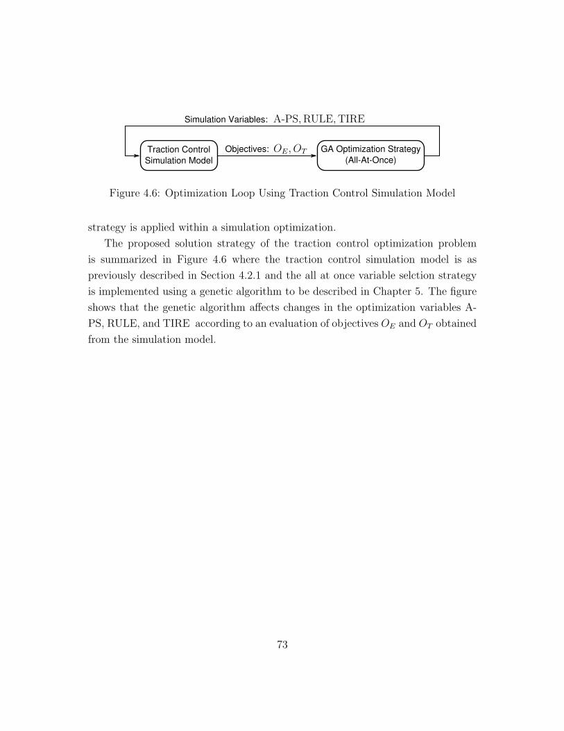
Traction Control
Simulation Model
GA Optimization Strategy
(All-At-Once)
Objectives:
Simulation Variables: A-PS,RULE,TIRE
OE, OT
Figure 4.6: Optimization Loop Using Traction Control Simulation Model
strategy is applied within a simulation optimization.
The proposed solution strategy of the traction control optimization problem
is summarized in Figure 4.6 where the traction control simulation model is as
previously described in Section 4.2.1 and the all at once variable selction strategy
is implemented using a genetic algorithm to be described in Chapter 5. The figure
shows that the genetic algorithm affects changes in the optimization variables A-
PS, RULE, and TIRE according to an evaluation of objectives OE and OT obtained
from the simulation model.
73


Chapter 5
Genetic Algorithm Design
Design details of the genetic algorithm used in the simultaneous plant/controller
optimization of the traction control system are described. First, background on ge-
netic algorithms is presented, including mixed encoding of continuous and discrete
variables and application in fuzzy logic control optimization. Application-specific
design details regarding optimization variable encoding and definition of associated
genetic operations are then provided to define a mixed encoding, multi-chromosomal
genetic algorithm suitable for optimizing the traction control problem summarized
in Section 4.2.4. A novel fuzzy logic rule base encoding is presented to address chal-
lenges in rule base constraint satisfaction associated with search space reduction.
5.1 Genetic Algorithms
Genetic Algorithms (GA) are heuristic optimization methods that were inspired
by Charles Darwin’s principle of natural selection [48]. This principle stems from
the observation that, as a population of species evolves, individuals with beneficial
traits are more likely to survive to reproduce, and hence propagate their traits
to their offspring. GA numerically emulate this process to evolve good solutions
from a population of candidate solutions. As a numerical optimizer, with generally
problem-independent mathematical formulation, a GA possesses intrinsic flexibility
and can equally be applied to problems exhibiting a combination of nonlinear,
75

Initial Population
Selection
Crossover
Mutation
Fitness Evaluation
Initial Fitness Evaluation
Terminating
Condition? Final Population
Yes
NoNew Population
Figure 5.1: Genetic Algorithm Structure [48]
constrained, discontinuous, and multi-modal characteristics [48].
The basic operation of a GA (as presented in Figure 5.1) entails refining a pop-
ulation of candidate solutions through repeated application of a series of genetic
operations consisting of solution selection, crossover, mutation, and fitness evalua-
tion. In the following subsections, the classical operation of a GA on binary strings
is discussed, followed by extensions allowing alternatives to binary encoding, mixed
encoding with multi-chromosomal representation, as well as constrained optimiza-
tion. Parallel implementation strategies that allow high-speed execution of a GA
are also reviewed. This section concludes with a discussion of the application of
genetic algorithms to fuzzy logic controller optimization in the field of genetic-fuzzy
control.
5.1.1 Unconstrained Binary GA
The following sub-sections detail the unconstrained optimization process of a binary
GA with reference to Figure 5.1.
76

Chromosome
Gene
Population
Gene
Figure 5.2: Genes, Chromosomes, and Population
Representation
Prior to the application of a GA, it is assumed that the solution to a given problem
can be represented by a set of variables. Following biological inspiration, each
variable is referred to as a gene and the set of genes forms a chromosome. In
a binary GA, a single chromosome corresponds to a candidate solution to the
problem. A set of candidate solutions forms a population. The relationship
between gene, chromosome, and population is shown in Figure 5.2 where a single
chromosome has been enlarged to show the gene structure. For convenience, a
candidate solution may be referred to as a member of a population. A particular
population may be referred to as a generation to reflect the fact that a new
population is derived from a previous population after every iteration of the GA.
In general, the representation and encoding of variables is problem-dependent.
In a binary GA, it is assumed that all variables are encoded as a string of binary
numbers. For a problem with n variables encoded as genes xi, i = 1 . . . n, a chro-
mosome X is a binary string of length L(X) =∑n
i=1 L(xi), where function L is the
number of bits required to represent its argument. The binary representation allows
the crossover and mutation genetic operators to derive new candidate solutions, or
offspring, from existing candidate solutions, or parents, in a problem-independent
manner.
77

Initial Population
An initial population is instantiated at the beginning of a GA. The initial population
consists of randomly generated candidate solutions [48]. In the case of a binary GA,
a candidate solution is a random binary string of length L(X). The population’s size
is typically fixed during the application of GA. A larger population size increases
the number and diversity of solutions explored but incurs more processing time per
iteration of the GA.
Objective Function and Fitness Evaluation
Every member in the initial population, as well as in subsequent populations, is
subject to a fitness evaluation resulting in a fitness value F used to evaluate
the “goodness” or optimality of the candidate solution for the problem [48]. A
chromosome X with a higher fitness value than another chromosome Y means that
chromosome X represents a solution closer to the optimum than chromosome Y .
Fitness evaluation begins with the use of an objective function to evaluate
the optimality of a chromosome and produce an objective value O. The objective
function is problem-dependent and the variables encoded in the chromosome may
be evaluated by various means ranging from a simple algebraic expression to a large
numerical simulation. In the case of a simulation optimization (Section 4.3.2), and
in this thesis, a simulation model is assumed to evaluate the encoded variables.
Being problem-dependent, the objective value may assume a wide range of num-
bers requiring problem-specific knowledge to interpret. For example, smaller num-
bers represent desirable solutions in minimization problems whereas the converse is
true in maximization problems. Therefore, a mapping Ψ : O → F is introduced to
convert the problem-dependent objective value O to a problem-independent fitness
value F [48].
A common mapping is the ranking scheme used to assign fitness according
to the position ranks of the sorted objective values of a given population [48].
Population members are sorted according to their objective values and the fitness
value is taken as the rank of each member. Higher ranks correspond to higher
fitness and the ascending or descending sort order is chosen depending on whether
78

the optimization is maximizing or minimizing, respectively. The ranking scheme is
affected only by the relative difference in ranking and not by difference in magnitude
of objective values. This mapping characteristic is desirable as discussed in the
following section on the selection process.
Selection
The population is evolved by selectively applying genetic operations that produce a
new generation from members of the current population. Following biological inspi-
ration, new members are preferably derived, or reproduced, from fit members with
the goal of improving the average population fitness towards an optimal solution.
Members are commonly chosen using roulette wheel selection [48] as follows:
1. Sum the fitness values of all population members: Fsum =∑F .
2. Generate a random number r between 0 and Fsum.
3. Return the first population member whose fitness value, when added to the
fitness value of all proceeding population members, is greater than or equal
to r.
This is equivalent to assigning each population member a segment of a roulette
wheel whose size is proportional to the member’s fitness value. Members are selected
for reproduction by uniformly selecting a random point along the circumference of
the roulette wheel and choosing the indicated member.
Example 5.1.1. Assuming a maximization problem and objective values O of 5,
10, 20, 60, 200 for a population of 5 members Xi, i = 1 . . . 5, respectively, the
probability of selecting a given member is shown in Figure 5.3 where Ψ is: a) a
direct mapping F = O (Fsum = 5 + 10 + 20 + 60 + 200), and b) according to the
ranking scheme (Fsum = 1+2+3+4+5). The figure shows that the ranking scheme
is insensitive to differences in magnitude of the objective function and ensures that
one very good solution X5 will not disproportionally dominate the selection process
by occupying a large portion of the roulette wheel [48].
79

2%
3%
7%20%
68%
7%
13%20%
27%
33%
Objective Values (maximization):
Selection Probabilities
a) b)
X1
X1
X2X2
X3X3
X4
X4
X5X5
O(Xi) = 5, 10, 20, 60, 200
Figure 5.3: Roulette Wheel Selection a) Direct Mapping, b) Ranking Scheme [48]
As roulette wheel selection relies on strictly positive fitness values with higher
fitness values corresponding to fitter individuals, it is often paired with an applica-
tion of the ranking scheme during fitness evaluation. The combination allows the
consideration of minimization problems where a smaller objective value corresponds
to higher fitness.
Example 5.1.2. Assume a minimization problem and objective values O of 5, 20,
10, 200, 60 for a population of 5 members Xi, i = 1 . . . 5, respectively. As shown
in Table 5.1, application of a direct mapping F = O leads to an invalid fitness
assignment since the member with the highest objective value is incorrectly assigned
the highest fitness (highest selection probability). In contrast, a valid mapping for
the minimization problem results after sorting objective values in descending order
and applying the ranking scheme such that F = rank and the lowest objective
value is assigned the highest fitness.
Crossover
Members of a new population are derived from existing members using a crossover
process followed by a mutation process. Two parent members A, B are selected
from the current generation, which may include elite members, and a crossover
80

Table 5.1: Example Roulette Wheel Selection on Minimization Problem
Fitness Value F
Rank Member Objective O Direct Map Ranking Scheme
1 X4 200 200 1
2 X5 60 60 2
3 X2 20 20 3
4 X3 10 10 4
5 X1 5 5 5
operation fcross is performed resulting in an offspring C containing genes from both
parents:
C = fcross(A,B). (5.1)
A common crossover operation for binary strings is the one-point crossover
shown in Figure 5.4 [48]. For parent chromosomes A = a1, a2, . . . , aL and B =
b1, b2, . . . , bL with L = L(A) = L(B) bits each, a random crossover point j
is chosen such that the resulting offspring is C = a1, . . . , aj, bj+1, . . . , bL. Al-
though two offspring are generated from each crossover (the other being C ′ =
b1, . . . , bj, aj+1, . . . , aL), only one is kept such that m crossover operations are
needed to produce a population of size m.
Note. Either offspring C or C ′ is discarded depending on the implementation of
the GA. Either offspring may be discarded since the two parents to the crossover
operation are randomly chosen in the selection process.
Mutation
A mutation operation fmutate is applied to each offspring C after crossover to
produce a randomly perturbed offspring D:
D = fmutate(C) (5.2)
Mutation randomly selects and alters a gene with small probability (pm), typically
less than 10% [48]. Bit mutation fmutate is applied to binary strings by randomly
81

1 1 10 0 1 0
Crossover Point
Parents Offspring
1 0 10100
1 1 10
0100 0 1 0
1 0 1
Figure 5.4: Example of One-Point Crossover [48]
1 1 10 1 0 1Original Chromosome
New Chromosome 1 0 10 1 0 1
Bit Mutation
Figure 5.5: Example of Bit Mutation [48]
changing a single bit (Figure 5.5).
Terminating Condition
The cycle of genetic operations is repeated until a terminating condition is reached.
Common choices of termination criteria are a specified number of generations, pre-
defined value of fitness, rate of change of fitness, or a combination of these fac-
tors [48]. Upon termination of a successful GA optimization, the average popu-
lation fitness should have improved with fit candidate solutions approximating an
optimal solution.
Hypothesis Of Operation
The building block hypothesis (BBH) has been proposed to describe the op-
timizing behavior of a GA [48]. The hypothesis assumes the existence of short
sequences of genetic information (or short bit strings in a binary GA) called build-
82

ing blocks that, when present in the encoding of a candidate solution, increases the
fitness of the associated population member. Crossover, as it operates on long se-
quences of genetic material, tends to preserve short building blocks while shuffling
them between population members. Combined with selection, crossover creates
population members consisting of sequences of short building blocks. Crossover is
likely to destroy long building blocks, which negates its benefits. Mutation tends
to generate new building blocks as any portion of the genetic sequence is equally
affected by its action. Hence, BBH offers guidance for the problem-dependent rep-
resentation of optimization variables with encodings that lead to short building
blocks for a successful application of a GA. BBH also motivates modification of the
binary genetic algorithm to accommodate alternative representations as described
next in Section 5.1.2.
5.1.2 Mixed Encodings and Multi-Chromosomal GA
The binary GA of Section 5.1.1 can be classified as a homogeneous GA since
all optimization variables are encoded using the same data type, namely binary.
Further, the binary GA is considered a single-chromosome GA since a candi-
date solution is represented on one chromosome. This section reviews the use of
other data types for encoding, followed by the extension to a mixed-encoding, or
heterogeneous, GA as implemented in multi-chromosomal GA.
Alternative Encodings
The BBH provides motivation to adapt the GA to other data types such as integer,
and floating-point (real-valued) encodings [48]. A motivational example is presented
in Figure 5.6 that illustrates the advantage gained by using an alternative encoding
on the simple optimization problem:
min (x21 + x2
2) subject to: x1, x2 ∈ 0, 1, . . . , 15. (5.3)
The two parameters x1, x2 of this integer optimization problem, with known min-
imum x1 = x2 = 0, can either be encoded as two 4-bit strings or as two integers.
83

Binary Encoding
Integer Encoding
0 1 1 1 1
1 1 1 1
0 15
15
Crossover Point
Parents
Parents
Offspring
Offspring
0 0 1 1
1 1 1 11 1 0 0
Crossover Point
15 15
0 0 0
0 0 0 0
0 0 0 0
0
0 0
Damaged Long Building Block
Preserved Short Building Blocks
= Building BlocksShaded
a)
b)
b1 b2 b3 b4 b5 b6 b7 b8
i1 i2
min (x21 + x2
2) subject to: x1, x2 ∈ 0, 1, . . . , 15
Figure 5.6: Effect of Crossover in a) Binary GA and b) Integer GA
The binary encoding results in longer building blocks corresponding to bit strings
b1b2b3b4 = 0000 and b5b6b7b8 = 0000 for x1 = 0 and x2 = 0, respectively. In con-
trast, integer encoding directly represents the building blocks i1 = 1 and i2 = 0.
For the encoding of two candidate solutions (15, 0) and (0, 15) shown in Figure 5.6,
BBH suggests that a single-point crossover operation in a binary GA is likely to
destroy either building blocks. In contrast, a single-point crossover operation in an
integer GA may lead directly to an optimal solution. In this case, problem-specific
knowledge has allowed a problem decomposition resulting in an integer encoding
leading to smaller building blocks which are not destroyed in crossover. A similar
case applies when comparing a binary GA to a real-valued GA in the continuous
version of (5.3).
In addition to chromosome encoding, it is also required to define appropriate
crossover and mutation operations to manipulate the underlying data type. For
example, the real-valued equivalent to binary crossover is commonly the arith-
metical crossover where a new offspring C is generated by taking the average of
84

the real-valued genes of parents A and B such that [49]:
C =
a1 + b1
2,a2 + b2
2, . . . ,
an + bn2
. (5.4)
Further, Gaussian mutation may be applied to create a real-valued chromosome
D by the addition of a random distribution to a random gene ci of chromosome C
[48]:
D = c1, . . . , ci + ψ(µ, σ), . . . , cn (5.5)
where ci = randomly selected real-valued gene
ψ = Gaussian (normal) random function with mean µ and standard devia-
tion σ.
Mixed Encodings
In the solution of a large problem, a divide-and-conquer approach relies on the
solution of sub-problems leading to the solution of the entire problem. It is nat-
ural to solve each sub-problem using the most efficient technique. For example,
the optimization problem in (5.3) may be viewed as a linear combination of two
sub-problems: minx21 and min x2
2. Assuming the use of a GA, it was shown that
an integer encoding was preferable for both variables x1 and x2 (due to the iden-
tical nature of the sub-problems). In general, a problem may be decomposed into
sub-problems that are best represented by different encodings. Due to coupling be-
tween sub-problems, as demonstrated in Section 4.1, a simultaneous optimization
is required on all sub-problems to find a global optimum [50].
One methodology for breaking down a mixed-encoding problem is to divide
optimization variables into homogeneous groups consisting of the same type [50].
Each group of variables is considered as a separate chromosome Xi in a multi-
chromosomal representation X = X1, X2, . . . , Xm where m is the number of
groups and i ∈ 1 . . .m. In a multi-chromosomal GA, a single candidate solution,
or population member, X is therefore represented by a collection of m homogeneous
chromosomes Xi as shown in Figure 5.7.
85

Chromosomes Genes
PopulationPopulation Member (Candidate Solution)
Figure 5.7: Candidate Solution Representation in Multi-Chromosomal GA
The basic operation of a multi-chromosomal GA remains as shown in Figure 5.1.
Crossover and mutation operations defined for existing homogeneous GAs may be
reused in the matched chromosome mating process of a multi-chromosomal
GA [50]. Population members are considered as ordered sets of chromosomes with
chromosome Ai of A encoding the same variables (with similar encoding type) as
chromosome Bi of B. Hence, the creation of C from A and B can be defined in
terms of (5.1) as:
Ci = fcross(Ai, Bi) (5.6)
where fcross is an appropriate crossover operator for the chromosome type of Ai
and Bi. Similarly, the mutation of a member C to a perturbed D can be defined
in terms of (5.2) as:
Di = fmutate(Ci) (5.7)
where fmutate is an appropriate mutation operator for the chromosome type of Ci.
An extension to the crossover process is obtained by considering the individual
chromosomes of a multi-chromosomal GA as big building blocks, or equivalently,
as solutions to sub-problems. Thus, chromosome shuffling has been proposed in
order to directly exchange, and preserve, solution information at the chromosome
level [51]. Chromosome shuffling creates a new candidate solution C by selecting
chromosomes Ai or Bi from either parent A and B, respectively, with a function
86

Shuffling
Only
Crossover
Only
Shuffling +
Crossover
Parent
Offspring
Offspring
Parent
Chromosome 1 Chromosome 2 Chromosome 3
A
B
C
C ′
Figure 5.8: Chromosome Shuffling and Crossover [51]
fshuffle:
Ci = fshuffle(Ai, Bi). (5.8)
An example definition of fshuffle is to randomly assign Ai or Bi to Ci:
Ci =
Ai, rand( ) < 0.5
Bi, otherwise.(5.9)
where rand( ) returns a uniform random number between 0 and 1. Since chromo-
some shuffling and crossover both operate on two parents, the two may be performed
simultaneously in a single step as shown in Figure 5.8. Two offspring C and C ′ are
generated by chromosome shuffling and crossover, but, as in the case of one-point
crossover, only one offspring C is kept.
5.1.3 Constraint Handling
A GA relies upon the generation of candidate solutions by combining existing so-
lutions through crossover and randomly perturbing existing solutions through mu-
tation. The inclusion of constraints in an optimization problem may lead to the
generation of infeasible solutions that require additional consideration as discussed
in this section.
87

The Feasible Search Space
Consider a general optimization problem (to be solved by GA) of the form:
optimize O(X), (5.10)
where O is an objective function and X (or X for multi-chromosomal GA) is a
candidate solution encoding n optimization variables xi, i = 1 . . . n. As currently
stated, (5.10) is an unconstrained optimization problem where the domain of the
variables defines the search space S of the problem. For example, if X is a
homogeneous encoding of n real-valued variables, then the search space of (5.10) is
the n-dimensional space of real numbers S = Rn.
Definition of genetic operations, thus far, has allowed the GA to generate can-
didate solutions within the entire search space. This is desired for unconstrained
optimization where it is assumed that all X ∈ S are feasible candidate solutions.
The addition of inequality and equality constraints, for example as present in (4.1)
to (4.3), may restrict the set of feasible solutions, or feasible search space F , to
a subset of the search space such that X ∈ F ⊂ S [52]. In Figure 5.9, candidate
solutions A and B are within the feasible search space with an optimum solution of
X. The figure illustrates that constraints may produce a disjoint, nonconvex fea-
sible search space. It is then possible that genetic operations may create infeasible
candidate solutions C within the infeasible search space U which is defined as
the complement of F . The remaining discussion is focused on proposed methods
[52] for dealing with infeasible candidate solutions generated by constraints. The
methods may be broadly classified as either rejecting, avoiding, or incorporating
infeasible solutions into the GA.
Rejection
Perhaps the simplest approach is to discard infeasible candidate solutions from the
population and reapply the selection process to generate an alternative candidate.
This method works but is disadvantageous when the feasible search space F is small
compared to the search space S. In addition to the computational overhead of gen-
erating alternatives to an infeasible solution, the infeasible candidate solutions may
88

Search Space
Infeasible Search Space
Feasible Search Space
S
F
U
A
B
CX
Figure 5.9: Search Space with Feasible and Infeasible Parts [52]
contain building block information that should be not be discarded. For example,
in Figure 5.9, infeasible candidate solution C may allow the feasible candidate A
to “cross” an infeasible region to reach the solution optimum X [52].
Searching Domain
The method of searching domain requires no modification to an unconstrained GA
as it involves restating the optimization itself such that the feasible search space
becomes equivalent to the search space F = S [48]. Careful selection, or novel
introduction, of variable encoding techniques may remove constraints required in
alternative representations.
Example 5.1.3. Suppose a variable x is constrained to the natural numbers
0, 1, . . . , 7. An integer encoding with the constraint that 0 ≤ x ≤ 7 satisfies
optimization requirements. However, the constraint can be eliminated from the
solution process if the variable is alternatively encoded as a 3-bit binary string
whose search space is equal to the feasible search space (binary numbers 000 to 111
map to integers 0 to 7).
Repair Mechanism
Repair algorithms are implemented when it is relatively easy to change an infea-
sible candidate solution C into a feasible candidate solution A [52]. The repaired
89

candidate solution A may replace the original C in the population, or the repair
may be done only for fitness evaluation and leave C within the population. The re-
pair mechanism is typically inserted in-between the mutation and fitness evaluation
steps of Figure 5.1. Since fitness evaluation is typically the most computationally
intensive process of a GA [48], the computational overhead associated with repair
is acceptable as it allows the GA to focus on exploring the feasible search space.
Example 5.1.4. Assume a variable is constrained to the natural numbers 0, 1, . . . , 5
and represented by a 3-bit binary encoding. A 3-bit binary representation is nec-
essary to include the feasible search space F = 000, 001, 010, 011, 100, 101. How-
ever, candidate solutions “110”, “111” violate the constraint and are therefore in-
feasible. A repair mechanism may be implemented to map the infeasible candidates
into the feasible search space by taking their complements such that 110 → 001
and 111 → 000.
Specialized Genetic Operations
Under the assumption that the initial population is within the feasible search space,
the crossover and mutation operations may be designed as a closed set of oper-
ations to maintain the feasibility of solutions. Such specialized genetic operations
have been demonstrated for convex feasible search space however the method is cur-
rently unable to deal with nonconvex search spaces (and hence nonlinear constraints
in general) [52].
Example 5.1.5. Assuming candidate solutions A and B, with real-valued encoding
and within a convex feasible search space, arithmetical crossover (5.4) A+B2
always
produces feasible offspring C. A closed set definition of mutation on C is to ran-
domly choose a point on a line with random slope passing through C. The choice
of the point is restricted to within the segment defined by two points of intersection
of the line with the boundary of the convex search space [52].
90

Penalty Scheme
Various penalty schemes have been proposed to allow the direct inclusion and eval-
uation of infeasible candidate solutions within a population [52]. Consideration in
penalty scheme design involve methods to compare two infeasible members as well
as an infeasible member to a feasible member. For a problem with m constraints,
a corresponding number of constraint violation measures fj, j = 1 . . .m are
introduced to allow such comparisons. Constraint violation measures are associ-
ated with penalties that decrease the fitness of a candidate solution depending on
a combination of how many or by how much constraints are violated.
The penalty scheme does not guarantee that the final solution found will be
within the feasible search space, although it is the intent of penalties to minimize
constraint violation through the selection process. This method may permit a
small violation of a constraint to allow a large gain towards an optimal solution.
However, the penalty scheme can incur much computational overhead in evaluating
infeasible candidates when the feasible search space is much smaller than the search
space [48].
Example 5.1.6. Assume a minimization problem with m constraints and objective
function O(X) that evaluates both feasible and infeasible candidate solutions X. A
simple penalty scheme is obtained through a weighted combination of the objective
function and the number of violated constraints to produce a modified objective
function O′ [48]:
O′(X) = O(X) + δm∑
i=1
fj(X)
where m = number of constraints
δ = penalty coefficient (positive for minimization problems)
fj =
1, constraint m violated by X
0, otherwise.
91

5.1.4 Parallel Architecture
The structure of a GA (Figure 5.1) allows various methods of parallelization [48].
In general, a parallel implementation of a GA utilizes multiple computational nodes
connected by a communication network to perform the time consuming, yet inde-
pendent, crossover, mutation, and fitness evaluation operations.
The Global GA implementation is based on a farmer-worker architecture (Fig-
ure 5.10). The farmer node selects pairs of population members to send to worker
nodes for crossover, mutation and fitness evaluation, and collects the results as well
as the new offspring. This information allows the farmer to create the next gener-
ation and repeat the selection process. A disadvantage of the Global GA is that
workers are idle while the farmer is doing the selection process which may involve
sorting and ranking the results. A global GA implementation is implemented in
this thesis.
Other parallelization schemes require some modification to the basic operation of
the GA. In migration GA, also called coarse grained parallel GA, the population is
divided into sub-populations. Each sub-population is then evolved separately using
a conventional GA on a dedicated node. A migration operation is introduced
to allow fit candidate solutions to move between sub-populations and ultimately
spread within the whole population. Migration GA apply to small multi-processor
clusters (i.e. a small number of high performance nodes) since a small number of
sub-populations are evolved on dedicated nodes [48].
In contrast, on large clusters with many nodes, a diffusion GA, also called
a fine grained parallel GA, assigns each population member to a single dedicated
node [48]. The node performs a modified selection process in addition to regular
crossover, mutation, and fitness evaluation for a single member. Unlike a global
GA, selection is distributed within the cluster. Each node, however, is limited to
selecting between a restricted number of immediately adjacent nodes (or members)
on the cluster’s communication network. The limitation on adjacent nodes allows
the practical implementation of communication networks on massively parallel com-
puters. For example, nodes of a diffusion GA may be connected by a high-speed,
rectangular grid communication topology that limits adjacent nodes to four.
92

Farmer
Worker 1
Selection
Crossover
Mutation
Fitness Evaluation
Worker 2
Crossover
Mutation
Fitness Evaluation
Worker 3
Crossover
Mutation
Fitness Evaluation
Exchange
Parents and Offsping
Figure 5.10: Global GA [48]
5.1.5 Genetic-Fuzzy Control
Previous discussion of fuzzy logic control in Section 3.2 and the current discussion
of GA have established their individual flexibility and broad-applicability in control
and optimization problems, respectively. A fuzzy logic controller presents a general
control structure with many parameters required in the definition of membership
functions and rule base. Fuzzy logic controller parameters are typically chosen
by intuition derived from real-world experience and therefore not optimal. As
briefly mentioned in Section 3.2.7, the optimization of fuzzy logic controllers is
difficult due to the nonlinear control action of fuzzy logic, the large search spaces
involved (as a result of numerous parameters), and the mix of continuous and
discrete parameters. Researchers have therefore relied upon genetic algorithms as
a highly problem-independent, general framework for the nonlinear optimization of
fuzzy logic controllers termed genetic-fuzzy control [6].
Automotive applications of genetic-fuzzy control have focused on the use of a
single-chromosome binary GA (Section 5.1.1) to optimize the shape of membership
functions while assuming a fixed, potentially non-optimal rule base [6][39]. In both
works, continuous triangular membership function parameters, including prototype
location and span, are discretized and encoded as binary strings. The controller
parameters are treated as optimization variables in a simulation optimization in-
volving the system under consideration (being a hybrid electric vehicle powertrain
[6], and an active vehicle suspension [39]). Both works conclude that genetic-fuzzy
93

control is effective at determining the shape of membership functions.
The flexibility of a GA design permits both membership functions and rule base
to be optimized simultaneously [48]. In this approach, traditional control objectives
are supplemented by objectives to minimize the number of membership functions
and rules in the optimized controller.
Continuous variables are required to define the shape of membership functions
in addition to the following discrete variables for the definition of the rule base:
• Number of membership functions associated with the universe of each input.
• Number of membership functions associated with the universe of each output.
• Conclusion associated with the premise in each rule.
These variables allow the optimization of a rule base to be decomposed into the
optimization of the conclusion of existing rules as well as the optimization of the
number of rules as clarified in Example 5.1.7.
Example 5.1.7. Assume a double-input, single-output fuzzy logic controller with a
rule base represented by a FAM table. Let nx1, nx2, ny be the number of membership
functions associated with the universe of inputs x1, x2 and output y, respectively.
For nx1 = 3, input x1 may be fuzzified using membership functions representing
various degree of “cold”, “warm”, and “hot”. For nx2 = 2, input x2 may be fuzzified
using membership functions representing various degree of “slow” and “fast”. For
ny = 4, output y may be defuzzified using membership functions representing
various degree of “tiny”, “small”, “med(ium)”, and “large”. An initial set of 6
(arbitrary) rules is given by the FAM table shown in Figure 5.11a.
The conclusions of existing rules may be modified by assigning new entries
within the FAM table as in Figure 5.11b. Note that the conclusion “huge” in
response to premise “x1 is hot and x2 is slow” is made possible by the addition of
membership function “huge” to the output universe such that ny = 5.
The number of rules is directly affected by the number of membership functions
associated with the universe of each input. In Figure 5.11c, the FAM table describes
9 rules since nx2 has been increased to 3 with the addition of membership function
“faster” to the input universe of x2.
94

cold warm hot
slow
fast
tiny small
med large
huge
cold warm hot
slow
fast
cold warm hot
slow
fast
faster
med
large
tiny
large
med
small med
med hugetiny
largesmall med
tiny small med
a) b) c)
x1
x1x1x2
x2x2
Figure 5.11: Rule Base Optimization Variables a) Initial Rule Base, b) Rule Con-
clusions, c) Number of Rules
Due to difficulties in encoding a rule base of varying size, the minimization of
the number of rules requires a non-standard extension to the GA as shown in Fig-
ure 5.12 [48]. The figure shows that the minimization of the number of rules used by
a genetic-fuzzy controller requires a separate population containing rule sets of all
possible sizes. For example, the rule base population of Figure 5.11a would contain
(nx1 − 1) × (nx2 − 1) × (ny − 1) = 6 members where each member corresponds to
a rule base with unique nx1, nx2, ny and assuming nx1, nx2, ny > 1 to ensure inputs
and outputs are associated with more than one membership function. A particular
rule base is selected according to rule base parameters encoded within members of
a population encoding the shape and number of membership functions. The GA
structure presented in Figure 5.12 ensures that, prior to fitness evaluation, a con-
troller is synthesized with a rule base sized in agreement with the encoded definition
of membership functions. Applications of the proposed optimization scheme to a
water pump system and a solar heating plant have demonstrated that desired sys-
tem performance can be maintained while the number of rules is minimized through
appropriate selection of rule conclusions and membership functions [48].
Although a worthwhile consideration, the minimization of rule base size is not
considered in this thesis since the proposed extension to the GA of Figure 5.11 is
problem-specific to the design of genetic-fuzzy controllers. This is in conflict with
the current desire to develop a generalized simultaneous plant/controller optimiza-
tion framework which may incorporate other forms of controllers. However, without
modification to the basic GA structure of Figure 5.1, this thesis does consider an
optimization over the numerous permutations of the possible conclusions associated
95

Membership
Function
Population
Rule Base
Population
SelectionCrossover
+ Mutation
Extract Encoded
Rule Base Size
Select Rule Base
of Appropriate Size
Mutate Rule Base
Fitness Evaluation
Extract Encoded
Membership Functions
New Membership Function Chromosome
Start
GA Extension
Figure 5.12: GA for Membership Function & Rule Base Optimization [48]
with a given premise in a rule base of fixed size as detailed in Section 5.3.3.
5.2 GA in Traction Control System Optimization
A mixed encoding, multi-chromosomal GA is selected to optimize the traction con-
trol system since the problem includes a mixture of continuous and discrete vari-
ables. This section describes design details that adapt the general description of the
mixed encoding GA of Section 5.1.2 to the traction control optimization problem
summarized in Section 4.2.4. With reference to the structure of the mixed encoding,
multi-chromosomal GA shown in Figure 5.13, the following discussion describes: the
encoding of optimization decision variables within population members, the fitness
evaluation and selection process based on candidate solutions associated with low
drive cycle energy use OE and completion time OT , the combined chromosome shuf-
fling and crossover operation, and the multi-chromosomal mutation operation. To
simplify the GA implementation, the optimization process terminates after a fixed
number of generations are produced.
96
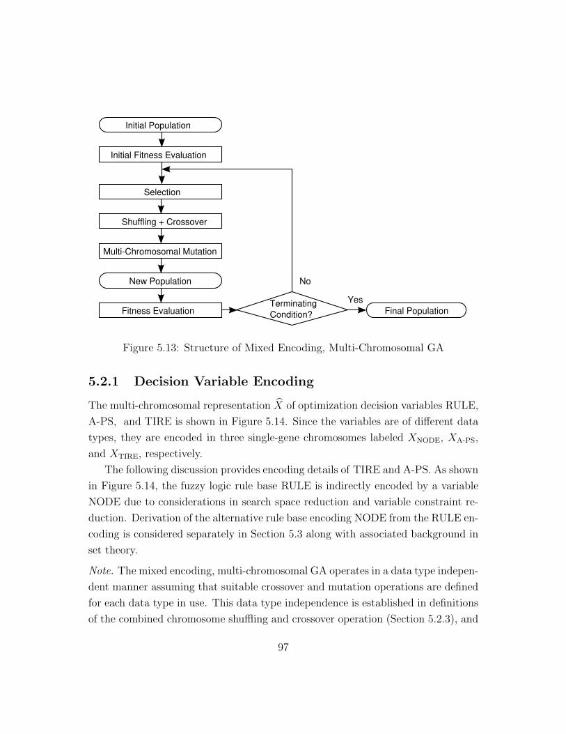
Initial Population
Selection
Shuffling + Crossover
Multi-Chromosomal Mutation
Fitness Evaluation
Initial Fitness Evaluation
Terminating
Condition? Final Population
Yes
NoNew Population
Figure 5.13: Structure of Mixed Encoding, Multi-Chromosomal GA
5.2.1 Decision Variable Encoding
The multi-chromosomal representation X of optimization decision variables RULE,
A-PS, and TIRE is shown in Figure 5.14. Since the variables are of different data
types, they are encoded in three single-gene chromosomes labeled XNODE, XA-PS,
and XTIRE, respectively.
The following discussion provides encoding details of TIRE and A-PS. As shown
in Figure 5.14, the fuzzy logic rule base RULE is indirectly encoded by a variable
NODE due to considerations in search space reduction and variable constraint re-
duction. Derivation of the alternative rule base encoding NODE from the RULE en-
coding is considered separately in Section 5.3 along with associated background in
set theory.
Note. The mixed encoding, multi-chromosomal GA operates in a data type indepen-
dent manner assuming that suitable crossover and mutation operations are defined
for each data type in use. This data type independence is established in definitions
of the combined chromosome shuffling and crossover operation (Section 5.2.3), and
97

(Poset Node #) (Real-Coded) (1-bit Binary)
Chromosome Chromosome Chromosome
Fuzzy Logic Controller Variables Vehicle Variable
Single Gene Single Gene Single Gene
Candidate Solution
NODE ∈ 1, ..., 84 A-PS ∈ [0.2, 0.8] TIRE ∈ 0, 1
XNODE XA-PS XTIRE
X
Figure 5.14: Encoding of Traction Control System Design Variables
the multi-chromosomal mutation operation (Section 5.2.4).
TIRE Encoding
Since TIRE is constrained between the selection of either a performance tire or a
low rolling resistance tire, it is encoded as a single bit binary gene in chromosome
XTIRE. Binary one-point crossover and bit mutation operations are defined on
XTIRE as described in Section 5.1.1 although they exhibit degenerate operation on
TIRE since XTIRE consists of a single bit.
Given single-gene binary chromosome parents ATIRE and BTIRE, the crossover
operation degenerates to the simple assignment CTIRE = ATIRE (assuming that the
implementation discards the alternative offspring C ′TIRE = BTIRE). An implementa-
tion may consistently discard either offspring since the two parents to the crossover
operation are randomly chosen in the selection process.
Mutation of the single-gene binary chromosome CTIRE causes TIRE to invert
and therefore toggles tire selection between the performance tire and the low rolling
resistance tire.
A-PS Location Encoding
Since A-PS represents the location of the Positive-Small adhesion gradient mem-
bership function over a continuous range of values, it is real-coded as a floating
98

point number.
Arithmetic crossover on two single-gene parents AA-PS and BA-PS is defined as
in (5.4) but degenerates to the average of A-PS stored in both parents such that
offspring CA-PS =AA-PS +BA-PS
2.
Gaussian mutation on offspring CA-PS is defined in Equation (5.5) and, in the
case of a single-gene chromosome, produces a perturbed chromosome DA-PS =
CA-PS + ψ(0, σ) such that a random number is added to A-PS with a distribution
defined by Gaussian function ψ with zero mean and standard deviation σ.
Due to the constraint A-PS ∈ [0.2, 0.8] and the fact that ψ has an unbounded
range and can return large values with small probability, a repair mechanism is
required to prevent an out-of-bounds assignment to A-PS. Simply saturating a
mutation to the lower and upper bounds allowed for A-PS would greatly increase the
occurrences of mutations resulting in A-PS being assigned a minimum or maximum
limit. To avoid this, a repair on an out-of-bounds mutation is done by “bouncing”
[53] the mutation back within the allowable range by first saturating the sum of
CA-PS +ψ(0, σ) to the bounds of A-PS while retaining the remainder exceeding the
violated bound. The negative of the remainder is then added back to the sum and
the process is repeated until the remainder is zero.
Example 5.2.1. Assume A-PS ∈ [0.2, 0.8]. If CA-PS = 0.3 and a Gaussian mutation
results in a change of ψ(0, σ) = −0.9, then the sum 0.3 + (−0.9) is saturated to
the lower bound of A-PS to produce the intermediate result C ′A-PS = 0.2 and the
remainder exceeding the lower bound is -0.8. The negative of the remainder is then
added to C ′A-PS. The sum (C ′
A-PS +0.8) is saturated to the upper bound to produce
the intermediate result C ′′A-PS = 0.8 with a remainder of 0.2. The final addition
of the negative of the remainder to C ′′A-PS produces the final mutation assignment
DA-PS = 0.8 − 0.2 = 0.6 that satisfies the constraint on A-PS.
5.2.2 Fitness Evaluation and Selection
The fitness of each member X within the population is evaluated by first config-
uring the traction control system model according to the design variables encoded
99

in X and simulating system dynamics to evaluate the drive cycle energy use OE
and completion time OT objectives. The system-level objective value Os is then
evaluated using the weighted sum of OE and OT as defined in (4.12). After Os is
evaluated for all members within the population, the ranking scheme is applied by
sorting members in descending order according to Os such that members with lower
Os are assigned a higher rank and fitness. Therefore, members are assigned fitness
values appropriate for the minimization of Os. For each member to be generated
in the new population, roulette wheel selection is applied twice to select the parent
members for the subsequent combined shuffling and crossover operation.
5.2.3 Chromosome Shuffling and Crossover
Chromosome shuffling is implemented as a one-point shuffle that is analogous
to the one-point crossover operation. For two parent members with a multi-
chromosomal representation A = A1, A2, . . . , Am and B = B1, B2, . . . , Bm of
length m, a random crossover point j ∈ 1, . . . ,m is chosen such that a one-point
shuffle about j results in child C = A1, . . . , Aj, Bj+1, . . . , Bm.
Although shuffling and crossover can be done simultaneously as illustrated in
Figure 5.8, in this thesis only one is randomly performed when generating an off-
spring from two parents A and B. As shown in Figure 5.15, a chromosome j is
randomly selected and, with equal probability, either a one-point shuffle is per-
formed about chromosome j or a one-point crossover is performed on chromosome
j to produce offspring C. This definition of the shuffling and crossover operation
allows the GA to consider: sequences of chromosomes as building blocks when shuf-
fling is performed, or sequences of genes within a chromosome as building blocks
when crossover is performed.
Note. Recall from the building block hypothesis (Section 5.1.1) that building blocks
are short sequences of genetic information that, when present in an encoding, in-
crease the fitness of the associate population member.
As defined, the shuffling and crossover operation is independent from the under-
lying chromosome data types of the parent members. Either an entire chromosome
100

Parent
Parent
Random Shuffle or Crossover
Select Random Chromosome
Offspring
by Shuffle
Offspring
by Crossover
A
B
CC
Figure 5.15: Random Chromosome Shuffle or Crossover Operation
is exchanged in the shuffling operation, or the crossover operation of the chromo-
some is invoked by the shuffling and crossover operation of the mixed encoding,
multi-chromosomal GA. Hence, the shuffling and crossover operation can be ex-
tended to support new chromosome data types provided that a crossover operation
is defined on the data type.
5.2.4 Multi-Chromosomal Mutation
The mutation of a member consisting of a multi-chromosomal representation pro-
ceeds by choosing a random chromosome within the member and invoking the
appropriate mutation operation depending the chromosome’s data type. Unlike
the shuffling and crossover operation that must be performed to generate each off-
spring of a new population, the multi-chromosomal mutation operation is applied
to an offspring with a small mutation probability pm.
The mutation probability pm is chosen large enough such that new building
blocks may be produced through mutation. However, excessive mutation may also
destroy existing building blocks. For this reason, the multi-chromosomal mutation
is defined such that a change occurs in a single chromosome of a multi-chromosomal
representation. This is in contrast to the definition of the mutation process defined
101

Member
Mutate Random Chromosome
Perturbed
Member
Mutation
C
D
Figure 5.16: Multi-Chromosomal Mutation
in (5.7) where each chromosome in the multi-chromosomal representation is mu-
tated.
Multi-chromosomal mutation is shown in Figure 5.16 where a single chromo-
some of member C is mutated to produce a perturbed member D. As defined, the
multi-chromosomal mutation operation is independent from the underlying chromo-
some data types of member C since the operation invokes the mutation operation
associated with the data type. The multi-chromosomal mutation operation can be
extended to support new chromosome data types provided that a mutation opera-
tion is defined on the data type.
Since the shuffling and crossover operation and the multi-chromosomal mutation
operation are responsible for generating new candidate solutions, their indepen-
dence from chromosome data types allows the mixed encoding, multi-chromosomal
GA to be extended to support a new data type provided that crossover and mu-
tation operations can be defined on the data type. This property is exploited in
Section 5.3 to define a novel encoding for the fuzzy logic rule base.
5.3 Novel Fuzzy Logic Rule Base Encoding
Motivation for a novel fuzzy logic controller rule base encoding is obtained by
considering a simple and direct encoding of rule base conclusions as independent
integers. The direct encoding leads to exponential growth of the search space with
the number of rule base entries. For example, encoding the 6 rule base conclusion
102

variables Ci from RULE of the traction controller results in a search space with
4096 = 46 rule base configurations since each of the variables may assume any of 4
possible conclusions according to (4.9).
To reduce the search space, application-specific knowledge may be used to derive
constraints on allowable rule base configurations. For the traction control system,
the constraints in (4.10) are intuitively derived to admit only those that tend to
prescribe an increase in torque output Ta as input torque request Tref and adhe-
sion gradient A increase. However, such constraints may create a large difference
in size (large infeasible search space) between the search space that exists prior
to constraint application and the smaller feasible search space defined by the con-
straints. As described in Section 5.1.3, a constraint handling mechanism must then
be incorporated in the optimizing GA to deal with infeasible solutions that violate
constraints.
In the current optimization of the traction control system, the rule base is heav-
ily constrained by (4.10) (to be quantified in the encoding analysis of Section 5.3.3)
to produce a small feasible search space and, consequently, a large infeasible search
space. With the direct rule base encoding, constraint handling methods such as re-
jection and the penalty scheme are undesirable due to high computational overhead
associated with simulating infeasible solutions. It is also currently not obvious how
to repair an infeasible rule base definition. Thus the direct rule base encoding leads
to challenges in either exploring a large search space, or reducing computational
overhead associated with evaluating infeasible solutions.
An alternative and novel encoding of rule base conclusions is therefore proposed
to evolve an optimal rule base configuration within a constrained search space
while avoiding infeasible solutions. Minimal background in set theory is presented
to enable the definition of a partial ordering of “monotonic increasing” matrices.
The partial ordering, termed a partial ordering by delta inclusion, is then applied
to encode the rule base for use in the mixed-encoding, multi-chromosomal GA
previously described in Section 5.2.
103

Table 5.2: Preliminary Set Theory Notation [54]
Notation Meaning
a = b “a” and “b” denote the same thing
a 6= b “a” and “b” denote different things
a ∈ S “a” is an element of set “S”
P ⇒ Q If “P” then “Q” (“P” implies “Q”)
∀ “for all”
∃ “there exists”
3 “such that”
P (x) A statement P in the variable x
⇔ “If and Only if”
A ⊆ B “set A is a subset of set B”
5.3.1 Set Theory
This section reviews the set theory required to define a lattice. All definitions in
this section are taken from [54] unless stated otherwise.
Definition 5.3.1. A set is a collection of objects. These objects may be physical
or abstract. Most mathematical objects can be defined in terms of sets including
points, numbers, and operations.
Set theory formalizes the expressive power of sets and, as such, is part of the
foundation for mathematics [54]. Table 5.2 reviews set theory notation used in this
section. Set theory notation is used to abbreviate statements in set theory. For
example, the subset statement A ⊆ B is an abbreviation for the statement:
∀x, x ∈ A⇒ x ∈ B.
Definition 5.3.2. Given a set S, the power set of S, denoted by X = [S], is a
set where:
∀x, x ∈ [S] ⇔ x ⊆ S.
104

The power set of S is therefore a set whose elements x ∈ X are all the possible
subsets of S. In other words, the elements x of a power set are themselves sets.
Therefore, in this case, x carries a double meaning of an element x ∈ X and of a
set x ⊆ [S].
Definition 5.3.3. Given two sets A and B, an ordered pair is denoted as (a, b)
where a ∈ A and b ∈ B. Ordered pairs have the property that:
(a, b) = (c, d) ⇔ a = c, b = d, a, c ∈ A, b, d ∈ B.
Definition 5.3.4. The cartesian product of two sets A and B is defined as:
A×B = (a, b)| a ∈ A, b ∈ B.
The cartesian product A × B is therefore a set containing all ordered pairs
formed from elements of sets A and B.
Definition 5.3.5. Given two sets A and B, and the subset f of A× B, then f is
a mapping of A onto B if:
1. For each a ∈ A, ∃ b ∈ B 3 (a, b) ∈ f .
2. (a, b) ∈ f and (a, c) ∈ f ⇒ b = c.
In the mapping of A onto B, each element of A is assigned to exactly one element
of B. The mapping f may also be called a function or transformation. Also,
the notation afb means (a, b) ∈ f .
Definition 5.3.6. A relation F from set A to set B is any subset of A×B.
If elements a ∈ A and b ∈ B are in a relation F , then (a, b) ∈ F . Also, (a, b) ∈ F
is abbreviated as aFb. A relation can be considered as a rule that assigns to each
a ∈ A to zero or more elements b ∈ B. A mapping can therefore be interpreted as
a special case of a relation since each element of A is assigned to one element of B.
The sets A and B can be different sets or refer to the same set X. When A and
B refer to the same set, the relation F from A to B is called a relation F on set X.
105

Definition 5.3.7. A partial ordering defined on a set X is a relation F on X
satisfying the following three properties:
1. Relexivity: aFa, ∀ a ∈ X.
2. Antisymmetry: (aFb and bFa) ⇒ a = b, ∀ a, b ∈ X.
3. Transitivity: (aFb and bFc) ⇒ aFc, ∀ a, b, c ∈ X.
A set with a defined partial ordering is termed a partially ordered set or poset
[55]. In general, a ≤ b can be written for aFb when (a, b) is a member of a partial
ordering. If, additionally, a 6= b then a < b may be written [54]. Elements a, b ∈ X
are comparable if either a ≤ b or b ≤ a. In a partial ordering, it may be the case
that two arbitrary elements a, b are not comparable [55].
Note. In set theory, the symbol “≤” denotes any relation F that can be used to
partially order an abstract set X as defined above. Hence the use of “≤” in set
theory is not limited to the “usual” use in ordering sets of numbers. However, for
the particular case whereX represents a set of numbers (for exampleX = R, the set
of real numbers), the symbol “≤” in “a ≤ b” represents a particular partial ordering
where the statement a ≤ b can be writen when (a, b) ∈ “≤” ⇔ the numerical value
of a is less than or equal to the numerical value of b, a, b ∈ R. This leads to the usual
interpretation of a ≤ b when applied to numbers. In this thesis, the meaning of “≤”
is inferred by context and will denote either an abstract relation when applied to
general sets, or the usual numerical ordering operation when applied to numbers.
Similar consideration should be given to the use of the symbol “<”.
Example 5.3.1. Partial ordering by inclusion is a common example of partial
ordering and is defined as a relation F on the power set of S as follows: Given
the power set X = [S], the relation F on X is such that (A,B) ∈ F ⇔ A ⊆
B, A,B ∈ X. Therefore, if A ⊆ B, then (A,B) is a member of a partial ordering
by inclusion and A ≤ B may be written [54]. Intuitively, set A is smaller or equal
than set B since it contains fewer or equal elements and, in this way, the elements
of a power set can be partially ordered.
106

The partial ordering between elements in a poset X can be visualized in a type
of directed graph called a Hasse diagram. In a Hasse diagram, nodes correspond
to elements x ∈ X and edges to pairs (x, y) with x < y, x, y ∈ X. Edges are
drawn as rising lines from a “lower” node x to a “higher” node y to indicate x < y.
To simplify the Hasse diagram, edges are only drawn for “neighboring” x, y [55].
Example 5.3.2. The partial ordering by inclusion of the power set of S = a, b, c
is shown in the Hasse diagram of Figure 5.17. The following steps were used to
derive the graph:
1. The power set of S is X=[S]=a, b, c, a, b, a, c, b, c, a, b, c, ∅.
There are 8 elements in X and each corresponds to a node in Figure 5.17.
2. A partial ordering is defined as a relation F on X where F is a subset of
X × X. Since X is partially ordered by inclusion, the elements of F are
ordered pairs (A,B) where A ⊆ B and A,B ∈ X. Specifically:
F = (a, b, c, a, b, c), (a, b, a, b, c), (a, c, a, b, c), (b, c, a, b, c),
(a, a, b, c), (b, a, b, c), (c, a, b, c), (∅, a, b, c),
(a, b, a, b), (a, a, b), (b, a, b), (∅, a, b),
(a, c, a, c), (a, a, c), (c, a, c), (∅, a, c),
(b, c, b, c), (b, b, c), (c, b, c), (∅, a, b),
(a, a), (∅, a), (b, b), (∅, b), (c, c), (∅, c), (∅, ∅).
3. Edges are drawn between nodes A and B to indicate A < B. Only edges
between “neighboring” A,B are drawn. For example, although node a is
a subset of each of nodes a, b, a, c, and a, b, c, edges are drawn only
between it and its neighbors a, b and a, c. The fact that a ⊆ a, b, c
is implied by the edges between a, b - a, b, c and a, c - a, b, c.
Definition 5.3.8. Given a poset X and elements x, y ∈ X, an element a ∈ X is
a lower bound for x and y if a ≤ x and a ≤ y. Multiple lower bounds may exist
107

a, b, c
a, b a, c b, c
a b c
∅
Figure 5.17: Example Hasse Diagram of a Partially Ordered Set by Inclusion [55]
for x and y. However, a greatest lower bound, or meet, l ∈ X for x and y may
exist, and is unique if so. An element l ∈ X is defined as a meet when [55]:
l ≤ x and l ≤ y (l is a lower bound for x and y),
(∀ a ∈ X) a ≤ x and a ≤ y ⇒ a ≤ l
(l is greater than other lower bounds for x and y).
Definition 5.3.9. Similarly, an element b ∈ X is an upper bound for x and y
if x ≤ b and y ≤ b. Multiple upper bounds may also exist for x and y. A least
upper bound, or join, u ∈ X may exist, and is unique if so. An element u ∈ X
is defined as a join when [55]:
x ≤ u and y ≤ u (u is an upper bound for x and y),
(∀ b ∈ X)x ≤ b and y ≤ b⇒ u ≤ b
(u is less than other upper bounds for x and y).
Definition 5.3.10. A lattice is a special case of a poset and occurs when the
meet and join of any two elements of the poset always exist. Given a lattice L, the
meet of two elements x, y ∈ L is written as x ∧ y, and the join of the elements as
x ∨ y [55].
108

Example 5.3.3. The partial ordering by inclusion of [S] is a lattice [55]. Intuitively,
this is because the meet and join operators, ∧ and ∨, are equivalent to the set union
and intersection operators, ∩ and ∪, respectively. The intersection of two sets is the
biggest set that contains elements common to both sets (meet). The union of two
sets is the smallest set that contains all elements of both sets (join). For example,
in Figure 5.17:
a, b ∧ a, c = a = a, b ∩ a, c
and
a ∨ b, c = a, b, c = a ∪ b, c.
5.3.2 Novel Partial Ordering by Delta Inclusion
This section builds on Section 5.3.1 to define a novel partial ordering on a set termed
“partial ordering by delta inclusion (poset by delta inclusion).” The mechanism of
delta inclusion is similar to that of subset inclusion in that both rely on the notion
that certain elements of X “contain” other elements of X. In contrast to subset
inclusion where sets “contain” other sets, delta inclusion relies on the idea that
matrices “contain” other matrices. The remainder of this section describes posets
by delta inclusion. First, a mechanism to compare particular matrices is defined.
Then the construction of X and the relation F on X are considered with respect
to posets by delta inclusion.
Consider an m × n matrix, Em×n, with entries ei,j for all 1 ≤ i ≤ m and
1 ≤ j ≤ n:
e1,1 . . . e1,n
.... . .
...
em,1 . . . em,n
=[ei,j
], ∀ i = 1..m, j = 1..n.
Definition 5.3.11. Define a monotonic increasing matrix, Em×n, as a matrix
109

with non-decreasing components from the set of natural numbers:
ei,j ∈ 1, 2, 3, ..., i = 1..m, j = 1..n
ei,j ≤ ei,j+1, i = 1..m, j = 1..(n− 1)
ei,j ≤ ei+1,j, i = 1..(m− 1), j = 1..n.
That is, each entry of a monotonic increasing matrix is a natural number and
is less than or equal to entries immediately to the right, below, and diagonally to
the right and below.
Example 5.3.4. Examples of monotonic increasing matrices are:
[2 2
3 3
],
[1 2
3 3
], and
[1 1
1 1
].
Definition 5.3.12. Given two monotonic increasing matrices, Am×n, Bm×n, define
the delta inclusion operator “b” as:
Am×nb Bm×n ⇔ (ai,j ≤ bi,j, ∃ ai,j < bi,j) ∀ i = 1..m, j = 1..n.
Similar to the subset operator ⊆, the delta inclusion operator b invokes the
notion of “containment.”
Example 5.3.5. By delta inclusion, it can be said that:
[1 2
3 3
]b
[2 2
3 3
]and
[1 1
1 1
]b
[1 2
3 3
].
Definition 5.3.13. Define the delta set of a monotonic increasing matrix Tm×n,
written 〈Tm×n〉, as a set that includes all monotonic increasing matrices Em×n
where:
∀Em×n, Em×n ∈ 〈Tm×n〉 ⇔ Em×nb Tm×n.
Example 5.3.6. For example, given T 2×2 =
[2 2
3 3
], then the delta set of T 2×2 is
110

the set of 14 possible monotonic increasing matrices:
X = 〈T 2×2〉 =
⟨[2 2
3 3
]⟩=
[2 2
3 3
],
[1 2
3 3
],
[2 2
2 3
],
[1 1
3 3
],
[1 2
2 3
],
[2 2
2 2
],
[1 1
2 3
],
[1 2
1 3
],
[1 2
2 2
],
[1 1
1 3
],
[1 1
2 2
],
[1 2
1 2
],
[1 1
1 2
],
[1 1
1 1
].
Definition 5.3.14. Given a delta set X = 〈Tm×n〉, a partial ordering by delta
inclusion is defined as a relation F on X such that:
(Am×n, Bm×n) ∈ F ⇔ Am×nb Bm×n, Am×n, Bm×n ∈ X.
Example 5.3.7. The Hasse diagram for the delta set X =
⟨[2 2
3 3
]⟩, as par-
tially ordered by delta inclusion, is shown in Figure 5.18 (ignoring for the moment
the “level” indications along the left margin). Each node of the Hasse diagram
corresponds to an element of X, where the elements of X are the 14 monotonic in-
creasing matrices described above. Note that “neighboring” matrices Am×n, Bm×n
in the Hasse diagram differ in one entry. That difference, or delta, is ±1. Specifi-
cally, given neighboring Am×n, Bm×n and Am×nb Bm×n, exactly one entry of Am×n
is 1 less than the corresponding entry of Bm×n. Intuitively, Am×n is smaller or equal
than Bm×n since all entries of Am×n are less than or equal to corresponding entries
of Bm×n. In this way, the elements of a delta set X can be partially ordered.
Certain elements in a delta set X may not be comparable. This is a general
property of partial ordering (Definition 5.3.7).
Example 5.3.8. The elements A =
[1 2
2 3
]and B =
[2 2
2 2
]from Figure 5.18 are
not comparable since:
Neither A b B nor B b A.
Definition 5.3.15. Given a delta set X = 〈Tm×n〉, the meet (or greatest lower
bound) of Am×n, Bm×n ∈ X is a matrix whose entries are the minimums of corre-
sponding entries from Am×n and Bm×n:
An ∧Bn =[min(ai,j, bi,j)
], i = 1..m, j = 1.. n.
111

0
1
2
3
4
5
6
Level [2 23 3
]
[1 23 3
] [2 22 3
]
[1 13 3
] [1 22 3
] [2 22 2
]
[1 12 3
] [1 21 3
] [1 22 2
]
[1 11 3
] [1 12 2
] [1 21 2
]
[1 11 2
]
[1 11 1
]
Figure 5.18: Hasse Diagram of Poset by Delta Inclusion with Level Indications
Definition 5.3.16. Dually, the join (or lowest upper bound) of Am×n, Bm×n ∈ X
is a matrix whose entries are the maximums of corresponding entries from Am×n
and Bm×n:
An ∨Bn =[max(ai,j, bi,j)
], i = 1..m, j = 1.. n.
The existence and uniqueness of the above definitions of meet and join follow
from the existence and uniqueness of the minimum and maximum of two numbers.
Hence a poset by delta inclusion is also a lattice by Definition 5.3.10.
Example 5.3.9. In Figure 5.18:[1 2
3 3
]∧
[2 2
2 2
]=
[min(1, 2) min(2, 2)
min(3, 2) min(3, 2)
]=
[1 2
2 2
]
and[1 2
2 3
]∨
[2 2
2 2
]=
[max(1, 2) max(2, 2)
max(2, 2) max(3, 2)
]=
[2 2
2 3
].
112

As seen in the Hasse diagram of Figure 5.18, both elements
[1 2
2 3
],
[2 2
2 2
]∈
⟨[2 2
3 3
]⟩appear in the same horizontal plane. This is not a coincidence since
both elements are the same “distance” away from T 2×2 =
[2 2
3 3
]. In other words,
both elements are the result of decrementing entries of T 2×2 a total of 2 times. For
example, the t1,1 entry of T 2×2 is first decremented to give
[1 2
3 3
], followed by a
second decrement on entry t2,1 to give
[1 2
2 3
].
To generalize, let∑A denote the sum of all elements in the matrix A:
∑A =
m∑
i=1
n∑
j=1
ai,j.
Definition 5.3.17. Define the level of an element Em×n in delta set X = 〈Tm×n〉
as:
level(Em×n) =∑
Tm×n −∑
Em×n.
Intuitively, the level is the number of decrements necessary to produce Em×n
from Tm×n.
Note. Although some pairs of elements in a partial ordering are not comparable
(Example 5.3.8), their positions in a Hasse diagram may still be sepecified using
the level operator.
Note. Given elements Am×n, Bm×n ∈ X:
level(Am×n ∧Bm×n) ≥
level(Am×n)
level(Bm×n)(5.11)
and
level(Am×n ∨Bm×n) ≤
level(Am×n)
level(Bm×n).(5.12)
113

Example 5.3.10. The level of each matrix is indicated along the left margin of the
Hasse diagram for the example in Figure 5.18. The following statements demon-
strate the use of the level operator:
Given A2×2 =
[1 2
3 3
], B2×2 =
[2 2
2 2
]∈
⟨[2 2
3 3
]⟩, then
level(A2×2
)= 1, and level
(B2×2
)= 2,
level(A2×2 ∧B2×2
)= level
([1 2
2 2
])= 3 ≥
level (A2×2)
level (B2×2) ,
level(A2×2 ∨B2×2
)= level
([2 2
3 3
])= 0 ≤
level (A2×2)
level (B2×2) .
5.3.3 Application to Rule Base Encoding
The encoding of the fuzzy logic controller rule base is defined in terms of a mono-
tonic increasing matrix to allow the definition of the delta set containing possible
rule base configurations. The delta set of rule base configurations is partially or-
dered by delta inclusion and specialized crossover and mutation operations are
defined based on the meet, join, and level of set members. Advantages and current
weaknesses requiring future work of the novel encoding are presented.
Delta Set of Rule Base Configurations
To define the rule base in terms of a monotonic increasing matrix, first recall the
definition of the rule base optimization variable RULE from (4.7) along with asso-
ciated constraints in (4.9) and (4.10) as re-stated in (5.13) to (5.15), respectively:
RULE =
C1 C2
C3 C4
C5 C6
(5.13)
Ci ∈ S, MS, MH, H ⇔ Ci ∈ 1, 2, 3, 4 (5.14)
114

C1 ≤ C2, C3 ≤ C4, C5 ≤ C6,
C1 ≤ C3, C3 ≤ C5, C2 ≤ C4, C4 ≤ C6,
C2 ≤ 2, C4 ≤ 3.
(5.15)
By Definition 5.3.11 and the first seven constraints in (5.15), RULE is a mono-
tonic increasing matrix and may be manipulated according to the definitions in
Section 5.3.2. Consideration of the last two constraints in (5.15), along with (5.14),
therefore allows the set of all possible rule base configurations that may be assigned
to RULE to be defined by the delta set X:
X =
⟨
2 2
3 3
4 4
⟩. (5.16)
Thus it is possible to interpret RULE as encoding a member of delta set X:
RULE ∈ X (5.17)
where existing constraints (5.14) and (5.15) on RULE are incorporated in the defi-
nition of X. Further justification for encoding the rule base as a member of delta
set X is provided by considering associated properties of the delta inclusion oper-
ator and the poset by delta inclusion that enable an intuitive understanding of the
impact of changes in rule base selection on optimization objectives.
Given two rule base configurations A, B ∈ X such that A b B, rule base B
prescribes a higher output torque Ta then A in some rule base entries and equal rule
base definition in the remaining entries by Definition 5.3.12 of the delta inclusion
operator b. A comparison of the aggressiveness between rule base configurations
A and B is therefore defined where the higher torque output of aggressive rule base
configuration B leads to lower drive cycle completion time OT and higher associated
energy use OE. Thus, the delta inclusion operator provides an effective mechanism
to compare the aggressiveness of rule base configurations and to assess the impact
of a change in rule base selection in RULE on optimization objectives OE and OT
where:
A b B ⇒ (A is less aggressive than B). (5.18)
115

Unfortunately, the delta inclusion operator may not be exclusively used to guide
the selection of rule base configuration since “sorting” delta set X according to
delta inclusion results in a poset by delta inclusion (Definition 5.3.14). As a partial
ordering, there exists rule base configurations in X that are not comparable by
delta inclusion. Thus, the concept of comparing rule base configurations based on
aggressiveness is extended by considering the level (Definition 5.3.17) of rule base
configurations in X.
The Hasse diagram in Figure 5.19 shows the poset by delta inclusion of all
possible rule base configurations in X. The level of each rule base configuration
is indicated along the left margin of the diagram. Additionally, a unique node
number is assigned to each member of X as indicated in bold to the top-left side
of each node of the Hasse diagram. The node number serves as a compact reference
of the associated rule base configuration and provides convenience in discussion as
well as encoding implementation.
As shown in Figure 5.19, delta inclusion between two rule base configurations
A, B ∈ X implies the following relationship in their levels:
A b B ⇒ level(A) > level(B). (5.19)
Although (5.19) implies a unidirectional if-then relationship on comparable set
members, it is assumed that the relationship on the level of A and B and their
aggressiveness can be extended to rule base configurations that are not comparable
using delta inclusion such that:
(A is less aggressive than B) ⇔ level(A) > level(B) (5.20a)
(A, B are of equal aggressiveness) ⇔ level(A) = level(B). (5.20b)
Therefore it is assumed that a change in RULE to a rule base configuration with a
lower level results in lower drive cycle completion time OT and higher energy use
OE. A change in RULE to a rule base configuration with identical level is assumed
to produce unknown, but relatively small, changes in OE and OT .
Example 5.3.11. With reference to Figure 5.19, the following statements can be
made about node numbers 1, 11, 12, 20, and 84. Node numbers 1, 11, 12, 20, and
116

1
2 3 4
5 6 7 8 9 10
11 12 13 14 15 16 17 18 19
20 21 22 23 24 25 26 27 28 29 30 31
32 33 34 35 36 37 38 39 40 41 42 43
44 45 46 47 48 49 50 51 52 53 54 55
57
56
58 59 60 61 62 63 64 65 66
67 68 69 70 71 72 73 74
75 76 77 78 79
80 81 82
83
84
22
33
44
12 22 22
33 23 33
44 44 34
11 12 12 22 22 22
33 23 33 22 23 33
44 44 34 44 34 33
11 11 12 12 12 12 22 22 22
23 33 13 22 23 33 22 23 23
44 34 44 44 34 33 34 24 33
11 11 11 11 12 12 12 12 12 22 22 22
13 22 23 33 12 13 22 23 23 22 22 23
44 44 34 33 44 34 34 24 33 24 33 23
11 11 11 11 11 12 12 12 12 12 12 22
12 13 22 23 23 12 13 13 22 22 23 22
44 34 34 24 33 34 24 33 24 33 23 23
11 11 11 11 11 11 11 12 12 12 12 12 22
11 12 13 13 22 22 23 12 12 13 13 22 22
44 34 24 33 24 33 23 24 33 14 23 23 22
11 11 11 11 11 11 12 12 12 12
11 12 12 13 13 22 12 12 13 22
34 24 33 14 23 23 14 23 13 22
11 11 11 11 11 11 12 12
11 11 12 12 13 22 12 12
24 33 14 23 13 22 13 22
11 11 11 11 12
11 11 12 12 12
14 23 13 22 12
11 11 11
11 11 12
13 22 12
11
11 11
12 11
11
4
5
6
7
8
9
10
11
12
Level
0
1
2
3
xx ##
##
##
Legend:
1
2
3
4
=
=
=
=
S
MS
MH
H
: Node Numberxx
: Fuzzy Set Label
where:
#
Figure 5.19: Poset by Delta Inclusion of Traction Control Rule Base
117

84 correspond, respectively, to rule base configurations:
2 2
3 3
4 4
,
1 1
2 3
4 4
,
1 1
3 3
3 4
,
1 1
1 3
4 4
,
1 1
1 1
1 1
.
Node number 1 (with lowest level 0) represents the most aggressive rule base config-
uration and contains all others by delta inclusion. Node number 84 (with highest
level 12) represents the least aggressive rule base configuration and is contained
by all others by delta inclusion. Node number 11 is a more aggressive rule base
than node number 20 since node number 11 contains node number 20 by delta
inclusion. Although node number 11 and node number 12 are not comparable by
delta inclusion, it is assumed that they represent rule base configurations of equal
aggressiveness since they are of equal level.
Consideration of the level of a rule base and its impact on optimization objec-
tives motivates the definition of crossover and mutation operations that operate on
the level of a rule base. Since the level of a rule base constrains the possible entries
of Ci in variable RULE, the approach is taken to encode the rule base conclusions
by a variable NODE that references a member of delta set X rather than by six
independent integers. As shown in Figure 5.14, the variable NODE is represented
by the single-gene chromosome XNODE and constrained to poset node numbers that
reference the 84 possible rule base configurations shown in the Hasse diagram of
Figure 5.19 such that:
NODE ∈ 1, . . . , 84. (5.21)
Although the node number reference in NODE is implemented using an integer,
the actual data type of NODE is the delta set X and specialized crossover and
mutation operations must be defined to affect changes on NODE based on rule
base level.
Since a direct mapping between node numbers and members of delta set X ex-
ists, the definitions of the meet, join, and level operations over members of delta
set X are extended, for convenience, to include node number references with the
implicit understanding that node numbers are dereferenced prior to operator ap-
plication.
118

Crossover
According to the building block hypothesis described in Section 5.1.1, an impor-
tant consideration in the definition of a crossover operation is the preservation of
building block information encoded within parent members of the operation. The
presence of building blocks in a candidate solution increases candidate fitness and
the influence confirms that building blocks have a fundamental impact on optimiza-
tion objectives. Consequently, the level of the traction control rule base encoded in
XNODE can be considered as a building block because (5.20) establishes a relation-
ship between the level of the rule base and its impact on optimization objectives OE
and OT . Therefore, definition of the crossover operation focuses on the preservation
of the level information encoded in parent rule base configurations.
Given two parent rule base configurations referenced by ANODE and BNODE, the
crossover operation produces an offspring CNODE using a two step process. First, it
is randomly decided (with equal probability) to take either the meet (A∧B) or join
(A ∨ B) of the parents to produce an intermediate rule base configuration TNODE.
Additional processing on TNODE is then performed to compensate for bias changes
in level due to the application of the meet or join to produce CNODE.
Taking the meet of the parents ANODE and BNODE tends to increase the level of
the resulting rule base TNODE by (5.11). This bias towards an increase in level is un-
desirable since repeated application of a rule base crossover operation will cause the
average level of rule base configurations within the population to increase. To avoid
this, additional processing is applied to restore the level of TNODE to the minimum
level of ANODE and BNODE to produce CNODE. The additional processing involves
traversing the Hasse diagram such that both (5.22a) and (5.22b) are satisfied by
CNODE as demonstrated in Example 5.3.12.
Similarly, taking the join of two rule base configurations causes an undesirable
decrease in the average level of rule base definitions within the population by (5.12).
Similar processing is applied to restore the level of TNODE to the maximum level
of ARULE and BRULE. The generated offspring CNODE, as derived from a join op-
eration, satisfies both (5.23a) and (5.23b). An example of a crossover operation
derived from the join of parents is provided in Example 5.3.13. The meet and join
119

crossover operations maintain the feasibility of generated rule base configurations
since generated offspring are members of delta set X.
(ANODE ∧BNODE) b CNODE (5.22a)
level(CNODE) = min[level(ANODE, level(BNODE)] (5.22b)
CNODE b (ANODE ∨BNODE) (5.23a)
level(CNODE) = max[level(ANODE), level(BNODE)] (5.23b)
Example 5.3.12. Consider the crossover operation shown in the rule base poset
fragment of Figure 5.20 with parent chromosomes ANODE = 6 and BNODE = 7. It
is assumed that the random decision is made to perform a crossover operation by
taking the meet of the parents. The meet of the parent rule base configurations
results in an intermediate rule base configuration TNODE = 15 = ANODE ∧ BNODE.
Additional processing is applied on TNODE to return an offspring CNODE of level
2 since level(TNODE) = 3 is greater than the minimum of level(ANODE) = 2 and
level(BNODE) = 2. The bold lines in Figure 5.20 indicate that possible rule base
configurations of level 2 that contain TNODE consist of node number 9 in addition to
parent node numbers 6 and 7. It is assumed in this example that random selection
among possible rule base configurations of level 2 that contain TNODE results in
CNODE = 9.
Example 5.3.13. Consider the crossover operation shown in Figure 5.21 that is
based on taking the join of parents ANODE = 6 and BNODE = 12. The join of the
parents results in an intermediate rule base configuration TNODE = 2 = ANODE ∨
BNODE. Since level(TNODE) = 1, additional processing is applied on TNODE to return
an offspring CNODE of level 3 corresponding to the maximum of level(ANODE) = 2
and level(BNODE) = 3. The level of TNODE is increased iteratively by first randomly
selecting a rule base configuration T ′NODE of level 2 that is contained by TNODE and
then by randomly selecting CNODE of level 3 that is contained by T ′NODE. The bold
120

Level12
33
44
22
23
44
22
33
34
11
33
44
12
23
44
12
33
34
22
22
44
22
23
34
22
33
33
11
23
44
11
33
34
12
13
44
12
22
44
12
23
34
12
33
33
22
22
34
22
23
24
22
23
33
1
2
3
2 3 4
5 6 7 8 9 10
11 12 13 14 15 16 17 18 19
Offspring
Meet
Parents ANODE BNODECNODE
TNODE
Figure 5.20: Example of Traction Control Rule Base Crossover by Meet
lines in Figure 5.21 indicate possible paths that may be taken from TNODE to a
rule base configuration of level 3. Possible assignments to CNODE consist of node
numbers 11 to 16. The example assumes that T ′NODE is assigned either node number
6 or 7 leading to CNODE = 15.
Mutation
For a given chromosome CNODE, mutation is defined to create a new chromosome
DNODE that is randomly chosen from a subset of the delta set X consisting of rule
base configurations m with immediately higher or lower level than CNODE:
DNODE ∈ level(m) = level(CNODE) + 1, level(m) = level(CNODE) − 1,m ∈ X.
(5.24)
Mutation allows the level (and aggressiveness) of the candidate solution to be al-
tered and permits diversity in exploring rule base configurations that are not derived
from the meet or join of the parents of the crossover operation.
Example 5.3.14. Consider the mutation of chromosome CNODE = 10 in the rule
base poset fragment of Figure 5.22. Since level(CNODE) = 2, mutation is restricted
to rule base configurations with a level of 1 or 3. The mutated chromosome DNODE
is therefore assigned a random node number within the subset of node numbers 2,
121

Level12
33
44
22
23
44
22
33
34
11
33
44
12
23
44
12
33
34
22
22
44
22
23
34
22
33
33
11
23
44
11
33
34
12
13
44
12
22
44
12
23
34
12
33
33
22
22
34
22
23
24
22
23
33
1
2
3
2 3 4
5 6 7 8 9 10
11 12 13 14 15 16 17 18 19
Offspring
Join
Parents ANODE
BNODE
CNODE
TNODE
Figure 5.21: Example of Traction Control Rule Base Crossover by Join
3, 4, 11, 12, 13, 14, 15, 16, 17, 18, 19. In Figure 5.22, mutation of CNODE results
in the random assignment DNODE = 11.
The definition of the mutation operation maintains the feasibility of a perturbed
rule base since all mutations results in rule base configurations within delta set X.
Together, the definitions of the crossover and the mutation operations on the novel
rule base encoding enables the use of the XNODE chromosome within the mixed
encoding, multi-chromosomal GA of Section 5.2.
Encoding Analysis
A discussion is provided on the search space reduction and optimization constraint
elimination associated with the use of the novel encoding. The dependence of the
specialized crossover and mutation operations on a precomputed Hasse diagram is
examined and presents a potential weaknesses in the encoding.
The direct rule base encoding of the six rule base conclusions Ci from RULE as
independent integers produces an unconstrained search space consisting of 4096
possible rule base configurations. The application of rule base constraints (5.14) and
(5.15) reduces the feasible search space by approximately 98% to include 84 possible
rule base configurations (as enumerated by the node numbers in Figure 5.19). The
122

Level12
33
44
22
23
44
22
33
34
11
33
44
12
23
44
12
33
34
22
22
44
22
23
34
22
33
33
11
23
44
11
33
34
12
13
44
12
22
44
12
23
34
12
33
33
22
22
34
22
23
24
22
23
33
1
2
3
2 3 4
5 6 7 8 9 10
11 12 13 14 15 16 17 18 19
After mutation
Possible mutation
to these levels
Before mutation
CNODE
DNODE
Figure 5.22: Example of Traction Control Rule Base Mutation
constraints introduce a large infeasible search space consisting of the remaining
4012 possible rule base configurations.
Under a direct encoding, the independent modification of the integer-based rep-
resentation is likely to produce constraint violations resulting in infeasible solutions.
A GA design that incorporates a direct rule base encoding must therefore consider
the handling of infeasible rule base configurations. By incorporating the rule base
constraints within the definition of delta set X and defining specialized crossover
and mutation operations that ensure feasible candidate solutions, the novel encod-
ing of the rule base effectively restates the constrained optimization of the rule base
in terms of an unconstrained optimization over an identical feasible search space.
Compared to the direct encoding, the use of the novel encoding avoids the compu-
tational overhead associated with handling infeasible rule base configurations while
exploring an otherwise highly constrained feasible search space.
Although the numerical results in Section 6.4 demonstrate successful applica-
tion of the novel rule base encoding to the current traction control optimization
problem, the dependence of the crossover and mutation operations on a precom-
puted Hasse diagram may limit application of the encoding to larger problems. To
improve computational efficiency, the crossover and mutation operations rely on
a precomputed Hasse diagram (i.e. Figure 5.19) to determine the level of a rule
base configuration as well as the relationship by delta inclusion between two given
123

rule base configurations. Specifically, the crossover operation uses an iterative al-
gorithm to traverse the precomputed Hasse diagram to compensate for changes in
level associate with taking the meet and join of operation parents. The mutation
operation also uses an iterative algorithm to search the precomputed Hasse diagram
for a subset of rule base configurations with immediately higher or lower level than
its input argument.
Dependence on a precomputed Hasse diagram creates a potential problem in
computing and storing the diagram if the novel encoding is applied to larger op-
timization problems. Consider, for example, application of the encoding to the
moderately sized, complete traction controller rule base (Figure 3.15a) consisting
of 16 rule base entries with each rule base conclusion assuming any of 4 possible
values. Exponential growth with respect to the number of rule base conclusions
produces an unconstrained search space with approximately 4.2 billion (= 416) en-
tries. Assuming that a similar 98% reduction in search space can be obtained by
application of the encoding, the delta set of the full rule base may also exhibit
exponential growth and contain 85 million possible rule base configurations.
Rather than relying on the extrapolation of results obtained through enumera-
tion, an analytic expression should be derived to accurately calculate the number of
members in a delta set. In the optimization of large problems, such an expression
may also support the decision to redesign the crossover and mutation operations to
dynamically compute required portions of the Hasse diagram. The analytic calcu-
lation of the size of a delta set and the design of crossover and mutation operations
that do not rely on a precomputed Hasse diagram are open for future research.
124

Chapter 6
Numerical Results
Numerical results are presented and analyzed for both unoptimized and optimizing
simulation studies of the traction control system. The numerical precision of all
simulation results is discussed using a simulation convergence study to establish
numerical solver settings. A set of preliminary open and closed loop simulations is
performed to demonstrate: the performance limitations associated with open loop
control of the vehicle model summarized in Section 2.4, and the benefits gained
in vehicle performance and energy economy objectives made possible by the fuzzy
logic traction controller defined in Section 3.3. Both plant and controller are then
optimized with respect to these system-level objectives according to the optimiza-
tion problem summarized in Section 4.2.4 by application of the genetic algorithm
developed in Chapter 5. The numerical values of system parameters given in Ap-
pendix A are assumed in all simulations.
6.1 Numerical Solver Settings
The system model is implemented as a set of software m-files written for compati-
bility between the Matlab [56] and Octave [57] numerical simulation environments.
Individual trial simulations such as those discussed in Section 6.2 and Section 6.3
are executed in the Matlab environment due to its powerful graphical user interface
allowing interactive data analysis. The large scale simulations of Section 6.4 are
125

executed non-interactively in Octave over the high performance distributed Shared
Hierarchical Academic Research Computing Network (SHARCNET) [58] with data
post analysis in Matlab.
Due to emphasis on results of the simulation study in this thesis and the dual
computational platforms used to execute the source code, a simulation convergence
study involving the analysis of the effect of solver parameters on numerical output
was conducted and summarized in Appendix D. The closed loop traction control
system configured with the performance tire (Tire 0) and nominal controller pa-
rameters from Table A.4 was simulated with a series of solver settings and the
numerical outputs of the energy objective OE and time objective OT state vari-
ables were recorded. Solver settings, used throughout this thesis, were chosen for
convergence to 5 significant figures of accuracy with numerical agreement between
the Matlab and Octave solvers (Table D.1).
Additional information such as Matlab and Octave software revision numbers
and detailed numerical results are provided in Appendix D.
6.2 Open Loop System Evaluation
Performance characteristics of the uncontrolled vehicle system with the performance
tire (Tire 0) are investigated in open loop simulations where Ta = Tref (replacing the
fuzzy logic controller according to (2.40)). Two open loop system configurations, as
described in Table 6.1, are considered with different Tref to demonstrate open loop
system instability (system no-traction-control-system-unstable nTCSu) as well as
marginal stability (system nTCS-stable nTCSs).
The following analysis of the drive cycle response of nTCSu and nTCSs demon-
strate, respectively: the nature of the open loop instability that occurs when tire
performance limits are exceeded, and the degradation in system performance as-
sociated with designing a prefixed open loop torque limitation to ensure stability
during worst-case driving conditions (wet/icy road).
126

Table 6.1: Open Loop System Configurations
Config. Ta = Tref ( N m)
nTCSu 600
nTCSs 196.015
6.2.1 Open Loop Instability of nTCSu
The drive cycle response of nTCSu is shown in Figure 6.1 where the applied torque
Ta (Figure 6.1a) has been selected such that system performance is torque limited
on the dry road surface and friction limited on the wet road surface. The evolution
of the vehicle speed vx and wheel speed Ω is plotted in Figure 6.1b where Ω is
represented by the linear wheel speed vT = rΩ. The onset of instability occurs
at the point of the road transition and can be observed by the rapid increase in
wheel speed with respect to vehicle speed.
The block diagram of the tire and vehicle dynamics in Figure 6.2 shows that
the state variables vx and Ω are nonlinearly dependent on the feedback of tire
force generation Fx. Hence an analysis of wheel slip κ is key to understanding the
nature of the open loop system dynamics. Although system nonlinearity precludes
a closed form description of state variable dynamics of vx and Ω, their variation
may be indirectly described by observing that κ attains a steady-state value on the
dry road and approaches a limit of 1 due to rapid increase of Ω on the wet road
after the onset of instability caused by the road surface transition.
The following analytical derivation of the resulting steady-state and limit con-
ditions provides insight into open loop system dynamics and allows verification of
a correct implementation of the dynamic equations within the simulation. Prior to
the road transition, application of torque causes the wheel to accelerate with associ-
ated generation of wheel slip κ. The wheel slip in turn produces force Fx within the
tire-road contact patch to accelerate the vehicle. Assuming stable operation, vehi-
cle acceleration tends to reduce slip and for a constant Ta, a steady-state operating
point is reached with proportional changes in wheel and vehicle speed producing
127

0 1 2 3 4599
599.5
600
600.5
601
Mot
or T
orqu
e T a (
N−
m)
Time (s)
(a) Applied Torque vs Time
0 1 2 3 40
5
10
15
20
Line
ar S
peed
(m
/s)
Time (s)
Wheel v
T
Veh. vx
(b) Linear Velocity vs Time
2 2.5 3 3.5 40
0.5
1
Whe
el S
lip κ
Time (s)
κκ*κ
dry,ss
(c) Wheel Slip vs Time
2 2.5 3 3.5 4−0.2
0
0.2
0.4
0.6
Adh
esio
n G
radi
ent A
Time (s)
AA
dry,ss
(d) Adhesion Gradient vs Time
0 0.5 10
0.5
1
Driv
ing
Fric
tion
Coe
ff. µ
(κ)
Wheel Slip κ
TrajectoryDryWet
(e) µ − κ Trajectory
2 2.5 3 3.5 40
0.5
1
Driv
ing
Fric
tion
Coe
ff. µ
(κ)
Time (s)
µ( κ )µ
n
µ( κdry,ss
)
µ( κwet,lim
)
(f) Driving Friction Coefficient vs Time
Figure 6.1: Unstable Open Loop System Response of nTCSu, with Comparison to
Analytical Steady-State Solutions from Table 6.2
128

Vehicle
Dynamics
Tire
Model
Wheel
Slip
1
S
1
S
Road
Model
replacemen
κ
µr
Fx
Ta
vx, Ω
vx,Ωsx
Figure 6.2: Tire and Vehicle Dynamics
constant κss and Fxss. For a constant Ta, steady-state operation is reached when:
dκ
dt=
d
dt
(1 −
vx
rΩ
)=
−vxΩ + vxΩ
rΩ2= 0. (6.1)
Assuming Ω 6= 0, steady-state operation implies:
vxΩ = vxΩ. (6.2)
where vx may by written in terms of κss by rearranging (2.35):
vx = rΩ(1 − κss). (6.3)
Substitution of (6.3), (2.29), and (2.30) into (6.2) results in elimination of vx and
cancellation of Ω:
r(1 − κss)Ta − Ty − rFxss
J=Fxss
m. (6.4)
Since Fx is a nonlinear function of κ, the steady-state κdry,ss of nTCSu was
solved by numerical root finding using the fsolve function in the Maple [59] script
in Appendix E. Having obtained κdry,ss, steady-state Adry,ss and µ(κdry,ss) are
available by application of (2.38) and (2.20) with known road condition µr = µdry.
After the road transition, the rapid increase in Ω with respect to vx causes κ
to approach unity. Substitution of κwet,lim = 1 into (2.38) and (2.20) with known
road condition µr = µwet gives Awet,lim and µ(κwet,lim), respectively.
The results of the steady-state and limit analysis are summarized in Table 6.2
and plotted for comparison with simulation results in Figure 6.1d and Figure 6.1f.
The agreement between results obtained through numerical integration (simulation)
129

Table 6.2: Steady State and Limit Conditions of nTCSu
Dry Road Steady States Wet Road Limits
κdry,ss = 0.0371114 * κwet,lim = 1
Adry,ss = 0.632064 * Awet,lim = −0.203137e− 3 *
µ(κdry,ss) = 0.640351 * µ(κwet,lim) = 0.121659 *
* Calculation Details in Appendix E
and algebraic steady-state analysis using independent software packages provides
some confidence in the correctness of the implementation of tire and vehicle models.
In Figure 6.1c and Figure 6.1f, the time variation in κ and driving friction
coefficient µ(κ) are compared, respectively, with the limits of tire performance
determined by the road surface consisting of optimal slip κ∗ producing peak driving
friction coefficient µpeak. The optimal slip κ∗ is given by (2.24) and Figure 6.1c shows
that the available torque limits tire performance on the dry road since κdry,ss < κ∗.
On the wet road, a reduction in κ∗ below κdry,ss triggers entry into the region
of unstable tire operation with κ > κ∗ and κ → 1 (see Figure 3.2). With the
assumption derived in (2.25), the onset of instability can be associated with a sign
change from positive to negative adhesion gradient A as shown in Figure 6.1d. After
the onset of instability, A decreases to a minimum negative value before increasing
towards zero as κ→ 1 according to the adhesion characteristic shown in Figure 2.10.
The simulated driving friction coefficient µ(κ) is compared with its theoretical
maximum µpeak = µn in Figure 6.1f. The maximization of driving friction coefficient
across road surfaces is desirable since it is directly related to longitudinal tire force
Fx and therefore affects vehicle performance. The peak driving friction coefficient
µpeak corresponding with optimal κ∗ is defined as the amplitude of the sine function
of (2.20):
µpeak =µrDxo
Fzo
= µrµo = µn (6.5)
where identity with the coefficient of friction µn is shown by recalling Dxo = µoFzo
(2.14) and µr = µn/µo (2.19). As µpeak represents a maximum, the identity therefore
130

shows that tire-road force generation is limited by road conditions and
µ(κ) ≤ µn. (6.6)
The comparison of µ(κ) with µn in Figure 6.1f shows that (6.6) is satisfied. In con-
junction with knowledge of wheel slip, Figure 6.1f indicates that the sub-maximal
µ(κdry,ss) on the dry road is due to a limitation in applied torque causing suboptimal
wheel slip.
Upon transition to the wet road, a general reduction of µ(κ) and system per-
formance is expected due to the physical limitations imposed by reduction in µr.
However, in nTCSu, performance is further degraded due to excessive wheel slip
beyond κ∗ causing a reduction in µ(κ) towards µ(κwet,lim). Both effects contribute
to the reduction in vehicle acceleration observed in Figure 6.1b.
The κ − µ plot of Figure 6.1e summarizes the impact of a road transition on
tire performance resulting in loss of traction and open loop instability. The nor-
malized tire characteristics of Figure 2.10 for Tire 0 used by nTCSu have been
overlaid and emphasize the impact of tire characteristics on performance. Initial
application of torque on the dry road causes an increase in κ and µ(κ) follow-
ing the dry road characteristics of the tire. Steady-state operation is attained at
(κ, µ) = (κdry,ss, µ(κdry,ss) ). The road transition causes a change from dry to
wet tire characteristics with associated reduction in µ(κ) and vehicle performance.
The reduction in µ(κ) corresponds to a proportional reduction in Fx which, for a
constant Ta, causes an increase in Ω and hence κ according to (2.29) and (2.35),
respectively. Unstable tire operation results since the wet tire characteristics dic-
tate that an increase in κ from κdry,ss on the wet road causes further decrease of
Fx. Therefore, the open loop system tends to unity wheel slip with corresponding
performance decrease towards µ(κwet,lim = 1).
6.2.2 Limited-Torque Open Loop Control of nTCSs
In an open loop system without traction control, stability may be guaranteed by
designing a prefixed torque limitation in anticipation of operation in worst case
131

situations (wet/icy roads). In nTCSs, the design problem is to find the maximum
torque permissible for stable operation on the wet road where system nTCSu failed.
As previously shown, constant torque application results in a steady-state con-
dition given by (6.4). For marginal stability on the wet surface, it is desired that
the steady-state conditions are set such that κwet,ss = κ∗ where κ∗ is given by (2.24)
with µr = µwet. Operation at κ∗ implies that Fxss,wet is equal to the peak of the
tire force characteristics of (2.37):
Fxss,wet = µwetDxo. (6.7)
The maximum torque limit is calculated by substituting (2.24) and (6.7) into (6.4)
and solving for Ta. The resulting torque limit is listed for nTCSs in Table 6.1.
The simulated drive cycle response of nTCSs is shown in Figure 6.3. The value
of the applied torque in Figure 6.3a is set smaller than the calculated maximum
by truncation after the third decimal point to ensure marginal stability. System
stability throughout the drive cycle is shown in Figure 6.3b by the close tracking
of vehicle and wheel speeds. After the road transition, the figure shows that wheel
speed exhibits a small but important offset from vehicle speed which translates into
an increase in wheel slip.
The increase in slip when transitioning to the wet road is shown in Figure 6.3c.
As designed, the prefixed torque limit allows κ to approach κ∗ on the wet road. The
marginal stability of the system on the wet road is further demonstrated by the
vanishing adhesion gradient shown in Figure 6.3d. Any increase in Ta will trigger
an unstable response similar to nTCSu. While on the dry road, the near unity
adhesion gradient is due to small wheel slip resulting in tire operation near a region
characterized by the initial stiffness CFκo of the tire from which A is derived (2.38).
The impact on vehicle acceleration, due to limiting applied torque to worst
case scenarios, is shown in Figure 6.3f where µ(κ) is restricted to µ(κwet,ss) even
on the dry road. Thus open loop torque limitation obtains maximum tire force
generation on the wet road by incurring a large sacrifice in force generation on the
dry road. The momentary decrease in µ(κ) at the road transition can be explained
by considering the κ−µ trajectory shown in Figure 6.3e. Initial application of torque
on the dry road causes an increase in wheel slip and force generation according to
132

0 2 4 6196
196.005
196.01
196.015
196.02
Mot
or T
orqu
e T a (
N−
m)
Time (s)
(a) Applied Torque vs Time
0 2 4 60
2
4
6
8
Line
ar S
peed
(m
/s)
Time (s)
Wheel v
T
Vehicle vx
(b) Linear Velocity vs Time
3 4 5 60
0.05
0.1
Whe
el S
lip κ
Time (s)
κκ*
(c) Wheel Slip vs Time
3 4 5 6
0
0.5
1A
dhes
ion
Gra
dien
t A
Time (s)
(d) Adhesion Gradient vs Time
0 0.01 0.02 0.03 0.040
0.1
0.2
Driv
ing
Fric
tion
Coe
ff. µ
(κ)
Wheel Slip κ
TrajectoryDryWet
(e) µ − κ Trajectory
3.5 3.55 3.6 3.65 3.7
0.16
0.18
0.2
0.22
Driv
ing
Fric
tion
Coe
ff. µ
(κ)
Time (s)
µ(κ)µ
n
(f) Driving Friction Coefficient vs Time
Figure 6.3: Marginally Stable Open Loop System Response of nTCSs
133

dry road characteristics of the tire until steady-state conditions are reached. A
change in road condition causes an initial decrease in µ(κ) and an increase in
slip. However, unlike nTCSu, κdry,ss remains less that κ∗ during the transition and
therefore an increase in driving force and µ(κ) occurs for an increase in slip. The
driving force causes vehicle acceleration which tends to reduce slip until the system
reaches a new steady-state condition on the wet road. In nTCSs, the applied torque
has been designed such that the steady-state condition on wet road occurs at the
limits of tire performance where the system is marginally stable.
6.3 Closed Loop System Evaluation
To maximize vehicle performance, a traction control system actively monitors road
conditions and dynamically adjusts torque application to maintain system stabil-
ity despite changes in road conditions. Analysis of the drive cycle response of the
adhesion gradient-based traction controller provides additional insight into the op-
erating principles of traction control. Comparison of closed and open loop drive
cycle response demonstrates the overall benefits of traction control in performance
and energy economy. A parametric study is used to assess the impact of variations
in traction control system design on performance and energy economy.
Closed loop systems considered in this section are named and described in Ta-
ble 6.3 where, in particular, TCSo corresponds to a nominal traction control system
with the performance tire (Tire 0) and nominal controller parameters from [12] as
listed in Appendix A. The column A-PS indicates the location of the Positive-Small
membership function of the adhesion gradient input to the fuzzy logic traction con-
troller. Columns C1 through C6 describe alternative controller rule bases. The
TIRE column indicates the use of either a high performance tire (Tire 0) or a low
rolling resistance tire (Tire 1). Systems TCSA-TCSE are variations of TCSo used
in the parametric study of Section 6.3.3.
134

Table 6.3: Closed Loop Traction Control System Configurations
Fuzzy Logic Controller Plant
Config. A-PS C1 C2 C3 C4 C5 C6 TIRE
TCSo 0.5 S MS MS MH MS MH 0
TCSA - - - - - - - 1
TCSB 0.2 - - - - - - -
TCSC 0.8 - - - - - - -
TCSD - MS MS MH MH H H -
TCSE - S S S S S S -
‘-’ Indicates same as nominal configuration TCSo
Vehicle
Dynamics
Tire
Model
Wheel
Slip
1
S
1
S
Road
Model
Traction
Controller
Tref
A
κ
µr
Fx
Ta
vx, Ω
vx,Ωsx
Figure 6.4: Closed Loop Traction Control System Dynamics
6.3.1 Closed Loop Response of TCSo
Of particular interest in the analysis of closed loop response is the behavior of Ta.
As shown in Figure 6.4, Ta is generated by an adhesion gradient-based fuzzy logic
traction controller that is capable of affecting tire and vehicle dynamics indepen-
dently of driver torque request Tref . Control action taken is key to maintaining
system stability when direct application of the requested torque would produce
instability.
The stabilizing effects of control are demonstrated in the drive cycle response
of TCSo (Figure 6.5). Figure 6.5a shows that controller action causes Ta to vary
despite a constant Tref . The variation allows stability to be maintained on the wet
135

road as indicated by the close tracking of vehicle and linear wheel speeds shown in
Figure 6.5b. In contrast, the direct application of the same amount of torque in
the open loop system nTCSu causes instability.
The wheel slip limiting effect of traction control is observed in Figure 6.5c where
the road transition causes κ∗ to drop below κ to produce an unstable situation
similar to unstable nTCSu in Figure 6.1c. Reduction in Ta at this point allows
Ω to decrease, and slip to decrease below κ∗ to re-enter the stable region of tire
operation. Once stability is regained, torque is reapplied in consideration of the
new limits of performance.
In an adhesion gradient-based traction controller, tire-road performance limits
are determined indirectly through observation of a vanishing adhesion gradient and
the controller acts to avoid negative adhesion gradients. In Figure 6.5d, the ad-
hesion gradient A remains negative while κ > κ∗. The plot of the trajectory of
Ta against the surface defined by the nonlinear mapping of the fuzzy logic trac-
tion controller in Figure 6.6 provides additional understanding of controller action.
Initial conditions of the system (Location 1 in the figure) are such that wheel slip
is zero, A = 1, and therefore Ta = Tref . Application of torque causes an increase
in wheel slip and a decrease of adhesion gradient according to (2.38). This causes
a reduction in Ta on the dry road, as dictated by the surface plot of the fuzzy
logic controller, that tends to decrease wheel slip resulting in steady-state torque
application on the dry road Ta,dry,ss (Location 2). The torque reduction in response
to wheel slip causes Ta < Tref while on the dry road as shown in Figure 6.5a. The
road transition causes a jump to negative adhesion gradient (Location 3) where
κ > κ∗ and the surface plot dictates an application of zero torque causing wheel
deceleration. As the wheel decelerates, κ decreases towards κ∗ and A increases to-
wards zero. Stability is regained once A > 0 and the surface plot dictates a gradual
increase in torque. The torque increase counters the deceleration of the wheel and
results in steady-state torque application on the wet road Ta,wet,ss (Location 4).
The surface plot trajectory in Figure 6.6 also emphasizes that for the selected drive
cycle, controller action is limited to a line defined by the intersection of the surface
with the plane given by constant Tref/Tmax.
136

2.31 2.315 2.32
0
200
400
600
Mot
or T
orqu
e T a (
N−
m)
Time (s)
Ta
Tref
(a) Applied Torque vs Time
0 1 2 3 40
5
10
Line
ar S
peed
(m
/s)
Time (s)
Wheel vT
Vehicle vx
(b) Linear Velocity vs Time
2.31 2.315 2.320
0.05
0.1
Whe
el S
lip κ
Time (s)
κκ*
(c) Wheel Slip vs Time
2.31 2.315 2.32
0
0.5
1A
dhes
ion
Gra
dien
t A
Time (s)
(d) Adhesion Gradient vs Time
0 0.01 0.02 0.03 0.040
0.2
0.4
0.6
0.8
Driv
ing
Fric
tion
Coe
ff. µ
(κ)
Wheel Slip κ
TrajectoryDryWet
(e) µ − κ Trajectory
2.31 2.315 2.320.2
0.3
0.4
0.5
0.6
Driv
ing
Fric
tion
Coe
ff. µ
(κ)
Time (s)
µ(κ)µ
n
(f) Driving Friction Coefficient vs Time
Figure 6.5: Closed Loop Fuzzy Logic Traction Control (Nominal Parameters)
137

0
0.5
1
0
0.5
10
0.5
1
Torque Request (Tref
/ Tmax
)Adhesion Gradient ( A )
App
lied
Tor
que
( T a /
T max
)
(2)
(4)
(1)
(3)
Figure 6.6: Surface Plot Trajectory of TCSo
Ideally, maximum tire performance is obtained if steady-state torque applica-
tion occurs at A = 0 with corresponding operation at optimal slip κ = κ∗. This
state is not achievable on the currently defined surface plot and hence the asso-
ciated controller is non-optimal with respect to tire performance. In general, the
class of adhesion gradient traction controllers considered in this thesis do not permit
optimal tire performance at κ = κ∗ since the definition of the adhesion gradient con-
troller assumes no knowledge of tire characteristics other than the current adhesion
gradient operating point. Thus an adhesion gradient controller cannot be defined
to apply a steady-state torque at A = 0 since this would require the steady-state
calculation involving a tire force generation model as described in Section 6.2.2.
For future work, it is proposed to investigate the use of an integral controller in
conjunction with an adhesion gradient controller to attain optimal tire performance
by allowing increases in Ta, while A > 0, beyond those prescribed by the adhesion
gradient surface plot and up to the amount Tref requested by the driver.
Note. The fuzzification process of the controller interprets any Negative adhesion
gradient as Zero with 100% certainty according to the membership functions as-
138

sumed in Figure 3.13. Therefore the domain of the nonlinear mapping of the fuzzy
logic controller does not need to be explicitly extended to negative adhesion gradi-
ents.
Figure 6.5f shows that traction control enables near optimal performance in the
friction limited situation presented on the wet road while allowing high levels of
performance in the torque limited situation on the dry road. The κ−µ trajectory in
Figure 6.5e demonstrates that traction control fundamentally benefits µ(κ) on the
wet road by reducing excessive wheel slip that would otherwise lead to instability
with residual force generation.
6.3.2 Comparison with Open Loop Systems
A comparison of the previous open loop and closed loop simulation results confirm
the overall benefits of traction control in performance and energy economy over
a variety of road surfaces. Drive cycle energy consumption OE and completion
time OT , obtained by integration of (2.33) and (2.32), respectively, serve as univer-
sal benchmarks for system comparison across plant and controller configurations.
The impact of system dynamics on these benchmarks is discussed followed by a
comparison of numerical results.
The closed loop drive cycle response of TCSo and the open loop responses of
nTCSu and nTCSs from Section 6.2 are compared in Figure 6.7. With the exception
of Figure 6.7a, the plots of the remaining sub-figures are made with respect to sx
rather than time in order to allow a consistent analysis of system response to the
road transition.
The progression in position sx of each system through the drive cycle leads
to different completion times OT as shown in Figure 6.7a. Although the figure
indicates that open loop application of torque leads to quickest OT , the driving
friction coefficients µ(κ) attained by each system (Figure 6.7b) indicate drive cycle
choice affects the relative performance of open loop and closed loop systems. Since
µ(κ) is directly proportional to force Fx (2.20), it dictates vehicle acceleration.
Open loop application of torque results in the highest acceleration on dry road but
offers the lowest on wet road due to loss of traction. In contrast, a prefixed open
139

0 2 4 60
5
10
15
20
Pos
ition
sx (
m)
Time (s)
TCSonTCSunTCSs
(a) Vehicle Position vs Time
0 5 10 15 20
0.2
0.4
0.6
Driv
ing
Fric
tion
Coe
ff. µ
(κ)
Position sx (m)
TCSonTCSunTCSs
(b) Driving Friction Coefficient vs Position
0 5 10 15 200
1
2
3
4
5x 10
4
Ene
rgy
Use
OE (
J)
Position sx (m)
TCSonTCSunTCSs
(c) Energy Use vs Position
0 5 10 15 200
5
10
15
Line
ar W
heel
Spd
. v T
(m
/s)
Position sx (m)
TCSonTCSunTCSs
(d) Linear Wheel Speed vs Position
Figure 6.7: Closed Loop Traction Control vs Open Loop Control
140

loop torque limit, by design, restricts acceleration to worst case conditions on the
dry road to obtain optimal acceleration on the wet road. Thus if the length of
wet road in the drive cycle was to be moderately increased, the higher acceleration
attained by TCSo on a wet road would allow quickest completion of the drive cycle.
For a long stretch of wet road, the optimal application of torque by nTCSs would
allow it to complete the drive cycle first. Thus, the selected drive cycle favors high
performance on the dry road. Although dry road acceleration of TCSo is affected
by control action as described in the discussion of Figure 6.6, it is able to achieve
relatively high accelerations on both surfaces where either wet road acceleration is
negatively affected by instability in nTCSu or dry road acceleration is limited for
nTCSs.
The energy consumption of each system is compared in Figure 6.7c. Since energy
use E is determined by the integration of instantaneous power to drive the wheel
E =∫
ΩTadt, it is explained by considering the torque application in Figures 6.1a,
6.3a, and 6.5a. with the aid of the linear wheel speed (vT = rΩ) comparison in
Figure 6.7d. On the dry road, energy use of nTCSu is slightly larger than TCSo
due to higher Ta and Ω. On the wet road, energy use of nTCSu increases quickly
due to high Ω resulting from instability. In contrast, energy use of nTCSs remains
smaller than TCSo on both roads due to small Ta and Ω. The figure shows that
traction control avoids the high energy use resulting from instability and that a low
torque application reduces energy use.
Note. With the exception of the rapid energy increase observed for nTCSu after
the road transition, energy use in Figure 6.7c exhibits an approximate piecewise
linear increase with distance traveled. For a constant torque Ta, energy E is linear
with respect to angular wheel rotation Θ since:
E =
∫ΩTadt =
∫dΘ
dtTadt = ΘTa. (6.8)
Although E versus sx is plotted in Figure 6.7c, it is noted that the linear wheel
speed vT closely tracks vehicle speed vx while the system is stable as indicated in
Figures 6.1b, 6.3b, and 6.5b. Hence vT = rΩ ≈ vx or equivalently Ω ≈ vx/r.
141

Table 6.4: Closed Loop vs Open Loop Performance and Energy Use
Config. OE (J) % OE Diff. OT (s) % OT Diff
TCSo 25134.2 0 3.52446 0
nTCSu 241572 861.1 3.39271 -3.7
nTCSs 13292.1 -47.1 5.40307 53.3
Substitution into (6.8) reveals the approximate linear relationship:
E ≈
∫vx
rTadt =
∫1
r
dsx
dtTadt =
sx
rTa. (6.9)
Numerical results of OE and OT are compared in Table 6.4 for the open loop
nTCSu and nTCSs systems of Section 6.2 and the closed loop TCSo system. Per-
centage difference is also listed with respect to TCSo. Ideally, low energy consump-
tion and low (fast) completion times are desired. The table shows that direct open
loop torque application of a torque request by nTCSu results in marginally quicker
(-3.7%) performance over TCSo while incurring a large (861.1%) increase in energy
consumption due to high wheel slip. In contrast, the prefixed open loop limitation
of torque application to worst case road conditions results in lower (-47.1%) energy
consumption than TCSo with a slower (53.3%) completion time. Hence the table
summarizes that traction control enables a balance between high performance and
low energy consumption.
6.3.3 Parametric Study on Performance and Energy Use
A power flow analysis is conducted to identify system components affecting energy
use and performance. The impact of traction control system design on drive cycle
energy use and performance is assessed using a parametric study.
Power Flow Analysis
The electric propulsion system provides a source of power input Pin = ΩTa to the
system. Input power is primarily used to accelerate the wheel Pwh and vehicle Pveh
142

Pin
PslipProll
PwhPveh
Figure 6.8: Electric Propulsion System Power Flow
and therefore the output power is Pout = Pwh +Pveh. Power losses Ploss are incurred
due to rolling resistance Proll and tire slip Pslip such that Ploss = Proll +Pslip. Power
flow within the traction control system is summarized in Figure 6.8 and obeys:
Pout = Pin − Ploss. (6.10)
Expressions to calculate the components of power flow in (6.10) are derived by
rearranging (2.29) to find the net torque on the driven vehicle wheel Tnet,wh (6.11)
and multiplying by Ω to obtain the power output to the wheel Pwh (6.12). Without
loss of generality, the output power to accelerate the vehicle Pveh = vx Fx is added
to both sides of the equation in (6.13) to derive the final expression in (6.14) which
is equivalent to (6.10).
Tnet,wh = Ta − Ty − r Fx (6.11)
Pwh = ΩTa − ΩTy − rΩFx (6.12)
Pwh + vx Fx = ΩTa − ΩTy − (rΩ − vx)Fx (6.13)
Pwh + Pveh = Pin − Proll − Pslip (6.14)
where Proll = ΩTy is the power loss due to rolling resistance and Pslip = (rΩ−vx)Fx
is the power loss due to wheel slip.
An energy balance is obtained by integrating (6.14). The input energy is equiv-
alent to the total drive cycle energy usage OE. The change in kinetic energy in
both the vehicle ∆Eveh and wheel ∆Ewh can be calculated directly by:
∆Eveh =1
2m(v2
xF − v2xo), ∆Ewh =
1
2J(Ω2
F − Ω2o) (6.15)
143

where vxF and ΩF are the final linear and rotation speeds of the vehicle and wheel,
respectively, at the end of the drive cycle, and vxo and Ωo are the initial linear and
rotation speeds of the vehicle and wheel, respectively, at the beginning of the drive
cycle. Therefore energy loss due to rolling resistance and wheel slip is deduced by:
Eloss = OE − ∆Eveh − ∆Ewh. (6.16)
Note. In this thesis, energy loss due to rolling and wheel slip are lumped together
since they are not directly calculated during simulations. Augmenting the system
model in Section 2.4 with Eroll = ΩTy would allow energy loss associated with
rolling resistance to be calculated. Losses due to slip may then be determined by
Eslip = Eloss − Eroll.
Overall energy use OE of the drive cycle can be minimized by both an increase in
system efficiency and a reduction in input energy. To maximize system efficiency, it
is desirable to minimize losses Proll and Pslip. Rolling resistance can be reduced by
the use of low rolling resistance tires and therefore consists of a change in vehicle
(plant) design. Losses due to wheel slip can be reduced by the use of a control
strategy that operates a tire at low values of slip. Input energy can be reduced by
a reduction in applied torque Ta.
Thus, trade-offs in energy use and performance are present depending on plant
and controller design since: low rolling resistance tires are associated with degraded
force generation characteristics, operation at low values of tire slip corresponds to
low tire force generation and low vehicle acceleration, and a reduction in input
energy limits the energy available to accelerate the vehicle and limits the final
speed of the vehicle vxF by (6.15).
Parametric Study
A parametric study is performed to demonstrate energy use and performance trade-
offs with variation in plant and controller design of the traction control system. The
design parameters under study correspond to the optimization decision variables
selected in Section 4.2.2 and are varied from the nominal system TCSo according
to Table 6.3 to produce systems TCSA-TCSE. The following analysis shows that a
144

Table 6.5: Impact of System Design on Performance and Energy Use
Param. Config. OE (J) % OE Diff. OT (s) % OT Diff
Nominal TCSo 25134.2 0 3.52446 0
Tire TCSA 23202.0 -7.7 3.60793 2.4
A-PS TCSB 25641.0 2.0 3.48454 -1.1
TCSC 22526.2 -10.4 3.75711 6.6
Rule TCSD 27423.2 9.1 3.36382 -4.6
Base TCSE 19277.0 -23.3 3.94327 11.9
change in either plant or controller design impacts drive cycle energy use OE and
completion time OT .
TCSA is a system using a low rolling resistance tire (Tire 1) as defined in Ap-
pendix A and whose characteristics are illustrated in comparison with the nominal
performance oriented tire (Tire 0) in Figure 2.10. TCSB and TCSC are systems
where the location of the Positive-Small membership function of the adhesion gradi-
ent A is set to a minimum of 0.2 and a maximum of 0.8, respectively, as described in
Section 3.3.2. TCSD and TCSE are systems with an aggressive and non-aggressive
fuzzy logic rule base, respectively, as obtained by changing rule conclusions C1 - C6
as defined in Section 3.3.3. Simulated drive cycle energy use OE and completion
time OT for these systems are listed in Table 6.5 and compared to the nominal
system TCSo. The results show that changes in plant and controller parameters
lead to trade-offs in energy use and drive cycle completion time.
System response to the drive cycle road transition are compared in Figures 6.9a -
6.9c. The figures compare the response of the systems relative to the road surface
transition time occuring at Rel. to Trans. Time = 0 s because the absolute transi-
tion times between systems vary due to differing plant and controller configurations.
The following discussion details observed changes in system response to road tran-
sition for systems TCSA to TCSE.
A change in tire from a performance oriented tire to a low rolling resistance tire
in TCSA changes the force generation characteristics of the tire and therefore affects
145
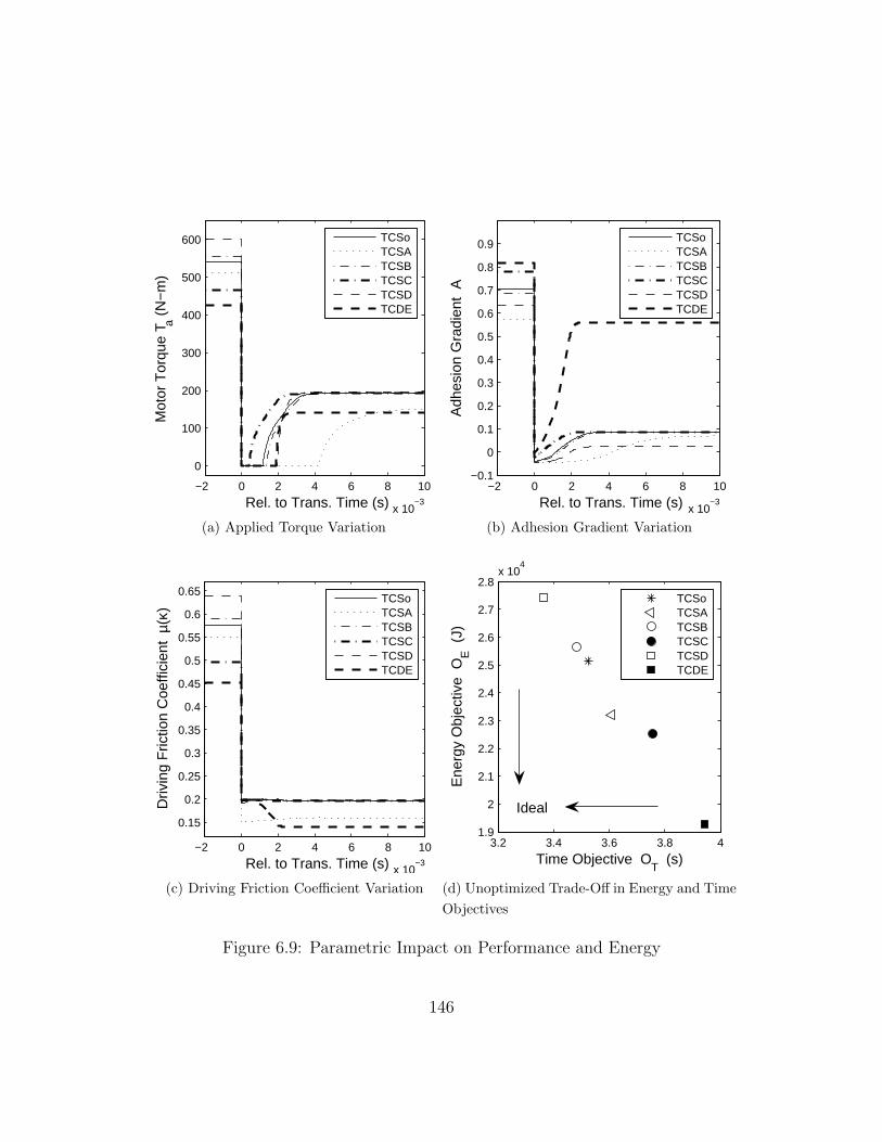
−2 0 2 4 6 8 10
x 10−3
0
100
200
300
400
500
600
Mot
or T
orqu
e T a (
N−
m)
Rel. to Trans. Time (s)
TCSoTCSATCSBTCSCTCSDTCDE
(a) Applied Torque Variation
−2 0 2 4 6 8 10
x 10−3
−0.1
0
0.1
0.2
0.3
0.4
0.5
0.6
0.7
0.8
0.9
Adh
esio
n G
radi
ent
A
Rel. to Trans. Time (s)
TCSoTCSATCSBTCSCTCSDTCDE
(b) Adhesion Gradient Variation
−2 0 2 4 6 8 10
x 10−3
0.15
0.2
0.25
0.3
0.35
0.4
0.45
0.5
0.55
0.6
0.65
Driv
ing
Fric
tion
Coe
ffici
ent
µ(κ)
Rel. to Trans. Time (s)
TCSoTCSATCSBTCSCTCSDTCDE
(c) Driving Friction Coefficient Variation
3.2 3.4 3.6 3.8 41.9
2
2.1
2.2
2.3
2.4
2.5
2.6
2.7
2.8x 10
4
Time Objective OT (s)
Ene
rgy
Obj
ectiv
e O
E (
J)
TCSoTCSATCSBTCSCTCSDTCDE
Ideal
(d) Unoptimized Trade-Off in Energy and Time
Objectives
Figure 6.9: Parametric Impact on Performance and Energy
146

the operation of the traction controller (whose parameters remain unchanged from
TCSo). Torque application Ta in Figure 6.9a is reduced compared to TCSo on both
dry and wet surfaces while the plot of adhesion gradient in Figure 6.9b shows that
Tire 1 is operated closer to its performance limit. This is a result of Tire 1 having
degraded performance compared to Tire 0 and the two figures indicate that Tire 1
operates closer to its limit even when less torque is applied as compared to TCSo.
The performance on wet surface of TCSA is near optimal since adhesion gradient is
small A < 0.1. Therefore the low µ(κ) observed on the wet surface in Figure 6.9c is
due to a limitation in tire force generation characteristics. In contrast, the decrease
in µ(κ) on the dry surface compared to TCSo can be countered by a change in
controller to allow a higher Ta and a decrease in A to improve performance on the
dry surface.
Torque re-application for TCSA is delayed relatively longer than TCSo since,
as shown in Figure 6.9b, the adhesion gradient requires a longer amount of time to
become positive. The delay is further explained by considering the differences of the
adhesion gradient characteristics of the performance tire (Tire 0) and the low rolling
resistance tire (Tire 1) shown in Figure 2.10. On the dry surface, Figure 6.9b shows
that TSCo operates Tire 0 at A ≈ 0.7 while TCSA operates Tire 1 at A ≈ 0.6.
Figure 2.10 therefore shows that, on the dry surface, TCSo operates Tire 0 at a
lower tire slip κ than TCSA with Tire 1. The figure also shows that, on the wet
surface, the optimal slip corresponding to A = 0 is similar for both tire. Therefore,
after the road transition, more time is required for the tire slip of TCSA and Tire
1 to decrease such that A = 0.
Setting the location of A-PS to its lower limit in TCSB results in a system
that considers smaller values of adhesion gradient as Positive-Small in comparison
to TCSo. The impact on the shape of the fuzzy logic control surface is shown
in Figure 6.10a where Ta decreases less in response to initial decreases in A as
compared to the controller of TCSo as shown in Figure 3.16. The control surfaces
differ mostly between adhesion gradients of 0.1 and 0.5. Therefore TCSB results
in marginally less torque reduction on the dry surface compared to TCSo as shown
in Figure 6.9a. The marginally higher Ta leads to marginally higher wheel slip and
147
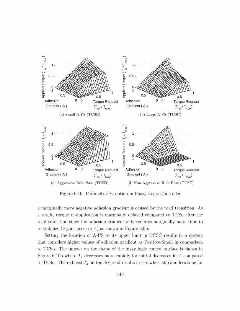
00.5
1
00.5
10
0.5
1
Torque Request (T
ref / T
max)
Adhesion Gradient ( A )
App
lied
Tor
que
( T a /
T max
)
(a) Small A-PS (TCSB)
00.5
1
00.5
10
0.5
1
Torque Request (T
ref / T
max)
Adhesion Gradient ( A )
App
lied
Tor
que
( T a /
T max
)
(b) Large A-PS (TCSC)
00.5
1
00.5
10
0.5
1
Torque Request (T
ref / T
max)
Adhesion Gradient ( A )
App
lied
Tor
que
( T a /
T max
)
(c) Aggressive Rule Base (TCSD)
00.5
1
00.5
10
0.5
1
Torque Request (T
ref / T
max)
Adhesion Gradient ( A )
App
lied
Tor
que
( T a /
T max
)
(d) Non-Aggressive Rule Base (TCSE)
Figure 6.10: Parametric Variation in Fuzzy Logic Controller
a marginally more negative adhesion gradient is caused by the road transition. As
a result, torque re-application is marginally delayed compared to TCSo after the
road transition since the adhesion gradient only requires marginally more time to
re-stabilize (regain positive A) as shown in Figure 6.9b.
Setting the location of A-PS to its upper limit in TCSC results in a system
that considers higher values of adhesion gradient as Positive-Small in comparison
to TCSo. The impact on the shape of the fuzzy logic control surface is shown in
Figure 6.10b where Ta decreases more rapidly for initial decreases in A compared
to TCSo. The reduced Ta on the dry road results in less wheel slip and less time for
148

the wheel to regain stable operation after the road transition. Thus re-application
of Ta occurs sooner than in TCSo and TCSB.
Note. Higher Ta in TCSB translates to higher µ(κ) on the dry road as shown in
Figure 6.9c while the converse is true for lower Ta in TCSC. However, steady-state
performance on the wet road is similar for TCSo, TCSB, and TCSC as shown in
Figure 6.9b and Figure 6.9c. This is due to the choice of the location of the Zero
membership function of the adhesion gradient Z=0.1 and the fact that steady-state
operation of the systems on the wet road occur at A < 0.1. Since membership
in A-PS is zero at adhesion gradients less than Zero, the variation of A-PS does
not affect fuzzy logic controller output on the wet surface. In future research, to
affect steady-state performance on the wet road surface through A-PS, the location
of the Zero membership function could be changed to less than the steady-state
condition to allow non-zero membership in the Positive-Small membership function
of the adhesion gradient. The remaining discussion shows that controller design still
affects operation on both road surfaces through changes in the fuzzy logic rule base.
The aggressive rule base of TCSD results in the least amount of torque reduc-
tion as shown in Figure 6.9a and operates the tire near its limit of performance on
the wet road surface as shown by the low adhesion gradient attained in Figure 6.9b.
Performance on the dry surface is at a maximum since Ta = Tref . Although TCSD
operates the tire at a lower adhesion gradient than TCSo, only a marginal perfor-
mance gain in µ(κ) is obtained on the wet surface as shown in Figure 6.9c. The
definition of C1 - C6 and resulting fuzzy logic control surface of TCSD shown in Fig-
ure 6.10c effectively disable traction control until the adhesion gradient becomes
less than the location of the Zero membership function of the adhesion gradient.
The non-aggressive rule base of TCSE results in the most amount of torque
reduction as shown in Figure 6.9a and does not operate the tire near its limit of
performance as shown by the high adhesion gradient (A > 0.5) on both road surfaces
in Figure 6.9b. As a result, µ(κ) is the lowest in Figure 6.9c. The definition of C1 -
C6 and resulting fuzzy logic control surface of TCSE shown in Figure 6.10d limit
Ta to zero for adhesion gradients less than the location of A-PS = 0.5. Therefore,
the torque re-application after the road transition is delayed in Figure 6.9a until
149

Table 6.6: Percentage of Energy Stored in Vehicle Kinetic Energy
OE vxF ∆Eveh (∆Eveh/OE) × 100
Config. (J) (m/s) (J) (%)
TCSo 25134 8.8396 23142 92.07
TCSA 23202 8.4785 21265 91.65
TCSB 25641 8.9262 23603 92.05
TCSC 22526 8.3760 20747 92.10
TCSD 27423 9.2187 25196 91.88
TCSE 19277 7.7502 17720 91.92
A > 0.5.
The observed trade-offs between energy use and performance listed in Table 6.5
are graphically summarized in Figure 6.9d by plotting OE against OT . The para-
metric study therefore demonstrates that OE and OT are dependent on both plant
and controller design decisions. Further, these system level objectives are depen-
dent on one another and cannot be optimized independently. A necessary trade-off
between OE and OT occurs for variations in system design. As indicated in the
figure, an ideal system would have both low energy use and drive cycle comple-
tion time. Hence an optimization procedure is required to balance energy use and
performance requirements.
Note. As shown in Table 6.6, a significant amount (91-92 %) of drive cycle energy
use OE is stored as kinetic energy ∆Eveh in the moving vehicle. Therefore, the
trade-off between OE and OT is strongly influenced by the final vehicle speed vxF
as obtained by recording vx at time OT such that vxF = vx(OT ). Also, Figure 6.9a
indicates that controller transients persists for less then 10 ms for a drive cycle with
a duration between 3 and 4 seconds (Table 6.5). Therefore, the trade-off between
OE and OT is weakly affected by transient action taken by the controller.
150

Table 6.7: GA Parameters
Parameter Value
Mutation Probability pm 2%
Real-Coded Mutation Standard Deviation σ 0.1
Population Size 200
Terminating Condition After 50 Generations
Number of Parallel CPUs 50
Members per CPU 4
6.4 Simultaneous Optimization Results
The traction control system is optimized with respect to the weighted sum of the
drive cycle energy use OE and completion time OT using the mixed encoding, multi-
chromosomal GA. Problem-independent parameters that impact the execution of
the GA are first described. Results from the simultaneous plant/controller opti-
mization of the traction control system are then analyzed with focus on the impact
of the relative energy to performance weighting on system design. The evolutionary
performance of the GA is examined to further describe its optimization process.
6.4.1 GA Parameters
The numerical values of parameters that affect the operation of the GA are sum-
marized in Table 6.7. The selection of a GA’s parameters is used to balance search
space exploration with running time and influences the quality (optimality) of opti-
mization results. In general, the selection of a GA’s parameters is problem depen-
dent and remains an active area of research with recent advances, for example, in
on-line adaptive tuning of the mutation probability [60]. The following discussion
outlines the parameter selection process applied in this thesis.
The mutation probability is set at pm = 2% in accordance with the general rec-
ommendation that pm < 10% [48] to balance its benefit in generating new building
blocks with its tendency to destroy long building blocks.
151

The standard deviation associated with the Gaussian mutation of the real-coded
variable A-PS is set at σ = 0.1. This allows 99.7% of mutations to produce changes
within 3 standard deviations (±0.3) of A-PS [61]. Therefore, assuming that A-
PS is assigned a nominal value of 0.5, σ = 0.1 generates mutations mostly within
the constrained range of A-PS ∈ [0.2, 0.8] and reduces the probability of repairing
an out-of-bounds mutation.
The population size of 200 and terminating condition of the GA after 50 genera-
tions were chosen based on a trial procedure that results in satisfactory convergence
of the population to a single optimized candidate solution. The evolutionary per-
formance of the GA is further considered in Section 6.4.3.
To achieve a higher fitness evaluation throughput rate, the GA is implemented
using the parallel farmer-worker architecture described in Section 5.1.4. For each
generation, the farmer node selects and distributes 4 sets of parent genetic informa-
tion to 50 worker nodes. For each set of parents received, the worker nodes perform
the crossover and mutation operations to generate a new candidate solution in ad-
dition to objective evaluation through system simulation. The resulting offspring’s
genetic information and simulation results are then sent back to the farmer node
for fitness evaluation and selection for the next generation.
6.4.2 Impact of Energy Use to Performance Weighting
Simultaneous plant/controller optimization results of the traction control system
are summarized in Table 6.8. Six optimization runs, labeled as TCS1 to TCS6, were
performed under different energy weights wE. For each optimization run, the table
lists the individual drive cycle energy use OE and completion time OT objectives
used in the calculation of the system-level objective Os. In addition, the table shows
the resulting optimized assignment of system design variables TIRE, A-PS, and
NODE that specify the selection of vehicle tire, the location of the Positive-Small
adhesion gradient membership function, and the fuzzy logic rule base configuration,
respectively. Finally, the table indicates the level of the selected rule base (from
Figure 5.19). The following discussion describes the selection of the energy weight
wE coefficient and its impact on optimization results. The optimized results are
152

Table 6.8: Optimization Results for Various Energy Weights wE
Config. wE OE OT Os TIRE A-PS NODE level
TCS1 0 27423 3.3638 3.3638 0 0.38005 2 1
TCS2 1e-6 26748 3.3640 3.3908 1 0.26404 1 0
TCS3 8e-6 26718 3.3643 3.5780 1 0.37270 15 3
TCS4 10e-6 26654 3.3648 3.6314 1 0.36856 33 5
TCS5 12e-6 26474 3.3667 3.6844 1 0.40093 53 6
TCS6 100e-6 16621 4.1552 5.8168 1 0.60768 83 11
then compared with the unoptimized nominal system TCSo from Section 6.3.1.
The energy weight coefficient wE controls the relative importance of the energy
objective OE and the time objective OT in the minimization of their weighted sum
Os (4.12). To avoid having one objective dominate the other, a knowledge of the
scalar range of the individual objectives is required to select an appropriate numeri-
cal value for wE. Although Table 6.8 lists the optimization runs by ascending values
of energy weight, the optimizations were performed in a different order beginning
with an initial selection of wE derived from the results of the parametric study sum-
marized in Table 6.5. Consideration of Table 6.5 indicates that OE changes on the
order of 1e2 to 1e4 while OT changes on the order of 1e-1. Hence, an initial energy
weighting of wE = 1e-5 (corresponding to optimized system TCS4) was selected to
approximately balance the optimization of OE and OT . To determine the impact of
objective weight selection on the optimized system, simulation runs were performed
where wE is an order magnitude smaller (TCS2) and larger (TCS6) then used in
TCS4. In comparing the resulting optimized selection of NODE in Table 6.8, it was
noted that a change in an order of magnitude in wE resulted either in the selection
of a very aggressive rule base configuration in TCS2 (level(NODE = 1) = 0) or
a very non-aggressive rule base configuration in TCS6 (level(NODE = 83) = 11).
Therefore, additional optimization runs were performed with wE deviating from
TCS4 by -2e-6 in TCS3 and +2e-6 in TCS5. Since the tire selection TIRE, did not
change in TCS2 to TCS6, an optimization run with wE = 0 in TCS1 was performed
153

to verify the operation of the GA.
Overall, the simulation results in Table 6.8 show the following trends:
• Energy use OE decreases while drive cycle completion time OT increases as the
weighting on energy use is increased. These trends are expected and confirm
the trade-off between energy economy and vehicle performance. Thus, the
selection of wE determines how the optimization process balances conflicting
objectives in the minimization of OE and OT .
• The system-level objective Os increases with wE since OE is four orders of
magnitude larger than OT and therefore increases in wE tend to cause a net
increase in Os. The trend is purely a consequence of the scalar range of
the individual objective functions OE and OT . In general, Os is only used
internally to determine an optimized solution within an optimization run and
does not have significance when compared across optimization runs.
• Optimization runs TCS2 to TCS6 indicate that the use of a low rolling re-
sistance tire (TIRE=1) leads to an optimal system configuration whenever
energy use is considered. In other words, unless performance is the only cri-
teria in the vehicle design with wE = 0 in TCS1, the energy saving benefit
resulting from the use of a low rolling resistance tire outweighs the incurred
degradation in longitudinal tire performance.
• The location of the Positive-Small adhesion gradient membership function A-
PS tends to be greater for larger weightings of energy use (TCS4 to TCS6).
This is expected since a larger value of A-PS causes a quicker decrease in Ta
for initial decrease in A as shown in the comparison of Figure 6.10a and Fig-
ure 6.10b. Therefore, systems with higher values of A-PS tend to output less
torque Ta when operating the tire over similar ranges of A and are associated
with lower OE and higher OT .
The contrary trend observed between TCS3 and TCS4 may indicate that
system objectives may be less sensitive to changes in A-PS than in NODE.
This is partially supported by the results of the parametric study summarized
154

Table 6.9: Impact of A-PS Variation in TCS1 on Objectives
Config. A-PS OE OT
TCS1a 0.2 27423.24 3.363832
TCS1b 0.8 27423.26 3.363834
in Table 6.5 where it is seen that the selection of rule base may exhibit a
greater impact (-23.3%, 11.9%) on the objectives OE and OT , respectively,
than the selection of A-PS (-10%, 6.6%).
The values of A-PS for TCS1 and TCS2 cannot be included in the trend anal-
ysis since their rule base configurations make the optimization insensitive to
changes in A-PS. This is numerically demonstrated for TCS1 in Table 6.9 by
taking the system variable selection of TCS1 (TIRE=0 and NODE=2) and
running two additional individual simulations TCS1a, TCS1b with variation
in A-PS. The table shows that the resulting objective values differ in the sev-
enth significant digit. The numerical difference is insignificant since numerical
solver settings were chosen for convergence to 5 significant figures of accuracy
(Section 6.1). Therefore, for the rule base selection of TCS1, the optimization
is insensitive to changes in A-PS and the TCS1 results in Table 6.8 can be
considered identical to those of TCS1a and TCS1b in Table 6.9.
Detailed examination of the rule base selection in TCS1 and TCS2 reveal
the reason for the insensitivity to variation in A-PS. For TCS1 and TCS2,
the respective rule base selection of NODE = 2 and NODE = 1 is such
that C3 = C4 = 3 = MH and C5 = C6 = 4 = H by mapping ΨRULE (4.8).
In conjunction with Figure 3.15b, a traction controller is therefore defined
that prescribes the same output conclusion over a range of Z to PH adhesion
gradient for a given torque request input in the range MH to H. This is
illustrated by a comparison of the fuzzy logic controller surface plot of TCS1a
(Figure 6.11a) against TCS1b (Figure 6.11b). For torque request inputs above
0.5, the plots are nearly identical due to the definition of C3 to C6. For torque
request inputs less than 0.5, the plots show the impact of changes in A-PS on
155

00.5
1
00.5
10
0.5
1
Torque Request (T
ref / T
max)
Adhesion Gradient ( A )
App
lied
Tor
que
( T a /
T max
)
(a) TCS1a: Small A-PS=0.2
00.5
1
00.5
10
0.5
1
Torque Request (T
ref / T
max)
Adhesion Gradient ( A )
App
lied
Tor
que
( T a /
T max
)
(b) TCS1b: Large A-PS=0.8
Figure 6.11: A-PS Variation in Traction Controller Rule Base of TCS1
the fuzzy logic controller since in this region, the location of A-PS determines
the transition of torque output Ta from Medium-Small (C2 = 2) to Small
(C1 = 1). To emphasize the independence of A-PS in the optimization of
TCS1, the trajectory of Ta along the surface plot is shown in Figure 6.11
for both TCS1a and TCS1b. The two trajectories are nearly identical and
result in similar objective values OE and OT as listed in Table 6.9. Since
the trajectories taken are only influenced by the definitions of C3 to C6 as
described in Section 3.3.3, the preceding analysis applies equally to explain
the independence of A-PS in the optimization of TCS2.
• The level of the optimized rule base increases as wE is increased from TCS2
to TCS6. Since an increase in level is observed along with a decrease in OE
and an increase in OT , the optimization results support the assumption that
a higher level corresponds to a less aggressive rule base as stated in (5.20).
The observation also supports the assumption that the level of a fuzzy logic
rule base is a building block in the encoding of the rule base. The novel
encoding of a fuzzy logic rule base as a member of a poset by delta inclusion
(Section 5.3.3) is therefore shown to be efficient since it manipulates the level
of a rule base directly and acts to preserve level information encoded within
156

Table 6.10: Improvement in Optimized Systems over Benchmark TCSo
Config. wE Os Os,TCSo % Improvement
TCS1 0 3.3638 3.5245 4.56
TCS2 1e-06 3.3908 3.5496 4.47
TCS3 8e-06 3.5780 3.7255 3.96
TCS4 10e-06 3.6314 3.7758 3.82
TCS5 12e-06 3.6844 3.8260 3.70
TCS6 100e-06 5.8168 6.0375 3.66
building blocks.
The observed trend can be extended to include the cursory discrepancy ob-
served in TCS1 by noting that NODE=2 for TCS1 and NODE=1 for TCS2
represent rule base conclusions that differ only in C1. Since the choice of
constant Tref only stimulates rule base conclusions C3 to C6 as described in
Section 3.3.3, the selection of either NODE=2 or NODE=1 produces equiv-
alent simulation results for the chosen drive cycle and do not preferentially
impact the optimization process.
A comparison between the optimization results TCS1 to TCS6 and the bench-
mark nominal system TCSo can be made by calculating the unoptimized system-
level objective Os,TCSo consisting of the weighted average of the unoptimized ob-
jective values OE and OT for TCSo obtained from Table 6.5. In Table 6.10, the
comparison of optimized objective values Os for TCS1 to TCS6 against the un-
optimized objective value Os,TCSo of TCSo indicates that the optimization process
allows an objective value improvement of approximately 4% over the various choices
of energy weights wE.
As stated in Section 4.2.3, the solution to a multi-objective optimization problem
is not unique but is instead represented by a Pareto set of designs for which no
individual objective may be improved without compromising any other objective.
In the current traction control system design, the Pareto set is defined as the set
of all globally-optimal designs over the allowable continuous range of the energy
157

weight wE ∈ [0, 1]. Systems TCS1 through TCS6 represent approximate members
of the Pareto set since a GA optimization does not guarantee a global optimization.
An approximation of the Pareto set is plotted in Figure 6.12a using the optimized
objective values of TCS1 to TCS6. The figure also indicates an approximation of
the Pareto front [62] that is defined by interpolating between members of a Pareto
set. Since it is defined in terms of a Pareto set, the Pareto front in Figure 6.12a
defines a boundary that indicates the limits in the simultaneous minimization of
OE and OT over the variation of weight wE. For example, the unoptimized nominal
system TCSo is plotted in Figure 6.12a and is behind the Pareto front.
Further consideration of Figure 6.12a shows that the optimization results in Ta-
ble 6.8 are not evenly distributed along the Pareto front. More optimization runs
are necessary with energy weights wE ∈ [20e-6, 100e-6] to provide an accurate ap-
proximation of the overall Pareto front. The current simulation results do, however,
allow a relatively accurate approximation of the Pareto front with wE ∈ [0, 12e-6]
as shown by plotting TCS1 to TCS5 in Figure 6.12b.
As a member of a Pareto set, a specific optimized traction control system design
cannot be prescribed without further criteria for specifying the relative weighting
of OE and OT . Such criteria is application specific and needs to be developed in
a greater context, for example, as determined by a study on driver preferences.
Without further guidance on the selection of wE, systems TCS1 to TCS6 can be
considered equally optimal in balancing the energy use to performance trade-off.
6.4.3 Evolutionary Performance of the GA
As a heuristic optimization method, a GA does not guarantee global optimality
although it may be effective at finding near optimal solutions. In general, the fitness
evaluation and selection process of a GA causes diversity in an initial population
to converge towards a fit candidate solution that has been created by the use of
genetic operations. As discussed in Section 6.4.1, the optimality of the final solution
is affected by the selection of a GA’s parameters. The following analysis of the
evolutionary performance of the mixed encoding, multi-chromosomal GA provides
further insight into the influence of the GA’s parameter selection on its optimization
158

3.4 3.6 3.8 4 4.2 4.41.6
1.8
2
2.2
2.4
2.6
2.8x 10
4
Time Objective OT (s)
Ene
rgy
Obj
ectiv
e O
E (
J)
Pareto FrontTCS1TCS2TCS3TCS4TCS5TCS6TCSo
Ideal
(a) Overall Pareto Set Approximation
3.364 3.366 3.368 3.372.64
2.66
2.68
2.7
2.72
2.74
x 104
Time Objective OT (s)
Ene
rgy
Obj
ectiv
e O
E (
J)
Pareto FrontTCS1TCS2TCS3TCS4TCS5
(b) Pareto Set Approximation Detail
Figure 6.12: Approximation of Pareto Set
159

0 10 20 30 40 503.6
3.65
3.7
3.75
3.8
3.85
Generation #
Sys
tem
−Le
vel O
bjec
tive
Os
Best O
s
Pop. Avg. Os
(a) Overall Performance
0 20 403.63134
3.63135
3.63136
3.63137
Generation #
Sys
tem
−Le
vel O
bjec
tive
Os
Best O
s
(b) Convergence Detail
Figure 6.13: Evolutionary Performance of the GA for TCS4
process.
For the GA’s parameters listed in Table 6.7, Figure 6.13 provides a graphical
representation of the GA performance for the TCS4 optimization run. Overall
performance is summarized in Figure 6.13a where the best (minimum) system-
level objective value Os within each generation is plotted over the evolution of the
population (Gen. #). The plot indicates that the GA finds a near optimal solution
within the initial population (Gen. 0) with numerically insignificant improvement
(Figure 6.13b) during the course of the optimization process. The average Os over
all members of each generation is plotted in Figure 6.13a and shows that population
members tend to converge towards the fit candidate solution.
The presence of a near optimal solution within the initial population of a GA
is generally not expected since population size typically limits initial search space
coverage. However, consideration of the discrete portion of the search space spe-
cific to the current traction control system optimization problem reveals that 168
discrete combinations exists as a result of the limited selection from among 84 rule
160

base possibilities and 2 tire selections. Due to the use of a constant Tref that only
stimulates a portion of the rule base as explained in Section 3.3.3, some of the 84
rule base configuration possibilities are equivalent (specifically those with identical
C3 to C6). Since the population size is 200 (from Table 6.7), it is large enough to
more than doubly cover the discrete search space and thus increases the possibility
of a near optimal solution being present in the initial population. It is expected
that a near optimal candidate solution would be absent from the initial population
if the population size is decreased.
Further insight into the operation of the GA is provided by plotting a histogram
(frequency count) of values assumed by optimization variables per generation over
the evolution of the population. Such plots are shown, for the optimization of
TCS4, in Figures 6.14a to 6.14c and depict the distribution of values assumed by
optimization variables TIRE, NODE, and A-PS, respectively. To simplify graphical
interpretation, consecutive nodes numbers are binned in groups of 7 in the distri-
bution of NODE shown Figure 6.14b. Similarly, the distribution of the values of
A-PS in Figure 6.14c is also binned such that each bin represents a range of 0.05.
All three plots show an approximately uniform distribution in the values of the
optimization variables at the initial generation (Gen. 0) caused by random popu-
lation initialization. As new generations are created, the plots show convergence
towards the optimized solution for TCS4 listed in Table 6.8 before the termination
of the optimization process at Gen. 50. For example, Figure 6.14a indicates that
approximately half (100) of the candidate solutions in Gen. 0 select the perfor-
mance tire TIRE=0 while by Gen. 50, all 200 candidate solutions select the low
rolling resistance tire TIRE=1.
Although, Figure 6.13a indicates the presence of the near optimal solution of
TCS4 within the initial population, the plots of the evolution of TIRE and A-
PS show an initial increase, and hence preference, in candidate solutions containing
non-optimal TIRE=0 (up to Gen. 4) as well as A-PS ∈ [0.25, 0.3] (up to Gen.
10). Intuitively, this indicates that a number of good solutions exist with these
characteristics and initially results in a higher combined probability of selection than
the final solution of TCS4. However, the high fitness characteristics associated with
161

10
20
30
40
50
0 10
100200 Gen. #
TIRE
Cou
nt
(a) Evolution of Tire Selection
0
10
20
30
40
50
1 28 56 84
0
100
200
Gen. #
NODE (7 Nodes/Bin)
Cou
nt
(b) Evolution of Rule Base Selection
0
10
20
30
40
50
0.2 0.4 0.6 0.8
0
100
200
Gen. #
A−PS (Binned)
Cou
nt
(c) Evolution of A-PS Selection
Figure 6.14: Optimization Variable Distribution for TCS4
162

the variable selections in TCS4 allow them to spread through the entire population.
Therefore, the reversal of the frequency trends of TIRE and A-PS demonstrate the
expected survival of fit building blocks and supports the general building block
hypothesis of the GA operation stated in Section 5.1.1.
163


Chapter 7
Conclusions and Future Work
A simultaneous plant/controller optimization is performed on an electric vehicle
traction control system with respect to conflicting energy use and performance ob-
jectives. Compared to a typical sequential plant then controller design process, the
formulation of a combined plant/controller design problem enables overall improve-
ment of a system design. Although a highly simplified traction control system is
considered, the resulting optimization problem exhibits characteristics in common
with larger problems including: a coupling between plant and controller design
variables that precludes their independent optimization, a mixture of both contin-
uous and discrete design variables, and the presence of nonlinear system dynamics
requiring simulation to evaluate optimization objectives. The optimization of the
traction control system requires development of a system model, formulation of
the optimization problem, and the proposal, implementation, and execution of a
solution strategy.
The system model consists of a vehicle drive cycle, vehicle model, and traction
controller. A simple drive cycle is used to evaluate the dynamic response, energy
use OE, and completion time OT (representing performance) of a vehicle under a
straight-line acceleration over 20 m. A road transition is located midway in the
drive cycle and is represented by a step change from a dry road to a wet road
with an 80% reduction in coefficient of friction. Vehicle dynamics are described
using a single-wheel longitudinal model to focus analysis on longitudinal tire force
165

generation and rolling resistance.
Longitudinal tire force Fx is a strong function of the tire slip κ ∈ [0, 1] that is
caused by differences in vehicle speed and linear wheel speed. Under free rolling
conditions Fx = 0 and κ = 0. For increasing κ, Fx exhibits an initial increase to a
peak force at an optimal κ∗ before decreasing to a fraction of its maximum at κ = 1.
In general, the position of the peak force, κ∗, and hence the tire performance limit,
change with road conditions. Therefore, the Magic Formula is used to model Fx
generation on the dry road, and the similarity method is used to extrapolate tire
force characteristics on the wet road. Further, tire adhesion gradient A provides an
alternative method of locating optimal κ∗ since it is defined proportionally to the
derivative of Fx and therefore exhibits a positive to negative sign change at κ∗.
Tire rolling resistance is caused by energy loss associated with the cyclic de-
formation experienced by portions of a rolling tire as they contact the ground.
Rolling resistance is modeled as a constant moment opposing wheel rotation. The
observation that rolling resistance decreases as inflation pressure increases allows
the tire force generation characteristics of a low rolling resistance tire to be derived
from those of a highly inflated tire. Compared to the tire force characteristics of
a performance tire (Tire 0), a low rolling resistance tire (Tire 1) exhibits a lower
peak force and its use incurs a trade-off in tire performance to energy economy.
The selection of either Tire 0 or Tire 1 for use in a vehicle design is represented by
the variable TIRE in the overall traction control system optimization.
The quick and accurate torque generation and measurement capabilities in-
herent in an electric vehicle propulsion enables the design of a high performance
traction control system such as the adhesion gradient fuzzy logic controller pro-
posed in [12]. The adhesion gradient traction controller monitors driver torque
request Tref and tire adhesion gradient A and decreases output torque application
Ta to a vehicle wheel when adhesion gradient decreases towards zero. The torque
reduction enables recovery from unstable tire operation where κ → 1 causes ex-
cessive wheel speed, high energy consumption, and decreasing Fx. The adhesion
gradient controller in [12] is adopted in this work. However, in place of a manual
parameter tuning procedure, the non-intuitive specification of the location (shape)
166

of the Positive-Small adhesion gradient membership function A-PS and a portion of
the fuzzy logic rule base RULE is considered in the overall traction control system
optimization.
A traction control system optimization problem is defined in terms of the min-
imization of the weighted sum of OE and OT over the selection of variables TIRE,
A-PS, and RULE. The system model is incorporated within an optimization loop
and the all at once variable selection strategy is implemented using a GA to it-
eratively explore the search space. A mixed-encoding, multi-chromosomal GA is
designed to encode the mixture of continuous and discrete optimization variables
within three single-gene chromosomes of different data types. The variables TIRE,
and A-PS are represented, respectively, using standard encodings for a single bit
binary string, and a real-valued number while a novel fuzzy logic rule base encoding
is developed and applied to indirectly represent RULE.
Attention to rule base encoding is required since the direct encoding of rule base
conclusions as independent integers results in exponential growth of the search
space with the number of rule base entries. A 98% reduction in feasible search
space may be obtained by imposing constraints on rule base entries derived from the
intuitive observation that a rule base should prescribe an increase in Ta as controller
inputs Tref and A increase. Under a direct encoding, the constraints create a
large infeasible search space and introduce computational overhead in handling
infeasible candidate solutions. A novel rule base encoding is therefore proposed
to simultaneously address the challenges in rule base constraint satisfaction and
search space reduction. Possible rule base configurations are defined as nodes and
assigned a level within the novel definition of a partially ordered set (poset) by delta
inclusion. A relationship is assumed between the level of a rule base configuration
and its impact on optimization objectives OE and OT where a high node level is
associated with a low OE and a high OT . The relationship allows the level of a
rule base to be considered as a building block of genetic information that influences
the overall fitness of a candidate solution in a GA. Hence, the rule base RULE is
indirectly represented by a variable NODE that references a corresponding rule base
configuration within a poset by delta inclusion. Specialized crossover and mutation
167

operations are defined on NODE to directly manipulate the level of the referenced
rule base configuration.
Both unoptimized (open loop and closed loop) and optimizing (closed loop)
simulation studies are performed, using the previously described drive cycle, to
allow analysis of the traction control system design. A simulation convergence
study is done to determine numerical solver settings and establish the numerical
accuracy of results to 5 significant figures.
Open loop simulation of the uncontrolled vehicle model shows that constant
torque application leads to unstable tire operation when the road surface transition
causes a reduction in the road surface coefficient of friction. Imposing a prefixed
open loop torque limitation to ensure stability under worst case wet road conditions
enables optimal tire operation on the wet road but unnecessarily limits performance
on the dry road. The simulations show the performance limitations of an open
loop system. Further, analytical derivation of the steady-state and limit conditions
attained during operation of the dry and wet road surfaces, respectively, enables the
verification of a correct implementation of the vehicle and tire dynamic equations.
A benchmark drive cycle response of an unoptimized closed loop system is ob-
tained using the adhesion gradient traction controller with nominal parameter def-
initions from [12]. Comparison of the open loop and closed loop simulation results
show that traction control enables a high (but non-optimal) performance across
both dry and wet road surfaces while avoiding the high energy use associated with
unstable tire operation on the wet surface. A parametric study on the nominal
closed loop system shows that changes in any of the system design variables TIRE,
A-PS, and RULE (or NODE) produce conflicting changes in drive cycle energy use
OE and completion time OT . The parametric study establishes the need for an
optimization procedure to balance the trade-off in OE and OT .
In the simultaneous plant/controller optimization of the traction control system,
the specification of the energy weight coefficient wE controls the relative weighting
of OE and OT . A range of optimized designs are obtained through the variation
of wE across multiple optimization runs. Optimization results indicate that, un-
der straight-line acceleration and unless energy concerns are completely neglected
168

(wE = 0), low rolling resistance tires should be incorporated in a traction control
system design since the energy saving benefits outweigh the associated degradation
in longitudinal tire performance. A weak relationship between an increase in A-
PS and an increase in wE exists since the sensitivity of OE and OT to changes in
A-PS is dependent on rule base configuration. Finally, the level of a selected rule
base configuration is observed to increase with wE. Since wE controls the relative
weighting between OE and OT , an increase in wE causes a decrease in OE and an
increase in OT . Therefore, optimization results support the assumption that a rule
base of high level results in low OE and high OT . Consequently, the novel encoding
of a fuzzy logic rule base as a member of a poset by delta inclusion is shown to be
efficient since its crossover and mutation operators manipulate the level of a rule
base directly.
7.1 Future Work
To facilitate the consideration of the simultaneous plant/controller optimization of
the traction control system, various assumptions are made to simplify both the
system model as well as the optimization process itself. Future work to be consid-
ered can be classified as improvements and extensions to either the traction control
system model, or the optimization process.
The following improvments and extensions relating to the drive cycle, vehicle
and tire model, and adhesion gradient controller should be considered in future
studies of the high performance traction control of low rolling resistance tires:
• Although the simple drive cycle considered in this work enables analysis of
the basic system response to a step change in road friction with constant
driver torque resquest Tref , it restricts controller operation to a single dimen-
sion along a two dimensional surface defined by controller inputs Tref and
adhesion gradient A. Also, the basic system response is dominated by steady
state operation before and after the road transition with a relatively quick
transient behavior at the road transition. A longer drive cycle design incor-
porating varying Tref and more transients in the road surface coefficient of
169
friction should be considered to approximate realistic driving conditions in
the development of a practical traction controller.
• Although an ideal traction control system exhibits both low energy useOE and
completion time OT , it may be more intuitive to formulate an optimization
problem in terms of maximizing energy efficiency and minimizing completion
time. Analysis of the simulation results from the parametric study shows
that 91-92% of energy use is associated with the kinetic energy ∆Eveh used
to accelerate a vehicle. Thus, the use of OE as a minimization objective
implicitly penalizes systems with a high final speed at the end of the drive
cycle. The maximization of system efficiency, defined as ∆Eveh/OE would
allow the optimization of final vehicle speed to be defined separately if desired.
• The use of the single-wheel longitudinal model in the current work neglects
the vertical dynamic weight transfer from front to rear wheels associated with
vehicle acceleration. Since tire force generation and rolling resistance are influ-
enced by normal loading, a longitudinal bicycle model should be implemented
to consider dynamic weight transfer when significant amounts of acceleration
are modeled. Aerodynamic resistance should also be modeled since the as-
sociated vehicle speed-dependent drag force contributes to dynamic weight
transfer.
• The longitudinal tire force generation model may be refined by modeling the
impact of normal loading on tire deformation and distinguishing between the
effective rolling radius re and loaded tire radius r. In general, the two radii are
nonlinear functions of tire wear, vertical loading, and speed [23]. The effective
rolling radius is used in the calculation of wheel slip κ while the loaded radius
determines the moment countering wheel rotation caused by tire force Fx.
Also, a singularity exists in the definition of tire slip that prevents describing
tire operation from a standstill. This may be remedied by defining tire slip
using a differential equation as proposed in [23]; however, the definition in-
troduces new tire dynamics without consideration of their impact on rolling
resistance.
170

• The modeling of tire rolling resistance as a constant neglects its dependence
on tire vertical loading, speed of travel, inflation pressure, and temperature.
Rolling resistance increases proportionally with vertical loading while rela-
tively recent work in [29] describes the dynamic changes in rolling resistance
associated with wheel speed, temperature, and pressure. Studies should be
conducted to determine the relevance of rolling resistance transients in the
design of an energy efficient traction control system.
• The adhesion gradient of a tire cannot be directly measured as assumed in
this work. Therefore, the design of a practical adhesion gradient controller
should include the design of an adhesion gradient observer as proposed in [12].
• Since an adhesion gradient controller does not rely on a tire specific model,
it cannot operate a tire at optimal κ∗ where A = 0. The application of a
corresponding torque Ta at A = 0 would require a calculation involving a tire
force generation model. Future work may investigate the use of an integral
controller in conjunction with an adhesion gradient controller to gradually
increase Ta beyond those prescribed by the adhesion gradient controller and
up to the amount Tref requested by the driver while A > 0.
• The vehicle and tire models may be extended to allow system optimization
with respect to cornering maneuvers. It is an open area of research to consider
the modeling of tire rolling resistance during cornering maneuvers.
• Ultimately, experimental results should be used to validate simulations of the
traction control system model. Initial experiments may involve the use of an
external, rotational-loading motor to emulate tire force generation character-
istics as proposed in [12] and [13]. Experiments may then progress towards
in-vehicle testing similar to those in [10].
The following consideration of future work related to rule base encoding, Pareto
front optimization, automated GA parameter control, and plant/controller design
coupling pertain to the improvement and extension of the proposed simultaneous
plant/controller optimization process:
171

• Currently, the specialized crossover and mutation operations of the novel
encoding of the fuzzy logic rule base depend on a precomputed Hasse diagram
that indicates the relationship of members within a poset by delta inclusion.
A potential weakness exists in the storage requirements for the Hasse digram
since the unconstrained search space size increases exponentially with the
number of rule base entries. It is proposed to investigate the derivation of
an analytical expression to calculate the number of members within a poset
by delta inclusion to determine its space complexity. Such an expression may
also support the decision to redesign the crossover and mutation operations
to dynamically compute required portions of the Hasse diagram to minimize
memory requirements.
• An open research problem exists in the encoding and definition of genetic
operations that permit the minimization of the number of rules in a rule
base. The challenge lies in determining suitable building blocks that may be
preserved during the crossover between, and mutation to, matrices of different
sizes.
• Multiple simulation runs are used in the current work to produce a variety
of optimized traction control systems corresponding to different weightings in
energy use and performance objectives. These systems approximate a Pareto
set and their analysis reveals limitations in system design. Thus, determina-
tion of a Pareto set of a multi-objective optimization problem provides valu-
able design guidance. Rather than generating a Pareto set through repeated
execution of the GA by manually choosing different weightings between ob-
jectives, it is proposed to consider a non-aggregating approach that directly
considers the optimization of multiple objectives. This may be achieved, for
example, by modifying the selection routine to create a Niched Pareto GA to
spread population members along the Pareto frontier in a single optimization
run as described in [63].
• Due to the relatively small size of the optimization problem considered in
this work, the GA parameters including mutation rate, population size, and
172

number of generation before termination are chosen using a trial procedure
to allow a satisfactory exploration of the search space. In general, the com-
putational requirements required to optimize a larger problem may preclude
the convenience of executing trial optimization runs for the purpose of man-
ually tuning the GA parameters. For such problems, the incorporation of
automated, dynamic control of the GA parameters during the GA execution
is recommended. An overview of parameter control mechanisms is provided
in [64].
• Only a partial coupling between plant and controller design variables exists
in this work since the traction controller design does not impose constraints
on the vehicle design. In general, a full coupling loop exhibiting mutual
dependence between plant and controller variables is expected in a simulta-
neous design problem. In contrast to the ideal concurrent variable selection
strategy, the all at once strategy allows a relaxation in either the plant to con-
troller constraints or the controller to plant constraints to facilitate system
optimization. Implementation of a penalty scheme within the GA is rec-
ommended to minimize deviation from the optimal condition with coupling
constraint equality. The traction control system optimization problem may
be extended to introduce a full coupling loop by incorporating a motor design
as demonstrated in [17] where the specification of minimum motor power is
derived from dynamic controller performance and controller performance is
in turn dependent on the armature resistance and inductance derived from a
motor design.
173


Appendix A
Traction Control System
Parameters
Tables A.1 to A.4 list the numerical values used in the model of the traction control
system.
Table A.1: Single-Wheel Vehicle Parameters
Component Parameter Value Source(1)
Vehicle Mass m = 600 kg [23]
Wheel Inertia Jw = 1 kg m2 [23]
Wheel Radius r = 0.3 m [23]
Initial Velocity vxo = 1 m/s -
Initial Wheel Speed Ωo = vxo/r -
175

Table A.2: Drive Cycle Parameters
Component Parameter Value Source(1)
Road Transition Distance ST = 10 m -
Final Distance SF = 20 m -
Torque Reference Tref = 600 N m -
Maximum Torque Tmax = 720 N m -
Dry Friction µdry = 1.0 -
Wet Friction µwet = 0.2 -
Table A.3: Tire Parameters
Component Parameter Value Source(1)
Tire Shape Factor Cx = 1.6 [23]
(Common) Curvature Factor Ex = 0 [23]
Nominal Load Fzo = 3000 N -
Tire 0 Stiffness Factor Bxo = 12.5 [23]
(Performance) Peak Factor Dxo = 3000 N [23]
Rolling Resistance Coefficient Cr = 0.014 [22]
Tire 1 Stiffness Factor Bxo = 9.375 -
(Low Rolling Peak Factor Dxo = 2400 N -
Resistance) Rolling Resistance Coefficient Cr = 0.007 [22]
176
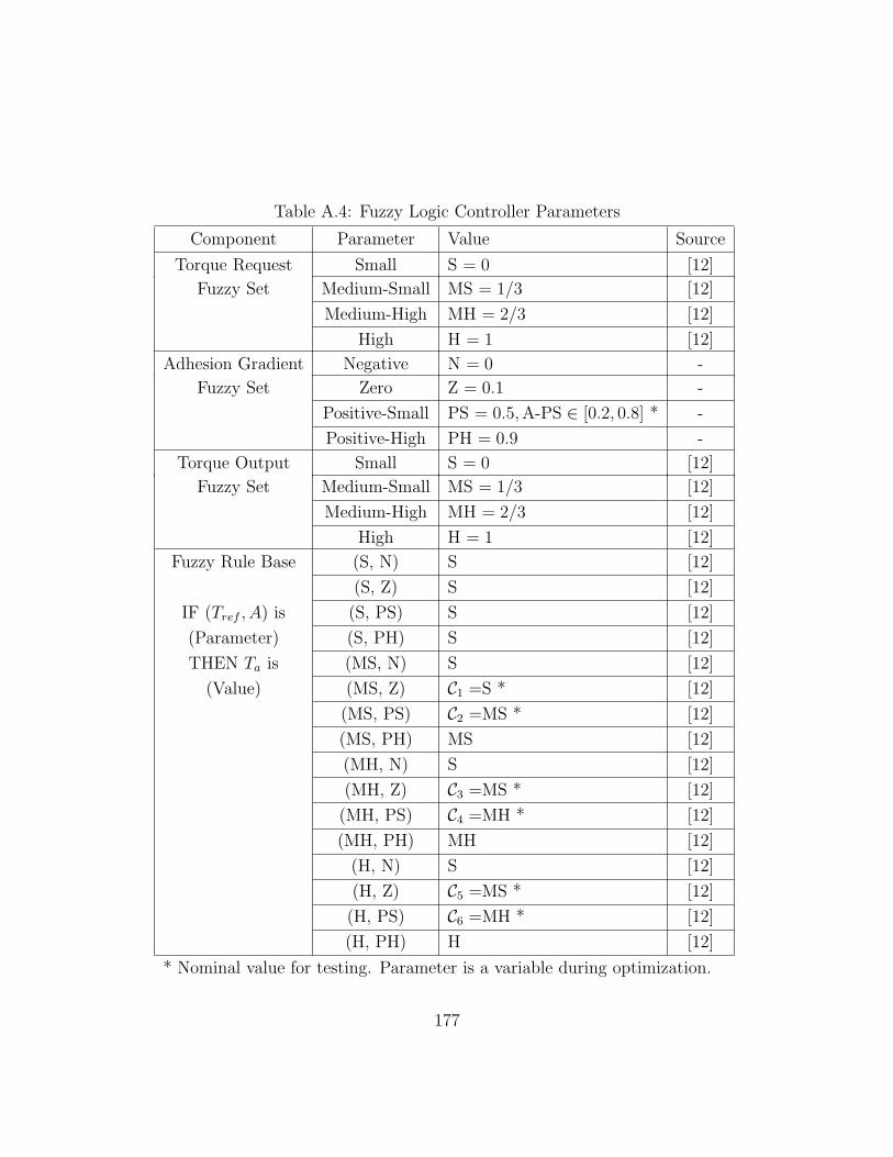
Table A.4: Fuzzy Logic Controller Parameters
Component Parameter Value Source
Torque Request Small S = 0 [12]
Fuzzy Set Medium-Small MS = 1/3 [12]
Medium-High MH = 2/3 [12]
High H = 1 [12]
Adhesion Gradient Negative N = 0 -
Fuzzy Set Zero Z = 0.1 -
Positive-Small PS = 0.5,A-PS ∈ [0.2, 0.8] * -
Positive-High PH = 0.9 -
Torque Output Small S = 0 [12]
Fuzzy Set Medium-Small MS = 1/3 [12]
Medium-High MH = 2/3 [12]
High H = 1 [12]
Fuzzy Rule Base (S, N) S [12]
(S, Z) S [12]
IF (Tref , A) is (S, PS) S [12]
(Parameter) (S, PH) S [12]
THEN Ta is (MS, N) S [12]
(Value) (MS, Z) C1 =S * [12]
(MS, PS) C2 =MS * [12]
(MS, PH) MS [12]
(MH, N) S [12]
(MH, Z) C3 =MS * [12]
(MH, PS) C4 =MH * [12]
(MH, PH) MH [12]
(H, N) S [12]
(H, Z) C5 =MS * [12]
(H, PS) C6 =MH * [12]
(H, PH) H [12]
* Nominal value for testing. Parameter is a variable during optimization.
177


Appendix B
Longitudinal Bicycle Model
Analysis of a longitudinal bicycle model provides insight into the dynamic weight
transfer between front and rear tires associated with vehicle acceleration. The
analysis is used to derive conditions on vehicle design parameters and operation
that enable the assumption of negligible weight transfer between tires.
Longitudinal and vertical vehicle forces are considered in a planar longitudinal
bicycle model (Figure B.1) to determine the impact of vehicle acceleration on
vertical weight distribution between tires. The vehicle is modeled as a rigid body
with mass m, center of gravity located a distance h above a horizontal road, front
and rear tire-road contact points located at distances l1 and l2, respectively, from
the center of gravity, and wheelbase l = l1 + l2. Half of the physical vehicle mass is
h
Fx1Fx2Fz1Fz2
Fg
FL
l1l2
l
Figure B.1: Longitudinal Bicycle Model During Braking [23]
179

modeled in m to account for the fact that half of the wheels are modeled.
Front and rear normal forces Fz1 and Fz2, respectively, are present at the tire-
road contact points in reaction to gravitational force:
Fg = mg = Fz1 + Fz2 (B.1)
where g ≈ 9.81 m/s2 is the gravitational constant. Front and rear longitudinal tire
forces Fx1 and Fx2, respectively, arise due to longitudinal reaction forces produced
by the road on the tires as a result of propulsion or braking action. The direction
of the longitudinal forces is positive (points forward) during propulsion and nega-
tive (points backwards) during braking. In Figure B.1, the longitudinal forces have
been indicated for braking. Though tire force generation mechanics (such as wheel
rotation and tire deformation) are not explicitly modeled, the maximum longitu-
dinal force available from each tire can still be determined if it is assumed that it
is friction-limited by the amount of normal force exerted on the tire (as is the case
with powerful propulsion and braking systems). For a road with uniform coefficient
of friction µ, the longitudinal and normal tire forces are related as follows:
|Fx1| ≤ |Fx1max| = µFz1 |Fx2| ≤ |Fx2max| = µFz2 (B.2)
Analysis of the longitudinal bicycle model provides the following insight on the
limits of vehicle and tire longitudinal performance:
• Vehicle longitudinal acceleration is limited by surface friction. The vehicle
acceleration a is determined by Newton’s second law:
a =Fx
m(B.3)
where Fx = Fx1 + Fx2 is the net external longitudinal force applied by road
on the front and rear tires.
However, the longitudinal force Fx acting on the vehicle is limited by (B.2)
since it is the sum of friction-limited longitudinal tire forces:
|Fx| ≤ |Fx1max| + |Fx2max| = µ(Fz1 + Fz2) = µFg. (B.4)
180

Therefore, by substitution of (B.1) and (B.3) into (B.4), vehicle acceleration
is limited to:
|a| ≤ µ g. (B.5)
Hence, assuming negligible aerodynamic drag and downforce [65], maximum
vehicle acceleration is limited by the gravitational constant and the coefficient
of friction µ between tire and road.
• Longitudinal tire forces Fx1 and Fx2 are limited by dynamic variation of nor-
mal forces as a function of vehicle longitudinal acceleration. Tire normal
forces may be analyzed by applying d’Alembert’s Principle [66] to convert
the vehicle longitudinal dynamics in (B.3) into a static system by reformulat-
ing Newton’s second law:
Fx = ma ↔ Fx + FL = 0 (B.6)
where FL = −ma is a fictitious inertial force acting longitudinally on the
vehicle center of gravity in the opposite direction of vehicle acceleration as
indicated in Figure B.1.
Tire normal forces are calculated by considering the sum of moments produced
by gravitational, inertial, and normal forces about the rear and front tire-road
contact points for the front and rear tires, respectively:
Fz1 = Fg
l − l1l
+FL × h
l(B.7a)
Fz2 = Fg
l1l︸ ︷︷ ︸
static
−FL × h
l︸ ︷︷ ︸dynamic
. (B.7b)
The first terms of both (B.7a) and (B.7b) represent the contribution to normal
force as a result of static weight distribution determined by the longitudinal
location of the vehicle center of gravity. The second terms represent the
contribution to normal force caused by dynamic weight transfer resulting
from vehicle acceleration and deceleration. Although the individual front and
rear tire normal forces vary, the total normal force remains in balance with
181

gravitational force (as seen by substituting (B.7) into (B.1)). Therefore the
limits of longitudinal tire performance in (B.2) are dynamic and vary with
vehicle acceleration as described by (B.7).
By assuming a low center of gravity (small h), long wheel base (large l), and low-
to-moderate accelerations (small FL), the dynamic weight transfer terms in (B.7)
can be neglected. Therefore, the normal forces acting on a tire are determined
solely by the static weight distribution terms in (B.7) and the assumptions allow
longitudinal tire performance to be considered independently of vehicle acceleration.
182

Appendix C
Tire Operating Conditions
Additional background on general tire operating conditions and associated forces
and moments is provided to establish a basis for future consideration of a vehicle
model incorporating dynamics due to vehicle acceleration and cornering maneuvers.
In general, the operating conditions, forces, and moments of a tire may be
described using the coordinate system and parameters shown in Figure C.1. The
road surface is defined relative to a fixed inertial reference coordinate system at
point O. The position of the center of the wheel is defined by point A relative to
point O. At a radial distance r from A, the tire is in contact with an area of the
road surface called the contact patch. All forces and moments required to move a
vehicle are generated within the contact patch and assumed to act on the contact
center at point C [23]. The road surface near the contact patch is approximated
by a flat ground plane with normal vector n pointing upwards. The wheel rotates
about a wheel axle s with angular speed Ω. The wheel rotation occurs within a
wheel center plane passing through the wheel center A and the contact center C
and perpendicular to the wheel axle s.
The orientation of the wheel is defined relative to a local coordinate system at
point C on the road surface. The x-axis points forward along the line of intersection
between the ground plane and the wheel center plane. The y-axis points right along
the ground plane perpendicular to the x-axis. The z-axis points downwards normal
to the ground plane (−n). The wheel velocity, and hence the velocity vC of the
183

Inertial
Reference O
C
Ground Plane
Wheel Centre PlaneNormal to
Ground Plane
A
Wheel Axle
r
n
s
x
y
z
vC
Ω
γ
α
Fz
Fy
Fx
Tz
Ty
Tx
Figure C.1: Position, Motion, Forces, and Moments for Road and Tire [23]
contact center may differ from the direction in which the tire is pointed by a slip
angle α from the x-axis. The wheel center plane may exhibit a camber angle
γ, relative to the ground plane normal n. Longitudinal, lateral, and normal forces
(Fx, Fy, Fz), and overturning, rolling resistance, and aligning moments (Tx, Ty, Tz)
are defined relative the x, y, and z axes, respectively. The positive direction of
the forces and moments are defined according to right hand convention with the
exception of the vertical force Fz that acts in the same direction as the ground
plane normal n.
Note. Sign conventions in the literature are not uniform and may be chosen, for
example, to minimize the number of negative quantities in a specific application
[23]. The sign convention presented in Figure C.1 is an adapted form of the Society
of Automotive Engineers (SAE) convention and differs in the definition of positive
side slip angle α. Other conventions, such as taken by the International Standards
Organization (ISO), orient the wheel coordinate system such that the (x, y, z) axes
184

Table C.1: Tire Operating Modes [23]
In-Plane Mode Out-of-Plane Mode
(Negligible α, γ, (Constant Ω, vx,
Variable Ω, vx) Variable α, γ)
Primary function Braking/Driving (Fx) Cornering Side Force (Fy)
Load Carrying (Fz)
Secondary effect Rolling Resistance (Ty) Overturning Moment (Tx)
Aligning Moment (Tz)
point forward, left, and upwards, respectively [23].
The definition of the wheel center plane allows a distinction between in-plane,
out-of-plane operating modes of a tire [23]. The two modes of operation are sum-
marized in Table C.1. In the case of straight-line driving or braking, tire camber γ
and slip angle α are assumed negligible and analysis may focus on the generation
of in-plane longitudinal force Fx, normal force Fz, and rolling resistance moment
Ty. In the case of simple cornering maneuvers, the wheel rotational speed Ω and
the forward speed vx (the x-component of the contact center velocity vC) are as-
sumed constant and analysis may focus on the generation of out-of-plane lateral
force Fy, overturning moment Tx, and aligning moment Tz. For complex, and gen-
eral, situations such as braking in a turn, a nonlinear combination of in-plane and
out-of-plane tire operating modes results [23].
Table C.1 also shows that a distinction can be made between the primary func-
tions and secondary (but often important) effects in the operation of a tire [23].
The primary functions of a tire are to transmit forces from the road to a vehicle in
the three perpendicular directions (Fx, Fy, Fz) to affect vehicle speed and direction
while absorbing road irregularities, respectively. Secondary moments (Tx, Ty, Tz)
arise due to large slip angles inducing vehicle roll-over, energy lost in tire deforma-
tion, and uneven lateral force distribution within the contact patch area creating a
moment about the contact center, respectively [23].
185


Appendix D
Simulation Convergence Data
Table D.1 lists the results of simulation convergence tests to determine solver set-
tings in Matlab and Octave using a closed loop traction control system configured
with a performance oriented tire and nominal traction controller parameters.
Solver settings are listed in the maximum step, relative tolerance, and absolute
tolerance columns. Wall clock time is the actual time taken to run a 10 second
simulation of the system on an AMD Sempron 1.60 GHz (Matlab) and on an AMD
Opteron 2.20 GHz node available on SHARCNET (Octave). Data in the energy and
time objective columns represent state variables of the system under consideration
and are affected by solver settings.
187

Table D.1: Numerical Solver Convergence Data
Solver Max. Rel. Abs. Wall Energy Time
Step Tol. Tol. Clock (s) Objective (J) Objective (s)
Matlab R2006a Stiff Solver
ode15s 1e-1 1e-4 1e-4 0.56 25139.86 3.525445
ode15s 1e-1 1e-5 1e-5 0.69 25134.68 3.524545
ode15s* 1e-1 1e-6 1e-6 0.84 25134.17 3.524456
ode15s 1e-1 1e-7 1e-7 1.02 25134.08 3.524441
ode15s 1e-1 1e-8 1e-8 1.26 25134.09 3.524441
Octave 2.1.73 Stiff Solver
lsode 1e-1 1e-4 1e-4 1.23 25135.63 3.524222
lsode 1e-1 1e-5 1e-5 1.67 25133.90 3.524351
lsode* 1e-1 1e-6 1e-6 2.17 25134.08 3.524431
lsode 1e-1 1e-7 1e-7 2.45 25134.09 3.524441
lsode 1e-1 1e-8 1e-8 3.24 25134.09 3.524441
*Selected solver settings
188

Appendix E
Steady State and Limit Condition
Calculations
The following Maple 9.5 code listing is used to calculate steady-state and limit op-
erating conditions of the open loop control of tire and vehicle dynamics. Numerical
results are discussed in Section 6.2.
> restart;> Common:=Cx=1.6, Fzo=3000, r=0.3, m=600, J=1;
> TireA:= Bxo = 12.5, Cx = 1.6, Dxo = 3000, Cr=0.014, Common;> ur_uo_dry:=1; ur_uo_wet:=0.2;> Fx := ur_uo * Dxo * sin(Cx*arctan(Bxo*k/ur_uo));> muk := Fx/Fzo;> Ty := r*Cr*Fzo;
> A := diff(Fx,k) / (Bxo*Cx*Dxo);
189

Common := Cx = 1.6, Fzo = 3000, r = 0.3, m = 600, J = 1
TireA := Bxo = 12.5, Cx = 1.6, Dxo = 3000, Cr = 0.014,
Cx = 1.6, Fzo = 3000, r = 0.3, m = 600, J = 1
ur uo dry := 1
ur uo wet := 0.2
Fx := ur uo Dxo sin(Cx arctan
(Bxo kur uo
))
muk := ur uo Dxo sin(Cx arctan
(Bxo kur uo
))Fzo−1
Ty := rCr Fzo
A := cos(Cx arctan
(Bxo kur uo
)) (1 + Bxo
2k2
ur uo2
)−1
> ss := r*(1-k)*(Ta-Ty-r*Fx)/J = Fx/m;
ss := r (1 − k)(Ta − rCr Fzo − rur uo Dxo sin
(Cx arctan
(Bxo kur uo
)))J−1
= ur uo Dxo sin(Cx arctan
(Bxo kur uo
))m−1
> Ta_nTCSu:=600;
> k_dryss:=fsolve(subs(Ta=Ta_nTCSu, ur_uo=ur_uo_dry, TireA, ss),k);
Ta nTCSu := 600
k dryss := 0.03711144962> Fx_dryss:=evalf(subs(k=k_dryss, ur_uo=ur_uo_dry, TireA, Fx));
> muk_dryss:=evalf(subs(k=k_dryss, ur_uo=ur_uo_dry, TireA, muk));> A_dryss:=evalf(subs(k=k_dryss, ur_uo=ur_uo_dry, TireA, A));
Fx dryss := 1921.053802
muk dryss := 0.6403512675
A dryss := 0.6320640207> muk_wetlim:=evalf(subs(k=1, ur_uo=ur_uo_wet, TireA, muk));> A_wetss:=evalf(subs(k=1, ur_uo=ur_uo_wet, TireA, A));
muk wetlim := 0.1216598993
A wetss := −0.0002031371373
190

Bibliography
[1] Intergovernmental Panel on Climate Change. Climate Change 2001: Synthesis
Report. Cambridge University Press, Cambridge, UK, 2001. [Online]. Avail-
able: http://www.grida.no/climate/ipcc_tar, Oct. 2006 [date accessed].
[2] World Energy Outlook: 2004 Edition. International Energy Agency, Paris
Cedex, France, 2004. [Online]. Available: http://www.iea.org/, Oct. 2006
[date accessed].
[3] International Energy Agency. Key world energy statistics: 2006 edition, 2006.
[Online]. Available: http://www.iea.org, Oct. 2006 [date accessed].
[4] Intergovernmental Panel on Climate Change. Climate Change 2001: The Sci-
entific Basis. Cambridge University Press, Cambridge, UK, 2001. [Online].
Available: http://www.grida.no/climate/ipcc_tar/, Oct. 2006 [date ac-
cessed].
[5] International Energy Outlook: 2006. Energy Information Administra-
tion, U.S. DOE, Washington, DC, June 2006. [Online]. Available:
http://www.eia.doe.gov/oiaf/ieo/, Oct. 2006 [date accessed].
[6] M. Montazeri-Gh and M. Asadi. 2006-01-3293: Influence of the road grade
on the optimization of fuzzy-based hybrid electric vehicle control strategy. In
Powertrain & Fluid Systems Conference & Exhibition, Oct. 16-19, 2006.
191

[7] O. Volpato, F. Theunissen, and R. Mazara. 2005-01-3777: Engine control
module for flex fuel plus compressed natural gas vehicles. In Powertrain &
Fluid Systems Conference and Exhibition. SAE, Oct. 24-27, 2005.
[8] N. Brinkman, M. Wang, T. Weber, and T. Darlington. GM Study: Well-
to-Wheels Analysis of Advanced Fuel/Vehicle Systems - A North Ameri-
can Study of Energy Use, Greenhouse Gas Emissions, and Criteria Pollu-
tant Emissions. Argonne National Laboratory, 2005. [Online]. Available:
http://www.transportation.anl.gov/pdfs/TA/339.pdf, Oct. 2006 [date
accessed].
[9] C. C. Chan and Y. S. Wong. The state of the art of electric vehicles technology.
In The 4th International Power Electronics and Motion Control Conference,
2004. IPEMC 2004., pages 46–57, 14-16 Aug. 2004.
[10] X. Liu, L. Li, Y. Hori, T. Akiba, and R. Shirato. Optimal traction control for
EV utilizing fast torque response of electric motor. In Industrial Electronics
Society, 2005. IECON 2005. 32nd Annual Conference of IEEE, pages 2614–
2619, Nov. 6-10 2005.
[11] Y. Hori. Future vehicle driven by electricity and control-research on four-wheel-
motored “UOT Electric March II”. Industrial Electronics, IEEE Transactions
on, 51(5):954–962, Oct. 2004.
[12] V. Delli Colli, G. Tomassi, and M. Scarano. “Single wheel” longitudinal trac-
tion control for electric vehicles. Power Electronics, IEEE Transactions on,
21(3):799–808, May 2006.
[13] P. Khatun, C. M. Bingham, N. Schofield, and P. H. Mellor. Application of
fuzzy control algorithms for electric vehicle antilock braking/traction control
systems. Vehicular Technology, IEEE Transactions on, 52(5):1356–1364, Sept.
2003.
[14] N. Shidore and M. Pasquier. 2005-01-3457: Interdependence of system control
component sizing for a hydrogen-fueled hybrid vehicle. In Future Transporta-
192

tion Technology Conference, Warrendale, PA, Sept 7-9 2005. SAE Interna-
tional.
[15] S. Golbuff. 2007-01-1545: Design optimization of a plug-in hybrid electric
vehicle. In 2007 World Congress, Warrendale, PA, April 16-19, 2007. SAE
International.
[16] G. L. Ohl, M. J. Prucka, F. S. Kanafani, M. J. Duty, E. DiValentin, and
D. M. Kramer. 2004-01-0893: Development of powertrain coordination at
DaimlerChrysler Corporation. In 2004 SAE World Congress, Warrendale, PA,
March 8-11, 2004. SAE International.
[17] J. A. Reyer and P. Y. Papalambros. Combined optimal design and control with
application to an electric DC motor. Journal of Mechanical Design, Transac-
tions of the ASME, 124(2):183–191, June 2002.
[18] Y. He and J. McPhee. A design methodology for mechatronic vehicles: Ap-
plication of multidisciplinary optimization, multibody dynamics and genetic
algorithms. Vehicle System Dynamics, 43(10):697–733, October, 2005.
[19] W. Wang and J. J. Moskwa. 1999-01-0977: A study on automatic transmission
system optimization using a HMMWV dynamic powertrain system model. In
International Congress and Exposition, Warrendale, PA, March 1-4, 1999. SAE
International.
[20] U. Kiencke and L. Nielsen. Automotive Control Systems: For Engine, Drive-
line, and Vehicle. Springer-Verlag Berlin Heidelberg, New York, 2000.
[21] S. Hegazy, H. Rahnejat, and K. Hussain. Multi-body dynamics in full-vehicle
handling analysis under transient manoeuvre. Vehicle System Dynamics,
34(1):1–24, July 2000.
[22] Tires and Passenger Vehicle Fuel Economy: Informing Consumers, Improving
Performance, volume Special Report #286. Transportation Research Board,
193

National Research Council, Washington, D.C., July 11, 2006. [Online]. Avail-
able: http://www.trb.org/publications/sr/sr286.pdf, Sept. 2006 [date
accessed].
[23] H. B. Pacejka. Tire and Vehicle Dynamics. SAE International, Warrendale,
PA, U.S.A., 2006.
[24] A. Eichberger and M. Schittenhelm. Implementations, applications and
limits of tyre models in multibody simulation. Vehicle System Dynamics,
43(Suppl):18–29, 2005.
[25] Tire Performance Technology - SAE J2047 Feb98, volume 2 of 2002 SAE
Handbook, pages 30.01–30.24. SAE, Warrendale, PA, U.S.A., 2002.
[26] M. Lebel. 1999-01-0788: Multiple applications, multiple roles: How carbon
black technologies help tires roll better. In SAE International Congress and
Exposition, Warrendale, Pennsylvania, USA, March 1-4, 1999. SAE Interna-
tional.
[27] Stepwise Coastdown Methodology for Measuring Tire Rolling Resistance - SAE
J2452 JUN99, volume 2 of 2002 SAE Handbook, pages 30.36–30.57. SAE,
Warrendale, PA, U.S.A., 2002.
[28] P. S. Grover. 980251: Modeling of rolling resistance test data. In SAE Interna-
tional Congress and Exposition, Warrendale, Pennsylvania, USA, Feb. 23-26,
1998. SAE International.
[29] L. Nielsen and T. Sandberg. 2002-01-1200: A new model for rolling resistance
of pneumatic tires. In SAE 2002 World Congress, Warrendale, Pennsylvania,
USA, Mar. 4-7, 2002. SAE International.
[30] P. S. Grover and S. H. Bordelon. 1999-01-0787: New parameters for com-
paring tire rolling resistance. In SAE International Congress and Exposition,
Warrendale, Pennsylvania, USA, March 1-4, 1999. SAE International.
194

[31] Rolling Resistance Measurement Procedure for Passenger Car, Light Truck,
and Highway Truck and Bus Tires - SAE J1269 SEP00, volume 2 of 2002
SAE Handbook, pages 30.57–30.61. SAE, Warrendale, PA, U.S.A., 2002.
[32] J. Y. Wong. Mechanics of Pneumatic Tires, chapter 1, pages 14–15. Theory
of Ground Vehicles. John Wiley, New York, 3 edition, Mar. 2001.
[33] California Energy Commission. California State Fuel-Efficient
Tire Program: Volume I - Summary of Findings and Recommen-
dations. Number Sept 23,. Jan. 31, 2003. [Online]. Available:
http://www.energy.ca.gov/reports/2003-01-31_600-03-001F-VOL1.PDF,
Sept. 2006 [date accessed].
[34] A. J. C. Schmeitz, I. J. M. Besselink, J. De Hoogh, and H. Nijmeijer.
Extending the Magic Formula and SWIFT tyre models for inflation pres-
sure changes. VDI Berichte, (1912):201–225, 2005. [Online]. Available:
http://www.mate.tue.nl/mate/pdfs/5852.pdf, Apr. 2007 [date accessed].
[35] R. Pusca, Y. Ait-Amirat, A. Berthon, and J. M Kauffmann. Fuzzy-logic-based
control applied to a hybrid electric vehicle with four separate wheel drives. In
IEE Proceedings: Control Theory and Applications, volume 151, pages 73–82,
January, 2004.
[36] A. Mirzaei, M. Moallem, B. M. Dehkordi, and B. Fahimi. Design of an optimal
fuzzy controller for antilock braking systems. Vehicular Technology, IEEE
Transactions on, 55(6):1725–1730, Nov. 2006.
[37] K. Furukawa and Y. Hori. Recent development of road condition estimation
techniques for electric vehicle and their experimental evaluation using the test
EV “UOT March I and II”. In Industrial Electronics Society, 2003. IECON
’03. The 29th Annual Conference of the IEEE, volume 1, pages 925–930, Nov.
2-6 2003.
[38] T. J. Ross. Fuzzy Logic: With Engineering Applications. John Wiley & Sons,
Ltd., West Sussex, England, 2004.
195

[39] F. Jinzhi, Y. Fan, and L. Jun. 2002-01-0983: An investigation to controller
design for active vehicle suspension by using GA-based PID and fuzzy logic.
In SAE 2002 World Congress, Mar. 4-7, 2002.
[40] D. Peng, C. L. Yin, and J. W. Zhang. 2006-01-3583: Advanced braking control
system for hybrid electric vehicle using fuzzy control logic. In Commercial
Vehicle Engineering Congress and Exhibition, Oct. 31-Nov. 2, 2006.
[41] M. Davoudi, M. B. Menhaj, and M. Davoudi. 2006-01-3483: A fuzzy based
vehicle dynamic stability control (FDSC). In Commercial Vehicle Engineering
Congress and Exhibition, Oct. 31-Nov. 2, 2006.
[42] S. Russell and P. Norvig. Artificial Intelligence: A Modern Approach. Pearson
Education, Inc., Upper Saddle River, New Jersey, 2003.
[43] The MathWorks. Fuzzy logic toolbox: The
fuzzy inference diagram, 2006. [Online]. Available:
http://www.mathworks.com/access/helpdesk/help/toolbox/fuzzy/,
Nov. 2006 [date accessed].
[44] C. W. Chen. Stability conditions of fuzzy systems and its application to struc-
tural and mechanical systems. Advances in engineering software, 37(9):624–
629, September 2006.
[45] H. K. Fathy, J. A. Reyer, P. Y. Papalambros, and A. G. Ulsoy. On the coupling
between the plant and controller optimization problems. In 2001 American
Control Conference, volume 3, pages 1864–1869. Institute of Electrical and
Electronics Engineers Inc., Jun 25-27 2001.
[46] C. A. C. Coello. An updated survey of GA-based multiobjective optimization
techniques. ACM Computing Surveys, 32(2):109–143, June 2000.
[47] Y. Carson and A. Maria. Simulation optimization: Methods and applications.
In Winter Simulation Conference Proceedings, pages 118–126, Dec 7-10 1997.
196

[48] K. F. Man, K. S. Tang, and S. Kwong. Genetic Algorithms. Springer-Verlag
London Ltd., Great Britain, 1999.
[49] D. F. Nehab and M. A. C. Pacheco. Schemata theory for the real coding and
arithmetical operators. In Applied Computing 2004 - Proceedings of the 2004
ACM Symposium on Applied Computing, pages 1006–1012, Mar 14-17 2004.
[50] S. Ronald, S. Kirkby, and P. Eklund. Multi-chromosome mixed encodings
for heterogeneous problems. In Proceedings of the 1997 IEEE International
Conference on Evolutionary Computation, ICEC’97, pages 37–42, Apr 13-16
1997.
[51] H. A. Mayer and M. Spitzlinger. Multi-chromosomal representations and chro-
mosome shuffling in evolutionary algorithms. In The 2003 Congress on Evo-
lutionary Computation, 2003. CEC ’03., volume 2, pages 1145–1149, Dec 8-12
2003.
[52] Z. Michalewicz. A survey of constraint handling techniques in evolution-
ary computation methods. In Evolutionary Programming IV. Proceedings of
the Fourth Annual Conference on Evolutionary Programming, pages 135–155,
Cambridge, MA, USA, March 1-3 1995. MIT Press.
[53] S. Ben Hamida and A. Petrowski. Need for improving the exploration operators
for constrained optimization problems. In Proceedings of the 2000 Congress
on Evolutionary Computation, volume 2, pages 1176–1183. IEEE, Jul 16-Jul
19 2000.
[54] S. Hayden and J. F. Kennison. Zermelo-Fraenkel Set Theory. Charles E.
Merrill Publishing Company, Columbus, Ohio, 1968.
[55] W. M. Wonham. Supervisory Control of Discrete-Event Systems:
ECE 1636F/1637S 2005-06. Jul. 1, 2005. [Online]. Available:
http://www.control.toronto.edu/people/profs/wonham/wonham.html,
Jan. 2006 [date accessed].
197

[56] The MathWorks, 2007. [Online]. Available: http://www.mathworks.com/,
Apr. 2007 [date accessed].
[57] J. W. Eaton. GNU Octave, 2006. [Online]. Available:
http://www.gnu.org/software/octave/, Apr. 2007 [date accessed].
[58] Shared Hierarchical Academic Research Computing Network, 2006. [Online].
Available: http://www.sharcnet.ca/, Apr. 2007 [date accessed].
[59] Maplesoft, 2007. [Online]. Available: http://www.maplesoft.com/, Apr. 2007
[date accessed].
[60] L. M. San Jose-Revuelta. A new adaptive genetic algorithm for fixed channel
assignment. Information Sciences, 177(13):2655–2678, Jul 1, 2007.
[61] R. Hinterding. Gaussian mutation and self-adaption for numeric genetic algo-
rithms. In Proceedings of the 1995 IEEE International Conference on Evolu-
tionary Computation, pages 384–388. IEEE, Nov 29-Dec 1 1995.
[62] I. Y. Kim and O. L. De Weck. Adaptive weighted sum method for multiobjec-
tive optimization: A new method for pareto front generation. Structural and
Multidisciplinary Optimization, 31(2):105–116, Feb., 2006.
[63] J. Horn, N. Nafpliotis, and D. E. Goldberg. A niched Pareto genetic algorithm
for multiobjective optimization. In Evolutionary Computation, 1994. IEEE
World Congress on Computational Intelligence., Proceedings of the First IEEE
Conference on, volume 1, pages 82–87, June 27-29 1994.
[64] A. E. Eiben, R. Hinterding, and Z. Michalewicz. Parameter control in
evolutionary algorithms. IEEE Transactions on Evolutionary Computation,
3(2):124–141, Jul 1999.
[65] N. J. Mckay and A. Gopalarathnam. 2002-01-3294: The effects of wing aero-
dynamics on race vehicle performance. In Proceedings of the 2002 SAE Motor-
sports Engineering Conference and Exhibition (P-382), December 2-5, 2002.
198

[66] J. H. Ginsberg. Advanced Engineering Dynamics. Cambridge University Press,
Cambridge, U.K., 1998.
199