SOLVING 2D-STRIP PACKING PROBLEM

USING GENETIC ALGORITHM

Project report submitted to the Department of Computer Science and

Engineering. In partial fulfillment of the requirements for the degree of

BS

in

CSC

_________________________

(Faculty Advisor: Dr. Khaled Mahmud)

Associate Professor

Department of Computer Science and Engineering

_____________________________ _____________________________

(Co-Advisor: Dr. Md. Kaykobad) (Co-Advisor: Munirul Islam)

Professor Lecturer

Department of Department of

Computer Science and Engineering Computer Science and Engineering

_____________________________

(Chairman: Dr Miftaur Rahman)

__________________________

Prepared By

Zahid Hossain 021-085-040

Date: 28/08/2006

Dhaka,Bangladesh

i

ACKNOWLEDGMENTS

We would first like to thank our advisor Dr. Khaled Mahmud, for his continuous support. He

helped us immensely for completing the dissertation as well as the challenging research that

lies behind it. He showed us different research ways that was needed to accomplish the goal.

Special thanks go to our co-advisors, Dr. Md. Kaykobad and Mr. Munirul Islam, who helped

us immensely in our project. Without their encouragement and constant guidance, we could

not have finished this thesis. They were always there to meet and talk about our ideas.

We are also indebted to the Chairman of the Computer Science & Engineering Department, Dr.

Miftaur Rahman, for his unconditional support, encouragement and insightful comments.

ii

ABSTRACT

The main focus of this thesis is to solve the 2D strip-packing problem specifically for use in the

garments industries of Bangladesh. Garments industry is one of the biggest export industries of

Bangladesh. One of the routine works of all garments company is to cut shape of clothes from

long strip of cloth. The current technique for placing the shapes and cutting are both done

manually which is not only time consuming but also minimally optimized. We realized that this

process of placing shapes can be automated. However the problem itself is classified as NP-

Hard problem. In this thesis we tried to solve the problem using Genetic Algorithm keeping the

orientation of the shapes fixed. This requirement of keeping the orientation fixed is posed by the

nature of the way clothes have to be cut out. In this research we surveyed most of the works

that has been done to solve similar problems and developed our new algorithm which solves the

garments industries’ problem specifically. We developed software that tests our new algorithm

and presents the user with graphical output of the final placement of the shapes. Our software

can also take several input parameters which are either software specific or Genetic Algorithm

specific.

iii

TABLE OF CONTENTS

Chapter 1 INTRODUCTION 1 1.1 Introduction .......................................................................................................................................... 2 1.2 Objective ................................................................................................................................................ 2 1.3 Motivation .............................................................................................................................................. 2 1.4 Problem Formulation ......................................................................................................................... 3 1.5 Optimality of the solution ................................................................................................................. 3 1.6 Genetic Algorithm ............................................................................................................................... 3 1.7 Methodology of the thesis ................................................................................................................. 4 1.8 Conclusion ............................................................................................................................................. 5

Chapter 2 CANDIDATE APPROACHES 6 2.1 Introduction .......................................................................................................................................... 7 2.2 Rectangular Bounding-Box Approach ........................................................................................... 7 2.3 Positional and Rotational Encoding of Polygon Placement Method, using GA [5] ......... 7 2.4 NFP Method [4] ................................................................................................................................... 7 2.5 Gravity Center NFP [4] ...................................................................................................................... 8 2.6 Conclusion ............................................................................................................................................. 9

Chapter 3 GENETIC ALGORITHM 10 3.1 Genetic Algorithm (GA) ................................................................................................................. 11 3.2 Fitness .................................................................................................................................................. 11 3.3 Cross-over ........................................................................................................................................... 11 3.4 Mutation .............................................................................................................................................. 12 3.5 Conclusion .......................................................................................................................................... 13

Chapter 4 DEVELOPED ALGORITHM 14 4.1 Developed Algorithm ...................................................................................................................... 15 4.2 Object definition ............................................................................................................................... 15 4.3 Definitions .......................................................................................................................................... 16 4.4 Assumption......................................................................................................................................... 18 4.5 Mapping to GA ................................................................................................................................. 19 4.6 Conclusion .......................................................................................................................................... 21

Chapter 5 SIMULATION FRAMEWORK 22 5.1 Simulation Framework .................................................................................................................... 23 5.2 Simulation software .......................................................................................................................... 24

Chapter 6 OPTIMIZATION 26 6.1 Introduction ....................................................................................................................................... 27 6.2 Optimization ...................................................................................................................................... 27 6.3 Performance ....................................................................................................................................... 29 6.4 Conclusion .......................................................................................................................................... 30

Chapter 7 RESULTS 31 7.1 Introduction ....................................................................................................................................... 32 7.2 Effect of mutation-probability ...................................................................................................... 33 7.3 Effect of Number of Generation ................................................................................................. 34 7.4 Effect of Initial Population Size.................................................................................................... 36 7.5 Conclusion .......................................................................................................................................... 37

Chapter 8 CONCLUSION 38 8.1 Conclusion .......................................................................................................................................... 39

iv

LIST OF FIGURES

Number Page

Figure 2.1:NFP (No Fit Polygon) ................................................................................................................ 8 Figure 2.3: Gravity Center NFP ................................................................................................................... 9 Figure 3.1: 8-Queen Problem. String representation for this configuration will be [

1,5,8,4,2,6,1,3 ] ................................................................................................................................... 11 Figure 3.2: Mating process .......................................................................................................................... 12 Figure 3.3: Genetic Algorithm ................................................................................................................... 13 Figure 4.1: A Polygon ................................................................................................................................... 15 Figure 4.2: Examples of Front Facing Lines .......................................................................................... 16 Figure 4.3: Examples of Back-Facing lines ............................................................................................. 16 Figure 4.4: Incoming-line and Outgoing-line ........................................................................................ 17 Figure 4.5: Start-point and End-point ...................................................................................................... 17 Figure 4.6: Apex Point ................................................................................................................................. 17 Figure 4.7: Crevice-Point ............................................................................................................................. 18 Figure 4.8: Edge Points ................................................................................................................................ 18 Figure 4.9: An example chromosome with 3 genes for 3 polygons. ............................................... 19 Figure 4.10: Demonstrating the fitness evaluation process ............................................................... 20 Figure 5.1: Screenshot of the simulation software................................................................................ 24 Figure 5.2: Software Data Flow ................................................................................................................. 25 Figure 6.1: Polygon Hit .................................................................................................................................. 27 Figure 6.2: Performance Curve .................................................................................................................. 29 Figure 7.1: Polygons used in experiment ................................................................................................ 32 Figure 7.2: Mutation probability Vs Average fitness ............................................................................ 33 Figure 7.3: Mutation Probability Vs Average Best Fitness ................................................................. 33 Figure 7.4: No. of Generations Vs Average fit of population........................................................... 34 Figure 7.5: No. of generation Vs Average Best Fit .............................................................................. 35 Figure 7.6: Initial population size Vs Average Best Fitness ............................................................... 36 Figure 7.7: No. of initial population size Vs Average fitness of the population .......................... 37

1

Chapter 1 INTRODUCTION

2

1.1 Introduction

Cutting and packing problems arise in many fields and situation. For example a garment industry

might need to cut shapes out of a long strip of fabric in an optimized fashion so that minimum

amount of cloth is wasted. Unfortunately this class of problems, known as Bin-packing

problems, is known to be NP-Hard[1] problems in computer science.

Bin-packing problems can be classified in several categories, e.g. 1D bin-packing problems, 2D

Strip-packing packing problems and 3D Bin-packing problems. In this thesis we have dealt with

a 2D Strip-packing problem with arbitrary shapes. Most of the previous work dealt with packing

rectangular shapes or some composition of rectangular shapes within a finite 2D space.

Researchers have found some heuristics to find solutions for the bin packing problems, but

some others have also used approximation algorithms like Genetic Algorithm[1] and Neural

Networks[2] as an approach to solve these problems.

1.2 Objective

2D Strip-Packing problem is that a strip of 2D space is given with fixed width but variable

length. A set of arbitrary polygon are also given which need to be fit in the 2D strip in such a

way that minimum length is required. The objectives of this thesis are :

Study existing solutions, if there is any

Defining how shapes are to be represented.

Deciding on an efficient algorithm.

1.3 Motivation

Garments industry is one of the biggest export industries of Bangladesh. Lots of clothe shapes

have to be cut out of long sheets of cloth but the whole process is done manually and hence

minimally optimized. Clothes are wasted in the process of this manual placement of shapes on

long cloth strips. It can be easily speculated that even a save of 1 inch while cutting shapes out

of cloth strip can save hundreds of thousands of worth. Placing arbitrary shapes on cloth strip

and then cutting them my means of automated machine such that minimum length of cloth is

required to fit the given number of shapes easily translates into a Strip-Packing problem.

Whatever algorithm is developed, no one can claim about absolute optimality due to the NP-

3

Hard nature of the problem, but even near optimal solution to this problem has been speculated

to save hundreds of thousands of worth on daily basis.

1.4 Problem Formulation

The problem consists of the following input:

A rectangular bin with fixed width w and a variable height h which can be stretched

infinitely.

A set of arbitrary shapes {S1, S2 …. Sn}.

And we are to fit the arbitrary shapes in such a way that the following conditions are met:[6][7]

No shape has any of its part outside the bound of the bin.

No two shapes overlap

All the shapes are packed in such a way that the height required h for the bin is

minimized.

The final solution may have shapes with orientation different from their original input however

the basic dimension must remain the same, i.e. the shape cannot be stretched, sheared or

distorted by any means but only rotated around some fixed point.

1.5 Optimality of the solution

Being an NP-Hard problem there is no way to claim that a particular solution is the most

optimal which poses as one of the major constraints in evaluating an instance of solution.

However, the “goodness” of the solution can be compared between different instances of

solution.

1.6 Genetic Algorithm

Genetic Algorithm (GA) is a pseudo-random search technique inspired from natural evolution

theory. The parallel-search nature of GA and its ability to avoid local minima in the search space

combined with the fact that the solution relies on proper combination of several parameters that

describes the position and orientation of the arbitrary shapes makes it a good candidate to

generate approximate results for Bin-packing problems.

4

In this thesis we fit a given number of arbitrary shapes within a rectangular bin of fixed width

and infinite height and we aim to minimize the height required. We chose to use GA as our tool

to address the problem.

1.7 Methodology of the thesis

To do this thesis a structural procedures will be followed. The step by step procedure is

mentioned below

1.7.1 Literature survey

Not many books are available that has solutions for such problem hence most of the literature

to be read will be gathered from internet.

1.7.2 Deciding on a algorithm

After enough literature survey, we will decide/devise an efficient algorithm that suits our need as

well as solve our specific problem.

1.7.3 Finding out bottlenecks and decide on optimization techniques

We will find out the major bottlenecks of the algorithm and try to develop highly optimized

modules that will be used by our new algorithms.

1.7.4 Compilation of the necessary tools and materials

Due to the graphical nature of the problem the final result must be presented graphically to the

user hence a good GUI must be used. For that purpose we will decide on which GUI libraries

to use to develop the simulation software. As well as we will decide which platform to use to

develop the software.

1.7.5 Implement the algorithm and develop the softare

In this phase the actual software will be develop which will be as flexible as taking all possible

inputs and parameters from the user through a good looking UI.

1.7.6 Performance evaluation

Finally the output of the new algorithm will be analyzed and the effect of various parameter will

be studied.

5

1.8 Conclusion

In this report we will first define and formulate the problem at hand. We will then explore what

has been done so far to address such problems and other similar or related problems. Next we

present our new approach with detailed description of Genetic Algorithms. We then present

several result outputs and interpretation of each output generated. While interpreting we will try

to show how the results are dependant on each of the input parameters of problem.

6

Chapter 2 CANDIDATE

APPROACHES

7

2.1 Introduction

Nesting problem is interesting to many industries like garment, paper, ship building, and sheet

metal industries since small improvements of the layout can result in a large saving of material.

In some cases both the pieces and the containing region are rectangular, and a considerable

mount of effective solutions have been proposed for rectangular nesting problems in the past

decades. However, there are also many other cases where either the pieces or the containing

region is irregular in shape, due to the geometrical complexity introduced by irregular shapes,

such problems are not studied as well as rectangular nesting problem. Today even a purely

automatic algorithm is still difficult to outperform an experienced operator, hence irregular

nesting problem is still an attractive research topic.

2.2 Rectangular Bounding-Box Approach

In this approach a set of rectangular boxes are fit inside the strip. In case of arbitrary polygon,

the bounding boxes are found out and used in the algorithm.

It is quite discernible that this approach for arbitrary polygon is very naïve and inefficient as too

mach space would be wasted.

2.3 Positional and Rotational Encoding of Polygon Placement Method, using GA [5]

In this method, the 2D coordinates and the orientation angle is encoded in the chromosome of

Genetic Algorithm. The evaluation of a particular chromosome is calculated using two basic

parameters, awards are given for better fit and penalties are given for overlap and other

violations. The genetic algorithm then converges the population with more awards.

Though the algorithm is simple but the final result may have overlaps.

2.4 NFP Method [4]

The concept of NFP (No Fit Polygon) was proposed by Art [7], Adamowcz and Albano [8]. No

Fit Polygon (NFP) is the fundamental geometric tool for 2D irregular nesting problems. It gives

the set of non-overlapping placements for polygons. NFP can be defined as below:

Given two polygons A and B, A is fixed, and B slides around A without overlapping and B

keeps not rotating. During this tracing movement, the locus of the reference point on B forms a

closed path denoted as NFPAB

8

Figure 2.1:NFP (No Fit Polygon)

The relevant property of NFP regarding the interaction between A and B is as follows: if B is

positioned with its reference point on the boundary of NFP then A and B will touch; if B is

positioned with its reference point inside the boundary of NFP then the A and B will overlap.

Thus, the boundary of NFP represents all touching positions. In the nesting procedure, pieces

are arranged in pattern of touching each other for saving materials, therefore, based on the

NFP, the problem of nesting one piece can be simplified to select the optimal position on

NFP.

The basic approach of this algorithm is to find an optimal position in the NFP.

However, existing NFP algorithms have some common drawbacks, such as high time-

complexity and difficult to implement and not robust enough. The lowest average

complexity of the existing NFP algorithms is O(lmn) (l presents the number of edges of NFP,

and m and n present the numbers of edges of A and B respectively).

2.5 Gravity Center NFP [4]

The basic NFP based algorithm is further enhanced with Gravity Center NFP. In this approach

the reference of the given polygon is taken as the center of gravity of the polygon instead of any

arbitrary vertex. This gives better results compared to the traditional NFP algorithm. In this

approach the polygon is also rotated in a discrete fashion, i.e. 360o is divided into n parts and

then the polygon is rotated and for each orientation an NFP is calculated. Later the NFP having

the lowest gravity center is chosen and the polygon is placed.

9

Figure 2.2: Gravity Center NFP

This method suffers from the same problem of time complexity and computational complexity

as the traditional NFP method.

2.6 Conclusion

The problem that we have in our hand is much simpler in the sense that the orientation of the

polygon remains static. Hence the time and computational complexity that the above methods

suffer can be easily avoided and a much simpler technique could be employed to solve the

problem. This led us to design and implement a new algorithm which is much simpler and

produces good results much quicker than the above methods.

The following section discusses shortly about Genetic Algorithm which will be extensively used

in our new algorithm. The genetic coding has been designed in such a way that even a randomly

generated population of polygon arrangement will never have overlaps.

10

Chapter 3 GENETIC

ALGORITHM

11

3.1 Genetic Algorithm (GA)

Genetic algorithm (GA) is based on the natural evolution theory. GA begins with a set of k

randomly generated states, called population. Each state, or individual, is represented as a

string over a finite alphabet, most commonly a string of 0s and 1s. Each state must be one

candidate solution or an acceptable configuration of the problem which may or may not be

optimal. For example, in 8-queens-problem, which asks to arrange 8 chess queens on a chess

board in such a way that no queen can attack another queen, a state must specify positions of 8

queens. A common representation of the state can be a string of 8 numbers. Each number will

be associated with a queen in one particular column of the chess board, and the number it self

will represent the row that queen belongs to. This representation is illustrated in Figure 3.1

below. 8 such numbers can fully represent the positions of all 8 queens on the chess board.

Randomly generating one such state may have queens attacking another queen.

Figure 3.1: 8-Queen Problem. String representation for this configuration will be [ 1,5,8,4,2,6,1,3 ]

3.2 Fitness

Each state is rated by the evaluation function called fitness function. A fitness function should

return higher values for better states, so, for the 8-queens problem we use the number of non-

attacking pairs of queens, which has a value of 28 for a solution.

The population is allowed to mate within it self and produce next generation, very much like

natural processes. In this particular variant of the genetic algorithm, the probability of being

chosen for reproducing is directly proportional to the fitness score.

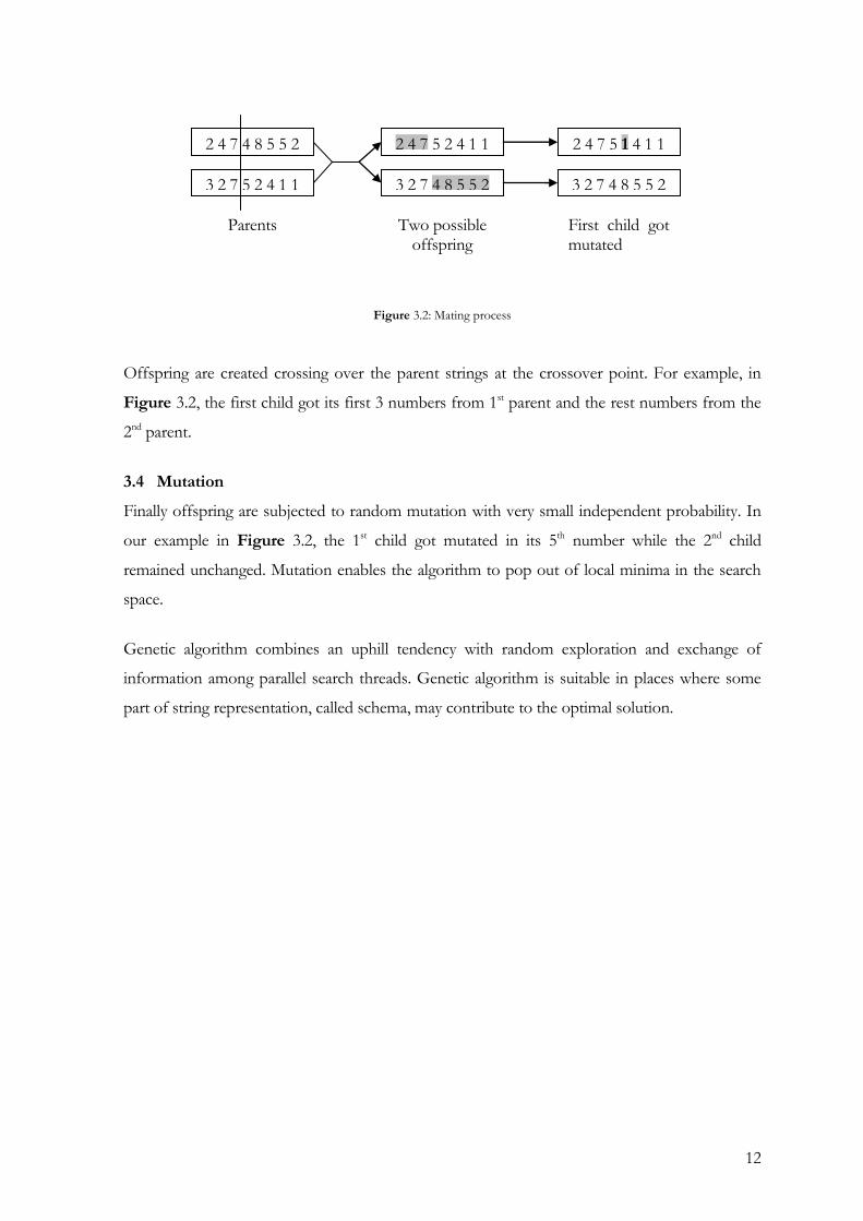
3.3 Cross-over

For each pair to be mated a crossover point is randomly chosen from the positions in the

string, e.g. in Figure 3.2 the crossover point is selected after the 3rd number.

12

Figure 3.2: Mating process

Offspring are created crossing over the parent strings at the crossover point. For example, in

Figure 3.2, the first child got its first 3 numbers from 1st parent and the rest numbers from the

2nd parent.

3.4 Mutation

Finally offspring are subjected to random mutation with very small independent probability. In

our example in Figure 3.2, the 1st child got mutated in its 5th number while the 2nd child

remained unchanged. Mutation enables the algorithm to pop out of local minima in the search

space.

Genetic algorithm combines an uphill tendency with random exploration and exchange of

information among parallel search threads. Genetic algorithm is suitable in places where some

part of string representation, called schema, may contribute to the optimal solution.

2 4 7 4 8 5 5 2

3 2 7 5 2 4 1 1

2 4 7 5 2 4 1 1

3 2 7 4 8 5 5 2

2 4 7 5 1 4 1 1

3 2 7 4 8 5 5 2

Parents Two possible offspring

First child got mutated

13

Figure 3.3: Genetic Algorithm

3.5 Conclusion

The problem being an NP-Hard problem, the optimality of the any solution cannot be claimed

to the best, and there is no deterministic algorithm to solve it. Genetic algorithm has been

chosen to solve the problem for its inherent feature of parallel search and the ability to get out

of local minima/maxima though the process of mutation. Genetic algorithm is also chosen

because in this problem because a good schema of the chromosome can actually lead to many

offspring of good fitness.

function GENETIC-ALGORITHM(population,FITNESS-FN) returns an

individual

inputs: population, a set of individuals

FITNESS-FN, a function that measures the fitness of an individual

repeat

new_population ← empty set

loop for i from 1 to SIZE( population ) do

x ← RANDOM-SELECTION( population,FITNESS-FN)

y ← RANDOM-SELECTION( population,FITNESS-FN)

child ← REPRODUCE(x,y)

if ( small random probability) then child ← MUTATE(child)

add child to new_population

population ← new_population

until some individual is fit enough , or enough time has elapsed

return the best individual in population, according to FITNESS-FN

function REPRODUCE(x,y) returns an individual

inputs: x,y, parent individuals

n ← LENGTH(x)

c ← random number from 1 to n

return APPEND( SUBSTRING(x,1,c),SUBSTRING(y,c+1,n))

14

Chapter 4 DEVELOPED

ALGORITHM

15

4.1 Developed Algorithm

The approach that has been taken to solve the given Strip-Packing problem was based on

Genetic Algorithm. The first issue was to represent the arbitrary shapes into some geometric

form.

4.2 Object definition

Each arbitrary shape was represented by an n-sided polygon. Each side of the polygon was a

straight line. Curves and other smoother shapes were approximated by sampling a curve at many

points and joining them with small lines. Therefore an arbitrary shape was represented by

A set of points P={P0,P1 … Pn}

A set of lines L={L0,L1 … Ln}

Where n+1 is the order of polygon. The polygon could be of both convex1 and non-convex1

type. Each line in the L, is directed and is described by a vector. Every polygon was oriented in

anti-clockwise direction as shown below:

Figure 4.1: A Polygon

1 A polygon is said to be convex if for every point inside the polygon a line is drawn in any direction it only intersects the polygon

itself at one single point. Otherwise the polygon is said to be non-convex.

P0

P1

P5

P4

P3

P2

L0

L1 L2

L3

L4 L5

16

4.3 Definitions

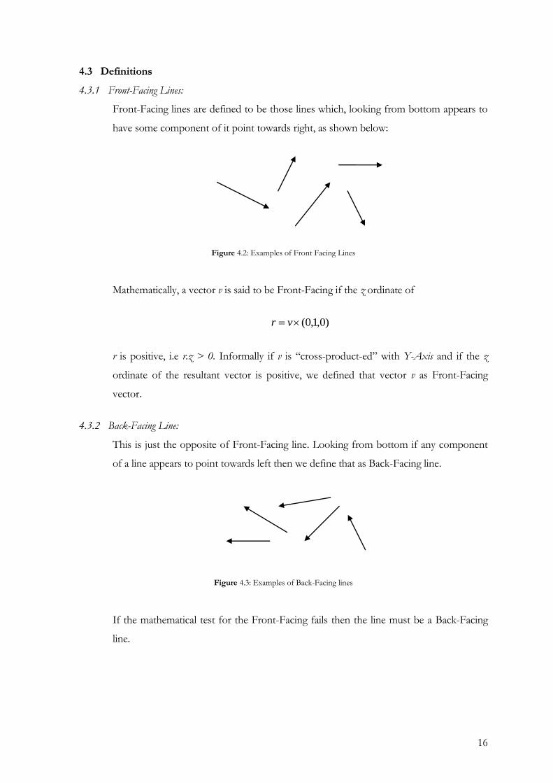
4.3.1 Front-Facing Lines:

Front-Facing lines are defined to be those lines which, looking from bottom appears to

have some component of it point towards right, as shown below:

Figure 4.2: Examples of Front Facing Lines

Mathematically, a vector v is said to be Front-Facing if the z ordinate of

)0,1,0( vr

r is positive, i.e r.z > 0. Informally if v is “cross-product-ed” with Y-Axis and if the z

ordinate of the resultant vector is positive, we defined that vector v as Front-Facing

vector.

4.3.2 Back-Facing Line:

This is just the opposite of Front-Facing line. Looking from bottom if any component

of a line appears to point towards left then we define that as Back-Facing line.

Figure 4.3: Examples of Back-Facing lines

If the mathematical test for the Front-Facing fails then the line must be a Back-Facing

line.

17

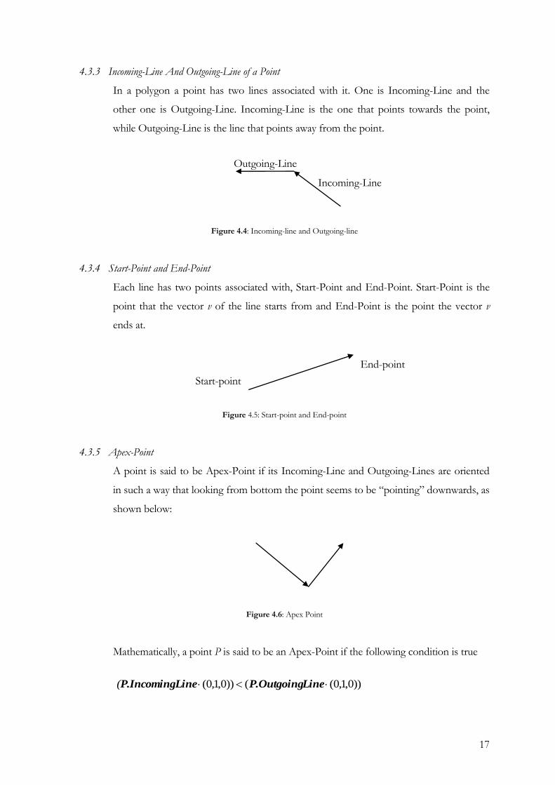
4.3.3 Incoming-Line And Outgoing-Line of a Point

In a polygon a point has two lines associated with it. One is Incoming-Line and the

other one is Outgoing-Line. Incoming-Line is the one that points towards the point,

while Outgoing-Line is the line that points away from the point.

Figure 4.4: Incoming-line and Outgoing-line

4.3.4 Start-Point and End-Point

Each line has two points associated with, Start-Point and End-Point. Start-Point is the

point that the vector v of the line starts from and End-Point is the point the vector v

ends at.

Figure 4.5: Start-point and End-point

4.3.5 Apex-Point

A point is said to be Apex-Point if its Incoming-Line and Outgoing-Lines are oriented

in such a way that looking from bottom the point seems to be “pointing” downwards, as

shown below:

Figure 4.6: Apex Point

Mathematically, a point P is said to be an Apex-Point if the following condition is true

))0,1,0(())0,1,0( LineP.OutgoingLineP.Incoming(

End-point

Start-point

Incoming-Line

Outgoing-Line

18

4.3.6 Crevice-Point

A point is said to be Crevice-Point if its Incoming-Line and Outgoing-Lines are oriented

in such a way that looking from bottom the point seems to be “pointing” upward, as

shown below:

Figure 4.7: Crevice-Point

Mathematically, if the condition of the Apex-Point fails, then the point must be a crevice

point.

4.3.7 Edge-Point

Edge point are those points whose either Incoming-Line or the Out-Going line is a

Back-Facing line while the other one is a Front-Facing line. For example:

Figure 4.8: Edge Points

4.4 Assumption

For our algorithm we ignored orientation, i.e. the orientation of the polygon will not be changed

and the same orientation will be used all through-out the algorithm and simulation process. This

types of requirement as usually posed in garments industry where cloth have a particular type of

“run” and all clothe pattern to be cut out must also align themselves in certain orientation to

match with that run. However, polygons can be translated (moved).

Edge Points

19

4.5 Mapping to GA

The first and the most important step in solving a problem using GA is to design/encode the

string representation (chromosome2). The given strip packing problem is such that there can be

no overlap between two polygons whatsoever. This restriction requires the chromosome to be

designed in such ways that even random generation of chromosomes guarantees that there will

not be any overlap between polygons.

4.5.1 Chromosome representation

Keeping that in mind, we designed our chromosome such that it has n number of genes (We

define chromosome as the string/array representation of a single state in GA. We also define

each basic element of that string/array as gene) where n is the number of total polygon to be fit

in the strip. Each gene has two information: “Sequence-Number” and “X-Position” and

associated with a particular polygon, which will be discussed shortly.

Figure 4.9: An example chromosome with 3 genes for 3 polygons.

4.5.2 Evaluating fitness value

The fitness of a particular chromosome is determined by traversing through all its genes

according to the Sequence-Number (which has a range of 0 to n-1) in ascending order, i.e. the

gene having the lowest Sequence-Number will be visited first and the highest Sequence-Number

will be visited last. For each gene visited, the corresponding polygon is allowed to drop freely

from a height which is the atleast equal to the worst possible height (hw) that could be generated

using all the polygon. This worst possible height can be found out once and very easily by

stacking all the polygon’s bounding box one over another and taking the total height (hw). With

y-ordinate set to hw, the polygon is dropped with x-ordinate set to X-Position information

stored in the gene. However, before dropping the polygon, the gene is checked if, with the given

X-Position, the polygon bound stays within the strip. In case the polygon bound doesn’t remain

within the strip, the X-Position information in the gene is modified so as to bring the polygon

bound within the strip. The process is illustrated in Figure 4.10.

Seq-No. X-Pos. Seq-No. X-Pos. Seq-No. X-Pos.

One Gene

20

As the polygon is dropped, collision detection tests are

Figure 4.10: Demonstrating the fitness evaluation process

performed to find if the polygon in question collides with polygons that had already been

dropped. If it collides, the collision points are calculated and the maximum distance the polygon

can move downward is also calculated and the polygon is allowed to fall that much distance

downward. This causes all the polygons to stack at the bottom of the strip according to the

information stored in all the genes and hence the chromosome. The maximum height required

(h) for all the polygons is noted and then the fitness value is calculated as follows

hhf w .............................................................................................................................. (4.1)

More the value of fitness f is, the lesser is the height (h) required to fit all the polygons and thus

represents a better solution.

4.5.3 Mating

Once the fitness value of all the chromosomes are found out, the population is allowed to mate

according to the standard GA algorithm, which was discussed earlier. However, instead of

a) The X-Position of the polygon is such that it made the polygon hang outside the strip bound.

b) The X-Position of the polygon is modified to bring the polygon bound inside the strip bound..

c) Finally the polygon is allowed to drop freely and collision detection tests are performed.

hw hw hw h

f

a b)

c)

X-Position

Modified X-Position

21

replacing the current generation with the new generation, we added the new generation of

chromosome to the old generation of chromosomes, thus increasing the population size. In the

process, we “killed” chromosome which had fitness value under a certain threshold. This

“killing” process kept the population size under some sort of check and allowed only the better

chromosomes to live through generations.

After running the above process for a certain number of generations, we would stop the

algorithm and output the best chromosome found so far.

4.6 Conclusion

Due to the inherent quality of GA to search for a solution in parallel fashion, combined with the

ability to pop out of local minima/maxima makes it a very suitable tool to generate a near

optimal solution. However, the biggest challenge of solving this particular problem with the

discussed scheme, the collision detection routine becomes the biggest bottleneck as far run-time

is concerned. Hence the collision detection routines need to be optimized.

22

Chapter 5 SIMULATION

FRAMEWORK

23

5.1 Simulation Framework

Our simulation framework is basically a stand-alone software that was built with a GUI support.

There are basically 3 modules, polygon input module, output module and GA-parameter input

module.

5.1.1 Our simulation framework consists of the following parameters

5.1.1.1 n number of arbitrary polygons.

Polygons are stored in simple text files which are read in by the simulation program.

5.1.1.2 Initial Population, k

Initially k number of chromosomes/individuals are created randomly. These k

chromosomes act as the first generation.

5.1.1.3 Number of Generations

This is basically the number of iterations or generations to be simulated for. Since the

problem is a NP-Hard problem, there is no particular sentinel condition so we need to

set this parameter manually.

5.1.1.4 Mutation probability such that 0 ≤ ≤ 1

This is the probability that determines if a new born chromosome is mutated in some

gene location. If mutation has to be performed, a gene location is selected in random

and then either of the “Sequence-Number” or the “X-Pos” would be mutated, i.e.

changed randomly. Changing “X-Pos” might render the polygon invalid because some

part of the polygon might hang outside the strip-bound. So after every mutation process,

the chromosome needs to be validated. Usually is set to very low probability and in

our simulation framework, we used a default value of 0.1.

5.1.1.5 Cull-Threshold such that 0 ≤ ≤ 1

This is the parameter that decides if a chromosome should be “killed” or kept alive

through generations. This is a normalized parameter and for every chromosome the

fitness value is also normalized between worst chromosome’s fitness value and the best

chromosome’s fitness value. For every chromosome, the normalized fitness NF is

calculated using the following formula:

fitnessosomeWorstChromfitnesssomeBestChromo

fitnessosomeWorstChromfitnessChromosomeNF

..

..

24

if NF < then the chromosome is “killed.”

5.2 Simulation software

The simulation software provides the user to input and change all the parameters that were

discussed in the previous section. The user can run the algorithm and watch how the average

fitness value of the population changes as well the plot of the best chromosome found so far.

The software also plots the population size. The user may also stop the simulation anytime

he/she feels like and see the output of the best result found so far.

Figure 5.1: Screenshot of the simulation software

The software takes polygon data as input in form of files which contains polygon vertices

information in textual format. It then provides the user to change several GA parameters like

initial population, mutation probability, number of generations etc.

The algorithm is run in a different thread so that the user interface can be interacted with while

the algorithm is running and user can cancel the operation at any time. The user can view the

best result produced so far graphically.

25

Since the software demanded graphical representation of the final result as well as ability to

graphically take input from user, a good GUI has been designed. For this GUI to be developed

a well renowned cross-platform GUI SDK has been used called wxWidget[10] which has built

in features for OpenGL.

The basic software operation can be summarized as follows.

Figure 5.2: Software Data Flow

Polygon Repository

GA Parameters

Genetic Algorithm

Main Software Module Graphical output of the results

Fitness Evaluator

Graph plotter for different information like Average

Fitness, Best-Fitness plot etc.

26

Chapter 6 OPTIMIZATION

27

6.1 Introduction

Since we relaxed ourselves from rotating the polygons, their orientation becomes static. As

polygons would be dropped from the top of the strip with fixed/static orientation we can pre-

calculate lots of collision data beforehand while loading the polygons.

6.2 Optimization

It can be noted that when a polygon is to be dropped from the top of the trip, only the

points/vertices of the front-facing lines can collide with the back-facing lines of the polygons

that had already been dropped. On the other hand, only the points/vertices of the back-facing

lines of the polygon already dropped in the strip can collide with the front facing lines of the

polygon to be dropped. This prunes out half of the vertices and lines to be tested for collision

on average and reduces the collision test to 1/4. The fact is demonstrated below.

Figure 6.1: Polygon Hit

In the above Figure 6.1, the bold lines of the top polygon are the front facing lines. The stripped

lines of the bottom polygon are the back-facing lines. All the points that belongs to the front-

facing lines of the top polygon are “collidable” points with the back-facing lines of the bottom

polygon. However, points marked with “stars” are crevice points with respect to the other

polygon. Crevice points can never contribute to collision, hence they are pruned. Points marked

with “box” are positioned in such way that they cannot contribute to any collision because the

polygon it belongs to has at least one line that blocks the point from colliding. Hence, these

points are also pruned. Lines that have both its point marked with “box” are pruned because

such line cannot contribute to a collision.

28

All the points marked with “circles” are front-collidable points of the top polygon which are

tested for collision with all the stripped lines (back-facing lines) of the bottom polygon. When

collision test is performed, an imaginary line is produced from the point to the given line and

tested if the following are true

If the imaginary line intersects with the other line

If the y-intercept of the intersection is lower or equal to the y-ordinate of the point.

If the point is found to collide with the line, the distance d between the point and the

intersection point is calculated. The same procedure is carried for all the back-facing points of

the bottom polygon with all the front-facing lines of the top. The minimum of all d is then used

to translate the top polygon downward.

All the back-facing lines, front-facing lines, front-collidable-points, back-collidable-points are

pre-calculated once the polygons are loaded and the results are simply used while finding the

fitness during GA. This roughly reduces the collision detection calculation for each pair of

polygon to almost ¼.

Two more optimization operations are also performed.

6.2.1 Potential Collidable Polygons

Before a polygon is dropped from the top, the lower end of the bounding box of the polygon is

extended till the bottom of the containing strip and then the resultant bounding box is tested for

overlap with all the bounding boxes of the polygons which had already been dropped. Only

those polygons that overlap with the extended bounding box may collide with the polygon

about to be dropped, and this set of polygons is termed as “Potential Collidable Polygons”

(PCP). This allows many polygons not to be tested for collision at all thus increasing

performance.

6.2.2 Height Pruning

Within the “PCP” if a collision is detected, and after translating the polygon, about to be

dropped, its y-ordinate of the lower corner of the bounding box is saved. When another

polygon of PCP has to be tested; if its y-ordinate of the top corner of the bounding box is less

than the y-ordinate already saved then the polygon is not tested at all. This prunes away all the

29

polygons that are far below in the stack of dropped polygon, thus increasing performance even

further.

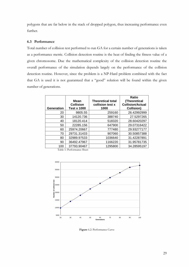
6.3 Performance

Total number of collision test performed to run GA for a certain number of generations is taken

as a performance metric. Collision detection routine is the heat of finding the fitness value of a

given chromosome. Due the mathematical complexity of the collision detection routine the

overall performance of the simulation depends largely on the performance of the collision

detection routine. However, since the problem is a NP-Hard problem combined with the fact

that GA is used it is not guaranteed that a “good” solution will be found within the given

number of generations.

Generation

Mean Collision

Test x 1000

Theoretical total collision test x

1000

Ratio (Theoretical

Collision/Actual Collision)

20 9805.55 259160 26.42992999

30 14120.736 388740 27.5297265

40 18120.414 518320 28.60420297

50 22285.156 647900 29.07316422

60 25974.20667 777480 29.93277177

70 29731.31433 907060 30.50857388

80 32989.97533 1036640 31.42287891

90 36492.47967 1166220 31.95781735

100 37793.90467 1295800 34.28595197 Table 1: Performance Sheet

5000

10000

15000

20000

25000

30000

35000

40000

20 30 40 50 60 70 80 90 100

Generations

Nu

mb

er

of

co

llis

ion

te

st

Figure 6.2: Performance Curve

30

The relationship between no. of generation and total number of collision test is fairly linear.

The “Theoretical” number of collision test is the number of collision test we would need to

perform if there weren’t any optimization. Table 1 tells that the optimization that we applied to

solve the problem reduced the execution time by almost 30 times. Moreover this improvement

over “Theoretical” number seems to be getting better as the number of generation is increasing.

6.4 Conclusion

Optimization in the collision detection algorithm is very important as it happens to the major

bottleneck of the whole system. Table 1 clearly shows the almost 30 times less operations are

performed due the optimization performed.

31

Chapter 7 RESULTS

32

7.1 Introduction

The current system has several input parameters, they are as follows:

Initial Population Size

Number of Generations

Mutation Probability

Set of Polygons

In this section we will study the effect of various parameters on the output of the algorithm.

While studying one parameter we will keep other parameters constant and observe the output.

For all the experiment conducted below, 7 polygons were used with a total vertex count of 191.

Following are the polygons that were used in the experiment.

Figure 7.1: Polygons used in experiment

33

7.2 Effect of mutation-probability

This experiment was conducted to test the effect of mutation probability on the final output.

Number of generations was set to 100, while initial population size was set to 1000 for this

experiment.

400

420

440

460

480

500

520

0.1 0.2 0.3 0.4 0.5 0.6 0.7 0.8 0.9 1

Mutation Probabilty

Avera

ge F

itn

ess o

f th

e p

op

ula

tio

n

Figure 7.2: Mutation probability Vs Average fitness

692

693

694

695

696

697

698

699

700

701

702

0 0.2 0.4 0.6 0.8 1 1.2

Mutation Probability

Av

era

ge B

est

Fit

nes

s

Figure 7.3: Mutation Probability Vs Average Best Fitness

34

The mutation probability was changed and the corresponding average fitness of the population

was observed.

7.2.1 Interpretation

Mutation was introduced in Genetic Algorithm to let GA pop out of local minima and maxima.

However, this mutation probability needs to be set to very small value. As mutation probability

increases, more individual get mutated and the algorithm converges to “blind” random search.

As the algorithm becomes more “blindly” random, the average fitness value decreases.

However, setting the mutation probability to too low will make the algorithm unable to pop out

of local minima or maxima. This also makes the average fitness of the population go low. In the

experiment it can be seen that mutation probability of around ~0.2 produces the best result.

Although Figure 7.3 shows that mutation probability of around ~0.5 gives the best result but

this might have happened due to shortage of data in our test cases. Usually the better picture is

grasped in the average fitness curve.

7.3 Effect of Number of Generation

This experiment was conducted with the mutation probability set to 0.2 and the initial

population set to 1000. The number of generations was increased and each time the average

fitness of the population as well as the best fitness was observed.

350

400

450

500

550

600

10 30 50 70 90 110 130 150

No. of generations

Av

era

ge

fit

of

po

pu

lati

on

Figure 7.4: No. of Generations Vs Average fit of population

35

655

660

665

670

675

680

685

690

695

700

0 20 40 60 80 100 120 140 160

No. of Generation

Av

g B

es

t F

it C

hro

mo

so

me

Figure 7.5: No. of generation Vs Average Best Fit

7.3.1 Interpretation

It can be noted that as the number of generation is increased the average fitness of the

population increases. This is explained by the fact that mutation probability is set to 0.2 (low)

and since good individual has the greater probability to mate, the average fitness of the

population approaches the best fitness.

However, increasing the number of generations doesn’t monotonically increase the fitness of the

best individual found so far. This can be explained by the fact that once a good individual is

found, it becomes extremely hard to beat that individual any by the grace of GA we happened to

find the good solutions by 100 generations.

36

7.4 Effect of Initial Population Size

This experiment was conducted to test the effect of initial population size on the final result. For

this experiment, the mutation probability was set to 0.2, and number of generation was set to

100.

670

675

680

685

690

695

700

705

0 200 400 600 800 1000 1200 1400 1600

Initial Population Size

Avera

ge B

est

Fit

ness

Figure 7.6: Initial population size Vs Average Best Fitness

37

495

500

505

510

515

520

525

530

535

540

0 200 400 600 800 1000 1200 1400 1600

No. of initial population

Av

era

ge

Fit

ne

ss

of

Po

pu

lati

on

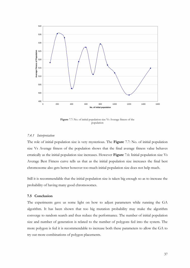
Figure 7.7: No. of initial population size Vs Average fitness of the population

7.4.1 Interpretation

The role of initial population size is very mysterious. The Figure 7.7: No. of initial population

size Vs Average fitness of the population shows that the final average fitness value behaves

erratically as the initial population size increases. However Figure 7.6: Initial population size Vs

Average Best Fitness curve tells us that as the initial population size increases the final best

chromosome also gets better however too much initial population size does not help much.

Still it is recommendable that the initial population size is taken big enough so as to increase the

probability of having many good chromosomes.

7.5 Conclusion

The experiments gave us some light on how to adjust parameters while running the GA

algorithm. It has been shown that too big mutation probability may make the algorithm

converge to random search and thus reduce the performance. The number of initial population

size and number of generation is related to the number of polygons fed into the system. The

more polygon is fed it is recommendable to increase both these parameters to allow the GA to

try out more combinations of polygon placements.

38

Chapter 8 CONCLUSION

39

8.1 Conclusion

This thesis proposed a very simple algorithm to solve the specific problem of garments industry.

In the garments industry clothes shapes are needed to be cut out of long running strip of cloth

but the orientation of the shapes need not to be changed. This is because every cloth has a

particular “run” and when cloth shapes are cut its orientation has to conform to that run.

There are many algorithms which solves the problem of packing arbitrary shapes. However, the

orientation posed a big problem and introduced both run-time and computational complexity

which we could easily avoid in our thesis.

We first surveyed all the available related algorithms; there are only a few of them. Then we first

defined and formulated the problem at hand. The nature of the problem made us chose Genetic

Algorithm as the major tool to solve the problem. We presented our new approach with detailed

description of Genetic Algorithms. We then presented several result outputs and interpretation

of each output generated. While interpreting we tried to show how the results are dependant on

each of the input parameters of problem. We also showed all the possible areas where we

optimized the algorithm.

We hope we have been able to propose a new and good approach, based wholly on Genetic

Algorithm, to find out a near-optimal solution for packing a set of arbitrary polygon with fixed

orientation in a strip with an aim to minimize the total height required.

We also showed how various GA parameters and other parameters can be find tuned to

generate much better results.

40

References

[1] Stuart Russel, Steven Norvig, “Genetic Algorithm”, Artificial Intelligence-A Modern Approach, 2nd Edition, pp. 116-119. [2] Stuart Russel, Steven Norvig, “Neural Networks”, Artificial Intelligence-A Modern Approach, 2nd Edition, pp. 736-748. [3] Liu Hu Yao, He Yuan Jun, “Algorithm for 2D irregular-shaped nesting problem based on the NFP

algorithm and lowest-gravity-center principle,” Journal of Zhejiang University SCIENCE A. 2006 Vol. 7 No.4 p. 570-576.

[4] Armando Ponce-Pérez, Arturo Pérez-Garcia and Victor Ayala-Ramirez,” Bin-Packing Using

Genetic Algorithms” 15th International Conference on Electronics, Communications and Computers (CONIELECOMP'05) pp. 311-314.

[5] E.Hopper and B.C.H.Turton. A review of the application of meta-heuristic algorithms to 2D strip packing problems. Artificial Intelligence Review, 16 (2001), 257-300.

[6] Kathryn A.Dowsland and William B.Dowsland. Solution approaches to irregular nesting problems. European Journal of Operational Research, 84(1995), 506-521.

[7] Art RC. An approach to the two dimensional irregular cutting stock problem. IBM Cambridge Scientific Centre, Report 36-Y08, 1966. [8] Adamowicz M, Albano A. Nesting two dimensional shapes in rectangular modules. Computer Aided Design, 8, 1 (1976), 27-33. [9] Julian Smart and Kevin Hock, “Cross-Platform GUI Programming with wxWidgets.”