SINGULARITIES AND MIXING INFLUID MECHANICS

By

Xiaoqian Xu

A dissertation submitted in partial fulfillment of the

requirements for the degree of

Doctor of Philosophy

(Mathematics)

at the

UNIVERSITY OF WISCONSIN – MADISON

2016

Date of final oral examination: April 27, 2016

The dissertation is approved by the following members of the Final Oral Committee:

Alexander Kiselev, Professor, Mathematics

Andrej Zlatos, Professor, Mathematics

Serguei Denissov, Professor, Mathematics

Jean-Luc Thiffeault, Professor, Mathematics

Saverio E. Spagnolie, Assistant Professor, Mathematics

i

Abstract

Among the most important and most difficult open problems in the field of analysis are

questions about the behavior of solutions to differential equations modeling the dynamics

of fluids. The main issues that one must overcome in addressing them are frequently

the nonlinearity and nonlocality of these equations. In this thesis we study these and

related models, focusing on the possibility of singularity formation for their solutions as

well as on ways such singular behavior can be suppressed.

In the first chapter of this thesis, we discuss the small scale creation and possible

singularity formation in PDEs of fluid mechanics, especially the Euler equations and the

related models. Recently, Tom Hou and Guo Luo proposed a new scenario, so called the

hyperbolic flow scenario, for the development of a finite time singularity in solutions to

3D incompressible Euler equation. We first give a clear and understandable picture of

hyperbolic flow restricted in 1D. Then, based on the recent work by Alexander Kiselev

and Vladimir Sverak, we look into the hyperbolic geometry in 2D. Finally, we go back

to 3D problem, and analyze a simplified 1D model for the potential singularity of the

3D Euler equation by Tom Hou and Guo Luo.

In the second chapter of this thesis, we investigate the problem about how to suppress

the blowup. At the end of the second chapter, we demonstrate that incompressible

mixing flow can indeed arrest the finite time blow up phenomenon. We first concentrate

on understanding the mechanisms involved in mixing, studying mixing properties of the

flows with different structure, and finding most efficient mixing flows. We resolve the

problem of finding the optimal lower bound of the “mixing norm” under an enstrophy

ii

constraint on the velocity field. On the basis of this result, we evaluate the role of mixing

in systems where chemotaxis is present. We prove the result that the presence of fluid

flow can affect singularity formation by mixing the density thus making concentration

harder to achieve. This is an example to show that the fluid advection can regularize

singular nonlinear dynamics.

This thesis resulted in the publications [31,32,48,57,87].

iii

To my parents and my beloved wife

iv

Acknowledgments

Foremost, I would like to express my deepest gratitude to my advisor, Professor Alexan-

der Kiselev for the consistent support and advice, and especially for his patient when

talking math to me. I could not have imagined having a better advisor for my PhD

study. I would also like to thank him for being as a caring friend, and always ready to

talk to me and help me out.

I would like to thank my co-advisor, Professor Andrej Zlatos, who really helps me a

lot. I see him as a role model, for both his great achievements in math, his hard working

and his rigorous attitude. I would also like to thank him for his kind help when I was

in difficult situation.

I want to thank the rest of my committee, Professor Serguei Denissov, Professor

Jean-Luc Thiffeault and Professor Saverio E. Spagnolie. Thanks them for attending

my defense, reading this thesis and provide insightful comments. Also thanks them for

introducing me to many different areas of math.

I would like to thank Professor Andreas Seeger, for introducing me the harmonic

analysis and for his helping about finishing the paperwork.

I thank all my awesome friends, Dr. Yao Yao, Dr. Kyudong Choi, Dr. Vu Hoang,

Dr. Marie Radosz, Dr. Changhui Tan, Dr. Lei Li, Dr. Zhennan Zhou, Dr. Qin Li, Dr.

Lu Wang, Professor Shi Jin, Professor Gautam Iyer, Mr. Tam Do, Mr. Pengfei Liu and

Dr. Yu Sun, for their helpful discussions, support and friendship. I would like to thank

Tam Do separately, for his expertising in both math and food, and for his good advice. I

would also like to thank the staff members in UW Madison math department, especially

v

Kathie Keyes and Christopher Uhlir, for their help to make the paperwork much easier.

Last but not least, I would like to thank my family. Thanks to my father and mother,

Jianzhong Xu and Xinying Li, for their unconditional love and support all these years.

Thanks to my wife, Tianyan, for all her support, understanding and unwavering love to

me. I am so lucky to have you!

vi

Contents

1 Singularity Formation for Some Active Scalar Equations 1

1.1 Introduction . . . . . . . . . . . . . . . . . . . . . . . . . . . . . . . . . . 1

1.1.1 1D model . . . . . . . . . . . . . . . . . . . . . . . . . . . . . . . 2

1.1.2 2D Euler equation . . . . . . . . . . . . . . . . . . . . . . . . . . 4

1.1.3 A modified 1D model . . . . . . . . . . . . . . . . . . . . . . . . . 5

1.2 Hyperbolic fluid flow: 1D model equations . . . . . . . . . . . . . . . . . 7

1.2.1 Model discussion and the main results . . . . . . . . . . . . . . . 8

1.2.2 Euler 1D model . . . . . . . . . . . . . . . . . . . . . . . . . . . . 10

1.2.3 α-patch 1D model . . . . . . . . . . . . . . . . . . . . . . . . . . . 19

1.3 Hyperbolic fluid flow: fast growth in 2D Euler equation . . . . . . . . . . 22

1.3.1 Main result . . . . . . . . . . . . . . . . . . . . . . . . . . . . . . 23

1.3.2 The key lemma . . . . . . . . . . . . . . . . . . . . . . . . . . . . 24

1.3.3 The proof of the main theorem . . . . . . . . . . . . . . . . . . . 37

1.4 Stability of blow-up for a 1D model of 3D Euler equation . . . . . . . . . 41

1.4.1 Derivation of model equations and the main results . . . . . . . . 42

1.5 Periodic Case . . . . . . . . . . . . . . . . . . . . . . . . . . . . . . . . . 43

1.6 Perturbation . . . . . . . . . . . . . . . . . . . . . . . . . . . . . . . . . . 58

2 Mixing by Fluid Flow 64

2.1 Introduction . . . . . . . . . . . . . . . . . . . . . . . . . . . . . . . . . . 64

2.1.1 Mixing . . . . . . . . . . . . . . . . . . . . . . . . . . . . . . . . . 64

vii

2.1.2 Preventing blow-up by mixing . . . . . . . . . . . . . . . . . . . . 67

2.2 Lower bounds on the mix norm of scalars advected by enstrophy-constrained

flows . . . . . . . . . . . . . . . . . . . . . . . . . . . . . . . . . . . . . . 70

2.2.1 Main result and discussion . . . . . . . . . . . . . . . . . . . . . . 70

2.2.2 Rearrangement Costs and the Proof of the Main Theorem. . . . . 73

2.2.3 Proofs of Lemmas. . . . . . . . . . . . . . . . . . . . . . . . . . . 76

2.3 Preventing blow-up by mixing . . . . . . . . . . . . . . . . . . . . . . . . 81

2.3.1 Main result and the interpretation . . . . . . . . . . . . . . . . . . 82

2.3.2 Finite time blow up . . . . . . . . . . . . . . . . . . . . . . . . . . 84

2.3.3 Global existence: the L2 criterion . . . . . . . . . . . . . . . . . . 93

2.3.4 An H1 condition for an absorbing set in L2 . . . . . . . . . . . . . 96

2.3.5 The approximation lemma . . . . . . . . . . . . . . . . . . . . . . 99

2.3.6 Proof of the main theorem: the relaxation enhancing flows . . . . 101

2.3.7 Yao-Zlatos flow . . . . . . . . . . . . . . . . . . . . . . . . . . . . 110

2.3.8 Discussion and generalization . . . . . . . . . . . . . . . . . . . . 118

A Direct calculation of lemma 1.5.2 121

B Real line case of the stability result 144

C Some inequalities in Keller-Segel equation 149

Bibliography 154

1

Chapter 1

Singularity Formation for Some

Active Scalar Equations

1.1 Introduction

The following transport equation

ωt + u · ∇ω = 0. (1.1)

is a basic mathematical model in fluid dynamics. If u depends on ω, (1.1) is called an

active scalar equation. The problem of deciding whether blowup can occur for smooth

initial data becomes very hard if the dependence of ω is nonlocal in space.

The relationship expressing u in terms of ω is commonly called Biot-Savart law. We

have the following examples in 2D:

u = ∇⊥(−4)−1ω, (1.2)

where ∇⊥ = (−∂y, ∂x) is the perpendicular gradient. Equations (1.1) and (1.2) are the

vorticity form of 2D Euler equation. When we take

u = ∇⊥(−∆)−12ω,

(1.1) becomes the surface quasi-geostrophic (SQG) equation, which has important ap-

plications in geophysics, or can be regarded as a toy model for the 3D Euler equations.

2

For more details we refer to [19].

The 3D incompressible Euler equation describes the motion of an ideal (inviscid

and incompressible) fluid. Whether the solution of this equation exists globally has

remained open for over 250 years and has a close connection to the Clay Millennium

Prize Problem on the Navier-Stokes equations [1]. Recently, Tom Hou and Guo Luo

proposed a new scenario for the development of a finite time singularity in solutions

to 3D axisymmetric Euler equation at a boundary point in [44]. This part of this

thesis involves development of the analytical approach to understand this new numerical

simulation based on analyzing some active scalar equations.

1.1.1 1D model

In [44], so called hyperbolic flow scenario was proposed to obtain singular solutions for

the 3D Euler equations. The hyperbolic flow scenario in two dimensions can be explained

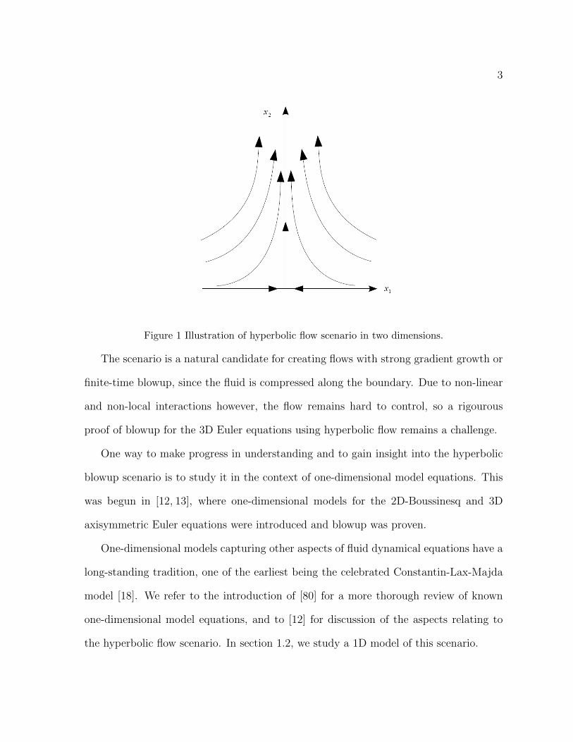
in the following way. Consider e.g. a flow in the upper half-plane x2 > 0. The essential

properties required are (see Figure 1 for an illustration):

• There is a stagnant point of the flow at one boundary point (e.g. the origin) for

all times.

• Along the boundary, the flow is essentially directed towards that point for all times.

Such flows can be created by imposing symmetry and other conditions on the initial

data. For incompressible flows the stagnant point is a hyperbolic point of the velocity

field, hence the name.

3

Figure 1 Illustration of hyperbolic flow scenario in two dimensions.

The scenario is a natural candidate for creating flows with strong gradient growth or

finite-time blowup, since the fluid is compressed along the boundary. Due to non-linear

and non-local interactions however, the flow remains hard to control, so a rigourous

proof of blowup for the 3D Euler equations using hyperbolic flow remains a challenge.

One way to make progress in understanding and to gain insight into the hyperbolic

blowup scenario is to study it in the context of one-dimensional model equations. This

was begun in [12, 13], where one-dimensional models for the 2D-Boussinesq and 3D

axisymmetric Euler equations were introduced and blowup was proven.

One-dimensional models capturing other aspects of fluid dynamical equations have a

long-standing tradition, one of the earliest being the celebrated Constantin-Lax-Majda

model [18]. We refer to the introduction of [80] for a more thorough review of known

one-dimensional model equations, and to [12] for discussion of the aspects relating to

the hyperbolic flow scenario. In section 1.2, we study a 1D model of this scenario.

4

1.1.2 2D Euler equation

The 1D models may help people to understand the hyperbolic scenario intuitively, nev-

ertheless we still need to look into the incompressibility structure, which can hardly be

modelled by 1D model. In section 1.3, we study the 2D Euler equation given by (1.1)

and (1.2).

Global regularity of solutions to 2D Euler equation is well-known, it was first proved

in [86] and [39], and see also [50], [68], [11] for more work. By the standard estimates

(see [89]), to obtain the higher regularity of the solution corresponding to smooth initial

data, we only need to bound the L∞ norm of the gradient of vorticity. The best known

upper bound for this quantity has double exponential growth in time. This result is

well-known and has first appeared in [89].

The sharpness of the double exponential growth bound has remained open for a long

time. In [90], Yudovich provided an example showing unbounded growth of the vorticity

gradient at the boundary of the domain. Nadirashvili [73] constructed an example on the

annulus where the gradient of vorticity grows linearly in time. In recent years, Denisov

did a series of work on this problem. In [26], he constructed an example on the torus

with superlinear growth in time. In [27], he proved that double exponential growth can

be possible for any fixed but finite time. In [28], he constructed a patch solution to

smoothly forced 2D Euler equation where the distance of two patches decreases double

exponentially in time. We refer to [56] and [92] for more information on these questions.

In 2014, Kiselev and Sverak [56] constructed an example of initial data in the disk

where such double exponential growth was observed. This means the double exponential

growth in time is the best upper bound we can get for the gradient of vorticity, at least for

5

solutions to 2D Euler equation in the disk. How generic is such growth is an interesting

question. If this growth happens in many situations, it would highlight the challenges

involved into numerical simulation of the solutions. In section 1.3, we make the first

step towards better understanding of this question, by generalizing the construction

of Kiselev and Sverak to the case of an arbitrary sufficiently regular domain with a

symmetry axis. The main new ingredient of our proof is a more general version of the

key lemma in [56]. The lemma captures hyperbolic structure of the velocity field near

the point on the boundary where the fast growth happens. The analysis in [56] is specific

to the disk, and the Green’s function estimates used to prove the lemma do not translate

easily to the more general case. We develop a more flexible natural construction that

allows to carry the estimates through.

1.1.3 A modified 1D model

The main purpose of section 1.4 is to generalize the results of [12]. In [12], the authors

derive a 1D model to study regularity for axisymmetric 3D Euler with swirl, which is

the following system:

∂t

(ωθ

r

)+ ur

(ωθ

r

)r

+ uz(ωθ

r

)z

= −(

(ruθ)2

r4

)z

, (1.3)

∂t(ruθ) + ur(ruθ)r + uz(ruθ)z = 0, (1.4)

where ur and uz can be calculate by the following equations:

ur =ψzr, (1.5)

uz = −ψrr, (1.6)

6

where ψ satisfies the following elliptic equation:

1

r

∂

∂r

(1

r

∂ψ

∂r

)+

1

r2

∂2ψ

∂z2= ω. (1.7)

One can write ur and uz in terms of ω by computing the Green’s function of the above

elliptic PDE, more details can be found on [67].

The 1D model was inspired by the numerics presented in [44], which strongly suggest

singularity formation on the boundary of a cylindrical domain. The 1D model suggested

by Hou and Luo [44] to study the dynamics near the boundary is following:

ωt + uωx = θx (1.8)

θt + uθx = 0 (1.9)

ux = Hω (1.10)

where H is the Hilbert transform and the space domain is taken to be R or S1(periodic).

Equivalently, we can write u as

u(x, t) = k ∗ ω(x, t) where k(x) =1

πlog |x|. (1.11)

In [12], blow up is shown for (1.8)-(1.10) for a large class of smooth initial data.

There are numerous related 1D models that have been used to study fluid equations.

One of the earliest of these models was the one proposed by Constantin-Lax-Majda [18],

which have later inspired other models [25] [21]. We refer the reader to [12] for a survey

of results on this subject.

In section 1.4, for one of our results, we generalize their results to the model with

the following choice of Biot-Savart law:

u(x, t) = k ∗ ω(x, t) where k(x) =1

πlog

|x|√x2 + a2

. (1.12)

7

Using the reduction scheme from [12] to reduce 3D Euler to a 1D system, we will see that

(1.12) is perhaps a more natural choice of Biot Savart law in section 1.4.1. The choice

of (1.11) considerably simplifies estimates needed to prove finite time blow-up. In the

section ??, we prove blow up of the system (1.8) and (1.9) with law (1.12). The main

task will be to prove estimates that allow the framework for the blow-up with (1.11) to

remain.

For our second and closely related result, we prove the solutions to (1.8), (1.9) with

even more generalized kernels can blow-up as well. We will modify (1.11) by adding a

smooth function, which preserve the symmetries of (1.8), (1.9). The details will be in

section ??. To prove blow-up, in vague terms, we show that to “leading order” that the

dynamics which lead to (1.8)-(1.10) to form singularity persist even with a more general

law. Below, it will be apparent that our first result is not a direct corollary of our second

result as we will see that the class of initial data used in the first result will be larger.

One can think of our results as strengthening the case for studying this family of

equations. By proving singularity formation for more general Biot-Savart laws, one can

view the blow up of (1.8)-(1.10) as not being solely the result of algebraic cancellations

and manipulations due to the particular choice of Biot-Savart law, but as a more general

phenomenon.

1.2 Hyperbolic fluid flow: 1D model equations

The results in this section come from a joint work with Tam Do, Vu Hoang and Maria

Radosz [31].

8

1.2.1 Model discussion and the main results

In this section, we will study 1D models of (1.1) on R with the following two choices of

u:

ux = Hω, (1.13)

u = (−∆)−α2 ω = −cα

∫R|y − x|−(1−α)ω(y, t) dy. (1.14)

The choice (1.13) leads to a 1D analogue of the 2D Euler equation. One arrives at this

model simply by restricting the dynamics to the boundary. In section 1.2.2 we give

a brief heuristic argument which works by assuming that ω is concentrated in a small

boundary layer.

We note that the model (1.13) was mentioned in [12], where it was stated that (1.13)

has properties analogous to the 2D Euler equation, without giving details. In particular,

in [12] a 1D model of the 2D Boussinesq equations (an extended version of (1.13)) was

introduced and studied. One of our goals here is to validate the 1D model introduced

in [12] in a setting where comparison with 2D results are available. The fact shown

below, that the solutions to the model problem (1.13) behave similarly to the full 2D

Euler case, provides support to the usefulness of the extended version of this model

in [12] for getting insight into behavior of solutions to 2D Boussinesq system and 3D

Euler equation.

The model defined by (1.14) is called α-patch model and appears in [35] (also with

viscosity term). From the regularity standpoint, the α-patch model is between 1D Euler

(ux = Hω) and the Cordoba-Cordoba-Fontelos model (u = Hω) (see [21, 80]), which is

an analogue of the SQG equation. These two models differ however from a geometric

perspective, since the symmetry properties of the Biot-Savart laws are different. For the

9

CCF model, the velocity field is odd for even ω, whereas (1.14) is odd for odd ω. It is

important to choose data with the right symmetry to make u odd, and thus to create a

stagnant point of the flow at the origin for all times.

We note that local existence and blowup results for (1.14) were given in [35], where

also dissipation is allowed. There the authors rely on a suitable Lyapunov function to

show blowup, whereas we emphasize the more geometric aspects in this section. That

is, we will be studying the analogue of the hyperbolic flow scenario for the above 1D

models and show that this leads to natural and intuitive constructions of solutions with

strong gradient growth and finite-time blowup.

Another blowup result related to hyperbolic flow was recently proven by A. Kiselev,

L. Ryzhik, Y. Yao and A. Zlatos [55] and concerns a α-patch model in 2D for small

α > 0.

In this section, we will prove the following theorems.

Theorem 1.2.1. The solution ω to (1.1) and (1.13) satisfies the following inequality:

‖ωx‖L∞ 6 C(1 + ‖(ω0)x‖) exp(eCt),

for some universal C, provided that the initial data ω0 is smooth. And there is ω0 such

that the equality holds.

Theorem 1.2.2. There exists smooth initial data ω0, such that the solution to (1.1) and

(1.14) blows up in finite time.

10

1.2.2 Euler 1D model

1.2.2.1 Heuristic derivation.

Recall the 2D Euler equations in vorticity form

ωt + u · ∇ω = 0

where u = ∇⊥(−∆)−1ω.

We first indicate a simple heuristic motivation for the choice (1.13) (see also [12]).

Consider the 2D Euler equation in a half-space x2 > 0 and denote x = (x1,−x2). The

x1-component of the velocity (up to a normalization constant) for compactly supported

vorticity ω is given by

u1(x, t) = −∫R2

(y2 − x2)

|y − x|2ω(y, t) dy (1.15)

where ω has been extended to x2 6 0 by odd reflection (ω(x, t) = −ω(x, t)).

Suppose now that ω is concentrated in a boundary layer of width a > 0 and that

ω(x1, x2, t) = ω(x1, t) in this boundary layer. Then a calculation gives

u1(x1, 0, t) = −2

∫R

log

((y1 − x1)2 + a2

(y1 − x1)2

)ω(y1, t) dy1. (1.16)

If we now retain only the singular part of the kernel log(z2+a2

z2

)∼ −2 log |z| and identify

u with u1, we get (dropping the constants)

u(x, t) =

∫R

log |y − x|ω(y, t) dy.

So a reasonable 1D model is

ωt + uωx = 0, ux = Hω, ω(x, 0) = ω0(x) (x, t) ∈ R× [0,∞). (1.17)

11

where H is the Hilbert transform, using the convention

Hω(x, t) = P.V.

∫ω(y, t)

x− ydy.

For this model, we have the following local well-posedness property:

Proposition 1.2.3. Given initial data ω0 ∈ Hm0 ((0, 1)) with m > 2, there exists T =

T (‖ω0‖Hm0

) > 0 such that the system has a unique classical solution ω ∈ C([0, T ];Hm0 ).

The proof is standard so we skip it here.

An alternative argument to motivate (1.13) is to observe that the gradient of the 2D

Euler velocity is given by a zero-th order operator acting on ω. In one dimension, this

leaves only the choice ux = cHω or ux = cω, c being a nonzero constant. So we could

also consider the model

ωt + uωx = 0, ux = −ω, ω(x, 0) = ω0(x) (x, t) ∈ R× [0,∞). (1.18)

(1.18) is however not a close analogue of 2D Euler (see remark 1.2.7).

1.2.2.2 Sharp a-priori bounds for gradient growth.

We will first prove the global regularity of the solution to equation (1.17) by showing

that ωx can grow at most with double exponential rate in time. Then we will give

an example of a smooth solution to (1.17) where such growth of the gradient of ω is

achieved, meaning the bound is sharp.

Due to the Biot-Savart law relating u and ω, the proof of an upper bound for

‖ωx(·, t)‖∞ is very similar to the proof for the full 2D Euler equations. For the reader’s

convenience, we give the proof. Recall first the definition of the Holder norm

||ω||Cα = sup|x−y|61,x 6=y

|ω(x)− ω(y)||x− y|α

12

for compactly supported ω.

We will need an estimate on the Hilbert transform:

Lemma 1.2.4. Let 0 < α < 1. Suppose supp(ω) ⊂ [−D(t), D(t)] and assume without

loss of generality that ||ω0||L∞ = 1. Then

‖ux‖∞ 6 C(α) (1 + | log(D(t))|+ log(1 + ‖ω‖Cα))

Proof. For any δ > 0, we have∣∣∣∣∫[−D(t),D(t)]\(x−δ,x+δ)

ω(y)

x− ydy

∣∣∣∣ 6 C

∫ D(t)

δ

1

ydy 6 C(| log δ|+ | log(D(t))|).

Using the oddness of 1x, we have∣∣∣∣P.V.∫ x+δ

x−δ

ω(y)

x− ydy

∣∣∣∣ =

∣∣∣∣∫ x+δ

x−δ

1

x− y(ω(y)− ω(x)) dy

∣∣∣∣ 6 C(α)‖ω(x, t)‖Cαδα.

Choosing δ = min

1, ( 1‖ω‖Cα

)1α

, we get the desired estimate of ‖ux‖∞.

The following lemma gives an estimate on D(t).

Lemma 1.2.5. Suppose the support of ω0 is in [−1, 1] and ||ω0||L∞ = 1. Then the sup-

port of ω(x, t) will be inside [−C exp(CeCt), C exp(CeCt)], for some universal constant

C > 0.

Proof. Suppose suppω = [−D(t), D(t)]. Then for any point x inside of this interval, we

have

|u(x)| 6∫ D(t)

−D(t)

| log |x− y|| dy 6 C

∫ 2D(t)

0

| log |s|| ds 6 CD(t)(| log(D(t))|+ 1).

By following the trajectory of the particle at D(t),

D′(t) 6 CD(t)(| log(D(t))|+ 1).

13

A simple argument using differential inequalities shows that D(t) is always less than

z(t), where z(t) is the solution of

z′(t) = Cz(t)(log z(t) + 1), z(0) = minD(0), 2.

This yields the double-exponential upper bound on D(t).

The following Theorem gives the double exponential upper bound for ωx.

Theorem 1.2.6. There is universal constant C such that if ω0 is smooth, compactly

supported with suppω0 ⊂ [−1, 1] and ‖ω‖L∞ = 1,

log(1 + ‖ωx‖L∞) 6 C log(1 + ‖(ω0)x‖L∞)eCt (t > 0). (1.19)

Proof. We follow the proof in [56]. Let us denote the flow map corresponding to the

evolution by Φt(x). Then

∂

∂tΦt(x) = u(Φt(x), t), Φ0(x) = x,

and ∣∣∣∣∂t|Φt(x)− Φt(y)||Φt(x)− Φt(y)|

∣∣∣∣ 6 ||ux||L∞ .After integration, and by Lemma 1.2.4 and Lemma 1.2.5, this gives

f(t)−1 6|Φt(x)− Φt(y)||x− y|

6 f(t),

where

f(t) = exp

(C

∫ t

0

(1 + exp(Cs) + log(1 + ||ωx||L∞)) ds

).

This bound also holds for Φ−1t . On the other hand,

‖ωx‖L∞ = supx 6=y

|ω0(Φ−1t (x))− ω0(Φ−1

t (y))||x− y|

6 ‖(ω0)x‖ supx 6=y

|Φ−1t (x)− Φ−1

t (y)||x− y|

.

14

Which means we have

(1 + ‖ωx‖L∞) 6 (1 + ‖(ω0)x‖L∞) exp

(C

∫ t

0

1 + exp(Cs) + log(1 + ‖ωx‖L∞) ds

),

or

log(1 + ‖ωx‖L∞) 6 log(1 + ‖(ω0)x‖L∞) + C exp(Ct) + C

∫ t

0

(1 + log(1 + ‖ωx‖L∞)) ds.

So y(t) := log(1 + ‖ωx‖L∞) satisfies the integral inequality

y(t) 6 y(0) + CeCt +

∫ t

0

(1 + y(s)) ds

and by the integral form Gronwall’s inequality and some elementary manipulations, we

arrive at the bound y(t) 6 C1y(0)eC2t. This yields the desired bound on ‖ωx‖∞.

Remark 1.2.7. If we choose our Biot-Savart law to be ux = −ω, then from a modifica-

tion of the above proof we get an exponential upper bound for ‖ωx‖L∞. This is different

from the 2D Euler equation, which suggests that (1.17) is a better analogue of the 2D

Euler equation than (1.18). Moreover the equation (1.18) also has different symmetry

properties.

Next we construct initial data ω0 such that ‖ωx(·, t)‖L∞ grows with double-exponential

rate, proving the sharpness of the a-priori bound (1.19). The hyperbolic flow scenario

is created in the following way: First, we require that the initial data ω0 is odd with

respect to the origin, and has compact support. By Proposition 1.2.3, the oddness is

easily seen to be preserved by the evolution. Consequently, the velocity field (which is

also an odd function) can be written as

u(x, t) = −x∫ ∞

0

K

(x

y

)ω(y, t)

ydy (x > 0), (1.20)

15

where

K(s) :=1

slog

∣∣∣∣s+ 1

s− 1

∣∣∣∣ . (1.21)

Note that the origin is a stagnant point of the flow for all times. By taking ω0 to be

positive on the right, the direction of the flow is towards the origin. More precisely, ω0

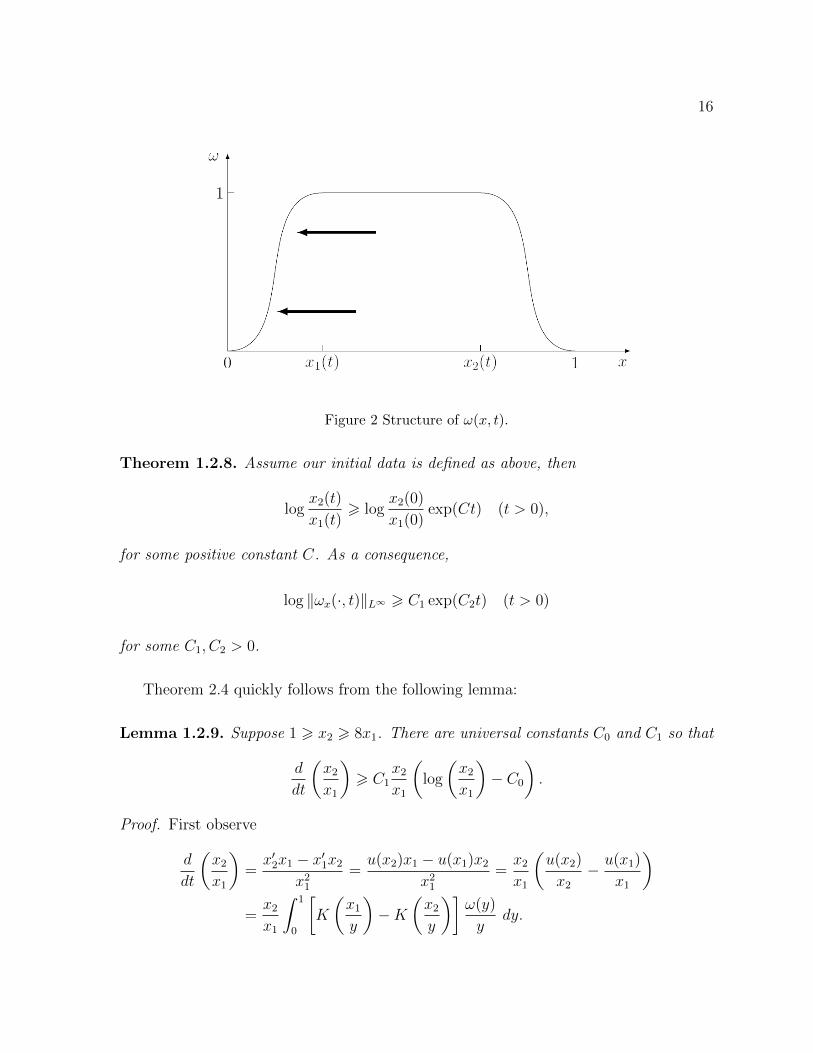
is defined as follows (see Figure 2):

• Let ω0 be supported on [−1, 1], smooth and odd. Choose numbers 0 < x1(0) <

2x2(0) < 1 such that Mx1(0) 6 x2(0) where M will be determined later. Require

that ω0 is increasing on [0, x1(0)], decreasing on [x2(0), 1] and identically 1 on

[x1(0), x2(0)].

Using the earlier notation Φt for the flow map associated to (1.17), let

x1(t) := Φt(x1(0))

x2(t) := Φt(x2(0))

It is easy to see that the general structure of ω0 will be preserved by the flow: For fixed

t, ω(x, t) will be increasing on [0, x1(t)], decreasing on [x2(t), 1] and identically 1 on

[x1(t), x2(t)]. In fact, since u(x, t) 6 0 for x > 0, x1(t) and x2(t) will be moving towards

the origin in time. We will show that the quantity x2(t)x1(t)

increases double exponentially

in time. This is sufficient to conclude the desired growth of ‖ωx(·, t)‖L∞ .

16

Figure 2 Structure of ω(x, t).

Theorem 1.2.8. Assume our initial data is defined as above, then

logx2(t)

x1(t)> log

x2(0)

x1(0)exp(Ct) (t > 0),

for some positive constant C. As a consequence,

log ‖ωx(·, t)‖L∞ > C1 exp(C2t) (t > 0)

for some C1, C2 > 0.

Theorem 2.4 quickly follows from the following lemma:

Lemma 1.2.9. Suppose 1 > x2 > 8x1. There are universal constants C0 and C1 so that

d

dt

(x2

x1

)> C1

x2

x1

(log

(x2

x1

)− C0

).

Proof. First observe

d

dt

(x2

x1

)=x′2x1 − x′1x2

x21

=u(x2)x1 − u(x1)x2

x21

=x2

x1

(u(x2)

x2

− u(x1)

x1

)=x2

x1

∫ 1

0

[K

(x1

y

)−K

(x2

y

)]ω(y)

ydy.

17

We decompose the integral into 4 pieces which we will estimate separately:∫ 1

0

[K

(x1

y

)−K

(x2

y

)]ω(y)

ydy

=

∫ 2x1

0

+

∫ 12x2

2x1

+

∫ 2x2

12x2

+

∫ 1

2x2

[K

(x1

y

)−K

(x2

y

)]ω(y)

ydy

=I + II + III + IV.

For I, we use 0 6 ω(y) 6 1 and 2x1 6 x2 6 1:

0 6 I 6∫ 2x1

0

1

x1

log(x1 + y)

|x1 − y|dy +

∫ 2x1

0

1

x2

log(x2 + y)

|x2 − y|dy

=1

x1

3x1 log 3 +1

x2

[2x1 log

1 + 2x1x2

1− 2x1x2

+ x2 log

(1− 2x1

x2

)+ x2 log

(1 +

2x1

x2

)]

6 3 log 3 + 2 log 2.

Using the fact that K(s) is increasing in [0, 1) and decreasing in (1,∞] and that ω(y) = 1

for y ∈ (2x1,12x2) we get

II =

∫ 12x2

2x1

[K

(x1

y

)−K

(x2

y

)]ω(y)

ydy >

∫ 12x2

2x1

(2− 1

2log(3))

1

ydy

= (2− 1

2log(3)) log

(x2

x1

)− C.

Using the positivity of K,

III =

∫ 2x2

12x2

[K

(x1

y

)−K

(x2

y

)]ω(y)

ydy > −

∫ 2x2

12x2

K

(x2

y

)ω(y)

1

ydy

> −∫ 2

12

1

s2log|s+ 1||s− 1|

ds > −C.

We estimate IV in the following way, using that ω(y) 6 1 and x1y

6 x2y

6 1 for 2x2 6

18

y 6 1:

|IV | =∣∣∣∣∫ 1

2x2

[K

(x1

y

)−K

(x2

y

)]ω(y)

ydy

∣∣∣∣ 6 ∫ 1

2x2

[K

(x2

y

)−K

(x1

y

)]1

ydy

6∫ 1

2x2

1

x2

logy + x2

y − x2

dy −∫ 1

2x2

1

x1

logy + x1

y − x1

= (i)− (ii).

We can compute (i) directly and get

(i) =1

x2

log1 + x2

1− x2

+ log(1 + x2)(1− x2)− 2 log(x2)− 3 log(3).

Similarly, for (ii), we have

(ii) =1

x1

log1 + x1

1− x1

+ log(x1 + 1)(1− x1)− 2x2

x1

log2x2 + x1

2x2 − x1

− log(2x2 + x1)(2x2 − x1).

Then using that x1 < x2,

|IV | 6 C − 2 log(x2) + log(4x22 − x2

1) = C − log

(4−

(x1

x2

)2)

6 C.

The proof of Theorem 1.2.8 is now completed as follows: choose M > 8 so large such

that 12

log(M)−C0 > 0. We have thus 12

log(x02x01

)−C0 > 0. From Lemma 1.2.9 it follows

that x2(t)x1(t)

is growing in time and that we have

d

dt

(x2

x1

)>C1

2

x2

x1

log

(x2

x1

),

or ddt

log(x2x1

)> C1

2log(x2x1

)for all times. This clearly implies that x2

x1grows double-

exponentially.

19

Remark 1.2.10. In [56], the Biot-Savart law is decomposed into a main contribution

and an error term. In our case (1.20), the main contribution would be

−x∫ ∞x

ω(y)

ydy. (1.22)

If we replace (1.20) by (1.22), then double-exponential growth of x2x1

can be proven by

a straightforward argument. In this case, the computation for the estimate in Lemma

1.2.9 becomes much easier.

1.2.3 α-patch 1D model

In this section, we consider the 1D model equation

ωt + uωx = 0 (1.23)

with a different Biot-Savart law

u(x, t) = (−∆)−α/2ω(x, t) = −cα∫R|y − x|−(1−α)ω(y, t) dy, α ∈ (0, 1) (1.24)

For convenience, we will assume the constant cα associated with the fractional Laplacian

is 1, and we write γ = 1− α.

This problem has been studied in [35], where local existence and uniqueness results

for smooth initial data are proven. From these, we can show that this equation preserves

oddness and u(0, t) = 0 holds with odd initial datum. For odd data, we can write

u(x, t) = −∫ ∞

0

k(x, y)ω(y, t) dy (1.25)

where k(x, y) = |y − x|−γ − |y + x|−γ. Note that k(x, y) > 0 for x 6= y ∈ (0,∞).

Following similar ideas as for 1D Euler, we specifiy our initial data ω0 as follows:

20

• Pick 0 < x1(0), x2(0) with Mx1(0) < x2(0). Let ω0 be smooth, odd, ω0(x) > 0 for

x > 0 and have its support in [−2x2(0), 2x2(0)]. M > 1 is to be chosen below. Let

ω0 moreover be bounded by 1, smoothly increasing in the interval [0, x1(0)] and

ω0 = 1 between x1(0) and x2(0).

As long as the solution remains smooth, the general structure of the solution does not

change. Let x1(t), x2(t) be again the position of the particles starting at x1(0), x2(0).

Theorem 1.2.11. There exists a choice of x1(0), x2(0),M and a time T > 0 such that

the smooth solution of (1.23) for the above initial data cannot be continued beyond T .

Provided the solution remains smooth on the time interval [0, T ), the particle starting at

x1(0) reaches the origin at time t = T , i.e.

limt→T

x1(t) = 0. (1.26)

In this sense, the solution forms a “shock”.

Remark 1.2.12. In [35], the existence of blowup solutions to (1.23) is shown using

energy methods. The advantage is that they are able to include a dissipation term.

The drawback of energy methods in general, however, is that the blowup mechanism is

obscured. Our proof uses the dynamics of the solution and gives a more intuitive picture

of the blowup, and is easily generalized to other even kernels having the same singular

behavior.

In the rest of this section, we will prove Theorem 1.2.11. First of all, we track the

movement of the particle starting at x1(0), which is the following lemma.

Lemma 1.2.13. There exists a universal constant M > 2 so that if Mx1(t) 6 x2(t),

21

the velocity at x1(t) will satisfy

u(x1(t), t) 6 −Cx1(t)1−γ, (1.27)

for some universal constant C.

Proof. Let u1 = u(x1(t), t). Since k, ω > 0 on (0,∞)

−u1 >∫ x2

2x1

k(x1, y) dy

= cγ[−(x2 + x1)1−γ + (x2 − x1)1−γ + (3x1)1−γ − x1−γ

1

]= cγ

[(31−γ − 1)x1−γ

1 + (x2 − x1)1−γ − (x2 + x1)1−γ]= cγx

1−γ1

[(31−γ − 1) +

1

x1−γ1

((x2 − x1)1−γ − (x2 + x1)1−γ)]

for some constant cγ > 0. Note that (31−γ − 1) > 0. We can write

1

x1−γ1

(x2 − x1)1−γ − (x2 + x1)1−γ =x1−γ

2

x1−γ1

[(1− x1

x2

)1−γ

−(

1 +x1

x2

)1−γ]

=:x1−γ

2

x1−γ1

f(x1/x2).

There exists a constant C > 0 with |f(x1/x2)| 6 C|x1/x2| for |x1/x2| 6 1/2, and so

−u1 > cγx1−γ1

[(31−γ − 1)− CM−γ]

if Mx1(t) 6 x2(t). Now choose M large enough so that CM−γ is smaller than the

number 12(31−γ − 1).

This estimate of velocity field will lead to a blowup in finite time, provided we can

show Mx1(t) 6 x2(t). More precisely,

d

dtx1(t) = u(x1) 6 −Cx1−γ

1 ,

22

implying

x1 6 C(x1(0)γ − Ct)1γ .

This shows that no later than T0 := C−1x1(0)γ, the particle x1(t) will reach the origin,

and the solution cannot be continued smoothly. Note that T0 does not depend on x2(0).

It remains therefore to control the motion of x2(t), concluding the proof.

Lemma 1.2.14. For x2(0) large enough, Mx1(t) < x2(t) for t ∈ [0, T0).

Proof. We write u(x2(t), t) = u2. Observe that the support of ω(·, t) is always contained

in [−2x2(0), 2x2(0)] because of u(x, t) 6 0 for x > 0.

Next we find an upper bound on u2:

|u2(t)| 6∫ 2x2(0)

−2x2(0)

|y − x|−γ 6 Cx2(0)1−γ. (1.28)

Hence,

x2(t) > x2(0)−∫ T0

0

|u2(s)| ds > x2(0)(1− Cx2(0)−γT0). (1.29)

Now choose x2(0) so large that Mx1(0) < x2(0)(1− Cx2(0)−γT0). But then

Mx1(t) 6Mx1(0) < x2(0)(1− Cx2(0)−γT0) 6 x2(t),

giving the statement of the Lemma.

1.3 Hyperbolic fluid flow: fast growth in 2D Euler

equation

The results in this section come from [87].

23

1.3.1 Main result

Recall the two dimensional Euler equation in vorticity form for an incompressible fluid

is given by

∂tω + (u · ∇)ω = 0, ω(x, 0) = ω0(x). (1.30)

Here ω = curl u is the vorticity of the flow, and the velocity u can be determined from

ω by the Biot-Savart law. Here we consider the flow in a smooth bounded domain Ω,

and we assume u satisfies a no flow boundary condition, namely u · n = 0 on ∂Ω, here

n is the outer normal vector of ∂Ω. This implies that

u = ∇⊥∫

Ω

GΩ(x, y)ω(y)dy.

WhereGΩ(x, y) is the Green’s function of the Dirichlet problem in Ω and∇⊥ = (∂x2 ,−∂x1)

is the perpendicular gradient.

In this section, we will prove the following double exponential growth bound for more

general domains instead of disk:

Theorem 1.3.1. Let Ω be a C3 bounded open domain in R2, tangent at the origin to

the x1-axis and symmetric about x2-axis. Consider the 2D Euler equation on Ω. There

exists a smooth initial data ω0 with ‖∇ω0‖L∞ > ‖ω0‖L∞ such that the corresponding

solution ω(x, t) satisfies

‖∇ω(·, t)‖L∞‖ω0‖L∞

>

(‖∇ω0‖L∞‖ω0‖L∞

)c(Ω) exp(c(Ω)‖ω0‖L∞ t)

(1.31)

for some c(Ω) > 0 that only depends on Ω and for all t > 0.

Based on the ideas of [56], we will focus on the appropriate representation for the

Biot-Savart law for the fluid velocity u. The key will be obtaining the representation

24

which will show that u1 ∼ x1 log(x1) on appropriate (time dependent) length scales.

After that, based on the construction of [56], we will get the desired growth for the

gradient of vorticity in domain Ω.

1.3.2 The key lemma

To construct a flow with fast growth in the gradient, we need a technical lemma for the

expansion of velocity field.

We use the same notation as in [56], which means ω is the vorticity field in Ω, odd in the

first variable. Note that this property is conserved by Euler evolution in a symmetric

domain. Let u be the corresponding velocity field. D+ = x ∈ Ω : x1 > 0, x = (−x1, x2)

and Q(x1, x2) is a region that is the intersection of D+ and the quadrant y : x1 6 y1 <

∞, x2 6 y2 <∞.

Lemma 1.3.2. [Key Lemma.] Suppose Ω is a C3 bounded open domain in R2, symmetric

about x2-axis, and tangent to x1-axis at the origin. Take any γ, π2> γ > 0. Denote

Dγ1 the intersection of D+ with a sector π

2− γ > φ > −π

2, where φ is the usual angular

variable. Then there exists δ > 0 such that for all x ∈ Dγ1 such that |x| 6 δ we have

u1(x, t) = − 4

πx1

∫Q(x1,x2)

y1y2

|y|4ω(y, t)dy + x1B1(x, t), (1.32)

where |B1(x, t)| 6 C(γ,Ω)‖ω0‖L∞.

Similarly, if we denote Dγ2 the intersection of D+ with a sector π

2> φ > γ, then for all

x ∈ Dγ2 such that |x| 6 δ, we have

u2(x, t) =4

πx2

∫Q(x1,x2)

y1y2

|y|4ω(y, t)dy + x2B2(x, t). (1.33)

where |B2(x, t)| 6 C(γ,Ω)‖ω0‖L∞.

25

In the argument below, δ and constant C may change from line to line, but since we

change it only for finite many times, at the end we choose the smallest δ and the biggest

C among all of them instead.

We want to define y∗ to be the mirror image point of y, about the boundary. Namely,

we want y∗ to be written as y∗ = 2e(y)− y, where e(y) is a point on ∂Ω so that y− e(y)

is orthogonal to the tangent line at e(y). More intuitively, e(y) is the closest point to

y on ∂Ω. However, it is not clear that this e(y) is well-defined. Given y, it may be

possible to find more than one e(y) on the whole ∂Ω. However, we will show y∗(y) is

locally well-defined close to the origin by lemma 1.3.3 below.

Since ∂Ω is tangent to the x1 axis at the origin, we can choose the parameterization

near the origin of ∂Ω such that we have ∂Ω = (s, f(s)) for some function f ∈ C3 and

sufficiently small s.

Lemma 1.3.3. There exists r = r(Ω) > 0 only depending on Ω, so that for any y ∈

Br(0) ∩ Ω, there is a unique s in (−2r, 2r) such that the following equation holds:

(s− y1) + f ′(s)(f(s)− y2) = 0. (1.34)

Moreover, this s, as a function of y, is C2.

Remark 1.3.4. If we call e(y) = (s(y), f(s(y))), then (1.34) means y−e(y) is orthogonal

to the tangent line of ∂Ω at e(y). Note that if e(y) is one of the points on ∂Ω closest to

y then (1.34) holds.

Proof of lemma 1.3.3. We call the left hand side of (1.34) the function F (s, y). We take

derivative of F (s, y) in s and get

1 + f ′(s)2 + f ′′(s)(f(s)− y2). (1.35)

26

So DsF (0, (0, 0)) = 1 and F (0, (0, 0)) = 0. Thus by implicit function theorem we know

the solution to (1.34) exists and is unique in a neighborhood of 0 × (0, 0). By

choosing r small enough, s(y) is uniquely defined. Moreover, as in the very beginning

we choose ∂Ω to be C3, which means f is C3. Hence, F (s, y) is a C2 function as it

only contains function f ′ and f , which means s(y) is C2 in y by the implicit function

theorem.

By lemma 1.3.3, we can give the following definition:

Definition 1.3.5. Given r small enough, for any |y| 6 r, we define e(y) to be the only

point in B2r(0) ∩ ∂Ω so that e(y) − y is orthogonal to the tangent line of ∂Ω at e(y).

And we define y∗(y) = 2e(y)− y. We denote y∗(y) = (y∗1(y), y∗2(y)) = (y∗1, y∗2).

Then, we have the following lemma.

Lemma 1.3.6. Take r small enough as in lemma 1.3.3. If |s0| 6 2r and y ∈ Br(0)∩Ω,

we have

y∗1 − s0 =1− f ′(s0)2

1 + f ′(s0)2(y1 − s0) +

2f ′(s0)

1 + f ′(s0)2(y2 − f(s0)) +O(|y − (s0, f(s0))|2),

y∗2 − f(s0) =2f ′(s0)

1 + f ′(s0)2(y1 − s0) +

f ′(s0)2 − 1

1 + f ′(s0)2(y2 − f(s0)) +O(|y − (s0, f(s0))|2).

(1.36)

Here the constant in capital O notation only depends on the domain Ω. In addition the

map y∗ is invertible in y in Br(0) ∩ Ω.

Proof of lemma 1.3.6. This is an elementary calculation by Taylor’s expansion formula.

Like in the proof of lemma 1.3.3, we call the left hand side of (1.34) F (s, y). We take

the partial derivative of F (s, y) with s = s(y) in y1 and denote ∂1 = ∂y1 , ∂2 = ∂y2 . We

27

get

∂1s− 1 + f ′(s)2∂1s+ f ′′(s)∂1s(f(s)− y2) = 0.

Plug in y1 = s0 ,y2 = f(s0), noticing that we have s(s0, f(s0)) = s0, we get

∂1s|y=(s0,f(s0)) =1

1 + f ′(s0)2.

Which means by the definition of y∗ we get

∂1y∗1|y=(s0,f(s0)) = 2∂1s|y=(s0,f(s0)) − 1 =

1− f ′(s0)2

1 + f ′(s0)2

And similarly by taking the partial derivative in y2 in F (s, y) we get

∂2s|y=(s0,f(s0)) =f ′(s0)

1 + f ′(s0)2.

So

∂2y∗1|y=(s0,f(s0)) = 2∂2s|y=(s0,f(s0)) =

2f ′(s0)

1 + f ′(s0)2

By chain rule, we get

∂1f(s)|y=(s0,f(s0)) =f ′(s0)

1 + f ′(s0)2, ∂2f(s)|y=(s0,f(s0)) =

f ′(s0)2

1 + f ′(s0)2.

Which means we can get

∂1y∗2|y=(s0,f(s0)) =

2f ′(s0)

1 + f ′(s0)2, ∂2y

∗2|y=(s0,f(s0)) =

f ′(s0)2 − 1

1 + f ′(s0)2.

Thus by Taylor’s expansion we get (1.36). And we can also see the invertibility of y∗ for r

small enough, this is simply by the inverse function theorem because | det(∇y∗)|y∈∂Ω| =

1.

To understand y∗ better, we need another lemma. The following lemma shows that

although ∂Ω could be crazy, the intuition that y∗ must be outside of Ω is always true.

28

Lemma 1.3.7. There exists r so that for any y ∈ Br(0) ∩ Ω, y∗(y) /∈ Ω.

Proof of lemma 1.3.7. First, since y is close to the origin, the slope of inner normal line

at e(y) of ∂Ω is close to +∞. Recall by our definition the inner normal line has the

same direction as y − e(y), which means the second component of e(y) is less than y2.

By the definition of y∗, y∗2 < y2.

Now we argue by contradiction. Suppose for every r0 we can find y so that y∗(y) is inside

Ω. By the expansion of y∗ near zero, we know that |y∗| ≈ |y|. Here the notation ” ≈ ”

means there are constants C1, C2 only depending on Ω, such that C1|y| 6 |y∗| 6 C2|y|.

So, if r0 is small enough, say, less than rC2

, where r is the same r in lemma 1.3.3, then

y∗(y) is also in the domain of map y∗ by lemma 1.3.3. By definition, e(y) − y∗(y) is

orthogonal to the tangent line at e(y). However, by lemma 1.3.3, such a boundary point

e(y) is unique, which means e(y) = e(y∗(y)). So we know y∗(y∗(y)) = y. But then

y2 = y∗(y∗(y))2 < y∗2 < y2, which is a contradiction.

We will use y∗ as a sort of conjugate point for y in the context of the Dirichlet

reflection principle for the representation of the Green’s function. We note that for the

case of the disk in [56], by the well known explicit formula for the Green’s function, the

natural choice of y∗ is given by circular inversion of y. For more general Ω the choice of

y∗ is less obvious. We will see that our definition of y∗ will work well for the estimates

that we have in mind.

Without loss of generality, we assume Ω ⊂ [−2, 2] × [−2, 2]. Then we have the

following proposition.

Proposition 1.3.8. Suppose Ω is a C3 bounded open domain in R2, symmetric about

x2-axis, and tangent to x1-axis at the origin. Then there exists r = r(Ω) > 0 so that for

29

x, y ∈ Br(0), the Green function of Ω can be written as:

GΩ(x, y) =1

2π(log |x− y| − log |x− y∗|) +B(x, y). (1.37)

Here B(x, y) satisfies for any ω ∈ L∞(Ω),∫Br(0)∩Ω

B(x, y)ω(y)dy ∈ C2,α(Br(0)∩Ω), for

any 0 < α < 1. More precisely, we have

‖∂xi∂xj∫Br(0)∩Ω

B(x, y)ω(y)dy‖L∞(Br(0)∩Ω) 6 C(Ω)‖ω‖L∞ i, j = 1, 2

To prove this proposition, we need a technical lemma.

Lemma 1.3.9. Let x = (s, f(s)). Let K(z1, z2) be a integral kernel such that it is

C1 on the set z1 ∈ Ω, z2 ∈ Ω : z1 6= z2. Suppose we have K(s, f(s), y) = O( 1|x−y|)

and DsK(s, f(s), y) = O( 1|x−y|2 ). Then

∫ΩK(s, f(s), y)ω(y)dy has modulus of continuity

s log(s), with the constant equal to C(Ω)||ω||L∞. Here C(Ω) is a constant that only

depends on Ω.

Proof of lemma 1.3.9. Without loss of generality, let s1 < s2. Suppose |s1−s2| = ζ. Let

( (s1+s2)2

, f( (s1+s2)2

)) be Z. By the smoothness of f , there is a constant C1 = C1(Ω), so

that for any s between s1 and s2, (s, f(s)) ∈ BC1ζ(Z). Then, for any τ > C1ζ, we have∫Ω

(K(s1, f(s1), y)−K(s2, f(s2), y))ωdy

=

∫Ω∩Bτ (Z)

(K(s1, f(s1), y)−K(s2, f(s2), y))ω(y)dy+∫Ω∩Bcτ (Z)

(K(s1, f(s1), y)−K(s2, f(s2), y))ω(y)dy

6 C||ω||L∞∫

Ω∩Bτ (Z)

(1

|y − (s1, f(s1))|+

1

|y − (s2, f(s2))|)dy+

C||ω||L∞∫

Ω∩Bcτ (Z)

∫ s2

s1

|DsK(t, f(t), y)|dtdy

(1.38)

30

For y ∈ Bτ (Z), by the smoothness of f ,

|y − (si, f(si))| 6 |y − Z|+ |Z − (si, f(si))| 6 τ + C1ζ,

for i = 1, 2. In addition, for any s1 6 s 6 s2 and y ∈ Bcτ (Z), we have

|y − (s, f(s))| > |y − Z| − |Z − (s, f(s))| > τ − C1ζ.

Hence, the right hand side of (1.38) is no more than

C||ω||L∞∫

(Ω−Z)∩Bτ+C1ζ(O)

1

|y|dy + C||ω||L∞

∫(Ω−Z)∩Bcτ−C1ζ

(O)

|s1 − s2||y|2

dy 6

C||ω||L∞(

∫ τ+C1ζ

0

1

r· rdr +

∫ 2

τ−C1ζ

ζ

r2· rdr)

= C||ω||L∞(τ + ζ log(τ − C1ζ) + C1ζ).

(1.39)

Here Ω − Z means the translation of Ω by Z. So if we choose τ = 4C1ζ, we get the

desired modulus of continuity.

Remark 1.3.10. In this lemma, it’s easy to see that if K(s, f(s), y) is not differentiable

but |K(s1, f(s1), y)−K(s2, f(s2), y)| = |s1−s2|αO( 1|(s1,f(s1))−y|2 + 1

|(s2,f(s2)−y)|2 ), we can still

get the similar result. More precisely,∫

ΩK(s, f(s), y)ω(y)dy has modulus of continuity

xα log(x). This can be used to extend the results of this section to less regular domains

with C2,α boundary.

Now we prove proposition 1.3.8.

Proof of proposition 1.3.8. The idea is to use the properties of elliptic equations.

First, remember

B(x, y) = GΩ(x, y)− 1

2π(log |x− y| − log |x− y∗|),

31

where GΩ(x, y) is the Green function of domain Ω, y∗ is a function of y defined by

definition 1.3.5. As a well-known result, Green function is a smooth function for x 6= y.

Here we would like to show the subtraction of 12π

log |x− y|, which is the Green function

of R2, can eliminate the singularity of GΩ(x, y) with the help of the term log |x− y∗|.

As a result of lemma 1.3.7, we know that for all y, y∗ /∈ Ω. Therefore for any fixed

y ∈ Ω, log |x − y∗| is smooth and harmonic in x. This means B(x, y) is harmonic as x

varies in Ω, and satisfies the boundary condition B(x, y)|x∈∂Ω = 12π

log( |x−y∗|

|x−y| ). Hence∫Ω∩Br(0)

B(x, y)ω(y)dy is also harmonic and satisfies∫Ω∩Br(0)

B(x, y)ω(y)dy|x∈∂Ω∩Br(0) =

∫Ω∩Br(0)

1

2πlog(|x− y∗||x− y|

)ω(y)dy.

Since the boundary of the domain Ω is C3, by the well-known results on elliptic regularity

(see, e.g., Lemma 6.18 of [37]), we know that in order to show that∫

Ω∩Br(0)B(x, y)ω(y)dy

is C2,α near the origin, we only need to show that this harmonic function is C2,α on the

boundary near the origin. Recall the notation x = (s, f(s)). We only need

ι(s) =

∫Ω∩Br(0)

1

2πlog(|(s, f(s))− y∗||(s, f(s))− y|

)ω(y)dy (1.40)

to be C2,α in s for s small. Here remember y∗ is only a function in y, so ι(s) is a well

defined function in s. The proof for regularity of ι is simply by calculation. Here we

will only use the expansion of x − y∗ and the corresponding cancellation of y − y∗. As

ι(s) can be seen as the integral of a difference of the same function in different points

y and y∗, we will essentially need to calculate the finite differences of some complicated

functions.

First we find the second derivative in s of log( |(s,f(s))−y∗||(s,f(s))−y| ). We call it K(s, f(s), y).

32

More precisely, we have

−K(s, µ, y) =1 + f ′′(s)(µ− y2) + f ′(s)2

|x− y|2− 2

((s− y1) + f ′(s)(µ− y2))2

|x− y|4

− 1 + f ′′(s)(µ− y∗2) + f ′(s)2

|x− y∗|2+ 2

((s− y∗1) + f ′(s)(µ− y∗2))2

|x− y∗|4.

(1.41)

Then, observe that by lemma 1.3.6 and simple computation, for y close to (s, f(s)) we

have f(s)−y∗2 = f(s)−y2+O(|f(s)−x2|)+O(|s−x1|)+O(|x−y|2) = f(s)−y2+O(|x−y|),

which means y2− y∗2 = O(|x− y|) for y close to x, and |x− y∗|2 = |x− y|2 +O(|x− y|3),

for x, y close to the origin and y close to x. So K(s, f(s), y) can be written as

f ′′(s)(f(s)− y2 +O(|x− y|)) +O(|x− y|))|x− y|2 +O(|x− y|3)

−

2A(s, y)(s− y1 + s− y∗1 + f ′(s)(f(s)− y2 + f(s)− y∗2))

|x− y|4 +O(|x− y|5)+

2((s− y1) + f ′(s)(f(s)− y2))2O(|x− y|)

|x− y|4 +O(|x− y|5).

(1.42)

Where A(s, y) = (s− y1)− (s− y∗1) + f ′(s)((f(s)− y2)− (f(s)− y∗2))). By lemma 1.3.6,

A(s, y) = (s− y1) +1− f ′(s)2

1 + f ′(s)2(y1 − s) +

2f ′(s)

1 + f ′(s)2(y2 − f(s))+

f ′(s)

(f(s)− y2 +

2f ′(s)

1 + f ′(s)2(y1 − s) +

f ′(s)2 − 1

1 + f ′(s)2(y2 − f(s))

)+

O(|x− y|2)

=−2f ′(s)2

1 + f ′(s)2(y1 − s) +

2f ′(s)

1 + f ′(s)2(y2 − f(s))+

f ′(s)

(2f ′(s)

1 + f ′(s)2(y1 − s) +

−2

1 + f ′(s)2(y2 − f(s))

)+O(|x− y|2)

= O(|x− y|2).

(1.43)

Again by lemma 1.3.6 we have s− y∗1 = O(|x− y|), f(s)− y∗2 = O(|x− y|). And also we

have s− y1 = O(|x− y|) and f(s)− y2 = O(|x− y|). Plug in all of these into (1.42) we

get K(s, f(s), y) = O( 1|x−y|).

33

Then, we take the derivative of K(s, f(s), y) in terms of s again. We get

DsK(s, f(s), y) =f ′′′(s)(f(s)− y2) + 3f ′′(s)f ′(s)

|x− y|2−

(1 + f ′′(s)(f(s)− y2) + f ′(s)2)((s− y1) + f ′(s)(f(s)− y2))

|x− y|4

+ 4(1 + f ′′(s)(f(s)− y2) + f ′(s)2

|x− y|2− 2

((s− y1) + f ′(s)(f(s)− y2))2

|x− y|4)

· ((s− y1) + f ′(s)(f(s)− y2))

|x− y|2

− f ′′′(s)(f(s)− y∗2) + 3f ′′(s)f ′(s)

|x− y∗|2

+(1 + f ′′(s)(f(s)− y∗2) + f ′(s)2)((s− y∗1) + f ′(s)(f(s)− y∗2))

|x− y∗|4

− 4(1 + f ′′(s)(f(s)− y∗2) + f ′(s)2

|x− y∗|2− 2

((s− y∗1) + f ′(s)(f(s)− y∗2))2

|x− y∗|4)

· ((s− y∗1) + f ′(s)(f(s)− y∗2))

|x− y∗|2

(1.44)

= O(1

|x− y|2)

− 5(1 + f ′(s)2)((s− y1 + f ′(s)(f(s)− y2))

|x− y|4− (s− y∗1 + f ′(s)(f(s)− y∗2))

|x− y∗|4)

− 8(((s− y1) + f ′(s)(f(s)− y2))3

|x− y|6− ((s− y∗1) + f ′(s)(f(s)− y∗2))3

|x− y∗|6)

= O(1

|x− y|2)− 5(1 + f ′(s))

A(s, y)

|x− y|4− 8

A(s, y)O(|x− y|2)

|x− y|6

= O(1

|x− y|2).

(1.45)

To complete the proof of this proposition, we only need to use lemma 1.3.9.

Remark 1.3.11. Notice that this proposition is true for all small enough r. Later in the

proof of the key lemma this r may change from line to line, and finally we will choose

the smallest r which is still only depend on Ω.

34

Remark 1.3.12. If f is not in C3 but in C2,β for some 0 < β < 1, by a longer but

similar computation we can find

|K(s1, f(s1), y)−K(s2, f(s2), y)| = |s1 − s2|αO(1

|(s1, f(s1))− y|2+

1

|(s2, f(s2))− y|2).

Which means even if we have C2,β domain, we can still get some regularity of K(s, f(s), y).

By the remark 1.3.10, we still have∫Br(0)∩Ω

B(x, y)ω(y)dy is C2,α for any 0 < α < β.

The proposition can now be applied to prove the key lemma for the domain Ω.

Proof of the key lemma. By proposition 1.3.8, we know we can write the Green function

of Ω as follows:

2πGΩ(x, y) = ηBr(0)(y)(log |x− y| − log |x− y∗|) + C(x, y). (1.46)

Here ηBr(y) is the smooth cut-off function. C(x, y) is a function so that∫

ΩC(x, y)ω(y)dy

is C2,α(Bδ(0) ∩ Ω), for any small δ 6 r2, and ω(y) is a bounded function in Ω. Here y∗

is the same as in proposition 1.3.8. Hence, by using the Taylor’s expansion and x2

can be controlled by x1 in the sector Dγ1 , with |x|

x16 C(γ), the first order term of

∂x2∫

ΩC(x, y)ω(y)dy can be written as x1J1(x, t) + M1(ω), for J1(x, t) 6 C(γ)||ω0||L∞

and M1(ω) = ∂x2∫

ΩC(x, y)ω(y)dy|x=(0,0).

We first prove (1.32). For (1.33), it is similar. By the expansion of y∗ near the origin

we know |y∗| ≈ |y| for any y ∈ Br(0). Without loss of generality, we assume |y∗| > C1|y|

for some C1 6 1. Fix a small γ > 0, fix x ∈ Dγ1 , |x| 6 δ. Here δ is a small number that

we will choose later. Now we would like to choose a number which is comparable to x1

while it can control both x1 and x2. We define a = 100C1

(1 + cot(γ))x1. Let’s first assume

δ is small enough so that a < min0.01, r2 whenever |x| 6 δ. Now the contribution to

35

u1 from integration over Ba(0) does not exceed

|2π∫

Ω∩Ba(0)

∂x2GΩ(x, y)ω(y)dy| 6 C‖ω0‖L∞∫D+∩Ba(0)

(1

|x− y|+ 1

)dy

6 Ca‖ω0‖L∞ 6 C(γ)x1‖ω0‖L∞ .(1.47)

For y ∈ (D+ ∩Br(0)) \Ba(0), we have |y| > 100|x| and |y∗| > 100|x|. By symmetry, we

can write the first term in (1.46) as ηD+∩Br(0) times the following terms:

log |x− y| − log |x− y∗| = log

(1− 2xy

|y|2+|x|2

|y|2

)− log

(1− 2xy∗

|y∗|2+|x|2

|y∗|2

)− log

(1− 2xy

|y|2+|x|2

|y|2

)+ log

(1− 2xy∗

|y∗|2+|x|2

|y∗|2

).

(1.48)

Here x = (−x1, x2). For small t, we have

log(1 + t) = t− t2

2+O(t3).

Hence, (1.48) can be written as

−x1y1

|y|2+x1y

∗1

|y∗|2− 2x1x2y1y2

|y|4+

2x1x2y∗1y∗2

|y∗|4+O(

|x|3

|y|3).

In the last term, we used that |y∗| ≈ |y|, this is true by taking s0 = 0 in the expression

of y∗ in lemma 1.3.6 for y ∈ Br(0) and r small. Again by the expression near 0 of y∗,

we have

y∗1|y∗|2

=y1 +O(|y|2)

|y|2 +O(|y|3)=

y1

|y|2 +O(|y|3)+ b1(y) =

y1

|y|2+ b1(y).

Where b1(y) is a bounded function in y, and the bound is a universal constant. Similarly,

y∗2|y∗|2

= − y2

|y|2+ b2(y).

Here again b2(y) is also bounded by a universal constant. Therefore we get that the

expression (1.48) can be written as

x1b1(y)− 4x1x2y1y2

|y|4+

2x1x2y1

|y|2b2(y) +

2x1x2y2

|y|2b1(y) +O(

|x|3

|y|3). (1.49)

36

Then we can differentiate the above expression with respect to x2, since we know the

explicit functions, and by direct computation we get

−4x1y1y2

|y|4+

2x1y1

|y|2b2(y) +

2x1y2

|y|2b1(y) +O(

|x|2

|y|3).

Now ∫(D+∩Br(0))\Ba(0)

|x|2

|y|3dy 6 C|x|2

∫ 1

a

1

s2ds 6 C

|x|2

a6 C(γ)x1.

Also, ∫(D+∩Br(0))\Ba(0)

yi|y|2

dy 6 C,

for i = 1, 2. Therefore, the last three terms of (1.49) only give regular contributions to

u1. Now we only need to show that adjusting the region Br(0) \Ba(0) to Q(x1, x2) will

not change too much for the expression, namely,∫(D+∩Br(0))\Ba(0)

y1y2

|y|4ω(y)dy = C(Ω)b3(x)‖ω0‖L∞ +

∫Q(x1,x2)

y1y2

|y|4ω(y)dy.

Here again b3(x) is a bounded function whose bound is a universal constant. Indeed,∫D+\Br(0)

y1y2

|y|4ω(y)dy 6 C(r)‖ω0‖L∞ 6 C(Ω)‖ω0‖L∞ .

And ∣∣∣∣∫Ba∩Q(x1,x2)

y1y2

|y|4ω(y)dy

∣∣∣∣ 6 C‖ω0‖L∞∫Ba∩Q(x1,x2)

y1|y2||y|4

dy

6 C‖ω0‖L∞2

∫ Cx1

x1

dy1

∫ Cx1

0

dy2y1y2

|y|46 C‖ω0‖L∞ .

(1.50)

Finally, the set D+ \ (Ba∪Q(x1, x2)) consists of two strips. The contribution of the strip

along x2 axis does not exceed the following quantity:∣∣∣∣∫D+\(Ba∪Q(x1,x2))∩y16x1

y1y2

|y|4ω(y)dy

∣∣∣∣ 6 ‖ω0‖L∞∫ x1

0

dy1

∫ 1

x1

dy2y1y2

|y|4

6 ‖ω0‖L∞∫ Cx1

0

y1

C2x21 + y2

1

dy1 6 C‖ω0‖L∞ .

37

Similarly, the integral over the strip along x1 axis can be bounded by∣∣∣∣∫D+\(Ba∪Q(x1,x2))∩y26x2

y1y2

|y|4ω(y)dy

∣∣∣∣ 6∣∣∣∣∣∫ |x2|−C(Ω)|x1|2

dy2

∫ 1

Cx1

dy1y1y2

|y|4

∣∣∣∣∣ ‖ω0‖L∞

6 C‖ω0‖L∞∫ C(γ)x1

0

dy2

∫ 1

Cx1

dy1y1y2

|y|46 C(γ)‖ω0‖L∞ .

Here the first step is due to the fact if we write ∂Ω = (s, f(s)), then since f ′(0) = 0, near

0 we have f(x1) = Cx21. The second inequality is true since δ is small, |x1|2 6 |x|2 6

|x| 6 C(γ)x1. This completes the estimate of the first term of (1.46).

Finally notice that u1(0, 0) = 0, so M1(ω) will be canceled by the constant term of

the first term. So we finish the proof of the key lemma.

Remark 1.3.13. By the remark 1.3.10 proposition 1.3.8, one can find that this key

lemma is still true for ∂Ω to be C2,α, for any α > 0. Therefore one could have double

exponential in time upper bound as well. On the other hand, it has been proved in [58]

and [47] that if the boundary ∂Ω is only Lipschitz, one may expect finite time blowup or

exponential in time upper bound for ‖∇ω‖L∞. It is an interesting question whether we

could get any similar estimate for C1,α domain.

Remark 1.3.14. For this lemma, one can also try to prove it by taking the direct

calculation. We provide this alternative approach in appendix A.

1.3.3 The proof of the main theorem

Now based on the key lemma for Ω, we follow the idea of the proof in [56], we can prove

Theorem 1.3.1.

38

Proof of Theorem 1.3.1. First of all, we set 1 > ω0 > 0 with ‖ω0‖L∞ = 1. Then we

know 1 > ω > 0 as well. If x2 6 0, observe that∣∣∣∣∫ 2

x1

∫ −x2x2

y1y2

|y|4ω(y)dy2dy1

∣∣∣∣ 6 C

∫ 2

x1

∫ −f(x1)

0

y1y2

|y|4dy1dy2 6 C log(1 + (

f(x1)

x1

)2) + C 6 C.

(1.51)

So if we take smooth ω0 equal to one everywhere in D+ except on a thin strip of width

δ near the axis x1 = 0, where 0 6 ω0 6 1, we will have∫Q(x1,x2)

y1y2

|y|4ω(y)dy1dy2 > C1

∫ 2

2δ

∫ π3

π6

ω(r cosφ, r sinφ)

rdφdr − C,

here in the second inequality we set y1 = r cosφ, y2 = r sinφ. Since ω < 1 in D+ only in

an area not exceeding 2δ, for δ small enough, the right hand side will be at least

C1

2

∫ 2

δ

∫ π3

π6

1

rdr > c log(δ−1), (1.52)

for some c > 0.

For 0 < x′1 < x′′1 < 1 we denote

R(x′1, x′′1) = (x1, x2) ∈ D+, x′1 < x1 < x′′1, x2 < x1. (1.53)

For 0 < x1 < 1 we define

ul1(x1, t) = min(x1,x2)∈D+,x2<x1

u1(x1, x2, t) (1.54)

and

uu1(x1, t) = max(x1,x2)∈D+,x2<x1

u1(x1, x2, t). (1.55)

By the smoothness of u, it is easy to see that these functions are locally Lipschitz in x1,

with the Lipschitz constant bounded in finite time. As a result, we can define a(t) and

39

b(t) by

a = uu1(a, t), a(0) = ε10,

b = ul1(b, t), b(0) = ε.

(1.56)

Where 0 < ε < δ is small and to be determined later. Let Rt = R(a(t), b(t)). Notice by

definition Rt can only be guaranteed to be non-empty for small enough t, but we will

see that in fact Rt is not empty for all t > 0.

We assume ω0 = 1 on R0 and smoothly become 0 in the ε10-neighborhood of R0. Our

claim is in Rt ω is always 1 for δ small enough.

By the key lemma 1.5.2 and (1.51), we know that u1 is negative for small δ. Hence

both a(t) and b(t) are decreasing functions of time. And by (1.52), near the diagonal

x1 = x2 for |x| < δ we have

x1(log(δ−1)− C)

x2(log(δ−1) + C)6−u1(x1, x2)

u2(x1, x2)6x1(log(δ−1) + C)

x2(log(δ−1)− C). (1.57)

This means that the vector field u is directed out of the region Rt on the diagonal.

In addition, by the definition of a(t) and b(t), the fluid trajectories starting at the

points outside of R0 cannot enter Rt at any positive time through the vertical segments

(a(t), x2) ∈ D+, x2 < a(t) and (b(t), x2) ∈ D+, x2 < b(t). Therefore, trajectories

originating outside R0 will not enter Rt at any time. This means that ω = 1 in Rt.

We call Λ(x1, x2, t) = 4π

∫Q(x1,x2)

y1y2|y|4 ω(y)dy1dy2. By the key lemma 1.5.2 we have

ul1(b(t), t) > −b(t)Λ(b(t), x2(t))− Cb(t).

If x2 6 0, then x2 > f(x1) > −Cx21. Otherwise if x2 > 0, x2 6 x1. By an estimate

40

similar to (1.51) and the fact x2 6 b(t) in R(t), we know

|Λ(b(t), x2(t))| 6 |Λ(b(t), b(t))|+

∣∣∣∣∣ 4π∫ 2

b(t)

∫ b(t)

x2

y1y2

|y|4dy1dy2

∣∣∣∣∣6 |Λ(b(t), b(t))|+

∣∣∣∣∣ 4π∫ 2

b(t)

∫ b(t)

f(b(t))

y1y2

|y|4dy1dy2

∣∣∣∣∣6 |Λ(b(t), b(t))|+

∣∣∣∣∣ 4π∫ 2

b(t)

∫ b(t)

0

y1y2

|y|4dy1dy2

∣∣∣∣∣6 |Λ(b(t), b(t))|+

∣∣∣∣ 2π∫ 2

b(t)

y1

(1

y21

− 1

y21 + b(t)2

)dy1

∣∣∣∣6 |Λ(b(t), b(t))|+ C,

for some constant C > 0. Therefore we get

ul1(b(t), t) > −b(t)Λ(b(t), b(t))− Cb(t). (1.58)

And by a similar estimate we also have

uu1(a(t), t) 6 −a(t)Λ(a(t), 0) + Ca(t).

Observe that by geometry of the regions involved we also have

Λ(a(t), 0) >4

π

∫Rt

y1y2

|y|4dy1dy2 + Λ(b(t), b(t)).

Since ω = 1 on Rt and if ε is sufficiently small,∫Rt

y1y2

|y|4dy1dy2 >

∫ π4

π100

∫ b(t)cosφ

a(t)cosφ

sin 2φ

2rdrdφ > C(− log a(t) + log b(t))− C.

As a result,

uu1(a(t), t) 6 −a(t) (−C(log a(t)− log b(t)) + Λ(b(t), b(t))) + Ca(t). (1.59)

41

Then from the estimates (1.6.4) and (1.59) we know a(t) and b(t) are monotone decaying

in time, and by finiteness of ‖u‖L∞ these function are Lipschitz in t. So we have sufficient

regularity to do the following calculations

d

dtlog(b(t)) > −Λ(b(t), b(t))− C,

and

d

dtlog(a(t)) 6 C(log(a(t))− log(b(t)))− Λ(b(t), b(t)) + C.

Hence, by subtraction we have

d

dt(log a(t)− log b(t)) 6 C(log a(t)− log b(t)) + 2C.

By Gronwall’s inequality we get log a(t) 6 (9ε + C) exp( tC

), and by choosing ε small

enough, we have a(t) 6 ε8 exp(Ct). Note that the first coordinate of the characteristic

originating at the point on ∂Ω near the origin with x1 = ε10, does not exceed a(t) by

the definition of a(t). To get (1.31), we only need to choose the initial data ω0 such that

‖∇ω0‖ . ε−10. Thus, by the mean value theorem applying to ω between the origin and

the point (a(t), a(t)), we get the desired lower bound with ‖ω0‖L∞ = 1.

1.4 Stability of blow-up for a 1D model of 3D Euler

equation

The results in this section com from a joint work with Tam Do and Alexander Kiselev

[32].

42

1.4.1 Derivation of model equations and the main results

Recall we would like to have a model for 3d axisymmetric Euler equation:

∂t

(ωθ

r

)+ ur

(ωθ

r

)r

+ uz(ωθ

r

)z

= −(

(ruθ)2

r4

)z

, (1.60)

∂t(ruθ) + ur(ruθ)r + uz(ruθ)z = 0. (1.61)

To obtain a simplified model, in [12] they denote ωθ

r= ω, (ruθ)2 = θ, r = y, z = x and let

r = 1, which draws analogy with the 2D Boussinesq system in the half-space R× (0,∞)

ωt + uxωx + uyωy = θx

θt + uxθx + uyθy = 0

where u = (ux, uy) and is derived from ω by the Biot-Savart law. Then if we restrict

the system to the boundary (x, y) : y = 0 so we have uy = 0. To derive a Biot-Savart

law for the system, ω is assumed to be constant in y in a strip close to the boundary of

width a > 0, which leads to a law defined by convolution with the following kernel:

k(x1) =

∫ a

0

∂

∂x2

∣∣∣∣x2=0

G((x1, x2), (0, y2)) dy2

where G is the Green’s function of Laplacian in the upper half-plane. We know

G(z, w) =1

2πlog |z − w| − 1

2πlog |z − w∗|, w∗ = (w1,−w2),

by a simple calculation one gets

u(x) = k ∗ ω(x), (1.62)

where

k(x) =1

πlog

|x|√x2 + a2

. (1.63)

43

In [12], the authors discard the smooth part of k ( 1π

log(√x2 + a2)), in this paper we will

consider k directly or even more general perturbed kernels.

Based on the recent numerical result about potential singularity profile for 3d ax-

isymmetric Euler equation ( [45]), we are in particular interested in the case when ω

is periodic in x−variable. This requires a further simplification of the Biot-Savart law

between u and ω, which we will do it in next section. It turns out that this periodic

assumption is not crucial, and we can do the same estimate for nonperiodic ω, which we

will postpone to the appendix.

The system (1.8), (1.9), (1.12) is locally well posed and possess a Beale-Kato-Majda

type criterion. We formalize this below.

Proposition 1.4.1. (Local existence and Blow-up criteria) Suppose (ω0, θ0) ∈ Hm(S1)×

Hm+1(S1) (or Hm(R) ×Hm+1(R)) where m > 2. Then there exists T = T (ω0, θ0) > 0

such that there exists a unique classical solution (ω, θ) of (1.8), (1.9), (1.12) and (ω, θ) ∈

C([0, T ];Hm ×Hm+1). In particular, if T ∗ is a maximal time of existence then

limtT ∗

∫ t

0

‖ux(·, τ)‖L∞ dτ =∞. (1.64)

The proof of the proposition is relatively standard. A short discussion of this topic

can be found in [12]. A similar statement is also proved in detail in [13].

1.5 Periodic Case

In this section, we prove finite time blow-up of the system with the kernel given by

(1.12). From now on, we will refer to the kernel given by (1.11) as the Hou-Lou kernel

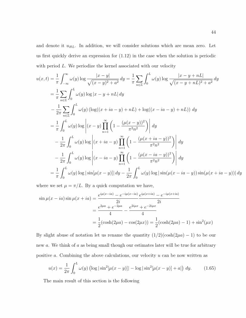
44

and denote it uHL. In addition, we will consider solutions which are mean zero. Let

us first quickly derive an expression for (1.12) in the case when the solution is periodic

with period L. We periodize the kernel associated with our velocity

u(x, t) =1

π

∫ ∞−∞

ω(y) log|x− y|√

(x− y)2 + a2dy =

1

π

∑n∈Z

∫ L

0

ω(y) log|x− y + nL|√

(x− y + nL)2 + a2dy

=1

π

∑n∈Z

∫ L

0

ω(y) log |x− y + nL| dy

− 1

2π

∑n∈Z

∫ L

0

ω(y) (log((x+ ia− y) + nL) + log((x− ia− y) + nL)) dy

=1

π

∫ L

0

ω(y) log

∣∣∣∣∣(x− y)∞∏n=1

(1− (µ(x− y))2

π2n2

)∣∣∣∣∣ dy− 1

2π

∫ L

0

ω(y) log

∣∣∣∣∣(x+ ia− y)∞∏n=1

(1− (µ(x+ ia− y))2

π2n2

)∣∣∣∣∣ dy− 1

2π

∫ L

0

ω(y) log

∣∣∣∣∣(x− ia− y)∞∏n=1

(1− (µ(x− ia− y))2

π2n2

)∣∣∣∣∣ dy=

1

π

∫ L

0

ω(y) log | sin[µ(x− y)]| dy − 1

2π

∫ L

0

ω(y) log | sin(µ(x− ia− y)) sin(µ(x+ ia− y))| dy

where we set µ = π/L. By a quick computation we have,

sinµ(x− ia) sinµ(x+ ia) =eiµ(x−ia) − e−iµ(x−ia)

2i

eiµ(x+ia) − e−iµ(x+ia)

2i

=e2µa + e−2µa

4− e2iµx + e−2iµx

4

=1

2(cosh(2µa)− cos(2µx)) =

1

2(cosh(2µa)− 1) + sin2(µx)

By slight abuse of notation let us rename the quantity (1/2)(cosh(2µa) − 1) to be our

new a. We think of a as being small though our estimates later will be true for arbitrary

positive a. Combining the above calculations, our velocity u can be now written as

u(x) =1

2π

∫ L

0

ω(y)(log | sin2[µ(x− y)]| − log | sin2[µ(x− y)] + a|

)dy. (1.65)

The main result of this section is the following

45

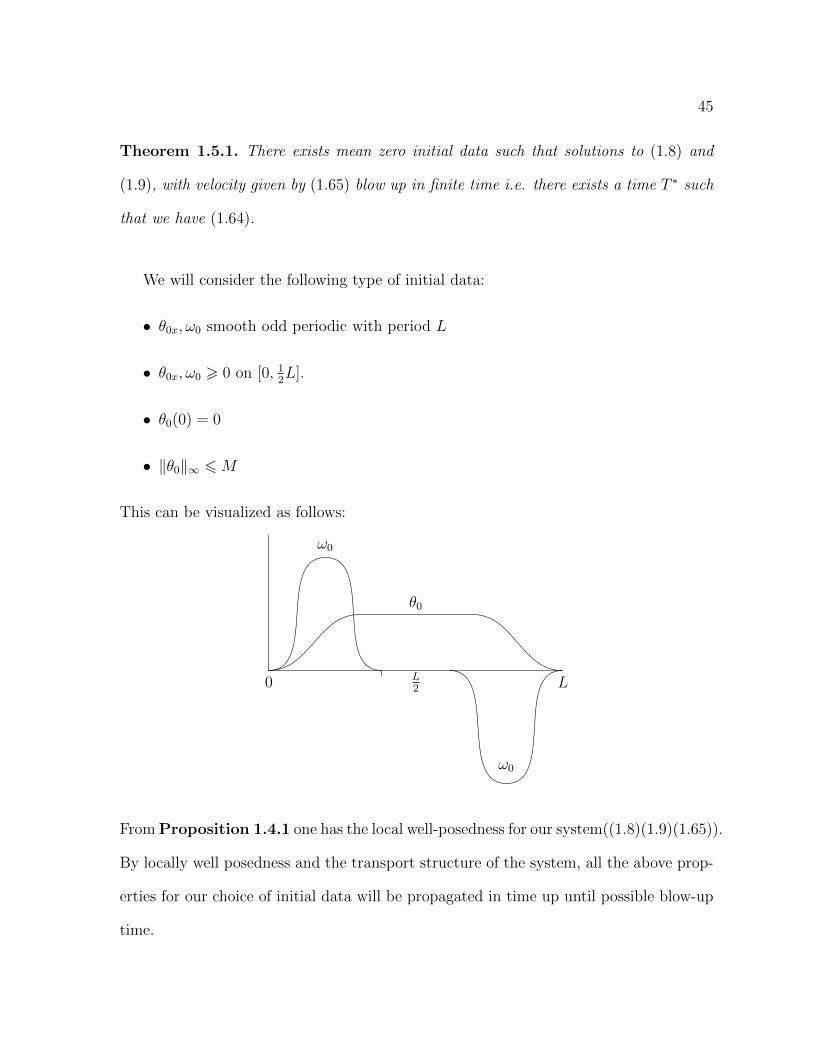
Theorem 1.5.1. There exists mean zero initial data such that solutions to (1.8) and

(1.9), with velocity given by (1.65) blow up in finite time i.e. there exists a time T ∗ such

that we have (1.64).

We will consider the following type of initial data:

• θ0x, ω0 smooth odd periodic with period L

• θ0x, ω0 > 0 on [0, 12L].

• θ0(0) = 0

• ‖θ0‖∞ 6M

This can be visualized as follows:

0

ω0

L2

θ0

ω0

L

From Proposition 1.4.1 one has the local well-posedness for our system((1.8)(1.9)(1.65)).

By locally well posedness and the transport structure of the system, all the above prop-

erties for our choice of initial data will be propagated in time up until possible blow-up

time.

46

The proof of singularity formation will follow by contradiction. This argument is

similar to the blow-up argument in the nonlinear Schrodinger equation ( [38] [85]). The

motivation for the choice of initial data above is the following possible blow-up scenario:

u 6 0 on [0, L/2] and θ will be pushed towards the origin by the flow which also causes

ω to be pushed towards the origin while increasing it’s L∞ norm until there is gradient

blow-up at the origin. Our argument is in a similar spirit to [21] where the authors

consider the quantity ∫ x0

0

ω(x, t)

xdx.

However, we are not able to get an estimate of this quantity. Instead, intuitively the

movement of the bump of ω will lead a fast movement of θ, which may make θx blow

up at the origin. Under this intuition, in the proof of blowup we track the quantity∫ L2

0

θ(x, t) cot(µx)dx.

Using that our initial data is also odd with respect to x = L2

we can write u as

u(x) =1

π

[∫ L/2

0

+

∫ L

L/2

]ω(y)

(log | sin2[µ(x− y)]| − log | sin2[µ(x− y)] + a|

)dy

=1

π

∫ L/2

0

(log

∣∣∣∣sin2 µ(x− y)

sin2 µ(x+ y)

∣∣∣∣+ log

∣∣∣∣sin2 µ(x+ y) + a

sin2 µ(x− y) + a

∣∣∣∣)ω(y) dy

Define

F (x, y, a) =tanµy

tanµx

(log

∣∣∣∣sin2 µ(x− y)

sin2 µ(x+ y)

∣∣∣∣+ log

∣∣∣∣sin2 µ(x+ y) + a

sin2 µ(x− y) + a

∣∣∣∣) (1.66)

and so our corresponding velocity u for the system (1.8) and (1.9) can be written in the

47

following form, which will be useful in the proof

u(x) cot(µx) =1

π

∫ L/2

0

F (x, y, a)ω(y) cot(µy) dy (1.67)

The majority of this section will be devoted to proving properties of F that will allow

for a proof of blow-up analogous to the HL model. These properties are contained in

the following lemma.

Lemma 1.5.2. (a) There exists a positive constant C depending on a such that F (x, y, a) 6

−C < 0 for 0 < x < y < L/2.

(b) For any 0 < y < x < L2

, F (x, y, a) is increasing in x.

(c) For any 0 < x, y < L2

, cot(µy)(∂xF )(x, y, a) + cot(µx)(∂xF )(y, x, a) is positive.

Note that F is not symmetric in x and y. Define

K(x, y) =tanµy

tanµx

(log

∣∣∣∣sinµ(x+ y)

sinµ(x− y)

∣∣∣∣) ,then

F (x, y, a) = −2K(x, y) +tanµy

tanµx

(log

∣∣∣∣sin2 µ(x+ y) + a

sin2 µ(x− y) + a

∣∣∣∣) . (1.68)

The term K(x, y) arises from the HL model and we view as the main contributor

from F in regards to blow-up. In order to show lemma 1.5.2, we need the following

technical lemma for K(x, y):

Lemma 1.5.3. For simplicity, let’s write K(x, y) in the following form:

K(x, y) = s log

∣∣∣∣s+ 1

s− 1

∣∣∣∣ , with s =tan(µy)

tan(µx). (1.69)

Then it has the following properties:

48

(a) K(x, y) > 0 for all x, y ∈ (0, 12L) with x 6= y

(b) K(x, y) > 2 and Kx(x, y) > 0 for all 0 < x < y < 12L

(c) K(x, y) > 2s2 and Kx(x, y) 6 0 for all 0 < y < x < 12L

The detailed proof of lemma 1.5.3 can be found in [12].

Proof of Lemma (1.5.2)(a). First, it is easy to see that F is non-positive. Indeed∣∣∣∣sin2 µ(x− y)

sin2 µ(x+ y)

∣∣∣∣ ∣∣∣∣sin2 µ(x+ y) + a

sin2 µ(x− y) + a

∣∣∣∣ =

∣∣∣∣∣1 + asin2 µ(x+y)

1 + asin2 µ(x−y)

∣∣∣∣∣ 6 1 (1.70)

because sin2 µ(x− y) 6 sin2 µ(x+ y).

For the better upper bound, we first consider the region 0 < x < y < L/4. For the

region L/4 < x < y < L/2, if we take x∗ = L2− x, y∗ = L

2− y, then 0 < y∗ < x∗ < L/4,

this means the argument for this region would be the same as the region 0 < x < y < L/4

by changing the name of the variables. Hence, let us only consider the previous region.

We divide our estimate into 4 separate cases. Let a∗ = mina, 116.

Case 1:√a∗

πL =

√a∗

µ< x < y < L/4

In this domain we have sinµy > sinµx >sin(π

4)

π4µx > 1√

2µx > 1√

2

√a∗, cosµx >

cosµy > 1√2, hence

sin2 µ(x− y) = sin2 µ(x+ y)− 4 sinµx sinµy cosµx cosµy < sin2 µ(x+ y)− a∗,

so

F (x, y, a) 6 log

∣∣∣∣sin2 µ(x− y)

sin2 µ(x+ y)

∣∣∣∣+ log

∣∣∣∣sin2 µ(x+ y) + a∗

sin2 µ(x− y) + a∗

∣∣∣∣ = log

∣∣∣∣∣1 + a∗

sin2 µ(x+y)

1 + a∗

sin2 µ(x−y)

∣∣∣∣∣ (1.71)

6 log

∣∣∣∣∣ 1 + a∗

sin2 µ(x+y)

1 + a∗

sin2 µ(x+y)−a∗

∣∣∣∣∣ 6 −C0(a) < 0

(1.72)

49

where C0(a) is a positive constant independent of x, y. In the last step we use the fact

that the function

(1 +

a∗

z

)(1 +

a∗

z − a∗

)−1

= 1− (a∗)2

z2is increasing in z for a∗ < z < 1

and fixed a∗.

Case 2: 0 < x < y <√a∗

µ< L/4

From lemma 1.5.3 (b), we know

−4 > −2K(x, y) =tanµy

tanµxlog

∣∣∣∣tanµy + tanµx

tanµy − tanµx

∣∣∣∣2 =tanµy

tanµxlog

∣∣∣∣sin2 µ(x− y)

sin2 µ(x+ y)

∣∣∣∣ .so if we can show the contribution from the other part of F (x, y, a) is bounded above by

some constant less than 4, we are done. Expanding, we have that second term in (1.68)

is equal to

tanµy

tanµxlog

∣∣∣∣sin2 µx cos2 µy + 2 sinµx cosµy sinµy cosµx+ sin2 µy cos2 µx+ a

sin2 µx cos2 µy − 2 sinµx cosµy sinµy cosµx+ sin2 µy cos2 µx+ a

∣∣∣∣ . (1.73)

Since 0 < y <√a∗

µ6√aµ

, we know sin2 µy cos2 µx < sin2√a · 1 < a. Then we have that

(1.73) is bounded above by

tanµy

tanµxlog

∣∣∣∣sin2 µx cos2 µy + 2 sinµx cosµy sinµy cosµx+ 2 sin2 µy cos2 µx

sin2 µx cos2 µy − 2 sinµx cosµy sinµy cosµx+ 2 sin2 µy cos2 µx

∣∣∣∣ = s log

∣∣∣∣2s+ 1s

+ 2

2s+ 1s− 2

∣∣∣∣(1.74)

where s =tanµy

tanµx. As a function of s, by direct calculation we find the derivative of the

right hand side of (1.74) is

4s− 8s3

1 + 4s4+ log

∣∣∣∣2s+ 1s

+ 2

2s+ 1s− 2

∣∣∣∣ . (1.75)

By taking the derivative of (1.75), we find the second derivative of (1.74) is

−8(4s4 + 4s2 − 1)

(4s4 + 1)2,

50

which is negative for s > 1. And we know

lims→∞

4s− 8s3

1 + 4s4+ log

∣∣∣∣2s+ 1s

+ 2

2s+ 1s− 2

∣∣∣∣ = 0

which means the right hand side of (1.74) is increasing in s for s > 1 and

lims→∞

s log

∣∣∣∣2s+ 1s

+ 2

2s+ 1s− 2

∣∣∣∣ = 2.

Case 3:√a∗

2µ< x <

√a∗

µ< y < L/4

In this case, because we know x is away from 0, s =tanµy

tanµx6 C1(a) for some constant

depending on a. Also, cos2 µy sin2 µx 6 1 · sin2√a 6 a. Then (1.73) is bounded above

by

s log

∣∣∣∣s+ 2 + 2s

s− 2 + 2s

∣∣∣∣ . (1.76)

Similarly to the previous case, the second derivative of (1.76) is negative for s > 1 and

the limit of the first derivative of (1.76) as s goes to infinity is zero, which means (1.76)

monotonically increases to 4 as s → ∞ for s > 1. However, since s is bounded above,

the expression above can be bounded by some constant C2(a) which is strictly less than

4.

Case 4: 0 < x <√a∗

2µ<√a∗

µ< y < L/4

On the set A = (x, y) : 0 6 x 6√a∗

2µ,√a∗

µ6 y 6 L/4, F (x, y, a) is a continuous

negative function (since |x− y| has a positive lower bound and points where x = 0 are

removable singularities). Since F 6= 0 on A and A is compact, F achieves a maximum

C3(a) which is strictly less than 0.

This completes the analysis for the region 0 < x < y < L/4. Now, we are left the

domain 0 < x < L/4 < y < L/2.

51

This case is simpler and the analysis is divided in the following two cases. First,

suppose 0 < L/8 < x < L/4 < y < 3L/8 < L/4 Then 3π8< µ(x + y) < 5π

8and

0 < µ(y − x) < π4

so there exists ε > 0 such that sin2 µ(x + y) > 12

+ ε. However,

sin2 µ(x− y) < 12. From this, we get sin2 µ(x+ y)− sin2 µ(x− y) > ε∗ for some constant

ε∗, which means (1.71) follows if we replace the a∗ by ε∗. Then we get the desired

estimate. If x and y are not in this region, there exists a constant c > 0 such that

y−x > c > 0, then again by the same argument as in the Case 4 and we get the desired

inequality.

This completes the proof of (a).

Proof of 1.5.2(b). We compute directly and get

cot(µy)(∂xF )(x, y, a) = −µ csc2(µx)

(log

(sin2 µ(x− y)

sin2 µ(x+ y)

)+ log

(sin2 µ(x+ y) + a

sin2 µ(x− y) + a

))+ µ cot(µx)

[2 sinµ(x− y) cosµ(x− y)

sin2 µ(x− y)− 2 sinµ(x− y) cosµ(x− y)

sin2 µ(x− y) + a

]− µ cot(µx)

[2 sinµ(x+ y) cosµ(x+ y)

sin2 µ(x+ y)− 2 sinµ(x+ y) cosµ(x+ y)

sin2 µ(x+ y) + a

]= −µ csc2(µx)

(log

(sin2 µ(x− y)

sin2 µ(x+ y)

)+ log

(sin2 µ(x+ y) + a

sin2 µ(x− y) + a

))+ µ cot(µx)

[2a sinµ(x− y) cosµ(x− y)

sin2 µ(x− y)(sin2 µ(x− y) + a)− 2a sinµ(x+ y) cosµ(x+ y)

sin2 µ(x+ y)(sin2 µ(x+ y) + a)

]= I + II.

For I, by the same calculation as (1.70), we know it is positive. For II, when x > y,

can be expressed as

cot(µx)(f(x− y)− f(x+ y)),

52

where f(t) = cos(µt)

sin(µt)(sin2(µt)+a). It is easy to see that whenever 0 < y < x < L

2, cosµ(x−

y) > cosµ(x + y), sinµ(x − y) 6 sinµ(x + y). This means f(x − y) > f(x + y), which

also means II > 0. This completes the proof of (b).

Proof of 1.5.2(c). Now, for the final part of the lemma. First of all, we set

G(x, y, a) = cot(µy)(∂xF )(x, y, a) + cot(µx)(∂xF )(y, x, a)

= −µ(csc2(µx) + csc2(µy))

[log

(sin2 µ(x− y)

sin2 µ(x+ y)

)+ log

(sin2 µ(x+ y) + a

sin2 µ(x− y) + a

)]+ µ(cot(µx)− cot(µy))

2a sinµ(x− y) cosµ(x− y)

sin2 µ(x− y)(sin2 µ(x− y) + a)

− µ(cot(µx) + cot(µy))2 sinµ(x+ y) cosµ(x+ y)

sin2 µ(x+ y)(sin2 µ(x+ y) + a).

= −µ(cot2(µx) + cot2(µy) + 2)

[log

(sin2 µ(x− y)

sin2 µ(x+ y)

)+ log

(sin2 µ(x+ y) + a

sin2 µ(x− y) + a

)]− µ 2a cosµ(x− y)

(sin2 µ(x− y) + a) sin(µx) sin(µy)− µ 2a cosµ(x+ y)

(sin2 µ(x+ y) + a) sin(µx) sin(µy)

= −µ(cot2(µx) + cot2(µy) + 2)

[log

(sin2 µ(x− y)

sin2 µ(x+ y)

)+ log

(sin2 µ(x+ y) + a

sin2 µ(x− y) + a

)]− 2µ cot(µx) cot(µy)

[a

sin2 µ(x− y) + a+

a

sin2 µ(x+ y) + a

]− 2µ

[a

sin2 µ(x− y) + a− a

sin2 µ(x+ y) + a

]Now our aim is to prove the positivity of G(x, y, a). Notice that when a = 0, G(x, y, a) =

0, as a consequence, to prove the positivity of G(x, y, a), the only thing we need to show

53

is that this function is increasing in a for any x, y in the domain. On the other hand,

1

µ∂aG(x, y, a) = (cot2(µx) + cot2(µy) + 2)

[1

sin2 µ(x− y) + a− 1

sin2 µ(x+ y) + a

]− 2 cot(µx) cot(µy)

[sin2 µ(x− y)

(sin2 µ(x− y) + a)2+

sin2 µ(x+ y)

(sin2 µ(x− y) + a)2

]− 2[

sin2 µ(x− y)

(sin2 µ(x− y) + a)2− sin2 µ(x+ y)

(sin2 µ(x+ y) + a)2]

= (cot2(µx) + cot2(µy) + 2)sin2 µ(x− y)− sin2 µ(x+ y)

(sin2 µ(x− y) + a)(sin2 µ(x+ y) + a)

− 2 cot(µx) cot(µy)

[sin2 µ(x− y)

(sin2 µ(x− y) + a)2+

sin2 µ(x+ y)

(sin2 µ(x− y) + a)2

]− 2

[sin2 µ(x− y)

(sin2 µ(x− y) + a)2− sin2 µ(x+ y)

(sin2 µ(x+ y) + a)2

].

Therefore,

1

µ((sin2 µ(x− y) + a)(sin2 µ(x+ y) + a))2∂aG(x, y, a)

= (cot2(µx) + cot2(µy) + 2)(sin2 µ(x+ y)− sin2 µ(x− y))(sin2 µ(x− y) + a)(sin2 µ(x+ y) + a)

− 2 cot(µx) cot(µy)[sin2 µ(x− y)(sin2 µ(x+ y) + a)2 + sin2 µ(x+ y)(sin2 µ(x− y) + a)2

]− 2

[sin2 µ(x− y)(sin2 µ(x+ y) + a)2 − sin2 µ(x+ y)(sin2 µ(x− y) + a)2

].

It is easy to see this is a quadratic polynomial in a of the form A2x2 +A1x+A0. We will

explicitly compute A2, A1, and A0 and show each term is non-negative. For the second

54

order term we get

A2 = (cot2(µx) + cot2(µy) + 2)(sin2 µ(x− y)− sin2 µ(x+ y))

− 2 cot(µx) cot(µy)[sin2 µ(x− y) + sin2 µ(x+ y)]

− 2[sin2 µ(x− y)− sin2 µ(x+ y)].

= (cot2(µx) + cot2(µy))(sin2 µ(x+ y)− sin2 µ(x− y))

− 2 cot(µx) cot(µy)[sin2 µ(x− y) + sin2 µ(x+ y)].

This means

tan(µx) tan(µy)A2 =(tan(µx)

tan(µy)+

tan(µy)

tan(µx))(sin2 µ(x+ y)− sin2 µ(x− y))

− 2[sin2 µ(x− y) + sin2 µ(x+ y)].

If we set tan(µx)tan(µy)

= s, wel have

tan(µx) tan(µy)

cos(µy) cos(µx) sin(µy) sin(µx)A2 = (s+

1

s) · 4− 2[2 · (s+

1

s)] = 0.

This means as long as 0 < x, y < L2, A2 = 0. Similarly, for coefficient of the first order

term A1, we have

A1 = (cot2(µx) + cot2(µy) + 2)(sin2 µ(x+ y)− sin2 µ(x− y))(sin2 µ(x+ y) + sin2 µ(x− y))

− 2 cot(µx) cot(µy)[2 sin2 µ(x− y) sin2 µ(x+ y) + 2 sin2 µ(x+ y) sin2 µ(x− y)]

− 2[2 sin2 µ(x− y) sin2 µ(x+ y)− 2 sin2 µ(x+ y) sin2 µ(x− y)]

> (cot2(µx) + cot2(µy))[sin4 µ(x+ y)− sin4 µ(x− y)]

− 8 cot(µx) cot(µy)[sin2 µ(x− y) sin2 µ(x+ y)].

Again, by setting tan(µx)tan(µy)

= s, we get

tan(µx) tan(µy)

cos(µx) cos(µy) sin(µx) sin(µy)A1 > (s+

1

s) · 4 · 2(s+

1

s)− 8(s+

1

s− 2)(s+

1

s+ 2) > 32.

55

Lastly, for the coefficient of the constant term A0, we have

A0 = (cot2(µx) + cot2(µy) + 2)(sin2 µ(x+ y)− sin2 µ(x− y)) sin2 µ(x+ y) sin2 µ(x− y)

− 2 cot(µx) cot(µy)[sin2 µ(x− y) sin2 µ(x+ y)(sin2 µ(x+ y) + sin2 µ(x− y))]

− 2 sin2 µ(x− y) sin2 µ(x+ y)[sin2 µ(x+ y)− sin2 µ(x− y)]

= (cot2(µx) + cot2(µy))(sin2 µ(x+ y)− sin2 µ(x− y)) sin2 µ(x+ y) sin2 µ(x− y)

− 2 cot(µx) cot(µy) sin2 µ(x− y) sin2 µ(x+ y)[sin2 µ(x+ y) + sin2 µ(x− y)].

For x = y, A0 = 0. Otherwise, again by setting s = tan(µx)tan(µy)

after computation we have

tan(µx) tan(µy)

sin2 µ(x− y) sin2 µ(x+ y) cos(µx) cos(µy) sin(µx) sin(µy)A0 = (s+

1

s)·4−2·(2s+2

s) = 0.

In all, we have ∂aG(x, y, a) > 0 for 0 < x, y < L2. This completes the proof.

Remark 1.5.4. One may notice that when a→∞, 1µG(x, y, a) tends to

−(cot2(µx) + cot2(µy) + 2)

[log

(sin2 µ(x− y)

sin2 µ(x+ y)

)]− 4 cot(µx) cot(µy). (1.77)

The positivity of this quantity is also proved by lemma 4.2 in [12], in which the authors

use technical trigonometric inequalities. Our proof of the above lemma provides another

approach to estimating this quantity.

With these lemmas at our disposal, we are ready to prove finite-time blow up.

Proof of Theorem 1.5.1.

Suppose we have a global smooth solution. We will show blow up of the following

quantity:

I(t) :=

∫ L/2

0

θ(x, t) cot(µx) dx.

56

thereby arriving at a contradiction since

|I(t)| 6 C‖θ0x‖L∞ exp

(∫ t

0

‖ux(·, s)‖L∞ ds).

If I were to become infinite in finite time, we would be able to use Beale-Kato-Majda

type condition for the system as stated in equation (1.64) from which we can conclude

blow-up. We first compute the derivative of I(t):

d

dtI(t) = − 1

π

∫ L/2

0

θx(x)

∫ L/2

0

ω(y) cot(µy)F (x, y, a) dy dx.

By the negativity of F and part (a) of the lemma, the expression above is bounded below

by

C

π

∫ L/2

0

θx(x)

∫ L/2

x

ω(y) cot(µy) dy dx =C

π

∫ L/2

0

θ(x)ω(x) cot(µx) dx := CJ(t),

where J(t) = 2π

∫ L/20

θ(x)ω(x) cot(µx) dx. Then,

d

dt(CJ(t)) =

C

π

∫ L/2

0

θ(x)ω(x) (u(x) cot(µx))x dx+Cµ

2π

∫ L/2

0

θ2(x) csc2(µx) dx (1.78)

By Cauchy-Schwarz inequality, the second integral is bounded below by CL2 I(t)2 for some

constant C. The first integral is given by

C

π

∫ L/2

0

θy(y)

[∫ L/2

y

ω(x) (u(x) cot(µx))x dx

]dy (1.79)

Observe that since θ is non-decreasing on [0, L/2], the expression (1.79) is positive if

we can show the integral in the brackets is positive as well. This is our next task. For

x, y ∈ [0, 12L], ω(x) can be decomposed as

ω(x) = ω(x)χ[0,y](x) + ω(x)χ[y, 12L](x) =: ω`(x) + ωr(x).

57

Then we can decompose the integral:∫ L/2

y

ω(x)[u(x) cot(µx)]x dx =1

π

∫ L/2

0

ωr(x)

∫ L/2

0

ω`(y) cot(µy)(∂xF )(x, y, a) dy dx

+1

π

∫ L/2

0

ωr(x)

∫ L/2

0

ωr(y) cot(µy)(∂xF )(x, y, a) dy dx

By positivity of ω on [0, 12L] and part (b) of the key lemma, the first integral is positive.

By using symmetry, the second integral is equal to

1

2π

∫ L/2

0

∫ L/2

0

ωr(x)ωr(y)G(x, y, a) dy dx

where G(x, y, a) = cot(µy)(∂xF )(x, y, a) + cot(µx)(∂xF )(y, x, a). However, by part (c)

of the lemma, this is positive. Together with (1.78) and (1.79) we have:

d2

dt2I > CI2, (1.80)

for some constant C. To close the proof, we only need the following lemma:

Lemma 1.5.5. Suppose I(t) solve the following initial value problem:

d

dtI(t) > C

∫ t

0

I2(s)ds, I(0) = I0. (1.81)

Then there exists T = T (C, I0) so that limt→T I(t) =∞.

Moreover, for fixed C and any ε > 0, there is an A > 0, so that for any I0 > A, the

blow up time T < ε.

The proof of this lemma is straightforward, and one can also find the proof in [12].

58

1.6 Perturbation

In this section, we consider our system (1.8) and (1.9) but with a Biot-Savart which is

a perturbation of the Hou-Lou kernel. We will work with periodic solutions with period

L. The velocity u is given by the following choice of Biot-Savart Law

u(x) =1

π

∫ L

0

(log | sin[µ(x− y)]|+ f(x, y))ω(y) dy, µ := π/L (1.82)

:= uHL(x) + uf (x) (1.83)

where f is a smooth function whose precise properties we will specify later. We view f

as a perturbation and we will show solutions to the system (1.8) and (1.9) with (1.82)

can still blow-up in finite time. As with the previous system (1.8), (1.9), (1.12), we still

have a local-well-posedness result akin to Proposition (1.4.1) holds here. In particular,

if T ∗ is a maximal time of existence of a solution then we must have

limtT ∗

∫ t

0

‖ux(·, τ)‖L∞ dτ =∞ (1.84)

We show such a time can exist below.

Theorem 1.6.1. Let f ∈ C2(R2), periodic with period L such that f(x, y) = f(−x,−y)

for all x, y. Then there exists initial data ω0, θ0 such that solutions of (1.8) and (1.9),

with velocity given by (1.82), blow up in finite time. Again, that means there exists a

time T ∗ such that we have (1.84).

We will consider the following type of initial data:

• θ0x, ω0 smooth odd periodic with period L

• θ0x, ω0 > 0 on [0, 12L].

59

• θ0(0) = 0

• (supp θ0x ∪ suppω0) ∩ [0, 12L] ⊂ [0, ε]

• ‖θ0‖∞ 6M

We will make the choice of specific ε below and unless stated otherwise, ε will always

refer to the ε defined in the way above. Observe that by the assumptions, ω0 and θ0x

are also odd with respect to 12L. By the following lemma 1.6.4, we can choose ε such

that the mass of ω near the origin gets closer to the origin leading to a scenario where

blow-up can be achieved.

Remark 1.6.2. With the choice of f(x, y) = log√

sin2 µ(x− y) + a, we have the kernel

from the previous section. However, in the previous section, we proved blow-up for a

larger class of initial data.

Remark 1.6.3. Comparing with the construction in the previous section, one can find

that the initial condition for the blow up of general pertubation is more restrictive, we

require small-supported initial data in order to achieve singularity formation.

Lemma 1.6.4. With the initial data ω0 and θ0 as given above, we can choose ε1 small

such that for ε < ε1, u(x) < 0 for x 6 ε where u is defined as (1.82).

Proof. By periodicity and support property of ω,

u(x) =1

π

∫ L/2

0

(log

∣∣∣∣tan(µx)− tan(µy)

tan(µx) + tan(µy)

∣∣∣∣+ f(x, y)− f(x,−y)

)ω(y) dy

=1

π

∫ ε

0

(log

∣∣∣∣tan(µx)− tan(µy)

tan(µx) + tan(µy)

∣∣∣∣+ f(x, y)− f(x,−y)

)ω(y) dy.

60

By the mean value theorem, for 0 6 y 6 ε, |f(x, y) − f(x,−y)| 6 2ε‖f‖C1 . By the

singularity of the HL kernel when x = y = 0, we can choose ε1 such that the expression

in the parentheses is negative for 0 < x, y 6 ε.

We will also need the following lemma controlling the integral of ω over half the period.

Lemma 1.6.5. There exists ε2 > 0 such that for ε < ε2, with ω0 and θ0 as chosen above,

solutions of (1.8), (1.9), (1.82) satisfy∫ L/2

0

ω(y, t) dy 6Mt.

Proof. Integrating both sides of (1.8) and integrating by parts we get∫ L/2

0

ωt(y, t) dy =

∫ L/2

0

ux(y)ω(y, t) dy +

∫ L/2

0

θx(y, t) dy 6M +

∫ L/2

0

ux(y)ω(y, t) dy

If we can show the remaining integral on the right is negative, we are done. The integral

can be written as

1

π

∫ L/2

0

∫ L/2

0

(cot[µ(x− y)]− cot[µ(x+ y)] + fx(x, y)− fx(x,−y))ω(x)ω(y) dy dx

By symmetry, the integral with cot[µ(x− y)] is 0 and using the support property of ω,

the above line is equal to

1

π

∫ ε

0

∫ ε

0

(− cot[µ(x+ y)] + fx(x, y)− fx(x,−y))ω(x)ω(y) dy dx

Since f is smooth and ω is positive, we can make ε2 smaller so that the expression in

the parentheses above in the integrand is negative.

Now, so we can take advantage of our lemmas, we choose ε = minε1, ε2 for the support

of our initial data.

61

Proof of Theorem 1.6.1. Throughout, C(f) will be a positive constant that only depends

on f and not ω0. We will show that

I(t) :=

∫ L/2

0

θ(x, t) cot(µx) dx (1.85)

must blow-up. Taking time derivative of I and using lemma 1.5.3, we get

d

dtI(t) = −

∫ L/2

0

u(x)θx(x) cot(µx) dx

=1

π

∫ L/2

0

θx(x)

∫ L/2

0

ω(y) cot(µy)K(x, y) dy dx

+

∫ L/2

0

θx(x) (uf (x) cot(µx)) dx > J(t) +

∫ L/2

0

θx(x) (uf (x) cot(µx)) dx

where, using the same notation as before,

J(t) =2

π

∫ L/2

0

θ(x)ω(x) cot(µx) dx

Now, we would like to bound the extra term arising because of f . Since f is smooth

and ω is supported near the origin,

|u(x) cot(µx)| =∣∣∣∣∫ ε

0

[cot(µx)(f(x, y)− f(x,−y))]ω(y) dy

∣∣∣∣ 6 C(f) ·

(∫ L/2

0

ω(y)dy

).

Therefore, we have

d

dtI(t) > J(t)− C(f)M

(∫ L/2

0

ω(y)dy

)> J(t)− C(f)M2t (1.86)

Now, we derive a differential inequality for J(t).

d

dtJ(t) =

2

π

∫ L/2

0

−(θ(x)ω(x))xu(x) cot(µx) + θx(x)θ(x) cot(µx) dx

=2

π

∫ L/2

0

θ(x)ω(x)(u(x) cot(µx))x dx+µ

π

∫ L/2

0

θ2(x) csc2(µx) dx

62

As before, by Cauchy-Schwarz inequality the second integral is bounded below by

2

L2I(t)2. We split the first integral into two parts:

2

π

∫ L/2

0

θ(x)ω(x)(uHL(x) cot(µx))x dx+2

π

∫ L/2

0

θ(x)ω(x)(uf (x) cot(µx))x dx.

By the arguments in the proof of theorem 1.5.1, the first integral is positive. For the

second integral, we integrate by parts and get

2

π

∫ L/2

0

θy(y)

[∫ L/2

y

ω(x)(uf (x) cot(µx))x dx

]dy (1.87)

Using the smoothness and boundedness of f ,

|∂x(uf (x) cot(µx))| =∣∣∣∣∫ ε

0

∂x [cot(µx)(f(x, y)− f(x,−y))]ω(y) dy

∣∣∣∣ (1.88)

Now let h(x, y) = cot(µx)(f(x, y)− f(x,−y)). Then it is easy to see that h ∈ C1 when

f ∈ C2, which also means ∂xh(x, y) is bounded above. This mean the right hand side of

(1.88) can be bounded above by

6 C(f) ·

(∫ L/2

0

ω(y)dy

).

Inserting this estimate into (1.87), we get that it is bounded below by

−C(f)M

(∫ L/2

0

ω(y)dy

)2

.

Putting things together, we get

d

dtJ(t) >

2

L2I(t)2 − C(f)M

(∫ L/2

0

ω(y)dy

)2

>2

L2I(t)2 − C(f)M3t2 (1.89)

Now, we will show the differential inequalities we have shown will lead to blow-up. By

(1.86) and (1.89) we have

d

dtI(t) >

2

L2

∫ t

0

I2(s) ds+ J(0)− c(f)M2t− C(f)M3 t3

3

>2

L2

∫ t

0

I2(s) ds− c(f)M2t− C(f)M3 t3

3

(1.90)

63

We claim that one can choose I(0) large enough so that the effect of the negative terms

is minimized. By a rather crude estimate we have

d

dtI(t) > −c(f)M2t− C(f)M3 t

3

3.

After integration, this implies

I(t) > I(0)− C(f)M2

(t2

2+M

t4

12

). (1.91)

Now fix a time, say 1, and we’ll show I(0) can be chosen large enough so that I(t) blows

up before time 1. We first choose I(0) > C(f)M2(

12

+M 112

), then for t < 1,

1

L2

∫ t

0

I2(s) ds >t

L2

[I(0)− C(f)M2

(1

2+M

12

)]2

Choose I(0) such that

I(0) > C(f)M2

(1

2+M

12

)+ L

√c(f)M2 + C(f)

M3

3

Then, for 0 < t < 1, with this choice of I(0), using (1.90)

d

dtI(t) >

1

L2

∫ t

0

I(s)2 ds+ t

(c(f)M2 + C(f)

M3

3

)− c(f)M2t− C(f)M3 t

3

3

>1

L2

∫ t

0

I(s)2 ds

By perhaps making I(0) a little larger, if needed, we can show I(t) becomes infinite

before time 1 by lemma 1.5.5.

64

Chapter 2

Mixing by Fluid Flow

2.1 Introduction

In the previous chapter, we discuss the possible singularity formation of nonlinear nonlo-

cal differential equations. In this chapter, we consider the problem in the other direction,

which is how to regularize the solution to a differential equation. We finally show that

the optimal mixing flow are able to prevent the singularity formation. Hence, in this

chapter, we start from studying the term “mixing”, then try to take advantage of it.

2.1.1 Mixing

The mixing of tracer particles by fluid flows is ubiquitous in nature, and have applica-

tions ranging from weather forecasting to food processing. An important question that

has attracted attention recently is to study “how well” tracers can be mixed under a

constraint on the advecting velocity field, and what is the optimal choice of the “best

mixing” velocity field (see [83] for a recent review).

Our aim in section 2.2 is to study how well passive tracers can be mixed under an

enstrophy constraint on the advecting fluid. By passive, we mean that the tracers pro-

vide no feedback to the advecting velocity field. Further, we assume that diffusion of the

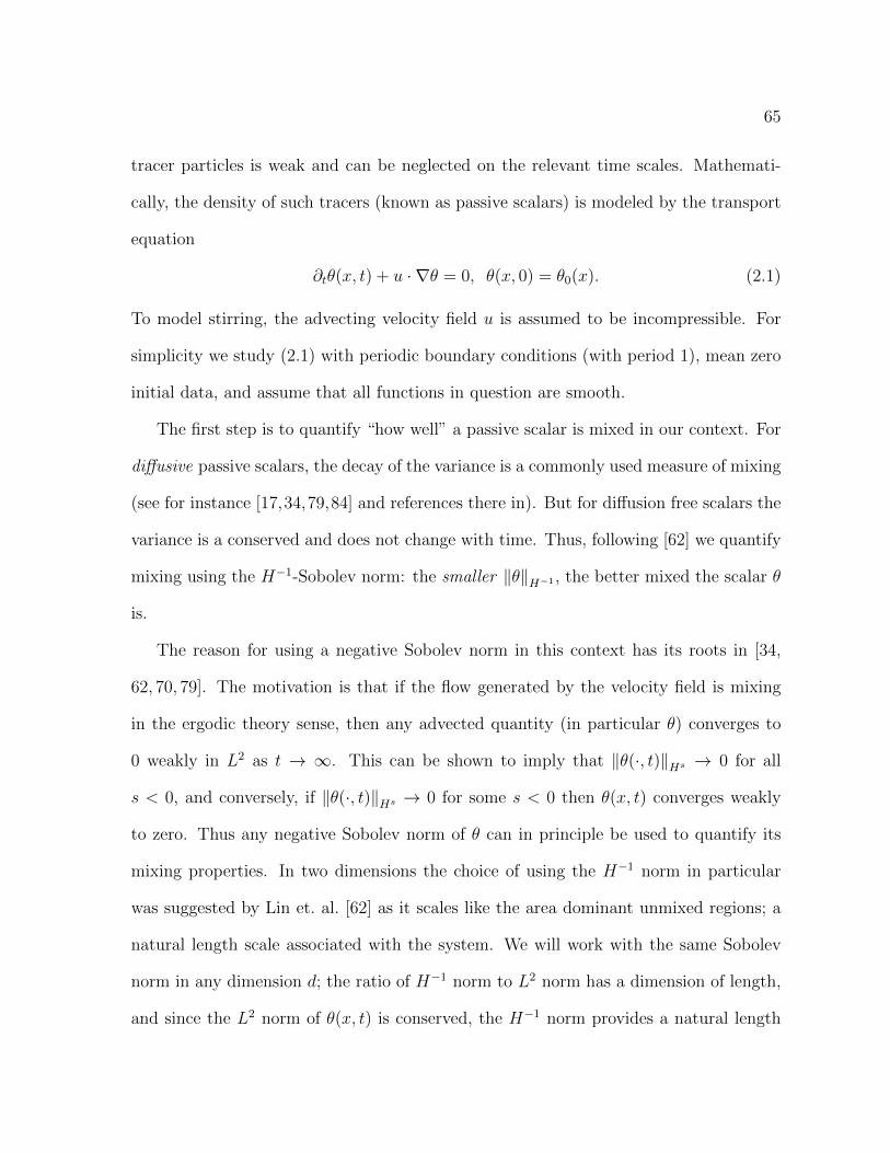
65

tracer particles is weak and can be neglected on the relevant time scales. Mathemati-

cally, the density of such tracers (known as passive scalars) is modeled by the transport

equation

∂tθ(x, t) + u · ∇θ = 0, θ(x, 0) = θ0(x). (2.1)

To model stirring, the advecting velocity field u is assumed to be incompressible. For

simplicity we study (2.1) with periodic boundary conditions (with period 1), mean zero

initial data, and assume that all functions in question are smooth.

The first step is to quantify “how well” a passive scalar is mixed in our context. For

diffusive passive scalars, the decay of the variance is a commonly used measure of mixing

(see for instance [17,34,79,84] and references there in). But for diffusion free scalars the

variance is a conserved and does not change with time. Thus, following [62] we quantify

mixing using the H−1-Sobolev norm: the smaller ‖θ‖H−1 , the better mixed the scalar θ

is.

The reason for using a negative Sobolev norm in this context has its roots in [34,

62, 70, 79]. The motivation is that if the flow generated by the velocity field is mixing

in the ergodic theory sense, then any advected quantity (in particular θ) converges to

0 weakly in L2 as t → ∞. This can be shown to imply that ‖θ(·, t)‖Hs → 0 for all

s < 0, and conversely, if ‖θ(·, t)‖Hs → 0 for some s < 0 then θ(x, t) converges weakly

to zero. Thus any negative Sobolev norm of θ can in principle be used to quantify its

mixing properties. In two dimensions the choice of using the H−1 norm in particular

was suggested by Lin et. al. [62] as it scales like the area dominant unmixed regions; a

natural length scale associated with the system. We will work with the same Sobolev

norm in any dimension d; the ratio of H−1 norm to L2 norm has a dimension of length,

and since the L2 norm of θ(x, t) is conserved, the H−1 norm provides a natural length

66

scale associated with the mixing process.

The questions we study in section 2.2 are motivated by recent work of Lin et. al. [62].

In [62], the authors address two questions on the two dimensional torus:

• The time decay of ‖θ(t)‖H−1 , given the fixed energy constraint ‖u(t)‖L2 = U .

• The time decay of ‖θ(t)‖H−1 given a fixed enstrophy constraint of the form ‖∇u(t)‖L2 =

F .

In the first case the authors prove a lower bound for ‖θ(·, t)‖H−1(T2) that is linear in

t, with negative slope. This suggests that it may be possible to “mix perfectly in finite

time”; namely choose u in a manner that drives ‖θ(·, t)‖H−1 to zero in finite time. This

was followed by an explicit example in [66] exhibiting finite time perfect mixing, under

a finite energy constraint. This example uses an elegant “slice and dice” construction,

which requires the advecting velocity field to develop finer and finer scales. Thus, while

their example maintains a fixed energy constraint, the enstrophy (‖∇u‖L2) explodes.

Together with the numerical analysis in [62, 66] this suggests that finite time perfect

mixing by an enstrophy constrained incompressible flow might be impossible. Our main

theorem in section 2.2 settles this affirmatively. A simplified version of the main theorem

of section 2.2 can be stated as follows:

Theorem 2.1.1. Let u be any incompressible flow satisfies ‖∇u(t)‖L2 6 F for all t. Let

θ be the solution to (2.1), then ‖θ(·, t)‖H−1 > c1 exp(−Ct) for some constants c1 and C,

where the decay rate C only depends on ‖θ0‖L∞, F and the size of super level set of θ0.

67

2.1.2 Preventing blow-up by mixing

After the previous project, there are two questions one may ask: Is this exponential

lower bound sharp? Can this give some insight into the process of mixing be useful in

other PDE models of natural processes?

For the first question, the numerical experiments in [48] suggest this lower bound

should be sharp. Recently, in [88], Yao Yao and Andrej Zlatos proved that the ex-

ponential lower bound is sharp by constructing a family of specific flows. A different

construction leading to similar results was given in [2].

The second question is more open ended and so a bit harder to answer. In section

2.3, we study the role of mixing in systems where chemotaxis is present.

Chemotaxis is ubiquitous in biology and ecology. This term is used to describe motion

where cells or species sense and attempt to move towards higher (or lower) concentration

of some chemical. The first mathematically rigorous studies of chemotaxis effects have

been by Patlak [76] and Keller-Segel [51], [52]. The latter work involved derivation and

first analysis of Keller-Segel system, the most studied model of chemotaxis. Keller-Segel

equation describes a population of bacteria or mold that secrete a chemical and are

attracted by it. In one version of the simplified parabolic-elliptic form, this equation can

be written in Rd as (see e.g. [77])

∂tρ−∆ρ+∇ · (ρ∇(−∆)−1ρ) = 0, ρ(x, 0) = ρ0(x). (2.2)

The last term on the left hand side describes attraction of ρ by the chemical whose

concentration is given by c(x, t) = (−∆)−1ρ(x, t). The literature on the Keller-Segel

equation is enormous. It is known that in dimensions larger than one, solutions to (2.2)

can concentrate finite mass in a measure zero region and so blow up in finite time. We

68

refer to [77], [40], and [41] for more details and further references.

Typically, chemotactic processes take place in fluid, and often the agents involved in

chemotaxis are also advected by the ambient flow. Some of the examples involve mono-

cytes using chemokine signalling to concentrate at a source of infection (see e.g. [29,82]),

sperm and eggs of marine animals practicing broadcast spawning in the ocean (see

e.g. [14,72]), and other numerous instances in biology and ecology. Our goal in this sec-

tion is to study the possible effects resulting from interaction of chemotactic and fluid

transport processes. Of particular interest to us is the possibility of suppression of finite

time blow up due to the mixing effect of fluid flow. The problem of chemotaxis in fluid

flow has been studied before; for example, in a setting similar to ours [54] studied the ef-

fect of chemotaxis and fluid advection on the efficiency of absorbing reaction. Moreover,

in a series of papers [64], [36], [30], [63], [65] a very interesting problem coupling chemo-

tactic density with fluid mechanics equation actively forced by this density has been

considered in a variety of different settings. The active coupling makes the system more

challenging to analyze, but in some cases intriguing results involving global existence

of weak solutions (the definition of which implies lack of the δ-function blow up) have

been proved. These results, however, apply either in the setting where the initial data is

small (see e.g. [65]) or close to constant [36], or in the systems where both chemotactic

equation and the fluid equation have globally regular solutions if not coupled. In other

words, to the best of our knowledge, there have been no rigorous results providing an

example of suppression of the chemotactic explosion by fluid flow; only results showing

that presence of fluid flow does not lead to blow up for the initial data that would not

blow up without the flow.

In section 2.3, our main focus will be on the question whether incompressible fluid

69

flow can arrest the finite time blow up phenomenon which is the key signature of Keller-

Segel model. There are two possible fluid flow effects that can be helpful in finite

time blow up prevention. The first applies in infinite regions, where strong flow can

help diffusion quickly spread the density so thin that chemotactic effects become weak.

The second effect is more universal and subtle to analyze, and involves mixing in a finite

volume. In this case, the concentration may remain significant, but the flow is constantly

mixing the density and preventing chemotaxis from building a concentration peak. We

are primarily interested in the mixing effect, and so will consider a finite region setting.

It will also be convenient for us to adopt periodic boundary conditions and to consider

the Keller-Segel equation with advection on a torus. This is not essential, and many

of our results also apply on a finite region with Neumann, Dirichlet or Robin boundary

conditions.

Let us now briefly state our main result in section 2.3. Since we are working on Td,

we will define the concentration of the chemical by factoring out a constant background:

c(x, t) = (−∆)−1(ρ(x, t)− ρ). Here ρ(x, t) ∈ L2 is the species density, and ρ is its mean

over Td. The inverse Laplacian can be defined on the Fourier side, or by an appropriate

convolution as will be discussed below. Consider the equation

∂tρ+ (u · ∇)ρ−∆ρ+∇ · (ρ∇(−∆)−1(ρ− ρ)) = 0, ρ(x, 0) = ρ0(x), x ∈ Td. (2.3)

We will prove the following theorem in section 2.3.

Theorem 2.1.2. Given any initial data ρ0 > 0, ρ0 ∈ C∞(Td), d = 2 or 3, there exist

smooth incompressible flows u such that the unique solution ρ(x, t) of (2.19) is globally

regular in time.

70

2.2 Lower bounds on the mix norm of scalars ad-

vected by enstrophy-constrained flows

The results in this section come from a joint work with Gautam Iyer and Alexander

Kiselev [48].

2.2.1 Main result and discussion

First let us state our main theorem in this section.

Theorem 2.2.1. Let u be a smooth (time dependent) incompressible periodic vector field

on the d-dimensional torus, and let θ solve (2.1) with periodic boundary conditions and

L∞ initial data θ0. For any p > 1 and λ ∈ (0, 1) there exists a length scale r0 = r0(θ0, λ),

an explicit constant ε0 = ε0(λ, d), and a constant c = c(d, p) such that

‖θ(t)‖H−1 > ε0rd/2+10 ‖θ0‖L∞ exp

( −cm(Aλ)

1/p

∫ t

0

‖∇u(s)‖Lp ds). (2.4)

Here Aλ is the super level set θ0 > λ‖θ0‖L∞.

In particular, if the instantaneous enstrophy constraint ‖∇u‖L2 6 F is enforced, then

‖θ(t)‖H−1 decays at most exponentially with time.

Before commenting on the r0 and m(Aλ) dependence, we briefly mention some ap-

plications. There are many physical situations where∫ t

0‖∇u(s)‖L2 ds is well controlled.

Some examples are when u satisfies the incompressible Navier-Stokes equations with

H−1 forcing [16, 33], the 2D incompressible Euler equations [4] or a variety of active

scalar equations including the critical surface quasi-geostrophic equation [9, 10, 20, 53].

In each of these situations the passive scalars can not be mixed perfectly in finite time.

71

More precisely, a lower bound for the H−1-norm of the scalar density can be read off

using (2.4) and the appropriate control on ‖∇u‖L2 .

We also mention that the proof of this theorem is not based on energy methods.

Instead, the main idea is to relate the notion of “mixed to scale δ” to the H−1 norm,

and use recent progress by Crippa and DeLellis [23] towards Bressan’s rearrangement

cost conjecture [7]. Some of these ideas were already suggested in [66].

We defer the proof of Theorem 2.2.1 to Section 2.2.2, and pause to analyze the

dependence of the bound in (2.4) on r0 and m(Aλ).

The length scale r0 is morally the scale at which the super level set Aλ is “unmixed”;

a notion that is made precise later. Our proof, however, imposes a slightly stronger

condition: namely, our proof will show that r0 can be any length scale such that “most”

of the super level set Aλ occupies “most” of the union of disjoint balls of radius at least

r0. While we are presently unable to estimate r0 in terms of a tangible norm of θ0, we

remark that we at least expect a connection between r0 and the ratio of the measure of

Aλ to the perimeter of Aλ (see [81] for a related notion).

On the other hand, we point out that the pre-factor in (2.4) can be improved at the

expense of the decay rate. To see this, suppose for some κ ∈ [0, 1/2) there exists N

disjoint balls of radius at least r1 such that the fraction of each of these balls occupied

by Aλ is at least 1 − κ. Then our proof will show that (2.4) in Theorem 2.2.1 can be

replaced by

‖θ(t)‖H−1 > ε0rd/2+11 ‖θ0‖L∞ exp

( −c(Nrd1)1/p

∫ t

0

‖∇u(s)‖Lp ds). (2.4′)

In this case, if θ0 ∈ C1, the mean value theorem will guarantee that we can choose N = 1

and r1 >‖θ0‖L∞

C‖∇θ0‖L∞for a purely dimensional constant C.

72

Next we turn to the exponential decay rate. The dependence of this on m(Aλ) is

natural. To see this, suppose momentarily that θ0 only takes on the values ±1 or 0 rep-

resenting two insoluble, immiscible fluids which are injected into a large fluid container.

Physical intuition suggests that the less the amount of fluid that is injected, the faster

one can mix it. Indeed, this is reflected in (2.4) as in this case m(Aλ) = 12m(supp(θ0));

so the smaller the support of the initial data, the worse the lower bound (2.4) is. We

mention that a bound similar to (2.4) was proved in [78] using optimal transport and

ideas from [6]. In [78], however, the author only considers bounded variation “binary

phase” initial data, where the two phases occupy the entire region; consequently the

result does not capture the dependence of the decay rate on the initial data.

Notational convention, and plan of this section.

We will assume throughout this section that d > 2 is the dimension, and Td is the

d-dimensional torus, with side length 1. All periodic functions are assumed to be 1-

periodic, and we use m to denote the Lebesgue measure on Td. We will use ‖f‖Hs to

denote the homogeneous Sobolev norms.

The rest of this section is organized as follows: In Section 2.2.2 we describe the notion

of δ-mixed data, and prove Theorem 2.2.1, modulo a few Lemmas. In Section 2.2.3 we

prove the required lemmas.

73

2.2.2 Rearrangement Costs and the Proof of the Main Theo-

rem.

We devote this section to the proof of Theorem 2.2.1. The idea behind the proof is as

follows. First, if ‖θ‖H−1 is small enough, then its super-level sets are mixed to certain

scales (Lemma 2.2.4 below). Second, any flow that starts with an “unmixed” set and

mixes it to scale δ has to do a minimum amount of work [7,23]. Putting these together

yields Theorem 2.2.1.

We begin by describing the notion of “mixed to scale δ”, and relate this to the H−1

Sobolev norm.

Definition 2.2.2. Let κ ∈ (0, 12) be fixed. For δ > 0, we say a set A ⊆ Td is δ-semi-

mixed if

m(A ∩B(x, δ)

)m(B(x, δ))

6 1− κ for every x ∈ Td.

If additionally Ac is also δ-semi-mixed, then we say A is δ-mixed (or mixed to scale δ).

Remark 2.2.3. The parameters δ and κ measures the scale and “accuracy” respectively.

The key parameter here is the scale δ, and the accuracy parameter κ ∈ (0, 1/2) only plays

an auxiliary role. Given a specific initial distribution to mix, κ can be chosen to optimize

the bound.

Note that the notion of a set being mixed here is the same as that of Bressan [7]. A

set being semi-mixed is of course a weaker notion.

One relation between δ-semi-mixed and negative Sobolev norms is as follows.

Lemma 2.2.4. Let λ ∈ (0, 1] and θ ∈ L∞(Td). Then for any integer n > 0, κ ∈ (0, λ1+λ

)

74

there exists an explicit constant c0 = c0(d, κ, λ, n) such that

‖θ‖H−n 6‖θ‖L∞δn+d/2

c0

=⇒ Aλ is δ-semi-mixed.

Here Aλ is the super level set defined by Aλdef= θ > λ‖θ‖L∞.

Our interest in this Lemma is mainly when n = 1. Note that while Lemma 2.2.4

guarantees the super level sets Aλ are δ-semi-mixed, they need not be δ-mixed. Indeed

if Aλ is very small, its complement won’t be δ-semi-mixed. Also, we remark that the

converse of Lemma 2.2.4 need not be true. For example the function

f(x) = sin(2πx) + 10 sin(2πnx)

has ‖f‖H−1(T1) = O(1), and the super level set f > 5 is certainly semi-mixed to scale

1/n (see also [62]).

The proof of Lemma 2.2.4 follows from a duality and scaling argument. For clarity

of presentation we postpone the proof to Section 2.2.3. Returning to Theorem 2.2.1, the

main ingredient in its proof is a lower bound on the “amount of work” required to mix

a set to fine scales. This notion goes back to a conjecture of Bressan for which a $500

prize was announced [8].

Conjecture 2.2.5 (Bressan ’03 [7]). Let H to be the left half of the torus, and Ψ be the

flow generated by an incompressible vector field u. If after time T the image of H under

the flow Ψ is δ-mixed, then there exists a constant C such that∫ T

0

‖∇u(·, t)‖L1 dt >|ln δ|C

. (2.5)

We refer the reader to [7] for the motivation of the lower bound (2.5) and further

discussion. To the best of our knowledge, this conjecture is still open. However, Crippa

and De Lellis [23] made significant progress towards the resolution of this conjecture.

75

Theorem 2.2.6 (Crippa, De Lellis ’08 [23]). Using the same notation as in Conjec-

ture 2.2.5, for any p > 1 there exists a finite positive constant Cp such that∫ T

0

‖∇u(·, t)‖Lp dt >|ln δ|Cp

. (2.6)

For our purposes we will need two extensions of Theorem 2.2.6. First, we will need to

start with sets other than the half torus. Second, we will need lower bounds for the work

done to semi -mix sets to small scales. Note that in order for a flow to δ-mix a set A, it

has to both δ-semi-mix A and δ-semi-mix Ac. Generically each of these steps should cost

comparable amounts, and hence a semi-mixed version of Theorem 2.2.6 should follow

using techniques in [23]. We state this as our next lemma.

Lemma 2.2.7. Let Ψ be the flow map of an incompressible vector field u. Let A ⊂ Td be

any measurable set and let p > 1. There exist constants r0 = r0(A) and a = a(d, κ, p) >

0, such that if for some δ < r0/2 and T > 0 the set ΨT (A) is δ-semi-mixed, then∫ T

0

‖∇u(·, t)‖Lp dt >m(A)1/p

a

∣∣∣ln 2δ

r0

∣∣∣. (2.7)

Morally the constant r0 above should be a length scale at which set A is not semi-

mixed. Our proof, however, uses a condition on r0 which is slightly stronger than only

requiring that A is not semi-mixed to scale r0. Namely, we will require “most” of A to

occupy “most” of the union of disjoint balls of radius at least r0. Deferring the proof of

Lemma 2.2.7 to Section 2.2.3, we prove Theorem 2.2.1.

Proof of Theorem 2.2.1. Replacing θ with θ/‖θ‖L∞ , we may without loss of generality

assume ‖θ0‖L∞ = 1. Fix 0 < λ 6 1, and κ ∈ (0, λ1+λ

). Let a be the constant from

Lemma 2.2.7, and c0 the constant from Lemma 2.2.4 with n = 1. Choose

δ =(c0‖θ(t)‖H−1

) 2d+2.

76

Then certainly ‖θ(t)‖H−1 6 δd/2+1/c0 and by Lemma 2.2.4 the super level set θ(t) > λ

is δ-semi-mixed.

Now, since θ satisfies the transport equation (2.1), we know θ(t) > λ = Ψt(Aλ),

where Ψ is the flow of the vector field u. Thus, Lemma 2.2.7 now implies

δ >r0

2exp( −am(Aλ)1/p

∫ t

0

‖∇u‖Lp).

Consequently

‖θ(t)‖H−1 =δd/2+1

c0

>rd/2+10

c02d/2+1exp( −dam(Aλ)1/p

∫ t

0

‖∇u‖Lp),

finishing the proof.

2.2.3 Proofs of Lemmas.

We devote this section to the proofs of Lemmas 2.2.4 and 2.2.7.

Proof of Lemma 2.2.4. Suppose for the sake of contradiction that Aλ is not δ-semi-

mixed. Then by definition, there exists x ∈ Td such that

m(Aλ ∩B(x, δ)) > (1− κ)m(B(x, δ)) = (1− κ)π(d)δd. (2.8)

Here π(d) is the volume of d-dimensional unit ball.

By duality

‖θ‖H−n = supf∈Hn

1

‖f‖Hn

∣∣∣∫Tdθ(x)f(x) dx

∣∣∣. (2.9)

We choose f ∈ Hn to be a function which is identically equal to 1 in B(x, δ), and which

vanishes outside B(x, (1 + ε)δ) for some small ε > 0. A direct calculation shows that we

can arrange

‖f‖Hn 6 c1(d) · ε−n+ 12 · δ−n+ d

2 ,

77

for some (explicit) constant c1 depending only on the dimension.

On the other hand using (2.8) gives∫Tdθ(x)f(x)dx > π(d)‖θ‖L∞δ

d((1− κ)λ− κ− c2(d)ε

), (2.10)

for some (explicit) dimensional constant c2(d). Choosing ε = λ−(1+λ)κ2c2(d)

and using (2.9)

we obtain

‖θ‖H−n >‖θ‖L∞δ−n+ d

2

c0(d, κ, λ, n)

as desired.

Remark. Observe c0 = c′0(d, n)(λ− (1 + λ)κ)n−12 .

Now we turn to Lemma 2.2.7. For this, we need a result from [23] which controls the

Lipshitz constant of the Lagrangian map except on a set of small measure.

Proposition 2.2.8 (Crippa DeLellis ’08 [23]). Let Ψ(t, x) be the flow map of the (in-

compressible) vector field u. For every p > 1, η > 0, there exists a set E ⊂ Td and a

constant c = c(d, p) such that m(Ec) 6 η and for any t > 0 we have

Lip(Ψ−1(t, ·)|Ec) 6 exp( c

η1p

∫ t

0

‖∇u(s)‖Lp ds). (2.11)

Here

Lip(Ψ−1(t, ·)|Ec)def= sup

x,y∈Ecx 6=y

|Ψ−1(t, x)−Ψ−1(t, y)||x− y|

is the Lipshitz constant of Ψ−1 on Ec.

The proof of Proposition 2.2.8 is built upon the simple observation [3] that for a

passive scalar θ(x, t) and smooth advecting velocity u one has the inequality∫log+

∣∣∇θ(t,Ψ(t, x))∣∣ dx 6

∫ t

0

∫ ∣∣∇u(t,Ψ(t, x))∣∣ dx. (2.12)

78

This can be proved by an elementary calculation. In fact, even the point wise bound

D log |∇θ| 6 |∇u|

is true, where D = ∂t + u · ∇ is the material derivative. In the form (2.12), this

inequality is not very useful. But it turns out that the more sophisticated maximal

form of this inequality [3, 23] can be much more useful and is essentially what leads to

Proposition 2.2.8. We refer the reader to [23] for the details of the proof.

We use Proposition 2.2.8 to prove Lemma 2.2.7 below.

Proof of Lemma 2.2.7. The main idea behind the proof is as follows: Suppose first r0

is some large scale at which the set A is “not semi-mixed”. Let T > 0 be fixed and

suppose ΨT (A) is δ-semi-mixed for some δ < r0/2. Since ΨT (A) is δ-semi-mixed, there

should be many points x ∈ ΨT (A) and y ∈ ΨT (A)c such that |x− y| < δ. Since A is “not

semi-mixed” to scale r0, there should be many points x and y so that we additionally

have |Ψ−1T (x) − Ψ−1

T (y)| > r0/2. This will force the Lipshitz constant of Ψ−1T to be at

least r0/(2δ) on a set of large measure. Combined with Proposition 2.2.8 this will give

the desired lower bound on∫ t

0‖∇u‖Lp .

We now carry out the details of the above outline. The first step in the proof is to

choose the length scale r0. Let ε = ε(κ, d) be a small constant to be chosen later. We

claim that there exists a natural number l and finitely many disjoint balls B(x1, r1), . . . ,

B(xl, rl) such that

m( l⋃i=1

B(xi, ri))>m(A)

2 · 3dand

m(A ∩B(xj, rj))

m(B(xj, rj))> 1− ε (2.13)

for every j ∈ 1, . . . l.

79

To see this, note that the metric density of A is 1 almost surely in A. Thus, removing

a set of measure 0 from A if necessary, we know that for every x ∈ A there exists an

r ∈ (0, 1] such that

m(A ∩B(x, r))

m(B(x, r))> 1− ε.

Now choose K ⊂ A compact with m(K) > m(A)/2. Since the above collection of balls

is certainly a cover of K, we pass to a finite sub-cover. Applying Vitali’s lemma to this

sub-cover we obtain a disjoint sub-family B(xi, ri) | i = 1, . . . , l with m(∪B(xi, ri)) >

m(K)/3d. This immediately implies (2.13). For convenience let Bi = B(xi, ri), and

choose r0 = minr1, . . . , rl.

Now let η > 0 be another small parameter that will be chosen later. By Proposi-

tion 2.2.8 we know that there exists a set E withm(E) 6 η such that the inequality (2.11)

holds. Define the set

F =x ∈ Td

∣∣ m(B(x, δ) ∩ E)

m(B(x, δ))>κ

2

(2.14)

Clearly F ⊂ MχE> κ/2, where Mχ

Eis the maximal function of χ

E. Consequently,

m(F ) 6 m(Mχ

E>κ

2)6

2c1

κm(E)

for some explicit constant c1 = c1(d). (It is well known that c1 = 3d will suffice.)

Since ΨT is measure preserving we know m(Ψ−1T (E ∪ F )) 6 (1 + 2c1/κ)η. Thus

choosing

η =κ

κ+ 2c1

( 1

4d− ε) l∑i=1

m(Bi

)will guarantee

m(Ψ−1T (E ∪ F )) 6

( 1

4d− ε) l∑i=1

m(Bi

).

80

This implies that for some i0 6 l we must have

m((Bi0 ∩ A)−Ψ−1T (E ∪ F )) >

(1− 1

4d

)m(Bi0

). (2.15)

By reordering, we may without loss of generality assume that i0 = 1. Consequently, for

C1 =x ∈ (B1 ∩ A)−Ψ−1

T (E ∪ F )∣∣∣ d(x,Bc

1) >r1

2

.

equation (2.15) implies

m(C1) >( 1

2d− 1

4d

)m(B1).

Now, from the collection of open balls B(x, δ) | x ∈ ΨT (C1) the Vitali covering

lemma allows us to extract a finite disjoint collection B(x1, δ), . . . , B(xn, δ) such that

m( n⋃

1

B(xi, δ))>m(C1)

5d.

Our goal is to find y such that y ∈ B(xi, δ)− E for some i, and |Ψ−1T y −Ψ−1

T x| > r1/2.

For convenience set Bi = B(xi, δ). Since ΨT (A) is δ-semi-mixed and xi 6∈ F we have

m(ΨT (A) ∩ Bi) 6 (1− κ)m(Bi) and m(E ∩ Bi) 6κ

2m(Bi). (2.16)

Also, since ΨT is measure preserving and by the definition of B1 we see

m( n⋃i=1

Bi ∩ΨT

(B1 − A

))6 m(B1 − A) < εm(B1) (2.17)

Using the fact that Bi are all disjoint, summing (2.16) and using (2.17) gives

m(n⋃i=1

Bi ∩ E ∩ΨT (B1)) <(1− κ

2

) n∑i=1

m(Bi) + εm(B1)

6(

1− κ

2+ ε5d

( 1

2d− 1

4d

)−1) n∑i=1

m(Bi).

81

Thus choosing

ε <κ

2 · 5d( 1

2d− 1

4d

)will guarantee

m( n⋃i=1

Bi ∩ E ∩ΨT (B1))< m

( n⋃i=1

Bi

)This in turn will guarantee that for some i we can find y ∈ Bi − E −ΨT (B1).

Now observe that

y, xi 6∈ E, |y − xi| < δ, and |Ψ−1T (y)−Ψ−1

T (xi)| >r1

2.

The last inequality above follows because Ψ−1T (xi) ∈ C1 and Ψ−1

T (y) 6∈ B1. This forces

Lip(Ψ−1T |Ec) >

|Ψ−1T (y)−Ψ−1

T (xi)||y − xi|

>r1

2δ>r0

2δ.

Now using (2.11), and letting a = a(d, κ, p) denote a constant that changes from line to

line we obtain ∫ T

0

‖∇u(t)‖Lp dt >η

1p

a

∣∣log( r0

2δ

)∣∣. (2.18)

Observe finally that

η = c2m( l⋃i=1

Bi

)>c2m(A)

2 · 3d

for some explicit constant c2 = c2(d, κ). Consequently (2.18) reduces to∫ T

0

‖∇u(t)‖Lp dt >m(A)

1p

a

∣∣log( r0

2δ

)∣∣,as desired.

2.3 Preventing blow-up by mixing

The results in this section come from a joint work with Alexander Kiselev [57].

82

2.3.1 Main result and the interpretation

Let us first recall our main result. Since we are working on Td, we will define the concen-

tration of the chemical by factoring out a constant background: c(x, t) = (−∆)−1(ρ(x, t)−

ρ). Here ρ(x, t) ∈ L2 is the species density, and ρ is its mean over Td. The inverse

Laplacian can be defined on the Fourier side, or by an appropriate convolution as will

be discussed below. Consider the equation

∂tρ+ (u · ∇)ρ−∆ρ+∇ · (ρ∇(−∆)−1(ρ− ρ)) = 0, ρ(x, 0) = ρ0(x), x ∈ Td. (2.19)

We will prove the following theorem.

Theorem 2.3.1. Given any initial data ρ0 > 0, ρ0 ∈ C∞(Td), d = 2 or 3, there exist

smooth incompressible flows u such that the unique solution ρ(x, t) of (2.19) is globally

regular in time.

We will give more details on the choice of the flows later in the proof. The theorem

certainly holds under weaker assumptions on the regularity of the initial data. In this

section, for the sake of presentation, we do not make an effort to optimize the regularity

conditions. The scheme of our proof and the kinds of the flow examples that we have will

make the connection between mixing properties of the flow and its ability to suppress

the chemotactic blow up quite explicit.

It is well known that the solutions to Keller-Segel equation can form singularities in

finite time. The first rigorous proof of this result in the case where the domain is a two-

dimensional disk was given by Jager and Luckhaus [49]. Their proof is based on radial

geometry and comparison principles. Nagai [74] has provided a proof of finite time blow

up in more general bounded domains. We have not found a finite time blow up proof for

83

the periodic case in the literature. Although it can be obtained by modification of the

existing arguments, we will provide a short independent construction of such examples in

the case of two spatial dimensions. This will imply that Theorem 2.3.1 indeed provides

examples of the suppression of chemotactic explosion by fluid mixing.

We note that fluid advection has been conjectured to regularize singular nonlinear

dynamics before. The most notable example is the case of the 3D Navier-Stokes and

Euler equations. Constantin [15] has proved possibility of finite time blow up for the 3D

Euler equation in R3 if the pure advection term in the vorticity formulation is removed

from the equation. Hou and Lei have obtained numerical evidence for the finite time

blow up in a system obtained from 3D Navier-Stokes equation by the removal of the

pure transport terms [61]. In fact, finite time blow up has been also proved rigorously in

some related modified model settings [43], [46], [42]. Of course, the proof of the global

regularity of 3D Navier-Stokes remains an outstanding open problem, so whether 3D

Navier-Stokes exhibits “advection regularization” is an open question. See also [60] for

more discussion. As another example of related philosophy, we mention the paper [5]

on the elliptic problem with “explosion” type reaction. There is no time variable and

so no finite time blow up in this paper, but it shows that certain flows can significantly

affect the “explosion threshold”: namely, the value of the reaction coupling parameter

beyond which there exist no regular positive solutions. To the best of our knowledge,

the examples that we construct here are the first rigorous examples of the suppression of

finite time blow up by fluid mixing in nonlinear evolution setting. It should be possible

to extend our method to cover some other situations, which we will briefly discuss in

the section 2.3.8.

84

The rest of this section is organized as follows. In section 2.3.2, we provide a con-

struction of finite time blow up examples. In section 2.3.3 we prove the L2 -based global

regularity criterion that we will use. In section 2.3.4, we set up the strategy for control-

ling L2 norm via H1 norm. In section 2.3.5, we prove the key result on approximation

of the solution of Keller-Segel equation by solution of pure advection equation on small

time scales. In section 2.3.6, we prove that the relaxation enhancing flows of [17] sup-

press chemotactic blow up. We focus on the case of weakly mixing flows. In section

2.3.7 we outline another example of flows with such property, the Yao-Zlatos efficient

mixing flows. Finally, in section 2.3.8 we briefly discuss possible future extensions.

Throughout the section, C will stand for universal constants that may change from

line to line.

2.3.2 Finite time blow up

In this section, our main result is a construction of examples where solutions to Keller-

Segel equation without advection (2.2) blow up in finite time. As we mentioned in the

introduction, similar results are well known in slightly different settings. The argument

below is included for the sake of completeness. It is closely related to the construction

of [74], but is simpler. The argument is essentially local and can be adapted to other

situations as well. Although we will focus on the d = 2 case, some auxiliary results that

remain valid in every dimension will be presented in more generality.

Theorem 2.3.2. There exist ρ0 ∈ C∞(T2), ρ0 > 0, such that the corresponding solution

ρ(x, t) of equation (2.2) set on T2 blows up in finite time.

Without loss of generality, we will assume that the spatial period of initial data and

85

solution is equal to one, so T2 = [−1/2, 1.2]2. Let us first state a lemma that will allow

us to conveniently estimate the chemotactic term in the equation.

Lemma 2.3.3. Assume Td = [−1/2, 1/2]d, d > 2. For every f(x) ∈ C∞(Td), we have

∇(−∆)−1(f(x)− f) = − 1

cdlimγ→0+

∫Rd

(x− y)

|x− y|d(f(y)− f)e−γ|y|

2

dy. (2.20)

Here on the right hand side f(y) is extended periodically to all Rd, f denotes the mean

value of f , and cd is the area of unit sphere in d dimensions.

The expression (2.20) is of course valid for a broader class of f , but the stated result

is sufficient for our purpose.

Proof. Without loss of generality, let us assume that f is mean zero. By definition and

properties of Fourier transformation, we have

∇(−∆)−1f(x) = −∑

k∈Zd,k 6=0

e2πikx ik

2π|k|2f(k).

To link this expression with (2.20), observe first that for a smooth f , a straightforward

computation shows

−∑

k∈Zd,k 6=0

e2πikx ik

2π|k|2f(k) = − lim

γ→0+

∫Rde2πipx ip

2π|p|2

∫Rde−2πipy−γ|y|2f(y)dydp, (2.21)

where the function f(y) is extended periodically to the whole plane. Indeed, all we need

to do is plug in Fourier expansion f(y) =∑

k∈Zd e2πikyf(k), integrate in y, and observe

that (π/γ)d/2 exp(−π2|k − p|/γ) is an approximation of identity.

On the other hand, recall that the inverse Laplacian (−∆)−1 of a sufficiently regular

and rapidly decaying function g is given by

∫Rde2πipx 1

(2π|p|)2

∫Rde−2πipyg(y)dydp =

−1

2π

∫Rd log |x− y|g(y)dy d = 2;

1cd

∫Rd |x− y|

2−dg(y)dy d > 3.(2.22)

86

The expression on the right hand side of (2.21), with help of (2.22), can be written

as

Right hand side of (2.21) = limγ→0+

1

2π

∫R2 log |x− y|∇

(f(y)e−γ|y|

2)dy d = 2;

− 1cd

∫Rd |x− y|

2−d∇(f(y)e−γ|y|

2)dy d > 3.

Integrating by parts, we obtain (2.20).

Suppose that the initial data ρ0 is concentrated in a small ball Ba of radius a centered

at the origin, so that∫Baρ0dx =

∫T2 ρ0dx ≡ M . Suppose that 1

4> b > 2a, M > 1, and

let φ be a cut-off function on scale b. Namely, assume that φ ∈ C∞(T2), 1 > φ(x) > 0,

φ = 1 on Bb, and φ = 0 on Bc2b. The function φ can be chosen so that for any multi-index

α ∈ Z2, |Dαφ| 6 Cb−|α|. The parameters a, M and b will be chosen below. The local

existence of smooth solution ρ(x, t) can be proved by standard method, see e.g. [54] for

a closely related argument in R2 setting. It is straightforward to check using parabolic

comparison principles that if ρ0 > 0, then ρ(x, t) > 0 for all t > 0. Also, we have∫T2 ρ(x, t)dx = M while ρ(x, t) remains smooth.

The first quantity we would like to consider is∫T2 ρ(x, t)φ(2x)dx. We need an estimate

showing that the mass cannot leave Bb too quickly.

Lemma 2.3.4. Suppose that a, b, φ, M and ρ0 are as described above. Assume that the

local solution ρ(x, t) exists and remains regular in the time interval [0, τ ]. Then we have∫T2

ρ(x, t)φ(2x)dx >M − C1M2b−2t (2.23)

for every t ∈ [0, τ ].

Naturally, the bound (2.23) is only interesting if t is sufficiently small.

87

Proof. We have

∂t

∫D

ρ(x)φ(2x)dx =

∫D

∆ρ(x)φ(2x)dx−∫D

φ(2x)∇ · (ρ(x)∇(−∆)−1(ρ(x)− ρ))dx.

First, using the periodic boundary conditions and integrating by parts, we find that∣∣∣∣∫D

∆ρ(x)φ(2x)dx

∣∣∣∣ = 4 |ρ(x)∆φ(2x)dx| 6 CMb−2. (2.24)

Next, let ψ ∈ C∞0 (R2) be a cutoff function, ψ(x) = 1 if |x| 6 1/2, ψ(x) = 0 if |x| > 1,

0 6 ψ(x) 6 1, |∇ψ(x)| 6 C. Using Lemma 2.3.3, we have

∣∣∣∣∫T2

φ(2x)∇ · (ρ(x)∇(−∆)−1(ρ(x)− ρ))dx

∣∣∣∣=

1

π

∣∣∣∣∫T2

∇φ(2x)ρ(x, t) limγ→0+

∫R2

(x− y)

|x− y|2(ρ(y, t)− ρ)e−γ|y|dydx

∣∣∣∣6 C

∣∣∣∣∫T2

∇φ(2x)ρ(x)

∫T2

(x− y)

|x− y|2(ρ(y)− ρ)ψ(y)dydx

∣∣∣∣+ C

∣∣∣∣∫T2

∇φ(2x)ρ(x) limγ→0+

∫R2

(x− y)

|x− y|2(ρ(y)− ρ)e−γ|y|

2

(1− ψ(y))dydx

∣∣∣∣= C(I) + C(II).

We passed the limit γ → 0+ in the first integral since the integral of the limit converges

absolutely. Using symmetrization, we can estimate

(I) 6 ρ

∣∣∣∣∫R2

(∇φ)(2x)ρ(x, t)

∫R2

(x− y)

|x− y|2ψ(y)dydx

∣∣∣∣+

∫R2

∫R2

ρ(x)ρ(y)

∣∣∣∣[(x− y) · (∇φ(2x)ψ(y)−∇φ(2y)ψ(x))

|x− y|2

]∣∣∣∣ dxdy6 CM2b−1 +

∫B1

∫B1

ρ(x, t)ρ(y, t)(‖∇2φ‖L∞ + ‖∇φ‖L∞‖∇ψ‖L∞)dxdy

6 CM2b−2.

We use the fact that suppφ ⊂ suppψ ⊂ B1 in the second step.

88

Next let us estimate (II). Note that in this case the kernel is not singular, since

suppφ ⊂ B2b while supp(1 − ψ) ⊂ Bc1. However, there is an issue of convergence of y

integral over the infinite region. Suppose that x ∈ B2b. Define mean zero function g via

ρ(y) − ρ = ∆g. In fact, we have g = −ρ(k)(2π|k|2)−1 for k 6= 0. By working on the

Fourier side, it is easy to show that ‖g‖L1(T2) 6 ‖g‖L2(T2) 6 C‖ρ‖L1(T2). Now we can

estimate

limγ→0+

∫R2

(x− y)

|x− y|2(ρ(y, t)− ρ)e−γ|y|

2

(1− ψ(y))dy

= limγ→0+

∫R2

(x− y)

|x− y|2∆g(y, t)e−γ|y|

2

(1− ψ(y))dy

= limγ→0+

∫R2

g(y, t)

(∆

((x− y)

|x− y|2

)e−γ|y|

2

(1− ψ(y))

+ 2∇(

(x− y)

|x− y|2

)∇(e−γ|y|

2

(1− ψ(y)))

+(x− y)

|x− y|2∆(e−γ|y|

2

(1− ψ(y))))

dy.

(2.25)

Here g(y, t) is extended periodically to the whole R2. Note that in the last integral

of the first summand in (2.25) we can pass to the limit as γ → 0 since ∆(

(x−y)|x−y|2

)decays sufficiently fast. For every x ∈ Bb, we obtain an integral which is bounded

by C‖g‖L1

∑n∈Z2,|n|>0 |n|−3 6 CM . It is straightforward to estimate that the last two

summands in (2.25) are bounded by

C

∫Bc

1/2

|g(y, t)|(γ|y|−1 + γ2|y|)e−γ|y|2(1− ψ(y))dy 6

C‖g‖L1(T2)

∑n∈Z2,|n|>0

(γ|n|−1 + γ2|n|)e−γ|n|2 6 C‖g‖L1(T2)γ1/2 γ→0−−→ 0.

Combining these estimates, we see that

(II) 6 CM

∫R2

(∇φ)(2x)ρ(x, t)dx 6 CM2b−1.

Therefore, for all times where smooth solution is still defined, and under our assumptions

89

on values of parameters, we have∣∣∣∣∂t ∫T2

ρ(x, t)φ(2x)dx

∣∣∣∣ 6 CM2b−2.

This implies 2.23 and finishes the proof of the lemma.

Let us now consider the second moment∫T2 |x|2ρ(x, t)φ(x)dx. Closely related quan-

tities are well-known tools to establish finite time blow up in Keller-Segel equation; see

e.g. [77], [74]. We have the following lemma.

Lemma 2.3.5. Suppose 1/4 > b > 0 and φ is a cutoff function on scale b as described

above. Let ρ0 ∈ C∞(T2), and assume that a unique local smooth solution ρ(x, t) to (2.2)

set on T2 is defined on [0, T ]. Then for every t ∈ [0, T ] we have

∂t

∫T2

|x|2ρ(x, t)φ(x)dx 6 − 1

2π

(∫D

ρ(x)φ(x)dx

)2

+ C2M‖ρ‖L1(T2\Bb) + C3bM2 + C4M.

(2.26)

Proof. In the estimate below, we will use the formula (2.20) with γ set to be zero. All

the estimates can be done completely rigorously similar to the proof of Lemma 2.3.4; we

will proceed with the formal computation to reduce repetitive technicalities.

We have

∂t

∫T2

|x|2ρ(x, t)φ(x)dx =

∫T2

|x|2∆ρ(x)φ(x)dx+

∫D

|x|2φ∇ · (ρ∇(−∆)−1(ρ− ρ))dx

= 4

∫T2

φρdx+

∫T2

|x|2∆φρdx+ 4

∫T2

(x · ∇φ)ρdx

− 1

π

∫T2

φ(x)ρ(x)

∫R2

x(x− y)

|x− y|2(ρ(y)− ρ)dydx

− 1

2π

∫T2

|x|2ρ(x)

∫R2

∇φ(x) · (x− y)

|x− y|2(ρ(y)− ρ)dxdy.

≡ (i) + (ii) + (iii).

90

Here (i) denotes the first three terms. By our choice of φ, (i) does not exceed C4M for

some constant C4. Next, let us write

(ii) =− 1

π

∫T2

φ(x)ρ(x, t)

∫R2

x(x− y)

|x− y|2(ρ(y, t)− ρ)ψ(y)dydx

− 1

π

∫T2

φ(x)ρ(x, t)

∫R2

x(x− y)

|x− y|2(ρ(y, t)− ρ)(1− ψ(y))dydx,

(2.27)

where ψ is a cutoff function as in Lemma 2.3.4. The absolute value of the integral∫T2

φ(x)ρ(x, t)

∫R2

x(x− y)

|x− y|2(ρ(y, t)− ρ)(1− ψ(y))dydx

can be controlled similarly to the estimates applied in bounding the term (II) in the

proof of Lemma 2.3.4, leading to an upper bound by CM2b. Next, we can estimate∣∣∣∣ρ∫T2

φ(x)ρ(x, t)

∫R2

x(x− y)

|x− y|2ψ(y)dxdy

∣∣∣∣ 6 CM2b

as well. Split the remaining part of the first integral in (2.27) into two parts:

− 1

π

∫T2

φ(x)ρ(x, t)

∫R2

x(x− y)

|x− y|2ρ(y, t)φ(y)dxdy

− 1

π

∫T2

φ(x)ρ(x, t)

∫R2

x(x− y)

|x− y|2ρ(y, t)(1− φ(y))ψ(y)dxdy

Using symmetrization, we obtain

− 1

π

∫T2

φ(x)ρ(x)

∫R2

x(x− y)

|x− y|2ρ(y)φ(y)dydx

= − 1

2π

∫T2

∫T2

φ(x)ρ(x)φ(y)ρ(y)dxdy = − 1

2π

(∫T2

ρ(x)φ(x)dx

)2

.

On the other hand,∫T2

φ(x)ρ(x, t)

∫T2

x(x− y)

|x− y|2ρ(y, t)(1− φ(y))ψ(y)dxdy

=1

2

∫R2

∫R2

ρ(x, t)ρ(y, t)

|x− y|2(x− y) · [xφ(x)(1− φ(y))ψ(y)− yφ(y)(1− φ(x))ψ(x)]dxdy.

91

Let us define F (x, y) = xφ(x)(1 − φ(y))ψ(y) − yφ(y)(1 − φ(x))ψ(x). Observe that

F (x, y) = 0 on Bb ×Bb, F (x, x) = 0 and |∇F (x, y)| 6 C for all x, y. This means

|F (x, y)| = |F (x, y)− F (x, x)| 6 ‖∇F‖L∞|x− y|χB1×B1\Bb×Bb(x, y)

6 C|x− y|χB1×B1\Bb×Bb(x, y),

where χS(x, y) denotes the characteristic function of a set S ⊂ R2 × R2. Therefore,∫T2

φ(x)ρ(x, t)

∫R2

x(x− y)

|x− y|2ρ(y)(1− φ(y))ψ(y)dxdy

6 C

∫ ∫B1×B1\Bb×Bb

ρ(x, t)ρ(y, t)dxdy

6 CM‖ρ‖L1(D\Bb(0)).

To summarize, (ii) can be bounded above by

− 1

2π(

∫T2

ρ(x, t)φ(x)dx)2 + CM‖ρ(·, t)‖L1(T2\Bb) + CbM2.

Finally, let us estimate (iii). Similarly to the previous part, we have∫T2

|x|2ρ(x, t)

∫R2

∇φ(x) · (x− y)

|x− y|2(ρ(y, t)− ρ)(1− ψ(y))dxdy 6 CbM2.

Also,

ρ

∫T2

|x|2ρ(x, t)

∫R2

∇φ(x) · (x− y)

|x− y|2(1− ψ(y))dxdy 6 CbM2

as well. The remaining part of (iii) we can estimate by using symmetrization:∫R2

|x|2ρ(x, t)

∫R2

∇φ(x) · (x− y)

|x− y|2ρ(y, t)ψ(y)dxdy

=1

2

∫R2

∫R2

ρ(x, t)ρ(y, t)

((x− y) · (∇φ(x)ψ(y)|x|2 −∇φ(y)ψ(x)|y|2)

|x− y|2

)dxdy.

Observe that

||x|2∇φ(x)ψ(y)− |y|2∇φ(y)ψ(x)| 6 CχB2b×B2b\Bb×Bb|x− y|.

92

Therefore

(iii) 6 CbM2 + CM‖ρ‖L1(T2\Bb).

Combine the estimate of (i), (ii) and (iii) yields 2.26, proving the lemma.

We are now ready to complete the proof of Theorem 2.3.2.

Proof of Theorem 2.3.2. Let us recall that we assume 1/4 > b > 2a, and the initial data

ρ0 is supported inside Ba. Assume that the unique solution ρ(x, t) of (2.2) set on T2

remains smooth for all t. Then by Lemma 2.3.4, and conservation of mass, for all t > 0

we have

‖ρ(·, t)‖L1(T2\Bb) 6M −∫T2

ρ(x, t)φ(2x)dx 6 C1M2b−2t.

Also, ∫T2

ρ(x, t)φ(x)dx >∫T2

ρ(x, t)φ(2x)dx >M − C1M2b−2t.

Therefore, by Lemma 2.3.5, we have that

∂t

∫T2

|x|2ρ(x, t)φ(x)dx 6 − 1

2π(M − C1M

2b−2t)2 + C2M3b−2t+ C3M

2b+ C4M

for all 0 6 t 6 b2

C1M. We will now make the choice of all our parameters.

1. Choose b so that C3b 6 0.001.

2. Choose M so that M > 1000C4.

3. Choose a so that the following three inequalities hold:

a 6 b/2, a 6b

10√

2C1

, and a 6b

100√C2

.

4. Choose the time τ = 100a2

M.

With such choice of parameters, it is straightforward to check that

∂t

∫T2

|x|2ρ(x, t)φ(x)dx 6 −M2

50(2.28)

93

for every t ∈ [0, τ ]. But by assumption, suppρ0 ⊂ Ba, and so∫T2

|x|2ρ0(x)φ(x)dx 6 a2M. (2.29)

Together, (2.28), (2.29) and our choice of τ imply that∫T2 |x|2ρ(x, τ)φ(x)dx must be neg-

ative. This is a contradiction with the assumption that ρ(x, t) stays smooth throughout

[0, τ ].

2.3.3 Global existence: the L2 criterion

In this section, we will show that to get the global regularity of (2.19), we only need

to have certain control of spatial L2 norm. The following theorem is a direct analog of

Theorem 3.1 in [54], where it was proved in the R2 setting. We will provide a sketch of

proof for the sake of completeness. Throughout the section, we will use notation Hs for

the homogeneous Sobolev space in spatial coordinates, that is we set

‖f‖2Hs =

∑k∈Zd\0

|k|2s|f(k)|2.

Theorem 2.3.6. Suppose that ρ0 ∈ C∞(Td), ρ0 > 0, and suppose that u ∈ C∞ is

divergence free, d = 2 or d = 3. Assume [0, T ] is the maximal interval of existence of

unique smooth solution ρ(x, t) of equation (2.19). Then we must have∫ t

0

‖ρ(·, τ)− ρ‖4

4−dL2(Td)

dτt→T−−→∞. (2.30)

In other words, the smooth solution can be continued as far as integral in time of

appropriate power of the L2 norm in space stays finite. Note that the mean value of ρ

is conserved by evolution, so ρ(·, t) ≡ ρ0. We will denote it ρ throughout the rest of the

section. One may or may not include ρ into (2.30), these criteria are equivalent. One

94

can verify that the scaling of (2.30) is sharp in the sense that it is a critical quantity for

(2.19).

Proof. The existence and uniqueness of smooth local solution can be proved by standard

methods, so we will focus on global regularity. Let s > 2 be integer. Multiply (2.19) by

(−∆)sρ and integrate. We get

1

2∂t‖ρ‖2

Hs 6 |∫Td

(∇ρ) · (∇(−∆)−1(ρ− ρ))(−∆)sρdx|

+ |∫Tdρ(ρ− ρ)(−∆)sρdx|+ C‖u‖Cs‖ρ‖2

Hs − ‖ρ‖2Hs+1 .

Here we integrated by parts s times and used incompressibility of u to obtain∣∣∣∣∫Td

(u · ∇)ρ(−∆)sρdx

∣∣∣∣ 6 C‖u‖Cs‖ρ‖2Hs .

Consider the expression ∫Tdρ(ρ− ρ)(−∆)sρdx.

Integrating by parts, we can represent this integral as a sum of terms of the form∫TdDlρDs−l(ρ− ρ)Dsρdx,

where l = 0, 1, ..., s and D denotes any partial derivative. By Holder inequality, we have∫TdDlρDs−l(ρ− ρ)Dsρdx 6 ‖Dlρ‖Lpl‖Ds−l(ρ− ρ)‖Lql‖ρ‖Hs ,

with any 2 6 pl, ql 6 ∞ satisfying p−1l + q−1

l = 1/2. For any integer 0 6 m 6 n, and

mean zero f ∈ C∞(Td), we have Gagliardo-Nirenberg inequality

‖Dmf‖Lp 6 C‖f‖1−aL2 ‖f‖aHn , a =

m− dp

+ d2

n, (2.31)

which holds for 2 6 p 6∞ unless a = 1, and if a = 1 for 2 6 p <∞. We will sketch a

short proof of (2.31) in the appendix C to make the thesis more self-contained.

95

Take pl = 2sl

, ql = 2ss−l . Then for all l > 0, applying (2.31), we get

‖Dlρ‖Lpl‖Ds−l(ρ− ρ)‖Lql 6 C‖ρ− ρ‖2s−d+42(s+1)

L2 ‖ρ‖2s+d2(s+1)

Hs+1 .

In the l = 0 case, we use

‖ρ‖L∞ 6 ‖ρ− ρ‖L∞ + ρ 6 C‖ρ− ρ‖1− d

2(s+1)

L2 ‖ρ‖d

2(s+1)

Hs+1 + ρ.

Therefore∣∣∣∣∫Tdρ(ρ− ρ)(−∆)ρdx

∣∣∣∣ 6 C

(‖ρ− ρ‖

1− d2(s+1)

L2 ‖ρ‖d

2(s+1)

Hs+1 + ρ

)‖ρ‖

ss+1

Hs+1‖ρ− ρ‖1s+1

L2 ‖ρ‖Hs .

Next, consider ∫Td

(∇ρ) · (∇(−∆)−1(ρ− ρ))(−∆)sρdx.

Integrating by parts s times, we get terms that can be estimated similarly to the previous

case, using the fact that the double Riesz transform ∂ij(−∆)−1 is bounded on Lp, 1 <

p <∞. The only exceptional terms that appear which have different structure are∫Td

(∂i1 ...∂is∇ρ) · (∇(−∆)−1(ρ− ρ))∂i1 ...∂isρdx

but these can be reduced to ∫Td

(∂i1 ...∂isρ)2(ρ− ρ)dx

by another integration by parts, and estimated as before. Altogether, we get

1

2∂t‖ρ‖2

Hs 6 C

(‖ρ− ρ‖

1− d2(s+1)

L2 ‖ρ‖d

2(s+1)

Hs+1 + ρ

)‖ρ‖

ss+1

Hs+1‖ρ− ρ‖1s+1

L2 ‖ρ‖Hs

+ C‖u‖Cs‖ρ‖2Hs − ‖ρ‖2

Hs+1 .

(2.32)

Observe that

‖ρ‖Hs 6 ‖ρ− ρ‖1s+1

L2 ‖ρ‖ss+1

Hs+1 . (2.33)

96

Split the first term on the right hand side of (2.32) into two parts, and estimate them

as follows. First,

C‖ρ− ρ‖2s−d+42(s+1)

L2 ‖ρ‖2s+d2(s+1)

Hs+1 ‖ρ‖Hs 6 ‖ρ− ρ‖L2‖ρ‖d2

Hs+1‖ρ‖2− d

2Hs

61

4‖ρ‖2

Hs+1 + C‖ρ− ρ‖4

4−dL2 ‖ρ‖2

Hs .

Second,

ρ‖ρ‖ss+1

Hs+1‖ρ− ρ‖1s+1

L2 ‖ρ‖Hs 6 ρ‖ρ‖Hs‖ρ‖Hs+1

61

4‖ρ‖2

Hs+1 + Cρ2‖ρ‖2Hs .

We used Poincare inequality and (2.33) in the first step. Recall the following Nash-type

inequality

‖ρ‖Hs 6 C‖ρ‖2s+d

2s+2+d

Hs+1 ‖ρ‖2

2s+2+d

L1 , (2.34)

the proof of which will be sketched in the appendix C. Since ρ(x, t) > 0 and hence

‖ρ(·, t)‖L1 = ρ > 0 is conserved in time, putting all estimates into (2.32) we get

1

2∂t‖ρ‖2

Hs 6 C

(‖ρ− ρ‖

44−dL2 + ρ2 + ‖u‖Cs

)‖ρ‖2

Hs − cρ−4

2s+d‖ρ‖2+ 42s+d

Hs . (2.35)

From this differential inequality and integrability of ‖ρ(·, t) − ρ‖4

4−dL2(Td)

in time, a finite

upper bound for ‖ρ(·, t)‖Hs follows for all times. In fact, due to the last term on the

right hand side of (2.35), it is not hard to show there is a global, not growing in time,

upper bound for any Hs norm of ρ.

2.3.4 An H1 condition for an absorbing set in L2

Due to Theorem 2.3.6, to show global regularity of solution ρ(x, t) to (2.19), it suffices

to control its L2 norm in spatial variables. In this section, we prove a simple criterion

97

that says that if the H1 norm of a solution is sufficiently large compared to its L2 norm,

then in fact the L2 norm is decaying. Our overall strategy will be then to show that

mixing can increasing and sustain H1 norm of solution. This will block the L2 norm

from ever growing too much, leading to global regularity.

Proposition 2.3.7. Let ρ(x, t) > 0 be smooth local solution to (2.19) set on Td, d = 2

or 3. Suppose that ‖ρ(·, t)− ρ‖L2 ≡ B > 0 for some t > 0. Then there exists a universal

constant C1 such that

‖ρ(·, t+ τ)− ρ‖L2 6 2B for every 0 6 τ 6 C1 min(1, ρ−1, B−4

4−d ). (2.36)

Moreover, there exists a universal constant C0 such that if in addition

‖ρ(·, t)‖2H1 > B2

1 ≡ C0B12−2d4−d + 2ρB2, (2.37)

then ∂t‖ρ(·, t)‖L2 < 0.

Remark 2.3.8. The constant C1, and other constants Ck employed later in this section,

are not related to the constants Ck of section 2.3.2.

Remark 2.3.9. In particular, due to Theorem 2.3.6, it follows that if ‖ρ(·, t)−ρ‖L2 6 B,

then the local smooth solution persists at least till t+ C1 min(

1, ρ−1, B−4

4−d

).

Proof. Let us multiply both sides of (2.19) by ρ− ρ and integrate. Then

1

2∂t‖ρ− ρ‖2

L2 = −‖ρ‖2H1 +

∫Td∇ · (ρ∇(−∆)−1(ρ− ρ))(ρ− ρ)dx. (2.38)

Observe that∫Tdρ∇(−∆)−1(ρ− ρ)∇ρdx =

∫Tdρ2(ρ− ρ)dx−

∫Td∇ρ · ∇(−∆)−1(ρ− ρ)dx.

98

Therefore, ∫Tdρ∇(−∆)−1(ρ− ρ)∇ρdx =

1

2

∫Tdρ2(ρ− ρ)dx,

and then the second integral on the right hand side of (2.38) is equal to

−∫Td∇ · (ρ∇(−∆)−1(ρ− ρ)(ρ− ρ))dx =

1

2

∫Tdρ2(ρ− ρ)dx,

Next, notice that∫Tdρ2(ρ− ρ)dx =

∫Td

(ρ− ρ)3dx+ 2ρ

∫Td

(ρ− ρ)2dx− 2ρ2.

By a Gagliardo-Nirenberg inequality (see e.g. [71] or [54] for a simple proof), we have

‖ρ− ρ‖3L3 6 C‖ρ− ρ‖3− d

2

L2 ‖ρ‖d2

H1 6 ‖ρ‖2H1 + C1‖ρ− ρ‖

12−2d4−dL2 ,

where in the second step we applied Young’s inequality. Applying all these estimates to

(2.38) yields

∂t‖ρ− ρ‖2L2 6 −‖ρ‖2

H1 + C0‖ρ− ρ‖12−2d4−dL2 + 2ρ‖ρ− ρ‖2

L2 . (2.39)

Solving the differential equation

f ′(τ) = Cf6−d4−d (τ) + 2ρf(τ), f(0) = B2,

leads to the solution

f(τ) =B2 exp(2ρτ)(

1− Cρ−1B4

4−d (exp( 4ρτ4−d)− 1)

) 4−d2

. (2.40)

A standard comparison argument can be used to show that ‖ρ(·, t + τ) − ρ‖2L2 6 f(τ).

On the other hand, a straightforward estimate using (2.40) gives existence of a constant

C1 such that if τ 6 C1 min(1, ρ−1, B−4

4−d ), then f(τ) 6 4B2.

The second statement of the lemma follows directly from (2.39) and an assumption

ρ0 > 0.

99

2.3.5 The approximation lemma

We can now outline our general strategy of the proof of chemotactic blow up suppression

in more detail. We know that the control of L2 norm in spatial coordinates is sufficient

for global regularity. We also see that if H1 norm of the solution is large, then L2 norm

is not growing. On the other hand, flows with strong mixing properties tend to increase

H1 norm of solution. Hence our plan will be to deploy such flows, at a sufficiently strong

intensity, to make sure that the H1 norm of the solution stays high, at least whenever

the L2 norm is not small. The first hurdle we face, however, is to show that the mixing

property of flow persists in the full nonlinear Keller-Segel.

In this section we prove a key result on approximation of solutions to Keller-Segel

equation with advection (2.19) by solutions of pure advection equation. We will be

looking at the intense advection regime, and consider small, relative to all parameters

except the strength of advection, time intervals. It is natural to assume that in this

case most of the dynamics we observe is due to advection, though the exact statement

of the result requires care since both diffusion and chemotactic terms are not trivial

perturbations.

Let us consider the equation (2.19)

∂tρ+ (u · ∇)ρ−∆ρ+∇ · (ρ∇(−∆)−1(ρ− ρ)) = 0, ρ(x, 0) = ρ0(x),

x ∈ Td, with d = 2, 3. We will assume that the vector field u is divergence free and

Lipschitz in spatial variables. It may be stationary or time dependent. Let us denote

η(x, t) the unique smooth solution of the equation

∂tη + (u · ∇)η = 0, η(x, 0) = ρ0(x). (2.41)

100

If we define the trajectories map by

d

dtΦt(x) = u(Φt(x), t), Φ0(x) = x, (2.42)

then η(x, t) = ρ0(Φ−1t (x)).

We start with the following simple observation. Denote the Lipschitz semi-norm

‖f‖Lip = supx,y

|f(x)− f(y)||x− y|

.

Lemma 2.3.10. Suppose that the vector field u is incompressible and Lipschitz in spatial

variable for each t > 0, ‖u(·, t)‖Lip(Td) 6 D(t), D(t) ∈ L1loc[0,∞). Let η(x, t) be the

solution of (2.41). Then for every t > 0, and for every ρ0 ∈ H1, we have

‖η(·, t)‖H1 6 F (t)‖ρ0‖H1 , where F (t) = exp

(C

∫ t

0

D(s)ds

). (2.43)

Proof. If u is incompressible and Lipschitz in spatial variable for each time, then the

trajectories map Φt(x) is area preserving, Lipschitz in x and invertible for each t, and

the inverse map Φ−1t (x) is also Lipschitz. Moreover, ‖Φ−1

t ‖Lip 6 exp(C∫ t

0D(s)ds) (see

e.g. [69]). The evolution η(x, t) = ρ0(Φ−1t ) is a Lipschitz coordinate change of an H1

function ρ0. The bound (2.43) follows from well known properties of H1 functions under

Lipschitz transformations of coordinates [91].

We are now ready to prove the approximation lemma.

Lemma 2.3.11. Suppose that the vector field u(x, t) is incompressible and Lipschitz

in x, and is such that (2.43) is satisfied with F (t) ∈ L∞loc[0,∞). Let ρ(x, t), η(x, t) be

solution of (2.19), (2.41) respectively with ρ0 > 0 ∈ H1. Suppose that the unique local

smooth solution ρ(x, t) exists for t ∈ [0, T ]. Then for every t ∈ [0, T ] we have

d

dt‖ρ− η‖2

L2 6 −‖ρ‖2H1 + 4‖ρ0‖2

H1F (t)2 + C‖ρ− ρ‖2L2

(‖ρ− ρ‖

126−dL2 + ρ2

). (2.44)

101

Of course a direct analog of lemma holds without assumption ρ0 > 0; we only need

to replace ρ0 in (2.44) with ‖ρ‖L1 .

Proof. A direct computation using divergence free property of u shows that

1

2

d

dt‖ρ− η‖2

L2 =

∫Td

∆ρ(ρ− η)dx−∫Td∇ · (ρ∇(−∆)−1(ρ− ρ))(ρ− η)dx

6 −‖ρ‖2H1 + ‖ρ‖H1‖η‖H1 + ‖ρ∇(−∆)−1(ρ− ρ)‖L2‖ρ‖H1

+ ‖ρ∇(−∆)−1(ρ− ρ)‖L2‖η‖H1 .

(2.45)

Applying Holder and Gagliardo-Nirenberg inequalities, we can estimate

‖ρ∇(−∆)−1(ρ− ρ)‖L2 6 ‖ρ‖L3‖∇(−∆)−1(ρ− ρ)‖L6

6 C(‖ρ‖

d6

H1‖ρ− ρ‖1− d

6

L2 + ρ)‖∇(−∆)−1(ρ− ρ)‖

d3

H1‖∇(−∆)−1(ρ− ρ)‖1− d3

L2

6 C(‖ρ‖

d6

H1‖ρ− ρ‖1− d

6

L2 + ρ)‖ρ− ρ‖L2 .

Here the last step follows from simple estimates on Fourier side. Given these estimates,

several applications of Young’s inequality show that the right hand side of (2.45) can be

bounded above by

− ‖ρ‖2H1 +

1

4‖ρ‖2

H1 + ‖η‖2H1 +

1

8‖ρ‖2

H1 + C‖ρ− ρ‖2+ 126−d

L2

+1

8‖ρ‖2

H1 + C‖ρ− ρ‖2L2ρ2 + ‖η‖2

H1 .

With help of Lemma 2.3.10 the estimate (2.44) quickly follows.

2.3.6 Proof of the main theorem: the relaxation enhancing

flows

Our first example of flows that can stop chemotactic explosion will be relaxation enhanc-

ing flows of [17]. These stationary in time flows have been shown to be very efficient in

102

speeding up convergence to the mean of the solution of diffusion-advection equation. A

particular class of RE flows are weakly mixing flows, a well known class in dynamical sys-

tems theory which is intermediate in mixing properties between mixing and ergodic [22].

Let us briefly review the relevant definitions.

Given an incompressible Lipschitz in spatial variables vector field u(x), recall the

definition (2.42) for the trajectories map Φt(x). Then define a unitary operator U tf(x) =

f(Φ−1t (x)) acting on L2(Td).

Definition 2.3.12. The flow u(x) is called weakly mixing if the spectrum of the operator

U ≡ U1 is purely continuous.

The flow u(x) is called relaxation enhancing (RE) if the operator U (or properly

defined (u · ∇)) has no eigenfunctions in H1 other than a constant function.

Remark. The fact that we talk about the spectrum of U rather than (u · ∇) is a minor

technical point. The skew symmetric operator (u·∇) is unbounded on L2, and sometimes

need to be extended to its natural domain (rather than just H1) to become self-adjoint

and to be a generator for U . To avoid these technicalities, it is convenient to make the

definition in terms of U , which can be defined on smooth functions and then extended to

the entire L2 by continuity.

Examples of weakly mixing flows on Td are classical and go back to von Neumann [75]

(just continuous u(x)) and Kolmogorov [59] (smooth u(x)). The Kolmogorov construc-

tion is based on variable irrational rotation on the torus with appropriately selected in-

variant measure. Lack of eigenfunctions is established by analysis of a small denominator

problem on Fourier side bearing some similarity to the core of the KAM theory. The

original examples are not incompressible with respect to the Lebesgue measure on Td, but

103

a smooth change of coordinates can be applied to obtain incompressible flows with the

same properties. Weakly mixing flows are also RE, but there are smooth RE flows which

are not weakly mixing: these do have eigenfunctions but rough ones, lying in L2 but not

in H1 (see [17] for more details and examples).

We now state our first main theorem. Consider the equation

∂tρA + A(u · ∇)ρA −∆ρA +∇ · (ρA∇(−∆)−1(ρ− ρ)) = 0, ρA(x, 0) = ρ0(x). (2.46)

Here A is the coupling constant regulating the strength of the fluid flow that we will

assume to be large. We note that dividing the equation by A and changing time, we can

instead think of all the results below as applicable in the regime of weak diffusion and

chemotaxis on long time scales.

Theorem 2.3.13. Suppose that u is smooth and incompressible vector field on Td, d =

2, 3, which is also relaxation enhancing. Suppose that ρ > 0 ∈ C∞(Td). Then there

exists an amplitude A0 which depends only on ρ0 and u such that for every A > A0 the

solution ρA(x, t) of the equation (2.46) is globally regular.

We will only prove Theorem 2.3.13 in the case of weakly mixing flows. This serves

our main purpose of providing an example of chemotactic blow up-arresting flow. In

general case, the proof is a fairly straightforward extension of an argument for the

weakly mixing case and the point spectrum estimates in [17]. (Lemma 3.3 and part of

the proof of Theorem 1.4 dealing with point spectrum).

Before starting the proof, we need one auxiliary result from [17]. Let PN be the

projection operator on the subspace formed by Fourier modes |k| 6 N :

PNf(x) =∑|k|6N

e2πikxf(k).

104

Lemma 2.3.14. Let U be an unitary operator with purely continuous spectrum defined

on L2(Td). Let S = φ ∈ L2 : ‖φ‖L2 = 1, and let K ⊂ S be a compact set. Then for

every N and every σ > 0, there exists Tc(N, σ,K, U) such that for all T > Tc(N, σ,K, U)

and every φ ∈ K, we have

1

T

∫ T

0

‖PNU tφ‖2dt 6 σ. (2.47)

This lemma connects the issues we are studying with one of the themes in quantum

mechanics, namely the propagation rate of wave packets corresponding to continuous

spectrum. Lemma 2.3.14 is an extension of the well-known RAGE theorem (see e.g. [24])

which is a rigorous variant of a folklore quantum mechanics statement that quantum

states corresponding to the continuous spectrum travel to infinity. In our case, travel to

infinity happens not in physical space, but in the modes of the operator −∆ (that is, in

Fourier modes). We refer to [17] for the proof of Lemma 2.3.14.

Now we are ready to give the proof of Theorem 2.3.13.

Proof of Theorem 2.3.13. Fix any B > ‖ρ0 − ρ0‖L2 . If for all times we have that

‖ρA(·, t)− ρ‖L2 < B, then the solution stays globally regular by Theorem 2.3.6. Other-

wise, let

t0 = inft∣∣‖ρA(·, t)− ρ‖L2 = B.

Since the solution is smooth, we also have that ‖ρA(·, t0)− ρ‖L2 = B; thus t0 is the first

time the L2 norm of ρA − ρ reaches B. Note that by Proposition 2.3.7, we must also

have ‖ρA(·, t0)‖H1 < B1, where B1 = C0B12−2d4−d + 2ρB2.

We are going to show that if A > A0(B, ρ, u) is sufficiently large, then after a small

time interval of length τ that we will define shortly, we will have ‖ρA(·, t0+τ)−ρ‖L2 < B.

Moreover, we will have ‖ρA(·, t) − ρ‖L2 6 2B for every t ∈ [t0, t0 + τ ]. This will prove

105

the theorem, as the argument can be applied repeatedly each time the L2 norm reaches

the level B, showing that ‖ρA(·, t)− ρ‖L2 6 2B for all t.

Denote λn the eigenvalues of −∆ on Td in an increasing order, 0 = λ1 6 λ2 6 . . . 6

λn 6 . . . Choose N so that

λN > 16C0(2B)4

4−d + 32ρ, (2.48)

where C0 is the constant appearing in (2.39). Observe that λNB2 > B2

1 . Define the

compact set K ⊂ S by

K = φ ∈ S∣∣‖φ‖2

H1 6 λN

(recall S is the unit sphere in L2). Let U be the unitary operator associated with our

weakly mixing flow u as above. Fix σ = 0.01. Let Tc(N, σ,K, U) be the time threshold

provided by Lemma 2.3.14.

We proceed to impose the first condition on A0(ρ0, u). We define τ as below and

require that

τ ≡ Tc(N, σ,K, U)

A6 C1 min

(1, ρ−1, B−

44−d

)(2.49)

for every A > A0, where C1 is the constant appearing in Proposition 2.3.7 in (2.36).

It follows from Proposition 2.3.7 and Theorem 2.3.6 that ‖ρA(·, t) − ρ)‖L2 6 2B for

t ∈ [t0, t0 + τ ] and so ρA remains smooth on the time interval.

Let us introduce a short-cut notation φ0(x) = ρA(x, t0). Let ηA(x, t) be the solution

of the equation

∂tηA + A(u · ∇)ηA = 0, ηA(x, 0) = φ0.

Then ηA(x, t) = UAtφ0, and we have

1

τ

∫ τ

0

‖PNηA(x, t)‖2L2dt =

1

τ

∫ τ

0

‖PNUAtφ0‖2L2dt =

1

Aτ

∫ Aτ

0

‖PNU sφ0‖2L2ds 6 σB2.

(2.50)

106

Here we applied Lemma 2.3.14 to the vector φ0/‖φ0‖L2 . Indeed, φ0/‖φ0‖L2 ∈ K since

by (2.48) we have

‖φ0‖2H1 6 B2

1 < λNB2 < λN‖φ0‖2

L2 .

Note also that (2.49) ensures the applicability of Lemma 2.3.14 and the validity of the

last bound in (2.50).

We now impose the second and last condition on A0. It will be convenient for us now

to denote by t time elapsed since t0. By the approximation Lemma 2.3.11, and since we

know ‖ρA(·, t0)‖2H1 6 B1 < λNB

2, as well as ‖ρA(·, t0 + t)− ρ‖L2 6 2B, we have

d

dt‖ρA(·, t0 + t)− ηA(·, t)‖2

L2 6 4λNB2F (At)2 + CB2(B

66−d + ρ2) (2.51)

for all t ∈ [0, τ ]. Here τ = Tc/A as before. Choose A0 so that

4λNA

∫ T0

0

F (s)2ds+ Cτ(B6

6−d + ρ2) 6 0.01 (2.52)

for every A > A0. Note that since u is smooth, F (t) is a locally bounded function.

We claim that if A > A0, then ‖ρA(·, t0 + τ)− ρ‖L2 6 B. First, the condition (2.52)

allows us to control ‖ρA(·, t0 + t)− ρ‖L2 more tightly, which is convenient. Indeed, since

‖ηA(·, t)‖L2 = ‖φ0‖L2 = B for all t > 0, (2.51) and (2.52) imply that

0.9B 6 ‖ρA(·, t0 + t)‖L2 6 1.1B (2.53)

for t ∈ [0, τ ]. Furthermore, by (2.50), (2.51) and (2.52) we have

1

τ

∫ τ

0

‖PNρA(·, t0 + t)‖2L2dt 6

2

τ

∫ τ

0

‖PNηA(·, t)‖2L2dt

+2

τ

∫ τ

0

‖PN(ρA(·, t0 + t)− ηA(·, t))‖2L2dt 6

B2

25.

Combine this estimate with 2.53 we obtain

1

τ

∫ τ

0

‖ρA(·, t0 + t)‖2H1dt >

1

τ

∫ τ

0

λN‖(I − PN)ρA(·, t0 + t)‖2L2dt >

1

2λNB

2. (2.54)

107

Now we come back to (2.39):

∂t‖ρA − ρ‖2L2 6 −‖ρA‖2

H1 + C0‖ρA − ρ‖12−2d4−dL2 + 2ρ‖ρA − ρ‖L2 .

By estimate (2.54), (2.53) and (2.48), we have

‖ρA(·, t0 + τ)− ρ‖2L2 6 B2 + τ

(−1

2λNB

2 + C0(2B)12−2d4−d + 2ρ(2B)2

)6

(1− 1

4τλN

)B2 6 B2.

(2.55)

This complete the proof.

We see that the bound we obtained on the decay of the L2 norm in (2.55) is stronger

than what we needed. In fact, with slightly more effort we can obtain stronger results.

We now present an extension of Theorem 2.3.13 that establishes a complete analog of

“relaxation enhancement” established in [17] for the diffusion-advection equation for the

case that also includes chemotaxis. Namely, we show that not only fluid flow can prevent

finite time blow up, but in fact it can enforce convergence of the solution to its mean in

the long time limit. Intense fluid flow can also act to create an arbitrary strong and fast

drop of ‖ρA(·, t)− ρ‖L2 .

Theorem 2.3.15. Suppose 0 6 ρ0 ∈ C∞(Td), and let ρA(x, t) be the solution of the

equation (2.46). Let u be smooth, incompressible, relaxation enhancing flow. If A0(ρ0, u)

is the threshold value of Theorem 2.3.13, then for every A > A0, we have

‖ρA(·, t)− ρ‖L2 → 0 (2.56)

as t → ∞. The convergence rate is exponential in time, and can be made arbitrary

fast by increasing the value of A. Namely, for every δ > 0 and κ > 0, there exists

A1 = A1(ρ0, u, κ, δ) such that if A > A1, then

‖ρA(·, t)− ρ‖L2 6 ‖ρ0 − ρ‖L2e−κt (2.57)

108

for all t > δ.

Proof. Let us proof (2.57), since (2.56) follows from similar (and easier) arguments. The

proof largely follows the argument in the proof of Theorem 2.3.13, but let us outline the

necessary adjustments. We set B0 = ‖ρ0 − ρ‖L2 . Choose N so that

λN > max(

100κ, 16C0(2B0)4

4−d + 32ρ). (2.58)

Define the set K, as before, by φ ∈ S∣∣‖φ‖2

H1 6 λN.

For all times t where ρA(x, t)/‖ρA(·, t)‖L2 /∈ K, we have ‖ρA(·, t)‖H1 > λN‖ρA(·, t)−

ρ‖L2 . It follows from (2.39) and (2.58) that at such times we have

∂t‖ρ− ρ‖2L2 6 −‖ρA‖2

H1 + C0‖ρA − ρ‖12−2d4−dL2 + 2ρ‖ρA − ρ‖L2

6(−λN + C0(2B0)

44−d + 2ρ

)‖ρA − ρ‖2

L2 6 −1

2λN‖ρA − ρ‖2

L2 .

(2.59)

Here in the second inequality we used that ‖ρA(·, t) − ρ‖L2 6 2B0 for all times, as we

know from the proof of Theorem 2.3.13 we can ensure by making A sufficiently large;

we note that this bound will also follow from our argument below. Thus on the time

intervals where ρA(x, t)/‖ρA(x, t)‖L2 /∈ K we have exponential decay of ‖ρA(·, t)− ρ‖L2

at rate that would imply (2.57) if all times were like that.

Suppose now that t0 is the smallest time such that ρA(x, t0) ∈ K (t0 could equal 0).

Let Tc(N, σ,K, U) be the time threshold provided by Lemma 2.3.14 (we set σ = 0.01 as

before). Repeat all the steps in the proof of Theorem 2.3.13 from defining the time step

τ (2.49) to (2.55), with B replaced by ‖ρA(·, t0) − ρ‖L2 . In addition, require that A is

large enough so that

τ =Tc(N, σ,K, U)

A6 δ/2. (2.60)

109

We arrive at the estimate

‖ρA(·, t0 + τ)− ρ‖L2 6

(1− 1

4λNτ

)‖ρA(·, t0)− ρ‖2

L2

6 e−14λN τ‖ρA(·, t0)− ρ‖2

L2 .

(2.61)

Note that even though we do not control the L2 norm of the solution for all times t,

from (2.39) and (2.58) it is clear that for every t ∈ [t0, t0 + τ ] ≡ I0, we have

‖ρA(·, t)− ρ‖2L2 6 e

18λN (t−t0)‖ρA(·, t0)− ρ‖2

L2 . (2.62)

We continue further in time in a similar fashion. If ρA(x, t)/‖ρA(·, t)‖L2 /∈ K, we

have (2.59). On the other hand, if

tn = inft∣∣t > tn−1 + τ, ρA(x, t)/‖ρA(·, t)‖L2 ∈ K,

we can apply Lemma 2.3.14 and Lemma 2.3.11 on In ≡ [tn, tn + τ ] obtaining

‖ρA(·, tn + τ)− ρ‖2L2 6 e−

14λN τ‖ρA(·, tn)− ρ‖2

L2 ,

‖ρA(·, t)− ρ‖2L2 6 e

18λN (t−tn)‖ρA(·, tn)− ρ‖2

L2 , for every t ∈ [tn, tn + τ ].

(2.63)

Now given any t > δ, we can represent

[0, t] = W ∪ (∪nl=0Il),

where W is the set of times in [0, t] outside all Il. Note that (2.59) holds for every s ∈ W .

Combining (2.59) and (2.63), we infer that for every t > δ, we have

‖ρA(·, t)− ρ‖2L2 6 e−

14λN (t− δ

2)e

18λN

δ2‖ρ0 − ρ‖2

L2 6 e−18λN t‖ρ0 − ρ‖2

L2 .

This proves (2.57).

110

2.3.7 Yao-Zlatos flow

In this section, we describe another class of flows that are capable of suppressing the

chemotactic explosion. These flows arise as examples of almost perfect mixers satisfying

some sort of natural constraints. They have the advantage of being somewhat more

explicitly defined than the RE flows which may be harder to picture. For this reason we

will be able to get an explicit estimate, albeit rather weak, for the intensity of mixing

necessary to arrest the blow up as a function of the L2 norm of the initial data. For

the RE flows, such estimate would be difficult to obtain, primarily due to the challenge

of estimating the time Tc from Lemma 2.3.14. A quantitative estimate on Tc would

require delicate spectral analysis of the operator u · ∇, something that for the moment

is out of reach. On the other hand, in contrast to the RE flows, Yao-Zlatos flows are

time dependent and active - their construction depends on the density being mixed. We

remark that a re lated cl ass of efficient mixer flows has been also considered in [2].

We refer to [88] for a detailed discussion of different notions of mixing and the general

background, and for further references. For our purpose here, we need one particular

result from [88], that we set about to explain. Let T2 ≡ [−1/2, 1/2)2. Consider the

dyadic partition of T2 with squares Qnij given by

Qnij =

[i

2n,i+ 1

2n

]×[j

2n,j + 1

2n

], i, j = −2n−1, . . . , 2n−1 − 1. (2.64)

Suppose f0 ∈ C∞(T2) and is mean zero, u is an incompressible flow with Lipschitz

regularity. Let f(x, t) denote the solution of transport equation

∂tf + (u · ∇)f = 0, f(x, 0) = f0(x). (2.65)

Theorem 2.3.16. [Yao-Zlatos] Given any κ, ε ∈ (0, 1/2], there exists an incompressible

111

flow u such that following holds.

1. ‖∇u(·, t)‖L∞ 6 1, for every t. (2.66)

2. Let n = [| log2(κε)|] + 2, where [x] denotes the integer part of x. Then for some

τκ,ε 6 Cκ−1/2| log(κε)|3/2,

and every Qnij as in (2.64) we have∣∣∣∣∣ 1

|Qnij|

∫Qnij

f(x, τκ,ε) dx

∣∣∣∣∣ 6 κ‖f0‖L∞ . (2.67)

This theorem provides the flow u that satisfies uniform in time Lipschitz constraint

(2.66) and mixes the initial density f0 to scale ε with error κ in time τκ,ε. The construction

in [88] employs a multi-scale cellular flow. On the nth stage of the construction, the goal

is to make the mean of the function on each of Qnij close to zero, starting with n = 1.

This is achieved by cellular flows which are designed to have same rotation time period

on streamlines away from a thin boundary layer. Such an arrangement makes evolution

of density in each cell amenable to fairly precise control, and makes it possible to ensure

that the “nearly mean zero” property of the solution propagates to smaller and smaller

scales. We refer to [88] for the details. Below, we outline only some adjustments that

are needed to obtain Theorem 2.3.16 from the arguments in [88], since it is not stated

there in the precise form we need.

Proof. Theorem 2.3.16 is essentially Theorem 4.3 from [88] (or rather Theorem 5.1,

which deals with the periodic boundary conditions instead of no flow - but Theorem

5.1 is a direct corollary of Theorem 4.3). We re-scaled the time compared to Theorem

4.3 from [88] to make (2.66) hold. We also replaced the conclusion of the ε-scale mixing

112

(defined in [88]) with how it is actually proved: (2.67) follows directly from (4.8) and the

next estimate in [88] as well as the choice of δ immediately below these two estimates.

Here is the key corollary of Theorem 2.3.16 that we will use in our proof.

Corollary 2.3.17. Let f0 ∈ C∞(T2) be a mean zero function. For every ε > 0 there

exists a Yao-Zlatos flow u(x, t) given by Theorem 2.3.16, such that ‖∇u‖L∞ 6 1 for

every t and the solution f(x, t) of the equation (2.65) satisfies

‖f(·, τ)‖H−1 6 C3‖f0‖L∞ε (2.68)

for some

τ 6 C2ε−1/2| log ε|3/2. (2.69)

Here C2,3 > 1 are universal constants.

Proof. To derive this corollary from Theorem 2.3.16, let us set κ = ε. We need to address

a couple of issues. The first one is the connection between (2.67) and H−1 norm of the

solution.

Lemma 2.3.18. Let f ∈ C∞(T2) be mean zero. Fix ε > 0 and suppose that∣∣∣∣∣ 1

|Qnij|

∫Qnij

f(x)dx

∣∣∣∣∣ 6 ε‖f‖L∞

for some n > [| log2 ε|] and i, j = −2n−1, . . . , 2n−1 − 1. Then

‖f‖H−1 6 C3‖f‖L∞ε. (2.70)

Proof. The proof is by duality. Take any g ∈ H1. Since f is mean zero, without loss

of generality we can assume that g is also mean zero. Then, denoting gQnij the average

113

value of g over Qnij, we have∣∣∣∣∫T2

fgdx

∣∣∣∣ =

∣∣∣∣∣∑i,j

∫Qnij

fgdx

∣∣∣∣∣ 6∣∣∣∣∣∑i,j

∫Qnij

f(x)(g(x)− gQnij)dx

∣∣∣∣∣+∣∣∣∣∣∑i,j

gQnij

∫Qnij

f(x)dx

∣∣∣∣∣ 6∑i,j

‖f‖L2(Qnij)‖g − gQnij‖L2(Qnij)+

ε∑i,j

|gQnij ||Qnij|‖f‖L∞ 6 C2−n∑i,j

‖f‖L2(Qnij)‖∇g‖L2(Qnij) + ε‖f‖L∞‖g‖L1

6 Cε‖f‖L2‖g‖H1 + ε‖f‖L∞‖g‖H1 6 Cε‖f‖L∞‖g‖H1 .

Here we used Poincare inequality in the last and in the penultimate step, and Cauchy-

Schwartz inequality in the last step. This proves the lemma.

Another technical aspect we need to discuss is the smoothness of u. The construc-

tion in [88] does not explicitly control higher order derivatives of u beyond the Lipschitz

condition ‖∇u‖L∞ 6 1. However, it is not difficult to see that a properly mollified veloc-

ity field will have the same mixing properties up to renormalization by some universal

constant. Let φ be a mollifier, φ > 0, φ ∈ C∞(T2), suppφ ⊂ B1/4(0),∫T2 φ(x)dx = 1.

Denote φδ(x) = δ−dφ(x/δ), and uδ(x) = φδ ∗ u(x).

Lemma 2.3.19. Suppose that an incompressible vector field u(x, t) satisfies ‖∇u‖L∞ 6

D for all x, t. Assume f0 ∈ C∞(T2), and denote f(x, t) and fδ(x, t) solutions of the

transport equation (2.65) with velocity u and mollified velocity uδ respectively. Fix any

T > 0. Then as δ → 0, we have ‖f(x, t)− fδ(x, t)‖L2 → 0 uniformly in t ∈ [0, T ].

Proof. The proof of this lemma is standard and elementary. We provide a brief sketch.

First note that ‖∇uδ‖L∞ 6 ‖∇u‖L∞ , so (2.66) also holds for uδ. Consider Φt(x) and

Φt,δ(x), the trajectory maps corresponding to u and uδ. A straightforward estimate

114

based on Gronwall lemma gives

|Φt(x)− Φt,δ(x)| 6 δetD.

Reversing time, we find that the same holds for the inverse maps:

|Φ−1t (x)− Φ−1

t,δ (x)| 6 δetD.

So we get∫T2

|f(x, t)− fδ(x, t)|2dx =

∫T2

|f0(Φ−1t (x))− f0(Φ−1

t,δ (x))|2dx 6 δ‖∇f0‖2L∞e

tD.

To complete the proof of the corollary, note now that we can choose δ = δ(f0) small

enough so that

‖fδ(·, τ)− f(·, τ)‖H−1 6 ‖fδ(·, τ)− f(·, τ)‖L2 6 C3‖f0‖L∞ε.

Then if u(x, t) is Yao-Zlatos vector field yielding (2.68), we can take uδ as our smooth

flow and get that (2.68) holds with the renormalized constant 2C3.

Before stating our main result on Yao-Zlatos flows, we need one more auxiliary result.

In our scheme, it is convenient to work with the L2 norm of the solution. However

Corollary 2.3.17 involves the L∞ norm, so we need some control over it. We could get

it from (2.35) and Sobolev embedding. However the bound in (2.35) involves norms of

higher order derivatives of u and would result in weaker estimates for the flow intensity

needed to suppress blow up. We prefer to estimate the L∞ norm of the solution directly.

Let ρ(x, t) be the solution of (2.19):

∂tρ+ (u · ∇)ρ−∆ρ+∇ · (ρ∇(−∆)−1(ρ− ρ)) = 0, ρ(x, 0) = ρ0(x), x ∈ Td.

where u(x, t) is smooth and incompressible.

115

Proposition 2.3.20. Let 0 6 ρ ∈ C∞(T2). Suppose that ‖ρ(·, t) − ρ‖L2 6 2B for all

t ∈ [0, T ] and some B > 1. Then we also have ‖ρ(·, t) − ρ‖L∞ 6 C4Bmax(B, ρ1/2) for

some universal constant C4 and all time t ∈ [0, T ].

We postpone the proof of this proposition to the appendix C.

We are now ready to state the main theorem of this section.

Theorem 2.3.21. Let ρ0 > 0 ∈ C∞(T2), and suppose ‖ρ0 − ρ‖L2 < B for some B > 1.

Then there exists smooth incompressible flow u(x, t) with ‖∇u(·, t)‖L∞ 6 A(B, ρ) such

that the solution ρ(x, t) of the equation (2.19) is globally regular. Here we can choose

A = C exp(C(1 +B + ρ1/2)

(log(1 +B + ρ1/2)

)3/2)

(2.71)

for some universal constant C.

The flow u(x, t) can be represented as

u(x, t) =∑j

Auj(x, t)χIj(t), (2.72)

where Ij are disjoint time intervals, and uj are Yao-Zlatos flows given by Corollary 2.3.17

with a certain ε = ε(B, ρ) > 0 and certain initial data.

Remark 2.3.22. We have to deploy different Yao-Zlatos flows in (2.72) due to the fact

that these flows are designed to mix a specific initial data, and one can envision nonlinear

dynamics attempting to break the L2 barrier in different ways.

Remark 2.3.23. Similar to Theorem 2.3.15 for the RE flows, one can use combinations

of Yao-Zlatos flows to achieve stronger results, such as convergence of the solution to

the mean, and at increasingly fast rate if the flow amplitude is allowed to grow. We will

not pursue these results here.

116

Proof. The scheme of the proof is similar to the RE flows case, but Corollary 2.3.17

replaces Lemma 2.3.14 with some necessary adjustments.

We start with u = 0 on some initial time interval. If ‖ρ(·, t) − ρ‖L2 6 B for all t,

global regularity follows. Suppose this is not the case, and let t0 be the first time when

‖ρ(·, t0)− ρ‖L2 = B. Similarly to the RE case, we also know that ‖ρ(·, t0)‖H1 6 B1. In

addition, Proposition 2.3.20 ensures that ‖ρ(·, t0)− ρ‖L∞ 6 C4Bmax(B, ρ1/2).

Fix ε given by

ε =1

8C3

√4C0B2 + 2ρ+ 1(1 + C4 max(B, ρ1/2))

. (2.73)

Take a flow u guaranteed by Corollary 2.3.17 corresponding to this value of ε and the

initial density ρ(x, t0), and let τ be the time in (2.69). Denote ηA(x, t) the solution of

the equation

∂tηA + A(u · ∇)ηA = 0, ηA(x, 0) = η0 ≡ ρ(x, t0). (2.74)

Then by Corollary 2.3.17 and Proposition 2.3.20 we have

‖ηA(·, τ/A)− ρ‖H−1 6 C3‖η0 − ρ‖L∞ε 6B

8√

4C0B2 + 2ρ+ 1. (2.75)

We will set u(x, t) = 0 in (2.74) for t > τ/A.

Now we are going to turn on the same flow u(x, t) in the equation for ρA at time t0,

for the duration τ/A. Let us denote ρA(x, t0 + t) the solution of the equation

∂tρA + A(u · ∇)ρA −∆ρA +∇ · (ρA∇(−∆)−1(ρA − ρ)) = 0, ρA(x, 0) = ρ(x, t0).

The first condition that we are going to impose on A is that

2τ

A6 C1 min

(1, ρ−1, B−2

). (2.76)

117

Given (2.69) and (2.73), it is easy to check that (2.76) holds if (2.71) is satisfied. Recall

that given (2.76), Proposition 2.3.7 ensures

‖ρA(x, t0 + t)− ρ‖L2 6 2B (2.77)

for t ∈ [0, 2τ/A] and the solution stays smooth on this time interval. Next, by the

approximation Lemma 2.3.11, we have

d

dt‖ρA(·, t0 + t)− ηA(·, t)‖2

L2 6 −‖ρA(·, t0 + t)‖2H1 + 4‖ρ(·, t0)‖2

H1 exp

(2C

∫ At

0

‖∇u‖L∞ds)

+ C‖ρA(·, t0 + t)− ρ‖2L2

(‖ρA(·, t0 + t)− ρ‖3

L2 + ρ2)

6 4B21 exp(2CAt) + 4CB2

((2B)3 + ρ2

)(2.78)

for every t ∈ [0, 2τ/A]. Here we used (2.77) in the last step. Let us now impose the

second condition on A which says that it should be large enough so that

2B21

CAexp(4Cτ) +

2τ

A4CB2

((2B)3 + ρ2

)6

B2

64(4C0B2 + 2ρ+ 1). (2.79)

Note that in particular (2.79) implies that

0.8B 6 ‖ρA(·, t0 + t)− ρ‖L2 6 1.2B (2.80)

for t ∈ [0, 2τ/A]. Also, (2.79), (2.75) and (2.78) can be used to estimate that for every

t ∈ [τ/A, 2τ/A] we have

‖ρA(·, t0 + t)− ρ‖H−1 6 ‖ηA(·, t)− ρ‖H−1 + ‖ρA(·, t0 + t)− ηA(·, t)‖L2 6

B

8√

4C0B2 + 2ρ+ 1+

B

8√

4C0B2 + 2ρ+ 1=

B

4√

4C0B2 + 2ρ+ 1.

Therefore, using (2.80), we obtain

‖ρA(·, t0 + t)− ρ‖H1 >‖ρA(·, t0 + t)− ρ‖2

L2

‖ρA(·, t0 + t)− ρ‖H−1

> 2B√

4C0B2 + 2ρ+ 1 (2.81)

118

for all t ∈ [τ/A, 2τ/A]. The proof of global regularity is completed similarly to the proof

of Theorem 2.3.13 using (2.39), (2.80) and (2.81).

Finally, the sufficiency of the condition (2.71) follows from straightforward analysis

of the bounds (2.73), (2.69), and (2.79). The approximation lemma constraint (2.79) is

what truly determines the exponential form of (2.71).

Remark 2.3.24. One can check that by using Theorem 5.4 from [88] and similar argu-

ments, we can change the periodic setting to the finite domain with no-slip or no-flow

boundary condition for u(x, t), and obtain analogous results but with a weaker estimate

for the flow intensity. We leave the details to the interested reader.

2.3.8 Discussion and generalization

The scheme developed in the previous sections of this section should be flexible enough

to be applied in different situations. Here we briefly and informally discuss the main

features that appear to be necessary to apply our analysis. On the most general informal

level, one can say that the idea of the scheme is that the fluid flow, if sufficiently intense

and with strong mixing properties, can make a supercritical equation into subcritical

one for a given initial data.

It appears that for the scheme to be applicable to a nonlinearity N(ρ) we need that

for the solutions of the equation

∂tρ+ (u · ∇)ρ−∆ρ+N(ρ) = 0,

either the mean or some norm of ρ does not grow or at least obeys global finite (even if

growing) bound in time. Without such assumption, it is difficult to rule our finite time

blow up of the mean value of the solution, which large H1 norm has no way to arrest.

119

The second condition that is needed concerns the bound on the nonlinear term in the

spirit of ∣∣∣∣∫ N(ρ)ρdx

∣∣∣∣ 6 Cf(‖ρ‖L2)‖ρ‖aH1 , (2.82)

with a < 2. This would allow control of the L2 norm growth by diffusion when H1 norm

is large. The third condition is that some analog of the approximation lemma holds.

This seems to require bounds similar to (2.82).

Of course, the scheme can also be adapted to the cases where diffusion is given

by some dissipative operator other than Laplacian, for example a sufficiently strong

fractional Laplacian, in which case the H1 norm needs to be replaced by some other

norm natural in the given context. It is also likely that diffusion term does not have to

be linear, even though this may require subtler analysis.

As far as other possible classes of flows that may have the blow up arresting property,

the main clearly sufficient requirement for our scheme to be applicable appears to be as

follows. First, the flows should be sufficiently regular and in particular satisfy Lipschitz

bound in space variables. Secondly, for every ε > 0 it should be possible to find a flow uε

from the given class, with uniform in time Lipschitz bound, such that for every f0 ∈ C∞

the solution f(x, t) of the transport equation

∂tf + (u · ∇)f = 0, f(x, 0) = f0(x)

satisfies

‖f(·, τε)‖H−1 6 εC(‖f0‖L∞) (2.83)

for some τε < ∞. Observe that even though we did not frame the discussion of the

mixing effect of the RE flows in terms of the H−1 norm, Lemma 2.3.14 clearly implies

that (2.83) holds for the RE flows. There are other classes of flows that look likely to

120

satisfy these properties, such as optimal mixing flows discussed in [62]. Generally, decay

of the H−1 norm is one of the general measures of the mixing ability of the flow, hence we

have a link between efficient mixing and suppression of blow up, which is quite natural.

We refer to [62], [66], [48], [78] for further discussion of H−1 norm as a measure of mixing

and some bounds on mixing rates for natural classes of flows. It also looks possible that

some flows that do not in general lead to H−1 norm decay without diffusion can still be

effective suppressors of blow up if diffusion is taken into account. A natural and common

class to be investigated here are some families of stationary cellular flows. Furthermore,

similarly to [17], our construction can be applied more generally to the case where the

transport part of the equation is replaced by some other unitary evolution for which an

analog of (2.83) holds. We plan to address some of these generalizations in future work.

121

Appendix A

Direct calculation of lemma 1.5.2

In this section, we will show a direct proof of the key lemma (lemma 1.5.2).

By proposition 1.3.8, we know we can write the Green function of Ω as following:

2πGΩ(x, y) = χBr(0)(y)(log |x− y| − log |x− y∗|) + (1− χBr(0)(y))(log |x− y|) +C(x, y).

(A.1)

Here χBr(y) is the smooth cut-off function. C(x, y) is a function so that∫

ΩC(x, y)ω(y)dy

is C2,α(Bδ(0) ∩ Ω), for any small δ 6 r2, and ω(y) is a bounded function in Ω. Here y∗

is the same as in proposition 1.3.8. And notice that in the sector Dγ1 , |x|

x16 C(γ), so

the first order term of ∂x2∫

ΩC(x, y)ω(y)dy can be written as x1B3(x, t) + M1(ω), for

B3(x, t) 6 C(γ)||ω||L∞ and M1(ω) = ∂x2∫

ΩC(x, y)ω(y)dy|x=(0,0). Then, for u1, by direct

computation we get

2πu1 = x1

∫D+

4y1(x2 − y2)

|x− y|2|x− y|2ω(y)dy − x1

∫D+

4y∗1(x2 − y∗2)

|x− y∗|2|x− y∗|2χBr(y)ω(y)dy.

For the first term, we estimate it as follows.

1. For 0 6 y1 6 2x1, −2 6 y2 6 2, y ∈ D+. The contribution from this region, or any

of its subset, does not exceed a constant times x1‖ω‖L∞ times∫ 2x1

0

∫ 2

−2

y1|x2 − y2||x− y|2|x− y|2

dy1dy2 6C∫ x1

0

∫ 3

0

x1z2

(z21 + z2

2)(x21 + z2

2)dz1dz2 6

C

∫ 3

0

x1

x21 + z2

2

arctanx1

z2

dz2 6 C.

(A.2)

122

2. For 2x1 6 y1 6 2, f(y1) 6 y2 6 2x2, where ∂Ω = (x1, f(x1)) when x is small. If

f(y1) > 0 for |y| 6 r, then the contribution of this region does not exceed a constant

times x1‖ω0‖ times

C

∫ 2

2x1

∫ x2

0

z1z2

(z21 + z2

2)2dz1dz2 6 C

∫ x2

0

z2

(1

z22 + 4x2

1

− 1

z22 + 4

)dz2 =

C

(log

(x2

2 + 4x21

x22 + 4

)+ log

1

x21

)6 C log(1 +

x2

x1

) 6 C(γ),

(A.3)

where the last step we used the fact that x ∈ Dγ1 .

Otherwise, for the part that −2|x2| 6 y2 6 2|x2|, the proof is the same. For the region

2x1 6 y1 6 2, min0, f(y1) 6 y2 6 −2|x2| we need to take integral in y2 first. Notice

that if f(y1) 6 0, f(y1) > −a|y1|2 for some a > 0 since f(0) = f ′(0) = 0. Actually, for

r small enough, the contribution of this resion does not exceed a constant times x1‖ω0‖

times

C

∫ 2

2x1

∫ −C|x2|minf(y1),0−x2

z1z2

(z21 + z2

2)2dz1dz2

6 C

∫ 2

2x1

∫ −x2−az21−x2

z1z2

(z21 + z2

2)2dz1dz2

= C

∫ 2

2x1

z1

(1

z21 + x2

2

− 1

z21 + (az2

1 + x2)2

)dz1

= C

∫ 2

2x1

z1

(z2

1 |2ax2 + a2z21 |

(z21 + x2

2)(z21 + (az2

1 + x2)2)

)dz1

= C

∫ 4

4x21

(t|2ax2 + a2t|

(t+ x22)(t+ (at+ x2)2)

)dt

6 C

∫ 4

4x21

(|2ax2 + a2t|t+ (at+ x2)2

)dt

6 C

∫ 4

4x21

2a|x2|t+ (at+ x2)2

dt+ C

∫ 4

4x21

t

t+ (at+ x2)2dt

6 C|x2|∫ 4

4x21

1

tdt+ C

6 C(γ).

(A.4)

123

3. The region Q(2x1, 2x2). Here the contribution we get is equal to, up to a constant,

x1

∫Q(2x1,2x2)

y1(x2 − y2)

|x− y|2|x− y|2ω(y)dy.

First, observe that∫Q(2x1,2x2)

y1x2

|x− y|2|x− y|2ω(y)dy 6Cx2‖ω‖L∞

∫ 2

2x2

∫ 2

2x1

z1

(z21 + z2

2)2dz1dz2 6

Cx2‖ω0‖L∞∫ 2

2x2

1

z22 + 4x2

1

dz2 6 C(γ).

(A.5)

Then also

y1y2

|x− y|2|x− y|2− y1y2

|y|2|x− y|2=y1y2(2x1y1 + 2x2y2 − x2

1 − x22)

|x− y|2|x− y|2|y|2. (A.6)

If x2 > 0, the contribution of this term does not exceed Cx1‖ω0‖L∞ times∫Q(2x1,2x2)

y1y2(2x1y1 − x21)

(y21 + y2

2)3dy1dy2 6 C

∫ 2

2x1

y1(2x1y1 − x21)

(y21 + 4x2

2)2dy1 6 C

∫ 2

2x1

2x1y1 − x21

y31

dy1 6 C.

And we can estimate the contribution coming from the difference

y1y2

(y21 + y2

2)2− y1y2

|y|2|x− y|2

in a similar way.

Now if x2 < 0, based on the above estimate, we only need to estimate the following term∫Q(2x1,2x2)

y1y2(2x2y2 − x22)

|x− y|2|x− y|2|y|2ω(y)dy1dy2.

124

We will estimate it step by step. First,∫ 0

2x2

∫ 2

2x1

y1y2(2x2y2 − x22)

|x− y|2|x− y|2|y|2ω(y)dy

6 C‖ω‖L∞∫ 0

2x2

∫ 2

2x1

−y1y2|x22 − 2x2y2|

|x− y|2|x− y|2|y|2dy

6 C‖ω‖L∞∫ 0

2x2

∫ 2

2x1

−y1y2|x22 − 2x2y2|

(y21 + (y2 − x2)2)2(y2

1 + y22)dy1dy2

6 C‖ω‖L∞∫ 0

2x2

∫ 2

2x1

−y1y2

(y21 + (y2 − x2)2)2

dy1dy2

+ C‖ω‖L∞∫ 0

2x2

∫ 2

2x1

−y1y2

(y21 + (y2 − x2)2)(y2

1 + y22)dy1dy2

6 C‖ω‖L∞∫ 0

2x2

−y2

4x21 + (y2 − x2)2

dy2 + C‖ω‖L∞∫ 0

2x2

−y2

x22 − 2x2y2

log

(1 +

x22 − 2x2y2

4x21 + y2

2

)dy2

6 C‖ω‖L∞∫ −x2x2

a

4x21 + a2

dy2 + C‖ω‖L∞∫ 0

x2

x2

4x21 + a2

dy2 + C‖ω‖L∞∫ 0

2x2

−y2

4x21 + y2

2

dy2

6 C(γ)‖ω‖L∞ .

(A.7)

Second, ∫ 2

0

∫ 2

2x1

y1y2(2x2y2 − x22)

|x− y|2|x− y|2|y|2ω(y)dy

6 C‖ω‖L∞∫ 2

0

∫ 2

2x1

y1y2(x22 − 2x2y2)

|x− y|2|x− y|2|y|2dy

6 C‖ω‖L∞∫ 2

0

∫ 2

2x1

y1y2(x22 − 2x2y2)

(y21 + y2

2)3dy1dy2

6 C‖ω‖L∞∫ 2

0

y2(x22 − 2x2y2)

(x21 + y2

2)dy2

6 C‖ω‖L∞∫ 4

0

x22

(x21 + a)2

da+ C‖ω‖L∞∫ 2

0

x2y22

(x21 + y2

2)2dy

6 C(γ)‖ω‖L∞ .

(A.8)

125

The last step is due to the elementrary indefinite integral∫

x2

(x2+a2)2dx = 1

2aarctan(x

a)−

x2(x2+a2)

+ C. And again we can estimate the contribution coming from the difference

y1y2

(y21 + y2

2)2− y1y2

|y|2|x− y|2

in a similar way.

Now we only need to focus on the second term of u1. For this, we use the change of

coordinate. The second term is equal to∫y−∗(D+)

4y1(x2 − y2)

|x− y|2|x− y|2ω(y−∗(y))χBr(0)(y

−∗(y))| det(∇(y∗))(y−∗(y))|−1dy.

Then, we write the domain y−∗(D+) as the union of y−∗(D+) ∩ y : 0 6 y1 6 2x1,−2 6

y2 6 2, y−∗(D+) ∩ y : 2x1 6 y1 6 2,−2x2 6 y2 6 f(y1) and y−∗(D+) ∩ y : 2x1 6

y1 6 2,−2 6 y2 6 −2x2. For the first two domains, the estimates are the same as the

first part. Now we concentrate on the third domain. By the same way as the first term

we can write the integral as∫y∈y−∗(D+),2x16y162,−26y26−2x2

−y1y2

|y|4ω(y−∗(y))χBr(0)(y

−∗(y))| det(∇(y∗))(y−∗(y))|−1dy

+ something bounded.

So we only need to estimate the following term:∫y∈y−∗(D+),2x16y162,−26y26−2x2

−y1y2

|y|4ω(y−∗(y))χBr(0)(y

−∗(y))| det(∇(y∗))(y−∗(y))|−1dy

−∫Q(2x1,2x2)

y1y2

|y|4ω(y1, y2)dy

(A.9)

126

We call Q(2x1,−2x2) = 2x1 6 y1 6 2,−2 6 y2 6 −2x2. And if we change the

coordinate of the first term back to D+, we can find that it is nothing but∫y∈D+,y∈y∗(Q(2x1,−2x2))

−y∗1y∗2

|y∗|4ω(y)χBr(0)(y

−∗(y))dy −∫Q(2x1,2x2)

y1y2

|y|4ω(y1, y2)dy

So, ∫y∈D+,y∈y∗(Q(2x1,−2x2))

−y∗1y∗2

|y∗|4ω(y)χBr(y

−∗(y))dy −∫Q(2x1,2x2)

y1y2

|y|4ω(y)dy

6∫y∈D+,y∈y∗(Q(2x1,−2x2))

|(−y∗1y∗2

|y∗|4− y1y2

|y|4

)||ω(y)|dy +

∫H

|y1y2

|y|4||ω(y)|dy

(A.10)

Where H = Q(2x1, 2x2) \ y∗(Q(2x1,−2x2)) = y ∈ D+, y1 > 2x1, y2 > 2x2, y−∗1 (y) 6

2x1, y−∗2 (y) > −2x2. We call H ′ = H ∩ y : y1 > y2. Then in H ′, we have

y−∗1 (y) = y1 + C(y)|y|2 > y1 − Cy21,

for some C > 0. So H ′ ⊆ y ∈ D+ : 2x1 6 y1, 2x1 > y1−Cy21, 2x2 6 y2, y2 6 y1 ⊆ y ∈

D+ : 2x1 6 y1 6 Cx1, 2x2 6 y2, y2 6 y1, for some C > 2, provided that |x| is small. So∫H′|y1y2

|y|4||ω(y)|dy 6 C‖ω0‖L∞

∫ Cx1

2x1

∫ 2

2x2

|y1y2|(y2

1 + y22)2

dy1dy2

6 C‖ω0‖L∞∫ Cx1

2x1

y1

y21 + 4

+y1

y21 + 4x2

2

dy1 + C‖ω0‖L∞

6 C‖ω0‖L∞(

log

(Cx2

1 + 4

4x21 + 1

)+ log

(Cx2

1 + 4x22

4x21 + 4x2

2

)+ 1

)6 C(γ)‖ω0‖L∞ .

(A.11)

We have exactly the same estimate for H \H ′. So∫H

y1y2|y|4 ω(y)dy is bounded as x→ 0,

we only need to estimate the first term. Remember y∗ = (y1,−y2) + O(|y|2) by lemma

127

1.3.3, we have∫y∈D+,y∈y∗(Q(2x1,−2x2))

|(−y∗1y∗2

|y∗|4− y1y2

|y|4

)||ω(y)|dy

=

∫y∈D+,y∈y∗(Q(2x1,−2x2))

|(y1y2 +O(|y|3)

|y|4 +O(|y|5)− y1y2

|y|4

)||ω(y)|dy

=

∫y∈D+,y∈y∗(Q(2x1,−2x2))

| O(|y|3)

|y|4 +O(|y|5)||ω(y)|dy

6 C||ω||L∞

(A.12)

Which means the second term also satisfies the expression in the lemma.

Then we prove that u2 also satisfies the expression. First of all, we show that for u2, the

integrals of types∫y∈Ω:|y|6r,y260

xi − yi|x− y|2

ω(y)dy ,

∫y∈Ω:|y|6r,y260

xi − y∗i|x− y∗|2

ω(y)dy (A.13)

can be written as |x|‖ω‖L∞B0(x) +M0(ω), here B0(x) is a bounded function, and M0 is

a constant. Recall near the oringin we can write ∂Ω as (x1, f(x1)), for some C3 function

f ; If Br(0)∩Ω is in upper half plane, then (A.13) are all zeros; otherwise, we can choose

a smaller r so that if Br(0) ∩ ∂Ω = A−, O,A+, where A+ is in D+, then the slope

of tangent line at A+ is negative. This r is still only depend on Ω, we use this new r

instead of the old one. Then the estimate of these ”lower half plane terms” can be done

in the following way:

First, for the terms without y∗. We call the set Ω− = y ∈ Ω : |y| 6 r, y2 6 0, then∫Ω−

xi − yi|x− y|2

ω(y)dy =

∫Ω−

(xi − yi|x− y|2

+yi|y|

)ω(y)dy +M0(ω)

=∑l,m,n

∫Ω−

(xl − yl)xmyn|x− y|2|y|2

ω(y)dy +M0(ω)(A.14)

128

For the first part, each term is less than or equal to

|x|‖ω‖L∞∫

Ω−

|yn||x− y||y|2

dy.

For n = 1, recall in Dγ2 , x2 > 0, so we have that this term is less than or equal to

|x|‖ω‖L∞ times:∫ r

0

∫ 0

minf(y1),0

y1

|x− y||y|2dy2dy1 +

∫ 0

−r

∫ 0

minf(y1),0

−y1

|x− y||y|2dy2dy1

6∫ r

0

∫ 0

minf(y1),0

y1√(x1 − y1)2 + x2

2(y21 + y2

2)dy2dy1

+

∫ 0

−r

∫ 0

minf(y1),0

−y1√(x1 − y1)2 + x2

2(y21 + y2

2)dy2dy1

6∫ r

0

| arctan(f(y1)y1

)|√(x1 − y1)2 + x2

2

dy1 +

∫ 0

−r

| arctan(f(y1)y1

)|√(x1 − y1)2 + x2

2

dy1

(A.15)

Now remember ∂Ω tangent to x1-axis at the origin, so we have f(y1) = O(y21), so

| arctan(f(y1)y1

)| 6 C|y1|, with some universal constant C. So we have the above expression

is actually less or equal to some universal constant times∫ 2

0

y1√(x1 − y1)2 + x2

2

dy1 +

∫ 0

−2

−y1√(x1 − y1)2 + x2

2

dy1

6∫ 2

0

y1 − x1 + x1√(x1 − y1)2 + x2

2

dy1 +

∫ 0

−2

x1 − y1 − x1√(x1 − y1)2 + x2

2

dy1

6 4 + x1

∫ 2

0

1√(x1 − y1)2 + x2

2

dy1 − x1

∫ 0

−2

1√(x1 − y1)2 + x2

2

dy1

6 4 + x1

∫ 2

0

1

(x1 − y1)2 + x22

dy1 − x1

∫ 0

−2

1

(x1 − y1)2 + x22

dy1

6 C(γ)

(A.16)

129

For n = 2, again we have this term is less than or equal to |x|‖ω‖L∞ times

6∫ 2

0

∫ 0

minf(y1),0

y2√(x1 − y1)2 + x2

2(y21 + y2

2)dy2dy1

+

∫ 0

−2

∫ 0

minf(y1),0

−y2√(x1 − y1)2 + x2

2(y21 + y2

2)dy2dy1

6∫ 2

0

log(1 + f(y1)2

y21)√

(x1 − y1)2 + x22

dy1 +

∫ 0

−2

− log(1 + f(y1)2

y21)√

(x1 − y1)2 + x22

dy1

(A.17)

And similarly, | log(1 + f(y1)2

y21)| = O(|y1|2) 6 |y1|, so the estimate we made still hold.

For the terms involve y∗, notice that by similar triangle, since the slopre of tangent line

at x ∈ ∂Ω ∩ (Br(0) \ 0) is negative, the map y → y∗ maps (0, r)× y : y2 = 0 into the

curve (t,min2f(t), 0) for t 6 r, so we have this map maps Ω− to the similar domain

bounded by y1-axis, Br(0), (t,min2f(t), 0). Also remember that the determinant of

Hessian of map y∗ is bounded since it is at least C2, so we do the change of variables and

run the above argument again by replacing nothing but f(y1) by 2f(y1) and we will get

the proof of terms involve y∗. So this proves that the contribution of Ω− is neglectable.

With a little abusement of notation, we use D+ again instead of D+ ∩ y : y2 > 0 in

the rest of the proof.

Then we need to write u2 term by term:

u2 = − 1

2π

∫D+

(x1 − y1

|x− y|2− x1 + y1

|x− y|2− x1 − y∗1|x− y∗|2

+x1 + y∗1|x− y∗|2

)χBr(0)(y)ω(y)dy+x2B5(x, t)+M(ω).

(A.18)

Here the last two terms x2B5(x, t) + M(ω) came from the derivative of the terms (1 −

χBr(y))(log |x−y|) and C(x, y) of expression (A.1). We only need to handle the terms in

the integral. And since |χBr(0)(y)| 6 1, in the rest of the proof we just let it be absorbed

130

by ω(y). First notice if we use y = (y1,−y2) instead of y∗ in the expression, then by

exactly the same way as we deal with u1, we can get the desired expression. So what we

need is to use some x2B6(x, t) to bound the first two terms of the following terms:

1

2π

∫D+

(x1 − y∗1|x− y∗|2

− x1 − y1

|x− y|2

)ω(y)dy

+1

2π

∫D+

(−x1 − y∗1|x− y∗|2

− −x1 − y1

|x− y|2

)ω(y)dy +M(ω)

= I + II +M(ω).

(A.19)

The idea to estimate these terms is, instead of y∗ terms, we add and subtract the first

order approximation of y∗ terms as we did in lemma 1.3.3 and estimate the differences

separately.

We first give an estimate of I. For this term, we set (x∗, f(x∗)) = e(x), where e(x)

as before, is the nearest point to x in ∂Ω. We can choose δ small so this definition

is valid. Then, for given x, we set y1 = x∗ + 1−f ′(x∗)21+f ′(x∗)2

(y1 − x∗) + 2f ′(x∗)1+f ′(x∗)2

(y2 − f(x∗)),

y2 = f(x∗) + 2f ′(x∗)1+f ′(x∗)2

(y1 − x∗) + f ′(x∗)2−11+f ′(x∗)2

(y2 − f(x∗)), and y = (y1, y2). Then, for I, we

write it as following:

1

2π

∫D+

(x1 − y∗1|x− y∗|2

− x1 − y1

|x− y|2+x1 − y1

|x− y|2− x1 − y1

|x− y|2

)ω(y)dy

=1

2π

∫D+

(x1 − y∗1|x− y∗|2

− x1 − y1

|x− y|2

)ω(y)dy

+1

2π

∫D+

(x1 − y1

|x− y|2− x1 − y1

|x− y|2

)ω(y)dy

= (i) + (ii).

(A.20)

For (i), we want to write it as |x|B(x) for B bounded above by ‖ω‖L∞ , so we need first

131

of all let it equal to 0 when x = 0, which is, we write it like this:

1

2π

∫D+

(x1 − y∗1|x− y∗|2

− −y∗1

|y∗|2

)ω(y)dy − 1

2π

∫D+

(x1 − y1

|x− y|2− −y1

|y|2

)ω(y)dy

− L.(A.21)

Where L = 12π

∫D+

(−y∗1|y∗|2

− −y1

|y|2

)ω(y)dy is a constant. We go back to (i). So it can be

written as 12π

times:∫D+

y∗1x1(x1 − y∗1) + x1y∗2(y∗2 − x2) + x2y

∗1(x2 − y∗2) + x2y

∗2(x1 − y∗1)

|x− y∗|2|y∗|2ω(y)dy

−∫D+

y1x1(x1 − y1) + x1y2(y2 − x2) + x2y1(x2 − y2) + x2y2(x1 − y1)

|x− y|2|y|2ω(y)dy

(A.22)

We can write it as the sum of terms like∫D+

(xiy∗j (xk − y∗k)

|x− y∗|2|y∗|2−xiyj(xk − yk)|x− y|2|y|2

)ω(y)dy (A.23)

For some i, j, k ∈ 1, 2. Then, (A.23) can be written as xi times the following term:∫D+

(y∗j (xk − y∗k)|x− y∗|2|y∗|2

−y∗j (xk − yk)|x− y|2|y∗|2

)ω(y)dy

+

∫D+

(y∗j (xk − yk)|x− y|2|y∗|2

−yj(xk − yk)|x− y|2|y|2

)ω(y)dy

= (a) + (b)

(A.24)

For (a), we can write it as:∫D+

(xk − y∗k|x− y∗|2

− xk − yk|x− y|2

)y∗j|y∗|2

ω(y)dy (A.25)

Then, we compute |x− y∗|2.

|x− y∗|2 = |x− (x∗, f(x∗)) + (x∗, f(x∗))− y∗|2

= |x− (x∗, f(x∗)) + (x∗, f(x∗))− y +O(|(x∗, f(x∗))− y)|2)|2

= |x− y|2 +O(|(x∗, f(x∗))− y|2|x− y|) +O(|(x∗, f(x∗))− y|4)

= |x− y|2 +O(|(x∗, f(x∗))− y|2|x− y|) +O(|(x∗, f(x∗))− y|4)

(A.26)

132

Here we use the fact |(x∗, f(x∗)) − y| = |(x∗, f(x∗)) − y| by definition. We claim that

|(x∗, f(x∗))− y| . |x− y|. First we can see that |(x∗, f(x∗))− y∗| 6 |x− y∗|, this can be

seen from the geometry. We call e(y) = (x(y), f(x(y))), then since y∗ − x(y) is parallel

to the normal vector n(x(y)), and x − (x∗, f(x∗)) is parallel to n((x∗, f(x∗))), and we

choose r(Ω) small so x(y) is also close to (x∗, f(x∗)), we must have ((x∗, f(x∗)) − y) ·

(x− (x∗, f(x∗)) < 0. So we have |(x∗, f(x∗))− y∗| 6 |x− y∗| by sine law. And we know

|x− y∗|2 > |(x∗, f(x∗))− y∗|2 = |(x∗, f(x∗))− y|2 +O(|(x∗, f(x∗))− y|3). (A.27)

Notice that for |(x∗, f(x∗)) − y| small, O(|(x∗, f(x∗)) − y|4) < 12(|(x∗, f(x∗)) − y|2 +

O(|(x∗, f(x∗)) − y|3)). Combine (A.26) and (A.27), by solving a quadratic inequality,

we know that |(x∗, f(x∗))− y| . |x− y|. Which means from (A.26), we get |x− y∗|2 =

|x− y|2 +O(|x− y|3). Now we go back to (a), it can be written as∫D+

(xk − y∗k

|x− y|2(1 +O(|x− y|))− xk − yk|x− y|2

)y∗j|y∗|2

ω(y)dy

=

∫D+

(yk − (xk)∗ + (xk)∗ − y∗k|x− y2|(1 +O(|x− y|))

)y∗j|y∗|2

ω(y)dy

+

∫D+

(O(|x− y|2)

|x− y2|(1 +O(|x− y|))

)y∗j|y∗|2

ω(y)dy

=

∫D+

(O(|x− y|2)

|x− y2|(1 +O(|x− y|))

)y∗j|y∗|2

ω(y)dy +B7(x)||ω||L∞

(A.28)

Here (xk)∗ = x∗ if k = 1, (xk)∗ = f(x∗) if k = 2. The last equality is by the definition

of y and |(x∗, f(x∗)) − y| . |x − y|, B7(x) is a bounded function, so from the above

computation, we know that (a) is a bounded function in x.

Now we estimate (b). Let’s first compute |y∗|2, by taking r small enough, we can compute

it near (0, 0). By lemma 1.3.3, we take (s0, f(s0)) = (0, 0), we know that y∗ = (y1,−y2)+

O(|y|2), which means |y∗|2 = |y|2 + C(y)|y|3, here C(y) is a bounded function in y. We

133

call y = (−y1, y2) = (y1, y2),∫D+

(y∗j|y∗|2

−yj|y|2

)(xk − yk)|x− y|2

ω(y)dy

=

∫D+

(y∗j

|y|2 + C(y)|y|3− yj|y|2

)(xk − yk)|x− y|2

ω(y)dy +

∫D+

(yj|y|2−

yj|y|2

)(xk − yk)|x− y|2

ω(y)dy

=

∫D+

O(|y|2)

|y|2 + C(y)|y|3(xk − yk)|x− y|2

ω(y)dy +

∫D+

(yj|y|2−

yj|y|2

)(xk − yk)|x− y|2

ω(y)dy

(A.29)

Where the first term is bounded by a constant times ||ω||L∞ . So we only need to control

the second term. To do this, we need a more precisely computation of y.

For simplicity, we call A = f ′(x∗), B = Ax∗ − f(x∗). Then we know A = O(x∗),

B = O(x2∗). By definition,

y1 = y1 +−2A2

1 + A2y1 +

2A

1 + A2y2 +

2A2

1 + A2x∗ −

2A

1 + A2f(x∗),

y2 = y2 +2A

1 + A2y1 +

2A2

1 + A2y2 +

−2A

1 + A2x∗ +

2

1 + A2f(x∗).

(A.30)

We set E1(x) = 2A1+A2 (Ax∗− f(x∗)) = 2

1+A2AB, E2(x) = −2A1+A2x∗+ 2

1+A2f(x∗) = − 21+A2B,

and by the above definition we can write y as y + AO(|y|) +BO(1).

First of all let’s assume A > 0. Then, by the same trick we use in (A.23), we write the

134

second term of (A.29) as a sum of the following terms:∫D+

(yi′yj′(yk′ − yk′)|y|2|y|2

)(xk − yk)|x− y|2

ω(y)dy

6 C||ω||L∞(∫

D+

A

|y||x− y|dy +

∫D+

|B||yi′ ||yj′ ||y|2|y|2|x− y|

dy

)6 C||ω||L∞

(A

|x∗|

∫D+

|(x∗ − y1 + y1)||y||x− y|

dy +

∫D+

|B|yi′(|y|+ |B|+ A|y|)|y|2|y|2|x− y|

dy

)6 C||ω||L∞

(A

|x∗|

∫D+

|x∗ − y1||y||x− y|

dy +

∫D+

|B||y|2

|y|2|y|2|x− y|dy +

∫D+

B2yi′

|y|2|y|2|x− y|dy + 1

)6 C||ω||L∞

(A

|x∗|+ |B|

∫D+

1

|y|2|x− y|dy +B2

∫D+

yi′

|y|2|y|2|x− y|dy

)(A.31)

Now we give an estimate of B∫D+

1

|y|2|x− y|dy and B2

∫D+

yi′

|y|2|y|2|x− y|dy. First, by

use the same notation before, we write y as U(x)y + E(x), where U is a orthogonal

matrix given by 1−A2

1+A22A

1+A2

2A1+A2

A2−11+A2

As a consequence, |y| = |U(x)y+E(x)| = |y+U(x)tE(x)|. Similarly, |y−x| = |U(x)y+

E(x)−x| = |y+U(x)tE(x)−U(x)tx|. We call A1 = −U(x)tE(x), A2 = −(U(x)tE(x)−

U(x)tx). First of all,∫D+

1

|y|2|x− y|dy

61

|A1 − A2|2

∫D+

|A1 − A2|2

|y − A1|2|y − A2|dy

61

|U(x)tx|2

∫D+

|(y − A1) · (y − A1)− (y − A1)(y − A2)− (A1 − A2)(y − A2)||y − A1|2|y − A2|

dy

61

|x|2

(∫D+

1

|y − A2|dy +

∫D+

1

|y − A1|dy + |A1 − A2|

∫D+

1

|y − A1|2dy

)6 C

1

|x|2

(1 + |x|

∫D+

1

|y − A1|2dy

).

(A.32)

135

Now we need another lemma.

Lemma A.0.25. |x| ≈ |x − (x∗, f(x∗))|, for x small. Where the constant only depend

on γ.

This lemma is an easy observation based on the geometry. In Cartesian coordinate,

we call x point A, origin point O and (x∗, f(x∗)) point B, then we know that the angle

between OA and x-axis is greater or equal to γ; as x is close to O, by the smooth de-

pendence in x of x∗, |(x∗, f(x∗))| is also small. So, we can choose δ small enough such

that the angle between OB and x1-axis is less than γ2, which means γ

26 ∠AOB 6 π

2.

Meanwhile, x∗ small means ∠ABO is close to π2, because AB is the normal vector of the

curve near the origin. So we can choose δ small so that π46 ∠ABO 6 3π

4, by sine law

we know that AB ≈ AO, with constant only depend on γ, which is what we want.

Now back to our estimate. First we assume B < 0. By lemma A.0.25, we know that

C(γ)|x| > |(x∗, f(x∗))|, where C(γ) is a constant only depend on γ. Also notice that for

x small, A1 = −U(x)tE(x) = (E1(x),−E2(x))t + A2BO(1), which means for x small, if

we call A1 = (A11, A12), we have

1

4C0AB 6

1

2|E1(x)| 6 A11 6 2|E1(x)| 6 8C0AB,

−8C0B 6 −2|E2(x)| 6 A12 6 −1

2|E2(x)| 6 −1

4C0B.

For some C0 > 0. For B > 0, we only need to switch the sign of these two estimates.

136

Without loss of generality for the rest of the proof we just assume C0 = 1. This means∫D+

1

|y − A1|2dy

6∫

[0,2]×[0,2]

1

(y1 − A11)2 + (y2 − A12)2dy1dy2

6∫ 2−A12

−A12

∫ 2−A11

−A11

1

y21 + y2

2

dy1dy2

6∫ 2+8B

12B

1

y2

(| arctan(

1− A11

y2

)− arctan(−A11

y2

|))dy2

6 C

∫ 2+8B

12B

1

y2

dy2

6 C(| log(B)|+ 1)

(A.33)

Here the constant C only depend on the domain Ω. So the right hand side of (A.32) is

less than

C

(1

|x|2+| log(B)||x|

)Which means B

∫D+

1

|y|2|x− y|dy is bounded when x tends to zero. Because B = O(x2

∗).

For B2∫D+

yi′

|y|2|y|2|x− y|dy, it is a little bit tricker. First let’s use the same method as

137

we estimate the previous term:

B2

∫D+

yi′

|y|2|y|2|x− y|dy

6B2

x∗

∫D+

yi′(x∗ − y1 + y1)

|y|2|y|2|x− y|dy

6 C(γ)

(B2

x∗

∫D+

yi′

|y|2|y|2dy +

B2

x∗

∫D+

yi′

|y|2|y||x− y|dy

)6 C(γ)

(B2

x∗

∫D+

yi′

|y|2|y|2dy +

B2

x2∗

∫D+

yi′(x∗ − y1 + y1)

|y|2|y||x− y|dy

)6 C(γ)

(B2

x∗

∫D+

yi′

|y|2|y|2dy +

B2

x2∗

∫D+

yi′

|y|2|y|dy +

B2

x2∗

∫D+

yi′

|y|2|x− y|dy

)6 C(γ)

(B2

x∗

∫D+

yi′

|y|2|y|2dy +

B2

x2∗

∫D+

yi′

|y|2|y − A1|dy +

B2

x2∗

∫D+

yi′

|y|2|y − A2|dy

)6 C(γ)

(B2

x∗

∫D+

yi′

|y|2|y|2dy +

B2

x2∗

∫D+

yi′

|y|2|y − A1|dy +

B2

x2∗

∫D+

yi′

|y|2|y − A2|dy

)6 C(γ)

(B2

x∗

∫D+

yi′

|y|2|y|2dy +

B2

x2∗|A1|

∫D+

yi′ |A1||y|2|y − A1|

dy +B2

x2∗|A2|

∫D+

yi′|A2||y|2|y − A2|

dy

)6 C(γ)

(B2

x∗

∫D+

yi′

|y|2|y|2dy +

B2

x2∗|A1|

∫D+

yi′

|y|2dy +

B2

x2∗|A1|

∫D+

yi′

|y||y − A1|dy

)+ C(γ)

(B2

x2∗|A2|

∫D+

yi′

|y||y − A2|dy +

B2

x2∗|A2|

∫D+

yi′

|y|2dy

)6 C(γ)

(B2

x∗

∫D+

yi′

|y|2|y|2dy +

B2

x2∗|A1|

+B2

x2∗|A2|

)(A.34)

We know that |A1| = |E(x)| > B, |A2| > ||x| − |E(x)|| > ||x| − 4|B|| > |x|, so

B2

x2∗|A1|

+ B2

x2∗|A2| 6 C(γ) for some constant only depend on γ. Then we only need to

controlB2

x∗

∫D+

yi′

|y|2|y|2dy.

First we assume B < 0. For different i′, we need to discuss seperately. For i′ = 1, since

138

A12 6 −12B, we have

B2

x∗

∫D+

y1

|y|2|y|2dy 6

B2

x∗

∫ 2

0

∫ 2

0

y1

((y1 − A11)2 + (12B)2)(y2

1 + y22)dy2dy1

6 CB2

x∗

∫ 2

0

1

((y1 − A11)2 + (12B)2)

dy1

6 C(B2

x∗

1

B+ 1) 6 C.

(A.35)

Similarly for i′ = 2, we have

B2

x∗

∫D+

y2

|y|2|y|2dy 6

B2

x∗

∫ 2

0

∫ 2

0

y2

((y2 − A12)2)(y21 + y2

2)dy1dy2

6 CB2

x∗

∫ 2

0

1

(y2 − A12)2dy2

6 C(B2

x∗

1

−A12

+ 1) 6 C.

(A.36)

For B > 0, again we only need to change the indices 1 and 2 and also discuss separately.

Here C is universal constant only depend on γ and Ω. So we finally finish the estimate

of (b) and so that the (i) could be bounded by B9(x) for B9(x) 6 C(γ)||ω||L∞ .

For A 6 0, we will estimate the second term of (A.29) directly. Again, that term can

139

be written as a sum of the following terms:∫D+

(yi′yj′(yk′ − yk′)|y|2|y|2

)(xk − yk)|x− y|2

ω(y)dy

6 C||ω||L∞(∫

D+

A

|y||x− y|dy +

∫D+

|B||yi′||yj′||y|2|y|2|x− y|

dy

)6 C||ω||L∞

(A

|x∗|+ |B|

∫D+

1

|y||y||x− y|dy

)6 C||ω||L∞

(1 +

|B||A1 − A2|

∫D+

|A1 − A2||y||y − A1||y − A2|

dy

)6 C||ω||L∞

(1 +|B||x|

∫D+

1

|y||y − A2|dy +

|B||x|

∫D+

1

|y||y − A1|dy

)6 C||ω||L∞

(1 +

|B||x||A2|

∫D+

|A2||y||y − A2|

dy +|B||x|

∫D+

1

|y||y − A1|dy

)6 C||ω||L∞

(1 +|B||x|2

+|B||x|

∫D+

1

|y||y − A1|dy

)6 C||ω||L∞ + C||ω||L∞

|B||x|

∫D+

1

|y||y − A1|dy

(A.37)

Let’s focus on the second term of right hand side. First, if B < 0, then the second term

is less or equal to a constant times ||ω||L∞|B||x|

times

∫ 2

0

∫ 2

0

1√y2

1 + y22

√(y1 − A11)2 + (y2 − A12)2

dy1dy2

=

∫ 2−A12

−A12

∫ 2−A11

−A11

1√y2

1 + y22

√(y1 + A11)2 + (y2 + A12)2

dy1dy2

=

∫D1

+

∫D2

+

∫D3

+

∫D4

1√y2

1 + y22

√(y1 + A11)2 + (y2 + A12)2

dy1dy2.

(A.38)

Where

D1 = y : −A11 6 y1 6 −1

2A11, −A12 6 y2 6 −

1

2A12,

D2 = y : −1

2A11 6 y1 6 2− A11, −1

2A12 6 y2 6 2− A12,

D3 = y : −1

2A11 6 y1 6 2− A11, −A12 6 y2 6 −

1

2A12

D4 = y : −A11 6 y1 6 −1

2A11, −1

2A12 6 y2 6 2− A12.

(A.39)

140

For D1, the integral in this region is less than or equal to

C1

|A1|

∫ − 12A11

−A11

∫ − 12A12

−A12

1√(y1 + A11)2 + (y2 + A12)2

dy1dy2

6 C1

|A1|

∫ 12A11

0

∫ 12A12

0

1√y2

1 + y22

dy1dy2

6 C1

|A1|

∫ 12A11

0

| log(

√y2

1 +A2

12

4+A12

2)|dy1 + C

1

|A1|

∫ 12A11

0

| log(y1)|dy1

6 C|A11| log(|A12|)

|A1|+ C|A11| log(|A11|)

|A1|

6 C|A||B| log(|B|) + |A||B| log(|AB|)

|B|

(A.40)

So |B||x| times this term is bounded. Then for D2, the integral in this region is less than

or equal to

C

∫ 2−A11

− 12A11

∫ 2−A12

− 12A12

1√y2

1 + y22

1

(y2 + A12)dy1dy2

6 C

∫ 2−A12

− 12A12

log(√y2

2 + (2− A11)2 + 2− A11)− log(

√y2

2 +A2

11

4− A11

2)

y2 + A12

dy2

6 C

∫ 2−A12

− 12A12

1− log(y22) + log(

√y2

2 +A2

11

4+ A11

2)

y2 + A12

dy2

6 C

∫ 2−A12

− 12A12

1 + | log(|y2|)| − log(y22)

y2 + A12

dy2

6 C

∫ 2−A12

− 12A12

C + 1√|y2|

y2 + A12

dy2

6 C| log(A12)|+ C +

∫ 0

− 12A12

1√−y2(y2 + A12)

dy2 +

∫ 2

0

1√y2(y2 + A12)

dy2

6 C| log(A12)|+ 1√A12

(C + log(1 + 2

√A12

1− 2√A12

)) + C1√A12

6 C| log(A12)|+ C1√A12

.

(A.41)

Remember |A12| & B, B = O(x2∗) for x small, so |B||x| times this is bounded.

141

Then, the integral in D3 is no more than∫ 2−A11

− 12A11

∫ − 12A12

−A12

1√y2

1 + y22

√y2

1 + (y2 + A12)2dy2dy1

6 C

∫ 2

0

∫ − 12A12

−A12

1√y2

1 + A212

√y2

1 + (y2 + A12)2dy2dy1

6 C

∫ 2

0

∫ 12A12

0

1√y2

1 + A212

√y2

1 + y22

dy2dy1

6 C

∫ 2

0

log(

√y2

1 +A2

12

4+ A12

2)− log(y1)√

y21 + A2

12

dy1

6 C

∫ 2A12

0

log(√y2

1 + 14

+ 12)− log y1√

y21 + 1

dy1

6 C

∫ 1

0

log(√y2

1 + 14

+ 12)− log y1√

y21 + 1

dy1 + C

∫ 2A12

1

log(√y2

1 + 14

+ 12)− log y1√

y21 + 1

dy1

6 C

∫ 1

0

− log(y1)dy1 + C

∫ 2A12

1

1√y2

1 + 1dy1

6 C + C| log(|A12|)|.

(A.42)

For x small, this term times |B||x| is bounded.

Finally for D4, we have the integral in it is no more than∫ 2−A12

− 12A12

∫ − 12A11

−A11

1√y2

1 + y22(y2 + A12)

dy1dy2

6 C

∫ 2−A12

− 12A12

log(

√y2

2 +A2

11

4+ A11

2)− log(

√y2

2 + A211 + A11)

y2 + A12

dy2

6 C

∫ 2−A12

− 12A12

1

y2 + A12

dy2

6 C log(|A12|).

(A.43)

Which means this term times |B||x| is also bounded.

Now we assume B > 0. Now we know A11 6 0, A12 6 0. Then, by the previous estimate,

142

we only need to estimate |B||x| times the following integral∫ 2

0

∫ 2

0

1√y2

1 + y22

√(y1 − A11)2 + (y2 − A12)2

dy1dy2

6∫ 2

0

∫ 2

0

1√y2

1 + y22(y2 − A12)

dy1dy2

6∫ 2

0

− log(y2) + log(√

4 + y22 + 2)

y2 − A12

6 C + C

∫ 2

0

1√y2(y2 − A12)

dy2

6 C + C1√−A12

.

(A.44)

So we know |B||x| times this term is bounded as |A12| & |B| and B = O(x2

∗).

Now we give an estimate of (ii). Once again up to a sign we can write it as the sum of

terms like ∫D+

((xl − yl)(xm − ym)(yn − yn)

|x− y|2|x− y|2

)ω(y)dy (A.45)

And we have yn−yn = x∗(O(|y−x|)+O(|x|)+O(|x∗|)), which means |yn−yn| 6 Cx∗(|y−

x|+|x|), where C is a universal constant. In the right hand side we don’t have x∗ because

|x∗| . |x| by lemma 1.3.7. Next we call U t(x)x = (I1(x), I2(x)) = (x1,−x2) +O(|x||x∗|)

143

and J1 = A11 + I1(x)− x1, J2 = A12 + I2(x) + x2. We have (ii) can be seen as

6 C||ω||L∞(∫

D+

x∗|x− y|

dy +

∫D+

x∗|x||x− y||x− y|

)6 C||ω||L∞

(x∗ + |x|x∗

∫ 2+x2

x2

∫ 2−x1

−x1

1√(y1 − J1)2 + (y2 − J2)2

√y2

1 + y22

dy1dy2

)

6 C||ω||L∞(x∗ + |x|x∗

∫ 2+x2

x2

∫ 2−x1

−x1

1

|y2 − J2|√y2

1 + y22

dy1dy2

)

6 C||ω||L∞(x∗ + |x|x∗

∫ 2+x2

x2

| log(y2)|+ 1 + | log(|x|)||y2 − J2|

dy2

)6 C||ω||L∞

(x∗ + |x|x∗

∫ 2+x2

x2

| 1√y2|+ 1 + | log(|x|)||y2 − J2|

dy2

)

6 C||ω||L∞(x∗ + |x|x∗

∫ 2+x2−J2

x2−J2

| 1√y2|+ 1 + | log(|x|)||y2|

dy2

)

6 C||ω||L∞(x∗ + x∗)

6 C(γ)||ω||L∞x2

(A.46)

For the last three inequalities, the reason for 1√|y2+J2|

. 1√y2

is, if J2 > 0, this is triv-

ial; if J2 6 0, then if we can show that x2 > −2J2, then we have y2 . y2 + J2, since

y2 > x2−J2 > −2J2. This is true since |J2| = |A12 +I2 +x2| = |O(x2∗)+O(|x|x∗)| 6 1

2x2

for |x| small. And also we have |J2 − x2| = |A12 + I2| > C|x|

So we finally complete term I. For term II, observe that we only need to change x1

to −x1 and x∗(x) = −x∗, the estimate of II is exactly the same as I. Then from

the above estimate we know that I + II can be written as the form xB8(x) + M ′,

where B8(x) 6 C(γ)||ω||L∞ and M ′(ω) is a constant. Also notice that u2(0, 0) = 0, so

M(ω) +M ′(ω) +M0(ω) = 0. So we finish the proof of the key lemma.

144

Appendix B

Real line case of the stability result

One can also consider the model equation (1.8) and (1.9) with law (1.12) under the

Dirichlet boundary condition in bounded domain of R. Without loss of generality we

assume the domain of this system is [−1, 1], which means the system is defined on [−1, 1]

and satisfies the boundary condition ω(1) = ω(−1) = θ(1) = θ(−1) = 0. In this case,

similar argument like in section 2 can show that the corresponding kernel will be

F (x, y, a) =y

x

[log

((x− y)2

(x+ y)2

)+ log

((x+ y)2 + a

(x− y)2 + a

)], (B.1)

for a > 0.

The analogue of Lemma 1.5.2 will be the following:

Lemma B.0.26. (a) For any a 6= 0, there is a constant C(a) > 0 such that for any

0 < x < y < 1, F (x, y, a) 6 −C(a).

(b)For any 0 < y < x <∞, F (x, y, a) is increasing in x.

(c) For any 0 < x, y <∞, 1y(∂xF )(x, y, a) + 1

x(∂xF )(y, x, a) is positive.

Proof. First F (x, y, a) is easy to see that it is non-positive. For part (a), one can follow

the similar but easier argument as in the proof of part (a) of lemma 1.5.2. Now let us

prove part (b) and (c).

Proof of (b)

145

By direct computation

1

y∂xF (x, y, a) = − 1

x2

[log

((x− y)2

(x+ y)2

)+ log

((x+ y)2 + a

(x− y)2 + a

)]+

1

x

[2(x− y)

(x− y)2− 2(x− y)

(x− y)2 + a− 2(x+ y)

(x+ y)2+

2(x+ y)

(x+ y)2 + a

]= − 1

x2

[log

((x− y)2

(x+ y)2

)+ log

((x+ y)2 + a

(x− y)2 + a

)]+

1

x

[2a(x− y)

(x− y)2((x− y)2 + a)− 2a(x+ y)

(x+ y)2((x+ y)2 + a)

]= I + II.

For I, by the same argument as in the proof of the first statement, it is positive. For

II, we have

II =1

x(f(x− y)− f(x+ y)),

where f(t) = 2at(t2+a)

. It’s easy to see that for t > 0, f(t) is decreasing in t, which means

II > 0 whenever 0 < y < x.

Proof of (c)

First of all, let’s call our target function G(x, y, a), which means

G(x, y, a) =1

y(∂xF )(x, y, a) +

1

x(∂xF )(y, x, a)

= −(

1

x2+

1

y2

)[log

((x− y)2

(x+ y)2

)+ log

((x+ y)2 + a

(x− y)2 + a

)]+

(1

x− 1

y

)(2a(x− y)

(x− y)2((x− y)2 + a)

)−(

1

y+

1

x

)(2a(x+ y)

(x+ y)2((x+ y)2 + a)

)= −

(1

x2+

1

y2

)[log

((x− y)2

(x+ y)2

)+ log

((x+ y)2 + a

(x− y)2 + a

)]− 2a

xy((x− y)2 + a)− 2a

xy((x+ y)2 + a).

146

Now our aim is to prove the positivity of G(x, y, a). Notice that when a = 0, G(x, y, a) =

0, as a consequence, to prove the positivity of G(x, y, a), the only thing we need to show

is this function is increasing in a for any x, y in the domain. On the other hand,

∂aG(x, y, a) = −(

1

x2+

1

y2

)(1

(x+ y)2 + a− 1

(x− y)2 + a

)− 2

xy

[(x− y)2

((x− y)2 + a)2+

(x+ y)2

((x+ y)2 + a)2

].

As a conclusion,

((x− y)2 + a)2((x+ y)2 + a)2∂aG(x, y, a)

=

(1

x2+

1

y2

)((x+ y)2 − (x− y)2)((x+ y)2 + a)((x− y)2 + a)

− 2

xy

[(x− y)2((x+ y)2 + a)2 + (x+ y)2((x− y)2 + a)2

]

It is easy to see this is a quadratic polynomial in a. Let’s call the coefficient of the

second order term A2 , then

A2 =

(1

x2+

1

y2

)((x+ y)2 − (x− y)2)− 2

xy[(x− y)2 + (x+ y)2]

=

(1

x2+

1

y2

)· 4xy − 2

xy[2x2 + 2y2]

=4

x2y2((x2 + y2)xy − xy(x2 + y2))

= 0.

Similarly, for coefficient of the first order term A1, we have

A1 =

(1

x2+

1

y2

)(4xy)((x+ y)2 + (x− y)2)− 2

xy[2(x− y)2(x+ y)2 + 2(x+ y)2(x− y)2]

=1

x2y2[(x2 + y2)2 · 8xy − 8xy(x2 − y2)2]

> 0.

147

Lastly, for the coefficient of the constant term A0, we have

A0 =

(1

x2+

1

y2

)(4xy)(x+ y)2(x− y)2 − 2

xy[(x− y)2(x+ y)4 + (x+ y)2(x− y)4]

=(x+ y)2(x− y)2

x2y2[(x2 + y2) · 4xy − 2xy((x+ y)2 + (x− y)2)]

= 0.

In all, we have ∂aG(x, y, a) > 0 for x, y > 0.

From this lemma, one can do the same argument to get the blow up result, which is

the following theorem:

Theorem B.0.27. There exists initial data such that solutions to (1.8) and (1.9), with

velocity given by (1.67), and F (x, y, a) defined by (B.1), blow up in finite time.

In fact, we can prove the following type of initial data will lead to blow up:

• θ0x, ω0 smooth odd and are supported in [−1, 1].

• θ0x, ω0 > 0 on [0, 1].

• θ0(0) = 0.

• ‖θ0‖∞ 6M .

And similarly, for general pertubation (analogue of theorem 1.6.1), we also have the

similar blow up result.

Assume the velocity u is given by the following choice of Biot-Savart Law

u(x) =1

π

∫ 1

−1

(log |(x− y)]|+ f(x, y))ω(y) dy, (B.2)

(B.3)

148

where f is a smooth function whose precise properties we will specify later. We view

f as a perturbation and we will show solutions to the system (1.8) and (1.9) can still

blow-up in finite time.

Theorem B.0.28. Let f ∈ C2 be supported on [−1, 1], such that f(0, y) = f(0,−y) for

all y. Then there exists initial data ω0, θ0 such that solutions of (1.8) and (1.9), with

velocity given by (B.2), blow up in finite time.

Again we can prove the following type of initial data will form finite time singularity:

• θ0x, ω0 smooth odd and are supported in [−1, 1].

• θ0x, ω0 > 0 on [0, 1].

• θ0(0) = 0.

• suppω0 ⊂ [0, ε].

• ‖θ0‖∞ 6M .

We leave the proofs of these theorems as exercises for interested reader.

149

Appendix C

Some inequalities in Keller-Segel

equation

Here we first prove Proposition 2.3.20, and then sketch the proofs of the multiplicative

inequalities (2.31) and (2.34).

Let ρ(x, t) be a solution of (2.19)

∂tρ+ (u · ∇)ρ−∆ρ+∇ · (ρ∇(−∆)−1(ρ− ρ)) = 0, ρ(x, 0) = ρ0(x),

with some smooth incompressible vector field u(x, t).

Proposition C.0.29. Let ρ ∈ C∞(T2). Suppose that ‖ρ(·, t) − ρ‖L2 6 2B for all

t ∈ [0, T ] and some B > 1. Then we also have ‖ρ(·, t) − ρ‖L∞ 6 C4Bmax(B, ρ1/2) for

some universal constant C4 and all t ∈ [0, T ].

Proof. Observe first that by a direct computation, for every integer p > 1 we have

∂t

∫T2

(ρ− ρ)2pdx = −(4− 2

p)

∫T2

|∇((ρ− ρ)p)|2dx

+(2p− 1)

∫T2

(ρ− ρ)2p+1dx+ 2pρ

∫T2

(ρ− ρ)2pdx.

(C.1)

To obtain (C.1), we need to multiply (2.19) by 2p(ρ−ρ)2p−1, integrate, and then simplify

the obtained terms using integration by parts and the fact that u is divergence free.

150

Let us estimate ‖ρ− ρ‖L2n inductively. By assumption, we have ‖ρ(·, t)− ρ‖L2 6 2B

for all t ∈ [0, T ]. Assume that for some n > 1, we have

‖ρ− ρ‖L2n 6 Υn for all t ∈ [0, T ].

Let us derive an estimate for an upper bound Υn+1 on ‖ρ− ρ‖L2n+1 on [0, T ]. For that

purpose, let us set p = 2n in (C.1) and let us define f(x, t) = (ρ− ρ)p ≡ (ρ− ρ)2n . Then

(C.1) implies

∂t

∫T2

|f |2dx 6 −2

∫T2

|∇f |2dx+ 2n+1

∫T2

|f |2+2−ndx+ 2n+1ρ

∫T2

|f |2. (C.2)

Also, in terms of f , our induction assumption is that∫T2 |f |dx 6 Υ2n

n .

We will now need the following Gagliardo-Nirenberg inequality.

Lemma C.0.30. Suppose v ∈ C∞(Td), d > 2, and the set where v vanishes is nonempty.

Assume that q, r > 0, ∞ > q > r, and 1d− 1

2+ 1

r> 0. Then

‖v‖Lq 6 C(d, p)‖∇v‖aL2‖v‖1−aLr , a =

1r− 1

q

1d− 1

2+ 1

r

. (C.3)

The constant C(d, p) for a fixed d is bounded uniformly when q varies in any compact

set in (0,∞).

Proof. This inequality is well known in the case v ∈ C∞0 (Rd), see e.g. [71]. A simple

proof is contained in [54]. Going through the proof in [54], it is not difficult to verify that

the result still holds in the periodic case under the assumption that v vanish somewhere

in Td (which rules out increasing the mean value without increasing variance). One can

similarly trace the claim regarding the constant C(d, p). We refer to [54] for details.

Applying Lemma C.0.30 with d = 2, r = 2, and q = 2 + 2−n yields

‖f‖2+2−n

L2+2−n 6 C‖∇f‖2−n

L2 ‖f‖2L2 6

1

2n+1‖∇f‖2

L2 + C‖f‖2

1−2−n−1

L2 , (C.4)

151

where we used Young’s inequality in the last step. Moreover, we also have

‖f‖L2 6 C‖∇f‖1/2

L2 ‖f‖1/2

L1 . (C.5)

Applying (C.5) and (C.4) to (C.2), we obtain

∂t‖f‖2L2 6 −C1‖f‖4

L2‖f‖−2L1 + C22n+1‖f‖

21−2−n−1

L2 + 2n+1ρ‖f‖2L2 , (C.6)

where C1,2 are some fixed universal constants (not connected to C1 and C2 used earlier in

section 1.3). Clearly, given the upper bound on ‖f‖L1 , the right hand side of (C.6) turns

negative if ‖f‖L2 becomes sufficiently large. Thus ‖f‖L2 cannot cross this threshold.

Assuming without loss of generality that Υn > 1 for all n, a direct computation shows

that if ‖ρ−ρ‖L2n+1 reaches the value Υn+1 which satisfies the following recursive equality,

then the right hand side of (C.6) is negative:

log Υn+1 = max(Γn,Θn)

where

Γn =2n+1 − 1

2n+1 − 2log Υn +

1

2n+1((n+ 1) log 2 + logC) (C.7)

Θn = log Υn +1

2n+1((n+ 1) log 2 + logC + max(log ρ, 0)). (C.8)

Here C > 1 is some universal constant. Denote qj = 2j+1−12j+1−2

and observe that due to

telescoping,n∏j=1

qj =2n+1 − 1

2nn→∞−−−→ 2.

An elementary inductive computation shows that if B & ρ1/2, then the first recursive

relation (C.7) determines the size of Υn+1, yielding the estimate Υn+1 6 CB2. If B .

ρ1/2, then the second relation (C.8) dominates, yielding the estimate Υn+1 6 CBρ1/2.

152

Since

‖ρ− ρ‖L∞ = limn→∞

‖ρ− ρ‖L2n ,

we obtain that

‖ρ− ρ‖L∞ 6 CBmax(B, ρ),

proving the proposition.

Proposition C.0.31. Suppose that f ∈ C∞(Td) and mean zero. Then

‖Dmf‖Lp 6 C‖f‖1−aL2 ‖f‖aHn , a =

m− dp

+ d2

n,

where D stands for any partial derivative, 2 6 p 6∞, and we assume n > M + d/2.

Note that the last assumption is not necessary. However it makes the proof simpler,

and this is the only case we need in this section. Indeed, in the estimates of Section 3 we

have s+ 1 > l+ d/2 unless l = s (recall d 6 3). But when l = s, we are only estimating

‖Dsρ‖L2 , which is straightforward.

Proof. Consider p = 2. Then

‖Dmf‖L2 6 ‖f‖1−mn

L2 ‖f‖mnHn (C.9)

by Holder inequality on Fourier side.

Next consider p =∞. Then

‖Dmf‖L∞ 6 C∑

0<|k|<Λ

|k|m|f(k)|+ C∑|k|>Λ

|k|m|f(k)| ≡ (I) + (II).

Now

(I) 6 CΛm+ d2

∑0<|k|<Λ

|f(k)|21/2

153

by Cauchy-Schwartz. On the other hand,

(II) 6 C

∑|k|>Λ

|k|2n|f(k)|21/2∑

|k|>Λ

|k|2(m−n)

1/2

6 C‖f‖HnΛ(m−n)+ d2 ,

provided that n > m+ d2. Choose Λ so that

‖f‖L2Λm+ d2 = ‖f‖HnΛm−n+ d

2 .

Such choice leads to the bound

‖Dmf‖L∞ 6 C‖f‖n−m+d/2

n

L2 ‖f‖m+d/2n

Hn . (C.10)

The general case 2 < p <∞ follows immediately from (C.9) and (C.10).

Proposition C.0.32. Suppose that f ∈ C∞(Td), and m > 0. Then

‖ρ‖Hs 6 C‖ρ‖2s+d

2s+2+d

Hs+1 ‖ρ‖2

2s+2+d

L1 .

Proof. The proof of this proposition can be done similarly to the previous one. One

needs to use that ‖f‖L∞ 6 ‖f‖L1 . We leave details to the interested reader.

154

Bibliography

[1] http://www.claymath.org/millennium-problems/.

[2] G. Alberti, G. Crippa, and A. L. Mazzucato, Exponential self-similar mixing

and loss of regularity for continuity equations, Comptes Rendus Mathematique, 352

(2014), pp. 901–906.

[3] L. Ambrosio, M. Lecumberry, and S. Maniglia, Lipschitz regularity and

approximate differentiability of the DiPerna-Lions flow, Rend. Sem. Mat. Univ.

Padova, 114 (2005), pp. 29–50 (2006).

[4] K. Bardos and E. S. Titi, Euler equations for an ideal incompressible fluid,

Uspekhi Mat. Nauk, 62 (2007), pp. 5–46.

[5] H. Berestycki, A. Kiselev, A. Novikov, and L. Ryzhik, The explosion

problem in a flow, Journal d’Analyse Mathematique, 110 (2010), pp. 31–65.

[6] Y. Brenier, F. Otto, and C. Seis, Upper bounds on coarsening rates in demix-

ing binary viscous liquids, SIAM J. Math. Anal., 43 (2011), pp. 114–134.

[7] A. Bressan, A lemma and a conjecture on the cost of rearrangements, Rend. Sem.

Mat. Univ. Padova, 110 (2003), pp. 97–102.

[8] , Prize offered for the solution of a problem on mixing flows. http://www.ma-

th.psu.edu/bressan/PSPDF/prize1.pdf, 2006.

155

[9] L. A. Caffarelli and A. Vasseur, Drift diffusion equations with fractional dif-

fusion and the quasi-geostrophic equation, Ann. of Math. (2), 171 (2010), pp. 1903–

1930.

[10] D. Chae, P. Constantin, D. Cordoba, F. Gancedo, and J. Wu, General-

ized surface quasi-geostrophic equations with singular velocities, Comm. Pure Appl.

Math., 65 (2012), pp. 1037–1066.

[11] J.-Y. Chemin, Perfect incompressible fluids, no. 14, Oxford University Press, 1998.

[12] K. Choi, T. Y. Hou, A. Kiselev, G. Luo, V. Sverak, and Y. Yao, On

the finite-time blowup of a 1D model for the 3D axisymmetric Euler equations,

arXiv:1407.4776, (2014).

[13] K. Choi, A. Kiselev, and Y. Yao, Finite time blow up for a 1D model of 2D

Boussinesq system, Comm. Math. Phys., 334 (2015), pp. 1667–1679.

[14] J. Coll, B. Bowden, G. Meehan, G. Konig, A. Carroll, D. Tapiolas,

P. Alino, A. Heaton, R. De Nys, P. Leone, et al., Chemical aspects of mass

spawning in corals. I. sperm-attractant molecules in the eggs of the scleractinian

coral montipora digitata, Marine Biology, 118 (1994), pp. 177–182.

[15] P. Constantin, Note on loss of regularity for solutions of the 3-D incompressible

Euler and related equations, Communications in mathematical physics, 104 (1986),

pp. 311–326.

[16] P. Constantin and C. Foias, Navier-Stokes equations, Chicago Lectures in

Mathematics, University of Chicago Press, Chicago, IL, 1988.

156

[17] P. Constantin, A. Kiselev, L. Ryzhik, and A. Zlatos, Diffusion and mixing

in fluid flow, Annals of Mathematics, (2008), pp. 643–674.

[18] P. Constantin, P. Lax, and A. Majda, A simple one-dimensional model

for the three-dimensional vorticity equation, Comm. Pure Appl. Math., 38 (1985),

pp. 715–724.

[19] P. Constantin, A. J. Majda, and E. Tabak, Formation of strong fronts in the

2-D quasigeostrophic thermal active scalar, Nonlinearity, 7 (1994), pp. 1495–1533.

[20] P. Constantin and V. Vicol, Nonlinear maximum principles for dissipative

linear nonlocal operators and applications, Geom. Funct. Anal., 22 (2012), pp. 1289–

1321.

[21] A. Cordoba, D. Cordoba, and M. Fontelos, Formation of singularities for

a transport equation with nonlocal velocity, Ann. of Math.(2), 162 (2005), pp. 1377–

1389.

[22] I. P. Cornfeld, S. V. Fomin, and Y. G. Sinai, Ergodic theory, vol. 245,

Springer Science & Business Media, 2012.

[23] G. Crippa and C. De Lellis, Estimates and regularity resultsfor the DiPerna-

Lions flow, J. Reine Angew. Math, (2008), pp. 15–46.

[24] H. L. Cycon, R. G. Froese, W. Kirsch, and B. Simon, Schrodinger opera-

tors: With application to quantum mechanics and global geometry, Springer, 2009.

[25] S. De Gregorio, On a one-dimensional model for the three-dimensional vorticity

equation, Journal of Statistical Physics, 59 (1990), pp. 1251–1263.

157

[26] S. Denisov, Infinite superlinear growth of the gradient for the two-dimensional

Euler equation, Discrete and Continuous Dynamical Systems, 23 (2009).

[27] S. Denisov, Double exponential growth of the vorticity gradient for the two-

dimensional Euler equation, Proceedings of the American Mathematical Society,

143 (2015), pp. 1199–1210.

[28] S. A. Denisov, The sharp corner formation in 2D Euler dynamics of patches:

infinite double exponential rate of merging, Archive for Rational Mechanics and

Analysis, 215 (2015), pp. 675–705.

[29] S. L. Deshmane, S. Kremlev, S. Amini, and B. E. Sawaya, Monocyte

chemoattractant protein-1 (mcp-1): an overview, Journal of interferon & cytokine

research, 29 (2009), pp. 313–326.

[30] M. Di Francesco, A. Lorz, and P. Markowich, Chemotaxis-fluid coupled

model for swimming bacteria with nonlinear diffusion: global existence and asymp-

totic behavior, Discrete and Continuous Dynamical Systems, 28 (2010), pp. 1437–

1453.

[31] T. Do, V. Hoang, M. Radosz, and X. Xu, One-dimensional model equations

for hyperbolic fluid flow, arXiv preprint arXiv:1508.00550, to appear in Nonlinear

Analysis Series A: Theory, Methods & Applications.

[32] T. Do, A. Kiselev, and X. Xu, Stability of blow-up for a 1D model of axisym-

metric 3D Euler, arXiv preprint arXiv:1604.07118.

158

[33] C. R. Doering and J. D. Gibbon, Applied analysis of the Navier-Stokes equa-

tions, Cambridge Texts in Applied Mathematics, Cambridge University Press, Cam-

bridge, 1995.

[34] C. R. Doering and J.-L. Thiffeault, Multiscale mixing efficiencies for steady

sources, Phys. Rev. E, 74 (2006).

[35] H. Dong and D. Li, On a one-dimensional α-patch model with nonlocal drift and

fractional dissipation, Trans. Amer. Math. Soc., 366 (2014), pp. 2041–2061.

[36] R. Duan, A. Lorz, and P. Markowich, Global solutions to the coupled

chemotaxis-fluid equations, Communications in Partial Differential Equations, 35

(2010), pp. 1635–1673.

[37] D. A. GILBARG and N. S. Trudinger, Elliptic partial differential equations

of second order, vol. 224, Springer, 2001.

[38] R. T. Glassey, On the blowing up of solutions to the cauchy problem for nonlinear

schrodinger equations, Journal of Mathematical Physics, 18 (1977), pp. 1794–1797.

[39] E. Holder, Uber die unbeschrankte fortsetzbarkeit einer stetigen ebenen bewegung

in einer unbegrenzten inkompressiblen flussigkeit., Mathematische Zeitschrift, 37

(1933), pp. 727–738.

[40] D. Horstmann, From 1970 until present: the Keller-Segel model in chemotaxis

and its consequences I, Jahresberichte der DMV, 105 (2003), pp. 103–165.

[41] , From 1970 until present: the Keller-Segel model in chemotaxis and its conse-

quences II, Jahresberichte der DMV, 106 (2003), pp. 51–69.

159

[42] T. Y. Hou, Z. Lei, G. Luo, S. Wang, and C. Zou, On finite time singularity

and global regularity of an axisymmetric model for the 3D Euler equations, Archive

for Rational Mechanics and Analysis, 212 (2014), pp. 683–706.

[43] T. Y. Hou, C. Li, Z. Shi, S. Wang, and X. Yu, On singularity formation of a

nonlinear nonlocal system, Archive for rational mechanics and analysis, 199 (2011),

pp. 117–144.

[44] T. Y. Hou and G. Luo, On the finite-time blowup of a 1D model for the 3D

incompressible Euler equations, arXiv:1311.2613, (2014).

[45] T. Y. Hou and G. Luo, Toward the finite-time blowup of the 3D axisymmetric

Euler equations: A numerical investigation, Multiscale Model. Simul., 12 (2014),

pp. 1722–1776.

[46] T. Y. Hou, Z. Shi, and S. Wang, On singularity formation of a 3D model

for incompressible Navier–Stokes equations, Advances in Mathematics, 230 (2012),

pp. 607–641.

[47] T. Itoh, H. Miura, and T. Yoneda, Remark on single exponential bound of

the vorticity gradient for the two-dimensional Euler flow around a corner, arXiv

preprint arXiv:1410.0120, (2014).

[48] G. Iyer, A. Kiselev, and X. Xu, Lower bounds on the mix norm of pas-

sive scalars advected by incompressible enstrophy-constrained flows, Nonlinearity,

27 (2014), p. 973.

[49] W. Jager and S. Luckhaus, On explosions of solutions to a system of partial

160

differential equations modelling chemotaxis, Transactions of the american mathe-

matical society, 329 (1992), pp. 819–824.

[50] T. Kato, On classical solutions of the two-dimensional non-stationary Euler equa-

tion, Archive for Rational Mechanics and Analysis, 25 (1967), pp. 188–200.

[51] E. F. Keller and L. A. Segel, Initiation of slime mold aggregation viewed as

an instability, Journal of Theoretical Biology, 26 (1970), pp. 399–415.

[52] , Model for chemotaxis, Journal of theoretical biology, 30 (1971), pp. 225–234.

[53] A. Kiselev, F. Nazarov, and A. Volberg, Global well-posedness for the crit-

ical 2D dissipative quasi-geostrophic equation, Invent. Math., 167 (2007), pp. 445–

453.

[54] A. Kiselev and L. Ryzhik, Biomixing by chemotaxis and efficiency of biological

reactions: The critical reaction case, Journal of Mathematical Physics, 53 (2012),

p. 115609.

[55] A. Kiselev, L. Ryzhik, Y. Yao, and A. Zlatos, Finite time singularity forma-

tion for the modified SQG patch equation, arXiv preprint arXiv:1508.07613, (2015).

[56] A. Kiselev and V. Sverak, Small scale creation for solutions of the incompress-

ible two dimensional Euler equation, Ann. of Math.(2), 180 (2014), pp. 1205–1220.

[57] A. Kiselev and X. Xu, Suppression of chemotactic explosion by mixing, arXiv

preprint arXiv:1508.05333.

[58] A. Kiselev and A. Zlatos, Blow up for the 2D Euler equation on some bounded

domains, Journal of Differential Equations, 259 (2015), pp. 3490–3494.

161

[59] A. Kolmogorov, On dynamical systems with an integral invariant on the torus

(russian), in Dokl. Akad. Nauk SSSR, vol. 93, 1953, pp. 763–766.

[60] A. Larios and E. S. Titi, Global regularity versus finite-time singularities: some

paradigms on the effect of boundary conditions and certain perturbations, Recent

Progress in the Theory of the Euler and Navier-Stokes Equations, p. 96.

[61] Z. Lei and T. Y. Hou, On the stabilizing effect of convection in three-dimensional

incompressible flows, Communications on Pure and Applied Mathematics, 62

(2009), pp. 501–564.

[62] Z. Lin, J.-L. Thiffeault, and C. R. Doering, Optimal stirring strategies for

passive scalar mixing, Journal of Fluid Mechanics, 675 (2011), pp. 465–476.

[63] J.-G. Liu and A. Lorz, A coupled chemotaxis-fluid model: Global existence, in

Annales de l’Institut Henri Poincare (C) Non Linear Analysis, vol. 28, Elsevier,

2011, pp. 643–652.

[64] A. Lorz, Coupled chemotaxis fluid model, Mathematical Models and Methods in

Applied Sciences, 20 (2010), pp. 987–1004.

[65] , Coupled Keller-Segel-Stokes model: global existence for small initial data and

blow-up delay, Communications in Mathematical Sciences, 10 (2012), p. 2012.

[66] E. Lunasin, Z. Lin, A. Novikov, A. Mazzucato, and C. R. Doering, Op-

timal mixing and optimal stirring for fixed energy, fixed power, or fixed palenstrophy

flows, Journal of Mathematical Physics, 53 (2012), p. 115611.

162

[67] A. J. Majda and A. L. Bertozzi, Vorticity and incompressible flow, vol. 27,

Cambridge University Press, 2002.

[68] C. Marchioro and M. Pulvirenti, Mathematical theory of incompressible non-

viscous fluids, vol. 96, Springer, 1994.

[69] , Mathematical theory of incompressible nonviscous fluids, vol. 96, Springer

Science & Business Media, 2012.

[70] G. Mathew, I. Mezic, and L. Petzold, A multiscale measure for mixing, Phys.

D, 211 (2005), pp. 23–46.

[71] V. Maz’ya, Sobolev spaces, Springer, 2013.

[72] R. L. Miller, Demonstration of sperm chemotaxis in echinodermata: Asteroidea,

holothuroidea, ophiuroidea, Journal of Experimental Zoology, 234 (1985), pp. 383–

414.

[73] N. S. Nadirashvili, Wandering solutions of Euler’s D-2 equation, Functional

Analysis and Its Applications, 25 (1991), pp. 220–221.

[74] T. Nagai, Blowup of nonradial solutions to parabolic-elliptic systems modeling

chemotaxis in two-dimensional domains, J. of Inequal., 6 (2001), pp. 37–55.

[75] J. v. Neumann, Zur operatorenmethode in der klassischen mechanik, Annals of

Mathematics, (1932), pp. 587–642.

[76] C. S. Patlak, Random walk with persistence and external bias, The Bulletin of

mathematical biophysics, 15 (1953), pp. 311–338.

163

[77] B. Perthame, Transport equations in biology, Springer Science & Business Media,

2006.

[78] C. Seis, Maximal mixing by incompressible fluid flows, Nonlinearity, 26 (2013),

p. 3279.

[79] T. A. Shaw, J.-L. Thiffeault, and C. R. Doering, Stirring up trouble: multi-

scale mixing measures for steady scalar sources, Phys. D, 231 (2007), pp. 143–164.

[80] L. Silvestre and V. Vicol, On a transport equation with nonlocal drift, Trans-

actions of the American Mathematical Society, (2015).

[81] D. Slepcev, Coarsening in nonlocal interfacial systems, SIAM J. Math. Anal., 40

(2008), pp. 1029–1048.

[82] D. Taub, P. Proost, W. Murphy, M. Anver, D. Longo, J. Van Damme,

and J. Oppenheim, Monocyte chemotactic protein-1 (mcp-1),-2, and-3 are chemo-

tactic for human t lymphocytes., Journal of Clinical Investigation, 95 (1995), p. 1370.

[83] J.-L. Thiffeault, Using multiscale norms to quantify mixing and transport, Non-

linearity, 25 (2012), pp. R1–R44.

[84] J.-L. Thiffeault, C. R. Doering, and J. D. Gibbon, A bound on mixing

efficiency for the advection-diffusion equation, J. Fluid Mech., 521 (2004), pp. 105–

114.

[85] S. Vlasov, V. Petrishchev, and V. Talanov, Averaged description of wave

beams in linear and nonlinear media (the method of moments), Radiophysics and

Quantum Electronics, 14 (1971), pp. 1062–1070.

164

[86] W. Wolibner, Un theorme sur l’existence du mouvement plan d’un fluide par-

fait, homogene, incompressible, pendant un temps infiniment long., Mathematische

Zeitschrift, 37 (1933), pp. 698–726.

[87] X. Xu, Fast growth of the vorticity gradient in symmetric smooth domains for 2D

incompressible ideal flow, arXiv preprint arXiv:1411.1355, to appear in Journal of

Mathematical Analysis and Applications, doi:10.1016/j.jmaa.2016.02.066.

[88] Y. Yao and A. Zlatos, Mixing and un-mixing by incompressible flows, arXiv

preprint arXiv:1407.4163, (2014).

[89] V. Yudovich, The flow of a perfect, incompressible liquid through a given region,

in Soviet Physics Doklady, vol. 7, 1963, p. 789.

[90] , On the loss of smoothness of the solutions of the Euler equations and the

inherent instability of flows of an ideal fluid, Chaos: An Interdisciplinary Journal

of Nonlinear Science, 10 (2000), pp. 705–719.

[91] W. P. Ziemer, Weakly differentiable functions, Spriger-Verlag, New York, (1989).

[92] A. Zlatos, Exponential growth of the vorticity gradient for the Euler equation on

the torus, Advances in Mathematics, 268 (2015), pp. 396–403.