Site characterisation at the Äspö Hard Rock

Laboratory through seismic refraction

Nayeli Lasheras Maas

2015

Bachelor Thesis by  due  permission  of  the  Faculty  of  Engineering  Geology,  Lund  University,  

Sweden.    

ISRN LUTVDG/(TVTG--5141)/1-33/(2015)/BACHELOR

Supervisor  Roger  Wisen  

 Examiner  

Torleif  Dahlin  

08  Fall  

 

Organisation  

LUND  UNIVERSITY  Department  of  Engineering  Geology      

Document  name  

Bachelor  Degree  Project  

Date  of  issue  March,  2015  

Author(s)  Nayeli  Lasheras  Maas  

Sponsoring  organization  

Title  and  subtitle    Sesimic  characterisation  at  the  Äspö  Hard  Rock  Laboratory  through  Seismic  refraction  Abstract        The  successful  construction  of  any  well-­‐functioning  structure  is  dependent  on  a  good  understanding  of   the   ground   on   which   it   lies.   Several   methods   and   techniques   have   been   developed   to   model  subsurface   conditions   and   properties   with   the   purpose   of   gaining   comprehensive   knowledge   of  geological   conditions.   Seismic   refraction  presents  a  geophysical  method  of   subsurface   investigation  capable  of  providing  a  model  of  the  subsurface  over  a  large  area.      Seismic  refraction  was  performed  at  the  Äspö  Hard  Rock  Laboratory  as  part  of   the  Geoinfra-­‐TRUST  project,   which   focuses   on   the   development   of   tools   and   methods   to   optimize   underground  construction.  The  objective  was  to  map  the  layer  interface  structure,  determine  the  depth  to  bedrock,  and  locate  faults  along  the  450m  underwater  profile  between  Äspö  and  Hålö.  Results  were  presented  in   a   continuous   velocity   gradient  model   completed   through   seismic   tomography   interpretation   by  Rayfract  software.  The  outcome  model  showed  a  four-­‐layer  interface  compromising  of  a  top  layer  of  sand  and  clay  and  a  hard  granite  bottom.  Intermediary  layers  consist  of  solidified  soil  and  granite  at  varying   degrees   of   weathering   and   fracture.   Structurally,   the   Äspö-­‐Hålö   profile   is   complex   with  undulating  layers  and  a  predicted  horst-­‐graben  structure  on  the  south  end  of  the  profile.  The  profile  is   marked   by   disparate   conditions   in   the  model   between   the   northern   and   southern   side.   Results  support   the   use   of   seismic   tomography   and   the   use   of   an   integrated   investigation  with   integrated  methods.      

Key  words  Seismic  refraction,  seismic  tomography,  Rayfract,  Äspö  Hard  Rock  Laboratory,  Geoinfra-­‐TRUST  Classification  system  and/or  index  terms  (if  any)  

Supplementary  bibliographical  information    

Language  English  

ISRN  and  key  title  ISRN  LUTVDG/(TVTG-­‐-­‐5141)/1-­‐34/(2015)/BACHELOR  

 

ISBN  

Recipient’s  notes   Number  of  pages  33  

Price  

  Security  classification  

I, the undersigned, being the copyright owner of the abstract of the above-mentioned dissertation, hereby grant to all

reference sourcespermission to publish and disseminate the abstract of the above-mentioned dissertation.

 Signature    Nayeli  LM     Date    10/06/15  

 

 

Contents 1 Introduction .............................................................................................. 1

1.1 Objectives ..................................................................................................... 2 1.2 Outline .......................................................................................................... 2

2 Seismic Refraction ................................................................................... 3 2.1 Introduction ................................................................................................. 3 2.2 Seismic Waves .............................................................................................. 3 2.3 Snell’s Law and Critical Refraction .......................................................... 4 2.4 Travel times ................................................................................................. 5

2.4.1 Two-Layer Case ..................................................................................... 6 2.5 Interpretational Methods ........................................................................... 8

2.5.1 Plus-Minus Method ................................................................................ 9 3 Rayfract Refraction Tomography ........................................................ 11

3.1 Introduction ............................................................................................... 11 3.2 Basic Procedure ......................................................................................... 12 3.3 Wavepath Eikonal Traveltime Inversion ................................................ 12

4 Study Area – Äspö Hard Rock Laboratory ......................................... 14 4.1 Background ................................................................................................ 14 4.2 Geological Setting ...................................................................................... 15 4.3 Lithological and Structural Model .......................................................... 16

4.3.1 Lithology .............................................................................................. 16 4.3.2 Fracture Zones ..................................................................................... 17 4.3.3 Quaternary Deposits ............................................................................. 18

5 Field Investigation of Äspö .................................................................... 19 5.1 Data Acquisition ........................................................................................ 20 5.2 Data Processing ......................................................................................... 21 5.3 Results ........................................................................................................ 23 5.4 Discussion ................................................................................................... 24

6 Conclusion .............................................................................................. 27 7 References ............................................................................................... 29  

  1  

1 Introduction Whether they are for large or minor scaled structures, engineering construction projects call for detailed investigations of foundation and ground conditions. This is especially pertinent in underground projects where construction is often carried out in areas with high risk and strong variability in rock and soil properties. A successful geological study of the subsurface will result in fewer cost overruns and a smoother construction phase, as well as a better understanding of the behaviour of the completed structure. Geophysical methods of investigation allow for the mapping of the subsurface through the study of its physical properties. Their advantage lies in the ability to provide information over large areas, giving continuous information. The current growth in underground construction in Sweden, particularly in the transportation sector, demands improved methods to evaluate the feasibility, design, construction, and safety of tunnel construction. Such is the objective of the Geo-Infra TRUST project, which was launched in 2013 with the goal to “promote research on development of sustainable urban underground infrastructure design” (Trust-geoinfra.se 2015). TRUST is a collaborative research project involving several Swedish universities to improve methods and tools of design, planning, and construction of underground structures. Sub-projects 2.1, 2.2 and 4.2 were given to Lund University with the objective to evaluate geophysical methods of site investigation, namely DC resistivity and induced polarization (DCIP) and integrated investigations including seismic refraction. Geoeletrical and seismic investigations were carried out in Äspö Hard Rock Laboratory, a facility on the Baltic coast, 30 km north of Oskarshamn. A continuous survey line of electrode and hydrophone streamers between Äspö and Hålö was set up to model the profile’s subsurface. The broad objective of the field study was to test the geophysical methods’ abilities to map rock properties as well as assess the value of an integrated DCIP and seismic investigation. This report focuses on discussing the seismic refraction survey, which ran 450 meters underwater between Äspö and Hålo. Seismic refraction was performed at the Äspö Hard Rock Laboratory to model the subsurface layers and determine the depth to bedrock along the Äspö-Hålö profile. Interpretation of the collected seismic data was completed using Rayfract, a refraction tomography software that images the underground seismic velocities. This information lead to the analysis of ground conditions and the characterization of the structural model of the studied profile.

  2  

The Äspö Hard Rock Laboratory was built by the Swedish Nuclear Fuel and Waste Management Company for research into the deep repository of spent nuclear fuel. It compromises of an access tunnel reaching 460 m in depth and spanning 3600m, which was constructed after extensive site investigations of the area. As such, it presents itself as a study area with comprehensive background on geological and hydrological conditions of the deep subsurface. Publications on results from previous site investigations provide solid terms of reference for the performed geophysical study. This thesis presents the results from the seismic refraction survey conducted at Äspö Hard Rock Laboratory.

1.1 Objectives The objective of this work is to use the seismic refraction method and refraction tomographic inversion interpretation to map the subsurface of the profile between Äspö and Hålö. The following should be determined:

-­‐ Layer interface structure and composition -­‐ Depth to bedrock -­‐ Locations of possible faults or discontinuities in the bedrock

1.2 Outline The thesis will begin by providing background information and theory behind the methods used for this study. Chapter 2 will describe theory behind the seismic refraction method and chapter 3 will provide a brief description of the theory behind Rayfract’s refraction tomography. This will be followed by background on Äspö Hard Rock Laboratory and it’s geological setting and conditions. The actual seismic investigation will be described in chapter 5. Here, a summary of the survey’s procedure will be provided as well as its results and interpretation. The final chapter will provide conclusions drawn by the observed investigation.

  3  

2 Seismic Refraction 2.1 Introduction Fundamentally, the seismic refraction method allows for determination of subsurface velocities and layer interface structure. This is achieved by sending seismic waves underground and measuring the subsequent first arrival times back to the surface after refraction or reflection at geological boundaries. Compressional waves are generated by an energy source, such as an explosive charge or a sledgehammer, and detected by a spread of geophones, or hydrophones in the case of water-borne surveys. A seismograph records the arriving pulses and through manipulation of time-distance relationship of the waves, velocity variations with depth can be determined. This geophysical survey method is particularly useful for the investigation of depth and quality of rock layers. As such, seismic refraction is an invaluable tool in engineering applications, particularly geotechnical investigations and foundation studies. (Reynolds 1997) This chapter will explain the general principles and concepts behind refraction seismology and cover some relevant methods of interpretation. The descriptions presented are based on reference books (Reynolds, 1997; and Kearey and Brooks, 1991).

2.2 Seismic Waves Seismic waves can be found in two forms: body waves, when they pass through the bulk of the medium, and surface waves, when they are confined to the interfaces between media with contrasting elastic properties. Body waves can be further classified as either P-waves, where particles oscillate by compressional and dilatational strain in the direction of wave propagation, or S-waves, where particles’ motion is perpendicular to the wave propagation. Being the fastest of the body waves, P-waves arrive first and are more easily recorded, therefore they are mainly considered under seismic refraction. The velocity at which a seismic wave travels through rock is determined by the rock’s elastic moduli and densities. Generally, an increase in the density of rock will result in an increase in velocity. P-wave velocities of different materials can be found in Table 1. Seismic velocity is a powerful geophysical parameter as it is an indication of the lithology of a rock. It can lead to the derivation of important geotechnical parameters such as rock strength, rippability, and potential fluid content.

  4  

Material Vp(m/s) Air 330 Water 1450-1530 Petroleum 1300-1400 Loess 300-600 Soil 100-500 Snow 350-600 Sand (loose) 200-2000 Sand (dry, loose) 200-1000 Sand (water saturated, loose) 1500-2000 Sand and gravel (near surface) 400-2300 Sand and gravel (at 2km depth) 3000-3500 Clay 1000-2500 Estuarine muds/clay 300-1800 Floodplain alluvium 1800-2200 Sandstone 140-4500 Limestone (soft) 1700-4200 Limestone (hard) 2800-7000 Dolomites 2500-6500 Anhydrite 3500-5500 Rock salt 4000-5500 Shales 2000-4100 Granites 4600-6200 Basalts 5500-6500 Periodite 7800-8400 Serpentinite 3500-7600 Gneiss 3500-7600 Marbles 3780-7000

Table 2.1: Examples of P-wave velocities, modified from (Reynolds 1997)

2.3 Snell’s Law and Critical Refraction When a seismic ray travels through a medium and reaches a boundary with a distinction in velocity, it undergoes a change in direction through the new medium. This change in direction is described as refraction, and can be quantified using Snell’s Law (see Figure 2-1).

  5  

iisin i

sin r=V1V2

The angles of the incident and reflected rays remain the same, while the angle of refraction is dependent on the medium it travels through. As the ray hits the boundary between two layers, some of it is refracted. An important event happens at the critical angle, ic, at which the angle of refraction, r, becomes 90 degrees and the refracted ray travels along the boundary. This is described as critical refraction. Incident rays hitting the layer at more than the critical angle will have all the energy reflected back to the surface, while rays at less than the critical angle will have most of the energy refracted down at a shallower angle. Within seismic refraction, the phenomenon of critical refraction is the most important. As the critically refracted wave travels along the boundary of the fast layer, the material at the interface is subject to oscillating stress, generating head waves back up to the surface at the critical angle. Ultimately, the propagated seismic wave has three main travel paths:

1. Direct, along the top surface 2. Reflected, back to the surface 3. Critically Refracted, along the top of the refractor

2.4 Travel times

Travel times of the propagated seismic waves are dependent on two factors: the velocity at which the wave travels and the distance covered. The refraction method is dependent upon there being an increase in velocity with depth, which is generally the case. Therefore, as a wave travels deeper into the surface, at each boundary the velocity is expected to increase, and the critically refracted ray along each boundary will be faster. So although the distance for the refracted rays increases at each lower boundary, their

sin ic =V1V2

Figure  2.1  Reflected  and  refracted  ray  incident  on  interface  with  velocity  contrast;  Snell's  Law  

V1  V2>V1  

Incident  ray   Reflected  ray  

 

Refracted  ray    

r

  6  

higher velocities allow them to eventually overtake the direct wave travelling at the surface and refracted waves at boundaries higher up.

The cross-over distance denotes the distance between the source and the position where the refracted ray overtakes the direct wave. After this distance, the first arrival at subsequent geo(hydro)phones is always a refracted ray. At the critical distance the travel times of reflected and refracted rays are equal. It is the distance between the source and the first geo(hydro)phone to receive the refracted wave, as before this point no refracted energy is returned to the surface (Keary 1984)

A plot of the first arrival time at each geo(hydro)phone against the offset distance leads to the calculation of layer velocity and depth. This can be easily explained by examining a planar two-layer case.

2.4.1 Two-Layer Case Figure 1.2 shows the travel path of a seismic ray between two homogenous layers, originating at source S. A ray travels to point A at the critical angle, ic, undergoes refraction and travels along the top of the second layer. At point B, the head wave generated by the critically refracted ray travels back to the surface at the critical angle and is detected by a geo(hydro)phone, denoted R in the figure. Another ray at angle, i, can be seen reflected at C, and along the top of the upper boundary, the direct wave travels directly from S to G. Using the geometry presented in Figure 1.2, it is possible to calculate the travel times of the three arrivals generated at the source: direct, reflected, and refracted rays.

Figure  2.2  Direct,  reflected  and  refracted  ray  in  a  simple  two-­‐layer  model.    modified  from  (Reynolds  1997)  

z  

  7  

Direct Wave: The direct wave travels along the surface of the first layer, from S to G, and its travel time can be expressed as

(2.4.1)

Reflected Wave: The travel path of the reflected wave is from S to B and directly back to G, and its travel time is given by

(2.4.2)

Refracted Wave The refracted wave can be broken down into three components: SA, AC, and CG. Their respective travel times are as follows

(2.4.3)

(2.4.4)

This leads to a total travel time of the refracted wave:

(2.4.5)

(2.4.6)

Treating equation 2.4.6 as a general equation of a straight line, the velocities of the layers above and below the refraction interface can be determined by the slope on the travel-time graph. An example is given in Figure 1.3. By analysis of the intercept on the time axis, , known as the intercept time, the refractor depth, z, may also be determined.

(2.4.7)

(2.4.8)

(2.4.9)

The depth of the refractor can also be calculated through the use of the crossover distance, at which the travel time for the direct and refracted waves are equal.

tdir =xV1

trefl =2z

V1 cosi

tSA = tCG =z

V1 cosic

tAC =x − 2z tan ic

V2

trefr =2z

V1 cosic+x − 2z tan ic

V2

trefr =xV2+2zcosicV1

ti

ti =2zcosicV1

ti =2z(V2

2 −V12 )1/2

V1V2

z = tiV1V22(V2

2 −V12 )1/2

  8  

Refracted  ar

rivals,  slope

 1/V2  

   

Direct  arrivals,  slope  1/V

1  

   

Reflected  arrivals  

   

(2.4.10)

(2.4.11)

2.5 Interpretational Methods The two-layer case described in the preceding section applies only to homogenous and horizontal profiles. However this simple model can rarely extend to all cases encountered. It becomes necessary to carry out an interpretational method that takes into account irregular refractors in complex settings. Dipping or undulating surfaces are common evidences that must be considered when analyzing acquired data. Several methods have been developed to deal with such irregularities. These are based primarily on delay-time or wavefront construction. Amongst the most popular are the Generalised reciprocal method (GRM) and Hagedoorn’s Plus-Minus method. Both methods use travel-time data from forward and reverse shooting to delineate undulating surfaces. While in the Plus-Minus method forward and reverse rays arrive at the same detector, the GRM method combines forward and reverse rays by leaving the same detector (Kearey and Brooks, 1991). This avoids the assumption that the distance between the emergence of the rays is planar. As such, the GRM provides a method with

xcrossV1

=xcrossV2

+2z(V2

2 −V12 )1/2

V1V2

xcross = 2zV2 +V1V2 −V1

"

#$

%

&'

1/2

Offset  distance  (x)  

Time  

ti  

xcrit   xcross  

Figure  2.3  Travel-­‐time  curve  for  direct  wave  and  head  wave  from  single  horizontal  refractor,  modified  from  (Kearey  and  Brooks,  1991)  

  9  

higher resolution of the interfaces. Nonetheless, as the plus-minus method was used in this investigation, I will only further expand on this method of interpretation.

2.5.1 Plus-Minus Method The plus-minus method is credited to J. G. Hagedoorn, who published the seismic interpretational method in 1959. Using the principle of delay time, the plus-minus method provides a way to calculate the layer velocities and depth of the refractor beneath any geophone. This is achieved by studying the travel times of a refracted ray to a given geo(hydro)phone from both a forward and reverse shot. Assumptions behind the theory include:

(a) The layers are homogenous. (b) There is a large velocity contrast between the layers. (c) The angle of dip of the refractor is less than 10º (d) Refractor is planar between points of emergence of refracted rays. (Between

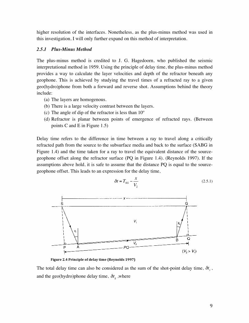
points C and E in Figure 1.5) Delay time refers to the difference in time between a ray to travel along a critically refracted path from the source to the subsurface media and back to the surface (SABG in Figure 1.4) and the time taken for a ray to travel the equivalent distance of the source-geophone offset along the refractor surface (PQ in Figure 1.4). (Reynolds 1997). If the assumptions above hold, it is safe to assume that the distance PQ is equal to the source-geophone offset. This leads to an expression for the delay time,

(2.5.1)

The total delay time can also be considered as the sum of the shot-point delay time, , and the geo(hydro)phone delay time, ,where

δt = TSG −xV2

δtsδtg

Figure  2.4  Principle  of  delay  time  (Reynolds  1997)  

  10  

(2.5.2)

(2.5.3)

As a result, the time taken by a ray following the critically refracted path can be expressed in terms of delay times, i.e.

(2.5.4)

Figure 2-5 Raypath geoetery from forward and reverse shots over irregular topography modified from (Reynolds 1997)

This is a useful approach to analyze the travel times of reverse and forwards shots to a given geo(hydro)phone as in Figure 1.5. Here, we are effectively concerned with three travel times:

(1) the time for a ray to travel from source 1 to source 2

(2.5.5)

(2) the time for a ray to travel from source 1 to geo(hydro)phone, D

(2.5.6)

(3) the time for a ray to travel from source 2 to geo(hydro)phone, D

(2.5.7)

Through the Hagedoorn plus term, T+, the sum of the travel times from shot to the geo(hydro)phone minus the overall travel time, it is possible to determine the delay time at D, and ultimately the depth to the refractor at D.

(2.5.8)

(2.5.9)

(2.5.10)

δts =SAV1

−PAV2

δtg =BGV1

−BQV2

TSG =xV2+δts +δtg

TS1S2 =LV2+δS1 +δS2

TS1D =xV2+δS1 +δSD

TS2D =(L − x)V2

+δS2 +δSD

T + = TS1D +TS2D −TS1S2 = 2δD

2δD =2zcosicV1

z = T +V12cosic

=T +V1V2

2(V22 −V1

2 )1/2

A

B

C E

G

F

  11  

The Hagedoorn minus term, T-, the difference in travel times taken by rays from each shot point to geo(hydro)phone D, can be used to determine the velocity of the refractor.

(2.5.11)

(2.5.12)

Plotting T- values against the offset distance x, will produce a curve with slope of 2/V2. The velocity of the upper layer, V1, can be obtained from the travel-time graph. Computing a plus and minus term for all detectors will provide a local refractor at each position.

3 Rayfract Refraction Tomography

3.1 Introduction Seismic refraction tomography allows for the imaging of subsurface velocity from seismic waves. It presents an alternative analytical method, and is particularly useful for deriving velocity structures of complex environments. Traditional analytical methods, like the ones mentioned in the previous chapter, are not adept at dealing with strong lateral changes in velocity, steep dips, or discontinuous refractors. Conventional analytical methods define layers by their interface, where each layer is assumed to have constant velocity and layers increase their velocity with depth (Sheehan et al. 2005). With refraction tomography, it is possible to resolve continuous velocity gradients and lateral velocity changes, and hence provide more realistic results in areas with extreme topography, strong lateral velocity variation or to analyze near-surface structures where there is no prior knowledge of the subsurface (Azwin et al. 2013). This study used Rayfract (version 3.23) to perform the tomographic imaging of the Äspö site. The tomographic model in Rayfract is based on Wavepath Eikonal Traveltime inversion (explained in section 3.3). A starting model is generated using Smooth inversion and the Delta-t-V method, which is refined to a 2D WET tomographic model. Rayfract can also estimate refractors using conventional methods, such as the plus-minus method. This section will give a brief background of the methods and procedure used in Rayfract to obtain the subsurface velocity model. For detailed information on the methods and algorithms used by Rayfract, and all its applications, I recommend visiting rayfract.com, where several references can be found.

T − = TS1D −TS2D

T − =2x − LV2

+δtS1 −δtS2

  12  

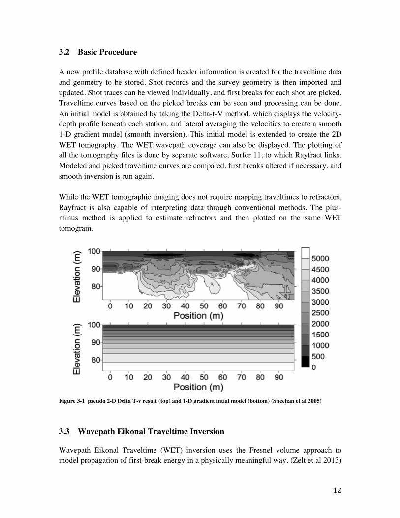
3.2 Basic Procedure A new profile database with defined header information is created for the traveltime data and geometry to be stored. Shot records and the survey geometry is then imported and updated. Shot traces can be viewed individually, and first breaks for each shot are picked. Traveltime curves based on the picked breaks can be seen and processing can be done. An initial model is obtained by taking the Delta-t-V method, which displays the velocity-depth profile beneath each station, and lateral averaging the velocities to create a smooth 1-D gradient model (smooth inversion). This initial model is extended to create the 2D WET tomography. The WET wavepath coverage can also be displayed. The plotting of all the tomography files is done by separate software, Surfer 11, to which Rayfract links. Modeled and picked traveltime curves are compared, first breaks altered if necessary, and smooth inversion is run again. While the WET tomographic imaging does not require mapping traveltimes to refractors, Rayfract is also capable of interpreting data through conventional methods. The plus-minus method is applied to estimate refractors and then plotted on the same WET tomogram.

Figure 3-1 pseudo 2-D Delta T-v result (top) and 1-D gradient intial model (bottom) (Sheehan et al 2005)

3.3 Wavepath Eikonal Traveltime Inversion Wavepath Eikonal Traveltime (WET) inversion uses the Fresnel volume approach to model propagation of first-break energy in a physically meaningful way. (Zelt et al 2013)

  13  

This means that instead of using rays to represent wave propagation, as is the case in conventional methods, WET applies wavepaths (Fresnel volumes or ‘fat rays’) to represent propagation. A Fresnel volume is defined by a set of waveforms that arrive within a half period of the fastest waveform (Sheehan et al 2005). Consequently ray paths are treated as beams with a finite length, thereby allowing the frequency of the wave to be introduced to the analysis (Watanabe et al. 1999). This avoids the assumption used in ray-path methods that the frequency of the source is infinite and, by extension, the wavelength is zero. As a result, the WET inversion model is able to take into account diffraction and scattering in the vicinity of the ray, which would have been missed using ray-path methods. This allows low-velocity zones and faults to be imaged with higher contrast. (Rayfract ® Help 2015)

Rayfract generates a 2D WET tomographic model by refining an initial 1D gradient model. This initial model is obtained using the Delta-t-V method followed by Smooth Inversion. The Delta-t-V method considers the offset distance, travel time, and apparent velocity, to create a pseudo 2-D Delta-t-V result of the individual velocity-depth profile under each station (see top image Figure 3.1). This helps detect small features and velocity inversions; however it does not remove artefacts, unrealistic imaged velocity variations. A smooth 1D gradient model is generated directly from the traveltime data by averaging the lateral velocities presented by the Delta-t-V method (see bottom image Figure 3.1). This allows the artefacts to be removed from the interpretation early on. (Rayfract ® Help 2015). Applying the smooth inversion process on Rayfract, to create the initial model, will then automatically begin also the 2D WET inversion. Along with

the tomographic image, Rayfract also generates a wavepath coverage plot after WET processing is complete. (Figure 3.2) This figure illustrates the paths of the seismic waves, showing concentration of waves along the model. The ray coverage is an important tool to analyze how well resolved the different structures in the WET tomogram are.

Figure  3.2  (a)  example  WET  tomogram  (b)  corresponding  coverage  plot  (Rayfract  ®  Help  2015)  

  14  

4 Study Area – Äspö Hard Rock Laboratory 4.1 Background The Äspö Hard Rock Laboratory (HRL) is an underground facility located on the Baltic east coast of Sweden, approximately 30 km north of Oskarshamn (see Figure 4-1). It was launched by the Swedish Nuclear Fuel and Waste Management Company (SKB) in 1986 as part of their work to design a deep geological repository for the final disposal of spent nuclear fuel. (Rhén et al. 1997) The underground part of the laboratory consists of a 3600 m long tunnel running from the Simpevarp peninsula, where the Oskarshamn nuclear power plant is located, to the southern part of the Äspö island where it spirals down to a depth of 460m. Above ground, SKB holds a ‘research village’ that contains offices, stores, an elevator down to the tunnel, and a ventilation building. The pre-investigation and construction phases of Äspö HRL were completed by 1995, during which the excavation of the tunnel and an extensive site characterization of the area took place. The first four years were dedicated to characterization of the rock both from ground surface and bore holes. (Stanfors et al. 1999) Several geoscientific investigation methods were performed to assess geological conditions and select the most suitable location for the HRL. From the collected information, models to outline the area were made. In 1995 the construction of the tunnel was completed. During the construction phase, geological studies continued and data could be collected from the laboratory tunnels. Monitored bore holes and bore holes drilled from the tunnel provided further information on the geological model and rock properties. These were compared with the pre-construction models, and as such offered a valuable evaluation of the pre-investigation methods used. (Rhén et al. 1997) While the preconstruction and construction phases focused on site characterization methods and demonstrated the suitability and efficacy of investigations at ground surface and in boreholes, the operation phase, starting from 1995, addresses itself to the study of safe disposal at the deep repository. Research is conducted to test the repository’s barriers’ abilities, understand the safety margins of the repository, and verify the technology used. (Stanfors et al. 1999) Äspö HRL is being used as a complete dress rehearsal for final disposal of spent fuel; practices from the depositing of canisters, to the plugging of tunnels and retrieval of deposited fuel are all being conducted with the objective to optimize the disposal method for simplification, cost efficiency and safety (SKB 2006).

  15  

The seismic refraction survey performed in this study covered the sea length between Hålö and Äspö, at a slight lateral offset from the tunnel plan. This chapter will continue by providing information on the geology concerning the study area, focusing on its lithology and structural model. The purpose is to gain a good understanding of the area to provide a basis and reference point for the results from the field investigation.

 Figure  4-­‐1 Location of the Äspö HRL; black line illustrates the tunnel profile(Stanfors et al. 1999)  

4.2 Geological Setting The bedrock found in the Äspö area falls in the Småland-Värmland belt, which forms part of the Trans-Scandinavian Igneous Belt (TIB). The TIB extends from southeastern Sweden, where the Småland-Värmland intrusions form, towards the north and northwest, into Norway. The rocks belonging to the TIB are primarily granitoids and volcanic rocks emplaced during repeated cycles of magmatism between 1.85 and 1.65 Ga (Larson and Berglund 1992). The Småland-Värmland belt is made up primarily of Småland granitoid, ranging from granite to quartz monzodiorite, (Gaal & Gorbatschev 1987). In the Äspo area they are dated to 18 Ma (Kornfält et al. 1997). Due to a continuous magma-mingling and magma-mixing process, mafic enclaves and dikes formed and resulted in an inhomogenous rock mass (Wikberg et al. 1991).

  16  

4.3 Lithological and Structural Model The models presented in this section are based on the geological investigation of the Äspö region completed during the pre-investigation and construction phases of Äspö HRL. One of the key issues decided for the site characterization was the geological-structural model, which describes the lithology and discontinuities of the rock types. (Rhén et al. 1997). This information was gathered by a collection of boreholes and ground surface investigations.

4.3.1 Lithology The bedrock of the Äspö region is made up of four main rock types: Äspö diorites, Ävrö granite, greenstone, and fine-grained granite (summary of characteristics Table 4-1). The distribution is mainly from Ävrö granite, which occurs principally on the Ävrö island and southern part of Äspö to Äspö diorite, which occurs mainly on the northern part of Äspö. (Stanfors et al. 1999). The dominant rock types, Äspö diorites and Ävrö granite, are both Småland granitoids. Initially they were distinguished by their color and content of megacrysts, but upon later investigations distinctions were made by their density. With the calculated content of magnetite subtracted, the densities were given by: granite 2.641-2.7 kg/dm3 and diorite 2.701-2.8 kg/dm3. (Berglund et al. 2003)

The greenstones are composed mainly of mafic rock types and occur as minor inclusions within the granitoids and dioritoids. Fine-grained granites appear as dikes or irregular veins throughout all the rock mass, trending mainly NE. They are most common in the Äspö diorite. (Rhén et al. 1997) The irregular distribution of greenstone and fine-grained granite makes it difficult to describe the exact position and extent of minor rock units.

Material Properties

Äspö Diorite Grey and reddish-grey color medium grained granodiorite, quartz monzonite, and quartz diorite

Ävrö Granite

Brighter, Reddish-grey Medium grained, finely-medium grained Granites and granodiorites

Greenstone Very dark, greenish or greyish-black Fine-grained and medium to coarse-grained Diorites to gabbros

Fine-grained granites Reddish grey to red Fine-grained True granite

Table 4-1 Summary of main rock types found in Äspö region and their properties

  17  

4.3.2 Fracture Zones The Äspö tunnel area is intersected by a number of fracture zones. The pre-investigation phase of Äspö HRL divided discontinuities into major fracture zones (width>5m) and minor fracture zones (width<5m). Most fractures are oriented northwest–southeast, although the majority of the shear zones are oriented southwest–northeast. (Berglund et al. 2003) The most important fracture zones to the tunnel area are pictured in figures 4-2 and 4-3 and are briefly described below, from north to south. This description of the bedrock structure is based on earlier technical reports published by SKB / (Stanfors et al. 1997); (Stanfors et al. 1999);(Rhén et al. 1997)

Fracture Zone

Position along main tunnel

(center of zone)

Strike

Dip

Width (m)

NE2 1602 m N15-36°E 70-80°S 1-6

EW3 1414 m N80°E 75-80° 14

NE1 1284 m N50-55°E 70-75°N 61

NE3 992 m N60°E 75°N 49

NE4 828 m N50°E 60°S 41

EW7 787 m N75°E 75°S 10 Table 4-2: Summary of major fracture zones. Modified from(Stanfors et al. 1997)

EW3: Found to be approximately 12m wide in the tunnel, and consists of 2-3 m wide central section of fault crush material related to contact between Äspö dirote and fine-grained diorite (Stanfors et al. 1999).

NE1: Compromises of three branches related to a rather complex rock mass with Äspö diorote, fine-grained granite, and greenstone. The two southernmost branches can be described as highly fractured and hydraulically conductive. The northern branch is the most intensely fractured and produces significant inflow.

NE3: The fracture zone dips steeply towards NNW, however it’s constituent fractures are steep and strike EW and NS. Associated with several dikes of fine-grained granite and some mylonites (Wikberg et al. 1991).

NE4: Consists of two more or less continuous branches, containing Ävrö granite with inclusions of mylonite and greenstone.

EW7: When encountered in tunnel, consists of one set of fractures trending NNE, which is the most hydraulically conductive here, and one set of fractures trending WNW.

  18  

In addition to the major fracture zones, a number of minor fracture zones exist in the Äspö tunnel area that trend WNW-NNW (Rhén et al. 1997). The relevance of the minor fracture zones, which range from 10cm to a few meters wide, to this investigation is small becauset he refraction spacing used was 5 meters. Anything smaller than 5 meters will be difficult to resolve.

4.3.3 Quaternary Deposits Quaternary deposits refer to the loose deposits overlying the bedrock, which in the Äspö region are scarce. Given most of the investigation conducted for the Äspö HRL was geared towards construction in deep rock setting, extensive data concerning the sediments is limited, particularly on the Äspö side. Most of the investigations completed regarding the quaternary deposits were to study their effects on groundwater flow. Soil cover around Äspö is generally thin with a thickness between 0 and 5 meters, consisting mainly of clay, sand and gravel (Vidstrand 2003) The rock outcrop is extensive throughout both the Äspö island and Simpevarp peninsula, however in low areas the soil cover may reach 5 to 10 meters in depth (Curtis et al. 2003).

Figure  4-­‐2  Fracture  zones  in  Äspö  HRL  model  in  the  pattern  of  regional  structures  (Stanfors  et  al.  1999)

  19  

5 Field Investigation of Äspö The field investigation at Äspö was performed on April 20-24, 2015, between the northern part of Hålö and the southern part of Äspo (see Figure 5-1). Measurements were collected just west of the tunnel line, approximately 10 meters off the small island between Äspö and Hålö. Seismic refraction surveying was done primarily on the sea bed, with a couple of sensors off the water, on a 450 m line. Simultaneous to the seismic refraction survey, DCIP and resistivity measurements were carried out both on the sea bed and on land; these results can be found in Erik Fennvik’s work, “Resistivitet- och IP-mätningar vid Äspö Hard Rock Laboratory”. This chapter will describe the seismic refraction study that took place and display the results in a 2D WET tomographic velocity model.

Figure  4-­‐3  Structural  model  of  vertical  section  along  the  line  of  the  tunnel  ramp  (Stanfors  et  al.  1999).

  20  

Figure 5-1 Location of seismic refraction survey at Äspo HRL. Measurement profile is given by the red line

5.1 Data Acquisition A seismic refraction profile was conducted along the line shown in Figure 5-1 using two hydrophone streamers. Both hydrophone streamers were towed by boat and laid out manually along the seabed. The hydrophone spread consisted of 91 hydrophones at 5 meter spacing. Two portable seismographs, placed at the small island between Äspo and Hålö, recorded the arrival times of the seismic waves at each receiver. The instruments used were (a) 48- channel ABEM Terraloc and (b) 48-channel Geometrics Stratavizor. This gave a total of 96 channels, 91 of which represented active unique hydrophone positions. Exact positions of the receivers were determined by a differential GNSS. The seabed was mapped using a multibeam echosounder. Seismic waves were generated using small explosives set off approximately 0.5 meters above the seabed. Shot intervals were 20 meters, however because of time constraints shots were not fired at all the planned stations. Figure 5-2 displays the hydrophone spread and positions of the shots; shots were not fired at stations 67, 71, and 79.

  21  

Figure 5-2 Coordinate position of receivers and shots along hydrophone streamer

The use of two different sets of equipment – ABEM Terraloc and Geometrics Stratavizor – entailed extra attention to ensure both instruments triggered at each shot. Channels 1-48, positioned on the south side of the profile line, were given by the Terraloc, and channels 44-91 were given by the Stratavizor. There was a 4 hydrophone (20m) overlap.

Figure 5-3: South-facing image of boat along the seismic profile. Buoys show where shots were fired and the island where the seismographs were located is seen on the left.

     

5.2 Data Processing All processing of the data was done using Rayfract refraction tomography software. Raw data from shot records were imported into a new profile database with header and geometry defined by coordinate positions of receivers and shots. Traveltime curves from each shot were considered individually to pick the first arrivals manually. Once first arrivals had been picked for each shot, smooth inversion was run to generate the 2D WET tomography image of the subsurface velocities. Traveltimes were mapped to refractors

6367200  

6367250  

6367300  

6367350  

6367400  

6367450  

6367500  

6367550  

6367600  

6367650  

6367700  

6367750  

159700   159710   159720   159730   159740   159750   159760   159770   159780  

Y  Co

ordina

te  

X  Coordinate  

Receivers  

Shots  Fired  

  22  

and two-layer based Plus-Minus refraction interpretation was applied. The velocity-distance curve was compiled to the velocity model.

(a) Shot ch. 31, Channel view 1-48 (b) Shot ch.87, Channel view 44-91

(c) Figure 5-4 Processing of data on Rayfract. (a) and (b) illustrate picked first breaks at two different receiver

stations along the profile. (c) travel-time curves of entire profile, squares indicate were traces were mapped to refractors

The nature and quality of the data differed between the two ends of the profile (see Figure 5-4), and by extension between the instruments used. Though they displayed little noise, Channels 1 through 48 generally showed faint data, making picking of first breaks challenging. Moreover, arrivals of the refractors were not readily seen on the traveltime curves. Channels 44-91 provided more workable data as traces could be mapped to refractors. At channels where noise was evident, i.e. 46, 57, 70, and 79, arrivals could not be picked.

  23  

This contrast between the north and south side of the survey is clearly displayed in the travel-time curve in Figure 5-3 (c), where the shift happens between stations 45 and 50. Due to the complex and varied nature of the data, conventional methods of interpretation would have been immensely time consuming to complete and probably inaccurate. Owing to the imperfect data gathered on the south side of the profile, there was not enough coverage on the shots between stations 1 and 48 to apply an accurate plus-minus interpretation of this section. Rayfract issued low data coverage warnings and attempted to extrapolate extra data to compensate for the poor coverage, however it was not successful. The plus-minus velocity section therefore was only applied to the northern side of the profile, from 250 to 450 m along the x-axis.

5.3 Results The resulting tomographic velocity model of the Äspö-Hålö line is shown in Figure 5-4, along with a plot of the wave coverage. Four subsurface layers defined by their seismic velocities can be observed, illustrated on the model by the change in colors.

Layer Color on Model Velocity Range (ms-1)

Interpreted Material

1 Blue 1600-2600 Sand and Clay

2 Green 2600-4200 Solidifed/Compacted soil or

moderately fissured/weathered to

highly weathered rock, granite

3 Yellow 4200-4800 Slightly fissured/weathered rock,

granite

4 Red 4800-6200 Fresh rock, granite Table 5-1 Summary of material of subsurface layers

With a P-wave velocity between 1600 and 2600 ms-1, the top layer is considered to consist of unconsolidated materials such as sand and clay. Following this first layer starts the transition into the bedrock, which is depicted by the hatched line in Figure 5-5 (a). Layer 2, with velocities between 2600 and 4200 ms-1 can be classified as compacted soil due to the high pressure of the overburden and water, or highly weathered granite. The

  24  

bedrock, known to be made up of Småland granitoid, is predicted to progress from a highly weathered state to sound rock. Depth to the bedrock varies along the profile, which is marked by undulating layers and depressions. On the south side of the profile the depth to bedrock reaches up to 78m and on the north side the depth to the bedrock can reach up to 16m. The first 250m of the profile comprises of a major depression, reaching 80 m below the seabed. This deep depression coincides with the location of fracture zones NE3 and NE4, which as described in the previous chapter, strike NE and dip 75°N and 60°S respectively. Data coverage above the depression is very poor. The black segment between 50 and 150 m in Figure 5-5 (b) indicates no ray coverage was given here. Ray coverage between 250 and 450 m along the x-axis is good. The plus-minus velocity section is mapped in Figure 5-4 (a) by crosses. It generally corresponds with the velocity tomogram, though the bedrock is found deeper, given to dip 16 to 19 meters below the surface. The inability to map the entire profile through plus-minus methods reduces the reliability of this interpretation however, so more confidence should be given to the tomogram results.

5.4 Discussion The profile structure of the Äspö-Hålö line as shown by the resulted velocity model is uncharacteristically heterogeneous. The strongest shift occurs at 250m and is marked by the major depression on the south side. As the approximate mid point of the profile, this shift coincides with the change in hydrophone streamers and seismographs. Difference in equipment, however, was ruled out as a reason for the contrast upon referral to the DCIP results, which verified the depression on the southern end. Given the lack of coverage inside the depression, it is impossible to know for sure what this area is composed of. However, this anomalous feature of the profile can be explained by the known locations of fracture zones NE3 and NE4, whose opposite dips could indicate the presence of a horst-graben structure. Horsts and graben are blocks bounded by faults that have been raised (horst) or lowered (graben) relative to their surrounding. They are marked by sharp slips in the rock where the faults occur. This sharp variation could not have been picked up because of smoothing constraints of the model.

  25  

(a)

(b)  

Figure 5-5 a) Rayfract WET tomography velocity model of profile. Hatched line indicates start of bed rock, crosses indicate plus-minus interpretation (b) Ray coverage of the WET tomography model  

At this stage, with the limitation of data on the south side of the profile, only hypotheses can be made to explain the anomaly of the profile. However, ray coverage is a good

  26  

indication of the reliability of the velocity model and provides a means to critically analyze the results. Looking at the ray coverage in Figure 5-2 (b), it is clear the seismographs did not detect any rays travelling through the depression. This could be because rays travelling below an irregular section caused by the horst-graben, at a higher velocity layer, would arrive much earlier than those following the complex nature of sudden changes in interface depth. The dips on the northern side of the profile, between 250 and 450 m, could be due to either depression in the bedrock, or a large low velocity zone consisting of highly weathered or altered rocks. Ray coverage along this side of the profile is good, indicating that results can be taken with more confidence. It is important to note that the 2D WET tomogram images smooth gradients of velocity, and consequently shows averages along the profile. As such it is difficult for thicknesses of layers to be discretely evaluated. Nonetheless it was possible to resolve four layers gradually increasing in velocity. Composition of the layers was interpreted as clay and sand on the top layer, followed by solidified soil and weathered granite, with sound rock at the bottom. This interpretation was based on the geological overview of Äspö presented in the previous chapter. There are limitations in the interpretation that result from different sources of uncertainties both in the scope of field data and uncertainties in the software itself may present limitations to the interpretation of the results. . Some sources of uncertainties could include:

-­‐ Large differences between modeled and picked travel times -­‐ Seismic noise -­‐ Incorrect first arrival picking -­‐ Errors in the instruments -­‐ Geographical or geometrical errors (i.e. errors in receiver and shot coordinates or

bathymetry.) Errors due to instruments and geographical settings are unlikely. In this case, the most probable source of uncertainty on the south side is due to the low coverage, and on the north side due to seismic noise apparent in certain channels. The tomographic model generated by Rayfract is only an estimation of the subsurface conditions. Follow up investigations are necessary to validate the outcome model, justify the predicted presence of a horst-graben structure, and determine the nature of the undulating rock mass on the northern side. Borehole drillings at 150m, 300m and 400m along the x-axis would provide information at the necessary detailed scale to verify the interpretation.

  27  

6 Conclusion Three important characteristics of the Äspö-Hålö profile, located along the Äspö Hard Rock Laboratory access tunnel, could be determined by seismic refraction methods. These were:

1. Depth to the bedrock along the profile 2. Layer interface structure and its composition 3. Geological features and weak zones in the bedrock

The resulting velocity model imaged four layers along the Äspö-Hålö profile, progressing from a top layer of sand and clay to fresh granite at the bedrock. The intermediate layers were interpreted as solidified soil and granite at varying degrees of weathering. Depth to bedrock varies along the profile due to an undulating trend of the rock mass, however it reaches approximately 78m on the south side and 16m on the north side. The Äspö-Hålö profile showed a unique result marked by the strong contrast between its northern and southern end. The interpretation of the model concludes that the obstruction of ray paths on the southern side of the profile is caused by a horst-graben structure bounded by the fracture zones NE3 and NE4. Weak zones in the bedrock are found on the northern end of the profile, at 300 and 400 m along the x-axis, depicted by the low-velocity area. This could also be interpreted as a depression in the bedrock. Rayfract proved to be an appropriate tool for interpretation given the velocity and depth variations of the layer interfaces. Conventional methods of interpretation would have been ineffectual due to the nature of the data and complex characteristics of the bedrock, particularly amongst channels 1-48. Moreover, wave coverage plots accompanying Rayfract’s model output allowed for a possibility of quality control not available in conventional methods. Where the tomography inversion falls short, however, is in its velocity gradients, which make detection of sharp layer interfaces very difficult. In a case like the Äspö-Hålö line, where circumstances of the geological features greatly impacted the data coverage, it becomes necessary to do follow up investigations. Points of interest could be determined through the seismic refraction survey, namely at 150 m, 300m and 400m along the x-axis. These are locations that should be further studied through different investigative methods, such as borings. Information gathered by this seismic refraction survey is particularly useful for problems in civil engineering, where a good understanding of ground conditions is imperative. Depth to bedrock and knowledge of bedrock quality and conditions is fundamental for

  28  

any foundation study. The advantages of seismic refraction over traditional geotechnical methods, which can provide similar information, lies in its ability to model continuous areas. While traditional geotechnical methods of site investigation, such as core drilling, deliver more precise information at specific locations, the seismic refraction model averages results over a large area. As such value is placed on the ability to assess conditions on a grand scale. The Äspö-Hålö profile is a good example of a site where information over a continuous line is particularly beneficiary. The contrasting conditions of the southern and northern side of the profile, as well as the complex and varied bedrock line, make up a complicated geological environment that could not have been appreciated through investigation at a discrete point. However it must also be noted that as a method that averages the velocities across the profile, detailed conclusions cannot be drawn based on seismic refraction alone. As such, it can be concluded that an effective site investigation that presents a holistic view of ground conditions requires an integration of different methods. As demonstrated in this study of Äspö, seismic refraction is suited to find depths to bedrock, layer interfaces, and critical areas in the subsurface. While on the one hand it provides valuable insight on locations for test and core drilling, on the other, it depends on background knowledge on the lithological and structural model of the investigated area for fruitful interpretation. Accordingly, this geophysical method acts like a good bridge in an integrated site investigation.

  29  

7 References

Azwin, I.N., Saad, R. & Nordiana, M., 2013. Applying the Seismic Refraction Tomography for Site Characterization. , 5, pp.227–231.

Berglund, J. et al., 2003. Äspö Hard Rock Laboratory. Update of the geological model. SKB (Swedish Nuclear Fuel and Waste Management Company) IPR-03-34.

Curtis, P., Elfström, M. & Stanfors, R., 2003. Oskarshamn site investigation. Compilation of structural geological data covering the Simpevarp peninsula, Ävrö and Hålö. SKB (Swedish Nuclear Fuel and Waste Management Company) P-03-07. Available at: http://skb.se/upload/publications/pdf/P-08-101Webb.pdf.

Gaal, G. & Gorbatschev, R., 1987. An Outline of the Precambrian Evolution of the Baltic Shield. Precambrian Research, 35, pp.15–52.

Kornfält, K., Persson, P. & Wikman, H., 1997. Granitoids from the Äspö area, southeastern Sweden ‐ geochemical and geochronological data. GFF, 119(2), pp.109–114.

Rhén, I. et al., 1997. Äspö HRL-Geoscientific evaluation 1997/2 Results from pre-investigations and detailed site characterization. SKB (Swedish Nuclear Fuel and Waste Management Company) TR-97-03.

Sheehan, J.R., Doll, W.E. & Mandell, W. a., 2005. An Evaluation of Methods and Available Software for Seismic Refraction Tomography Analysis. Journal of Environmental & Engineering Geophysics, 10(1), pp.21–34.

SKB, 2006. The Äspö hard rock laboratory. Available at: http://www.skb.se/upload/publications/pdf/Aspo_Laboratory.pdf.

Stanfors, R. et al., 1999. Overview of geological and hydrogeological conditions of the Aspo hard rock laboratory site. Applied Geochemistry, 14(7), pp.819–834.

Stanfors, R., Olsson, P. & Stille, H., 1997. ÄSPÖ HRL – Geoscientific evaluation 1997/4. Results from pre-investigations and detailed site characterization. Comparison of predictions and observations. Hydrogeology, groundwater chemistry and transport of solutes. , (May).

Vidstrand, P., 2003. Äspö Hard Rock Laboratory. Update of the hydrogeological model 2002. SKB (Swedish Nuclear Fuel and Waste Management Company) IPR-03-35.

Watanabe, T., Matsuoka, T. & Ashidi, Y., 1999. Seismic traveltime tomography using Fresnel volume approach. Kyoto University, Japan.

  30  

Wikberg, P. et al., 1991. Äspö Hard Rock Laboratory. Evaluation and conceptual modelling based on the pre-investigations 1986-1990. SKB (Swedish Nuclear Fuel and Waste Management Company) Techincal Report 91-22, (June).

Zelt, C et al., 2013. Blind Test of Methods for Obtaining 2-D Near-Surface Seismic Velocity Models from First-Arrival Traveltimes. Journal of Environmental and Engineering Geophysics, vol. 18. no. 3, pp. 183–194.