Äspö hard rock laboratory - skb · tbt (temperature buffer test) is a joint project between...

Svensk Kärnbränslehantering ABSwedish Nuclear Fueland Waste Management Co

Box 250, SE-101 24 StockholmPhone +46 8 459 84 00

InternationalProgress Report

IPR-08-09

Äspö Hard Rock Laboratory

Temperature Buffert Test

Evaluation modellingTBT_3 Mock-up test

Edited by

Mattias Åkesson

Clay Technology AB

May 2008

Report no. No.

IPR-08-09 F12KAuthor Date

Mattias Åkesson May 2008Checked by Date

Bertrand Vignal July 2008Approved Date

Anders Sjöland 2008-11-10

Keywords: Buffer, Bentonite, THM, Mock-up, Test, Temperature, Hydration, Stress,Strain

This report concerns a study which was conducted for SKB. The conclusionsand viewpoints presented in the report are those of the author(s) and do notnecessarily coincide with those of the client.

Äspö Hard Rock Laboratory

Temperature Buffert Test

Evaluation modellingTBT_3 Mock-up test

Edited by

Mattias Åkesson

Clay Technology AB

May 2008

3

Résumé

TBT (Test de Barrière ouvragée en Température) est un projet mené dans le Hard Rock Laboratory d’Äspö en Suède par SKB et l'ANDRA, soutenu par ENRESA et DBE, qui vise à comprendre et modéliser le comportement thermo-hydro-mécanique de barrières ouvragées à base d’argile gonflante soumises à des températures élevées (> 100°C) pendant le processus de leur hydratation.

Depuis le début du projet, différentes tâches de modélisation ont été continûment développées. Les calculs de dimensionnement et les modélisations prédictives de la désaturation initiale du test in situ ont été antérieurement rapportés.

Le présent rapport couvre les prévisions et les évaluations relatives au test TBT_3 réalisé sur maquette en 2006 par le CEA à Saclay (France). Le test portait sur les processus de désaturation observés sur le test TBT in situ autour de la sonde chauffante inférieure.

Le test sur maquette TBT_3 a été modélisé en utilisant le Code_Bright pour des analyses TH et THM qui ont produit d’importants résultats. En régime permanent, la pression de vapeur d’eau présente une distribution assez homogène, ce qui indique que le gradient de pression de vapeur domine le transport de l’eau en non saturé. Par ailleurs, une évaluation des propriétés de rétention montre que le matériau bentonite, même non saturé, pourrait être en équilibre avec la vapeur saturée. Il convient alors, pour modéliser précisément la redistribution de l’eau, d’ajuster la courbe de rétention. Il a aussi été établi que le comportement mécanique observé dans TBT_3 peut être bien reproduit en utilisant le modèle développé à Barcelone et basé sur une double structure BExM. Ces différents résultats pourraient être utilisés dans des travaux de modélisation du test TBT in situ.

5

Abstract

TBT (Temperature Buffer Test) is a joint project between SKB/ANDRA, supported by ENRESA and DBE, carried out in granitic rock at Äspö Hard Rock Laboratory, Sweden. The test aims at understanding and modeling the thermo-hydro-mechanical behavior of buffers made of swelling clay exposed to high temperatures (over 100°C) during the water saturation process.

Since the beginning of the project, different modeling tasks have continuously been carried out. Previously, scoping design calculations, predictive modeling of initial field test desaturation and evaluation modeling of field test issues have been reported.

The present report covers predictions as well as evaluations of a mock-up test (TBT_3), carried out by CAE in Saclay (France), addressing the desaturation process observed in the field test around the lower heater. This task was carried out during 2006.

The TBT_3 Mock-up test was modeled using Code_Bright for both TH and THM analyses. This task revealed a number of important results. At steady-state, the vapor pressure exhibited a quite homogenous distribution. This indicates that the vapor pressure is the dominating potential for moisture transport at unsaturated conditions. An evaluation of the retention properties revealed that the bentonite material can apparently be in equilibrium with saturated vapor, even though the material was not water saturated. To model the moisture redistribution with precision, the retention curve had to be modified accordingly. It was also found that the mechanical behavior in test like TBT_3 can be well reproduced with the BExM constitutive laws, based on a double structure model. These results should be addressed in attempts to model the field test.

7

Sammanfattning

TBT (Temperature Buffer Test) är ett gemensamt SKB/ANDRA projekt, med deltagande av ENRESA och DBE, vilket utförs i granitiskt berg vid Äspö HRL i Sverige. Syftet är att öka förståelsen för, och att modellera, de termiska, hydrauliska och mekaniska processerna i en buffert av svällande lera som utsätts för höga temperaturer (över 100°C) under bevätningsfasen.

Olika modelleringsinsatser har utförts kontinuerligt sedan projektet startades. Tidigare har inledande beräkningar (scoping design) samt prediktiva modelleringar av den initiella uttorkningen av fältförsöket rapporterats.

Den föreliggande rapporten omfattar prediktioner och utvärderingar av ett mock-up försök (TBT_3), utfört av CEA i Saclay (Frankrike), vilket efterliknade den uttorkningsprocess som har observerats runt den nedre värmaren i fältförsöket. Insatsen utfördes under 2006.

Mock-up försöket TBT_3 modellerades med Code_Bright för såväl TH som THM analyser. Denna insats avslöjade ett antal viktiga resultat. Vid steady-state uppvisade ångtrycken en tämligen homogen fördelning. Detta indikerar att ångtrycket är den dominerande potentialen för fukttransport vid omättade förhållanden. En utvärdering av retentionsegenskaperna visade att bentoniten uppenbarligen kan vara i jämvikt med mättad ånga, även om bentoniten inte är vattenmättad. För att kunna modellera fuktomfördelningen med noggrannhet var det följaktligen nödvändigt att modifiera den använda retentionskurvan. Det visade sig också att det mekaniska beteendet i tester som TBT_3 kan reproduceras väl med de konstitutiva sambanden i BExM, vilka baseras på en dubbelstrukturmodell. Dessa resultat bör beaktas i modelleringsinsatser av fältförsöket.

9

Contents

1 Introduction 11

2 Experimental work 13 2.1 General 13 2.2 Material and methods 13 2.3 Results 14

3 Modeling work 19 3.1 General 19 3.2 Predictions 19 3.3 Evaluations 21

4 Concluding remarks 25

5 References 27

Appendix I: Modeling program 29

Appendix II: Predictive modeling UPC 39

Appendix III: Predictive modeling ClayTech 61

Appendix IV: Evaluation modeling UPC 83

Appendix V: Evaluation modeling ClayTech 121

11

1 Introduction

TBT (Temperature Buffer Test) is a joint project between SKB/ANDRA, supported by ENRESA and DBE, carried out in granitic rock at Äspö Hard Rock Laboratory, Sweden. The test aims at understanding and modeling the thermo-hydro-mechanical behavior of buffers made of swelling clay exposed to high temperatures (over 100°C) during the water saturation process.

Within the framework of the TBT modeling task force, it has been decided to consider particularly the thermo-hydraulic conditions around the lower heater in the TBT test. In the field experiment, there was a significant and fast dehydration in an approximately 0.15 m wide annular zone around the heater /Goudarzi et al., 2005/. The temperature increased to just below 130 °C during the first 20 days. The temperature gradients were almost 4.5 °C/cm in the region where desaturation appeared to have taken place. The pattern of desaturation and its time-scale has raised the question whether the thermal gradient alone or the combination of high temperatures and high thermal gradients is responsible for the process. However, it is not possible to infer any such information directly from field test. The high gradient close to the heater was partly an effect of the drying, and not the clear-cut cause of it. At some distance from the heater, there was no drying. This may well be an effect of moisture moving in from the regions close to the heater, rather than an indication of insufficient thermal gradients.

The approach decided by ANDRA and the TBT modeling teams was two-fold, with a lab-scale mock-up test combined with a predictive modeling task, and addressed the phenomenon of desaturation and the relative importance of temperature gradients and temperature levels.

A mock-up, TBT_2, test was planned and designed at the CEA laboratory in Paris, France. The basic idea was to subject a confined sample of MX-80 bentonite material to thermal gradients similar to those around the lower heater in the TBT field experiment, and to monitor the development of temperature, relative humidity and stress during a well-defined sequence of thermal loading. All predictions and test results showed that moisture redistribution takes place as soon as there are thermal gradients. Results therefore do not support the notion of thermal threshold gradients. Models also showed that it is the temperatures at the hot and cold ends rather than the thermal gradient that determine the extent of moisture redistribution (i.e. the shape of the steady-state saturation profile), independent of the sample length.

During the course of the work with TBT_2 it was found that the experiment suffered from a thermal leakage. A new experiment with a new modeling task, TBT_3, was therefore defined. Measures were taken to avoid the thermal leakage in this experiment. The test was more instrumented than previously, while the applied thermal protocol was simpler.

This report describes the experimental as well as the modeling work

13

2 Experimental work

2.1 General The TBT_3 mock-up was performed by CEA in Saclay in France, and the work has been described in detail by Gatabin and Guillot (2006). A brief description of the experimental work and the results are given in the following paragraphs.

2.2 Material and methods A cylindrical rigid cell was equipped with heaters for temperature control at the two circular faces of a contained bentonite specimen. The cell was densely instrumented with sensors for measurements of temperature, relative humidity, pore pressure, radial stress and the axial stress through the mobile piston.

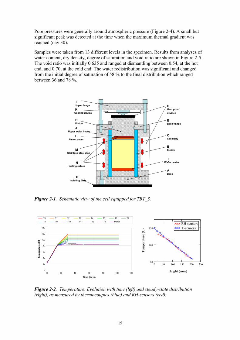
The design of the cell is illustrated in Figure 2-1. The base, the cell body, the back and upper flange, as well as the piston were made of stainless steel. The sleeve on the inside of the cell body was made of pure PTFE and had a thickness of 17 mm. The joints between the base and the cell body and between the back flange and the piston were sealed with O-rings.

The wafer heaters used for temperature control at the upper and lower faces of the specimen consisted of hollow copper plates in which heating cables were wound. Each heater was fitted by two temperature probes embedded in the coil, one in the centre and the other at 60 -70 mm from the centre. The central probes were used for temperature regulation. Three heating cables were rolled up around the cell body at ¼, ½ and ¾ height of the specimen. The temperature at each height was measured by a thermocouple fixed in a hole bored in the cell body. Each heater and cable was supplied by a power device controlled by a process regulator. All process regulators were set independently.

The specimen was made of MX-80 bentonite powder, which was conditioned in climate chamber in order to increase its water content to 13.3 %. A bentonite core was compacted isostatically to a dry density of 1.70 g/cm3. With a solid density of 2.78 g/cm3, this corresponds to a saturation degree of 58.6 %. The core was finally machined to a diameter of 202.5 mm and a height of 202 mm, thereby adjusted to match the total available volume in the PTFE containment sleeve.

The bentonite specimen was fitted with 14 temperature probes; 11 capacitive relative humidity (RH) sensors; and four pore-pressure sensors. Within the specimen, a cylindrical safety zone of 5 cm diameter was preserved without any sensor in such a way that it could be cored at the end of the test for analysis purpose. One relative-humidity sensor, HR10, acted as peripheral sensor, its sensitive part being close to the cylindrical envelope. All sensors were laid out perpendicularly to the vertical axis of the cell. Three total pressure sensors were installed in the cell body for monitoring of radial stresses. A list of sensors and their locations is shown in Table 2-1. A load cell was used for monitoring of the axial stress through the mobile piston.

14

The cell was thermally isolated with 50 mm thick rock-wool strips enveloping the cell body. The base was placed on a low-conductivity plate.

The defined thermal protocol was divided in three phases: (i) an initial homogenous thermal ramping during 15 days from room temperature at 22°C up to 84°C, (ii) a temperature increase at the hot face during 15 days up to 120°C, with cold face temperature constant at 84°C, and (iii) an equilibration phase with constant thermal gradient. The latter phase was allowed to continue for 72 days. In total, the experiment was run for 102 days. The target temperatures for the heating cables were set to correspond to a linear temperature distribution, i.e. for a temperature gap between 84 and 120°C, the target temperatures were 93, 102 and 111°C, respectively.

After switching off the heaters and removing the external layer of heat insulation, the specimen was allowed to cool for approximately 20 hours. The experiment was dismantled by removing the upper flange, the back flange, the piston and the stainless steel disc. Bentonite samples were finally recovered by vertical coring of a 50 mm diameter cylinder in the centre of the specimen. This core was sampled and analyzed for bulk density, through weighing in petroleum, and water content.

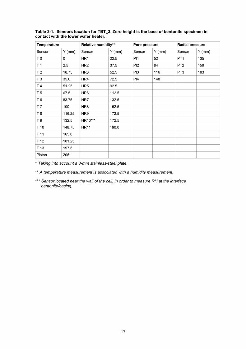
2.3 Results The original thermal protocol was followed in detail (Figure 2-2), and the registered temperatures show that the heating system worked as planned. The temperate at the cold end of the specimen (T13) was however slightly lower (up to 3˚C) than the hot end (T0) during the initial phase with prescribed homogenous temperature. The linear temperature distribution, specified by the target values of the heating cables, was also reflected by the thermocouple readings. Temperatures from thermocouples and RH-sensors were generally in agreement. Values from RH-sensors at the hot end were slightly lower than the corresponding values from the thermocouples. At the end of the measurements, the heaters were turned of so that the sample could cool. This condition was maintained for 20 hours, and during this period the temperatures dropped to 28 – 35 ºC.

The evolution and the distributions of relative humidity, at steady-state and after cooling, are shown in Figure 2-3. During the initial phase the RH-values increased generally from 60 % to values between 67 and 79 %. This separation of RH-levels was probably caused by the minor temperature difference noticed during the initial phase. A more significant separation was registered during the second phase when the thermal gradient was applied. At the end of the phase the values ranged from 60 to 96 %. The HR6 sensor failed during this phase. The separation continued during the final phase with RH-values at steady-state ranging from 40 to 100 %. It can be noted that the three uppermost sensors at the cold side (HR9 – HR11) showed 100 %. Sensor HR8 equilibrated at a slightly higher level of 104 %.

The build-up of stresses is shown in Figure 2-4. The radial sensor closest to the cold side (PT3) registered the highest stress, with a peak value of 6.5 MPa. The axial stress and the radial stress closest to the mid-section (PT1) equilibrated at 2 – 3 MPa. The PT2 sensor was located between PT1 and PT3, and it could therefore be expected that the stress level at this point would fall between 3 and 6 MPa. Instead, the stress was lower (< 1 MPa). This deviation was probably caused by a bad contact between the sensor membrane and the specimen.

15

Pore pressures were generally around atmospheric pressure (Figure 2-4). A small but significant peak was detected at the time when the maximum thermal gradient was reached (day 30).

Samples were taken from 13 different levels in the specimen. Results from analyses of water content, dry density, degree of saturation and void ratio are shown in Figure 2-5. The void ratio was initially 0.635 and ranged at dismantling between 0.54, at the hot end, and 0.70, at the cold end. The water redistribution was significant and changed from the initial degree of saturation of 58 % to the final distribution which ranged between 36 and 78 %.

GIsolating plate

ABase

IWafer heater

B Sleeve

CCell body

EBack flange

HHeat proofdevices

JUpper wafer heater

DPiston

KCooling device

FUpper flange

LPiston cover

MStainless steel disc

NHeating cables

Figure 2-1. Schematic view of the cell equipped for TBT_3.

0

20

40

60

80

100

120

140

0 20 40 60 80 100 120

Time (days)

Tem

pera

ture

(C9

T0 T1 T2 T3 T4 T5 T6 T7 T8 T9 T10 T11 T12 T13 Piston

0 50 100 150 200 25080

100

120

RH-sensorsT-sensors

Height (mm)

Tem

pera

ture

(C)

Figure 2-2. Temperature. Evolution with time (left) and steady-state distribution (right), as measured by thermocouples (blue) and RH-sensors (red).

16

0

20

40

60

80

100

120

0 20 40 60 80 100 120Time (days)

Rel

ativ

e hu

mid

ity (%

)

HR1 HR2 HR3 HR4 HR5 HR6

HR7 HR8 HR9 HR10 HR11

0 50 100 150 20020

40

60

80

100

120Steady-stateAfter cooling

Height (mm)

Rel

ativ

e hu

mid

ity (%

)

Figure 2-3. Relative humidity. Evolution with time (left); Final distributions (right): at steady-state (red) and after cooling (blue).

0

1

2

3

4

5

6

7

0 20 40 60 80 100 120

Time (days)

Stre

ss (M

Pa)

PT1 135 mm PT2 159 mm PT3 183 mm Axial

0

0,05

0,1

0,15

0 20 40 60 80 100 120

Time (days)

Por

e pr

essu

re (M

Pa)

Pl1 52 mm Pl2 84 mm Pl3 116 mm Pl4 148 mm

Figure 2-4. Build-up of stresses and pore pressure. Radial and axial stresses (left). Pore pressure (right).

0 50 100 150 2005

10

15

20

1600

1700

1800

1900Water contentDry density

Height (mm)

Wat

er c

onte

nt (%

)

Dry

den

sity

(kg/

m3)

0 50 100 150 2000.3

0.4

0.5

0.6

0.7

0.8Degree of saturationVoid ratio

Height (mm)

Deg

ree

of sa

tura

tion

& V

oid

ratio

(-)

Figure 2-5. Results from sampling. Water content and dry density (left). Degree of saturation and void ratio (right).

17

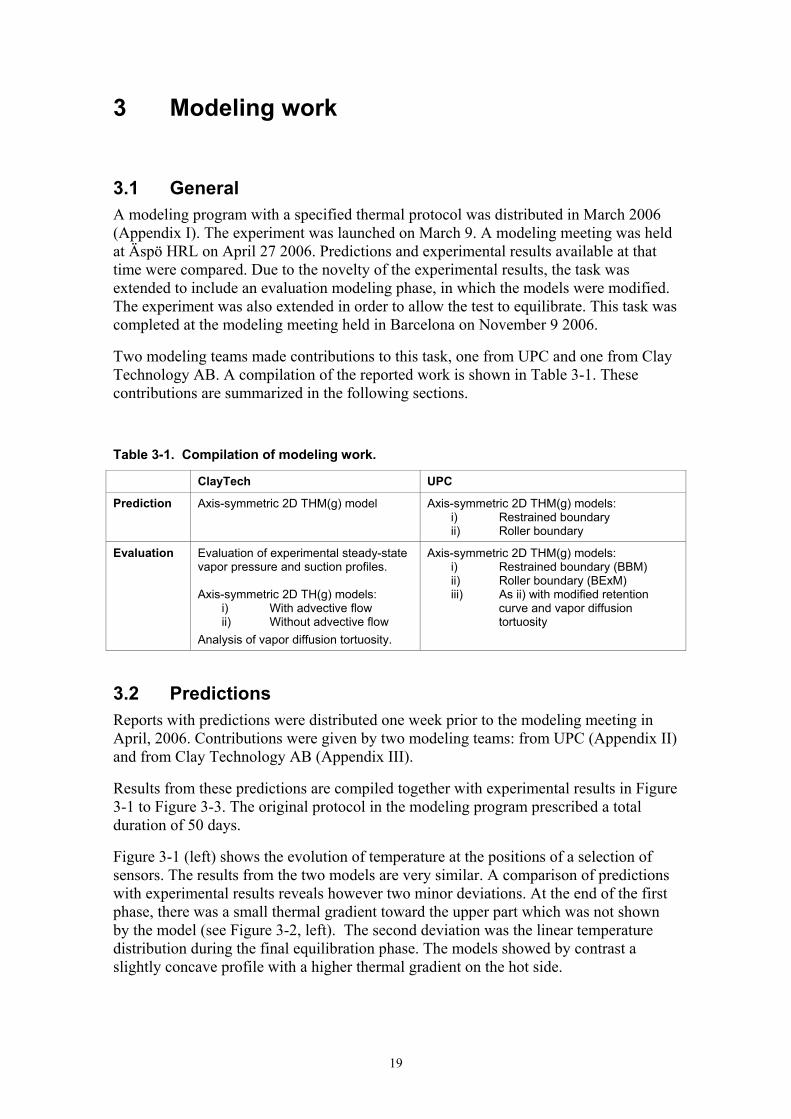
Table 2-1. Sensors location for TBT_3. Zero height is the base of bentonite specimen in contact with the lower wafer heater.

Temperature Relative humidity** Pore pressure Radial pressure

Sensor Y (mm) Sensor Y (mm) Sensor Y (mm) Sensor Y (mm)

T 0 0 HR1 22.5 PI1 52 PT1 135

T 1 2.5 HR2 37.5 PI2 84 PT2 159

T 2 18.75 HR3 52.5 PI3 116 PT3 183

T 3 35.0 HR4 72.5 PI4 148

T 4 51.25 HR5 92.5

T 5 67.5 HR6 112.5

T 6 83.75 HR7 132.5

T 7 100 HR8 152.5

T 8 116.25 HR9 172.5

T 9 132.5 HR10*** 172.5

T 10 148.75 HR11 190.0

T 11 165.0

T 12 181.25

T 13 197.5

Piston 206*

* Taking into account a 3-mm stainless-steel plate.

** A temperature measurement is associated with a humidity measurement.

*** Sensor located near the wall of the cell, in order to measure RH at the interface bentonite/casing.

19

3 Modeling work

3.1 General A modeling program with a specified thermal protocol was distributed in March 2006 (Appendix I). The experiment was launched on March 9. A modeling meeting was held at Äspö HRL on April 27 2006. Predictions and experimental results available at that time were compared. Due to the novelty of the experimental results, the task was extended to include an evaluation modeling phase, in which the models were modified. The experiment was also extended in order to allow the test to equilibrate. This task was completed at the modeling meeting held in Barcelona on November 9 2006.

Two modeling teams made contributions to this task, one from UPC and one from Clay Technology AB. A compilation of the reported work is shown in Table 3-1. These contributions are summarized in the following sections.

Table 3-1. Compilation of modeling work.

ClayTech UPC

Prediction Axis-symmetric 2D THM(g) model Axis-symmetric 2D THM(g) models: i) Restrained boundary ii) Roller boundary

Evaluation Evaluation of experimental steady-state vapor pressure and suction profiles. Axis-symmetric 2D TH(g) models:

i) With advective flow ii) Without advective flow

Analysis of vapor diffusion tortuosity.

Axis-symmetric 2D THM(g) models: i) Restrained boundary (BBM) ii) Roller boundary (BExM) iii) As ii) with modified retention

curve and vapor diffusion tortuosity

3.2 Predictions Reports with predictions were distributed one week prior to the modeling meeting in April, 2006. Contributions were given by two modeling teams: from UPC (Appendix II) and from Clay Technology AB (Appendix III).

Results from these predictions are compiled together with experimental results in Figure 3-1 to Figure 3-3. The original protocol in the modeling program prescribed a total duration of 50 days.

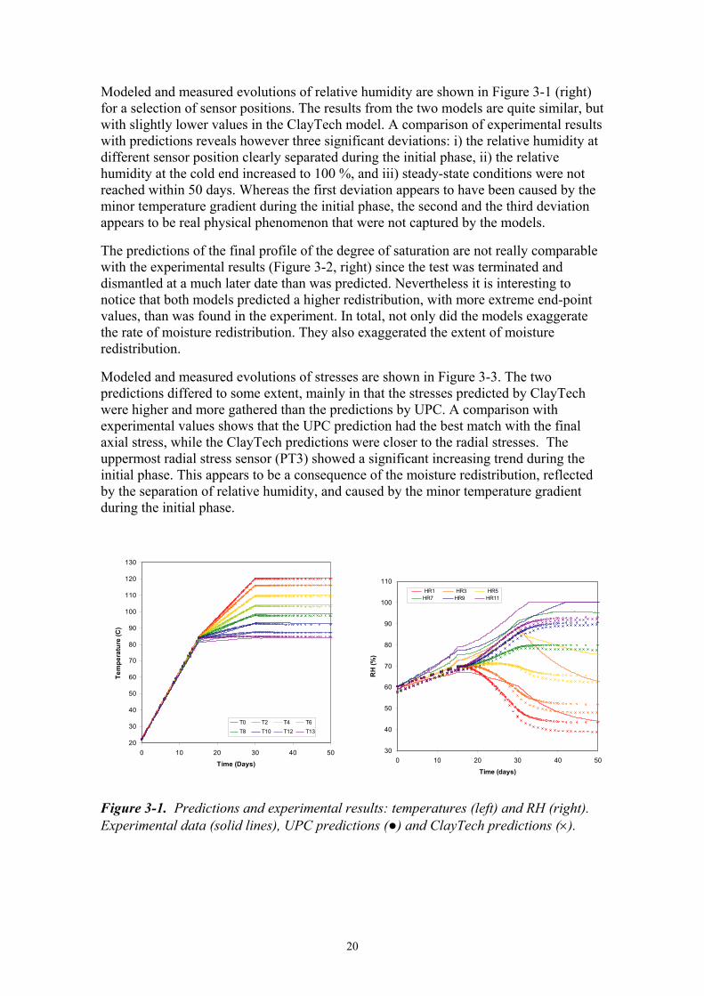
Figure 3-1 (left) shows the evolution of temperature at the positions of a selection of sensors. The results from the two models are very similar. A comparison of predictions with experimental results reveals however two minor deviations. At the end of the first phase, there was a small thermal gradient toward the upper part which was not shown by the model (see Figure 3-2, left). The second deviation was the linear temperature distribution during the final equilibration phase. The models showed by contrast a slightly concave profile with a higher thermal gradient on the hot side.

20

Modeled and measured evolutions of relative humidity are shown in Figure 3-1 (right) for a selection of sensor positions. The results from the two models are quite similar, but with slightly lower values in the ClayTech model. A comparison of experimental results with predictions reveals however three significant deviations: i) the relative humidity at different sensor position clearly separated during the initial phase, ii) the relative humidity at the cold end increased to 100 %, and iii) steady-state conditions were not reached within 50 days. Whereas the first deviation appears to have been caused by the minor temperature gradient during the initial phase, the second and the third deviation appears to be real physical phenomenon that were not captured by the models.

The predictions of the final profile of the degree of saturation are not really comparable with the experimental results (Figure 3-2, right) since the test was terminated and dismantled at a much later date than was predicted. Nevertheless it is interesting to notice that both models predicted a higher redistribution, with more extreme end-point values, than was found in the experiment. In total, not only did the models exaggerate the rate of moisture redistribution. They also exaggerated the extent of moisture redistribution.

Modeled and measured evolutions of stresses are shown in Figure 3-3. The two predictions differed to some extent, mainly in that the stresses predicted by ClayTech were higher and more gathered than the predictions by UPC. A comparison with experimental values shows that the UPC prediction had the best match with the final axial stress, while the ClayTech predictions were closer to the radial stresses. The uppermost radial stress sensor (PT3) showed a significant increasing trend during the initial phase. This appears to be a consequence of the moisture redistribution, reflected by the separation of relative humidity, and caused by the minor temperature gradient during the initial phase.

20

30

40

50

60

70

80

90

100

110

120

130

0 10 20 30 40 50

Time (Days)

Tem

pera

ture

(C)

T0 T2 T4 T6T8 T10 T12 T13

30

40

50

60

70

80

90

100

110

0 10 20 30 40 50

Time (days)

RH

(%)

HR1 HR3 HR5HR7 HR9 HR11

Figure 3-1. Predictions and experimental results: temperatures (left) and RH (right). Experimental data (solid lines), UPC predictions (●) and ClayTech predictions (×).

21

80

85

90

95

100

105

110

115

120

125

0 50 100 150 200Height (mm)

Tem

pera

ture

(C)

ClayTech UPC Experimental

Day 15

Day 50

0,2

0,3

0,4

0,5

0,6

0,7

0,8

0,9

1

0 50 100 150 200

Height (mm)

Degr

ee o

f sat

urat

ion

(-)

ClayTech- 60 dUPC - 50 dExperimental - 102 d

Figure 3-2. Predictions and experimental results: radial (left) and axial (right) stresses.

-1

0

1

2

3

4

5

6

7

0 10 20 30 40 50

Time (days)

Rad

ial s

tres

s (M

Pa)

PT1PT2PT3

0

1

2

3

4

5

0 10 20 30 40 50

Time (days)

Axi

al s

tress

(MP

a)

Figure 3-3. Predictions and experimental results: radial (left) and axial (right) stresses. Experimental data (solid lines), UPC predictions (●) and ClayTech predictions (×).

3.3 Evaluations The evaluation modeling was made after the experiment was completed and the modeling teams therefore had access to the experimental results. The contribution by the UPC team focused on improving the hydro-mechanical processes while the ClayTech team focused on the thermo-hydraulic processes.

Mechanical constitutive law

The mechanical constitutive law used for the predictions is based on the Barcelona Basic Model (BBM), and is usually employed for bentonite materials. In order to improve the model with respect to the hydro-mechanical processes, another constitutive law was used, namely the Barcelona Expansive Model (BExM). The framework for this law was defined by Gens and Alonso (1992) and was later further developed by Sanchéz (2004).

The BExM explicitly considers two pore levels: one macro- and one micro-structural level. The void ratio is therefore divided in two parts. The stress-strain relation of the macro-structural level follows BBM, while the micro-structural volumetric strain is only dependent on the mean effective stress. The interaction between structural levels is a

22

key point in the model formulation. Micro-structural deformation is considered independent of the macrostructure, but the reverse is not true. Macro-structural behavior can therefore be affected by micro-structural deformations in an irreversible way. The plastic macro-structural strains due to micro-structural strains are calculated by means of explicitly defined interaction functions.

An updated version of Code_Bright, including this new constitutive law, was used. An important effort was devoted to the definition of the parameters of the Expansive model corresponding to MX-80 bentonite, and independent laboratory experiments were used for that purpose.

Modelled and measured evolutions of stresses are shown in Figure 3-4. The agreement between these values is quite good, considering the difficulties of reproducing the mechanical behaviour of bentonite when shrinking and swelling occur in the same experiment.

Final profiles of porosity and saturation are shown in Figure 3-5. Experimental values are compared with two simulations, one using the classical BBM model and the another one using the new Expansive model. It becomes evident that the Expansive Model is able to simulate both the expansion of the bentonite in the cooler zone and the compression at the hot side using a single set of parameters.

Figure 3-4. Model and experimental evolution of stresses: axial (left) and radial (right).

0.0

25.0

50.0

75.0

100.0

125.0

150.0

175.0

200.0

0.34 0.36 0.38 0.40 0.42 0.44

Porosity

High

(mm

)

Experimental

Simulation-BBM

Simulation-BExM

Cold

Hot0.0

25.0

50.0

75.0

100.0

125.0

150.0

175.0

200.0

0.0 0.2 0.4 0.6 0.8 1.0

Saturation degree

Hig

h (m

m)

Experimental

Simulation-BBM

Simulation-BExM

Cold

Hot

Figure 3-5. Model and experimental steady-state distributions: porosity (left) and degree of saturation (right). Experimental data (symbols), BBM model (solid line) and BExM model (dotted line).

23

Moisture transport coefficients and retention properties

The evolution of vapor pressure and suction was evaluated from the experimental relative humidity and temperature data. This showed that vapor pressures tended to converge, while suction values diverged. The steady-state profiles show that the suction gradient was significant, while the corresponding vapor pressure gradient was minor (Figure 3-6).

Measured degrees of saturation and the steady-state suction values enable an evaluation of a retention curve (Figure 3-6). The suction values for the steady-state conditions are significantly lower than for free swelling samples. The experimental results indicate that the bentonite can be unsaturated under these conditions, even though the vapor is saturated. Additional tests are needed to verify this observation.

The low vapor pressure gradient at steady-state implies that the flow coefficient for vapor transport is much higher than for liquid flow. The time to reach steady-state can in addition reveal information on the values of the coefficients.

An axis-symmetric 2D TH(g) Code_Bright model was analyzed for different values of the vapor tortuosity factor (τ). Conventional values were used for the intrinsic permeability, the liquid and gas relative permeability, and the diffusion coefficient for vapor in air. A retention curve was adopted to follow the experimental results (Figure 3-6). A gas boundary with a low transfer coefficient was applied at the hot end, effectively limiting the model gas pressure to an atmospheric level.

The steady-state moisture distribution and time to reach this state was analyzed for different τ-values, and for cases with and without advective liquid flow. It was confirmed that the models without advective liquid flow in all cases reached the maximum redistribution and that the time-scale gave good agreement with experimental data for a τ-value of 0.03. For the models with advective flow, both the steady-state distribution and the time scale were dependent on the τ-value and to reach the maximum redistribution, a higher τ-value (0.15) had to be chosen. With this value the time to reach steady-state was significantly shorter than was found in the experiment.

The evolution of relative humidity in the non-advective model is compared with experimental results in Figures 3-7. The steady-state distribution of degree of saturation is also shown. The separation of the relative humidity levels and the time-scale for this are fairly well captured by the model, especially at the hot end and during the final phase. The agreement was however less good during the phase when the thermal gradient was increased, especially at the cold end. This could possibly be improved by modification of the function for the diffusion coefficient and the description of the retention properties.

24

0 50 100 150 2000

0.2

0.4

0.6

0.8

1

200

150

100

50

0

50

Vapor pressureLiquid pressure

Height (mm)

Vap

or p

ress

ure

(bar

)

Liqu

id p

ress

ure

(MPa

)

ColdHot

0.2 0.4 0.6 0.8 11

10

100

1 .103

Experimental resultsModel adaption

Degree of saturation (-)

Suct

ion

(MPa

)

Figure 3-6. Experimental steady-state profiles of vapor and liquid pressure (left). Evaluated retention curve and adapted model curve (right).

30

40

50

60

70

80

90

100

110

0 20 40 60 80 100 120

Time (days)

Rela

tive

hum

idity

(%)

Hot

Cold

Experiment Model

0,3

0,4

0,5

0,6

0,7

0,8

0 50 100 150 200

Height (mm)

Deg

ree

of s

atur

atio

n (-)

Model

Experiment

Cold

Hot

0,3

0,4

0,5

0,6

0,7

0,8

0 50 100 150 200

Height (mm)

Deg

ree

of s

atur

atio

n (-)

Model

Experiment

Cold

Hot

Figure 3-7. Model without advective flow (τ = 0.03) and experimental results. Evolution of relative humidity (left). Steady-state distribution of degree of saturation (right).

25

4 Concluding remarks

The TBT_3 Mock-up test was modeled using Code_Bright for both TH and THM analyses. This task revealed the following important results:

At steady-state, the vapor pressure exhibited a quite homogenous distribution. This indicates that the vapor pressure is the dominating potential for moisture transport at unsaturated conditions.

An evaluation of the retention properties revealed that the bentonite material can apparently be in equilibrium with saturated vapor, even though the material is not water saturated. To model the moisture redistribution with precision, the retention curve had to be modified accordingly.

It was also found that the mechanical behavior in test like TBT_3 can be well reproduced with the BExM constitutive laws, based on a double structure model (micro and macrostructure).

These results should be addressed in attempts to model the field test. In fact, they will have important implications, if they can be verified. One issue is the importance of the external water pressure for the buffer hydration, especially at temperatures above 100 ºC. For instance, in the TBT field test there have been clear indications that the hydration is influenced by the filter pressure. And in order to simulate such behaviour, it is probably necessary to apply a retention curve with a lower slope close to saturation than those usually employed. A second issue is the question of moisture redistribution during dry conditions with no water supply. The apparent retention properties evaluated from TBT_3 suggest that the actual redistribution can be less severe than those that follow from the conventional retentions curves.

27

5 References

Gatabin C., Guillot W. 2006. TBT_3 Mock-up test, Final report, July 2006. NT DPC/SCCME 06-345-A

Gens A., Alonso E.E. 1992. A framework for the behaviour of unsaturated expansive clays. Can. Geotech. J., 29, 1013-1032.

Goudarzi R., Åkesson M., Hökmark H. 2005. Äspö Hard Rock Laboratory. Temperature Buffer Test. Sensors data report (period 030326-050701) Report No:6. SKB IPR-05-20.

Sánchez M., Gens A., Guimarães L. & Olivella S. 2005. A double structure generalized plasticity model for expansive materials. Int. J. Num. and Anal. Meth. in Geomechanics 29: 751–787.

Sánchez M. 2004. Coupled Thermo-Hydro-Mechanical analysis in low permeability media. Ph.D. Thesis, Geotechnical Engineering Department, Technical University of Catalunya, Spain.

Åkesson M, 2006b. Temperature Buffer Test. Evaluation modelling - Mock-up test. IPR-06-11, Svensk Kärnbränslehantering AB.

29

Appendix 1

Clay Technology AB

Ideon Research Center

Lund, Sweden

TBT_3 - Predictive modeling program

March, 2006

Mattias Åkesson

Harald Hökmark

31

Contents

1 TBT_3 Mockup experiment 33 1.1 Background 33 1.2 Time table 33 1.3 Experimental setup 33 1.4 Thermal protocol 34 1.5 Instrumentation 35

2 Suggested scope and requested output 37

33

1 TBT_3 Mockup experiment

1.1 Background Within the framework of the TBT evaluation modeling task force, it has been decided to emphasize the initial thermo-hydraulic condition around the lower heater in the TBT test. Of special interest are the phenomena of desaturation and the role of temperature gradients and temperature levels.

This problem was addressed through the TBT_2 mockup test, which was carried out during 2005. The approach was two-parted, with a mockup test combined with a predictive modeling task. The results were presented at the TBT modeling meeting in Barcelona on October 27th 2005.

Due to an observed leak of heat in the midsection of the TBT_2 setup, an improved experimental design has been developed for the follow-up TBT_3 test. This will also consist of a combined experimental and blind predictive modeling work.

1.2 Time table The mockup test is scheduled to start in the beginning of March 2006. The requested time for experimental and modeling results is April 20, which is one week prior to the modeling meeting at Äspö, at which comparisons and evaluations will be presented.

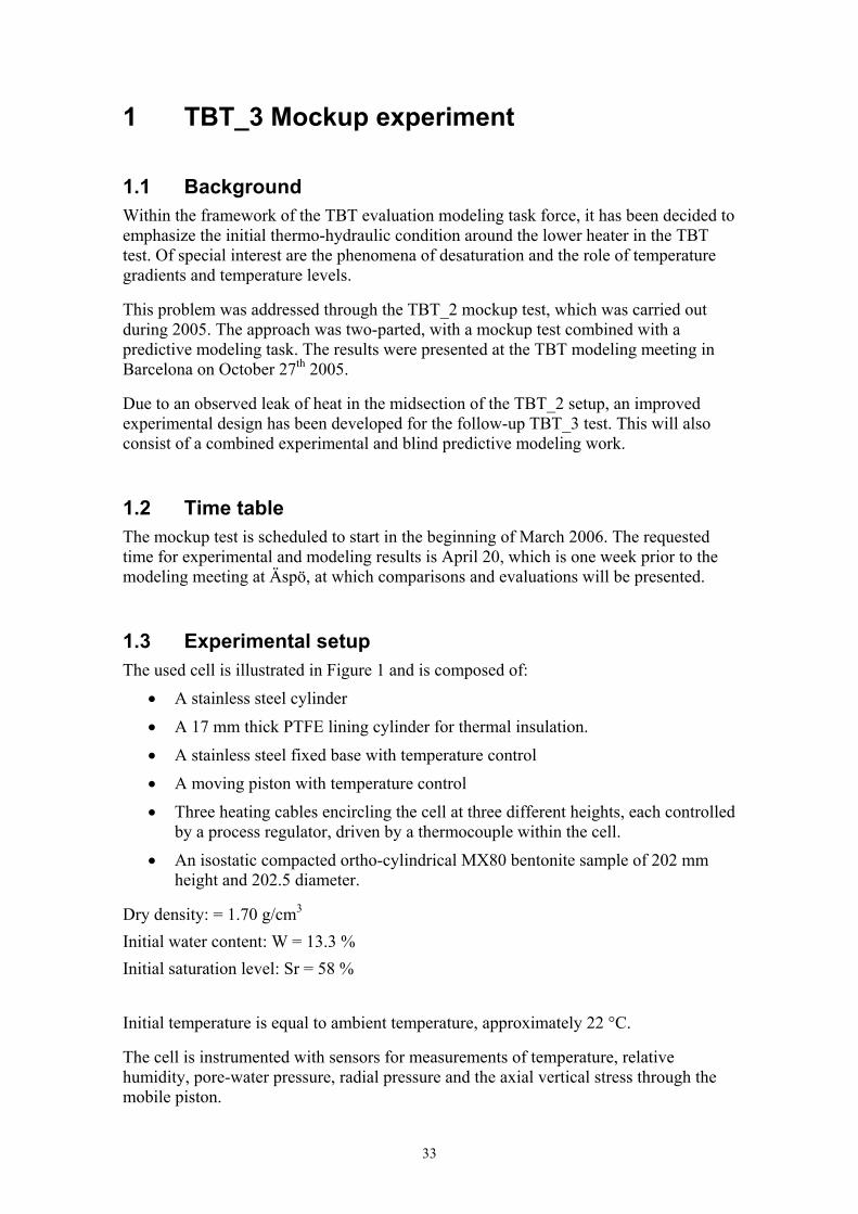
1.3 Experimental setup The used cell is illustrated in Figure 1 and is composed of:

• A stainless steel cylinder • A 17 mm thick PTFE lining cylinder for thermal insulation. • A stainless steel fixed base with temperature control • A moving piston with temperature control

• Three heating cables encircling the cell at three different heights, each controlled by a process regulator, driven by a thermocouple within the cell.

• An isostatic compacted ortho-cylindrical MX80 bentonite sample of 202 mm height and 202.5 diameter.

Dry density: = 1.70 g/cm3 Initial water content: W = 13.3 % Initial saturation level: Sr = 58 % Initial temperature is equal to ambient temperature, approximately 22 °C.

The cell is instrumented with sensors for measurements of temperature, relative humidity, pore-water pressure, radial pressure and the axial vertical stress through the mobile piston.

34

Peripheral temperature control Hot side

temperature control

Cold side temperature control


temperature control


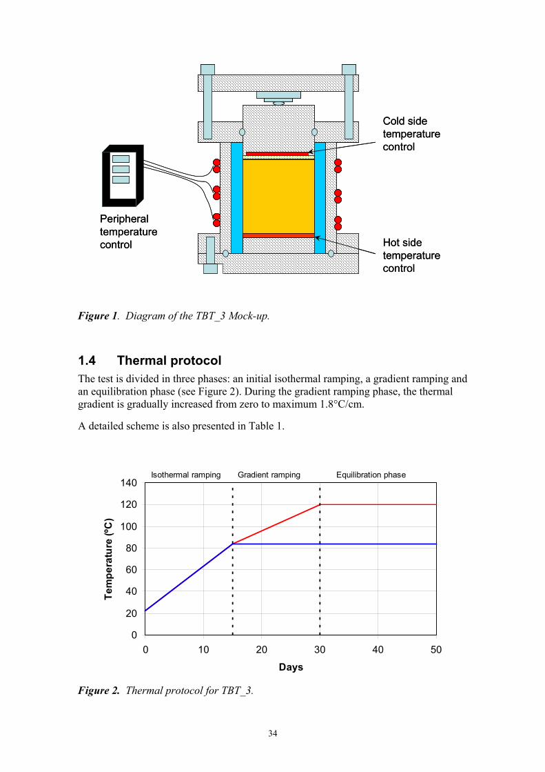
Figure 1. Diagram of the TBT_3 Mock-up.

1.4 Thermal protocol The test is divided in three phases: an initial isothermal ramping, a gradient ramping and an equilibration phase (see Figure 2). During the gradient ramping phase, the thermal gradient is gradually increased from zero to maximum 1.8°C/cm.

A detailed scheme is also presented in Table 1.

0

20

40

60

80

100

120

140

0 10 20 30 40 50

Days

Tem

pera

ture

(ºC

)

Isothermal ramping Gradient ramping Equilibration phase

Figure 2. Thermal protocol for TBT_3.

35

Table 1. Details of thermal protocol.

Day Temperature (Hot face)

Temperature (Cold face)

0 22 22 15 84 84 30 120 84 >50 120 84

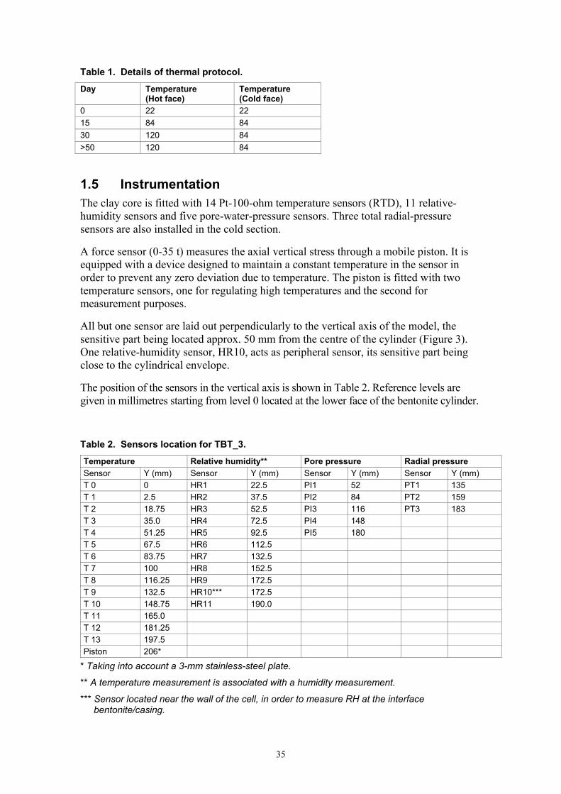
1.5 Instrumentation The clay core is fitted with 14 Pt-100-ohm temperature sensors (RTD), 11 relative-humidity sensors and five pore-water-pressure sensors. Three total radial-pressure sensors are also installed in the cold section.

A force sensor (0-35 t) measures the axial vertical stress through a mobile piston. It is equipped with a device designed to maintain a constant temperature in the sensor in order to prevent any zero deviation due to temperature. The piston is fitted with two temperature sensors, one for regulating high temperatures and the second for measurement purposes.

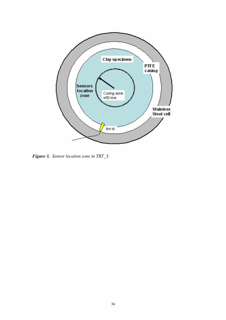
All but one sensor are laid out perpendicularly to the vertical axis of the model, the sensitive part being located approx. 50 mm from the centre of the cylinder (Figure 3). One relative-humidity sensor, HR10, acts as peripheral sensor, its sensitive part being close to the cylindrical envelope.

The position of the sensors in the vertical axis is shown in Table 2. Reference levels are given in millimetres starting from level 0 located at the lower face of the bentonite cylinder.

Table 2. Sensors location for TBT_3.

Temperature Relative humidity** Pore pressure Radial pressure Sensor Y (mm) Sensor Y (mm) Sensor Y (mm) Sensor Y (mm) T 0 0 HR1 22.5 PI1 52 PT1 135 T 1 2.5 HR2 37.5 PI2 84 PT2 159 T 2 18.75 HR3 52.5 PI3 116 PT3 183 T 3 35.0 HR4 72.5 PI4 148 T 4 51.25 HR5 92.5 PI5 180 T 5 67.5 HR6 112.5 T 6 83.75 HR7 132.5 T 7 100 HR8 152.5 T 8 116.25 HR9 172.5 T 9 132.5 HR10*** 172.5 T 10 148.75 HR11 190.0 T 11 165.0 T 12 181.25 T 13 197.5 Piston 206*




36

Figure 3. Sensor location zone in TBT_3.

37

2 Suggested scope and requested output

The mockup test emphasizes the thermo-hydraulic phenomena of desaturation. Modeling results regarding temperature, relative humidity, radial stress and axial stress are to be presented as history plots for each individual sensor position. The time resolution of the history plots should not be more than one day.

Models should be run until steady-state condition is reached. This may require more time than the 50 days prescribed by the protocol.

Ideally, the test can be described as a 1D problem. If, however, the problem is modeled as 2D, the results should be presented as follows:

• Since temperature and RH sensors are located off axis, modeling results for these should be given for a radius of 50 mm.

• Modeling results for the peripheral sensor, i.e. for radial stresses and RH (sensor HR10), should be given for a radius of 100 mm.

• The axial stress can be given as an average over the top surface.

Finally, model results should also be given for the steady-state condition regarding degree of saturation. This should be given as a scan-line along the central axis, in order to make comparisons with water ratio measurements after dismantling.

39

Appendix 2

TBT_3 – Predictive Modelling Program

Simulation of TBT_3 Mockup Experiment

ENRESA Contribution

April 2006

A. Ledesma, A. Jacinto

UPC, Barcelona, Spain

M. Velasco

DM Iberia, Madrid, Spain

41

Contents

1 Introduction 43

2 Test description and input data 45 2.1 Experimental setup 45 2.2 Parameters considered 46 Thermal Problem 46

Thermal conductivity )( mKWλ 46 Specific heat 46

Hydraulic Problem 47 Retention curve 47 Intrinsic permeability 47 Liquid relative permeability 47 Gas relative permeability 47 Molecular diffusion of vapour 47 Molecular diffusion of dissolved air 47

Mechanical Problem 48 Thermal elasticity 48 Barcelona Basic Model (BBM) 48

Temperature 48 Mechanical 48

3 Numerical results 51

4 Influence of Mechanical Boundary conditions 55

5 Concluding Remarks 57

43

1 Introduction

This report presents the modelling work performed by the team coordinated by ENRESA (Spain) regarding the simulation of the “TBT_3 Mockup Experiment” performed at CEA (France). The guidelines considered in this simulation were defined in a document by M. Åkesson & H. Hökmark (Clay Technology, March 2006), entitled “TBT_3 Predictive Modeling Program”. That report presented the protocol of the experiment and the variables expected from this modelling exercise. As indicated there, TBT_3 test was designed to improve the experimental setup of TBT_2, which presented a leak of heat in the midsection of the sample. A blind predictive process, similar to the one performed with TBT_2 has been followed in this new case.

As in previous simulation exercises, we have used the information provided in that report and in previous documents of the TBT project in order to define the parameters and the boundary conditions of the experiment. When a parameter was not known in advance, a reasonable value, based on our previous experience, was adopted for the simulation.

The Spanish participation in this project is coordinated by F. Huertas (ENRESA), and includes groups from UPC and from DM Iberia. In particular, the simulation work described in this report has been developed by the UPC group (A. Ledesma, A. Jacinto), with collaboration of M. Velasco from DM Iberia.

The code CODE_BRIGHT has been used in all cases, as in the previous simulations performed by the group. Due to the experience obtained with the TBT_2 simulation programme, the number of numerical analyses performed for this TBT_3 case has been reduced considerably. Two specific models were selected for a final comparison, being similar in parameters and boundary conditions except for the mechanical restrictions in the sample surface. In all cases a 2D – axisymmetric geometry was adopted.

Section two presents a brief explanation of the experiment and the material properties adopted in the simulations. A description of the conditions of both final models is also included. Section three presents the requested output regarding the blind prediction of THM variables in the test. An additional section (section four) includes some comments about the differences in terms of mechanical variables between those final models above mentioned. The report ends up with some concluding remarks about this simulation and the future work.

45

2 Test description and input data

2.1 Experimental setup

Details of the experimental setup can be found in the report by Clay Technology already mentioned. For consistency figure 1 presents a sketch of the geometry obtained from that report.


temperature control



temperature control


Figure 1. Diagram of the TBT_3 Mock-up (from Clay Technology, 2006).

The bentonite sample is a cylinder 202 mm height and 202.5 mm diameter subjected to a thermal gradient that follows the protocol described in figure 2. The MX-80 bentonite has the following basic properties:

- Dry density: 1.70 g/cm3 - Initial water content: 13.3% - Initial saturation level: around 58% - Initial temperature: around 22ºC

The cell has been instrumented in order to measure the temporal evolution of temperature, RH, liquid pressure and stresses.

46

0

20

40

60

80

100

120

140

0 10 20 30 40 50

Days

Tem

pera

ture

(ºC

)


Figure 2. Thermal protocol for the experiment: temperature at “hot” and “cold” surfaces. (Clay Technology, 2006).

2.2 Parameters considered Material properties for the bentonite have been adopted from the previous experience in modelling THM behaviour of MX-80. Note that despite the amount of work already developed, the information available regarding the mechanical properties of MX-80 bentonite is still very limited. In this case we have adopted some parameters based on our previous experience. Main parameters follow:

Thermal Problem

Thermal conductivity )( mKWλ ll S

drySsat

−⋅= 1λλλ

dryλ = 0.3 satλ = 1.3

Specific heat

c (J/kg K)= 1091

47

Hydraulic Problem

Retention curve

m

m

lglg

rlls

rlle S

PPP

PPSSSS

S ⎟⎟⎠

⎞⎜⎜⎝

⎛ −−

⎥⎥⎥

⎦

⎤

⎢⎢⎢

⎣

⎡

⎟⎟⎠

⎞⎜⎜⎝

⎛ −+=

−−

=

−

−

111

1

0

β

β

0P (MPa) = 30.6 β = 0.3 mS (MPa) = 600 m = 1.1

Intrinsic permeability

30

20

2

3

0)1(

)1( φφ

φφ −−

= kk

)( 20 mk = 3.6x10-21 0φ = 0.397 ( e = 0.659)

Liquid relative permeability λerl ASk =

A = 1 λ = 3

Gas relative permeability λegrl ASk =

A = 2.184x108 λ = 4.17

Molecular diffusion of vapour ( )

⎟⎟⎠

⎞⎜⎜⎝

⎛ +=

g

nvm P

TDD 15.273τ

D = 5.9x10-6 n = 2.3 τ = 1

Molecular diffusion of dissolved air

( )⎟⎟⎠⎞

⎜⎜⎝

⎛+

−=

TRQDDv

m 15.273expτ

D = 1.1x10-4 n = 24530 τ = 1.0x10-5

48

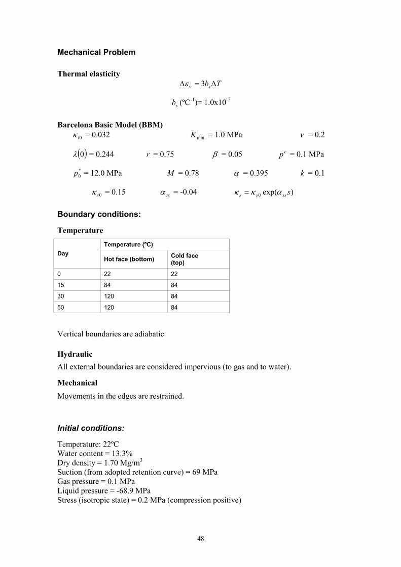
Mechanical Problem

Thermal elasticity Tbsv Δ=Δ 3ε

sb (ºC-1)= 1.0x10-5

Barcelona Basic Model (BBM) 0iκ = 0.032 minK = 1.0 MPa ν = 0.2

( )0λ = 0.244 r = 0.75 β = 0.05 cp = 0.1 MPa

*0p = 12.0 MPa M = 0.78 α = 0.395 k = 0.1

0sκ = 0.15 ssα = -0.04 )exp(0 sssss ακκ =

Boundary conditions:

Temperature

Temperature (ºC) Day

Hot face (bottom) Cold face (top)

0 22 22

15 84 84

30 120 84

50 120 84

Vertical boundaries are adiabatic

Hydraulic All external boundaries are considered impervious (to gas and to water).

Mechanical Movements in the edges are restrained.

Initial conditions:

Temperature: 22ºC Water content = 13.3% Dry density = 1.70 Mg/m3

Suction (from adopted retention curve) = 69 MPa Gas pressure = 0.1 MPa Liquid pressure = -68.9 MPa Stress (isotropic state) = 0.2 MPa (compression positive)

49

The set of parameters presented corresponds to the case shown in next section. Another simulation was also considered during the final stage of this modelling work. The only difference between those “final” models was the mechanical boundary condition in the sample surface. The case presented in next section, assumed as “proposed solution”, was computed considering zero displacements on that surface, that is, no relative displacement between sample surface and PTFE casing was allowed. The alternative case was computed assuming free movement in the direction of the contact between mould and sample surface, and restriction in a direction perpendicular to the contact only.

It should be stressed that both “final models” gave in practice similar results in terms of TH variables. However, a substantial difference was found in the evolution of the stresses. The model with zero-movement boundary condition provided with a level of stresses more consistent with the measurements obtained in previous test TBT-2. When boundaries had a free displacement condition, the computed stresses resulted in very low values. Most probably the actual behaviour of the test will be somehow in mixed conditions, but this is difficult to predict in advance. Some comments on the reliability of this assumption have been included in section 4.

Obviously, another procedure to simulate high stress levels is to change the mechanical parameters used in the model. In this case, however, we have preferred to use the same set of parameters for the whole sample and for the whole duration of the experiment. Mechanical parameters have been obtained from the interpretation of simple and independent experiments performed on MX-80 bentonite (i.e., oedometer tests, swelling pressure tests and free swelling tests), and reported in the literature (i.e. Villar, 2005). It should be recognized, however, that this information is limited, and therefore, mechanical parameters and the BBM model itself should be improved in future simulations as soon as new information is gained from this modelling exercises.

51

3 Numerical results

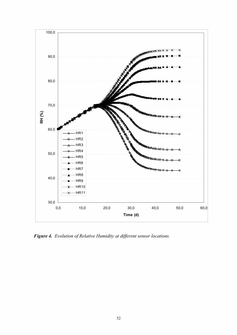
The results obtained in the proposed final case are included in this section. Figure 3 shows the evolution of temperature against time at different sensor locations. Figure 4 presents the same evolution for Relative Humidity.

20,0

40,0

60,0

80,0

100,0

120,0

140,0

0,0 10,0 20,0 30,0 40,0 50,0 60,0

Time (d)

Tem

pera

ture

(ºC

)

T0

T1

T2

T3

T4

T5

T6

T7

T8

T9

T10

T11

T12

T13

Piston

Figure 3. Temperature evolution at different sensor locations.

52

30,0

40,0

50,0

60,0

70,0

80,0

90,0

100,0

0,0 10,0 20,0 30,0 40,0 50,0 60,0

Time (d)

RH

(%)

HR1

HR2

HR3

HR4

HR5

HR6

HR7

HR8

HR9

HR10

HR11

Figure 4. Evolution of Relative Humidity at different sensor locations.

53

The results show a 1-Dimensional pattern regarding TH variables, as the model preserves essentially this symmetry. The experiment is assumed “closed” regarding water and gas. In fact, gas could escape from the sample because it is difficult in practice to guarantee gas tightness in the cell. However, the simulations show that gas pressure is always below 0.2 MPa (starting form a 0.1 MPa initial value), and it is considered that the effect of gas is not relevant in the resulting THM variables measured in the test. Values close to the atmospheric pressure should therefore be expected in the experiment, in the range 0.1 – 0.2 MPa.

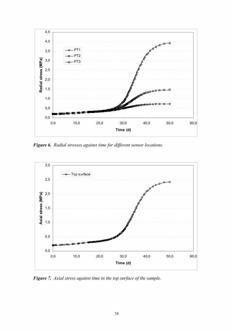
Figure 5 presents scan-lines of degree of saturation along the central axis of the sample, as requested by the modelling program. Finally, radial stresses are presented in figure 6, and axial stresses in figure 7.

0,0

50,0

100,0

150,0

200,0

0,2 0,3 0,4 0,5 0,6 0,7 0,8 0,9 1,0

Saturation degree

Hei

ght (

mm

)

0 d

15 d

22 d

30 d

35 d

50 d

Figure 5. Saturation degree along the central axis of the sample for different times.

54

0,0

0,5

1,0

1,5

2,0

2,5

3,0

3,5

4,0

4,5

0,0 10,0 20,0 30,0 40,0 50,0 60,0

Time (d)

Rad

ial s

tress

(MP

a)

PT1

PT2

PT3

Figure 6. Radial stresses against time for different sensor locations.

0,0

0,5

1,0

1,5

2,0

2,5

3,0

0,0 10,0 20,0 30,0 40,0 50,0 60,0

Time (d)

Axi

al s

tress

(MP

a)

Top surface

Figure 7. Axial stress against time in the top surface of the sample.

55

4 Influence of Mechanical Boundary conditions

A second “final example” has been simulated considering that sample boundaries have free movement in the direction of the contact mould-bentonite (that is, roller boundaries). This is in fact a typical boundary condition in these kinds of simulations, but it was found that the level of stresses obtained in this manner was well below measured values. Figures 8 and 9 show the radial and axial stresses obtained using roller boundaries and keeping the same parameters as in the case presented in previous section. TH variables did not change substantially with respect to that case in section 3.

It should be pointed out that radial stresses have the same order of magnitude in both simulations, but axial stresses are very low when rollers are considered in the boundaries. It is difficult to say in advance if in the real experiment the contact between bentonite and PTFE casing is smooth or not. Most probably that will change during the experiment, and it will depend on the tangential and the normal stresses developed at that contact. In order to get some insight into the behaviour of that contact, the reactions in the vertical boundaries of the proposed case of section 3 (zero displacements at the boundaries) have been computed as well. The ratio “tangential stress / normal stress” at the boundary has been plotted in figure 10 as the tangent of a contact angle. Note that before day 30th, this contact angle is below 15º in the sample boundary, a value that could be considered low. A smooth contact may still provide a contact angle close to that value, although this is difficult to assure without practical measurements of this friction between bentonite and the PTFE casing. Therefore, it is considered that the actual test will behave in a mixed manner regarding this aspect of mechanical boundary conditions.

0,0

0,5

1,0

1,5

2,0

2,5

0,0 10,0 20,0 30,0 40,0 50,0 60,0

Time (d)

Rad

ial s

tres

s (M

Pa) PT1

PT2PT3

Figure 8. Radial stresses for the analysis considering rollers as mechanical boundary condition.

56

0,0

0,1

0,2

0,3

0,4

0,5

0,6

0,0 10,0 20,0 30,0 40,0 50,0 60,0

Time (d)

Axi

al s

tres

s (M

Pa)

Top surface

Figure 9. Axial stresses on the top of the sample, in the analysis considering rollers as mechanical boundary condition.

0,0

50,0

100,0

150,0

200,0

0,0 5,0 10,0 15,0 20,0 25,0 30,0 35,0 40,0

δ (º)

Hei

ght (

mm

)

0 d

15 d

22 d

30 d

35 d

50 d

Figure 10. Ratio shear stress/normal stress at the contact boundary between bentonite and PTFE casing, expressed as the tangent of a contact angle.

57

5 Concluding Remarks

This report includes the results of the predictive modelling programme of the TBT_3 experiment performed by the group coordinated by ENRESA. The definition of the models and the parameters used in the computations follow the guidelines of the document by Clay Technology (2006).

The output of the simulation work has been presented in section 3, and includes time evolution of temperature, relative humidity and stresses (radial & axial). An additional case which keeps in fact all the parameters, but changes the mechanical boundary conditions has been presented in section 4. The idea was to point out the effect of mechanical boundary conditions on the stress levels in the bentonite. A discussion about the validity of the hypothesis considered has been included as well.

It is believed that the prediction of TH variables is reasonably performed, according to the success of previous modelling exercises. However, the prediction of mechanical variables (i.e. stresses) is still far from being satisfactory, maybe due to some uncertainties regarding modelling parameters and boundary conditions. This work and future exercises may provide with new information for future developments regarding this aspect.

59

References

Clay Technology (2006) – (M. Åkesson, H. Hökmark). TBT_3 – Predictive Modeling Program, March 2006.

Villar M.V. (2005). MX-80 Bentonite. Thermo-Hydro-Mechanical Characterisation Performed at CIEMAT in the Context of the Prototype Project. Informes Técnicos Ciemat. 1053. Febrero, 2005.

61

Appendix 3

Clay Technology AB


Lund, Sweden

TBT_3 Mock-up predictions

April, 2006

Mattias Åkesson

63

Contents

1 Background 65

2 TBT_3 Mock-up experiment 67 2.1 General 67 2.2 Experimental setup 67 2.3 Thermal protocol 67 2.4 Instrumentation 69

3 Predictive modeling 71 3.1 Model description 71

3.1.1 Model geometry 71 3.1.2 Initial and boundary conditions 72 3.1.3 Thermo-hydraulic parameters. 72 3.1.4 Mechanical parameters 74

3.2 Results 75 3.2.1 Base case 75 3.2.2 Influence of mechanical couplings 77

4 Final remarks 79

5 References 81

65

1 Background

Within the framework of the TBT evaluation modeling task force, it has been decided to emphasize the initial thermo-hydraulic condition around the lower heater in the TBT test. Of special interest are the phenomena of desaturation and the role of temperature gradients and temperature levels.


Due to an observed leak of heat in the midsection of the TBT_2 setup, an improved experimental design has been developed for the follow-up TBT_3 test. This will also consist of a combined experimental and blind predictive modeling work.

A description of the test and a guideline with requested modeling results was given in a modeling program /Åkesson and Hökmark, 2006/. The test was launched on March 9th 2006.

67

2 TBT_3 Mock-up experiment

2.1 General The mock-up test was planned and designed at the CEA laboratory in Saclay, France. The basic idea is to subject a confined sample of MX80 bentonite material to thermal gradients similar to those around the lower heater in the TBT field experiment, and to monitor the development of temperatures, relative humidities and stresses during a well-defined sequence of thermal loading.

2.2 Experimental setup The used cell is illustrated in Figure 1 and is composed of:

• A stainless steel cylinder

• A 17 mm thick PTFE lining cylinder for thermal insulation.

• A stainless steel fixed base with temperature control

• A moving piston with temperature control

• Three heating cables encircling the cell at three different heights, each controlled by a process regulator, driven by a thermocouple within the cell.

• An isostatic compacted ortho-cylindrical MX80 bentonite sample of 202 mm height and 202.5 diameter.

Initial temperature is equal to ambient temperature, approximately 22 °C.

The cell is instrumented with sensors for measurements of temperature, relative humidity, pore-water pressure, radial pressure and the axial vertical stress through the mobile piston.

2.3 Thermal protocol The test is divided in three phases: an initial isothermal ramping, a gradient ramping and an equilibration phase (see Figure 2). During the gradient ramping phase, the thermal gradient is gradually increased from zero to maximum 1.8°C/cm.

68


temperature control



temperature control


Figure 1. Diagram of the TBT_3 Mock-up.

0

20

40

60

80

100

120

140

0 10 20 30 40 50

Days

Tem

pera

ture

(ºC

)


Figure 2. Thermal protocol for TBT_3.

69

2.4 Instrumentation The clay core is fitted with 14 Pt-100-ohm temperature sensors (RTD), 11 relative-humidity sensors and five pore-water-pressure sensors. Three total radial-pressure sensors are also installed in the cold section.

A force sensor (0-35 t) measures the axial vertical stress through a mobile piston. It is equipped with a device designed to maintain a constant temperature in the sensor in order to prevent any zero deviation due to temperature. The piston is fitted with two temperature sensors, one for regulating high temperatures and the second for measurement purposes.

All but one sensor are laid out perpendicularly to the vertical axis of the model, the sensitive part being located approx. 50 mm from the centre of the cylinder. One relative-humidity sensor, HR10, acts as peripheral sensor, its sensitive part being close to the cylindrical envelope.

The position of the sensors in the vertical axis is shown in Table 1. Reference levels are given in millimetres starting from level 0 located at the lower face of the bentonite cylinder.

Table 1. Sensors location for TBT_3.

Temperature Relative humidity** Pore pressure Radial pressure

Sensor Y (mm) Sensor Y (mm) Sensor Y (mm) Sensor Y (mm)

T 0 0 HR1 22.5 PI1 52 PT1 135

T 1 2.5 HR2 37.5 PI2 84 PT2 159

T 2 18.75 HR3 52.5 PI3 116 PT3 183

T 3 35.0 HR4 72.5 PI4 148

T 4 51.25 HR5 92.5 PI5 180

T 5 67.5 HR6 112.5

T 6 83.75 HR7 132.5

T 7 100 HR8 152.5

T 8 116.25 HR9 172.5

T 9 132.5 HR10*** 172.5

T 10 148.75 HR11 190.0

T 11 165.0

T 12 181.25

T 13 197.5

Piston 206*




71

3 Predictive modeling

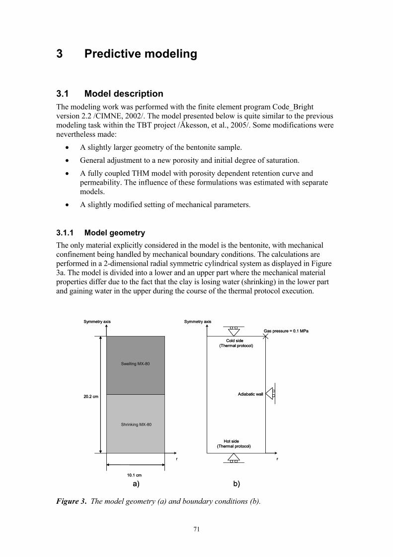
3.1 Model description The modeling work was performed with the finite element program Code_Bright version 2.2 /CIMNE, 2002/. The model presented below is quite similar to the previous modeling task within the TBT project /Åkesson, et al., 2005/. Some modifications were nevertheless made:

• A slightly larger geometry of the bentonite sample. • General adjustment to a new porosity and initial degree of saturation. • A fully coupled THM model with porosity dependent retention curve and

permeability. The influence of these formulations was estimated with separate models.

• A slightly modified setting of mechanical parameters.

3.1.1 Model geometry The only material explicitly considered in the model is the bentonite, with mechanical confinement being handled by mechanical boundary conditions. The calculations are performed in a 2-dimensional radial symmetric cylindrical system as displayed in Figure 3a. The model is divided into a lower and an upper part where the mechanical material properties differ due to the fact that the clay is losing water (shrinking) in the lower part and gaining water in the upper during the course of the thermal protocol execution.

10.1 cm

Symmetry axis

r

20.2 cm

Swelling MX-80

Shrinking MX-80

Cold side(Thermal protocol)

Symmetry axis

r

Gas pressure = 0.1 MPa

Hot side(Thermal protocol)

Adiabatic wall

a) b)10.1 cm

Symmetry axis

r

20.2 cm

Swelling MX-80

Shrinking MX-80


Symmetry axis

r



Adiabatic wall

a) b)

Figure 3. The model geometry (a) and boundary conditions (b).

72

3.1.2 Initial and boundary conditions Modeling was performed for a system with hydraulically closed boundaries. The system was modeled with a gas boundary at atmospheric pressure at the upper circumference (Figure 3b), while the gas flux was prohibited on the remaining boundaries.

The modeling of the system with a gas boundary implies that the gas pressure is basically atmospheric throughout the bentonite sample. This condition promotes the vapor diffusion and enhances the water redistribution. A completely isolated system would instead result in a lesser redistribution. The question whether the system is gas tight or not is therefore crucial for the prediction of the process. The choice of a gas boundary in this model was justified by the results from the pore pressure measurements from the previous TBT_2 test, which essentially indicated atmospheric conditions.

The heating of the sample was modeled using time-dependent temperature boundary conditions on the top and bottom boundaries as described in the modeling program (c.f. Figure 2). The vertical boundaries were adiabatic.

All boundaries were roller boundaries, i.e. mechanically fixed in the normal direction.

The used initial conditions are shown in Table 3.

3.1.3 Thermo-hydraulic parameters The thermo-hydraulic parameter values are shown in Table 2. The adjustments of these parameters in relation to the previous task are commented below.

Table 2. Thermo-hydraulic parameters.

Initial Saturation level Sini = 58 % Initial water ratio wini = 13.3 % Dry density ρdry = 1.70 g/cm3 Solid phase density ρs = 2.78 g/cm3 Porosity n = 0.388 - Void ratio e = 0.635 - Intrinsic permeability (isotropic) k = 2.5·10-21 m2 Liquid relative permeability kr = Sr

3 - Gas phase relative permeability krg = 108(1-Sr)4 - Solid state specific heat Cs = 800 J/(kg·K) Heat conductivity λ = 0.3·(1-Sr) +1.2·Sr W/(m·K) Tortuosity for vapor diffusion τ = 0.3 - Porosity dependent van Genuchten model: P0 30.5 MPa MPa λ 0.35 - a 17 - b 4 -

σ0 0.072 N/m

73

Table 3. Initial conditions.

Porosity (-)

Gas pressure (MPa)

Liquid pressure (MPa)

Temperature (°C)

Stresses (MPa)

0.388 0.1 -72 22 0.2/0.2/0.2 (compression)

Porosity and initial degree of saturation

Information on water content and dry density, provided by CEA, corresponds to a porosity of 0.388, a void ratio of 0.635 and an initial degree of saturation of 58 %.

Retention curve parameters

Parameters for the porosity dependent van Genuchten model of the retention curve (Eq. 1) were estimated from experimental RH vs. water mass ratio data /Dueck, 2004/. These data series, corresponding respectively to an initial water mass ratio of 8 and 17.5%, were linearly interpolated to the present value of w=13.3%. The experimental data and model retention curves are shown in Figure 4 for five different void ratios.

( ) ( ))(4exp35.0)()(17exp5.30)(1 000

11

nnnnnnPPsSro

−⋅⋅=−⋅⋅=⎟⎟⎟

⎠

⎞

⎜⎜⎜

⎝

⎛

⎟⎟⎠

⎞⎜⎜⎝

⎛+=

−

−

λ

λ

λ

(1)

0.1 0.2 0.3 0.4 0.5 0.6 0.7 0.8 0.910

100

1 .103

Data: e=0.55Data: e=0.60Data: e=0.635Data: e=0.70Data: e=0.75Model: e=0.55Model: e=0.60Model: e=0.635Model: e=0.70Model: e=0.75


Suct

ion

(MPa

)

Figure 4. Experimental data (interpolated to w=13.3%) and model retention curves for five different void ratios.

74

Intrinsic permeability

The intrinsic permeability for the initial e of 0.635 was set to 2.5 ·10-21 m2 according to data from /Börgesson et al., 1999/. Moreover, the porosity dependence implemented in Code_Bright was utilized in the base case.

3

0

20

0 11

⎟⎟⎠

⎞⎜⎜⎝

⎛⋅⎟

⎠⎞

⎜⎝⎛

−−

⋅=nn

nn

kk (2)

3.1.4 Mechanical parameters The mechanical parameters used (Table 4) were adopted from the model of the earlier CEA mockup test studied within the EBS Task Force /Birgersson et al., 2005/. The αsp value for the swelling material was modified from -0.21 to -0.23 in order to obtain axial stresses with the same magnitude (∼3 MPa) as in TBT_2. No yield surface was applied.

Table 4. Mechanical equations and associated parameters.

Thermo-elastoplastic constitutive law (elastic domain)

dTTs

dsesp

pdp

esd sie )2(

1.01),(

1)(

20 Δ++++

++

= αακκεν

⎥⎦

⎤⎢⎣

⎡⎟⎠⎞

⎜⎝⎛ +

++=1.0

1.0ln1)( 0sss ilsiii αακκ

s

refspss

sseppsp αακκ

⎥⎥⎦

⎤

⎢⎢⎣

⎡⎟⎟⎠

⎞⎜⎜⎝

⎛+= ln1),( 0

dε = Volumetric strain (-) p = Net mean stress (MPa) s = Suction (MPa) T = Temperature (°C)

Swelling:

⎥⎦

⎤⎢⎣

⎡⎟⎠⎞

⎜⎝⎛ +

⋅−⋅+⋅=1.0

1.0ln15.00009.0125.0)( sssiκ

⎥⎦

⎤⎢⎣

⎡⎟⎠⎞

⎜⎝⎛⋅−⋅=

1.0ln23.0128.0)( ppsκ

Kmin = 10 MPa; ν=0.4

α0 =3·10-6; α2 = 0

Shrinking:

02.0)( =siκ

ss es 04.016.0)( −⋅=κ

Kmin = 10 MPa; ν=0.2

α0 =3·10-6; α2 = 0

75

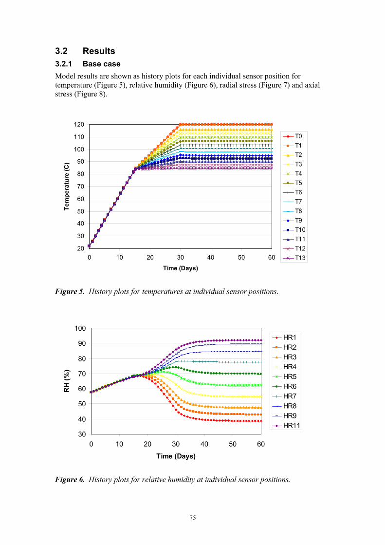
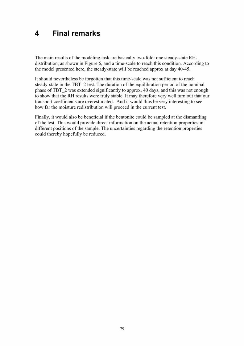
3.2 Results 3.2.1 Base case Model results are shown as history plots for each individual sensor position for temperature (Figure 5), relative humidity (Figure 6), radial stress (Figure 7) and axial stress (Figure 8).

20

30

40

50

60

70

80

90

100

110

120

0 10 20 30 40 50 60

Time (Days)

Tem

pera

ture

(C)

T0T1T2T3T4T5T6T7T8T9T10T11T12T13

Figure 5. History plots for temperatures at individual sensor positions.

30

40

50

60

70

80

90

100

0 10 20 30 40 50 60

Time (Days)

RH

(%)

HR1HR2HR3HR4HR5HR6HR7HR8HR9HR11

Figure 6. History plots for relative humidity at individual sensor positions.

76

The processes were effectively 1-dimensional. The development of relative humidity at the peripheral sensor (HR10) was therefore identical to the conditions at the same level within the sample (HR9).

Due to the used gas boundary, the gas pressure within the sample was basically atmospheric (maximum 0.11 MPa). The pore pressure measurements are thus expected to show an atmospheric level.

0

1

2

3

4

5

0 10 20 30 40 50 60

Time (Days)

Rad

ial s

tres

s (M

Pa)

PT1PT2PT3

Figure 7. History plots for radial stresses at individual sensor positions.

0

1

2

3

4

5

0 10 20 30 40 50 60

Time (Days)

Axi

al s

tres

s (M

Pa)

Figure 8. History plots for axial stresses (average over upper surface).

77

3.2.2 Influence of mechanical couplings The effects of the mechanical couplings were briefly investigated thought re-running the base case model without activation of the mechanical processes. The effect of the porosity dependent van Genuchten curve (basically a conventional one under constant porosity conditions) was further compared with a case in which this relation was replaced with the extended variant (Eq. 3), with the parameter values: P0=35; λ=0.28; Pm=450; and λm=1. This type of expression corresponds more closely to experimental data for low degree of saturation.

m

mo Ps

PsSr

λλ

λ

⎟⎟⎠

⎞⎜⎜⎝

⎛−

⎟⎟⎟

⎠

⎞

⎜⎜⎜

⎝

⎛

⎟⎟⎠

⎞⎜⎜⎝

⎛+=

−

−

111

1

(3)

The effects of these modifications are shown in Figure 9. In this, the final conditions at day 60 are illustrated as scan-lines along the symmetry axis for degree of saturation and liquid pressure. It can be noted that the differences are minor. The most deviating result is for the desaturation of the hotter part of the TH-model with extended retention curve. In this part, the degree of saturation was 29 % instead of 33-34 % as found in the other two models. In total, the inclusion of mechanical couplings, at least in the current formulations, appears to be negligible for this kind of problems with moisture redistribution.

a)

0,2

0,3

0,4

0,5

0,6

0,7

0,8

0,9

1

0 0,05 0,1 0,15 0,2

Height (m)

Deg

ree

of s

atur

atio

n (-)

THMTHTH-ext vG

b)

-180-160-140-120-100-80-60-40-20

0

0 0,05 0,1 0,15 0,2

Height (m)

Liqu

id p

ress

ure

(MP

a)

THM

TH

TH-ext vG

Figure 9. Scan-lines for final degree of saturation (a); and liquid pressure (b), for fully coupled THM-model, for HM model and for HM model with extended Van Genuchten retention curve.

79

4 Final remarks

The main results of the modeling task are basically two-fold: one steady-state RH- distribution, as shown in Figure 6, and a time-scale to reach this condition. According to the model presented here, the steady-state will be reached approx at day 40-45.

It should nevertheless be forgotten that this time-scale was not sufficient to reach steady-state in the TBT_2 test. The duration of the equilibration period of the nominal phase of TBT_2 was extended significantly to approx. 40 days, and this was not enough to show that the RH results were truly stable. It may therefore very well turn out that our transport coefficients are overestimated. And it would thus be very interesting to see how far the moisture redistribution will proceed in the current test.

Finally, it would also be beneficial if the bentonite could be sampled at the dismantling of the test. This would provide direct information on the actual retention properties in different positions of the sample. The uncertainties regarding the retention properties could thereby hopefully be reduced.

81

5 References

Birgersson M., Åkesson M., Hökmark H. 2005. EBS Task Force: Calculation of benchmark 1.1, Clay Technology AB, Lund.

Börgesson L., Hernelind J., 1999. Coupled thermo-hydro-mechanical calculations of the water saturation phase of a KBS-3 deposition hole. SKB Technical Report TR-99-41.

CIMNE, 2002. CODE_BRIGHT. A 3-D program for thermo-hydro-mechanical analysis in geological media. Departamento de Ingeneria del Terreno; Cartgrafica y Geofisica, UPC, Barcelona, Spain.

Dueck A. 2004. Hydro-mechanical properties of a water unsaturated sodium bentonite. Laboratory study and theoretical interpretation. Division of Soil Mechanics and Foundation Engineering, Lund Institute of Technology, Lund, Sweden.

Åkesson M., Birgersson M., Hökmark H. 2005. TBT_2 Mock-up predictions. Clay Technology AB, Lund.

Åkesson M., Hökmark H. 2006. TBT_3 – Predictive modeling program. Clay Technology AB, Lund.

83

Appendix 4

TBT_3 – Predictive Modelling Programme Simulation of TBT_3 Mock-up Experiment – STEP 2

ENRESA Contribution

November 2006

A. Ledesma, A. Jacinto

UPC, Barcelona, Spain

M. Velasco

DM Iberia, Madrid, Spain

85

Contents

1 Introduction 87

2 Test description and input data 89 2.1 Experimental setup 89 2.2 Parameters and initial conditions 90

3 Numerical results (TBT_3-Base) 93

4 TBT_3-1 Model 95 4.1 Barcelona Expansive Model (BExM) 95 4.2 Test simulation 98

5 TBT_3-2 Model 101

6 Concluding Remarks 103

7 Appendix A 105

8 Appendix B 111

9 Appendix C 117

10 References 119

87

1 Introduction

This report presents the modelling work performed by the team coordinated by ENRESA (Spain) regarding an update simulation of the “TBT_3 Mockup Experiment” performed at CEA (France). The guidelines considered in this simulation were defined in a document by M. Åkesson & H. Hökmark (Clay Technology, March 2006), entitled “TBT_3 Predictive Modeling Program”. That report presented the protocol of the experiment and the variables expected from this modelling exercise. Additional information presented in the document “TBT_3 Mock-up Test – Final Report” by C. Gatabin & W. Guillot (CEA, July 2006) has been considered.

As in previous simulation exercises, we have used the information provided in that report and in previous documents of the TBT project in order to define the parameters and the boundary conditions of the experiment. When a parameter was not known in advance, a reasonable value, based on our previous experience, was adopted for the simulation.

The Spanish participation in this project is coordinated by F. Huertas (ENRESA), and includes groups from UPC and from DM Iberia. In particular, the simulation work described in this report has been developed by the UPC group (A. Ledesma, A. Jacinto), with collaboration of M. Velasco from DM Iberia.

The CODE_BRIGHT program has been used in all cases, as in the previous simulations performed by the group. In this new simulation two objectives have been pursued. At first, a simulation was carried out using the same model as in the previous report (Ledesma et al., 2006) and considering the updated timetable of the test. As a second exercise, a new mechanical model was considered in order to improve the predicted stresses.

Section two presents a brief explanation of the experiment and the material properties adopted in the simulations. Section three presents comments about the comparison between the obtained results and the experimental values for the THM variables analyzed in the test. Section four introduces briefly the new mechanical model adopted for the bentonite and some comments about the obtained results. An additional section includes an exercise to evaluate the influence of some variables in the hydraulic response. The report ends up with some concluding remarks about this simulation.

89

2 Test description and input data

2.1 Experimental setup Details of the experimental setup can be found in the report by CEA (2006). Figure 1 presents a sketch of the geometry obtained from that report.

GIsolating plate

ABase

IWafer heater

B Sleeve

CCell body

EBack flange

HHeat proofdevices

JUpper wafer heater

DPiston

KCooling device

FUpper flange

LPiston cover

MStainless steel disc

NHeating cables

Figure 1. Diagram of the TBT_3 Mock-up (from CEA, 2006).

The bentonite sample is a cylinder 202 mm height and 202.5 mm diameter subjected to a thermal gradient that follows the protocol described in Figure 2. The MX-80 bentonite has the following basic properties:

Dry density: 1.70 g/cm3

Initial water content: 13.3%

Initial saturation level: around 58%

Initial temperature: around 22ºC

The cell has been instrumented in order to measure the temporal evolution of temperature, relative humidity, liquid pressure and stresses.

90

0.0

20.0

40.0

60.0

80.0

100.0

120.0

140.0

0 20 40 60 80 100 120

Time (d)

Tem

pera

ture

(ºC)

Hot side

Cold side

Figure 2. Updated thermal protocol for the experiment.

2.2 Parameters and initial conditions Material properties for the bentonite are the same as those used in the previous report (Ledesma et al., 2006). As was indicated, they have been adopted from the previous experience in modelling THM behaviour of MX-80. Main parameters follow.

Thermal Problem

• Thermal conductivity )( mKWλ

ll Sdry

Ssat

−⋅= 1λλλ dryλ = 0.3 satλ = 1.3

• Specific heat

c (J/kg K)= 1091

Hydraulic Problem

• Retention curve

m

m

lglg

rlls

rlle S

PPP

PPSSSS

S ⎟⎟⎠

⎞⎜⎜⎝

⎛ −−

⎥⎥⎥

⎦

⎤

⎢⎢⎢

⎣

⎡

⎟⎟⎠

⎞⎜⎜⎝

⎛ −+=

−−

=

−

−

111

1

0

β

β

0P (MPa) = 30 β = 0.3 mS (MPa) = 600 m = 1.1

91

• Intrinsic permeability

30

20

2

3

0)1(

)1( φφ

φφ −−

= kk )( 20 mk = 3.6x10-21 0φ = 0.370

• Liquid relative permeability

λerl ASk = A = 1 λ = 3

• Gas relative permeability

λegrl ASk = A = 2.184x108 λ = 4.17

• Molecular diffusion of vapour

( )⎟⎟⎠

⎞⎜⎜⎝

⎛ +=

g

nvm P

TDD 15.273τ D = 5.9x10-6 n = 2.3 τ = 1

• Molecular diffusion of dissolved air

( )⎟⎟⎠

⎞⎜⎜⎝

⎛+

−=

TRQDDv

m 15.273expτ D = 1.1x10-4 n = 24530 τ = 1.0x10-5

Mechanical Problem

• Thermal elasticity

Tbsv Δ=Δ 3ε sb (ºC-1)= 1.0x10-5

• Barcelona Basic Model (BBM)

0iκ = 0.032 minK = 1.0 MPa ν = 0.2

( )0λ = 0.244 r = 0.75 β = 0.05 cp = 0.1 MPa

*0p = 12.0 MPa M = 1.0 α = 0.395 k = 0.1

0sκ = 0.15 ssα = -0.04 )exp(0 sssss ακκ =

92

Boundary conditions

• Temperature

Vertical boundaries are adiabatic

• Hydraulic

All external boundaries are considered impervious (to gas and to water).

• Mechanical

Movements in the edges are restrained.

Initial conditions

Temperature: 22ºC

Water content = 13.3%

Dry density = 1.70 Mg/m3

Suction (from adopted retention curve) = 69.0 MPa


Liquid pressure = -68.9 MPa

Stress (isotropic state) = 0.2 MPa (compression positive)

The set of parameters presented corresponds to the case shown in next section. Another simulation was also considered during this modelling work. The differences between those models were the mechanical boundary condition in the sample surface and the mechanical model considered. The case presented in next section was computed considering no relative displacement between sample surface and PTFE casing (Ledesma et al., 2006). The alternative case was computed using the typical boundary conditions in this kind of simulations (free movement in the direction of the contact between mould and sample surface, and restriction in a direction perpendicular to the contact only). Additionally, a new mechanical model was adopted in this later case.

Mechanical parameters have been obtained from the interpretation of simple and independent experiments performed on MX-80 bentonite (i.e., oedometer tests, swelling pressure tests and free swelling tests), and reported in the literature (i.e. Villar, 2005). It should be stressed that both models gave in practice similar results in terms of TH variables. However, a substantial difference was found in the evolution of the stresses.

Temperature (ºC) Day

Hot face (bottom) Cold face (top) 0 22 22 15 84 84 30 120 84 102 120 84

93

3 Numerical results (TBT_3-Base)

The results are presented in the Appendix A at the end of this report. They were obtained using the same model as in the previous report (Ledesma et al., 2006). In the figures experimental and numerical results are included. Some comments regarding the comparison of results are indicated below.

Figure A1 and Figure A2 show the evolution of temperature against time at different sensor locations. As can be seen a good fitting is obtained for the different positions in the sample.

Figure A3 and Figure A4 present the evolution of the relative humidity for different positions in the sample. Important differences can be observed when simulated results are compared with the experiment values. In the last section an additional simulation is presented and insights about the origin of these discrepancies are obtained.

In Figure A5 and Figure A6 results of axial and radial stresses, respectively, are shown. As was indicated in the previous report, a good prediction of the axial stress is obtained. However, there are important discrepancies in the case of radial stresses. It is thought that these differences can be attributed to some limitations of the mechanical model used (BBM) to simulate the highly expansive behaviour of the bentonite.

Figure A7 and Figure A8 present the final distribution of water in the sample. In the former saturation degree distribution obtained from the simulation along the central axis is compared with that obtained after sample dismantling. In Figure A7 this distribution is shown in terms of water content. In both cases good predictions were obtained.

Finally, Figure A9 shows the porosity distribution along the sample. In this case very important differences are obtained between the final porosity distribution obtained in the experiment and that resulting from the simulation. In the upper part the numerical results shown a swelling tendency although the values are smaller than those obtained in the experiment. This is another result that indicates some limitation of the adopted mechanical model to simulate the behaviour of highly expansive materials as that used in the experiment.

95

4 TBT_3-1 Model

A second model has been simulated considering that the sample boundaries have free movement in the direction of the contact mould-bentonite (that is, roller boundaries). This is in fact a typical boundary condition in this kind of simulations. Additionally, a version of the model proposed originally by Gens & Alonso (1992) and implemented by Sánchez (2004) has been considered. This model was developed in order to simulate the behaviour of highly expansive material like the bentonite used in this experiment.

4.1 Barcelona Expansive Model (BExM) The framework defined by the Barcelona Basic Model (BBM) is not able to reproduce the large swelling strains exhibited by expansive soils. This model allows for small reversible swelling in the elastic zone, but expansive clay experience large volumetric changes that can be irreversible.

Gens and Alonso (1992) formulated a conceptual framework to model expansive soil behaviour. The model assume that in the material fabric it is possible to define two structural levels: the macrostructural level which is responsible for major structural rearrangement and the microstructural level where swelling of active minerals takes place.

Macrostructural behaviour The BBM formulated by Alonso et al. (1990) has been adopted to simulate the macrostructural behaviour. This model is able to reproduce many of the basic mechanism observed in non-expansive soils.

In the BBM, the two independent stress variables used to model the unsaturated soil behaviour are the net stress σij and suction s, which are calculated as

gtijij p−= ,σσ lg pps −= (1)

where σij,t is the total stress, pg the gas pressure, and pl the liquid pressure.

In the (p-s) space the yield curve representing the locus of yield points depends on the net mean stress and the suction. This curve is called the Loading-Collapse (LC) yield curve and defines the beginning of irreversible volumetric strain due to a reduction of suction (collapse strains) or to an increase of load (loading strains). The position of the LC curve is given by the hardening variable p0*, which is the preconsolidation stress for a saturated state (Alonso et al., 1990).

The formulation has been extended to the triaxial stress space considering the deviatoric stress q. The adopted yield surface in the (p-q) space for the saturated condition is the modified Cam-clay model. This is generalized by considering different ellipses for each particular suction value. The yield stress p0 varies according to the LC curve in the (p-s) plane. The increase in strength with suction is accounted for by allowing the Critical State Line (CSL) to vary with the suction value. Figure 3 is a three-dimensional view of the yield surface.

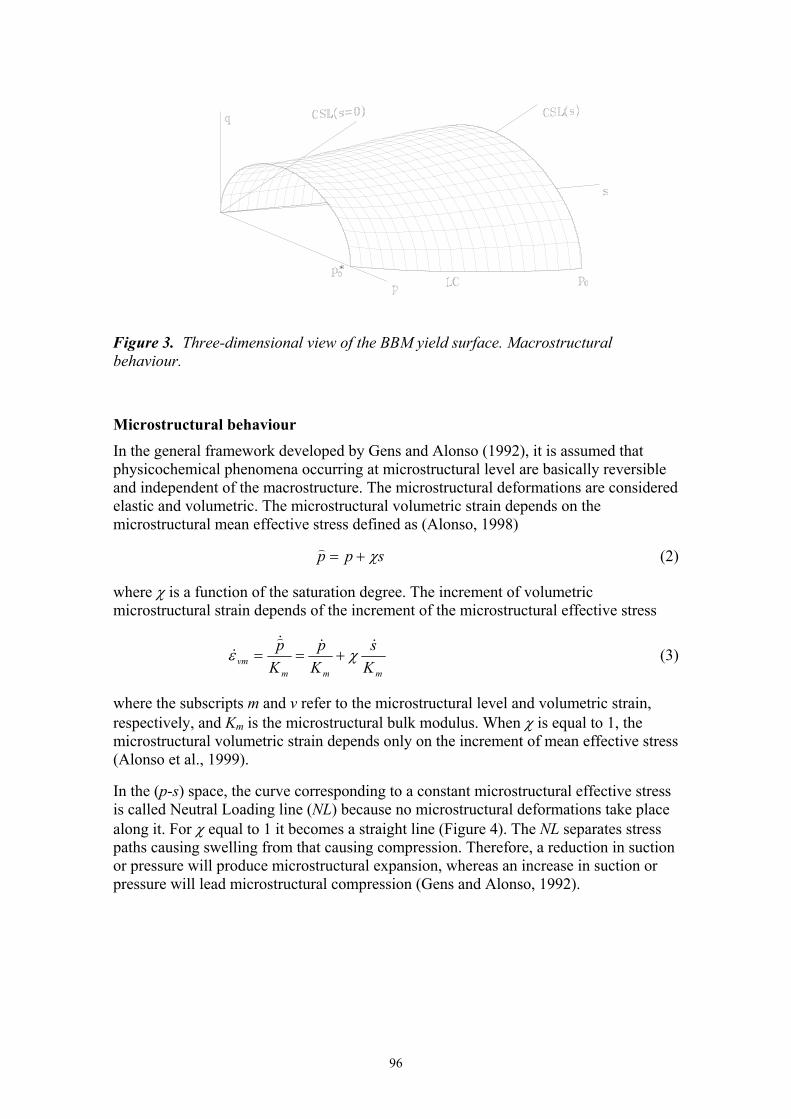
96

Figure 3. Three-dimensional view of the BBM yield surface. Macrostructural behaviour.

Microstructural behaviour In the general framework developed by Gens and Alonso (1992), it is assumed that physicochemical phenomena occurring at microstructural level are basically reversible and independent of the macrostructure. The microstructural deformations are considered elastic and volumetric. The microstructural volumetric strain depends on the microstructural mean effective stress defined as (Alonso, 1998)

spp χ+= (2)

where χ is a function of the saturation degree. The increment of volumetric microstructural strain depends of the increment of the microstructural effective stress

mmmvm K

sKp

Kp χε +== (3)

where the subscripts m and v refer to the microstructural level and volumetric strain, respectively, and Km is the microstructural bulk modulus. When χ is equal to 1, the microstructural volumetric strain depends only on the increment of mean effective stress (Alonso et al., 1999).

In the (p-s) space, the curve corresponding to a constant microstructural effective stress is called Neutral Loading line (NL) because no microstructural deformations take place along it. For χ equal to 1 it becomes a straight line (Figure 4). The NL separates stress paths causing swelling from that causing compression. Therefore, a reduction in suction or pressure will produce microstructural expansion, whereas an increase in suction or pressure will lead microstructural compression (Gens and Alonso, 1992).

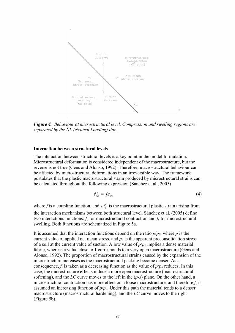
97

Figure 4. Behaviour at microstructural level. Compression and swelling regions are separated by the NL (Neutral Loading) line.

Interaction between structural levels The interaction between structural levels is a key point in the model formulation. Microstructural deformation is considered independent of the macrostructure, but the reverse is not true (Gens and Alonso, 1992). Therefore, macrostructural behaviour can be affected by microstructural deformations in an irreversible way. The framework postulates that the plastic macrostructural strain produced by microstructural strains can be calculated throughout the following expression (Sánchez et al., 2005)

vmp

v fεε β = (4)

where f is a coupling function, and pvβε is the macrostructural plastic strain arising from

the interaction mechanisms between both structural level. Sánchez et al. (2005) define two interactions functions: fc for microstructural contraction and fs for microstructural swelling. Both functions are schematized in Figure 5a.

It is assumed that the interaction functions depend on the ratio p/p0, where p is the current value of applied net mean stress, and p0 is the apparent preconsolidation stress of a soil at the current value of suction. A low value of p/p0 implies a dense material fabric, whereas a value close to 1 corresponds to a very open macrostructure (Gens and Alonso, 1992). The proportion of macrostructural strains caused by the expansion of the microstructure increases as the macrostructural packing become denser. As a consequence, fs is taken as a decreasing function as the value of p/p0 reduces. In this case, the microstructure effects induce a more open macrostructure (macrostructural softening), and the LC curve moves to the left in the (p-s) plane. On the other hand, a microstructural contraction has more effect on a loose macrostructure, and therefore fc is assumed an increasing function of p/p0. Under this path the material tends to a denser macrostructure (macrostructural hardening), and the LC curve moves to the right (Figure 5b).

98

ε / εβ

Figure 5. Micro and macrostructural coupling. (a) Interaction functions. (b) Movements of the LC curve due to microstructural effects.

The coupling between both mechanisms is considered assuming that (Sánchez et al., 2005)

pv

pvLC

pv βεεε += (5)

where pvε is the total volumetric plastic strain, and p

vLCε is the plastic volumetric strain induced by the BBM (macrostructural behaviour).

A detailed description of the whole model is presented in Sánchez et al. (2005). It was implemented in the finite element program CODE_BRIGHT (Olivella et al., 1996).

4.2 Test simulation TBT_3 mock-up experiment was previously simulated by UPC group using BBM (Ledesma et al., 2006). However, calculated stress results shown important differences with experimental results. Because of that, it was decided to use the BExM in order improve the stress predictions.

Some small modification in the retention curve (Sm and m values) respect to that used in the previous simulation (using the BBM) has been done. The following parameters are adopted in this case

0P (MPa) = 30.0 β = 0.3 mS (MPa) = 1000 m = 2.0

The parameters defining the mechanical behaviour are indicated in Table 1. The microstructural behaviour is defined by the following law (Alonso, 1998)

m

p

m

meKβ

α ˆ−

= (6)

where αm and βm are material parameters. The adopted interaction functions are similar to that presented in Sánchez et al. (2005). The initial void ratio is 0.46 and 0.20 for micro and macrostructural levels, respectively.

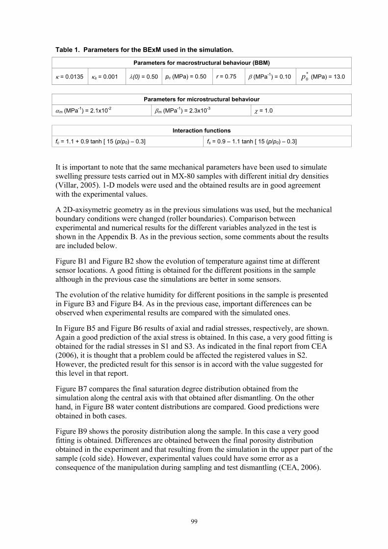
99

Table 1. Parameters for the BExM used in the simulation.

Parameters for macrostructural behaviour (BBM)

κ = 0.0135 κs = 0.001 λ(0) = 0.50 pc (MPa) = 0.50 r = 0.75 β (MPa-1) = 0.10 *0p (MPa) = 13.0

Parameters for microstructural behaviour

αm (MPa-1) = 2.1x10-2 βm (MPa-1) = 2.3x10-3 χ = 1.0

Interaction functions

fc = 1.1 + 0.9 tanh [ 15 (p/p0) – 0.3] fs = 0.9 – 1.1 tanh [ 15 (p/p0) – 0.3]

It is important to note that the same mechanical parameters have been used to simulate swelling pressure tests carried out in MX-80 samples with different initial dry densities (Villar, 2005). 1-D models were used and the obtained results are in good agreement with the experimental values.

A 2D-axisymetric geometry as in the previous simulations was used, but the mechanical boundary conditions were changed (roller boundaries). Comparison between experimental and numerical results for the different variables analyzed in the test is shown in the Appendix B. As in the previous section, some comments about the results are included below.

Figure B1 and Figure B2 show the evolution of temperature against time at different sensor locations. A good fitting is obtained for the different positions in the sample although in the previous case the simulations are better in some sensors.

The evolution of the relative humidity for different positions in the sample is presented in Figure B3 and Figure B4. As in the previous case, important differences can be observed when experimental results are compared with the simulated ones.

In Figure B5 and Figure B6 results of axial and radial stresses, respectively, are shown. Again a good prediction of the axial stress is obtained. In this case, a very good fitting is obtained for the radial stresses in S1 and S3. As indicated in the final report from CEA (2006), it is thought that a problem could be affected the registered values in S2. However, the predicted result for this sensor is in accord with the value suggested for this level in that report.

Figure B7 compares the final saturation degree distribution obtained from the simulation along the central axis with that obtained after dismantling. On the other hand, in Figure B8 water content distributions are compared. Good predictions were obtained in both cases.

Figure B9 shows the porosity distribution along the sample. In this case a very good fitting is obtained. Differences are obtained between the final porosity distribution obtained in the experiment and that resulting from the simulation in the upper part of the sample (cold side). However, experimental values could have some error as a consequence of the manipulation during sampling and test dismantling (CEA, 2006).

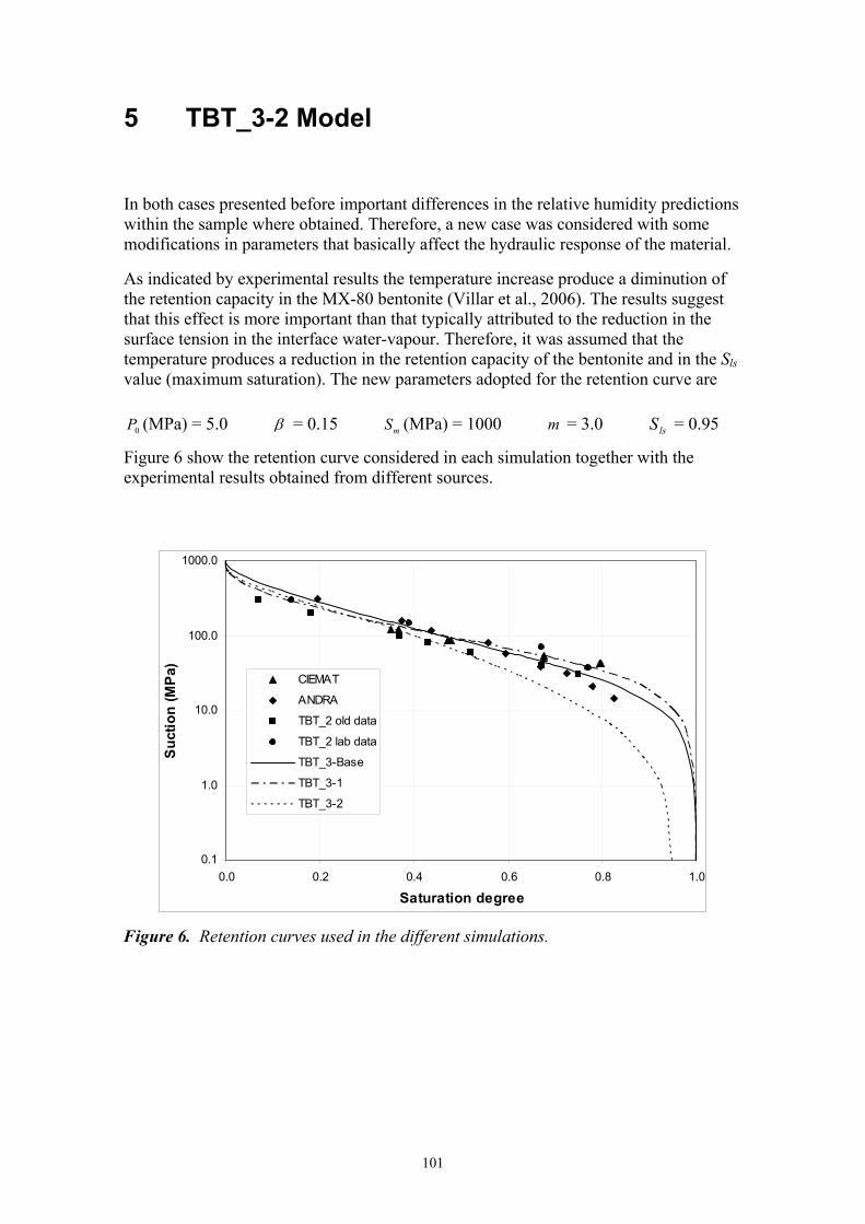
101

5 TBT_3-2 Model

In both cases presented before important differences in the relative humidity predictions within the sample where obtained. Therefore, a new case was considered with some modifications in parameters that basically affect the hydraulic response of the material.

As indicated by experimental results the temperature increase produce a diminution of the retention capacity in the MX-80 bentonite (Villar et al., 2006). The results suggest that this effect is more important than that typically attributed to the reduction in the surface tension in the interface water-vapour. Therefore, it was assumed that the temperature produces a reduction in the retention capacity of the bentonite and in the Sls value (maximum saturation). The new parameters adopted for the retention curve are

0P (MPa) = 5.0 β = 0.15 mS (MPa) = 1000 m = 3.0 lsS = 0.95

Figure 6 show the retention curve considered in each simulation together with the experimental results obtained from different sources.

0.1

1.0

10.0

100.0

1000.0

0.0 0.2 0.4 0.6 0.8 1.0

Saturation degree

Suc

tion

(MPa

)

CIEMAT

ANDRA

TBT_2 old data

TBT_2 lab data

TBT_3-Base

TBT_3-1

TBT_3-2

Figure 6. Retention curves used in the different simulations.

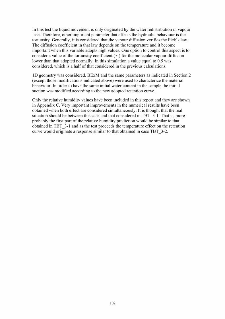
102

In this test the liquid movement is only originated by the water redistribution in vapour fase. Therefore, other important parameter that affects the hydraulic behaviour is the tortuosity. Generally, it is considered that the vapour diffusion verifies the Fick’s law. The diffusion coefficient in that law depends on the temperature and it become important when this variable adopts high values. One option to control this aspect is to consider a value of the tortuosity coefficient (τ ) for the molecular vapour diffusion lower than that adopted normally. In this simulation a value equal to 0.5 was considered, which is a half of that considered in the previous calculations.

1D geometry was considered. BExM and the same parameters as indicated in Section 2 (except those modifications indicated above) were used to characterize the material behaviour. In order to have the same initial water content in the sample the initial suction was modified according to the new adopted retention curve.

Only the relative humidity values have been included in this report and they are shown in Appendix C. Very important improvements in the numerical results have been obtained when both effect are considered simultaneously. It is thought that the real situation should be between this case and that considered in TBT_3-1. That is, more probably the first part of the relative humidity prediction would be similar to that obtained in TBT_3-1 and as the test proceeds the temperature effect on the retention curve would originate a response similar to that obtained in case TBT_3-2.

103

6 Concluding Remarks

This report includes the results of the predictive modelling programme of the TBT_3 experiment performed by the group coordinated by ENRESA. The definition of the models and the parameters used in the computations follow the guidelines of the document by Clay Technology (2006) and CEA (2006).

The output of the simulation work has been presented in Section 3 and Appendix A, and includes time evolution of temperature, relative humidity and stresses (radial & axial). An additional case which keeps in fact all the thermal and hydraulic parameters, but changes the mechanical material model and the mechanical boundary condition has been presented in Section 4. The idea was to point out the importance of the mechanical model adopted to simulate the bentonite behaviour on the stress levels. A final simulation analyzes the influence of some parameters in the hydraulic response.

It is believed that the prediction of temperature variable is reasonably performed. In the case of relative humidity results it is necessary to modify some parameters in order to improve the obtained results (compare results for TBT_3-Base and TBT_3-1 with TBT_3-2). The prediction of mechanical variables (i.e. stresses) has been improved as a more adequate mechanical model has been adopted (TBT_3-1).

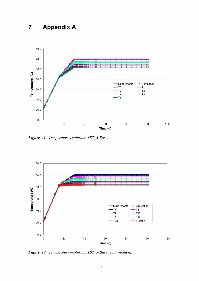
105

7 Appendix A

0.0

20.0

40.0

60.0

80.0

100.0

120.0

140.0

0 20 40 60 80 100 120

Time (d)

Tem

pera

ture

(ºC

)

Experimental SimulationT0 T1T2 T3T4 T5T6

Figure A1. Temperature evolution. TBT_3-Base.

0.0

20.0

40.0

60.0

80.0

100.0

120.0

0 20 40 60 80 100 120

Time (d)

Tem

pera

ture

(ºC

)

Experimental SimulationT7 T8T9 T10T11 T12T13 TPiston

Figure A2. Temperature evolution. TBT_3-Base (continuation).

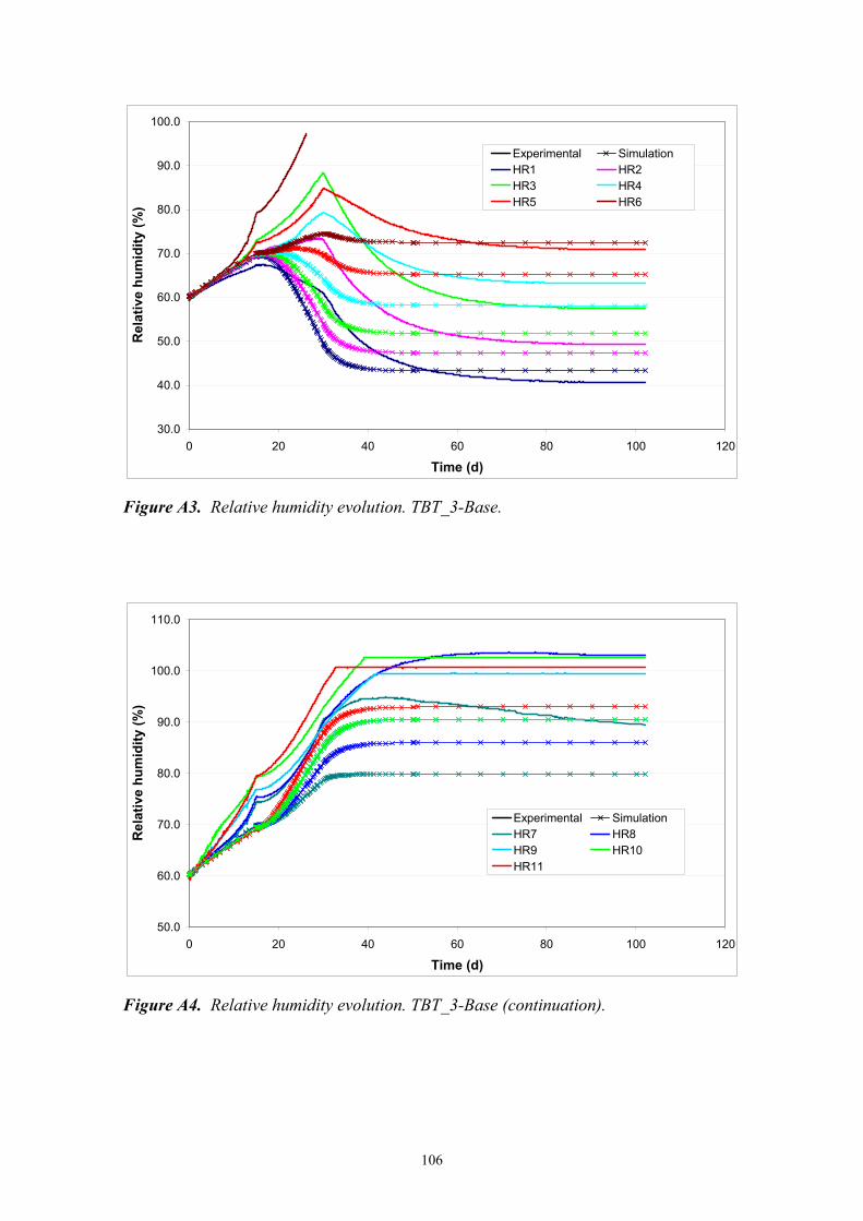
106

30.0

40.0

50.0

60.0

70.0

80.0

90.0

100.0

0 20 40 60 80 100 120

Time (d)

Rel

ativ

e hu

mid

ity (%

)Experimental SimulationHR1 HR2HR3 HR4HR5 HR6

Figure A3. Relative humidity evolution. TBT_3-Base.

50.0

60.0

70.0

80.0

90.0

100.0

110.0

0 20 40 60 80 100 120

Time (d)

Rel

ativ

e hu

mid

ity (%

)

Experimental SimulationHR7 HR8HR9 HR10HR11

Figure A4. Relative humidity evolution. TBT_3-Base (continuation).

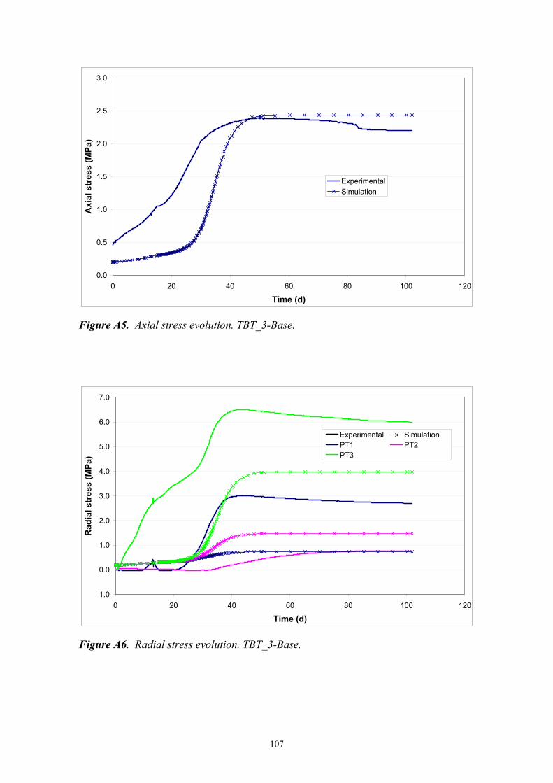
107

0.0

0.5

1.0

1.5

2.0

2.5

3.0

0 20 40 60 80 100 120

Time (d)

Axi

al s

tres

s (M

Pa)

ExperimentalSimulation

Figure A5. Axial stress evolution. TBT_3-Base.

-1.0

0.0

1.0

2.0

3.0

4.0

5.0

6.0

7.0

0 20 40 60 80 100 120

Time (d)

Rad

ial s

tres

s (M

Pa)

Experimental SimulationPT1 PT2PT3

Figure A6. Radial stress evolution. TBT_3-Base.

108

0.0

25.0

50.0

75.0

100.0

125.0

150.0

175.0

200.0

0.0 0.2 0.4 0.6 0.8 1.0

Saturation degree

Hig

h (m

m)


Figure A7. Saturation degree along the sample. TBT_3-Base.

0.0

25.0

50.0

75.0

100.0

125.0

150.0

175.0

200.0

0.0 5.0 10.0 15.0 20.0 25.0

Water content (%)

Hig

h (m

m)


Figure A8. Water content along the sample. TBT_3-Base.

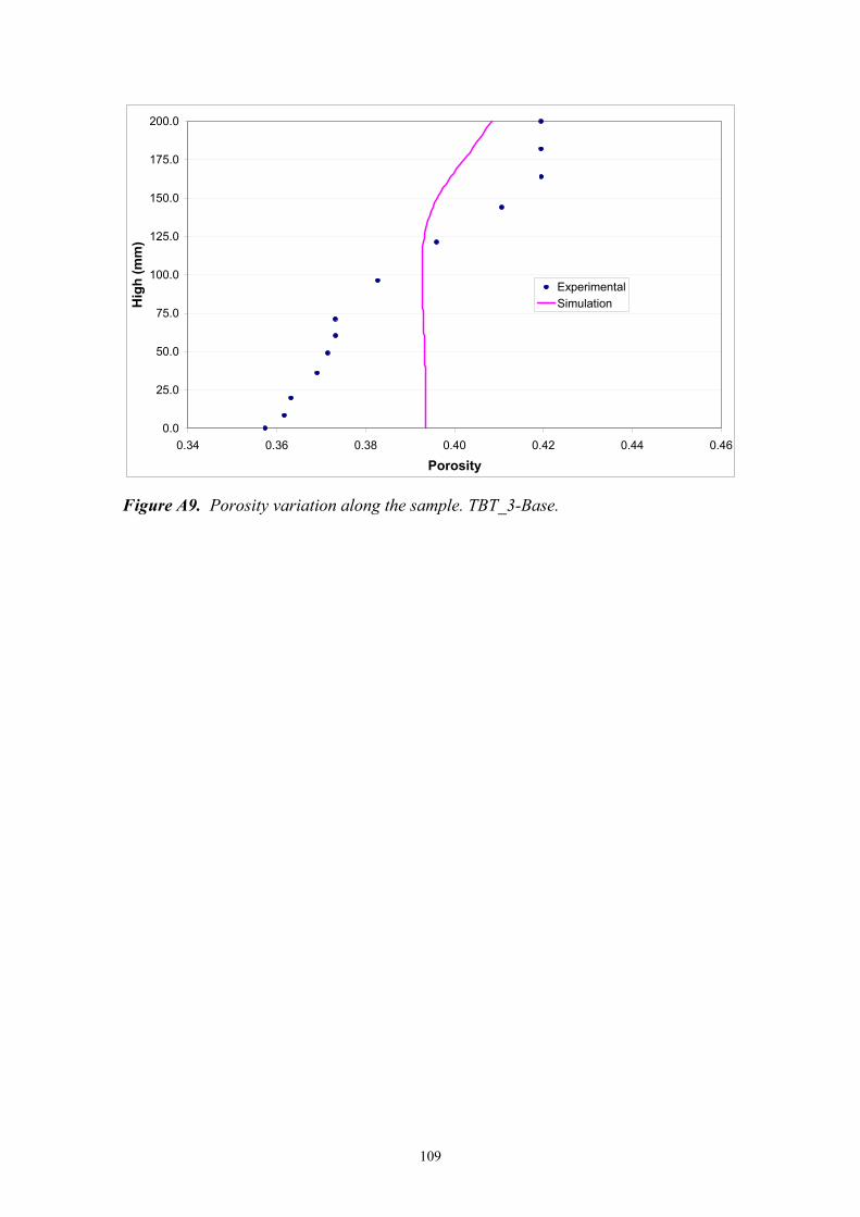
109

0.0

25.0

50.0

75.0

100.0

125.0

150.0

175.0

200.0

0.34 0.36 0.38 0.40 0.42 0.44 0.46

Porosity

Hig

h (m

m)


Figure A9. Porosity variation along the sample. TBT_3-Base.

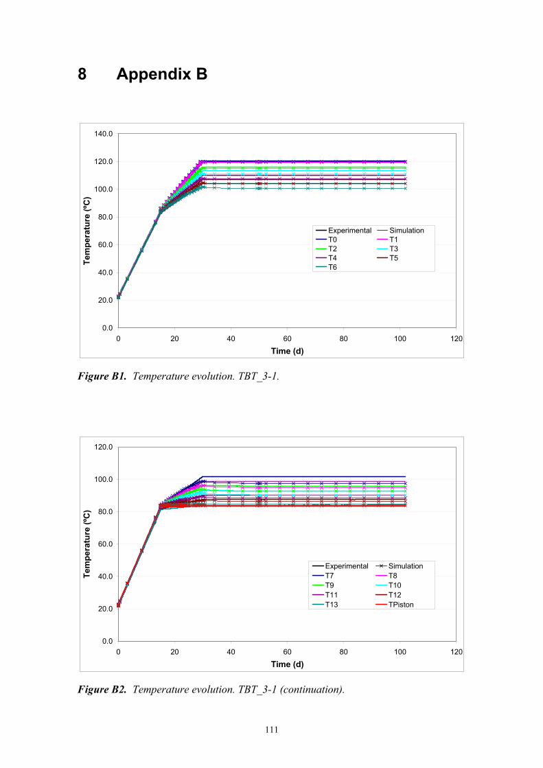
111

8 Appendix B

0.0

20.0

40.0

60.0

80.0

100.0

120.0

140.0

0 20 40 60 80 100 120

Time (d)

Tem

pera

ture

(ºC

)

Experimental SimulationT0 T1T2 T3T4 T5T6

Figure B1. Temperature evolution. TBT_3-1.

0.0

20.0

40.0

60.0

80.0

100.0

120.0

0 20 40 60 80 100 120

Time (d)

Tem

pera

ture

(ºC

)

Experimental SimulationT7 T8T9 T10T11 T12T13 TPiston

Figure B2. Temperature evolution. TBT_3-1 (continuation).

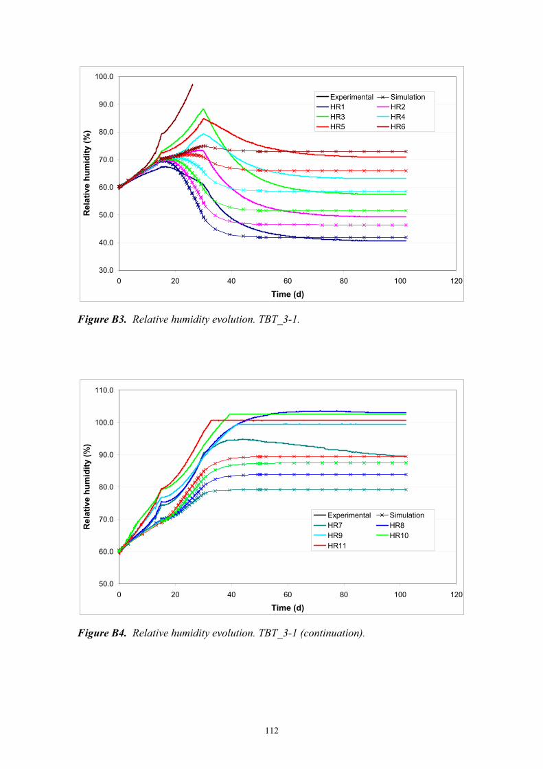
112

30.0

40.0

50.0

60.0

70.0

80.0

90.0

100.0

0 20 40 60 80 100 120

Time (d)

Rel

ativ

e hu

mid

ity (%

)Experimental SimulationHR1 HR2HR3 HR4HR5 HR6

Figure B3. Relative humidity evolution. TBT_3-1.

50.0

60.0

70.0

80.0

90.0

100.0

110.0

0 20 40 60 80 100 120

Time (d)

Rel

ativ

e hu

mid

ity (%

)

Experimental SimulationHR7 HR8HR9 HR10HR11

Figure B4. Relative humidity evolution. TBT_3-1 (continuation).

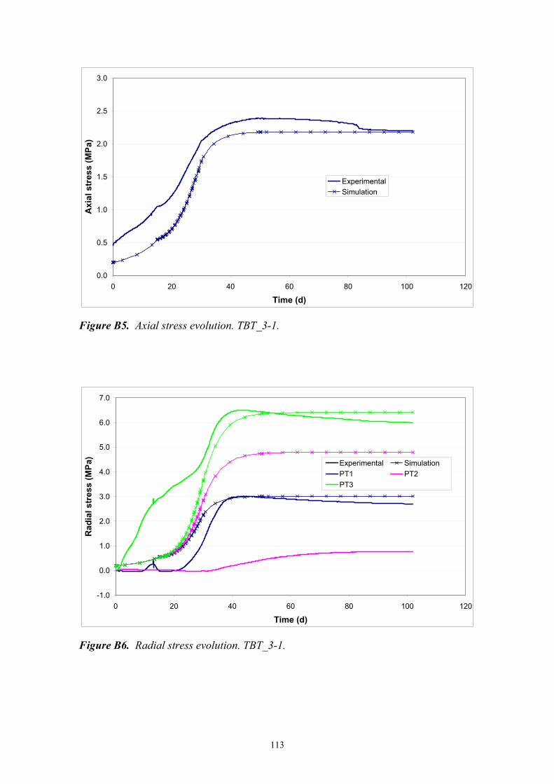
113

0.0

0.5

1.0

1.5

2.0

2.5

3.0

0 20 40 60 80 100 120

Time (d)

Axi

al s

tres

s (M

Pa)


Figure B5. Axial stress evolution. TBT_3-1.

-1.0

0.0

1.0

2.0

3.0

4.0

5.0

6.0

7.0

0 20 40 60 80 100 120

Time (d)

Rad

ial s

tres

s (M

Pa)

Experimental SimulationPT1 PT2PT3

Figure B6. Radial stress evolution. TBT_3-1.

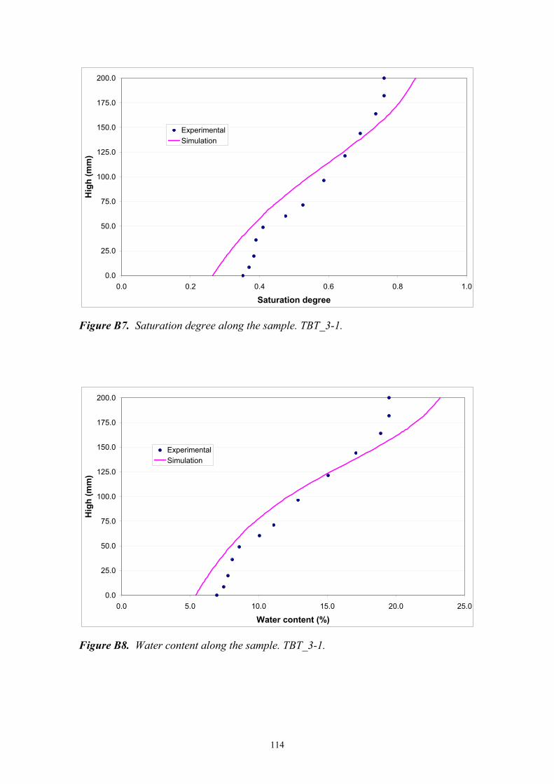
114

0.0

25.0

50.0

75.0

100.0

125.0

150.0

175.0

200.0

0.0 0.2 0.4 0.6 0.8 1.0

Saturation degree

Hig

h (m

m)


Figure B7. Saturation degree along the sample. TBT_3-1.

0.0

25.0

50.0

75.0

100.0

125.0

150.0

175.0

200.0

0.0 5.0 10.0 15.0 20.0 25.0

Water content (%)

Hig

h (m

m)


Figure B8. Water content along the sample. TBT_3-1.

115

0.0

25.0

50.0

75.0

100.0

125.0

150.0

175.0

200.0

0.34 0.36 0.38 0.40 0.42 0.44 0.46

Porosity

Hig

h (m

m)


Figure B9. Porosity distribution along the sample. TBT_3-1.

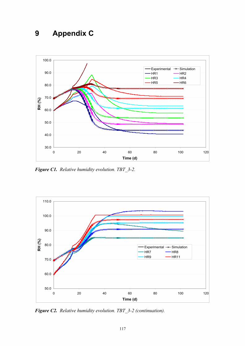
117

9 Appendix C

30.0

40.0

50.0

60.0

70.0

80.0

90.0

100.0

0 20 40 60 80 100 120

Time (d)

RH

(%)

Experimental SimulationHR1 HR2HR3 HR4HR5 HR6

Figure C1. Relative humidity evolution. TBT_3-2.

50.0

60.0

70.0

80.0

90.0

100.0

110.0

0 20 40 60 80 100 120

Time (d)

RH

(%)

Experimental SimulationHR7 HR8HR9 HR11

Figure C2. Relative humidity evolution. TBT_3-2 (continuation).

119

10 References

Alonso E., Vaunat J., Gens A. (1999). Modelling the mechanical behaviour of expansive clays. Engineering Geology, 54, 173-183.

Alonso E.E. (1998). Modelling expansive soil behaviour. Second International Conference on Unsaturated Soils. Beijing, China. Vol. 1, 37-70.

Alonso E.E., Gens A., Josa A. (1990). A constitutive model for partially saturated soils. Géotechnique, 40, 405-430.

Åkesson M., Hökmark H. (2006). TBT_3 – Predictive Modeling Program, March 2006. Clay Technology.

Gatabin C., Guillot W. (2006). TBT_3 Mock-up Tets. Final Report. July 2006. CEA.

Gens A., Alonso E.E. (1992). A framework for the behaviour of unsaturated expansive clays. Can. Geotech. J., 29, 1013-1032.

Ledesma A., Jacinto A., Velasco M. (2006). TBT_3 – Predictive Modelling Program. Simulation of TBT_3 Mockup Experiment. ENRESA Contibution. April, 2006.

Sánchez M., Gens A., Guimaraes L., Olivella S. (2005). A double structure generalized plasticity model for expansive materials. Int. J. Numer. Anal. Meth. Geomech., 29, 751–787.

Sánchez M. (2004). Coupled Thermo-Hydro-Mechanical analysis in low permeability media. Ph.D. Thesis, Geotechnical Engineering Department, Technical University of Catalunya, Spain.

Villar M.V., Gómez-Espina R., Martín P.L. (2006). Behaviour of MX-80 Bentonite at Unsaturated Conditions and under Thermo-Hydraulic Gradient. Informes Técnicos Ciemat. 1081. Julio, 2006.

Villar M.V. (2005). MX-80 Bentonite. Thermo-Hydro-Mechanical Characterisation Performed at CIEMAT in the Context of the Prototype Project. Informes Técnicos Ciemat. 1053. Febrero, 2005.

121

Appendix 5

Clay Technology AB


Lund, Sweden

TBT_3 Mock-up evaluation

May 2008

Mattias Åkesson

123

Contents

1 Background 125

2 Evaluation of experimental results 127 2.1 Vapor pressure and suction 127 2.2 In situ retention curve 129

3 Numerical modeling 131 3.1 Model description 131 3.2 Model results 133 3.3 Discussion of results 138

4 Concluding remarks 141

5 References 143

125

1 Background

Within the framework of the TBT evaluation modeling task force, it has been decided to emphasize the initial thermo-hydraulic condition around the lower heater in the TBT test. Of special interest are the phenomena of desaturation and the role of temperature gradients and temperature levels.


Due to an observed leak of heat in the midsection of the TBT_2 setup, an improved experimental design was developed for the follow-up TBT_3 test. This test also consisted of a combined experimental and blind predictive modeling work.

A description of the test and a guideline with requested modeling results was given in a modeling program /Åkesson and Hökmark, 2006/. The test was launched on March 9th 2006.

Blind predictions were presented at the modeling meeting at Äspö in April 2006 and were compared with the experimental results available at that time. Due to the novelty of the experimental results, the task was extended to include an evaluation modeling phase, in which the models were modified. This task was completed in November 2006. The experimental work and results have been reported /Gatabin and Guillot, 2006/.

This report describes the evaluation modeling of the Clay Tech modeling team. The work focused on the TH processes and included a detailed evaluation of experimental results as well as numerical modeling.

127

2 Evaluation of experimental results

2.1 Vapor pressure and suction From the results of temperature and relative humidity it is possible to calculate the development of vapor pressure and suction. These variables are calculated with a function for the saturation vapor pressure and Kelvin’s law in Code_Bright /CIMNE, 2002/:

)(136075),( 15.2737.5239

MPaeRHTRHp Tv

+−

⋅⋅= (1)

)()15.273()ln(),( PaM

TRRHTRHsw

w +⋅⋅⋅−=

ρ (2)

These two variables can be regarded as the moisture flow potentials of the system. In Code_Bright, the vapor mass fraction (ωg

w) is used instead of the vapor pressure, but these variables are directly related under conditions of constant gas pressure (pg):

wvairvg

wvwg MpMpp

Mp⋅+⋅−

⋅=

)(ϖ (3)

The development of the vapor pressure at the different sensor positions are shown in Figure 2-1. A clear separation can be noted for the period during which a thermal gradient were applied with vapor pressures ranging from 0.6 to 1.3 bar. The peak values above atmospheric pressure appear to correspond to the measured pore pressures (see Figure 2-4 in main report), which indicate that the cell was generally not gas tight, but allowed a minor pressure buildup at this point. The distribution of vapor pressure is further illustrated in Figure 2-2. Here it can be clearly seen than the vapor pressure at the hot end never exceeded 1 bar.

During the equilibration phase, the levels converged to a narrow range (Figure 2-1, right). The steady-state distribution shows lower values at the cold end which reflects the saturation vapor pressure for the temperatures at this part. In the central part of the specimen, between 50 and 150 mm height, the vapor pressures were found in a narrow interval between 0.79 and 0.82 bar. These values are based on tabulated saturation vapor pressures (Schmidt, 1982). Slightly lower vapor pressures were found at the hot end at steady-state.

Calculated suction values at the different sensor positions are shown in Figure 2-3. During the equilibration phase, the levels diverge to a quite wide range: from 0 to 160 MPa.

128

0

0,2

0,4

0,6

0,8

1

1,2

1,4

0 20 40 60 80 100 120

Time (days)

Vap

or p

ress

ure

(bar

)



0 50 100 150 2000

0.5

1

RH-sensorsT-sensors

Height (mm)

Vap

or p

ress

ure

(bar

)

Figure 2-1. Evaluated vapor pressure. Development with time, based on rh-sensor results and Eq 1 (left). Steady-state distributions, based on tabulated saturation vapor pressures (right): Temperatures from thermocouples (blue) and rh-sensors (red).

0

0,2

0,4

0,6

0,8

1

1,2

1,4

0 50 100 150 200Height (mm)

Vap

or p

ress

ure

(bar

) 015 days25 days30 days40 days102 days

Figure 2-2. Vapor pressure distributions at different times. Values based on temperatures from rh-sensors and Eq.1.

-200

20406080

100120140160180

0 20 40 60 80 100 120Time (days)

Suc

tion

(MP

a)



0 50 100 150 200

0

100

200RH-sensorsT-sensors

Height (mm)

Suct

ion

(MPa

)

Figure 2-3. Evaluated suction values. Development with time. Steady-state distributions prior to dismantling (right): Temperatures from thermocouples (blue) and rh-sensors (red).

129

The total moisture flux (j) can be described as the sum of the vapor flux and the liquid flux:

dxdpD

dxdpDj l

plv

pv −−= (4)

where Dpv and Dpl are the flow coefficients for the vapor and the liquid flow, respectively. This sum must be zero since steady-state conditions has been reached.

It should be noted that the vapor flow in this case is not only diffusive, but also convective, since the gas mixture can not be described as dilute. Nevertheless, it can be concluded from the low vapor pressure gradient and Eq.4 that the flow coefficient for the vapor flow must be much higher than for the liquid flow.

The opposite relation can be found at the cold end were the vapor was saturated and the liquid pressure gradient was very low. In this case the flow coefficient for the vapor flow must be much lower than for the liquid flow.

The steady-state distribution does not give any information of the absolute values of the flow coefficients, only their ratio. If the time to reach steady-state is considered, however, then this would reveal such information. This is further described in Section 3.

2.2 In situ retention curve Measured water contents and degrees of saturation enable an evaluation of an in situ retention curve together with the calculated suction values. Such relations are shown in Figure 2-4, both for steady-state conditions and after the 20 hour cooling period.

The relation between water contents and the post-cooling suction values are generally in accordance with retention data for free swelling samples, although suction data for HR9 and HR11 diverge to some extent.

The suction values for the steady-state conditions are on the other hand significantly lower than for free swelling samples. This is especially apparent when the retention data is presented for degrees of saturation. Under these experimental conditions the suction can apparently be zero, i.e. the vapor is saturated, even though the bentonite is not water saturated.

,

0 5 10 15 20 25 30 351

10

100

1 .103

Steady-stateAfter coolingClayTech data

Water content (%)

Suct

ion

(MPa

)

0.3 0.4 0.5 0.6 0.7 0.8 0.9 11

10

100

1 .103

Steady-stateAfter coolingModel


Suct

ion

(MPa

)

Figure 2-4. Retention curves: suction vs. water content (left) and suction vs. degree of saturation (right); at steady-state (red) and after cooling (blue). Black line in left graph is retention data for free swelling samples (interpolated data from /Dueck,2004/. Dashed line in right graph is a van-Genuchten relation used in this work.

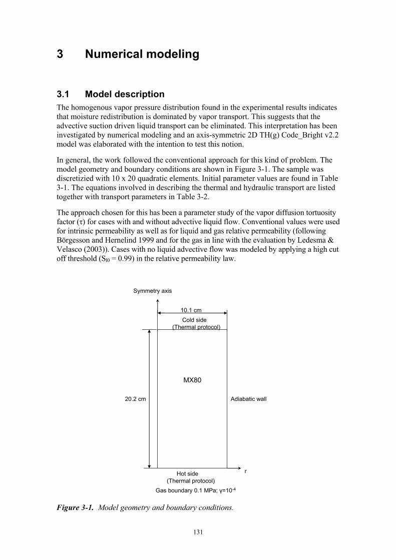
131

3 Numerical modeling

3.1 Model description The homogenous vapor pressure distribution found in the experimental results indicates that moisture redistribution is dominated by vapor transport. This suggests that the advective suction driven liquid transport can be eliminated. This interpretation has been investigated by numerical modeling and an axis-symmetric 2D TH(g) Code_Bright v2.2 model was elaborated with the intention to test this notion.

In general, the work followed the conventional approach for this kind of problem. The model geometry and boundary conditions are shown in Figure 3-1. The sample was discretizied with 10 x 20 quadratic elements. Initial parameter values are found in Table 3-1. The equations involved in describing the thermal and hydraulic transport are listed together with transport parameters in Table 3-2.

The approach chosen for this has been a parameter study of the vapor diffusion tortuosity factor (τ) for cases with and without advective liquid flow. Conventional values were used for intrinsic permeability as well as for liquid and gas relative permeability (following Börgesson and Hernelind 1999 and for the gas in line with the evaluation by Ledesma & Velasco (2003)). Cases with no liquid advective flow was modeled by applying a high cut off threshold (Sl0 = 0.99) in the relative permeability law.

10.1 cm

20.2 cm

Symmetry axis

r

Gas boundary 0.1 MPa; γ=10-4


Adiabatic wall

MX80


Figure 3-1. Model geometry and boundary conditions.

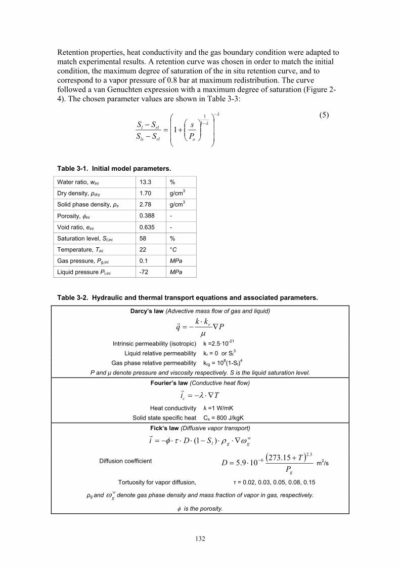
132

Retention properties, heat conductivity and the gas boundary condition were adapted to match experimental results. A retention curve was chosen in order to match the initial condition, the maximum degree of saturation of the in situ retention curve, and to correspond to a vapor pressure of 0.8 bar at maximum redistribution. The curve followed a van Genuchten expression with a maximum degree of saturation (Figure 2-4). The chosen parameter values are shown in Table 3-3:

λ

λ

−

−

⎟⎟⎟

⎠

⎞

⎜⎜⎜

⎝

⎛

⎟⎟⎠

⎞⎜⎜⎝

⎛+=

−− 1

1

1orlls

rll

Ps

SSSS

(5)

Table 3-1. Initial model parameters.

Water ratio, wini 13.3 %

Dry density, ρdry 1.70 g/cm3

Solid phase density, ρs 2.78 g/cm3

Porosity, φini 0.388 -

Void ratio, eini 0.635 -

Saturation level, Sl,ini 58 %

Temperature, Tini 22 °C

Gas pressure, Pg,ini 0.1 MPa

Liquid pressure Pl,ini -72 MPa

Table 3-2. Hydraulic and thermal transport equations and associated parameters.

Darcy’s law (Advective mass flow of gas and liquid)

Pkk

q r ∇⋅

−=μ

Intrinsic permeability (isotropic) k =2.5·10-21 Liquid relative permeability kr = 0 or Sl

3 Gas phase relative permeability krg = 108(1-Sl)4

P and μ denote pressure and viscosity respectively. S is the liquid saturation level.

Fourier’s law (Conductive heat flow)

Tic ∇⋅−= λ

Heat conductivity λ =1 W/mK Solid state specific heat Cs = 800 J/kgK

Fick’s law (Diffusive vapor transport) wgglSDi ωρτφ ∇⋅⋅−⋅⋅⋅−= )1(

Diffusion coefficient ( )

gPTD

3.26 15.273109.5 +

⋅= − m2/s

Tortuosity for vapor diffusion, τ = 0.02, 0.03, 0.05, 0.08, 0.15

ρg and wgω denote gas phase density and mass fraction of vapor in gas, respectively.

φ is the porosity.

133

Table 3-3. Retention curve parameters.

P0 λ Srl Sls

77.39 MPa 0.45 0 0.77

Table 3-4. Thermal protocol.

Day Hot side temperature Cold side temperature

0 - 15 22 → 84 ºC 22 → 84 ºC

15 - 30 84 → 120 ºC 84 ºC

30 - 102 120 ºC 84 ºC

A constant thermal conductivity was chosen in order to capture the linear temperature distribution found in the experiment. A value of 1 W/mK was chosen. This is a typical value for MX-80 with a saturation degree of 58 % (Börgesson et al. 1995). Finally, a gas boundary with atmospheric pressure and a low transfer coefficient (γ = 10-4) was applied in order to capture the results of the pore pressure sensors.

3.2 Model results The steady-state moisture distribution and the time to reach this state were analyzed for different τ values, and for cases with and without advective liquid flow. The results are shown in Figure 3-2. It was confirmed that the models without advective liquid flow in all case reached the maximum redistribution and that the time needed to reach this state could be set for a certain τ value. It was found that a value of 0.03 gave good agreement with experimental data in these respects.

For the models with advective flow, both the steady-state distribution and the time were dependent on the τ value. And in order to reach the maximum redistribution, a higher τ value (0.15) had to be chosen. With this value, the time to reach steady-state was significantly shorter than was found in the experiment.

0,3

0,4

0,5

0,6

0,7

0,8

0 20 40 60 80 100

Time (days)

Deg

ree

of s

atur

atio

n (-

)

Tau = 0.02

Tau = 0.03

Tau = 0.05

Tau = 0.08

Tau = 0.15

0,3

0,4

0,5

0,6

0,7

0,8

0 20 40 60 80 100Time (days)

Deg

ree

of s

atur

atio

n (-

)

Tau = 0.02

Tau = 0.03

Tau = 0.05

Tau = 0.08

Tau = 0.15

Figure 3-2. Moisture redistribution for different vapor diffusion tortuosity values, illustrated as degrees of saturation at the hot and the cold end. Models without advective flow (left) and with advective flow (right).

134

0

20

40

60

80

100

120

140

0 20 40 60 80 100 120

Time (days)

Tem

pera

ture

(C)

T0 T1 T2 T3 T4 T5 T6T7 T8 T9 T10 T11 T12 T13 T0 T1 T2 T3 T4 T5 T6 T7 T8 T9 T10 T11 T12 T13

Figure 3-3. Temperature. Development with time: model without advective flow and τ = 0.03(dots) and experimental results (lines).

0

20

40

60

80

100

120

140

0 20 40 60 80 100 120

Time (days)

Tem

pera

ture

(C)

T0 T1 T2 T3 T4 T5 T6T7 T8 T9 T10 T11 T12 T13 T0 T1 T2 T3 T4 T5 T6 T7 T8 T9 T10 T11 T12 T13

Figure 3-4. Temperature. Development with time: model with advective flow and τ = 0.15 (dots) and experimental results (lines).

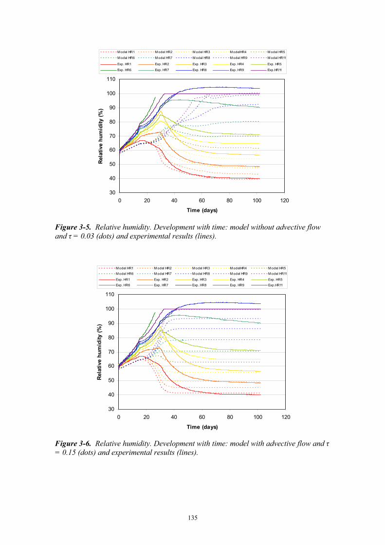
135

30

40

50

60

70

80

90

100

110

0 20 40 60 80 100 120

Time (days)

Rela

tive

hum

idity

(%)

M odel HR1 M odel HR2 M odel HR3 M odelHR4 M odel HR5

M odel HR6 M odel HR7 M odel HR8 M odel HR9 M odel HR11

Exp. HR1 Exp. HR2 Exp. HR3 Exp. HR4 Exp. HR5

Exp. HR6 Exp. HR7 Exp. HR8 Exp. HR9 Exp.HR11

Figure 3-5. Relative humidity. Development with time: model without advective flow and τ = 0.03 (dots) and experimental results (lines).

30

40

50

60

70

80

90

100

110

0 20 40 60 80 100 120

Time (days)

Rela

tive

hum

idity

(%)

M odel HR1 M odel HR2 M odel HR3 M odelHR4 M odel HR5M odel HR6 M odel HR7 M odel HR8 M odel HR9 M odel HR11

Exp. HR1 Exp. HR2 Exp. HR3 Exp. HR4 Exp. HR5Exp. HR6 Exp. HR7 Exp. HR8 Exp. HR9 Exp.HR11

Figure 3-6. Relative humidity. Development with time: model with advective flow and τ = 0.15 (dots) and experimental results (lines).

136

Results from both these models are compared with experimental results in Figures 3-3 to 3-10. The thermal development is shown in Figure 3-3 and 3-4, and in both cases it can be seen that the model results follows the experimental results. The evolution of model relative humidity at the sensor positions is shown together with experimental results in Figure 3-5 and 3-6. The separation of the rh-levels and the time-scale for this are reasonably well captured by the model without advection (Figure 3-5), especially at the hot end and during the final phase. During the second phase, however, when the thermal gradient was increased, and especially at the cold end, the agreement was less good.

The steady-state distributions of relative humidity and degree of saturation are shown in Figure 3-7 and 3-8, respectively. The model and the experimental saturation distributions are in good agreement, whereas the model rh distribution is slightly lower than the experimental results.

The evolution of gas pressure at the positions of the pore pressure sensors is shown in Figure 3-9. These results can be compared with experimental data in Figure 2-4 in the main report. It can be noticed that the model without advection displays a fairly homogenous gas pressure, whereas the gas pressure in the model with advection flow decreases towards the cold end.

Finally, the final vapor pressure distributions and the evolution of gas pressure are shown in Figure 3-10. The experimental results (based on tabulated saturation vapor pressures and thermocouple temperatures readings) are shown together model distributions; both with and without advective flow. Whereas the model without advection follows the experimental data quite good, the model with advective flow still deviates to some extent.

0

20

40

60

80

100

120

0 50 100 150 200

Height (mm)

Rel

ativ

e hu

mid

ity (%

)

Model

Experiment

0

20

40

60

80

100

120

0 50 100 150 200

Height (mm)

Rel

ativ

e hu

mid

ity (%

)

Model

Experiment

Figure 3-7. Stead-state distribution of relative humidity. Model without advective flow and τ = 0.03 (left); model with advective flow and τ = 0.15 (right).

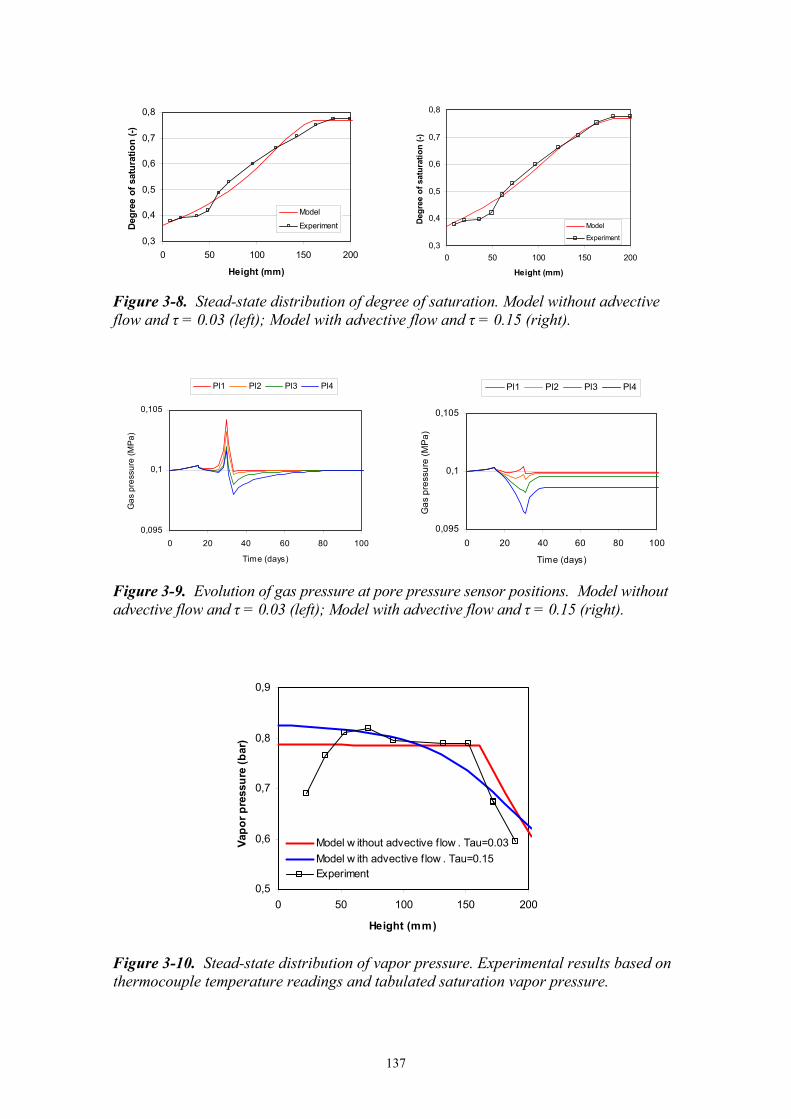
137

0,3

0,4

0,5

0,6

0,7

0,8

0 50 100 150 200

Height (mm)

Deg

ree

of s

atur

atio

n (-)

Model

Experiment

0,3

0,4

0,5

0,6

0,7

0,8

0 50 100 150 200

Height (mm)

Degr

ee o

f sat

urat

ion

(-)

Model

Experiment

Figure 3-8. Stead-state distribution of degree of saturation. Model without advective flow and τ = 0.03 (left); Model with advective flow and τ = 0.15 (right).

0,095

0,1

0,105

0 20 40 60 80 100

Time (days)

Gas

pre

ssur

e (M

Pa)

Pl1 Pl2 Pl3 Pl4

0,095

0,1

0,105

0 20 40 60 80 100

Time (days)

Gas

pre

ssur

e (M

Pa)

Pl1 Pl2 Pl3 Pl4

Figure 3-9. Evolution of gas pressure at pore pressure sensor positions. Model without advective flow and τ = 0.03 (left); Model with advective flow and τ = 0.15 (right).

0,5

0,6

0,7

0,8

0,9

0 50 100 150 200

Height (mm)

Vapo

r pre

ssur

e (b

ar)

Model w ithout advective f low . Tau=0.03Model w ith advective f low . Tau=0.15Experiment

Figure 3-10. Stead-state distribution of vapor pressure. Experimental results based on thermocouple temperature readings and tabulated saturation vapor pressure.

138

3.3 Discussion of results The TBT_3 mock-up test displayed a number of novel characteristics. Further investigations are however needed in order to confirm, explain and describe these phenomena thoroughly. The following interpretations can at present be drawn from the available experimental results.

The steady-state condition exhibited a homogenous vapor pressure profile. This observation suggests, together with the argument concerning the time-scale to reach steady-state, that the vapor pressure is the dominating potential for moisture transport in the investigated experiment. A conceptual explanation for the apparent lack of liquid transfer can tentatively be sought in terms of liquid continuity. The unsaturated hydraulic conductivity has earlier been proposed to diminish when the moisture content is lower than a certain value, below which the liquid continuity is broken (Philip and de Vries, 1957). Moreover, a concentration of the temperature gradient over the gas phase, as was a part of the Philip and de Vries-theory, would imply a low suction gradient over the hydrated particles, even though the vapor pressure is homogenous.

The analysis of the transport coefficients showed that the tortuosity factor had to be assigned a very low value (< 0.1) in order to capture the time scale to reach steady-state. This value underestimated, on the other hand, the rate of transfer at the cold end. The current formulation of the function for the vapor diffusion coefficient in Code_Bright (which is proportional to 1-Sl) may therefore have to be modified. For unsaturated isothermal conditions the flow potential can in principal be chosen freely, for instance as the water content or the liquid pressure. If a flow coefficient, Dpl(Sl), can be found that describes the hydration process in terms of gradients in liquid pressure, then the same results can be obtained in terms of gradients in vapor pressure for the flow coefficient Dpv = dpl/dpv·Dpl(Sl). The power law factor Sl

3, possibly with a step function at the point of vapor saturation, therefore appears to be an appropriate first choice of investigation. Such a function would explain the observed relatively low rate of vapor pressure reduction at the hot end in the experiment, in which the water content reduced from 13 to 7 %. The possibility that this slow response reflects the rate of dehydration, i.e. the transition from water to vapor, and not only the rate of vapor transfer, should however not be excluded.

The evaluated in situ retention curve implies that the suction value can be zero, i.e. the vapor is saturated, even though the bentonite is not water saturated. This was also applied in the modeling work through the specification of a maximum saturation degree (Sls in Eq. 5). Retention curves with such limits are however not generally applicable. For instance, if the specimen would have been exposed to a high water pressure at the cold end, then total saturation would occur at this location. The apparent retention curve is consequently not strictly decreasing and exhibits constant zero suction in a certain saturation interval. However, since the liquid pressure is used as a state variable, it appears to be necessary to adopt a strictly decreasing function. Such an adoption should, of course, follow the empirical relation as closely as possible.

139

An explanation for the evaluated retention properties can be sought in terms of pressure and temperature dependence. The pressure dependence of the retention properties has earlier been described as the difference between unloaded suction value and the load term αP, where α is the compressibility factor and P is the actual load (e.g. Dueck, 2004; Kassiff and Ben Shalom (1971). The value of α should be close to unity at saturated conditions. Kassiff and Ben Shalom (1971) found however values far greater than one at water contents around 20 %. Moreover, the notion of grain to grain contact stresses that exceed the measurable total stress has been proposed and elaborated by Åkesson and Hökmark (2007). In addition, experimental results by Villar and Gómez-Espina (2007) show that the suction value decreases with increasing temperatures. This would imply that the real suction relation for a given water content is composed of three terms: one representing the unloaded retention curve at reference temperature, one representing the influence of pressure and finally one term for the temperature dependence.

141

4 Concluding remarks

The TBT_3 experiment demonstrates two novel results: (1) a homogenous vapor pressure profile at steady-state; and (2) an in situ retention curve which implies that the buffer material can be in equilibrium with saturated vapor, even though the bentonite is not water saturated.

The first observation implies that the vapor pressure is the dominating potential for moisture transport (at least in cases with the studied water content, density and thermal conditions studied here) i.e.the ratio between the transport coefficients describing vapor diffusion and advective liquid flow would be significantly higher than is usually assumed.

In the presented models the advective flow had to be eliminated, in order to get a good agreement with the steady-state moisture distribution and the time to reach this condition. The model with the best agreement still showed some inconsistencies, especially regarding the evolution of relative humidity at the cold end. This could possibly be improved by modification of the function for the diffusion coefficient and the description of the retention properties.

143

5 References

Börgesson L., Johannesson L-E, Sandén T. and Hernelind J., 1995. Modeling of the physical behavior of water saturated clay barriers. Laboratory tests, material models and finite element application. SKB Technical Report TR-95-20.

Börgesson L., Hernelind J., 1999. Coupled thermo-hydro-mechanical calculations of the water saturation phase of a KBS-3 deposition hole. SKB Technical Report TR-99-41.

CIMNE, 2002. CODE_BRIGHT. A 3-D program for thermo-hydro-mechanical analysis in geological media. Departamento de Ingeneria del Terreno; Cartgrafica y Geofisica, UPC, Barcelona, Spain.

Dueck A. 2004. Hydro-mechanical properties of a water unsaturated sodium bentonite. Laboratory study and theoretical interpretation. Division of Soil Mechanics and Foundation Engineering, Lund Institute of Technology, Lund, Sweden.

Gatabin C., Guillot W. 2006. TBT_3 Mock-up test, Final report, July 2006. NT DPC/SCCME 06-345-A

Kassiff G., Ben Shalom A. 1971. Experimental relationship between swell pressure and suction. Géotechnique 21, 245-255.

Ledesma A., Velasco. M. 2003. Temperature Buffer Test. Predictive Modeling Performed by ENRESA.

Philip J.R., de Vries D.A. 1957. Moisture movement in porous materials under temperature gradients. Trans., Am. Geophys. Union., 38, 222-232.

Schmidt, E. 1982. Properties of Water and Steam in SI-Units. Springer-Verlag. Berlin.

Villar M.V., Gómez-Espina R. 2007. Retention curves of two bentonites at high temperature. In: Springer Proceedings in Physics 112: 267-274.

Åkesson M., Hökmark H. 2006. TBT_3 – Predictive modeling program. Clay Technology AB, Lund.

Åkesson M., Hökmark H. 2007. Mechanical Model for Unsaturated MX-80. In: Springer Proceedings in Physics 113: 3-10.

Äspö hard rock laboratory - skb · tbt (temperature buffer test) is a joint project between...

Documents