Svensk Kärnbränslehantering ABSwedish Nuclear Fueland Waste Management Co

Box 250, SE-101 24 Stockholm Phone +46 8 459 84 00

P-13-47

Äspö Task Force on modelling of groundwater flow and transport of solutes

Hierarchical modelling of groundwater flow at Okiluoto site by KAERI: Uncertainty and lessons

Nak-Youl Ko, Sung-Hoon Ji Korea Atomic Energy Research Institute (KAERI)

January 2017

Tänd ett lager: P, R eller TR.

Äspö Task Force on modelling of groundwater flow and transport of solutes

Hierarchical modelling of groundwater flow at Okiluoto site by KAERI: Uncertainty and lessons

Nak-Youl Ko, Sung-Hoon Ji Korea Atomic Energy Research Institute (KAERI)

ISSN 1651-4416SKB P-13-47ID 1413482

January 2017

This report concerns a study which was conducted for Svensk Kärnbränslehantering AB (SKB). The conclusions and viewpoints presented in the report are those of the authors. SKB may draw modified conclusions, based on additional literature sources and/or expert opinions.

Data in SKB’s database can be changed for different reasons. Minor changes in SKB’s database will not necessarily result in a revised report. Data revisions may also be presented as supplements, available at www.skb.se.

A pdf version of this document can be downloaded from www.skb.se.

© 2017 Svensk Kärnbränslehantering AB

SKB P-13-47 3

Abstract

To provide a bridge between the site characterisation and performance assessment approaches to pumping tests, we conducted simulations for modelling the groundwater flow system in the Olkiluoto island, Finland, with a stepwise approach at different modelling scales. Firstly, a regional-scale ground-water flow model including the entire area of the Olkiluoto island was constructed so as to simulate a hydraulic test, with pumping at the KR24 borehole. Secondly, a block scale groundwater flow domain located at the central part of the Olkiluoto island was modelled for simulating pumping tests performed at the KR14 and KR18 boreholes. Finally, groundwater flow in a single fracture, identified at the depth of about 250 m below ground surface and observed in the boreholes drilled from the under ground research tunnel was considered.

In the regional-scale simulation, it was revealed that open deep boreholes are likely to influence groundwater flow systems in low-permeable rock media by increasing vertical hydraulic conductivity.

In the block-scale simulation, the simulation using the open borehole condition may not show the natural groundwater flow system, as the open boreholes could be new conduits and have the same effect as fractures on the groundwater flow. The simulated values of the flow rates in the boreholes became similar to the measurements from the study field, especially those of local groundwater flows. It showed that considering background fractures can decrease uncertainty in the results of the groundwater flow simulations by representing such small variations in the model domain.

In the single fracture simulation, the simulated flow rates were relatively higher than the measure-ments, which could be identified more clearly when the generated fields were used from the results of groundwater flow simulations using interpolated and randomly generated transmissivity fields. These high flow rates may suggest that the values of transmissivity in the generated fields were too high and the assumption of the distribution for the transmissivity values was problematic.

From the series of groundwater flow simulations from the regional-scale to the single fracture, it was revealed that the borehole structures can have significant effects on the site characterisation representing hydrogeological properties and groundwater flow system. The local conductive features of the rock domain are also very important for identifying pathways and travel times of groundwater and some solutes including radionuclides, which may be released from potential geological disposal repository of radioactive wastes. The methods evaluated in this Task Force for representing the background fractures can help reflect the hydraulic phenomena by the local features.

These results drawn from the natural conditions and long-term pumping tests can support the develop-ment of an understanding of the effects of open boreholes on the groundwater system and the use of data from the boreholes in site characterisation and performance assessment.

4 SKB P-13-47

Sammanfattning

För att bättre koppla ihop platskarakterisering med metoder för bedömning av förvarsfunktion genom-fördes simuleringar av grundvattenströmning för ön Olkiluoto i Finland. Detta gjordes med hjälp av data från pumptester. Modelleringen utfördes stegvis och i olika modelleringsskalor. Initialt utfördes modellering för en regional skala där modellen inkluderade grundvattenflödet för hela området som innefattar ön Olkiluoto. Modellen konstruerades så att hydrauliska test med pumpning vid borrhålet KR24 kunde simuleras. Den andra modelleringsuppgiften omfattar grundvattenflöde i blockskala, det vill säga en domän belägen vid den centrala delen av ön Olkiluoto. Här simulerades pumptester som utfördes på borrhålen KR14 och KR18. Slutligen modellerades grundvattenströmning i en enda spricka, identifierad på ett djup av ca 250 m under markytan. Sprickan har observerats i de borrhål som har borrats under jord då utsträckningen av en forskningstunnel skulle övervägas.

I modelleringen som utfördes i regional skala, visade det sig att öppna djupa borrhål kommer sanno-likt att påverka grundvattenssystemet i det låg-permeabla berget genom att den vertikala hydrauliska konduktiviteten ökar lokalt.

I blockskalesimuleringen, stämmer förmodligen inte simuleringen, där randvillkoret öppna borrhål har använts, överens med det naturliga grundvattenflödet, eftersom de öppna borrhålen utgör nya flödesvägar och har samma effekt som sprickor på grundvattenflödet. De simulerade värdena för flöden i borrhålen liknar de motsvarande fältmätningarna, särskilt de lokala grundvattenflödena. Det visade sig att genom att ta hänsyn till bakgrundssprickor kan man minska osäkerheten i resultaten för grundvattenflödessimuleringar genom att representera sådana små variationer i modelldomänen.

I simuleringen av den enskilda sprickan, var de simulerade flödeshastigheterna relativt sett högre än de uppmätta. Det var speciellt tydligt då de genererade fälten baserades på resultaten från grund-vattenströmningssimuleringar med interpolerade och slumpmässiga genererade transmissivitetsfält. Dessa höga flöden kan tyda på att värdena på transmissiviteten i den genererade fälten var för hög samt att antagandet av fördelningen för transmissivitetsvärdena var problematisk.

Från serien av grundvattenflödessimuleringar från regional skala till skalan med den enskilda sprickan, visade det sig att borrhålen kan ha en betydande inverkan på tolkningen av hydrogeologiska egen-skaper och grundvattenflödessystemet vid karakteriseringen av en plats. De lokala ledande strukturerna i bergdomänen är också mycket viktiga när flödesvägar ska identifieras samt gångtider uppskattas för grundvatten och vissa lösta ämnen inklusive radionuklider, som kan potentiellt frigöras från ett geologiskt förvar av radioaktivt avfall. De metoder som utvärderats i denna arbetsgrupp (Task Force GWFTS) för att representera bakgrundssprickor kan vara användbara för att förklara hydrauliska fenomen med lokala särdrag.

Resultaten som har observerats av grundvattensystem under naturliga förutsättningar och under långsiktiga pumptester kan stödja utvecklingen av en förståelse av effekterna av öppna borrhål på grundvattensystemet och användningen av data från borrhålen för platskarakterisering och bedöm-ning av förvarssystemet.

SKB P-13-47 5

Contents

1 Introduction and objectives 71.1 Background 71.2 Scope and objectives of Task 7 7

2 Task specifications 92.1 Task 7A – Regional scale 92.2 Task 7B – Block scale 92.3 Task 7C – Single-fracture scale 9

3 Model descriptions 113.1 Task 7A 11

3.1.1 Modelling approach 113.1.2 Data usage and interpretation 113.1.3 Geometrical description 113.1.4 Processes considered 133.1.5 Boundary and initial conditions 133.1.6 Numerical model 133.1.7 Parameters 153.1.8 Model conditioning and calibration 15

3.2 Task 7B 153.2.1 Modelling approach 153.2.2 Data usage and interpretation 163.2.3 Geometrical description 163.2.4 Processes considered 163.2.5 Boundary and initial conditions 163.2.6 Numerical model 163.2.7 Parameters 173.2.8 Model conditioning and calibration 19

3.3 Task 7C 193.3.1 Modelling approach 193.3.2 Data usage and interpretation 193.3.3 Geometrical description 203.3.4 Processes considered 203.3.5 Boundary and initial conditions 223.3.6 Numerical model 223.3.7 Parameters 243.3.8 Model conditioning and calibration 24

4 Results 254.1 Task 7A 254.2 Task 7B 314.3 Task 7C 37

5 Discussion and conclusions 395.1 Discussion of results 395.2 Main conclusions 395.3 Main assumptions and simplifications 405.4 Evaluation of conceptual models and modelling approach 405.5 Lessons learned and implications for Task 7 objectives 40

5.5.1 Influence of open boreholes 405.5.2 The use of PFL measurements to reduce uncertainty in models 405.5.3 Integrated view of Task 7 415.5.4 Other issues… 41

References 43

Acknowledgements 45

SKB P-13-47 7

1 Introduction and objectives

1.1 BackgroundAtomic energy is one of the main sources of electric power for modern civilizations. It provides more than 30 % of all electric power production in Korea and Korean authorities have established a plan to increase the proportion of atomic energy in electric power generation.

However, there was no measure to treat radioactive wastes from operating nuclear reactors, production of medical isotopes, and handling facilities related to radioactive matters. Recently, an underground repository for low and intermediate level radioactive wastes has been planned and is under construc-tion. However, as yet there is no program for treatment of high level radioactive waste, including spent fuels. A deep geological disposal is considered as a strong candidate for disposal of high level radioactive wastes.

To evaluate the availability and assess performance of a deep geological repository, several inves-tigations, including surface and subsurface environments have been implemented. An underground research facility, named KURT (KAERI Underground Research Tunnel) was constructed in 2006 to carry out observations of the deep underground environment, including the geological, hydrogeological and mechanical features, and to test processes which influence the transport of radionuclides, such as groundwater flow, mechanical stress, and thermal agitation (Cho et al. 2007, Park et al. 2011).

Using observation data in the KURT, a groundwater flow system around the tunnel was roughly simulated. Then, so as to improve a groundwater flow model used in the rough simulation, it was considered how the observation data in the field condition was applied to the simulation model representing the groundwater flow system of the concerned site. Furthermore it was also investigated which observations or hydraulic tests were additionally required in order to decrease uncertainty of the simulation results from the groundwater flow model constructed by the existing data.

At this point in time, Task 7 of SKB Task Force on Modelling of Groundwater Flow and Transport of Solutes was organized with the aim of providing a bridge between the site characterisation and performance assessment approaches to pumping tests and measurement from borehole flow logging. Especially, considering the effects of open boreholes in a sparsely fractured rock on the groundwater flow system and how the use of field data observed at such a borehole can help develop the site characterisation and performance assessment of our R&D activities at the KURT site, as well as at the Olkiluoto site studied in this task.

1.2 Scope and objectives of Task 7In the Task Force, we conducted simulations for modelling the groundwater flow system in the Olkiluoto island, Finland with a stepwise manner at different modelling scales. Firstly, a regional scale groundwater flow model including the whole area of the Olkiluoto island was constructed so as to identify a regional distribution of water table and simulate a hydraulic test with pumping at the KR24 borehole in the Olkiluoto island. Secondly a block scale groundwater flow domain located at the central part of the Olkiluoto island was modelled for simulating pumping tests performed at the KR14 and KR18 boreholes. Finally, groundwater flow in a single fracture identified at the depth of about 250 m below the ground surface and observed in the boreholes drilled from the underground research tunnel was considered. From this series of groundwater flow simulations, the groundwater flow system of the Olkiluoto island, from the single fracture scale around radioactive waste disposal depth to the regional scale including the ground surface might be analysed for the expected potential pathways of groundwater, and radionuclides potentially leaked from radioactive waste canisters.

The objectives of Task 7 were to provide a bridge between the site characterisation and performance assessment approaches to pumping tests and measurement from borehole flow logging. From the objectives, a series of the groundwater flow simulations, abovementioned, was conducted. The details of each groundwater flow simulation will be described in the following chapters.

SKB P-13-47 9

2 Task specifications

2.1 Task 7A – Regional scaleA groundwater flow domain surrounded by large scale lineaments observed in the Baltic Sea and including the Olkiluoto island was constructed. The regional scale flow system was modelled to identify the general distributions of water table and groundwater flow. Following this, the hydraulic tests conducted by pumping at the KR24 borehole located at the central part of the Olkiluoto island were simulated in the regional scale groundwater flow model. The model was calibrated with the hydraulic heads observed at the open and packed-off boreholes and flow rates measured in the open boreholes. Finally, the groundwater pathway from the KR24 borehole to the discharge position was evaluated in the calibrated regional scale groundwater flow model.

2.2 Task 7B – Block scaleA block scale groundwater flow domain located at the central area of the Olkiluoto island including the KR14–18 and KR15B–18B boreholes was supposed, with an area of approximately 500 × 500 m2. The block scale groundwater flow model was constructed in order to simulate groundwater flow system and its response to the hydraulic interference tests by pumping at the KR14 and 18 boreholes with open and packed-off conditions. The model was calibrated by the measurement data of the hydraulic heads and flow rate into or out of the observation boreholes during natural and pumping situations. Then, the groundwater flow pathways at designated positions were evaluated.

2.3 Task 7C – Single-fracture scaleGroundwater flow in a single fracture at the near-field scale was focused on. Using transmissivity values measured at some boreholes installed from a tunnel, a transmissivity field of the single fracture was prepared and groundwater flow rates between the boreholes through the single fracture were calculated. Then, the resultant flow rates were compared to the flow rates measured in the boreholes.

SKB P-13-47 11

3 Model descriptions

3.1 Task 7A3.1.1 Modelling approachThe objective of our modeling activities in Task 7A was to examine the disturbance of a regional groundwater flow system by installed boreholes and discuss the necessity of considering boreholes in modeling regional groundwater flow in a fractured rock. For this objective, the regional-scale groundwater flow at the Olkiluoto island was simulated. A hybrid approach combining equivalent porous medium and discrete fracture network approaches was used to simulate groundwater flow systems in both the natural condition and a long-term pumping test. The boreholes in the site were considered as permeable conduits in modeling using 1-D finite elements. This simulation model was calibrated using observed hydraulic heads.

3.1.2 Data usage and interpretationThe Task Force offered the majority of the data used in the regional-scale groundwater flow modelling.

The geometry data of the modelling site, lineaments, and fracture zones were obtained from dxf files. Hydrogeological data of the model domain, such as a recharge rate, transmissivity values of rock media and fracture zones were represented by the task description document of Task 7A and some reports of POSIVA, available on the web. The three-dimensional monitoring positions of the boreholes were identified from the measurement data sheets. The water table distribution in the Olkiluoto island, and hydraulic heads and flow rates observed in the boreholes were used for calibra-tion of the groundwater flow model.

3.1.3 Geometrical descriptionThe study site is the Olkiluoto island, the southwestern part of Finland (Figure 3-1). The area of the island is about 10 km2 and separated from the mainland by a narrow strait, on the coast of the Baltic Sea. The Olkiluoto island is quite flat: the average height of Olkiluoto is 5 m, and the highest eleva-tion is 18 m above the sea level.

Figure 3-1. Location of the study site with five large lineaments (labeled as LIN1–5), some major fracture zones (HZ), the candidate location of the repository, and the model domain represented by thick lines (after Pitkänen et al. 2007 and Posiva 2009).

12 SKB P-13-47

The area of the regional-scale groundwater flow model is 20 km2 due to the model domain being surrounded by five large lineaments located under the Baltic Sea. From the geophysical surveys the large lineaments represented in Figure 1a were identified (Posiva 2009). Overburden on the bedrock is generally the loose material from bedrock. The average and maximum thickness of the overburden is about 3 m and 10 m, respectively (Figure 3-2).

Figure 3-2. Schematic diagrams of the overburden, bedrock, deep and shallow boreholes with open and packed-off conditions, and pumping well (KR24) used in the pumping test.

Figure 3-3. The locations of the boreholes in the central part of the Olkiluoto island (from Vaittinen and Ahokas 2005).

SKB P-13-47 13

Several shallow and deep boreholes were installed to collect geological and hydrogeological infor-mation. The shallow wells, which were named as PVP, PP and KRB, were used to find the hydraulic conductivity and head values in the overburden and shallow part of the bedrock, designated as extend-ing to 100 m below sea level. The deviated deep boreholes such as KR boreholes were established to identify the fracture density, fracture orientation, and transmissivity of the fractured zones, as well as the hydraulic properties of the deep part of the bedrock.

3.1.4 Processes consideredGeneral processes affecting the distribution of water table is the recharge on the overburden composed of soil layer. The fractured media under the overburden were assumed to be divided into rock and fracture zones;the fracture zones can be preferential paths for groundwater in the model domain. The borehole structures were considered as water-conductive features. Therefore, the borehole structure can have the same effect as groundwater conduits if the boreholes are on the open condition. The density-driven flow due to saline water was not applied.

The interference phenomena due to the pumping at the KR24 borehole were considered. By pumping at the KR24 borehole, the water table and hydraulic heads observed at the other boreholes were dropped. At this time, the groundwater withdrawn to the KR24 boreholes can flow more quickly if it goes by the fracture zones. Therefore, the groundwater flow model simulated the processes of changes in the hydraulic heads and flow rates observed at the boreholes due to pumping. The flow rates observed at the intervals of the boreholes were assumed to be dominantly caused by the preferential flow through the interconnected fracture zones.

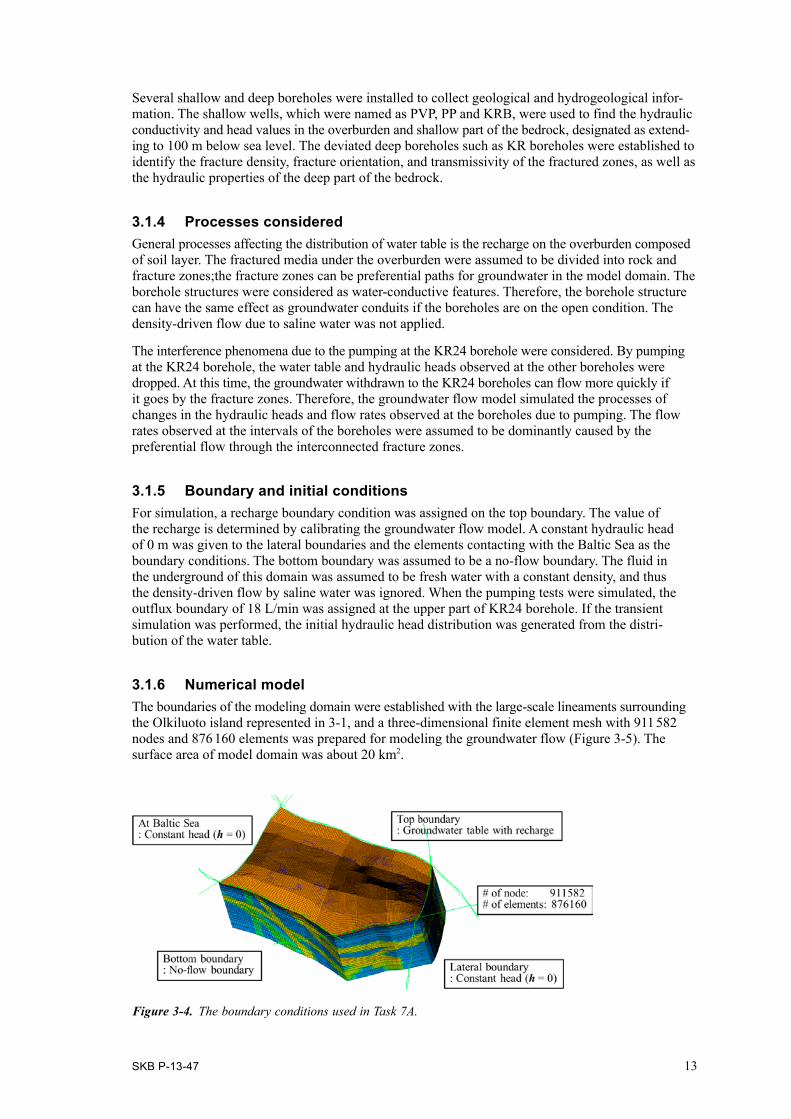
3.1.5 Boundary and initial conditionsFor simulation, a recharge boundary condition was assigned on the top boundary. The value of the recharge is determined by calibrating the groundwater flow model. A constant hydraulic head of 0 m was given to the lateral boundaries and the elements contacting with the Baltic Sea as the boundary conditions. The bottom boundary was assumed to be a no-flow boundary. The fluid in the underground of this domain was assumed to be fresh water with a constant density, and thus the density-driven flow by saline water was ignored. When the pumping tests were simulated, the outflux boundary of 18 L/min was assigned at the upper part of KR24 borehole. If the transient simulation was performed, the initial hydraulic head distribution was generated from the distri-bution of the water table.

3.1.6 Numerical modelThe boundaries of the modeling domain were established with the large-scale lineaments surrounding the Olkiluoto island represented in 3-1, and a three-dimensional finite element mesh with 911 582 nodes and 876 160 elements was prepared for modeling the groundwater flow (Figure 3-5). The surface area of model domain was about 20 km2.

Figure 3-4. The boundary conditions used in Task 7A.

14 SKB P-13-47

The heterogeneous and anisotropic hydraulic conductivities were assigned to each cell in the mesh through the following steps. First, a discrete fracture network was constructed with the fractured zones that were identified as water conductive features from the field investigations such as geophysical survey, geological mapping and borehole investigation (Figure 3-5). Transmissivity of each fractured zone was assumed to be a constant as measured (shown in Figure 3-5a). Then, we constructed the EPM domain and calculated its anisotropic hydraulic conductivity field from the DFN of fracture zones using Oda’s method (Oda 1985). When the hydraulic gradient, i̶, is induced in an element, the hydraulic gradient induced in a fracture, whose normal vector is n̶ , is given by i̶ – n̶ nT̶ i̶. If the fracture transmissivity, Tf, is isotropic, the flux in the fracture, q̶ f , is given by Darcy’s law, and sizes of the fracture and element as follows:

( )f Tf

ATq K i I nn i

V= − ⋅ = − ⋅ (3-1)

where A is the area of the fracture, V is the volume of the element, and I̶ is the identity matrix.

The net flux in the element can be derived by summing the flux in fractures in the element, and the net hydraulic conductivity tensor by fractures can be determined from the derived net flux. Then, the determined tensor is combined with the hydraulic conductivity tensor of rock matrix that was assumed as an isotropic medium with the hydraulic conductivity of 1.0 × 10−11 m/s. Note that the assumption of the hydraulic property of the matrix is based on field observations. Finally, the calculated hydraulic conductivity tensors for the whole elements were assigned to the equivalent continuum medium domain (Figure 3-5b).

With the established hydraulic conductivity field, FEFLOW, a finite element subsurface flow and transport simulation model, was applied to solve the groundwater flow problem (Diersch 2005a). To consider the effects of boreholes on the groundwater flow, a “discrete fracture element” approach was used (Diersch 2005b). In this approach, the open and packed-off boreholes can be conceptualized

Figure 3-5. (a) The fracture network and (b) the hydraulic conductivity distribution of the groundwater flow model.

SKB P-13-47 15

as the independent finite elements with lower dimensionality at existing nodes located at the position of the slanted borehole. The fluid flow in discrete fracture elements, representing the flow within the borehole, was assumed to follow the Hagen–Poiseuille equation for laminar flow in a cylindrical pipe. The hydraulic conductivity of the element was given by the diameter of each borehole as follows (Diersch 2005b):

21 3

12 2elemgK Rρ

µ

= (3-2)

where Kelem is the hydraulic conductivity of the borehole element, ρ and μ are the density and dynamic viscosity of the fluid, respectively, g is the gravitational acceleration, and R is the radius of the borehole.

3.1.7 ParametersThe hydraulic conductivities of the rock media and fracture zones were measured in the field con-dition and used in the groundwater flow model (Figure 3-5a) The radius of all the boreholes was 75.5 mm. The recharge rate and hydraulic conductivity of the overburden were adjusted by calibrating the regional-scale groundwater flow model.

3.1.8 Model conditioning and calibration For the groundwater flow system of the study site, two conditions were simulated. First, under the assumption of steady state, groundwater flow in a natural condition, where no artificial stress was applied to the groundwater flow system, was simulated. Then, the stabilized groundwater flow to a long-term pumping test was simulated (Vaittinen and Ahokas 2005). For simulation of the two con-ditions, the hydraulic conductivity of overburden and recharge rate were calibrated by minimizing the root mean square errors (RMSEs) between the simulated and measured heads at the boreholes with an optimization process using a genetic algorithm. The RMSEs were calculated by the follow equation:

( )2

1

1RMSEn

cal obsi i

ih h

n =

= −∑ (3-3)

where n is the number of observation points, hical is the hydraulic heads simulated by the model at

the i-th observation point, and hiobs is the hydraulic heads measured in the field at the i-th observation

point. The genetic algorithm used for calibration is an attempt to find an optimum by analogy with the evolutionary update of the gene (Gershenfeld 1999). It has been widely used in various optimization and parameter estimation problems for groundwater flow (Freeze and Gorelick 1999). The decision variables were the hydraulic conductivity of the overburden and recharge rate, and optimal decision variables which minimize the RMSEs were found by the genetic algorithm. Note that the hydraulic heads and drawdowns used in calibration were observed at the open and packed-off boreholes in the site.

3.2 Task 7B3.2.1 Modelling approachThe objective of modeling in Task 7B is to understand the block scale groundwater flow system in regards to flow and head responses. The groundwater flow model was constructed to simulate the KR14–18 cross-borehole interference tests conducted in the Olkiluoto field condition. In the simula-tion of the groundwater flow for a fractured rock, large fracture zones were used to construct a main fracture network. Then, a rock domain was represented by hybrid approach with spatially variable hydraulic conductivity values obtained from background fractures observed in the study site. The groundwater flow models constructed by the hybrid approach were calibrated with the hydraulic head data observed in the study site and the suitability of the adjusted parameters was examined by the flow rate data measured in the boreholes. Finally, the groundwater pathways were simulated.

16 SKB P-13-47

3.2.2 Data usage and interpretation The geometry data of the modelling site and fracture zones, and the statistics of the background frac-tures were obtained from dxf files and the memo of geohydrological model for the repository layout planning and numerical flow simulations. From the measurement data sheets, the three-dimensional monitoring positions at the boreholes were identified. The hydraulic heads were used to calibrate the groundwater flow model, and the flow rates observed in the intersection between the boreholes and fractures were used to compare the simulation results from the model and the measurements in the field site.

From the statistics of the background fractures, the unconditional background fracture distributions were generated using the extent and orientation distributions obtained from the analysis of the back-ground fractures observed in the boreholes.

3.2.3 Geometrical descriptionThe study area is located at the centre of the Olkiluoto island (Figure 3-6). Several fractured zones with different magnitudes and orientations, including major fractures with N-S and E-W strikes, were checked from field and drilling core investigation (Anttila et al. 1999). The area of the block-scale groundwater flow domain was 500 m × 500 m and the depth of the domain was 600 m from the sea level. The shallow and deep observation boreholes, named as KRB (KR15B–KR18B) and KR (KR14–KR18), respectively, were located at the central part of the domain (Figure 3-6). Some large fracture zones including HZ19 and HZ20 were identified at the boreholes installed in this domain.

3.2.4 Processes consideredThe pumping tests were performed at KR14 and KR18, when the boreholes were in both open and packed-off conditions (Rouhiainen and Pöllänen 2003, Klockars et al. 2006). When boreholes were in the open condition, the boreholes opened from bottom to top, and cross-flow among the fracture zones intersecting the boreholes was possible. In the packed-off condition, each observation interval in the boreholes was isolated and cross-flow was interrupted. For the three situations of natural con-ditions and pumping at the KR 14 and KR18 boreholes, the hydraulic heads in the open boreholes and at the isolated intervals of the packed-off boreholes were observed by Posiva Oy during the interference pumping tests (Rouhiainen and Pöllänen, 2003, Klockars et al. 2006).

3.2.5 Boundary and initial conditionsThe lateral and bottom boundaries of the domain were assumed as constant head conditions with head values from the results of regional groundwater flow simulation for whole of the Olkiluoto island performed in the Task 7A (Ko et al. 2012). The initial condition of the hydraulic head distribu-tion was also designated from the regional modeling results by Ko et al. (2012). When the pumping tests were simulated, the pumping rates were assigned at the pumping wells, 25 L/min at the KR14 and 6 L/min at the KR18, respectively. The recharge rate into the top layer of the model domain was assumed and adjusted by calibrating the groundwater flow model.

3.2.6 Numerical modelA three-dimensional mesh with 862 272 nodes and 838 660 elements was prepared to simulate the groundwater flow in the modeling domain, the central part of the Olkiluoto island. The observation boreholes were located in the central part of the domain.

Generally, the hydraulic conductivity distributions used in the modelling of Task 7B were constructed using the same method as in Task 7A without considering the background fractures: the rock domain had the same hydraulic conductivity values as in Task 7A.

SKB P-13-47 17

Several large fracture zones were identified from the survey of the outcrops and borehole logging data (Ahokas et al. 2007). Furthermore, the background fractures were observed from the logging data (Ahokas et al. 2007, Posiva 2009) and their statistical properties were analyzed (Ko et al. 2010). From the background fracture analysis, unconditional realizations of the background fractures were generated (Figure 3-8). The unconditional realizations of the background fracture distribution, in which the statistics of orientations and extents of the background fractures were only considered, were generated using the field measurement data (Posiva 2009).

Finally, the entire discrete fracture network was constructed. by deterministically including the large fracture zones and stochastically inserting the background fractures. Oda’s method was employed to input the hydraulic conductivity distributions of the major fracture zones and background fractures into the groundwater flow models discretized by finite element meshes, given in Figure 3-8c (Oda 1985, Ko et al. 2010). To find the solution for the groundwater flow system of the three-dimensional continuum mesh with the heterogeneous hydraulic conductivity field by finite element method, FEFLOW (Diersch 2005a) was used. Then, a discrete fracture element approach was used to reflect the effect of the borehole structures on the groundwater flow system (Diersch 2005b).

3.2.7 ParametersFrom the reports for the Olkiluoto site, the transmissivity of the large fracture zones were measured in the field condition and used in the groundwater flow model (shown in Figure 3-8a). The data for the background fractures were analysed and their statistics were used to generate the unconditional background fracture distributions (Ko et al. 2010). The radius of the boreholes was 75.5 mm. The recharge rate was adjusted by calibrating the block-scale groundwater flow model.

Figure 3-6. Location of the study site, with the observation boreholes and modeling domain included in the dotted rectangle (after Pitkänen et al. 2007 and Posiva 2009).

Figure 3-7. The boundary conditions used in Task 7B.

18 SKB P-13-47

Figure 3-8. (a) The large fracture network, (b) the background fractures, and (c) the hydraulic conductivity distribution of the groundwater flow model.

(a)

(b)

(b)

(c)

SKB P-13-47 19

3.2.8 Model conditioning and calibrationIn the calibration of the block-scale groundwater flow model, the recharge rate was controlled. The six groundwater flow simulations were used to calibrate the groundwater flow models,. Two condi-tions of the boreholes (open and packed-off) and three situations of the hydraulic stress events (no pumping, pumping at KR14, and pumping at KR18) were simultaneously involved.

The calibrated parameters were obtained by minimizing the total sum of squared errors (SSEs) between the simulated and measured heads in the boreholes for the six simulations. The response function between the recharge rate and SSE for each simulation was estimated by calculating the SSE with various recharge rates. Then, the total SSEs for various recharge rates were calculated by summing up the response functions of six simulations as shown in Figure 4-15. With the graph of the total SSEs and recharge rates, the optimal parameter appropriately representing the six ground water flow simula-tions simultaneously was determined. For a single modeling domain, the total SSE was calculated by the following equation:

( )6 2

, ,1 1

Total SSEin

cal obsi j i j

i jh h

= =

= −∑∑ (3-4)

where nobs is the total number of observation points for all simulations; ni is the number of observation points for i-th simulation; hi,j

cal is the hydraulic heads simulated at the j-th observation point for the i-th simulation; hi,j

obs is the hydraulic heads measured in the field at the j-th observation point for the i-th simulation.

3.3 Task 7C3.3.1 Modelling approachThe objective of simulations in Task 7C was to consider the way to examine groundwater flow in a single fracture using groundwater flow data of hydraulic tests in field conditions. In order to achieve this objective, a single fracture identified at the underground facility located in Olkiluoto island was used. The groundwater flows were measured at the intersections between the single fracture and several boreholes. Transmissivity values at the intersection were geostatistically analyzed and the interpolated transmissivity field from a kriging method was used to simulate the groundwater flow rates between the single fracture and the boreholes. Then, random realizations of the transmissivity field with the same spatial correlation and statistical properties to the interpolated field were generated for examining the uncertainty surround-ing the simulation results. The two-dimensional forward groundwater flow modeling was used.

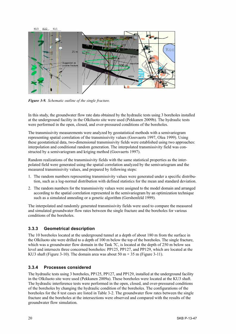
3.3.2 Data usage and interpretation By investigating the drilling core from the 10 boreholes installed at the underground tunnel, a single fracture, which intersected with all boreholes, was identified (Pekkanen 2009a) (Figure 3-9). The transmissivity values of the single fracture at the positions where the boreholes were crossed were measured (Table 3-1).

Table 3-1. Transmissivity values measured at the intersections between the single fracture and the boreholes (Pekkanen 2009a, b).

Borehole X (m) Y (m) Depth (m) Transmissivity (m2/s) Shaft

PP134 1 525 919.91 6 791 991.53 −250.64 5.49 × 10−10 KU1KR38 1 525 902.32 6 792 015.59 −248.09 1.16 × 10−8 KU2PP122 1 525 901.09 6 792 015.15 −247.39 1.46 × 10−9

PP123 1 525 901.69 6 792 014.57 −247.49 1.41 × 10−9

PP124 1 525 901.80 6 792 013.78 −247.49 4.21 × 10−9

PP126 1 525 904.02 6 792 015.04 −248.69 4.30 × 10−9

PP128 1 525 903.00 6 792 016.59 −248.59 1.12 × 10−9

PP125 1 525 926.96 6 791 972.92 −254.31 9.47 × 10−11 KU3PP127 1 525 924.99 6 791 975.02 −254.91 2.03 × 10−10

PP129 1 525 923.67 6 791 973.23 −253.41 9.47 × 10−11

20 SKB P-13-47

In this study, the groundwater flow rate data obtained by the hydraulic tests using 3 boreholes installed at the underground facility in the Olkiluoto site were used (Pekkanen 2009b). The hydraulic tests were performed in the open, closed, and over-pressured conditions of the boreholes.

The transmissivity measurements were analyzed by geostatistical methods with a semivariogram representing spatial correlation of the transmissivity values (Goovaerts 1997, Olea 1999). Using these geostatistical data, two-dimensional transmissivity fields were established using two approaches: interpolation and conditional random generation. The interpolated transmissivity field was con-structed by a semivariogram and kriging method (Goovaerts 1997).

Random realizations of the transmissivity fields with the same statistical properties as the inter-polated field were generated using the spatial correlation analyzed by the semivariogram and the measured transmissivity values, and prepared by following steps:

1. The random numbers representing transmissivity values were generated under a specific distribu-tion, such as a log-normal distribution with defined statistics for the mean and standard deviation.

2. The random numbers for the transmissivity values were assigned to the model domain and arranged according to the spatial correlation represented in the semivariogram by an optimization technique such as a simulated annealing or a genetic algorithm (Gershenfeld 1999).

The interpolated and randomly generated transmissivity fields were used to compare the measured and simulated groundwater flow rates between the single fracture and the boreholes for various conditions of the boreholes.

3.3.3 Geometrical descriptionThe 10 boreholes located at the underground tunnel at a depth of about 180 m from the surface in the Olkiluoto site were drilled to a depth of 100 m below the top of the boreholes. The single fracture, which was a groundwater flow domain in the Task 7C, is located at the depth of 250 m below sea level and intersects three concerned boreholes: PP125, PP127, and PP129, which are located at the KU3 shaft (Figure 3-10). The domain area was about 50 m × 35 m (Figure 3-11).

3.3.4 Processes consideredThe hydraulic tests using 3 boreholes, PP125, PP127, and PP129, installed at the underground facility in the Olkiluoto site were used (Pekkanen 2009a). These boreholes were located at the KU3 shaft. The hydraulic interference tests were performed in the open, closed, and over-pressured conditions of the boreholes by changing the hydraulic condition of the boreholes. The configurations of the boreholes for the 8 test cases are listed in Table 3-2. The groundwater flow rates between the single fracture and the boreholes at the intersections were observed and compared with the results of the groundwater flow simulation.

Figure 3-9. Schematic outline of the single fracture.

SKB P-13-47 21

Figure 3-10. Schematic diagram of the interference test in Task 7C when PP125 was open and other boreholes were closed.

Figure 3-11. The groundwater flow model domain used in Task 7C.

22 SKB P-13-47

Table 3-2. Configurations of the hydraulic tests performed at the PP-125, PP127, and PP129 boreholes (h means a hydraulic head of the borehole used in the groundwater flow simulation).

Case Observation borehole

Borehole conditions

PP125 PP127 PP129

1 PP125 open (h = −176.81 m) closed closed2 PP127 closed open (h = −176.81 m) closed3 PP125 open (h = −176.81 m) open (h = −176.81 m) closed4 PP125 open (h = −176.81 m) closed open (h = −176.81 m)5 PP127 open (h = −176.81 m) open (h = −176.81 m) over-pressured (h = −156.60 m)6−1 PP125 open (h = −176.81 m) open (h = −176.81 m) open (h = −176.81 m)6−2 PP127 open (h = −176.81 m) open (h = −176.81 m) open (h = −176.81 m)6−3 PP125 open (h = −176.81 m) open (h = −176.81 m) open (h = −176.81 m)

3.3.5 Boundary and initial conditionsThe boundary conditions of four sides were assigned as constant head boundaries and obtained from the results of the regional and local scale groundwater flow simulations (Ko et al. 2010, 2012). According to the conditions of the boreholes, which were opened or over-pressured, specific boundary conditions were applied at the locations of the boreholes. If the boreholes were closed, there was no boundary condition, in order to assign no outflow to the borehole and maintain groundwater pressure at the location. When the boreholes were open, it was supposed that the hydraulic heads at the top of the boreholes were developed constantly. The equivalent hydraulic head to the given pressure was added at the over-pressured borehole as a constant head boundary like an open condition.

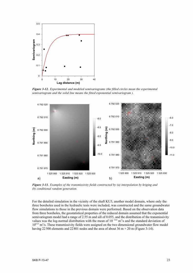
3.3.6 Numerical modelTo construct two-dimensional transmissivity fields used in the simulation of groundwater flow, the measurements of the transmissivity at the boreholes were analyzed using a geostatistical approach. From the distance among the boreholes and the measurements, the experimental semivariogram of the transmissivity was constructed (Figure 3-12) and an exponential semivariogram model with the range of 15.0 m and the sill of 0.4 was selected as given in Equation (3-5).

( ) ( )( )3 /15.00.4 1 hh eγ −= − (3-5)

where γ(h) is the semivariogram, h is the lag distance (m).

Using the selected semivariogram model and kriging method, the interpolated transmissivity field was prepared (Figure 3-13). The transmissivity values were high at the part of KU2, and became lower as the KU3 was reached.

The realizations of the transmissivity fields were generated and applied to the groundwater flow model, and the flow rates between the boreholes and the single fractures were calculated for evaluating the uncertainty in the results of the groundwater flow rates. The distribution of the transmissivity values was assumed to be log-normal with the mean of 10−9.0 m2/s and the standard deviation of 100.63 m2/s from the analysis of the transmissivity measurements. The random variables under the distribution and the simulated annealing technique, which arranged the transmissivity values to the groundwater flow model domain according to the analyzed semivariogram, were used to construct the transmis-sivity fields. Therefore, the transmissivity fields with the same statistical properties and spatial correlation to the interpolated field were generated.

These transmissivity fields were assigned to the two dimensional groundwater flow model domain having 3 796 elements and 3 922 nodes and the groundwater flow simulations were conducted.

SKB P-13-47 23

Figure 3-12. Experimental and modeled semivariograms (the filled circles mean the experimental semivariogram and the solid line means the fitted exponential semivariogram ).

0 10 20 30 40Lag distance (m)

0

0.1

0.2

0.3

0.4

0.5

Sem

ivar

iogr

am

Figure 3-13. Examples of the transmissivity fields constructed by (a) interpolation by kriging and (b) conditional random generation.

1 525 900 1 525 910 1 525 920 1 525 930

Easting (m)

6 791 970

6 791 980

6 791 990

6 792 000

6 792 010

6 792 020

Nor

thin

g (m

)

-10.0

-9.5

-9.0

-8.5

-8.0

1 525 900 1 525 910 1 525 920 1 525 930

Easting (m)

6 791 970

6 791 980

6 791 990

6 792 000

6 792 010

6 792 020N

orth

ing

(m)

-11.0

-10.0

-9.0

-8.0

-7.0

-6.0

a) b)

For the detailed simulation in the vicinity of the shaft KU3, another model domain, where only the three boreholes used in the hydraulic tests were included, was constructed and the same groundwater flow simulations to those in the previous domain were performed. Based on the observation data from three boreholes, the geostatistical properties of the reduced domain assumed that the exponential semivariogram model had a range of 2.55 m and sill of 0.055, and the distribution of the transmissivity values was the log-normal distribution with the mean of 10−10.0 m2/s and the standard deviation of 100.23 m2/s. These transmissivity fields were assigned on the two dimensional groundwater flow model having 22 500 elements and 22 801 nodes and the area of about 36 m × 20 m (Figure 3-14).

24 SKB P-13-47

3.3.7 ParametersTransmissivity values were determined from the data represented in the documents from the Task Force for the field measurement of the interference tests. The geostatistical statistics were yielded from the transmissivity data. The effect of the borehole structures was not considered.

3.3.8 Model conditioning and calibrationNo action was taken to calibrate the two-dimensional groundwater flow model using the flow rate data obtained from the field tests. Only the comparisons between the simulated and measured flow rates were carried out.

Figure 3-14. Transmissivity fields constructed by (a) interpolation by kriging and (b) random generation in the reduced model domain.

SKB P-13-47 25

4 Results

4.1 Task 7ATable 4-1 shows the list of groundwater flow simulations conducted in Task 7A.

Table 4-1. Simulation list performed in Task 7A.

Name Description Remarks Boreholes

SS02a Steady state flow condition with open borehole Forward Boreholes are open and free to cross-flowSS02b Steady state flow condition with open borehole Calibration Boreholes are open and free to cross-flowSS02c Steady state flow condition without pumping Forward No boreholesSS04a Steady state flow with extraction from KR24 Forward KR24 + monitoring boreholesSS04b Steady state flow with extraction from KR24 Calibration KR24 + monitoring boreholesPA01 PA condition simulation Forward No boreholesTR02a Transient flow with extraction from KR24 Forward KR24 + monitoring boreholesTS10a Transient flow with extraction from KR24

– calibration to head measurement onlyCalibration KR24 + monitoring boreholes

SS11 Steady state flow condition with open borehole Forward Boreholes are open and free to cross-flowSS13 Steady state flow condition without pumping Forward No boreholesPA10 PA condition simulation Forward No boreholes

Figure 4-1 shows measured and simulated hydraulic heads from simulations SS02b (with boreholes) and SS02c (without boreholes). The simulated heads in SS02b show good agreement with the meas-ured heads with the exception of the deeper parts of KR09 and KR12. The model assumed a constant fluid density of 1 000 kg/m3 and so did not reproduce the high heads at depths below −500 m from the sea level because it did not include the observed salinity profile. The effect of the boreholes is clearly seen, by comparing the two simulations. In the model without boreholes, hydraulic heads are increased in the upper part of the models while heads decrease significantly in the lower part. In part this may be a result of the lateral constant head boundaries assumed, but it also reflects the ability of the boreholes to disturb the natural head field due to their high vertical transmissivity suggesting that the DFE method can successfully describe the open borehole effects.

Figure 4-2 shows the measured and simulated drawdowns in SS04a and SS04b. Drawdowns are typi-cally slightly lower in the calibrated model (SS04b) with higher recharge. The difference between the measured and simulated drawdowns is relatively large even with the increased recharge and adjust-ments to the structural model (e.g. inclusion of zone heterogeneity) would be required to achieve a better match.

In the comparisons of the flow rates, the match to flow magnitude and direction is generally reason-able, but some major flow features in KR28 are not predicted by the simulations (Figure 4-3).

Transient simulations were performed using the SS04b calibration assuming a calibrated storage coefficient of 10−7 m−1. Reasonable matches were achieved to the source interval in KR24 and monitoring zones as shown in Figure 4-4. The difference between steady state drawdowns and those calculated at the end of pumping in the transient models were small due to the small storage coefficient (Figure 4-5).

Simulations SS11 and SS13 used the results of the calibrated models to consider the differences due to the presence of the boreholes. They clearly show the strong effect of the boreholes on the observed head field. The effect of open boreholes should be considered for calibration of the groundwater flow model for a fractured rock aquifer with low permeable matrix.

26 SKB P-13-47

Figure 4-1. Measured and simulated hydraulic heads for selected boreholes in SS02b and c.

KR1-1000

-800

-600

-400

-200

0

Elev

atio

n (m

)0 2 4 6 8 10 12

Head (m)

-1000

-800

-600

-400

-200

00 2 4 6 8 10 12

-1000

-800

-600

-400

-200

00 2 4 6 8 10 12

-1000

-800

-600

-400

-200

00 2 4 6 8

-1000

-800

-600

-400

-200

00 2 4 6 8 10 12

-1000

-800

-600

-400

-200

00 2 4 6 8 10 12

-1000

-800

-600

-400

-200

00 2 4 6 8 10 12

-1000

-800

-600

-400

-200

00 2 4 6 8 10 12

-1000

-800

-600

-400

-200

00 2 4 6 8 10 12 14

Elev

atio

n (m

)

Head (m)

Elev

atio

n (m

)

Head (m)El

evat

ion

(m)

Head (m)El

evat

ion

(m)

Head (m)

Elev

atio

n (m

)

Head (m)

Elev

atio

n (m

)

Head (m)

Elev

atio

n (m

)

Head (m)El

evat

ion

(m)

Head (m)

KR23 KR25

KR24 KR3 KR5

KR9 KR11 KR12

MeasuredSS02bSS02c

MeasuredSS02bSS02c

MeasuredSS02bSS02c

MeasuredSS02bSS02c

MeasuredSS02bSS02c

MeasuredSS02bSS02c

MeasuredSS02bSS02c

MeasuredSS02bSS02c

MeasuredSS02bSS02c

SKB P-13-47 27

Figure 4-2. Measured and simulated drawdowns for selected boreholes in SS04a and b.

-1000

-800

-600

-400

-200

0-2 0 2 4 6 8 10

-1000

-800

-600

-400

-200

00 2 4 6 8 10 12

-1000

-800

-600

-400

-200

00 2 4 6 8 10 12

-1000

-800

-600

-400

-200

00 5 10 15 20

-1000

-800

-600

-400

-200

0-2 0 2 4 6 8 10

-1000

-800

-600

-400

-200

0-2 0 2 4 6 8 10

-1000

-800

-600

-400

-200

0-2 0 2 4 6 8 10

-1000

-800

-600

-400

-200

0-4 -2 0 2 4 6 8

-1000

-800

-600

-400

-200

00 2 4 6 8 10 12 14

Elev

atio

n (m

)

Elev

atio

n (m

)

Elev

atio

n (m

)

Elev

atio

n (m

)

Elev

atio

n (m

)

Elev

atio

n (m

)

Elev

atio

n (m

)

Elev

atio

n (m

)

Elev

atio

n (m

)

Drawdown (m) Drawdown (m) Drawdown (m)

Drawdown (m) Drawdown (m) Drawdown (m)

Drawdown (m) Drawdown (m) Drawdown (m)

KR1 KR23 KR25

KR24 KR3 KR5

MeasuredSS04aSS04b

MeasuredSS04aSS04b

MeasuredSS04aSS04b

MeasuredSS04aSS04b

MeasuredSS04aSS04b

MeasuredSS04aSS04b

MeasuredSS04aSS04b

MeasuredSS04aSS04b

MeasuredSS04aSS04b

KR9 KR11 KR12

28 SKB P-13-47

Figure 4-4. Measured and simulated transient hydraulic heads for TR10a simulation.

Figure 4-3. Measured and simulated predicted flow rates for pumping in KR24.

0 40 80 120Elapsed time (days)

-15

-10

-5

0

5

10

Hea

d (m

)

KR24U_MeasuredKR24U_SimulatedKR24L_MeasuredKR24L_Simulated

0 40 80 1200

2

4

6

8

10

KR07_MeasuredKR07_SimulatedKR10_MeasuredKR10_SimulatedKR22_MeasuredKR22_Simulated

0 40 80 1200

2

4

6

8

10

KR01_T7_MeasuredKR01_T7_SimulatedKR23_T6_MeasuredKR23_T6_SimulatedKR25_T3_MeasuredKR25_T3_SimulatedKR25_T2_MeasuredKR25_T2_Simulated

Hea

d (m

)

Hea

d (m

)

Elapsed time (days) Elapsed time (days)

Elev

atio

n (m

)

-500

-400

-300

-200

-100

0-10 -5 0 5 10

Flow rate (m3/day)

KR4-500

-400

-300

-200

-100

0-5 0 5

-500

-400

-300

-200

-100

0-20 -10 0 10 20

-500

-400

-300

-200

-100

0-20 -10 0 10 20

-500

-400

-300

-200

-100

0-20 -10 0 10 20

Elev

atio

n (m

)

Flow rate (m3/day) Flow rate (m3/day)El

evat

ion

(m)

Elev

atio

n (m

)

Elev

atio

n (m

)

Flow rate (m3/day) Flow rate (m3/day)

KR27 KR28

KR22KR14

MeasuredSS04aSS04b

MeasuredSS04aSS04b

MeasuredSS04aSS04b

MeasuredSS04aSS04b

MeasuredSS04aSS04b

SKB P-13-47 29

Figure 4-5. Comparisons of the drawdown in the steady state modelling and the transient modelling at the end of pumping.

Drawdown (m)

-1000

-800

-600

-400

-200

0-2 0 2 4 6 8 10

-1000

-800

-600

-400

-200

00 2 4 6 8 10 12

-1000

-800

-600

-400

-200

00 2 4 6 8 10 12

-1000

-800

-600

-400

-200

00 5 10 15 20

-1000

-800

-600

-400

-200

0-2 0 2 4 6 8 10

-1000

-800

-600

-400

-200

0-2 0 2 4 6 8 10

-1000

-800

-600

-400

-200

0-2 0 2 4 6 8 10

-1000

-800

-600

-400

-200

0-4 -2 0 2 4 6 8

-1000

-800

-600

-400

-200

0-2 0 2 4 6 8 10 12

KR1 KR23 KR25

KR24 KR3 KR5

KR9 KR11 KR12

Elev

atio

n (m

)El

evat

ion

(m)

Elev

atio

n (m

)

Elev

atio

n (m

)El

evat

ion

(m)

Elev

atio

n (m

)

Elev

atio

n (m

)El

evat

ion

(m)

Elev

atio

n (m

)

MeasuredSS04bTS10a

MeasuredSS04bTS10a

MeasuredSS04bTS10a

MeasuredSS04bTS10a

MeasuredSS04bTS10a

MeasuredSS04bTS10a

MeasuredSS04bTS10a

MeasuredSS04bTS10a

MeasuredSS04bTS10a

Drawdown (m) Drawdown (m)

Drawdown (m) Drawdown (m) Drawdown (m)

Drawdown (m) Drawdown (m) Drawdown (m)

30 SKB P-13-47

Particle transport calculations were performed using the SS02b and SS13 flow fields assuming a uniform subsurface porosity of 5 % which was from Freeze and Cherry (1979). The transport paths from the three release points are shown in Figure 4-7. The transport paths appear to be identical in the two simulations. Travel time is approximately 10 % lower in that using the SS13 flow model.

Figure 4-6. Simulated heads for SS11 and 13.

SS11SS13

-1000

-800

-600

-400

-200

00 2 4 6 8 10 12

-1000

-800

-600

-400

-200

00 2 4 6 8 10 12

-1000

-800

-600

-400

-200

00 2 4 6 8 10 12

-1000

-800

-600

-400

-200

00 2 4 6 8

-1000

-800

-600

-400

-200

00 2 4 6 8 10 12

-1000

-800

-600

-400

-200

00 2 4 6 8 10 12

-1000

-800

-600

-400

-200

00 2 4 6 8 10 12

-1000

-800

-600

-400

-200

00 2 4 6 8 10 12

-1000

-800

-600

-400

-200

00 2 4 6 8 10 12 14

Elev

atio

n (m

)El

evat

ion

(m)

Elev

atio

n (m

)

Elev

atio

n (m

)El

evat

ion

(m)

Elev

atio

n (m

)

Elev

atio

n (m

)El

evat

ion

(m)

Elev

atio

n (m

)

Head (m) Head (m) Head (m)

Head (m) Head (m) Head (m)

Head (m) Head (m) Head (m)

KR23 KR25

KR24 KR3 KR5

KR9 KR11 KR12

KR1

SS11SS13

SS11SS13

SS11SS13

SS11SS13

SS11SS13

SS11SS13

SS11SS13

SS11SS13

Figure 4-7. (a) Plan and (b) section view of transport path for SS02b and SS13 flow models.

SKB P-13-47 31

4.2 Task 7B

Table 4-2 shows the list of groundwater flow simulations conducted in Task 7B.

Under natural conditions in the boreholes, the hydraulic heads simulated under the stochastic con-tinuum approach showed good agreement in matching the simulated and measured data, especially in the case of the packed-off borehole condition (Figure 4-8). From the small standard deviations of the hydraulic heads, it was thought that the stochastic background fractures had little influence on the variation of the heads, and the boundary conditions from the regional groundwater flow modeling still gave dominant effect to the simulation results though the added available conduits were effective in the packed-off boreholes condition. The calibrated recharge rates in the open and packed-off conditions were 6.6 mm/yr and 0.4 mm/yr and their standard deviations were 0.5 mm/yr and 0.1 mm/yr, respectively. The relatively high recharge rate for the open condition resulted in similar simulated heads at the boreholes due to their high transmissivity.

Figure 4-8. Simulated hydraulic heads of the steady state modelling for the natural condition in SS21 and 22: (a) open and (b) packed-off borehole conditions (the bar sticking to the data points means the standard deviation from the generated realizations).

4 5 6 7 8 9Measured (m)

4

5

6

7

8

9

Sim

ulat

ed (m

)

KR14KR15KR16KR17KR18KR15BKR16BKR17BKR18B

4 5 6 7 84

5

6

7

8

KR14KR15KR16KR17KR18KR15BKR16BKR17BKR18B

a) b)

Sim

ulat

ed (m

)

Measured (m)

32 SKB P-13-47

The discrepancy in flow rates of the boreholes between measurements and simulated results was also relatively low (Figure 4-9). The exaggerated flow rates at the points where the deterministic fracture zones were crossed were relaxed. The variations of the flow rates, represented by the standard devia-tions, were relatively small for the same reason as in the case of hydraulic heads.

The pathways obtained by the particle tracking simulations are represented in Figure 4-10. Due to the boundary condition, the particles passed out of the model domain. Near the large fracture zones, the pathways had complex features.

Figure 4-9. Simulated flow rates of the steady state modelling for the natural condition in SS21 (positive and negative signs represent the in- and out-flux from the boreholes).

Figure 4-10. Particle tracking pathways for the selected positions in PA20c: (a) top view and (b) 3-D view.

SKB P-13-47 33

Table 4-3. Travel times and distances for each particle released from the points in PA20c.

Release Point Travel time (× 103 year) Travel distance (m)

1 10.8 ± 2.2 214 ± 32 12.1 ± 2.9 220 ± 53 21.1 ± 5.1 234 ± 94 16.7 ± 2.5 271 ± 45 25.4 ± 8.1 281 ± 396 17.7 ± 2.5 234 ± 57 47.2 ± 13.4 356 ± 148 25.0 ± 2.4 284 ± 79 19.5 ± 4.5 230 ± 7

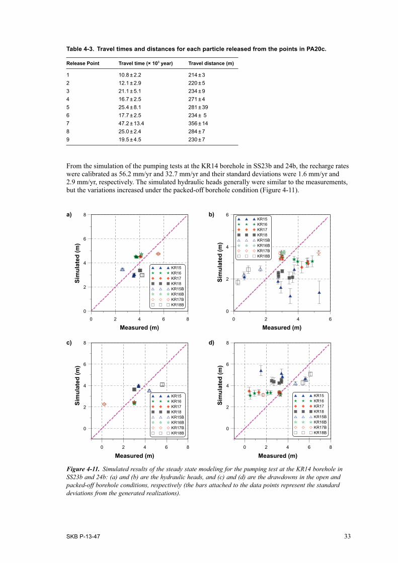
From the simulation of the pumping tests at the KR14 borehole in SS23b and 24b, the recharge rates were calibrated as 56.2 mm/yr and 32.7 mm/yr and their standard deviations were 1.6 mm/yr and 2.9 mm/yr, respectively. The simulated hydraulic heads generally were similar to the measurements, but the variations increased under the packed-off borehole condition (Figure 4-11).

Figure 4-11. Simulated results of the steady state modeling for the pumping test at the KR14 borehole in SS23b and 24b: (a) and (b) are the hydraulic heads, and (c) and (d) are the drawdowns in the open and packed-off borehole conditions, respectively (the bars attached to the data points represent the standard deviations from the generated realizations).

a) b)

c) d)

0 2 4 6 8

Measured (m)

0

2

4

6

8

Sim

ulat

ed (m

)

KR15KR16KR17KR18KR15BKR16BKR17BKR18B

0 2 4 6

0

2

4

6KR15KR16KR17KR18KR15BKR16BKR17BKR18B

0 2 4 6 8

0

2

4

6

8

KR15KR16KR17KR18KR15BKR16BKR17BKR18B

0 2 4 6 8

0

2

4

6

8

KR15KR16KR17KR18KR15BKR16BKR17BKR18B

Sim

ulat

ed (m

)

Sim

ulat

ed (m

)

Sim

ulat

ed (m

)

Measured (m)

Measured (m) Measured (m)

34 SKB P-13-47

The open boreholes led to mixing of the groundwater from each fracture zone with different hydraulic heads and decreased the contrast in hydraulic heads among the fracture zones crossing the boreholes. By the mixing effect, the differences in the different background fractures at each unconditional random realization were alleviated and the head variations were very small.

Due to packing off the observation intervals of the boreholes, the hydraulic heads at each fracture zone intersecting the boreholes could be maintained and easily influenced by the structures of background fractures which changed in each realization. Therefore, the variations of the heads and drawdown were larger in the packed-off condition than the open condition.

The flow rates simulated for the pumping tests at the KR14 borehole in SS23b showed good agree-ments with the measurement (Figure 4-12). The magnitude of local flows also appeared though the flow directions were different from the measurements at some observation points. The flow rates at the KR15 and KR16B boreholes had large standard deviations with relatively high uncertainty.

When the pumping tests at the KR18 borehole in SS25b and 26b were simulated, the recharge rates were recalibrated as 18.6 mm/yr and 15.7 mm/yr and their standard deviations were 0.8 mm/yr and 1.6 mm/yr for the open and packed-off borehole conditions, respectively. The uncertainty of the heads was represented similarly to the case of the pumping tests at the KR14 borehole (Figure 4-13).

The flow rates simulated for the pumping tests of the KR18 borehole in SS25b showed good agree-ment with the measurements, but relatively large uncertainties were obtained at KR16, KR16B, and KR18B boreholes (Figure 4-14).

Figure 4-12. Simulated flow rates of the steady state modeling the pumping test at the KR14 borehole in SS23b (positive and negative signs represent the in- and out-flux from the boreholes).

SKB P-13-47 35

Figure 4-13. Simulated results of the steady state modeling for the pumping test at the KR18 borehole in the case of background fracture: (a) and (b) are the hydraulic heads, and (c) and (d) are the drawdowns in the open and packed-off borehole conditions, respectively (the bars sticking to the data points represent the standard deviations from generated realizations).

Figure 4-14. Simulated flow rates of the steady state modeling the pumping test at the KR18 borehole in SS25b (positive and negative signs mean the in- and out-flux from the boreholes).

2 4 6 8

2

4

6

8KR14KR15KR16KR17KR15BKR16BKR17BKR18B

0 2 4 6 8

0

2

4

6

8KR14KR15KR16KR17KR15BKR16BKR17BKR18B

0 2 4 6 8

0

2

4

6

8

KR14KR15KR16KR17KR15BKR16BKR17BKR18B

0 2 4 6 8

0

2

4

6

8

KR14KR15KR16KR17KR15BKR16BKR17BKR18B

a) b)

c) d)

Measured (m)

Sim

ulat

ed (m

)

Sim

ulat

ed (m

)

Sim

ulat

ed (m

)

Sim

ulat

ed (m

)

Measured (m)

Measured (m) Measured (m)

36 SKB P-13-47

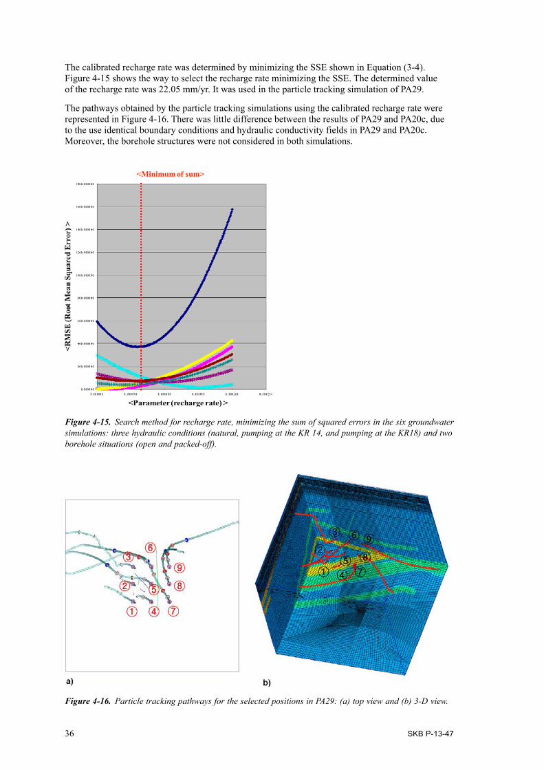
Figure 4-15. Search method for recharge rate, minimizing the sum of squared errors in the six groundwater simulations: three hydraulic conditions (natural, pumping at the KR 14, and pumping at the KR18) and two borehole situations (open and packed-off).

Figure 4-16. Particle tracking pathways for the selected positions in PA29: (a) top view and (b) 3-D view.

The calibrated recharge rate was determined by minimizing the SSE shown in Equation (3-4). Figure 4-15 shows the way to select the recharge rate minimizing the SSE. The determined value of the recharge rate was 22.05 mm/yr. It was used in the particle tracking simulation of PA29.

The pathways obtained by the particle tracking simulations using the calibrated recharge rate were represented in Figure 4-16. There was little difference between the results of PA29 and PA20c, due to the use identical boundary conditions and hydraulic conductivity fields in PA29 and PA20c. Moreover, the borehole structures were not considered in both simulations.

SKB P-13-47 37

Table 4-4. Travel times and distances for each particle released from the points in PA29.

Release Point Travel time (× 103 year) Travel distance (m)

1 8.3 ± 2.0 209 ± 22 9.0 ± 2.0 209 ± 133 17.9 ± 5.8 233 ± 124 13.5 ± 4.0 244 ± 625 16.9 ± 4.0 267 ± 66 15.0 ± 2.8 236 ± 77 52.6 ± 19.9 331 ± 238 27.3 ± 5.3 278 ± 99 15.0 ± 4.6 224 ± 7

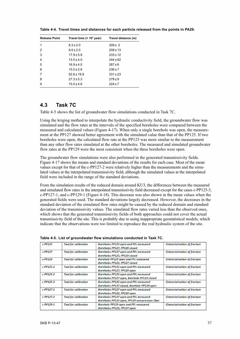
4.3 Task 7CTable 4-5 shows the list of groundwater flow simulations conducted in Task 7C.

Using the kriging method to interpolate the hydraulic conductivity field, the groundwater flow was simulated and the flow rates at the intervals of the specified boreholes were compared between the measured and calculated values (Figure 4-17). When only a single borehole was open, the measure-ment at the PP127 showed better agreement with the simulated value than that of the PP125. If two boreholes were open, the calculated flow rate at the PP125 was more similar to the measurement than any other flow rates simulated at the other boreholes. The measured and simulated groundwater flow rates at the PP129 were the most consistent when the three boreholes were open.

The groundwater flow simulations were also performed in the generated transmissivity fields. Figure 4-17 shows the means and standard deviations of the results for each case. Most of the mean values except for that of the c-PP127-2 were relatively higher than the measurements and the simu-lated values at the interpolated transmissivity field, although the simulated values at the interpolated field were included in the range of the standard deviations.

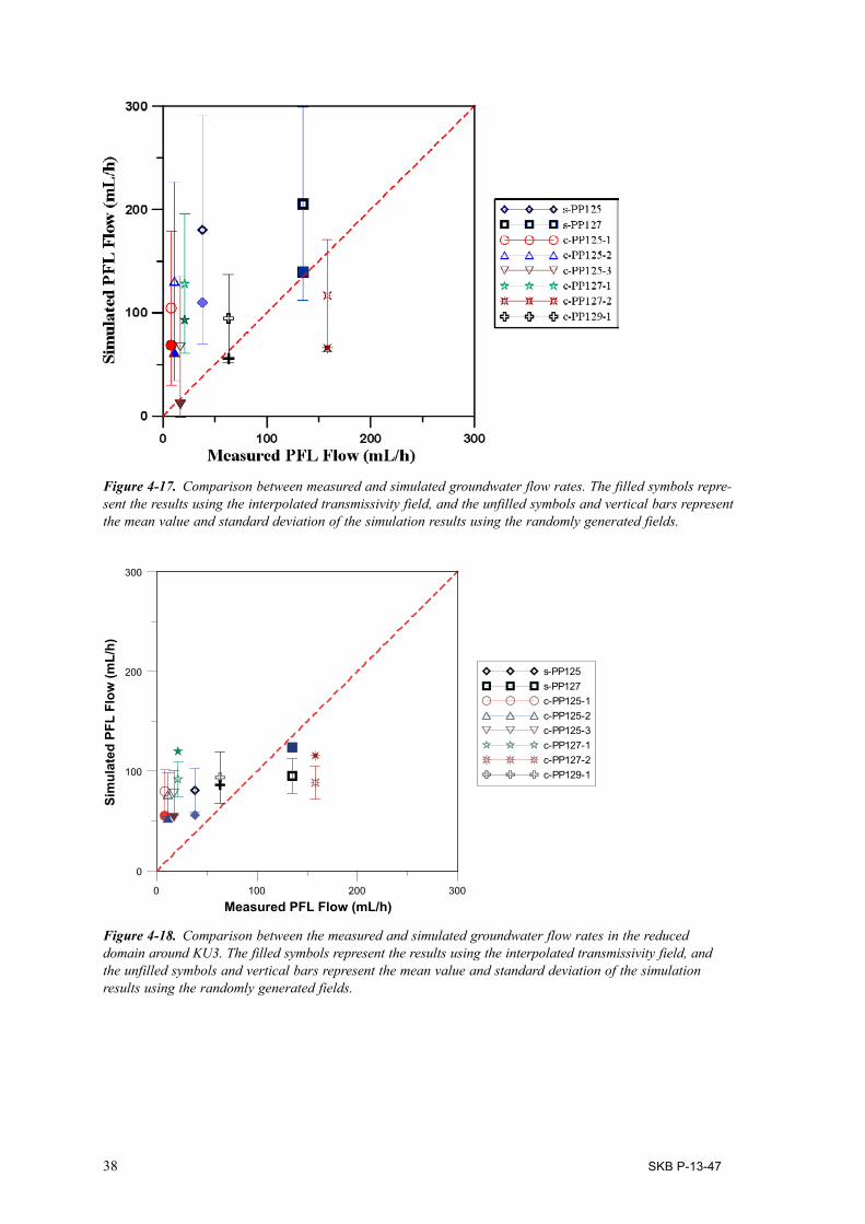
From the simulation results of the reduced domain around KU3, the differences between the measured and simulated flow rates in the interpolated transmissivity field decreased except for the cases c-PP125-3, c-PP127-1, and c-PP129-1 (Figure 4-18). This decrease was also shown in the mean values when the generated fields were used. The standard deviations largely decreased. However, the decreases in the standard deviation of the simulated flow rates might be caused by the reduced domain and standard deviation of the transmissivity values. The simulated flow rates varied less than the observed ones, which shows that the generated transmissivity fields of both approaches could not cover the actual transmissivity field of the site. This is probably due to using inappropriate geostatistical models, which indicate that the observations were too limited to reproduce the real hydraulic system of the site.

Table 4-5. List of groundwater flow simulations conducted in Task 7C.

38 SKB P-13-47

0 100 200 300

Measured PFL Flow (mL/h)

0

100

200

300

Sim

ulat

ed P

FL F

low

(mL/

h)

s-PP125s-PP127c-PP125-1c-PP125-2c-PP125-3c-PP127-1c-PP127-2c-PP129-1

Figure 4-18. Comparison between the measured and simulated groundwater flow rates in the reduced domain around KU3. The filled symbols represent the results using the interpolated transmissivity field, and the unfilled symbols and vertical bars represent the mean value and standard deviation of the simulation results using the randomly generated fields.

Figure 4-17. Comparison between measured and simulated groundwater flow rates. The filled symbols repre-sent the results using the interpolated transmissivity field, and the unfilled symbols and vertical bars represent the mean value and standard deviation of the simulation results using the randomly generated fields.

SKB P-13-47 39

5 Discussion and conclusions

5.1 Discussion of resultsIn the simulations of Task 7A, it was revealed that boreholes are likely to influence groundwater flow systems in low-permeable rock media by increasing vertical hydraulic conductivity. Calibrated groundwater flow models using steady state head data and transient head data show similar results, suggesting that the specific storage coefficient is small and should be checked in the field. The results also suggest that the uncertainty about the extent and connectivity of the fracture zones at the site requires further investigation.

In Task 7B, the simulation using the open borehole condition may not represent the pre-existing natural groundwater flow system, because the open boreholes could act as new conduits and have the same effect as pre-existing fractures on groundwater flow. A stochastic approach was required in the packed-off condition to represent the uncertainty of the groundwater flow system in fractured media by the background fractures for natural or near-natural state and in the packed-off borehole condition in this study.

The simulated values of flow rates in boreholes were reasonably well-matched to measurements from the study field, especially in relation to local groundwater flows. This showed that considering background fractures can decrease uncertainty in the results of the groundwater flow simulations by representing small variations in the model domain.

From the results of groundwater flow simulations using the interpolated and randomly generated transmissivity fields in Task 7C, the simulated flow rates were relatively higher than the measure-ments, this could be identified more clearly when the generated fields were used. These high flow rates could indicate that the values of transmissivity in the generated fields were too high and the assumption of the distribution for the transmissivity values was problematic.

In the reduced domain, the differences between the measurements and the mean values of the simulated flow rates decreased. The standard deviation also declined but this might be caused by a small number of observations (only three measurements), reduced extent of the model domain, and narrow range of the transmissivity values.

5.2 Main conclusionsThe series of groundwater flow simulations, from the regional-scale to the single fracture revealed that the borehole structures can have a significant effect on the site characterisations representing hydrogeological properties and groundwater flow systems. This effect may be emphasized if the domain concerned is comprised of sparsely fractured rock masses because the borehole structure can provide conduits for groundwater which did not exist in natural circumstances.

The local conductive features of the rock domain are also very important for identifying pathways and travel times of groundwater and solutes including radionuclides, which may be released from potential geological disposal repository of radioactive wastes. The methods evaluated in the Task Force for representing the background fractures can help reflect the hydraulic phenomena associated with the local features.

These results, drawn under both natural conditions and during long-term pumping tests can support the development of an understanding of the effects of open boreholes on groundwater systems and the use of data from the boreholes in site characterisation and performance assessment.

40 SKB P-13-47

5.3 Main assumptions and simplificationsKey assumptions:

• Density flow by brine water was ignored.

• The hydraulic heads adjacent to the Baltic Sea were assigned as 0 m.

• The transmissivity values of the large fracture zones used in Task 7A and B were fixed across the whole extent of the fracture zones.

• The lateral boundary conditions of the groundwater model domain used in Task 7 were designated as constant head conditions. The ways to assign the value of hydraulic heads on the lateral bounda-ries were different: constant 0 m was given in Task 7A, and the simulated hydraulic heads of Task 7A was used to determine the boundary heads of Task 7B and C.

• The recharge rate was assumed to be equal along the whole top layer in Task 7A and B.

• The groundwater flow through the rock matrix was ignored in Task 7C.

5.4 Evaluation of conceptual models and modelling approachIn our conceptual models for Task 7A and B, the groundwater flow domain was divided into rock media and conductive fractures. In Task 7A, the model domain was composed of homogeneous rocks and large fracture zones having higher hydraulic conductivity than the rocks. The domain used in Task 7B included the background fractures as well as the rocks and large fracture zones. Most of groundwater flow was in the conductive features such as fracture zones and background fractures. The water source was assumed to occur as recharge on the top layer and the discharge was assumed to occur at the model domain boundaries where constant head boundary conditions were assigned. In Task 7C, it was assumed that the groundwater only flowed through the fractures.

We used Oda’s method (Oda 1985) to construct hydraulic conductivity distribution required in the numerical groundwater flow model. By this method, heterogeneous hydraulic conductivity distribu-tion caused by the fracture zones and background fractures could be represented. In the numerically discretized finite element domain, the hydraulic properties were assigned with the consideration for rocks and fractures: this approach was named as “hybrid approach” by us.

The hybrid approach can reflect the hydraulic properties of the rock domain and fractures in a relatively intuitive manner and can handle a complex fracture network with a simply discretized model domain, such as a finite element mesh, although it requires relatively large calculation resources and time.

5.5 Lessons learned and implications for Task 7 objectives5.5.1 Influence of open boreholesIn a rock domain, especially with sparse fractured features, an open borehole can be an influential groundwater conduit. It can have much influence on site characterisation by overestimating ground-water flow or misunderstanding groundwater flow direction. The influence was identified by comparing simulation results for the groundwater flow models with and without open boreholes. In performance assessment of a deep geological repository, the effect of the open boreholes must be considered for evaluating safety of the repository.

5.5.2 The use of PFL measurements to reduce uncertainty in modelsThe groundwater flow rate data by PFL measurements were very useful to compare the field conditions and the simulation models. It can be very helpful in the model calibration because using only the hydraulic heads shows some limitations. However, it was difficult to handle the PFL data to the cali-bration methods within our code used in Task 7. Therefore, the PFL data was only used to compare the simulation results of groundwater flow rates at the boreholes, not to calibrate the flow model.

SKB P-13-47 41

5.5.3 Integrated view of Task 7For the evaluation of a deep geological repository, site characterisation is required and identification of the groundwater flow system is one of the most important factors. Task 7 applied a stepwise approach along a scale of a groundwater flow domain, which can be applied to the practical sites. Especially, potential misunderstanding of the site characterisation due to the influence of open boreholes was examined and local flows through background fractures in a rock domain were evaluated. Since these factors can have much influence on performance assessment of the repository and groundwater pathways, which may determine transport distance and time of solutes including radionuclides potentially released from the radioactive waste repository, the modelling activities in Task 7 can be used in a practical repository site.

5.5.4 Other issues…Through the simulations of Task 7A and 7B, the hydraulic head data was used to calibrate the ground-water flow models. Our results show that calibration with the hydraulic head data was limited in estimation of local hydraulic characteristic because the hydraulic head is a kind of averaged property. If the flow rate data observed by PFL can be used in model calibration process, it can be useful in construction of more reliable groundwater flow models. It can be also expected to contribute to estimation of the connectivity between fractures and boreholes.

In the Hybrid approach used to generate hydraulic conductivity distributions in Task 7A and 7B, an element overlapped with fractures had the hydraulic conductivity introduced using the area portion and direction of the fractures. If fractures in an element are distributed densely, this approach can be very effective for evaluating groundwater flow rates and minimizing calculation resources and times. In the deep underground environment with sparsely distributed fractures, however, this approach can underestimate the flow velocity. Therefore, the transport time of solutes and/or radionuclides leaked from a deep geological repository can be overestimated and the conservative evaluation for the safety of the repository would be difficult.

SKB P-13-47 43

References

SKB’s (Svensk Kärnbränslehantering AB) publications can be found at www.skb.com/publications.

Ahokas H, Vaittinen T, Tammisto E, Nummela J, 2007. Modelling of hydro-zones for layout planning and numerical flow model in 2006. Posiva Working Report 2007-01, Posiva Oy, Finland.

Anttila P, Ahokas H, Front K, Heikkinen E, Hinkkanen H, Johansson E, Paulamäki S, Riekkola R, Saari J, Saksa P, Snellman M, Wikström L, Öhberg A, 1999. Final disposal of spent nuclear fuel in Finnish bedrock – Olkiluoto site report. Posiva 99-10, Posiva Oy, Finland.

ChoW-J, Kwon S, Park J-H, Choi J-W, 2007. KAERI Underground Research Tunnel (KURT). Journal of the Korean Radioactive Waste Society 5, 239–255.

Diersch H-J G, 2005a. FEFLOW: finite element subsurface flow and transport simulation system. Reference Manual. Berlin: WASY GmbH Institute for Water Resources Planning and Systems Research.

Diersch H-J G, 2005b. Discrete feature modeling of flow, mass and heat transport processes by using FEFLOW. In WASY GmbH (Ed.), FEFLOW: finite element subsurface flow and transport simulation system. White Papers, vol. 1. Berlin: WASY GmbH, 149–196.

Freeze R A, Cherry J A, 1979. Groundwater. Englewood Cliffs, NJ: Prentice-Hall.

Freeze R A, Gorelick S M, 1999. Convergence of stochastic optimization and decision analysis in the engineering design of aquifer remediation. GroundWater 37, 934–954.

Gershenfeld N A, 1999. The nature of mathematical modeling. Cambridge: Cambridge University Press.

Goovaerts P, 1997. Geostatistics for natural resources evaluation. New York: Oxford University Press.

Klockars J, Vaittinen T, Ahokas H, 2006. Hydraulic crosshole interference tests at Olkiluoto, Eurajoki in 2004, boreholes KR14 – KR18 and KR15B – KR18B. Posiva Working Report 2006-01, Posiva Oy, Finland.

Ko N-K, Ji S-H, Koh Y-K, 2010. Evaluation of groundwater flow modeling including background fractures in a fractured rock domain. Abstracts of proceeding of the Korean Radioactive Waste Society (Spring) 8, 141–142. (In Korean).

Ko N-K, Ji S-H, Koh Y-K, Choi J-W, 2012. Consideration of boreholes in modeling of the regional-scale groundwater flow in a fractured rock. Engineering Geology 149–150, 13–21.

Oda M, 1985. Permeability tensor for discontinuous rock masses. Geotechnique 35, 483–495.

Olea R A, 1999. Geostatistics for engineers and earth scientists. Boston, MA: Kluwer Academic.

Park K W, Kim K S, Koh Y K, Choi J W, 2011. Synthetic study on the geological and hydrogeo-logical model around KURT. Journal of the Korean Radioactive Waste Society 9, 13–21.

Pekkanen J, 2009a. Difference flow measurements in ONKALO at Olkiluoto, drillholes ONK-PP122 – ONK-PP124, ONK-PP126, ONK-PP128, ONK-PP131, ONK-PP134 and ONK-PP137. Posiva Working Report 2009-04, Posiva Oy, Finland.

Pekkanen J, 2009b. Difference flow measurements and hydraulic interference test in ONKALO at Olkiluoto. Drillholes ONK-PP125, ONK-PP127 and ONK-PP129. Posiva Working Report 2009-40, Posiva Oy, Finland.

Pitkänen P, Ahokas H, Ylä-Mella M, Partamies S, Snellman M, Hellä P (ed), 2007. Quality review of hydrochemical baseline data from the Olkiluoto site. Posiva 2007-05, Posiva Oy, Finland.

Posiva, 2009. Olkiluoto site description 2008. Posiva 2009-01, Posiva Oy, Finland.

Rouhiainen P, Pöllänen J, 2003. Hydraulic crosshole interference test at the Olkiluoto site in Eurajoki, boreholes KR14 – KR18 and KR15B – KR18B. Posiva Working Report 2003-30, Posiva Oy, Finland.

Vaittinen T, Ahokas H, 2005. Long-term pumping test in borehole KR24 and pressure observations at Olkiluoto, Eurajoki in 2004. Posiva Working Report 2005-40, Posiva Oy, Finland.

SKB P-13-47 45

Acknowledgements

For groundwater flow simulation, FEFLOW was used. FEFLOW uses finite element method and is generally applied to subsurface groundwater flow and solute transport simulations (Diersch 2005a). A discrete fracture element approach for representing borehole structures in the simulation models was used. This approach allows two nodes of separate elements to connect directly (Diersch 2005b). In the borehole structures, several nodes aligned vertically were connected by this approach. When the open borehole condition was given, the whole nodes representing one borehole were connected. In the packed-off condition, the isolated intervals by packers were reflected by deleting the connec-tions between the nodes which existed in the intervals.

Using the research results in Task 7, one research paper was published and two papers have prepared. From the simulation results of the regional groundwater flow in Olkiluoto island, the effects of deep boreholes in a fractured rock on groundwater flow modeling were evaluated (Ko et al. 2012). It contains the simulation results shown in Task 7A.

In the case of Task 7B, the background fractures were considered in the groundwater flow simula-tion. The hydraulic rock domains were classified by their geological properties. As the properties, one deterministic hydraulic conductivity field was used with the EPM approach and several stochastic fields were applied to the hybrid approach. The hydraulic heads and flow rates observed in the bore-holes were compared and the solute pathways were also analyzed with particle tracking method. The paper about this research is under review.

For Task 7C, the transmissivity fields of the single fracture were randomly generated by some statistics obtained from geostatistical methods. Using these fields, the groundwater flow in the single fracture was simulated and the flow rates at the boreholes intersected with the single fracture were compared with the measurements. Availability of the random generation under geostatistical method is discussed by comparing the flow rates between the measured and simulated values. The paper about this research is in preparation.