small-scale electron density fluctuations in the …
TRANSCRIPT
HAL Id: tel-00484027https://pastel.archives-ouvertes.fr/tel-00484027
Submitted on 17 May 2010
HAL is a multi-disciplinary open accessarchive for the deposit and dissemination of sci-entific research documents, whether they are pub-lished or not. The documents may come fromteaching and research institutions in France orabroad, or from public or private research centers.
L’archive ouverte pluridisciplinaire HAL, estdestinée au dépôt et à la diffusion de documentsscientifiques de niveau recherche, publiés ou non,émanant des établissements d’enseignement et derecherche français ou étrangers, des laboratoirespublics ou privés.
SMALL-SCALE ELECTRON DENSITYFLUCTUATIONS IN THE HALL THRUSTER,
INVESTIGATED BY COLLECTIVE LIGHTSCATTERING
Sedina Tsikata
To cite this version:Sedina Tsikata. SMALL-SCALE ELECTRON DENSITY FLUCTUATIONS IN THE HALLTHRUSTER, INVESTIGATED BY COLLECTIVE LIGHT SCATTERING. Physics [physics]. EcolePolytechnique X, 2009. English. tel-00484027

These presentee pour obtenir le grade de
DOCTEUR DE L’ECOLE POLYTECHNIQUESpecialite:
Physique des plasmas
par
Sedina TSIKATA
SMALL-SCALE ELECTRON DENSITY FLUCTUATIONS IN THEHALL THRUSTER, INVESTIGATED BY COLLECTIVE LIGHT
SCATTERING
soutenance le 19 novembre 2009 devant le jury compose de:
M. Dominique GRESILLONDirecteur de these, Directeur de Recherche emerite, Ecole Polytechnique
M. Cyrille HONORECo-directeur de these, Ingenieur de Recherche, Ecole Polytechnique
M. Poul MICHELSENProfesseur, Risø Technical University of Denmark (Rapporteur)
M. Fabrice DOVEILDirecteur de Recherche au CNRS, Marseille (Rapporteur)
Mme. Anne HERONChargee de Recherche au CNRS, Ecole Polytechnique
M. Patrick HUERREProfesseur, Ecole Polytechnique
M. Jean-Marcel RAXProfesseur, Ecole Polytechnique
M. Stephane MAZOUFFRECharge de Recherche au CNRS, Orleans
M. Stephan ZURBACHIngenieur Snecma (Invite)

Acknowledgements
I was fortunate to be able to interact with some great people during my thesis. I’mvery grateful to my thesis advisors especially: Dominique Gresillon, for his kindness, guid-ance and brilliant suggestions on everything from experiments to thruster physics, and CyrilleHonore for plenty of help on collective scattering principles and their application. It was apleasure to work with Messieurs G. and H. and I learned a great deal from them. NicolasLemoine’s enthusiasm and ideas were very much appreciated.
I’m also grateful to our collaborators Jean-Claude Adam and Anne Heron, whosework inspired these experiments. Their input and interest made for some very lively discus-sions. Anne’s recent work also provided a context for the interpretation of our latest resultsand it has been truly beneficial to discuss our findings with her.
Last but not least, many thanks to: Pascal Lasgorceix and Sisouk Sayamath, for pa-tiently operating and monitoring the thruster during experiments; Stephane Mazouffre, formany useful discussions, encouragement and help in organising our experimental campaigns,and Michel Dudeck, for supporting our research in the context of the GDR.
ii

iii
Contents
Introduction 1The final frontier . . . . . . . . . . . . . . . . . . . . . . . . . . . . . . . . . . . 1The Hall thruster . . . . . . . . . . . . . . . . . . . . . . . . . . . . . . . . . . . 4
Hall thruster operation . . . . . . . . . . . . . . . . . . . . . . . . . . . . . 4An overview of Hall thruster phenomena . . . . . . . . . . . . . . . . . . . . 5Background and context of this work . . . . . . . . . . . . . . . . . . . . . . 9
I 13
1 Main concepts and preliminaries 151.1 Collective light scattering as an experimental tool . . . . . . . . . . . . . . . 15
1.1.1 Basic principles . . . . . . . . . . . . . . . . . . . . . . . . . . . . . 161.2 Heterodyne detection . . . . . . . . . . . . . . . . . . . . . . . . . . . . . . 18
1.2.1 Necessity for heterodyne detection . . . . . . . . . . . . . . . . . . . 181.2.2 Basic elements . . . . . . . . . . . . . . . . . . . . . . . . . . . . . 191.2.3 Measured signal . . . . . . . . . . . . . . . . . . . . . . . . . . . . 20
1.3 Collective scattering on the Hall thruster: first trial . . . . . . . . . . . . . . 221.3.1 Results from experiment . . . . . . . . . . . . . . . . . . . . . . . . 23
2 PRAXIS-I 252.1 Main approaches for increasing signal-noise ratio . . . . . . . . . . . . . . . 252.2 PRAXIS-I design . . . . . . . . . . . . . . . . . . . . . . . . . . . . . . . . 26
2.2.1 On-bench assembly . . . . . . . . . . . . . . . . . . . . . . . . . . . 262.2.2 Bench configuration . . . . . . . . . . . . . . . . . . . . . . . . . . 282.2.3 Off-bench configuration . . . . . . . . . . . . . . . . . . . . . . . . 302.2.4 Electronics and signal acquisition . . . . . . . . . . . . . . . . . . . 322.2.5 Experimental facility and thruster . . . . . . . . . . . . . . . . . . . 34
2.3 Experimental procedures . . . . . . . . . . . . . . . . . . . . . . . . . . . . 362.3.1 Beam alignment . . . . . . . . . . . . . . . . . . . . . . . . . . . . 362.3.2 Calibration of wave vector . . . . . . . . . . . . . . . . . . . . . . . 37
iv
3 Phase I experiments 393.1 Signal acquisition and spectra details . . . . . . . . . . . . . . . . . . . . . . 413.2 Evidence of high frequency modes . . . . . . . . . . . . . . . . . . . . . . . 423.3 Signal analysis techniques . . . . . . . . . . . . . . . . . . . . . . . . . . . 45
3.3.1 Signal normalization . . . . . . . . . . . . . . . . . . . . . . . . . . 453.3.2 Static form factor . . . . . . . . . . . . . . . . . . . . . . . . . . . . 473.3.3 Characteristic frequency of a mode . . . . . . . . . . . . . . . . . . 483.3.4 Error bars on wave number and frequency . . . . . . . . . . . . . . . 48
3.4 Dispersion relations . . . . . . . . . . . . . . . . . . . . . . . . . . . . . . . 493.4.1 Dispersion relations for ~E × ~B mode . . . . . . . . . . . . . . . . . 493.4.2 Dispersion relations for the axial mode . . . . . . . . . . . . . . . . 50
3.5 Peak width of the ~E × ~B mode . . . . . . . . . . . . . . . . . . . . . . . . 523.6 Energy distribution with length scale . . . . . . . . . . . . . . . . . . . . . . 54
3.6.1 Form factor dependence on wave number for the ~E × ~B mode . . . . 543.7 Frequency dependence on position along the thruster axis 0′x . . . . . . . . . 57
3.7.1 Frequency dependence on axial position for the ~E × ~B mode . . . . 573.7.2 Frequency dependence on axial position for the axial mode . . . . . . 58
3.8 Form factor dependence on position along the thruster axis 0′x . . . . . . . . 593.8.1 Form factor dependence on axial position for the ~E × ~B mode . . . . 593.8.2 Form factor dependence on axial position for the axial mode . . . . . 59
3.9 Total density fluctuation rate of the ~E × ~B mode . . . . . . . . . . . . . . . 603.10 Further interpretations and analysis . . . . . . . . . . . . . . . . . . . . . . . 62
3.10.1 A hypothetical determination of the electron temperature . . . . . . . 623.10.2 Characteristic velocities, frequencies and length scales for the exper-
iment . . . . . . . . . . . . . . . . . . . . . . . . . . . . . . . . . . 633.10.3 Interpretations of the frequencies of the ~E × ~B and axial modes . . . 633.10.4 Experimental results in the context of linear theory . . . . . . . . . . 65
II 73
4 PRAXIS-II 754.1 Goals of Phase II experiments . . . . . . . . . . . . . . . . . . . . . . . . . 754.2 Changes to PRAXIS-I . . . . . . . . . . . . . . . . . . . . . . . . . . . . . . 764.3 PRAXIS-II design . . . . . . . . . . . . . . . . . . . . . . . . . . . . . . . . 77
4.3.1 Bench configuration . . . . . . . . . . . . . . . . . . . . . . . . . . 774.3.2 Measurement of heterodyne efficiency . . . . . . . . . . . . . . . . . 804.3.3 Verification of signal level . . . . . . . . . . . . . . . . . . . . . . . 83
5 Phase II experiments: mode localization 875.1 Mode localization . . . . . . . . . . . . . . . . . . . . . . . . . . . . . . . . 87
5.1.1 Positioning of observation volume centre . . . . . . . . . . . . . . . 885.2 Physical hypotheses concerning the localization of the ~E × ~B mode . . . . . 94
v
6 Mode directionality 976.1 Mode energy saturation at low wave numbers . . . . . . . . . . . . . . . . . 986.2 Form factor variation in the (kx, kθ) plane . . . . . . . . . . . . . . . . . . . 100
6.2.1 ~E × ~B mode directionality in the (kx, kθ) plane . . . . . . . . . . . . 1006.2.2 Axial mode directionality in the (kx, kθ) plane . . . . . . . . . . . . . 104
6.3 Mode frequency variation in the (kx, kθ) plane . . . . . . . . . . . . . . . . . 1056.3.1 Frequency variation with α for the ~E × ~B mode . . . . . . . . . . . 1056.3.2 Frequency variation with α for the axial mode . . . . . . . . . . . . . 106
6.4 Form factor variation in the (kx, kr) plane . . . . . . . . . . . . . . . . . . . 1076.4.1 Comparison of fluctuations perpendicular and parallel to ~B . . . . . . 1076.4.2 The “cathode” mode . . . . . . . . . . . . . . . . . . . . . . . . . . 1096.4.3 Axial mode width and mean angle in the (kx, kr) plane . . . . . . . . 110
6.5 Mode frequency variation in the (kx, kr) plane . . . . . . . . . . . . . . . . . 1116.6 Form factor variation in the (kθ, kr) plane . . . . . . . . . . . . . . . . . . . 113
6.6.1 ~E × ~B mode directionality in the (kθ, kr) plane . . . . . . . . . . . . 1166.6.2 Axial mode directionality in the (kθ, kr) plane . . . . . . . . . . . . . 117
6.7 Mode frequency variation in the (kθ, kr) plane . . . . . . . . . . . . . . . . . 1196.7.1 Frequency variation with β for the ~E × ~B mode . . . . . . . . . . . 1196.7.2 Frequency variation with β for the axial mode . . . . . . . . . . . . . 119
6.8 Form factor of the ~E × ~B at three reference values of β with varying α . . . . 1206.9 Frequency of the ~E × ~B at three reference values of β with varying α . . . . 1216.10 Visualization of mode directionalities . . . . . . . . . . . . . . . . . . . . . 121
6.10.1 ~E × ~B directionality . . . . . . . . . . . . . . . . . . . . . . . . . . 1226.10.2 Axial mode directionality . . . . . . . . . . . . . . . . . . . . . . . 122
6.11 Physical hypotheses concerning the directionality of the ~E × ~B mode . . . . 1256.12 Redetermination of the density fluctuation rate . . . . . . . . . . . . . . . . . 126
7 Theory and experiment 1287.1 Introduction . . . . . . . . . . . . . . . . . . . . . . . . . . . . . . . . . . . 1287.2 The three dimensional dispersion relation . . . . . . . . . . . . . . . . . . . 1297.3 The influence of kz on the dispersion relation . . . . . . . . . . . . . . . . . 130
7.3.1 The dispersion relation for vthe/Vd = 1.8 . . . . . . . . . . . . . . . . 1307.3.2 The dispersion relation for vthe/Vd = 2.5 . . . . . . . . . . . . . . . . 1317.3.3 Effect on dispersion relation of increasing kz . . . . . . . . . . . . . 135
7.4 Variation of frequency with α . . . . . . . . . . . . . . . . . . . . . . . . . . 1377.4.1 Frequency variation with α for k = 6400 rad/m . . . . . . . . . . . . 1377.4.2 Frequency variation with α for k = 8800 rad/m . . . . . . . . . . . . 139
7.5 Variation of kz component . . . . . . . . . . . . . . . . . . . . . . . . . . . 1397.5.1 Variation of kz for k = 6000 rad/m . . . . . . . . . . . . . . . . . . . 1397.5.2 Variation of kz for k = 8000 rad/m . . . . . . . . . . . . . . . . . . . 141
7.6 Resonance conditions and stochasticity . . . . . . . . . . . . . . . . . . . . . 1417.7 Applications to the Hall thruster . . . . . . . . . . . . . . . . . . . . . . . . 143
vi

8 Thruster parameters and low frequencies 1468.1 Effect of Xe flow rate on the ~E × ~B and axial modes . . . . . . . . . . . . . 147
8.1.1 ~E × ~B mode form factor and frequency . . . . . . . . . . . . . . . . 1478.1.2 The axial mode form factor and frequency . . . . . . . . . . . . . . . 148
8.2 Effect of discharge voltage on the ~E × ~B and axial modes . . . . . . . . . . 1508.2.1 The ~E × ~B mode form factor and frequency . . . . . . . . . . . . . 1508.2.2 General observations concerning the axial mode . . . . . . . . . . . 151
8.3 Effect of magnetic field direction on the ~E × ~B mode . . . . . . . . . . . . . 1518.4 Effect of varying magnetic field strength on the ~E × ~B and axial modes . . . 154
8.4.1 The ~E × ~B mode form factor and frequency . . . . . . . . . . . . . 1558.4.2 The axial mode form factor and frequency . . . . . . . . . . . . . . . 158
8.5 Low frequency signal characteristics . . . . . . . . . . . . . . . . . . . . . . 1618.5.1 Significance of low frequency modes . . . . . . . . . . . . . . . . . 1618.5.2 Nature of low frequency signals . . . . . . . . . . . . . . . . . . . . 1618.5.3 The discharge current . . . . . . . . . . . . . . . . . . . . . . . . . . 1638.5.4 Random appearance of low frequency signals . . . . . . . . . . . . . 1648.5.5 Low frequency trends . . . . . . . . . . . . . . . . . . . . . . . . . . 1648.5.6 Discussion . . . . . . . . . . . . . . . . . . . . . . . . . . . . . . . 169
9 Stability analysis 1719.1 Evolution of the electron distribution . . . . . . . . . . . . . . . . . . . . . . 172
9.1.1 Vlasov equation . . . . . . . . . . . . . . . . . . . . . . . . . . . . 1729.1.2 Zeroth order solution: uniform steady-state motion . . . . . . . . . . 1739.1.3 Solution to the linearized Vlasov equation: the homogeneous equation 1749.1.4 Solution to the linearized Vlasov equation: the complete equation . . 1769.1.5 The integrand . . . . . . . . . . . . . . . . . . . . . . . . . . . . . . 176
9.2 The first order electron distribution function . . . . . . . . . . . . . . . . . . 1779.3 Electron density . . . . . . . . . . . . . . . . . . . . . . . . . . . . . . . . . 179
9.3.1 Integration of f1 over velocity components perpendicular to ~B . . . . 1799.3.2 Expansions and developments in the limit of zero magnetic field . . . 1809.3.3 Integration over velocities parallel to ~B . . . . . . . . . . . . . . . . 181
9.4 The ion density . . . . . . . . . . . . . . . . . . . . . . . . . . . . . . . . . 1839.5 The dispersion relation . . . . . . . . . . . . . . . . . . . . . . . . . . . . . 1839.6 Discussion . . . . . . . . . . . . . . . . . . . . . . . . . . . . . . . . . . . . 184
A Laser profilometry procedures 187A.1 Approaches to profilometry . . . . . . . . . . . . . . . . . . . . . . . . . . . 187A.2 The mobile pyroelectric method . . . . . . . . . . . . . . . . . . . . . . . . 188A.3 Determination of the M2 value . . . . . . . . . . . . . . . . . . . . . . . . . 190
B Detector efficiency 193
vii
List of Figures
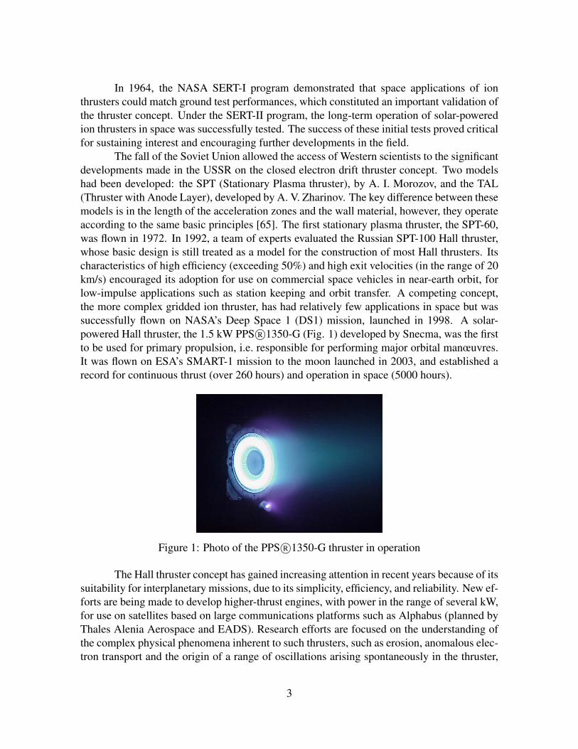
1 Photo of the PPS R©1350-G thruster in operation . . . . . . . . . . . . . . . . 32 Side view of the Hall thruster structure . . . . . . . . . . . . . . . . . . . . . 43 Characteristic magnetic and electric field distributions in a Hall thruster . . . 6
1.1 Scattering of an incident plane wave by particles . . . . . . . . . . . . . . . . 161.2 Distribution of electrons for a large scattered signal . . . . . . . . . . . . . . 181.3 Local oscillator and primary beams as used in heterodyne detection. The
beams intersect and create a common volume (light blue) centred in the re-gion of interest. . . . . . . . . . . . . . . . . . . . . . . . . . . . . . . . . . 19
1.4 30 kHz frequency peaks. In red - plasma signal, in black - photonic noise.The y-axis is in arbitrary units . . . . . . . . . . . . . . . . . . . . . . . . . 24
2.1 Configuration of optical bench elements on PRAXIS-I . . . . . . . . . . . . 272.2 Configuration of bench and external chassis around thruster vacuum vessel . . 312.3 Configuration of off-bench optical components on PRAXIS-I . . . . . . . . . 312.4 Setup of PRAXIS-I electronics . . . . . . . . . . . . . . . . . . . . . . . . . 332.5 Vacuum vessel at PIVOINE ground test facility with optical bench PRAXIS-I 352.6 . . . . . . . . . . . . . . . . . . . . . . . . . . . . . . . . . . . . . . . . . 362.7 Translator-rotator: rotation of primary about local oscillator beam . . . . . . 372.8 Virtual focus for establishing convergence in front of thruster exit . . . . . . 37
3.1 Coordinate system and placement of beams in front of thruster . . . . . . . . 403.2 . . . . . . . . . . . . . . . . . . . . . . . . . . . . . . . . . . . . . . . . . 433.3 Spectral densities obtained for different records for ~k oriented parallel to the
~E × ~B direction. A scattered signal near 5 MHz (blue line) is clearly visible.A lower-intensity peak, symmetric in frequency, is also visible. The photonicnoise spectrum (in red) and the PL + LO spectra (in green) superpose. Thebackground noise is in black. The peaks apparent around 0 MHz and -20MHz constitute stray signals. The observation wave number is 9630 rad/m. . 44
3.4 Spectral densities obtained for different records for ~k oriented parallel to ~E.The presence of a broad, high frequency scattered signal around 20 MHz(blue line) is clear. The peaks apparent around 0 MHz and -20 MHz constitutestray signals. The observation wave number is 6520 rad/m. . . . . . . . . . . 45
viii

3.5 The dynamic form factor of the ~E× ~B mode, corresponding to the data shownin Fig. 3.3, obtained after signal normalization . . . . . . . . . . . . . . . . . 47
3.6 Definition of frequency error ∆f . The Gaussian fit to the experimental dy-namic form factor is in blue. . . . . . . . . . . . . . . . . . . . . . . . . . . 49
3.7 Dispersion relations for the ~E × ~B mode. Dispersion relations for the posi-tive frequency peak, for identical experimental conditions but different align-ments, are in blue. The dispersion relation for a negative frequency peak isshown in red (absolute values). . . . . . . . . . . . . . . . . . . . . . . . . . 50
3.8 Dispersion relations for the ~E × ~B mode at different flow rates (in blue - 20mg/s, in red - 6 mg/s) . . . . . . . . . . . . . . . . . . . . . . . . . . . . . . 51
3.9 Dispersion relation for the axially-propagating mode . . . . . . . . . . . . . 513.10 Peak half-widths for the ~E × ~B mode as a function of wave number . . . . . 533.11 Lorentzian and Gaussian fits to the ~E × ~B mode normalized spectrum . . . . 543.12 Exponential variation of form factor S(~k) with wave number for the ~E × ~B
mode. The positive frequency peak data is in blue, the negative frequencypeak in red . . . . . . . . . . . . . . . . . . . . . . . . . . . . . . . . . . . . 55
3.13 Reference for azimuthal positions on thruster (referred to as clock hours).The thruster plume is directed out of the page . . . . . . . . . . . . . . . . . 56
3.14 Frequency variation with axial distance from the thruster exit plane for the~E × ~B mode . . . . . . . . . . . . . . . . . . . . . . . . . . . . . . . . . . 57
3.15 Frequency variation with axial distance from the thruster exit plane for theaxial mode . . . . . . . . . . . . . . . . . . . . . . . . . . . . . . . . . . . . 58
3.16 Form factor variation with axial distance from the thruster exit plane for the~E × ~B mode . . . . . . . . . . . . . . . . . . . . . . . . . . . . . . . . . . 59
3.17 Form factor variation with axial distance from the thruster exit plane for theaxial mode . . . . . . . . . . . . . . . . . . . . . . . . . . . . . . . . . . . . 60
3.18 Reference frame showing the ~E × ~B mode propagation . . . . . . . . . . . . 613.19 Frequency (Hz) as a function of ky and kx for the ~E × ~B mode . . . . . . . . 673.20 Growth rate (Hz) as a function of ky and kx for the ~E × ~B mode . . . . . . . 673.21 Frequency as a function of ky, for fixed kx = 0. . . . . . . . . . . . . . . . . 683.22 Growth rate as a function of ky, for fixed kx = 0. . . . . . . . . . . . . . . . . 683.23 Characteristic lobe frequencies as a function of ky, for kx = 0. . . . . . . . . . 693.24 Characteristic growth rates as a function of ky, for kx = 0. . . . . . . . . . . . 70
4.1 Configuration of optical bench elements on PRAXIS-II . . . . . . . . . . . . 784.2 . . . . . . . . . . . . . . . . . . . . . . . . . . . . . . . . . . . . . . . . . 794.3 Schematic of optical bench setup for determination of heterodyning efficiency 834.4 Orientation of ~k for calibration using an acoustic wave. The acoustic wave
vector is denoted by ~ka, the observation wave vector by ~k . . . . . . . . . . . 84
ix

5.1 Error in positioning of the measurement volume resulting from an imperfectsuperposition of the primary and local oscillator beams in the plane xOy. (a)shows the situation in the xOy plane and (b) the yOz plane, for an exagger-ated superposition error . . . . . . . . . . . . . . . . . . . . . . . . . . . . . 88
5.2 Positive (in blue) and negative (in red) frequency peak intensities as a func-tion of the beam intersection position along z . . . . . . . . . . . . . . . . . 89
5.3 Schematic of the observation volume (in light and dark grey) for two posi-tions of the beam intersection centre along z. ~r+ and ~r− are coincident withthe centre of the thruster channel on the 09h00 and 03h00 sides respectively;~r0 is the position of the observation volume center . . . . . . . . . . . . . . . 90
5.4 . . . . . . . . . . . . . . . . . . . . . . . . . . . . . . . . . . . . . . . . . 915.5 Comparison of fits to the intensity data when the mixed fit (full lines) and
Gaussian fit (dotted lines) are applied to the positive frequency peaks (inblue) and the negative frequency peaks (in red) . . . . . . . . . . . . . . . . 93
5.6 Variation of electron cyclotron drift length lce with radial position (left) anda schematic of wavefront deformation in the direction of propagation (right) . 95
6.1 Dispersion relation for the ~E × ~B mode, for an experiment featuring theminimum wave number . . . . . . . . . . . . . . . . . . . . . . . . . . . . . 99
6.2 Form factor variation with wave number, for an experiment featuring the min-imum wave number . . . . . . . . . . . . . . . . . . . . . . . . . . . . . . . 99
6.3 Poloidal coordinate system for the examination of the kθ and kx componentsof the wave vector when the laser beam crosses the thruster axis along z1; (a)shows a side view of the thruster with the reference angle α, which is varied,(b) shows the orientation of the wave vector components as viewed from thethruster face . . . . . . . . . . . . . . . . . . . . . . . . . . . . . . . . . . . 100
6.4 Variation of form factor of the ~E × ~B mode with α in the (kx, kθ) plane. Thepositive frequency peak data is shown in blue, the negative frequency peakdata in red . . . . . . . . . . . . . . . . . . . . . . . . . . . . . . . . . . . . 101
6.5 Relation between device angular resolution σd and wave number resolution ∆k1026.6 Comparison of experimental angular extension of the ~E × ~B mode in the
(kx, kθ) plane for the positive frequency peak (in blue) to the natural angularextension resulting from the device resolution (dotted line) . . . . . . . . . . 103
6.7 Variation of form factor of the ~E × ~B mode with α in the (kx, kθ) plane. Thepositive frequency peak data is shown in blue, the negative frequency peakdata in red . . . . . . . . . . . . . . . . . . . . . . . . . . . . . . . . . . . . 103
6.8 Variation of form factor of the axial mode with α in the (kx, kθ) plane . . . . 1056.9 Variation of the frequency of the positive frequency peak with α in the (kx, kθ)
plane, for the ~E × ~B mode . . . . . . . . . . . . . . . . . . . . . . . . . . . 1066.10 Variation of frequency of the axial mode with α in the (kx, kθ) plane, with
two fits applied: a simple cosine law (in red), and a modified cosine law (inblue) . . . . . . . . . . . . . . . . . . . . . . . . . . . . . . . . . . . . . . . 107
x

6.11 Configuration for the measurement of ~k aligned along ~B; (a) shows a sideview for the variation of α, (b) shows the orientation in which ~k may bealigned parallel to ~B, corresponding to α = 90 . . . . . . . . . . . . . . . . 108
6.12 Variation in form factor of modes with α in the plane (kx, kr), for the observa-tion volume situated at the lower thruster channel (06h00). Points pertainingto the axial mode positive frequency peak are in blue; points pertaining to theaxial mode negative frequency peak are in red; points identified as the “cath-ode mode” are in black. A Gaussian curve (dotted line) is shown superposedon the axial mode positive frequency peak data . . . . . . . . . . . . . . . . 109
6.13 Variation in form factor of modes with α in the plane (kx, kr), for the observa-tion volume situated at the upper thruster channel (12h00). Points pertainingto the axial mode positive frequency peak are in blue; points pertaining tothe axial mode negative frequency peak are in red. The cathode mode is ab-sent. A Gaussian curve (dotted line) is shown superposed on the axial modepositive frequency peak data . . . . . . . . . . . . . . . . . . . . . . . . . . 110
6.14 Dynamic form factor versus frequency for the case in which axial and “cath-ode” modes coexist (α = 45), observation in the (kx, kr) plane . . . . . . . . 111
6.15 . . . . . . . . . . . . . . . . . . . . . . . . . . . . . . . . . . . . . . . . . 1126.16 Variation in frequency of modes with α in the plane (kx, kr), for the observa-
tion volume situated at the lower thruster channel (06h00). Points pertainingto the axial mode positive frequency peak are in blue; points pertaining tothe axial mode negative frequency peak are in red; points identified as the“cathode mode” are in black. A cosine fit (dotted line) is shown applied tothe axial mode positive and negative frequency peak data . . . . . . . . . . . 113
6.17 Variation in frequency of modes with α in the plane (kx, kr), for the observa-tion volume situated at the upper thruster channel (12h00). Points pertainingto the axial mode positive frequency peak are in blue; points pertaining to theaxial mode negative frequency peak are in red. A cosine fit (dotted line) isshown applied to the axial mode positive and negative frequency peak data . . 114
6.18 Variation of frequency of the axial mode with α in the (kx, kθ) plane, withtwo fits applied: a simple cosine law (in red), and a modified cosine law (inblue). The observation volume is at the upper thruster channel . . . . . . . . 114
6.19 Configuration for the variation of the kr component of the observation wavevector. Beams are positioned at a height h relative to the thruster axis asshown in the side view (a) and front view (b) . . . . . . . . . . . . . . . . . . 115
6.20 Variation of form factor of the ~E × ~B mode with β (positive frequency peak) 1166.21 Variation of form factor of the ~E × ~B mode with β (negative frequency peak) 1176.22 Configurations for kr (in blue), k (in black), Vd (in green) and Vp (in red) for
the observation of the positive and negative frequency peaks of the ~E× ~B mode1186.23 Variation of form factor of the axial mode with β (positive frequency peak) . 1186.24 Variation of frequency for the ~E × ~B mode with β (positive frequency peak) . 1196.25 Variation of frequency for the axial mode with β (positive frequency peak) . . 120
xi

6.26 Variation in form factor with α for the ~E× ~B mode (positive frequency peak),for different β values: β = -0.08 (in green), β = 0.08 (in red), and β = 0.24(in blue) . . . . . . . . . . . . . . . . . . . . . . . . . . . . . . . . . . . . . 121
6.27 Variation in frequency with α for the ~E× ~B mode (positive frequency peak),for different β values: β = -0.08 (in green), β = 0.08 (in red), and β = 0.24(in blue) . . . . . . . . . . . . . . . . . . . . . . . . . . . . . . . . . . . . . 122
6.28 Directionality of most intense ~E × ~B mode, with a wave vector denoted by~km. Collective scattering observations have shown that α = 90 + 10.6 and β= 4.58 . . . . . . . . . . . . . . . . . . . . . . . . . . . . . . . . . . . . . 123
6.29 . . . . . . . . . . . . . . . . . . . . . . . . . . . . . . . . . . . . . . . . . 1246.30 Directionality of most intense axial mode on-axis, with a wave vector denoted
by ~km. Collective scattering observations have shown that α = 8.22 on-axis . 1256.31 Near-orthogonal propagation directions of the main ~E × ~B and axial modes
in the (kx, kθ) plane. ~ka represents the axial wave vector, ~ke the wave vectorof the ~E × ~B mode . . . . . . . . . . . . . . . . . . . . . . . . . . . . . . . 126
7.1 Frequency (Hz) as a function of ky and kx, for kz = 470 rad/m and vthe/Vd =1.8 . . . . . . . . . . . . . . . . . . . . . . . . . . . . . . . . . . . . . . . . 130
7.2 Growth rate (Hz) as a function of ky and kx, for kz = 470 rad/m and vthe/Vd= 1.8 . . . . . . . . . . . . . . . . . . . . . . . . . . . . . . . . . . . . . . . 131
7.3 Frequency as a function of ky, for kx = 0, kz = 470 rad/m and vthe/Vd = 1.8 . 1327.4 Growth rate as a function of ky, for kx = 0, kz = 470 rad/m and vthe/Vd = 1.8 . 1327.5 Frequency as a function of ky and kx, for kz = 470 rad/m and vthe/Vd = 2.5 . . 1337.6 Growth rate as a function of ky and kx, for kz = 470 rad/m and vthe/Vd = 2.5 . 1337.7 Frequency as a function of ky, for kx = 0, kz = 470 rad/m and vthe/Vd = 2.5 . 1347.8 Growth rate as a function of ky, for kx = 0, kz = 470 rad/m and vthe/Vd = 2.5 . 1347.9 Frequency as a function of ky and kx, for kz = 1000 rad/m and vthe/Vd = 2.5 . 1357.10 Growth rate as a function of ky and kx, for kz = 1000 rad/m and vthe/Vd = 2.5 1357.11 Frequency as a function of ky, for kx = 0, kz = 1000 rad/m and vthe/Vd = 2.5 . 1367.12 Growth rate as a function of ky, for kx = 0, kz = 1000 rad/m and vthe/Vd = 2.5 1377.13 Frequency as a function of α, for k = 6400 rad/m . . . . . . . . . . . . . . . 1387.14 Growth rate as a function of α, for k = 6400 rad/m . . . . . . . . . . . . . . 1387.15 Frequency as a function of α, for k = 8800 rad/m . . . . . . . . . . . . . . . 1397.16 Growth rate as a function of α, for k = 8800 rad/m . . . . . . . . . . . . . . 1407.17 Frequency as a function of kz, for k = 6000 rad/m . . . . . . . . . . . . . . . 1407.18 Growth rate as a function of kz, for k = 6000 rad/m . . . . . . . . . . . . . . 1417.19 Frequency as a function of kz, for k = 8000 rad/m . . . . . . . . . . . . . . . 1427.20 Growth rate as a function of kz, for k = 8000 rad/m . . . . . . . . . . . . . . 142
8.1 Form factor at different flow rates for the ~E × ~B mode, for the positive fre-quency peak (in blue) and negative frequency peak (in red) . . . . . . . . . . 148
8.2 Form factor ratio of positive frequency peak to the negative frequency peakat different flow rates for the ~E × ~B mode . . . . . . . . . . . . . . . . . . . 149
xii
8.3 Frequency of the ~E × ~B mode with flow rate (positive frequency peak) . . . 1498.4 Form factor at different flow rates for the axial mode . . . . . . . . . . . . . 1508.5 Frequency of the axial mode with flow rate . . . . . . . . . . . . . . . . . . 1518.6 Form factor of the ~E × ~B mode with discharge voltage (positive frequency
peak) . . . . . . . . . . . . . . . . . . . . . . . . . . . . . . . . . . . . . . 1528.7 Frequency of the ~E× ~B mode with discharge voltage (positive frequency peak)1528.8 Dispersion relation of the ~E × ~B mode with the magnetic field directed radi-
ally outwards (positive frequency peak) . . . . . . . . . . . . . . . . . . . . 1538.9 Form factor of the ~E × ~B mode with the magnetic field directed radially
outwards (positive frequency peak) . . . . . . . . . . . . . . . . . . . . . . . 1548.10 Comparison of dispersion relations of the ~E × ~B mode (positive frequency
peak) for different magnetic field strengths: 10 A (in red), 17 A (in green),and 24 A (in blue) . . . . . . . . . . . . . . . . . . . . . . . . . . . . . . . . 155
8.11 Variation of form factor with wave number of the ~E × ~B mode (positivefrequency peak) for different magnetic field strengths: 10 A (in red), 17 A (ingreen), and 24 A (in blue) . . . . . . . . . . . . . . . . . . . . . . . . . . . . 156
8.12 Variation of peak frequency with coil current for the ~E× ~B mode at k = 4890rad/m (positive frequency peak) . . . . . . . . . . . . . . . . . . . . . . . . 157
8.13 Variation of form factor with coil current for the ~E × ~B mode at k = 4890rad/m (positive frequency peak) . . . . . . . . . . . . . . . . . . . . . . . . 158
8.14 Variation of frequency with coil current for the axial mode at k = 4150 rad/m 1598.15 Variation of form factor with coil current for the axial mode at k = 4150 rad/m 1608.16 Raw low frequency spectra illustrating plasma oscillations detected by the
circuit and by collective scattering. . . . . . . . . . . . . . . . . . . . . . . . 1628.17 Discharge current oscillations for a 0.5 ms duration (from a total acquisition
duration of 0.13 s) . . . . . . . . . . . . . . . . . . . . . . . . . . . . . . . . 1638.18 . . . . . . . . . . . . . . . . . . . . . . . . . . . . . . . . . . . . . . . . . 1658.19 Low frequency normalized spectra at different wave numbers, with α=90 . . 1668.20 Low frequency normalized spectra at different flow rates, with α=90 and k
= 5928 rad/m . . . . . . . . . . . . . . . . . . . . . . . . . . . . . . . . . . 1668.21 Low frequency normalized spectra at different flow rates, with α=0 . . . . . 1678.22 . . . . . . . . . . . . . . . . . . . . . . . . . . . . . . . . . . . . . . . . . 1688.23 Frequency variation with coil current for α = 90 and k = 4890 rad/m . . . . 1698.24 Form factor variation with coil current for α = 90 and k = 4890 rad/m. Form
factor values correspond to frequency peaks of Fig. 8.23 . . . . . . . . . . . 170
9.1 Slab geometry of Hall thruster (plasma indicated in grey). The uniform mag-netic field ~B0 is directed out of the plane of the page along z, with the uniformelectric field ~E0 parallel to x . . . . . . . . . . . . . . . . . . . . . . . . . . 172
xiii

9.2 Geometry of the Hall thruster. The wave vector ~k is shown with its projec-tions along all three axes; ~k⊥ is the projected wave vector in the xOy plane.The coordinates of the velocity of an electron in the lab reference frame, ~v,and in the particle reference frame moving at the drift velocity, ~u = ~v − ~Vd,are shown. The angle Ψ is formed between u⊥ and the x axis. The anglesα and β shown on the figure are consistent with the definitions used duringexperiments, and the geometry shown would correspond to observations of anegative frequency peak of the ~E × ~B mode (in the 03h00 thruster channelside) . . . . . . . . . . . . . . . . . . . . . . . . . . . . . . . . . . . . . . . 174
A.1 Setup for the measurement of laser beam profile . . . . . . . . . . . . . . . . 188A.2 Reconstitution of laser beam profile; the low noise of the profiles obtained is
notable . . . . . . . . . . . . . . . . . . . . . . . . . . . . . . . . . . . . . . 189A.3 Beam profile at 267 mm from lens (experimental points in blue, Gaussian fit
in red) . . . . . . . . . . . . . . . . . . . . . . . . . . . . . . . . . . . . . . 191A.4 Beam waists at different distances from the lens . . . . . . . . . . . . . . . . 191
xiv

xv

List of Tables
1 Summary of characteristic Isp values for main propulsion methods [27] . . . 2
1.1 Summary of main SPT-100 thruster characteristics . . . . . . . . . . . . . . 22
2.1 Summary of key beam waists on PRAXIS-I bench . . . . . . . . . . . . . . . 292.2 Summary of lens focal lengths used on PRAXIS-I . . . . . . . . . . . . . . . 302.3 Summary of key distances on PRAXIS-I . . . . . . . . . . . . . . . . . . . . 302.4 Summary of key distances on off-bench assembly. . . . . . . . . . . . . . . . 322.5 Summary of main PPSX000-ML thruster characteristics . . . . . . . . . . . 35
3.1 Thruster and plasma parameters . . . . . . . . . . . . . . . . . . . . . . . . 633.2 Characteristic plasma frequency and length scales . . . . . . . . . . . . . . . 64
4.1 Summary of key distances on PRAXIS-II . . . . . . . . . . . . . . . . . . . 774.2 Summary of lens focal lengths used on PRAXIS-II . . . . . . . . . . . . . . 784.3 Summary of key beam waists on PRAXIS-II bench . . . . . . . . . . . . . . 784.4 Summary of key differences between PRAXIS-I and PRAXIS-II . . . . . . . 80
xvi


Introduction
The final frontier“If we have learned one thing from the history of invention and discovery, it
is that, in the long run - and often in the short one - the most daring propheciesseem laughably conservative.”
- Arthur C. Clarke (1917-2008), The Exploration of Space, 1951
THE history of artificial satellites began with the launch of Sputnik-1, by the Soviet Unionin 1957. Since then, satellites have found a wide range of applications in telecommuni-
cations and space exploration. Commercial satellites are used today for relaying communi-cations to ships and planes, telephony and for television and radio broadcasting. Satellitesequipped with scientific instruments gather data on the solar system, providing measurementson the Earth’s atmosphere, solar wind, cosmic rays, and atmospheric conditions on otherplanets. Vital to our everyday life, satellites and probes have made it possible to exploreenvironments and worlds beyond our own.
The goals of any satellite mission must be balanced with considerations of missioncost and feasibility. Perhaps the most critical area of the design is the propulsion system.Various technologies exist and are under development, however, the basic limitation on theperformance of these techologies is imposed by Tsiolkovsky’s rocket equation,
m0 = m1 e∆v
Isp×g (1)
in which m0 is the initial mass (with fuel) of the vehicle, m1 the final mass of thevehicle, and ∆v a measure of the effort required to perform a manœuvre, such as orbitaltransfer. Isp is the specific impulse and g the acceleration due to gravity; ve, the fuel exitvelocity, is Isp × g.
The exhaust velocities accessible during chemical propulsion are limited by the chem-ical bond energy, whereas in electric propulsion, the acceleration of the propellant occursseparately from its production. The mass savings in electric propulsion can be considerablebecause of the higher exhaust velocities which are achievable. Table 1 presents a comparisonof Isp values of different thruster types which have been used in flight.
To illustrate the advantages of electric propulsion over chemical propulsion, we mayconsider two propellant systems, one chemical and another electric (Hall or ion thruster),
1

both of which require a ∆v of 10 km/s. We may assume that the final vehicle mass for bothcases will be the same. From Eq. 1, for an exhaust velocity of around 4 km/s in the case ofchemical propulsion, and an exhaust velocity of about 35 km/s in the case of ion propulsion,the resulting initial vehicle mass of the electric propulsion system is only 11% of that of thechemical propulsion system; this is without even having taken into account the mass savingson other equipment. For missions requiring a high ∆v, chemical propulsion is not feasiblebecause of the large fuel requirements.
Thruster Specific impulse (s)Chemical (monopropellant) 150-225
Chemical (bipropellant) 300-450Resistojet 300
Arcjet 500-600Ion thruster 2500-3600
Hall thrusters 1500-2000Pulsed plasma thrusters 850-1200
Table 1: Summary of characteristic Isp values for main propulsion methods [27]
Various other propulsion technologies such as nuclear propulsion exist and are beingdeveloped. Nuclear systems are massive and require precautions for materials storage. Otherconcerns, such as the melting temperatures of materials used for reactor cores, must be ad-dressed. However, such systems would deliver even larger exhaust velocities than electricpropulsion. Other intriguing options, such antimatter propulsion, could potentially offer ex-haust velocities a few orders of magnitude larger than chemical propulsion, but are not yetavailable.
Electric propulsion has attracted a great deal of industrial and academic interest overthe past few decades, as a propulsion technology well-suited to interplanetary missions.Closed electron drift thrusters are a widely-used form of electric propulsion and will be thesubject of this introduction.
The development of closed electron drift thrusters
Closed electron drift or Hall effect thrusters (HETs) refer to a class of thrusters inwhich the electron drift is confined to an azimuthally-circulating cloud at the thruster exit,through which ions are accelerated to provide thrust.
The first ideas for electrostatically accelerating particles for a propulsion system weredescribed by Robert H. Goddard in 1906. From the late 1940s to the 1960s, experimentswere carried out to determine the feasibility of ion propulsion by von Braun and Stuhlinger.In parallel, Cleaver, Shepherd and Spitzer performed studies demonstrating the feasibility ofusing nuclear energy to provide electric power to ion thrusters.
2
In 1964, the NASA SERT-I program demonstrated that space applications of ionthrusters could match ground test performances, which constituted an important validation ofthe thruster concept. Under the SERT-II program, the long-term operation of solar-poweredion thrusters in space was successfully tested. The success of these initial tests proved criticalfor sustaining interest and encouraging further developments in the field.
The fall of the Soviet Union allowed the access of Western scientists to the significantdevelopments made in the USSR on the closed electron drift thruster concept. Two modelshad been developed: the SPT (Stationary Plasma thruster), by A. I. Morozov, and the TAL(Thruster with Anode Layer), developed by A. V. Zharinov. The key difference between thesemodels is in the length of the acceleration zones and the wall material, however, they operateaccording to the same basic principles [65]. The first stationary plasma thruster, the SPT-60,was flown in 1972. In 1992, a team of experts evaluated the Russian SPT-100 Hall thruster,whose basic design is still treated as a model for the construction of most Hall thrusters. Itscharacteristics of high efficiency (exceeding 50%) and high exit velocities (in the range of 20km/s) encouraged its adoption for use on commercial space vehicles in near-earth orbit, forlow-impulse applications such as station keeping and orbit transfer. A competing concept,the more complex gridded ion thruster, has had relatively few applications in space but wassuccessfully flown on NASA’s Deep Space 1 (DS1) mission, launched in 1998. A solar-powered Hall thruster, the 1.5 kW PPS R©1350-G (Fig. 1) developed by Snecma, was the firstto be used for primary propulsion, i.e. responsible for performing major orbital manœuvres.It was flown on ESA’s SMART-1 mission to the moon launched in 2003, and established arecord for continuous thrust (over 260 hours) and operation in space (5000 hours).
Figure 1: Photo of the PPS R©1350-G thruster in operation
The Hall thruster concept has gained increasing attention in recent years because of itssuitability for interplanetary missions, due to its simplicity, efficiency, and reliability. New ef-forts are being made to develop higher-thrust engines, with power in the range of several kW,for use on satellites based on large communications platforms such as Alphabus (planned byThales Alenia Aerospace and EADS). Research efforts are focused on the understanding ofthe complex physical phenomena inherent to such thrusters, such as erosion, anomalous elec-tron transport and the origin of a range of oscillations arising spontaneously in the thruster,
3
all of which have implications on thruster efficiency and lifetime. Such efforts take the formof experimental measurements, theoretical analysis and numerical models.
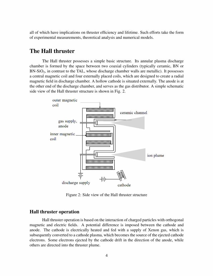
The Hall thrusterThe Hall thruster possesses a simple basic structure. Its annular plasma discharge
chamber is formed by the space between two coaxial cylinders (typically ceramic, BN orBN-SiO2, in contrast to the TAL, whose discharge chamber walls are metallic). It possessesa central magnetic coil and four externally placed coils, which are designed to create a radialmagnetic field in discharge chamber. A hollow cathode is situated externally. The anode is atthe other end of the discharge chamber, and serves as the gas distributor. A simple schematicside view of the Hall thruster structure is shown in Fig. 2.
Figure 2: Side view of the Hall thruster structure
Hall thruster operationHall thruster operation is based on the interaction of charged particles with orthogonal
magnetic and electric fields. A potential difference is imposed between the cathode andanode. The cathode is electrically heated and fed with a supply of Xenon gas, which issubsequently converted to a cathode plasma, which becomes the source of the ejected cathodeelectrons. Some electrons ejected by the cathode drift in the direction of the anode, whileothers are directed into the thruster plume.
4

The confinement of the electrons to a “closed drift” path near the thruster exit, wherethey circulate azimuthally, is strongly dependent on the magnetic field characteristics. Thechoice of magnetic field magnitude is designed to give the electrons a small Larmor radius(on the order of 1 mm), constraining them to wrap around the magnetic field lines and remainwithin the channel (which has a length of 2.5 cm and width of 1.5 cm in the case of the SPT-100). In contrast, the large Larmor radius of the ions (exceeding 1 m) allows them to exit thethruster channel with minimal deviation. The combination of the axial electric field ~E andradial magnetic field ~B produces an azimuthal electron drift of velocity Vd,
Vd =~E × ~B
B2≈ ExBr
(2)
The magnetic field increases to a maximum near the thruster exit and this config-uration helps stabilize the electric field distribution [54]. The field lines are also concave,resulting in higher magnetic field strength near the walls than in the centre of the channel;this configuration results in a “magnetic mirror effect”, first described in the thruster by Mo-rozov in 1968, which reduces electron-wall losses. This effect influences the electric potentialand consequently, the ion acceleration characteristics [38].
Xenon atoms flow into the discharge chamber via the anode and are ionized by theelectrons (with ionization rates around 90%), and the ions are accelerated out of the chamberby the electric field. Some electrons ejected by the cathode drift into the plume and neutralizethe ions. The majority of the ions are generated inside the thruster channel, in an ionizationzone, and accelerated near the exterior of the chamber in a region of high localized electricfield, where the electron mobility is small. One of the earliest experimental studies of theeffectiveness of the acceleration mechanism and the nature of thruster characteristics such asthe electron density distribution in the channel was provided by Bishaev and Kim [7].
The plasma potential is maximum at the anode (equal to the anode potential), wherethe magnetic field is weak and electron mobility high. It decreases towards the exit, approach-ing the cathode potential, while the magnetic field increases. This evolution in the magnitudeof the potential affects the energy distribution of the accelerated ions. The magnetic andelectric field distributions in a typical Hall thruster are shown qualitatively in Fig. 3.
Thrust is imparted to the vehicle via the magnetic field. The azimuthal electron driftand the radial magnetic field produce a force on the electrons equal to the electric field forceexerted on the ions (assuming that the number of electrons is equal to the number of ionsin the thruster channel). As will be seen in the next section, despite the relatively straight-forward mechanism of thrust generation, various phenomena with implications on efficiencyand lifetime occur in the Hall thruster.
An overview of Hall thruster phenomenaThe physical processes which take place in the Hall thruster are complex, and a num-
ber of the most important processes are described below.
5
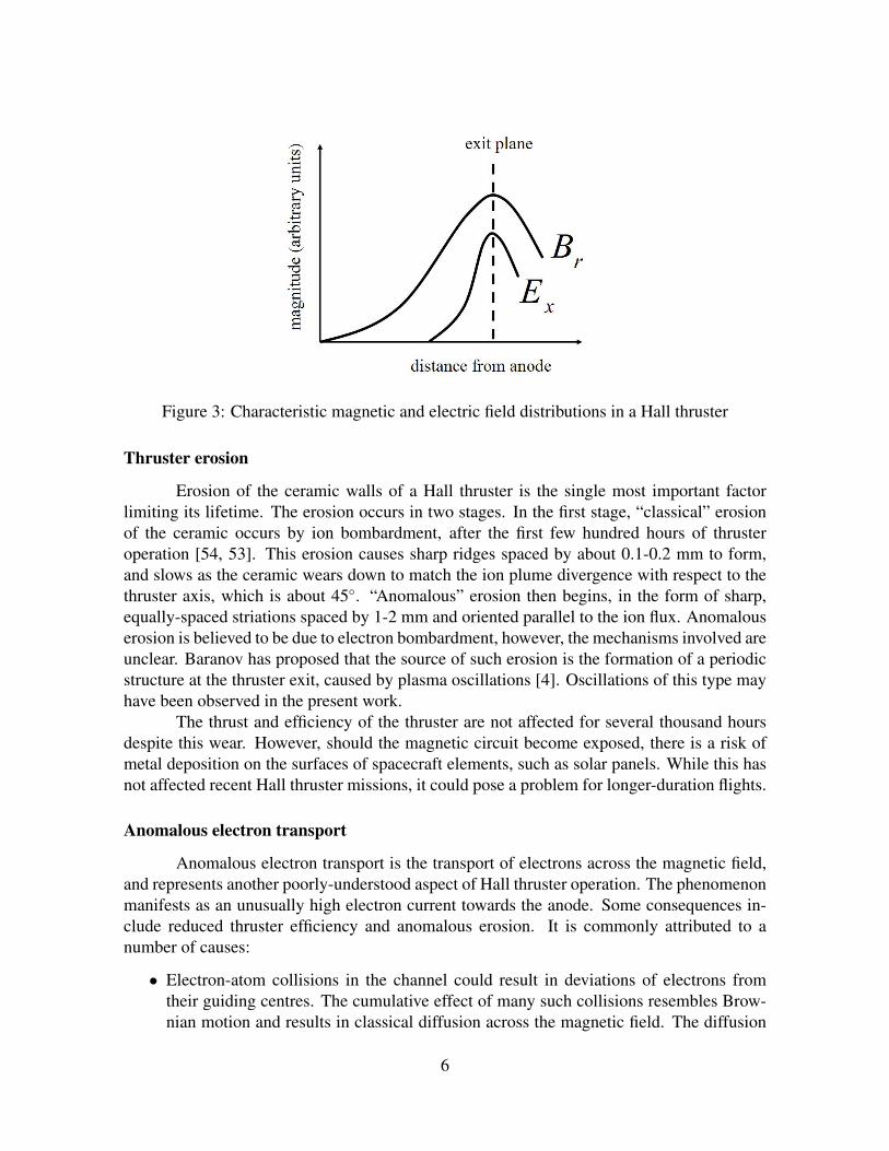
Figure 3: Characteristic magnetic and electric field distributions in a Hall thruster
Thruster erosion
Erosion of the ceramic walls of a Hall thruster is the single most important factorlimiting its lifetime. The erosion occurs in two stages. In the first stage, “classical” erosionof the ceramic occurs by ion bombardment, after the first few hundred hours of thrusteroperation [54, 53]. This erosion causes sharp ridges spaced by about 0.1-0.2 mm to form,and slows as the ceramic wears down to match the ion plume divergence with respect to thethruster axis, which is about 45. “Anomalous” erosion then begins, in the form of sharp,equally-spaced striations spaced by 1-2 mm and oriented parallel to the ion flux. Anomalouserosion is believed to be due to electron bombardment, however, the mechanisms involved areunclear. Baranov has proposed that the source of such erosion is the formation of a periodicstructure at the thruster exit, caused by plasma oscillations [4]. Oscillations of this type mayhave been observed in the present work.
The thrust and efficiency of the thruster are not affected for several thousand hoursdespite this wear. However, should the magnetic circuit become exposed, there is a risk ofmetal deposition on the surfaces of spacecraft elements, such as solar panels. While this hasnot affected recent Hall thruster missions, it could pose a problem for longer-duration flights.
Anomalous electron transport
Anomalous electron transport is the transport of electrons across the magnetic field,and represents another poorly-understood aspect of Hall thruster operation. The phenomenonmanifests as an unusually high electron current towards the anode. Some consequences in-clude reduced thruster efficiency and anomalous erosion. It is commonly attributed to anumber of causes:
• Electron-atom collisions in the channel could result in deviations of electrons fromtheir guiding centres. The cumulative effect of many such collisions resembles Brow-nian motion and results in classical diffusion across the magnetic field. The diffusion
6
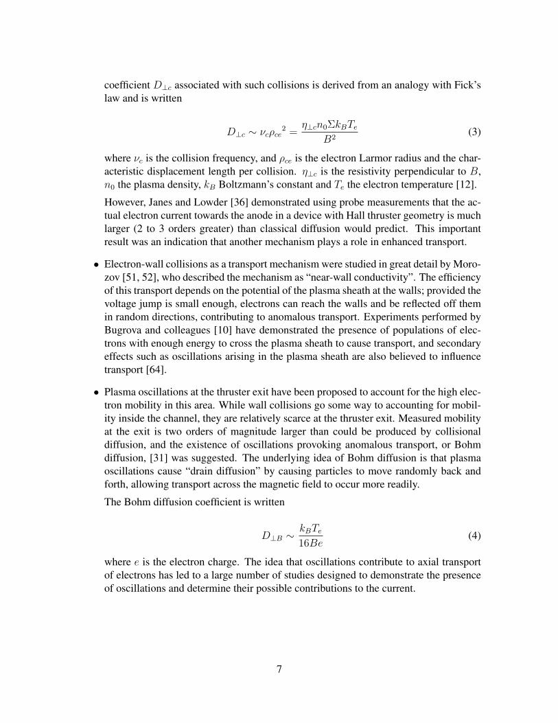
coefficient D⊥c associated with such collisions is derived from an analogy with Fick’slaw and is written
D⊥c ∼ νcρce2 =
η⊥cn0ΣkBTeB2
(3)
where νc is the collision frequency, and ρce is the electron Larmor radius and the char-acteristic displacement length per collision. η⊥c is the resistivity perpendicular to B,n0 the plasma density, kB Boltzmann’s constant and Te the electron temperature [12].
However, Janes and Lowder [36] demonstrated using probe measurements that the ac-tual electron current towards the anode in a device with Hall thruster geometry is muchlarger (2 to 3 orders greater) than classical diffusion would predict. This importantresult was an indication that another mechanism plays a role in enhanced transport.
• Electron-wall collisions as a transport mechanism were studied in great detail by Moro-zov [51, 52], who described the mechanism as “near-wall conductivity”. The efficiencyof this transport depends on the potential of the plasma sheath at the walls; provided thevoltage jump is small enough, electrons can reach the walls and be reflected off themin random directions, contributing to anomalous transport. Experiments performed byBugrova and colleagues [10] have demonstrated the presence of populations of elec-trons with enough energy to cross the plasma sheath to cause transport, and secondaryeffects such as oscillations arising in the plasma sheath are also believed to influencetransport [64].
• Plasma oscillations at the thruster exit have been proposed to account for the high elec-tron mobility in this area. While wall collisions go some way to accounting for mobil-ity inside the channel, they are relatively scarce at the thruster exit. Measured mobilityat the exit is two orders of magnitude larger than could be produced by collisionaldiffusion, and the existence of oscillations provoking anomalous transport, or Bohmdiffusion, [31] was suggested. The underlying idea of Bohm diffusion is that plasmaoscillations cause “drain diffusion” by causing particles to move randomly back andforth, allowing transport across the magnetic field to occur more readily.
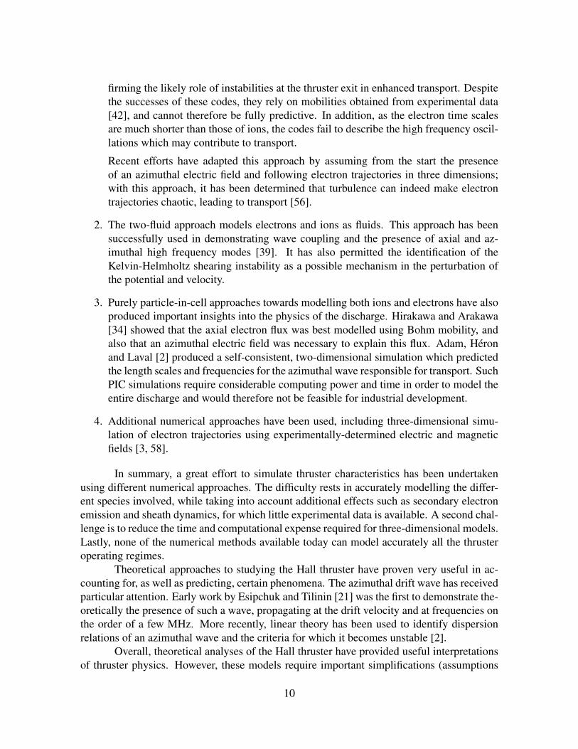
The Bohm diffusion coefficient is written
D⊥B ∼kBTe16Be
(4)
where e is the electron charge. The idea that oscillations contribute to axial transportof electrons has led to a large number of studies designed to demonstrate the presenceof oscillations and determine their possible contributions to the current.
7

Secondary electron emission
Electron bombardment of the thruster channel can liberate secondary electrons (“sec-ondary electron emission”, or SEE). Secondary electron emission from the wall material low-ers the sheath potential, increasing the proportion of electrons with sufficient energy to reachthe walls and contribute to axial conductivity. The contribution of SEE to backscattering andaxial electron conduction has been demonstrated in a number of numerical and experimen-tal studies ([19, 34, 23]), and the influence of the phenomenon on thruster discharge wasdiscussed in [25].
Spontaneous plasma oscillations
A wide range of oscillations, of different length scales and frequencies, arise in thethruster [14]. Some are generated by thruster processes such as ionization and gas depletion,while others arise because of the relative drift of the electron and ion species, or becauseof field and density non-uniformities. Their presence has significant consequences on thethruster discharge, stability of operation and lifetime, and is influenced by a wide varietyof parameters, including the magnetic field strength, discharge voltage and current, and gasflow rate. The general features and origins of some of the oscillations present are summarizedbelow.
1. Contour and ionization oscillations (frequencies 1-100 kHz): these oscillations are usu-ally related to the time required for an atom to travel the discharge channel and alsodepend on the discharge circuit. Near the channel exhaust, in the region of high elec-tric field and electron temperature, rapid ionization depletes the neutrals. The neutralfront retreats towards the anode, and consequently ionization and electron density atthe exit drop. The neutrals then flow back again towards the exit and the cycle is re-peated. These oscillations are of very high amplitude and result in large variations inthe discharge current and voltage. They are also termed as “breathing modes” and havebeen measured experimentally at frequencies of a few tens of kHz by several authors([8, 15, 46, 22]) and have been demonstrated numerically [32, 2].
2. Azimuthally-propagating oscillations (low frequency, 10-100 kHz)): low frequencyoscillations linked to the ionization process are seen to propagate in the direction ofthe azimuthal electron drift. The earliest identifications of the low frequency, rotating“spokes”, or density concentrations, were made by Janes and Lowder [36]. Esipchukand colleagues [20] also observed an isolated ionization wave of low frequency ro-tating azimuthally. The higher frequency oscillations in this category are due to non-uniformities in the density and magnetic field.
3. Azimuthally-propagating oscillations (high frequency, 1-100 MHz): these oscillationswere first observed experimentally in the Hall thruster geometry by Esipchuk andTilinin [21]. They performed a numerical analysis which revealed the presence ofthese oscillations in the plasma density, from frequencies of tens of kHz to several tens
8

of MHz, and measured what they termed “electron drift waves” at frequencies of 2-5MHz. Various subsequent experiments ([57, 50, 47, 60]) and numerical simulations([2, 39]) have confirmed the presence of azimuthal high frequency oscillations local-ized in the vicinity of the thruster exit.
The exact source of the high frequency oscillations in the azimuthal direction is notknown. Theoretical analysis by Litvak and Fisch [49] showed that these oscillationscould be manifestations of a Rayleigh instability and ascribed to axial gradients inmagnetic field, electron density and drift velocity. Other works [2] show that the largedrift velocity could be the source of the instability.
4. Ultra high frequency oscillations (several GHz): these oscillations are associated withelectron layers and flows of highly energetic electrons parallel and perpendicular to themagnetic field [65]. These oscillations have been identified in very few studies [6].
Background and context of this workThe present work is devoted to the identification and characterization of certain high
frequency modes at the thruster exit which are believed to play an important role in anomalouselectron transport.
As discussed earlier, there is an increasing need for the development of higher pow-ered Hall thrusters. However, due to the complexity of processes occurring in the thruster, ithas been necessary to rely on incremental improvements which must be tested at every stage.This development process is both costly and inefficient. For this reason, a vast research ef-fort is underway to better understand aspects of thruster physics, with the goal of developingpredictive models for its operation at different scales and improving thruster efficiency.
The numerical approach to modelling takes a number of forms.
1. Hybrid-PIC (particle-in-cell) approaches model the electrons as a fluid, and the ionsand neutrals as particles. Assumptions of quasineutrality require the use of trans-port equations to determine the electric field, otherwise the field may be deduced fromPoisson’s equation. Such models, whether one-dimensional (axial coordinate) or two-dimensional (radial and axial coordinates), have proven extremely useful for describ-ing physics of the ion and neutral time scales. Work by Fife [22] as well as Boeufand colleagues using hybrid-PIC models successfully demonstrated the presence of thethruster breathing mode [8, 5], as well as other oscillations of higher frequency [32].Various other features of the thruster, such as the relationship between the beam di-vergence and the oscillations, and the profiles of electric potential, plasma density andionization rate in the channel have also been calculated. Koo and Boyd have determinedparameters such as thrust and specific impulse using this modelling approach [41]. Ithas been applied not only to discharge characteristics, but to the study of features suchas thruster erosion after several thousand hours [40].
These methods require different electron mobilities inside and outside the thrusterchannel in order to account for the experimentally-measured discharge current, con-
9
firming the likely role of instabilities at the thruster exit in enhanced transport. Despitethe successes of these codes, they rely on mobilities obtained from experimental data[42], and cannot therefore be fully predictive. In addition, as the electron time scalesare much shorter than those of ions, the codes fail to describe the high frequency oscil-lations which may contribute to transport.
Recent efforts have adapted this approach by assuming from the start the presenceof an azimuthal electric field and following electron trajectories in three dimensions;with this approach, it has been determined that turbulence can indeed make electrontrajectories chaotic, leading to transport [56].
2. The two-fluid approach models electrons and ions as fluids. This approach has beensuccessfully used in demonstrating wave coupling and the presence of axial and az-imuthal high frequency modes [39]. It has also permitted the identification of theKelvin-Helmholtz shearing instability as a possible mechanism in the perturbation ofthe potential and velocity.
3. Purely particle-in-cell approaches towards modelling both ions and electrons have alsoproduced important insights into the physics of the discharge. Hirakawa and Arakawa[34] showed that the axial electron flux was best modelled using Bohm mobility, andalso that an azimuthal electric field was necessary to explain this flux. Adam, Heronand Laval [2] produced a self-consistent, two-dimensional simulation which predictedthe length scales and frequencies for the azimuthal wave responsible for transport. SuchPIC simulations require considerable computing power and time in order to model theentire discharge and would therefore not be feasible for industrial development.
4. Additional numerical approaches have been used, including three-dimensional simu-lation of electron trajectories using experimentally-determined electric and magneticfields [3, 58].
In summary, a great effort to simulate thruster characteristics has been undertakenusing different numerical approaches. The difficulty rests in accurately modelling the differ-ent species involved, while taking into account additional effects such as secondary electronemission and sheath dynamics, for which little experimental data is available. A second chal-lenge is to reduce the time and computational expense required for three-dimensional models.Lastly, none of the numerical methods available today can model accurately all the thrusteroperating regimes.
Theoretical approaches to studying the Hall thruster have proven very useful in ac-counting for, as well as predicting, certain phenomena. The azimuthal drift wave has receivedparticular attention. Early work by Esipchuk and Tilinin [21] was the first to demonstrate the-oretically the presence of such a wave, propagating at the drift velocity and at frequencies onthe order of a few MHz. More recently, linear theory has been used to identify dispersionrelations of an azimuthal wave and the criteria for which it becomes unstable [2].
Overall, theoretical analyses of the Hall thruster have provided useful interpretationsof thruster physics. However, these models require important simplifications (assumptions
10
on gradients, reduced dimensions, neglect of effects for which little experimental data isavailable) and can often only explain one particular aspect of thruster operation at a time.
The bulk of experimental measurements on the Hall thruster have focused on the useof probes and antennae (invasive and non-invasive).
Probe measurements have been used since the inception of the Hall thruster concept,first by Janes and Lowder to provide evidence of the role of the azimuthal density variations inanomalous electron diffusion. They have also been used to provide evidence of the existenceof electron populations of different energies and their contributions to near wall conductivity[10] and to study the acceleration and ionization zones [7]. Various other probe studieshave been able to measure ionization, transit time oscillations and azimuthal oscillations [22,45, 50]. Uncalibrated antenna measurements have also been used successfully to measurehigh frequency oscillations [60, 44, 57]. Certain other optical techniques such as opticalemission spectroscopy and laser induced fluorescence have been used to characterize ions inthe acceleration and ionisation zones, and are suited primarily for studying ion and neutralcharacteristics such as spatial velocity distributions.
This work draws its inspiration from the work of Adam et. al. in 2004 [2]. Thisnumerical study was the first self-consistent 2D PIC simulation to demonstrate that thrusterturbulence could account for anomalous transport. The most significant results from thiswork were the identification of:
• an azimuthal wave, of wavelength on the order of electron Larmor radius, near thethruster exit and possibly responsible for electron heating and transport,
• a vector component of the wave parallel to ~E,
• a wave frequency on the order of a few MHz
• a large-amplitude electric field fluctuation associated with the wave
These predictions have lacked experimental support, because no conventional experi-mental tools available at the time (or since) could measure fluctuations in the electric field atmillimetric length scales, inside the high temperature plasma. The smallest scales measurablevia antennae and probes are on the order of a centimetre [47]. A non-invasive collective lightscattering diagnostic has the potential of measuring the scales predicted to be significant intransport. This work was therefore dedicated to the construction and exploitation of one suchdiagnostic, in order to validate key theoretical and numerical predictions.
This work is organized in the following way.The important principles underlying collective light scattering and heterodyne detec-
tion are summarized in Chapter 1. An early collective scattering trial which helped to definethe requirements of the new collective light scattering bench, PRAXIS-I, is briefly presented.
Design details and experimental procedures for PRAXIS-I are presented in Chapter2. Chapter 3 deals with the range of experiments carried out using this bench and the gen-eral properties of the observed modes are described. Physical interpretations of the earlyresults are presented and a comparison of the results to the predictions of simple linear theoryperformed.
11
The second part of this work deals with a new series of experiments made possible byan upgrade of PRAXIS-I. The necessary improvements to PRAXIS-I and the newly-designedcollective scattering bench, PRAXIS-II, are presented in Chapter 4.
Experiments with the goal of localizing the modes and determining the significanceof the negative peak frequencies are described in Chapter 5. Chapter 6 focuses on the mea-surements of the directionality of the observed modes, concluding with a re-calculation ofthe true density fluctuation level.
Chapter 7 compares the experimental results to the solutions of the 3D theoreticaldispersion relation, describing key similarities and differences. A re-evaluation of a proposedelectron transport mechanism is performed, using the fluctuating field amplitude deducedfrom the density fluctuation characteristics.
Chapter 8 deals with the influence of varying thruster parameters on the characteristicsof the observed modes, with a focus on the effects of varying flow rate, magnetic field strengthand discharge voltage. Observations of low frequency oscillations are also described in thischapter.
Chapter 9 presents a new stability analysis of longitudinal plasma waves, such as areobserved experimentally, which takes into account the ion velocity and temperature.
The main text is concluded with a summary of the most important results and a de-scription of future work.
12

Part I
13

14

Chapter 1
Main concepts and preliminaries
Contents1.1 Collective light scattering as an experimental tool . . . . . . . . . . . . 15
1.1.1 Basic principles . . . . . . . . . . . . . . . . . . . . . . . . . . . . 16
1.2 Heterodyne detection . . . . . . . . . . . . . . . . . . . . . . . . . . . . 18
1.2.1 Necessity for heterodyne detection . . . . . . . . . . . . . . . . . . 18
1.2.2 Basic elements . . . . . . . . . . . . . . . . . . . . . . . . . . . . 19
1.2.3 Measured signal . . . . . . . . . . . . . . . . . . . . . . . . . . . 20
1.3 Collective scattering on the Hall thruster: first trial . . . . . . . . . . . 22
1.3.1 Results from experiment . . . . . . . . . . . . . . . . . . . . . . . 23
1.1 Collective light scattering as an experimental tool
COLLECTIVE light scattering (CLS) refers to an optical measurement technique wherebythe “collective” movements of a medium, due for example to the propagation of waves,
are studied using the elastic scattering of incident radiation by a non-uniform spatial distri-bution of particles. These particles are either atoms (in the case of Rayleigh scattering in aneutral gas), or electrons and ions (in the case of Thomson scattering in a plasma).
Light scattering is a technique which has been used to study the properties of dif-ferent media for several decades. It has been used for studying large molecules in solutionin chemistry, however, studies of characteristics such as thermal fluctuations at the level ofconstituent particles [55, 30] only became possible with the advent of lasers in the 1960’s.Light scattering techniques have been used to study turbulent liquids, via the seeding of theflow with particles [63, 28].
15

Figure 1.1: Scattering of an incident plane wave by particles
CLS is based on measurements of inhomogeneities inherent to the flow itself, ratherthan passive scalars which have been introduced into the flow. CLS has been applied to thestudy of gas flows [29, 9] and in magnetized plasmas to study features such as edge and coreturbulence and to determine scaling laws of density fluctuations [62, 16, 33]. The breadth ofapplications of this technique are proof of its versatility.
Collective light scattering possesses certain advantages over traditional techniques.Unlike many methods (such as probes and hot-wires), it does not induce a perturbation of themedium under investigation and the measurement volume may be situated virtually anywherein the flow, provided there are no optical obstructions to this. In the majority of thrusterstudies, probes are inserted into the ceramic wall, but cannot be used directly in the plumewithout damage due to the high temperature of the plasma. Using particles as passive scalarsin a flow is not always possible, and CLS circumvents this default. Exactly how this is donewill be explained in the next section.
1.1.1 Basic principlesAn electromagnetic wave incident on a charged particle will accelerate it, causing it
to re-emit another wave whose properties (frequency, wavenumber) depend on the incidentwave, and whose amplitude depends on the particle’s distance to the observer. Figure 1.1illustrates the scattering of an incident plane wave ~Ei(~r, t) by a group of particles situated at~rj . The incident wave at the position ~rj is of the form
~Ei(~r, t) = ~Ei0ei(~ki·~rj−ωit) (1.1)
The scattered e.m. wave is ~Es(~r, t). It is observed at an angle θ to the incident wave.In Fig. 1.1, the observation wave vector is constructed from the vector sum of the
scattering and incident wave vectors (~k = ~ks − ~ki). This is known as the Bragg relation.
16

Each electron may be considered as a dipole oscillating in the direction of the electricfield of the incident wave, acting as a point source for a spherical wave. With this approxi-mation, the total scattered field may be written as the summation of all the scattered waves,
~Es(~r′, t) = r0
∑j
eiki|~r′−~rj|~r′ − ~rj
e−i(~ki·~rj−ωit)~n′ ∧ (~n′ ∧ ~Ei0) (1.2)
where r0 is the Thomson scattering radius for free electrons,
r0 =1
4πε0
qe2
mec2(1.3)
Using a far-field approximation (i.e. where |~r′| |~rj| and |~r′| λi), the scatteredfield may be simplified to a superposition of plane wave fronts. With the aid of the reasonableassumption that the analysing wavelength 2π
kis much larger than the particle spacing, the total
scattered field from a volume Vs may be written as
~Es(~r′, t) = r0ei~ks·~r′
r′e−iωit ~Ei0
∫ ∫ ∫Vs
e−i~k·~rn(~r, t)d3~r (1.4)
Hence, the magnitude of the scattered field is proportional to the spatial Fourier trans-form of the density along ~k,
∫ ∫ ∫Vse−i
~k·~rn(~r, t)d3~r.
If the electrons are distributed randomly in space, the sum of their phases, Σe−i~k·~r,
and therefore the scattered signal magnitude, is small. If, instead, the electrons are distributedin regular manner, on planes perpendicular to ~k as in Fig. 1.2, such that
~k · (~rj+1 − ~rj) = 2π, (1.5)
the sum of phases is additive and the scattered signal is large. This is equivalentto saying that the projections of the positions ~rj in the direction ~nk are spaced a distanceλ0 = 2π
k, such that
~nk · (~rj+1 − ~rj) = λ0 (1.6)
In this way, a longitudinal wave propagating in a plasma may be identified via itsperiodic density concentrations. In a compressible, turbulent fluid medium, the scatteredsignal is obtained due to the presence of coherent structures in the flow.
The wave number k is a property of the medium under consideration, which maybe related to the incident wave number ki. ~ki and ~ks have the same magnitude, and k maytherefore be written
k = 2ki sin
(θ
2
)(1.7)
and λ0 as
17

λ0 =1
2 sin(θ2
)λi (1.8)
Hence the length scales of periodic density concentrations which may be measuredby collective scattering, for angles θ of typically few mrad, are several times the incidentwavelength.
Figure 1.2: Distribution of electrons for a large scattered signal
1.2 Heterodyne detection
1.2.1 Necessity for heterodyne detectionThe scattered field may be detected directly by a photodiode. The current produced is
proportional to the scattered field intensity on the surface, i.e. the Poynting vector flux acrossthe detector surface D. The detector is placed perpendicular to the direction of propagationof the wave, and the resulting power received on the detector, Ps, is written
Ps(t) =N
µ0c
∫ ∫D
∣∣∣ ~Es(~r′, t)∣∣∣2 d2~r′ (1.9)
using Eq. 1.4, this becomes
Ps(t) ∝∣∣∣∣∫ ∫ ∫
Vs
ei~k·~rn(~r′, t)d3~r
∣∣∣∣2 (1.10)
This form of Ps is inadequate, for two reasons:
• the scattered power is small and very difficult to detect,
• a complete description of the scattered field requires both the temporal phase infor-mation due to convection and the magnitude of the density fluctuation; the former ismissing from Eq. 1.10.
Heterodyne detection is therefore used to overcome these disadvantages by providinga signal of sufficient amplitude containing the phase information.
18
1.2.2 Basic elementsThe local oscillator
Heterodyne detection uses the combination of the scattered signal and a referencesignal, shifted in frequency but propagating in the same direction, to produce an interferenceterm measurable by the detector.
The reference signal is known as the local oscillator and has frequency ωLO, and thefrequency shift is ωm: ωLO = ωi + ωm.
ωm is much smaller than ωi, allowing the scattered radiation and the local oscillatorto remain in phase. ωm is chosen to be smaller than the passband of the detector (whichis around 1 GHz) and larger than the frequency range of the expected signal. The localoscillator amplitude used is as large as is permissible by the detector, in order to maximizethe amplitude of the interference term and thus the ease with which it may be detected.
The primary beam
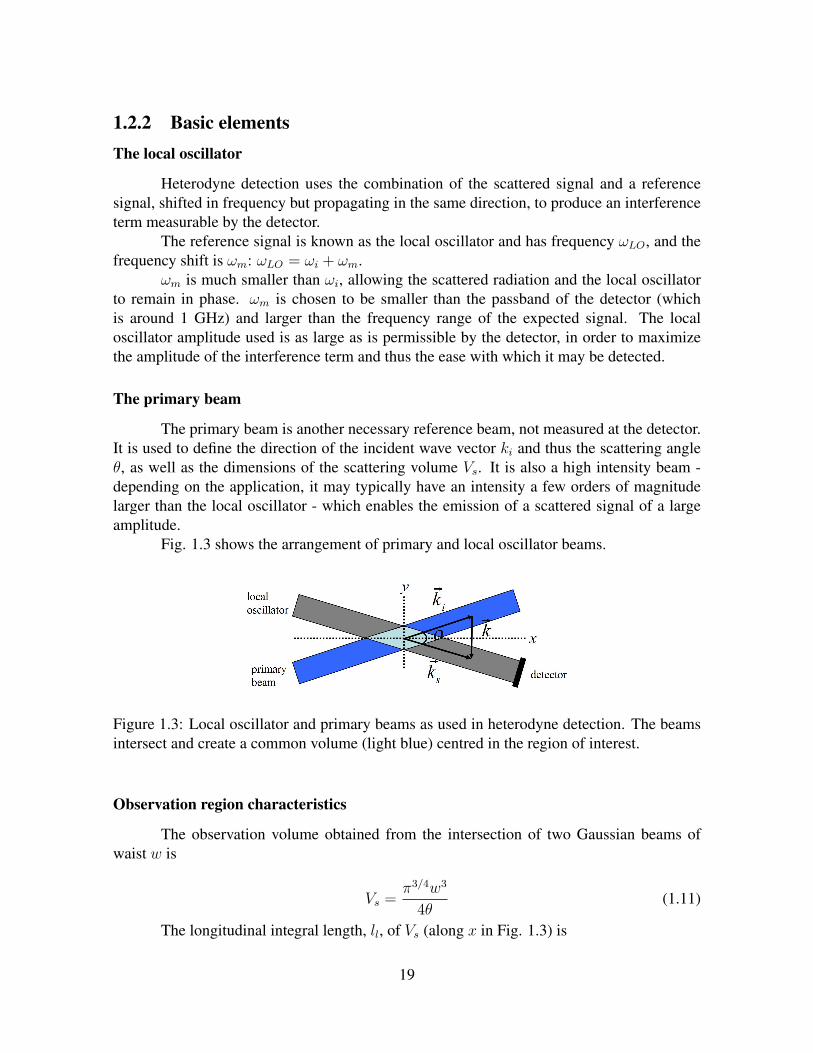
The primary beam is another necessary reference beam, not measured at the detector.It is used to define the direction of the incident wave vector ki and thus the scattering angleθ, as well as the dimensions of the scattering volume Vs. It is also a high intensity beam -depending on the application, it may typically have an intensity a few orders of magnitudelarger than the local oscillator - which enables the emission of a scattered signal of a largeamplitude.
Fig. 1.3 shows the arrangement of primary and local oscillator beams.
Figure 1.3: Local oscillator and primary beams as used in heterodyne detection. The beamsintersect and create a common volume (light blue) centred in the region of interest.
Observation region characteristics
The observation volume obtained from the intersection of two Gaussian beams ofwaist w is
Vs =π3/4w3
4θ(1.11)
The longitudinal integral length, ll, of Vs (along x in Fig. 1.3) is
19
ll =
√πw
θ(1.12)
while the transverse integral length, lt, is
lt =
√πw
2(1.13)
The longitudinal wave number resolution is given by
δkl =θ
w√
2(1.14)
while the transverse wave number resolution is
δkt =2√
2
w(1.15)
1.2.3 Measured signalInterference term
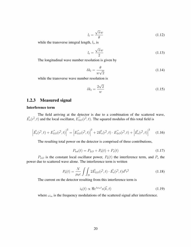
The field arriving at the detector is due to a combination of the scattered wave,~Es(~r′, t) and the local oscillator, ~ELO(~r′, t). The squared modulus of this total field is
∣∣∣ ~Es(~r′, t) + ~ELO(~r′, t)∣∣∣2 =
∣∣∣ ~ELO(~r′, t)∣∣∣2 + 2 ~Es(~r′, t) · ~ELO(~r′, t) +
∣∣∣ ~Es(~r′, t)∣∣∣2 (1.16)
The resulting total power on the detector is comprised of three contributions,
Ptot(t) = PLO + Pb(t) + Ps(t) (1.17)
PLO is the constant local oscillator power, Pb(t) the interference term, and Ps thepower due to scattered wave alone. The interference term is written
Pb(t) =N
µ0c
∫ ∫D
2 ~ELO(~r′, t) · ~Es(~r′, t)d2~r′ (1.18)
The current on the detector resulting from this interference term is
ib(t) ∝ <eiωmts(~k, t) (1.19)
where ωm is the frequency modulations of the scattered signal after interference.
20
Reconstitution of the scattered signal
The scattered signal is recovered in the following way:
• the current received by the photodiode is split into two parts: a continuous component(due to the constant local oscillator current), and a time-varying component (due to theinterference of the fields).
• the time-varying signal is amplified in a low noise amplifier
• the time-varying signal is then split into two parts for demodulation: the first part ismultiplied by a signal at frequency ωm, the second multiplied by another signal offrequency ωm but in quadrature with the first
• low-pass filters are applied to both parts of the signal to remove the term of frequency2ωm arising from the previous step
• both parts of the signal are amplified
The individual contributions of the signal (real and imaginary) are then combined as
s(~k, t) ∝ [xf (t) + iyf (t)] (1.20)
Eq. 1.20 contains all the time-varying characteristics of the scattered signal; the con-tinuous current value is retained for signal normalization.
Absolute measurement of density fluctuation
The measurable component of the scattered signal defined by the scattering volumeVs. Hence the signal received at the detector is not only a function of the density, but also thebeam profile U(r) [35], i.e.
s(~k, t) =
∫n(r′, t) U(~r)ei
~k·~rdr3 (1.21)
A Fourier transform is performed on this signal to give the spectral density.The mean square density fluctuation rate, assuming a Gaussian volume profile, is
〈n2〉n2
0
=1
4π3 |r20|λ2ls
2n02
~wηPP
∫ +∞
−∞
Ik(ω)
In
dω
2π(1.22)
where In is the photonic noise spectral density, defined as
In = e2ηPLO~w
(1.23)
n0 is the mean density of the measurement region. λ is the incident wavelength, ls thescattering length (much smaller than the dimension ll of the scattering volume), η the detectorefficiency, PP the power of the primary beam, and w the beam waist in the measurementregion. The term Ik(ω) is the spectral density of the scattered signal at a particular wavenumber k. A full development of this expression can be found in [29].
21
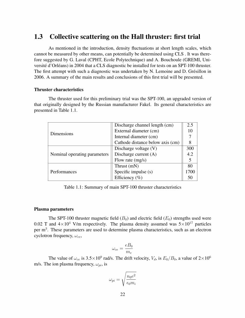
1.3 Collective scattering on the Hall thruster: first trialAs mentioned in the introduction, density fluctuations at short length scales, which
cannot be measured by other means, can potentially be determined using CLS . It was there-fore suggested by G. Laval (CPHT, Ecole Polytechnique) and A. Bouchoule (GREMI, Uni-versite d’Orleans) in 2004 that a CLS diagnostic be installed for tests on an SPT-100 thruster.The first attempt with such a diagnostic was undertaken by N. Lemoine and D. Gresillon in2006. A summary of the main results and conclusions of this first trial will be presented.
Thruster characteristics
The thruster used for this preliminary trial was the SPT-100, an upgraded version ofthat originally designed by the Russian manufacturer Fakel. Its general characteristics arepresented in Table 1.1.
Dimensions
Discharge channel length (cm) 2.5External diameter (cm) 10Internal diameter (cm) 7Cathode distance below axis (cm) 8
Nominal operating parametersDischarge voltage (V) 300Discharge current (A) 4.2Flow rate (mg/s) 5
PerformancesThrust (mN) 80Specific impulse (s) 1700Efficiency (%) 50
Table 1.1: Summary of main SPT-100 thruster characteristics
Plasma parameters
The SPT-100 thruster magnetic field (B0) and electric field (E0) strengths used were0.02 T and 4×10⁴ V/m respectively. The plasma density assumed was 5×10¹⁷ particlesper m3. These parameters are used to determine plasma characteristics, such as an electroncyclotron frequency, ωce,
ωce =eB0
me
The value of ωce is 3.5×10⁹ rad/s. The drift velocity, Vd, is E0/B0, a value of 2×10⁶
m/s. The ion plasma frequency, ωpi, is
ωpi =
√n0e2
ε0mi
22

ωpi is 8.2×10⁷ rad/s.
Expectations from theory and simulation
Linear theory predicts that the azimuthal drift instability arises only for certain dis-crete wave numbers (this will be discussed in more detail in Chapter 3). Simulations showthat the excited azimuthally-propagating instability is present within a wave number range of2600 - 13300 rad/m. The range of wavenumbers accessible during this trial is 3200 - 19200rad/m.
The predicted intensity of the fluctuations has been determined to be on the order of8×106, while the expected frequency dispersion is 107 Hz.
Expectations from existing optical bench
The collective scattering bench used was initially built for turbulent aerodynamicsexperiments performed twenty years ago [11]. It used a CO2, 10.6 µm-wavelength, 3 Wlaser. The beam waist in the convergence zone in front of the thruster was 5 mm.
The bench was installed on the SPT-100 Hall thruster with the local oscillator andprimary beams crossing in front of the thruster face at a distance of 10 mm. The thruster wasoperated at a flow rate of 6 mg/s. The beams, on leaving the bench, entered and exited thethruster vacuum vessel through ZnSe windows. The plasma-scattered radiation and the localoscillator beam were recovered by mirrors and sent to a detector on the bench.
The estimated signal-to-noise ratio was 2.4, which suggested that this optical benchwas already sufficiently sensitive for the measurement of the electron density fluctuations.Only minor modifications to the bench optics were made to adapt it to the experiment.
1.3.1 Results from experimentLow frequency signal
An intense signal at 30 kHz, up to 30 dB above the noise, was observed (Fig. 1.4).The frequency of this signal was independent of the wavenumber, however, its magnitudewas largest at small wavenumbers and at higher Xe flow rates and magnetic field values.
Surprisingly, this signal was present even with the detector closed, an indication thatthe signal measured was not a collective scattering signal, but represented instead a plasmaoscillation picked up by the electronics circuit.
Broadband high frequency signal
The expected broadband, high frequency signal was not immediately apparent on thespectra (with frequencies analyzed up to 10 MHz). Repeated aquisitions were made of theplasma signal to increase the number of points (which was limited by the oscilloscope at eachacquisition to 200,000) and averaged, and the noise signal treated in the same way. Averagingwas performed over 4×10⁷ samples. The net signal obtained after subtraction of the photonic
23
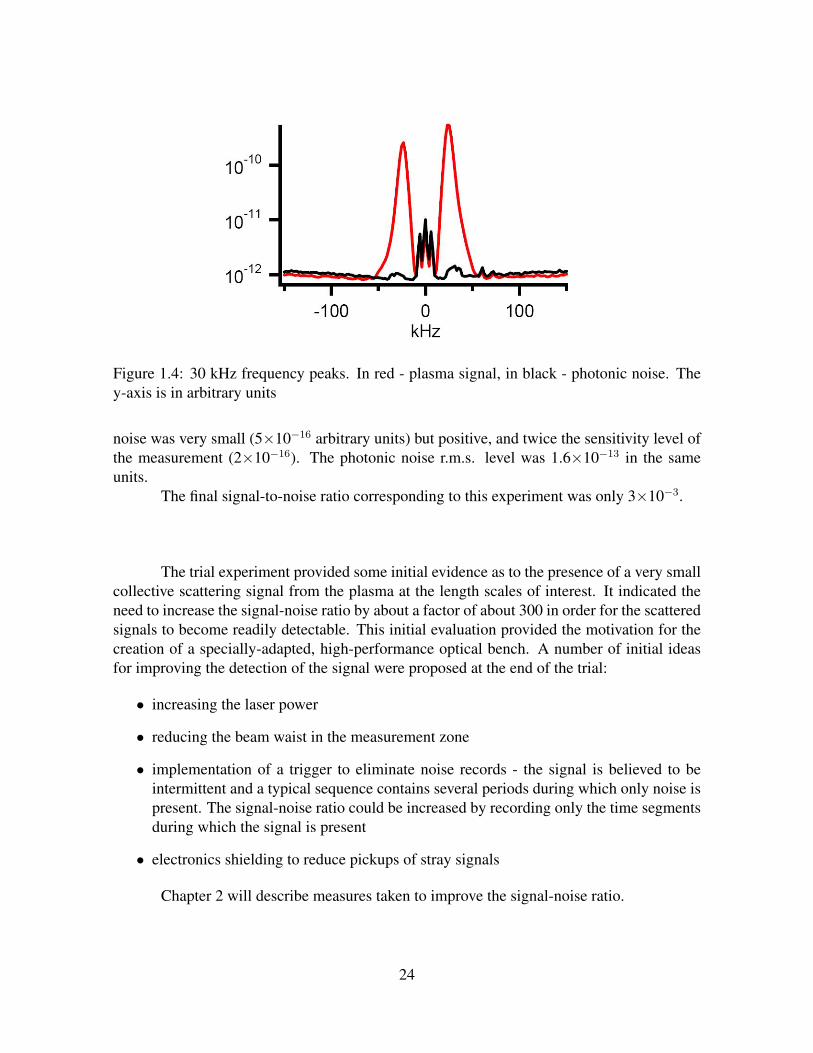
Figure 1.4: 30 kHz frequency peaks. In red - plasma signal, in black - photonic noise. They-axis is in arbitrary units
noise was very small (5×10⁻¹⁶ arbitrary units) but positive, and twice the sensitivity level ofthe measurement (2×10⁻¹⁶). The photonic noise r.m.s. level was 1.6×10⁻¹³ in the sameunits.
The final signal-to-noise ratio corresponding to this experiment was only 3×10⁻³.
The trial experiment provided some initial evidence as to the presence of a very smallcollective scattering signal from the plasma at the length scales of interest. It indicated theneed to increase the signal-noise ratio by about a factor of about 300 in order for the scatteredsignals to become readily detectable. This initial evaluation provided the motivation for thecreation of a specially-adapted, high-performance optical bench. A number of initial ideasfor improving the detection of the signal were proposed at the end of the trial:
• increasing the laser power
• reducing the beam waist in the measurement zone
• implementation of a trigger to eliminate noise records - the signal is believed to beintermittent and a typical sequence contains several periods during which only noise ispresent. The signal-noise ratio could be increased by recording only the time segmentsduring which the signal is present
• electronics shielding to reduce pickups of stray signals
Chapter 2 will describe measures taken to improve the signal-noise ratio.
24

Chapter 2
PRAXIS-I
Contents2.1 Main approaches for increasing signal-noise ratio . . . . . . . . . . . . 25
2.2 PRAXIS-I design . . . . . . . . . . . . . . . . . . . . . . . . . . . . . . . 26
2.2.1 On-bench assembly . . . . . . . . . . . . . . . . . . . . . . . . . . 26
2.2.2 Bench configuration . . . . . . . . . . . . . . . . . . . . . . . . . 28
2.2.3 Off-bench configuration . . . . . . . . . . . . . . . . . . . . . . . 30
2.2.4 Electronics and signal acquisition . . . . . . . . . . . . . . . . . . 32
2.2.5 Experimental facility and thruster . . . . . . . . . . . . . . . . . . 34
2.3 Experimental procedures . . . . . . . . . . . . . . . . . . . . . . . . . . 36
2.3.1 Beam alignment . . . . . . . . . . . . . . . . . . . . . . . . . . . 36
2.3.2 Calibration of wave vector . . . . . . . . . . . . . . . . . . . . . . 37
THE first trial revealed the necessity for dramatically increasing the signal-noise ratio. Anumber of basic design and construction decisions were made specifically to attain this
goal. A new optical bench, known as PRAXIS-I (PRopulsion Analysis eXperiments viaInfrared Scattering), was constructed. The design decisions for increasing the signal level aredescribed below.
2.1 Main approaches for increasing signal-noise ratio1. Beam power: The simplest method of increasing the signal-to-noise ratio involved
increasing the laser power. A GEM Select 50 W CoherentTM laser (42 W effectivepower) CO2 laser, wavelength 10.6 µm, replaced the 3 W laser used in the first trial.The expected gain in the scattered signal was a factor 14.
25
2. Optics: Losses at the mirror surfaces were reduced. The original bench used highly-polished steel mirrors, with a reflectivity of 95%, however, given the large number ofmirrors necessary to direct the beams, the final power losses of both primary and localoscillator beams were significant. Gold-coated copper mirrors (reflectivity 99%) anda large number of treated copper mirrors (reflectivity 99.8%) were therefore used onPRAXIS-I. The expected gain in signal over the previous bench was a factor larger than2.
3. Beam characteristics: The beam waist in the observation zone was reduced from theoriginal value of 5 mm to 2.5 mm, resulting in a factor 4 increase in the signal.
4. Acquisition: The 8-bit oscilloscope (acquisition rate 25MHz, 200,000 samples perchannel) used in the previous trial was replaced with a numerical acquisition modulefrom National Instruments, providing 14-bit resolution and an acquisition rate of up to100 MS/s (with 6.5 MS per channel being acquired). The advantages of this acquisitionmodule were three-fold:
• the high resolution allowed the weak signal to be more easily extracted from thebackground noise
• the larger number of samples allowed for more sophisticated post-acquisition pro-cessing
• the higher acquisition rate made it possible to record higher frequency signals
The final gain in signal was expected to exceed a factor of 5.
5. Detection: The detector from the previous bench (quantum efficiency of 0.3) was re-placed with another of quantum efficiency of 0.7, providing a gain in the signal levelof a factor 2.3
The final resulting gain in signal using PRAXIS-I, over the 2006 trial, was projectedto be at least a factor of 1250.
2.2 PRAXIS-I designThe design of PRAXIS-I is presented in this section.
2.2.1 On-bench assemblyThe bench design is shown in Fig. 2.1 and a description of certain critical components
of the optical bench are briefly presented below. In Fig. 2.1 the optical path of the primarybeam is shown in red, the local oscillator path in blue.
In the figure, M and MT are used to denote mirrors, with MT referring only to thelarge mirrors which are common to both primary and local oscillator beams. L represents the
26
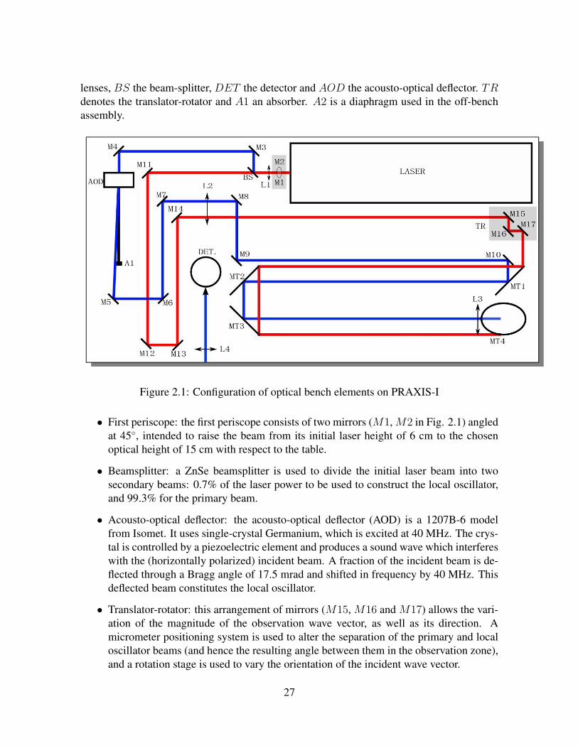
lenses, BS the beam-splitter, DET the detector and AOD the acousto-optical deflector. TRdenotes the translator-rotator and A1 an absorber. A2 is a diaphragm used in the off-benchassembly.
Figure 2.1: Configuration of optical bench elements on PRAXIS-I
• First periscope: the first periscope consists of two mirrors (M1, M2 in Fig. 2.1) angledat 45, intended to raise the beam from its initial laser height of 6 cm to the chosenoptical height of 15 cm with respect to the table.
• Beamsplitter: a ZnSe beamsplitter is used to divide the initial laser beam into twosecondary beams: 0.7% of the laser power to be used to construct the local oscillator,and 99.3% for the primary beam.
• Acousto-optical deflector: the acousto-optical deflector (AOD) is a 1207B-6 modelfrom Isomet. It uses single-crystal Germanium, which is excited at 40 MHz. The crys-tal is controlled by a piezoelectric element and produces a sound wave which interfereswith the (horizontally polarized) incident beam. A fraction of the incident beam is de-flected through a Bragg angle of 17.5 mrad and shifted in frequency by 40 MHz. Thisdeflected beam constitutes the local oscillator.
• Translator-rotator: this arrangement of mirrors (M15, M16 and M17) allows the vari-ation of the magnitude of the observation wave vector, as well as its direction. Amicrometer positioning system is used to alter the separation of the primary and localoscillator beams (and hence the resulting angle between them in the observation zone),and a rotation stage is used to vary the orientation of the incident wave vector.
27

• Second periscope: The beams are directed perpendicularly off the bench via MT4 inFig. 2.1, after which they are recovered by a second mirror and directed through thevacuum vessel window and across the thruster face.
According to the configuration shown, the initial laser beam encounters the firstperiscope, where its optical height is raised. It is then divided into two beams using a beam-splitter. The weaker beam (power 290 mW) is sent to the acousto-optical deflector, where alocal oscillator beam is created. The local oscillator beam is conducted using a series of mir-rors to M10, where together with the primary beam, it defines the orientation and magnitudeof the wave vector.
The primary beam travels undeviated across the beamsplitter and is directed to thetranslator-rotator. Together with the local oscillator it is conducted by a series of large mirrorsto the lens L3 and encounters the first periscope mirror MT4.
2.2.2 Bench configurationDue to the demanding nature of the experiment, care was taken to ensure beforehand
that each component performed as expected. Tests were performed to determine the limita-tions of different components.
The most critical of the characteristics is the M2 value of the laser beam. This value,described by the manufacturer as typically inferior to 1.1, was independently determined tobe 1.2 (the procedure is described in Appendix A). The bench was originally conceived for aperfect Gaussian beam with an M2 value of 1, and the elements were situated on the benchsuch as to respect restrictions on the beam size, e.g. the AOD has a window whose smallerdimension, hw, measures 6 mm. To avoid diffraction, a beam entering the window must havea waist w restricted to
w ≤ hw/4
The larger-than-expected divergence meant that this and other such conditions wereno longer respected. The bench was therefore redesigned to account for the divergence.
The position of the laser embedded waist was also independently determined andfactored into the calculation of the spacing of the bench elements.
The standard relations for Gaussian beam optics were used in determining the propa-gation of the beam and separation of the elements, with a modification due to the M2 value.As a function of the propagation distance z from the minimum beam waistw0, the beam waistis written
w(z) = w0
√1 +
(z
eR
)2
(2.1)
where the Rayleigh length, eR, is given by
eR =πw0
2
M2λ(2.2)
28

where λ is the laser wavelength. The Rayleigh length (the distance from the minimumbeam waist over which the electric field amplitude at the minimum waist is divided by 1/e)provides a measure of the beam expansion. The minimum beam waists and their correspond-ing distances on either side of a converging lens of focal length f are determined using therelations
di =f [do(do − f) + e2]
(do − f)2 + eR2(2.3)
wi =
√wo2f 2
(do − f)2 + eR2(2.4)
where di is the image distance from the lens, do the object distance from the lens, withe image waist and wo the object waist.
The beam waists are chosen according to two main criteria: (i) to prevent the beamfrom diffracting at critical locations such as the AOD, translator-rotator, and (ii) to fabricatethe desired 2.5 mm beam waist in the observation zone in front of the thruster. The mostimportant beam waists are listed in Table 2.1, in which Lw represents the embedded minimumlaser waist.
Elements Beam waist (mm) Rayleigh length (mm)Lw 1.09 291AOD 1.25 387TR 3.24 2587thruster axis 2.50 1544detector 0.069 1.176
Table 2.1: Summary of key beam waists on PRAXIS-I bench
The lens focal lengths and positions were chosen to produce the key beam waists.Wherever possible, the lenses and positions were chosen to be confocal for the sake of sim-plicity; the object distance do to the lens was set equal to the lens focal length. In this case,as is evident from Eq. 2.3, the image position di is also equivalent to the focal length and theratio wi to wo is the ratio of f to the Rayleigh length based on w0. The lens focal lengths areprovided in Table 2.2.
The resulting separations between the most important elements on the bench are sum-marized in Table 2.3.
The bench components are set up in a compact fashion on an aluminium-honeycomboptical table of dimensions 1.5 m by 0.75 m, equipped with rubber anti-vibration elementsbetween the table and its supporting legs.
29

Lens Focal length (mm)L1 381L2 1000L3 2000L4 190
Table 2.2: Summary of lens focal lengths used on PRAXIS-I
Elements Separation (mm)Lw - L1 535L1 - BS 50L1 - AOD 590AOD - L2 1000L2 - TR 1000TR - L3 2000
Table 2.3: Summary of key distances on PRAXIS-I
2.2.3 Off-bench configurationA system of mirrors and aluminium support structures allow the beams to be con-
ducted off the bench, across the plasma, and back to the bench. Fig. 2.2 shows the configu-ration of the bench and the external chassis on which the off-bench components (mirrors anddiaphragm) are mounted.
Fig. 2.3 is shows the beam trajectories after the beams leave the bench.The local oscillator and primary beams leave the bench together from MT4, after
which they are reflected by MT5 to intersect in front of the thruster exit plane at O. Thebeams are recovered on MT6 on the opposite side of the vacuum vessel and directed towardsan anodized aluminium diaphragm, A2. The local oscillator passes through a hole 2 cm indiameter in the centre of the diaphragm, while the primary is absorbed on the main plate,which has a diameter of 30 cm. The local oscillator (and the plasma-scattered radiation inthe same direction) is then directed by the mirrors M18, M19, M20 and M21 towards thebench. The lens L4 focuses the beam on the detector.
In the off-bench assembly, one beam waist is critical: the waist at O. The value of 2.5mm for this waist was chosen based on the resolution and minimum angle.
In the observation zone, a waist of 2.5 mm translates to a resolution δkt of 1130 rad/m.As will be discussed in more detail later, theoretical results indicate a possible saturation inthe mode amplitude in the range of 3000 - 4000 rad/m. One of the goals of this experimentwas to achieve minimum wave numbers on the same order. The smallest wave number whichcan be achieved experimentally must be a few times larger than δkt, and with the chosen
30
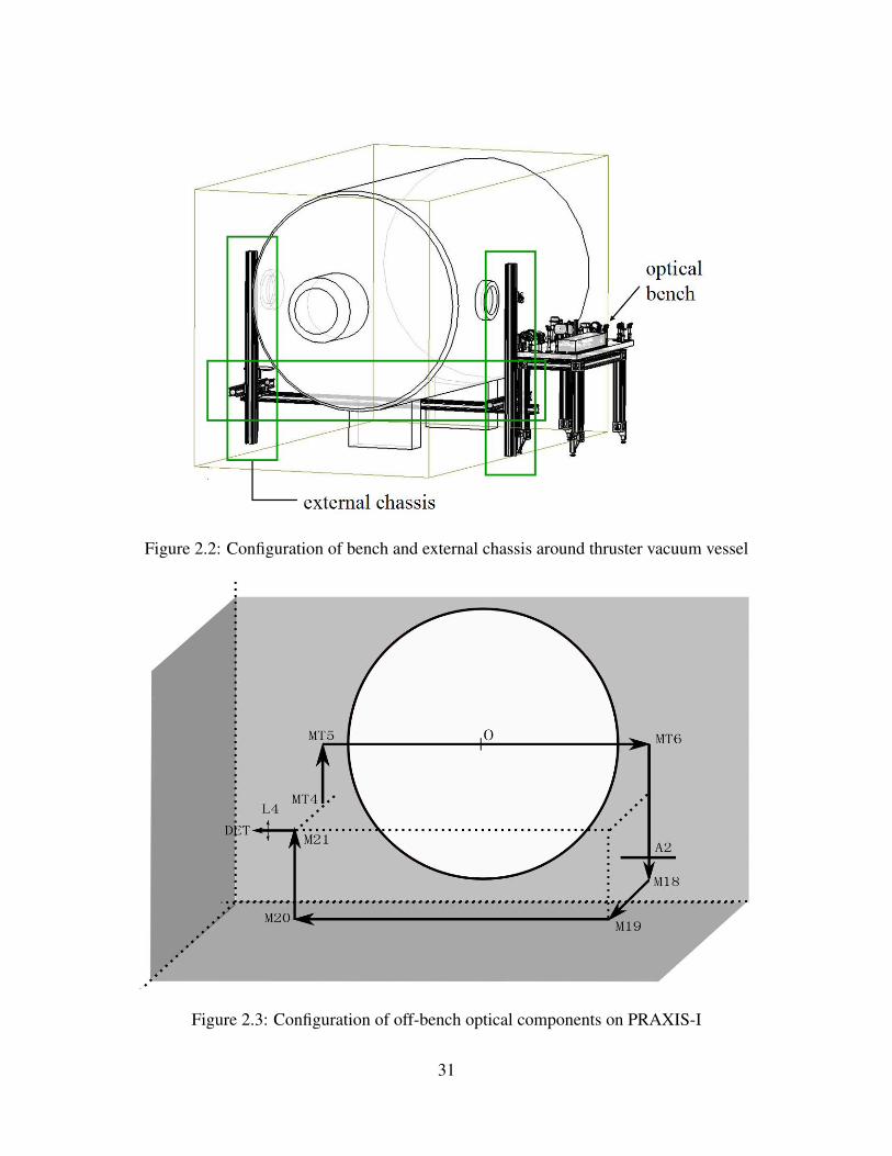
Figure 2.2: Configuration of bench and external chassis around thruster vacuum vessel
Figure 2.3: Configuration of off-bench optical components on PRAXIS-I
31
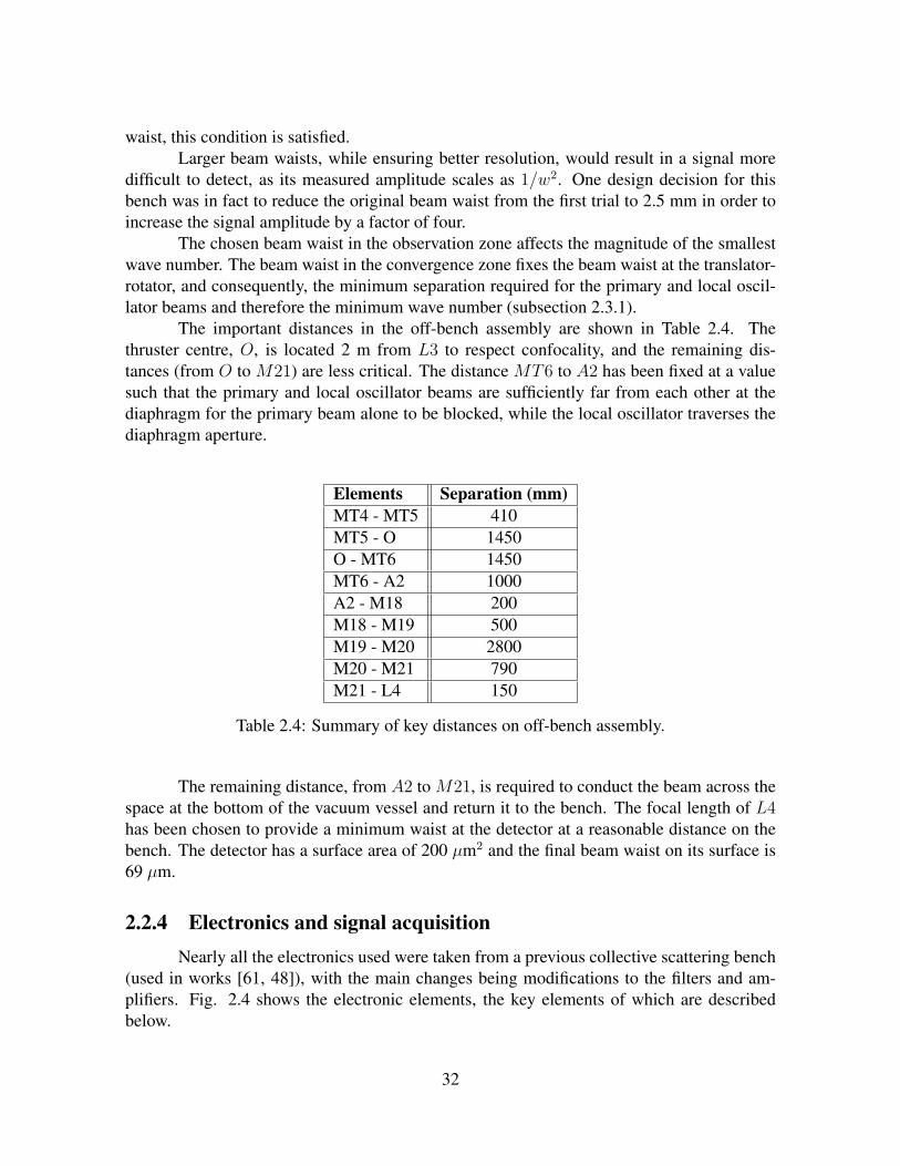
waist, this condition is satisfied.Larger beam waists, while ensuring better resolution, would result in a signal more
difficult to detect, as its measured amplitude scales as 1/w2. One design decision for thisbench was in fact to reduce the original beam waist from the first trial to 2.5 mm in order toincrease the signal amplitude by a factor of four.
The chosen beam waist in the observation zone affects the magnitude of the smallestwave number. The beam waist in the convergence zone fixes the beam waist at the translator-rotator, and consequently, the minimum separation required for the primary and local oscil-lator beams and therefore the minimum wave number (subsection 2.3.1).
The important distances in the off-bench assembly are shown in Table 2.4. Thethruster centre, O, is located 2 m from L3 to respect confocality, and the remaining dis-tances (from O to M21) are less critical. The distance MT6 to A2 has been fixed at a valuesuch that the primary and local oscillator beams are sufficiently far from each other at thediaphragm for the primary beam alone to be blocked, while the local oscillator traverses thediaphragm aperture.
Elements Separation (mm)MT4 - MT5 410MT5 - O 1450O - MT6 1450MT6 - A2 1000A2 - M18 200M18 - M19 500M19 - M20 2800M20 - M21 790M21 - L4 150
Table 2.4: Summary of key distances on off-bench assembly.
The remaining distance, from A2 to M21, is required to conduct the beam across thespace at the bottom of the vacuum vessel and return it to the bench. The focal length of L4has been chosen to provide a minimum waist at the detector at a reasonable distance on thebench. The detector has a surface area of 200 µm2 and the final beam waist on its surface is69 µm.
2.2.4 Electronics and signal acquisitionNearly all the electronics used were taken from a previous collective scattering bench
(used in works [61, 48]), with the main changes being modifications to the filters and am-plifiers. Fig. 2.4 shows the electronic elements, the key elements of which are describedbelow.
32
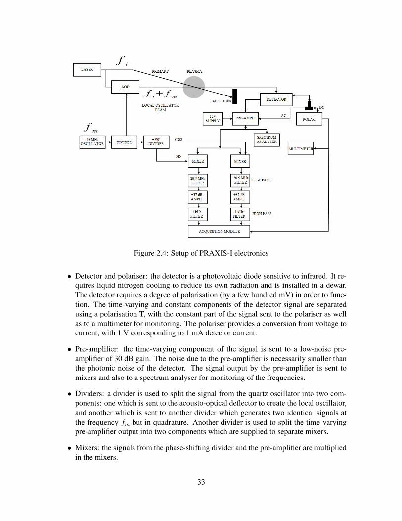
Figure 2.4: Setup of PRAXIS-I electronics
• Detector and polariser: the detector is a photovoltaic diode sensitive to infrared. It re-quires liquid nitrogen cooling to reduce its own radiation and is installed in a dewar.The detector requires a degree of polarisation (by a few hundred mV) in order to func-tion. The time-varying and constant components of the detector signal are separatedusing a polarisation T, with the constant part of the signal sent to the polariser as wellas to a multimeter for monitoring. The polariser provides a conversion from voltage tocurrent, with 1 V corresponding to 1 mA detector current.
• Pre-amplifier: the time-varying component of the signal is sent to a low-noise pre-amplifier of 30 dB gain. The noise due to the pre-amplifier is necessarily smaller thanthe photonic noise of the detector. The signal output by the pre-amplifier is sent tomixers and also to a spectrum analyser for monitoring of the frequencies.
• Dividers: a divider is used to split the signal from the quartz oscillator into two com-ponents: one which is sent to the acousto-optical deflector to create the local oscillator,and another which is sent to another divider which generates two identical signals atthe frequency fm but in quadrature. Another divider is used to split the time-varyingpre-amplifier output into two components which are supplied to separate mixers.
• Mixers: the signals from the phase-shifting divider and the pre-amplifier are multipliedin the mixers.
33
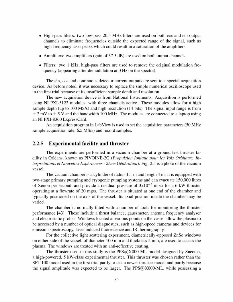
• High-pass filters: two low-pass 20.5 MHz filters are used on both cos and sin outputchannels to eliminate frequencies outside the expected range of the signal, such ashigh-frequency laser peaks which could result in a saturation of the amplifiers.
• Amplifiers: two amplifiers (gain of 37.5 dB) are used on both output channels
• Filters: two 1 kHz, high-pass filters are used to remove the original modulation fre-quency (appearing after demodulation at 0 Hz on the spectra).
The sin, cos and continuous detector current outputs are sent to a special acquisitiondevice. As before noted, it was necessary to replace the simple numerical oscilloscope usedin the first trial because of its insufficient sample depth and resolution.
The new acquisition device is from National Instruments. Acquisition is performedusing NI PXI-5122 modules, with three channels active. These modules allow for a highsample depth (up to 100 MS/s) and high resolution (14 bits). The signal input range is from± 2 mV to ± 5 V and the bandwidth 100 MHz. The modules are connected to a laptop usingan NI PXI-8360 ExpressCard.
An acquisition program in LabView is used to set the acquisition parameters (50 MHzsample acquisition rate, 6.5 MS/s) and record samples.
2.2.5 Experimental facility and thrusterThe experiments are performed in a vacuum chamber at a ground test thruster fa-
cility in Orleans, known as PIVOINE-2G (Propulsion Ionique pour les Vols Orbitaux: In-terpretations et Nouvelles Experiences - 2eme Generation). Fig. 2.5 is a photo of the vacuumvessel.
The vacuum chamber is a cylinder of radius 1.1 m and length 4 m. It is equipped withtwo-stage primary pumping and cryogenic pumping systems and can evacuate 150,000 litresof Xenon per second, and provide a residual pressure of 3x10⁻⁵ mbar for a 6 kW thrusteroperating at a flowrate of 20 mg/s. The thruster is situated at one end of the chamber andtypically positioned on the axis of the vessel. Its axial position inside the chamber may bevaried.
The chamber is normally fitted with a number of tools for monitoring the thrusterperformance [43]. These include a thrust balance, gaussmeter, antenna frequency analyserand electrostatic probes. Windows located at various points on the vessel allow the plasma tobe accessed by a number of optical diagnostics, such as high-speed cameras and devices foremission spectroscopy, laser-induced fluorescence and IR thermography.
For the collective light scattering experiment, diametrically-opposed ZnSe windowson either side of the vessel, of diameter 100 mm and thickness 5 mm, are used to access theplasma. The windows are treated with an anti-reflective coating.
The thruster used in this study is the PPS R©X000-ML model designed by Snecma,a high-powered, 5 kW-class experimental thruster. This thruster was chosen rather than theSPT-100 model used in the first trial partly to test a newer thruster model and partly becausethe signal amplitude was expected to be larger. The PPS R©X000-ML, while possessing a
34
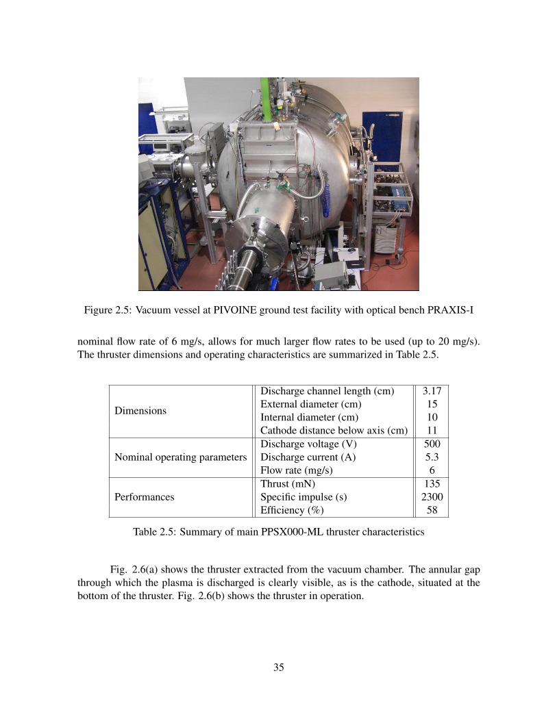
Figure 2.5: Vacuum vessel at PIVOINE ground test facility with optical bench PRAXIS-I
nominal flow rate of 6 mg/s, allows for much larger flow rates to be used (up to 20 mg/s).The thruster dimensions and operating characteristics are summarized in Table 2.5.
Dimensions
Discharge channel length (cm) 3.17External diameter (cm) 15Internal diameter (cm) 10Cathode distance below axis (cm) 11
Nominal operating parametersDischarge voltage (V) 500Discharge current (A) 5.3Flow rate (mg/s) 6
PerformancesThrust (mN) 135Specific impulse (s) 2300Efficiency (%) 58
Table 2.5: Summary of main PPSX000-ML thruster characteristics
Fig. 2.6(a) shows the thruster extracted from the vacuum chamber. The annular gapthrough which the plasma is discharged is clearly visible, as is the cathode, situated at thebottom of the thruster. Fig. 2.6(b) shows the thruster in operation.
35
(a) The PPS R©X000-ML thruster outside thevacuum chamber
(b) The PPS R©X000-ML thruster firing inthe vacuum chamber
Figure 2.6: The PPS R©X000-ML thruster
2.3 Experimental proceduresSome of the procedures followed for calibration and positioning of the beams are
presented briefly in this section.
2.3.1 Beam alignmentThe alignment of the beams is complicated by two factors: (i) the beams travel a very
long distance - from the locations where the primary and local oscillator are created, eachtravels a total distance of 6 m to the convergence zone in front of the thruster, and (ii) thevolume occupied by the vacuum vessel is inaccessible, and the positioning of the beams inthe front of the thruster cannot be directly viewed.
Care is taken to first assure alignment on the bench. In order to define the wavenumber, on rotation the primary must describe a circle of constant radius r about the localoscillator in the wv plane as shown in Fig. 2.7.
In Fig. 2.7, M17 rotates in the wv plane to change the scattering plane in which theobservation wave vector is situated; this is done using the rotator element (a goniometer).The distance between M16 and M17 is changed to alter the magnitude of the observationwave vector; this is done using the translator element (a micrometer vernier).
The radius must not change with the distance to the convergence zone. This is checkedby an iterative alignment procedure where the near-field and far-field beam positions arecorrected in small steps.
To ensure convergence, a “virtual” focus is created by redirecting the beams to a pointaway from the vacuum vessel, and checking the convergence there (Fig. 2.8). The redirection
36

Figure 2.7: Translator-rotator: rotation of primary about local oscillator beam
of the beams is done using a mirror installed temporarily afterMT4, identified asMR in Fig.2.8. The distance between L3 and the virtual focus plane is 2000 mm. If necessary, additionalslight adjustments are made to the orientations of the lenses M16, M17 and M10 such thatthe primary and local oscillator converge at the same point on the virtual focus plane. Oncethis is assured, MR is removed and the beams allowed to follow the usual trajectory towardsMT5.
Figure 2.8: Virtual focus for establishing convergence in front of thruster exit
Once the convergence has been checked, the beams are redirected across the vacuumvessel.
2.3.2 Calibration of wave vectorThe beam waists at the translator-rotator are imposed by the required beam waist in
front of the thruster. This in turn fixes a certain minimum separation distance, r0, betweenthe beams at the translator-rotator, which is four times the beam waist to avoid diffraction.
The separation distance fixes the angle between the beams in the convergence zone,which in mrad is
37
θ [mrad] = r [mm] /2 (2.5)
since the focal length of L3 is 2000 mm.The wave number k in rad/m is given by
k =2πθ
λ(2.6)
In the present bench configuration, the beam waists at the translator-rotator are 3.24mm; this translates to an expected minimum angle of 6.48 mrad between the beams in theconvergence zone, or a minimum wave number of 3841 rad/m.
The maximum wave number is fixed by the maximum separation allowed at L3 be-tween the beams, where the local oscillator is placed in the centre of the lens. Because ofrestrictions such as the dimensions of the lens holder, the maximum separation of the beamswithout diffraction is about 48 mm, corresponding to a maximum possible wave number of14226 rad/m.
The most important bench characteristics have been presented in this chapter. Theinitial ideas for improving the signal-noise ratio have been taken into account during theconception of PRAXIS-I. The beam trajectories on and off the bench have been carefullychosen and the desired beam waists imposed at the different locations. Unexpected problems,such as the large beam divergence, have been compensated for in the design.
The set of experiments carried out using PRAXIS-I are described in Chapter 3.
38

Chapter 3
Phase I experiments
Contents3.1 Signal acquisition and spectra details . . . . . . . . . . . . . . . . . . . 41
3.2 Evidence of high frequency modes . . . . . . . . . . . . . . . . . . . . . 42
3.3 Signal analysis techniques . . . . . . . . . . . . . . . . . . . . . . . . . . 45
3.3.1 Signal normalization . . . . . . . . . . . . . . . . . . . . . . . . . 45
3.3.2 Static form factor . . . . . . . . . . . . . . . . . . . . . . . . . . . 47
3.3.3 Characteristic frequency of a mode . . . . . . . . . . . . . . . . . 48
3.3.4 Error bars on wave number and frequency . . . . . . . . . . . . . . 48
3.4 Dispersion relations . . . . . . . . . . . . . . . . . . . . . . . . . . . . . 49
3.4.1 Dispersion relations for ~E × ~B mode . . . . . . . . . . . . . . . . 49
3.4.2 Dispersion relations for the axial mode . . . . . . . . . . . . . . . 50
3.5 Peak width of the ~E × ~B mode . . . . . . . . . . . . . . . . . . . . . . . 52
3.6 Energy distribution with length scale . . . . . . . . . . . . . . . . . . . 54
3.6.1 Form factor dependence on wave number for the ~E × ~B mode . . . 54
3.7 Frequency dependence on position along the thruster axis 0′x . . . . . . 57
3.7.1 Frequency dependence on axial position for the ~E × ~B mode . . . 57
3.7.2 Frequency dependence on axial position for the axial mode . . . . . 58
3.8 Form factor dependence on position along the thruster axis 0′x . . . . . 59
3.8.1 Form factor dependence on axial position for the ~E × ~B mode . . . 59
3.8.2 Form factor dependence on axial position for the axial mode . . . . 59
3.9 Total density fluctuation rate of the ~E × ~B mode . . . . . . . . . . . . . 60
3.10 Further interpretations and analysis . . . . . . . . . . . . . . . . . . . . 62
3.10.1 A hypothetical determination of the electron temperature . . . . . . 62
39
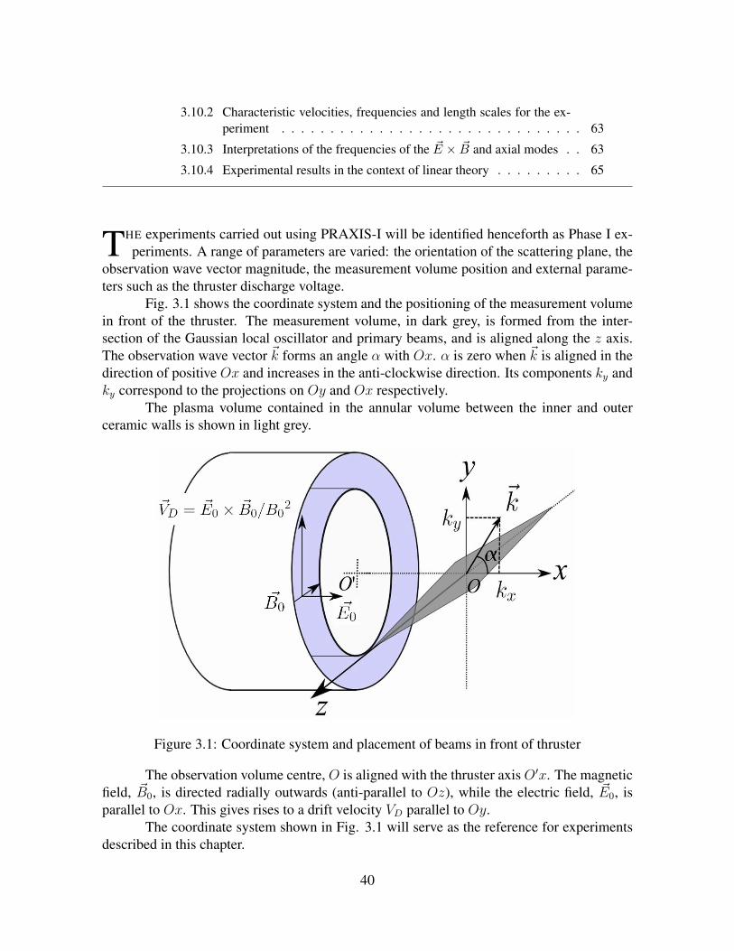
3.10.2 Characteristic velocities, frequencies and length scales for the ex-periment . . . . . . . . . . . . . . . . . . . . . . . . . . . . . . . 63
3.10.3 Interpretations of the frequencies of the ~E × ~B and axial modes . . 63
3.10.4 Experimental results in the context of linear theory . . . . . . . . . 65
THE experiments carried out using PRAXIS-I will be identified henceforth as Phase I ex-periments. A range of parameters are varied: the orientation of the scattering plane, the
observation wave vector magnitude, the measurement volume position and external parame-ters such as the thruster discharge voltage.
Fig. 3.1 shows the coordinate system and the positioning of the measurement volumein front of the thruster. The measurement volume, in dark grey, is formed from the inter-section of the Gaussian local oscillator and primary beams, and is aligned along the z axis.The observation wave vector ~k forms an angle α with Ox. α is zero when ~k is aligned in thedirection of positive Ox and increases in the anti-clockwise direction. Its components ky andky correspond to the projections on Oy and Ox respectively.
The plasma volume contained in the annular volume between the inner and outerceramic walls is shown in light grey.
Figure 3.1: Coordinate system and placement of beams in front of thruster
The observation volume centre, O is aligned with the thruster axis O′x. The magneticfield, ~B0, is directed radially outwards (anti-parallel to Oz), while the electric field, ~E0, isparallel to Ox. This gives rises to a drift velocity VD parallel to Oy.
The coordinate system shown in Fig. 3.1 will serve as the reference for experimentsdescribed in this chapter.
40

3.1 Signal acquisition and spectra detailsFor each acquisition, signals are recorded on three channels: cos, sin, and detector
current. The number of samples, N , was set at 6.5×10⁶. A high acquisition rate (50 MHz) ischosen to allow the resolution of high frequency oscillations in the signal. The total acquisi-tion duration is 0.13 s.
The spectral density of each signal acquisition requires a Fourier transform of thecomplex signal, written as
f(t) = XA+ iXB (3.1)
where XA represents the cos channel output, and XB the sin channel output, in mV.The discrete Fourier transform, F(ω), is determined in Matlab for the series f(t), of
length N , using the algorithm
F (ω) =N∑j=1
f(j)qN(j−1)(ω−1) (3.2)
where
qN = e(−2πi)/N (3.3)
As will be shown soon, four types of acquisitions are necessary for determining theabsolute scattered signal level. These are:
(a) Plasma + primary + local oscillator (to be referred to as PL+PB+LO): made with theplasma on, and the local oscillator and primary beams present. The corresponding signalis one which is expected to show evidence of a plasma fluctuation.
(b) Plasma + local oscillator (PL+LO): made with the plasma on and only the local oscillatorbeam present (the primary beam being blocked by an absorber on the bench). No plasma-scattered signal is expected to be present, unless stray radiation from the thruster currentpollutes the acquisition channels.
(c) Primary + local oscillator (PB+LO): made with the plasma off, but both primary andlocal oscillator beams present. This acquisition is used to determine the spectral densityof the photonic noise.
(d) Detector closed (D): made with the detector closed and the thruster running. This acqui-sition is used to determine the base electronic noise spectral density, due to thermal andamplifier noise.
The spectral density for each acquisition type is determined from the Fourier trans-form. The spectral density is calculated over a reduced time series of length n (such as 2001
1Use of a comparable 2n length for the slice, such as 256, had a negligible effect on the time required forthe calculation
41
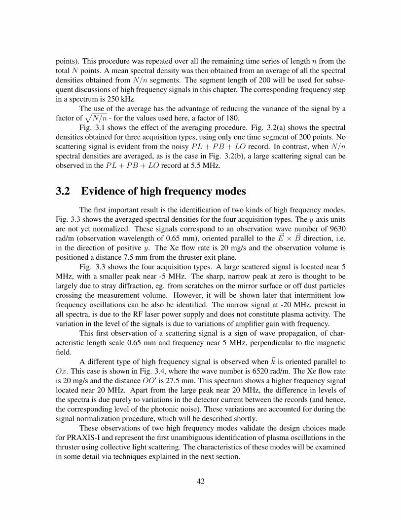
points). This procedure was repeated over all the remaining time series of length n from thetotal N points. A mean spectral density was then obtained from an average of all the spectraldensities obtained from N/n segments. The segment length of 200 will be used for subse-quent discussions of high frequency signals in this chapter. The corresponding frequency stepin a spectrum is 250 kHz.
The use of the average has the advantage of reducing the variance of the signal by afactor of
√N/n - for the values used here, a factor of 180.
Fig. 3.1 shows the effect of the averaging procedure. Fig. 3.2(a) shows the spectraldensities obtained for three acquisition types, using only one time segment of 200 points. Noscattering signal is evident from the noisy PL + PB + LO record. In contrast, when N/nspectral densities are averaged, as is the case in Fig. 3.2(b), a large scattering signal can beobserved in the PL+ PB + LO record at 5.5 MHz.
3.2 Evidence of high frequency modesThe first important result is the identification of two kinds of high frequency modes.
Fig. 3.3 shows the averaged spectral densities for the four acquisition types. The y-axis unitsare not yet normalized. These signals correspond to an observation wave number of 9630rad/m (observation wavelength of 0.65 mm), oriented parallel to the ~E × ~B direction, i.e.in the direction of positive y. The Xe flow rate is 20 mg/s and the observation volume ispositioned a distance 7.5 mm from the thruster exit plane.
Fig. 3.3 shows the four acquisition types. A large scattered signal is located near 5MHz, with a smaller peak near -5 MHz. The sharp, narrow peak at zero is thought to belargely due to stray diffraction, eg. from scratches on the mirror surface or off dust particlescrossing the measurement volume. However, it will be shown later that intermittent lowfrequency oscillations can be also be identified. The narrow signal at -20 MHz, present inall spectra, is due to the RF laser power supply and does not constitute plasma activity. Thevariation in the level of the signals is due to variations of amplifier gain with frequency.
This first observation of a scattering signal is a sign of wave propagation, of char-acteristic length scale 0.65 mm and frequency near 5 MHz, perpendicular to the magneticfield.
A different type of high frequency signal is observed when ~k is oriented parallel toOx. This case is shown in Fig. 3.4, where the wave number is 6520 rad/m. The Xe flow rateis 20 mg/s and the distance OO′ is 27.5 mm. This spectrum shows a higher frequency signallocated near 20 MHz. Apart from the large peak near 20 MHz, the difference in levels ofthe spectra is due purely to variations in the detector current between the records (and hence,the corresponding level of the photonic noise). These variations are accounted for during thesignal normalization procedure, which will be described shortly.
These observations of two high frequency modes validate the design choices madefor PRAXIS-I and represent the first unambiguous identification of plasma oscillations in thethruster using collective light scattering. The characteristics of these modes will be examinedin some detail via techniques explained in the next section.
42

-2 -1 0 1 2
x 107
0
1
2
3
4
5
x 10-6
Frequency (Hz)
Signal amplitude (arbitrary units)
PL + PB + LO
PL + LO
PB + LO
(a) Raw spectra without averaging
-3 -2 -1 0 1 2 3
x 107
0
1
2
3
x 10-11
Frequency (Hz)
Signal amplitude (arbitrary units)
PL + PB + LO
PL + LO
PB + LO
(b) Raw spectra to which averaging procedure has been applied
Figure 3.2: Spectral averaging for the extraction of the plasma-scattered signal from noisydata
43
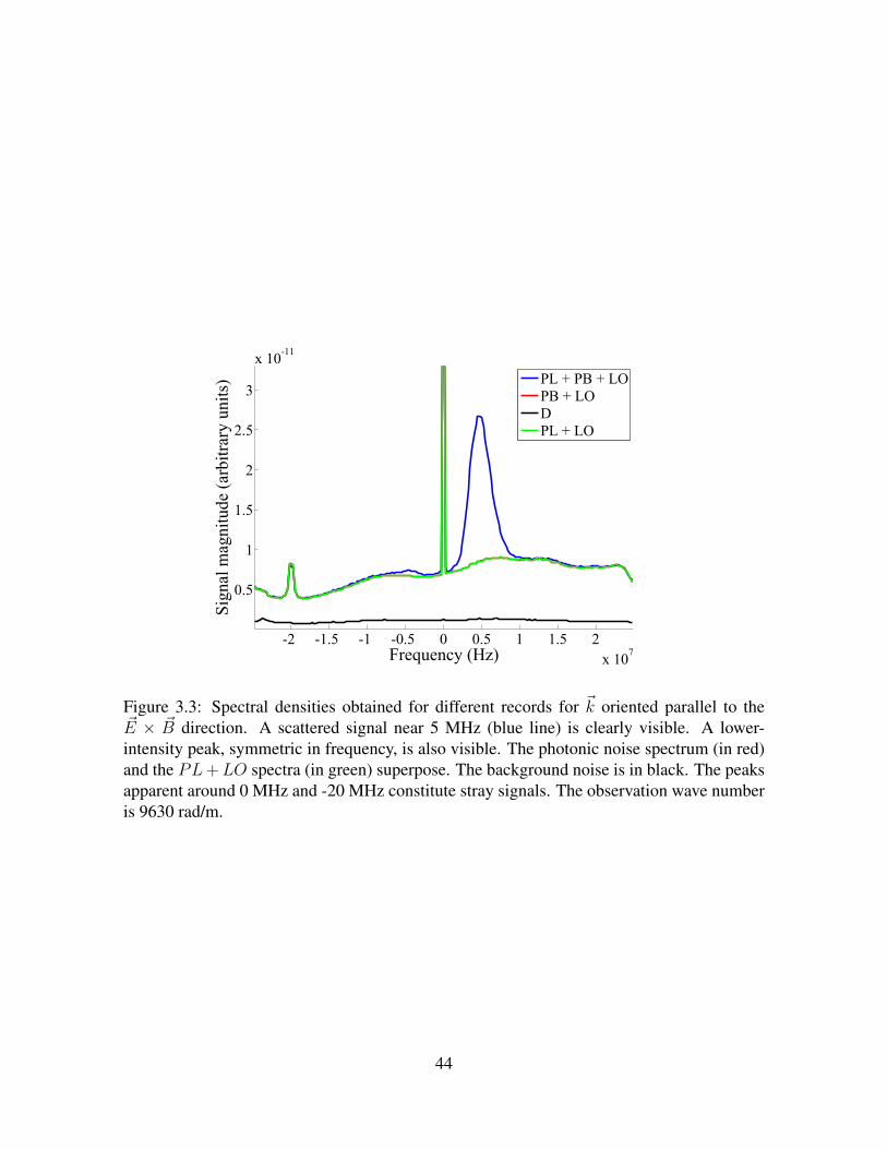
-2 -1.5 -1 -0.5 0 0.5 1 1.5 2
x 107
0.5
1
1.5
2
2.5
3
x 10-11
Frequency (Hz)
Signal m
agnitude (arb
itrary
units)
PL + PB + LO
PB + LO
D
PL + LO
Figure 3.3: Spectral densities obtained for different records for ~k oriented parallel to the~E × ~B direction. A scattered signal near 5 MHz (blue line) is clearly visible. A lower-intensity peak, symmetric in frequency, is also visible. The photonic noise spectrum (in red)and the PL+LO spectra (in green) superpose. The background noise is in black. The peaksapparent around 0 MHz and -20 MHz constitute stray signals. The observation wave numberis 9630 rad/m.
44

-2 -1 0 1 2
x 107
0
1
2
x 10-11
Frequency (Hz)
Signal magnitude (arbitrary units)
PL + PB + LO
PB + LO
D
PL + LO
Figure 3.4: Spectral densities obtained for different records for ~k oriented parallel to ~E. Thepresence of a broad, high frequency scattered signal around 20 MHz (blue line) is clear. Thepeaks apparent around 0 MHz and -20 MHz constitute stray signals. The observation wavenumber is 6520 rad/m.
3.3 Signal analysis techniquesA number of procedures were adopted to convert the raw signals into physical quan-
tities and determine absolute properties of the fluctuations.
3.3.1 Signal normalizationThe goal of the signal normalization is to isolate the collective scattering signal from
the noise, while removing artefacts such as variations in the amplifier gain over the frequencyrange and compensating for variations in the detector current between records.
The signal normalization procedure uses all four acquisition types in the followingway.
(a) The spectral density is calculated (arbitrary units) in the same manner for all four types:PL + PB + LO, PB + LO, PL + LO and D. First, the mean level of the cos and sinchannels over the full record is adjusted to zero (to eliminate any offsets which might bepresent), i.e.
Xn = Xn−Xn
where Xn represents the raw voltage reading versus time from either channel.
45

The level on both channels is divided by a mean value of the detector current, becausethe signal magnitude is proportional to the magnitude of this current. For the record withthe detector closed, the current value is arbitrarily set to 1 mA. Finally, the levels of thesin (“XB”) and cos (“XA”) channels relative to one another are adjusted,
XB = XB × σXA
σXB
where σXn is the standard deviation of the signal level.
The levels of the two channels are expected to be very similar. This adjustment of thesignal levels with respect to each other is intended to correct, if they exist, any minordifferences in the signal levels caused by differences in the mixers, amplifiers and filtersfor each channel. After these procedures, the spectral density is calculated as the meanspectral density of N/n segments (6.5×10⁶ / 200).
(b) The signal spectral density due only to the plasma scattering, Ψ(~k, ω)plasma is determinedas
Ψ(~k, ω)plasma = (Ψ(~k, ω)b × I2b )− (Ψ(~k, ω)c × Ic2)
where Ψ(~k, ω) represents the spectral density and I the mean value of the detector currentover the full record. The subscripts b and c denote PL+PB+LO and PB+LO recordsrespectively.
Similarly, the photonic noise signal Ψ(~k, ω)photonic is determined as
Ψ(~k, ω)photonic = (Ψ(~k, ω)a × Ia2)− (Ψ(~k, ω)d × Id2)
where the subscripts a and d represent PL+ LO and D records respectively.
The normalized signal spectral density Ψ(~k, ω)norm is then obtained from
Ψ(~k, ω)norm =Ψ(~k, ω)plasma
Ψ(~k, ω)photonic
(c) The normalized signal may now be converted to a physical quantity, the dynamic formfactor S(~k, ω), using the plasma and laser beam characteristics
S(~k, ω) =
(hν
ηPp
πw2
λ2r02
1
n0ls
)Ψ(~k, ω)norm (3.4)
where h, ν and r0 represent Planck’s constant, the incident wave frequency (2.83×10¹³
Hz), and the Thomson radius (2.8×10⁻¹⁵ m), respectively. η, the detector efficiency, is0.7. The primary beam power, Pp, is 42 W. The beam waist in the measurement zone, w,
46

is 2.5 mm, and the scattering length ls is 50 mm (twice the thruster channel width). Theelectron density n0 is not precisely known in the measurement zone, but it is on the orderof 1017 - 1018 m−3. The value of 1018 m−3 will be used.
S(~k, ω) has units of seconds. The dynamic form factor is a measure of the intensity ofthe density fluctuations over a range of frequencies. Fig. 3.5 shows the calculated dynamicform factor corresponding to the signal considered in Fig. 3.3. Signal artefacts have beenremoved and the symmetric scattering signal peaks are clearly distinguishable from the noise.
-3 -2 -1 0 1 2 3
x 107
-4
-2
0
2
4
6
8x 10
-4
Frequency (Hz)
Dynamic form factor (s)
Figure 3.5: The dynamic form factor of the ~E× ~B mode, corresponding to the data shown inFig. 3.3, obtained after signal normalization
3.3.2 Static form factorOnce the signal due to plasma scattering has been identified, a more useful form for
quantifying the mean square amplitude of the mode, at a particular wave number, is the staticform factor S(~k). This is the dynamic form factor integrated over an appropriate frequencyrange,
S(~k) =
∫S(~k, ω)
dω
2π(3.5)
The value of this integral is approximated by limiting it to the frequency limits forwhich the scattering signal is present. These frequency limits are easy to identify with a largeenough signal, after the normalization procedure. For the positive frequency peak in Fig. 3.5,the integration limits are 1 and 10 MHz. The static form factor for the modes identified is
47
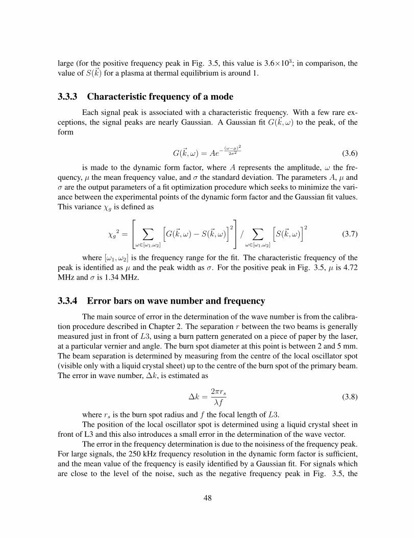
large (for the positive frequency peak in Fig. 3.5, this value is 3.6×10³; in comparison, thevalue of S(~k) for a plasma at thermal equilibrium is around 1.
3.3.3 Characteristic frequency of a modeEach signal peak is associated with a characteristic frequency. With a few rare ex-
ceptions, the signal peaks are nearly Gaussian. A Gaussian fit G(~k, ω) to the peak, of theform
G(~k, ω) = Ae−(ω−µ)2
2σ2 (3.6)
is made to the dynamic form factor, where A represents the amplitude, ω the fre-quency, µ the mean frequency value, and σ the standard deviation. The parameters A, µ andσ are the output parameters of a fit optimization procedure which seeks to minimize the vari-ance between the experimental points of the dynamic form factor and the Gaussian fit values.This variance χg is defined as
χg2 =
∑ω∈[ω1,ω2]
[G(~k, ω)− S(~k, ω)
]2
/ ∑ω∈[ω1,ω2]
[S(~k, ω)
]2
(3.7)
where [ω1, ω2] is the frequency range for the fit. The characteristic frequency of thepeak is identified as µ and the peak width as σ. For the positive peak in Fig. 3.5, µ is 4.72MHz and σ is 1.34 MHz.
3.3.4 Error bars on wave number and frequencyThe main source of error in the determination of the wave number is from the calibra-
tion procedure described in Chapter 2. The separation r between the two beams is generallymeasured just in front of L3, using a burn pattern generated on a piece of paper by the laser,at a particular vernier and angle. The burn spot diameter at this point is between 2 and 5 mm.The beam separation is determined by measuring from the centre of the local oscillator spot(visible only with a liquid crystal sheet) up to the centre of the burn spot of the primary beam.The error in wave number, ∆k, is estimated as
∆k =2πrsλf
(3.8)
where rs is the burn spot radius and f the focal length of L3.The position of the local oscillator spot is determined using a liquid crystal sheet in
front of L3 and this also introduces a small error in the determination of the wave vector.The error in the frequency determination is due to the noisiness of the frequency peak.
For large signals, the 250 kHz frequency resolution in the dynamic form factor is sufficient,and the mean value of the frequency is easily identified by a Gaussian fit. For signals whichare close to the level of the noise, such as the negative frequency peak in Fig. 3.5, the
48
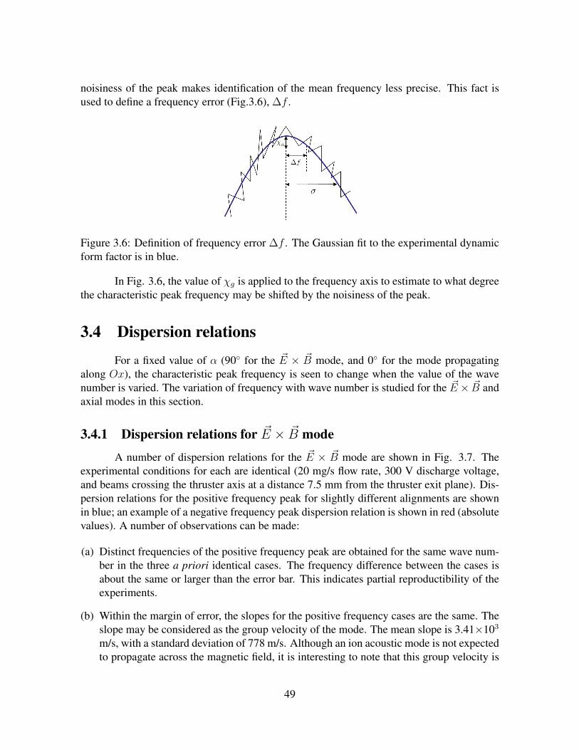
noisiness of the peak makes identification of the mean frequency less precise. This fact isused to define a frequency error (Fig.3.6), ∆f .
Figure 3.6: Definition of frequency error ∆f . The Gaussian fit to the experimental dynamicform factor is in blue.
In Fig. 3.6, the value of χg is applied to the frequency axis to estimate to what degreethe characteristic peak frequency may be shifted by the noisiness of the peak.
3.4 Dispersion relations
For a fixed value of α (90 for the ~E × ~B mode, and 0 for the mode propagatingalong Ox), the characteristic peak frequency is seen to change when the value of the wavenumber is varied. The variation of frequency with wave number is studied for the ~E × ~B andaxial modes in this section.
3.4.1 Dispersion relations for ~E × ~B mode
A number of dispersion relations for the ~E × ~B mode are shown in Fig. 3.7. Theexperimental conditions for each are identical (20 mg/s flow rate, 300 V discharge voltage,and beams crossing the thruster axis at a distance 7.5 mm from the thruster exit plane). Dis-persion relations for the positive frequency peak for slightly different alignments are shownin blue; an example of a negative frequency peak dispersion relation is shown in red (absolutevalues). A number of observations can be made:
(a) Distinct frequencies of the positive frequency peak are obtained for the same wave num-ber in the three a priori identical cases. The frequency difference between the cases isabout the same or larger than the error bar. This indicates partial reproductibility of theexperiments.
(b) Within the margin of error, the slopes for the positive frequency cases are the same. Theslope may be considered as the group velocity of the mode. The mean slope is 3.41×10³
m/s, with a standard deviation of 778 m/s. Although an ion acoustic mode is not expectedto propagate across the magnetic field, it is interesting to note that this group velocity is
49

0 2000 4000 6000 8000 10000 12000 140000
2
4
6
8
10x 10
6
Frequency (Hz)
k (rad.m-1)
Figure 3.7: Dispersion relations for the ~E × ~B mode. Dispersion relations for the positivefrequency peak, for identical experimental conditions but different alignments, are in blue.The dispersion relation for a negative frequency peak is shown in red (absolute values).
on the same order of magnitude as that of an ion acoustic mode propagating in a plasmawith an electron temperature of a few tens of eV.
(c) The near-identical linear slopes of the positive and negative frequency peaks suggest thatthese symmetric frequency peaks concern the same mode. The large difference in thepeak amplitudes, evident in Fig. 3.5, must therefore be accounted for.
(d) Most experiments were conducted at a high Xe flow rate (20 mg/s) because this was seento provide a large signal amplitude. The effect of different flow rates on the dispersionrelation is shown in Fig. 3.8, where flow rates are 6 and 20 mg/s. The larger flow ratecorresponds to the larger group velocity.
3.4.2 Dispersion relations for the axial modeThe axial mode has frequencies an order of magnitude larger than the those of the
~E × ~B mode. A dispersion relation for ~k oriented parallel to the jet axis is shown in Fig. 3.9.The Xe flow rate is 20 mg/s and the discharge voltage 300 V.
The upper range in k for this experiment was limited by practical reasons. The fre-quency of the peak increases with wavenumber, beyond the range of the filters, and the fre-quencies can no longer be (accurately) identified, even though the signal is still large. Theaxial mode presents some interesting features.
50

0 2000 4000 6000 8000 10000 120000
1
2
3
4
5
6x 10
6
Frequency (Hz)
k (rad.m-1)
Figure 3.8: Dispersion relations for the ~E× ~B mode at different flow rates (in blue - 20 mg/s,in red - 6 mg/s)
0 1000 2000 3000 4000 5000 60000
0.5
1
1.5
2
x 107
Frequency (Hz)
k (rad.m-1)
Figure 3.9: Dispersion relation for the axially-propagating mode
51

(a) The dispersion relation, as for the ~E × ~B mode, is linear. The group velocity associatedwith the slope is 15.5×10³ m/s. This value is, interestingly, close to the ion beam velocitymeasured using laser-induced fluorescence [26] (a little less than 20×103 m/s for similarparameters of the motor used). This axial mode appears to correspond to the sweepingof electrons by ions ejected at the thruster exit.
(b) The sign of the observed peak frequency is positive. This is because the wave vector isoriented in the same direction as the phase velocity of a mode moving in the direction ofpositive Ox (Fig. 3.1).
(c) The intercept of the line is 0.6×10⁷ Hz. Clearly, the relationship between the measuredgroup velocity and the frequency is more complicated than a simple Doppler relation.The value of the frequency intercept is on the order of the ion plasma frequency, whichwill be discussed later.
3.5 Peak width of the ~E × ~B modeA closer examination of the form of the frequency peak reveals interesting features.
The signals are not fine spectral lines, but broad peaks. The natural peak width due to thefinite resolution of the diagnostic is obtained from
∆f =δktvg2π
(3.9)
where δkt is the device wave number resolution (Eq. 1.15). The resulting value of∆f is 307 kHz, much smaller than the peak width determined for Fig. 3.5.
The peak half-widths for an experiment as a function of the wave number (the ~E× ~Bmode, 20 mg/s flow rate, 300 V discharge voltage) are shown in Fig. 3.10.
The peak width increases linearly with wave number, with a slope of 753.5 m/s and ay-intercept of 293 kHz (nearly identical to the computed device resolution ∆f , which is whatwould be expected). Were the peak width due purely to the device resolution, there would beno reason for it to increase with wave number, as is the case in Fig. 3.10.
Clearly, some physical mechanism influences the peak width. Two likely explana-tions may be proposed. First, electron temperature non-uniformities in the ion acoustic ve-locity and azimuthal drift velocity VD would tend to broaden the range of phase velocitiescontributing to the shape of the peak. The linear increase with wave number would be due tothe fact that the frequency width is the product of the spatial dispersion in phase velocity andthe wave number.
Secondly, damping effects could broaden the definition of the mean peak frequency.If the mode observed is due to resonance excitation by a background, broadband frequencysource, then the expected peak profile Pk(ω), at a particular wave number, as a resonantfunction of frequency ω may be written as a Lorentzian of the form
Pk(ω) = P0
[γk
2
(ω − ωk)2 + γk2
](3.10)
52

0 2000 4000 6000 8000 10000 120000
0.5
1
1.5
2x 10
6
Frequency (Hz)
k (rad.m-1)
Figure 3.10: Peak half-widths for the ~E × ~B mode as a function of wave number
where the frequency width at a particular wave number, represented by γk, is also theresonance damping rate. The peak mean frequency is ωk. The actual profile is a convolutionof the Lorentzian profile resulting from the resonance and the inherent Gaussian profile of thediagnostic. This convolution produces a Voigt profile, with a Gaussian central portion andLorentzian wings. The convoluted spectral width, ∆ωv may be estimated from the Gaussianwidth σg and Lorentzian width γk,
∆ωv =√γk2 + σg2 (3.11)
Since the observed spectral width ∆ωv is much larger than the Gaussian resolutionwidth, ∆ωv ≈ γk. The damping ratio for the convoluted fit can be approximated as γk/ωk,which is a constant value. From Fig. 3.10, the calculated damping ratio γk/ωk is 0.21.
Fig. 3.11 shows a comparison of the Lorentzian and Gaussian fits to the normalizedspectrum for the ~E × ~B mode at large wave number (k = 12600 rad/m), at which dampingeffects should be more apparent.
The Gaussian fit provides a better fit to the right hand and central portions of thespectrum, but the Lorentzian fits much better to the right hand side of the spectrum. A moreaccurate investigation of damping can only be done with a Voigt fit to the entire profile. Thisis, however, impossible given the low amplitude of the spectra at large wave numbers; anylong tails in the spectra become difficult to distinguish from the noise.
53
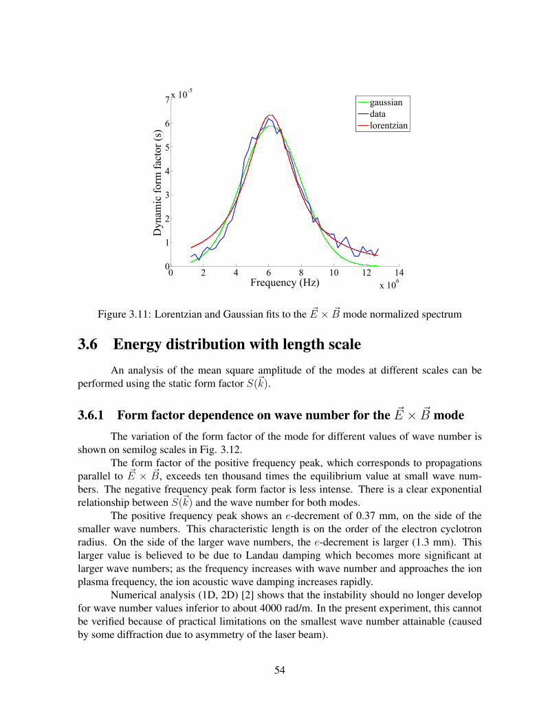
0 2 4 6 8 10 12 14
x 106
0
1
2
3
4
5
6
7x 10
-5
Frequency (Hz)
Dynam
ic form
fac
tor (s)
gaussian
data
lorentzian
Figure 3.11: Lorentzian and Gaussian fits to the ~E × ~B mode normalized spectrum
3.6 Energy distribution with length scaleAn analysis of the mean square amplitude of the modes at different scales can be
performed using the static form factor S(~k).
3.6.1 Form factor dependence on wave number for the ~E × ~B modeThe variation of the form factor of the mode for different values of wave number is
shown on semilog scales in Fig. 3.12.The form factor of the positive frequency peak, which corresponds to propagations
parallel to ~E × ~B, exceeds ten thousand times the equilibrium value at small wave num-bers. The negative frequency peak form factor is less intense. There is a clear exponentialrelationship between S(~k) and the wave number for both modes.
The positive frequency peak shows an e-decrement of 0.37 mm, on the side of thesmaller wave numbers. This characteristic length is on the order of the electron cyclotronradius. On the side of the larger wave numbers, the e-decrement is larger (1.3 mm). Thislarger value is believed to be due to Landau damping which becomes more significant atlarger wave numbers; as the frequency increases with wave number and approaches the ionplasma frequency, the ion acoustic wave damping increases rapidly.
Numerical analysis (1D, 2D) [2] shows that the instability should no longer developfor wave number values inferior to about 4000 rad/m. In the present experiment, this cannotbe verified because of practical limitations on the smallest wave number attainable (causedby some diffraction due to asymmetry of the laser beam).
54

0 2000 4000 6000 8000 10000 120001.5
2
2.5
3
3.5
4
4.5
log10[S(k)]
k (rad.m-1)
Figure 3.12: Exponential variation of form factor S(~k) with wave number for the ~E × ~Bmode. The positive frequency peak data is in blue, the negative frequency peak in red
The negative frequency peak has an e-decrement of 0.45 mm. The ratio of the positiveand negative peak intensities is around 30 and is maintained over the range of wave vectorvalues.
These observations permit additional interpretations about the origins of the negativefrequency peak. Certain hypotheses about its origin are proposed and each point is discussedseparately below.
(a) The negative frequency peak may be due to “ghosting” in the electronics. If the twomixed channels are not perfectly in quadrature, a small residual image of the positive fre-quency peak may be present at the negative frequency. In order to determine conclusivelyif this played a role in the presence of the negative peak, an experiment was conductedin still air to measure the level of an acoustic wave propagating in one direction (cor-responding to a positive frequency peak). The resulting signal spectra show a negativepeak due to ghosting, at a level 27 dB below the positive frequency peak. In comparison,for the plasma scattering experiment, the level of the negative frequency peak is over 15dB above this stray peak. Hence the negative frequency signal observed in this and otherexperiments is indeed due to plasma oscillations.
(b) The presence of the negative frequency peak may be due to oscillations propagating inthe opposite direction to the wave vector. Fig. 3.13 will be used here to describe theazimuthal positions on the thruster circumference. The plasma volume is in light blue,the measurement volume in grey.
55

Figure 3.13: Reference for azimuthal positions on thruster (referred to as clock hours). Thethruster plume is directed out of the page
At the 09h00 position, ~k is oriented upwards, in the same direction as the ~E × ~B drift.There are two likely possibilities: (i) a wave may be propagating in the same side ofthe thruster channel, but in the reverse direction, giving rise to the negative frequencypeak, or (ii) the negative frequency peak corresponds to the same wave as the positivefrequency peak, but measured in the opposite channel (03h00) where it would now bepropagating opposed to ~k.
(c) The difference in intensity of the two peaks could be due to the differing sensitivities inthe observation volume. The observation volume, a lozenge, has different sensitivitiesalong on its length, due to the Gaussian profiles of the intersecting beams. If the lozengeis not positioned on Oz such that its centre coincides with the thruster axis (Fig. 3.1), theamplitudes of the positive and negative peaks would be different (if these peaks corre-sponded to fluctuations in opposite sides of the channel). The longitudinal dimension ofthe observation volume, ll, has a minimum value of 21 cm (for a maximum experimentalangle of 21.25 mrad), and a maximum value of 48 cm (for a minimum experimental angleof 9.3 mrad). In comparison, the outer thruster diameter is 15 cm. The maximum errorin the positioning along Oz is between 0 and 20 cm. This corresponds to a sensitivityratio of between 1 and 0.16. The amplitude ratio of the negative frequency and positivefrequency peaks is 0.033, smaller than than five times the smallest sensitivity ratio.
If the negative frequency peak were attributed to fluctuations in the 03h00 side of thechannel, the amplitude of this peak would be five times (for O shifted off axis by 20 cm)to thirty times (forO shifted by 0 cm) smaller than the amplitude of the positive frequencypeak situated at 09h00. Even taking into account possible sensitivity differences dueto the positioning of the measurement volume, if the peaks do indeed correspond tofluctuations on either side of the channel, the fluctuations are not azimuthally symmetric.
56

3.7 Frequency dependence on position along the thrusteraxis 0′x
Thruster characteristics are known to evolve rapidly from inside the channel to theexterior, over a length of a few millimeters. These characteristics include the ion axial ve-locity profile, the electric field and the magnetic field. For this reason, it is interesting toexamine how the ~E × ~B and axial mode frequencies evolve with distance along O′x. Forboth cases, the observation wave number is fixed at a value of about 6200 rad/m, a relativelysmall value chosen to provide a large signal amplitude, and sufficiently small for the axialmode frequency to be identifiable within the limits imposed by the filters. There is no reasonto suppose that the frequency characteristics observed are wave number-specific.
An experiment to determine the evolution of the frequency and energy of both modesis performed by translating the thruster on its axis (the thruster is attached to a retractablearm which allows its axial position relative to the beams to be varied). The closest approachof the observation volume centre to the thruster exit is 7.5 mm. Some observations about themodes are made below.
3.7.1 Frequency dependence on axial position for the ~E × ~B modeThe variation of frequency with axial position is shown in Fig. 3.14.
0 10 20 30 40 50 60 70 800
0.5
1
1.5
2
2.5
3
3.5x 10
6
Frequency (Hz)
Distance from thruster exit plane (mm)
Figure 3.14: Frequency variation with axial distance from the thruster exit plane for the ~E× ~Bmode
The frequency steadily decreases from a value of 2.7 to 1.6 MHz over a distance ofabout 70 mm from the thruster exit plane. For our thruster operating parameters, the electric
57
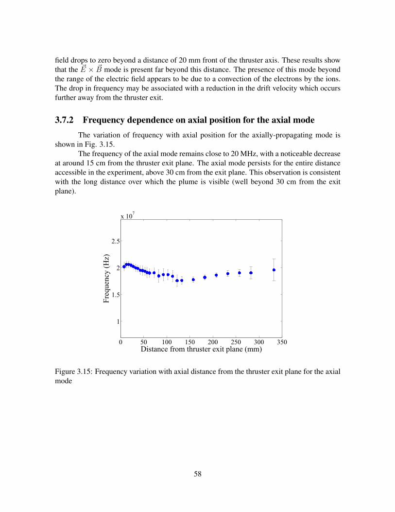
field drops to zero beyond a distance of 20 mm front of the thruster axis. These results showthat the ~E × ~B mode is present far beyond this distance. The presence of this mode beyondthe range of the electric field appears to be due to a convection of the electrons by the ions.The drop in frequency may be associated with a reduction in the drift velocity which occursfurther away from the thruster exit.
3.7.2 Frequency dependence on axial position for the axial modeThe variation of frequency with axial position for the axially-propagating mode is
shown in Fig. 3.15.The frequency of the axial mode remains close to 20 MHz, with a noticeable decrease
at around 15 cm from the thruster exit plane. The axial mode persists for the entire distanceaccessible in the experiment, above 30 cm from the exit plane. This observation is consistentwith the long distance over which the plume is visible (well beyond 30 cm from the exitplane).
0 50 100 150 200 250 300 350
1
1.5
2
2.5
x 107
Fre
quen
cy (
Hz)
Distance from thruster exit plane (mm)
Figure 3.15: Frequency variation with axial distance from the thruster exit plane for the axialmode
58

3.8 Form factor dependence on position along the thrusteraxis 0′x
3.8.1 Form factor dependence on axial position for the ~E × ~B mode
Fig. 3.16 shows the form factor measured at different distances for the ~E × ~B mode.
0 20 40 60 80 1001.5
2
2.5
3
3.5
4
4.5
log10[S(k)]
Distance from thruster exit plane (mm)
Figure 3.16: Form factor variation with axial distance from the thruster exit plane for the~E × ~B mode
The ~E × ~B mode, which has a short persistence in space, has an exponential energydecrease with distance. The corresponding e-decrement is 12.85 mm. The energy of themode is increases to a maximum at a distance of 13.5 mm from the thruster exit plane beforedecreasing. This is in fact consistent with numerical models (e.g. [42]) which show thefluctuation level and the anomalous electron mobility increasing beyond the thruster exitplane.
3.8.2 Form factor dependence on axial position for the axial modeThe form factor variation with distance from the exit plane for the axial mode is shown
in Fig. 3.17.The energy of the axial mode also reaches a maximum at 13.5 mm from the thruster
exit, and then decreases. The maximum fluctuation intensity of this mode is only 20% ofthe maximum fluctuation intensity for the ~E × ~B mode at a comparable wave number. Thispattern of much weaker fluctuations in the axial direction in the vicinity of the thruster exithas been repeatedly observed. The energy of the axial mode increases beyond 100 mm and
59
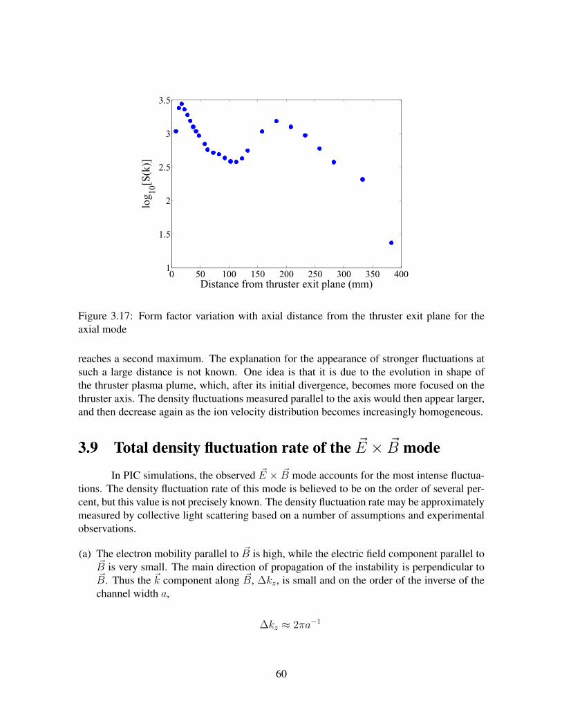
0 50 100 150 200 250 300 350 4001
1.5
2
2.5
3
3.5
log10[S(k)]
Distance from thruster exit plane (mm)
Figure 3.17: Form factor variation with axial distance from the thruster exit plane for theaxial mode
reaches a second maximum. The explanation for the appearance of stronger fluctuations atsuch a large distance is not known. One idea is that it is due to the evolution in shape ofthe thruster plasma plume, which, after its initial divergence, becomes more focused on thethruster axis. The density fluctuations measured parallel to the axis would then appear larger,and then decrease again as the ion velocity distribution becomes increasingly homogeneous.
3.9 Total density fluctuation rate of the ~E × ~B mode
In PIC simulations, the observed ~E × ~B mode accounts for the most intense fluctua-tions. The density fluctuation rate of this mode is believed to be on the order of several per-cent, but this value is not precisely known. The density fluctuation rate may be approximatelymeasured by collective light scattering based on a number of assumptions and experimentalobservations.
(a) The electron mobility parallel to ~B is high, while the electric field component parallel to~B is very small. The main direction of propagation of the instability is perpendicular to~B. Thus the ~k component along ~B, ∆kz, is small and on the order of the inverse of thechannel width a,
∆kz ≈ 2πa−1
60
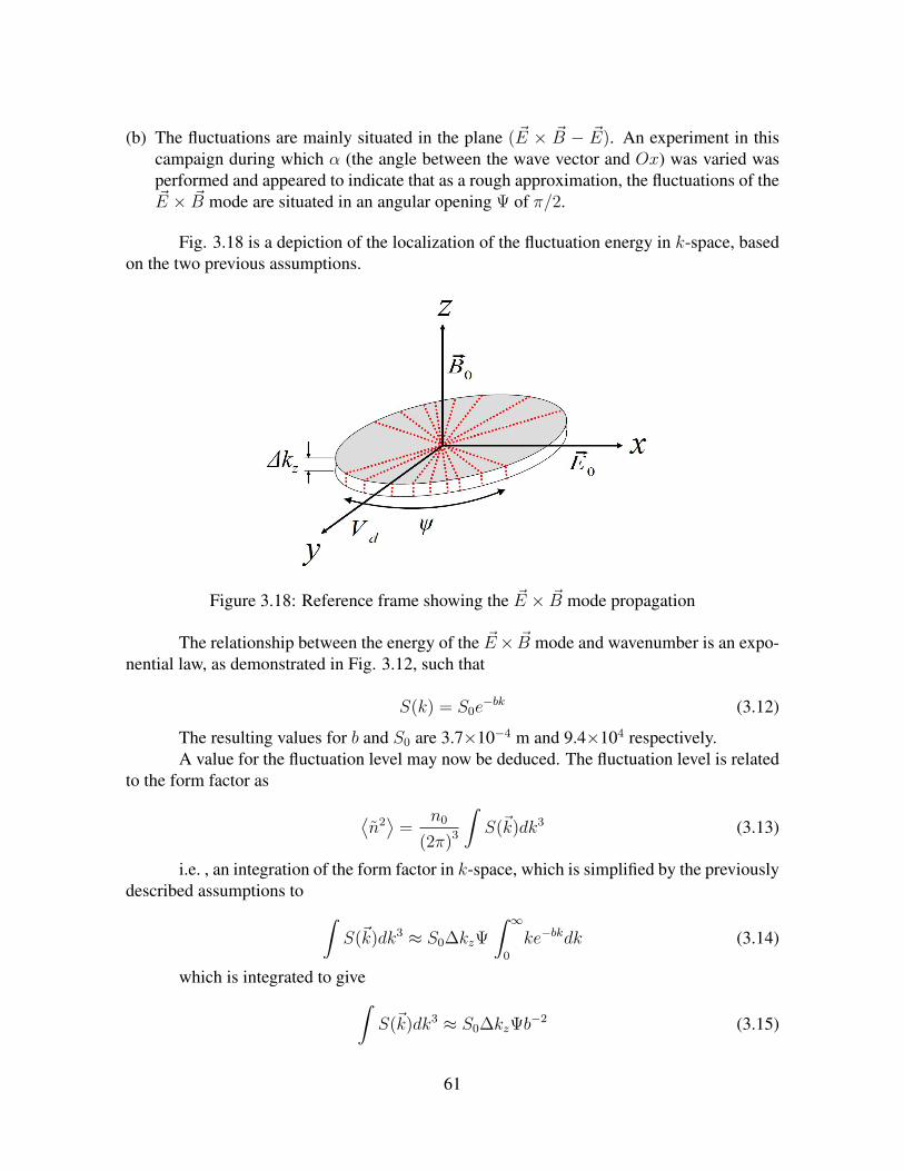
(b) The fluctuations are mainly situated in the plane ( ~E × ~B − ~E). An experiment in thiscampaign during which α (the angle between the wave vector and Ox) was varied wasperformed and appeared to indicate that as a rough approximation, the fluctuations of the~E × ~B mode are situated in an angular opening Ψ of π/2.
Fig. 3.18 is a depiction of the localization of the fluctuation energy in k-space, basedon the two previous assumptions.
Figure 3.18: Reference frame showing the ~E × ~B mode propagation
The relationship between the energy of the ~E× ~B mode and wavenumber is an expo-nential law, as demonstrated in Fig. 3.12, such that
S(k) = S0e−bk (3.12)
The resulting values for b and S0 are 3.7×10⁻⁴ m and 9.4×10⁴ respectively.A value for the fluctuation level may now be deduced. The fluctuation level is related
to the form factor as ⟨n2⟩
=n0
(2π)3
∫S(~k)dk3 (3.13)
i.e. , an integration of the form factor in k-space, which is simplified by the previouslydescribed assumptions to ∫
S(~k)dk3 ≈ S0∆kzΨ
∫0
∞ke−bkdk (3.14)
which is integrated to give∫S(~k)dk3 ≈ S0∆kzΨb
−2 (3.15)
61

The r.m.s density fluctuation level 〈n2〉1/2 thus obtained is 4×10¹⁴ m−3. The meanplasma density n0 in Eq. 3.13 is cancelled out by the corresponding mean density used inEq. 3.4, and therefore this r.m.s density fluctuation is an absolute value. The r.m.s densityfluctuation rate, obtained using a mean plasma density of 1018 m−3, is then
〈n2〉1/2
n0
≈ 4× 10⁻⁴ (3.16)
This value is very small, less than 0.1%. Before interpreting the significance of thislevel, it is worth bearing in mind a number of points:
(a) The determination of the fluctuation rate depends on a knowledge of the mean plasmadensity, which was in this case chosen to be 1018 m−3, but whose value could easily bean order of magnitude smaller, in which case the fluctuation rate would be 4×10⁻³. Thevalue used is a typical plasma density in the region of the thruster exit obtained fromhybrid models.
(b) It is necessary to measure the angular opening of the mode more accurately. This wouldallow the fluctuation rate to be integrated over a precise range and account for the wavenumber component parallel to ~B. A better determination of the wave number componentparallel to ~B is also necessary.
(c) The optical bench was carefully designed for the measurement of a low level of electrondensity fluctuations. However, a calibration of the bench will be required to determine ifthe measured fluctuation level is in some way underestimated due to signal losses, due,for instance, to a poor heterodyning efficiency.
3.10 Further interpretations and analysis
3.10.1 A hypothetical determination of the electron temperature
The dispersion relation of the ~E× ~B mode shown in Section 3.4.1 provides interestingclues as to the properties of this mode.
Firstly, the mean value of this intercept in Fig. 3.7 is 133.7 kHz, with a standarddeviation of 436 kHz. The intercept value is quite close to zero, and considering the linearnature of this mode’s dispersion relation, its topology resembles that of an ion acoustic mode,with a group velocity vg corresponding to the slope. As mentioned earlier, the ion acousticmode is not expected to propagate strictly perpendicular to ~B for wavelengths on the orderof, or larger than, the electron cyclotron radius. However, since the ~B field is not entirelyuniform and the wavelength is small, an attempt at comparing the observed mode with thecharacteristics of an ion acoustic wave appears legitimate. The dispersion relation for suchan ion acoustic mode is
vg =δω
δk=
√kBTemi
(3.17)
62

where kB is Boltzmann’s constant and mi the Xenon ion mass.Hence an electron temperature may be estimated from the experimental dispersion
relation. The resulting value is 16 eV. Later experiments designed to determine the directionof propagation of this mode more precisely are able to show that there is in fact a smallk-component parallel to ~B.
For now, this estimate of the electron temperature will be used to determine severalcharacteristic velocities and frequencies.
3.10.2 Characteristic velocities, frequencies and length scales for the ex-periment
For reference, the thruster and plasma parameters are summarized in Table 3.1.
Parameter Symbol ValueElectric field E0 104 V/mMagnetic field B0 15×10−3 TXe ion mass mi 2.175×10⁻²⁵ kgelectron mass me 9.11×10⁻³¹ kgLocal electron density ne 1018 /m3
Local electron temperature Te 16 eV
Table 3.1: Thruster and plasma parameters
The resulting velocities, frequencies and length scales are given in Table 3.2.Taking these values into account, a further commentary on the experimental results
can be made.
3.10.3 Interpretations of the frequencies of the ~E × ~B and axial modes
The frequencies of the dispersion relation of the ~E × ~B mode (Fig. 3.7) are smalleror on the same order as the ion plasma frequency. This indicates that the ion and electronmotions are not strictly identical. One possible consequence of this decoupling is a dampingof the mode.
Concerning the axial mode, the non-zero frequency intercept suggests that the axialelectron movement can be regarded as a superposition of two motions. There is a convectionof electrons caused by the coupled ion species leaving the channel, and in addition, a coupledoscillation of the two species, with a frequency on the order of the ion plasma frequency. ADoppler frequency shift, linearly increasing with wave number, would then account for theobserved group velocity.
63

Parameter Definition ValueAzimuthal drift velocity Vd = E0/B0 6.67×10⁵ m/sElectron thermal velocity vthe =
√kTe/me 1.68×10⁶ m/s
Ion cyclotron angular frequency ωci = eB/mi 1.09×10⁴ rad/sIon plasma angular frequency ωpi =
√nee2/(ε0mi) 1.15×10⁸ rad/s
Electron cyclotron angular frequency ωce = eB/me 2.64×10⁹ rad/sElectron plasma angular frequency ωpe =
√nee2/(ε0me) 5.63×10¹⁰ rad/s
Ion cyclotron frequency ωci/2π 1.74×10³ HzLower hybrid frequency fLH ≈
√fcefci 8.55×10⁵ Hz
Ion plasma frequency ωpi/2π 18×106 HzElectron cyclotron frequency ωce/2π 4.20×10⁸ HzElectron plasma frequency ωpe/2π 8.97×10⁹ HzCyclotron drift length lce = 2πVd/ωce 1.59×10⁻³ mElectron Larmor radius ρce = vthe/ωce 6.36×10⁻⁴ mElectron Debye length λD = vthe/ωpe 2.98×10⁻⁵ mCyclotron drift wave number kc = ωce/Vd 3.93×10³ rad/mLarmor wave number kL = ρce
−1 1.57×10³ rad/mDebye wave number kD = λD
−1 3.35×10⁴ rad/mDoppler frequency, motion parallel to ~B ∆kzvthe 6.72×10⁷ rad/sDoppler frequency, ~E × ~B drift kcVd = (2πlc)Vd = ωce 2.64×10⁹ rad/s
Table 3.2: Characteristic plasma frequency and length scales
64

3.10.4 Experimental results in the context of linear theoryThese experimental results may now be considered in the context of the theoretical
predictions of Adam et. al. [2]. The theoretical approach used to determine the conditionsfor which the azimuthal drift instability arises is discussed.
Basic assumptions in linear theory
The coordinate system adopted places x coincident with the thruster axis, z parallelto the magnetic field, and y coincident with, but opposite in sign to, the azimuthal drift.
• The electric field is constant (E0) and purely axial; the magnetic field is constant (B0)and purely radial.
• The drift velocity Vd is sufficiently large that the magnetic field drift velocity and thedensity gradient drift velocity can be neglected.
• The ions are cold, immobile, and unaffected by the magnetic field.
• The electrons may be described by a shifted Maxwellian distribution function withisotropic temperature, of the form
f0 = n0
(me
2πkBTe
)3/2
exp
[−(~v − ~Vd)
2
2vthe2
](3.18)
Theoretical dispersion relations
Fluid equations are used to derive the perturbed ion density as a function of φ, andthe ion mean velocity and temperature are neglected. The electron velocity distribution issubstituted into the Vlasov equation, linearized as a function of the wave potential Φ andintegrated to give the perturbed electron density. These densities are substituted into Poisson’sequation to yield the dispersion relation, in simplified 2D form (by ignoring perturbationsparallel to ~B),
k⊥2λD
2
(1− me
mi
ωpe2
ω2
)+
[1− I0(b)e−b +
n=∞∑n=1
2(ω − kyVd)2In(b)e−b
(nωce)2 − (ω − kyVd)2
]= 0 (3.19)
where k⊥2 = ky2 + kx
2. I0 and In are Bessel functions of order zero and n, whileb = (k⊥vthe/ωce)
2.This is further simplified (by neglecting perturbations parallel to the thruster axis, i.e.
kx = 0) to give the one dimensional dispersion relation,
ky2λD
2
(1− me
mi
ωpe2
ω2
)+
[1− I0(b)e−b +
n=∞∑n=1
2(ω − kyVd)2In(b)e−b
(nωce)2 − (ω − kyVd)2
]= 0 (3.20)
65

where b is now written as (kyvthe/ωce)2.
The perturbed electrostatic potential Φ is of the form
Φ = φ ei(~k·~r−(ωr+iγ)t) (3.21)
where k is real, and the complex frequency consists of the real ωr and the instabilitydamping frequency γ. The numerical solutions to these dispersion relations are now consid-ered in the context of our results.
Numerical solution of the one- and two-dimensional dispersion relations
According to Eqs. 3.19 and 3.20, the transitions from stability to instability occur forresonances of kyVd/ωpe with the cyclotron harmonics nωce/ωpe, i.e.
kyVd ≈ nωce (3.22)
where n represents integer values.From Eq. 3.22, the transitions to instability would occur for
ky = 3.956× 10³n rad/m (3.23)
The experimental wave number range is 5480 to 12600 rad/m. In the experimentalrange, the instability would be expected only in the vicinity of 8500 and 12500 rad/m (i.e. n= 2 and n = 3 respectively).
The solution to the two-dimensional dispersion relation is shown in Fig. 3.19. Theparameters used to generate this figure have been chosen to cover the range of experimentalwavenumbers and plasma parameters: the plasma density used in the code has been set to1018 m−3, the ratio vthe/Vd to 2.5, and the ratio ωce/ωpe to 0.047. The frequencies and growthrates will be presented in Hz to aid direct comparisons to experimental results.
Fig. 3.19 shows the discrete nature of the two-dimensional theoretical dispersionrelation; the instability is restricted to the neighbourhood of certain values of ky only, whereasthe experimentally-obtained dispersion relation is continuous.
The imaginary part of the frequency (the growth rate of the instability) is shown inFig. 3.20.
As is evident from Figs. 3.19 and 3.20, the dependencies of the frequency and growthrate on kx are negligible. The exact form of the unstable regions as a function of ky canbe examined for a fixed kx value. kx is set to zero and the lobes corresponding to the one-dimensional solution are obtained.
Fig. 3.21 shows the comb-like form of the frequency lobes for kx=0. The frequen-cies expected experimentally fall between 10 and 20 MHz. The maximum growth rates aresimilarly localized about certain values of wave number (Fig. 3.22).
The experimental results, while consistent with the frequencies and wave numberspredicted for the instability by linear theory, do not reproduce the discrete nature of the the-oretical dispersion relation. The inherent resolution of the diagnostic, for the Gaussian beamwaist of 2.5 mm in the measurement zone, is about 570 rad/m. During an experiment, the
66
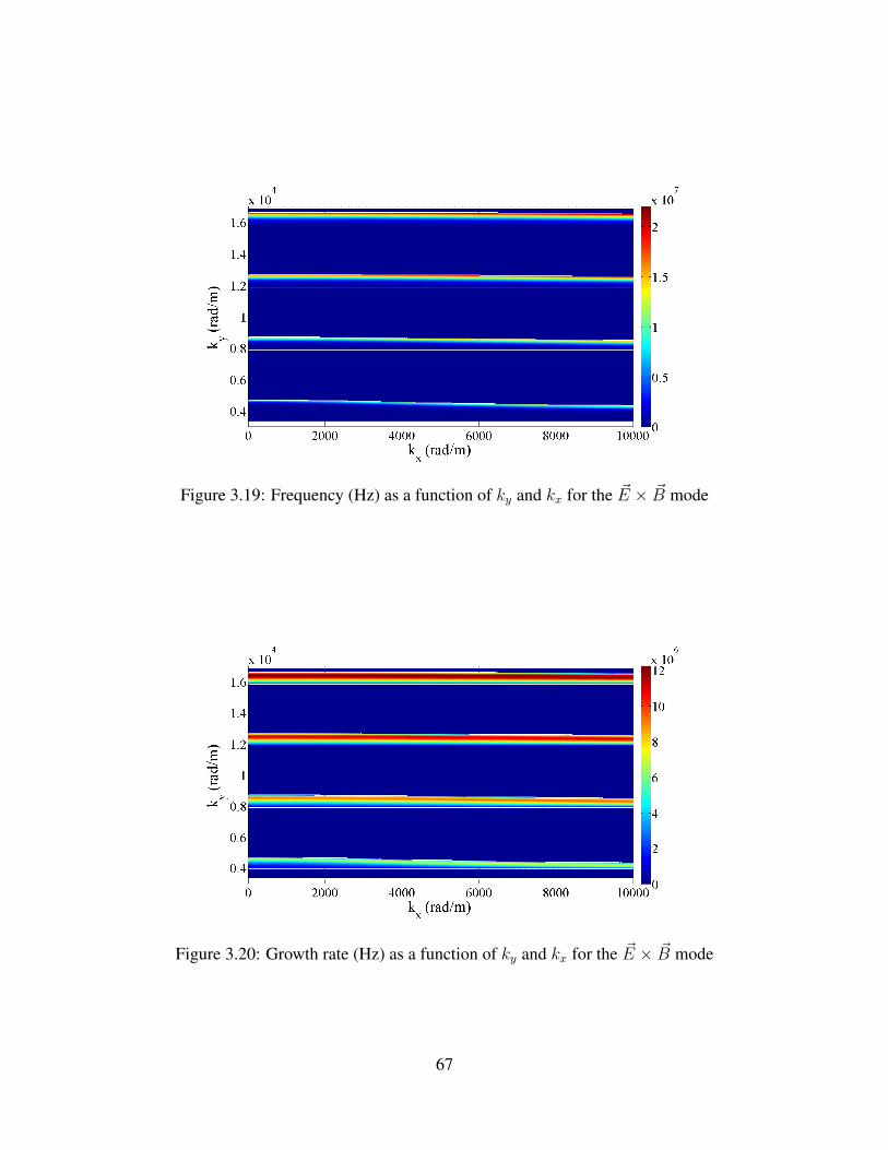
Figure 3.19: Frequency (Hz) as a function of ky and kx for the ~E × ~B mode
Figure 3.20: Growth rate (Hz) as a function of ky and kx for the ~E × ~B mode
67
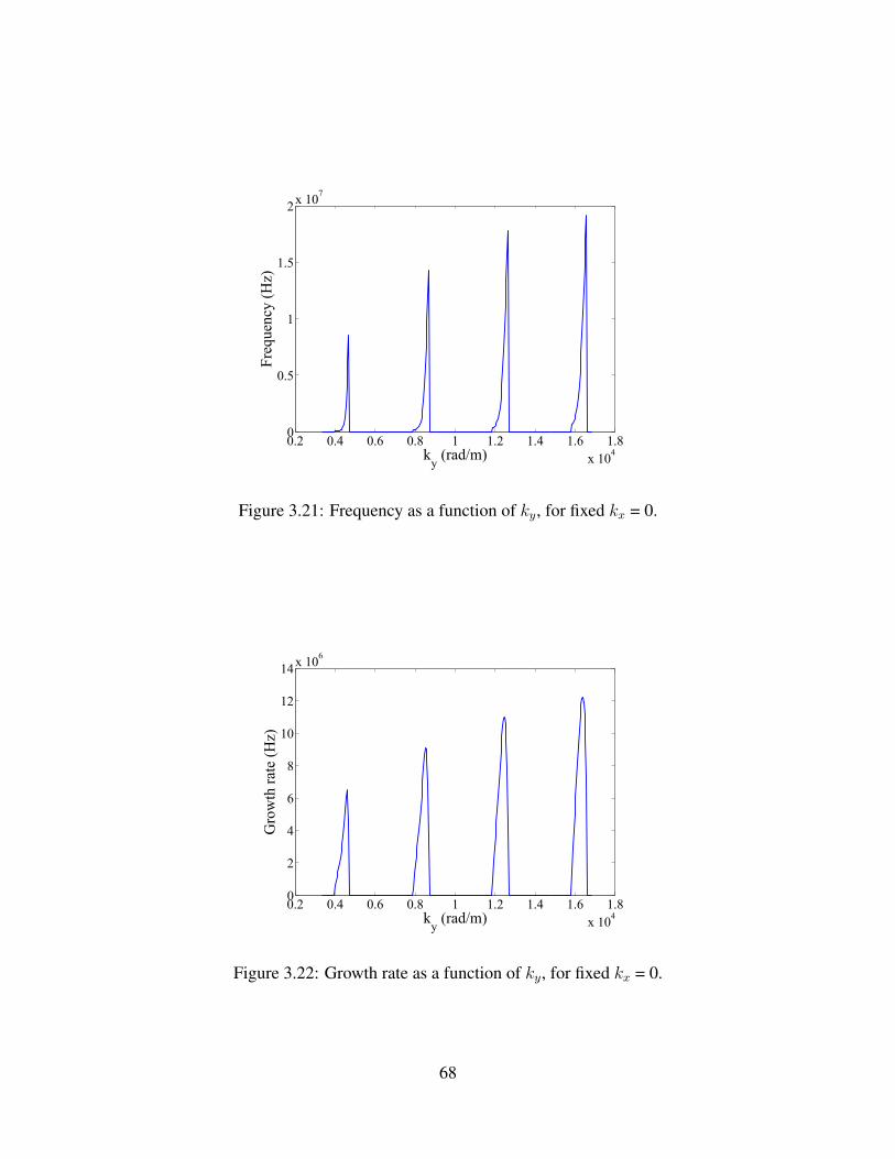
0.2 0.4 0.6 0.8 1 1.2 1.4 1.6 1.8
x 104
0
0.5
1
1.5
2x 10
7
ky (rad/m)
Frequency (Hz)
Figure 3.21: Frequency as a function of ky, for fixed kx = 0.
0.2 0.4 0.6 0.8 1 1.2 1.4 1.6 1.8
x 104
0
2
4
6
8
10
12
14x 10
6
ky (rad/m)
Growth rate (Hz)
Figure 3.22: Growth rate as a function of ky, for fixed kx = 0.
68

wave vector is typically varied in steps of 740 rad/m, which is on the same order as the de-vice resolution. Hence, neither the device resolution nor the experimental wave number stepjustify missing the unstable lobes, if they do exist.
For kx = 0, the dependence of frequency and growth rate on ky may be shown for avery large range of ky values (of which our range is only a small part). It has already beenobserved that the dispersion relation resembles a series of comb-like lobes (Figs. 3.21 and3.22). The maximum of each lobe (for wr and γ) is now associated with the ky value forwhich it appears. The resulting points are plotted over a range of ky from 0 to 17×105 rad/m.Each point therefore represents a particular lobe n. The values obtained for frequency andgrowth rate are shown in Figs. 3.23 and 3.24.
0 0.5 1 1.5 2
x 105
0.4
0.6
0.8
1
1.2
1.4
1.6
1.8
2x 10
7
ky (rad/m)
Frequency (Hz)
Figure 3.23: Characteristic lobe frequencies as a function of ky, for kx = 0.
Certain observations can be made concerning the instability.The first lobe accessible experimentally (n = 2) at ky = 8500 rad/m has a frequency
associated with the maximum growth rate at 6.6 MHz. The second lobe accessible experi-mentally (n = 3) at ky = 12500 rad/m has a frequency associated with the maximum growthrate at 8.4 MHz. Both frequency values are on the order of those seen during the experiment.The range used experimentally is very small compared to that shown in Fig. 3.23, but thelinearity seen in the experimental dispersion relation is not inconsistent with the numericalfindings at small ky. For larger ky values, the frequency reaches the ion plasma frequency, asexpected for an ion acoustic wave.
The growth rate characteristics are quite interesting. The lobes attainable experimen-tally are associated with growth rates of 9.1 MHz (n = 2) and 11.0 MHz (n = 3). Thesevalues are inferior to the maximum growth rate (13.4 MHz, seen at lobe n = 7, for which ky= 28100 rad/m), but still significant. Apparently, the maximum growth rate would only bevisible at small length scales of 0.2 mm. The experimentally-observed form factor of thesefluctuations is not compatible with this growth rate behaviour, since the form factor is large
69

0 0.5 1 1.5 2
x 105
4
6
8
10
12
14x 10
6
ky (rad/m)
Growth rate (Hz)
Figure 3.24: Characteristic growth rates as a function of ky, for kx = 0.
at larger scales and decays exponentially with wave number.It is possible the presence of gradients, in the drift velocity, for instance, which are
not accounted for in the model, may explain the non-discrete dispersion relation observedexperimentally. A radial gradient in Vd would reduce the growth rate, but the instabilitywould spread over the space in ky, rather than being restricted to narrow lobes. In addition,the electron thermal velocity vthe may not be constant. In fact, there are several electronpopulations of different energies present in the thruster [10] and this could also play a role inexpanding the range of the unstable lobes beyond certain limited ky values.
The main goal of these experiments has been achieved: the small-scale azimuthalinstability has been identified experimentally, in addition to an axial mode. The specially-designed collective scattering bench PRAXIS-I has proven capable of measuring the weakdensity fluctuations associated with this instability.
Apart from the qualitative similarity of the ~E× ~B mode characteristics and the predic-tions provided by linear theory, there are quantitative agreements. For similar wave numbers,the frequencies predicted by linear theory and those obtained experimentally are compara-ble. It has been observed that the component kx appears to affect only slightly the instabilityfrequency and growth rate, and this will be verified more carefully experimentally.
Linear dispersion relations and the form factor levels with length scale and positionalong the thruster axis have been obtained for both modes. The differences between the ex-perimental and theoretical dispersion relations may be accounted for by additional effects,such as gradients in drift velocity, a broad distribution of electron temperatures, and the pos-sible presence of a wave vector component parallel to the magnetic field. This will be studied
70
in more depth in Phase II.Concerning the theoretical results discussed in this chapter, an important assumption
was made during the development of the dispersion relation: that the electron distribution isMaxwellian. This greatly simplifies the solution of the equation, but restricts the validity ofthe solutions to a limited case. A. Ducrocq [17] studied the effect on the instability whendistorted distribution functions were applied. It was observed that the distortion reduced thewidth of the unstable lobes, and the value of ky for which the maximum growth rate was seenbecame smaller. The electron distribution represents a major unknown in the characterizationof the modes observed.
Despite the challenges involved in modelling the instability, thanks to these early ex-periments, a clearer picture of the azimuthal fluctuations is emerging. The second phase ofexperiments will attempt to resolve a number of new issues arising from the first campaign,such as obtaining a better characterization of the modes, determining their location and di-rectionality, and narrowing the gap between theory and experiment.
71

72

Part II
73

74

Chapter 4
PRAXIS-II
Contents4.1 Goals of Phase II experiments . . . . . . . . . . . . . . . . . . . . . . . 75
4.2 Changes to PRAXIS-I . . . . . . . . . . . . . . . . . . . . . . . . . . . . 76
4.3 PRAXIS-II design . . . . . . . . . . . . . . . . . . . . . . . . . . . . . . 77
4.3.1 Bench configuration . . . . . . . . . . . . . . . . . . . . . . . . . 77
4.3.2 Measurement of heterodyne efficiency . . . . . . . . . . . . . . . . 80
4.3.3 Verification of signal level . . . . . . . . . . . . . . . . . . . . . . 83
4.1 Goals of Phase II experiments
THE main goals of the second phase of experiments may be summarized as follows:
Reduce the minimum wave number : In order to view experimentally a possible saturationin the energy of the ~E × ~B mode at large scales, it is necessary to reduce the minimumwave number attainable, from 5480 to about 3900 rad/m, as shown in Eq. 3.23. Thisrequires a redesign of the optical bench and an improvement of the laser profile toreduce diffraction.
Determine the significance of the negative frequency ~E × ~B mode : The question was posedduring Phase I experiments as to whether the presence of the negative frequency peakwas due to an observation of the far side thruster channel (03h00), or whether thefluctuations occur in the same side as the positive frequency peak (at the 09h00 side).Experiments will be designed to clarify the origin of the negative frequency peak.
Determine the directionality of modes : A determination of how the modes propagate inspace requires experiments which can measure three wave vector components: in the
75

direction of the azimuthal drift, along the ion plume, and parallel to ~B. A knowledgeof the directionality of the modes would also allow a more accurate estimation of thedensity fluctuation rate.
Determine the true signal level : To determine if the signal level measured is the absolutesignal level, the diagnostic requires calibration, and a determination of possible hetero-dyning losses.
Explore the possible sources of experiment-theory discrepancies : Experiments to deter-mine the true signal level will verify whether the density fluctuations of this instabilityare indeed very small, contrary to numerical expectations. They will also determinewhether the two-dimensional view of the propagation of the instability is accurate.
Determine the relative level of density fluctuations along ~B : The density fluctuations alongthe magnetic field are expected to be very small, and their Doppler frequency very high,6.72×107 rad/s according to Table 3.2. Experiments designed to measure propagationsin this direction will be performed.
Determine effect of varying thruster parameters The influence of thruster parameters suchas flow rate, discharge voltage, and magnetic field on the azimuthal instability will bestudied.
To attain these goals, several new experiments are required, some of which are beyondthe capabilities of PRAXIS-I.
4.2 Changes to PRAXIS-IFor the second phase of experiments an upgraded optical bench with expanded capa-
bilities, PRAXIS-II, is built. Some of the main approaches used to adapt the optical benchare outlined below:
(a) Improvement of the laser profile: on PRAXIS-I, the laser beam was observed to be non-Gaussian, with an asymmetric profile and long tails. To avoid diffraction at the translator-rotator, which would result in a fraction of the primary beam reaching the detector, it wasnecessary to increase the minimum separation between the primary and local oscillatorbeams. This in turn increased the minimum wave number; the final minimum value onPRAXIS-I was 5480 rad/m. On PRAXIS-II, in order to achieve smaller wavenumbers,the laser beam is made to pass through a ceramic tube before division into its primary andlocal oscillator components. This tube, when precisely aligned, absorbs to some extentthe low-energy tails of the beam and renders the beam more symmetric.
(b) Expansion of the beam waist: the beam waist in the measurement zone is increased from2.5 mm to 2.9 mm, by the replacement of the lens L2 (focal length 1000 mm) withlenses of focal lengths 625 mm. This reduces the divergence of the beam as well as the
76

minimum attainable wave number: the k-resolution is now reduced to 975 rad/m, givinga minimum (theoretical) wave number attainable of about 3900 rad/m.
(c) Modifications to the translator-rotator: the range of rotation of the wave vector in theplane xOy was limited to 295 on PRAXIS-I because of the optical supports used formirror M8. The actual experimental range used in Phase I was only 90. In this secondphase of experiments, the optical supports are modified to allow the full 360 range ofrotation, of which 320 will be fully explored in the experiments. An angular openingof only 40 is unaccessible due to the modified optical support. This modification isintended to allow a much fuller map of the directionality of the modes.
4.3 PRAXIS-II design
4.3.1 Bench configurationThe modified design of PRAXIS-II is presented in Fig. 4.1. The naming conventions
observed in Fig. 2.1 are the same. CR represents the ceramic tube, which is positioned suchthat the minimum waist created by L1 is near the entry of the tube (21 mm in front of it).An additional lens L2 is used to fabricate a sufficiently small waist for entry into the AODwindow. The tube internal diameter is 4.80 mm, slightly under four times the beam waist(1.25 mm) at this location, and was determined adequate for the absorption of the long tailsof the beam. The tube length, 305 mm, is on the same order as the Rayleigh length. The powerloss due to the tube, from the initial laser power of 42 W, is about 19%. The recalculated M2
value post-tube is close to 1, whereas it was determined to be 1.2 on PRAXIS-I.The spacing of the important elements is given in Table 4.1, while the lens focal
lengths are summarized in Table 4.2. The beam waists and associated Rayleigh lengths aresummarized in Table 4.3.
Elements Separation (mm)Lw - L1 589L1 - entry CR 525entry CR - L2 375L2 - BS 75L2 - AOD 359AOD - L3 625L3 - M8 750L3 - L5 2750L4 - TR 750TR - L5 2000
Table 4.1: Summary of key distances on PRAXIS-II
77
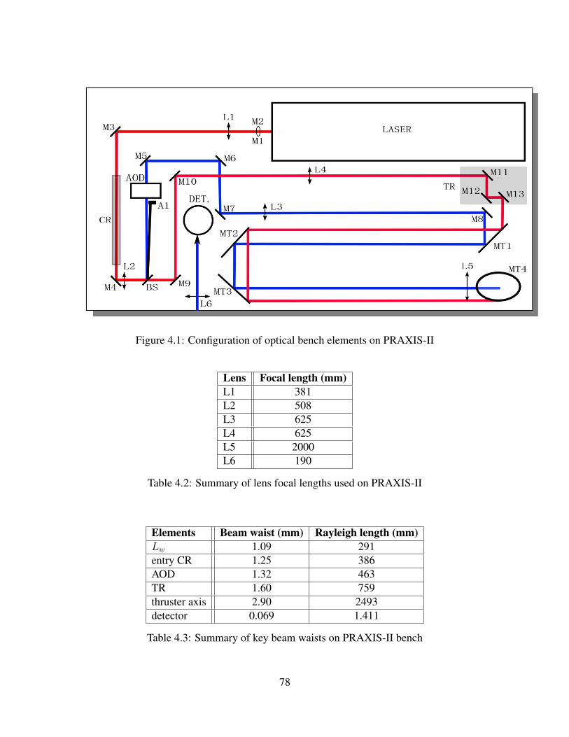
Figure 4.1: Configuration of optical bench elements on PRAXIS-II
Lens Focal length (mm)L1 381L2 508L3 625L4 625L5 2000L6 190
Table 4.2: Summary of lens focal lengths used on PRAXIS-II
Elements Beam waist (mm) Rayleigh length (mm)Lw 1.09 291entry CR 1.25 386AOD 1.32 463TR 1.60 759thruster axis 2.90 2493detector 0.069 1.411
Table 4.3: Summary of key beam waists on PRAXIS-II bench
78
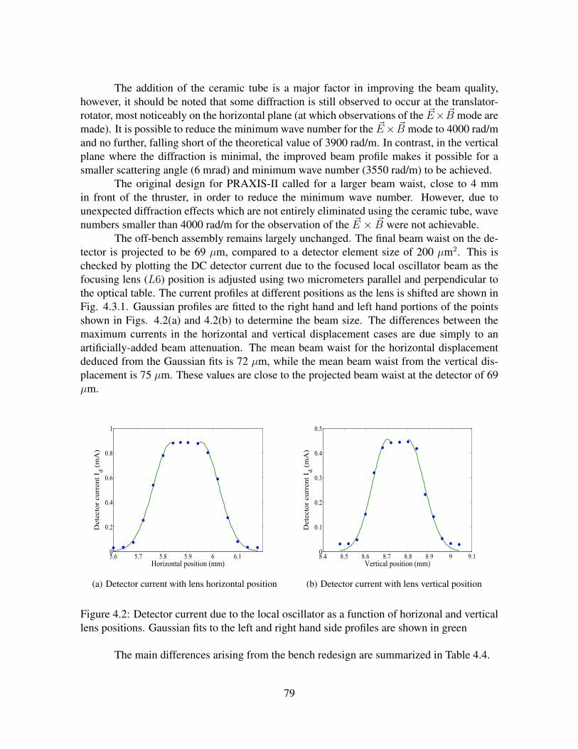
The addition of the ceramic tube is a major factor in improving the beam quality,however, it should be noted that some diffraction is still observed to occur at the translator-rotator, most noticeably on the horizontal plane (at which observations of the ~E× ~B mode aremade). It is possible to reduce the minimum wave number for the ~E× ~B mode to 4000 rad/mand no further, falling short of the theoretical value of 3900 rad/m. In contrast, in the verticalplane where the diffraction is minimal, the improved beam profile makes it possible for asmaller scattering angle (6 mrad) and minimum wave number (3550 rad/m) to be achieved.
The original design for PRAXIS-II called for a larger beam waist, close to 4 mmin front of the thruster, in order to reduce the minimum wave number. However, due tounexpected diffraction effects which are not entirely eliminated using the ceramic tube, wavenumbers smaller than 4000 rad/m for the observation of the ~E × ~B were not achievable.
The off-bench assembly remains largely unchanged. The final beam waist on the de-tector is projected to be 69 µm, compared to a detector element size of 200 µm2. This ischecked by plotting the DC detector current due to the focused local oscillator beam as thefocusing lens (L6) position is adjusted using two micrometers parallel and perpendicular tothe optical table. The current profiles at different positions as the lens is shifted are shown inFig. 4.3.1. Gaussian profiles are fitted to the right hand and left hand portions of the pointsshown in Figs. 4.2(a) and 4.2(b) to determine the beam size. The differences between themaximum currents in the horizontal and vertical displacement cases are due simply to anartificially-added beam attenuation. The mean beam waist for the horizontal displacementdeduced from the Gaussian fits is 72 µm, while the mean beam waist from the vertical dis-placement is 75 µm. These values are close to the projected beam waist at the detector of 69µm.
5.6 5.7 5.8 5.9 6 6.10
0.2
0.4
0.6
0.8
1
Horizontal position (mm)
Detector current I d (mA)
(a) Detector current with lens horizontal position
8.4 8.5 8.6 8.7 8.8 8.9 9 9.10
0.1
0.2
0.3
0.4
0.5
Vertical position (mm)
Detector current I d (mA)
(b) Detector current with lens vertical position
Figure 4.2: Detector current due to the local oscillator as a function of horizonal and verticallens positions. Gaussian fits to the left and right hand side profiles are shown in green
The main differences arising from the bench redesign are summarized in Table 4.4.
79
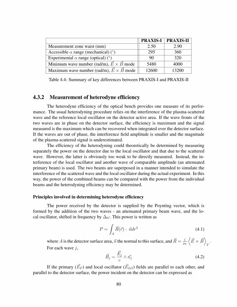
PRAXIS-I PRAXIS-IIMeasurement zone waist (mm) 2.50 2.90Accessible α range (mechanical) () 295 360Experimental α range (optical) () 90 320Minimum wave number (rad/m), ~E × ~B mode 5480 4000Maximum wave number (rad/m), ~E × ~B mode 12600 13200
Table 4.4: Summary of key differences between PRAXIS-I and PRAXIS-II
4.3.2 Measurement of heterodyne efficiencyThe heterodyne efficiency of the optical bench provides one measure of its perfor-
mance. The usual heterodyning procedure relies on the interference of the plasma-scatteredwave and the reference local oscillator on the detector active area. If the wave fronts of thetwo waves are in phase on the detector surface, the efficiency is maximum and the signalmeasured is the maximum which can be recovered when integrated over the detector surface.If the waves are out of phase, the interference field amplitude is smaller and the magnitudeof the plasma-scattered signal is underestimated.
The efficiency of the heterodyning could theoretically be determined by measuringseparately the power on the detector due to the local oscillator and that due to the scatteredwave. However, the latter is obviously too weak to be directly measured. Instead, the in-terference of the local oscillator and another wave of comparable amplitude (an attenuatedprimary beam) is used. The two beams are superposed in a manner intended to simulate theinterference of the scattered wave and the local oscillator during the actual experiment. In thisway, the power of the combined beams can be compared with the power from the individualbeams and the heterodyning efficiency may be determined.
Principles involved in determining heterodyne efficiency
The power received by the detector is supplied by the Poynting vector, which isformed by the addition of the two waves - an attenuated primary beam wave, and the lo-cal oscillator, shifted in frequency by ∆ω. This power is written as
P =
∫A
~R(~r) · ~ndr2 (4.1)
whereA is the detector surface area, ~n the normal to this surface, and ~R = 1µ0
⟨~E × ~B
⟩T.
For each wave j,
~Bj =~Ejc∧ ~nj (4.2)
If the primary ( ~EP ) and local oscillator ( ~ELO) fields are parallel to each other, andparallel to the detector surface, the power incident on the detector can be expressed as
80
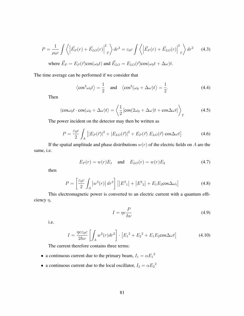
P =1
µ0c
∫ ⟨∣∣∣ ~EP (r) + ~ELO(r)∣∣∣2T
⟩dr2 = ε0c
∫ ⟨∣∣∣ ~EP (r) + ~ELO(r)∣∣∣2T
⟩dr2 (4.3)
where ~EP = EP (~r)cos(ω0t) and ~ELO = ELO(~r)cos(ω0t+ ∆ω)t.
The time average can be performed if we consider that⟨cos2ω0t
⟩=
1
2and
⟨cos2(ω0 + ∆ω)t
⟩=
1
2. (4.4)
Then
〈cosω0t · cos(ω0 + ∆ω)t〉 =
⟨1
2[cos(2ω0 + ∆ω)t+ cos∆ωt]
⟩T
(4.5)
The power incident on the detector may then be written as
P =ε0c
2
∫A
[|EP (~r)|2 + |ELO(~r)|2 + EP (~r) ELO(~r) cos∆ωt
](4.6)
If the spatial amplitude and phase distributions w(r) of the electric fields on A are thesame, i.e.
EP (r) = w(r)E1 and ELO(r) = w(r)E2 (4.7)
then
P =
[ε0c
2
∫A
∣∣w2(r)∣∣ dr2
] [∣∣E21
∣∣+∣∣E2
2
∣∣+ E1E2cos∆ωt]
(4.8)
This electromagnetic power is converted to an electric current with a quantum effi-ciency η,
I = ηeP
hν(4.9)
i.e.
I =ηeε0c
2hν
[∫A
w2(r)dr2
]·[E1
2 + E22 + E1E2cos∆ωt
](4.10)
The current therefore contains three terms:
• a continuous current due to the primary beam, I1 = αE12
• a continuous current due to the local oscillator, I2 = αE22
81
• an alternating current at the frequency ∆ω, I∆ω = αE1E2
with α = ηeε0c2hν
∫Aw2(r)dr2, i.e.
I∆ω =√I1I2
The alternating current is measured in the form of an electric power Pe entering anamplifier of gain G with a resistance Ri of 50Ω,
Pe =1
2RiI∆ω
2 (4.11)
The total electric power leaving this amplifier is
Ps =G
2RiI∆ω
2 (4.12)
If the detector heterodyne efficiency is ideal, as in the calculation above, then the ratiobetween the local oscillator current at the frequency ∆ω and the continuous currents I2 andI1 is such that
I∆ω2
I1I2
= 1 (4.13)
or
2PsGRiI1I2
= 1 (4.14)
The actual system is not perfect; the profiles w(r) of the primary and local oscillatorbeams are not the same because the beams are not strictly parallel. Hence the resultingdistribution of phases on the detector surface is not the same. The heterodyne efficiency ηHis defined as the ratio between the power of the oscillator at the frequency ∆ω, measured atthe exit of the preamplifier (Pm), and the power which is expected from the oscillator if thelocal oscillator and primary beam electric fields were identical, i.e.
ηH =PmPs
=2Pm
GRiI1I2
(4.15)
Heterodyning efficiency experiment
Fig. 4.3 shows the setup used for determining the heterodyne efficiency.Mirrors are denoted by M , full (100%) absorbers by A, partial absorbers by a, lenses
with L, and beam-splitters by BS. The reflectances of BS1 and BS2 are 0.44% and 58%respectively. The partial absorbers a1, a2, a3 and a4 are CaF2 windows of thicknesses 3.5, 5,6 and 3.5 mm respectively, with corresponding transmittances of 28%, 17%, 12% and 28%.The primary beam P (in red) and local oscillator LO (in blue) are first superposed at BS2,and the superposition of the beams is maintained over a long distance (6.7 m, on the orderof the distance between the translator-rotator and the detector in the plasma experiments)
82

Figure 4.3: Schematic of optical bench setup for determination of heterodyning efficiency
up to the detector, with a detector beam size comparable to that used during the plasmaexperiments.
The primary beam has an initial power of 35 W; after partial reflection and attenuationby the absorbers, it provides a detector current of 0.243 mA. The local oscillator is reflectedby BS2 and further attenuated by a4; with a reference 5 dB attenuation in the 40 MHz AODsource, it provides a detector current of 0.221 mA. The detector current, when both beamsare allowed to arrive at the detector, is 0.432 mA. The thermal noise current present when thedetector is closed is 0.029 mA and is subtracted from the beam currents.
The 40 MHz peak, which is seen on the detector and pre-amplifier output, correspondsto the oscillation at the frequency ∆ω mentioned above. It has a level of 8.10 dBm, i.e. Pm =6.46 mW. The preamplifier gain G has been independently measured as 37.22 ± 0.1 dBm.
Substituting these values into Eq. 4.15,
ηH = 1.19± 2% (4.16)
This value is close to, but slightly larger than, 1; this is most likely due to slightlaser power variations or a slight error in the determination of the preamplifier gain. Theheterodyning efficiency of the bench is maximum, which means that the wavefronts alongthe plasma-scattered field optical path are indeed in phase with those of the local oscillator.Hence no losses in the measured signal are due to the heterodyning procedure.
4.3.3 Verification of signal levelNow that it has been assured that the heterodyning efficiency is good, the signal level
output by the bench may be verified. This is done by measuring the density fluctuation of a
83

signal of known amplitude using the bench and comparing this measured signal level to itsexpected theoretical level. This calibration may be most easily done using a piezo-electrictransducer which excites an acoustic wave.
The bench and off-bench assemblies are set up as for the plasma experiments, withthe piezo placed in the position which would normally be occupied by the thruster, with thebeams crossing just in front of the transducer face. Fig. 4.4 shows the simplified setup formeasurements using an acoustic wave.
Figure 4.4: Orientation of ~k for calibration using an acoustic wave. The acoustic wave vectoris denoted by ~ka, the observation wave vector by ~k
The observation wave vector ~k adjusted such that it is oriented in approximately thesame direction and parallel to the acoustic wave vector ~ka, and the scattering angle is first setto an arbitrary value of around 13 mrad. The corresponding frequency f at which a soundwave propagating in air at a velocity of cs would be detected is related to the wave number kby
f =csk
2π(4.17)
The value of cs used is 340 m/s. The transducer is supplied with a sine wave signal(amplitude 2.4 V) via a signal generator, with a frequency close to f . The frequency of thesine wave is then more finely-tuned until the observed scattered signal reaches a peak asobserved on a spectrum analyser, at 422 kHz in this case. This frequency is then maintainedand used to make finer adjustments of the magnitude of the wave vector. The orientation ofthe transducer is adjusted to ensure that the acoustic wave vector is parallel to ~k; providedthis is the case, the signal is maximum.
84

The displacement characteristic of this transducer is 4.8×10⁻¹⁰ m/V, known with anaccuracy of 50% [59]. For the supplied sine wave of frequency, the corresponding displace-ment amplitude, a, is 11.5×10⁻¹⁰ m.
The amplitude of this signal, n1, is given by
n1
n0
=aω
cs(4.18)
where n0 is the density of air (2.68×1025 molecules/m3) and ω the acoustic wavefrequency.
The mean squared value of this amplitude is
⟨n1
2⟩
=1
2
(aωn0
cs
)2
(4.19)
Using the above numerical values, 〈n12〉 = 2.89×1040 m−6.
Hence the r.m.s value of the density fluctuation of the excited acoustic wave,√〈n1
2〉,is 1.70×10²⁰±50% m−3. For a plane harmonic wave, the r.m.s value of the measured densityfluctuation, 〈na2〉, may be obtained from the optical bench characteristics and measurementsas
⟨na
2⟩
=2
(rRλL)2
hν
ηPo
⟨i(t)2⟩⟨Iph(ω)2⟩ (4.20)
where⟨i(t)2⟩ is the signal mean square value and
⟨Iph(ω)2⟩ the spectral density of
the photonic noise. rR is the Rayleigh radius, L the length of the scattering volume (definedhere by the transducer diameter, 25 mm). The primary beam power Pp is 35 W.
The spectral density of the photonic noise at the pre-amplifier output is obtained bysubtracting the spectral density at a reference frequency, obtained when the detector is closed(PDC), from that obtained when the laser beam is incident on the detector, but the piezoinactive (PDO). PDC = -91 dBm, or 7.94×10⁻¹⁰ mW, while PDO = -98 dBm, or 1.58×10⁻¹⁰
mW.The photonic noise spectral density is written
⟨Iph(ω)2⟩ =
dPph(ω)
df(4.21)
where dPph(ω) is PDC - PDO and df the bandwidth used, 10 kHz. dPph(ω) is 6.36×10⁻¹³
W. Hence the spectral density of the photonic noise is 6.36×10⁻¹⁷ W/Hz.Now, the signal power is obtained from the level of the 422 kHz peak, which is -16.60
dBm, or 2.19×10⁻⁵ W. Hence ⟨i(t)2⟩⟨Iph(ω)2⟩ = 3.44× 10¹¹ Hz (4.22)
Substituting this ratio into Eq. 4.20, we obtain
85

⟨na
2⟩
= 2.77× 1040 m−6 (4.23)
Therefore√〈na2〉 = 1.66× 10²⁰ m−3.
This value is very close to that predicted for√〈na2〉. This indicates that the sig-
nal level measured using the bench is indeed representative of the true level of the densityfluctuations.
The experiments described in this chapter, aimed at measuring the heterodyning effi-ciency and verifying the signal level, have revealed that the signal level output by the benchis not subject to important losses or underestimations. This will allow the density fluctuationlevel to be interpreted later on with greater confidence.
86

Chapter 5
Phase II experiments: mode localization
Contents5.1 Mode localization . . . . . . . . . . . . . . . . . . . . . . . . . . . . . . 87
5.1.1 Positioning of observation volume centre . . . . . . . . . . . . . . 88
5.2 Physical hypotheses concerning the localization of the ~E × ~B mode . . . 94
5.1 Phase II experiments: Localization of the ~E × ~B modealong z
THe negative frequency peaks in the observed signal spectra are consistent with fluctua-tions propagating at a phase velocity opposed in sign to the wave vector. In Part I, two
explanations were proposed for the presence of these peaks: (i) the negative frequency modemay correspond to a measurement of the fluctuation in the 03h00 side of the thruster channel,in which case the relative peak magnitudes are due to differing sensitivities due to the place-ment of the observation lozenge along z, or (ii) fluctuations are propagating in the directionof Vd and anti-Vd in the same thruster channel side.
The negative peak amplitudes during the first phase of experiments were consistentlyseveral orders smaller than the positive peak amplitudes. This could have resulted from theplacement of the observation volume, or a difference in the fluctuation intensity in the az-imuthal direction.
An experiment to check the origin of negative peak frequencies and different peakamplitudes is performed during the second phase of experiments and is described in thischapter.
87

5.1.1 Positioning of observation volume centreThe positioning of the observation volume centre depends on the manner of beam
convergence in front of the thruster exit plane. Prior to each experiment, the convergencezone of the primary and local oscillator beams is simulated outside the vacuum chamber, asdescribed in Chapter 2. The superposition of each beam is checked by a systematic compari-son and adjustment of the beam positions, but some error is inherent in the procedure.
Fig. 5.1(a) shows an error in the superposition of the two laser beams (primary, inred, local oscillator, in blue) in the xOy plane. The typical error involved in such positioning,dy, is on the order of 0.5 mm, and translates to an error in the positioning of the measurementzone (in light blue), shown in an exaggerated view in Fig. 5.1(b).
Figure 5.1: Error in positioning of the measurement volume resulting from an imperfectsuperposition of the primary and local oscillator beams in the plane xOy. (a) shows thesituation in the xOy plane and (b) the yOz plane, for an exaggerated superposition error
The corresponding error dz in the horizontal positioning of the volume, is
dz =dy
θe(5.1)
In the present localization experiment, θe = 17.5 mrad, giving a dz value of about 3cm. This value for θe was chosen as a compromise; for small angles, since the correspondingobservation volume has a long extension along z it becomes difficult to focus the convergenceregion on just one side of the thruster at once. On the other hand, the signal intensity has beenseen to drop exponentially as θe increases, and the frequency peaks become noisier. At 17.5mrad, the maximum signal intensity is already two orders of magnitude smaller than thatwhich could be obtained at the smallest angles. The observation wave vector is orientedparallel to the ~E × ~B direction and the observation volume is located 13.5 mm from thethruster exit plane.
In this experiment, the measurement volume is shifted along z to seven different posi-tions, from−30 to +30 cm with respect to the thruster axis. This shift in position is performedby means of an adjustment on the optical bench of the virtual intersection position for the two
88

beams. This adjustment is made by changing the orientation of the mirror M13, which is theobject-focus of the lens L5, with the scattering angle remaining unchanged.
The resulting spectra obtained at the different positions show two peaks (of positiveand negative frequency) whose amplitudes change as a function of the position of the mea-surement volume along z. The positive and negative peak intensities are determined at eachposition. The results are shown in Fig. 5.2, where the positive peak intensities are shown inblue, the negative peak intensities in red.
-30 -20 -10 0 10 20 300
500
1000
1500
2000
S(k)
Distance along z from thruster origin (cm)
Figure 5.2: Positive (in blue) and negative (in red) frequency peak intensities as a function ofthe beam intersection position along z
Fig. 5.2 shows that the peak intensities are indeed linked to the position along z.The positive peak dominates when the convergence volume is situated preferentially on the09h00 side of the thruster, while the negative peak dominates when the volume is shiftedto the 03h00 side of the thruster. This first observation confirms that the large difference inpositive and negative frequency peak intensities discussed in Part I is due (mainly) to theplacement of the observation zone.
The evolution of the peak intensity as a function of position may be studied by con-sidering the intensity which would be measured if the observation volume were centered ata position ~r0. We assume that the mode has a point source of intensity I±, situated at ~r±, asdepicted in Fig. 5.3.
In this case, the measured intensity I(~r0) is of the form
I(~r0) =
∫ ∫ ∫u(~r − ~r0)2I±δ(~r±)d3~r (5.2)
89
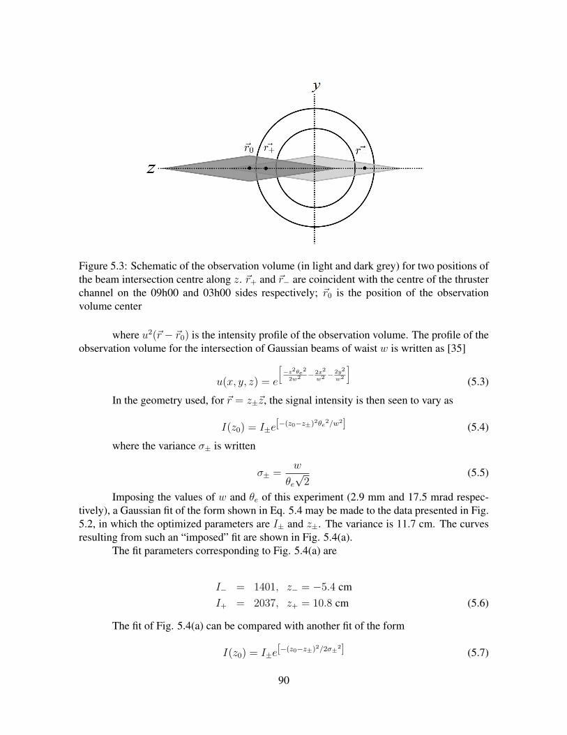
Figure 5.3: Schematic of the observation volume (in light and dark grey) for two positions ofthe beam intersection centre along z. ~r+ and ~r− are coincident with the centre of the thrusterchannel on the 09h00 and 03h00 sides respectively; ~r0 is the position of the observationvolume center
where u2(~r − ~r0) is the intensity profile of the observation volume. The profile of theobservation volume for the intersection of Gaussian beams of waist w is written as [35]
u(x, y, z) = e
[−z2θe2
2w2 − 2x2
w2 −2y2
w2
](5.3)
In the geometry used, for ~r = z±~z, the signal intensity is then seen to vary as
I(z0) = I±e[−(z0−z±)2θe
2/w2] (5.4)
where the variance σ± is written
σ± =w
θe√
2(5.5)
Imposing the values of w and θe of this experiment (2.9 mm and 17.5 mrad respec-tively), a Gaussian fit of the form shown in Eq. 5.4 may be made to the data presented in Fig.5.2, in which the optimized parameters are I± and z±. The variance is 11.7 cm. The curvesresulting from such an “imposed” fit are shown in Fig. 5.4(a).
The fit parameters corresponding to Fig. 5.4(a) are
I− = 1401, z− = −5.4 cmI+ = 2037, z+ = 10.8 cm (5.6)
The fit of Fig. 5.4(a) can be compared with another fit of the form
I(z0) = I±e[−(z0−z±)2/2σ±2] (5.7)
90
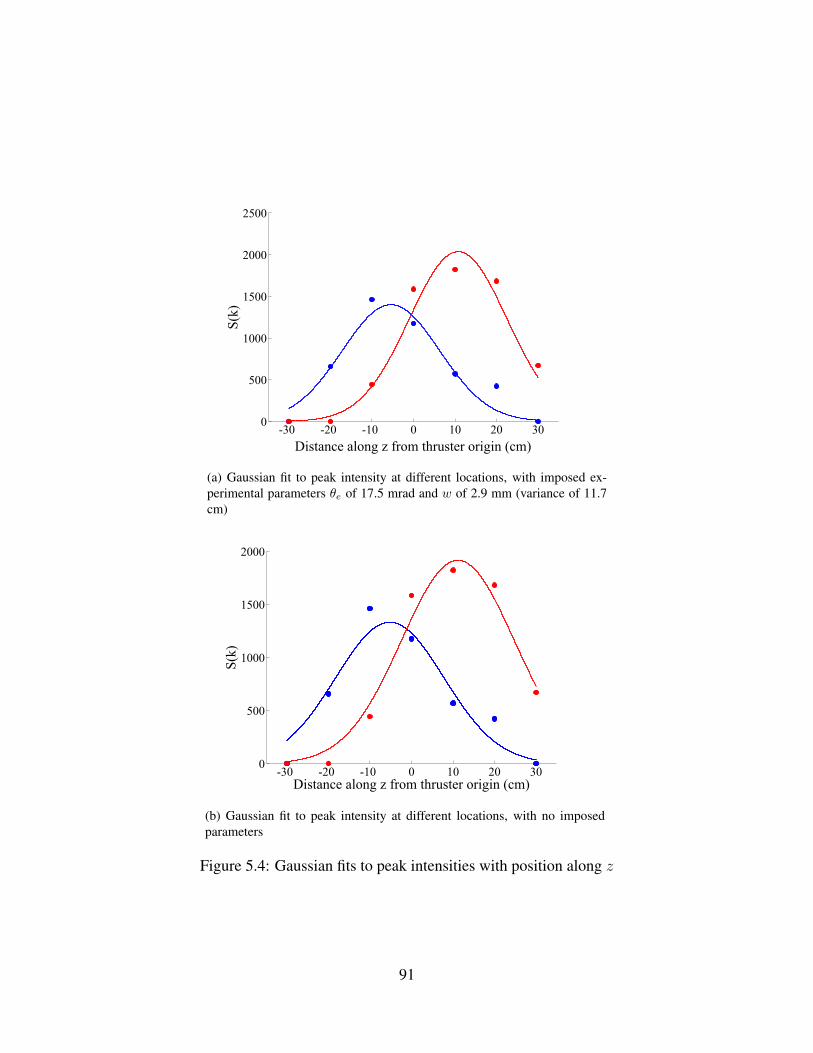
-30 -20 -10 0 10 20 300
500
1000
1500
2000
2500
S(k)
Distance along z from thruster origin (cm)
(a) Gaussian fit to peak intensity at different locations, with imposed ex-perimental parameters θe of 17.5 mrad and w of 2.9 mm (variance of 11.7cm)
-30 -20 -10 0 10 20 300
500
1000
1500
2000
S(k)
Distance along z from thruster origin (cm)
(b) Gaussian fit to peak intensity at different locations, with no imposedparameters
Figure 5.4: Gaussian fits to peak intensities with position along z
91

for which the experimental parameters are no longer directly imposed. I± and σare optimized. The resulting “free” fit is shown in Fig. 5.4(b) and the corresponding fitparameters are
I− = 1331, z− = −5.2 cm, σ− = 13.1 cmI+ = 1916, z+ = 11.2 cm, σ+ = 13.6 cm (5.8)
Certain conclusions may be drawn from these fits.For the imposed fit, the maxima of the positive and negative frequency peaks are
separated by 16.2 cm; this separation is larger than the separation of the centre points of thechannels, which is only 12.5 cm. This indicates that the fluctuations are most likely situatedat the exterior of the thruster channel, near the outer wall. For the free fit, the maxima arespaced by 16.4 cm, providing confirmation of the observation made using the imposed fit.
For both fits, the z = 0 position does not coincide with the thruster origin. The z = 0position is situated at 2.7 cm for the imposed fit, and at 3.0 cm for the free fit, on the order ofthe positioning error which appears during the alignment.
The standard deviation for the imposed fit, σ±, is 11.7 cm. This value is somewhatsmaller than σ+ and σ− obtained from the free fit.
The main contribution to the amplitude of the positive and negative peak amplitudes isevidently the positioning of the thruster volume along z. However, there is also a possibilitythat a part of the measured mode intensity, for example, of the negative frequency peak, isdue to not only to fluctuations in the 03h00, but also to backwards-propagating (opposed tothe drift velocity vector) fluctuations located in the 09h00 side of the thruster channel. Thisscenario is not the dominant one, but may arise due to a partial reflection of the main modein the 09h00 side.
How can such an effect be identified? The shape of the experimental points of thepositive frequency peak intensities in Fig. 5.2 is one reason to suspect that there might be acontribution of a reflected wave from the 03h00 side of the thruster channel: the right flankis tail-like and non-symmetric with the left flank. A possible better fit to this data is the sumof two Gaussians centered at different locations.
For the positive frequency peak, the new fit may be thus written as
I+(z0) = I+ae[−(z0−z+)2/2σ2] + I+be
[−(z0−z−)2/2σ2], (5.9)
a form which now includes a term containing the possible intensity contribution dueto propagations in the 03h00 side, I+be
[−(z0−z−)2/2σ2]. Similarly, for the negative frequencypeak, the new fit may be written as
I−(z0) = I−ae[−(z0−z−)2/2σ2] + I−be
[−(z0−z+)2/2σ2], (5.10)
The forms shown in Eq. 5.9 and Eq. 5.10 will be referred to as “mixed” fits. Thefirst terms in both equations will be referred to as the “principal” Gaussian, the second as the“secondary” Gaussian.
92
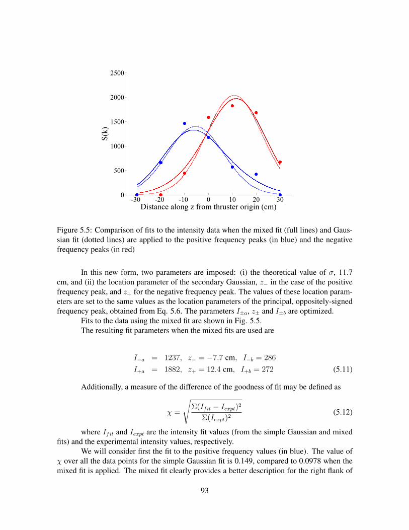
-30 -20 -10 0 10 20 300
500
1000
1500
2000
2500
S(k)
Distance along z from thruster origin (cm)
Figure 5.5: Comparison of fits to the intensity data when the mixed fit (full lines) and Gaus-sian fit (dotted lines) are applied to the positive frequency peaks (in blue) and the negativefrequency peaks (in red)
In this new form, two parameters are imposed: (i) the theoretical value of σ, 11.7cm, and (ii) the location parameter of the secondary Gaussian, z− in the case of the positivefrequency peak, and z+ for the negative frequency peak. The values of these location param-eters are set to the same values as the location parameters of the principal, oppositely-signedfrequency peak, obtained from Eq. 5.6. The parameters I±a, z± and I±b are optimized.
Fits to the data using the mixed fit are shown in Fig. 5.5.The resulting fit parameters when the mixed fits are used are
I−a = 1237, z− = −7.7 cm, I−b = 286
I+a = 1882, z+ = 12.4 cm, I+b = 272 (5.11)
Additionally, a measure of the difference of the goodness of fit may be defined as
χ =
√Σ(Ifit − Iexpt)2
Σ(Iexpt)2(5.12)
where Ifit and Iexpt are the intensity fit values (from the simple Gaussian and mixedfits) and the experimental intensity values, respectively.
We will consider first the fit to the positive frequency values (in blue). The value ofχ over all the data points for the simple Gaussian fit is 0.149, compared to 0.0978 when themixed fit is applied. The mixed fit clearly provides a better description for the right flank of
93

the experimental values of the positive frequency peak. In the case of the negative frequencypeak, the value of χ for the simple Gaussian is 0.120, and 0.101 for the mixed case.
These observations indicate that the hypothesis of partial reflection of the modes is abetter estimate of the experimental observations. The mixed fit is a good means of estimatingthe contribution to the measured signal of fluctuations in the opposite channel. The param-eters obtained from the fit can be used to estimate the percentage of energy which is due tofluctuations in the opposite channel.
This rate, τR, is defined as
τR =I∓bI±a
(5.13)
i.e. this rate is determined through a comparison of the amplitude of the secondaryGaussian (obtained from the mixed fit) to the amplitude of the principal Gaussian due to theoppositely-signed frequency peak.
Hence τR for the positive frequency peak is 15%, i.e. 15% of the positive peak energyis due to a reflection of the wave propagating in the opposite channel. The reflection rate forthe negative frequency peak is 22%.
This reflection sets up standing waves. The periodicity of the standing wave amplitudeis half the propagating wavelength. Our observation on the form factor distribution withlength scale shows that the largest fluctuation amplitude occurs at wavelengths equal to, orlonger than, 1.6 mm. Thus the observed standing wave energy periodicity is equal to, orlonger than, 0.8 mm. These waves might account for the presence of the periodic erosionpattern which appears on the thruster ceramic; in particular, the periodicity of these groovesis on the order of a 1 or 2 mm. There is a possibility that the modes we observe near theselength scales play some role in the erosion.
This is a point which underscores the usefulness of the thruster plasma experimentswhich can be performed using collective light scattering: apart from enabling the study ofa variety of instabilities, it is also possible to identify the source of other phenomena whichaffect thruster performance and lifetime.
5.2 Physical hypotheses concerning the localization of the~E × ~B mode
The observations on the localization of the ~E × ~B mode along z1 may be explainedin terms of possible physical mechanisms which are at the origin of the instability. The mostintense modes are likely to be located on the periphery of the outer ceramic, rather than nearthe centre of the thruster channel. This scenario can be explained by considering the radialdistribution of the magnetic and electric fields.
The electron cyclotron drift length, lce, is written as
lce =2πmeE
qeB2(5.14)
94

Figure 5.6: Variation of electron cyclotron drift length lce with radial position (left) and aschematic of wavefront deformation in the direction of propagation (right)
This length scale corresponds to the length scale of the instability, on the order of amm. lce evolves with the radial position as shown qualitatively in Fig. 5.6.
lce is maximum near the outer channel and smaller near the interior; this non-uniformitywould generally mean that no particular length scale of instability, and hence no particularmode, is favoured to develop. If, however, the value of lce were maintained over a sufficientradial distance, a particular mode could grow, mainly parallel to ~E× ~B. This mode propagatesfrom a region where the wavefront is aligned with the thruster radius. As the wavefront movesazimuthally, the distance of the wavefront to the previous, 2π-delayed front, is shorter on theinner and outer locations of the thruster channel where lce is shorter. Thus the wavefront isbent to a convex shape. The local wave vector, normal to this surface, is oriented outwardsat the major channel radius, and inwards at the minor radius, as depicted in Fig. 5.6. Themain direction of propagation diverges from the ~E × ~B direction and this could account forthe observation of the most intense modes near the outer channel wall. The divergence fromthe ~E × ~B direction will be revisited in Chapter 6.
The experiments described in this chapter have been successfully used to account forthe negative frequency peak seen on typical ~E× ~B spectra, through a localization of the mode
95

along z. The possibility of reflected modes and the consequences on the peak intensity havealso been considered. Additional aspects concerning the nature of the mode propagation willbe considered in the next chapter.
96

Chapter 6
Phase II experiments: low wave numbercharacteristics and mode directionality
Contents6.1 Mode energy saturation at low wave numbers . . . . . . . . . . . . . . . 98
6.2 Form factor variation in the (kx, kθ) plane . . . . . . . . . . . . . . . . 100
6.2.1 ~E × ~B mode directionality in the (kx, kθ) plane . . . . . . . . . . . 100
6.2.2 Axial mode directionality in the (kx, kθ) plane . . . . . . . . . . . 104
6.3 Mode frequency variation in the (kx, kθ) plane . . . . . . . . . . . . . . 105
6.3.1 Frequency variation with α for the ~E × ~B mode . . . . . . . . . . 105
6.3.2 Frequency variation with α for the axial mode . . . . . . . . . . . . 106
6.4 Form factor variation in the (kx, kr) plane . . . . . . . . . . . . . . . . 107
6.4.1 Comparison of fluctuations perpendicular and parallel to ~B . . . . . 107
6.4.2 The “cathode” mode . . . . . . . . . . . . . . . . . . . . . . . . . 109
6.4.3 Axial mode width and mean angle in the (kx, kr) plane . . . . . . . 110
6.5 Mode frequency variation in the (kx, kr) plane . . . . . . . . . . . . . . 111
6.6 Form factor variation in the (kθ, kr) plane . . . . . . . . . . . . . . . . . 113
6.6.1 ~E × ~B mode directionality in the (kθ, kr) plane . . . . . . . . . . . 116
6.6.2 Axial mode directionality in the (kθ, kr) plane . . . . . . . . . . . . 117
6.7 Mode frequency variation in the (kθ, kr) plane . . . . . . . . . . . . . . 119
6.7.1 Frequency variation with β for the ~E × ~B mode . . . . . . . . . . 119
6.7.2 Frequency variation with β for the axial mode . . . . . . . . . . . . 119
6.8 Form factor of the ~E × ~B at three reference values of β with varying α 120
6.9 Frequency of the ~E × ~B at three reference values of β with varying α . 121
6.10 Visualization of mode directionalities . . . . . . . . . . . . . . . . . . . 121
97
6.10.1 ~E × ~B directionality . . . . . . . . . . . . . . . . . . . . . . . . . 122
6.10.2 Axial mode directionality . . . . . . . . . . . . . . . . . . . . . . 122
6.11 Physical hypotheses concerning the directionality of the ~E × ~B mode . 125
6.12 Redetermination of the density fluctuation rate . . . . . . . . . . . . . . 126
6.1 Mode energy saturation at low wave numbers
AN experiment is performed in which the dispersion relation and form factor evolutionwith wave number for the ~E × ~B mode are determined. The goals of this experiment in
Phase II are to confirm the characteristics of the previously observed dispersion relation, andalso examine the behaviour of the ~E × ~B mode at the longer length scales which are nowachievable.
The magnitude of the wave vector is systematically varied between 4000 and 12600rad/m, while the orientation of the wave vector is maintained parallel to the ~E × ~B direction(α = 90). The experiment is performed with a flow rate of 18 mg/s and the beams arepositioned at a distance of 12 mm from the thruster exit plane, a location chosen to providethe maximum signal level, as based on observations in the Phase I experiments.
The first unstable mode predicted by linear theory appears for kyVd/ωce = 1. Thecorresponding value of ky associated with this mode is 3956 rad/m, as was shown in Part I.The minimum value of 4000 rad/m attainable by PRAXIS-II is very close to this value, butan exploration below this value requires a number of modifications to the bench which arebeyond the scope of the present experimental campaign.
The dispersion relation for the given experimental conditions is shown in Fig. 6.1.The group velocity is 4.21×10³ m/s and the y-intercept -17.9 kHz, not significantly differentfrom zero.
Of more interest is the trend in form factor, shown in Fig. 6.2. The e-decrement inFig. 6.2 is 0.5 mm.
Surprisingly, the form factor does not show the marked slope change at large wavenumber which was shown in Part I. The reason for this inconsistency is not yet clear. The formfactor exhibits an exponential dependence on wave number. At the smallest wavenumbers,there is no evidence that the energy of the mode has reached its maximum value, and itmay very well continue to increase as the wave number decreases. A saturation in the modeamplitude at the first cyclotron harmonic can therefore not be confirmed at present.
In order to describe azimuthally-propagating fluctuations, poloidal coordinates willbe adopted in this chapter. Fig. 6.3 shows the configuration which will be used to describethe experiments in this chapter. The laser beam crosses the thruster axis along z1. The wavevector is oriented at an angle α to the direction x1, and has components kθ and kx of variablemagnitudes. kθ is oriented in the opposite direction to the electron drift velocity, while kx is
98

0 2000 4000 6000 8000 10000 120000
2
4
6
8
10
12x 10
6
Frequency (Hz)
k (rad.m-1)
Figure 6.1: Dispersion relation for the ~E× ~B mode, for an experiment featuring the minimumwave number
0 2000 4000 6000 8000 10000 12000 140006
7
8
9
10
11
loge[S(k)]
k (rad.m-1)
Figure 6.2: Form factor variation with wave number, for an experiment featuring the mini-mum wave number
99

in the direction of the electric field. kr is oriented in the opposite direction to the magneticfield. In the orientation shown in Fig. 6.3, the kr component of the wave vector is zero.
Figure 6.3: Poloidal coordinate system for the examination of the kθ and kx components ofthe wave vector when the laser beam crosses the thruster axis along z1; (a) shows a side viewof the thruster with the reference angle α, which is varied, (b) shows the orientation of thewave vector components as viewed from the thruster face
6.2 Form factor variation in the (kx, kθ) planeThe variation of the mean square amplitude of the modes can be examined on PRAXIS-
II over an expanded range of 320.In these experiments, the magnitude of the wave vector is fixed at the lower end of
the range of accessible wave numbers, for two reasons: firstly, to allow a large signal to beobtained and to study its progressive change in level over a sufficiently large range of angles,and secondly, to also allow a visualization of the high frequency axial mode within the 20MHz frequency range of the experiment.
In the experiment presented here, the gas flow rate is 18 mg/s, and the observationvolume is 17 mm from the thruster exit plane. The wave number used is 5928 rad/m.
6.2.1 ~E × ~B mode directionality in the (kx, kθ) planeFig. 6.4 shows the form factor variation with α, for the positive and frequency peaks.
The ~E × ~B drift direction corresponds to 90.
100

70 80 90 100 110 120 130 1400
2
4
6
8
10
12x 10
4
S(k)
Alpha (°)
Figure 6.4: Variation of form factor of the ~E × ~B mode with α in the (kx, kθ) plane. Thepositive frequency peak data is shown in blue, the negative frequency peak data in red
The difference in amplitudes of the peaks is due to the positioning of the observationvolume along the direction z1, as has been shown earlier.
The data points are fitted with Gaussian curves whose parameters are
A1 = 1.04× 10⁵, µ1 = 106.8, σ1 = 5.60
A2 = 1.54× 10⁴, µ2 = 85.7, σ2 = 7.05 (6.1)
with
µ1 − µ2 = 21.1
µ = (µ1 + µ2)/2 = 96.25 (6.2)
where A, µ and σ represent the amplitude, mean value and standard deviation forGaussian fits to the positive frequency peak data (subscript 1) and the negative frequencypeak data (subscript 2).
The first important observation from this experiment is that the maximum in energyof the mode is not obtained at an α of 90 for the positive frequency peak (or 90 for thenegative frequency peak), as was expected. From the values in Eq. 6.1, it is evident thatthe mode does not propagate purely parallel to ~E × ~B, but with an additional inclination of16.8 towards the thruster for the positive peak, and 4.3 towards the thruster for the negativepeak. The reference angle α is not absolute, however, the precision in the determination ofthe wave vector orientation in the (kx, kθ) plane is 2.7±4. The angular position of the twopeaks should be symmetric on either side of the ~E × ~B drift direction; this is obtained if the
101

reference angle is shifted by (µ1+µ2
2− 90), or 6.25. This is an acceptable shift, in the range
of precision of the measurements. For the symmetric positive and negative frequency peaks,the mean deviation from the ~E × ~B drift direction is therefore 10.6.
The second important observation is that the mean angular width σ of the mode isonly 6.33 (σ1+σ2
2). In the experiments with PRAXIS-I, the angular opening of the mode in
the x1O1y1 quadrant was greatly overestimated at 45. In reality, the mode has a much morelimited angular extension in this plane, so small, in fact, that it must be considered in thecontext of the resolution of the diagnostic in order to determine its true extent.
The relation of the angular device resolution σd to the wave number k and devicewave number resolution is shown in Fig. 6.5.
Figure 6.5: Relation between device angular resolution σd and wave number resolution ∆k
Its r.m.s value is
σd =
√2
2πkw· 360 (6.3)
The device resolution is 4.71. A Gaussian with standard deviation of σd and with anamplitude and mean value chosen to be equivalent to the positive frequency peak values isnow compared to the experimental data (Fig. 6.6).
The observed angular extension of the mode is broadened by the device resolution; ifthis effect is excluded, then the true extension of the mode σ is
σ =√σ1
2 − σd2 (6.4)
The true angular extension of the mode in this plane is therefore 3.0.It should be noted that when ~k is oriented parallel to ~E × ~B, but in the opposite
direction to the drift, as is the case when α is around 270, near-identical observations aremade: the only difference is that the negative frequency peak is now the dominant peak (Fig.6.7).
The Gaussian fit parameters for this symmetric position of ~k are shown in Eq. 6.5.
102

70 80 90 100 110 1200
2
4
6
8
10
12x 10
4
S(k)
Alpha (°)
Figure 6.6: Comparison of experimental angular extension of the ~E× ~B mode in the (kx, kθ)plane for the positive frequency peak (in blue) to the natural angular extension resulting fromthe device resolution (dotted line)
220 230 240 250 260 270 280 290 3000
2
4
6
8
10
12x 10
4
S(k)
Alpha (°)
Figure 6.7: Variation of form factor of the ~E × ~B mode with α in the (kx, kθ) plane. Thepositive frequency peak data is shown in blue, the negative frequency peak data in red
103
A1 = 6.35× 10³, µ1 = 254.6, σ1 = 7.05
A2 = 1.00× 10⁵, µ2 = 276.0, σ2 = 6.24 (6.5)
with
µ1 − µ2 = 21.4
µ = (µ1 + µ2)/2 = 265.3 (6.6)
The difference in mean angular positions in Eq. 6.6 is the same as in Eq. 6.2 to within0.3. The difference in the mean angle µ, obtained when the wave vector is oriented at 90
and 270, is not precisely 180, but 169. This indicates a slight irregularity in the mirrorrotation used.
In summary,
• the ~E × ~B mode propagates within a very narrow angular range in the (kx, kθ) plane,determined to be 3.0
• the mode is inclined at 10.6 angle to the vertical, oriented inwards towards the thrusterexit plane, and therefore possesses a component anti-parallel to the electric field
The observation that the mode is not aligned purely along the ~E × ~B drift directionbut is directed towards the interior of the thruster has certain consequences which will beexamined more closely in future work. For instance, it has already been demonstrated thatstanding waves can be set up in the thruster which could contribute to the periodic erosionpattern of the ceramic. The inclination of the mode toward the interior would appear to makesuch erosion likely.
6.2.2 Axial mode directionality in the (kx, kθ) planeThe angular extension of the axial mode is studied in the same experiment, albeit at a
slightly different wave number, 5631 rad/m. The variation of the form factor of the positivehigh frequency peak with α (observed when ~k is oriented in about the same direction as theion beam) is shown in Fig. 6.8.
The Gaussian fit parameters corresponding to Fig. 6.8 are
A = 4.37× 10³, µ = 8.22, σ = 24.2 (6.7)
The first important observation here is that the angular extension of the axial mode inthe (kx, kθ) plane is much greater than that of the ~E × ~B mode. After removing the effect ofthe device resolution from the peak width, the angular extension of the mode is 23.7.
The mean angle is not aligned with the x1 direction, with a deviation of 8 whichexceeds the angular resolution. This non-zero angle with respect to x1 appears to correspondwith visual observations which show that the thruster plume is not entirely symmetric aboutthe thruster axis.
104
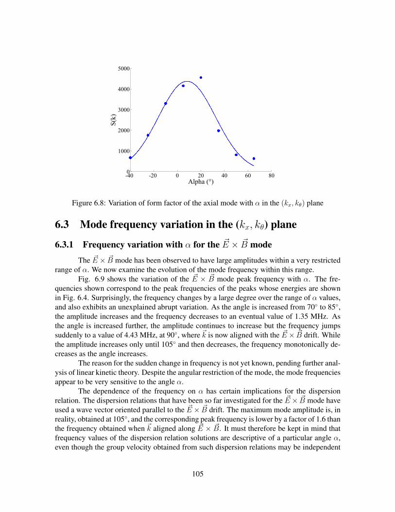
-40 -20 0 20 40 60 800
1000
2000
3000
4000
5000
S(k)
Alpha (°)
Figure 6.8: Variation of form factor of the axial mode with α in the (kx, kθ) plane
6.3 Mode frequency variation in the (kx, kθ) plane
6.3.1 Frequency variation with α for the ~E × ~B mode
The ~E × ~B mode has been observed to have large amplitudes within a very restrictedrange of α. We now examine the evolution of the mode frequency within this range.
Fig. 6.9 shows the variation of the ~E × ~B mode peak frequency with α. The fre-quencies shown correspond to the peak frequencies of the peaks whose energies are shownin Fig. 6.4. Surprisingly, the frequency changes by a large degree over the range of α values,and also exhibits an unexplained abrupt variation. As the angle is increased from 70 to 85,the amplitude increases and the frequency decreases to an eventual value of 1.35 MHz. Asthe angle is increased further, the amplitude continues to increase but the frequency jumpssuddenly to a value of 4.43 MHz, at 90, where ~k is now aligned with the ~E× ~B drift. Whilethe amplitude increases only until 105 and then decreases, the frequency monotonically de-creases as the angle increases.
The reason for the sudden change in frequency is not yet known, pending further anal-ysis of linear kinetic theory. Despite the angular restriction of the mode, the mode frequenciesappear to be very sensitive to the angle α.
The dependence of the frequency on α has certain implications for the dispersionrelation. The dispersion relations that have been so far investigated for the ~E× ~B mode haveused a wave vector oriented parallel to the ~E × ~B drift. The maximum mode amplitude is, inreality, obtained at 105, and the corresponding peak frequency is lower by a factor of 1.6 thanthe frequency obtained when ~k aligned along ~E × ~B. It must therefore be kept in mind thatfrequency values of the dispersion relation solutions are descriptive of a particular angle α,even though the group velocity obtained from such dispersion relations may be independent
105

60 70 80 90 100 110 120 1300
1
2
3
4
5x 10
6
Frequency (Hz)
Alpha (°)
Figure 6.9: Variation of the frequency of the positive frequency peak with α in the (kx, kθ)
plane, for the ~E × ~B mode
of α.
6.3.2 Frequency variation with α for the axial modeThe variation in frequency of the axial mode (positive frequency peak) with α is
shown in Fig. 6.10. The frequency variation observed is consistent with that expected if themode frequency were proportional to the projection of wavenumber along the axis x1. Thedata is fitted to a curve of the form f = Acos(θ + φ), and the fit parameters obtained are
A = 2.12× 10⁷ Hz, φ = 1.80 (6.8)
Interestingly, a fit of this form (in red in Fig. 6.10) fails to match the data, particularlyfor angles outside the range -40 < α < +40, where the frequencies are higher than wouldbe expected. It therefore appears that the idea of simple projection of the wave number (andvelocity) may not be accurate. Instead, a modified fit of the form f = Acos(nθ+φ) is applied(in blue in Fig. 6.10), for which the fit parameters are now
A = 2.06× 10⁷ Hz, n = 0.75, φ = 9.83 (6.9)
This modified fit is clearly superior. This seems consistent with the previous observa-tion that the dispersion relation for the axial mode is not a simple Doppler relation.
106

-40 -20 0 20 40 60 800.8
1
1.2
1.4
1.6
1.8
2
2.2x 10
7
Frequency (Hz)
Alpha (°)
Figure 6.10: Variation of frequency of the axial mode with α in the (kx, kθ) plane, with twofits applied: a simple cosine law (in red), and a modified cosine law (in blue)
6.4 Form factor variation in the (kx, kr) planeIn the configuration discussed in the previous section, in which the beams were
aligned along the z1 direction and parallel to the radial ~B field, the kr component was onthe order of its smallest possible value (the inverse channel dimension, or 250 rad/m). Theearly numerical simulations of the wave performed by Adam et. al. [2] were based solely onkθ and kx components (with kr = 0).
However, the influence of a wave vector component parallel to ~B cannot be neglected.For instance, as was mentioned after the first phase of experiments, the presence of a non-negligible kr could be sufficient to explain why the experimental dispersion relations, unlikethose derived from linear theory using kr = 0, are continuous. For this reason, and also tocomplete the study of directionality of the modes, it was decided to perform experiments withdifferent, known kr components.
New numerical solutions to the dispersion relation taking into account a non-negligiblekr component have been recently performed by A. Heron (Centre de Physique Theorique,Ecole Polytechnique) and these results will be discussed in the context of experimental datain a subsequent chapter.
6.4.1 Comparison of fluctuations perpendicular and parallel to ~B
The first experiment involving the addition of a kr component aims to compare themode amplitudes perpendicular to ~B and parallel to ~B. In the configuration shown in Fig.6.3, whatever the orientation of ~k in the (kx, kθ) plane, it is necessarily perpendicular to ~B.The sole configuration which permits an orientation of the wave vector purely parallel to ~B
107

(for a certain α) is the placement of the observation volume at the top or bottom thrusterchannel.
Fig. 6.11 shows the configuration adopted for one such experiment. To make thisexperiment possible, the thruster is raised by 47 mm inside the vacuum chamber, and theobservation volume lowered by 20 mm. The observation volume is finally situated a dis-tance h (67 mm) below the thruster axis. For measurements of the top thruster channel, themeasurement volume is situated 60 mm above the thruster axis.
Figure 6.11: Configuration for the measurement of ~k aligned along ~B; (a) shows a side viewfor the variation of α, (b) shows the orientation in which ~k may be aligned parallel to ~B,corresponding to α = 90
An angular exploration in α is carried out at the lower thruster channel to determinehow the mode amplitudes change as ~k becomes progressively more aligned with ~B. Thevalue of wave number is fixed at 5780 rad/m. The thruster exit plane is 17 mm from theobservation volume center, and the flow rate is 18 mg/s. The mean square amplitudes of themodes are presented in Fig. 6.12.
In Fig. 6.12, peaks pertaining to the axial mode, at α from -45 to 45, are present withrelatively high form factors. The form factor reaches a maximum of over 17000. Consistentwith earlier observations for this axial mode, this maximum in energy is not observed at 0,but a few degrees inclined with respect to the x1 axis. The Gaussian fit parameters obtainedfor this range of data are: A = 1.63×10⁴, µ = -17.3, and σ = 24.5. The significance of thenegative µ value will be discussed shortly.
In the range 100 < α < 150, signals corresponding to the axial mode are measured.This is possible because as the angle continues to increase, ~k becomes progressively moreoriented in the direction opposite to that of the the axial mode propagation. The ~E× ~B mode,
108

-50 0 50 100 1500
0.5
1
1.5
2x 10
4
S(k)
Alpha (°)
Figure 6.12: Variation in form factor of modes with α in the plane (kx, kr), for the observationvolume situated at the lower thruster channel (06h00). Points pertaining to the axial modepositive frequency peak are in blue; points pertaining to the axial mode negative frequencypeak are in red; points identified as the “cathode mode” are in black. A Gaussian curve(dotted line) is shown superposed on the axial mode positive frequency peak data
on the other hand, cannot be seen in this experimental configuration because ~k is alwayslocated in the (kx, kr) plane, and therefore perpendicular to ~E × ~B.
No signal is seen when α = 90, the angular value for which the wave vector is alignedparallel to ~B (and anti-parallel to kr).
A similar angular exploration is performed at the top thruster channel. The corre-sponding form factor trend is shown in Fig. 6.13.
As in the case of the lower channel, no signal is seen when α = 90, or at the symmet-ric position of α = 270. These experiments confirm that the neglect of density fluctuationsparallel to ~B in comparison with fluctuations perpendicular to ~B is indeed justified.
6.4.2 The “cathode” modeFig. 6.12 shows a number of points which correspond neither to the ~E × ~B mode
frequencies nor to the axial mode. These correspond to low-frequency, non-Gaussian peakswhich appear between 45 and 60. In the present work, this new mode has been named the“cathode mode” because it is seen during observations of the lower thruster channel only, thechannel position closest to where the cathode is located. The possible link of this mode to thecathode has been confirmed by an angular exploration in the (kx, kr) plane performed at thetop thruster channel. The observations of the axial mode positive and negative high frequencypeaks were repeated, however, the cathode mode was absent at the top thruster channel.
At α = 45, both cathode and axial modes can be identified. Fig. 6.14 shows the
109

-50 0 50 100 150 200 250 3000
0.5
1
1.5
2
2.5
3x 10
4
S(k)
Alpha (°)
Figure 6.13: Variation in form factor of modes with α in the plane (kx, kr), for the observationvolume situated at the upper thruster channel (12h00). Points pertaining to the axial modepositive frequency peak are in blue; points pertaining to the axial mode negative frequencypeak are in red. The cathode mode is absent. A Gaussian curve (dotted line) is shownsuperposed on the axial mode positive frequency peak data
frequency spectrum corresponding to this angle. The form factor of the cathode mode isnearly identical to that of the axial mode at this angle and appears to change little with α.
6.4.3 Axial mode width and mean angle in the (kx, kr) planeIt is interesting to consider how the axial mode mean angle and width in the (kx, kr)
plane change when the observation volume is situated at the top and bottom thruster channels.Apart from the observation of the cathode mode at the lower channel, are the 12h00 and06h00 positions on the azimuth otherwise symmetric? Fig. 6.15(a) and Fig. 6.15(b) show thevariation in form factor over α for the lower and upper thruster channels (positive frequencypeaks of the axial mode), for an angular exploration around α = 0.
The Gaussian fit parameters for the bottom thruster channel form factors are
A = 1.63× 10⁴, µ = −17.4, σ = 24.6 (6.10)
while for the top thruster channel the parameters are
A = 2.51× 10⁴, µ = 3.70, σ = 28.1 (6.11)
The angular widths are comparable to the on-axis case, and quite similar to eachother. However, it is interesting to observe here that the mean angle µ is very different at
110
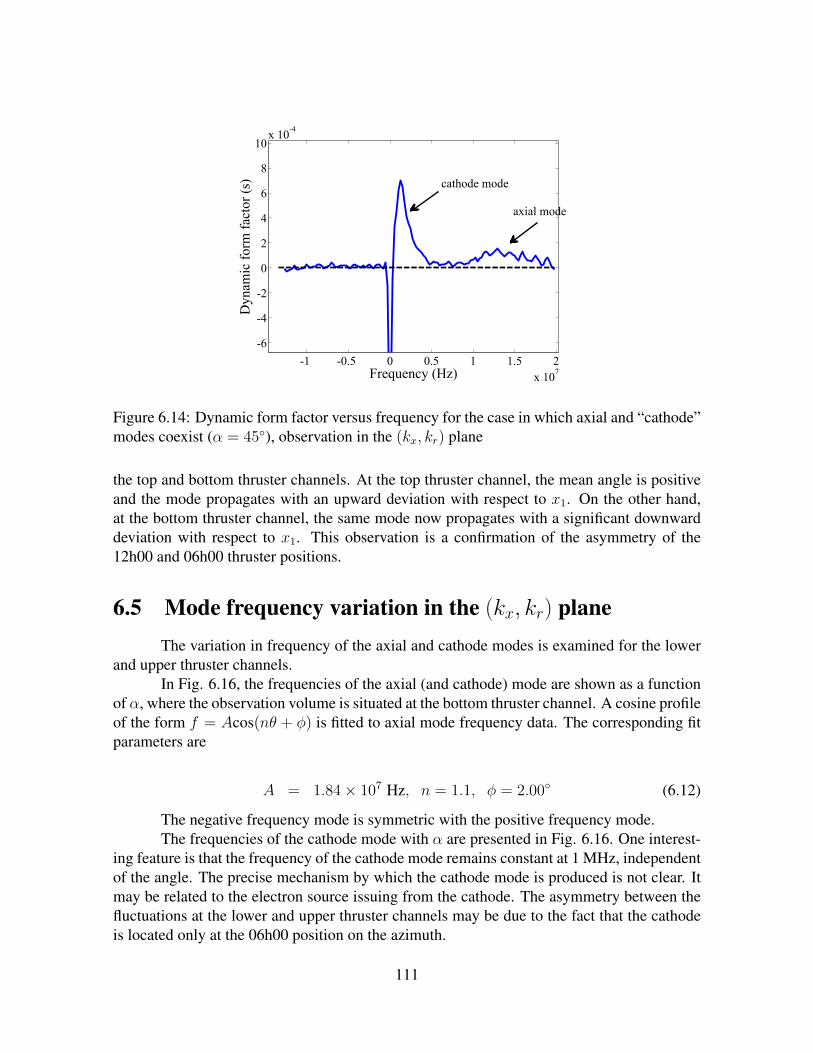
-1 -0.5 0 0.5 1 1.5 2
x 107
-6
-4
-2
0
2
4
6
8
10x 10
-4
Frequency (Hz)
Dynam
ic form
fac
tor (s) cathode mode
axial mode
Figure 6.14: Dynamic form factor versus frequency for the case in which axial and “cathode”modes coexist (α = 45), observation in the (kx, kr) plane
the top and bottom thruster channels. At the top thruster channel, the mean angle is positiveand the mode propagates with an upward deviation with respect to x1. On the other hand,at the bottom thruster channel, the same mode now propagates with a significant downwarddeviation with respect to x1. This observation is a confirmation of the asymmetry of the12h00 and 06h00 thruster positions.
6.5 Mode frequency variation in the (kx, kr) planeThe variation in frequency of the axial and cathode modes is examined for the lower
and upper thruster channels.In Fig. 6.16, the frequencies of the axial (and cathode) mode are shown as a function
of α, where the observation volume is situated at the bottom thruster channel. A cosine profileof the form f = Acos(nθ + φ) is fitted to axial mode frequency data. The corresponding fitparameters are
A = 1.84× 10⁷ Hz, n = 1.1, φ = 2.00 (6.12)
The negative frequency mode is symmetric with the positive frequency mode.The frequencies of the cathode mode with α are presented in Fig. 6.16. One interest-
ing feature is that the frequency of the cathode mode remains constant at 1 MHz, independentof the angle. The precise mechanism by which the cathode mode is produced is not clear. Itmay be related to the electron source issuing from the cathode. The asymmetry between thefluctuations at the lower and upper thruster channels may be due to the fact that the cathodeis located only at the 06h00 position on the azimuth.
111
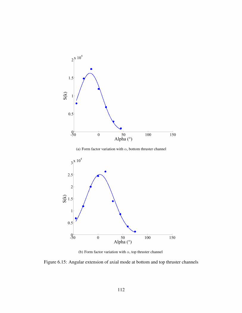
-50 0 50 100 1500
0.5
1
1.5
2x 10
4
S(k)
Alpha (°)
(a) Form factor variation with α, bottom thruster channel
-50 0 50 100 1500
0.5
1
1.5
2
2.5
3x 10
4
S(k)
Alpha (°)
(b) Form factor variation with α, top thruster channel
Figure 6.15: Angular extension of axial mode at bottom and top thruster channels
112
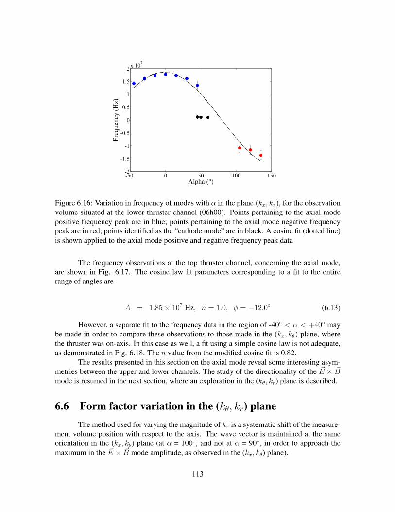
-50 0 50 100 150-2
-1.5
-1
-0.5
0
0.5
1
1.5
2x 10
7
Frequency (Hz)
Alpha (°)
Figure 6.16: Variation in frequency of modes with α in the plane (kx, kr), for the observationvolume situated at the lower thruster channel (06h00). Points pertaining to the axial modepositive frequency peak are in blue; points pertaining to the axial mode negative frequencypeak are in red; points identified as the “cathode mode” are in black. A cosine fit (dotted line)is shown applied to the axial mode positive and negative frequency peak data
The frequency observations at the top thruster channel, concerning the axial mode,are shown in Fig. 6.17. The cosine law fit parameters corresponding to a fit to the entirerange of angles are
A = 1.85× 10⁷ Hz, n = 1.0, φ = −12.0 (6.13)
However, a separate fit to the frequency data in the region of -40 < α < +40 maybe made in order to compare these observations to those made in the (kx, kθ) plane, wherethe thruster was on-axis. In this case as well, a fit using a simple cosine law is not adequate,as demonstrated in Fig. 6.18. The n value from the modified cosine fit is 0.82.
The results presented in this section on the axial mode reveal some interesting asym-metries between the upper and lower channels. The study of the directionality of the ~E × ~Bmode is resumed in the next section, where an exploration in the (kθ, kr) plane is described.
6.6 Form factor variation in the (kθ, kr) planeThe method used for varying the magnitude of kr is a systematic shift of the measure-
ment volume position with respect to the axis. The wave vector is maintained at the sameorientation in the (kx, kθ) plane (at α = 100, and not at α = 90, in order to approach themaximum in the ~E × ~B mode amplitude, as observed in the (kx, kθ) plane).
113
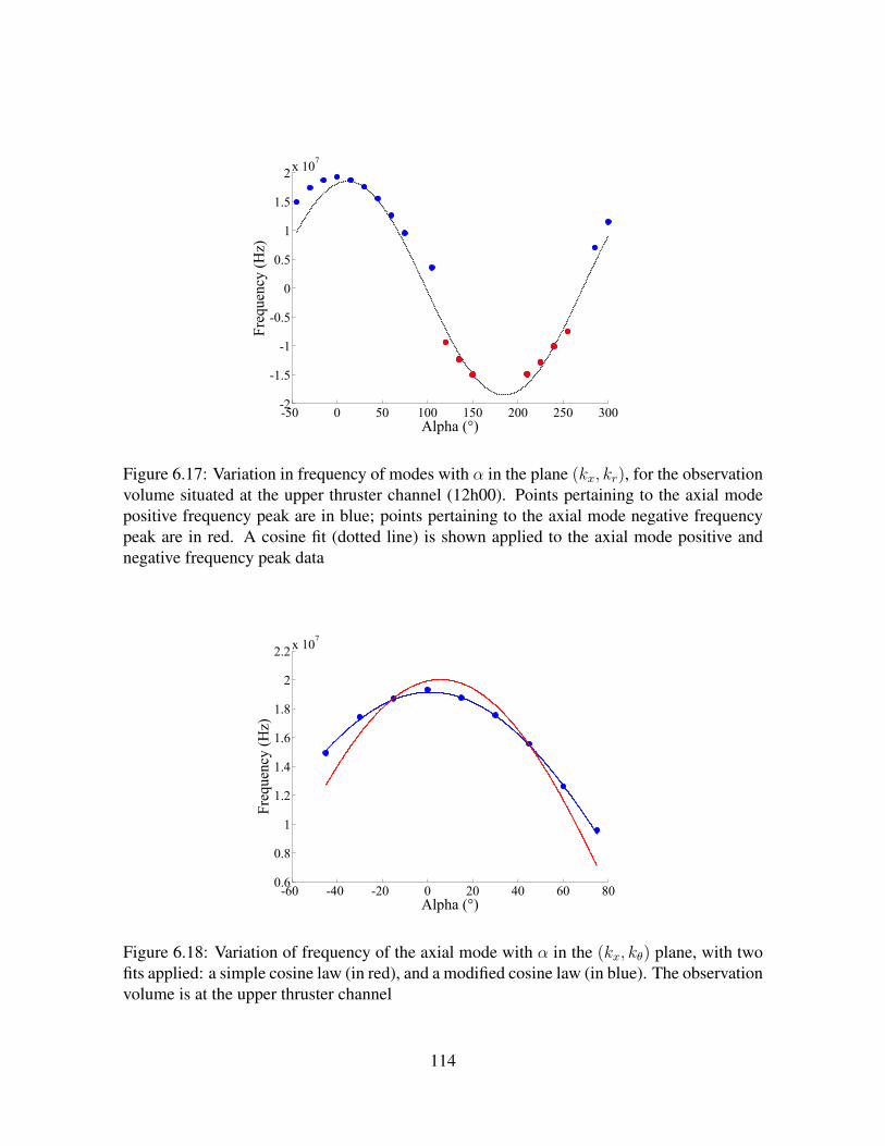
-50 0 50 100 150 200 250 300-2
-1.5
-1
-0.5
0
0.5
1
1.5
2x 10
7
Frequency (Hz)
Alpha (°)
Figure 6.17: Variation in frequency of modes with α in the plane (kx, kr), for the observationvolume situated at the upper thruster channel (12h00). Points pertaining to the axial modepositive frequency peak are in blue; points pertaining to the axial mode negative frequencypeak are in red. A cosine fit (dotted line) is shown applied to the axial mode positive andnegative frequency peak data
-60 -40 -20 0 20 40 60 800.6
0.8
1
1.2
1.4
1.6
1.8
2
2.2x 10
7
Frequency (Hz)
Alpha (°)
Figure 6.18: Variation of frequency of the axial mode with α in the (kx, kθ) plane, with twofits applied: a simple cosine law (in red), and a modified cosine law (in blue). The observationvolume is at the upper thruster channel
114
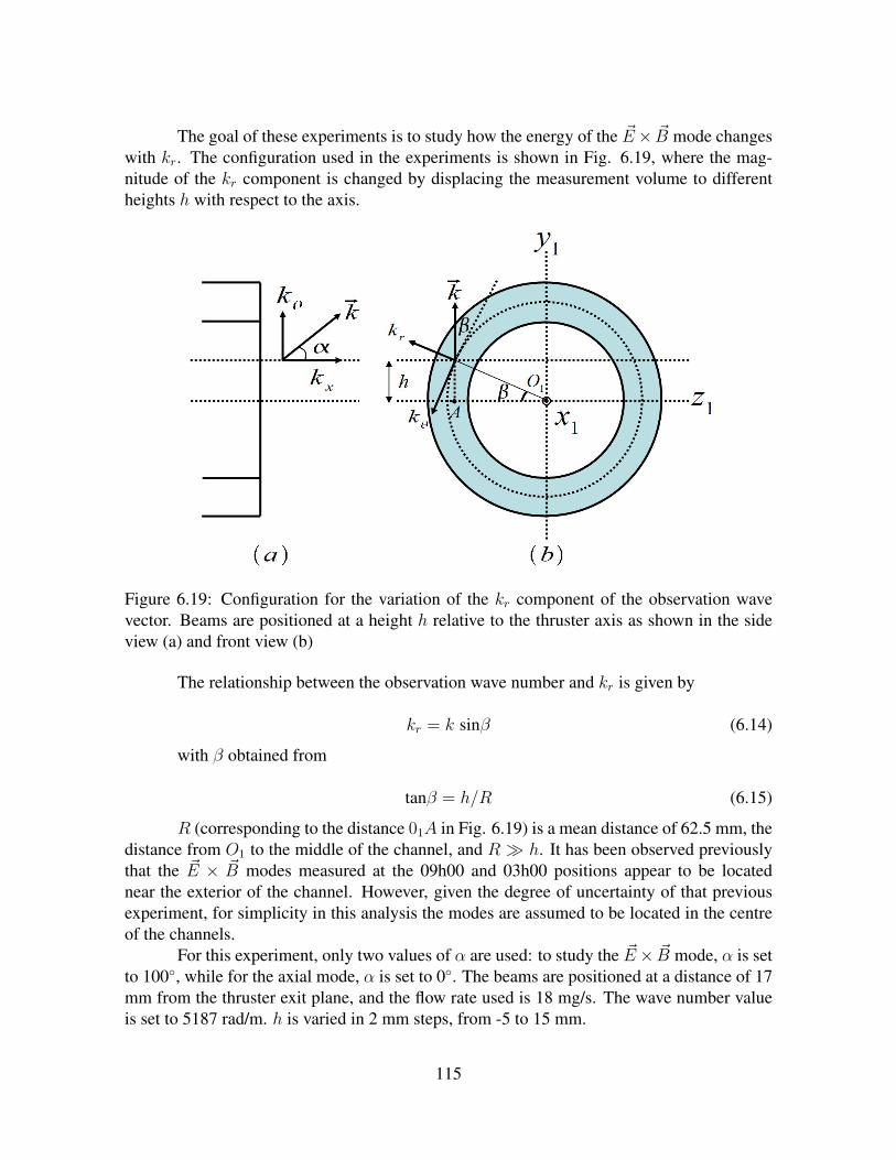
The goal of these experiments is to study how the energy of the ~E× ~B mode changeswith kr. The configuration used in the experiments is shown in Fig. 6.19, where the mag-nitude of the kr component is changed by displacing the measurement volume to differentheights h with respect to the axis.
Figure 6.19: Configuration for the variation of the kr component of the observation wavevector. Beams are positioned at a height h relative to the thruster axis as shown in the sideview (a) and front view (b)
The relationship between the observation wave number and kr is given by
kr = k sinβ (6.14)
with β obtained from
tanβ = h/R (6.15)
R (corresponding to the distance 01A in Fig. 6.19) is a mean distance of 62.5 mm, thedistance from O1 to the middle of the channel, and R h. It has been observed previouslythat the ~E × ~B modes measured at the 09h00 and 03h00 positions appear to be locatednear the exterior of the channel. However, given the degree of uncertainty of that previousexperiment, for simplicity in this analysis the modes are assumed to be located in the centreof the channels.
For this experiment, only two values of α are used: to study the ~E× ~B mode, α is setto 100, while for the axial mode, α is set to 0. The beams are positioned at a distance of 17mm from the thruster exit plane, and the flow rate used is 18 mg/s. The wave number valueis set to 5187 rad/m. h is varied in 2 mm steps, from -5 to 15 mm.
115

6.6.1 ~E × ~B mode directionality in the (kθ, kr) plane
The form factors of the ~E × ~B mode are determined for the different h values. Theform factors as a function of β are shown in Fig. 6.20.
-0.1 -0.05 0 0.05 0.1 0.15 0.2 0.250.4
0.6
0.8
1
1.2
1.4
1.6
1.8
2x 10
5
S(k)
β (rad)
Figure 6.20: Variation of form factor of the ~E × ~B mode with β (positive frequency peak)
The variation of form factor with β for this mode exhibits some surprising charac-teristics. The first observation of note is that the form factor of the mode is not maximumfor β = 0, the angle corresponding to the placement of the measurement volume along z1.Instead, the form factor reaches a maximum in energy (a very high level, 18.5×10⁴) at β =0.08 rad, or h = 5 mm. This is an indication that the mode is inclined in the plane y1O1z1, i.e.the ( ~E × ~B)− ~B plane. This inclination from the ~E × ~B drift direction is 4.58.
To determine the width of the form factor in β due to the device resolution, the for-mula for the longitudinal resolution, given by Eq. 1.14, is applied. In this case, the corre-sponding δβ is written
δβ =λ
2π√
2w(6.16)
The corresponding value of δβ is 4.11×10⁻⁴ rad. This value is sufficiently small tobe considered negligible in comparison with the peak width shown in Fig. 6.20.
The form factor distribution is also non-symmetric around its maximum. It is inter-esting to consider the distribution in the context of the negative frequency peak form factor,corresponding to observations in the other channel. The form factor distribution for this peakis shown in Fig. 6.21.
In Fig. 6.21, the observed form factor values are several orders of magnitude smallerthan those of the positive frequency peak; this is due to the fact that the particular value ofangle α used in this experiment (100) was chosen to obtain the maximum signal amplitude
116
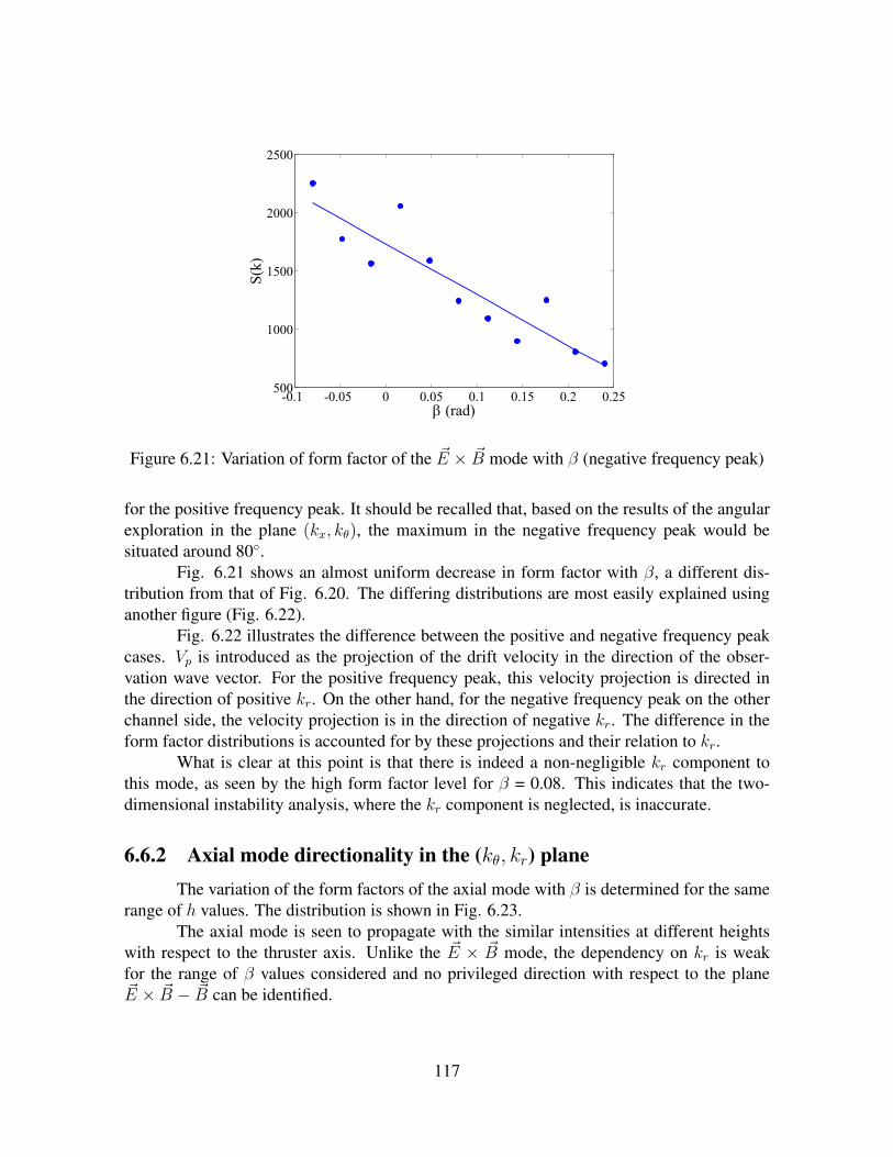
-0.1 -0.05 0 0.05 0.1 0.15 0.2 0.25500
1000
1500
2000
2500
S(k)
β (rad)
Figure 6.21: Variation of form factor of the ~E × ~B mode with β (negative frequency peak)
for the positive frequency peak. It should be recalled that, based on the results of the angularexploration in the plane (kx, kθ), the maximum in the negative frequency peak would besituated around 80.
Fig. 6.21 shows an almost uniform decrease in form factor with β, a different dis-tribution from that of Fig. 6.20. The differing distributions are most easily explained usinganother figure (Fig. 6.22).
Fig. 6.22 illustrates the difference between the positive and negative frequency peakcases. Vp is introduced as the projection of the drift velocity in the direction of the obser-vation wave vector. For the positive frequency peak, this velocity projection is directed inthe direction of positive kr. On the other hand, for the negative frequency peak on the otherchannel side, the velocity projection is in the direction of negative kr. The difference in theform factor distributions is accounted for by these projections and their relation to kr.
What is clear at this point is that there is indeed a non-negligible kr component tothis mode, as seen by the high form factor level for β = 0.08. This indicates that the two-dimensional instability analysis, where the kr component is neglected, is inaccurate.
6.6.2 Axial mode directionality in the (kθ, kr) planeThe variation of the form factors of the axial mode with β is determined for the same
range of h values. The distribution is shown in Fig. 6.23.The axial mode is seen to propagate with the similar intensities at different heights
with respect to the thruster axis. Unlike the ~E × ~B mode, the dependency on kr is weakfor the range of β values considered and no privileged direction with respect to the plane~E × ~B − ~B can be identified.
117

Figure 6.22: Configurations for kr (in blue), k (in black), Vd (in green) and Vp (in red) for theobservation of the positive and negative frequency peaks of the ~E × ~B mode
-0.1 -0.05 0 0.05 0.1 0.15 0.2 0.252000
3000
4000
5000
6000
7000
8000
9000
S(k)
β (rad)
Figure 6.23: Variation of form factor of the axial mode with β (positive frequency peak)
118
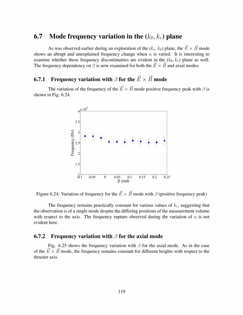
6.7 Mode frequency variation in the (kθ, kr) plane
As was observed earlier during an exploration of the (kx, kθ) plane, the ~E × ~B modeshows an abrupt and unexplained frequency change when α is varied. It is interesting toexamine whether these frequency discontinuities are evident in the (kθ, kr) plane as well.The frequency dependency on β is now examined for both the ~E × ~B and axial modes.
6.7.1 Frequency variation with β for the ~E × ~B mode
The variation of the frequency of the ~E × ~B mode positive frequency peak with β isshown in Fig. 6.24.
-0.1 -0.05 0 0.05 0.1 0.15 0.2 0.251
1.5
2
2.5
3
3.5
4x 10
6
Frequency (Hz)
β (rad)
Figure 6.24: Variation of frequency for the ~E × ~B mode with β (positive frequency peak)
The frequency remains practically constant for various values of kr, suggesting thatthe observation is of a single mode despite the differing positions of the measurement volumewith respect to the axis. The frequency rupture observed during the variation of α is notevident here.
6.7.2 Frequency variation with β for the axial modeFig. 6.25 shows the frequency variation with β for the axial mode. As in the case
of the ~E × ~B mode, the frequency remains constant for different heights with respect to thethruster axis.
119

-0.1 -0.05 0 0.05 0.1 0.15 0.2 0.251
1.5
2
2.5x 10
7
Frequency (Hz)
β (rad)
Figure 6.25: Variation of frequency for the axial mode with β (positive frequency peak)
6.8 Form factor of the ~E × ~B at three reference values of βwith varying α
To complete the study of directionality of the ~E × ~B mode, an exploration in α iscarried out for three different values of h. The earlier observations about the mode’s angularopening in the plane (kx, kθ) were made with the observation volume on the thruster axis,with h = 0. It is useful to determine whether these previous findings are dependent on themagnitude of the kr component present.
For this experiment, the three values of h used are -5, 5 and 15 mm (corresponding toβ of -0.08, 0.08 and 0.24). An α exploration is carried out between 75 and 130 to follow theevolution in form factor of the positive frequency peak of the mode.
The experimental conditions (18 mg/s flow rate, 17 mm separation between beamsand thruster exit plane) are maintained. The results of the exploration are shown in Fig. 6.26.
Standard Gaussian fits are applied to each set of points to obtain the amplitude, meanand peak widths. The results of these optimizations are given in Eq. 6.17. The values for β =-0.08, 0.08 and 0.24 have subscripts of 1, 2 and 3 respectively.
A1 = 1.69× 10⁵, µ1 = 105.1, σ1 = 6.28
A2 = 2.06× 10⁵, µ2 = 103.9, σ2 = 6.37
A3 = 0.877× 10⁵, µ3 = 104.0, σ3 = 6.19 (6.17)
It is interesting to note that, although the mode amplitude changes, the maximum inthe amplitude is attained at the same value of α for all three values of β. The values ofmean angle and standard deviation are very close for the three cases, and are very close to
120
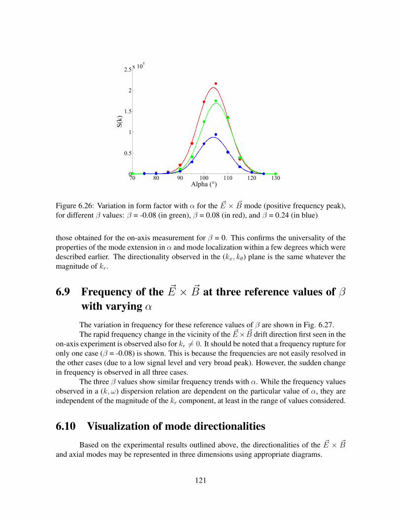
70 80 90 100 110 120 1300
0.5
1
1.5
2
2.5x 10
5
S(k)
Alpha (°)
Figure 6.26: Variation in form factor with α for the ~E × ~B mode (positive frequency peak),for different β values: β = -0.08 (in green), β = 0.08 (in red), and β = 0.24 (in blue)
those obtained for the on-axis measurement for β = 0. This confirms the universality of theproperties of the mode extension in α and mode localization within a few degrees which weredescribed earlier. The directionality observed in the (kx, kθ) plane is the same whatever themagnitude of kr.
6.9 Frequency of the ~E × ~B at three reference values of βwith varying αThe variation in frequency for these reference values of β are shown in Fig. 6.27.The rapid frequency change in the vicinity of the ~E× ~B drift direction first seen in the
on-axis experiment is observed also for kr 6= 0. It should be noted that a frequency rupture foronly one case (β = -0.08) is shown. This is because the frequencies are not easily resolved inthe other cases (due to a low signal level and very broad peak). However, the sudden changein frequency is observed in all three cases.
The three β values show similar frequency trends with α. While the frequency valuesobserved in a (k, ω) dispersion relation are dependent on the particular value of α, they areindependent of the magnitude of the kr component, at least in the range of values considered.
6.10 Visualization of mode directionalitiesBased on the experimental results outlined above, the directionalities of the ~E × ~B
and axial modes may be represented in three dimensions using appropriate diagrams.
121

60 70 80 90 100 110 120 1300
1
2
3
4
5
6x 10
6
Frequency (Hz)
Alpha (°)
Figure 6.27: Variation in frequency with α for the ~E × ~B mode (positive frequency peak),for different β values: β = -0.08 (in green), β = 0.08 (in red), and β = 0.24 (in blue)
6.10.1 ~E × ~B directionality
Fig. 6.28 shows the propagation orientation of the main ~E × ~B mode, identified bywave vector ~km. The angles α (90 + 10.6) and β (4.58) for the positive frequency peakshown in the figure are exaggerated for purposes of illustration.
A useful visualization is the form factor of the mode, based on its dependencies onα and β determined in this chapter. Fig. 6.29(a) provides such a visualization of the modeamplitude, with the contribution of the device resolution removed.
Fig. 6.29(b) shows a projection of the mode amplitude as a function of α and β whichcorresponds to the 3D view in Fig. 6.29(a). The thick horizontal line shows the absolutereference for β = 0 rad, the angle for which the observation volume is situated on-axis.
The thick vertical line on the projection indicates the reference angle which corre-sponds to the position of the axis Oy in the plane (kx, kθ). This angle, which would ideallybe 90, is corrected to take into account the indetermination of the positioning. The correctedreference angle used is 96.25, as mentioned earlier in Eq. 6.2.
6.10.2 Axial mode directionalityThe main direction of propagation of the axial mode is shown in Fig. 6.30, with an
angle α determined to be 8.22.
122
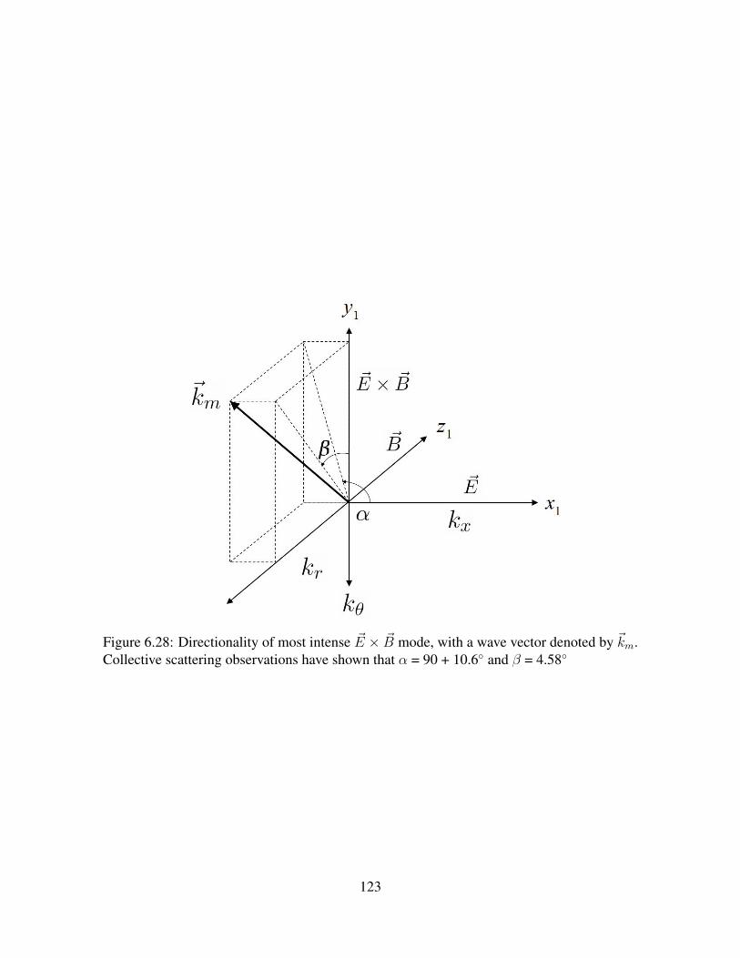
Figure 6.28: Directionality of most intense ~E × ~B mode, with a wave vector denoted by ~km.Collective scattering observations have shown that α = 90 + 10.6 and β = 4.58
123
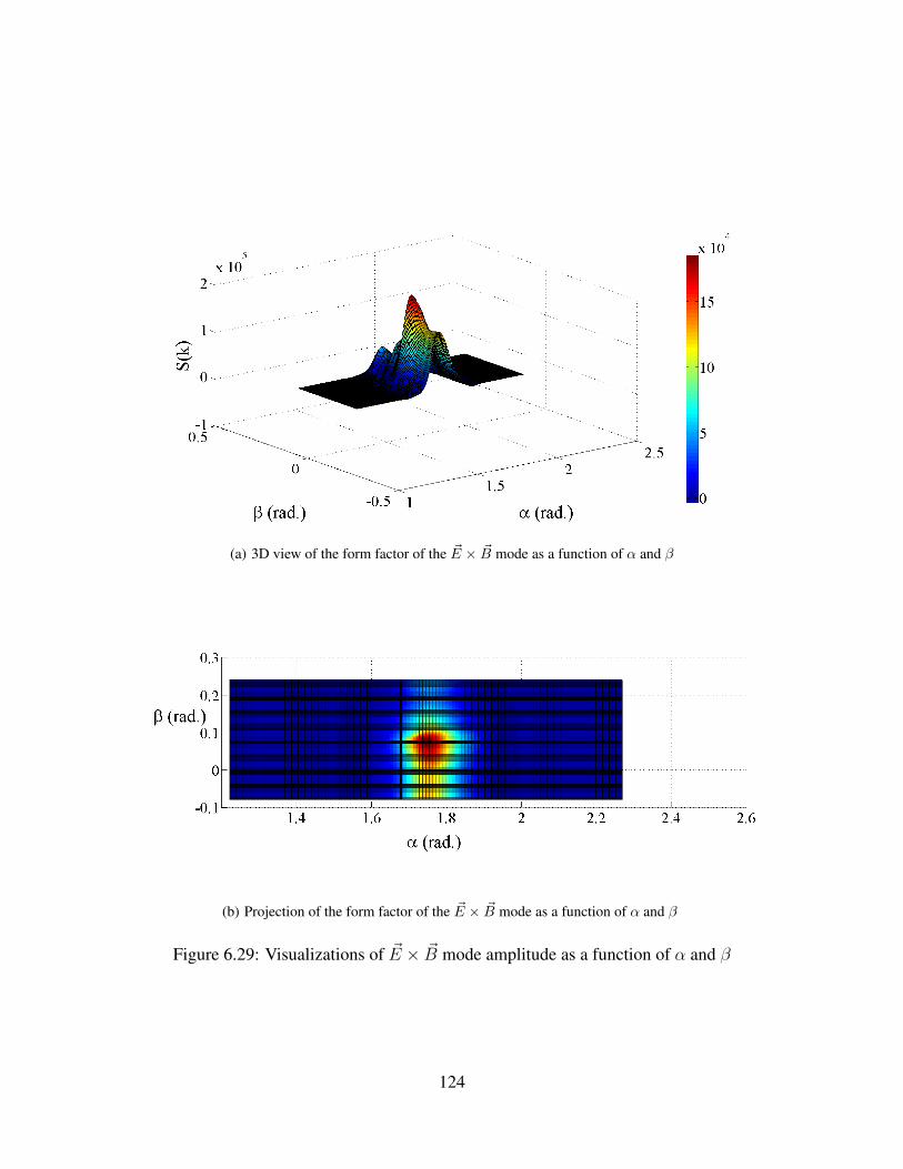
(a) 3D view of the form factor of the ~E × ~B mode as a function of α and β
(b) Projection of the form factor of the ~E × ~B mode as a function of α and β
Figure 6.29: Visualizations of ~E × ~B mode amplitude as a function of α and β
124

Figure 6.30: Directionality of most intense axial mode on-axis, with a wave vector denotedby ~km. Collective scattering observations have shown that α = 8.22 on-axis
6.11 Physical hypotheses concerning the directionality ofthe ~E × ~B mode
In Chapter 5, the radial non-uniformity in the electron cyclotron drift length was pro-posed to account for the apparent localization of the ~E × ~B mode near the outer channelwall. This non-uniformity may be at the origin of the inclination observed with respect to the~E × ~B drift observed in this chapter, and in particular, the presence of a non-negligible krcomponent.
However, this is only a hypothesis. To explore its validity, an extension must bemade of the linear kinetic theory of the instability to a non-uniform plasma. The variation ofthe form factor with kr, with the angle of maximum emission β discovered experimentally,should also be compared with the linear growth rate obtained from linear kinetic theory andthe dependence of this growth rate on kr.
Another hypothesis, concerning the inclination of the ~E× ~B mode towards the thrusterface in the (kx, kθ) plane, may be proposed. It is quite intriguing that the angle α made bythe principal axial mode with the x1, 8, is on the same order as the angle made by the main~E × ~B mode with the ~E × ~B drift direction, 10.6. The two modes have little in commonbeyond this particular characteristic.
Fig. 6.31 illustrates the situation described above, with ~ka denoting the main direc-tion of propagation of the axial mode in the plane (kx, kθ). ~ke shows the main direction ofpropagation of the ~E × ~B mode.
The axial mode has been identified as resulting from the convection of electrons bythe exiting ions, and it provides an indirect means by which the effect of the ion propagationon the ~E × ~B mode may be characterized. The ions have a damping effect on the electronmotion, and the inclination of the ~E × ~B mode could very easily result from the fact thatthis is a required angle for the ~E × ~B mode to avoid damping by the ion velocity. With this
125

Figure 6.31: Near-orthogonal propagation directions of the main ~E × ~B and axial modes inthe (kx, kθ) plane. ~ka represents the axial wave vector, ~ke the wave vector of the ~E× ~B mode
inclination, the most intense axial and ~E × ~B modes are separated by about 90. Away fromthis angle, the ~E× ~B is quickly subject to damping and its range is therefore restricted, whichalso accounts for its narrow region of propagation (3.0) in this plane.
6.12 Redetermination of the density fluctuation rate
With these more precise characterizations of the ~E × ~B mode, and the certitude thatthe signal registered is not subject to losses due to heterodyning, the density fluctuation ratemay now be more accurately estimated.
The form factor dependency on wavenumber has been shown to be an exponential:S(k) = S0e
−bk. In an earlier experiment during this campaign in which the maximum valueof S(k) was observed, the parameters of the exponential were
S0 = 4.64× 10⁶, b = 6.78× 10⁻⁴ m (6.18)
A further adjustment to S0 is obtained from the observations made of the variation ofS(k) with β. As has been shown, the maximum amplitude of the ~E × ~B mode is obtainednot for β = 0 (with the beams on-axis), but with β = 0.08 rad (with the beams positioned 5mm above the thruster axis). The value of S0 in Eq. 6.18 was obtained in an experiment forwhich β = 0. To estimate the true maximum value which would be expected at β = 0.08,S0 is scaled using the relative mode amplitudes in Fig. 6.20. The scaling factor is 1.4.Consequently, the adjusted S0 value is 6.5×10⁶.
The main idea here is that the optical bench is capable of measuring (and does) asignal level which is representative of the true energy level of the fluctuation. The densityfluctuation rate must therefore be determined using the maximum signal level obtained ex-perimentally.
126

From the α exploration for this mode, it was determined that the angular opening ofthe mode in the (kx, kθ) plane is 3.0, or 0.05 rad. This value will be identified here as σα;the value of the location of the most intense mode (90 + 10.6) will be identified here as µα.The β value is 0.08 rad and the peak width ∆β is estimated at about 0.15 rad.
One key assumption in the first phase of experiments was that the ~k component par-allel to ~B was small, on the order of the inverse channel width, and constant; this has beenproven in this chapter to be false. The re-evaluated mean square density fluctuation expres-sion is written
⟨n2⟩≈ S0n0
(2π)3
∫0
∞e−kbdk
∫ke− (α−µα)2
2σα2 dαk∆β (6.19)
This integral reduces to ⟨n2⟩≈ ασ∆β
23/2π5/2b3n0L (6.20)
in which L is the total channel length which coincides with the scattering volume, i.e.for a channel width of 25 mm, L is 50 mm because the measurement volume always traversesthe entire thruster diameter.
The mean square density fluctuation is⟨n2⟩≈ 0.76× 1031 m−6 (6.21)
The corresponding r.m.s density fluctuation value is 2.76×10¹⁵ m−3. Once again, thedensity fluctuation rate is obtained using a mean density of 1018 m−3,√
〈n2〉n0
= 2.8× 10⁻³ (6.22)
This density fluctuation rate is a factor 7 larger than that calculated from the experi-ments and assumptions from Part I, but remains very low, only 0.3%.
The results described in this chapter provide new information on the directionality ofboth the axial and ~E × ~B modes. The directionality studies have revealed the propagation ofthe ~E × ~B mode in three dimensions, contrary to the original simplified 2D view proposedin Part I, and that adopted in linear kinetic theory. The newly-evaluated density fluctuationlevel is low and now must be interpreted in terms of the possible transport mechanism.
127

Chapter 7
Detailed comparisons between linearkinetic theory and experiment
Contents7.1 Introduction . . . . . . . . . . . . . . . . . . . . . . . . . . . . . . . . . 128
7.2 The three dimensional dispersion relation . . . . . . . . . . . . . . . . . 129
7.3 The influence of kz on the dispersion relation . . . . . . . . . . . . . . . 130
7.3.1 The dispersion relation for vthe/Vd = 1.8 . . . . . . . . . . . . . . 130
7.3.2 The dispersion relation for vthe/Vd = 2.5 . . . . . . . . . . . . . . 131
7.3.3 Effect on dispersion relation of increasing kz . . . . . . . . . . . . 135
7.4 Variation of frequency with α . . . . . . . . . . . . . . . . . . . . . . . . 137
7.4.1 Frequency variation with α for k = 6400 rad/m . . . . . . . . . . . 137
7.4.2 Frequency variation with α for k = 8800 rad/m . . . . . . . . . . . 139
7.5 Variation of kz component . . . . . . . . . . . . . . . . . . . . . . . . . 139
7.5.1 Variation of kz for k = 6000 rad/m . . . . . . . . . . . . . . . . . . 139
7.5.2 Variation of kz for k = 8000 rad/m . . . . . . . . . . . . . . . . . . 141
7.6 Resonance conditions and stochasticity . . . . . . . . . . . . . . . . . . 141
7.7 Applications to the Hall thruster . . . . . . . . . . . . . . . . . . . . . . 143
7.1 Introduction
IN Chapter 3, a first comparison of the experimental results to the 1D (ky) and 2D (ky,kx) theoretical dispersion relations was made. The predicted theoretical frequency and
128
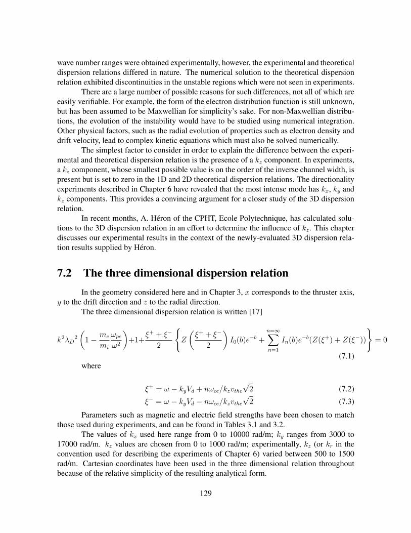
wave number ranges were obtained experimentally, however, the experimental and theoreticaldispersion relations differed in nature. The numerical solution to the theoretical dispersionrelation exhibited discontinuities in the unstable regions which were not seen in experiments.
There are a large number of possible reasons for such differences, not all of which areeasily verifiable. For example, the form of the electron distribution function is still unknown,but has been assumed to be Maxwellian for simplicity’s sake. For non-Maxwellian distribu-tions, the evolution of the instability would have to be studied using numerical integration.Other physical factors, such as the radial evolution of properties such as electron density anddrift velocity, lead to complex kinetic equations which must also be solved numerically.
The simplest factor to consider in order to explain the difference between the experi-mental and theoretical dispersion relation is the presence of a kz component. In experiments,a kz component, whose smallest possible value is on the order of the inverse channel width, ispresent but is set to zero in the 1D and 2D theoretical dispersion relations. The directionalityexperiments described in Chapter 6 have revealed that the most intense mode has kx, ky andkz components. This provides a convincing argument for a closer study of the 3D dispersionrelation.
In recent months, A. Heron of the CPHT, Ecole Polytechnique, has calculated solu-tions to the 3D dispersion relation in an effort to determine the influence of kz. This chapterdiscusses our experimental results in the context of the newly-evaluated 3D dispersion rela-tion results supplied by Heron.
7.2 The three dimensional dispersion relationIn the geometry considered here and in Chapter 3, x corresponds to the thruster axis,
y to the drift direction and z to the radial direction.The three dimensional dispersion relation is written [17]
k2λD2
(1− me
mi
ωpeω2
)+1+
ξ+ + ξ−
2
Z
(ξ+ + ξ−
2
)I0(b)e−b +
n=∞∑n=1
In(b)e−b(Z(ξ+) + Z(ξ−))
= 0
(7.1)where
ξ+ = ω − kyVd + nωce/kzvthe√
2 (7.2)
ξ− = ω − kyVd − nωce/kzvthe√
2 (7.3)
Parameters such as magnetic and electric field strengths have been chosen to matchthose used during experiments, and can be found in Tables 3.1 and 3.2.
The values of kx used here range from 0 to 10000 rad/m; ky ranges from 3000 to17000 rad/m. kz values are chosen from 0 to 1000 rad/m; experimentally, kz (or kr in theconvention used for describing the experiments of Chapter 6) varied between 500 to 1500rad/m. Cartesian coordinates have been used in the three dimensional relation throughoutbecause of the relative simplicity of the resulting analytical form.
129

7.3 The influence of kz on the dispersion relationIn Chapter 3, the unstable regions were limited to comb-like lobes. The case is dra-
matically different when a kz component is included: from kz = 230 rad/m onwards, theunstable modes become continuous and the instability is present over the entire range of kyvalues. This section describes the effect of the presence of a non-negligible kz on the disper-sion relation. Here, kz is set to 470 rad/m.
This value of kz is chosen as representative of the lower limit of kz during the explo-rations in the (kθ, kr) plane. During these experiments, for an observation wave number ofabout 6000 rad/m, kz was varied from 480 - 1440 rad/m.
Two cases are now considered: (i) a low electron temperature (vthe/Vd = 1.8), and (ii)an electron temperature corresponding to that determined from the experimental dispersionrelation (16 eV), i.e. vthe/Vd = 2.5. The value of 16 eV was determined by consideringthe wave (reasonably) as an ion acoustic wave, however, no direct measure of the electrontemperature for the wave is available.
The frequency and growth rates will be given in Hz to facilitate comparison to theexperimental results.
7.3.1 The dispersion relation for vthe/Vd = 1.8The dispersion relation is numerically solved to give the frequency of the instability
ωr and its growth rate γ as defined in Chapter 3 for vthe/Vd = 1.8. Fig. 7.1 shows dispersionrelation frequency as a function of kx and ky.
Figure 7.1: Frequency (Hz) as a function of ky and kx, for kz = 470 rad/m and vthe/Vd = 1.8
The discontinuity visible in the 2D case has disappeared. The unstable regions havebroadened significantly and some form of instability is visible at all values of ky. This broad-ening in the unstable region is accompanied by a reduction in the growth rate of the instability,
130
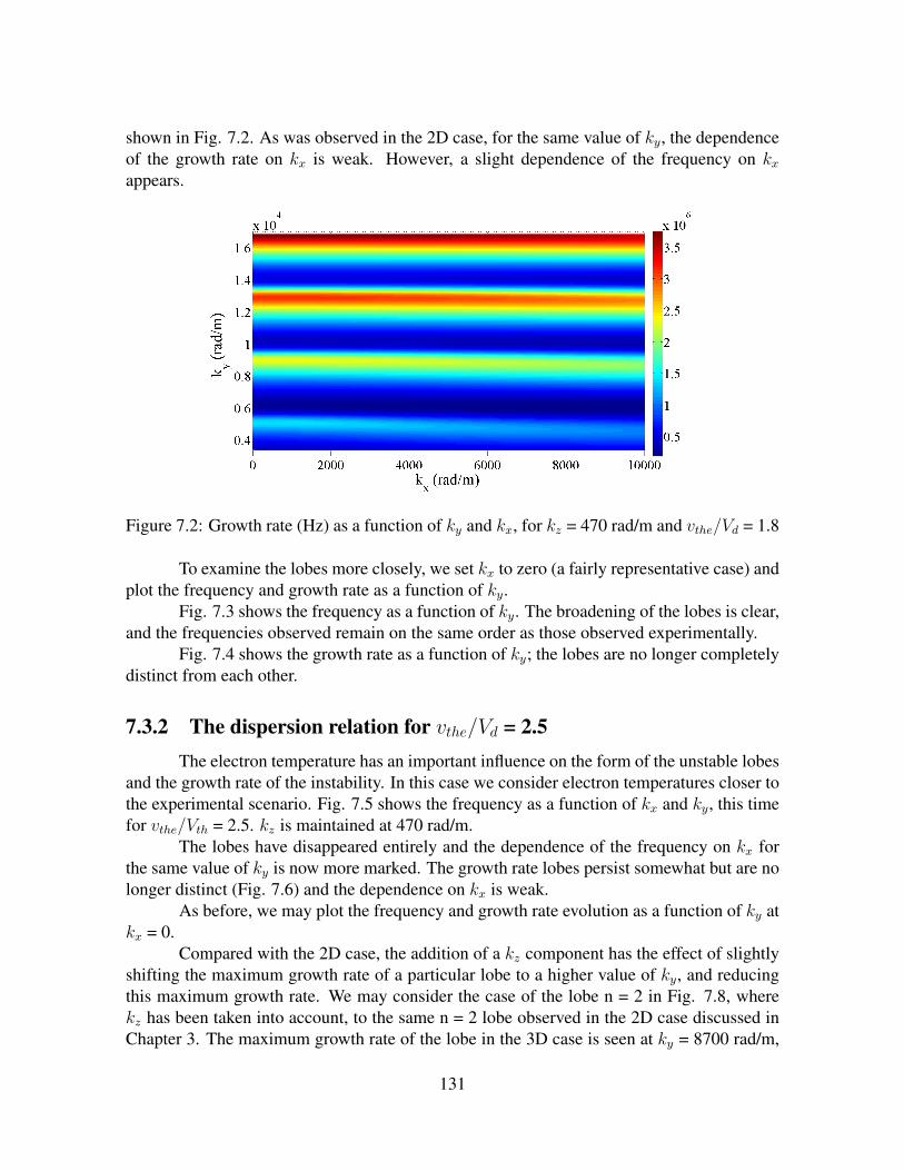
shown in Fig. 7.2. As was observed in the 2D case, for the same value of ky, the dependenceof the growth rate on kx is weak. However, a slight dependence of the frequency on kxappears.
Figure 7.2: Growth rate (Hz) as a function of ky and kx, for kz = 470 rad/m and vthe/Vd = 1.8
To examine the lobes more closely, we set kx to zero (a fairly representative case) andplot the frequency and growth rate as a function of ky.
Fig. 7.3 shows the frequency as a function of ky. The broadening of the lobes is clear,and the frequencies observed remain on the same order as those observed experimentally.
Fig. 7.4 shows the growth rate as a function of ky; the lobes are no longer completelydistinct from each other.
7.3.2 The dispersion relation for vthe/Vd = 2.5The electron temperature has an important influence on the form of the unstable lobes
and the growth rate of the instability. In this case we consider electron temperatures closer tothe experimental scenario. Fig. 7.5 shows the frequency as a function of kx and ky, this timefor vthe/Vth = 2.5. kz is maintained at 470 rad/m.
The lobes have disappeared entirely and the dependence of the frequency on kx forthe same value of ky is now more marked. The growth rate lobes persist somewhat but are nolonger distinct (Fig. 7.6) and the dependence on kx is weak.
As before, we may plot the frequency and growth rate evolution as a function of ky atkx = 0.
Compared with the 2D case, the addition of a kz component has the effect of slightlyshifting the maximum growth rate of a particular lobe to a higher value of ky, and reducingthis maximum growth rate. We may consider the case of the lobe n = 2 in Fig. 7.8, wherekz has been taken into account, to the same n = 2 lobe observed in the 2D case discussed inChapter 3. The maximum growth rate of the lobe in the 3D case is seen at ky = 8700 rad/m,
131

0.4 0.6 0.8 1 1.2 1.4 1.6 1.8 2
x 104
1
2
3
4
5
6
7x 10
6
ky (rad/m)
Frequency (Hz)
Figure 7.3: Frequency as a function of ky, for kx = 0, kz = 470 rad/m and vthe/Vd = 1.8
0.4 0.6 0.8 1 1.2 1.4 1.6 1.8 2
x 104
0
0.5
1
1.5
2
2.5
3
3.5
4x 10
6
ky (rad/m)
Growth rate (Hz)
Figure 7.4: Growth rate as a function of ky, for kx = 0, kz = 470 rad/m and vthe/Vd = 1.8
132

Figure 7.5: Frequency as a function of ky and kx, for kz = 470 rad/m and vthe/Vd = 2.5
Figure 7.6: Growth rate as a function of ky and kx, for kz = 470 rad/m and vthe/Vd = 2.5
133
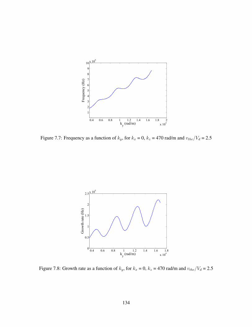
0.4 0.6 0.8 1 1.2 1.4 1.6 1.8 2
x 104
1
2
3
4
5
6
7
8
9
10x 10
6
ky (rad/m)
Frequency (Hz)
Figure 7.7: Frequency as a function of ky, for kx = 0, kz = 470 rad/m and vthe/Vd = 2.5
0.4 0.6 0.8 1 1.2 1.4 1.6 1.8
x 104
0
0.5
1
1.5
2
2.5x 10
6
ky (rad/m)
Growth rate (Hz)
Figure 7.8: Growth rate as a function of ky, for kx = 0, kz = 470 rad/m and vthe/Vd = 2.5
134

while it is seen at ky = 8500 rad/m in the 2D case. The maximum growth rate for this lobe inthe 3D case is 1.5×10⁶ Hz in the 3D case, and 9.1×10⁶ Hz in the 2D case.
7.3.3 Effect on dispersion relation of increasing kzThe effect of increasing kz from 470 to 1000 rad/m is studied in this section. 1000
rad/m is in the upper range of kz values used experimentally.The frequency and growth rates as a function of ky and kx for kz = 1000 rad/m are
shown in Fig. 7.9 and Fig. 7.10.
Figure 7.9: Frequency as a function of ky and kx, for kz = 1000 rad/m and vthe/Vd = 2.5
Figure 7.10: Growth rate as a function of ky and kx, for kz = 1000 rad/m and vthe/Vd = 2.5
135
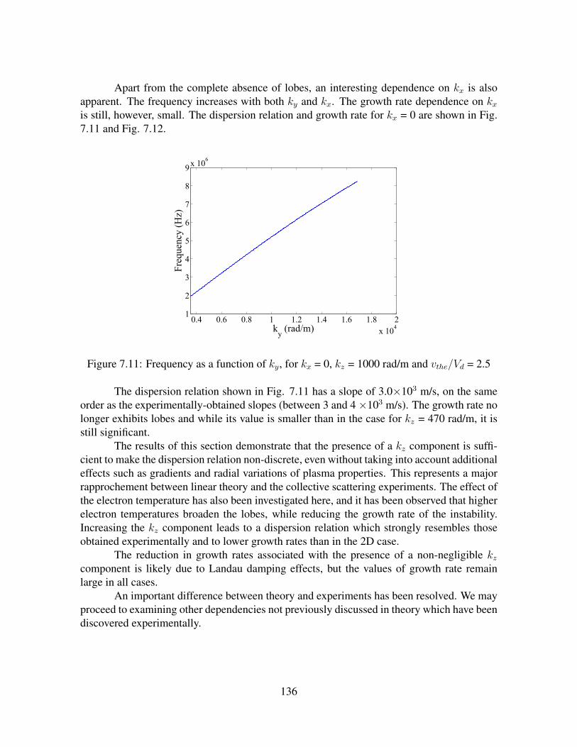
Apart from the complete absence of lobes, an interesting dependence on kx is alsoapparent. The frequency increases with both ky and kx. The growth rate dependence on kxis still, however, small. The dispersion relation and growth rate for kx = 0 are shown in Fig.7.11 and Fig. 7.12.
0.4 0.6 0.8 1 1.2 1.4 1.6 1.8 2
x 104
1
2
3
4
5
6
7
8
9x 10
6
ky (rad/m)
Frequency (Hz)
Figure 7.11: Frequency as a function of ky, for kx = 0, kz = 1000 rad/m and vthe/Vd = 2.5
The dispersion relation shown in Fig. 7.11 has a slope of 3.0×10³ m/s, on the sameorder as the experimentally-obtained slopes (between 3 and 4 ×10³ m/s). The growth rate nolonger exhibits lobes and while its value is smaller than in the case for kz = 470 rad/m, it isstill significant.
The results of this section demonstrate that the presence of a kz component is suffi-cient to make the dispersion relation non-discrete, even without taking into account additionaleffects such as gradients and radial variations of plasma properties. This represents a majorrapprochement between linear theory and the collective scattering experiments. The effect ofthe electron temperature has also been investigated here, and it has been observed that higherelectron temperatures broaden the lobes, while reducing the growth rate of the instability.Increasing the kz component leads to a dispersion relation which strongly resembles thoseobtained experimentally and to lower growth rates than in the 2D case.
The reduction in growth rates associated with the presence of a non-negligible kzcomponent is likely due to Landau damping effects, but the values of growth rate remainlarge in all cases.
An important difference between theory and experiments has been resolved. We mayproceed to examining other dependencies not previously discussed in theory which have beendiscovered experimentally.
136
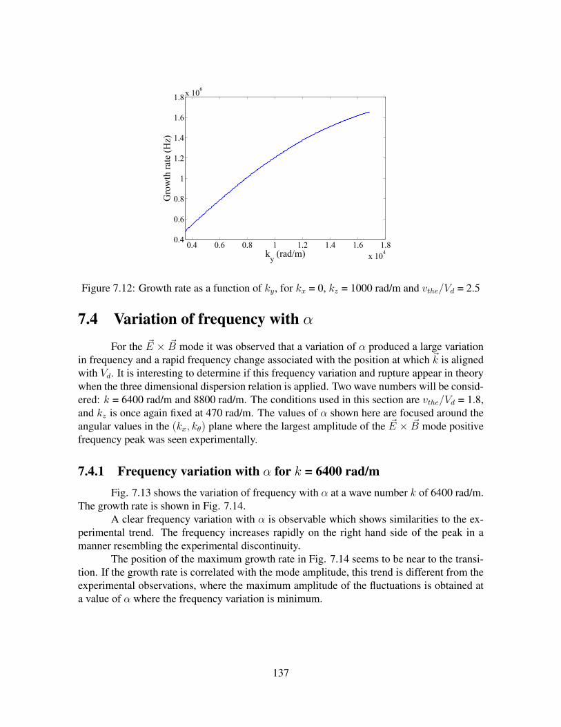
0.4 0.6 0.8 1 1.2 1.4 1.6 1.8
x 104
0.4
0.6
0.8
1
1.2
1.4
1.6
1.8x 10
6
ky (rad/m)
Growth rate (Hz)
Figure 7.12: Growth rate as a function of ky, for kx = 0, kz = 1000 rad/m and vthe/Vd = 2.5
7.4 Variation of frequency with α
For the ~E × ~B mode it was observed that a variation of α produced a large variationin frequency and a rapid frequency change associated with the position at which ~k is alignedwith Vd. It is interesting to determine if this frequency variation and rupture appear in theorywhen the three dimensional dispersion relation is applied. Two wave numbers will be consid-ered: k = 6400 rad/m and 8800 rad/m. The conditions used in this section are vthe/Vd = 1.8,and kz is once again fixed at 470 rad/m. The values of α shown here are focused around theangular values in the (kx, kθ) plane where the largest amplitude of the ~E × ~B mode positivefrequency peak was seen experimentally.
7.4.1 Frequency variation with α for k = 6400 rad/mFig. 7.13 shows the variation of frequency with α at a wave number k of 6400 rad/m.
The growth rate is shown in Fig. 7.14.A clear frequency variation with α is observable which shows similarities to the ex-
perimental trend. The frequency increases rapidly on the right hand side of the peak in amanner resembling the experimental discontinuity.
The position of the maximum growth rate in Fig. 7.14 seems to be near to the transi-tion. If the growth rate is correlated with the mode amplitude, this trend is different from theexperimental observations, where the maximum amplitude of the fluctuations is obtained ata value of α where the frequency variation is minimum.
137

90 100 110 120 130 140 1502.2
2.4
2.6
2.8
3
3.2
3.4x 10
6
Alpha (°)
Frequency (Hz)
Figure 7.13: Frequency as a function of α, for k = 6400 rad/m
90 100 110 120 130 140 1502
4
6
8
10
12
14x 10
5
Alpha (°)
Growth rate (Hz)
Figure 7.14: Growth rate as a function of α, for k = 6400 rad/m
138
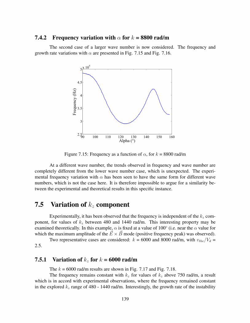
7.4.2 Frequency variation with α for k = 8800 rad/mThe second case of a larger wave number is now considered. The frequency and
growth rate variations with α are presented in Fig. 7.15 and Fig. 7.16.
90 100 110 120 130 140 150 1602.5
3
3.5
4
4.5
5x 10
6
Alpha (°)
Frequency (Hz)
Figure 7.15: Frequency as a function of α, for k = 8800 rad/m
At a different wave number, the trends observed in frequency and wave number arecompletely different from the lower wave number case, which is unexpected. The experi-mental frequency variation with α has been seen to have the same form for different wavenumbers, which is not the case here. It is therefore impossible to argue for a similarity be-tween the experimental and theoretical results in this specific instance.
7.5 Variation of kz componentExperimentally, it has been observed that the frequency is independent of the kz com-
ponent, for values of kz between 480 and 1440 rad/m. This interesting property may beexamined theoretically. In this example, α is fixed at a value of 100 (i.e. near the α value forwhich the maximum amplitude of the ~E × ~B mode (positive frequency peak) was observed).
Two representative cases are considered: k = 6000 and 8000 rad/m, with vthe/Vd =2.5.
7.5.1 Variation of kz for k = 6000 rad/mThe k = 6000 rad/m results are shown in Fig. 7.17 and Fig. 7.18.The frequency remains constant with kz for values of kz above 750 rad/m, a result
which is in accord with experimental observations, where the frequency remained constantin the explored kz range of 480 - 1440 rad/m. Interestingly, the growth rate of the instability
139
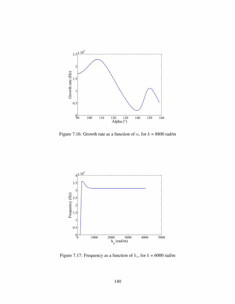
90 100 110 120 130 140 150 1600
0.5
1
1.5
2
2.5x 10
6
Alpha (°)
Growth rate (Hz)
Figure 7.16: Growth rate as a function of α, for k = 8800 rad/m
0 1000 2000 3000 4000 50000
0.5
1
1.5
2
2.5
3
3.5
4x 10
6
kz (rad/m)
Frequency (Hz)
Figure 7.17: Frequency as a function of kz, for k = 6000 rad/m
140

0 1000 2000 3000 4000 50000
1
2
3
4
5
6
7
8x 10
5
kz (rad/m)
Growth rate (Hz)
Figure 7.18: Growth rate as a function of kz, for k = 6000 rad/m
is maximum when kz 6= 0. In addition, the growth rate varies less with kz than it does withα. In experiments, the mode amplitude was seen to vary more markedly with α than with theangle β, and there may be a connection between this observation and the growth rate.
7.5.2 Variation of kz for k = 8000 rad/mWhen the wave number is changed, a similar trend in frequency is observed which
agrees with the experimental observations.The trend in growth rate is different from that observed in the k = 6000 rad/m case,
and the reason for this is not clear. For a value of α different from 100, for instance, 90,where ~k is now parallel to the ~E × ~B drift direction, very similar results are obtained.
The numerical results so far discussed demonstrate some interesting agreements be-tween the experimental and theoretical dispersion relations when kz is taken into account.Certain other features such as the frequency dependency on kz are the same in the experi-mental and theoretical cases. The influence of the electron density has also been studied (butnot described in this work) and it has been seen to have a negligible effect on the instability.
It is now worth re-evaluating electron transport in the context of the experimental re-sults. The question at stake here is whether electron transport across field lines can occurunder the actual experimental conditions due to the presence of the wave whose characteris-tics have been measured experimentally.
7.6 Resonance conditions and stochasticityThe experiments described in this work have revealed the presence of an azimuthal
wave with characteristics predicted by Adam et. al [2]. The link between this wave and axial
141

0 1000 2000 3000 4000 5000 6000 70000
1
2
3
4
5x 10
6
kz (rad/m)
Frequency (Hz)
Figure 7.19: Frequency as a function of kz, for k = 8000 rad/m
0 1000 2000 3000 4000 5000 6000 70000
5
10
15x 10
5
kz (rad/m)
Growth rate (Hz)
Figure 7.20: Growth rate as a function of kz, for k = 8000 rad/m
142

electron transport may be provided by a particle-heating mechanism first described in detailby C. F. F. Karney [37] for a crossed electric and magnetic field configuration.
C. F. F. Karney proposed that lower hybrid waves (waves of frequencies on the orderof the lower hybrid frequency) could be used to stochastically heat ions. His pioneering workhas been applied to radiofrequency heating in tokamaks.
The mechanism for particle heating is as follows. We consider a charged particletravelling in a cyclotron orbit, subject to a constant magnetic field and a fluctuating electricfield, ~B and ~E respectively, of the forms
~B = B0y (7.4)
~E = Ev cos(ky − ωt)x (7.5)
Provided that at some point in its orbit, the particle has a velocity component in thedirection of propagation of the wave which is equal to the wave phase velocity, there is a largeenergy transfer from the wave to the particle. This is the wave-particle resonance condition,i.e.
ω = ~k · ~v (7.6)
Such a condition may be satisfied if the wave is of the lower hybrid type, where
ω ωci and k⊥ k|| (7.7)
For the case of a lower hybrid wave, the wave frequency is sufficiently large that theparticle is obliged to undergo multiple energy transfers and can accumulate sufficient energyto escape its cyclotron orbit. The amount of energy transferred at each resonance is related tothe amplitude of the electric field. Karney proposed a stochasticity limit - a minimum valueof the electric field amplitude necessary for a particle to behave as if liberated from its orbit.This condition is written
EvB0
=1
4
(ωciω
)1/3 ω
k(7.8)
7.7 Applications to the Hall thrusterA. Ducrocq described in his thesis [17] a similar particle heating scheme which could
contribute to anomalous electron transport seen in the thruster. This section discusses hisextension of Karney’s work to electron heating in the thruster. The stochasticity analysis heundertook is revisited using our experimental results.
In the thruster, three orthogonal fields must be considered: the constant, radial mag-netic field ~B, the fluctuating field ~Ev, and the constant, axial imposed accelerating field,which we shall call ~Ea in this section. The presence of the fluctuating field (whose exis-tence was simply assumed in Ducrocq’s analysis) has been confirmed by our observations ofdensity fluctuations.
143
The presence of the perpendicular fields ~Ea and ~B is the source of the electron driftvelocity, which gives an “apparent” frequency to the electrons which is sufficiently high forthe following frequency condition to be satisfied,
ω ωce (7.9)
This condition is analogous to that in Eq. 7.7. The apparent electron frequency, ωs,Doppler shifted by the drift velocity, is given by
ωs = ω − kyVd (7.10)
In determining the value of kyVd, we shall use the smallest value of ky used experi-mentally (4000 rad/m) as this corresponds to fluctuations of the largest amplitude observed.The maximum length scale at which the wave amplitude is seen to saturate has not yet beenobserved experimentally. The resulting value of kyVd is 2.67×10⁹ rad/s.
The frequency of the electrostatic wave observed experimentally is on the order of3×107 rad/s; the value of ωs is therefore on the order of 2.6×10⁹ rad/s.
In the thruster, Vd = Ea/B0. Replacing B0 in Eq. 7.8 gives
EfEa
=1
4
(ωcekyVd
)1/3
(7.11)
or
EfEa≈ 0.3 (7.12)
The stochasticity limit thus requires that the amplitude Ef be 30% of the acceleratingelectric field amplitude.
We may now attempt to link the experimentally-obtained density fluctuation rate toEf in order to determine if this stochasticity threshold is indeed achieved.
If we consider that the mode observed is an ion acoustic wave, then the density fluc-tuation is related to the potential as
n
n0
=eφ
kBTe(7.13)
where n and φ are root-mean-square values.n/n0 is on the order of 0.3% (or 3% for a mean plasma density of 1017 m−3).Using a value of electron temperature from Table 3.21, the electrostatic potential de-
duced is
φ = 0.48 V
For an electrostatic wave, Ef = −∇φ. For a potential expressed φ = φ0 ei(~k·~r−ωt)
1A slightly higher electron temperature of about 24 eV was determined for Phase II experiments
144

Ef = kφ (7.14)
The maximum amplitude of such a wave is expected at k = 3958 rad/m (the wavenumber corresponding to the first resonance). The resulting value obtained for the electro-static wave amplitude is
Ef = 302.4 V/m
For an accelerating field value of 104 V/m, the ratio Ef/Ea is 0.03. This value isa factor ten below the stochasticity limit. However, as mentioned before, there is an inde-termination concerning the mean density which should be considered. For n/n0 of 3%, thestochasticity limit is reached.
The above analysis confirms to some degree the importance of the mode observedexperimentally in contributing to transport via the mechanism described by Ducrocq. Despitea density fluctuation level which appears low, the resulting electrostatic wave amplitude maybe just sufficient for transport.
Ducrocq also considers the case of a wave in two dimensions (x and y). The waveobserved experimentally has been determined from the directionality experiments to have acomponent ky kx; the result of this is that the stochasticity limit for the 1D and 2D casesare virtually identical.
The presence of a kz component of the wave may have implications on the expectedtransport. In fact, with a kz component present, the electrons may be expected to rapidly losecoherence with the wave and circulate around the field lines without the small “kicks” to theirtrajectories which occur during resonance. Transport is therefore less likely; in this case themechanism by which the observed wave may contribute to transport is still to be explained.Future work will study more carefully the role played by the kz component and whether thetransport mechanisms described above remain feasible or must be completely reconsidered.
This chapter has shown the interesting agreements between theory and experimentswhich arise as a consequence of the inclusion of a wave vector component along the magneticfield. The previously calculated density fluctuation level has been correlated with a fluctuat-ing electric field amplitude, and found to be of a sufficient level to provoke transport by anelectron heating mechanism which is at the origin of stochasticity. While electron transport ismost probably due to a combination of interacting modes at different length and time scales,it is encouraging to observe that the particular mode identified experimentally can also playa role.
145
Chapter 8
Phase II experiments: Influence ofthruster parameters and low frequencycharacteristics
Contents8.1 Effect of Xe flow rate on the ~E × ~B and axial modes . . . . . . . . . . . 147
8.1.1 ~E × ~B mode form factor and frequency . . . . . . . . . . . . . . . 147
8.1.2 The axial mode form factor and frequency . . . . . . . . . . . . . . 148
8.2 Effect of discharge voltage on the ~E × ~B and axial modes . . . . . . . . 150
8.2.1 The ~E × ~B mode form factor and frequency . . . . . . . . . . . . 150
8.2.2 General observations concerning the axial mode . . . . . . . . . . 151
8.3 Effect of magnetic field direction on the ~E × ~B mode . . . . . . . . . . 151
8.4 Effect of varying magnetic field strength on the ~E × ~B and axial modes 154
8.4.1 The ~E × ~B mode form factor and frequency . . . . . . . . . . . . 155
8.4.2 The axial mode form factor and frequency . . . . . . . . . . . . . . 158
8.5 Low frequency signal characteristics . . . . . . . . . . . . . . . . . . . . 161
8.5.1 Significance of low frequency modes . . . . . . . . . . . . . . . . 161
8.5.2 Nature of low frequency signals . . . . . . . . . . . . . . . . . . . 161
8.5.3 The discharge current . . . . . . . . . . . . . . . . . . . . . . . . . 163
8.5.4 Random appearance of low frequency signals . . . . . . . . . . . . 164
8.5.5 Low frequency trends . . . . . . . . . . . . . . . . . . . . . . . . . 164
8.5.6 Discussion . . . . . . . . . . . . . . . . . . . . . . . . . . . . . . 169
146
THE experiments discussed in the previous chapter have focused on exploring a range ofkx, kθ and kr components in order to better characterize the directionality of the observed
high frequency modes. The results described in this chapter detail the effects of some externalinfluences, specifically, the main thruster operating parameters, on the modes identified. Theinfluences of Xenon flow rate, discharge voltage and magnetic field strength on the modeform factors and frequencies are described. Such a study of the response of the modes to avariation of the thruster parameters may provide an idea of which operating conditions aremost conducive to anomalous transport.
8.1 Effect of Xe flow rate on the ~E × ~B and axial modesDuring the first phase of experiments, a correlation between the flow rate and the
amplitude of the ~E × ~B mode was qualitatively observed. To increase the signal level, thethruster is operated at the highest flow rates permissible. Using high flow rates ensures thatsignals of sufficient amplitudes may be observed for the entire range of wave numbers usedduring the experiments. A more careful study of the effect of varying the flow rate is discussedhere.
In this experiment, the thruster flow rate is varied from 6 to 18 mg/s, while the dis-charge voltage is maintained at 300 V. Every time the flow rate is changed, the thruster dis-charge current is allowed to stabilize.
8.1.1 ~E × ~B mode form factor and frequency
The form factor and characteristic peak frequencies are determined for the ~E × ~Bmode at different flow rates. The observation wave number is maintained at 5928 rad/min this experiment and α is maintained at 90, parallel to the drift velocity direction. Thevariation in form factor with flow rate for both positive and negative frequency peaks ispresented in Fig. 8.1.
This experiment represents one of the rare cases in which the negative frequency peakform factor measurements are not qualitatively identical to those of the positive frequencypeak. The positive frequency peak in Fig. 8.1 shows a saturation in amplitude between 15and 18 mg/s followed by a decrease, while the amplitude of the negative frequency peakcontinues increases monotonically.
The increase in form factor with flow rate indicates that the oscillations are morepronounced at larger flow rates. However, the form factor as calculated depends on the meanplasma density, which has been assumed throughout to be 1018 m−3. An increase in flow ratemay also be associated with an increase in the mean plasma density, in which case the actualform factor will be decreasing more rapidly at the highest flow rates than is shown in Fig.8.1.
147
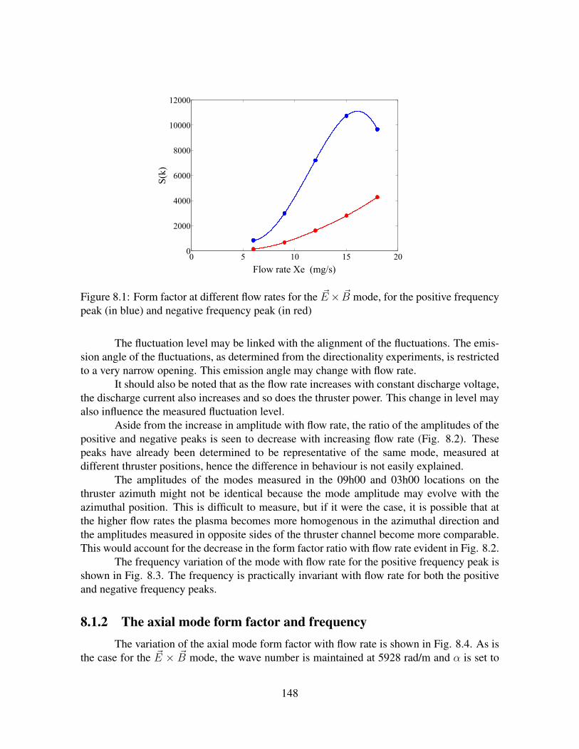
0 5 10 15 200
2000
4000
6000
8000
10000
12000
S(k)
Flow rate Xe (mg/s)
Figure 8.1: Form factor at different flow rates for the ~E× ~B mode, for the positive frequencypeak (in blue) and negative frequency peak (in red)
The fluctuation level may be linked with the alignment of the fluctuations. The emis-sion angle of the fluctuations, as determined from the directionality experiments, is restrictedto a very narrow opening. This emission angle may change with flow rate.
It should also be noted that as the flow rate increases with constant discharge voltage,the discharge current also increases and so does the thruster power. This change in level mayalso influence the measured fluctuation level.
Aside from the increase in amplitude with flow rate, the ratio of the amplitudes of thepositive and negative peaks is seen to decrease with increasing flow rate (Fig. 8.2). Thesepeaks have already been determined to be representative of the same mode, measured atdifferent thruster positions, hence the difference in behaviour is not easily explained.
The amplitudes of the modes measured in the 09h00 and 03h00 locations on thethruster azimuth might not be identical because the mode amplitude may evolve with theazimuthal position. This is difficult to measure, but if it were the case, it is possible that atthe higher flow rates the plasma becomes more homogenous in the azimuthal direction andthe amplitudes measured in opposite sides of the thruster channel become more comparable.This would account for the decrease in the form factor ratio with flow rate evident in Fig. 8.2.
The frequency variation of the mode with flow rate for the positive frequency peak isshown in Fig. 8.3. The frequency is practically invariant with flow rate for both the positiveand negative frequency peaks.
8.1.2 The axial mode form factor and frequencyThe variation of the axial mode form factor with flow rate is shown in Fig. 8.4. As is
the case for the ~E × ~B mode, the wave number is maintained at 5928 rad/m and α is set to
148

0 5 10 15 200
1
2
3
4
5
6
S(k) ratio
Flow rate Xe (mg/s)
Figure 8.2: Form factor ratio of positive frequency peak to the negative frequency peak atdifferent flow rates for the ~E × ~B mode
0 5 10 15 200
1
2
3
4
5
6x 10
6
Frequency (Hz)
Flow rate Xe (mg/s)
Figure 8.3: Frequency of the ~E × ~B mode with flow rate (positive frequency peak)
149
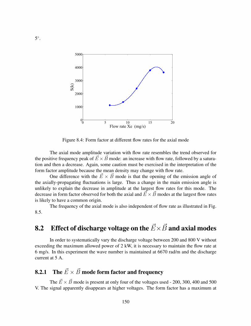
5.
0 5 10 15 200
1000
2000
3000
4000
5000
S(k)
Flow rate Xe (mg/s)
Figure 8.4: Form factor at different flow rates for the axial mode
The axial mode amplitude variation with flow rate resembles the trend observed forthe positive frequency peak of ~E× ~B mode: an increase with flow rate, followed by a satura-tion and then a decrease. Again, some caution must be exercised in the interpretation of theform factor amplitude because the mean density may change with flow rate.
One difference with the ~E × ~B mode is that the opening of the emission angle ofthe axially-propagating fluctuations is large. Thus a change in the main emission angle isunlikely to explain the decrease in amplitude at the largest flow rates for this mode. Thedecrease in form factor observed for both the axial and ~E× ~B modes at the largest flow ratesis likely to have a common origin.
The frequency of the axial mode is also independent of flow rate as illustrated in Fig.8.5.
8.2 Effect of discharge voltage on the ~E× ~B and axial modesIn order to systematically vary the discharge voltage between 200 and 800 V without
exceeding the maximum allowed power of 2 kW, it is necessary to maintain the flow rate at6 mg/s. In this experiment the wave number is maintained at 6670 rad/m and the dischargecurrent at 5 A.
8.2.1 The ~E × ~B mode form factor and frequency
The ~E × ~B mode is present at only four of the voltages used - 200, 300, 400 and 500V. The signal apparently disappears at higher voltages. The form factor has a maximum at
150
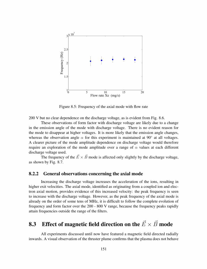
0 5 10 15 201
1.5
2
2.5
3x 10
7
Frequency (Hz)
Flow rate Xe (mg/s)
Figure 8.5: Frequency of the axial mode with flow rate
200 V but no clear dependence on the discharge voltage, as is evident from Fig. 8.6.These observations of form factor with discharge voltage are likely due to a change
in the emission angle of the mode with discharge voltage. There is no evident reason forthe mode to disappear at higher voltages. It is more likely that the emission angle changes,whereas the observation angle α for this experiment is maintained at 90 at all voltages.A clearer picture of the mode amplitude dependence on discharge voltage would thereforerequire an exploration of the mode amplitude over a range of α values at each differentdischarge voltage used.
The frequency of the ~E × ~B mode is affected only slightly by the discharge voltage,as shown by Fig. 8.7.
8.2.2 General observations concerning the axial modeIncreasing the discharge voltage increases the acceleration of the ions, resulting in
higher exit velocities. The axial mode, identified as originating from a coupled ion and elec-tron axial motion, provides evidence of this increased velocity: the peak frequency is seento increase with the discharge voltage. However, as the peak frequency of the axial mode isalready on the order of some tens of MHz, it is difficult to follow the complete evolution offrequency and form factor over the 200 - 800 V range, because the frequency peaks rapidlyattain frequencies outside the range of the filters.
8.3 Effect of magnetic field direction on the ~E × ~B modeAll experiments discussed until now have featured a magnetic field directed radially
inwards. A visual observation of the thruster plume confirms that the plasma does not behave
151

0 100 200 300 400 500 600 700 8000
1000
2000
3000
4000
5000
S(k)
Discharge voltage (V)
Figure 8.6: Form factor of the ~E × ~B mode with discharge voltage (positive frequency peak)
0 100 200 300 400 500 600 700 8000
1
2
3
4
5
x 106
Fre
quen
cy (
Hz)
Discharge voltage (V)
Figure 8.7: Frequency of the ~E × ~B mode with discharge voltage (positive frequency peak)
152
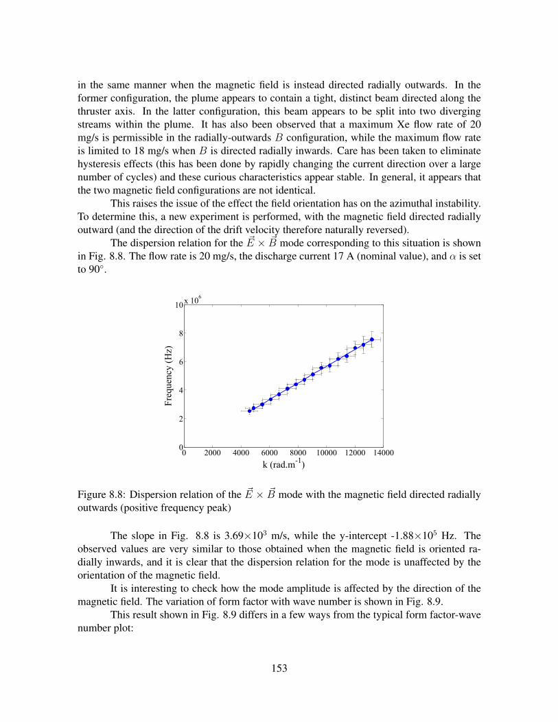
in the same manner when the magnetic field is instead directed radially outwards. In theformer configuration, the plume appears to contain a tight, distinct beam directed along thethruster axis. In the latter configuration, this beam appears to be split into two divergingstreams within the plume. It has also been observed that a maximum Xe flow rate of 20mg/s is permissible in the radially-outwards B configuration, while the maximum flow rateis limited to 18 mg/s when B is directed radially inwards. Care has been taken to eliminatehysteresis effects (this has been done by rapidly changing the current direction over a largenumber of cycles) and these curious characteristics appear stable. In general, it appears thatthe two magnetic field configurations are not identical.
This raises the issue of the effect the field orientation has on the azimuthal instability.To determine this, a new experiment is performed, with the magnetic field directed radiallyoutward (and the direction of the drift velocity therefore naturally reversed).
The dispersion relation for the ~E × ~B mode corresponding to this situation is shownin Fig. 8.8. The flow rate is 20 mg/s, the discharge current 17 A (nominal value), and α is setto 90.
0 2000 4000 6000 8000 10000 12000 140000
2
4
6
8
10x 10
6
Frequency (Hz)
k (rad.m-1)
Figure 8.8: Dispersion relation of the ~E × ~B mode with the magnetic field directed radiallyoutwards (positive frequency peak)
The slope in Fig. 8.8 is 3.69×10³ m/s, while the y-intercept -1.88×10⁵ Hz. Theobserved values are very similar to those obtained when the magnetic field is oriented ra-dially inwards, and it is clear that the dispersion relation for the mode is unaffected by theorientation of the magnetic field.
It is interesting to check how the mode amplitude is affected by the direction of themagnetic field. The variation of form factor with wave number is shown in Fig. 8.9.
This result shown in Fig. 8.9 differs in a few ways from the typical form factor-wavenumber plot:
153

0 2000 4000 6000 8000 10000 12000 14000103
104
105
106
S(k)
k (rad.m-1)
Figure 8.9: Form factor of the ~E× ~B mode with the magnetic field directed radially outwards(positive frequency peak)
• as the wave number is decreases, the mode amplitude shows significant jumps, ratherthan a smooth increase; the magnitude of these jumps is well above the uncertainty inthe determination of S(k)
• at the smallest wave numbers (4594, 4890 rad/m), the mode amplitude increases at afaster rate than the expected exponential form
The differences between the form factor characteristics of this mode for the two fieldorientations serve as a reminder that the two orientations cannot be assumed to be perfectlysymmetric.
8.4 Effect of varying magnetic field strength on the ~E × ~B
and axial modesThe magnetic field strength is changed by varying the current in the internal and
external magnetic coils, with the discharge voltage and the discharge current kept constant.The nominal value used for the magnetic coil current during the experiments at 18 mg/s is 17A. In the region where measurements are carried out (17 mm from the thruster exit plane) acurrent of 17 A in the coils corresponds to a field strength of about 15 mT.
Variation of the field strength has certain clear consequences. The electron drift ve-locity is inversely proportional to B. During the discussion of the theoretical results for theazimuthal instability in Chapter 7, it was shown that higher values of vthe/Vd are associatedwith a broadening of the unstable lobes and a reduction in the growth rate of the instability.
154
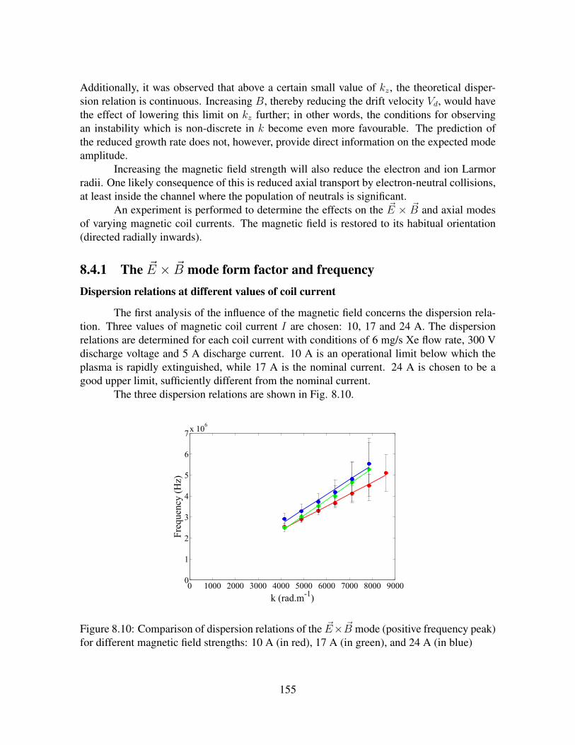
Additionally, it was observed that above a certain small value of kz, the theoretical disper-sion relation is continuous. Increasing B, thereby reducing the drift velocity Vd, would havethe effect of lowering this limit on kz further; in other words, the conditions for observingan instability which is non-discrete in k become even more favourable. The prediction ofthe reduced growth rate does not, however, provide direct information on the expected modeamplitude.
Increasing the magnetic field strength will also reduce the electron and ion Larmorradii. One likely consequence of this is reduced axial transport by electron-neutral collisions,at least inside the channel where the population of neutrals is significant.
An experiment is performed to determine the effects on the ~E × ~B and axial modesof varying magnetic coil currents. The magnetic field is restored to its habitual orientation(directed radially inwards).
8.4.1 The ~E × ~B mode form factor and frequencyDispersion relations at different values of coil current
The first analysis of the influence of the magnetic field concerns the dispersion rela-tion. Three values of magnetic coil current I are chosen: 10, 17 and 24 A. The dispersionrelations are determined for each coil current with conditions of 6 mg/s Xe flow rate, 300 Vdischarge voltage and 5 A discharge current. 10 A is an operational limit below which theplasma is rapidly extinguished, while 17 A is the nominal current. 24 A is chosen to be agood upper limit, sufficiently different from the nominal current.
The three dispersion relations are shown in Fig. 8.10.
0 1000 2000 3000 4000 5000 6000 7000 8000 90000
1
2
3
4
5
6
7x 10
6
Frequency (Hz)
k (rad.m-1)
Figure 8.10: Comparison of dispersion relations of the ~E× ~B mode (positive frequency peak)for different magnetic field strengths: 10 A (in red), 17 A (in green), and 24 A (in blue)
155

The fit parameters of the dispersion relations are shown in Eq. 8.1, where m repre-sents the slope (velocity) and c the frequency intercept.
I = 10 A, m = 3.55× 10³ m/s, c = 1.29× 10⁵ HzI = 17 A, m = 4.66× 10³ m/s, c = −6.22× 10⁵ HzI = 24 A, m = 4.40× 10³ m/s, c = −1.29× 10⁵ Hz (8.1)
There appears to be a minimal effect of the magnetic field on the frequency and dis-persion relation. It was necessary to operate at a low flow rate to cover this range of currentsand hence the signal is relatively weak and the error bars on the frequency are quite large.
These three dispersion relations of similar slopes indicate that the ~E × ~B mode, al-though related to the ~E × ~B drift, does not propagate at a velocity which is proportional tothe drift velocity E/B.
Form factor with wave number at different values of coil current
A comparison of the mode amplitudes with wave number for the three different coilcurrents is presented in Fig. 8.11. The usual exponential relationship between the energyand wave number is observed at all three currents. There is a slight variation of the overallmode amplitude with coil current at the same value of wave number. The parameters for anexponential fit of the form S(k) = Aebk are given in Eq. 8.2.
0 1000 2000 3000 4000 5000 6000 7000 8000 90002
2.5
3
3.5
4
4.5
log10[S(k)]
k (rad.m-1)
Figure 8.11: Variation of form factor with wave number of the ~E × ~B mode (positive fre-quency peak) for different magnetic field strengths: 10 A (in red), 17 A (in green), and 24 A(in blue)
156
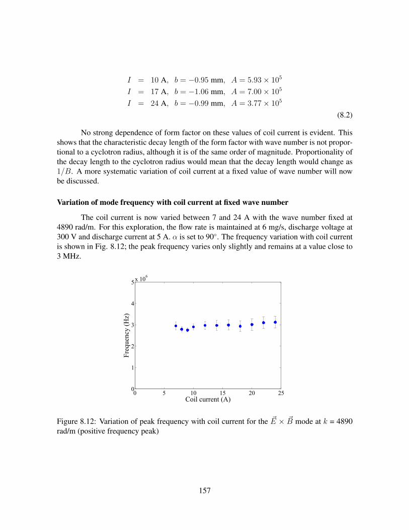
I = 10 A, b = −0.95 mm, A = 5.93× 10⁵
I = 17 A, b = −1.06 mm, A = 7.00× 10⁵
I = 24 A, b = −0.99 mm, A = 3.77× 10⁵
(8.2)
No strong dependence of form factor on these values of coil current is evident. Thisshows that the characteristic decay length of the form factor with wave number is not propor-tional to a cyclotron radius, although it is of the same order of magnitude. Proportionality ofthe decay length to the cyclotron radius would mean that the decay length would change as1/B. A more systematic variation of coil current at a fixed value of wave number will nowbe discussed.
Variation of mode frequency with coil current at fixed wave number
The coil current is now varied between 7 and 24 A with the wave number fixed at4890 rad/m. For this exploration, the flow rate is maintained at 6 mg/s, discharge voltage at300 V and discharge current at 5 A. α is set to 90. The frequency variation with coil currentis shown in Fig. 8.12; the peak frequency varies only slightly and remains at a value close to3 MHz.
0 5 10 15 20 250
1
2
3
4
5x 10
6
Frequency (Hz)
Coil current (A)
Figure 8.12: Variation of peak frequency with coil current for the ~E × ~B mode at k = 4890rad/m (positive frequency peak)
157
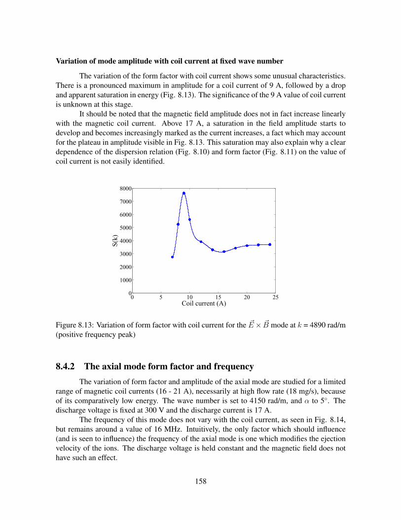
Variation of mode amplitude with coil current at fixed wave number
The variation of the form factor with coil current shows some unusual characteristics.There is a pronounced maximum in amplitude for a coil current of 9 A, followed by a dropand apparent saturation in energy (Fig. 8.13). The significance of the 9 A value of coil currentis unknown at this stage.
It should be noted that the magnetic field amplitude does not in fact increase linearlywith the magnetic coil current. Above 17 A, a saturation in the field amplitude starts todevelop and becomes increasingly marked as the current increases, a fact which may accountfor the plateau in amplitude visible in Fig. 8.13. This saturation may also explain why a cleardependence of the dispersion relation (Fig. 8.10) and form factor (Fig. 8.11) on the value ofcoil current is not easily identified.
0 5 10 15 20 250
1000
2000
3000
4000
5000
6000
7000
8000
S(k)
Coil current (A)
Figure 8.13: Variation of form factor with coil current for the ~E× ~B mode at k = 4890 rad/m(positive frequency peak)
8.4.2 The axial mode form factor and frequencyThe variation of form factor and amplitude of the axial mode are studied for a limited
range of magnetic coil currents (16 - 21 A), necessarily at high flow rate (18 mg/s), becauseof its comparatively low energy. The wave number is set to 4150 rad/m, and α to 5. Thedischarge voltage is fixed at 300 V and the discharge current is 17 A.
The frequency of this mode does not vary with the coil current, as seen in Fig. 8.14,but remains around a value of 16 MHz. Intuitively, the only factor which should influence(and is seen to influence) the frequency of the axial mode is one which modifies the ejectionvelocity of the ions. The discharge voltage is held constant and the magnetic field does nothave such an effect.
158

15 20 251
1.2
1.4
1.6
1.8
2x 10
7
Frequency (Hz)
Coil current (A)
Figure 8.14: Variation of frequency with coil current for the axial mode at k = 4150 rad/m
The form factor does show some variation with coil current, increasing gradually butnon-linearly with the coil current, as shown in Fig. 8.15.
159

15 20 250
2000
4000
6000
8000
10000
12000
S(k)
Coil current (A)
Figure 8.15: Variation of form factor with coil current for the axial mode at k = 4150 rad/m
160

In general, the frequency of the ~E× ~B mode is robust and independent of the thrusterparameters explored in this chapter. The amplitude of this mode, however, varies quite signif-icantly with the different parameters. Based on the observations of this chapter, if anomalouselectron transport is proportional to the ~E × ~B mode amplitude, then a reduction of suchtransport would require that the thruster be operated in a low flow rate (6 to 10 mg/s), highcoil current (above 14 A) regime. Such considerations should naturally be balanced withthrust requirements, for example.
The axial mode has a smaller amplitude than the ~E × ~B mode at a similar wavenumber and is only weakly influenced by changes in the thruster parameters (save for theaccelerating voltage). The influence of the discharge voltage on the ~E × ~B mode is not easyto interpret and the thruster is known to dramatically change its operating regime outside thenominal operating voltage of around 300 V.
The interplay of all these factors makes any definite recommendations for thrusteroperation premature. Instead, the relationship between the observed fluctuation characteris-tics for different thruster operating parameters and electron mobility should be investigatedin future dedicated experiments.
8.5 Low frequency signal characteristics
8.5.1 Significance of low frequency modesThe presence of low frequency oscillations (below 1 MHz) in the Hall thruster is a
widely-known and discussed phenomenon. A short description of some of the main lowfrequency oscillations was presented in the introduction. Many of these low frequency oscil-lations, such as the breathing mode and oscillations resulting from the transit time of the ionspecies, have been described in detail in the literature. Other low frequency modes, seen asdensity concentrations travelling azimuthally, have also been identified. What is common toall these studies is that they describe low frequency oscillations of length scales typically onthe order of a few cm or several mm. It is interesting to examine low frequency oscillationsmeasured at the much shorter length scales of this collective scattering study (0.48 to 1.57mm) and determine if and how they are influenced by thruster parameters.
8.5.2 Nature of low frequency signalsThe normalization procedure applied to the spectra is particularly important for the
identification of low frequency signals originating from the plasma. There are several sourcesof parasitic low frequency signals in the surroundings. Normalization is necessary to distin-guish the low frequency plasma oscillations, which have very low amplitudes, from the noise.On the raw spectra, the low frequency signals seen originate from three principal sources:
• Diffraction: diffraction on a mirror surface causes a signal peak to appear at the carrierfrequency (i.e. 0 MHz on the spectra). Such a peak is visible in the PL + LO, PL +PB + LO and PB + LO records and is removed or attenuated in the normalized
161

signal. The width and amplitude of signal peaks due to stray diffraction has beengreatly reduced on PRAXIS-II in comparison with PRAXIS-I.
• Background vibrations: weak vibrations in the surroundings occur due to the presenceof the vacuum pumps, resulting in low frequency vibrations of the optical bench. Thecorresponding signals are present in the PL + LO, PL + PB + LO and PB + LOrecords and are removed in the normalized signals.
• Plasma coupling to electronics: some plasma oscillations are strong enough to radiateand be detected directly by the electronics circuit, without the need for collective scat-tering. This observation was made during the first collective scattering trial (Chapter1). Such signals are present in both PL + LO and PL + PB + LO records (Fig.8.16). The net amplitude of this oscillation, as detected by collective scattering only, isobtained after normalization.
• Low amplitude plasma oscillations: these signals appear only in the PL + PB + LOrecord.
Fig. 8.16 shows the raw spectra obtained which illustrate some of the typical lowfrequency observations. A signal is detected in both PL+ LO and PL+ PB + LO recordsat ± 26 kHz, due to an oscillation detected by the circuit, and greatly attenuated after nor-malization. At -61 kHz, a large amplitude signal obtained by collective scattering is evident.The experimental conditions used are a flow rate of 18 mg/s and discharge voltage of 300 V.α is 90 and the wave number is 10373 rad/m.
-1.5 -1 -0.5 0 0.5 1 1.5
x 105
0
1
2
3
4
5
x 10-10
Frequency (Hz)
Signal amplitude (arbitrary units)
PL+PB+LO
PL+LO
PB+LO
Figure 8.16: Raw low frequency spectra illustrating plasma oscillations detected by the circuitand by collective scattering.
The low frequency signals on the spectra typically have irregular profiles, thus toidentify a peak frequency 〈f〉 for a particular peak, the following form is used
162
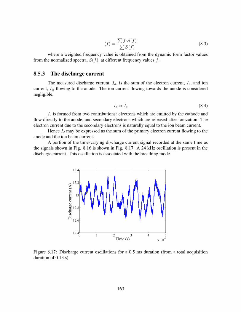
〈f〉 =
∑f ·S(f)∑S(f)
(8.3)
where a weighted frequency value is obtained from the dynamic form factor valuesfrom the normalized spectra, S(f), at different frequency values f .
8.5.3 The discharge currentThe measured discharge current, Id, is the sum of the electron current, Ie, and ion
current, Ii, flowing to the anode. The ion current flowing towards the anode is considerednegligible,
Id ≈ Ie (8.4)
Ie is formed from two contributions: electrons which are emitted by the cathode andflow directly to the anode, and secondary electrons which are released after ionization. Theelectron current due to the secondary electrons is naturally equal to the ion beam current.
Hence Id may be expressed as the sum of the primary electron current flowing to theanode and the ion beam current.
A portion of the time-varying discharge current signal recorded at the same time asthe signals shown in Fig. 8.16 is shown in Fig. 8.17. A 24 kHz oscillation is present in thedischarge current. This oscillation is associated with the breathing mode.
0 1 2 3 4 5
x 10-4
12.4
12.6
12.8
13
13.2
13.4
Time (s)
Discharge current (A)
Figure 8.17: Discharge current oscillations for a 0.5 ms duration (from a total acquisitionduration of 0.13 s)
163
8.5.4 Random appearance of low frequency signalsThe low frequency signals usually vary from record to record. That is to say, even for
identical experimental and thruster conditions, low frequency peaks of different frequenciesand amplitudes are seen. Fig. 8.18(a) and Fig. 8.18(b) illustrate the random appearance andcharacter of low frequency peaks. In the experiment shown, α = 90, the Xe flow rate 18 mg/sand the wave number 10373 rad/m, for both cases. The discharge voltage is 300 V. The onlydifference between the two cases is that the two records were made several minutes apart.Only the ± 200 kHz range is shown for both figures as all important low frequency signalstended to fall in this range.
The main frequency peaks in Fig. 8.18(a) are at -169 and -61 kHz; in contrast, the lowfrequency peaks in Fig. 8.18(b) are located at -88, 25 and 21 kHz (with a resolution of 1.5kHz). In addition, the amplitudes of the observed peaks are much larger in the second case(the maximum dynamic form factor in Fig. 8.18(a) is only 3×10⁻³ s, while in Fig. 8.18(b),in which the maximum is not shown, the maximum amplitude is 0.4 s.
The apparent random nature of the signals complicates analysis of low frequencytrends. As the frequencies and amplitudes are seen to vary for identical conditions, it is oftenunclear whether when one parameter is varied, the peak observed is a shift of the same modefrom an original frequency or the spontaneous appearance of another type of oscillation.
8.5.5 Low frequency trendsSome attempts have been made to determine if key dependencies exist, despite the
erratic nature of the low frequency signals.
Dispersion relations
No clear dispersion relations have yet been identified for the low frequency modesseen in this chapter. Fig. 8.19 shows the normalized superposed spectra for several valuesof wave number, for which the flow rate is 6 mg/s, α = 90, discharge voltage 300 V andmagnetic coil current 17 A.
The largest low frequency signal (in red) is seen at the smallest wave number, 4149rad/m. The characteristic peak frequency is 30 kHz. The other superposed spectra correspondto successively higher values of wave number and their signal amplitudes are lower. Theamplitudes are probably too small to be significant, but it appears that the frequency remainsthe same for different values of wave number. At higher values of wave number, exceeding7854 rad/m (spectra not shown), no low frequency signals are apparent at the same frequency.
Effect of flow rate
A comparison of the low frequency normalized spectra at different flow rates, from 6to 18 mg/s, is shown in Fig. 8.20. In this example, α = 90, with the wave number fixed at5928 rad/m. The discharge voltage is 300 V.
164
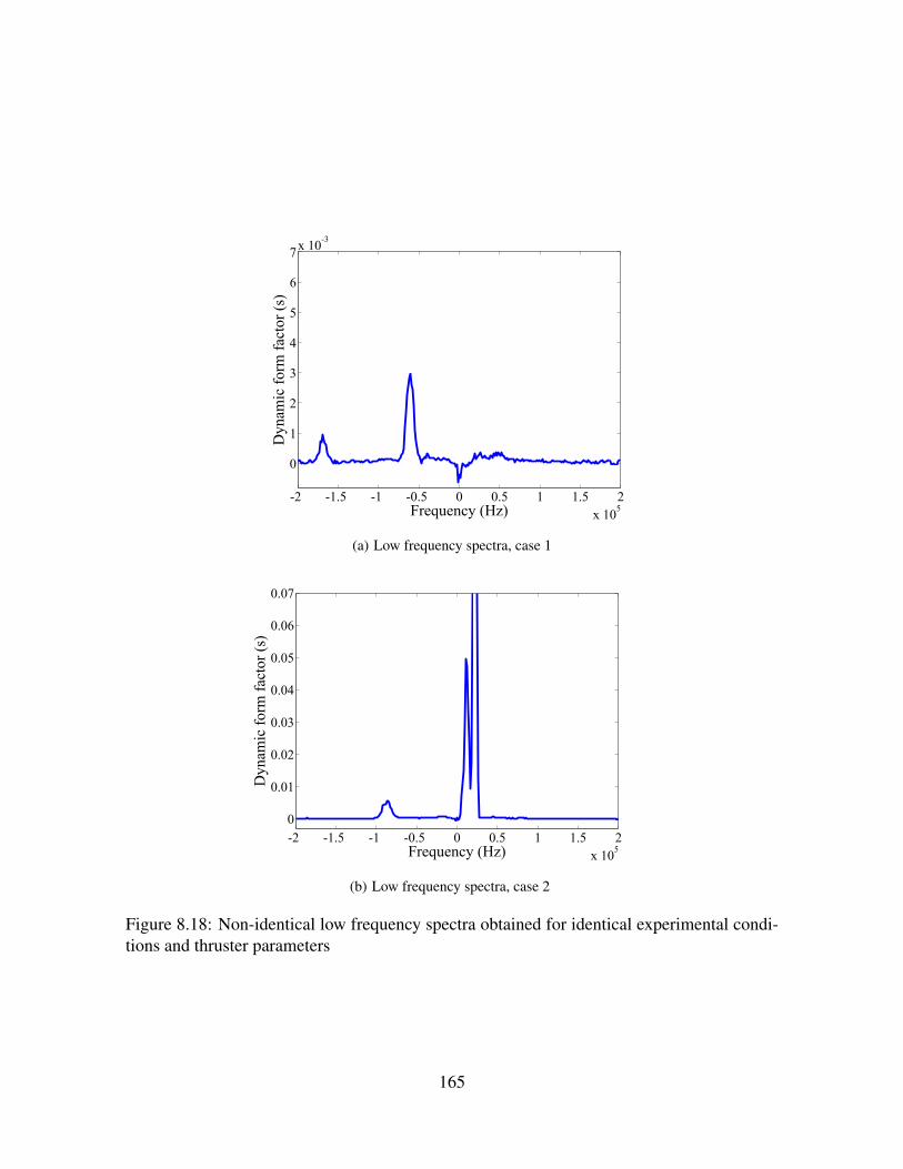
-2 -1.5 -1 -0.5 0 0.5 1 1.5 2
x 105
0
1
2
3
4
5
6
7x 10
-3
Frequency (Hz)
Dynam
ic form
fac
tor (s)
(a) Low frequency spectra, case 1
-2 -1.5 -1 -0.5 0 0.5 1 1.5 2
x 105
0
0.01
0.02
0.03
0.04
0.05
0.06
0.07
Frequency (Hz)
Dynam
ic form
fac
tor (s)
(b) Low frequency spectra, case 2
Figure 8.18: Non-identical low frequency spectra obtained for identical experimental condi-tions and thruster parameters
165

-1.5 -1 -0.5 0 0.5 1 1.5
x 105
0
0.02
0.04
0.06
0.08
0.1
0.12
Frequency (Hz)
Dynam
ic form
factor (s)
4149 rad/m
4890 rad/m
5631 rad/m
6372 rad/m
7113 rad/m
7854 rad/m
Figure 8.19: Low frequency normalized spectra at different wave numbers, with α=90
-1.5 -1 -0.5 0 0.5 1 1.5
x 105
0
2
4
6
8
10
12
14
16
x 10-3
Frequency (Hz)
Dynam
ic form
fac
tor (s)
6 mg/s
9 mg/s
12 mg/s
15 mg/s
18 mg/s
Figure 8.20: Low frequency normalized spectra at different flow rates, with α=90 and k =5928 rad/m
166

As is evident from Fig. 8.20, no clear trend in either frequency or form factor isidentifiable with flow rate. The large peak apparent at very low frequency (6 kHz) is mostlikely a diffraction residue which was not removed after normalization. The maximum staticform factor is about 80 for this mode.
-1.5 -1 -0.5 0 0.5 1 1.5
x 105
0
0.005
0.01
0.015
0.02
0.025
0.03
0.035
Frequency (Hz)
Dynam
ic f
orm
fac
tor
(s)
6 mg/s
9 mg/s
12 mg/s
15 mg/s
18 mg/s
Figure 8.21: Low frequency normalized spectra at different flow rates, with α=0
A qualitative comparison of these results may be made with the case for which thewave vector is oriented nearly parallel to the thruster axis. Fig. 8.21 shows the low fre-quency spectra obtained at different flow rates when α = 5. The flow rate is 18 mg/s and thedischarge voltage 300 V. Some low frequency signals are observed in this case at frequen-cies of 23 kHz and 73 kHz, with respective static form factor values of about 170 and 270respectively.
Effect of magnetic field strength
In this experiment, ~k is oriented parallel to ~E × ~B and the flow rate is maintained at6 mg/s, with the wave number fixed at 4890 rad/m. The magnetic field strength is varied byvarying the coil current from values of 7 to 24 A.
At high values of magnetic field coil current (20 to 24 A), no low frequency signal ispresent, apart from the usual diffraction peak at 0 Hz (Fig. 8.22(a)). At lower values of coilcurrent, some low frequency peaks begin to appear (Fig. 8.22(b)). At the lowest values ofthe coil current (7 to 14 A), a stable and unambiguous low frequency peak is observed, witha frequency and amplitude which appear to evolve with coil current (Fig. 8.22(c)).
This experiment is a case in which some influence of the thruster parameters on thelow frequency behaviour may exist. The frequency variation with coil current between 7 and14 A is shown in Fig. 8.23. The frequency (absolute value) of the low frequency peak is seen
167
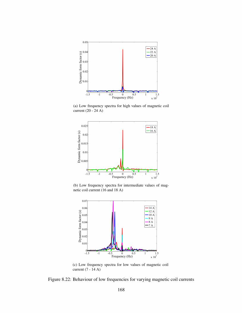
-1.5 -1 -0.5 0 0.5 1 1.5
x 105
0
0.01
0.02
0.03
0.04
0.05
Frequency (Hz)
Dynamic form factor (s)
24 A
22 A
20 A
(a) Low frequency spectra for high values of magnetic coilcurrent (20 - 24 A)
-1.5 -1 -0.5 0 0.5 1 1.5
x 105
0
0.005
0.01
0.015
0.02
0.025
Frequency (Hz)
Dynamic form factor (s)
18 A
16 A
(b) Low frequency spectra for intermediate values of mag-netic coil current (16 and 18 A)
-1.5 -1 -0.5 0 0.5 1 1.5
x 105
0
0.01
0.02
0.03
0.04
0.05
0.06
0.07
Frequency (Hz)
Dynam
ic form
fac
tor (s)
14 A
12 A
10 A
9 A
8 A
7 A
(c) Low frequency spectra for low values of magnetic coilcurrent (7 - 14 A)
Figure 8.22: Behaviour of low frequencies for varying magnetic coil currents
168

to increase as the coil current decreases. The gradual evolution and the sustained presence ofthe peak seem to support the idea that it pertains to a particular mode.
5 10 15-4.8
-4.6
-4.4
-4.2
-4
-3.8
-3.6
-3.4x 10
4
Coil current (A)
Frequency (Hz)
Figure 8.23: Frequency variation with coil current for α = 90 and k = 4890 rad/m
The frequencies, observed around -40 kHz for a wave number of 4890 rad/m, wouldcorrespond to velocities on the order of 500 m/s. This velocity is so small that it is not clearwhat thruster phenomena could produce these oscillations.
The corresponding form factor variation with coil current for the frequency peaksof Fig. 8.23 is shown in Fig. 8.24. The form factor has unusually high values (for lowfrequencies) at small coil currents, with a maximum around 8 A followed by a decrease asthe coil current increases.
8.5.6 DiscussionThe form factors of the low frequency signals are typically very small, very sel-
dom exceeding 500. This places their maximum amplitude levels three orders of magnitudesmaller than the maximum amplitude of the high frequency oscillations studied in this thesis.
It is important to note that the low frequency observations described here are notnecessarily comparable to those mentioned in other works, even though the frequencies aresimilar. The length scales accessible in our experiments do not correspond to the lengthscales of the low frequency oscillations commonly described in the literature and so no directcorrelation between the breathing mode and transit time oscillations can be described. Inthe azimuthal direction, for instance, low frequency oscillations have been measured withwavelengths on the order of the thruster circumference [13], a spatial scale well beyond thatwhich is measurable by this diagnostic.
The mechanisms by which electrons are transported to the anode appear to occur overa wide range of spatial and temporal scales. On the one hand, our results concerning the high
169
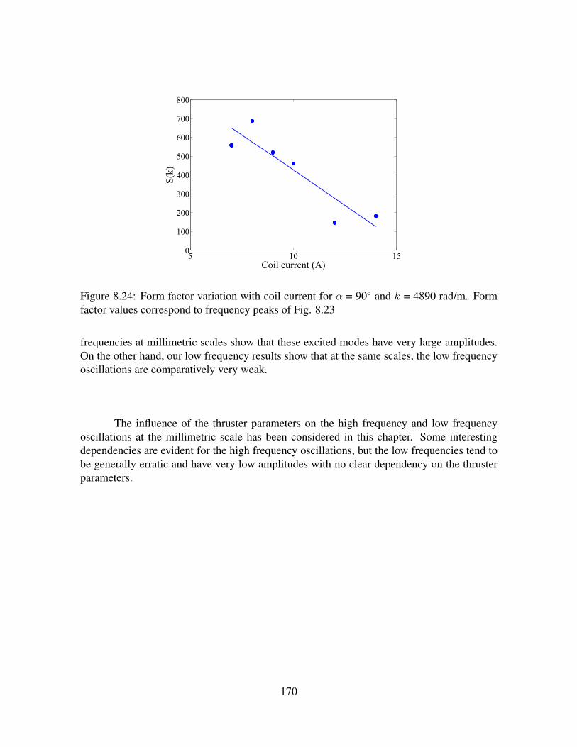
5 10 150
100
200
300
400
500
600
700
800
S(k)
Coil current (A)
Figure 8.24: Form factor variation with coil current for α = 90 and k = 4890 rad/m. Formfactor values correspond to frequency peaks of Fig. 8.23
frequencies at millimetric scales show that these excited modes have very large amplitudes.On the other hand, our low frequency results show that at the same scales, the low frequencyoscillations are comparatively very weak.
The influence of the thruster parameters on the high frequency and low frequencyoscillations at the millimetric scale has been considered in this chapter. Some interestingdependencies are evident for the high frequency oscillations, but the low frequencies tend tobe generally erratic and have very low amplitudes with no clear dependency on the thrusterparameters.
170
Chapter 9
Stability analysis of longitudinal plasmawaves
Contents9.1 Evolution of the electron distribution . . . . . . . . . . . . . . . . . . . 172
9.1.1 Vlasov equation . . . . . . . . . . . . . . . . . . . . . . . . . . . 172
9.1.2 Zeroth order solution: uniform steady-state motion . . . . . . . . . 173
9.1.3 Solution to the linearized Vlasov equation: the homogeneous equa-tion . . . . . . . . . . . . . . . . . . . . . . . . . . . . . . . . . . 174
9.1.4 Solution to the linearized Vlasov equation: the complete equation . 176
9.1.5 The integrand . . . . . . . . . . . . . . . . . . . . . . . . . . . . . 176
9.2 The first order electron distribution function . . . . . . . . . . . . . . . 177
9.3 Electron density . . . . . . . . . . . . . . . . . . . . . . . . . . . . . . . 179
9.3.1 Integration of f1 over velocity components perpendicular to ~B . . . 179
9.3.2 Expansions and developments in the limit of zero magnetic field . . 180
9.3.3 Integration over velocities parallel to ~B . . . . . . . . . . . . . . . 181
9.4 The ion density . . . . . . . . . . . . . . . . . . . . . . . . . . . . . . . . 183
9.5 The dispersion relation . . . . . . . . . . . . . . . . . . . . . . . . . . . 183
9.6 Discussion . . . . . . . . . . . . . . . . . . . . . . . . . . . . . . . . . . 184
THE plasma in a Hall thruster may be approximated as a collisionless plasma, subjected toa uniform magnetic field ~B0 parallel to the z axis and a uniform electric field ~E0 parallel
to the x axis, in a slab geometry as shown in Fig. 9.1.The magnetic pressure associated with the magnetic field (B2/2µ0) is much larger
than the kinetic plasma pressure (nkBT ). The electrons, with a small Larmor radius in com-parison to the plasma dimensions, are magnetized, while the ions are not. This chapter is
171
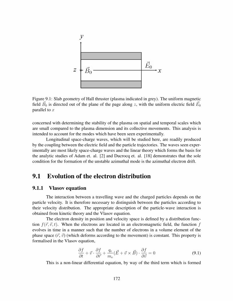
Figure 9.1: Slab geometry of Hall thruster (plasma indicated in grey). The uniform magneticfield ~B0 is directed out of the plane of the page along z, with the uniform electric field ~E0
parallel to x
concerned with determining the stability of the plasma on spatial and temporal scales whichare small compared to the plasma dimension and its collective movements. This analysis isintended to account for the modes which have been seen experimentally.
Longitudinal space-charge waves, which will be studied here, are readily producedby the coupling between the electric field and the particle trajectories. The waves seen exper-imentally are most likely space-charge waves and the linear theory which forms the basis forthe analytic studies of Adam et. al. [2] and Ducrocq et. al. [18] demonstrates that the solecondition for the formation of the unstable azimuthal mode is the azimuthal electron drift.
9.1 Evolution of the electron distribution
9.1.1 Vlasov equationThe interaction between a travelling wave and the charged particles depends on the
particle velocity. It is therefore necessary to distinguish between the particles according totheir velocity distribution. The appropriate description of the particle-wave interaction isobtained from kinetic theory and the Vlasov equation.
The electron density in position and velocity space is defined by a distribution func-tion f(~r,~v, t). When the electrons are located in an electromagnetic field, the function fevolves in time in a manner such that the number of electrons in a volume element of thephase space (~r, ~v) (which deforms according to the movement) is constant. This property isformalised in the Vlasov equation,
∂f
∂t+ ~v · ∂f
∂~r+
qeme
( ~E + ~v × ~B) · ∂f∂~v
= 0 (9.1)
This is a non-linear differential equation, by way of the third term which is formed
172

from the product of an electromagnetic field function and f , both of which depend on positionand time. To solve this equation, perturbative methods are applied.
The functions f and ~E are developed by orders, i.e.
f(~r,~v, t) = fo(~v) + f1(~r,~v, t) (9.2)~E(~r, t) = ~Eo + ~E1(~r, t) (9.3)
We consider space-charge fluctuations, which are decoupled from transverse electro-magnetic fluctuations such as magnetic field fluctuations. Thus the magnetic field containsonly the zeroth order term, ~B0. These expansions are substituted into the Vlasov equation,which must then be satisfied at every order.
The resulting equations are
( ~E0 + ~v × ~B0) · ∂f0
∂~v= 0 (9.4)
∂f1
∂t+ ~v · ∂f1
∂~r+
qeme
( ~E0 + ~v × ~B0) · ∂f1
∂~v= − qe
me
~E1 ·∂f0
∂~v(9.5)
9.1.2 Zeroth order solution: uniform steady-state motionThe solution to Eq. 9.4 is obtained via a change of variables,
~v =~E × ~B
B02 + ~u (9.6)
from which Eq. 9.4 becomes
~u× ~B · ∂f0
∂~u= 0 (9.7)
This equation is satisfied if the function f0(~u) is isotropic about the axis of ~B0. Thiscondition is fulfilled if in the crossed ~E and ~B configuration of the thruster, the electronsmove with a drift velocity ~Vd (Fig. 9.2),
~Vd =~E × ~B
B02 (9.8)
and if the distribution function of the electrons at the zeroth order is isotropic in thereference frame moving at the velocity ~Vd in the direction Oy.
f0 may be written as a shifted Maxwellian distribution
fo(~v) = no exp[−v
2x + (vy − Vd)2 + v2
z
2v2the
](9.9)
where
173
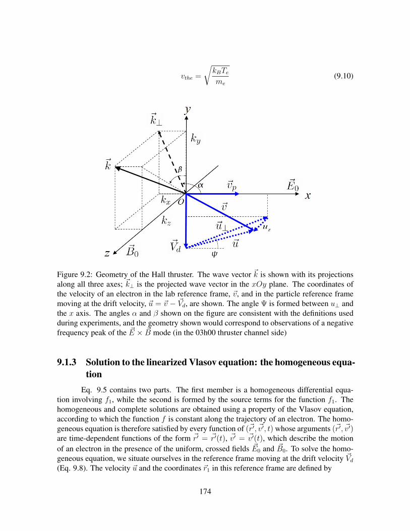
vthe =
√kBTeme
(9.10)
Figure 9.2: Geometry of the Hall thruster. The wave vector ~k is shown with its projectionsalong all three axes; ~k⊥ is the projected wave vector in the xOy plane. The coordinates ofthe velocity of an electron in the lab reference frame, ~v, and in the particle reference framemoving at the drift velocity, ~u = ~v − ~Vd, are shown. The angle Ψ is formed between u⊥ andthe x axis. The angles α and β shown on the figure are consistent with the definitions usedduring experiments, and the geometry shown would correspond to observations of a negativefrequency peak of the ~E × ~B mode (in the 03h00 thruster channel side)
9.1.3 Solution to the linearized Vlasov equation: the homogeneous equa-tion
Eq. 9.5 contains two parts. The first member is a homogeneous differential equa-tion involving f1, while the second is formed by the source terms for the function f1. Thehomogeneous and complete solutions are obtained using a property of the Vlasov equation,according to which the function f is constant along the trajectory of an electron. The homo-geneous equation is therefore satisfied by every function of (~r′, ~v′, t) whose arguments (~r′, ~v′)are time-dependent functions of the form ~r′ = ~r′(t), ~v′ = ~v′(t), which describe the motionof an electron in the presence of the uniform, crossed fields ~E0 and ~B0. To solve the homo-geneous equation, we situate ourselves in the reference frame moving at the drift velocity ~Vd(Eq. 9.8). The velocity ~u and the coordinates ~r1 in this reference frame are defined by
174
~v = ~Vd + ~u (9.11)~r = ~Vdt+ ~r1 (9.12)
With these coordinates, the first member of Eq. 9.5 gives the following homogeneousequation:
∂f1(~r1, ~u, t)
∂t+ ~u · ∂f1(~r1, ~u, t)
∂~r1
+qeme
~u× ~B0 ·∂f1(~r1, ~u, t)
∂~u= 0 (9.13)
This equation pertains to the distribution function in a uniform and steady magneticfield. The motion of electrons in this reference frame is the cyclotron motion. Let an electronbe characterised at time t by a velocity ~u, whose component ~u⊥ on the plane perpendicular to~B0 makes an angle Ψ with the axis Ox, and by a position ~r1 = (x1, y1, z1). The magnitude ofthe velocity ~u⊥ is constant, and the angle Ψ rotates in time at the electron cyclotron frequencyωce = eB0/me. The velocity and the position of the electron at time t′ < t are ~u(t′) and ~r1(t′)respectively, such that
ux(t′) = u⊥ cos [ωce(t
′ − t) + ψ] (9.14)uy(t
′) = u⊥ sin [ωce(t′ − t) + ψ] (9.15)uz(t
′) = uz (9.16)
and
r1x(t′) =
u⊥ωce
[sin [ωce(t′ − t) + ψ]− sinψ] + x1 (9.17)
r1y(t′) =
u⊥ωce
[cosψ − cos [ωce(t′ − t) + ψ] + y1 (9.18)
r1z(t′) = uz(t
′ − t) + z1 (9.19)
The velocities in the lab reference frame are obtained using Eq. 9.11,
vx(t′) = u⊥ cos [ωce(t
′ − t) + ψ] (9.20)vy(t
′) = u⊥ sin [ωce(t′ − t) + ψ] + Vd (9.21)vz(t
′) = vz = uz (9.22)
where u⊥ is defined as
u⊥ =√vx2 + (vy − Vd)2 (9.23)
and the trajectories, obtained from Eq. 9.12, are written
175

x(t′) =u⊥ωce
[sin [ωce(t′ − t) + ψ]− sinψ] + x (9.24)
y(t′) =u⊥ωce
[cosψ − cos [ωce(t′ − t) + ψ] + y + Vd(t
′ − t) (9.25)
z(t′) = vz(t′ − t) + z (9.26)
9.1.4 Solution to the linearized Vlasov equation: the complete equationEach function f(~r,~v, t) whose arguments are the trajectories given by Eq. 9.22 and
Eq. 9.25, is a solution of the homogeneous equation. The complete solution of Eq. 9.5 isobtained by the integration of the source terms over the trajectories,
fe1(~r,~v, t) = − qeme
∫ t
−∞
~E1(~r(t′), t′) · ∂fo(~v(t′))
∂~vdt′ (9.27)
Two additional properties will be used: first, the fact that the electric field is a space-charge field, and is therefore derivable from a potential φ
~E1(~r, t) = −∇φ(~r, t) (9.28)
and second, the assumption that sinusoidal functions form the basis of the solutionsto the linear differential equations. Hence
φ(~r, t) = φ ei(~k·~r−ωt) (9.29)
Thus Eq. 9.27 becomes
fe1(~r,~v, t) = iqeme
φ
∫ t
−∞
~k · ∂fo(~v(t′))
∂~vei(
~k·~r(t′)−ωt′)dt′ (9.30)
9.1.5 The integrandIntegration over the trajectory produces a projection of the gradient (in velocity space)
of the distribution function f0(~v(t′)) at the zeroth order, at time t′, over the wave vector ~k.f0(~v) depends only on the modulus of the velocity component perpendicular to the magneticfield (in the moving reference frame), u⊥, and the velocity component parallel to ~B0, vz.Thus, according to Eq. 9.9,
∂fo∂vx
(t′) = −vx(t′)
v2the
fo(u⊥, vz) (9.31)
∂fo∂vy
(t′) = −vy(t′)− Vdv2the
fo(u⊥, vz) (9.32)
∂fo∂vz
(t′) = −vz(t′)
v2the
fo(u⊥, vz) (9.33)
176

Eq. 9.30 may be written by substituting the components of velocity with the velocitydefinitions from Eq. 9.20 to Eq. 9.21, and the displacement expressions from Eq. 9.24 to Eq.9.26 into the argument of the exponential. The resulting expression is
fe1(~r,~v, t) = −i qekBTe
φfo(u⊥, vz)
∫ t
−∞dt′ ×
kxu⊥ cos [ωce[t′ − t] + ψ] + kyu⊥ sin [ωce[t
′ − t] + ψ] + kzvz ×
exp ikxu⊥ωce
[sin [ωce(t′ − t) + ψ]− sinψ] + kxx+
kyu⊥ωce
[cosψ − cos [ωce(t′ − t) + ψ]] + kyVd(t
′ − t) + kyy +
kzvz(t′ − t) + kzz − ωt′ (9.34)
In the following, polar coordinates (k⊥, θ, kz) are used for the wave vector ~k : kx =k⊥ cos θ, ky = k⊥ sin θ. In Eq. 9.34, it may be observed that the function constituting aprojection of velocity on ~k, which appears before the exponential, is the time derivative ofa part of the function constituting a projection of the position on ~k, which appears in theargument of the exponential. Thus, if the function of the position is represented by g(t), then
g(t′) = ik⊥u⊥ωcecos θ sin [ωce(t
′ − t) + ψ]−sin θ cos [ωce(t′ − t) + ψ]+kzvz(t
′−t) (9.35)
which may be written
g(t′) = i
k⊥u⊥ωce
sin [ωce(t′ − t) + ψ − θ] + kzvz(t
′ − t)
(9.36)
Hence
fe1(~r,~v, t) = − qekBTe
fo(u⊥, vz) φei(~k·~r−ωt)ei
k⊥u⊥ωce
sin (θ−ψ)
∫ t
−∞
∂g(t′)
∂t′eg(t
′)e−i(ω−~k·~Vd)(t′−t)dt′
(9.37)This form of the integrand facilitates an integration by parts.
9.2 The first order electron distribution functionIn the coefficient of the integral, an exponential of the form ei(
~k·~r−ωt) appears; thefunction f1, like the function φ, may be written in the form of a plane wave,
fe1(~r,~v, t) = fe ei(~k·~r−ωt) (9.38)
A change of variable is made in the integrand, t1 = t′ − t, and g1(t1) = g(t′) =g(t+ t1). Consequently, it becomes possible to perform an integration by parts,
177

fe = − qekBTe
fo(u⊥, vz) φeik⊥u⊥ωce
sin(θ−ψ) ×[∣∣∣eg1(t1)−i(ω−~k·~Vd)t1∣∣∣0−∞
+ i(ω − ~k · ~Vd)∫ 0
−∞eg1(t1)−i(ω−~k·~Vd)t1dt1
](9.39)
Taking into consideration the boundary conditions,
g1(t1 → −∞)→ 0 (9.40)
g1(t1 = 0) = −ik⊥u⊥ωce
sin (θ − ψ) (9.41)
The expression for fe is written as
fe = − qekBTe
fo(u⊥, vz)φ×[1 + i(ω − ~k · ~Vd)ei
k⊥u⊥ωce
sin(θ−ψ)
∫ 0
−∞dt1e
ik⊥u⊥ωce
sin (ωcet1+ψ−θ)−i(ω−~k·~Vd−kzvz)t1
](9.42)
Under this form, the integral of the time-dependent function in e(ic sin(ωcet1)) is notdirectly calculable. A development using Bessel functions is possible, however, where
eiz sinφ =∞∑
m=−∞
eimφJm(z) (9.43)
where m is an integer. Using this expression, fe may be written
fe = − qekBTe
fo(u⊥, vz)φ×
[1 + (ω − kyVd)ei
k⊥u⊥ωce
sin (θ−ψ)∞∑m
eim(ψ−θ)Jm(k⊥u⊥ωc
)
mωce − ω + kyVd + kzvz
](9.44)
This equation, with Eq. 9.38, gives the expression for the perturbation of the electrondistribution function, at the velocity ~v(v⊥, θ, vz), as a function of time, in the presence of alongitudinal wave characterized by wave vector ~k(k⊥, θ, kz), with a potential of amplitude φ.
In order to facilitate future integrations over the angle Ψ, another expansion using aBessel function in the form e(ic sin(θ−Ψ)) is used, such that
fe = − qekBTe
fo(u⊥, vz)φ
[1 + (ω − kyVd)
∞∑l
∞∑m
ei(m−l)(ψ−θ)Jl(k⊥u⊥ωce
)Jm(k⊥u⊥ωce
)
mωce − ω + kyVd + kzvz
](9.45)
This expression is very similar to that obtained by Gary and Sanderson [24] duringtheir development of the dispersion relation for shock waves propagating perpendicular to ~B.
178

9.3 Electron density
9.3.1 Integration of f1 over velocity components perpendicular to ~B
The electron density is obtained via integration over the velocities of the distributionfunction of Eq. 9.45,
ne =
∫ +∞
−∞dvz
∫ ∞0
u⊥du⊥
∫ 2π
0
fedψ (9.46)
The distribution at the zeroth order is that of Eq. 9.9 with the definition of u⊥ givenby Eq. 9.23.
The integration of Eq. 9.46 is first performed over Ψ from 0 to 2π. Due to thecylindrical symmetry of f0, only the diagonal terms (l = m) of the double summation arenon-zero,
∫ 2π
0
fedψ = −2πnoqekBTe
fo(u⊥, vz) φ
[1 + (ω − kyVd)
∞∑m
J2m(k⊥u⊥
ωce)
mωce − ω + kyVd + kzvz
](9.47)
The next step is the integration over the perpendicular velocity u⊥. The followingrelation between between Bessel functions of the first type, Jm(x), and the modified Besselfunctions In(x), is used: ∫ ∞
0
ue−u2
2 J2m(xu)du = e−x
2
Im(x2) (9.48)
thus
∫ ∞0
u⊥du⊥
∫ 2π
0
fedψ = − noqekBTe
φ1√
2πvthee− v2
z2v2the ×[
1 + (ω − kyVd)+∞∑
m=−∞
e−γIm(γ)
mωce − ω + kyVd + kzvz
](9.49)
where the argument γ is a normalization of the perpendicular wave number k⊥ by themean electron Larmor radius ρce = vthe/ωce,
γ =
(k⊥vtheωce
)2
(9.50)
An equivalent expression may be obtained from Eq. 9.47 and using the identity
+∞∑m=−∞
J2m(x) = 1 (9.51)
179

Thus
∫ ∞0
u⊥du⊥
∫ 2π
0
fedψ = − noqekBTe
φ1√
2πvthee− v2
z2v2the
+∞∑m=−∞
mωce + kzvzmωce − ω + kyVd + kzvz
e−γIm(γ)
(9.52)
9.3.2 Expansions and developments in the limit of zero magnetic fieldWhen the intensity of the magnetic field tends towards zero, it should be possible to
find the expression corresponding to the electron response in an unmagnetized plasma. Itmay also be desirable to obtain a development of this response at higher orders of B.
Some properties of modified Bessel functions
Before we proceed with the expansion, some properties of Bessel functions useful forthe analysis, taken from the handbook by Abramowitz and Stegun [1], are given below.
When B tends toward zero, the argument γ of functions Im diverge as B−2. It istherefore worth noting the asymptotic expansion of the modified Bessel function,
Im(z) ≈ ez√2πz
[1− 4m2 − 1
8z+O
(1
z2
)](9.53)
i.e.
e−γIm(γ) ≈ (2π)−1/2 ωce
k⊥vthe
[1− 4m2 − 1
8(ωce
k⊥vthe)2 + ...
](9.54)
The following other properties of modified Bessel functions and their sums will proveuseful,
I−m(z) = Im(z) (9.55)
e−z+∞∑
m=−∞
Im(z) = 1 (9.56)
e−z+∞∑
m=−∞
mIm(z) = 0 (9.57)
e−z+∞∑
m=−∞
m2Im(z) = 1 + z (9.58)
where z is real and m is an integer, and hence Im(z) ≥ 0.The parity of modified Bessel functions with respect to their index m allows the sum-
mation over the second member of Eq. 9.52 to be rewritten,
180
+∞∑m=−∞
mωce + kzvzmωce − ω + kyVd + kzvz
e−γIm(γ) =
kzvzkzvz + kyVd − ω
e−γI0(γ) + 2+∞∑m=1
kzvz(kzvz + kyVd − ω)−m2ω2ce
(kyVd + kzvz − ω)2 −m2ω2ce
e−γIm(γ) (9.59)
The limit B → 0 with a constant drift velocity
In the limit B → 0, it is necessary to define what becomes of the drift velocityVd = E0/B. If the electric field is left constant, Vd diverges asB−1 and the situation tends to-wards a non-magnetized plasma, but with an infinite drift velocity, which is not the boundarycondition we would expect to obtain. The assumption will therefore be made that E0 tendstowards zero at the same time as B, maintaining a constant drift velocity.
In this case, the summation of the second member of Eq. 9.52 is
+∞∑m=−∞
mωce + kzvzmωce − ω + kyVd + kzvz
e−γIm(γ)→
kzvzkyVd + kzvz − ω
+∞∑m=−∞
e−γIm(γ) =kzvz
kyVd + kzvz − ω(9.60)
We obtain exactly the expected response in the absence of a magnetic field, with adrift velocity.
9.3.3 Integration over velocities parallel to ~B
To obtain the electron density from the function f1 (Eq. 9.46), all that remains is theintegration of the velocities vz parallel to B,
ne =
∫ ∞−∞
dvz
∫ ∞0
du⊥u⊥
∫ 2π
0
dψfe =
− noqekBTe
φ e−γ+∞∑
m=−∞
Im(γ)
∫ ∞−∞
dvz√2πvthe
mωce + kzvzmωce − ω + kyVd + kzvz
e− v2
z2v2the (9.61)
A normalised variable ζm is defined for the frequency ω,
ζm =ω − kyVd −mωce
kzvthe√
2(9.62)
and a variable ξ for the velocity vz
ξ =vz
vthe√
2(9.63)
181
from which
mωce + kzvzmωce − ω + kyVd + kzvz
= 1 +ω − kyVdkzvthe
√2
1
ξ − ζm(9.64)
The plasma dispersion function will be used,
Z(ζ) =1√π
∫ ∞−∞
dξe−ξ
2
ξ − ζ(9.65)
With these definitions and the property from Eq. 9.56, Eq. 9.61 becomes
ne = − noqekBTe
φ
[1 +
ω − kyVdkzvthe
√2e−γ
+∞∑m=−∞
Z(ζm)Im(γ)
](9.66)
This form may also be used to write the longitudinal electron susceptibility,
χe// =1
k2~k · χe · ~k = − qe
εok2
ne
φ(9.67)
or
χe// =1
k2λ2D
[1 +
ω − kyVdkzvthe
√2e−γ
+∞∑m=−∞
Z(ζm)Im(γ)
](9.68)
where λD is the Debye length,
λD =
√εokBTenoq2
e
(9.69)
For the case of propagation purely perpendicular toB, the parallel wave vector is zero(kz = 0). Eq. 9.61 and the symmetry of the terms −m and +m of the summation are used toobtain
ne(kz = 0) = −2noqekBTe
φ e−γ∞∑m=1
Im(γ)m2
(ω−kyVdωce
)2 −m2(9.70)
This expression shows the electron cyclotron resonances with each of the harmonicsof ωce, shifted by a frequency −kyVd.
It should be noted that the function Z(ζ) takes values around ζ ≈ 0 in an interval∆ζ ≈ 1, outside of which the function decreases as ζ−1.
The argument ζm is close to zero if ω ≈ kzVd +mωce. The frequency width of the Zfunction is ∆ω ≈ kzvthe. When the direction of propagation becomes close to perpendicularto B, the frequency width ∆ω tends to zero. It is useful to compare this width to the sepa-ration ωce between two cyclotron resonances: if kzvthe < ωce, the successive resonances atfrequencies ω−kzVd = mωce are very distinct. If, in addition, this ∆ω interval is on the sameorder as the ion plasma frequency, a large ion response is expected, of the ion acoustic wave
182

type. This is the case for cyclotron waves in the thruster: each physical condition correspondsto a different series development of Eq. 9.66 or Eq. 9.68.
9.4 The ion densityThe intensity of the magnetic field in the thruster is such that the electron Larmor
radius is very small, while that of the ions is large in comparison with the thruster size. Forthis reason, the ion dynamics are described using kinetic theory in the absence of a magneticfield. The field ~E0 accelerates ions along the axis Ox. The zeroth order Vlasov equationmust take into account a velocity which depends on the x position. This spatial variationcomplicates the solution.
Taking into account the fact that the acceleration zone is short (on the order of 1 cm),the equation will not be solved in this region, but in the region immediately downstream.We will therefore assume that the ions move with a uniform velocity ~vp and parallel to Ox.The evolution of the corresponding distribution function is dictated by the linearized Vlasovequation. The longitudinal ion susceptibility is therefore
χi// = − 1
2k2λDi2Z ′(
ω − kxvpkvthi
) (9.71)
where
λDi =
√εokBTinoiq2
i
(9.72)
and Z ′(z) is the derivative of the plasma dispersion function. λDi, vthi and n0i are theion Debye length, ion thermal velocity and the ion density respectively.
9.5 The dispersion relationThe dispersion is obtained when the total space charge density
ρ = neqe + niqi (9.73)
satisfies Poisson’s equation, k2φ = ρ/εo. Since ne and ni were obtained as a functionof the potential φ, the necessary condition between the wave vector and frequency is obtained.This condition is written
1 + χe// + χi// = 0 (9.74)
That is,
1 +1
k2λ2D
[1 +
ω − kyVdkzvthe
√2e−γ
+∞∑m=−∞
Z(ζm)Im(γ)
]− 1
2k2λ2Di
Z ′(ω − kxvpkvthi
) = 0 (9.75)
183

where ζm and γ are as previously defined.
9.6 DiscussionA comparison may be made between the dispersion relation developed by Adam et.
al. [2] and whose solutions were discussed in Chapter 3 and Chapter 7, and the dispersionrelation developed here.
The dispersion relations are similar in all respects, save for the inclusion of an ionkinetic susceptibility and ion beam velocity vp in our description, which differs from a treat-ment of ions as cold and immobile. This is the source of the last term in Eq. 9.75.
Because the ions originate from different positions within the channel, the longitu-dinal dispersion of their velocities is large. Since, in addition, the angular opening of theion beam is large, the transverse dispersion of ion velocities is also large. This results in anequivalent large-temperature ion population which might induce significant changes in theinstability growth rate and instability threshold. Such an investigation of Eq. 9.75 will becompleted in future work.
184

Reflections
Experimental diagnostics provide key information on ion and electron behaviour inthe thruster, and are indispensable for understanding phenomena such as anomalous trans-port. They provide a means of improving thruster modelling efforts and identifying the idealregimes of thruster operation. There is a need for novel diagnostics which could providecomplementary information to that obtained via conventional probe methods. This work rep-resents the first application of a collective light scattering diagnostic for the study of highfrequency plasma oscillations in the Hall thruster.
The initial goals of this work were to demonstrate experimentally the presence of mil-limetric, MHz oscillations at the thruster exit which were predicted to have a role in anoma-lous electron transport. The observation of such a class of oscillations is beyond the reachof conventional diagnostics, and validation of linear kinetic theory required a completelydifferent approach. A high-performance collective scattering diagnostic, PRAXIS-I, was de-signed, built and tested for thruster studies in 2008 and provided convincing experimentalevidence that the predictions from linear kinetic theory had validity. Two different MHz-frequency modes were identified at the thruster exit: an azimuthally-propagating mode withthe predicted general characteristics, and a new, axially-propagating mode. Some interestingdifferences with theory, such as continuous dispersion relations, were also observed.
Based on the initial collective scattering results, a second phase of experiments wasperformed in 2009 with an upgraded optical bench, PRAXIS-II. The new bench enabled anumber of new investigations of the previously identified modes. In particular, localizationsof the modes and fine determinations of their directionality were performed. The azimuthalmode was discovered to propagate in three dimensions with an angular opening of only a fewdegrees, while the axially propagating mode was discovered to have an angular opening onthe order of the beam divergence angle. These new directionality experiments not only pro-vided new information on the features of the azimuthal mode, but also provided the impetusfor a re-evaluation of the three-dimensional theoretical dispersion relation. It was discoveredthat the inclusion of a wave vector component parallel to the magnetic field was sufficient toresolve many remaining key differences between linear kinetic theory and experiments.
Despite the quantity of new information and characterizations which have been madeavailable by these experiments, more interesting work remains to be done. From the theo-retical standpoint, solutions to the three-dimensional dispersion relation which incorporatethe ion velocity and temperature must be obtained. Is it possible to account for featuressuch as the directionality of the azimuthal mode by taking into account the ion dynamics and
185

damping effects? This modified dispersion relation could provide a better description of theazimuthal mode. In addition, plasma non-uniformities in the radial direction, which havebeen neglected here for simplicity, must be added to future models. It also remains to be seenwhether the azimuthal mode can play a role in thruster erosion, particularly given its lengthscales and directionality.
From the experimental standpoint, the investigations carried out on PRAXIS-II haveprovided strong reasons to expand studies of the axially-propagating mode. The next stageof experiments will attempt to increase the experimental frequency and wave number rangesfor this mode, and study more closely its link to the azimuthal mode and to the ion beamvelocity and velocity dispersion. Finally, work on quantifying anomalous electron transportand electron axial velocities is to be pursued.
186

Appendix A
Laser profilometry procedures
Laser profilometry has proven to be an indispensable tool for determining the beamquality during various stages of the optical bench construction:
• Initial laser testing: profilometry was necessary to determine the M2 value of the newlaser, a value which was stated to be typically < 1.1 by the manufacturer. In fact, theM2 value was determined to be 1.2, necessitating important modifications to the initialbench design.
• Determining diffraction reduction: the ceramic tube installed on the path of the laserbeam on PRAXIS-II was intended to absorb the long tails of the laser beam which con-tributed to excess diffraction. Profilometry was performed on the beam after the tube todetermine the effectiveness of this installation and determine an exact positioning forthe tube.
• Measurement of beam waist: a typical profilometry procedure involves the measure-ment of the laser beam waist at various locations, such as in the convergence zone infront of the thruster, and at locations where the beam size must be restricted (at thetranslator-rotator, acousto-optical deflector, etc.)
A.1 Approaches to profilometryTwo main approaches to profilometry were adopted:
• The scanning slit method: this method employs a BeamScan instrument (model 1180-FIR) from Photon Inc. This device uses a slit mounted on a spinning drum head. Thelaser beam is positioned to be incident on the window and the slit, and the radiationis transmitted to a detector. The magnitude of the transmitted signal is proportionalto the laser power and this is used to generate a beam profile. The advantage of thisdevice is that it may be used on the high power initial laser beam (about 40 W) withoutthe necessity for attenuation; the small slit size (18 µm by 9 mm) allows in only afraction of the total incident power. It is also relatively simple and requires only an
187
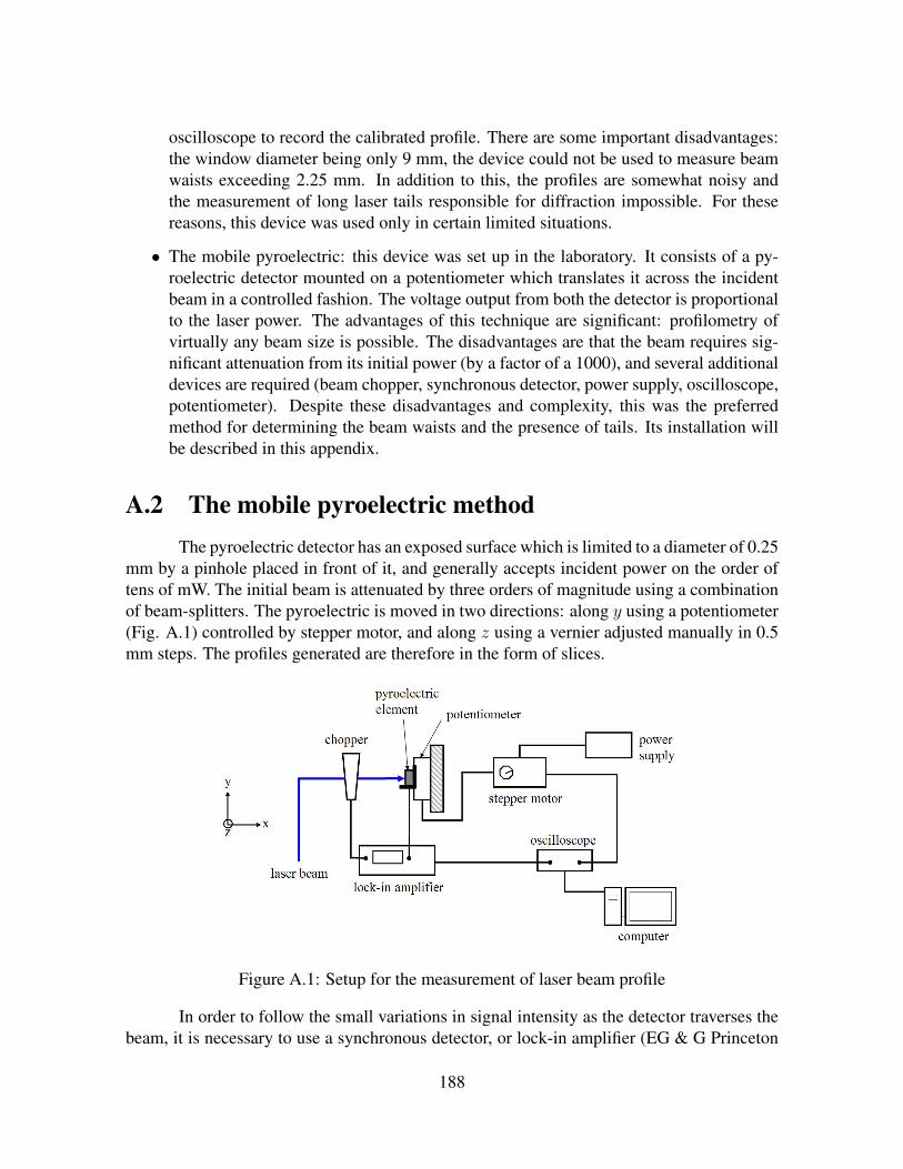
oscilloscope to record the calibrated profile. There are some important disadvantages:the window diameter being only 9 mm, the device could not be used to measure beamwaists exceeding 2.25 mm. In addition to this, the profiles are somewhat noisy andthe measurement of long laser tails responsible for diffraction impossible. For thesereasons, this device was used only in certain limited situations.
• The mobile pyroelectric: this device was set up in the laboratory. It consists of a py-roelectric detector mounted on a potentiometer which translates it across the incidentbeam in a controlled fashion. The voltage output from both the detector is proportionalto the laser power. The advantages of this technique are significant: profilometry ofvirtually any beam size is possible. The disadvantages are that the beam requires sig-nificant attenuation from its initial power (by a factor of a 1000), and several additionaldevices are required (beam chopper, synchronous detector, power supply, oscilloscope,potentiometer). Despite these disadvantages and complexity, this was the preferredmethod for determining the beam waists and the presence of tails. Its installation willbe described in this appendix.
A.2 The mobile pyroelectric methodThe pyroelectric detector has an exposed surface which is limited to a diameter of 0.25
mm by a pinhole placed in front of it, and generally accepts incident power on the order oftens of mW. The initial beam is attenuated by three orders of magnitude using a combinationof beam-splitters. The pyroelectric is moved in two directions: along y using a potentiometer(Fig. A.1) controlled by stepper motor, and along z using a vernier adjusted manually in 0.5mm steps. The profiles generated are therefore in the form of slices.
Figure A.1: Setup for the measurement of laser beam profile
In order to follow the small variations in signal intensity as the detector traverses thebeam, it is necessary to use a synchronous detector, or lock-in amplifier (EG & G Princeton
188
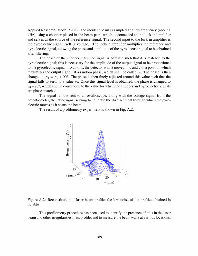
Applied Research, Model 5208). The incident beam is sampled at a low frequency (about 1kHz) using a chopper placed in the beam path, which is connected to the lock-in amplifierand serves as the source of the reference signal. The second input to the lock-in amplifier isthe pyroelectric signal itself (a voltage). The lock-in amplifier multiplies the reference andpyroelectric signal, allowing the phase and amplitude of the pyroelectric signal to be obtainedafter filtering.
The phase of the chopper reference signal is adjusted such that it is matched to thepyroelectric signal; this is necessary for the amplitude of the output signal to be proportionalto the pyroelectric signal. To do this, the detector is first moved in y and z to a position whichmaximizes the output signal, at a random phase, which shall be called p1. The phase is thenchanged to p2 = p1 + 90. The phase is then finely adjusted around this value such that thesignal falls to zero, to a value p3. Once this signal level is obtained, the phase is changed top3−90, which should correspond to the value for which the chopper and pyroelectric signalsare phase-matched.
The signal is now sent to an oscilloscope, along with the voltage signal from thepotentiometer, the latter signal serving to calibrate the displacement through which the pyro-electric moves as it scans the beam.
The result of a profilometry experiment is shown in Fig. A.2.
15
20
25 10 20 30 40
0
1
2
3
Beam intensity (V)
y (mm)
z (mm)
Figure A.2: Reconstitution of laser beam profile; the low noise of the profiles obtained isnotable
This profilometry procedure has been used to identify the presence of tails in the laserbeam and other irregularities in its profile, and to measure the beam waist at various locations.
189

A.3 Determination of the M 2 valueProfilometry using the pyroelectric detector has been essential to determining the laser
beam quality factor,M2, which provides a measure of the beam divergence and must be takeninto account during the planning of any optical bench. The M2 value is defined as the ratio ofthe beam parameter product (BPP) of the laser beam and the BPP of the laser’s fundamentaltransverse mode, identified as TEM00. The beam parameter product is defined as the productof the minimum beam diameter and the beam divergence.
The beam divergence can be determined from a far-field measurement of differentbeam waists. This cannot be done directly on the initial beam exiting the laser for two rea-sons: firstly, because the minimum beam waist is located inside the cavity and inaccessible,and secondly, because such a measurement would require determining beam waists over adistance of several metres in order to be accurate.
Instead, an artificial minimum beam waist is constructed using a lens placed at somedistance from the laser exit, after the beam has been sufficiently attenuated. The measure-ments of beam waist are then made in the regions around and far from the minimum beamwaist.
In the present example, the separation used between the laser exit and the lens is 1300mm. It is desirable to to reduce the length of the measurement region necessary by choosinga lens of short focal length. On the other hand, short focal lengths lead to smaller minimumbeam waists which are likely to saturate the detector. The lens focal length is 508 mm in thepresent case and represents a good compromise between these considerations.
Several beam profiles are recorded and fitted to a Gaussian of the form
I = I0e−(y−µ)2
2w2 (A.1)
where I0 is the signal amplitude, y the vertical position of the pyroelectric detector,µ the mean position and w the beam waist. All these parameters are optimized for the bestGaussian fit. A typical profile is shown in Fig. A.3.
The optimized values w for all distances from the lens are determined and plotted asshown in Fig. A.4. These waists are fitted to a curve of the theoretical form for the beamexpansion, a hyperbola of the form
w(z) = w0
√1 +
(z − z0
eR
)2
(A.2)
The parameters of the optimized fit - w0, z0 and eR - are determined. In the presentexample, w0 is 0.5568 mm, z0 is 710 mm and eR 65.31 mm. w0 represents the minimumbeam waist, z0 the location parameter and eR the Rayleigh length - the distance from w0 overwhich the waist increases to
√2w0.
The M2 value may now be determined.The M2 value is calculated as the ratio between the experimentally-determined beam
divergence and the theoretical divergence of a perfect Gaussian beam (of M2 value of 1).The theoretical divergence is
190
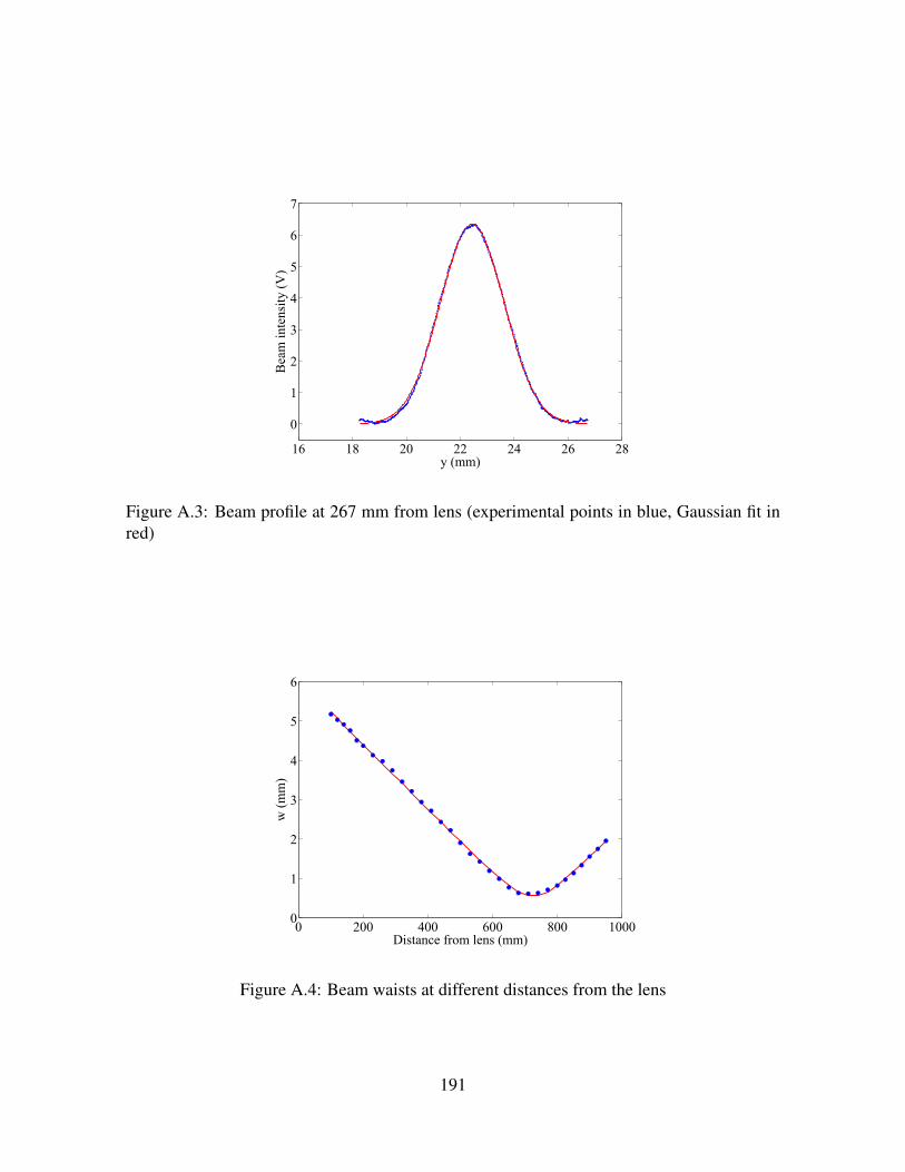
16 18 20 22 24 26 28
0
1
2
3
4
5
6
7
Beam intensity (V)
y (mm)
Figure A.3: Beam profile at 267 mm from lens (experimental points in blue, Gaussian fit inred)
0 200 400 600 800 10000
1
2
3
4
5
6
Distance from lens (mm)
w (mm)
Figure A.4: Beam waists at different distances from the lens
191
tan(θt) =λ
πw0
(A.3)
where λ is the laser wavelength. tan(θt) is 6.058×10⁻³.The experimental divergence is
tan(θe) = limz→∞
w − w0
z − z0
=w0
eR(A.4)
i.e. a value determined in the far-field region, hence the necessity for measures at alarge distance from the minimum waist, well beyond the Rayleigh length. The resulting valueof tan(θe) is 8.525×10⁻³.
The “intermediate” M2 (subject to a correction) is obtained from
M2 =tan(θe)
tan(θt)(A.5)
This value is 1.407.This must be corrected by the size of the pinhole in front of the detector; this pinhole
has a diameter of 0.25 mm, compared to the minimum waist of 0.5568 mm, which leadsto an overestimation of the waist because of the low resolution. The intermediate M2 istherefore corrected using a convolution of an “equivalent” Gaussian window based on thepinhole diameter, and the Gaussian beam.
The resulting equivalent waist of pinhole, wd, is 0.2 mm. The relation between themeasured waist w0 and the corrected waist, wt, is
wt = wm
√1 +
(wdwm
)2
(A.6)
The corrected minimum waist 0.520 mm.Finally, M2 is deduced from
M2 =πwt
2
λeR(A.7)
The value of M2 in this case is 1.2; this value was applied to the design of PRAXIS-I.
192

Appendix B
Detector efficiency
The detector used during the experiments is an HgCdTe semiconductor material ofarea 200 µm2, sensitive to wavelengths from 8 to 12 µm. It requires liquid nitrogen coolingto lower the inherent thermal noise, which is significant at room temperatures. The quantumefficiency of the detector is one factor in the determination of the absolute signal magnitudeand is defined as the ratio of the number of photons which effectively contribute to the mea-sured current, to the total number of photons incident on the detector surface. The detectorefficiency is precisely determined and used to determine the signal level.
The detector is rated for a few milliwatts of incident power, and during experiments,this power is kept below 3 mW. This also prevents saturation of the pre-amplifier.
The incident beam power is first attenuated to an acceptable level, and its level ismeasured at 0.17 mW, using a calorimeter.
The number of incident photons N corresponding to this incident power, P , is
N =P
hν(B.1)
where h is Planck’s constant, and ν = 2.83×10¹³ Hz. N is 9.07×10¹⁵.If the detector efficiency is 1, then all the incident photons contribute to the measured
current, giving rise to a maximum possible current defined as
Imax = eN(η) (B.2)
where e is the electronic charge, and η the detector efficiency. The maximum currentexpected for this incident power is 1.45 mA.
The actual current, Im, measured by the detector itself is 0.9 mA. The detector effi-ciency is then
ImImax
= 0.62 (B.3)
This value is applied during calculations of the form factor.
193

Bibliography
[1] M. Abramowitz and I. A. Stegun. Handbook of Mathematical Functions with Formulas,Graphs, and Mathematical Tables. Dover Publications, Inc., 1964.
[2] J. C. Adam, A. Heron, and G. Laval. Study of stationary plasma thrusters using two-dimensional fully kinetic simulations. Phys. Plasmas, 11(1), 2004.
[3] D. A. Alman, J. L. Rovey, R. A. Stubbers, and B. E. Jurczyc. Hall thruster electronmobility investigation using full 3D Monte Carlo trajectory simulations. In 30th Inter-national Electric Propulsion Conference, Florence, Italy, Sept. 17-20, 2007.
[4] V. I. Baranov, Yu. S. Nazarenko, V. A. Petrosov, A. I. Vasin, and Yu. M. Yashnov. Themechanism of anomalous erosion in accelerators with closed drift of electrons. In 24thInternational Electric Propulsion Conference, Moscow, Russia, IEPC-95-43, 1995.
[5] J. Bareilles. Modelisation 2D hybride d’un propulseur a effet Hall pour satellites. PhDthesis, Universite Paul Sabatier, Toulouse, 2002.
[6] E. J. Beiting, J. E. Pollard, V. Khayms, and L. Werthman. Electromagnetic emissions to60 GHz from a BPT-4000 EDM Hall thruster. In 28th International Electric PropulsionConference, 17-21 March 2003, Toulouse, France (IEPC-03-129), 2003.
[7] A. M. Bishaev and V. Kim. Local plasma properties in a Hall-current accelerator withan extended acceleration zone. Sov. Phys. Tech. Phys., 23(9), 1978.
[8] J. P. Boeuf and L. Garrigues. Low frequency oscillations in a stationary plasma thruster.J. Appl. Phys., 84(7), 1998.
[9] J. P. Bonnet, D. Gresillon, B. Cabrit, and V. Frolov. Collective light scattering as non-particle laser velocimetry. Meas. Sci. Technol., 6:620–636, 1995.
[10] A. I. Bugrova, A. V. Desyatskov, and A. I. Morozov. Electron distribution function in aHall accelerator. Sov. J. Plasma Phys., 18(8), 1992.
[11] B. Cabrit. Diffusion collective de la lumiere par un gaz turbulent: dispersionmoleculaire et turbulente. PhD thesis, Universite Paris VI, 1992.
[12] F. F. Chen. Introduction to plasma physics and controlled fusion. Plenum Press, NewYork and London, 1984.
194

[13] E. Chesta, N. B. Meezan, and M. A. Cappelli. Stability of a magnetized Hall plasmadischarge. J. Appl. Phys., 89(6), 2001.
[14] E. Y. Choueiri. Plasma oscillations in Hall thrusters. Phys. Plasmas, 8(4), 2001.
[15] F. Darnon, L. Garrigues, J. P. Boeuf, A. Bouchoule, and M. Lyszyk. Spontaneousoscillations in a Hall thruster. IEEE Transactions on Plasma Science, 27(1), February1999.
[16] P. Devynck, X. Garbet, Ph. Ghendrih, J. Gunn, C. Honore, B. Pegourie, G. Antar,A. Azeroual, P. Beyer, C. Boucher, V. Budaev, H. Capes, F. Gervais, P. Hennequin,T. Loarer, A. Quemeneur, A. Truc, and J.C. Vallet. Edge turbulence during ergodicdivertor operation in Tore supra. Nucl. Fusion, 42:697–707, 2002.
[17] A. Ducrocq. Role des instabilites electroniques de derive dans le transport electroniquedu propulseur a effet Hall. PhD thesis, Ecole Polytechnique, 2006.
[18] A. Ducrocq, J. C. Adam, A. Heron, and G. Laval. High frequency electron drift in-stability in the cross-field configuration of Hall thrusters. Phys. Plasmas, 13:102111,2006.
[19] A. Dunaevsky, Y. Raitses, and N. J. Fisch. Secondary electron emission from dielectricmaterials of a Hall thruster with segmented electrodes. Phys. Plasmas, 10(6), 2003.
[20] Yu. B. Esipchuk, A. I. Morozov, G. N. Tilinin, and A. V. Trofimov. Plasma oscillationsin closed-drift accelerators with an extended acceleration zone. Sov. Phys. Tech. Phys.,18(7), 1974.
[21] Yu. V. Esipchuk and G. N. Tilinin. Drift instability in a Hall-current plasma accelerator.Sov. Phys. Tech. Phys., 21(4), 1976.
[22] J. M. Fife. Hybrid-PIC modeling and electrostatic probe survey of Hall thrusters. PhDthesis, Massachusetts Institute of Technology, 1998.
[23] L. Garrigues, G. J. M. Hagelaar, C. Boniface, and J.-P. Boeuf. Anomalous conductivityand secondary electron emission in Hall effect thrusters. J. Appl. Phys., 100(123301),2006.
[24] S. P. Gary and J. J. Sanderson. Longitudinal waves in a perpendicular collisionlessplasma shock. i. Cold ions. J. Plasma Phys., 4:739–751, 1970.
[25] N. Gascon, M. Dudeck, and S. Barral. Wall material effects in stationary plasmathrusters. i. parametric studies of an SPT-100. Phys. Plasmas, 10:4123, 2003.
[26] D. Gawron. Phenomes de transport ionique dans le plasma d’un propulseur a effet Halla forte puissance: etude par spectroscopie laser. PhD thesis, Universite d’Orleans,2007.
195

[27] D. M. Goebel and I. Katz. Fundamentals of Electric Propulsion: Ion and HallThrusters. Jet Propulsion Laboratory, California Institute of Technology, 2008.
[28] R. J. Goldstein and W. F. Hagen. Turbulent flow measurements utilizing the Dopplershift of scattered radiation. Phys. Fluids, 10:1349–1352, 1967.
[29] D. Gresillon, C. Stern, A. Hemon, A. Truc, T. Lehner, J. Olivain, A. Quemeneur, F. Ger-vais, and Y. Lapierre. Density fluctuation measurement by far infrared light scattering.Phys. Scr., T2/2:459–466, 1982.
[30] T. J. Greytak and G. B. Benedek. Spectrum of light scattered from thermal fluctuationsin gases. Phys. Rev. Lett., 17(4), 1966.
[31] A. Guthrie and R. K. Wakerling, editors. The Characteristics of Electrical Dischargesin Magnetic Fields. McGraw-Hill Book Company, Inc., 1949.
[32] G. J. M. Hagelaar, J. Bareilles, L. Garrigues, and J. P. Boeuf. Two-dimensional modelof a stationary plasma thruster. J. Appl. Phys., 91(9), 2002.
[33] P. Hennequin, R. Sabot, C. Honore, G. T. Hoang, X. Garbet, A. Truc, C. Fenzi, andA. Quemeneur. Scaling laws of density fluctuations at high-k on Tore Supra. PlasmaPhys. Control. Fusion, 46:B121–B133, 2004.
[34] M. Hirakawa and Y. Arakawa. Numerical simulation of plasma particle behavior ina Hall thruster. In 32nd AIAA/ASME/SAE/ASEE Joint Propulsion Conference, LakeBuena Vista, FL, July 1-3 1996.
[35] E. Holzhauer and J. H. Massig. An analysis of optical mixing in plasma scatteringexperiments. Plasma Phys., 20(9), 1978.
[36] G. S. Janes and R. S. Lowder. Anomalous electron diffusion and ion acceleration in alow-density plasma. Phys. Fluids, 9(6), 1966.
[37] C. F. F. Karney. Stochastic ion heating by a lower hybrid wave. Phys. Fluids, 21(9),1978.
[38] M. Keidar and I. D. Boyd. On the magnetic mirror effect in Hall thrusters. Appl. Phys.Lett., 87:121501, 2005.
[39] A. Knoll, N. Gascon, and M. Cappelli. Numerical simulation of high frequency wavecoupling within a Hall thruster. In 43rd AIAA/ASME/SAE/ASEE Joint Propulsion Con-ference and Exhibit, 8-11 July 2007, Cincinnati, OH (AIAA 2007-5266), 2004.
[40] H. Koizumi, K. Komurasaki, and Y. Arakawa. Numerical prediction of wall erosion ona Hall thruster. Vacuum, 83:67–71, 2009.
[41] J. W. Koo and I. D. Boyd. Computational model of a Hall thruster. Computer PhysicsCommunications, 164:442–447, 2004.
196
[42] J. W. Koo and I. D. Boyd. Modeling of anomalous electron mobility in Hall thrusters.Phys. Plasmas, 13:033501, 2006.
[43] P. Lasgorceix, C. Perot, and M. Dudeck. PIVOINE ground test facility for ion thrustertesting. In Proc. Second European Spacecraft Propulsion Conference, 27-29 May, 1997.
[44] A. Lazurenko, L. Albarede, and A. Bouchoule. Physical characterization of high-frequency instabilities in Hall thrusters. Phys. Plasmas, 13:083503, 2006.
[45] A. Lazurenko, G. Coduti, S. Mazouffre, and G. Bonhomme. Dispersion relation ofhigh-frequency plasma oscillations in Hall thrusters. Phys. Plasmas, 15:034502, 2008.
[46] A. Lazurenko, T. Dudok de Wit, C. Cavoit, V. Krasnoselskikh, A. Bouchoule, andM. Dudeck. Determination of the electron anomalous mobility through measurementsof turbulent magnetic field in Hall thrusters. Phys. Plasmas, 14:033504, 2007.
[47] A. Lazurenko, V. Vial, M. Prioul, and A. Bouchoule. Experimental investigation ofhigh-frequency drifting perturbations in Hall thrusters. Phys. Plasmas, 12:013501,2005.
[48] N. Lemoine. Transport turbulent d’un plasma a travers un champ magnetique: obser-vation par diffusion collective de la lumiere. PhD thesis, Ecole Polytechnique, 2005.
[49] A. A. Litvak and N. J. Fisch. Rayleigh instability in Hall thrusters. Phys. Plasmas,11(4), 2004.
[50] A. A. Litvak, Y. Raitses, and N. J. Fisch. Experimental studies of high-frequency az-imuthal drift waves in Hall thrusters. Phys. Plasmas, 11(4), 2004.
[51] A. I. Morozov. Conditions for efficient current transport by near-wall conduction. Sov.Phys. Tech. Phys., 32(8), 1987.
[52] A. I. Morozov and V. V. Savel’ev. Theory of the near-wall conductivity. Plasma Phys.Rep., 27(7):570–575, 2001.
[53] A. I. Morozov and V. V. Savelyev. The electron dynamics in SPT-channel and theproblem of anomalous erosion. In 24th International Electric Propulsion Conference,Moscow, Russia, IEPC-95-42, 1995.
[54] A. I. Morozov and V. V. Savelyev. Fundamentals of Stationary Plasma Thruster Theory,volume 21 of Reviews of Plasma Physics. Kluwer Academic/Plenum Publishers, 2000.
[55] M. Nelkin and S. Yip. Brillouin scattering by gases as a test of the Boltzmann equation.Phys. Fluids, 9(2), 1966.
197
[56] J. Perez-Luna, G. J. M. Hagelaar, L. Garrigues, N. Dubuit, and J. P. Boeuf. Influence ofazimuthal instabilities on electron motion in a Hall effect thruster. In 30th InternationalElectric Propulsion Conference, 17-20 September 2007, Florence, Italy (IEPC-2007-124), 2007.
[57] M. Prioul. Etude experimentale des propulseurs de type Hall: processus collisionels,comportement dynamique, micro-instabilites et phenomenes de transport. PhD thesis,Universite d’Orleans, 2002.
[58] A. W. Smith and M. A. Cappelli. Investigation of field structure and electron behaviorin the near-field of Hall thrusters. In 42rd AIAA/ASME/SAE/ASEE Joint PropulsionConference and Exhibit, 9-12 July 2006, Sacramento, CA (AIAA 2006-4835), 2006.
[59] C. Stern-Forgach. Diffusion Rayleigh et detection heterodyne optique. Application auxfluctuations atmospheriques. PhD thesis, Universite Paris 11, 1981.
[60] C. A. Thomas, N. Gascon, and M. A. Cappelli. A study of the azimuthal electron drift inan ExB discharge using a non-invasive antenna array. In 39th AIAA/ASME/SAE/ASEEJoint Propulsion Conference and Exhibit, 20-23 July 2003, Huntsville, AL (AIAA 2003-4854), 2003.
[61] B. Tomchuk. Diffusion des particules transversalement au champ magnetique et diffu-sion exacerbee des ondes electromagnetiques. PhD thesis, Ecole Polytechnique, 2000.
[62] A. Truc, A. Quemeneur, P. Hennequin, D. Gresillon, F. Gervais, C. Laviron, J. Olivain,S. K. Saha, and P. Devynck. ALTAIR: An infrared laser scattering diagnostic on theTORE SUPRA tokamak. Rev. Sci. Instrum., 63(7):3716–3724, 1992.
[63] Y. Yeh and H. Z. Cummins. Localized fluid flow measurements with an He-Ne laserspectrometer. Appl. Phys. Lett., 4:176–178, 1964.
[64] D. Yu, H. Li, Z. Wu, and W. Mao. Effect of oscillating sheath on near-wall conductivityin Hall thrusters. Phys. Plasmas, 14:064505, 2007.
[65] V. V. Zhurin, H. R. Kaufman, and R. S. Robinson. Physics of closed drift thrusters.Plasma Sources Sci. Technol., 8:R1–R20, 1999.
198

Abstract
Anomalous electron transport across magnetic field lines in the Hall thruster plasma is
believed to be due in part to plasma oscillations. Oscillations of frequencies on the order of a
few megahertz and of wavelengths on the order of a millimeter have been shown to be likely
to lead to transport. Measurements of fluctuations at these length scales is, however, beyond
the reach of conventional thruster diagnostics such as probes. This work describes the first
application of a specially-designed collective light scattering diagnostic (PRAXIS) to the
measurement of electron density fluctuations and the subsequent identification of unstable
modes in the thruster plasma. Two main high frequency modes are identified, propagating
azimuthally and axially, of millimetric length scales and megahertz frequencies. The
propagation directions and angular openings of the modes are determined. The azimuthally-
propagating mode, believed to be responsible for transport, is shown to have wave vector
components antiparallel to the magnetic field and parallel to the electric field, and to
propagate within an extremely limited region. The axially-propagating mode is shown to have
features closely related to the ion beam velocity and divergence. The electron density
fluctuation level is calculated and is associated with a high electric field amplitude. The
experiments, confirming a number of predictions arising from linear kinetic theory, also
provide much additional information permitting the improvement and development of models
for both modes.
Résumé
Les oscillations dans le plasma d'un propulseur à effet Hall sont susceptibles de provoquer le
transport anormal à travers des lignes du champ magnétique. La théorie cinétique linéaire
montre qu'en particulier certaines oscillations, de fréquence de l'ordre du mégahertz et de
longueur d'onde millimétrique, peuvent jouer un rôle important dans le transport anormal. Les
échelles caractéristiques de ces fluctuations ne sont pas détectables par des outils standards
comme les sondes. Ce travail décrit pour la première fois l'utilisation d'un diagnostic de
diffusion collective (PRAXIS) conçu pour l'étude du plasma du propulseur, qui a mené à
l'identification des modes instables dans le plasma. Deux modes hautes fréquences ont été
identifiés, se propageant dans les directions azimutale et axiale, avec des longueurs d'onde
millimétriques et des fréquences de l'ordre du mégahertz. Les directions de propagation et les
ouvertures angulaires de ces modes ont été déterminées. Le mode azimutal, identifié dans la
théorie comme agent principal du transport, possède des composantes anti-parallèles au
champ magnétique et parallèles au champ électrique et se propage dans une ouverture
angulaire très restreinte. Le mode axial montre des caractéristiques liées à la vitesse et la
divergence du faisceau d'ions. Le niveau de fluctuation de la densité est associé à une grande
amplitude du champ électrique fluctuant. Les résultats des expériences sont en accord avec les
prévisions théoriques et apportent de nouvelles informations, permettant ainsi d'améliorer et
de développer des modèles pour les deux modes.