smart hvac system in university building - ruggedised.eu · smart hvac system in university...

Smart HVAC system

in University building

Nathan ZIELINSKI

Supervised by Thomas OLOFSSON and Gireesh NAIR

Abstract

The following study is part of the project RUGGEDISED. RUGGEDISED is a European project funded

under the European Union’s Horizon 2020 research and innovation programme. The idea is to combine

ICT, e-mobility and energy solutions in order to design smart and resilient cities. The three objectives of

the project are: improving the quality of life of citizens, reducing the environmental impact of activities

and creating a stimulating environment for sustainable economic development. RUGGEDISED project

brings together three lighthouse cities: Rotterdam, Glasgow and Umeå and three follower cities: Brno,

Gdansk and Parma to test, implement and accelerate the smart city model across Europe. The cities are

working in partnership with local businesses and research centres.

As one of the three lighthouse cities of RUGGEDISED project, Umeå city is developing nine smart solutions.

Umeå University and Akademiska Hus (the University property owner) are partners in four of them. This

study is a part of the smart solution U9: Demand-side management technology in a university campus. The

objective of U9 is to reduce the energy use in buildings by the implementation of energy demand

management technology. The main idea is to develop multivariate analysis tools for predictive analytics

which will support the decision process concerning tenant area use. This is the most powerful way to

reduce energy consumption by the end user. Akademiska Hus manages 3.2 million m² of area in Sweden.

The goal is to reduce the amount of bought energy by 50 % to 2025 and eliminate the CO2 footprint from

energy use in the operation of the buildings.

The following study gives an overview of a smart HVAC system based on both presence detection and time

plan control, installed in a University building. The main purpose of the research team is to compare this

smart HVAC system to a conventional one and so conclude on its performances and the saving energy

potential.

2

Table of Contents

Introduction 3

I- Case presentation 4

1.1- Building 4

1.2- Smart HVAC system 5

II- Occupancy 6

2.1- PIR sensor 6

2.2- Occupancy data and rates 7

2.3- Occupancy patterns 8

2.3.a- Space occupancy 9

2.3.b- Time occupancy 11

III- Thermal comfort and system performances 13

3.1- Smart system operation 13

3.2- Smart system performances 14

3.3- Occupants’ thermal comfort 17

IV- Energy use 18

4.1- Cooling energy use 19

4.2- Saving energy improvements 20

Conclusions and suggestions for further works 22

Main conclusions 22

Suggestions for further works 22

References 23

Annex A 24

Annex B 25

3

Introduction

Umeå is a hardly dynamic and fast-growing city in Northern Sweden. With more than 100.000

inhabitants, it is one of the twelve largest cities of the country. Umeå is a centre of education, technical

and medical research in Sweden, with two universities and over 39.000 students. Umeå University is

Sweden's fifth-oldest university (founded in 1965) and currently has 31.000 students enrolled, with 4.000

employees. The city has a continental climate with short and fairly warm summers and lengthy and

freezing winters. Thus, buildings are quite well insulated and there is a will to take advantage of the

available natural resources. Smart city thinking is at the core of Umeå city’s overall vision of continued

social, economic and environmentally sustainable growth. In the University there has been an interest for

testing and evaluating existing smart technical solutions for energy savings and smart mobility to the Umeå

campus area, and seeing how this can lead to reduced energy use, and also to increase knowledge of

human energy-related behaviours and investigating how these can be move in a more energy-smart

direction. In a partnership with the city on RUGGEDISED project, the University and its property owner

installed smart systems in University buildings to improve services to users and energy management. One

of these is a smart HVAC system based on both presence detection and time plan control. The purpose of

this system is to get closer to users’ needs and reduce the energy use of buildings.

For the last few decades, a lot of effort was put to estimate properties of building elements and adjusting

HVAC system to the building related prerequisites and constraints. Nowadays, more and more effort is put

to adjust HVAC system to both, the building and the occupants’ use. It fact, if an HVAC system has to be

designed depending on the building, its first purpose is to assure thermal comfort and air quality for

occupants. The problematic is now to get closer to users’ needs to provide a better comfort and reduce

the energy use of buildings for the whole life time of the system. Thus, a smart system, designed to respect

the building constraints and interact with the building use by its occupants seems to have all the qualities.

The main objective of the work presented in this report is to give an overview of the operation, the current

performances and the capabilities of a smart HVAC system based on both presence detection and time

plan control, installed in a University building. This study will focus on one specific floor of the equipped

building for the period from 06/05/2017 to 06/05/2018. Thanks to the dataset provided by the smart

system, we will try to answer the following questions: How does the system respond to users’ presence?

What are its current performances and its room for improvements? In what proportions is this smart

system better than a conventional one?

We will first present the study’s case and give some general information about the smart HVAC system.

Then, we will focus on presence detection and try to find some occupancy pattern. After that we will have

a look on relevant values about occupants’ thermal comfort and put on light the system’s capabilities.

Then we will show how the smart system influences the building energy use and what its performances

are. Finally, we will summarize the results and conclude on this smart HVAC system’s interest in

RUGGEDISED project.

4

I- Case presentation

The first part of this chapter presents in details the subject of the study. It gives a few essentials

information that will help to understand the operating context of the studied smart HVAC system. The

second part of this chapter presents the smart HVAC system itself and explains precisely how it works and

at what kind of information we have access to.

1.1- Building

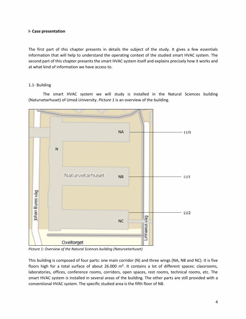
The smart HVAC system we will study is installed in the Natural Sciences building

(Naturvetarhuset) of Umeå University. Picture 1 is an overview of the building.

Picture 1: Overview of the Natural Sciences building (Naturvetarhuset)

This building is composed of four parts: one main corridor (N) and three wings (NA, NB and NC). It is five

floors high for a total surface of about 26.000 m². It contains a lot of different spaces: classrooms,

laboratories, offices, conference rooms, corridors, open spaces, rest rooms, technical rooms, etc. The

smart HVAC system is installed in several areas of the building. The other parts are still provided with a

conventional HVAC system. The specific studied area is the fifth floor of NB.

LU3

LU1

LU2

N

NC

NB

NA

5

As we can notice on Picture 1, there are two different denominations for the building’s areas: NA, NB and

NC or LU1, LU2 and LU3. The first denomination is the one used in the buildings. As an example, the first

room of the first floor of NA is named NA101. The second denomination is the one used by the smart

system (based on wings building dates and rooms’ function). As this study uses the dataset provided by

the smart system, we will exclusively use from now and for all the study the second denomination. Annex

B is a list of the rooms’ names for the studied area, based on the smart system’s denomination.

The whole studied floor is exclusively used by the organization in charge of the doctorates’ validation tests.

The floor has a restricted access and no other user can use the space. This activity is an office work and is

very close to an administrative model. Annex A is a plan of the studied floor (LU1 - floor 5) obtained from

the interaction window of the smart system. On the plan, every coloured item indicts the location of a

device from the smart HVAC system. The green ones are the exhaust air devices and the others are the

inlet air devices. This study will focus only on the inlet air devices. As we can see on the plan, the floor is

composed by two rows of offices on the sides (North and South) and some open spaces in the middle. Four

corridors serve the offices in the sides and one larger and transversal corridor in the middle serves the

common spaces (pantry, toilets and rest room). The floor contains 40 office, 3 conference rooms, 5

corridors and some other rooms with various functions. The smart system’s devices (inlet air) are

distributed everywhere in the floor with one device per office and in some other rooms for a total of 59

devices in the floor. We can notice that some rooms are not provided with any device and some other

have several devices (the transversal corridor and the pantry).

1.2- Smart HVAC system

The smart HVAC system installed in this building is a Demand Controlled Ventilation (DCV) based

on presence detection and time plan. The system controls both heating and cooling in the floor in order

to reach the set point temperature. Each inlet device control and assure the air entrance in the room.

Picture 2 is a view of an inlet air device in an office.

The inlet air goes out from the sides of the device. Each

device is provided with a few sensors: presence (in the

middle of the device), room’s temperature, supply air

flow, inlet air temperature, pressure in the inlet duct and

CO2 and exhaust air flow (only for the conference

rooms). The system is piloted by a software named

Lindinvent. It collects the sensors’ data from all the

devices and controls the actions in order to reach the set

point temperature. All the data is picked up every 10

minutes. The system can act on supply air flow and

radiators’ power. All the devices are provided by the

same air unit. Smart system’s air units are separated from

conventional ones. In wing LU3, the conventional system

provides floors one to three and the smart system

provides floors four and five. So, there are two different

air units in wing LU3. The heating system is shared with

the conventional system. Heating is provided by hot

Picture 2: View of an inlet air device in an office

6

water radiators. The hot water temperature depends only on outdoor temperature. Because of technical

design, the inlet air temperature is constant. This temperature is fixed at 16 °C all the year so we can assure

the cooling of the largest room in the hottest day.

Lindinvent system is working during standard HVAC working hours: from 6am to 6pm on working days.

During this period the system keeps rooms’ temperatures in an area of ± 1 °C around the set point

temperature. And when there is a presence detection, the system reacts to reach the set point

temperature. Graph 1 is an example of the Lindinvent cooling response for the office LA011-RC50403 on

the 06/08/2017.

Graph 1: Lindinvent cooling response for the office LA011-RC50403 on the 06/08/2017

We can see here Lindinvent’s response in real time. The set point temperature for this room is 22 °C. We

can notice a peak at 10pm that we will discuss in a further part of this study.

II- Occupancy

This part is about presence detection in the floor. We will define some occupancy patterns and show how

occupants use the floor. This part will help us to understand the system response in part III.

2.1- PIR sensor

Presence in the rooms is detected thanks to Passive Infrared sensors (PIR). As human body emits

some heat, we can detect it with the IR radiation. A PIR sensor is based on both IR radiation and movement

[1]. In fact, the sensor’s surface is divided into two parts. If one part detects an IR radiation and not the

0

5

10

15

20

25

30

35

40

45

50

22

22,5

23

23,5

24

24,5

19:12 0:00 4:48 9:36 14:24 19:12 0:00

Sup

ply

air

flo

w [

l/s]

Tem

per

atu

re [

°C]

Time

Temperature Supply Air Flow

7

other then it means that there is a heat source in movement in the area. And so, we know someone is

present in the room.

This method has its own issues. Thus, movement is required for the detection. If someone stays absolutely

motionless in front of his computer, the sensor will not detect him. Plus, as the detection is only based on

heat movement, we can have some false-positive detection. As an example, convection around radiators

or computers or air movement near a window could generate a positive detection. There is no way to

identify false-positive detection but as this study is about the system’s response, it doesn’t matter if the

detection is real or not as soon as the system reacts properly to the detection. In addition, this detection

method gives no information about the number of people or the identity. We could add other kind of

sensor to improve the detection (CO2 rate, video, etc.).

2.2- Occupancy data and rates

In the Lindinvent dataset, every time there is a positive detection the presence value takes 1 and

if not, it takes 0. As mentioned in part 1.2, the data is picked up every 10 minutes for every kind of sensors.

For a study period of one year it is more than 50.000 values per sensor. The author used MATLAB 2018 as

a data treatment software. Graph 2 is an example of the daily presence of the office LA011-RC50403 on

the 06/06/2017.

Graph 2: Daily presence of the office LA011-RC50403 on the 06/06/2017

In order to work with occupancy data, we can define two rates that will be useful regarding the data we

have access to: UR and OFz [2]. UR expresses the proportion of occupied time in a period for one zone. It

is equal to the time with presence divided by the total time of the studied period for one specific zone.

OFz expresses the proportion of occupied space in a zone at one time. In fact, we can divide a zone (the

floor) into several sub-zones (the rooms). And so OFz is equal to the number of the occupied sub-zones

divided by the total number of sub-zones in the studied zone for one specific time. In order to calculate

this second rate, we need to have access to the presence value of every rooms at a specific time. But the

dataset shows that there are some missing values. In fact, we noticed that sometimes values are spaced

out with 20 minutes or more. And as these missing values are not in the same time for every device, the

dataset’s timelines are desynchronized. So, we compared all the timelines in order to find the common

one and keep only these values. Graph 3 is the floor daily presence on the 06/11/2017.

0

0,5

1

1,5

19:12 0:00 4:48 9:36 14:24 19:12 0:00

Pre

sen

ce

Time

8

Graph 3: Floor daily presence on the 06/11/2017

We can see here the evolution of the floor use during the day. This evolution is similar to office works [3].

By dividing this evolution by the total number of devices, we obtain the evolution of the proportion of

space use (OFz) depending on time. Graph 4 is the floor weekly OFz for the week 24.

Graph 4: Floor weekly OFz for the week 24

We can easily identify here the seven days of the week and how occupants are present for each of them.

We can notice that there is some presence during week-end, but as PIR sensors don’t give information

about the identity we can’t know if there are occupants or the cleaning team or even some false-positive

detections.

2.3- Occupancy patterns

Using the two rates previously defined, we are able to study the occupancy patterns for the floor

and for each room. We have to precise that using the common timeline the loss of data is about 3 to 6 %

of the data, depending on the room, and the total loss is about 5 % which is considered acceptable for this

study’s needs.

0

10

20

30

40

50

60

19:12 0:00 4:48 9:36 14:24 19:12 0:00

Nb

r o

f p

rese

nce

Time

0,00

10,00

20,00

30,00

40,00

50,00

60,00

70,00

80,00

90,00

100,00

06-11-17 06-12-17 06-13-17 06-14-17 06-15-17 06-16-17 06-17-17 06-18-17 06-19-17 06-20-17

OFz

[%

]

Time

9

2.3.a- Space occupancy

Using OFz, we can show that the maximum occupation of the floor is 88 % during the year. This means

that at least 12 % of the space was never used during a whole year for this floor. Compared to a

conventional HVAC system which should have work whenever there was someone or not, this represents

a large saving energy potential. An interesting thing to do is to divide the floor into several parts, trying to

see if some parts are more used than some others. Picture 3 is a plan of the floor divided into four sub-

zones: A, B, C and D.

Picture 3: Plan of the floor divided into four sub-zones: A, B, C and D

The idea here is to compare the four sub-zones’ occupancy to the occupancy of the 40 offices. Table 1 is a

comparative table of the four sub-zones with their average OFzs for the year.

We can first notice that the average OFzs are very low.

This is because the averages are for the whole year,

including nights and week-ends when the floor is

unoccupied. Then we can see that zones B and D are

more occupied than zones A and C and with averages

upper the total offices’ average, despite an upper

number of offices. This means that the right part (East)

of this floor was usually more occupied than the left part

(West) during the studied year.

As this study is focused on the Lindinvent system’s capacities, we will work on the system’s corresponding

working hours. Thus, all the further time periods of this study will exclusively be based on the standard

HVAC working hours. This means that the studied year is only composed by the working days (Monday to

Friday) from 6am to 6pm. Graph 5 is the evolution of the average OFz of the floor for all the weeks of the

year (HVAC working hours).

A

D C

B

Zone OFz [%] Nbr of office

A 9,6 10

B 14,7 11

C 11,2 9

D 14,7 10

Offices 12,6 40

Table 1: Comparative table of the four sub-zones

10

Graph 5: Evolution of the average OFz of the floor for all the weeks of the year

This graph shows how the floor is used depending on the time during the whole year. We can notice three

low use periods. The first one is from weeks 27 to 31 which correspond to the summer in Sweden. The

second one is the week 52 with Christmas and the end of the year. And the last one is during weeks 18

and 19 which correspond to a national vacation time in Sweden. The average OFzs go from 2 to 48 % with

an average of 35 % for the year. Once again, compared to a conventional system which works for 100 %

of occupation all the time, the saving energy potential is far from being negligible. Graph 6 is the evolution

of the average OFz of the floor for all the months of the year.

Graph 6: Evolution of the average OFz of the floor for all the months of the year

This graph gives more information about the occupants’ use of the space during the year. We can find the

same evolution of the averages (in blue), with low occupancy periods during summer and in December. In

addition, we can see the maximum occupancies (in orange) for each month and their 90th percentile (in

0,00

10,00

20,00

30,00

40,00

50,00

60,00

70,00

80,00

90,00

100,00

23 25 27 29 31 33 35 37 39 41 43 45 47 49 51 1 3 5 7 9 11 13 15 17 19 21

OFz

[%

]

Week

0,00

10,00

20,00

30,00

40,00

50,00

60,00

70,00

80,00

90,00

100,00

Jun/17 Jul/17 Aug/17 Sep/17 Oct/17 Nov/17 Dec/17 Jan/18 Feb/18 Mar/18 Apr/18 May/18

OFz

[%

]

Month/Year

Mean 90th percentile Max

11

yellow). This last information is the value for which 90 % of the OFzs are lower. Thus, if the annual

occupancy average is 35 % we can see that it is rarely greater than 70 %.

2.3.b- Time occupancy

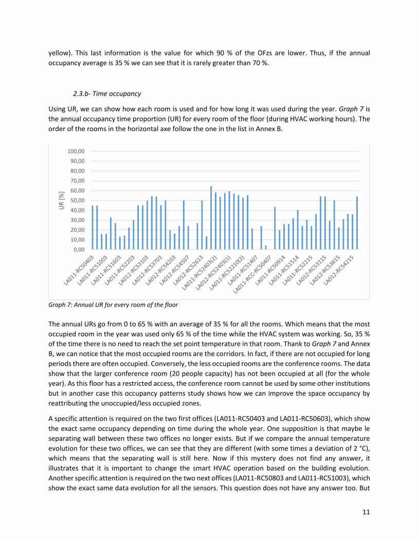
Using UR, we can show how each room is used and for how long it was used during the year. Graph 7 is

the annual occupancy time proportion (UR) for every room of the floor (during HVAC working hours). The

order of the rooms in the horizontal axe follow the one in the list in Annex B.

Graph 7: Annual UR for every room of the floor

The annual URs go from 0 to 65 % with an average of 35 % for all the rooms. Which means that the most

occupied room in the year was used only 65 % of the time while the HVAC system was working. So, 35 %

of the time there is no need to reach the set point temperature in that room. Thank to Graph 7 and Annex

B, we can notice that the most occupied rooms are the corridors. In fact, if there are not occupied for long

periods there are often occupied. Conversely, the less occupied rooms are the conference rooms. The data

show that the larger conference room (20 people capacity) has not been occupied at all (for the whole

year). As this floor has a restricted access, the conference room cannot be used by some other institutions

but in another case this occupancy patterns study shows how we can improve the space occupancy by

reattributing the unoccupied/less occupied zones.

A specific attention is required on the two first offices (LA011-RC50403 and LA011-RC50603), which show

the exact same occupancy depending on time during the whole year. One supposition is that maybe le

separating wall between these two offices no longer exists. But if we compare the annual temperature

evolution for these two offices, we can see that they are different (with some times a deviation of 2 °C),

which means that the separating wall is still here. Now if this mystery does not find any answer, it

illustrates that it is important to change the smart HVAC operation based on the building evolution.

Another specific attention is required on the two next offices (LA011-RC50803 and LA011-RC51003), which

show the exact same data evolution for all the sensors. This question does not have any answer too. But

0,00

10,00

20,00

30,00

40,00

50,00

60,00

70,00

80,00

90,00

100,00

UR

[%

]

12

as the system is reacting based on these data, we can still study the system’s reaction to the data, whatever

it seems unrealistic.

If this study is focused on the HVAC working hours, it is important to know if occupants use the floor

outside this period. Graph 8 is the annual occupancy time proportion (UR) outside the HVAC working hours

for every room of the floor.

Graph 8: Annual UR outside the HVAC working hours for every room of the floor

We can see that four rooms have an important occupancy outside the HVAC working hours. Three of them

are some technical spaces which a special function which should explain the presence outside the HVAC

working hours. The last one is an office with 23 % of the presence of the year outside the HVAC working

hours. As a reminder, the presence sensor does not give us any information about the identity of the

occupants. So, it could be the cleaning team or the technical team or anyone else who have access to the

floor.

In this part, we have seen first that the presence data could be different from the real occupancy because

of the sensors used. In addition, some information are missing (like the number of occupants or their

identity) to have a better understanding of the results. Then we have seen that the right part of the floor

seems to be more occupied. We could also identify three periods of low occupancy, corresponding to

vacations times. After that, we have seen that, for the whole year, the space occupancy of the floor is

rarely greater than 70 %, with a maximum of 88 %. That means that most of the time there is no need to

cool or heat a space which is not occupied. And finally we have seen that the annual occupancy time

proportion of the rooms is highly dependent on their function. Now all these information about occupancy

patterns will allow us to investigate the system’s capabilities.

0,00

10,00

20,00

30,00

40,00

50,00

60,00

70,00

80,00

90,00

100,00

UR

[%

]

13

III- Thermal comfort and system performances

This part is about thermal comfort and the system’s performances. We will try to set an objective definition

about the complex notion of thermal comfort. Then we will analyse some relevant results and put on the

light the smart system’s current performances and its capabilities.

3.1- Smart system operation

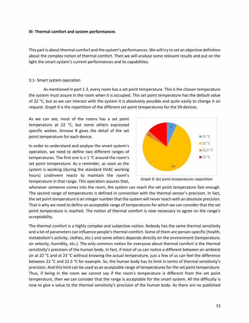
As mentioned in part 1.3, every room has a set point temperature. This is the chosen temperature

the system must assure in the room when it is occupied. This set point temperature has the default value

of 22 °C, but as we can interact with the system it is absolutely possible and quite easily to change it on

request. Graph 9 is the repartition of the different set point temperatures for the 59 devices.

As we can see, most of the rooms has a set point

temperature at 22 °C, but some others expressed

specific wishes. Annexe B gives the detail of the set

point temperature for each device.

In order to understand and analyse the smart system’s

operation, we need to define two different ranges of

temperatures. The first one is ± 1 °C around the room’s

set point temperature. As a reminder, as soon as the

system is working (during the standard HVAC working

hours) Lindinvent reacts to maintain the room’s

temperature in that range. This operation assures that,

whenever someone comes into the room, the system can reach the set point temperature fast enough.

The second range of temperatures is defined in connection with the thermal sensor’s precision. In fact,

the set point temperature is an integer number that the system will never reach with an absolute precision.

That is why we need to define an acceptable range of temperatures for which we can consider that the set

point temperature is reached. The notion of thermal comfort is now necessary to agree on the range’s

acceptability.

The thermal comfort is a highly complex and subjective notion. Nobody has the same thermal sensitivity

and a lot of parameters can influence people’s thermal comfort. Some of them are person-specific (health,

metabolism’s activity, clothes, etc.) and some others depends directly on the environment (temperature,

air velocity, humidity, etc.). The only common notion for everyone about thermal comfort is the thermal

sensitivity’s precision of the human body. In fact, if most of us can notice a different between an ambient

air at 22 °C and at 23 °C without knowing the actual temperature, just a few of us can feel the difference

between 22 °C and 22.5 °C for example. So, the human body has its limit in terms of thermal sensitivity’s

precision. And this limit can be used as an acceptable range of temperatures for the set point temperature.

Thus, if being in the room we cannot say if the room’s temperature is different from the set point

temperature, then we can consider that the range is acceptable for the smart system. All the difficulty is

now to give a value to the thermal sensitivity’s precision of the human body. As there are no published

Graph 9: Set point temperatures repartition

4

45

2

8

21 °C

22 °C

22,5 °C

23 °C

14

studies about this subject, we randomly choose the range of ± 0.5 °C around the room’s set point

temperature, based on personal feelings.

Now provided with these two ranges of temperatures, we are able to analyse the smart system’s

performances. Graph 10 is an example of the daily temperature of the office LA011-RC50403, on the

06/08/2017, provided with the two ranges previously defined.

Graph 10: Daily temperature of the office LA011-RC50403, on the 06/08/2017, provided with the two ranges

For this office, the set point temperature is 22 °C. In this graph, the area delimited by the two green lines

is the range where the room’s temperature should be during the whole HVAC working hours period. The

area delimited by the two red lines is the range where the room’s temperature should be every time

someone is present in the room. As the detailed room’s occupancy is not provided for that specific day,

we cannot compare it to the times when the room’s temperature is actually in the thermal comfort range.

3.2- Smart system performances

Now that we have set the definition of thermal comfort in connection with this smart system, we

are able to study it for the floor during the concerned year. To do this, we use the occupancy and room’s

temperature data provided by Lindinvent and compare the presence times with the deviation of the

temperature from the set point temperature for each room. Graph 11 is the annual time proportion of

thermal comfort for every room of the floor.

20,5

21

21,5

22

22,5

23

23,5

24

24,5

25

0:00 2:24 4:48 7:12 9:36 12:00 14:24 16:48 19:12 21:36

Tem

per

atu

re [

°C]

Time

15

Graph 11: Annual time proportion of thermal comfort for every room of the floor

As a reminder, we consider that there is thermal comfort if the room’s temperature is in the acceptable

range of temperatures for thermal comfort (± 0.5 °C around the set point temperature) while someone is

present in the room. Thus, this graph shows the performances of the smart system to reach the set point

temperature in link with occupancy. This is the main purpose of this smart system: assure the occupants’

thermal comfort by presence detection. The values go from 0.2 to 97 % with an average of 56 % for all the

rooms, which means that people feels comfortable only half of the time they are present. This is a very

mediocre result compared to our expectations for a smart system. Of course, these results highly depend

on the definition of thermal comfort we have set. As an example, if we consider that the acceptable range

of temperatures for thermal comfort is ± 1 °C around the set point temperature, then the average for all

the rooms becomes 83 %, which is quite better. In order to give us an idea about the acceptability of these

results, we could compare them to the time proportion of thermal comfort with a conventional HVAC

system. But this results would be highly criticisable, because based on survey about personal feelings.

Anyway, thanks to Graph 11 we can notice that some rooms have a very low time proportion of thermal

comfort, among which the four corridors that serve the offices are. This finding could be explained by a

lack of devices in these large rooms. In fact, these four corridors have only one device each. If we compare

their time proportion of thermal comfort to the one of the larger corridor which has six devices, it appears

that the number of device has a direct impact on the system capacities. In addition, it seems that the

exhaust air from offices goes directly to these corridors before leaving the floor. The conclusion is that

only one device is not enough to counterbalance the exhaust air from about ten offices. However, the

importance of the thermal comfort is relative to the room’s function. In fact, if we have showed that the

corridors are the most occupied rooms in the year, people don’t stay enough longer to feel uncomfortable.

So, in that case, the low time proportion of thermal comfort seems to be acceptable because we don’t

need it to be high. But, if we consider that each corridor is directly connected with about ten offices it

means that there is some air circulation between these corridors and the offices. In addition, if the offices’

doors are opened all the day, then the corridors’ temperature directly impact the thermal comfort in these

offices. Then the corridors’ temperature seems to be a big issue. Another problem appears here: the

repartition of the set point temperature. If we take the example of an office, with a set point temperature

at 23 °C, adjoining a corridor, with a set point temperature at 22 °C, and if we consider that the office’s

0,0010,0020,0030,0040,0050,0060,0070,0080,0090,00

100,00Th

erm

al c

om

fort

tim

e p

rop

ort

ion

[%

]

16

door is opened most of the time, then there is no way for the system to assure thermal comfort in both

rooms and it would imply a high energy use.

The two others rooms with a very low time proportion of thermal comfort are two offices (LA011-RC53503

and LA011-RC52215). We don’t know exactly why these specific offices have a low thermal comfort. One

explanation could be the repartition of the different set point temperatures in the floor. In fact, it is more

difficult to reach a specific temperature (21 °C) if all the other rooms around have a different temperature

(22 °C). But, as for every other room, the most important point is to compare the effective time proportion

of thermal comfort to the occupancy time proportion of the room. Thus we can show that if the office

LA011-RC52215 has a thermal comfort only 10 % of its presence time, this office is occupied only 24 % of

the HVAC working hours period during the whole year. So, maybe it was a specific short period when the

system could not had reach the temperatures’ range but, if the office had been occupied for a longer time

the time proportion of thermal comfort would have been greater.

We have been seeing so far the smart system’s performances to reach the acceptable range of

temperatures for the set point temperature when there is a presence detection. As a reminder, this smart

system is based on both presence detection and time plan control. Let’s focus now on its performances

about time plan control. As we have seen in parts 1.2 and 3.1, when the system is working, the room’s

temperature must be kept in the range ± 1 °C around the room’s set point temperature, whenever

someone is present or not in the room. Graph 12 is the annual time proportion of room’s temperature

outside that range for every room of the floor.

Graph 12: Annual time proportion of room’s temperature outside the ± 1 °C range for every room of the floor

This graph shows the smart system’s performances linked to its time plan control operation. Thus, we

know for every room how many times in the year the room’s temperature was outside the ± 1 °C range (in

blue). As we can see on graph 10, sometimes the room’s temperature is going in and out of a range with

small variations, which doesn’t mean that the system fails to regulate it. So, we define a second time

proportion which corresponds to the number of times when the room’s temperature is outside the ± 1°C

0,00

10,00

20,00

30,00

40,00

50,00

60,00

70,00

80,00

90,00

100,00

Tim

e p

rop

ort

ion

ou

tsid

e +/

-1

°C

[%

]

Instantaneous For at least 30 consecutive minutes

17

range for at least 30 consecutive minutes (in orange), which means that the smart system fails keeping it

in the range. As data is picked up every 10 minutes, the 30 consecutive minutes correspond to three

reactions form the smart system. We can see that there is a small difference between the two time

proportions. Once again, this graph shows the performances’ difference between the four corridors with

one device each and the one with six devices. This system’s inability to keep corridors’ temperature in the

range could explain the low time proportion of thermal comfort we have seen on Graph 11, as well as for

the office LA011-RC53503.

3.3- Occupants’ thermal comfort

Graph 11 showed the smart system’s performances to reach the thermal comfort’s range of

temperatures. If we now consider thermal comfort as occupants’ feelings and not as system’s

performances, we need to give another definition to the acceptability. In fact, as we said previously,

sometimes the room’s temperature is going in and out of the range with small variations. But, it doesn’t

mean that people feels uncomfortable every time the temperature is out of the range. So, we can define

the thermal discomfort like this: if there is someone in the room and the room’s temperature is outside

the thermal comfort’s range of temperature for at least one consecutive hour, then we can say there is

thermal discomfort. Graph 13 is the annual time proportion of thermal discomfort for every room of the

floor.

Graph 13: Annual time proportion of thermal discomfort for every room of the floor

The values go from 0 to 67 % with an average of 17 % for all the rooms. Once again, these results highly

depend on the body’s sensitivity we have chosen. Thus, if we consider that the acceptable range of

temperatures for thermal comfort is ± 1 °C around the set point temperature, then the average for all the

rooms becomes 6 %. These results are quite similar to those from Graph 11, with some exceptions. For

example, thermal discomfort for the office LA011-RC52215 is not so high compared to its very low thermal

comfort. That means most of the time the room’s temperature is not in the thermal comfort’s range, the

system can regulate it in less than an hour.

0,00

10,00

20,00

30,00

40,00

50,00

60,00

70,00

80,00

90,00

100,00

Ther

mal

dis

com

fort

tim

e [%

]

18

When we are talking about thermal discomfort, two notions are important. The first one is the discomfort

duration, illustrated by Graph 13. The second one is the deviation’s size. In fact, thermal discomfort doesn’t

have the same importance if the deviation from the set point temperature is 0.6 °C or if it is 2 °C. Graph

14 is the mean absolute deviation from the set point temperature for the time proportion of thermal

discomfort for all the rooms of the floor.

Graph 14: Mean absolute deviation from the set point temperature for all the rooms of the floor

The values go from 0.64 °C to 1.85 °C with an average of 0.97 °C for all the rooms. There are no obvious

patterns between the time proportion of thermal discomfort and the mean deviation, but we can notice

that some of the most uncomfortable rooms have the most mean deviation. Thus, corridor LA011-

RC50406 was uncomfortable almost 60 % of its presence time with a mean temperature deviation from

the set point temperature of almost 1.9 °C.

In this part, we have seen first that the freedom to choose any set point temperature is one of the biggest

advantages of this smart system compared to a conventional system. But the repartition of these set point

temperatures have to be managed in order to assure the system’s performances. Then we have seen that

thermal comfort is a highly complex notion and its definition influences the results. We have seen that

thermal comfort is lower than our expectations for a smart system. The system even fails sometimes to

regulate the temperature when there is nobody. The corridors are specially concerned by these low

performances because of both the exhaust air from offices and a lack of devices. In order to have a better

understanding of the system’s performances, we need to analyse its energy use.

IV- Energy use

This part is about energy use and system’s performances. We will try to compare the system’s energy uses

to its performances from part III and put on light some system’s operations which need improvements.

0,50

0,70

0,90

1,10

1,30

1,50

1,70

1,90

mea

n d

evia

tio

n [

°C]

19

4.1- Cooling energy use

We don’t have access to any data about the system’s energy use (both cooling and heating). But,

as we know the room’s temperature, the supply air temperature and the supply air flow every 10 minutes,

we are able to calculate the theoretical instantaneous exchange of cooling energy between the room’s air

and the supply cold air thanks to Equation 1.

Equation 1: Cooling power demand

This quantity represents the instantaneous cooling power the system needs to achieve its performances

(cooling power demand). In order to find an energy use quantity, we need to do the estimation that the

cooling power demand is constant on every 10 minutes periods. Thus, we can have an estimation of the

total cooling energy use for the whole year and for every room. These estimations on 10 minutes periods

are acceptable compared to the one year studied period. Graph 15 is the annual cooling energy demand

for all the rooms in the floor.

Graph 15: Annual cooling energy demand for all the rooms in the floor

0,00

5,00

10,00

15,00

20,00

25,00

Co

olin

g en

ergy

dem

and

[G

W.h

]

HVAC working hrs Year

∆�̇� = 𝑞�̇� . 𝜌 . 𝑐𝑝 . (𝑇𝑟𝑜𝑜𝑚 − 𝑇𝑠𝑢𝑝𝑝𝑙𝑦 𝑎𝑖𝑟)

With: ∆�̇� the cooling power [W]

𝑞�̇� the supply air flow [m3/s]

𝜌 the density [kg/m3]

𝑐𝑝 the specific heat capacity [J/kg.K]

𝑇𝑟𝑜𝑜𝑚 the room’s temperature [K]

𝑇𝑠𝑢𝑝𝑝𝑙𝑦 𝑎𝑖𝑟 the supply air’s temperature [K]

20

There are no obvious patterns between these results and the other previous graphs on this study, because

a lot of parameters can influence them. Here is a no exhaustive list of these parameters: outdoor

temperature, occupancy, size of the room, air circulation (opened door or windows) and external heating

sources (radiators, occupants, computers, solar orientation). Anyway, the main interest of Graph 15 is to

compare the cooling energy demand for the HVAC working period and the one for the whole year

(including night times and week-ends). We can see that they are different for every room, which means

the system cools when it should be off. We can estimate this overuse of cooling at 19 % of the cooling

energy demand for the HVAC working period. This observation had already be done with the peak of

supply air flow at 10pm on Graph 1, in part 1.2. In addition, the overuse of cooling is very huge for few

rooms. For now, we don’t have any explanation for that.

4.2- Saving energy improvements

The same work can be done about heating. Graph 16 is the annual time proportion of heating

outside the HVAC working period for all the rooms of the floor.

Graph 16: Annual time proportion of heating outside the HVAC working period for all the rooms of the floor

The values go from 2 to 72 % with an average of 49 % for all the rooms, which means that half of the time

the system heats, it is outside the HVAC working period, when it should be off. As we don’t have access to

any data about the heating energy use, we can’t say how much energy it represents. In fact, during these

outside periods radiators could be working at 1 % of their capacities in order to maintain a minimum

temperature in the building. However, a study about rooms’ temperature evolution during year showed

that temperatures increase during week-ends, with maximums at 25 °C. That implies that the system is

systematically cooling the floor every Monday at 6am, which is a no negligible energy use.

Keeping working on waste of energy use by the smart system, we can check if there are some times when

the system cools and heats a room at the same time. Graph 17 is the annual time proportion of

simultaneous heating and cooling for all the rooms of the floor.

0,00

10,00

20,00

30,00

40,00

50,00

60,00

70,00

80,00

90,00

100,00

Hea

tin

g o

uts

ide

HV

AC

ho

urs

[%

]

21

Graph 17: Annual time proportion of simultaneous heating and cooling for all the rooms of the floor

The values go from 1 to 95 % with an average of 57 % for all the rooms, which means that 57 % of the

HVAC working period, the system heat and cool the entire floor simultaneously. Once again, we don’t

know in what proportions the system cool or heat, so we don’t know how much energy use it represents.

But, it is a really alarming result for a smart system. In fact, it is quite obvious that cooling and heating at

the same time is far from being efficient.

In this part, we have seen first that the smart system seems to operate outside the HVAC working period.

In fact, there is a difference between the cooling energy demand for the HVAC working period and the one

for the whole year and the system heats outside the HVAC working period. We can estimate an overuse

of 19 % for the cooling. The heating doesn’t have any energy use value, but we know that half of the time

the system heats, it is outside the HVAC working period. Finally, we saw that sometimes the smart system

heats and cool a room at the same time. All these results show that there are improvements to do on this

system and there still is a part of saving energy potential.

0,00

10,00

20,00

30,00

40,00

50,00

60,00

70,00

80,00

90,00

100,00H

eati

ng

& C

oo

ling

tim

e p

rop

ort

ion

[%

]

22

Conclusions and suggestions for further works

Main conclusions:

This study gives an overview of the operation, the current performances and the capabilities of the smart

HVAC system, based on both presence detection and time plan control, installed in the Natural Sciences

Building of Umeå University, for the period from 06/05/2017 to 06/05/2018.

First, we have seen with occupancy patterns that the right part of the floor seems to be more

occupied than the left one. We also identified three periods of low occupancy, corresponding to vacations

times. We showed that for the studied period, the space occupancy of the floor is rarely greater than 70

%, with a maximum of 88 %. That means that there is a real saving energy potential thanks to presence

detection control, compared to a conventional system designed for 100 % capacities and which doesn’t

react to occupants’ presence. And we have seen that the annual occupancy time proportion of the rooms

is highly dependent on their function. Thus, the saving energy potential could be bigger if we adapt the

system operation to rooms’ functions. For example, the University has a meeting rooms booking system.

So, there is no need for the smart system to operate in conference rooms if they are not booked.

Then, we have seen that a positive aspect about this smart system is its simplicity to change control

parameters (set point temperature, basic air flow, etc.) to get closer to everybody needs. We also showed

that this freedom needs to be well manage to assure the system’s performances, like with the set point

temperatures repartition. We showed that the complex definition of thermal comfort highly influences

the results about thermal comfort. But, anyway it seems that the system’s performances are lower than

our expectations for a smart system and the system even fails sometimes to regulate the temperature

when there is nobody. The corridors are specially concerned by these low performances because of both

the exhaust air from offices and a lack of devices.

Finally, we have seen that that the smart system seems to operate outside the HVAC working

period. Or the system should be completely off during these times. Thus, the overuse of cooling energy

demand is 19 % and 49 % of the heating is outside the normal working period. In addition, we showed that

the system cools and heats at the same time for about 57 % of its working time. All these results show that

there are improvements to do on this smart system and there still is a part of saving energy potential.

Suggestions for further works:

Improve the understanding of the smart system’s operation in specific cases: exhaust air

management, finding explanations about heating and cooling outside the working period.

Perform a specific study about occupancy patterns in that floor. Specific occupancy pattern related

to specific room’s function. Comparison with occupancy patterns from other organisations.

Perform a specific study about occupants’ thermal comfort, related to studies about thermal

comfort in buildings with multivariable analysis tools.

Develop a building simulation tool, based on the actual floor’s occupancy patterns, to compare

the smart system performances to a conventional one in that specific floor.

Insert the smart system in a smart building management system to improve its performances

(opened doors / windows management)

Develop multivariable patterns with a Principal Component Analysis

23

References

[1] Halvarsson, J. (2012) Occupancy Pattern in Office Buildings - Consequences for HVAC system design and

operation, A-3 - A-4


operation, 8 – 12


operation, 103 – 108

Websites:

http://www.ruggedised.eu

https://www.lindinvent.com

24

Annex A: Plan of the studied floor (LU1 - floor 5) obtained from the interaction window of the smart system

25

Annex B: List of the rooms’ names with their nature and set point temperature

Devices Nature of the room Set point temperature [°C]

LA011-RC50403 Office 22

LA011-RC50603 Office 22,5




















LA012-RC54507 Conference room 22

LA012-RC53307 Technical space 22

LA012-RC52606 Corridor 22


LA012-RC52811 Massage 22

LA011-RC52403(1)

Corridor 22

LA011-RC52403(2)

LA011-RC52403(3)

LA011-RC52403(4)

LA012-RC52403(1)

LA012-RC52403(2)

Caption: Office

Conference room

Corridor

Other

26

LA011-RC52210(1) Pantry 22

LA011-RC52210(2)



LA011-RC51407 Technical space 22

LA011-RC51107 Conference room 22

LA011-RC51110 Empty 22

LA011-RCC-RC50407 Conference room 22








LA011-RC51915 Office 22,5












smart hvac system in university building - ruggedised.eu · smart hvac system in university...

Documents