Alexandria Engineering Journal (2016) 55, 1667–1674

HO ST E D BY

Alexandria University

Alexandria Engineering Journal

www.elsevier.com/locate/aejwww.sciencedirect.com

ORIGINAL ARTICLE

Soft sensing of product quality in the debutanizer

column with principal component analysis

and feed-forward artificial neural network

* Corresponding author. Tel.: +91 9929832108.

E-mail address: akpani@pilani.bits-pilani.ac.in (A.K. Pani).

Peer review under responsibility of Faculty of Engineering, Alexandria

University.

http://dx.doi.org/10.1016/j.aej.2016.02.0161110-0168 � 2016 Faculty of Engineering, Alexandria University. Production and hosting by Elsevier B.V.This is an open access article under the CC BY-NC-ND license (http://creativecommons.org/licenses/by-nc-nd/4.0/).

Ajaya Kumar Pania,*, Krunal G. Amin

b, Hare Krishna Mohanta

a

aDepartment of Chemical Engineering, Birla Institute of Technology and Science, Pilani, Rajasthan 333031, IndiabDepartment of Chemical Engineering, G H Patel College of Engineering, Anand, Gujarat 388120, India

Received 28 August 2015; accepted 20 February 2016

Available online 9 March 2016

KEYWORDS

Back propagation neural

network;

Debutanizer column;

Principal component

analysis;

Soft sensor

Abstract In this work, data-driven soft sensors are developed for the debutanizer column for

online monitoring of butane content in the debutanizer column bottom product. The data set con-

sists of data for seven process inputs and one process output. The total process data were equally

divided into a training set and a validation set using the Kennard–Stone maximal intra distance cri-

terion. The training set was used to develop multiple linear regression, principal component regres-

sion and back propagation neural network models for the debutanizer column. Performances of the

developed models were assessed by simulation with the validation data set. Results show that the

neural network model designed using Levenberg–Marquardt algorithm is capable of estimating

the product quality with nearly 95% accuracy. The performance of the neural network model

reported in this article is found to be better than the performances of least square support vector

regression and standard support vector regression models reported in the literature earlier.� 2016 Faculty of Engineering, Alexandria University. Production and hosting by Elsevier B.V. This is an

open access article under the CC BY-NC-ND license (http://creativecommons.org/licenses/by-nc-nd/4.0/).

1. Introduction

Inmost of the processes, onlinemonitoring of product quality isdifficult or impossible due to lack of hardware sensors or theirlow reliability. This problem leads to occasional production of

low quality products resulting in rejection of the final productand subsequent revenue loss to the industry. Soft sensors areprocessmodels which are used for continuous onlinemonitoring

of quality variables. In the last decade there has been growing

use of soft sensors for quality monitoring in different process

industries such as polymer [1,2], fermentation, bioprocesses[3–5], size reduction [6–8], and rotary kiln [9,10] to name a few.

In the context of petroleum refinery and petrochemical

industries, soft sensing techniques have been proposed for pre-diction of different quality variables. A survey of the differentsoft sensors reported in petroleum refinery and petrochemicalindustries is reported in Table 1.

A debutanizer column is used to separate the light gasesand LPG consisting of mainly butane (C4), from the overheaddistillate coming from the distillation (and/or cracking) unit.

The control of product quality in a debutanizer column is adifficult problem because of lack of real-time monitoringsystem for the product quality, process non-linearity and

Nomenclature

BPNN back propagation neural network

MAE mean absolute errorMLR multiple linear regressionPC principal componentPCA principal component analysis

PCR principal component regressionR correlation coefficientRMSE root mean squared error

x input variable

X input data matrixy output variableyi actual output value for ith observationbyi model predicted output for ith observation�by average value of model predicted outputsY output data vectorb regression coefficients of linear regression model

1668 A.K. Pani et al.

multivariate nature of the process [25]. Fortuna et al. [22]proposed back propagation neural network (BPNN) model

of a debutanizer column for predicting the bottom productcomposition. Ge and Song [21] have reported partial leastsquare (PLS), support vector regression (SVR) and least

square support vector regression (LSSVR) soft sensor modelsand Ge et al. [24] proposed non-linear semi supervisedprincipal component regression (PCR) model of the debu-

tanizer column for prediction of the same process variable.An important issue in the development of data-driven soft

sensor is the design of training set for model development. Ithas been reported by Pani and Mohanta [26] how a proper

design of training set can result in significant improvement inmodel’s prediction performance. However, till date most ofthe data driven soft sensors reported in the field of petroleum

refinery or other industries are based on randomly construct-ing the training set from the total data.

In this work, we attempt to address the issue of difficulty in

real-time monitoring of the product quality by developing aninferential sensing system for the debutanizer column. Datadriven soft sensors are developed for prediction of butane con-tent of the debutanizer column bottom product. The input–

output data set for the debutanizer process was obtained fromthe website which has been shared by Fortuna et al. [27]. Thisbenchmark data set has been used before by Ge and Song [21]

and Ge et al., [24] for development of least square support vec-tor regression and principal component regression models forthe debutanizer column. Here we report the development of

statistical regression and back propagation neural networkmodels of the debutanizer column. The performances of thedeveloped models were assessed by simulation with the valida-

tion dataset. From the simulation results, statistical modelevaluation parameters, mean absolute error (MAE), root meansquared error (RMSE) and correlation coefficient (R) valueswere computed. Results indicate that the back propagation

neural network model trained by Levenberg–Marquardt algo-rithm reported in this article performs better than the supportvector regression models reported earlier in the literature.

The article is organized as follows. Section 2 gives a briefdescription of the debutanizer column along with the associ-ated input–output process variables. The procedure for model

development is presented in Section 3 followed by analysis anddiscussion of the simulation results in Section 4. Finally, con-cluding remarks are presented in Section 5.

2. Process description

A debutanizer column is a part of several processing units in arefinery. Wherever there is production of LPG and gasoline

e.g. in the atmospheric and vacuum crude distillation unit,cracking and coking units, the debutanizer column is used to

remove the lighter fractions from gasoline. The feed to thedebutanizer column is the unstabilized naphtha and the prod-ucts coming out from the column are LPG as the top product

and gasoline/stabilized naphtha as the bottom product. Theschematic process diagram is shown in Fig. 1.

For improved process performance, the butane (C4) con-

tent in the bottom product should be minimized. This requirescontinuous monitoring of C4 content in the bottom product. Agas chromatograph is used in the process for this purpose.However, the hardware sensor (gas chromatograph) is not

installed in the bottom flow line coming from the debutanizercolumn and instead is located in the overhead of the deisopen-tanizer column which is located some distance away from the

debutanizer column. This introduces a time delay in measure-ment which is of the order of 30–75 min [22]. Therefore, a softsensor can be used in the bottom flow of the debutanizer col-

umn to overcome the time delay problem of the hardware sen-sor. The output to be predicted by the soft sensor model is theC4 content present in the debutanizer column bottom product.This output depends on seven process inputs as has been

reported in the literature [21,22]. The seven process inputsand the output quality variable to be estimated by the soft sen-sor are mentioned in Table 2. The location of sensors for the

seven process inputs, the gas chromatograph used for C4 con-tent measurement and the proposed soft sensor are shown inFig. 1.

3. Model development

A total of 2394 input–output process data values were avail-

able for the debutanizer column. This data set, taken from apetroleum refinery is shared by Fortuna et al. [27]. Interestedresearchers can access the data from the web resource. The

available dataset was equally divided into a training set (usedfor model development) and a validation set (for model evalu-ation). Each data subset has 1197 input–output data values.From the total data, the training set was obtained by applying

the Kennard–Stone algorithm. The required MATLAB codefor implementation of the algorithm was adopted from thefreely available TOMCAT toolbox [28]. This training set was

subsequently used for development of statistical (multiple lin-ear and principal component) and neural network models.

In multiple linear regression (MLR) model, the output is

expressed as a linear combination of the inputs. The MLRmodel for the debutanizer column has the following form:

y ¼ b0 þ b1x1 þ b2x2 þ b3x3 þ b4x4 þ b5x5 þ b6x6 þ b7x7 ð1Þ

Table 1 Survey of soft sensor applications reported in petroleum refinery and petrochemical industries.

Author(s) Year Quality variable predicted Technique used

Kresta et al. [11] 1994 Heavy key components in distillate PLS

Chen and Wang [12] 1998 Condensation temperature of light diesel oil BPNN

Park and Han [13] 2000 Toluene composition Multivariate locally weighted

regression

Bhartiya and Whiteley

[14]

2001 ASTM 95% end point of kerosene BPNN

Fortuna et al. [15] 2003 Hydrogen sulfide and sulfur dioxide in the tail stream of the sulfur

recovery unit

BPNN and RBFNN

Yan et al. [16] 2004 Freezing point of light diesel oil Standard SVR and LSSVR

Dam and Saraf [17] 2006 Specific gravity, flash point and ASTM temperature of crude

fractionator products

BPNN

Yan [18] 2008 Naphtha 95% cut point Ridge regression

Kaneko et al. [19] 2009 Distillation unit bottom product composition PLS

Wang et al. [20] 2010 ASTM 90% distillation temperature of the distillate Dynamic PLS

Ge and Song [21] 2010 Hydrogen sulfide and sulfur dioxide in the tail stream of the sulfur

recovery unit

Relevance vector machine

Soft sensors reported for the debutanizer column

Fortuna et al. [22] 2005 Butane (C4) content in the bottom flow of a debutanizer column BPNN

Ge and Song [21] 2010 Butane (C4) content in the bottom flow of a debutanizer column PLS, standard SVR, LSSVR

Ge [23] 2014 Butane (C4) content in the bottom flow of a debutanizer column PCR

Ge et al. [24] 2014 Butane (C4) content in the bottom flow of a debutanizer column Non-linear semi supervised PCR

Ramli et al. [25] 2014 Top and bottom product composition ANN

Table 2 Input–Output Process Variables for the debutanizer

column.

Variables Description

Inputs x1 Top temperature

x2 Top pressure

x3 Reflux flow

x4 Flow to next process

x5 6th tray temperature

x6 Bottom temperature

x7 Bottom temperature

Output y Butane (C4) content in the

debutanizer column bottom

Soft sensor for debutanizer column 1669

Here, b0 . . . b7 are regression coefficients, x1 . . . x7 are processinputs as mentioned in Table 2 and y is the process outputi.e. C4 content in the debutanizer column bottom product.The regression coefficients of the above model are determined

using the least of squared error criterion as per the equationgiven below:

b ¼ XTX� ��1

XTY ð2Þ

Here, X is the 1197 � 7 input data matrix, Y is the 1197 � 1

output column vector and b is 7 � 1 column vector consistingof the regression coefficients.

For development of principal component regression (PCR)

model, initially principal component analysis (PCA) wasconducted on the total input data. The principal componentsare found by calculating the eigenvectors and eigen values of

the data covariance matrix. Subsequently, using cumulativevariance criterion principal components or latent variableswere selected which are the linear combinations of the actual

variables. Least square regression model was developed asmentioned earlier using the latent variables as inputs and the

output. The sequence of steps for developing a PCR modelfrom the input–output data set is presented in Fig. 2.

In addition to the MLR and PCR models, back propaga-

tion neural network (BPNN) model of the debutanizercolumn was developed. In a BPNN model, the number ofinput and output nodes is decided based on process condi-

tions. For the debutanizer column model, the number ofinput nodes is seven and output node is one. The crucialdesign step is to optimally determine the number of hiddenlayer neurons. The activation functions used for the hidden

layer and the output layer are, hyperbolic tangent and linearrespectively. For deciding optimum number of neurons inhidden layer, the network was initially trained from

3 neurons in hidden layer to 40 neurons in hidden layer usinggradient descent training algorithm. The optimum number ofneurons was decided as the one which produced lowest error

value for the validation data. Subsequently, feed-forwardneural networks were created with this optimum number ofneurons and trained using three training algorithms. Thetraining algorithms used are as follows: gradient descent,

conjugate gradient and Levenberg–Marquardt techniques.The optimum model was the one that produced the lowesterror for the validation data i.e. the model with the best

generalization capability.

4. Results and discussion

The linear regression model developed is as follows:

y ¼ 0:64þ 0:422x1 � 0:402x2 � 0:134x3 þ 0:238x4

� 0:481x5 � 0:391x6 þ 0:521x7 ð3ÞThe number of principal components was determined by

analyzing the variance accounted for by the individual

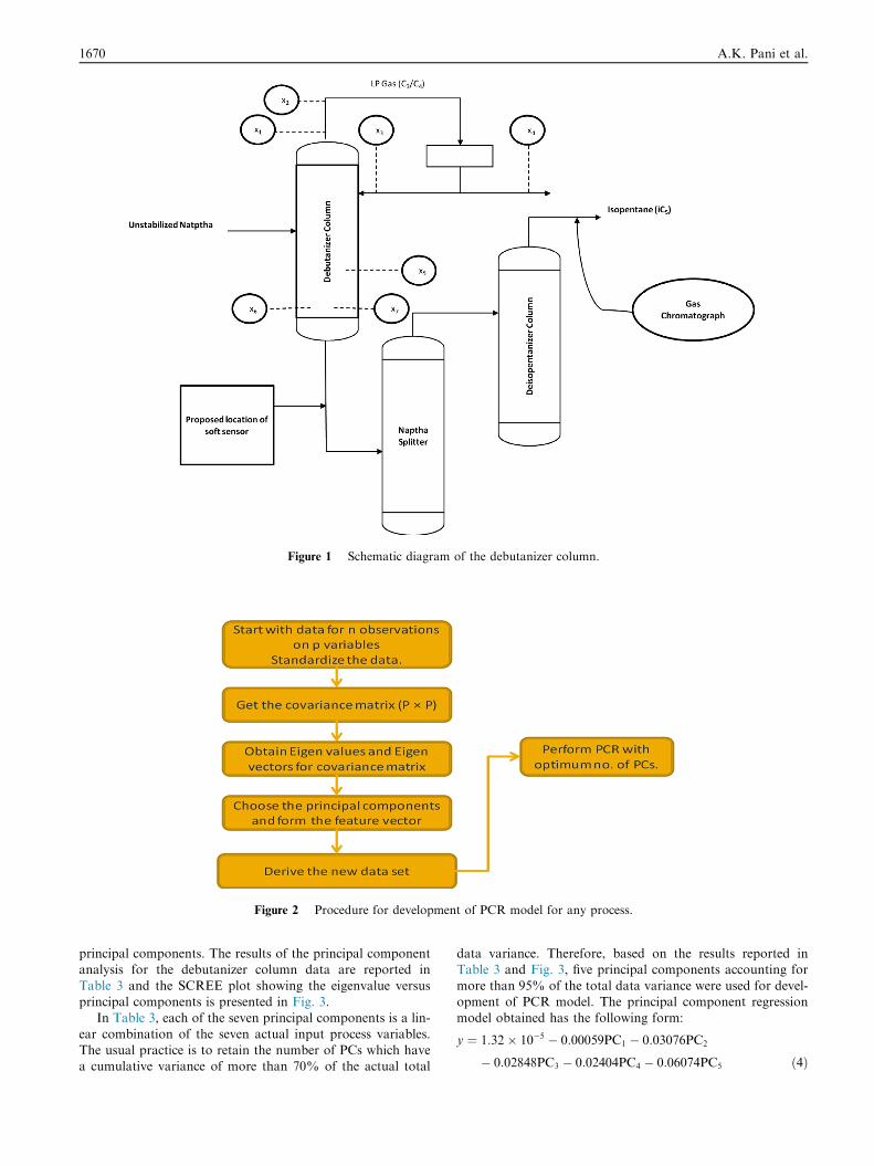
Figure 1 Schematic diagram of the debutanizer column.

Figure 2 Procedure for development of PCR model for any process.

1670 A.K. Pani et al.

principal components. The results of the principal componentanalysis for the debutanizer column data are reported in

Table 3 and the SCREE plot showing the eigenvalue versusprincipal components is presented in Fig. 3.

In Table 3, each of the seven principal components is a lin-

ear combination of the seven actual input process variables.The usual practice is to retain the number of PCs which havea cumulative variance of more than 70% of the actual total

data variance. Therefore, based on the results reported inTable 3 and Fig. 3, five principal components accounting for

more than 95% of the total data variance were used for devel-opment of PCR model. The principal component regressionmodel obtained has the following form:

y ¼ 1:32� 10�5 � 0:00059PC1 � 0:03076PC2

� 0:02848PC3 � 0:02404PC4 � 0:06074PC5 ð4Þ

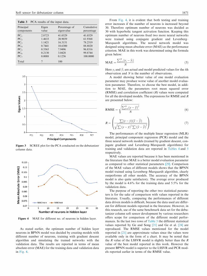
Table 3 PCA results of the input data.

Principal

components

Eigen

value

Percentage of

eigenvalue

Cumulative

percentage

PC1 2.8723 41.0329 41.0329

PC2 1.4633 20.9039 61.9368

PC3 1.1421 16.3151 78.2519

PC4 0.7441 10.6300 88.8820

PC5 0.5565 7.9496 96.8316

PC6 0.2130 3.0428 99.8744

PC7 0.0088 0.1256 100.0000

Total 7 100

Figure 3 SCREE plot for the PCA conducted on the debutanizer

column data.

Figure 4 MAE for different no. of neurons in hidden layer.

Soft sensor for debutanizer column 1671

As stated earlier, the optimum number of hidden layerneurons in BPNN model was decided by creating models with

different number of neurons, training with gradient descentalgorithm and simulating the trained networks with thevalidation data. The results are reported in terms of mean

absolute error (MAE) for the training data and validation datain Fig. 4.

From Fig. 4, it is evident that both testing and trainingerror increases if the number of neurons is increased beyond30. Therefore optimum number of neurons was decided as

30 with hyperbolic tangent activation function. Keeping thisoptimum number of neurons fixed two more neural networkswere trained using conjugate gradient and Levenberg–

Marquardt algorithms. The neural network model wasdesigned using mean absolute error (MAE) as the performancecriterion. MAE in this work was determined using the formula

given below:

MAE ¼PN

i¼1 yi � byij jN

ð5Þ

Here yi and byi are actual and model predicted values for the ith

observation and N is the number of observations.A model showing better value of one model evaluation

parameter may produce worse value of another model evalua-

tion parameter. Therefore, to choose the best model, in addi-tion to MAE, the parameters root mean squared error(RMSE) and correlation coefficient (R) values were computed

for all the developed models. The expressions for RMSE and Rare presented below:

RMSE ¼ffiffiffiffiffiffiffiffiffiffiffiffiffiffiffiffiffiffiffiffiffiffiffiffiffiffiffiPN

i¼1ðy� byÞ2N

sð6Þ

R ¼Pðy� �yÞðby � �byÞffiffiffiffiffiffiffiffiffiffiffiffiffiffiffiffiffiffiffiffiffiffiffiffiffiffiffiffiffiffiffiffiffiffiffiffiffiffiffiffiffiffiffiffiffiffiP ðy� �yÞ2 P ðby � �byÞ2q

0B@1CA ð7Þ

The performances of the multiple linear regression (MLR)model, principal component regression (PCR) model and thethree neural network models (trained by gradient descent, con-

jugate gradient and Levenberg–Marquardt algorithms) fortraining and validation data are reported in Tables 4 and 5respectively.

MAE values are reported because it has been mentioned inthe literature that MAE is a better model evaluation parameteras compared to other statistical parameters [29]. Comparisonof the MAE values of different models shows that the BPNN

model trained using Levenberg–Marquardt algorithm, clearlyoutperforms all other models. The accuracy of the BPNNmodel is also quite satisfactory. The average error produced

by the model is 4.6% for the training data and 5.5% for thevalidation data.

The purpose of reporting the other two statistical parame-

ters is for the sake of comparison with values reported in theliterature. Usually, comparing the performances of differentdata driven models is difficult, because the data used are differ-ent for different models reported in the literature. However, in

this research, use of the same benchmark data set for the debu-tanizer column soft sensor development by various researchersoffers scope for comparison of the different model perfor-

mances. In the last two rows of Table 5 the different statisticalvalues reported by Ge and Song [21] and Ge et al. [24] arereproduced. The RMSE values mentioned for the model

reported in [21] are approximate values since the values wereavailable only in the form of a chart. It may be noted thatthe R value of the LSSVR model is slightly better than the R

value of the best model reported in this work. However thepresent BPNN model is superior to the LSSVR and PCR mod-els reported earlier in terms of the RMSE value.

Table 4 Debutanizer column model performance for training data.

Model type Statistical model evaluation parameter

Mean absolute error

(MAE)

Root mean squared error

(RMSE)

Correlation

coefficient (R)

Multiple linear regression (MLR) 0.994 1.007 0.313

Principal component regression (PCR) 0.171 0.24 0.015

Back propagation neural network (BPNN)

trained by

Gradient-descent 0.094 0.144 0.537

Conjugate-

gradient

0.066 0.112 0.757

Levenberg–

Marquardt

0.046 0.064 0.925

Table 5 Debutanizer column model performance for validation data.

Model type Statistical model evaluation parameter

Mean absolute

error (MAE)

Root mean

squared error

(RMSE)

Correlation

coefficient

(R)

Models reported

in this work

Multiple linear regression (MLR) 0.989 0.999 0.395

Principal component

regression (PCR)

0.105 0.1511 0.148

Back propagation neural

network (BPNN) trained by

Gradient-descent 0.081 0.125 0.553

Conjugate-gradient 0.069 0.111 0.664

Levenberg–Marquardt 0.055 0.076 0.856

Models reported by

Ge and Song [21]

LSSVR Not reported 0.1418 0.9132

SVR Not reported 0.145 0.6897

PLS Not reported 0.165 0.4035

Model reported by

Ge et al. [24]

Non-linear semi supervised PCR Not reported 0.1499 Not reported

Figure 5 Prediction of C4 content in the debutanizer bottom product (training data).

1672 A.K. Pani et al.

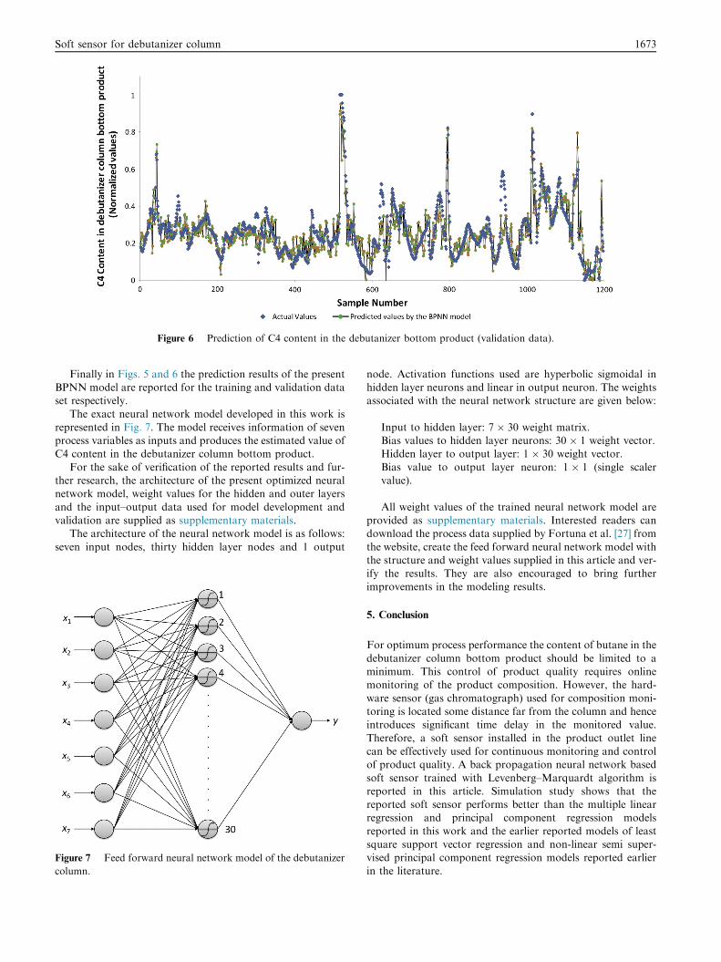
Figure 6 Prediction of C4 content in the debutanizer bottom product (validation data).

Soft sensor for debutanizer column 1673

Finally in Figs. 5 and 6 the prediction results of the presentBPNN model are reported for the training and validation dataset respectively.

The exact neural network model developed in this work is

represented in Fig. 7. The model receives information of sevenprocess variables as inputs and produces the estimated value ofC4 content in the debutanizer column bottom product.

For the sake of verification of the reported results and fur-ther research, the architecture of the present optimized neuralnetwork model, weight values for the hidden and outer layers

and the input–output data used for model development andvalidation are supplied as supplementary materials.

The architecture of the neural network model is as follows:

seven input nodes, thirty hidden layer nodes and 1 output

Figure 7 Feed forward neural network model of the debutanizer

column.

node. Activation functions used are hyperbolic sigmoidal inhidden layer neurons and linear in output neuron. The weightsassociated with the neural network structure are given below:

Input to hidden layer: 7 � 30 weight matrix.Bias values to hidden layer neurons: 30 � 1 weight vector.Hidden layer to output layer: 1 � 30 weight vector.

Bias value to output layer neuron: 1 � 1 (single scalervalue).

All weight values of the trained neural network model areprovided as supplementary materials. Interested readers candownload the process data supplied by Fortuna et al. [27] from

the website, create the feed forward neural network model withthe structure and weight values supplied in this article and ver-ify the results. They are also encouraged to bring furtherimprovements in the modeling results.

5. Conclusion

For optimum process performance the content of butane in the

debutanizer column bottom product should be limited to aminimum. This control of product quality requires onlinemonitoring of the product composition. However, the hard-

ware sensor (gas chromatograph) used for composition moni-toring is located some distance far from the column and henceintroduces significant time delay in the monitored value.

Therefore, a soft sensor installed in the product outlet linecan be effectively used for continuous monitoring and controlof product quality. A back propagation neural network based

soft sensor trained with Levenberg–Marquardt algorithm isreported in this article. Simulation study shows that thereported soft sensor performs better than the multiple linearregression and principal component regression models

reported in this work and the earlier reported models of leastsquare support vector regression and non-linear semi super-vised principal component regression models reported earlier

in the literature.

1674 A.K. Pani et al.

Appendix A. Supplementary material

Supplementary data associated with this article can be found,in the online version, at http://dx.doi.org/10.1016/j.aej.2016.

02.016.

References

[1] J. Shi, X.G. Liu, Product quality prediction by a neural soft-

sensor based on MSA and PCA, Int. J. Autom. Comput. 3

(2006) 17–22.

[2] H. Kaneko, K. Funatsu, Nonlinear regression method with

variable region selection and application to soft sensors,

Chemomet. Intell. Lab. Syst. 121 (2013) 26–32.

[3] P. Bogaerts, A.V. Wouwer, Software sensors for bioprocesses,

ISA Trans. 42 (2003) 547–558.

[4] M.H. Srour, V.G. Gomes, I.S. Altarawneh, J.A. Romagnoli,

Online model-based control of an emulsion terpolymerisation

process, Chem. Eng. Sci. 64 (2009) 2076–2087.

[5] O.A. Sotomayor, S.W. Park, C. Garcia, Software sensor for on-

line estimation of the microbial activity in activated sludge

systems, ISA Trans. 41 (2002) 127–143.

[6] A. Casali, G. Gonzalez, F. Torres, G. Vallebuona, L. Castelli, P.

Gimenez, Particle size distribution soft-sensor for a grinding

circuit, Powder Technol. 99 (1998) 15–21.

[7] Y.D. Ko, H. Shang, A neural network-based soft sensor for

particle size distribution using image analysis, Powder Technol.

212 (2011) 359–366.

[8] A.K. Pani, H.K. Mohanta, Soft sensing of particle size in a

grinding process: application of support vector regression, fuzzy

inference and adaptive neuro fuzzy inference techniques for

online monitoring of cement fineness, Powder Technol. 264

(2014) 484–497.

[9] B. Lin, B. Recke, J.K. Knudsen, S.B. Jørgensen, A systematic

approach for soft sensor development, Comput. Chem. Eng. 31

(2007) 419–425.

[10] A.K. Pani, V.K. Vadlamudi, H.K. Mohanta, Development and

comparison of neural network based soft sensors for online

estimation of cement clinker quality, ISA Trans. 52 (2013) 19–

29.

[11] J.V. Kresta, T.E. Marlin, J.F. MacGregor, Development of

inferential process models using PLS, Comput. Chem. Eng. 18

(1994) 597–611.

[12] F.Z. Chen, X.Z. Wang, Software sensor design using Bayesian

automatic classification and back-propagation neural networks,

Ind. Eng. Chem. Res. 37 (1998) 3985–3991.

[13] S. Park, C. Han, A nonlinear soft sensor based on multivariate

smoothing procedure for quality estimation in distillation

columns, Comput. Chem. Eng. 24 (2000) 871–877.

[14] S. Bhartiya, J.R. Whiteley, Development of inferential measure-

ments using neural networks, ISA Trans. 40 (2001) 307–323.

[15] L. Fortuna, A. Rizzo, M. Sinatra, M.G. Xibilia, Soft analyzers

for a sulfur recovery unit, Contr. Eng. Pract. 11 (2003) 1491–1500.

[16] W. Yan, H. Shao, X. Wang, Soft sensing modeling based on

support vector machine and Bayesian model selection, Comput.

Chem. Eng. 28 (2004) 1489–1498.

[17] M. Dam, D.N. Saraf, Design of neural networks using genetic

algorithm for on-line property estimation of crude fractionator

products, Comput. Chem. Eng. 30 (2006) 722–729.

[18] X. Yan, Modified nonlinear generalized ridge regression and its

application to develop naphtha cut point soft sensor, Comput.

Chem. Eng. 32 (2008) 608–621.

[19] H. Kaneko, M. Arakawa, K. Funatsu, Development of a new

soft sensor method using independent component analysis and

partial least squares, AIChE J. 55 (2009) 87–98.

[20] D. Wang, J. Liu, R. Srinivasan, Data-driven soft sensor

approach for quality prediction in a refining process, IEEE

Trans. Ind. Inf. 6 (2010) 11–17.

[21] Z. Ge, Z. Song, A comparative study of just-in-time-learning

based methods for online soft sensor modeling, Chemomet.

Intell. Lab. Syst. 104 (2010) 306–317.

[22] L. Fortuna, S. Graziani, M.G. Xibilia, Soft sensors for product

quality monitoring in debutanizer distillation columns, Contr.

Eng. Pract. 13 (2005) 499–508.

[23] Z. Ge, B. Huang, Z. Song, Mixture semisupervised principal

component regression model and soft sensor application,

AIChE J. 60 (2) (2014) 533–545.

[24] Z. Ge, B. Huang, Z. Song, Nonlinear semisupervised principal

component regression for soft sensor modeling and its mixture

form, J. Chemom. 28 (2014) 793–804.

[25] N.M. Ramli, M.A. Hussain, B.M. Jan, B. Abdullah,

Composition prediction of a debutanizer column using

equation based artificial neural network model,

Neurocomputing 131 (2014) 59–76.

[26] A.K. Pani, H.K. Mohanta, Online monitoring and control of

particle size in the grinding process using least square support

vector regression and resilient back propagation neural network,

ISA Trans. 56 (2015) 206–221.

[27] L. Fortuna, S. Graziani, A. Rizzo, M.G. Xibilia, Soft Sensors

for Monitoring and Control of Industrial Processes, Springer

Science & Business Media, 2007.

[28] M. Daszykowski, S. Serneels, K. Kaczmarek, P. Van Espen, C.

Croux, B. Walczak, TOMCAT: a MATLAB toolbox for

multivariate calibration techniques, Chemomet. Intell. Lab.

Syst. 85 (2007) 269–277.

[29] C. Willmott, K. Matsuura, Advantages of the mean absolute

error (MAE) over the root mean square error (RMSE) in

assessing average model performance, Clim. Res. 30 (2005) 79–

82.