real-time quality monitoring in debutanizer column with
TRANSCRIPT

ORIGINAL RESEARCH
Real-time quality monitoring in debutanizer column with regressiontree and ANFIS
Kumar Siddharth1 • Amey Pathak1 • Ajaya Kumar Pani1
Received: 8 August 2017 / Accepted: 22 May 2018� The Author(s) 2018
AbstractA debutanizer column is an integral part of any petroleum refinery. Online composition monitoring of debutanizer column
outlet streams is highly desirable in order to maximize the production of liquefied petroleum gas. In this article, data-driven
models for debutanizer column are developed for real-time composition monitoring. The dataset used has seven process
variables as inputs and the output is the butane concentration in the debutanizer column bottom product. The input–output
dataset is divided equally into a training (calibration) set and a validation (testing) set. The training set data were used to
develop fuzzy inference, adaptive neuro fuzzy (ANFIS) and regression tree models for the debutanizer column. The
accuracy of the developed models were evaluated by simulation of the models with the validation dataset. It is observed
that the ANFIS model has better estimation accuracy than other models developed in this work and many data-driven
models proposed so far in the literature for the debutanizer column.
Keywords Debutanizer column � ANFIS � Regression tree � Soft sensor
Introduction
Today, in a wide array of processes, it is difficult to achieve
continuous online monitoring. The prime reason is the low
reliability or unavailability of hardware sensors. This
results in huge revenue loss to the industry due to low-
quality products which could have been otherwise pre-
vented in presence of continuous monitoring. In order to
counter this problem, various industries are now incorpo-
rating soft sensor models to achieve quality monitoring.
There is increasing use of soft sensors in process industries
such as petroleum refinery (Wang et al. 2013; Shokri et al.
2015), cement (Pani and Mohanta 2014, 2016), polymer
(Shi and Liu 2006; Ahmed et al. 2009; Chen et al. 2013;
Sharma et al. 2017), metallurgy (Gui et al. 2005; Zhang
et al. 2013; Markopoulos et al. 2016), bioprocesses
(Steinwandter et al. 2016) and plasma etching process
(Zakour and Taleb 2017).
A debutanizer column is used to remove the lighter
fractions from gases, which are the overhead distillate
coming from the distillation unit. The debutanizer column
lacks real-time monitoring system for the butane (C4)
composition. Adding to the nonlinearity of the process, the
control of product quality tends to become a tricky issue in
the refinery. For the prediction of the bottom product
composition of the debutanizer column, various models
have been reported in the past. Significant among them are
backpropagation neural network (Fortuna et al. 2005; Pani
et al. 2016), partial least square (PLS; Ge and Song 2010;
Zheng et al. 2016), support vector regression (SVR; Ge and
Song 2010), principal component regression (PCR; Ge
et al. 2014), supervised latent factor analysis (Ge 2016;
Yao and Ge 2017), probabilistic regression (Yuan et al.
2015) and state-dependent ARX (Bidar et al. 2017) tech-
niques for modeling of debutanizer column.
Literature survey on modeling of debutanizer column
reveals that various types of PCR, PLS, probabilistic
regression, ARX and backpropagation neural network
models are reported. However, so far, the techniques of
fuzzy inference modeling and regression tree-based mod-
eling techniques have not been investigated for the debu-
tanizer column. Therefore, in this work, the performances
& Ajaya Kumar Pani
1 Department of Chemical Engineering, Birla Institute of
Technology and Science, Pilani 333031, India
123
Journal of Industrial Engineering Internationalhttps://doi.org/10.1007/s40092-018-0276-4(0123456789().,-volV)(0123456789().,-volV)

of fuzzy inference, adaptive neuro fuzzy (ANFIS) and
regression tree models are reported for the debutanizer
column. The required input output data are obtained from
the World Wide Web shared by Fortuna et al. (2007). The
data were statistically divided into a training set and a
validation set using Kennard–Stone algorithm (Kennard
and Stone 1969). The training set was used to develop
Mamdani and Sugeno-type fuzzy inference model, adap-
tive neuro fuzzy inference model and regression tree
models. All developed models are examined with unknown
data (validation set data) to assess the estimation accuracy
of the models. The performances of the developed models
were analyzed and compared by computing various sta-
tistical model evaluation parameters such as mean absolute
error (MAE), root-mean-squared error (RMSE) and corre-
lation coefficient (R). It was found that the adaptive neuro
fuzzy model is able to estimate the butane content in the
bottom stream of the debutanizer column with good
accuracy. The accuracy of the ANFIS model reported here
is even better than many other data-driven models pro-
posed so far in the literature.
The main contribution of this research is proposing a
model (with good accuracy of prediction) for the LPG
recovery unit of refinery. The use of the model will help to
overcome the problem of time delay arising due to the
hardware sensor. This will result in improved process
efficiency with maximization of LPG production. The rest
of the article is organized as follows. Process description
section contains the process description for the debutanizer
column and the scope of inferential model application in
the process. Details of the modeling techniques applied in
this research are presented in Methodology section fol-
lowed by results and discussion in Results and discussion
section. Finally, concluding remarks are presented in
Conclusion section.
Process description
A debutanizer column is present in various processing units
of a refinery. The column is used to remove the lighter
fractions from gasoline in the production of LPG and
gasoline. For instance, it is a part of the atmospheric and
vacuum crude distillation unit, cracking and coking units.
Unstabilized naphtha is fed to the debutanizer column. The
products coming out from the column are LPG as the top
product and gasoline/stabilized naphtha as the bottom
product. A simplified schematic flowsheet of the debu-
tanization process is shown in Fig. 1. The detailed process
flowsheet can be referred to in Fortuna et al. (2005).
Scope of the present research work
The butane (C4) content in the bottom product needs to be
minimized for better performance of the process (maximiz-
ing LPG in the top product). This requires continuous
monitoring of C4 content in the bottom product. A gas
chromatograph is used in the process to achieve this. But this
hardware sensor is located in the overhead of the deisopen-
tanizer column rather than being in the bottom flow line
coming from the debutanizer column. This results in a time
delay of 30–75 min in the composition measurement (For-
tuna et al. 2005). Therefore, to overcome this problem of
time delay, an inferential process model can be incorporated
in the bottom flow of debutanizer column to achieve real-
time monitoring of C4 content from the knowledge of other
process inputs. The various process inputs influencing theC4
content in the bottom stream are listed in Table 1. The output
to be predicted by the soft sensor model is the C4 content
present in the debutanizer column bottom product.
Methodology
The required process input–output data were obtained from
the internet resource mentioned in (Fortuna et al. 2007). This
has a total of 2394 observations (samples). This dataset was
split equally into a training set consisting of 1197 samples and
a validation set of the same dimension. The training set was
used formodel development, and the validation set wasmeant
for subsequent model performance assessment. The splitting
was done so as to ensure that the training set becomes a proper
representative of the entire set. The widely used distance-
based statistical technique, the Kennard–Stone algorithm
(Kennard and Stone 1969), was used for data division. The
followingmodeling techniques were followed in this research
for modeling of the debutanizer column.
Classification and regression tree (CART) modeldevelopment
CART method involves the progressive binary splits of
various estimations of classification variable to generate a
decision tree. Every estimation of every indicator variable
is taken into account as a potential split and the ideal split
is chosen in view of impurity criterion. A set of explana-
tory variables or predictors are used to study the variation
of the new data. Recursive binary splits are made on the
data creating mutually exclusive subgroups containing
objects with similar properties. An extremely intriguing
preferred standpoint of CART is the likelihood to manage
vast quantities of both categorical and numerical factors.
Another favorable position is that no assumption about the
Journal of Industrial Engineering International
123

hidden circulation of the predictor factors is required (even
categorical variables can be utilized). Eventually, CART
gives a graphical representation, which makes the under-
standing of the outcomes simple. Five elements are nec-
essary to develop a classification tree (Breiman et al.
1984): (1) a set of binary questions, (2) a measure to
optimize the split, (3) a stop-splitting rule, (4) a rule for
assigning termination code classification and (5) a method
to prune the tree back. The structure of a typical CART
model is shown in Fig. 2 (Breiman et al. 1984).
The tree growing procedure in CART is roughly anal-
ogous to a stepwise linear regression procedure which
consists of the following steps: (1) defining an initial set of
variables, (2) choosing the fitting method of least squares,
(3) defining the threshold P values for new variables to be
entered or removed from the equation, (4) backward
elimination of variables and selection of the best multi-
variable model based on the adjusted R2 values.
The designed training set was used to build up the
CART model for the debutanizer model. The resulting
model is shown in Fig. 3.
However, because of the large dimension data set (1197
objects), the initial CART model is highly complex with a
very high number of nodes. This model produces very
accurate prediction for the training data but largely fails to
predict accurately when supplied with unknown data (the
objects of validation set). This is the well-known overfit-
ting problem. The determination of a smaller tree, got from
the maximal one, is therefore essential for successful
modeling. The choice of the ideal tree is accomplished by a
tree pruning methodology. Many techniques were used to
generate the optimal model like examination of resubsti-
tution error, cross-validation, control depth, evaluating
root-mean-squared error (RMSE), correlation coefficient
(R) and mean absolute error (MAE).
Resubstitution error is difference between the predic-
tions of the model and that of the response training data.
High resubstitution error signifies lower accuracy in pre-
dictions. However, great predictions for new data aren’t
assured by having low resubstitution error.
Tree was cross-validated to see how accurate it could
predict for the new data; training data were split into 10
parts at random. On 9 parents of the data, 10 new trees
were trained. Predictive accuracy for each newly developed
tree was examined on the data which was not there in the
training. The technique gives a decent gauge on how
accurate is developed model.
A leafy tree with depth (many nodes) is generally very
precise on the training data. However, the model is not
ensured to demonstrate a tantamount exactness on a test
set. A deep tree’s test accuracy is frequently far not as
much as its training (resubstitution) accuracy as it tends to
Fig. 1 Schematic process
diagram of the debutanizer
column
Table 1 Input and output variables for the proposed inferential
model of the debutanizer column
Variables Description
Inputs
x1 Top tray temperature
x2 Top pressure
x3 Reflux flow
x4 Flow to next process
x5 Sixth tray temperature
x6 Bottom tray temperature 1
x7 Bottom tray temperature 2
Output
y Butane (C4) content in the debutanizer column bottom
Journal of Industrial Engineering International
123

overtrain (or overfit). Conversely, a shallow tree does not
achieve high training precision.
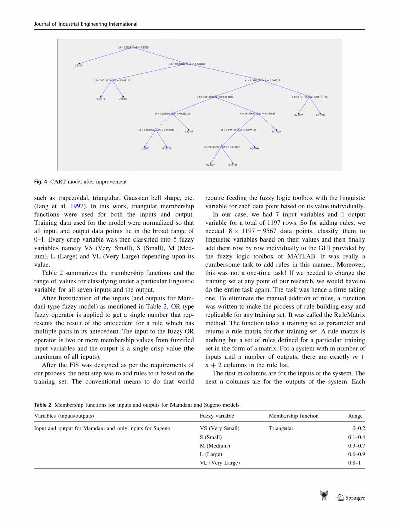
The regression tree model after improvement is pre-
sented in Fig. 4.
Mamdani and Sugeno fuzzy inference modeldevelopment
The entire activity of fuzzy inference model designing is a
sequence of five steps: fuzzification of the input (predictor)
process variables, application of the appropriate AND or
OR operator in the antecedent, implication from the ante-
cedent to the consequent by application of the fuzzy if then
rule, aggregation of the consequents across the rules to get
the output (response) process variable in fuzzified form and
finally defuzzification of the fuzzified output (Jang et al.
1997; Pani and Mohanta 2014).
In the fuzzification step, membership functions were
decided to create valid fuzzy sets to accommodate all
inputs. The membership functions can take many forms
Fig. 2 A typical CART model
Fig. 3 Initial CART model of the debutanizer column
Journal of Industrial Engineering International
123
such as trapezoidal, triangular, Gaussian bell shape, etc.
(Jang et al. 1997). In this work, triangular membership
functions were used for both the inputs and output.
Training data used for the model were normalized so that
all input and output data points lie in the broad range of
0–1. Every crisp variable was then classified into 5 fuzzy
variables namely VS (Very Small), S (Small), M (Med-
ium), L (Large) and VL (Very Large) depending upon its
value.
Table 2 summarizes the membership functions and the
range of values for classifying under a particular linguistic
variable for all seven inputs and the output.
After fuzzification of the inputs (and outputs for Mam-
dani-type fuzzy model) as mentioned in Table 2, OR type
fuzzy operator is applied to get a single number that rep-
resents the result of the antecedent for a rule which has
multiple parts in its antecedent. The input to the fuzzy OR
operator is two or more membership values from fuzzified
input variables and the output is a single crisp value (the
maximum of all inputs).
After the FIS was designed as per the requirements of
our process, the next step was to add rules to it based on the
training set. The conventional means to do that would
require feeding the fuzzy logic toolbox with the linguistic
variable for each data point based on its value individually.
In our case, we had 7 input variables and 1 output
variable for a total of 1197 rows. So for adding rules, we
needed 8 9 1197 = 9567 data points, classify them to
linguistic variables based on their values and then finally
add them row by row individually to the GUI provided by
the fuzzy logic toolbox of MATLAB. It was really a
cumbersome task to add rules in this manner. Moreover,
this was not a one-time task! If we needed to change the
training set at any point of our research, we would have to
do the entire task again. The task was hence a time taking
one. To eliminate the manual addition of rules, a function
was written to make the process of rule building easy and
replicable for any training set. It was called the RuleMatrix
method. The function takes a training set as parameter and
returns a rule matrix for that training set. A rule matrix is
nothing but a set of rules defined for a particular training
set in the form of a matrix. For a system with m number of
inputs and n number of outputs, there are exactly m ?
n ? 2 columns in the rule list.
The first m columns are for the inputs of the system. The
next n columns are for the outputs of the system. Each
Fig. 4 CART model after improvement
Table 2 Membership functions for inputs and outputs for Mamdani and Sugeno models
Variables (inputs/outputs) Fuzzy variable Membership function Range
Input and output for Mamdani and only inputs for Sugeno VS (Very Small) Triangular 0–0.2
S (Small) 0.1–0.4
M (Medium) 0.3–0.7
L (Large) 0.6–0.9
VL (Very Large) 0.8–1
Journal of Industrial Engineering International
123

column contains a number that refers to the index of the
membership function for that variable. The m ? n ? 1
column contains the weight applied to each rule. As
specified earlier, it is 1 for each rule in our case. The
m ? n ? 2 column contains a 1 if the fuzzy operator for
the rule’s antecedent is AND. It contains a 2 if the fuzzy
operator is OR. AND was used as the fuzzy operator in our
case for the rules.
The rule matrix was then added to the FIS through a
single line of code. This has made the entire process easy,
reproducible and adaptable for different training sets by
just changing one line in the entire code.
For development of Sugeno-type fuzzy model, the prime
difference is in the definition of membership values for
output variable which was defined to constant values in the
range 0–1 (zero-order Sugeno fuzzy model). The mam2sug
MATLAB function method takes a Mamdani-type FIS as
parameter and returns a corresponding zero-order Sugeno-
type FIS for the process. The resulting Sugeno-type FIS has
output membership functions with values corresponding to
the centroids of that in Mamdani-type FIS passed as
parameter. It uses weighted-average defuzzification
method and the product implication method. All the other
properties like the input membership functions and the rule
definitions of the resulting FIS are identical to the Mam-
dani-type FIS passed to it.
Adaptive neuro fuzzy inference (ANFIS) modeldevelopment
This technique was first proposed by Jang (1993) and has
subsequently become one of the most popular hybrid
modeling techniques combining neural network and fuzzy
inference concepts. ANFIS takes a Sugeno-type FIS as
input and then trains its membership function parameters.
The initial fuzzy model is required to determine the num-
ber of inputs, linguistic variable and the number of rules in
the tuned final model. The FIS must have the following
properties for the ANFIS to support it:-
1. Only zeroth- and first-order Sugeno-type FIS.
2. Output membership functions uniformly of the same
type, i.e., linear or constant. The FIS must have a
single output.
3. Number of output membership function must be equal
to the number of rules, i.e., no two rules can share the
same output membership function.
4. Have the same weight for each rule, i.e., 1.
The Sugeno-type FIS designed earlier will not be sup-
ported by the ANFIS. It is because the FIS had 350 rules
while the number of output membership functions was 5.
This clearly hints at rule sharing which is not supported by
the ANFIS.
Hence a new FIS had to be designed such that it com-
plies with all the requirements for it to be supported by the
ANFIS. The number of rules can be reduced and fine-tuned
by using various clustering methods on the training data.
Clustering methods analyze the intrinsic grouping in a
dataset. The two most widely used methods are grid par-
titioning and subtractive clustering.
In grid partitioning technique, the antecedents of the
fuzzy rules are formed by partitioning the input space into
numerous fuzzy regions. It is a rather subjective approach
because the user has to initially specify the number of
clusters in which the variables will be partitioned into. The
product of number of clusters for each input variables then
gives the total number of rules.
The grid partitioning method leads to a problem when
the number of inputs is large. The method requires enu-
merating all possible combinations of input membership
functions to generate rules, and hence, the number of rules
blows up in the case of more inputs. In our case of 7 inputs,
each with say 5 membership functions, this method will
lead to 78,125(= 55) rules. Hence, the number of rules
grows exponentially with the increase in number of inputs.
Such systems then are infeasible for any training. This
exponential blowing up of number of rules with the
increase in number of inputs is often referred to as the
‘curse of dimensionality.’
So keeping in mind the above constraint, the number of
membership function for the 7 inputs of the debutanizer
column was kept as low as 2. That led to 128 (= 27) rules
and could be further trained using ANFIS. The membership
functions were marked S and L denoting ‘small’ and
‘large,’ respectively. The model was chosen to be a zeroth-
order Sugeno model. The membership functions were
chosen to be of the triangular type.
The above fuzzy model obtained by grid partitioning
was trained by updating the consequent parameters of the
rules by least square estimation algorithm and the premise
parameters by the backpropagation gradient descent algo-
rithm. This is also known as the hybrid learning algorithm.
The curse of dimensionality renders the grid partitioning
method impractical for large number of inputs. For
instance, if the above fuzzy model was attempted with 3
membership functions for each input, the number of rules
would have exceeded 2000. Therefore, the number of
membership functions was restricted in the case of grid
partitioning algorithm.
A much more intuitive technique is the subtractive
clustering algorithm. Subtractive clustering is a one pass
algorithm that estimates the number of clusters and the
cluster centers for the input–output pair in the data set. It
works by determining regions of high densities in the data
space. A point is chosen to be the cluster center if it has
maximum no. of neighbors. User specifies a fuzzy radius
Journal of Industrial Engineering International
123
till which the points are left out, and the algorithm tries to
find the next cluster center in the remaining points. In this
manner, all the data points are examined.
This algorithm does not lead to the dimensionality issue.
Number of rules and antecedent membership functions are
first determined by the rule extraction method. Linear least
squares estimation is then used to determine the consequent
of each rule.
This algorithm requires the user to specify the radius of
influence of the cluster centers for each input. This values
lies between 0 and 1 considering the entire data set as a unit
hypercube. Also the accept ratio and the reject ratios needs
to be specified which instructs the algorithm to accept the
data points as cluster centers if their density potential lies
above the accept ratio and reject them if the potential lies
below the reject ratios.
For the final model generated using subtractive clus-
tering, the radii of influence were set to 0.22 for all inputs.
The accept ratio was set to be 0.6, and the reject ratio was
set to 0.1. This generates a Sugeno FIS with 54 member-
ship functions and 54 rules.
Results and discussion
The initial regression tree model was developed with the
leaf size of 1. Though it has good accuracy, the model is
extremely complex. As the leaf size was increased error
also increased, i.e., model became less accurate. For the
given data when Min leaf size vs cross-validated error
graph was generated, it was found out that the cross-vali-
dated error was least for the 77.5 min leaf size. The best
leaf size is 77.5 or 78. Therefore, leaf size of 78 was
decided to be somewhat optimum at which the model is
relatively much simpler and at the same time does not have
very high error value.
The resubstitution loss is the MSE (mean squared error)
of prediction. This was computed to be 0529.
The cross-validated loss was computed to be 0.0177,
which signifies a common predictive error of model to be
0.133. This signifies that simple resubstitution loss is typ-
ically lower than cross-validated loss.
The optimal regression tree generated gives very high
resubstitution error and is much smaller. Yet, it gives
comparable precision. Even though cross-validation error
was low for the generated model other errors [root-mean-
squared error (RMSE), correlation coefficient (R), mean
absolute error (MAE)] were really high as compared to the
original model.
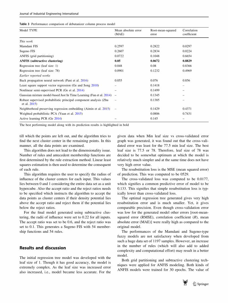
The performances of the Mamdani and Sugeno-type
fuzzy models are not satisfactory when developed from
such a huge data set of 1197 samples. However, an increase
in the number of rules (which will also add to added
complexity and computational effort) may result in a better
model.
Both grid partitioning and subtractive clustering tech-
niques were applied for ANFIS modeling. Both kinds of
ANFIS models were trained for 30 epochs. The value of
Table 3 Performance comparison of debutanizer column process model
Model TYPE Mean absolute error
(MAE)
Root-mean-squared
error
Correlation
coefficient
This work
Mamdani FIS 0.2597 0.2822 0.0297
Sugeno FIS 0.2607 0.2834 0.0224
ANFIS (grid partitioning) 0.0722 0.1048 0.6654
ANFIS (subtractive clustering) 0.05 0.0672 0.8829
Regression tree (leaf size: 1) 0.048 0.08 0.8366
Regression tree (leaf size: 78) 0.0901 0.1232 0.4969
Earlier reported works
Back propagation neural network (Pani et al. 2016) 0.055 0.076 0.856
Least square support vector regression (Ge and Song 2010) – 0.1418 –
Nonlinear semi-supervised PCR (Ge et al. 2014) – 0.1499 –
Gaussian mixture model-based Just In Time Learning (Fan et al. 2014) – 0.1345 –
Robust supervised probabilistic principal component analysis (Zhu
et al. 2015)
– 0.1385 –
Neighborhood preserving regression embedding (Aimin et al. 2015) – 0.1429 0.4371
Weighted probabilistic PCA (Yuan et al. 2015) 0.0806 0.7431
Active learning PCR (Ge 2014) – 0.145 –
The best performing model along with its prediction results is highlighted in bold
Journal of Industrial Engineering International
123
error drops with each training epoch. The models trained
using the training set were validated by the test set. The
value of error goes down for the test set too with the
number of training epoch till it finally converges to a
constant value. The RMSE values converged at 0.109 and
0.105 for training set and the test set, respectively, for the
grid partition-based ANFIS model. For the subtractive
clustering based model, the RMSE values converged at
0.0539 and 0.0672 for training set and the test set,
respectively.
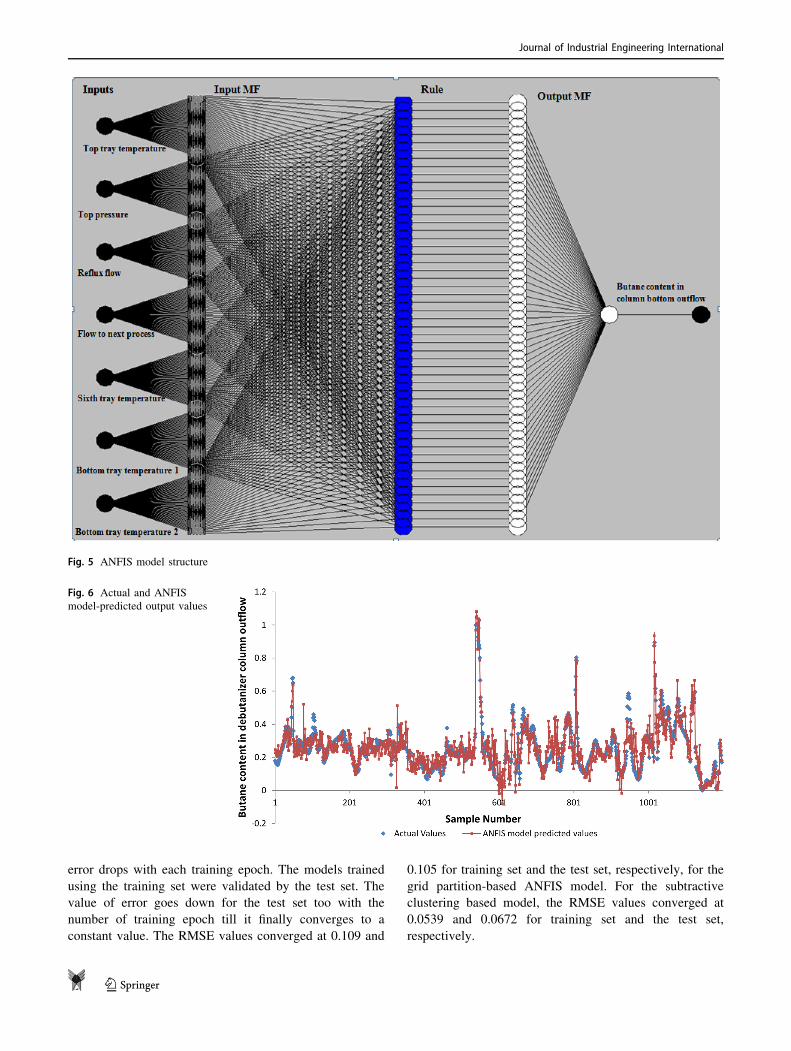
Fig. 5 ANFIS model structure
Fig. 6 Actual and ANFIS
model-predicted output values
Journal of Industrial Engineering International
123
The predicted values were compared with the actual
values in the data, and the values of MAE, RMSE and R
were computed for different models. The formulas used for
computation of various statistical parameters are men-
tioned below:
Mean absolute error is a quantity used to evaluate how
close the predictions are to the output. It is given by:
MAE ¼PN
i¼1yi�byij j
N.
Root-mean-squared error gives an index to analyze the
precision with which the model predicts the output. It is
given by: RMSE ¼
ffiffiffiffiffiffiffiffiffiffiffiffiffiffiffiffiffiffiffiffiffiffiffiPN
i¼1yi�byið Þ2N
r
where yi and byi are
actual and predicted values, respectively, N is the no. of
rows.
Correlation coefficient provides an index to measure the
linear dependence between two vectors X and Y. It gives a
value ranging from - 1 to ?1. The value 1 signifies total
positive linear correlation, 0 no linear correlation, whereas
- 1 signifies total negative linear correlation. For a sample,
the correlation coefficient is given by:
R ¼P
y� yð Þ by � by� �
ffiffiffiffiffiffiffiffiffiffiffiffiffiffiffiffiffiffiffiffiffiffiffiffiffiffiffiffiffiffiffiffiffiffiffiffiffiffiffiffiffiffiffiffiffiP
y� yð Þ2P
by � by� �2
r
0
BB@
1
CCA
yi byi are actual and predicted values, respectively, N is the
no. of rows.
The prediction performances of all models for the val-
idation data are presented in Table 3.
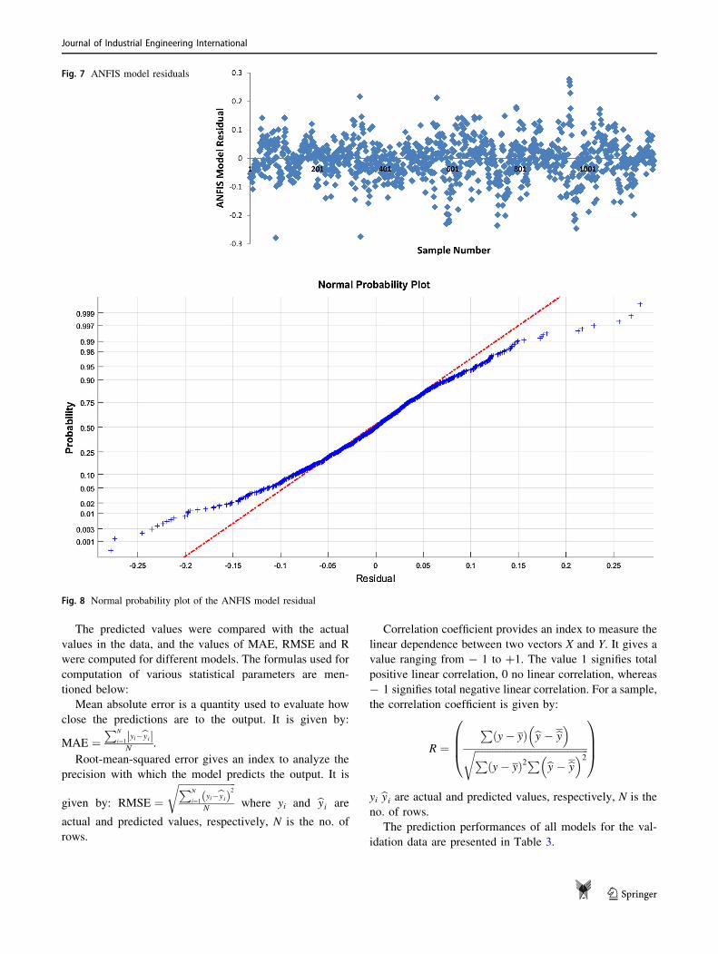
Fig. 7 ANFIS model residuals
Fig. 8 Normal probability plot of the ANFIS model residual
Journal of Industrial Engineering International
123

From Table 3, it is quite clear that the proposed adaptive
neuro fuzzy inference model designed using subtractive
clustering algorithm regression tree model, Mamdani and
Sugeno fuzzy inference models and a few other models
(neural network, just in time and principal component
regression) reported in the literature for the same process
and using the same benchmark dataset. The structure of the
proposed ANFIS model is shown in Fig. 5. The model has
7 inputs, 1 output and a total of 54 rules.
Error analysis of the proposed ANFIS model
The accuracy of the designed ANFIS model is further
tested by conducting rigorous error analysis between the
actual and model-predicted output values (i.e., butane
content in the debutanizer column bottom product stream).
It may be noted that all the error analysis is done by sim-
ulation of the model to unknown inputs (validation data).
The actual values and the predicted values by the ANFIS
model are shown in Fig. 6.
Table 3 and Fig. 6 indicate that the predicted output of
the ANFIS model is quite close to the actual output values.
However, the accuracy of the model is further tested by
conducting error analysis of model residuals. Two kinds of
error analysis are reported in this work which are presented
in Figs. 7 and 8.
In simulation of the model with the validation set input
data, Fig. 7 presents the plot of model residuals (i.e., dif-
ference between actual output and model-predicted output).
It is clear that the residuals are perfectly random in nature
without any particular trend w.r.t the sample number (or
time instances). Figure 8 shows the normal probability plot
of the prediction errors which indicates that most of the
errors’ probability values match satisfactorily with the
analytic line. Randomness and normal distribution of the
prediction errors are important requirements of a good
model (Ljung 1998). Table 3 and Figs. 6 to 8 indicate that
the ANFIS model simulation with unknown inputs results
in outputs whose error values are less, randomly distributed
and come from a normal distribution.
Conclusion
Data-driven models were developed in the present work for
real-time monitoring of butane (C4) content in the bottom
stream of debutanizer column. Mamdani and Sugeno-type
fuzzy inference models, regression tree-based model and
adaptive neuro fuzzy model were developed. All models
were analyzed by assessing their prediction performances
with unknown data. It was found that the neuro fuzzy
model reported in this work results in better performance
than other models developed in this work and developed in
earlier works reported in literature. The good performance
of the neuro fuzzy model makes it a suitable option for
being used for real-time monitoring in petroleum refineries.
Open Access This article is distributed under the terms of the Creative
Commons Attribution 4.0 International License (http://creative
commons.org/licenses/by/4.0/), which permits unrestricted use, dis-
tribution, and reproduction in any medium, provided you give
appropriate credit to the original author(s) and the source, provide a
link to the Creative Commons license, and indicate if changes were
made.
References
Ahmed F, Nazir S, Yeo YK (2009) A recursive PLS-based soft sensor
for prediction of the melt index during grade change operations
in HDPE plant. Korean J Chem Eng 26(1):14–20
Aimin M, Peng L, Lingjian Y (2015) Neighborhood preserving
regression embedding based data regression and its applications
on soft sensor modeling. Chemometr Intell Lab Syst 147:86–94
Bidar B, Sadeghi J, Shahraki F, Khalilipour MM (2017) Data-driven
soft sensor approach for online quality prediction using state
dependent parameter models. Chemometr Intell Lab Syst
162:130–141
Breiman L, Friedman J, Stone CJ, Olshen RA (1984) Classification
and regression trees. CRC Press, Hoboken
Chen WL, Huang CY, Huang CY (2013) Finding efficient frontier of
process parameters for plastic injection molding. J Ind Eng Int
9(1):25
Fan M, Ge Z, Song Z (2014) Adaptive Gaussian mixture model-based
relevant sample selection for JITL soft sensor development. Ind
Eng Chem Res 53(51):19979–19986
Fortuna L, Graziani S, Xibilia MG (2005) Soft sensors for product
quality monitoring in debutanizer distillation columns. Control
Eng Pract 13(4):499–508
Fortuna L, Graziani S, Rizzo A, Xibilia MG (2007) Soft sensors for
monitoring and control of industrial processes. Springer, Berlin
Ge Z (2014) Active learning strategy for smart soft sensor develop-
ment under a small number of labeled data samples. J Process
Control 24(9):1454–1461
Ge Z (2016) Supervised latent factor analysis for process data
regression modeling and soft sensor application. IEEE Trans
Control Syst Technol 24(3):1004–1011
Ge Z, Song Z (2010) A comparative study of just-in-time-learning
based methods for online soft sensor modeling. Chemometr
Intell Lab Syst 104(2):306–317
Ge Z, Huang B, Song Z (2014) Nonlinear semisupervised principal
component regression for soft sensor modeling and its mixture
form. J Chemom 28(11):793–804
Gui WH, Li YG, Wang YL (2005) Soft sensor for ratio of soda to
aluminate based on PCA-RBF multiple network. J Cent South
Univ Technol 12(1):88–92
Jang JS (1993) ANFIS: adaptive-network-based fuzzy inference
system. IEEE Trans Syst Man Cybern 23(3):665–685
Jang JSR, Sun CT, Mizutani E (1997) Neuro-fuzzy and soft
computing: a computational approach to learning and machine
intelligence. Prentice Hall, India
Kennard RW, Stone LA (1969) Computer aided design of experi-
ments. Technometrics 11(1):137–148
Ljung L (1999) System Identification: theory for the User, 2nd edn.
Englewood Cliffs, NJ, Prentice-Hall, USA
Journal of Industrial Engineering International
123

Markopoulos AP, Georgiopoulos S, Manolakos DE (2016) On the use
of back propagation and radial basis function neural networks in
surface roughness prediction. J Ind Eng Int 12(3):389–400
Pani AK, Mohanta HK (2014) Soft sensing of particle size in a
grinding process: application of support vector regression, fuzzy
inference and adaptive neuro fuzzy inference techniques for
online monitoring of cement fineness. Powder Technol
264:484–497
Pani AK, Mohanta HK (2016) Online monitoring of cement clinker
quality using multivariate statistics and Takagi–Sugeno fuzzy-
inference technique. Control Eng Pract 57:1–17
Pani AK, Amin KG, Mohanta HK (2016) Soft sensing of product
quality in the debutanizer column with principal component
analysis and feed-forward artificial neural network. Alex Eng J
55(2):1667–1674
Sharma GVSS, Rao RU, Rao PS (2017) A Taguchi approach on
optimal process control parameters for HDPE pipe extrusion
process. J Ind Eng Int 13(2):215–228
Shi J, Liu XG (2006) Product quality prediction by a neural soft-
sensor based on MSA and PCA. Int J Autom Comput 3(1):17–22
Shokri S, Sadeghi MT, Marvast MA, Narasimhan S (2015) Improve-
ment of the prediction performance of a soft sensor model based
on support vector regression for production of ultra-low sulfur
diesel. Pet Sci 12(1):177–188
Steinwandter V, Zahel T, Sagmeister P, Herwig C (2017) Propagation
of measurement accuracy to biomass soft-sensor estimation and
control quality. Anal bioanal chem 409:693–706
Wang Y, Chen C, Yan X (2013) Structure and weight optimization of
neural network based on CPA-MLR and its application in
naphtha dry point soft sensor. Neural Comput Appl 22(1):75–82
Yao L, Ge Z (2017) Locally weighted prediction methods for latent
factor analysis with supervised and semisupervised process data.
IEEE Trans Autom Sci Eng 14(1):126–138
Yuan X, Ye L, Bao L, Ge Z, Song Z (2015) Nonlinear feature
extraction for soft sensor modeling based on weighted proba-
bilistic PCA. Chemometr Intell Lab Syst 147:167–175
Zakour SB, Taleb H (2017) Endpoint in plasma etch process using
new modified w-multivariate charts and windowed regression.
J Ind Eng Int 13(3):307–322
Zhang Shuning, Wang Fuli, He Dakuo, Chu Fei (2013) Soft sensor for
cobalt oxalate synthesis process in cobalt hydrometallurgy based
on hybrid model. Neural Comput Appl 23(5):1465–1472
Zheng J, Song Z, Ge Z (2016) Probabilistic learning of partial least
squares regression model: theory and industrial applications.
Chemometr Intell Lab Syst 158:80–90
Zhu J, Ge Z, Song Z (2015) Robust supervised probabilistic principal
component analysis model for soft sensing of key process
variables. Chem Eng Sci 122:573–584
Journal of Industrial Engineering International
123