solutions for co2 capture from coal-fired power plants phd thesis.pdfcapture from coal-fired power...
TRANSCRIPT

UNIVERSITÀ DEGLI STUDI DI FIRENZE
FACOLTÀ DI INGEGNERIA
Tesi di dottorato
2009
Solutions for CO2 capture
from coal-fired power plants
Influence on plant performance
and environmental impact
Relatore: Prof. Ing. G.MANFRIDA
Co-relatore: Ing. D.FIASCHI
Contro-relatore: Prof. Ing. P. CONSONNI
Candidato:
Robert Strube


i
Acknowledgments
I am grateful to many people who helped me complete this Ph.D. thesis.
Above all, many thanks to Prof. G. Manfrida for his support and for giving me this research opportu-
nity in this interesting field of work that may help make power production from fossil fuels more en-
vironmentally friendly.
I also wish to thank G. Pellegrini for his support and friendship, and all the friends I had the chance to
meet in Florence for making me feel welcome in Italy.
The financial support by the European Commission in the context of the 6th Framework Programme
(INSPIRE; Marie Curie Research Training Network, MRTN-CT-2005-019296) is gratefully ac-
knowledged.
Thanks to Jorge M. Plaza from the Department of Chemical Engineering at the University of Texas at
Austin for his support with the absorber model for CO2 removal with monoethanolamine.
The discussion with Vincent White at Air Products, UK was of great help for understanding the rele-
vant practical problems involved with features of CO2 purification.
The opportunity to investigate CO2 purification for an oxy-fuel plant at IEA GHG in Cheltenham, UK
under the supervision of Stanley Santos as a secondment within the INSPIRE programme is greatly
appreciated.
I also want to thank the administrative staff at the Dipartimento di Energetica “Sergio Stecco” for
their support.
Finally, I want to thank my father W. Strube for his patience and the indispensable help with proof-
reading all my work.

ii
Introduction
Global warming caused by the emission of anthropogenic greenhouse gases, especially of CO2,
is nowadays one of the major environmental issues. However, there are a number of mitigation op-
tions that can help reduce the emission of greenhouse gases. These options comprise, for example,
reforestation and a change in agriculture. For the energy sector, some of these options are energy sav-
ings, increased power plant efficiency, e.g. by using co-generation of heat and electricity, the use of
renewables and switching to low-carbon fuels such as natural gas. It is clear that one of these choices
alone is not capable of sufficiently reducing greenhouse gas emissions. All possibilities for the reduc-
tion of greenhouse gas emissions have to be employed in order to at least significantly slow down
global warming.
In this thesis, the author concentrated on a relatively new mitigation option. Fossil fuels still are
- and in the short to medium term will remain - the main resource for energy production. Especially
coal is a fossil resource that is expected to be available for some hundred years or more. Therefore,
greenhouse gas emissions due to its use have to be reduced by some sort of CO2 elimination in the so-
called carbon capture and storage process (CCS).
In order to reduce CO2 emissions from a power plant, CO2 can either be captured from the flue
gases or from the syngas stream in a gasification plant. Although smaller pilot plants already exist to
study their performance, CCS needs to be applied to larger power plants of about or more than 500
MW output such as the ones studied in this thesis in order for this mitigation to be effective on a
global scale.
The author developed models with the flowsheet simulation program Aspen Plus to study the
most common power plant processes and their performance with and without capture. All models
were designed to achieve a nominal CO2 capture efficiency of 90%. In a first step, models were de-
veloped that assume chemical and vapour-liquid equilibrium. In order for the models to be as realistic
as possible, focus was then laid on rate-based models that take into account the kinetics of the occur-
ring chemical reactions and of mass transfer.
The rate-based models studied in this thesis are for
i) a 500 MW pulverized coal power plant using monoethanolamine (MEA) and ammonia
as chemical solvents for post-combustion CO2 capture,
ii) a 500 MW Internal Gasification Combined Cycle (IGCC) with pre-combustion capture,
using the physical solvent Selexol for either separate or co-capture of CO2 and H2S, and
iii) a 500 MW oxy-fuel power plant with cryogenic CO2 purification.
For all models, the author compares the effect of CO2 capture on power plant performance. In
accordance with literature, the largest energy penalty due to CO2 capture was caused by the necessary
thermal regeneration of chemical solvents used in post-combustion capture in this study.

iii
In order to determine the environmental impact of the investigated power plants, a consecutive
Life Cycle Assessment (LCA) was carried out with the commercial software SimaPro. The LCA con-
firmed the findings of the energy analysis.
The highest environmental impact per net energy output is observed for post-combustion cap-
ture. This impact was not only caused by the high energy penalty but also by the necessary solvent
production to compensate for solvent losses to the atmosphere and solvent degradation. The environ-
mental impact of the IGCC with pre-combustion capture was lower and of similar magnitude as for
the oxy-fuel power plant.
Finally an Exergetic Life Cycle Assessment was carried out for all capture options. In this
analysis, the impact of the power plants and of CO2 capture is calculated in the form of irreversibility
caused to the environment. The lowest process irreversibilities, i.e. exergy destruction, were observed
for pre-combustion CO2 capture, followed by oxy-fuel CO2 purification. The exergy destruction in the
latter power plant type would be significantly reduced, if the exergy content of the compressed nitro-
gen stream leaving the ASU could be integrated, e.g. by expansion in a gas turbine together with the
inerts separated in the CO2 purification section. Without CO2 capture the irreversibilities in the pul-
verised coal power plant are similar to the IGCC plant.
For the respective capture method, i.e. pre-combustion, post-combustion, or oxy-fuel, the low-
est calculated cumulative irreversibility or exergy destruction could be considered as synonymous to
the result for a zero-emission process.
Despite the inferior performance of post-combustion capture in both energy and environmental
impact analyses, this process is very important, because it can be applied (also as a retrofit option) to a
wide range of processes such as cement or steel production, in which fuel is burned with air at atmos-
pheric pressure. This fuel conversion process is also the most common technology for power plants
today. In these cases, apart from using lower carbon fuels or biomass, post-combustion capture is the
only feasible means to reduce greenhouse gas emissions.

iv
Contents
Acknowledgments .................................................................................................................................... i
Introduction ............................................................................................................................................. ii
Nomenclature ......................................................................................................................................... xi
1. Climate change .................................................................................................................................. 14
1.1. Climate change by global warming ...................................................................................... 14
1.2. Responding to climate change .............................................................................................. 19
1.2.1. Alternative responses .................................................................................................... 19
1.2.2. Objectives of the Kyoto Protocol .................................................................................. 19
1.3. Mitigation options ................................................................................................................. 26
1.3.1. Importance of fossil fuels .............................................................................................. 27
1.3.2. Climate change mitigation by Carbon Capture and Storage ......................................... 27
2. Pre-combustion capture .................................................................................................................... 32
2.1. Comparison of pre-combustion capture techniques .............................................................. 32
2.2. Equilibrium pre-combustion capture models ........................................................................ 35
2.2.1. IGCC model for equilibrium pre-combustion capture models ...................................... 35
2.2.2. Pre-combustion capture model with Selexol ................................................................. 40
2.2.3. Simulations of pre-combustion co-capture with MDEA............................................... 43
2.2.4. Influence of pre-combustion capture on IGCC performance ........................................ 47
2.3. Rate-based pre-combustion capture models.......................................................................... 49
2.3.1. IGCC for rate-based pre-combustion capture models ................................................... 49
2.3.2. Rate-based separate pre-combustion capture of CO2 and H2S with Selexol ................. 53
2.3.3. Rate-based pre-combustion co-capture of CO2 and H2S with Selexol .......................... 56
2.3.4. Influence of pre-combustion capture (rate-based models) on IGCC performance ....... 59
3. Post-combustion capture ................................................................................................................... 60
3.1. Equilibrium-based CO2 capture models and experiments..................................................... 64
3.1.1. PC power plant model ................................................................................................... 64
3.1.2. Simulations of regenerative CO2 capture with MEA, DGA, and NH3 .......................... 67
3.1.3. CO2 capture simulations with ammonia in a non-regenerative process ........................ 70
3.1.4. Experiments for CO2 capture with ammonia and EAA solvent .................................... 72
3.1.5. Comparison of post-combustion capture performance of investigated solvents ........... 78
3.2. Rate-based post-combustion capture models ........................................................................ 81
3.2.1. PC power plant for rate-based post-combustion capture models .................................. 81
3.2.2. Rate-based post-combustion CO2 capture with ammonia ............................................. 81
3.2.3. Rate-based post-combustion CO2 capture with MEA ................................................... 87
3.2.4. Influence of post-combustion capture (rate-based) on PC power plant performance ... 94

v
4. Oxy-fuel combustion ........................................................................................................................ 97
4.1. Oxy-fuel power plant .......................................................................................................... 100
4.2. CO2 flue gas pre-compression and purification .................................................................. 103
4.2.1. CO2 flue gas pre-compression ..................................................................................... 103
4.2.2. CO2 flue gas purification according to Air Products patent application ..................... 107
4.2.3. CO2 purification of Oxy-fuel flue gas according to Air Liquide patent application ... 111
4.2.4. CO2 purification of Oxy-fuel flue gas according to Praxair patent application .......... 112
4.3. Influence of CO2 purification on power plant performance ................................................ 114
5. Life Cycle Assessment .................................................................................................................... 116
5.1. Principles of LCA ............................................................................................................... 116
5.2. LCA of rate-based power plant models .............................................................................. 124
5.2.1. Goal and Scope ........................................................................................................... 124
5.2.2. Life Cycle Inventory ................................................................................................... 127
5.2.3. Life Cycle Impact Assessment .................................................................................... 130
5.2.4. Interpretation of LCA results ...................................................................................... 141
6. Exergetic Life Cycle Assessment ................................................................................................... 142
6.1. Principles of ELCA ............................................................................................................. 142
6.2. Exergy analysis of rate-based power plant models ............................................................. 145
6.3. ELCA of rate-based power plant models ............................................................................ 151
7. Conclusions ..................................................................................................................................... 155
7.1. Technical performance ........................................................................................................ 155
7.2. Environmental performance ................................................................................................ 156
7.3. Exergo-environmental performance ................................................................................... 156
7.4. Comparison ......................................................................................................................... 157
References ........................................................................................................................................... 159

vi
List of Figures
Figure 1. Observed changes in global average surface temperature, global average sea level, and
Northern hemisphere snow cover for March-April with decadal averaged values (curves),
yearly values (dots) and uncertainty intervals (shaded). . ................................................... 15
Figure 2. The greenhouse effect. .......................................................................................................... 16
Figure 3. Observed decadal averages of surface temperature with overlay of uncertainty bands for
climate models with and without anthropogenic GHG emissions.. .................................... 17
Figure 4. a) Global annual emissions of anthropogenic GHGs, b) share of different sectors in total
anthropogenic GHG emissions in 2004 in CO2-eq. ............................................................ 18
Figure 5. Development of GHG emissions worldwide. ........................................................................ 23
Figure 6. Anthropogenic GHG emissions without LULUFC in Annex I parties for 2006. .................. 24
Figure 7. World primary energy demand in the Reference Scenario. ................................................... 24
Figure 8. Change in global primary energy demand between 2007 and 2030 by fuel type. ................. 25
Figure 9. Role of abatement technologies in 450 scenario for OECD countries, other major economies
(OME) and other countries (OC) compared to reference scenario. .................................... 26
Figure 10. The four principal systems of CO2 capture. ......................................................................... 28
Figure 11. The main gas separation processes for CO2 capture. ........................................................... 28
Figure 12. Increase in fuel consumption due to CO2 capture................................................................ 29
Figure 13. Characteristics for physical and chemical solvents. ............................................................ 33
Figure 14. Schematics of IGCC with CO2 capture, electricity generation, and by-products. ............... 34
Figure 15. IGCC model for equilibrium pre-combustion capture simulations (after).. ........................ 35
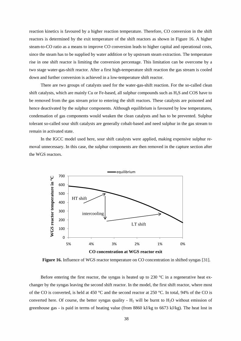
Figure 16. Influence of WGS reactor temperature on CO concentration in shifted syngas. ................. 38
Figure 17. Schematics of physical absorption process with Selexol..................................................... 41
Figure 18. Acid gas concentrations in absorber with MDEA at a rich loading of 0.8. ......................... 45
Figure 19. Desorption behaviour of MDEA. ........................................................................................ 46
Figure 20. Process flowsheet of IGCC with acid gas removal. ............................................................ 49
Figure 21. Pre-combustion H2S capture section with Selexol. ............................................................. 53
Figure 22. Pre-combustion CO2 capture section with Selexol. ............................................................. 54
Figure 23. Flowsheet for pre-combustion co-capture installation with Selexol. .................................. 56
Figure 24. Pulverised coal power plant with amine CO2 capture and other emission controls.. .......... 61
Figure 25. Process flow diagram for CO2 capture by chemical absorption .......................................... 62
Figure 26. Absorption section for post-combustion CO2 scrubbing ..................................................... 67
Figure 27. CO2 removal eff. at 20 °C of MEA, DGA, and NH3 at different solvent-to-CO2 ratios. ..... 68
Figure 28. Schematic diagram of non-regenerative CO2 capture with ammonia. ................................. 70
vii
Figure 29. Ammonia salt formation for different loadings (mol/mol) of the ammonia solvent. .......... 71
Figure 30. Schematic diagram of semi-continuous flow absorber for CO2. ......................................... 72
Figure 31. CO2 removal efficiency by ammonia solution (5% wt.) at different temperatures.............. 74
Figure 32. Salts produced in EAA solution at different NH3 concentrations for T = -5 °C. ................. 76
Figure 33. Salts produced in EAA solution at different NH3 concentrations for T = -5 °C .................. 76
Figure 34. CO2 capture efficiency of AA and EAA solutions at 20 °C with 5% wt. NH3. ................... 77
Figure 35. Comparison of simulations to experiments with AA and EAA solution at T = 20 °C. ....... 78
Figure 36. Regeneration efficiency for the investigated solvents at different reboiler temperatures. .. 79
Figure 37. Flowsheet for rate-based model of CO2 removal with ammonia solvent. ........................... 82
Figure 38. Temperature and absorption rate in absorber column with NH3 solvent (T = 1.7 °C). ....... 83
Figure 39. Temperature and absorption rate in intercooled absorber with NH3 solvent (T = 1.7 °C)... 83
Figure 40. Removal efficiency for different solvent flows (T = 1.7 °C) and concentrations (% wt.)... 84
Figure 41. Relative NH3 desorption eff. for varying desorber conditions compared to base case. ....... 85
Figure 42. CO2 removal efficiency for different molar and mass flows of ammonia and MEA. ......... 87
Figure 43. Flowsheet for rate-based model of CO2 removal with MEA. .............................................. 89
Figure 44. Temperature and absorption rate profiles in absorber column with MEA solvent. ............. 90
Figure 45. Temperature and absorption rate in intercooled absorber column with MEA solvent. ....... 91
Figure 46. CO2 removal efficiency for different solvent flows and MEA concentrations (% wt.). ...... 91
Figure 47. Relative MEA desorption eff. for varying desorber conditions compared to base case. ..... 92
Figure 48. Cryogenic air separation unit. .............................................................................................. 98
Figure 49. Schematic diagram of 500 MW ASC PC oxy-fuel power plant. ....................................... 100
Figure 50. Three-column ASU with two levels of air compression. .................................................. 101
Figure 51. Reactive pre-compression of CO2. .................................................................................... 104
Figure 52. Base case for CO2 purification. ......................................................................................... 107
Figure 53. CO2 purification (Air Products) with stripper column at 17 bar. ....................................... 108
Figure 54. CO2 purification (Air Products) with stripper column at 30 bar. ....................................... 109
Figure 55. T-Q Diagram for Air Products cold box (dTmin = 1 °C) with stripper column at 30 bar. .. 110
Figure 56. CO2 purification (Air Liquide) with distillation column. .................................................. 111
Figure 57. CO2 purification (Praxair) without distillation column. .................................................... 112
Figure 58. Life cycle stages. ............................................................................................................... 116
Figure 59. Life Cycle Assessment phases. .......................................................................................... 118
Figure 60. Midpoint versus endpoint modelling. ................................................................................ 120
Figure 61. Principles of the Eco-indicator method. ............................................................................ 121
Figure 62. LCA boundaries for PC power plant a) without CO2 capture and b) with capture............ 125
Figure 63. LCA boundaries for IGCC a) without acid gas removal and b) with removal. ................. 126
Figure 64. LCA process flow diagram for the production of 1 kg of MEA........................................ 128
Figure 65. Influence of LCA phases on weighted results of PC power plant without CO2 capture. .. 131

viii
Figure 66. Impact of GHG emissions for IGCC with and without acid gas removal. ........................ 133
Figure 67. Impact of GHG emissions for PC power plant with and without CO2 capture. ................ 133
Figure 68. Impact of GHG emissions for oxy-fuel power plant with CO2 purification. ..................... 134
Figure 69. Impacts of resource consumption for IGCC with and without acid gas removal. ............. 135
Figure 70. Impacts of resource consumption for PC power plant with and without CO2 capture. ..... 135
Figure 71. Impacts of resource consumption for oxy-fuel power plant with CO2 purification. ......... 136
Figure 72. Environmental impacts IGCC with and without acid gas removal. .................................. 137
Figure 73. Environmental impacts of PC power plant with and without CO2 capture. ...................... 137
Figure 74. Environmental impacts of oxy-fuel power plant with and without CO2 purification. ....... 138
Figure 75. Potential environmental damages caused by IGCC with and without acid gas removal. .. 139
Figure 76. Potential environmental damages caused by PC plant with and without CO2 capture. ..... 139
Figure 77. Potential environmental damages caused by oxy-fuel plant with CO2 purification. ......... 140
Figure 78. Main exergy stream for IGCC with and without acid gas removal. .................................. 145
Figure 79. Main exergy stream for PC power plant with and without CO2 capture. .......................... 146
Figure 80. Main exergy stream for oxy-fuel power plant with CO2 purification. ............................... 148
Figure 81. Life cycle irreversibilities of IGCC with and without acid gas removal. .......................... 152
Figure 82. Life cycle irreversibilities of PC power plant with and without CO2 capture. .................. 153
Figure 83. Life cycle irreversibilities of oxy-fuel power plant with CO2 purification. ....................... 154

ix
List of Tables
Table 1. Characteristics of greenhouse gases. ....................................................................................... 16
Table 2. GHG emissions from fuel combustion and reduction targets for Kyoto parties. .................... 22
Table 3. GHG emissions from fuel combustion and for non-Kyoto parties and worldwide. ............... 23
Table 4. Current cost ranges for CCS system components. .................................................................. 30
Table 5. Worldwide CCS Projects in operation. ................................................................................... 31
Table 6. Properties of coal used in IGCC for equilibrium pre-combustion capture models. ................ 36
Table 7. Component yields for pyrolysis in IGCC model for equilibrium pre-combustion capture. ... 36
Table 8. IGCC operation parameters. ................................................................................................... 37
Table 9. Properties of Selexol at T = 25 °C. ......................................................................................... 40
Table 10. Properties of MDEA at T = 20 °C. ....................................................................................... 43
Table 11. Equilibrium constants for absorption reactions with MDEA. ............................................... 44
Table 12. Rate constants for kinetic reactions. ..................................................................................... 44
Table 13. Henry constants of acid gas components in water. ............................................................... 45
Table 14. Compositions and heating values of gas streams in IGCC with acid gas capture. ............... 47
Table 15. Parameters for IGCC with capture of CO2 and H2S. ............................................................ 48
Table 16. Properties of coal used in IGCC for rate-based pre-combustion capture models. ................ 50
Table 17. Component yields for pyrolysis in IGCC model for rate-based pre-combustion capture. .... 50
Table 18. IGCC operation parameters. ................................................................................................. 51
Table 19. Equilibrium constants for grey water wash........................................................................... 51
Table 20. Key parameters of rate-based H2S capture and CO2 capture sections with Selexol. ............ 55
Table 21. Key parameters of rate-based co-capture section with Selexol. ........................................... 57
Table 22. Composition and flow of gas streams. .................................................................................. 57
Table 23. Composition and flow of burned gas streams. ...................................................................... 58
Table 24. Parameters for IGCC with and without pre-combustion capture of CO2 and H2S................ 59
Table 25. Coal analysis for PC power plant. ......................................................................................... 65
Table 26. PC power plant parameters. .................................................................................................. 65
Table 27. Flue gas composition of PC power plant. ............................................................................. 66
Table 28. Equilibrium constants for absorption with MEA, DGA, and NH3........................................ 68
Table 29. Ammonia salt solubilities. .................................................................................................... 71
Table 30. Development of component concentrations (% wt.) in 5 %wt. ammonia solution. .............. 74
Table 31. Development of component concentrations (%wt.) in EAA solution. .................................. 75
Table 32. Solvents for equilibrium-based post-combustion capture simulations and experiments. ..... 78
Table 33. Key parameters of CO2 capture installation (one of four) with ammonia solvent. ............... 86
x
Table 34. Rate constants for kinetic reactions. ..................................................................................... 88
Table 35. Key parameters of CO2 capture installation (one of four) with MEA solvent. ..................... 89
Table 36. Stream data for post-combustion CO2 capture with MEA and ammonia. ............................ 93
Table 37. Parameters for 500 MW PC power plant with and without CO2 capture. ............................ 95
Table 38. CO2 purity issues for storage and for use in EOR. ................................................................ 99
Table 39. Oxy-fuel power plant parameters. ....................................................................................... 102
Table 40. Reactions in reactive compression with distillation. ........................................................... 104
Table 41. Flue gas parameters in CO2 pre-compression. .................................................................... 106
Table 42. Stream compositions for the investigated CO2 purification systems. ................................. 113
Table 43: Parameters for Oxy-fuel power plant with cryogenic CO2 purification. ............................ 114
Table 44. Weighting factors in Eco-indicator 99 method. .................................................................. 122
Table 45. Damage categories and weighting factors in Eco-indicator 99 method. ............................. 122
Table 46. Life Cycle Inventory (LCI) of investigated power plant structures. ................................... 127
Table 47. Waste management for materials used in power plants. ..................................................... 129
Table 48. Uncertainty of characterised LCA results for PC power plant with MEA scrubbing. ........ 130
Table 49. Exergies of main energy and mass flows of IGCC. ............................................................ 146
Table 50. Exergies of main energy and mass flows of PC power plant. ............................................. 147
Table 51. Exergies of main energy and mass flows of oxy-fuel power plant. .................................... 148
Table 52. Exergy destruction ĖD and exergetic efficiencies of all power plant configurations. ......... 150
Table 53. Cumulative exergy consumption of resources and utilities for plant construction. ............ 151
Table 54. CExC and end-of-life irreversibilities related to power plant construction. ....................... 151
Table 55. Technical, environmental, and exergo-environmental performance of capture options. .... 157
Table 56. Overview of advantages and disadvantages of studied capture processes. ......................... 158
xi
Nomenclature
a Stoichiometric coefficient
AA Aqueous ammonia
aMDEA Activated MDEA process, licensed by BASF
ASC Advanced supercritical
ASU Air separation unit
CAP Chilled ammonia process
CCS Carbon capture and storage
CExC Cumulative exergy consumption
d Change (delta)
DALY Disability adjusted life years
DGA Diglycolamine
DEPG mixture of dimethyl ethers of polyethylene glycols
e Specific exergy
E Exergy
Ė Exergy stream
EAA Aqueous ethanol-ammonia solvent
EC European Community
EGR Enhanced gas recovery
ELCA Exergy life cycle assessment
EOR Enhanced oil recovery
EOS Equation of state
ESP Electrostatic precipitator
FG Flue gas
FGD Flue gas desulphurisation
FSU Former Soviet Union
G Gibbs free energy
GE General Electrics
GHG Greenhouse gases
GT Gas turbine
GWP Global warming potential
h Specific enthalpy
H Enthalpy
H&MB Heat and mass balances
HE Heat exchanger
HHV Higher heating value
HP High pressure

xii
HRSG Heat recovery steam generator
İ Irreversibility
IEA GHG IEA Greenhouse Gas R&D programme
IGCC Internal gasification combined cycle
IP Intermediate pressure
IPCC International Panel on Climate Change
ISO International Standards Organization
K Equilibrium constant
KEPCO Kansai Electric Power Company
KS-1 Proprietary hindered amine solvent from KEPCO/MHI
k pre-exponential kinetic factor
LCA Life-cycle assessment or life-cycle analysis
LCI Life-cycle inventory
LCIA Life-cycle impact assessment
LCM Life-cycle management
LP Low pressure
LULUFC Land use, land-use change and forestry
LHV Lower heating value
m Mass flow
MDEA Methyl-diethanolamine
MEA Monoethanolamine
MHI Mitsubishi Heavy Industries
n Mole flow
NGCC Natural gas combined cycle
NMR Nuclear magnetic resonance spectroscopy
NRTL Non-Random Two-Liquid activity coefficient model
OC Other countries
OECD Organisation for Economic Co-operation and Development
OME Other major economies
p Pressure
pi Partial pressure
PAF Potentially affected fraction
PC Pulverised coal
PC-SAFT Perturbed chain statistical associating fluid theory
PDF Potentially disappeared fraction
ppb Parts per billion
ppm Parts per million
PR-BM Peng-Robinson equation of state with Boston-Mathias correction
r Reaction rate

xiii
Rectisol Commercial name for physical solvent methanol
RK Redlich-Kwong equation of state
s Specific entropy
S Entropy
SCR Selective catalytic reduction
SD Standard deviation
Selexol Mixture of dimethyl ethers of polyethylene glycol
SETAC Society of environmental toxicology
SOFC Solid oxide fuel cell
ST Steam turbine
UNEP United Nations Environment Programme
UNFCCC United Nations Framework Convention on Climate Change
VLE Vapour-liquid equilibrium
Ẇ Work stream
WEO World Energy Outlook (Models and Scenarios by the IEA)
WGS Water-gas-shift
x mole fraction
Greek letters
α Activity coefficient
ε Simple exergy efficiency
ψ Rational exergy efficiency
Subscripts
0 Standard or environmental state
ch Chemical
D Destruction
i Component i
in Incoming
mix Mixing
out Outgoing
ph Physical
q Heat

14
1. Climate change
The effect of human action on the climate is now widely accepted. In this chapter the major
causes of global warming by greenhouse gases such as CO2 and its effect on the environment will be
discussed, with the focus on its industrial origins. Here, power generation by fossil fuels is the promi-
nent contribution [1]. For this sector then technical solutions for the mitigation of greenhouse gases
will be presented.
1.1. Climate change by global warming
The IPCC defines climate change as the state of the climate that can be identified by changes in
the mean value and/or the variability of its properties, and that persists for an extended period, typi-
cally decades or longer. It refers to any change in climate over time, whether due to natural variability
or as a result of human activity [2]. In contrast, the UNFCCC uses a definition, which attributes cli-
mate change directly or indirectly to human activity that alters the composition of the global atmos-
phere in addition to natural climate variability observed over comparable time periods [3].
As presented in Figure 1, it can be observed that the linear warming trend for the 50 years be-
tween 1956 and 2005 is nearly twice as steep as that for the 100 years between 1906 and 2006. This
trend is especially pronounced in the northern hemisphere. The average arctic temperatures have in-
creased with almost twice the average global rate over the past 100 years. Sea levels have risen ac-
cordingly, a major contribution, 57% since 1993, being the thermal expansion of the oceans, while the
melting of glaciers and ice caps contributed with 28% over the same period.
These stated changes have observable impacts on the environment. For natural systems related
to snow, ice and frozen ground, it is observed that glacial lakes have increased in number and exten-
sion, permafrost regions show increasing ground instability, rock avalanches in mountain regions
have increased in number. For terrestrial biological systems there is very high confidence that a wide
range of species is affected by earlier spring events. Marine and freshwater biological systems are af-
fected by rising water temperatures, changes in ice cover, salinity, oxygen levels and circulation [2].

15
Figure 1. Observed changes in global average surface temperature, global average sea level, and
Northern hemisphere snow cover for March-April with decadal averaged values (curves),
yearly values (dots) and uncertainty intervals (shaded) [2].
Global warming is caused by natural and anthropogenic drivers, the emission of long-lived
greenhouse gases (GHG) being the major contribution. GHGs contribute to global warming by chang-
ing the radiation balance of the earth. While the existence of greenhouse gases is important for the
thermal balance of the earth by preventing the release of all reflected solar radiation from the earth's
surface, the increased emission of these gases leads to a lower release of the infrared part of the spec-
trum and thus to an increase in the earth's temperature as shown in Figure 2. This effect of altering the
balance of incoming and outgoing energy in the earth-atmosphere system is often measured with the
radiative forcing value. This value in W/m2 is an index standing for the importance of a potential cli-
mate change mechanism and is used in the IPCC reports for changes relative to pre-industrial condi-
tions defined at 1750 [2].
Anthropogenic GHG emissions have increased globally by about 70% between 1970 and 2004.
Due to their different radiative properties and lifetimes in the atmosphere the warming influence of
16
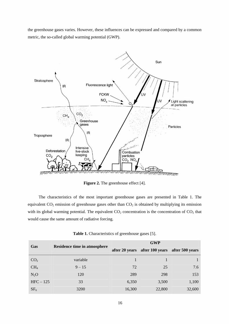
the greenhouse gases varies. However, these influences can be expressed and compared by a common
metric, the so-called global warming potential (GWP).
Figure 2. The greenhouse effect [4].
The characteristics of the most important greenhouse gases are presented in Table 1. The
equivalent CO2 emission of greenhouse gases other than CO2 is obtained by multiplying its emission
with its global warming potential. The equivalent CO2 concentration is the concentration of CO2 that
would cause the same amount of radiative forcing.
Table 1. Characteristics of greenhouse gases [5].
Gas Residence time in atmosphere GWP
after 20 years after 100 years after 500 years
CO2 variable 1 1 1
CH4 9 – 15 72 25 7.6
N2O 120 289 298 153
HFC – 125 33 6,350 3,500 1,100
SF6 3200 16,300 22,800 32,600

17
The observed increase in global average temperatures over the last 100 years is very likely due
to the increase in anthropogenic GHG emissions as shown in Figure 4.
Figure 3. Observed decadal averages of surface temperature with overlay of uncertainty bands
for climate models with and without anthropogenic GHG emissions [6].
In Figure 4, the emission of anthropogenic GHGs is shown in terms of CO2 equivalents for the
years 1974 to 2004. For 2004, the distribution of GHG emissions across the different sectors of an-
thropogenic activity is given. It is obvious that the most important greenhouse gas is CO2, while the
emissions are caused mainly by the industrial sector, in particular the energy supply. The still rising
demand for energy and the increase in CO2 emissions typically involved has become one of the most
important environmental topics. Coal is a resource still readily available. Its use in power generation
comes with a cost, however. The combustion or gasification of coal releases a high amount of CO2.

18
Figure 4. a) Global annual emissions of anthropogenic GHGs,
b) share of different sectors in total anthropogenic GHG emissions in 2004 in CO2-eq [2].
It is obvious that without a change in policy global warming will increase further and thus will
have major environmental and social effects caused by extreme weather and climate events.

19
1.2. Responding to climate change
1.2.1. Alternative responses
There are two possible responses to climate change. One of them is the adaptation to its effects
and the other, also called mitigation, is the reduction of GHG emissions in order to reduce the rate and
magnitude of climate change. The possibility to adapt to climate change is limited and dependent on
the society's financial, technological, political, and cultural resources. However, even highly adaptive
societies are vulnerable to extremes such as the heat wave in Europe in 2003 and hurricane Katrina in
the United States in 2005, both causing large human costs.
An important factor for the implementation of mitigation options is the regional environmental
and socio-economic situation and the availability of information and technology. In order for this op-
tion to be effective, a concerted global approach needs to be taken.
1.2.2. Objectives of the Kyoto Protocol
For establishing a global response to climate change, the environmental treaty UNFCCC was
produced at the United Nations Conference on Environment and Development (UNCED) in Rio de
Janeiro in 1992 and entered into force in 1994, ratified by over 50 countries. The treaty, although con-
sidered legally non-binding, requires for updates called "protocols". Since 1995, the UNFCCC coun-
tries meet annually in Conferences of the Parties (COP). The principal update, the Kyoto Protocol,
established national greenhouse gas inventories and created the 1990 benchmark of national green-
house gas emissions. The Kyoto Protocol was concluded in 1997 and established legally binding obli-
gations in the Annex I countries for a reduction of GHG emissions (CO2, CH4, N2O, SF6) as well as
the emissions of hydrofluorcarbons and perfluorcarbons from 1990 levels by an average of 5% over
the period 2008-2012. The states that signed the Kyoto Protocol can be divided in three groups. The
industrialised countries committed to complying with the emission targets form the Annex I group. A
subgroup of these countries that pays for costs arising in developing countries is formed by the Annex
II states. These are OECD members except those countries that were economies in transition in 1992.
The third group of countries, the developing countries, are not required to reduce GHG emissions to
avoid restrictions to their development. They can sell emission credits to nations with difficulty of
meeting the emission targets and receive financial and technological help for the implementation of
20
low-carbon technologies. Developing countries may volunteer to become Annex I countries when
they are sufficiently developed [7].
Emission restrictions do not include international shipping and aviation. These limits are inte-
grated in the 1987 Montreal Protocol on Substances that deplete the Ozone Layer with the industrial
gases chlorofluorocarbons, or CFCs [7].
At the 2008 UNFCCC COP 14 in Poznan, Poland, the following objective was formulated [8]:
“The ultimate objective of this Convention and any related legal instruments that the
Conference of the Parties may adopt is to achieve, in accordance with the relevant provi-
sions of the Convention, stabilization of greenhouse gas concentrations in the atmosphere
at a level that would prevent dangerous anthropogenic interference with the climate sys-
tem. Such a level should be achieved within a time frame sufficient to allow ecosystems to
adapt naturally to climate change, to ensure that food production is not threatened and to
enable economic development to proceed in a sustainable manner.”
In November 2009, 186 countries and one regional economic organisation, the EU, have signed
and ratified the Kyoto protocol, representing over 63.9% of the 1990 emissions from Annex I coun-
tries. The United States, which are a signatory of UNFCCC and responsible for 36.1% of the 1990
emission levels, are still a non-member. India and China are excluded from complying with the emis-
sion limits, as they are considered developing countries despite a massive increase of their GHG
emissions.
The so far 37 Annex I countries that agreed to binding emission targets may only exceed their
allocations if they buy emission allowances or take other measures that all UNFCCC parties have to
agree upon. The Kyoto Protocol allows for so-called flexible mechanisms that enable Annex I coun-
tries to acquire GHG emission credits either by financing emission reducing projects in other Annex I
or non-Annex I countries or by purchasing credits from Annex I countries with excess credits [7].
These mechanisms are:
Emissions Trading (ET):
Countries with permitted but "unused" emissions may sell this excess capacity to coun-
tries that are exceeding their emission targets. Carbon dioxide being the principal green-
house gas, a so-called carbon market has been created, on which emission permits are
now tracked and traded like any other commodity.
21
Clean Development Mechanism (CDM):
A country with an emission limit commitment under the Kyoto Protocol may implement
an emission-reduction project in developing countries. With such projects saleable certi-
fied emission reduction (CER) credits can be acquired. A CDM project activity can be,
for example, a rural electrification project with solar panels or the installation of more
energy-efficient boilers.
Joint Implementation (JI):
Emission reduction units (ERUs) can be acquired from an emission-reduction or emis-
sion removal project in another Annex I country, from which the host country benefits by
investment and technology transfer.
At the COP 15 United Nations climate Change Conference in Denmark a global climate agree-
ment was to be established due to the near expiration of the first commitment period of the Kyoto Pro-
tocol in 2012. However, only a less specific politically binding agreement was reached, postponing a
binding post-Kyoto agreement to a second summit meeting in Mexico City to be held in December
2010 [7].
For countries that ratified the Kyoto protocol, the development of GHG emissions from fuel
combustion is shown in Table 2. On average, in 2007 the participating countries were below the
specified emission limits of the Kyoto Protocol, but recent increases in emissions may threaten the
compliance with the set targets. While the 36 Kyoto countries are on pace to meet the 5% reduction
target by 2012, most of the emission reduction is due to the decline in the Eastern European countries'
emissions after the collapse of communism in the 1990s.
The overall target of emission reduction in the EU under the Kyoto Protocol is 8% from 1990
levels by 2008-2012. However, the GHG reduction targets of the EU and member countries were
agreed on in June 1998 under the so-called "Burden Sharing Agreement" specified in the EC ratifica-
tion decision. The reduction targets specified under this agreement are generally stricter than the orig-
inally fixed targets under the Kyoto Protocol.

22
Table 2. GHG emissions from fuel combustion and reduction targets for Kyoto parties [9].
Country 1990 2007 change
1990-2007
Reduction
target
KYOTO PARTIES 8792.2 8162.1 -7.2% -4.7%
North America 432.3 572.9 32.5% -6%
Canada 432.3 572.9 32.5% -6%
Europe 3158.7 3281.3 3.9% (-8%)
Austria 56.2 69.7 24.0% -13.0%
Belgium 107.9 106.0 -1.8% -7.5%
Denmark 50.4 50.5 2.0% -21.0%
Finland 54.4 64.4 1.9% 0.0%
France 352.1 369.3 4.9% 0.0%
Germany 950.4 798.4 -16.0% -21.0%
Greece 70.1 97.8 39.5% 25.0%
Iceland 1.9 2.3 24.6% 10.0%
Ireland 30.6 44.1 44.1% 13.0%
Italy 397.8 437.6 10.0% -6.5%
Luxembourg 10.5 10.7 2.5% -28.0%
Netherlands 156.6 182.2 16.4% -6.0%
Norway 28.3 36.9 30.6% 1.0%
Portugal 39.3 55.2 40.5% 27.0%
Spain 205.8 344.7 67.5% 15.0%
Sweden 52.8 46.2 -12.4% 4.0%
Switzerland 40.7 42.2 3.6% -8.0%
United Kingdom 533.0 523.0 -5.4% -12.5%
Pacific 1346.5 1668.1 23.9%
Australia 259.8 396.3 52.5% 8.0%
Japan 1065.3 1236.3 16.1% -6.0%
New Zealand 21.3 35.5 66.4% 0.0%
Economies in transition 3854.7 2639.8 -31.5%
Bulgaria 74.9 50.2 -33.0% -8.0%
Croatia 22.0 22.0 2.1% -5.0%
Czech Republic 155.4 122.1 -21.4% -8.0%
Estonia 36.2 18.0 -50.1% -8.0%
Hungary 66.7 53.9 -19.1% -6.0%
Latvia 18.4 8.3 -54.6% -8.0%
Lithuania 33.1 14.4 -56.4% -8.0%
Poland 343.7 304.7 -11.4% -8.0%
Romania 167.1 91.9 -45.0% -8.0%
Russian Federation 2179.9 1587.4 -27.2% 0.0%
Slovak Republic 56.7 36.8 -35.1% -8.0%
Slovenia 13.1 15.9 21.2% -8.0%
Ukraine 687.9 314.0 -54.4% 0.0%

23
When looking at the development of GHG emissions of the non-Kyoto parties and of world-
wide emissions as shown in Table 3, it becomes obvious that efforts to reduce these emissions are
crucial.
Table 3. GHG emissions from fuel combustion and for non-Kyoto parties and worldwide [9].
Country 1990 2007 change
1990-2007
Reduction
target
NON-KYOTO PARTIES 11577.8 19778.3 70.8%
Non-participating
Annex I Parties 5106.3 6097.0 19.4%
Belarus 116.1 62.7 -46.0%
Turkey 126.9 265.0 1.1%
United States 4863.3 5769.3 18.6% -7.0%
Other regions 6471.5 13681.3 111.4%
Africa 546.2 882.0 61.5%
Middle East 588.2 1389.0 136.1%
Non-OECD Europe 106.1 91.4 -13.9%
Other FSU 581.6 406.7 -30.1%
Latin America 897.0 1453.9 62.1%
Asia (excl. China) 1508.4 3387.1 124.6%
China 2224.0 6071.2 170.6%
Int. Marine Bunkers 356.9 610.4 71.1%
Int. Aviation Bunkers 253.6 411.6 62.3%
World 20980.5 28962.4 38.0%
In Figure 5 the development of international GHG emissions is presented graphically, high-
lighting the importance of emissions by non-Annex I parties.
Figure 5. Development of GHG emissions worldwide [9].

24
In the context of this work, it is important to note that the energy sector is the major contributor
to anthropogenic GHG emissions, especially in the Annex I countries. For the year 2006, the distribu-
tion of GHG emissions over the different sectors is shown in Figure 6, excluding land use, land-use
change and forestry (LULUFC).
Figure 6. Anthropogenic GHG emissions without LULUFC in Annex I parties for 2006 [1].
The strong contribution of the energy sector to GHG emissions is caused by the extensive use
of fossil fuels. In Figure 7 the projected development of worldwide primary energy consumption ac-
cording to the reference scenario in the World Energy Outlook model (WEO) by the IEA is shown.
Figure 7. World primary energy demand in the Reference Scenario [10].
According to this model, non-OECD countries, here especially India and China, are responsible
for 93% of the increase in global energy demand between 2007 and 2030. For this reference scenario,
77% of this increase is caused by fossil fuel consumption as presented in Figure 8.

25
Figure 8. Change in global primary energy demand between 2007 and 2030 by fuel type [10].

26
1.3. Mitigation options
If the global temperature rise is to be limited, mitigation has to be applied with an ample portfo-
lio of technologies. The reference scenario predicts a temperature rise of 6 °C. So limiting the tem-
perature rise to 2°C requires big emission reductions in all regions and sectors. There is large uncer-
tainty concerning the future contribution of the different mitigation technologies. The different stabili-
sation scenarios foresee that 60 to 80% of GHG emission reductions will be achieved in the sectors of
energy supply and industrial processes. Emphasis is laid on higher efficiency and the use of low-
carbon energy sources, which include the shift from coal to gas-fired power plants and the increased
use of renewables. Including LULUFC mitigation options, such as reforestation, improved crop yields
with reduced use of fertilizers, and manure management for decreased release of CH4, allows for
greater flexibility and cost-effectiveness [10].
In the WEO 450 Scenario, with a stabilisation of atmospheric CO2 concentration to 450 ppm,
demand for fossil fuels will peak by 2020, and by 2030 zero-carbon fuels will contribute to a third of
the world's primary sources of energy demand. In this scenario, improved energy efficiency will ac-
count for most of the abatement as shown in Figure 9.
Figure 9. Role of abatement technologies in 450 scenario for OECD countries, other major econo-
mies (OME) and other countries (OC) compared to reference scenario [10].
In the context of this work, it should be stressed that renewables, nuclear power plants and
plants fitted with carbon capture and sequestration account for around 60% of global electricity gen-
eration in 2030 in the 450 scenario, while today it is only one third. There would be additional bene-
fits to energy security by reduced oil and gas imports, and less air pollution.

27
1.3.1. Importance of fossil fuels
Modern economies strive for securing energy supply by safe and stable power generation as
well as independence from importing fossil fuels. More recently climate protection became an impor-
tant factor in the planning of new power plants. Potential solutions such as renewable energies will
not be able to secure our actual (and growing) need of power in the near future. Coal, however, will
be available in Europe for about another 400 years. It is also an important fuel in fast-growing
economies such as in China.
Large point sources such as power plants make up about 40% of all anthropogenic CO2 emis-
sions, especially in fast developing countries with large coal reserves. Other important point sources
are sites of the cement and steel industry, fermentation processes for food and ammonia production.
One of the main problems with coal is the high CO2 emission its use causes. In the next section,
an option for reducing the environmental impact of fossil fuel burning is discussed.
1.3.2. Climate change mitigation by Carbon Capture and Storage
In Carbon Capture and Storage (CCS) as a major decarbonisation technology, a concentrated
CO2 stream is produced, which can be transported to an adequate storage site. CCS is an important
mitigation option, since it allows for the continued use of fossil fuels even in scenarios with low GHG
intensity. Large point sources such as power plants are ideal for the application of CCS. Combining
CCS with the use of biomass, e.g. when co-fired in coal power plants, allows for effective net removal
of CO2 from the atmosphere.
The four basic systems for CO2 capture in processes using fossil fuels and/or biomass are pre-
sented in Figure 10. Post-combustion CO2 capture is the capture from flue gases produced by fuel
combustion, while in pre-combustion capture CO2 is removed from a syngas stream to be burned in a
successive process step. The syngas stream is produced by reacting a fuel with air or oxygen. In oxy-
fuel combustion, the fuel is burned with nearly pure oxygen, resulting in a very high concentration of
CO2 in the flue gas stream, which is then concentrated further to allow for storage. These processes
are described in more detail in the corresponding chapters of this thesis. CO2 separation has been ap-
plied for more than 80 years to large industrial plants for natural gas processing and in ammonia pro-
duction [11] In these processes carbon capture is applied to meet process demands and not for storage
due to lack of economical and policy incentives.

28
Figure 10. The four principal systems of CO2 capture [12].
The main CO2 capture technologies (absorption, membrane separation, distillation and cryo-
genic separation) are presented in Figure 11.
Figure 11. The main gas separation processes for CO2 capture [12].

29
The principal disadvantage of CCS is that it energy is required, leading to a reduction in plant
efficiency and increased fuel consumption. The influence of CO2 capture on the latter is shown in
Figure 12. Here, the power plants including CO2 capture are compared to identical plants without cap-
ture
Figure 12. Increase in fuel consumption due to CO2 capture [12].
After the CO2 has been separated from the point source, the captured CO2 may be stored under-
ground, in the deep ocean or by industrial fixation as inorganic carbonates. Injection into geological
storage sites is the most mature storage option. A number of commercial projects are already in opera-
tion. The other mentioned options show important disadvantages. Deep sea storage may not retain the
CO2 permanently and its ecological impacts are still unclear. Industrial fixation in mineral carbonates
is very costly and requires a large amount of energy [13]. Total estimates for geological storage of
CO2 range from 1,000 to 10,000 Gt of CO2, which represents more than 26 to 260 times the projected
energy related emissions in 2030 [14, 9]. Storage may occur in depleted oil and gas reservoirs (920 Gt
CO2), saline aquifers (400 - 10,000 Gt CO2) and unminable coal seams (40 Gt CO2) [15]. The integ-
rity of these storage sites needs to be ensured to prevent the possibly dangerous and at least counter-
productive release of the stored gases. Most screening activities to explore adequate reservoirs are
concentrated in North America, Europe, Japan and Australia due to political commitments there to
reduce CO2 emissions. Apart from storage, the CO2 may also be used in industrial processes, e.g. for
the production of methanol or fertilizers.
The drop in energy efficiency of the power plant due to CO2 capture, the transport of the sepa-
rated CO2 stream and the storage of the captured gases lead to elevated costs. These costs per captured
ton of CO2 are listed in Table 4. However, as the large ranges show, such cost estimates are subject to
assumptions and data inconsistencies. These estimates may also vary over time and depend on loca-
tion and selected technology.
30
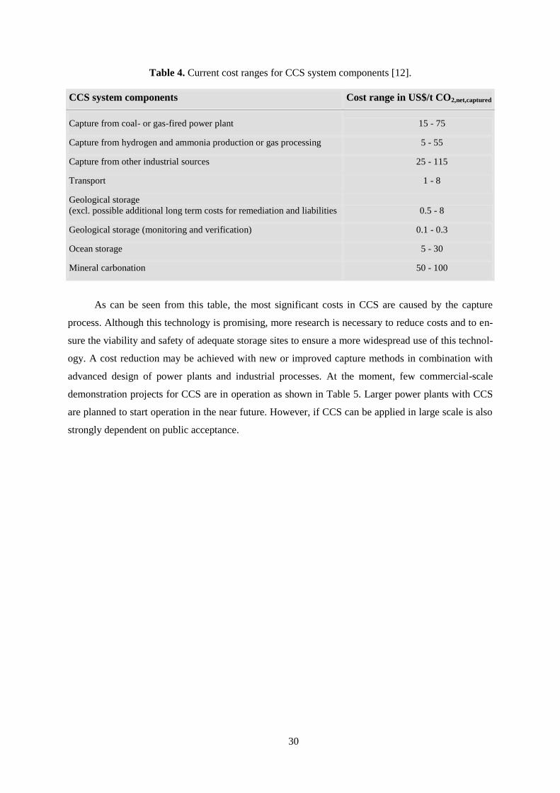
Table 4. Current cost ranges for CCS system components [12].
CCS system components Cost range in US$/t CO2,net,captured
Capture from coal- or gas-fired power plant 15 - 75
Capture from hydrogen and ammonia production or gas processing 5 - 55
Capture from other industrial sources 25 - 115
Transport 1 - 8
Geological storage
(excl. possible additional long term costs for remediation and liabilities 0.5 - 8
Geological storage (monitoring and verification) 0.1 - 0.3
Ocean storage 5 - 30
Mineral carbonation 50 - 100
As can be seen from this table, the most significant costs in CCS are caused by the capture
process. Although this technology is promising, more research is necessary to reduce costs and to en-
sure the viability and safety of adequate storage sites to ensure a more widespread use of this technol-
ogy. A cost reduction may be achieved with new or improved capture methods in combination with
advanced design of power plants and industrial processes. At the moment, few commercial-scale
demonstration projects for CCS are in operation as shown in Table 5. Larger power plants with CCS
are planned to start operation in the near future. However, if CCS can be applied in large scale is also
strongly dependent on public acceptance.

31
Table 5. Worldwide CCS Projects in operation [12, 15, 16, 17, 18, 19, 20, 21].
CCS project Operator Description Technology Projected
cost
Sleipner West
(Norway) Statoil
and IEA
Injection of 1 Mt/yr of CO2
from natural gas field into sa-
line aquifers since 1996
Physical absorption
with Rectisol in gas
cleanup train
€ 350 M
Weyburn
(Canada) EnCana
and IEA
Capture in the Great Plains
synfuels plant in Beulah, ND,
USA, transport by 325 km
pipeline, injection of 7 Mt of
CO2 from 2000 to 2004, cur-
rently investigation of long-
term sequestration suitability
Physical absorption
with Rectisol, use
of CO2 for EOR
pipeline cost:
US$ 100 M
In Salah
(Algeria) Sonatrach,
BP, Statoil
Injection of 1 Mt/yr of CO2
from natural gas production to
a total 17 Mt into depleted gas
reservoirs since 2004
Chemical absorp-
tion with aMDEA
US$ 1700 M
K12B
(Netherlands) Gaz de France Injection of CO2 from natural
gas production into the original
gas reservoir (1 - 1.5 Billion
m3) since 2004
Chemical absorp-
tion with aMDEA,
use of CO2 for EGR
n/a
Snøhvit
(Norway) Statoil Injection of CO2 from natural
gas production beneath seabed
since 2008, planned: 0.7 Mt/yr
n/a total:
$US 5200 M,
injection:
US$ 110 M
La Barge
(Wyoming) ExxonMobil Injection of 4 Mt/yr of CO2
from natural gas production
into depleted gas reservoirs
Two-train physical
acid gas removal
with Selexol
n/a
Ketzin
(CO2SINK)
(Germany)
GFZ Potsdam Storage of CO2 in saline aqui-
fers since 2008, planned: 60 kt
over 2 years
CO2 from industrial
gas supplier
€ 15 M
Schwarze Pumpe
(Germany) Vattenfall Capture of up to 100 kt CO2
from 30 MW coal-fired power
plant since 2008, storage in
depleted gas field planned
Oxyfuel, 98% CO2
purity
€ 70 M

32
2. Pre-combustion capture
Pre-combustion CO2 capture is the separation of CO2 from the fossil fuel before combustion.
For an efficient capture, the fossil fuel is first converted into CO2 and hydrogen gas. For natural gas,
the conversion of the fuel into synthesis gas is achieved in a traditional steam reformer. Then, the car-
bon monoxide in the syngas reacts with steam and forms CO2, as all remaining carbon monoxide is
later burned to CO2. As for coal used in an Internal Gasification Combined Cycle (IGCC), after gasi-
fication it is converted into CO2 and H2 in a water-gas-shift reaction.
2.1. Comparison of pre-combustion capture techniques
Either by membrane processes or in an absorption section, the CO2 is separated from the con-
verted hydrogen rich syngas stream, which is then mixed with air and burned in the combustion
chamber of a gas turbine. The captured carbon dioxide is compressed and liquefied for transport and
storage.
Pre-combustion capture allows for the removal of about 90% of the CO2 from a power plant.
However, this technology requires significant modifications of the power plant and is thus only viable
for new plants. The investment costs for an IGCC with CO2 capture is about twice as high as for a
similar plant using post-combustion capture [22] as discussed in the next chapter.
Capture costs may be reduced in the future through improved gasification technology and
through improved performance of the capture process. Highly selective membranes and ionic liquid
membranes for this purpose are at the laboratory stage of development [23, 24, 25]. Furthermore,
power plant efficiency may be improved by the integration of power fuel cells (SOFC) that use the
H2-rich syngas [26]. If economically feasible, part of the produced hydrogen can also be stored and
sold as fuel.
Even though large-scale demonstration plants exist, highly efficient hydrogen turbines, which
are optimised for CCS, are still under development [27, 28].
In case of IGCC, apart from CO2, the acid gas component H2S also has to be removed to pre-
vent formation of SO2 in the combustion process, which would then be released with the flue gas
stream. For acid gas removal by absorption, the available solvents can be divided in three groups. In
physical solvents such as Selexol or methanol, absorption occurs according to Henry's law, so that the
solubility of an acid gas in physical solvents increases linearly with its partial pressure [29]. In chemi-
cal solvents, such as monoethanolamine, the acid gas reacts chemically with the solvent. More infor-

33
mation can be found in the chapter on post-combustion capture. The third group, the mixed solvents,
such as sterically hindered amine (MDEA) shows both types of capture, physical and chemical [30].
Physical solvents, such as Rectisol or Selexol, are favoured by a high partial pressure of the
acid gas in the syngas and can be regenerated with lower energy consumption. This is due to the fact
that usually the bulk of the regeneration duty is done by a simple flashing (pressure reduction).
Chemical solvents have higher absorption capacity at relatively low acid gas partial pressures. How-
ever, their absorption capacities plateau at higher partial pressures as shown in Figure 13. Chemical
solvents also require a significant amount of energy, usually in the form of LP steam for regeneration,
because the chemical link between the acid gases and the solvent must be broken. The mixed solvents
display a performance that is a compromise between the first two categories.
Figure 13. Characteristics for physical and chemical solvents [31].
Since the syngas from a gasification process usually is under pressure, physical solvents are at-
tractive. Physical solvents also generally display a better selectivity than chemical solvents, which
would permit to separately capture H2S. This separation permits to convert H2S to sulphur (Claus
process) and to obtain a pure CO2 by-product. The same applies also for mixed solvents and hindered
amines such as MDEA. However, a separate acid gas removal of H2S and CO2 requires higher capital
and operating costs than their combined removal [32] due to the sulphur recovery in a Claus process
and tail gas treatment.
On the other hand, the combined removal produces a CO2 by-product, which is contaminated
with H2S. Therefore, it has to be decided whether or not it would be acceptable and advantageous to
transport and store the combined acid gas stream. Transporting and storing CO2 containing significant
concentrations of H2S and CO2 may be expensive, and these extra costs may be greater than the reduc-
tions in capture costs. Other hurdles may be posed by regulations and permits for the combined stor-
solv
ent
load
ing
partial pressure
physical solvent chemical solvent

34
age. However, H2S can be advantageous for CO2 enhanced oil recovery, since it improves the misci-
bility of CO2. This would also depend on the nature of the oilfield. At the Weyburn field in Canada,
CO2 with about 2% H2S and other sulphur compounds is used for EOR [30].
Other than solely for power production, the hydrogen-rich syngas, from which the CO2 has
been removed, can be used partially or entirely for the production of fuel hydrogen, ammonia, and for
Fischer-Tropsch liquids with a high H:C ratio, where the excess carbon is then made available for
storage [33]. However, this technology will not be discussed in this work.
Figure 14. Schematics of IGCC with CO2 capture, electricity generation, and by-products [12].
IGCC plants, as shown in Figure 14, are generally considered more costly than comparable
pulverised coal (PC) power plants, if no CO2 capture is applied. However, due to the reduced energy
penalty they are considered less costly, if CO2 capture is applied [12].
In this chapter, the performance of a chemical solvent, the tertiary amine MDEA, and the per-
formance of a physical solvent Selexol is investigated and their influence on power plant performance
compared. For a detailed analysis, the IGCC and the capture processes were modelled in Aspen Plus
with and without consideration of the kinetics of chemical bonding and of mass transfer.
35
2.2. Equilibrium pre-combustion capture models
In this section, the performance of acid gas removal with a sterically hindered amine, MDEA, is
compared to syngas sweetening with a physical solvent (Selexol). MDEA requires a lower solvent
circulation rate than physical solvents and the steam consumption for regeneration is lower than for a
true chemical solvent such as MEA. In order to investigate the influence of pre-combustion capture on
power plant performance and to obtain the compositions of the relevant gas streams, models for the
IGCC have been developed as well.
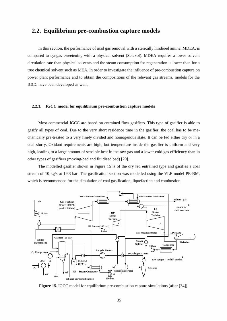
2.2.1. IGCC model for equilibrium pre-combustion capture models
Most commercial IGCC are based on entrained-flow gasifiers. This type of gasifier is able to
gasify all types of coal. Due to the very short residence time in the gasifier, the coal has to be me-
chanically pre-treated to a very finely divided and homogenous state. It can be fed either dry or in a
coal slurry. Oxidant requirements are high, but temperature inside the gasifier is uniform and very
high, leading to a large amount of sensible heat in the raw gas and a lower cold gas efficiency than in
other types of gasifiers (moving-bed and fluidised bed) [29].
The modelled gasifier shown in Figure 15 is of the dry fed entrained type and gasifies a coal
stream of 10 kg/s at 19.3 bar. The gasification section was modelled using the VLE model PR-BM,
which is recommended for the simulation of coal gasification, liquefaction and combustion.
19 bar
Cyclone
Mix-HX
(870 °C)
HP – Steam Generator MP – Steam Generator
LP
Steam
Turbine
Gas Turbine
(Tin = 1350 °C
pout = 1.5 bar)
HP
Steam
Turbine
MP – Steam GeneratorHP – Steam Generator
Reboiler
O2 CompressorRecycle Blower
100 bar
ash
ash and unreacted carbon
Gasifier (19 bar)
air
syngas
(sweetened)
exhaust gas
19 bar
HP Steam (100 bar)
MP Steam (19 bar)
steam for
shift reaction
LP steam
Condenser
Steam
Splitter
raw syngas – to shift section
recycle gas stream
ASU
N2
aircoal
Figure 15. IGCC model for equilibrium pre-combustion capture simulations (after [34]).

36
The amount of oxygen inside the gasification reactor is limited so that only enough of the fuel
is burned to provide the necessary heat for the chemical decomposition of the coal and to produce the
syngas composed mainly of carbon monoxide and hydrogen. The LHV of the reference coal is 23.93
MJ/kg and its composition is presented in Table 6.
Table 6. Properties of coal used in IGCC for equilibrium pre-combustion capture models [34].
Ultimate
analysis
Dry basis Proximate analysis
Dry basis Sulfur
analysis
Dry basis
%wt. %wt. %wt.
Carbon 69.5 Moisture 10 Pyritic 45.7
Oxygen 10 Fixed Carbon (FC) 60 Sulfate 8.86
Nitrogen 1.25 Volatile Matter (VM) 30 Organic 45.7
Hydrogen 5.3 Ash 10
Sulphur 3.95
Chlorine 0
Ash 10
The ash content and the moisture content were both set realistically to 10%. Based on the ulti-
mate analysis, decomposition of the coal was modelled with an RYIELD reactor with the yields
shown in Table 7.
Table 7. Component yields for pyrolysis in IGCC model for equilibrium pre-combustion capture.
H2O C H2 N2 Cl2 S O2 Ash
0.1 0.6255 0.0477 0.01125 0 0.03555 0.09 0.09
The gasifier used 95 %mol pure oxygen (9.2 kg/s, i.e. equivalence ratio of 0.32) at ambient
temperature and steam (0.75 kg/s) at 235 °C. For ash separation, the syngas is cooled down to 870 °C
(below ash melting temperature) by recirculation. After a steam generation section, a cyclone removes
all remaining ash as well as 95% of the unreacted carbon, which are both redirected to the gasifier.

37
Several chemical reactions occur in a gasifier, the two main series being pyrolysis and gasifica-
tion. For the presented model, the main reactions are:
C + 0.5 O2 ↔ CO (Partial combustion) (1)
C + CO2 ↔ 2 CO (Boudouard reaction) (2)
C + 2 H2 ↔ CH4 (Hydrogasification) (3)
C + H2O ↔ CO
+ H2 (Water gas reaction) (4)
CO + H2O ↔ CO2
+ H2 (Shift reaction) (5)
CO + 3 H2 ↔ CH4
+ H2O (Methanation) (6)
In some regions of the gasifier with excess oxygen, combustion may also take place:
C + O2 ↔ CO2
(Combustion) (7)
The sulphur and nitrogen contents of the coal are mainly released as hydrogen sulphide (H2S),
elemental nitrogen and ammonia (NH3).
An RGIBBS reactor block with a restricted equilibrium approach was chosen, so chemical
equilibrium was achieved by minimising Gibbs free energy for the above reactions. Of the coal, 5 %
were realistically assumed to remain unreacted. Heat from this reactor as well as from the recycled
gas stream in the HRSG section is used to provide the necessary energy for coal pyrolysis. The key
input parameters for modelling the gasification section are shown in Table 8.
Table 8. IGCC operation parameters [34].
Gasification temperature in °C 1400
Gasification pressure in bar 19.3
Combustion temperature in °C 1350
Coal flow rate in kg/s 10
Oxygen/Coal mass ratio 0.9
Steam/Coal mass ratio 0.075
Steam pressure levels in bar 100, 19
HP steam turbine inlet temperature in °C 675
A very important part for CO2 capture in an IGCC plant is the water-gas shift (WGS) section.
Here, according to Reaction (5) almost the entire CO content of the raw gas is converted with steam to
CO2, which would otherwise be produced in the combustion turbine and leave the power plant with-
out treatment. Equilibrium is favoured by high steam-to-CO ratios and low reaction temperatures due
to the exothermic nature of the reaction. The shift reaction occurs in the presence of a catalyst and
38
reaction kinetics is favoured by a higher reaction temperature. Therefore, CO conversion in the shift
reactors is determined by the exit temperature of the shift reactors as shown in Figure 16. A higher
steam-to-CO ratio as a means to improve CO conversion leads to higher capital and operational costs,
since the steam has to be supplied by water addition or by upstream steam extraction. The temperature
rise in one shift reactor is limiting the conversion percentage. This limitation can be overcome by a
two stage water-gas-shift reactor. After a first high-temperature shift reaction the gas stream is cooled
down and further conversion is achieved in a low-temperature shift reactor.
There are two groups of catalysts used for the water-gas-shift reaction. For the so-called clean
shift catalysts, which are mainly Cu or Fe-based, all sulphur compounds such as H2S and COS have to
be removed from the gas stream prior to entering the shift reactors. These catalysts are poisoned and
hence deactivated by the sulphur components. Although equilibrium is favoured by low temperatures,
condensation of gas components would weaken the clean catalysts and has to be prevented. Sulphur
tolerant so-called sour shift catalysts are generally cobalt-based and need sulphur in the gas stream to
remain in activated state.
In the IGCC model used here, sour shift catalysts were applied, making expensive sulphur re-
moval unnecessary. In this case, the sulphur components are then removed in the capture section after
the WGS reactors.
Figure 16. Influence of WGS reactor temperature on CO concentration in shifted syngas [31].
Before entering the first reactor, the syngas is heated up to 230 °C in a regenerative heat ex-
changer by the syngas leaving the second shift reactor. In the model, the first shift reactor, where most
of the CO is converted, is held at 450 °C and the second reactor at 250 °C. In total, 94% of the CO is
converted here. Of course, the better syngas quality - H2 will be burnt to H2O without emission of
greenhouse gas - is paid in terms of heating value (from 8860 kJ/kg to 6673 kJ/kg). The heat lost in
0
100
200
300
400
500
600
700
0%1%2%3%4%5%
WG
S r
eact
or
tem
per
atu
re i
n °
C
CO concentration at WGS reactor exit
equilibrium
HT shift
LT shift
intercooling

39
the exothermic shift reaction (-41097.871 kJ/kmol) has to be recovered in the form of steam genera-
tion in order to minimise its overall impact on the performance of the power plant. This steam (235
°C, 19.3 bar) is introduced into the shift reactor, leading to savings of 6 kg/s of extracted steam from
the low pressure steam turbine. Simulations for this section were carried out with the VLE Model
NRTL-RK (Non-Random Two Liquid model for the activity coefficient and Redlich-Kwong equation
of state for the vapour fugacity coefficient).
In the combined cycle, the gaseous stream leaving the CO2 absorption column is fed to the
combustion chamber of a gas turbine. In this case, the maximum inlet temperature of the gas turbine
was 1350 °C. The inlet conditions (amount of air, total gas flow) remained basically the same for all
configurations of CO2 removal, as almost exclusively CO2 was removed, which has no effect on the
product of syngas flow and heating value.
The combustion gas expands through the gas turbine from 19 bar down to 1.5 bar due to the
expected pressure drop in the heat recovery steam generator, where around 56% of the total steam
production (50 kg/s) takes place. The prerequisite condition is that the gas stream at the outlet still has
higher than atmospheric pressure and possesses a higher temperature than 102 °C in order to prevent
condensation.
The steam generated in the gasifier and in the heat recovery steam generator consists to 60% of
high pressure steam, which expands through the high pressure steam turbine from 100 bar to 19 bar.
After this steam turbine around 6 kg/s of steam are sent to the shift reactors and 0.75 kg/s to the gasi-
fier. The rest is mixed with the medium pressure steam and expanded through the low pressure steam
turbine with optional steam extraction for thermal solvent regeneration.
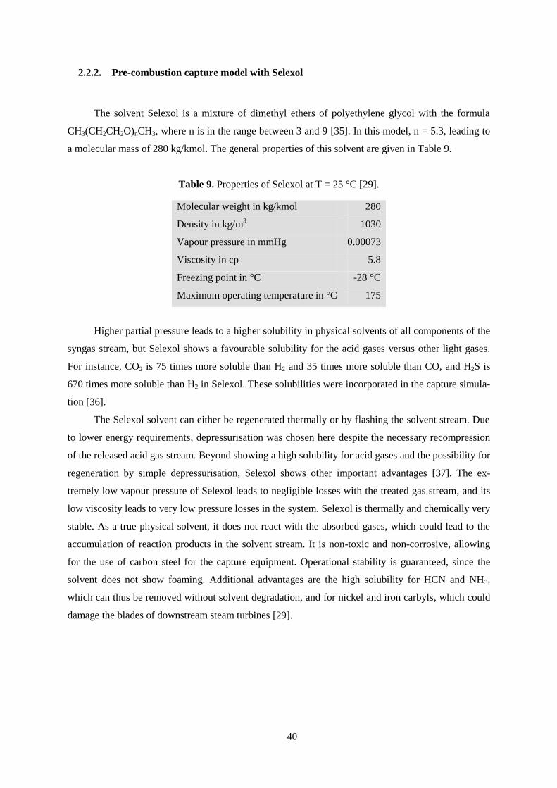
40
2.2.2. Pre-combustion capture model with Selexol
The solvent Selexol is a mixture of dimethyl ethers of polyethylene glycol with the formula
CH3(CH2CH2O)nCH3, where n is in the range between 3 and 9 [35]. In this model, n = 5.3, leading to
a molecular mass of 280 kg/kmol. The general properties of this solvent are given in Table 9.
Table 9. Properties of Selexol at T = 25 °C [29].
Molecular weight in kg/kmol 280
Density in kg/m3 1030
Vapour pressure in mmHg 0.00073
Viscosity in cp 5.8
Freezing point in °C -28 °C
Maximum operating temperature in °C 175
Higher partial pressure leads to a higher solubility in physical solvents of all components of the
syngas stream, but Selexol shows a favourable solubility for the acid gases versus other light gases.
For instance, CO2 is 75 times more soluble than H2 and 35 times more soluble than CO, and H2S is
670 times more soluble than H2 in Selexol. These solubilities were incorporated in the capture simula-
tion [36].
The Selexol solvent can either be regenerated thermally or by flashing the solvent stream. Due
to lower energy requirements, depressurisation was chosen here despite the necessary recompression
of the released acid gas stream. Beyond showing a high solubility for acid gases and the possibility for
regeneration by simple depressurisation, Selexol shows other important advantages [37]. The ex-
tremely low vapour pressure of Selexol leads to negligible losses with the treated gas stream, and its
low viscosity leads to very low pressure losses in the system. Selexol is thermally and chemically very
stable. As a true physical solvent, it does not react with the absorbed gases, which could lead to the
accumulation of reaction products in the solvent stream. It is non-toxic and non-corrosive, allowing
for the use of carbon steel for the capture equipment. Operational stability is guaranteed, since the
solvent does not show foaming. Additional advantages are the high solubility for HCN and NH3,
which can thus be removed without solvent degradation, and for nickel and iron carbyls, which could
damage the blades of downstream steam turbines [29].
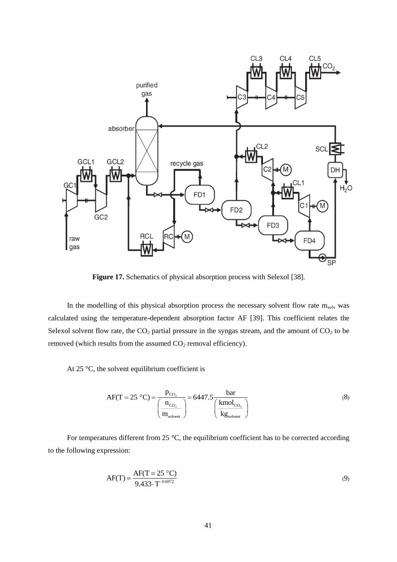
41
Figure 17. Schematics of physical absorption process with Selexol [38].
In the modelling of this physical absorption process the necessary solvent flow rate msolv was
calculated using the temperature-dependent absorption factor AF [39]. This coefficient relates the
Selexol solvent flow rate, the CO2 partial pressure in the syngas stream, and the amount of CO2 to be
removed (which results from the assumed CO2 removal efficiency).
At 25 °C, the solvent equilibrium coefficient is
2
2 2
CO
CO CO
solvent solvent
p barAF(T 25 C) 6447.5
n kmol
m kg
(8)
For temperatures different from 25 °C, the equilibrium coefficient has to be corrected according
to the following expression:
0.6972
AF(T 25 C)AF(T)
9.433 T
(9)

42
The CO2-rich solvent is depressurised after the absorber to a pressure slightly lower than the
solvent equilibrium pressure in order to release the absorbed CO and H2 in a flash drum. Since also
part of the captured CO2 gets released, the gas leaving the flash drum gets repressurised and cooled,
after which it enters the absorber again together with the syngas from the shift section. Recycle gas
flow rate and composition strongly depend on the pressure in the first drum. The solvent gets nearly
completely stripped of the absorbed CO2 by further depressurisation in additional flash drums (at 4
bar, 2 bar and 1 bar). From there the released CO2 is sent to an intercooled compressor for liquefaction
and transport. The lean solvent is then recycled and cooled down to the desired absorber temperature
again. At T = 30 °C and an absorber pressure of 18 bar the following linear relationship between sol-
vent mass flow and removed CO2 was found to be valid for solvent flows of 500 kg/s to 700 kg/s:
mCO2,rem = 0.029 · msolv - 0.159 (10)
This means that the necessary solvent flow for 90% CO2 capture was 660 kg/s. For H2S, a cap-
ture rate of 99.9% resulted. The solubilities and the necessary solvent mass flow were calculated in
FORTRAN calculator blocks, which determined the component flows leaving the top and the bottom
of the absorber and the flash drums. In order to be able to control these flows with the calculator
blocks, the above mentioned system components were modelled with SEP2 columns.

43
2.2.3. Simulations of pre-combustion co-capture with MDEA
MDEA is a so called hindered tertiary amine. This means that CO2 first has to dissolve into the
solvent before it reacts with it [40]. The high syngas pressure facilitates this dissolution, however, so
that in the case of pre-combustion capture, MDEA is a feasible option [41]. Being a chemical solvent,
MDEA requires a significant amount of energy in the form of heat for its regeneration in order to
break the chemical bonds with the captured CO2. Usually steam is extracted from the steam turbine
system to supply this heat. Due to their weaker chemical links, however, the energy requirements for
tertiary amines are lower than for the regeneration of primary amines such as MEA. Generally,
chemical solvents require less solvent circulation and thus less plant investment costs than physical
solvents. As a compromise between necessary investment costs and high energy penalty, MDEA is
also often applied in a mixed solvent processes, such as the Sulfinol process by Shell [42]. The mo-
lecular structure and other parameters of MDEA are shown in Table 10.
Table 10. Properties of MDEA at T = 20 °C [29, 43].
Molecular structure NHO OH
Molecular formula CH3N(C2H4OH)2
Molecular weight in kg/kmol 119.163
Density in kg/m3 1043
Vapour pressure in mmHg < 0.01
Viscosity in cp 101
Freezing point in °C -21 °C
Boiling point in °C 247
Due to the presence of ionic species, the electrolyte NRTL activity coefficient model is used for
the liquid phase and the Redlich-Kwong equation of state for the vapour phase. The phase equilibrium
model was regressed to VLE data from Jou et al. [44, 45, 46].
H2S and CO2 in aqueous solutions react in an acid-base buffer mechanism with alkanolamines.
These equilibrium reactions can be written as chemical dissociation:
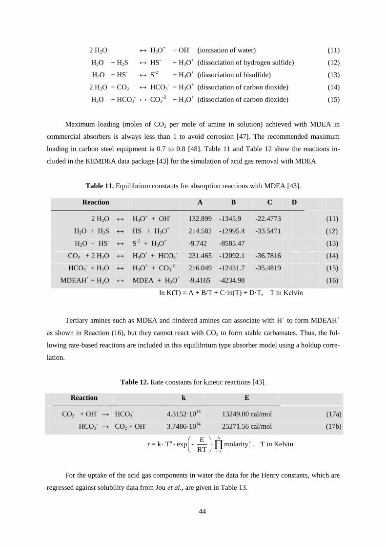
44
2 H2O ↔ H3O+ + OH
- (ionisation of water) (11)
H2O + H2S ↔ HS- + H3O
+ (dissociation of hydrogen sulfide) (12)
H2O + HS- ↔ S
-2 + H3O
+ (dissociation of bisulfide) (13)
2 H2O + CO2 ↔ HCO3-
+ H3O+ (dissociation of carbon dioxide) (14)
H2O + HCO3- ↔ CO3
-2 + H3O
+ (dissociation of carbon dioxide) (15)
Maximum loading (moles of CO2 per mole of amine in solution) achieved with MDEA in
commercial absorbers is always less than 1 to avoid corrosion [47]. The recommended maximum
loading in carbon steel equipment is 0.7 to 0.8 [48]. Table 11 and Table 12 show the reactions in-
cluded in the KEMDEA data package [43] for the simulation of acid gas removal with MDEA.
Table 11. Equilibrium constants for absorption reactions with MDEA [43].
Reaction A B C D
2 H2O ↔ H3O+ + OH
- 132.899 -1345.9 -22.4773 (11)
H2O + H2S ↔ HS- + H3O
+ 214.582 -12995.4 -33.5471 (12)
H2O + HS- ↔ S
-2 + H3O
+ -9.742 -8585.47
(13)
CO2 + 2 H2O ↔ H3O+
+ HCO3- 231.465 -12092.1 -36.7816 (14)
HCO3- + H2O ↔ H3O
+ + CO3
-2 216.049 -12431.7 -35.4819 (15)
MDEAH+ + H2O ↔ MDEA + H3O
+ -9.4165 -4234.98 (16)
ln K(T) = A + B/T + C·ln(T) + D·T, T in Kelvin
Tertiary amines such as MDEA and hindered amines can associate with H+ to form MDEAH
+
as shown in Reaction (16), but they cannot react with CO2 to form stable carbamates. Thus, the fol-
lowing rate-based reactions are included in this equilibrium type absorber model using a holdup corre-
lation.
Table 12. Rate constants for kinetic reactions [43].
Reaction k E
CO2 + OH
- → HCO3
- 4.3152·10
13 13249.00 cal/mol (17a)
HCO3- → CO2 + OH
- 3.7486·10
14 25271.56 cal/mol (17b)
i
Nan
i
i=1
Er = k T exp - molarity , T in Kelvin
RT
For the uptake of the acid gas components in water the data for the Henry constants, which are
regressed against solubility data from Jou et al., are given in Table 13.

45
Table 13. Henry constants of acid gas components in water [43].
i j aij bij cij dij Tlower in K Tupper in K
CO2 H2O 170.7126 -8477.711 -21.9574 0.005781 273 500 (18)
H2S H2O 358.138 -13236.8 -55.0551 0.059565 273 423 (19)
ln Hij = A + B/T + C·ln(T) + D·T, T in Kelvin, Hij in N/m2
The basic configuration used for the simulations consists of a 6 stage absorber column (height 8 m,
diameter 3.75 m) and a two-stage desorber column (height 4 m, diameter 4.95 m), both equipped with
sieve trays.
In the simulations solutions of 50 %wt. MDEA were used. At atmospheric pressure, MDEA is
easily regenerated to a near 100% at a temperature of around 103 °C, so that further heating has no
effect on CO2 capture performance. Keeping the reboiler temperature at 102 °C and elevating the
solvent flow from 100 kg/s to 170 kg/s, reaching 97.8% removal efficiency, the amount of captured
CO2 increased with 0.109 kg per kg of solvent. Maintaining the stripper temperature requires 300 kW
for every kg of solvent added. Since a higher solvent flow has a strong effect on equipment size and
cost and also requires more heating to reach a given reboiler temperature, a balance between solvent
flow and reboiler duty has to be found in order to achieve the desired capture efficiency.
The concentrations of absorbed carbon dioxide and hydrogen sulfide in the liquid phase along
the absorber are shown in Figure 18 for the rich solvent loading of 0.8.
Figure 18. Acid gas concentrations in absorber with MDEA at a rich loading of 0.8.
As can be seen, in the equilibrium model CO2 was absorbed almost up to maximum loading in
the first two stages of the absorber. Thereafter, almost no change was observed. H2S got continuously
absorbed along the absorber.
1
2
3
4
5
6
0 0.1 0.2 0.3 0.4
stage
nu
mb
er
CO2 concentration (kmol/kmol)
1
2
3
4
5
6
0 0.001 0.002 0.003 0.004 0.005
stage
nu
mb
er
H2S concentration (kmol/kmol)
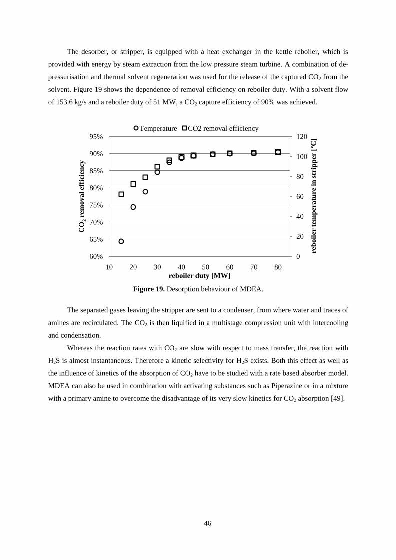
46
The desorber, or stripper, is equipped with a heat exchanger in the kettle reboiler, which is
provided with energy by steam extraction from the low pressure steam turbine. A combination of de-
pressurisation and thermal solvent regeneration was used for the release of the captured CO2 from the
solvent. Figure 19 shows the dependence of removal efficiency on reboiler duty. With a solvent flow
of 153.6 kg/s and a reboiler duty of 51 MW, a CO2 capture efficiency of 90% was achieved.
Figure 19. Desorption behaviour of MDEA.
The separated gases leaving the stripper are sent to a condenser, from where water and traces of
amines are recirculated. The CO2 is then liquified in a multistage compression unit with intercooling
and condensation.
Whereas the reaction rates with CO2 are slow with respect to mass transfer, the reaction with
H2S is almost instantaneous. Therefore a kinetic selectivity for H2S exists. Both this effect as well as
the influence of kinetics of the absorption of CO2 have to be studied with a rate based absorber model.
MDEA can also be used in combination with activating substances such as Piperazine or in a mixture
with a primary amine to overcome the disadvantage of its very slow kinetics for CO2 absorption [49].
0
20
40
60
80
100
120
60%
65%
70%
75%
80%
85%
90%
95%
10 20 30 40 50 60 70 80
reb
oil
er t
emp
era
ture
in
str
ipp
er [°C
]
CO
2re
mo
va
l ef
fici
ency
reboiler duty [MW]
Temperature CO2 removal efficiency

47
2.2.4. Influence of pre-combustion capture on IGCC performance
For the calculation of the overall process efficiency, the influence of water-gas-shift reaction
and acid gas capture on the heating value of the fuel gas streams for the combustion turbine are of
great importance. The compositions and heating values of the key streams as obtained from the IGCC
model are listed in Table 14.
Table 14. Compositions and heating values of gas streams in IGCC with acid gas capture.
Raw
syngas
Shifted
syngas
MDEA Selexol
Sweet gas CO2 stream Sweet gas CO2 stream
Temperature in °C 141 30 78.4 25 29.6 25
Pressure in bar 19 19 19 110 18 110
Mass Flow in kg/s 18.65 24.234 4.673 19.398 3.961 20.209
LHV in MJ/kg 9.8 6.8 35.2 -- 39.4 --
Enthalpy flow in MW 182.1 164.8 164.6 -- 156.0 --
Mole fractions
H2O 0.111 0.003 0.020 -- 10 ppm --
CO2 0.072 0.420 0.067 0.976 0.071 0.938
N2 0.004 0.003 0.005 -- 0.005 37 ppm
CO 0.449 0.024 0.038 -- 0.022 0.027
H2S 0.011 0.009 0.001 0.024 1 ppm 0.022
H2 0.213 0.541 0.868 -- 0.902 0.013
The outlet stream from the low pressure steam turbine is directed through the kettle reboiler of
the stripper, where it condenses and heats the solvent. The outlet pressure of the steam turbine de-
pends on the heat duty requirement of the reboiler and the allowed minimum temperature difference
there. At an assumed minimum temperature difference of 13 °C, the outlet pressure was 1.8 bar for
the stripping of 153.6 kg/s loaded MDEA solution.
In Table 15, the cycle and the removal efficiencies of the different removal options are com-
pared to direct firing of the gasified coal stream without capture. Here, steam extractions for shift sec-
tion, reboiler duty, and power consumption for CO2 compression and for driving the gas and solvent
streams inside the absorption units are included. All compressors have an isentropic efficiency of
86%, while turbines have an isentropic efficiency of 90%.
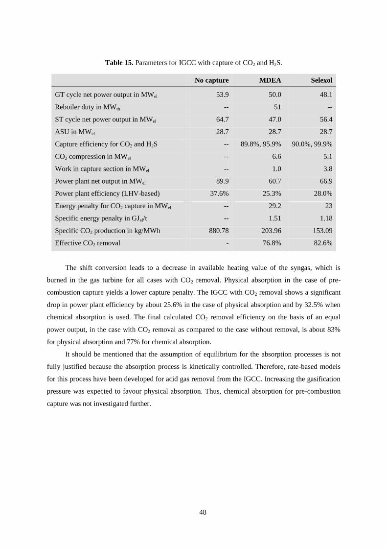
48
Table 15. Parameters for IGCC with capture of CO2 and H2S.
No capture MDEA Selexol
GT cycle net power output in MWel 53.9 50.0 48.1
Reboiler duty in MWth -- 51 --
ST cycle net power output in MWel 64.7 47.0 56.4
ASU in MWel 28.7 28.7 28.7
Capture efficiency for CO2 and H2S -- 89.8%, 95.9% 90.0%, 99.9%
CO2 compression in MWel -- 6.6 5.1
Work in capture section in MWel -- 1.0 3.8
Power plant net output in MWel 89.9 60.7 66.9
Power plant efficiency (LHV-based) 37.6% 25.3% 28.0%
Energy penalty for CO2 capture in MWel -- 29.2 23
Specific energy penalty in GJel/t -- 1.51 1.18
Specific CO2 production in kg/MWh 880.78 203.96 153.09
Effective CO2 removal - 76.8% 82.6%
The shift conversion leads to a decrease in available heating value of the syngas, which is
burned in the gas turbine for all cases with CO2 removal. Physical absorption in the case of pre-
combustion capture yields a lower capture penalty. The IGCC with CO2 removal shows a significant
drop in power plant efficiency by about 25.6% in the case of physical absorption and by 32.5% when
chemical absorption is used. The final calculated CO2 removal efficiency on the basis of an equal
power output, in the case with CO2 removal as compared to the case without removal, is about 83%
for physical absorption and 77% for chemical absorption.
It should be mentioned that the assumption of equilibrium for the absorption processes is not
fully justified because the absorption process is kinetically controlled. Therefore, rate-based models
for this process have been developed for acid gas removal from the IGCC. Increasing the gasification
pressure was expected to favour physical absorption. Thus, chemical absorption for pre-combustion
capture was not investigated further.

49
2.3. Rate-based pre-combustion capture models
In order to achieve more realistic results for capture performance and equipment size, the kine-
tics of absorption has to be taken into account. This is done in the following. The acid gas components
are removed from the shifted syngas by physical absorption with Selexol. One configuration captures
H2S and CO2 separately, while the other one is used for co-capture of these gases.
2.3.1. IGCC for rate-based pre-combustion capture models
A 500 MW Internal Gasification Combined Cycle power plant with four pressure levels in the
steam cycle was the basis for this study on pre-combustion CO2 capture [50]. The plant uses an air
separation unit to provide oxygen for the slurry-fed Texaco gasifier. As recommended for combustion
processes, all blocks in this section were modelled using the Peng-Robinson equation of state.
Figure 20. Process flowsheet of IGCC with acid gas removal [50].
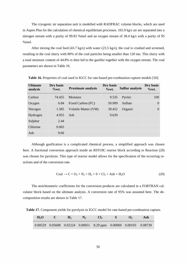
50
The cryogenic air separation unit is modelled with RADFRAC column blocks, which are used
in Aspen Plus for the calculation of chemical equilibrium processes. 165.9 kg/s air are separated into a
nitrogen stream with a purity of 99.83 %mol and an oxygen stream of 38.4 kg/s with a purity of 95
%mol.
After mixing the coal feed (43.7 kg/s) with water (23.5 kg/s), the coal is crushed and screened,
resulting in the coal slurry with 80% of the coal particles being smaller than 120 mu. This slurry with
a total moisture content of 44.8% is then led to the gasifier together with the oxygen stream. The coal
parameters are shown in Table 16.
Table 16. Properties of coal used in IGCC for rate-based pre-combustion capture models [50].
Ultimate
analysis
Dry basis Proximate analysis
Dry basis Sulfur analysis
Dry basis
%wt. %wt. %wt.
Carbon 74.455 Moisture 9.535 Pyritic 100
Oxygen 6.84 Fixed Carbon (FC) 50.909 Sulfate 0
Nitrogen 1.585 Volatile Matter (VM) 39.452 Organic 0
Hydrogen 4.955 Ash 9.639
Sulphur 2.44
Chlorine 0.065
Ash 9.66
Although gasification is a complicated chemical process, a simplified approach was chosen
here. A fractional conversion approach inside an RSTOIC reactor block according to Reaction (20)
was chosen for pyrolysis. This type of reactor model allows for the specification of the occurring re-
actions and of the conversion rate.
Coal → C + O2 + N2 + H2 + S + Cl2 + Ash + H2O (20)
The stoichiometric coefficients for the conversion products are calculated in a FORTRAN cal-
culator block based on the ultimate analysis. A conversion rate of 95% was assumed here. The de-
composition results are shown in Table 17.
Table 17. Component yields for pyrolysis in IGCC model for rate-based pre-combustion capture.
H2O C H2 N2 Cl2 S O2 Ash
0.00529 0.05608 0.02224 0.00051 8.29 ppm 0.00069 0.00193 0.08739

51
The gasification reactions are not specified further. An equilibrium approach in an RGIBBS re-
actor block was chosen for this process. This approach considers all specified components as possible
products and calculates equilibrium by minimisation of Gibbs free energy. The main parameters cho-
sen for the IGCC are shown in Table 18. They agree well with realistic values.
Table 18. IGCC operation parameters.
Gasification temperature in °C 1455
Gasification pressure in bar 44
Combustion temperature in °C 1350
Coal flow rate in kg/s 34.7
Oxygen/Coal mass ratio 0.88
Steam pressure levels in bar 161.9, 40.6, 7.3, 3.1, 0.068
HP steam turbine inlet temperature in °C 563
After the gasification, impurities such as ash, unreacted coal, and nitrides are removed from the
gas streams by a filter or cyclone, here modelled with a SEP block. This block allows for the specifi-
cation of the solid components that leave the process. Denitrification was achieved by grey water
wash (water and NH3) in a FLASH2 block according to the following reactions:
Table 19. Equilibrium constants for grey water wash [50].
Reaction A B C D
2 H2O ↔ H3O+ + OH
- 132.899 -1345.9 -22.4773 (11)
H2O + H2S ↔ HS- + H3O
+ 214.582 -12995.4 -33.5471 (12)
H2O + HS- ↔ S
-2 + H3O
+ -9.742 -8585.47
(13)
H2O + NH3 ↔ NH4+ + OH
- -1.257 -3335.7 1.4971 -0.0371 (21)
2 H2O + SO2 ↔ H3O+ + Cl
- -5.979 637.396
-0.0151 (22)
H2O + HSO3- ↔ H3O
+ + SO3
-2 -25.291 1333.4
(23)
2 H2O + CL2 ↔ H3O+ + Cl
- + HClO -11.375 -1286.972
(24)
H2O + HClO ↔ H3O+ + ClO
- -16.152 -1602.87
(25)
NH4Cl SALT NH4
+ + Cl
- -141.676 -880.103 27.7806 -0.0632 (26)
(NH4)2SO3 SALT 2 NH4
+ + SO3
-2 920.378 -44503.83 -139.3449 0.0362 (27)
((NH4)2SO3)aq SALT
2 NH4+ + SO3
-2 + H2O -1297.041 33465.89 224.2223 -0.3516 (28)
NH4HS SALT NH4
+ + HS
- minimisation of Gibbs free energy (29)
NH4HSO3 SALT NH4
+ + HSO3
- minimisation of Gibbs free energy (30)
ln K(T) = A + B/T + C·ln(T) + D·T, T in Kelvin

52
The pre-treated gas stream is then sent to COS hydrolysis, which is modelled with another
RSTOIC reactor, showing a fractional conversion of 90% of the COS in the gas stream according to
Reaction (31).
COS + H2O → CO2 + H2S (31)
After passing the COS hydrolysis reactor, the gas stream enters the intercooled two-stage sour
water-gas-shift section with reactor temperatures of 700 °C and 400 °C. With a necessary steam flow
of 32.5 kg/s 98% of the CO content is converted.
Afterwards, H2S and CO2 are removed in the capture section, while the remaining H2-rich gas
stream is burned in a gas turbine. The gas turbine exhaust gases are used to produce steam for electric-
ity generation in steam turbines.

53
2.3.2. Rate-based separate pre-combustion capture of CO2 and H2S with Selexol
In this study the author investigated two capture configurations with Selexol, either for simulta-
neous or for separate capture of H2S and CO2. The first configuration captures H2S and CO2 sepa-
rately. For this purpose, the H2S absorber as presented in Figure 21 uses Selexol preloaded with CO2
coming from the CO2 absorber. In order to improve the selectivity of the H2S absorber, gas from the
solvent regeneration of the CO2 section is mixed to the cooled syngas stream coming from the water-
gas-shift reactors. H2S is separated from the solvent stream in a stripper column. The energy for the
solvent regeneration is provided by steam extraction from the combined cycle, reducing power plant
efficiency [51].
H2S
stripper
Lean-rich
heat exchanger
H2S
absorber
Solvent
flash
Syngas
cooler
Syngas
Preloaded solvent
from CO2 absorber
and makeup
Flash gas from
CO2 solvent regeneration
Lean solvent to CO2 absorber
H2S solvent
concentratorH2S free gas to CO2 absorber
Acid gas
Figure 21. Pre-combustion H2S capture section with Selexol (after [52]).
The H2S-free syngas leaving the H2S absorber is then directed to the CO2 absorber as shown in
Figure 22. The same applies to the regenerated lean solvent from the H2S capture section.
The layout shown here is based on the UOP Selexol process as reported by Breckendridge [52].

54
In the CO2 capture section, regeneration of the solvent is achieved by depressurisation in flash
drums (FD). The CO2 released in flash drums 3 and 4 is then compressed for mixing with the CO2
leaving FD2. After water condensation, the CO2 stream is then compressed for transport and storage.
CO2
absorberIntercooled CO2 compression
Partially treated
syngas from
H2S absorber
Treated gasLean solvent from
H2S regeneration
and makeup
FD2
FD1
FD3
FD4
Flash gas
to H2S absorber
CO2 saturated
Solvent
to H2S absorber
Figure 22. Pre-combustion CO2 capture section with Selexol (after [52]).
All columns are modelled with RATESEP blocks, which are used in Aspen Plus for the simula-
tion of rate-based processes. For modelling the absorption of acid gas components into the Selexol
solvent, the PC-SAFT equation of state was applied [53]. This EOS is used to describe VLE in poly-
mer solvents over a wide range of temperatures and pressures [54, 55, 56].
With this model , a sufficiently high concentration of H2S in the acid gas stream leaving the
H2S stripper column could not be achieved here. Higher values would make its use in a Claus process
for the production of sulphur attractive. Different researchers [29, 52] claim to achieve an H2S con-
centration of more than 45% in this process.

55
The maximum height of the columns with the Flexipac 1Y packing in this process was assumed
to be 20m. The diameter was calculated for a maximum flooding of 80% for a stable operation. The
key parameters obtained from the model are summarised for both capture sections in Table 20. The
model was set to achieve an acid gas removal as reported in Table 24, where the performance of this
model is compared to a second model, which was used for the co-capture of H2S and CO2.
Table 20. Key parameters of rate-based H2S capture and CO2 capture sections with Selexol.
H2S capture section
Preloaded solvent flow, CO2 loading, H2S loading 471 kg/s, 1.13 mol/mol, 0.0056 mol/mol
Gas inlet and solvent temperature 24.1 °C, 25 °C
H2S rich loading 0.03 mol/mol
H2S lean loading after stripper 0.0098 mol/mol
Column packing and design parameter for diameter Flexipac 1Y, 80% flooding
Pressure, height and diameter of packed absorber column 41.5 bar, 20 m, 6 m
Pressure, height and diameter of packed stripper column 4 bar, 3 m, 2.1 m
Reboiler duty (MW) and temperature 20 MWth, 113 °C
Solvent concentrator pressure, solvent flash pressure 43 bar, 8 bar
Solvent makeup 0.005 kg/s
CO2 capture section
Solvent flow from H2S regeneration, CO2 loading 403 kg/s, 0.0336 mol/mol
Solvent flow from CO2 regeneration, CO2 loading 1513 kg/s, 0.0525 mol/mol
Gas inlet and solvent temperature 25.3 °C, -1.1 °C
Column packing and design parameter for diameter Flexipac 1Y, 80% flooding
Pressure, height and diameter of packed absorber column 41 bar, 20 m, 8.4 m
Flash drum pressures (FD1 - 4) 8 bar, 4 bar, 2 bar, 1 bar
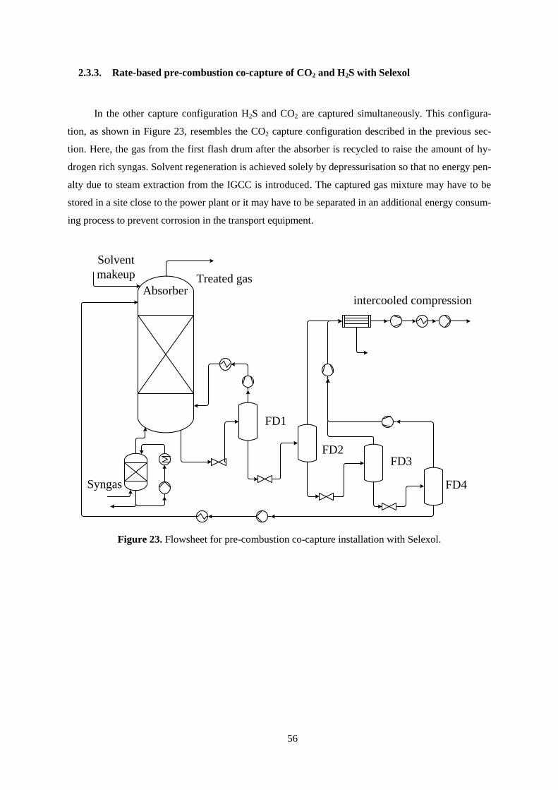
56
2.3.3. Rate-based pre-combustion co-capture of CO2 and H2S with Selexol
In the other capture configuration H2S and CO2 are captured simultaneously. This configura-
tion, as shown in Figure 23, resembles the CO2 capture configuration described in the previous sec-
tion. Here, the gas from the first flash drum after the absorber is recycled to raise the amount of hy-
drogen rich syngas. Solvent regeneration is achieved solely by depressurisation so that no energy pen-
alty due to steam extraction from the IGCC is introduced. The captured gas mixture may have to be
stored in a site close to the power plant or it may have to be separated in an additional energy consum-
ing process to prevent corrosion in the transport equipment.
Absorberintercooled compression
Treated gas
Solvent
makeup
FD2
FD1
FD3
FD4Syngas
Figure 23. Flowsheet for pre-combustion co-capture installation with Selexol.

57
Compared to the model for separate acid gas removal, solvent flow and column height could be
reduced for a CO2 capture efficiency of 90%. The key parameters for this capture option can be found
in Table 21. The pressure of flash drum 1 has a major influence on the performance of the capture
process. Since the gas stream leaving this component needs to be recompressed before recycling to
the absorber column, higher pressures lead to lower energy consumption in the recycle compressor.
Lower pressures lead to a higher hydrogen flow in the purified gas stream and thus to a higher energy
content of this fuel gas stream that is the burned in the gas turbine. The pressures of the other flash
drums were selected to allow for the more economical use of identical compressors due to equal pres-
sure ratios.
Table 21. Key parameters of rate-based co-capture section with Selexol.
Solvent flow 825 kg/s
Lean loading, rich loading for CO2 0.0496 mol/mol, 0.7141 mol/mol
Lean loading, rich loading for H2S 0.0051 mol/mol, 0.0082 mol/mol
Gas inlet and solvent temperature 32.5 °C, -1.1 °C
Column packing and design parameter for diameter Flexipac 1Y, 80% flooding
Pressure, height and diameter of packed absorber column 41 bar, 11 m, 5.3 m
Flash drum pressures (FD1 - 4) 18 bar, 5 bar, 2.25 bar, 1 bar
The compositions and flows of the syngas streams and of the streams leaving the capture sec-
tions are listed in Table 22. As was to be expected, the purity of the purified gas stream and that of the
CO2 stream are higher in the case of separate acid gas removal. However, only an H2S concentration
of 4.5% was achieved there for the H2S-rich stream.
Table 22. Composition and flow of gas streams.
separate capture co-capture
syngas shifted purified H2S rich CO2 stream purified acid gas
Mass Flow in kg/sec 88.54 118.40 14.95 3.93 92.23 24.14 114.68
Mole Fractions
CO 0.436 0.002 0.004 0.000 0.000 0.004 0.000
CO2 0.125 0.397 0.040 0.953 0.996 0.070 0.990
H2 0.286 0.512 0.923 0.000 0.000 0.896 0.004
H2O 0.130 0.072 0.000 0.002 0.000 0.000 0.000
N2 0.009 0.007 0.032 0.000 0.001 0.030 0.001
H2S 0.003 0.002 518 ppm 0.045 0.003 262 ppm 0.005

58
As reported in Table 24, shifting the syngas leads to a slight drop in power plant efficiency and
would not make sense without capture of the acid gas components. The flue gas parameters of the
IGCC with and without pre-combustion capture is reported in Table 23.
Table 23. Composition and flow of burned gas streams.
no shift, no capture separate capture co-capture
Mass Flow in kg/sec 694.44 656.62 644.94
Mole Fractions
N2 0.688 0.721 0.717
O2 0.121 0.131 0.128
Ar 0.011 0.009 0.009
H2O 0.082 0.133 0.135
CO2 0.098 0.006 0.010
SO2 463 ppm 69 ppm 37 ppm
HCl trace -- --
As can be seen from these data, the CO2 and SO2 contents in the flue gas stream is significantly
reduced due to pre-combustion capture. The capture efficiencies of the two investigated options are
reported in Table 24.

59
2.3.4. Influence of pre-combustion capture (rate-based models) on IGCC performance
The use of the different capture configurations led to different impacts on the power plant,
mainly due to the difference in the energy requirements for solvent regeneration. Calculated values for
the main parameters are presented in Table 24.
The theoretical advantage of separate capture, i.e. a concentrated acid gas stream for production
of elementary sulphur in a Claus plant could not be achieved in the simulations, as the H2S concentra-
tions yielded were too low. Therefore, the recommended option here is co-capture of H2S and CO2,
possibly with later separation of these gases in another process.
Table 24. Parameters for IGCC with and without pre-combustion capture of CO2 and H2S.
shift
no capture
no shift,
no capture
separate
capture co-capture
Power plant output in MWel 573.75 576.25 561.25 567.5
ASU in MWel 120 120 120 120
Capture efficiency for CO2 and H2S -- -- 94.4%, 84.7% 90.0%, 91.9%
CO2 compression in MWel -- -- 16.25 23.75
Solvent chilling in MWel (COP = 4.5) -- -- 10.01 1.88
Work in H2S capture section -- -- 9.98 --
Work in CO2 capture section -- -- 12.53 8.75
Power plant net output in MWel 453.8 456.3 392.5 412.5
Power plant efficiency (HHV-based) 38.40% 38.60% 33.20% 34.90%
Energy penalty for capture in MWel -- -- 63.75 43.75
Specific energy penalty in GJel/t -- -- 0.67 0.48
Specific CO2 production in kg/MWh 647.7 644.1 78.1 74.4
Effective CO2 removal -- -- 87.9% 88.5%
In the simulations studied here, separate capture of the acid gas components led to a lower cap-
ture efficiency for H2S, even though the CO2 capture rate was raised above 90%. This also led to a
higher energy penalty for the capture process. The high necessary solvent flow required more energy
for solvent cooling and pumping, as well as for the recompression of the gas streams. Raising CO2
capture efficiency to the reported level was necessary to achieve a similar effective CO2 capture effi-
ciency as with the co-capture option [51].

60
3. Post-combustion capture
Most anthropogenic point sources of CO2 are combustion systems such as power plants, cement
kilns and furnaces as used for iron and steel production, where the fuel is burned with air. Post-
combustion capture is the removal of greenhouse gases at the end of the conversion process. There-
fore, this second capture method discussed in the following is a very important process for reducing
CO2 emissions. Since these combustion processes are of large scale, occur at low pressure and due to
the large nitrogen content of air, they produce very large gas flows with a low content of CO2. This
content ranges from 3 %vol. for a NGCC to about 15% for a coal-fired power plant. Due to the low
partial pressure of CO2 in the gas stream, liquid separation is a possible candidate. However, the de-
velopment of ceramic or metallic membranes would possibly yield more efficient solutions of CO2
separation [57, 58]. Another approach is the use of liquid membranes that combine chemical solvents
with membranes [59, 60, 61]. Other capture technologies are pressure swing adsorption on molecular
sieves and cryogenic gas separation. Of these approaches, this chapter will focus on the use of chemi-
cal solvents for post-combustion CO2 capture. Chemical solvent absorption is currently the most
promising and cost-effective technology [30].
Impurities such as SOX, NOX, particulates, HCl, HF, metals (mercury etc.) and other contami-
nants may negatively affect capture performance by causing solvent degradation. Especially the most
widely used solvent monoethanolamine (MEA) is prone to degradation [62], which is caused by oxy-
gen and oxygen-containing components such as NOX and SOX, by producing oxidised amine frag-
ments, NH3, formate, acetate and peroxides [63, 64]. Degradation can be catalysed by metal cations
present in the absorption section [65]. Iron is often present due to corrosion, which is especially pro-
nounced in carbon steel equipment. Corrosion is mainly influenced by CO2 loading of the solvent and
by the solvent type [66], but also by the presence of degradation products, and by temperature and
solvent concentration [65]. Corrosion inhibitors such as carboxylic acids act as oxygen scavengers
and can significantly reduce steel corrosion in the capture plant [67]. In the presence of oxygen, SO2
dissolved in MEA reacts very quickly to form heat stable sulphates that have to be removed to main-
tain solvent performance [64]. NOX are easily dissolved in water forming corrosive acids, and like
SO2 they can react irreversibly with alkanolamines [68, 69], causing a continuous loss of solvent [30].
Therefore, these components have to be removed to very low levels in the flue gas prior to entering
the absorption section [65]. In Figure 24, a schematic diagram of a PC power plant with emission con-
trols is shown.

61
Figure 24. Pulverised coal power plant with amine CO2 capture and other emission controls [12].
Chemical CO2 absorption makes use of the reaction of a weak alkanolamines base with CO2,
which is a weak acid, to form a water-soluble salt [65]. This reversible and temperature dependent
reaction can be written in simplified form as:
cold
2 2 3hot
CO 2RNH RNHCOO RNH
(32)
The carbamate ion RNHCOO- can be formed by primary ions such as MEA and by secondary
amines. From this reaction it can be seen that two moles of amine are necessary to remove one mole
of CO2. Tertiary amines such as MDEA do not form carbamate ions due to the lack of a hydrogen ion
attached to the nitrogen. Then a different reaction forming bicarbonate ions takes place, which is cata-
lysed by water:
2H O 3
2 3CO R N HCO RNH
(33)
Since only one mole of amine is needed for the removal of one mole of CO2, the absorption ca-
pacity of tertiary and hindered amines is greater. However, their main disadvantage is the much
slower CO2 uptake rate (see 2.2.3). However, absorption kinetics for these solvents can be improved
by adding small quantities of activators such as Piperazine [49]. Also primary amines such as MEA
can be used as activator [70].
Although new amines such as KS-1 with very low degradation are being developed, MEA is
still the most widely used solvent for CO2 capture. It has very high reactivity, low solvent cost, rea-
sonable thermal stability and thermal degradation rate [65].

62
A flow diagram that includes the most important steps of the post-combustion capture process
is shown in Figure 25.
Figure 25. Process flow diagram for CO2 capture by chemical absorption [12].
After passing a blower or fan to compensate for the pressure loss inside the absorber, the flue
gas is cooled and enters the absorber. There, the flue gas comes into contact with the semi-lean sol-
vent. Then a water wash is used to remove any solvent carried over with the scrubbed flue gas. Typi-
cal removal efficiencies are in the range of 80 to 95%. Higher efficiencies lead to taller absorber col-
umns, higher energy penalties and thus to elevated costs. The CO2-rich solvent is then pumped to the
top of a stripper via a heat exchanger to minimise energy penalties. The regeneration of the solvent
occurs at close to atmospheric pressure and at temperatures of 100 °C to 140 °C. The energy require-
ments of the reboiler for the stripper column is composed of the energy for i) bringing the solution to
the boiling point, ii) for breaking the chemical bonds between CO2 and solvent, and iii) for generating
water vapour to establish an operating CO2 partial pressure needed for CO2 stripping [65].
Heat for solvent regeneration is generally supplied by low-pressure steam, leading to the main
energy penalty for CO2 capture. The necessary reboiler duty depends strongly on lean solvent loading
[71, 72, 73]. Being the most influential factor on power plant output, the reboiler duty can be used as a
variable for overall plant efficiency.
In this chapter, capture and power plant performances are compared mainly for chemical ab-
sorption with MEA and with ammonia, since several different studies showed that a significant reduc-
tion of up to 62% in regeneration energy is possible [74, 75]. Alstom is carrying out studies on a pilot

63
plant at the Pleasant Prairie coal-fired power plant by We Energies in Kinosha, WI, USA [76, 77, 78]
and claim that this process uses only about 50% of the energy needed for a comparable MEA process,
leading to an output reduction of only 10% in the power plant. Ammonia can also be used for the si-
multaneous removal of CO2, SO2, and NOX [79]. However, one of the major drawbacks of this proc-
ess is the high loss of ammonia due to its high volatility and the formation of precipitates [80].
In the following, several post-combustion capture models will be developed and discussed.

64
3.1. Equilibrium-based CO2 capture models and experiments
Due to the presence of ionic species in theses multi-component volatile weak electrolyte sys-
tems [17, 18], liquid and vapour properties were computed by the electrolyte NRTL method. Henry’s
law was used to calculate the solubility of CO2 in water. All simulations were carried out with Aspen
Plus, which has become a widely used standard application for computerised flowsheet simulations in
the chemical industry.
3.1.1. PC power plant model
For all post-combustion capture processes the flue gas stream was assumed to exit from a 500
MW pulverised coal power plant with an SCR reactor (RSTOIC) for the removal of NOX with ammo-
nia injection according to Reactions (34) - (36) and wet flue gas desulfurisation according to Reaction
(37) in a RADFRAC column with a conversion factor of 0.26 for CaCO3.
2 NO2 + 4 NH3 + O2 ↔ 3 N2 + 6 H2O (34)
NO + NO2 + 2 NH3 ↔ 2 N2 + 3 H2O (35)
4 NO + 4 NH3 + O2 ↔ 4 N2 + 6 H2O (36)
CaCO3 + SO2 ↔ CaSO3 + CO2 (37)
According to the IEA report on CO2 capture [30], NOX and SOX levels have to be reduced to at
least 20 ppm and 10 ppm respectively to prevent MEA degradation. With ammonia, these contami-
nants can be captured by the solvent. However, they would end up in the separated CO2 stream, where
they may have to be removed to prevent equipment damage due to acid formation. For thermal sol-
vent regeneration in a stripper column steam is extracted after the medium pressure turbines. The pa-
rameters for the IEA coal used in the simulations are shown in Table 25.

65
Table 25. Coal analysis for PC power plant.
Ultimate analysis Dry basis
Proximate analysis Dry basis
Sulphur analysis Dry basis
%wt. %wt. %wt.
Carbon 71.38 Moisture 9.5 Pyritic 0
Oxygen 7.79 Fixed Carbon (FC) 50.51 Sulfate 100
Nitrogen 1.56 Volatile Matter (VM) 36.01 Organic 0
Hydrogen 4.85 Ash 13.48
Sulfur 0.952
Chlorine 0.026
Ash 13.48
The relevant parameters of this typical 3-stage Rankine cycle power plant can be found in Ta-
ble 26. The Peng-Robinson EOS was used for this process, as recommended for the modelling of
combustion processes.
Table 26. PC power plant parameters (after [72]).
Coal Feed 50.4 kg/s
Heating value coal HHV = 27.06 MJ/kg, LHV = 25.87 MJ/kg
HP Turbine pin = 152 bar Tin = 533 °C P = 130.7 MW
IP Turbine pin = 42.5 bar P = 190.1 MW
LP Turbine pin = 4.67 bar P = 243.7 MW
Condenser pcond = 0.04 bar QCooling = 265 MW
Ammonia for SCR 1.436 kg/s
Limestone slurry for FGD 20.548 kg/s (6.74 %wt.), 1.871 kg/s gypsum produced

66
To show the effect of SCR and FGD on the flue gas, the compositions of the treated and of the
untreated flue gas stream are given in Table 27. It is plausible that the water content in the flue gas
increases due to the use of wet FGD.
Table 27. Flue gas composition of PC power plant.
flue gas components composition of untreated flue gas
in %mol
composition with SCR and FGD
in %mol
N2 74.0 70.3
H2O 7.0 12.3
CO2 13.8 13.1
O2 3.5 3.2
CO 0.2 0.2
NOX 0.4 19 ppm
SO2 0.07 9 ppm
The energy penalty involved with the thermal solvent regeneration in a stripper column will be
discussed later.
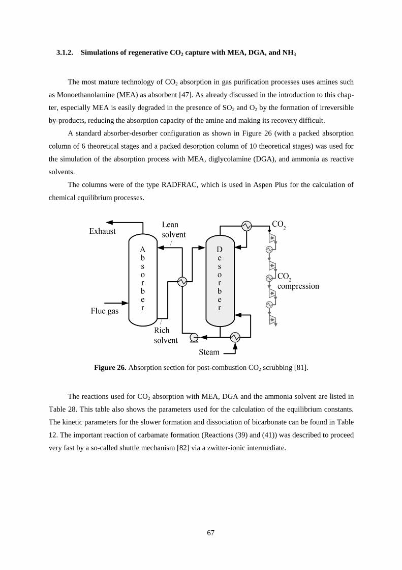
67
3.1.2. Simulations of regenerative CO2 capture with MEA, DGA, and NH3
The most mature technology of CO2 absorption in gas purification processes uses amines such
as Monoethanolamine (MEA) as absorbent [47]. As already discussed in the introduction to this chap-
ter, especially MEA is easily degraded in the presence of SO2 and O2 by the formation of irreversible
by-products, reducing the absorption capacity of the amine and making its recovery difficult.
A standard absorber-desorber configuration as shown in Figure 26 (with a packed absorption
column of 6 theoretical stages and a packed desorption column of 10 theoretical stages) was used for
the simulation of the absorption process with MEA, diglycolamine (DGA), and ammonia as reactive
solvents.
The columns were of the type RADFRAC, which is used in Aspen Plus for the calculation of
chemical equilibrium processes.
Figure 26. Absorption section for post-combustion CO2 scrubbing [81].
The reactions used for CO2 absorption with MEA, DGA and the ammonia solvent are listed in
Table 28. This table also shows the parameters used for the calculation of the equilibrium constants.
The kinetic parameters for the slower formation and dissociation of bicarbonate can be found in Table
12. The important reaction of carbamate formation (Reactions (39) and (41)) was described to proceed
very fast by a so-called shuttle mechanism [82] via a zwitter-ionic intermediate.

68
Table 28. Equilibrium constants for absorption with MEA, DGA, and NH3 [83, 84, 85].
Reaction A B C D
2 H2O ↔ H3O+ + OH
- 132.899 -1345.9 -22.4773 (11)
CO2 + 2 H2O ↔ H3O+
+ HCO3- 231.465 -12092.1 -36.7816 (14)
HCO3- + H2O ↔ H3O
+ + CO3
-2 216.049 -12431.7 -35.4819 (15)
MEAH+ + H2O ↔ MEA + H3O
+ -3.03833 -7008.36
-0.003135 (38)
MEACOO- + H2O ↔ MEA + HCO3
- 231.466 12092.1 36.7816 (39)
DGAH+ + H2O ↔ DGA + H3O
+ -13.3373 -4218.71 (40)
DGACOO- + H2O ↔ DGA + HCO3
- 3.66110 -3696.17 (41)
NH3 + H2O ↔ NH4+ + OH
- -1.257 -3335.7 1.4971 -0.037057 (18)
NH3 + HCO3- ↔ NH2COO
- + H2O -4.583 2900 (42)
NH4HCO3 S A L T
NH4+
+ HCO3- 554.818 -22442.5 -89.0064 0.064732 (43)
(NH4)2CO3 S A L T
2 NH3 + CO2 + H2O by minimisation of Gibbs free energy (44)
NH2COONH4 S A L T
NH4+
+ NH2COO- by minimisation of Gibbs free energy (45)
ln K(T) = A + B/T + C·ln(T) + D·T, T in Kelvin
A comparison of the CO2 removal efficiency per unit mass of solvent is shown in Figure 27.
Ammonia has by far the best absorbent qualities among the substances investigated. For this compari-
son, the solvent flow was held constant for every individual solvent while the solvent concentration
was raised (range of concentrations in % wt.: MEA: 0.17–0.33, DGA: 0.17–0.5, NH3: 0.02–0.2).
Figure 27. CO2 removal eff. at 20 °C of MEA, DGA, and NH3 at different solvent-to-CO2 ratios.
NH3 shows a very high removal efficiency at ambient pressure. For a CO2 removal efficiency
of 80% an ammonia-to-CO2 ratio of ca. 1.5 (a solvent concentration of 7 %wt.) is sufficient, while for

69
the same removal efficiency using MEA an amine-to-CO2 ratio greater than 3 (solvent concentration
of 20 %wt.) is necessary. Solvent concentrations are limited by corrosion and by solvent losses.
Due to the assumption of chemical equilibrium, larger absorption columns of more than 6
stages did not give a significantly higher absorption efficiency in the simulations.

70
3.1.3. CO2 capture simulations with ammonia in a non-regenerative process
The role of ammonia as a promising solvent in CO2 capture is even more enhanced by a novel
method to reduce CO2 emissions from power plants by the use of an aqueous ammonia solution,
which makes it possible to capture CO2 as a valuable solid product [86, 87]. Thus, in this chapter a
special focus is laid on the capture of ammonia salts, as this allows for a much more rational use of
the CO2 than the energy intensive compression and necessary storage of the gaseous carbon dioxide
leaving the absorption process in the case of MEA and DGA. A possible configuration for this capture
option, which was used in the simulations here, is presented in Figure 28. The model configuration
included a packed absorber column of 10 theoretical stages and a filter for the extraction of salt prod-
ucts from the rich solvent leaving the absorber. The lean solvent is recycled to the absorber after in-
serting fresh solvent to make up for the losses attributed to the removal of ammonia salts.
The produced salts are a basic ingredient of fertilizers [88] and could hence be exploited com-
mercially. NH3 has frequently been used as reactant for the De-NOX process in power plants, and it is
also interesting for the removal of SO2 and HCl from flue gases [79].
Figure 28. Schematic diagram of non-regenerative CO2 capture with ammonia.
CO2 scrubbing with ammonia is economically very attractive [81], if salts can be separated,
since the conventional production of the ammonia salts requires an energy input of around 32 GJ/t salt
[89], which is about twice the value for the production of NH3.
As shown in Figure 29, salt formation increases with solvent loading (mol CO2/mol solvent
agent). The salts separated from the solvent stream by filtration or by sedimentation have commercial
appeal for fertilizer production.

71
Figure 29. Ammonia salt formation for different loadings (mol/mol) of the ammonia solvent [90].
Values for the solubility of the ammonia salts are differing between manufacturers. Data sets
for two major manufacturers are given in Table 29.
Table 29. Ammonia salt solubilities [91, 92].
Salts BASF (g/l) Sigma - Aldrich (g/l)
NH4HCO3 178 220
NH4COONH2 423 790
(NH4)2CO3 320 320
In the non-regenerative ammonia process, at 20 °C approximately 20% of the ammonia exits
the absorber with the gas stream and has to be removed.

72
3.1.4. Experiments for CO2 capture with ammonia and EAA solvent
A series of experiments for the investigation of CO2 capture with ammonia solvents was carried
out in a small-scale setup in the laboratory of the Inorganic Chemistry department at the University of
Florence. The semi-continuous flow reactor shown in Figure 30 consisted of a glass column contain-
ing 240 ml of aqueous ammonia solution (5 %wt. ammonia concentration) [87].
Figure 30. Schematic diagram of semi-continuous flow absorber for CO2 [90].
A substitute flue gas stream (10 %vv. CO2 in N2) of ca. 4.2 ml/s was fed continuously to the
bottom of the absorber through a sintered glass diffuser (Ø 16-40 μm pores). The exhaust gas left the
absorber at the top. The inlet gas mixture was humidified by bubbling it through water before it en-
tered the reactor. All experiments were carried out at atmospheric pressure. The CO2 capture perform-
ance of the system is easily determined by weight measurements of all system components before the
tests and after certain time intervals. The pH-value and the species in solution were analysed with a
13C-NMR apparatus. A gas chromatograph was used to measure the losses of CO2 from the system.
Although the reaction between carbonate and bicarbonate reached equilibrium very fast, this
was not the case for the reaction of carbamate with its carbonate and bicarbonate products. Thus, the
solution was given at least 1 h to react, allowing for the measurement of the equilibrium concentra-
tions of bicarbonate, carbonate and carbamate ions. The concentrations of the components in solution
after different time intervals are shown for two different absorption temperatures in

73
Table 30. The loss of ammonia from the absorber in the experiments proved to be very low (ca.
0.01%).

74
Table 30. Development of component concentrations (% wt.) in 5 %wt. ammonia solution [90].
Time (h) T = -5 °C T = 20 °C
HCO3- CO3
-2 NH2COO
- HCO3
- CO3
-2 NH2COO
-
2 28. 1 28.6 43.3 28.2 28.8 43.0
3 42.8 21.9 35.3 45.3 22.7 32.0
7 52.0 18.3 29.7 60.2 16.5 23.3
8 63.3 14.8 21.9 71.0 11.9 17.1
Temperatures of down to -5 °C were investigated, as reduced salt solubility was expected.
However, the CO2 removal efficiency was nearly independent of absorber temperature, as shown in
Figure 31. pH-measurements of the solution verified this behaviour.
Figure 31. CO2 removal efficiency by ammonia solution (5% wt.) at different temperatures [90].
Contrary to the simulation results, the experiments showed that at such low ammonia concen-
trations, it was not possible to separate the salts from the solution. The resulting lower removal effi-
ciency of ammonia in the experiments (ca. 1.26 kgCO2,removed/kgNH3,in), however, is still higher than
that found in the simulation results for MEA and DGA.
In order to separate the ammonia salts it is necessary to lower their solubility. This can be
achieved by either raising the concentration of ammonia in the solvent stream [93, 94] or by using an
alternative solvent. In this work, the latter option was chosen, as otherwise ammonia losses with the
exhaust gas become very large.
Aiming at a reduction of these losses, the hydro-alcoholic solvent EtOH–H2O–NH3 was inves-
tigated [87], resulting in a so-called Ethanol-Aqueous-Ammonia (EAA) solution, consisting of 85
%wt. ethanol and a varying percentage of ammonia, the remaining amount being water. Ethanol was
chosen due to its similar characteristics to water and its good availability. A new series of tests was

75
carried out for various ammonia concentrations and absorber temperatures without changing the de-
scribed experimental setup.
After giving the solution 3 h to react, the CO2 outlet concentration in the gas stream exceeded
20 %wt. for an ammonia concentration of 2 %wt., while it took more than 6 h until the same outlet
concentration of CO2 was observed at ammonia concentrations of 4 %wt. and 6 %wt. Also, the
amount of produced salts confirmed that removal efficiency improved with increasing ammonia con-
centration. At the end of the experiment, when the CO2 outlet concentration exceeded 25 %wt., the
salts are removed from the absorption column. Then, they were dried and weighed to measure their
relative amount, and a sample of the produced salts underwent an NMR analysis to determine the salt
composition. In the end, the absorption column is weighed again and the test is restarted. At an ab-
sorber temperature of 5 °C, about 8.3 g were obtained for a solvent concentration of 2 %wt., while it
were 12.8 g and 13.7 g respectively for solvent concentrations of 4 %wt. and 6 %wt. However, higher
ammonia concentrations in the entering solvent stream also lead to elevated losses of ammonia with
the exiting gas stream.
The results for different absorber temperatures clearly show a reduced formation of ammonia
salts at higher temperature (above 0 °C). At a solvent concentration of 2 %wt. the amount of salts
formed amounted to ca. 8.3 g at 5 °C, while at temperatures of 0 °C and 20 °C these values were re-
duced to 6.2 g and even 1.8 g respectively. A reduced salt formation consequently leads to lower CO2
removal efficiencies and higher losses of the solvent components with the exhaust gas. The CO2 outlet
concentration exceeded 20 %wt. already after a reaction time of 90 min for an absorption temperature
of 20 °C, while it took more than 150 min until the same outlet concentration of CO2 was observed for
the lower temperatures.
The experiments carried out with the EAA solvent confirmed the trends of the previous ex-
periments without ethanol with respect to the response of component concentrations to the absorption
conditions, i.e. absorption temperature.
While the trend for carbamate formation followed the decrease of free (or excess) NH3 in the
solution, the same trend could be observed for carbamate formation. The formation of bicarbonate
increased with lower concentrations of free NH3 (see Table 31).
Table 31. Development of component concentrations (%wt.) in EAA solution [90].
T = -5 °C T = 20 °C
Cycle HCO3- + CO3
-2 NH2COO
- HCO3
- + CO3
-2 NH2COO
-
1 13.8 86.2 35.4 64.6
2 20.8 79.2 69.6 30.4
3 73.5 26.5 100
4 100

76
With the hydro-alcoholic solution, the removal efficiency and thus the amount of produced salts
improved with the increase of ammonia concentration. However, the ammonia losses increased as
well. Therefore, an ammonia concentration of more than 10 %wt. is not recommended. Generally,
lower temperatures lead to better capture performance and lower solvent losses. This is illustrated in
Figure 32and in Figure 33. In Figure 32, the amount of salts produced by CO2 capture with the EAA
solvent at a solvent temperature of -5 °C is compared for different ammonia concentrations.
Figure 32. Salts produced in EAA solution at different NH3 concentrations for T = -5 °C.
In Figure 33, the amount of salts produced by CO2 capture with the EAA solvent at a constant
ammonia concentration of 2 %wt. is compared for different absorption temperatures.
Figure 33. Salts produced in EAA solution at different NH3 concentrations for T = -5 °C
and at different temperatures for an NH3 concentration of 2 %wt.

77
The development of CO2 removal efficiency of the ammonia solution (AA) and the EAA solu-
tion are compared in Figure 34 for an absorption temperature of 20 °C and an ammonia concentration
of 5 %wt. in the solvent stream. At any time, the removal efficiency of the salt-forming EAA is higher
than the performance of AA.
Figure 34. CO2 capture efficiency of AA and EAA solutions at 20 °C with 5% wt. NH3.
Finally, some remarks on the experimental error of the measurements. The precision of the bal-
ance, used to weigh all the components, is 0.01 g, corresponding to an error of ca. 1%. The accuracy
of the gas chromatograph, used to measure the losses of CO2 from the system, is ca. 5% around the
value of calibration (a flow containing 10% vol. CO2 and 90% vol. N2 produced by Italian gas com-
pany Rivoira). This leads to an error of up to 4% in mass of CO2 lost, depending on the total amount
of CO2 that has left the system. The NMR instrument measures frequency signals and compares them
to a reference frequency, showing the composition of the produced salts.

78
3.1.5. Comparison of post-combustion capture performance of investigated solvents
In a final comparison, the experimental findings show that for an aqueous ammonia solution
(AA) of 5 %wt. and at an absorption temperature of 20 °C the non-regenerative absorption model with
salt formation demonstrated the highest CO2 removal efficiency, followed by the experimental results
obtained with the EAS solution and the standard aqueous ammonia solvent. The last value in Figure
35 represents the result for 90% CO2 removal in an absorber-desorber configuration. For the same
parameters, the amount of CO2 removed per unit mass of solvent agent was 0.18 kg/ kg of MEA and
0.17 kg/kg of DGA.
Figure 35. Comparison of simulations to experiments with AA and EAA solution at T = 20 °C.
The simulations show that ammonia is a very good absorbent for CO2, which was verified by
the experiments. However, crystalline salts (which may be used as a commercial product) could only
be obtained by reduction of the very high solubility of the ammonia salts. This reduction was achieved
by using a mixture of ethanol, water and ammonia. The solvent conditions are presented in Table 32.
Table 32. Solvents for equilibrium-based post-combustion capture simulations and experiments.
MEA solvent Ammonia solvent EAA solvent
MEA NH3 NH3 ethanol water
Solvent concentration in %wt. 33 10.5 4.4 85 10.6
Solvent temperatures in °C 40 20 -5
Reboiler temperatures in °C 110 90 --
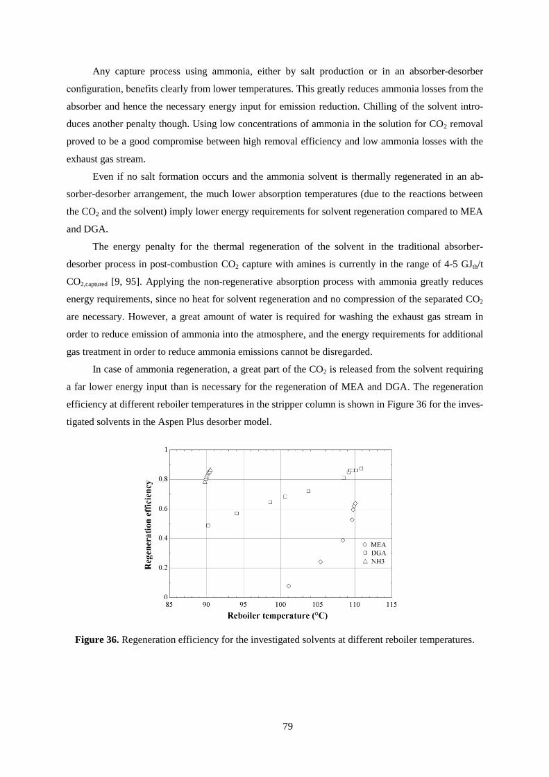
79
Any capture process using ammonia, either by salt production or in an absorber-desorber
configuration, benefits clearly from lower temperatures. This greatly reduces ammonia losses from the
absorber and hence the necessary energy input for emission reduction. Chilling of the solvent intro-
duces another penalty though. Using low concentrations of ammonia in the solution for CO2 removal
proved to be a good compromise between high removal efficiency and low ammonia losses with the
exhaust gas stream.
Even if no salt formation occurs and the ammonia solvent is thermally regenerated in an ab-
sorber-desorber arrangement, the much lower absorption temperatures (due to the reactions between
the CO2 and the solvent) imply lower energy requirements for solvent regeneration compared to MEA
and DGA.
The energy penalty for the thermal regeneration of the solvent in the traditional absorber-
desorber process in post-combustion CO2 capture with amines is currently in the range of 4-5 GJth/t
CO2,captured [9, 95]. Applying the non-regenerative absorption process with ammonia greatly reduces
energy requirements, since no heat for solvent regeneration and no compression of the separated CO2
are necessary. However, a great amount of water is required for washing the exhaust gas stream in
order to reduce emission of ammonia into the atmosphere, and the energy requirements for additional
gas treatment in order to reduce ammonia emissions cannot be disregarded.
In case of ammonia regeneration, a great part of the CO2 is released from the solvent requiring
a far lower energy input than is necessary for the regeneration of MEA and DGA. The regeneration
efficiency at different reboiler temperatures in the stripper column is shown in Figure 36 for the inves-
tigated solvents in the Aspen Plus desorber model.
Figure 36. Regeneration efficiency for the investigated solvents at different reboiler temperatures.

80
So, even if no salt formation occurs and the ammonia solvent is thermally regenerated in an ab-
sorber–desorber arrangement, the much lower absorption temperatures (due to the reactions between
the CO2 and the solvent) imply much lower energy requirements for solvent regeneration as compared
to MEA and DGA.
Using low concentrations of ammonia in the solution for CO2 removal proved to be a good
compromise between high removal efficiency and low ammonia losses with the exhaust gas stream.
Any capture process using ammonia, either by salt production or in an absorber–desorber
configuration, benefits clearly from lower temperatures. This greatly reduces ammonia losses from the
absorber and hence the necessary energy input for emission reduction. However, the energy require-
ments for cooling the solvent and the absorber remain to be investigated. The production of fertilizers
using the ammonia salts produced in the aforementioned process would of course lead to implications
on the fertilizer market and on the producers of these fertilizers. This option will therefore only be
implemented until the level of demand for fertilizers is met and probably in cooperation with the fer-
tilizer producers, which this way could obtain an economical base ingredient from the power plant
sector [90].
81
3.2. Rate-based post-combustion capture models
In order for the simulations of CO2 capture to be more realistic, the kinetics of absorption has to
be taken into account. With reaction kinetics, equipment sizing becomes a factor as well. Here, the
performance of MEA and ammonia at two different solvent temperatures were compared with respect
to their performance as solvent for CO2 capture. Both solvents are thermally regenerated in a stripper
column. Extra care has been taken to reduce solvent emissions to the environment [51, 96].
3.2.1. PC power plant for rate-based post-combustion capture models
The same 500 MW PC power plant as described previously (see 3.1.1) served as basis for the
investigation of the rate-based CO2 capture models.
3.2.2. Rate-based post-combustion CO2 capture with ammonia
Although ammonia has a high loading capacity, the kinetics of CO2 absorption is relatively slow.
Thus, reaction kinetics should be taken into account in the absorption simulations.
Figure 37 shows the flow sheet for the modelled capture process. The cleaned flue gas passes
through a cooler of circulating cold water, where contaminants such as HCl and HF get washed out.
Another advantage is the removal of excess water and the reduction of the volume of the flue gases,
which helps save energy for the flue gas blower (not presented in Figure 37). In order to save energy
for the compression of the captured CO2 and for the reduction of ammonia losses from the desorber,
the stripper column operates at a higher pressure (2 bar). The CO2 rich solvent gets preheated by the
hot lean solvent leaving the desorber. This regenerated solvent needs to be cooled further to the oper-
ating temperature of the absorber column. Before re-entering the absorber, losses of water and ammo-
nia have to be compensated for. Ammonia leaving at the top of both columns is washed out with wa-
ter in additional packed columns. Since also CO2 gets washed out this way, another desorption proc-
ess is necessary to remove it. The remaining water containing the dissolved ammonia has to be sent to
further treatment. In the simulations it was not possible to separate ammonia and water to satisfying
levels in a stripper column. The energy necessary for this water treatment is not included in this study.
Four of the capture installations as shown in Figure 37 are necessary for the removal of CO2 from the
flue gas stream. Their absorber heights and column diameters are 35 m and 11 m, respectively.
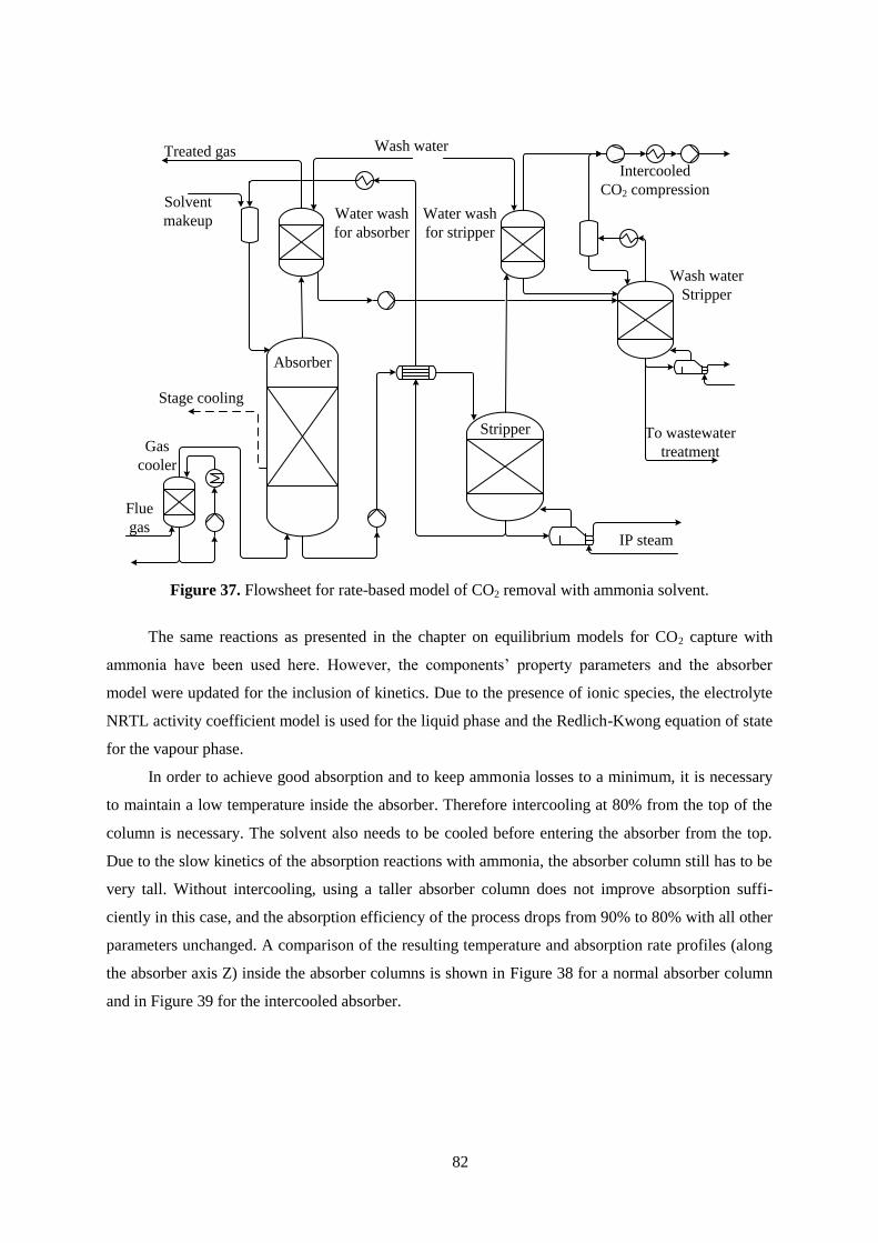
82
Stripper
Water wash
for absorber
Absorber
Gas
cooler
Flue
gas
Solvent
makeup
IP steam
Wash waterTreated gas
Stage cooling
Intercooled
CO2 compression
Water wash
for stripper
Wash water
Stripper
To wastewater
treatment
Figure 37. Flowsheet for rate-based model of CO2 removal with ammonia solvent.
The same reactions as presented in the chapter on equilibrium models for CO2 capture with
ammonia have been used here. However, the components’ property parameters and the absorber
model were updated for the inclusion of kinetics. Due to the presence of ionic species, the electrolyte
NRTL activity coefficient model is used for the liquid phase and the Redlich-Kwong equation of state
for the vapour phase.
In order to achieve good absorption and to keep ammonia losses to a minimum, it is necessary
to maintain a low temperature inside the absorber. Therefore intercooling at 80% from the top of the
column is necessary. The solvent also needs to be cooled before entering the absorber from the top.
Due to the slow kinetics of the absorption reactions with ammonia, the absorber column still has to be
very tall. Without intercooling, using a taller absorber column does not improve absorption suffi-
ciently in this case, and the absorption efficiency of the process drops from 90% to 80% with all other
parameters unchanged. A comparison of the resulting temperature and absorption rate profiles (along
the absorber axis Z) inside the absorber columns is shown in Figure 38 for a normal absorber column
and in Figure 39 for the intercooled absorber.

83
Figure 38. Temperature and absorption rate in absorber column with NH3 solvent (T = 1.7 °C).
It can be seen for the not intercooled absorber that even desorption of CO2 takes place at the
lower end of the column, if there is no intercooling.
Figure 39. Temperature and absorption rate in intercooled absorber with NH3 solvent (T = 1.7 °C).
For the intercooled absorber column, the absorption rate is maintained high along a much larger
part of the column. Therefore, the absorber is used much more efficiently.
For ammonia, solvent performance improves at lower temperatures. Chilled ammonia as an op-
tion for post-combustion CO2 capture was patented [97] in 2006 by Alstom. Alstom proposes a sol-
vent temperature of 1.7 °C [98].
However, at these low temperatures cooling the solvent and intercooling the absorber column
leads to a very significant energy penalty. We therefore investigated an alternative process with a sol-
-0.16
-0.14
-0.12
-0.1
-0.08
-0.06
-0.04
-0.02
0
0.020.0
2.0
4.0
6.0
8.0
10.0
12.0
0 0.2 0.4 0.6 0.8 1
CO
2A
bso
rpti
on
ra
te (
km
ol/
s)
Liq
uid
T (°C
)
Z/Ztotal
Temperature
-0.16
-0.14
-0.12
-0.1
-0.08
-0.06
-0.04
-0.02
0
0.020.0
2.0
4.0
6.0
8.0
10.0
12.0
0 0.2 0.4 0.6 0.8 1
CO
2A
bso
rpti
on
rate
(k
mol/
s)
Liq
uid
T (°C
)
Z/Ztotal
Temperature absorption rate

84
vent temperature of 20 °C. The necessary solvent flow has to be higher, of course, since the loading
capacity of the solvent is lower at this temperature. There is also an increase in the requirements for
solvent makeup, wastewater treatment and above all for heat input to the stripper columns. The over-
all energy penalty of this capture process is discussed in a later section.
For this chilled ammonia process (CAP), the CO2 loading of the lean stream should preferably be
in the range of 0.33 to 0.67 mol of CO2/mol of ammonia, and for the rich stream between 0.67 and 1
mol/mol [99]. In the rate-based simulations here, values at the lower end were found. A lean loading
of 0.32 proved to lead to the lowest energy penalties. This lean loading resulted in rich loadings of 0.5
for the solvent temperature of 1.7 °C and 0.5 for 20 °C, both for a CO2 capture rate of 90%.
A higher desorber pressure reduces ammonia losses and energy requirements for the compression
of the captured CO2, since the pressure is raised by pumping the rich solvent and not by gas compres-
sion. A pressure at the lower end of the recommended range was chosen here due to the size of the
equipment.
In order to find the ideal solvent concentration for the capture process, the author investigated
the necessary solvent flow rate to achieve a given CO2 removal efficiency. With constant lean load-
ing, solvent flow was varied for different solvent concentrations. Figure 40 shows the influence of
ammonia solvent flow and concentration on CO2 removal efficiency in one of the four absorbers nec-
essary for the decarbonisation of the flue gas from the pulverised coal power plant. It can be observed
that due to elevated losses, absorption efficiency is not improved for higher solvent concentrations.
The ideal ammonia concentration was found to be 7.1 %wt.
Figure 40. Removal efficiency for different solvent flows (T = 1.7 °C) and concentrations (% wt.).
50
60
70
80
90
100
800 900 1000 1100 1200
CO
2re
mo
va
l ef
fici
ency
(%
)
Solvent flow (kg/s)
6.07
7.90
11.15
14.85

85
In Figure 41 the influence of reboiler duty on the behaviour of one desorber (of four) is pre-
sented for the base solvent concentration of 7.1 %wt.. Based on the final simulation for 90% CO2 cap-
ture, the reboiler duty was varied for unchanged properties of the incoming CO2 rich stream. In the
base case, a reboiler duty of 103.5 MW was needed to reach a bottom temperature of 100.5 °C in one
of the four stripper columns.
Figure 41. Relative NH3 desorption eff. for varying desorber conditions compared to base case.
97
99
101
103
105
107
60
80
100
120
140
160
180
90 110 130 150 170
reb
oil
er t
emp
era
ture
(°C
)
rela
tive
des
orp
tio
n ef
fici
ency
(%
)
reboiler duty (MWth)
desorption efficiency reboiler temperature

86
The key parameters and results of the capture installations with the ammonia solvent are pre-
sented in Table 33 for the two temperature cases.
Table 33. Key parameters of CO2 capture installation (one of four) with ammonia solvent.
Lean solvent flow and solvent concentration 1336 kg/s, 7.1 %wt. 1596 kg/s, 7.1 %wt.
Gas inlet and solvent temperature 25 °C, 1.7 °C 25 °C, 20 °C
Lean loading 0.318 mol/mol 0.313 mol/mol
Rich loading 0.493 mol/mol 0.450 mol/mol
Column packing Flexipac 1Y,
80% flooding
Flexipac 1Y,
80% flooding
Pressure, height and diameter of absorber column 1.1 bar, 35 m, 10.7 m 1.1 bar, 35 m, 11.2 m
Pressure, height and diameter of stripper column 2 bar, 3 m, 6.8 m 2 bar, 3 m, 7.7 m
Solvent makeup – ammonia, water 1.253 kg/s, 4.450 kg/s 1.880 kg/s, 6.260 kg/s
Wash water flow and temperature 70 kg/s, 15 °C 87 kg/s, 15 °C
Chilling for solvent and absorber intercooling -86.7 MWth -30.1 MWth

87
3.2.3. Rate-based post-combustion CO2 capture with MEA
Due to its higher molecular mass MEA has a lower mass loading capacity than ammonia, and it
has to be regenerated at higher temperatures.
Based on equilibrium models, an ammonia concentration of 28 %wt. was found to lead to the
least energy penalties at a rich loading of 0.67 mol/mol [100]. However, the low molecular mass of
ammonia also facilitates its release with the treated gas from the absorber column, which makes it
necessary to use ammonia in relatively low concentrations of around 8 %wt.
As a compromise between high capture efficiency and solvent losses, which both increase with
solvent concentration, Liu et al. [101] recommend a solvent with 5 to 10 %wt. of ammonia. There-
fore, as presented in Figure 42, the capture efficiency of MEA and ammonia is very similar on a mo-
lar basis. The data presented here were obtained from the CO2 capture models discussed in this thesis.
Starting with a capture efficiency of 90%, the composition (and thus the lean loading) of the lean sol-
vent to the absorber was held constant. Then the solvent flow was reduced down to a CO2 removal
efficiency of 50%.
Figure 42. CO2 removal efficiency for different molar and mass flows of ammonia and MEA.
Plaza et al. carried out experiments with different concentrations of MEA, DEA and ammonia
in aqueous solution in a stirred reaction tank to determine the absorption rates of CO2 at different
temperatures. The ammonia solution (3 %wt. NH3) showed an absorption rate, which was around half
the rate obtained with the MEA solvent (30 %wt. MEA). This means that the absorption columns can
be much smaller for capture operations with MEA. Esber [102] quotes G.T. Rochelle who gives a fac-
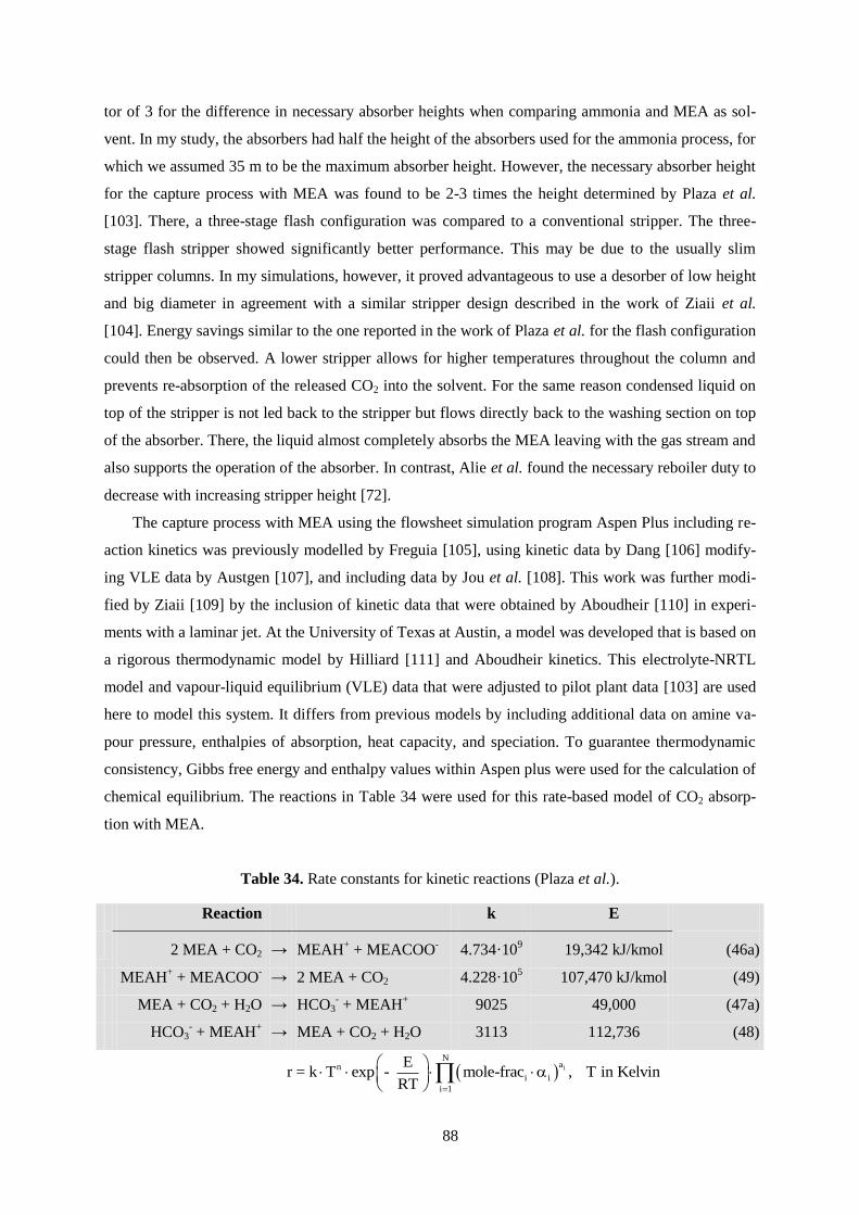
88
tor of 3 for the difference in necessary absorber heights when comparing ammonia and MEA as sol-
vent. In my study, the absorbers had half the height of the absorbers used for the ammonia process, for
which we assumed 35 m to be the maximum absorber height. However, the necessary absorber height
for the capture process with MEA was found to be 2-3 times the height determined by Plaza et al.
[103]. There, a three-stage flash configuration was compared to a conventional stripper. The three-
stage flash stripper showed significantly better performance. This may be due to the usually slim
stripper columns. In my simulations, however, it proved advantageous to use a desorber of low height
and big diameter in agreement with a similar stripper design described in the work of Ziaii et al.
[104]. Energy savings similar to the one reported in the work of Plaza et al. for the flash configuration
could then be observed. A lower stripper allows for higher temperatures throughout the column and
prevents re-absorption of the released CO2 into the solvent. For the same reason condensed liquid on
top of the stripper is not led back to the stripper but flows directly back to the washing section on top
of the absorber. There, the liquid almost completely absorbs the MEA leaving with the gas stream and
also supports the operation of the absorber. In contrast, Alie et al. found the necessary reboiler duty to
decrease with increasing stripper height [72].
The capture process with MEA using the flowsheet simulation program Aspen Plus including re-
action kinetics was previously modelled by Freguia [105], using kinetic data by Dang [106] modify-
ing VLE data by Austgen [107], and including data by Jou et al. [108]. This work was further modi-
fied by Ziaii [109] by the inclusion of kinetic data that were obtained by Aboudheir [110] in experi-
ments with a laminar jet. At the University of Texas at Austin, a model was developed that is based on
a rigorous thermodynamic model by Hilliard [111] and Aboudheir kinetics. This electrolyte-NRTL
model and vapour-liquid equilibrium (VLE) data that were adjusted to pilot plant data [103] are used
here to model this system. It differs from previous models by including additional data on amine va-
pour pressure, enthalpies of absorption, heat capacity, and speciation. To guarantee thermodynamic
consistency, Gibbs free energy and enthalpy values within Aspen plus were used for the calculation of
chemical equilibrium. The reactions in Table 34 were used for this rate-based model of CO2 absorp-
tion with MEA.
Table 34. Rate constants for kinetic reactions (Plaza et al.).
Reaction k E
2 MEA + CO2 → MEAH
+ + MEACOO
- 4.734·10
9 19,342 kJ/kmol (46a)
MEAH+ + MEACOO
- → 2 MEA + CO2 4.228·10
5 107,470 kJ/kmol (49)
MEA + CO2 + H2O → HCO3- + MEAH
+ 9025 49,000 (47a)
HCO3- + MEAH
+ → MEA + CO2 + H2O 3113 112,736 (48)
i
Nan
i i
i 1
Er = k T exp - mole-frac , T in Kelvin
RT
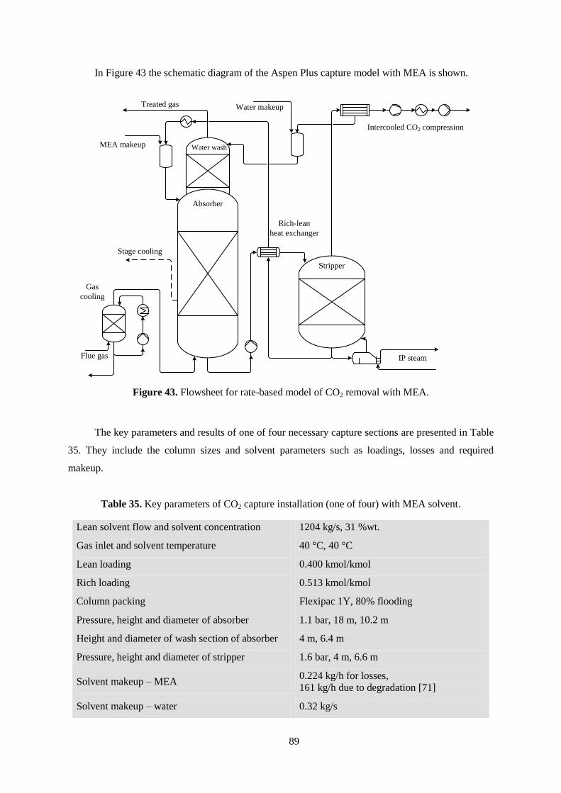
89
In Figure 43 the schematic diagram of the Aspen Plus capture model with MEA is shown.
Stripper
Rich-lean
heat exchanger
Water wash
Absorber
Intercooled CO2 compression
Gas
cooling
Flue gas
MEA makeup
IP steam
Water makeupTreated gas
Stage cooling
Figure 43. Flowsheet for rate-based model of CO2 removal with MEA.
The key parameters and results of one of four necessary capture sections are presented in Table
35. They include the column sizes and solvent parameters such as loadings, losses and required
makeup.
Table 35. Key parameters of CO2 capture installation (one of four) with MEA solvent.
Lean solvent flow and solvent concentration 1204 kg/s, 31 %wt.
Gas inlet and solvent temperature 40 °C, 40 °C
Lean loading 0.400 kmol/kmol
Rich loading 0.513 kmol/kmol
Column packing Flexipac 1Y, 80% flooding
Pressure, height and diameter of absorber 1.1 bar, 18 m, 10.2 m
Height and diameter of wash section of absorber 4 m, 6.4 m
Pressure, height and diameter of stripper 1.6 bar, 4 m, 6.6 m
Solvent makeup – MEA 0.224 kg/h for losses,
161 kg/h due to degradation [71]
Solvent makeup – water 0.32 kg/s

90
In [103], a lean loading of 0.4 mol/mol was shown to present the least energy penalty in CO2 cap-
ture with MEA. Other studies found a lean loading of 0.25 mol/mol [72] or of 0.32 mol/mol [71] to
give the least energy requirements for solvent regeneration. In agreement with literature, a lean load-
ing of 0.3 mol/mol was found this study to give the minimum necessary reboiler duty for solvent re-
generation. However, a hydraulic and a thermal analysis of the absorber revealed that i) more solvent
flow is necessary to prevent liquid being carried out at the top of the absorber and ii) that otherwise
stage temperatures above 76 °C can be found. Therefore, a lean loading of 0.4 was chosen here. For
good absorption, it is necessary to maintain a low temperature inside the absorber. A solvent and gas
inlet temperature of 40 °C was found to give the best results.
In order to achieve this solvent temperature inside the absorber, intercooling at 80% from the top
of the column is necessary here as well. A comparison of the temperature and absorption rate profiles
inside the absorber columns is shown in Figure 44 for a normal absorber column and in Figure 45 for
the intercooled absorber.
Figure 44. Temperature and absorption rate profiles in absorber column with MEA solvent.
-0.16
-0.14
-0.12
-0.1
-0.08
-0.06
-0.04
-0.02
038.0
42.0
46.0
50.0
54.0
58.0
0 0.2 0.4 0.6 0.8 1
CO
2ab
sorp
tion
rate
(k
mol/
s)
liq
uid
tem
per
atu
re (°C
)
Z/Ztotal
Temperature absorption rate

91
Figure 45. Temperature and absorption rate in intercooled absorber column with MEA solvent.
As shown in Figure 40 for ammonia, the ideal solvent concentration was investigated for the
capture process with MEA. Figure 46 shows the influence of MEA solvent flow and concentration on
CO2 removal efficiency in one of the four absorbers necessary for the decarbonisation of the flue gas
from the pulverised coal power plant. It can be observed that in this variation of the base case, com-
pared to the ammonia process, less solvent flow is necessary to achieve a CO2 capture efficiency of
90%.
Figure 46. CO2 removal efficiency for different solvent flows and MEA concentrations (% wt.).
-0.16
-0.14
-0.12
-0.1
-0.08
-0.06
-0.04
-0.02
038.0
42.0
46.0
50.0
54.0
58.0
0 0.2 0.4 0.6 0.8 1
CO
2a
bso
rpti
on
ra
te (
km
ol/
s)
liq
uid
tem
per
atu
re (°C
)
Z/Ztotal
Temperature absorption rate
40
50
60
70
80
90
100
500 600 700 800 900 1000 1100 1200
CO
2re
mo
va
l ef
fici
ency
(%
)
solvent flow (kg/s)
0.25
0.31
0.35
0.48
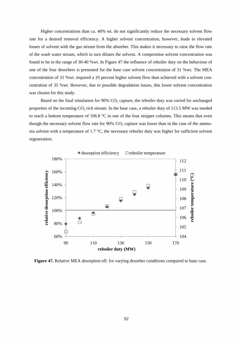
92
Higher concentrations than ca. 40% wt. do not significantly reduce the necessary solvent flow
rate for a desired removal efficiency. A higher solvent concentration, however, leads to elevated
losses of solvent with the gas stream from the absorber. This makes it necessary to raise the flow rate
of the wash water stream, which in turn dilutes the solvent. A compromise solvent concentration was
found to be in the range of 30-40 %wt. In Figure 47 the influence of reboiler duty on the behaviour of
one of the four desorbers is presented for the base case solvent concentration of 31 %wt. The MEA
concentration of 31 %wt. required a 10 percent higher solvent flow than achieved with a solvent con-
centration of 35 %wt. However, due to possible degradation issues, this lower solvent concentration
was chosen for this study.
Based on the final simulation for 90% CO2 capture, the reboiler duty was varied for unchanged
properties of the incoming CO2 rich stream. In the base case, a reboiler duty of 113.5 MW was needed
to reach a bottom temperature of 106.8 °C in one of the four stripper columns. This means that even
though the necessary solvent flow rate for 90% CO2 capture was lower than in the case of the ammo-
nia solvent with a temperature of 1.7 °C, the necessary reboiler duty was higher for sufficient solvent
regeneration.
Figure 47. Relative MEA desorption eff. for varying desorber conditions compared to base case.
104
105
106
107
108
109
110
111
112
60%
80%
100%
120%
140%
160%
180%
90 110 130 150 170
reb
oil
er t
emp
eratu
re (°C
)
rela
tive
des
orp
tion
eff
icie
ncy
reboiler duty (MW)
desorption efficiency reboiler temperature

93
Data for the streams entering and leaving the capture sections with the solvents MEA and am-
monia at the two investigated solvent temperatures (see 3.2.2) are presented in Table 36.
Table 36. Stream data for post-combustion CO2 capture with MEA and ammonia.
MEA Ammonia at 1.7 °C Ammonia at 20 °C
flue gas treated CO2 flue gas treated CO2 waste treated CO2 waste
Temperature
in °C 39.9 40.6 28.5 25 1.8 27.9 100.9 20.4 27.98 104.9
Pressure in bar 1.19 1.1 110 1.19 1.1 110 1.9 1.1 110 1.9
Mass Flow
in kg/sec 590.16 471.72 108.36 567.64 448.00 107.20 230.84 446.05 108.04 285.68
Mole Fractions
H2O 0.0875 0.0699 0.0023 0.027 0.006 0.002 0.968 0.007 0.0022 0.964
CO2 0.1357 0.0153 0.9976 0.145 0.011 0.996 35 ppm 0.008 0.9965 97 ppm
N2 0.7439 0.8761 132.7 ppm 0.793 0.941 0.001 trace 0.944 0.0011 trace
O2 0.0329 0.0387 11.1 ppm 0.035 0.042 114 ppm trace 0.042 100 ppm trace
NH3 -- -- -- -- 595 ppb trace 0.032 1.1 ppm trace 0.036
CO2 capture with MEA leads to a greater purity of the CO2 stream. Higher temperatures in the
capture process lead to a reduced absorption of the lighter gas components and thus to a lower con-
centration of these components in the captured stream.
94
3.2.4. Influence of post-combustion capture (rate-based) on PC power plant performance
In power plants with post-combustion capture it is important to also consider process changes
necessary for the solvents to function properly. For example, NOX and SOX levels have to be reduced
to very low levels [30] upstream of the CO2 capture section, in order to prevent MEA degradation.
This, however, introduces an additional energy penalty to the power plant. With ammonia, these con-
taminants can be captured by the solvent [75]. They would eventually end up in the separated CO2
stream, however, where they may have to be removed to prevent equipment damage due to acid for-
mation. The amount of the ammonia salts (NH4)2SO4 and NH4HCO3 that precipitate under realistic
conditions in the chilled ammonia process remains to be investigated. These salts could be used for
fertilizer production [90].
However, all options studied here assume the same amount of flue gas desulphurisation and deni-
trification prior to CO2 capture and in the power plant without CO2 capture.
The choice of the different capture configurations leads to different impacts on the power plant,
mainly due to the difference in the energy requirements for solvent regeneration in a stripper column,
for which steam is extracted after the medium pressure turbines. The main parameters for power plant
performance without CO2 capture and for a CO2 removal efficiency of 90% are presented in Table 37.
Ciferno et al. [81] investigated the use of aqueous ammonia for CO2 capture and for multi-
pollutant capture based on the Powerspan ECO® process [112], in which the fertilizers (NH4)2SO4 and
NH4NO3 are produced by reaction with the SO2 and the NO2 in the flue gas. The energy penalty found
there for both cases was about half the penalty found in this study and therefore lower than for the
capture option with MEA. However, ammonia losses were not considered in [81] and energy re-
quirements were calculated with the heat of reaction of only three basic equilibrium reactions. No
steam extraction for solvent stripping was assumed to be necessary.
If SOX and/or NOX removal with the ammonia solvent are included, this would lower the energy
penalties for the ammonia process due to a reduction of the energy consumption in the flue gas desul-
phurisation (FGD) section compared to the CO2 capture with MEA. However, the minimum achiev-
able penalty would then still be somewhat higher than the penalty introduced by the MEA process.
Fisher et al. [113] proposed the heat integration of the CO2 compressor with the reboiler of the strip-
per column and obtained energy savings of 5% or 13 MWel. Even more significant savings were pos-
sible by integrating the flue gas cooling with the stripper column. Therefore both heat sources were
used in the simulations to minimize the energy penalty due to CO2 capture [51].
Although ammonia is a more economical solvent, its slow kinetics makes very large absorber
towers necessary, as resulted from the simulations (see 3.2.2). Additional absorbers are necessary to
limit ammonia emission to the atmosphere. Solvent chilling and emission reduction lead to further

95
energy penalties, so that despite the good qualities of ammonia as an absorbent for CO2, the absorp-
tion with MEA is the more economical option here.
Table 37. Parameters for 500 MW PC power plant with and without CO2 capture.
Gross power plant output: 517 MWel
No
Capture
Capture
with MEA
Capture
with NH3
(1.7 °C)
Capture
with NH3
(20 °C)
Blower and pump work for FGD in MWel 21.6+2.2 21.6 + 2.2 21.6 + 2.2 21.6 + 2.2
Reboiler duty (including ammonia wash) in MWth -- 454 414 + 56 540 + 72
Heat integration of gas cooling to reboiler in MWth -- 123 127 125
Heat integration of CO2 compr. to reboiler in MWth -- 47 47 47
Penalty for remaining steam extraction in MWel -- 67 70 104
Flue gas blower and pump work in MWel -- 9 9 9
CO2 compression in MWel -- 31 26 26
Solvent chilling in MWel (COP of chiller = 4.5) -- -- 92 31
Energy savings due to heat integration in MWel -- 41 41 40
Power plant net output in MWel 493 386 296 323
Power plant efficiency (HHV-based) 36.3% 28.4% 21.8% 23.8%
Energy penalty for CO2 capture in MWel -- 107 197 169
Specific energy penalty in GJel/t -- 1.00 1.84 1.58
Specific CO2 production in kg/MWh 868.2 110.9 144.6 132.5
Effective CO2 removal -- 87.2% 83.3% 84.7%
As the simulation results show, the necessary additional gas treatment for the limitation of am-
monia emission introduces a significant energy penalty. For CO2 capture with ammonia at 1.7 °C, this
leads to a combined reboiler duty that is more elevated than in case of capture with MEA. At the
higher solvent temperature, the increase in solvent flow and release of ammonia from the absorber
lead to a further increase in reboiler requirements. This penalty can be reduced by eliminating the
stripper column for the separation of CO2 from the solvent wash. However, the same capture effi-
ciency could only be achieved with higher solvent flows and increased energy for solvent cooling and
reboiler duty in the main stripper. CO2 compression is less energy intensive in case of the ammonia
processes due to the lower temperature of the released CO2.
Solvent chilling presents the biggest energy penalty in case of the model with the lower solvent
temperature for CO2 capture with ammonia. The combined cooling effect of cooling water and chiller
reduces this penalty to about a third for the 20 °C ammonia solvent. Overall energy penalty due to
CO2 capture is significantly larger for use of the ammonia solvent compared to MEA. Therefore, the
effective CO2 removal is also reduced, although all options have a nominal capture efficiency of 90%.

96
Introduction of absorption kinetics lead to higher solvent flows that need to be cooled for the ab-
sorber and heated for stripping. The slower absorption rate with ammonia makes it necessary to use
very tall absorber columns. Together with the extra equipment for the ammonia wash, this leads to
elevated investment costs compared to CO2 capture with MEA [51, 96].
It should, however, be mentioned that a VLE model for the chilled ammonia process described by
Valenti et al. [99] reports a specific energy penalty, which is about 2.4 times lower than the values
given here, although cooling was considered to be achieved with compression chillers.

97
4. Oxy-fuel combustion
A completely different approach to CO2 capture eliminates the need for solvent processes. The
application of oxy-fuel technology as retrofit option for existing power plants was reported to be tech-
nically feasible and at costs comparable to other CO2 capture technologies [114]. In that respect it is
similar to the previously described post-combustion capture. Only minor burner modifications, a new
oxygen injection system and a new flue gas recycle line are needed [12]. The high temperature of the
recycled gas stream leads to an increase in the thermal efficiency of the boiler. However, boiler modi-
fications are more complex due to the need to reduce air leakage to a minimum.
The Oxy-fuel process uses the energy of the fuel by combusting it with pure oxygen, effectively
reducing the nitrogen content and thus the mass flow of the flue gas that has to be treated. Since com-
bustion with pure oxygen leads to combustion temperatures of 3500 °C, the CO2 rich flue gas has to
be recycled to keep the temperature within the limits, which are about 1300-1400 °C for gas turbines
and about 1900 °C for coal-fired boilers [12]. Conditions similar to fuel burning with air lead to a
nearly complete combustion [115] with very low excess oxygen levels of only 1-3% [12]. The flue
gas stream is therefore mainly composed of CO2 and water. Air leakage, not completely pure oxygen
and fuel inerts lead to impurities in the flue gas stream such as NOX, SOX, HCl and Hg as well as the
inerts nitrogen and argon. Due to the lack of nitrogen in the feed gas, the formation of NOX is greatly
reduced [116], leading to reductions of up to 75% when compared to burning with air [117]. The in-
clusion of an SCR section can thus be often avoided as was done in the investigated model.
A key process step in the oxy-fuel technology is the necessary production of nearly pure oxy-
gen, which has a major influence on power plant efficiency. Technologies for O2 production from air
separation are cryogenic distillation, pressure swing adsorption, and polymeric membranes. While for
lower requirements multi-bed pressure swing adsorption may be economical, for larger applications
such as power plants with an oxygen consumption of more than 200 t/d cryogenic air separation is the
economic solution [114]. This technology is also used in pre-combustion capture for the gasification
process. Oxygen production by distillation at cryogenic temperatures [118] has been used for more
than 100 years [12].
Typically, in an air separation plant as shown in Figure 48, air is compressed to 50 to 60 bar
and purified to remove water, CO2, N2O and trace hydrocarbons that could otherwise accumulate to
dangerous levels in oxygen-rich parts of the plant such as the reboiler condenser. This is usually
achieved by switching fixed bed adsorbers with low pressure waste nitrogen as purge stream, where
the absorbers are regenerated either by temperature or by pressure swing. To cool down the air stream
the product nitrogen and oxygen streams are used in a multi-stream aluminium heat exchanger. The
air stream is separated in a double distillation column with aluminium packing. Handling gas streams
with oxygen levels above 40 %vol. must comply with strict rules for metals selection and vapour ve-

98
locity to avoid hazards. The introduced lighter inerts due to unavoidable air leakage need to be re-
moved in the CO2 purification section to produce sufficiently pure CO2 for geological storage or EOR,
so that designing the air separation unit for 95% pure oxygen instead of producing oxygen with 99.5%
purity is more economical [119].
Figure 48. Cryogenic air separation unit [12].
After cooling, compression and drying of the flue gas stream, the impurities are separated from
the CO2 at low temperatures of about -55 °C. The product gas is usually composed of 96% CO2, as
well as nitrogen, argon, oxygen and SO2. For storage, oxygen levels as well as SOX and NOX levels
have to be very low. The required component concentrations in the CO2 product stream are listed in
Table 38. Especially the limit for oxygen levels is crucial, if the CO2 stream is to be used in EOR.
Higher oxygen levels may otherwise cause equipment damage.

99
Table 38. CO2 purity issues for storage and for use in EOR [120].
Components in product CO2 stream For storage For EOR
H2O < 500 ppm < 50 ppm
CO2 > 90% > 90%
SO2 from H&MB < 50 ppm
NO from H&MB from H&MB
O2 < 4 %mol < 100 ppm
Ar + N2 + O2 < 4 %mol < 4 %mol
Regulations for on-shore and off-shore disposal of CO2 are being drafted worldwide. A sensi-
tive issue is the disposal of other wastes such as SOX, NOX and Hg [120].

100
4.1. Oxy-fuel power plant
The third capture option investigated in this study is a 500 MWel Oxy-fuel power plant as pre-
sented in Figure 49 that uses the same coal type as the pulverised coal power plant with post-
combustion CO2 capture. The basic model was developed by Mitsui Babcock, Alstom Power, Air
Products and the IEA GHG R&D programme [119]. This model served as basis for the investigation
of CO2 purification as described in the following subchapters [51].
In order to keep the temperature in the desired range, part of the flue gas is recycled to the
boiler as the secondary recycle flue gas stream. In order to avoid ash accumulation in the boiler and
damage to the recycle fan solids have to be removed in an ESP. The recycle stream must have a tem-
perature of about 300 °C and may need to be premixed with oxygen to promote ignition. The excess
level of oxygen needs to be in the range of 10-20% to ensure sufficient fuel burnout. The theoretical
percentage of oxygen that needs to be added to the recycled gas stream would be in the range of 50
%vol. Due to material constraints, however, oxygen levels in the secondary recycle stream should not
exceed 23 %vol. Therefore, additional oxygen is introduced separately to the boiler.
Coal mill
Fan
Cooler & Dryer
ESP
Coal Heat
exchanger
Primary recycle FG
Impurities
removed
Product FG
Fan
Blower
Secondary recycle FG
O2
Ash
Air Separation Unit
Air
N2
Air ingress
Feed water
HP LPMP
Power
HP
Steam
Condenser
Figure 49. Schematic diagram of 500 MW ASC PC oxy-fuel power plant (after [119]).

101
After a first cooling and drying stage another part of the flue gas is recycled and used for the
preheating and the transport of the coal to the boiler. This primary recycle needs to be cooled, and its
moisture and acid gas components, e.g. SO3 and HCl, need to be removed. Then the recycle is re-
heated before being fed to the coal mills. This stream has to be dry in order to be able to carry the coal
moisture as vapour at low temperatures, since mill exit temperatures are limited to about 60-80 °C due
to risk of ignition and possible coal melting. The temperature of this recycle is limited to 250-300 °C
by the milling equipment. The flow of the secondary recycle stream is also very important to keep
oxygen levels low in the primary recycle due to the risk of explosion in the coal mills [119].
Oxygen of about 95% is supplied by two trains of a three-column ASU with aluminium pack-
ing as presented in Figure 50 with two levels of air compression. Due to unavoidable air ingress, in-
erts always have to be removed in the CO2 purification section. The increase in power to produce
99.5% pure oxygen is greater than the increase in power consumption for CO2 compression there. The
inclusion of a medium pressure column leads to a reduction in power consumption of ca. 10-12%
down to 201 kWh/t, since it minimises the amount of air that needs to be compressed to high pressure
[121].
Compressor 1
3.5 bar
LP
columnair
Compressor 2
5 bar
cold air
HP
column
MP
column
liquid air
N2O2
N2
air
O2
Integration of HP and MPcondensers
with LP reboilers
Dryer
Dryer
Figure 50. Three-column ASU with two levels of air compression (after [121]).
In order to prevent damage to the cryogenic equipment due to blockage or safety problems, wa-
ter vapour, carbon dioxide and other trace hydrocarbons are removed in two dual bed adsorbers.
The main parameters of the IEA GHG 500 MWel oxy-fuel power plant including the ASU are
shown in Table 39. These parameters were obtained by feedback from the authors simulation results
for the flue gas stream to the already existing Excel model at the IEA GHG. Since NOX and SOX will
be removed in the CO2 purification section, there is no need for FGD and De-NOX processes in the

102
power plant. The actual power plant output and efficiency are discussed in a later section, where dif-
ferent CO2 purification systems and their influence on plant performance will be compared.
Table 39. Oxy-fuel power plant parameters [122].
Coal consumption 55.54 kg/s
Heating value coal HHV = 27.06 MJ/kg, LHV = 25.87 MJ/kg
Oxygen excess level 12%
%wt. O2 in the ASU 94.45
%wt. N2 in the ASU 1.72
%wt. Ar in the ASU 3.83
O2 stream supplied from ASU 116.95 kg/s
Amount of air ingress 23.29 kg/s (0.03 kg / kg of flue gas)
Total Flue Gas after the furnace / boiler 772.66 kg/s
Primary recycled FG 150.01 kg/s
Secondary recycled FG 433.98 kg/s
Product Flue Gas 165.94 kg/s
Impurities removed in cooler and dryer H2O 21.64 kg/s, SO3 0.056 kg/s
In order to optimise system performance feed water preheating is achieved by heat integration
with heat rejection from air compressors in the ASU and with the CO2 compressors. This reduces
steam extraction from the low-pressure steam turbine and allows for a higher power output [119].

103
4.2. CO2 flue gas pre-compression and purification
The product flue gas of the Oxyfuel power plant shown in Figure 49 contains about 72 %vol.
CO2 at atmospheric pressure. Before further drying and purification, the flue gas stream needs to be
compressed to about 30 bar. Then all water is removed to prevent blockage in the successive cryo-
genic purification step. There the inerts are removed from the CO2 by liquefying the CO2 at around -
55 °C.
Different patent applications by Air Products, Air Liquide, and by Praxair served the author of
this thesis as basis for the development of Aspen Plus models of the described processes for CO2 pre-
compression and purification [51].
4.2.1. CO2 flue gas pre-compression
Air Products have developed a method of CO2 compression [123] that removes the heavier gas
contaminants such as SO2, NOX, and Hg by reactive distillation in the presence of water and oxygen
prior to the cryogenic CO2 purification. In a first compressor, the flue gas is compressed adiabatically
to 15 bar with no water removal as shown in Figure 51. Intercooling significantly reduces the work
necessary for the compression of the gas stream. However, reduced intercooling to a gas outlet tem-
perature of 307 °C allows for the use of this stream to heat up the inerts leaving the cryogenic purifi-
cation section. These reheated inerts can then expand in a gas turbine in order to recover some of the
compression energy.
After additional cooling down to 30 °C, the gas stream is fed to a distillation column where it is
washed with a recycled condensate stream. In the distillation columns, which were modelled with
RADFRAC blocks, the lead chamber reactions as listed in Table 40 take place. NO is oxidised to
NO2, which then oxidises SO2 to SO3 with NO acting as a catalyst. Then SO3 is converted to sulphuric
acid and NO2 to nitric acid, while the formation of nitric acid only occurs after all SO2 is converted.
The pressure needs to be high for this process because reaction rate increases with pressure to the
third power. Since the gas phase reactions already take place in the heat exchangers due to the high
pressure, they have been modelled with RSTOIC blocks in Aspen Plus. For this section, the VLE
model NRTL was applied, as this EOS resulted in gas compositions closest to the ones reported in the
patent applications.

104
Dist-2
Flue gas
12
Dilute HNO3
14
15
to dryers and cold boxwater
Dist-1
6
dilute H2SO4
HNO3
Hg
9
Intercooled
compressor train
compressor
307 °C
15 bar
3 4
5
7
830 bar
11 13
Figure 51. Reactive pre-compression of CO2 (after [123]).
Before entering the second distillation column, the gas stream is compressed to 30 bar and
cooled down again. Water needs to be added to make up for losses due to the removal of the diluted
acids in the second column.
Table 40. Reactions in reactive compression with distillation [123].
lead chamber reactions phase
NO + 0.5 O2 ↔ NO2 gas, slow (48)
NO2 + SO2 ↔ NO + SO3 gas, fast (49)
SO3 + H2O ↔ H2SO4 liquid, fast (50)
2 NO2 + H2O ↔ HNO2 + HNO3 liquid, fast (51)
2 NO2 ↔ N2O4 liquid, fast (52)
3 HNO2 ↔ HNO3 + 2 NO + H2O liquid, slow (53)
After this process, 95% of the NO are converted and removed as acid, while the conversion rate
for SO2 is about 99.5%. The water content is also effectively reduced by this treatment, leading to a
concentration of about 75 %mol of CO2 in the gas stream.
In Table 41, the key parameters for the flows in this section are compared to an alternative
compression process used for modelling CO2 purification according to patent applications by Air Liq-
uide and Praxair. In the alternative configurations the compression section is held simpler by the
elimination of distillation columns that normally help remove the heavier contaminants from the flue

105
gas stream. Ultra-pure CO2 can then only be obtained by removing these substances with an addi-
tional distillation column in the cryogenic purification section.
As explained in a later section of this thesis, in the case of Air Liquide, the inerts are only
heated up to relatively low temperatures, since the twice expanded inerts stream is used as a coolant.
Therefore, intercooling in the flue gas compressor train can be used to lower the necessary compres-
sion work.
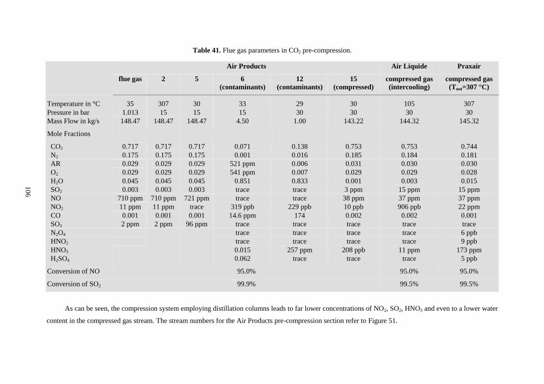
106
Table 41. Flue gas parameters in CO2 pre-compression.
Air Products Air Liquide Praxair
flue gas
2
5
6
(contaminants)
12
(contaminants)
15
(compressed)
compressed gas
(intercooling)
compressed gas
(Tout=307 °C)
Temperature in °C 35 307 30 33 29 30 105 307
Pressure in bar 1.013 15 15 15 30 30 30 30
Mass Flow in kg/s 148.47 148.47 148.47 4.50 1.00 143.22 144.32 145.32
Mole Fractions
CO2 0.717 0.717 0.717 0.071 0.138 0.753 0.753 0.744
N2 0.175 0.175 0.175 0.001 0.016 0.185 0.184 0.181
AR 0.029 0.029 0.029 521 ppm 0.006 0.031 0.030 0.030
O2 0.029 0.029 0.029 541 ppm 0.007 0.029 0.029 0.028
H2O 0.045 0.045 0.045 0.851 0.833 0.001 0.003 0.015
SO2 0.003 0.003 0.003 trace trace 3 ppm 15 ppm 15 ppm
NO 710 ppm 710 ppm 721 ppm trace trace 38 ppm 37 ppm 37 ppm
NO2 11 ppm 11 ppm trace 319 ppb 229 ppb 10 ppb 906 ppb 22 ppm
CO 0.001 0.001 0.001 14.6 ppm 174 0.002 0.002 0.001
SO3 2 ppm 2 ppm 96 ppm trace trace trace trace trace
N2O4 trace trace trace trace 6 ppb
HNO2 trace trace trace trace 9 ppb
HNO3 0.015 257 ppm 208 ppb 11 ppm 173 ppm
H2SO4
0.062 trace trace trace 5 ppb
Conversion of NO 95.0% 95.0% 95.0%
Conversion of SO2 99.9% 99.5% 99.5%
As can be seen, the compression system employing distillation columns leads to far lower concentrations of NO2, SO2, HNO3 and even to a lower water
content in the compressed gas stream. The stream numbers for the Air Products pre-compression section refer to Figure 51.

107
4.2.2. CO2 flue gas purification according to Air Products patent application
As described previously, the CO2 needs to be purified after the pre-compression step. Also for
this process Air Products filed a patent application [124], which the author then modelled in Aspen
Plus. Three alternative configurations described in the aforementioned document were investigated in
detail here.
The compressed flue gas stream passes through a dual bed adsorptive dryer that removes all wa-
ter from the gas stream to prevent ice formation in the cold box. The cold box is a multi-stream heat
exchanger, in which the gas mixture is cooled down to -54 °C by depressurised streams in the system.
In the base case, a first separation of the inert gases is achieved in a flash drum at 30 bar and -33
°C. Thereafter, additional cooling brings the temperature of the gas stream down to -54 °C at which
point the CO2 becomes a liquid and the lighter inert gases can be separated further. The CO2 streams
coming from the flash drums are depressurised to provide cooling to the other streams in the cold box,
while the inerts can be reheated and their expansion work is used in a turbine.
dryers
1
2
8
18
inerts
20
13 14 16 17
10
5
19
6
12
11
9
Purified CO2 stream
1
Cold streams
Hot streams
7
4
Cold box
3
Figure 52. Base case for CO2 purification (after [124]).
As shown in Table 42, this configuration leads to a CO2 purity of 96% with an oxygen content of
0.7 %mol. If greater purity is required, e.g. for the use of the gas stream in EOR, then a stripper col-
umn for separation of the lighter inert gases needs to be included in the purification section. This is
done in the next CO2 purification option shown in Figure 53.

108
dryers
1
2
stripper
4
5
9
8
42
40
41
inerts
44 39
10
20
23 24 26 27
6
43
7
21
22
11
12
38
Purified CO2 stream
1
Cold streams
Hot streams
Figure 53. CO2 purification (Air Products) with stripper column at 17 bar (after [124]).
After a first pass through the cold box, the stream is used to provide heat to the stripper column
in which the liquefied CO2 gets purified. Then the gas is cooled further down to -54 °C, causing the
CO2 to reach liquid state. The major part of the inert gases is then separated in a flash drum, while the
liquid CO2 stream is depressurised to 17 bar and fed to the stripper column. The remaining inerts leav-
ing at the top are recompressed and recycled to the entering gas stream. This facilitates their separa-
tion from the gas mixture in the flash drum. Cooling of the flue gas stream is provided by decompres-
sion of the gas streams of different purity, pressure, and temperature.

109
An alternative version of the previously described Air Products design is presented in Figure
54. It uses two flash stages and a stripper column that is kept at a pressure of 30 bar. Here, two flash
stages are used for separation of the inerts. The first separation occurs at -23 °C and the second at -54
°C. Inerts leaving the stripper column are recycled to increase their concentration in the system and to
improve separation.
dryers
1
2
stripper
4
5
21
20
39
52
53
50
30
23 24 26
27
18
40
19
22
9
Cold box
51
28
29
purified CO2 stream
6 17
78
Cold streams
Hot streams
inerts
Figure 54. CO2 purification (Air Products) with stripper column at 30 bar (after [124]).
A higher pressure in the stripper column should allow for a greater purity of the product CO2
stream. The price to be paid is an increased compression work of the intermediate gas streams. In or-
der to cool the stream entering the stripper column to -8 °C, it needs to expand from a pressure of 78.6
bar. Part of this expansion work is regained by not expanding and recompressing the product stream,
since this stream is extracted from the process as a liquid and then pumped to the required pressure of
110 bar.
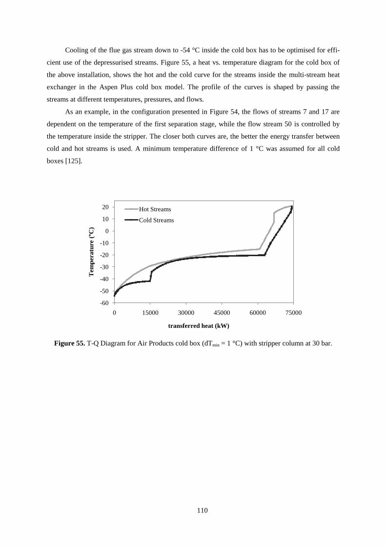
110
Cooling of the flue gas stream down to -54 °C inside the cold box has to be optimised for effi-
cient use of the depressurised streams. Figure 55, a heat vs. temperature diagram for the cold box of
the above installation, shows the hot and the cold curve for the streams inside the multi-stream heat
exchanger in the Aspen Plus cold box model. The profile of the curves is shaped by passing the
streams at different temperatures, pressures, and flows.
As an example, in the configuration presented in Figure 54, the flows of streams 7 and 17 are
dependent on the temperature of the first separation stage, while the flow stream 50 is controlled by
the temperature inside the stripper. The closer both curves are, the better the energy transfer between
cold and hot streams is used. A minimum temperature difference of 1 °C was assumed for all cold
boxes [125].
Figure 55. T-Q Diagram for Air Products cold box (dTmin = 1 °C) with stripper column at 30 bar.
-60
-50
-40
-30
-20
-10
0
10
20
0 15000 30000 45000 60000 75000
Tem
per
atu
re (°C
)
transferred heat (kW)
Hot Streams
Cold Streams
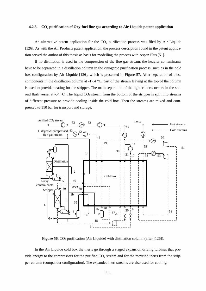
111
4.2.3. CO2 purification of Oxy-fuel flue gas according to Air Liquide patent application
An alternative patent application for the CO2 purification process was filed by Air Liquide
[126]. As with the Air Products patent application, the process description found in the patent applica-
tion served the author of this thesis as basis for modelling the process with Aspen Plus [51].
If no distillation is used in the compression of the flue gas stream, the heavier contaminants
have to be separated in a distillation column in the cryogenic purification process, such as in the cold
box configuration by Air Liquide [126], which is presented in Figure 57. After separation of these
components in the distillation column at -17.4 °C, part of the stream leaving at the top of the column
is used to provide heating for the stripper. The main separation of the lighter inerts occurs in the sec-
ond flash vessel at -54 °C. The liquid CO2 stream from the bottom of the stripper is split into streams
of different pressure to provide cooling inside the cold box. Then the streams are mixed and com-
pressed to 110 bar for transport and storage.
Stripper
3
4
40
18
6
29
5
35
36
Distillation
2
14
421- dryed & compressed
flue gas stream
43
41
3b
4b 48
37
3839
19
20 9
8
23
32
Cold box
11
102130
E-20
33purified CO2 stream
49
52
51
54
53
50
55
heavy
contaminants
inerts
Cold streams
Hot streams
Figure 56. CO2 purification (Air Liquide) with distillation column (after [126]).
In the Air Liquide cold box the inerts go through a staged expansion driving turbines that pro-
vide energy to the compressors for the purified CO2 stream and for the recycled inerts from the strip-
per column (compander configuration). The expanded inert streams are also used for cooling.
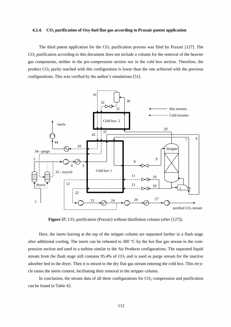
112
4.2.4. CO2 purification of Oxy-fuel flue gas according to Praxair patent application
The third patent application for the CO2 purification process was filed by Praxair [127]. The
CO2 purification according to this document does not include a column for the removal of the heavier
gas components, neither in the pre-compression section nor in the cold box section. Therefore, the
product CO2 purity reached with this configuration is lower than the one achieved with the previous
configurations. This was verified by the author’s simulations [51].
dryers
2
Stripper
67
9
41
4 5
inerts
44
34 - purge
10
20
23 24 26 27
30
42
31
32
21
22
11
12
29
Cold box 2
Cold box 1
8
35 - recycle
33
43
1 E-1
purified CO2 stream
Cold streams
Hot streams
Figure 57. CO2 purification (Praxair) without distillation column (after [127]).
Here, the inerts leaving at the top of the stripper column are separated further in a flash stage
after additional cooling. The inerts can be reheated to 300 °C by the hot flue gas stream in the com-
pression section and used in a turbine similar to the Air Products configurations. The separated liquid
stream from the flash stage still contains 95.4% of CO2 and is used as purge stream for the inactive
adsorber bed in the dryer. Then it is mixed to the dry flue gas stream entering the cold box. This recy-
cle raises the inerts content, facilitating their removal in the stripper column.
In conclusion, the stream data of all three configurations for CO2 compression and purification
can be found in Table 42.

113
Table 42. Stream compositions for the investigated CO2 purification systems.
Air Products
no distillation
Air Products
17 bar
Air Products
30bar Air Liquide Praxair
inerts purified inerts purified inerts purified inerts purified acids inerts purified
Temperature in °C 8.5 28.6 8.5 32.9 8.5 2.3 8.5 32.9 -5.2 8.5 32.9
Pressure in bar 1.1 110 1.1 110 1.1 110 1.1 110 30 1.1 110
Mass Flow in kg/s 36.15 107 39.25 103.90 39.46 103.69 39.32 103.88 0.94 44.96 99.40
Mole Fractions
CO2 0.2780 0.9609 0.2573 0.9997 0.2599 0.9999 0.2573 0.9999 0.9965 0.3314 0.9990
N2 0.5554 0.0242 0.5595 18.5 ppm 0.5572 8.48 ppm 0.5589 20.5 ppm 118 ppm 0.5039 17.2 ppm
AR 0.0840 0.0074 0.0922 14 ppm 0.0920 40 ppm 0.0924 32 ppm 77.2 ppm 0.0828 290 ppm
O2 0.0780 0.0073 0.0863 176 ppm 0.0862 46.5 ppm 0.0867 35.6 ppm 79.3 ppm 0.0776 363 ppm
SO2 6.5 ppb 4.4 ppm 39.2 ppb 4.6 ppm 2.8 ppb 4.6 ppm 61 ppb 11.5 ppm 0.0013 41 ppb 24 ppm
NO 102 ppm 9.56 ppm 114 ppm 0.16 ppm 113 ppm 18.7 ppb 114 ppm 33.2 ppb 61.9 ppb 102 ppm 0.14 ppm
NO2 trace 14.3 ppm trace 14.9 ppb trace 14.9 ppb trace 0.22 ppm 127 ppm 5 ppb 34.70 ppm
CO 0.0046 0.0020 0.0046 0.14 ppm 0.0046 58.5 ppb 0.0046 0.16 ppm 0.91 ppm 0.0041 0.11 ppm
N2O4 trace trace trace trace trace trace trace trace 7.2 ppb trace 9 ppb
HNO2 trace 0 trace 0 trace 0 trace trace 41.2 ppb trace 14.3 ppb
HNO3 trace 0.299 ppm trace 0.311 ppm trace 0.312 ppm trace 54.2 ppb 0.0018 trace 271 ppm
As can be seen from these data, the compression system employing distillation columns leads to far lower concentrations of NO2, SO2, HNO3 and even
to a lower water content. This confirms the findings presented in 4.2.1. The only purification options able to sufficiently reduce oxygen levels to EOR re-
quirements are the Air Products patent application with a stripper column at 30 bar and the Air Liquide configuration (see Table 38).

114
4.3. Influence of CO2 purification on power plant performance
While the previous subchapters were concerned with details of the different configurations for
the CO2 purification process, it is interesting to find out how these configurations affect power plant
performance. As described, leaving the outlet temperature of the first compressor in the reactive com-
pression at 307 °C for heating up the inerts leads to an elevated power consumption in this process.
To see, if the introduction of intercooling would reduce power needs, the author carried out a com-
parative simulation with intercooling of all compressor stages to 30 °C. It was found that the energy
savings (10.75 MWel) due to intercooling are in the same range as the energy regained by the expan-
sion of the inerts, but without the need for an extra turbine [51].
Intercooling, however, increases the complexity of the compressor and requires cooling water.
In any case, if the expansion of the inerts is to be used, the necessary energy for reheating the inerts
should be taken from a part of the power plant where it causes the least penalties. Since the tempera-
ture prior to the expansion of the inerts needs to be about 300 °C, using heat released between com-
pressor stages is adequate. Then the data in Table 43 for capture efficiencies and the important energy
flows that influence power plant performance are obtained for the aforementioned different patent
approaches.
Table 43: Parameters for Oxy-fuel power plant with cryogenic CO2 purification.
Gross power plant output: 584.6 MWel
Gross efficiency (%LHV): 40.7%
no
capture
Air
Products
no
distillation
Air
Products
17 bar
Air
Products
30bar
Air
Liquide
Praxair
Power consumption of ASU in MWel 84.6 84.6 84.6 84.6 84.6 84.6
Nominal capture efficiency -- 87.9% 87.8% 87.6% 87.8% 84.0%
CO2 pre-compression in MWel -- 50.9 50.9 50.9 39.6 48.0
Compression in CO2 purification in MWel -- 10.5 13.1 25.2 10.7 13.4
Expansion in CO2 purification in MWel -- -10.2 -11.1 -11.1 -7.5 -12.5
Power plant net output in MWel 500 449 447 435 457 451
Power plant eff. (%LHV) 34.8% 31.2% 31.1% 30.3% 31.8% 31.4%
Spec. penalty in GJel/t -- 0.492 0.509 0.627 0.412 0.492
Specific CO2 production in kg/MWh 852.1 114.73 116.1 121.5 114.0 151.3
Effective CO2 removal -- 86.5% 86.4% 85.7% 86.6% 82.2%
The CO2 purification according to the Air Liquide patent application shows the highest effec-
tive CO2 removal efficiency due to the lowest energy penalty. In combination with the high CO2 pu-

115
rity achieved here (see Table 42), this option should be given preference over the other purification
configurations. This option also leads to the lowest oxygen levels in the purified CO2 stream. Apart
from the purification according to Air Products with a stripper column at a pressure of 30 bar, it is the
only purification option that produces EOR grade CO2, but at a far lower energy penalty.
The patent application of Praxair needs to be revised because without distillation columns nei-
ther in the pre-compression step nor in CO2 purification, effective CO2 removal and product purity are
low. This is caused by elevated losses of CO2 with the lighter inerts in order to achieve a purity of
99.9%. A higher purity cannot be achieved, as there is no distillation step for the removal of the heav-
ier substances as SOX and NOX.
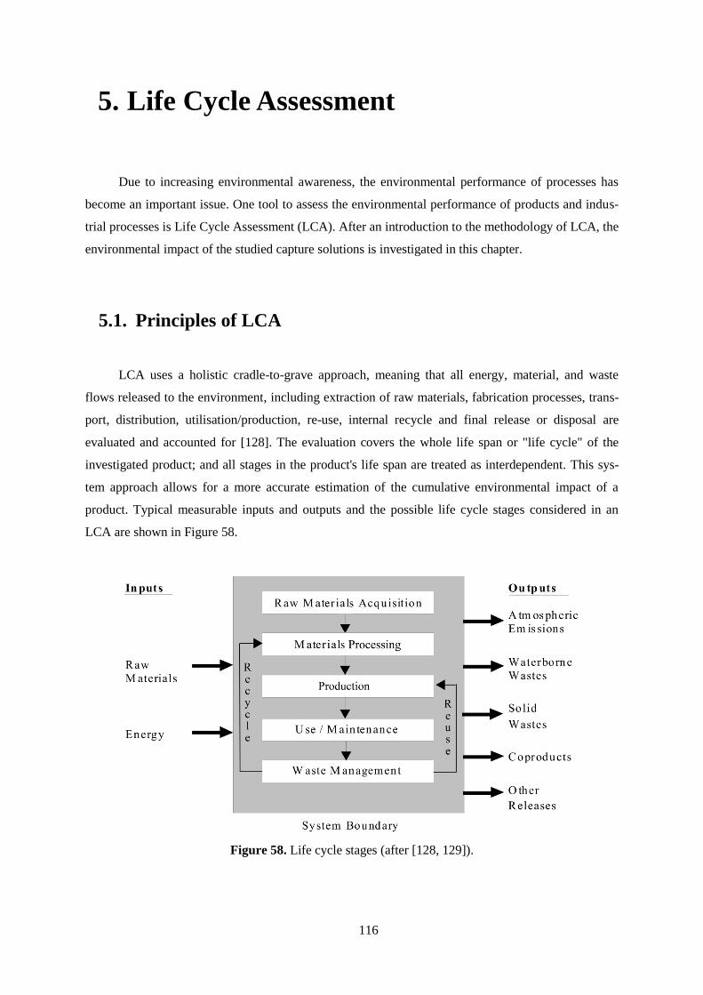
116
5. Life Cycle Assessment
Due to increasing environmental awareness, the environmental performance of processes has
become an important issue. One tool to assess the environmental performance of products and indus-
trial processes is Life Cycle Assessment (LCA). After an introduction to the methodology of LCA, the
environmental impact of the studied capture solutions is investigated in this chapter.
5.1. Principles of LCA
LCA uses a holistic cradle-to-grave approach, meaning that all energy, material, and waste
flows released to the environment, including extraction of raw materials, fabrication processes, trans-
port, distribution, utilisation/production, re-use, internal recycle and final release or disposal are
evaluated and accounted for [128]. The evaluation covers the whole life span or "life cycle" of the
investigated product; and all stages in the product's life span are treated as interdependent. This sys-
tem approach allows for a more accurate estimation of the cumulative environmental impact of a
product. Typical measurable inputs and outputs and the possible life cycle stages considered in an
LCA are shown in Figure 58.
Figure 58. Life cycle stages (after [128, 129]).

117
LCA had its beginnings in the 1960s with the energy analyses of industrial processes by Bous-
tead [89], when large companies started to be concerned about the limitation of raw materials and en-
ergy resources and about environmental issues. In the early 1990s, pressure from environmental or-
ganizations and concerns over inappropriate use of LCA by product manufacturers led to the devel-
opment of international LCA standards [130]. These standards are grouped in the ISO 14000 series.
The development of the international standards (ISO 14040:1997, ISO 14041:1999, ISO 14042:2000,
ISO 14043:2000) was an important step to consolidate procedures and methods of LCA [131]. Their
contribution to the general acceptance of LCA by stakeholders and by the international community
was crucial. These standards were updated in 2006, the new standards now being ISO 14040 and
14044, the latter incorporating the previous standards ISO 14041-14043. In 2002, the international
Life Cycle Initiative was launched by the United Nations Environment Programme (UNEP) and the
Society of Environmental Toxicology (SETAC). The initiative incorporates three programmes that
aim at putting life-cycle thinking into practice and to improve the supporting tools by better data and
indicators [129]. The Life Cycle Management programme produces information materials, establishes
forums for best practice, and carries out training courses all over the world in order to create aware-
ness and to improve the skills of decision makers. The Life Cycle Inventory programme enables
global access to transparent and reliable data by gathering the results of expert groups in web-based
information systems. The Life Cycle Impact Assessment programme is a platform for the exchange of
expert groups in order to establish high quality global life-cycle indicators.
The LCA is a systematic approach, consisting of the following four phases as shown in Figure
59. When deciding between two or more alternatives, LCA can help decision makers compare the
quantity and quality of all major environmental impacts of all phases during the product's life cycle
[128].
- Goal and Scope definition: Definition of the case study and the reasons behind it, definition of
the audience the study is aimed at (Goal).
Definition and description of the investigated product, process or ac-
tivity, its purpose and functional units, as well as the identification of
the boundaries and environmental effects to be considered in the as-
sessment (Scope).
- Inventory Analysis: Identification and quantification of all energy and material flows,
such as raw materials and emissions, as shown in Figure 58.
- Impact Assessment: Assessment of the environmental impacts on human health and eco-
logical effects of all material usage and releases identified in the in-
ventory analysis.

118
- Interpretation: Evaluation of the results of inventory analysis and impact assessment
to enable the selection of the adequate product, process or service
with the identification of uncertainties and assumptions used to gen-
erate the results.
Figure 59. Life Cycle Assessment phases [129].
In the first phase, it is important to define a suitable functional unit as a prerequisite to ade-
quately compare alternative products. The functional unit is the reference unit to which all inlet and
outlet flows will be compared. The definition of the functional unit should be carried out under the
principle of equivalent use. For e.g. alternative beverage containers, the equivalent use basis may be a
fixed quantity of beverage transported to the consumer. The system boundaries are usually defined at
the inlet of raw materials and the emission of waste and/or product flows. It may be necessary to ad-
just these boundaries, if important environmental issues would otherwise be excluded [130].
In the life-cycle inventory, all energy and raw material requirements, atmospheric and water-
borne emissions, solid wastes, and other releases are quantified for the entire life-cycle period consid-
ered in the LCA. The level of detail required depends on the size of the system and the purpose of the
study. In large systems incorporating several industries, some details may not have a major environ-
mental effect. However, great care has to be taken as to the availability and accuracy of the data. The
origin of the data used (measurements, literature, modelling, etc.) should therefore be clearly indi-
cated. Another important point is the allocation of data. The considered mass flows have to be allo-
cated to each production line. Care has to be taken not to duplicate emissions and emissions for the

119
different subprocesses. Recycling, which is often carried out on a global scale may complicate this
allocation process and lead to a readjustment of the system boundaries [130].
In the third LCA phase, the impact assessment, the potential impacts on human health and on
the environment are evaluated, which are caused by the resources and releases identified in the inven-
tory step. For this phase, it has to be decided which impact categories, category indicators and charac-
terisation models will be selected.
The key steps of a Life Cycle Impact Assessment (LCIA) are the following [129, 130]:
- Selection and Definition
of Impact Categories: Identification of relevant environmental impact categories such as
global warming, acidification, ozone depletion.
- Classification: Assigning inventory results to the impact categories (e.g. CO2 emis-
sions to global warming).
- Characterisation: Within the impact categories conversion factors are used to quantify
the impact of the substances from the inventory such as the different
potential impact of CO2 and methane on global warming.
- Normalisation: The potential impacts are referenced to a standard in order to be able
to compare them for different alternatives.
- Grouping: The indicators may be sorted and ranked, e.g. by location (local, re-
gional, global).
- Weighting: Weighting is used to emphasise the importance of potential impacts.
- Evaluation and Reporting: Describing the methodology used, the analysed systems and their
boundaries, and all assumptions made, which helps with understand-
ing the reliability of the LCIA results.
For simplification purposes, LCIA is usually carried out at midpoint level instead of including
all potential effects at specific endpoints, as shown on the example of ozone depletion in Figure 60.

120
Figure 60. Midpoint versus endpoint modelling [132].
Analysis at midpoint level reduces the complexity of modelling and minimizes forecasting and
necessary assumptions, and can therefore provide more comprehensive information that is more
widely accepted.
With the Eco-indicator 95/99 method [133], all substances used or emitted are sorted into
classes according to their effect on the environment as in Figure 61. Substances can be included in
more than one effect class, like NOX, which is toxic, acidifying by forming HNO3, causes eutrophica-
tion, and contributes to ozone depletion. Another example is the emission of SO2, which can cause
damage in the categories acidification and human health. However, the effect depends completely on
the phase in which the SO2 is found. One should thus hypothesize a “phate” scenario (e.g., how much
SO2 is going to the ground, and how much is remaining as a gas) and divide the overall SO2 flow rate
accordingly [133].
A typical example for the characterisation step is the greenhouse effect. The main responsible is
CO2, which has a global warming potential (GWP) of 1. Emissions of CH4 have a GWP of 42, be-
cause methane produces a forty-two times stronger greenhouse effect according to the models used in
SimaPro [131].

121
Figure 61. Principles of the Eco-indicator method [133].
In the normalisation step, another type of scaling is applied in order to gain a better understand-
ing of the relative size of an impact. It is a benchmarking against the known total effect of a class. The
Eco-Indicator method, for example, normalises with effects caused by the average European during a
year.
Not all effects are considered to be equally important. Therefore, the normalised scores are fi-
nally multiplied by a weighting factor, representing the relative importance of the respective effect as
listed in Table 44. The Eco-Indicator 95 and Eco-Indicator 99 weighting is based on a distance-to-
target criterion: the method considers the distance between present value of the category indicator and
the objective value which should be reached at European level. The larger the distance from the tar-
get, the higher is the weight for the category indicator.
In practice, the weighting factor Fi is calculated as [130]:
Fi = Ni/Ti (54)
with
Ni = Current value for effect “i” per person, or “Normalisation Factor”,
Ti = Target value for effect “i”.

122
Table 44. Weighting factors in Eco-indicator 99 method [130].
Effect Weighting factor
Greenhouse effect 2,5
Ozone layer depletion 100
Acidification 10
Eutrophication 5
Summer smog 2,5
Winter smog 5
Pesticides 25
Heavy metals in air 5
Carcinogenic substances 10
As can be seen from this table, in the Eco-Indicator 99 method, the effects are weighted and re-
ferred to three damage macro-categories as shown in Table 45.
Table 45. Damage categories and weighting factors in Eco-indicator 99 method [133].
Damage category Category Indicator Weighting Factor Unit
Ecosystem Quality Potentially Disappeared Fraction (PDF) 400 PDF*m2*yr
Human Health DALY (Disability Adjusted Life Years)
Average Life Expectancy
400 Yr*person
Resource Direct damage to resource 200 MJ/kg
As can be seen from this table, with the Eco-indicator 99 method, the depletion of resources is
given a lower weighting factor than the impact on ecosystem quality and human health.

123
The Eco-Indicator value I results from the weighted sum of all EcoPoints calculated for the dif-
ferent impact categories [130].
ii
ii
EI F
N (55)
with
Ni = Normalisation Value, i.e. current value for Europe of the i-th effect,
Ei = Life Cycle contribution of a product/process to the i-th effect (EcoPoints),
Fi = Weighting Factor = Ni/Ti,
Ti = Target value for the i-th effect.
The interpretation of the LCA results is not just carried out in the final step of the LCA, but for
all steps. The purpose of the interpretation is to check and evaluate the results and to compare them
with the goal and scope definitions. This way, inconsistencies can be identified and necessary adjust-
ments made.
The purpose of an LCA is to inform decision makers by providing a life-cycle perspective of
environmental and human health impacts associated with alternative products or processes. Since
LCA does not take into account technical performance, cost, or political and social acceptance, it is
recommended to use the LCA results in connection with these other social and economic parameters.
All of these parameters should then be based on the same system boundaries and the same functional
unit [129].
This method LCA is not used for absolute evaluation, but rather for comparing the environ-
mental impact of similar products. In the life-cycle approach, the term "product" is also used for proc-
esses and activities.

124
5.2. LCA of rate-based power plant models
The different capture options studied in this thesis reduce the emission of greenhouse gases, but
they also lead to a reduction of the power plant output, i.e. to a higher specific consumption of re-
sources. Especially in post-combustion CO2 capture, the emissions and the necessary production of
the solvents are potentially harmful to the environment.
For a good evaluation of these hazards, a life cycle assessment of the investigated power plants
and capture options is carried out in the following. The commercial software SimaPro 7 with the Eco-
Indicator 99 model was used in this study.
Since the rate-based models include reaction and mass transfer kinetics, only these power plant
and capture models have been considered here. The data, assumptions and results are presented in the
following sub-chapters.
5.2.1. Goal and Scope
This LCA is to give indications to decision makers and the sector of R&D on which capture op-
tions to focus, if the aim is a coal-fired power plant with the lowest environmental impact possible.
The investigated power plants are i) an IGCC with separate and co-capture of CO2 and H2S
with the physical solvent Selexol as pre-combustion capture option, ii) a conventional steam cycle
power plant with post-combustion CO2 capture with the chemical solvents MEA and ammonia, and
lastly iii) an oxy-fuel power plant with CO2 purification to an EOR grade CO2 stream.
As the functional unit for comparison of all power plants the amount of energy produced during
an assumed plant lifetime of 30 years was chosen. All results are therefore referenced to 1 TJel of pro-
duced electricity by the power plants with or without acid gas removal.
The LCA included the impact of raw material extraction, transport, material processing, opera-
tion of the power plant, the use of cooling water and the emissions of flue gases and other substances
during all life-cycle stages. CO2 transport by pipeline and the energy for injection of the captured CO2
into a geological storage site was also included here.
The LCA system boundaries for the PC power plant with and without CO2 capture are shown in
Figure 62 and for the IGCC in Figure 63. The boundaries for the oxy-fuel plant are the same as for the
PC power plant except for the FGD and SCR requirements, since SOX and NOX are removed in the
CO2 purification section.

125
Figure 62. LCA boundaries for PC power plant a) without CO2 capture and b) with capture [134].

126
Figure 63. LCA boundaries for IGCC a) without acid gas removal and b) with removal [134].

127
5.2.2. Life Cycle Inventory
The life-cycle has been divided in three phases: the assembly phase, the operational phase, and
the waste management at the end of the life-cycle.
The assembly phase is the building of the power plant including capture section and CO2 pipe-
line. The amount of materials needed was taken from different sources [134, 135] and include the fuel
necessary for the construction work as well as the transport of the materials over different distances
by road transport as listed in Table 46.
Table 46. Life Cycle Inventory (LCI) of investigated power plant structures.
Material PC power plant Oxy-fuel
power plant IGCC
Capture
Section
MEA
pipeline
Diesel 462 TJ 462 TJ 693 TJ 3 TJ 166 TJ
Electricity 15 GWh 15 GWh 22.5 GWh -- --
Sand -- -- -- -- 97,500 t
Concrete 150,240 t 150,240 t 200,360 t 70 t --
Rock wool 571 t 571 t 856.5 t -- --
Aluminium 332 t 664 t 498 t -- --
Steel (95% low-alloy) 44,801 t 53,761 t 67,202 t 317 t 12,000 t
Copper 710 t 710 t 1065 t 7 t 710 t
Polyethylene 401 t 401 t 601 t 20 t 232 t
Transport (x 103 km) 14,040 t 14,700 t 21,060 t 131 t 380 t
For all metals, material processing such as sheet rolling (steel) and wire drawing (copper) are
included in the LCA. Depending on the size of the capture or purification plant, a factorial approach
was chosen. The multiplication factor was determined by the number and height of absorber towers
relative to the reference capture section with MEA as solvent.
In the operational phase, materials have to be fed constantly to the power plants and capture
sections. Coal has to be extracted and shipped, causing environmental impacts at the mining site and
due to transport by ship, rail and road. Here, the average coal mix used in Europe was used to deter-
mine these impacts. Furthermore, solvent losses have to be compensated for. Additional material is
needed in form of limestone for the FGD section and ammonia for the denitrification of the flue gas.
As an example for the impacts of solvent production, the production process for 1 kg of MEA is
presented in Figure 64. This diagram also includes ammonia production from natural gas by partial
oxidation and steam reforming as well as the use of ethylene oxide. Both substances are necessary for

128
the production of MEA. Furthermore energy and plant infrastructure is needed for the production of
the solvent.
Figure 64. LCA process flow diagram for the production of 1 kg of MEA.
The above diagram also shows the interdepencies of the energy and material flows necessary
for the solvent production. Apart from mass and energy units, this diagram includes Eco-point values,
which will be discussed in the life-cycle impact assessment subchapter.
0.788 kg
A mmonia, liquid, at
regional
storehouse/RER U
0.139 Pt
0.118 kg
A mmonia, partial
oxidation, liquid, at
plant/RER U
0.0295 Pt
0.67 kg
A mmonia, steam
reforming, liquid, at
plant/RER U
0.107 Pt
1.01E-9 p
C hemical plant,
organics/RER/I U
0.0131 Pt
0.734 kg
Ethy lene oxide, at
plant/RER U
0.167 Pt
1 kg
Monoethanolamine,
at plant/RER U
0.351 Pt
4.22 MJ
Electricity , high
v oltage, production
UC TE, at
0.0223 Pt
3.84 MJ
Electricity , medium
v oltage, production
UC TE, at
0.0209 Pt
4.26 MJ
Electricity ,
production mix
UC TE/UC TE U
0.0223 Pt
18.1 MJ
Natural gas, high
pressure, at
consumer/RER U
0.0717 Pt
0.496 m3
Natural gas, at
long-distance
pipeline/RER U
0.0714 Pt
0.207 m3
Natural gas, at
production
onshore/RU U
0.0275 Pt
0.13 m3
Natural gas,
production NL, at
long-distance
0.0166 Pt
0.176 m3
Natural gas,
production RU, at
long-distance
0.0287 Pt
0.261 kg
Heav y fuel oil, at
refinery /RER U
0.0474 Pt
0.258 kg
Heav y fuel oil, at
regional
storage/RER U
0.0477 Pt
0.606 kg
Ethy lene, av erage,
at plant/RER U
0.15 Pt

129
For all plant configurations in the respective chapters of this thesis the incoming material
streams and emissions during operation can be found in the respective chapters of this thesis. These
data were recalculated for a lifetime of 30 years with an average operation of 6,000 h/a at full capac-
ity. Additional solvent to be produced and transported to the power plants was calculated to fill the
used absorber and distillation columns completely. The excess amount compared to operational filling
was assumed to fill the piping in the capture sections. For Selexol, no data could be found in the data-
base of SimaPro. Since losses and makeup were negligible, no major influence of the exclusion of the
process of Selexol production is expected on the results of this LCA. The limestone used for the wet
FGD gets converted to the useful product gypsum. Therefore a beneficial impact of this gypsum pro-
duction is expected. The waste water generated by the washing section to reduce ammonia emissions
are sent to a water treatment plant. Due to uncertainties as to the treatment of the degradation products
of scrubbing with MEA, these data were omitted here. The penalty for dealing with this waste stream
was considered to be negligible in comparison with the penalty for the production and transport of the
necessary solvent makeup. For the waste management at the end of the power plants' life cycle, the
assumptions shown in Table 47 have been made.
Table 47. Waste management for materials used in power plants.
Material Waste scenario
Concrete 100% reuse as filling material for construction work
Rock wool 100% landfill
Aluminium 100% recycling
Steel (95% low-alloy) 80% recycling, 20% landfill
Copper 100% recycling
Polyethylene 100% incineration
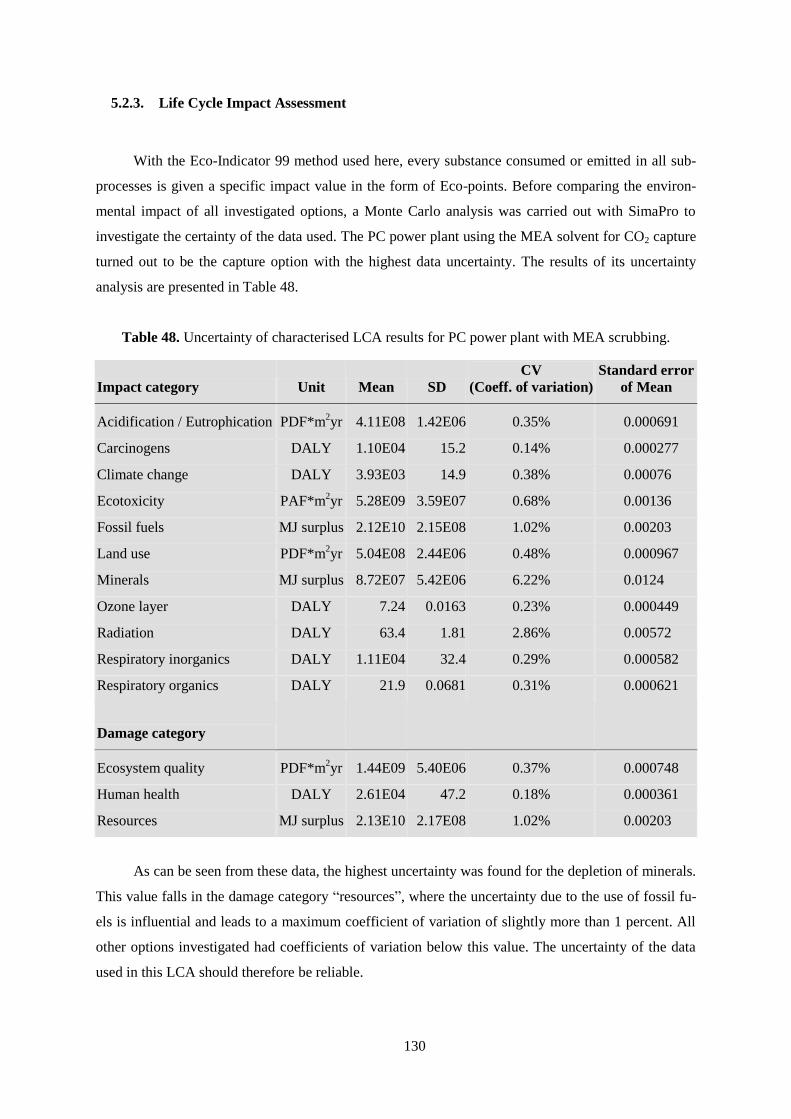
130
5.2.3. Life Cycle Impact Assessment
With the Eco-Indicator 99 method used here, every substance consumed or emitted in all sub-
processes is given a specific impact value in the form of Eco-points. Before comparing the environ-
mental impact of all investigated options, a Monte Carlo analysis was carried out with SimaPro to
investigate the certainty of the data used. The PC power plant using the MEA solvent for CO2 capture
turned out to be the capture option with the highest data uncertainty. The results of its uncertainty
analysis are presented in Table 48.
Table 48. Uncertainty of characterised LCA results for PC power plant with MEA scrubbing.
Impact category Unit Mean SD
CV
(Coeff. of variation)
Standard error
of Mean
Acidification / Eutrophication PDF*m2yr 4.11E08 1.42E06 0.35% 0.000691
Carcinogens DALY 1.10E04 15.2 0.14% 0.000277
Climate change DALY 3.93E03 14.9 0.38% 0.00076
Ecotoxicity PAF*m2yr 5.28E09 3.59E07 0.68% 0.00136
Fossil fuels MJ surplus 2.12E10 2.15E08 1.02% 0.00203
Land use PDF*m2yr 5.04E08 2.44E06 0.48% 0.000967
Minerals MJ surplus 8.72E07 5.42E06 6.22% 0.0124
Ozone layer DALY 7.24 0.0163 0.23% 0.000449
Radiation DALY 63.4 1.81 2.86% 0.00572
Respiratory inorganics DALY 1.11E04 32.4 0.29% 0.000582
Respiratory organics DALY 21.9 0.0681 0.31% 0.000621
Damage category
Ecosystem quality PDF*m
2yr 1.44E09 5.40E06 0.37% 0.000748
Human health DALY 2.61E04 47.2 0.18% 0.000361
Resources MJ surplus 2.13E10 2.17E08 1.02% 0.00203
As can be seen from these data, the highest uncertainty was found for the depletion of minerals.
This value falls in the damage category “resources”, where the uncertainty due to the use of fossil fu-
els is influential and leads to a maximum coefficient of variation of slightly more than 1 percent. All
other options investigated had coefficients of variation below this value. The uncertainty of the data
used in this LCA should therefore be reliable.

131
For comparative reasons the unit Eco-points per TJel of produced electricity during a plant life-
time of 30 years, which here are presented in weighted form according to the seriousness of the envi-
ronmental impact.
The influence of the construction phase and end-of-life phase, including dismantling, reuse, re-
cycling, and disposal, plays only a very minor role for the environmental impact of a power plant with
a lifetime of 30 years is shown in Figure 65 for the case of the PC power plant without capture. For all
configurations with capture the impact of the operation phase is even higher.
Figure 65. Influence of LCA phases on weighted results of PC power plant without CO2 capture.
All environmental impacts of the different power plants with and without CO2 capture are pre-
sented in weighted form with the weighting factors listed in Table 44 and Table 45.
Construction
(0.82%)
Operation
(98.46%)
Waste
management
(0.71%)
Resources 4.98E+06 4.76E+08 2.19E+05
Ecosystem quality 1.22E+06 1.16E+08 6.79E+06
Human health 7.84E+06 1.09E+09 5.16E+06
0.00E+00
3.00E+08
6.00E+08
9.00E+08
1.20E+09
1.50E+09
1.80E+09
Eco
-po
ints

132
All capture options have a nominal capture efficiency of ca. 90% for CO2. The achieved net re-
duction in greenhouse gas emission, however, is significantly lower, as shown in the respective chap-
ters for the effective CO2 capture rate based on the emissions per TJ of produced energy (see 2.3.4,
3.2.4, 4.3). This net capture efficiency reported in the mentioned subchapters is calculated for an en-
dogenous penalty compensation approach (“endo”), i.e. assuming compensation for the drop in the
power plants’ energy output by additional fuel consumption. However, this approach is not very real-
istic, because of the limitations of the investigated power plant. Compensation for energy penalties by
higher fuel consumption is in fact equivalent to compensation by other identical power plants, i.e.
plants with the same net efficiency, in which the same fuel is used and the same capture method ap-
plied. A second more realistic approach to determine the energy compensation of the penalties intro-
duced by CO2 capture considers the amount of compensational energy to be imported from the grid.
In this exogenous compensation approach (“exo”), the environmental impact then depends on the en-
ergy mix used in the considered region [51]. In this study, the energy mix of Italy was assumed to be
the supplier of electricity to the grid. The impact values according to this “exo” approach are higher,
because in Italy electricity is mostly generated by conventional power plants using oil and gas. For
both compensation approaches, the weighted environmental impact due to the emission of greenhouse
gases of all analysed power plant configurations is shown in Figure 66 to Figure 68.
For the IGCC, separate capture of the acid gases led to a slightly higher capture efficiency for
CO2. However, this effect is almost completely compensated for, if exogenous compensation for the
loss in power plant efficiency is taken into account.
For the PC power plant with post-combustion capture, the use of fossil fuels for solvent produc-
tion, especially of oil and gas, in the case of post-combustion capture further reduces the net green-
house effect of CO2 capture to only 49% to 73%, as presented in Figure 67.
For the oxy-fuel power plant, only the plant including CO2 purification is analysed here, since it
would not make much sense to build an oxy-fuel power plant with the penalty introduced by the ASU
without capturing the highly concentrated CO2 in the flue gas stream. The results for the oxy-fuel
plant should therefore be compared with the pulverised coal power plant without CO2 capture. As for
the base case of oxy-fuel flue gas purification, the Air Products patent application without a stripper
column in the cold box section led to a CO2 purity of only about 96%. As the main energy penalty is
caused by the compression of the CO2 and not by the purification process, this base case configuration
had approximately the same detrimental effect on net power output as the other purification configu-
rations, but without resulting in a highly pure CO2 product. This option was therefore excluded from
the LCA.
For pre-combustion capture and the oxy-fuel CO2 purification processes, the contribution of
methane emissions due to coal mining increases, since the net CO2 capture efficiency is higher and
equal to the net capture efficiency reported in the respective chapters with these options. Without CO2
capture, the contribution to the greenhouse effect is directly dependent on power plant efficiency.

133
Figure 66. Impact of GHG emissions for IGCC with and without acid gas removal.
Figure 67. Impact of GHG emissions for PC power plant with and without CO2 capture.
383 309 371 256 1374
0
200
400
600
800
1000
1200
1400
1600
exo endo exo endo
Eco
-Po
ints
per
TJ
elp
rod
uce
d
Remaining substances Carbon dioxide Dinitrogen monoxide Methane
co-capture separate capture no capture
of CO2 and H2S of CO2 and H2S
554 408 764 556 710 519 1510
0
200
400
600
800
1000
1200
1400
1600
exo endo exo endo exo endo
Eco
-Po
ints
per
TJ
elp
rod
uce
d
Remaining substances Carbon monoxide Dinitrogen monoxideMethane Carbon dioxide
MEA NH3 1.7 °C NH3 20 °C no capture

134
Figure 68. Impact of GHG emissions for oxy-fuel power plant with CO2 purification.
As mentioned, the power plants in Italy currently use mainly oil and gas. Therefore the impact
on fossil resource depletion determined by the exogenous compensation approach therefore differs
considerably from the impact caused by higher coal consumption in the power plants with CO2 cap-
ture. This effect is shown in Figure 69 to Figure 71 for the example of resource consumption for all
capture configurations.
385 320 410 331 438 342 407 335
0
50
100
150
200
250
300
350
400
450
500
exo endo exo endo exo endo exo endo
Eco
-Po
ints
per
TJ
elp
rod
uce
dRemaining substances Carbon monoxide Dinitrogen monoxide
Methane Carbon dioxide
Air Liquide Air Products 17 bar Air Products 30 bar Praxair

135
Figure 69. Impacts of resource consumption for IGCC with and without acid gas removal.
Figure 70. Impacts of resource consumption for PC power plant with and without CO2 capture.
1576 1122 1833 1179 1008
0
200
400
600
800
1000
1200
1400
1600
1800
2000
exo endo exo endo
Eco
-Po
ints
per
TJ
elp
rod
uce
dRemaining substances Oil Natural gas Coal
co-capture separate capture no capture
of CO2 and H2S of CO2 and H2S
2544 1626 4011 2782 3910 2904 1190
0
500
1000
1500
2000
2500
3000
3500
4000
4500
exo endo exo endo exo endo
Eco
-Poin
ts p
er T
Jel
pro
du
ced
Remaining substances Oil Natural gas Coal
MEA NH3 1.7 °C NH3 20 °C no capture

136
Figure 71. Impacts of resource consumption for oxy-fuel power plant with CO2 purification.
It can be seen that even without CO2 capture, oil and gas are consumed for coal processing and
transport. Furthermore, in the post-combustion capture options, the production of solvents to make up
for losses and degradation has a very prominent effect on overall fossil fuel consumption [51].
1670 1278 1788 1307 1930 1343 1741 1295
0
500
1000
1500
2000
2500
exo endo exo endo exo endo exo endo
Eco
-Po
ints
per
TJ
elp
rod
uce
d
Remaining substances Oil Natural gas Coal
Air Liquide Air Products 17 bar Air products 30 bar Praxair
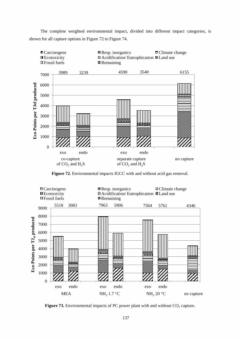
137
The complete weighted environmental impact, divided into different impact categories, is
shown for all capture options in Figure 72 to Figure 74.
Figure 72. Environmental impacts IGCC with and without acid gas removal.
Figure 73. Environmental impacts of PC power plant with and without CO2 capture.
3989 3239 4590 3540 6155
0
1000
2000
3000
4000
5000
6000
7000
exo endo exo endo
Eco
-Po
ints
per
TJ
el p
rod
uce
d
Carcinogens Resp. inorganics Climate change
Ecotoxicity Acidification/ Eutrophication Land use
Fossil fuels Remaining
co-capture separate capture no capture
of CO2 and H2S of CO2 and H2S
5518 3983 7963 5906 7564 5761 4346
0
1000
2000
3000
4000
5000
6000
7000
8000
9000
exo endo exo endo exo endo
Eco
-Po
ints
per
TJ
elp
rod
uce
d
Carcinogens Resp. inorganics Climate changeEcotoxicity Acidification/ Eutrophication Land useFossil fuels Remaining
MEA NH3 1.7 °C NH3 20 °C no capture
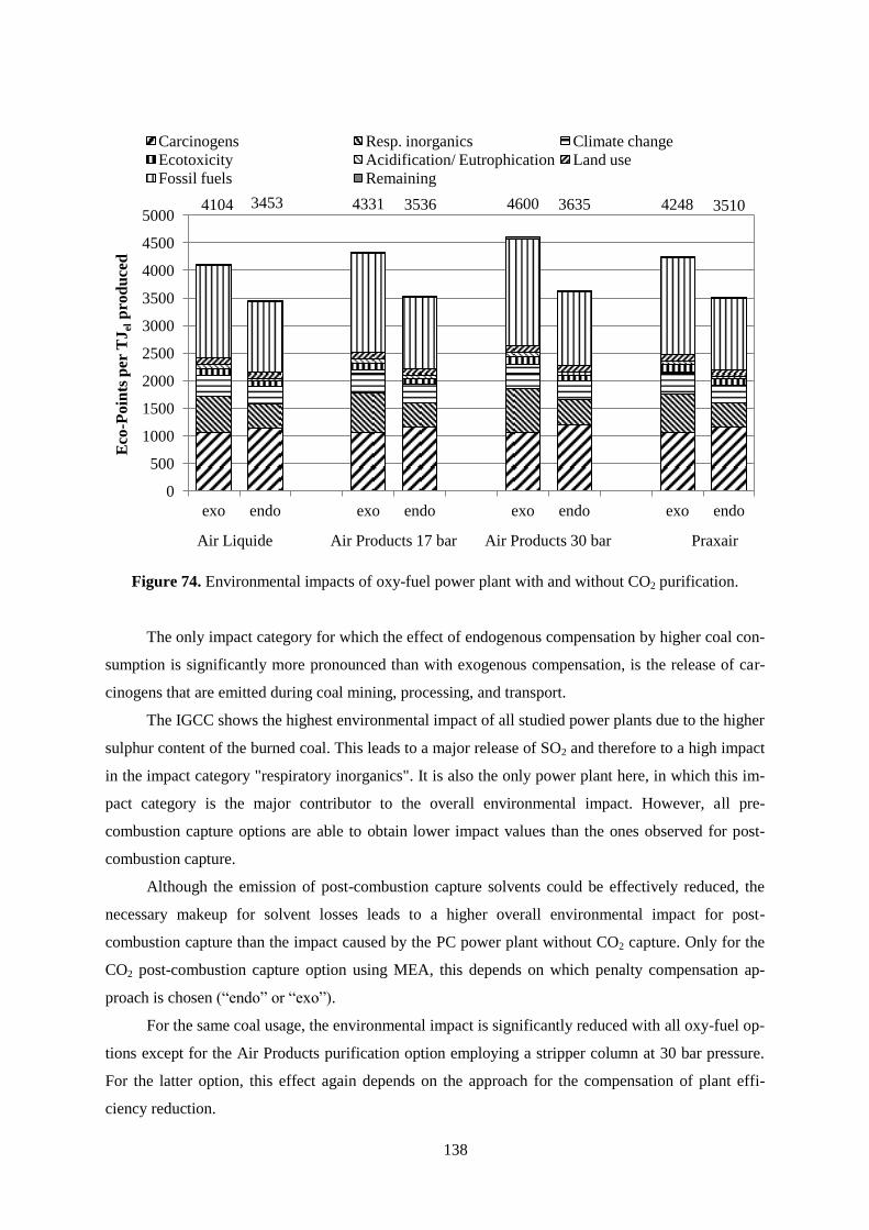
138
Figure 74. Environmental impacts of oxy-fuel power plant with and without CO2 purification.
The only impact category for which the effect of endogenous compensation by higher coal con-
sumption is significantly more pronounced than with exogenous compensation, is the release of car-
cinogens that are emitted during coal mining, processing, and transport.
The IGCC shows the highest environmental impact of all studied power plants due to the higher
sulphur content of the burned coal. This leads to a major release of SO2 and therefore to a high impact
in the impact category "respiratory inorganics". It is also the only power plant here, in which this im-
pact category is the major contributor to the overall environmental impact. However, all pre-
combustion capture options are able to obtain lower impact values than the ones observed for post-
combustion capture.
Although the emission of post-combustion capture solvents could be effectively reduced, the
necessary makeup for solvent losses leads to a higher overall environmental impact for post-
combustion capture than the impact caused by the PC power plant without CO2 capture. Only for the
CO2 post-combustion capture option using MEA, this depends on which penalty compensation ap-
proach is chosen (“endo” or “exo”).
For the same coal usage, the environmental impact is significantly reduced with all oxy-fuel op-
tions except for the Air Products purification option employing a stripper column at 30 bar pressure.
For the latter option, this effect again depends on the approach for the compensation of plant effi-
ciency reduction.
4104 3453 4331 3536 4600 3635 4248 3510
0
500
1000
1500
2000
2500
3000
3500
4000
4500
5000
exo endo exo endo exo endo exo endo
Eco
-Po
ints
per
TJ
elp
rod
uce
d
Carcinogens Resp. inorganics Climate change
Ecotoxicity Acidification/ Eutrophication Land use
Fossil fuels Remaining
Air Liquide Air Products 17 bar Air Products 30 bar Praxair

139
The complete weighted environmental impact, now divided into damage categories according
to the Eco-indicator 99 method, is shown for all capture options in Figure 75 to Figure 77.
Figure 75. Potential environmental damages caused by IGCC with and without acid gas removal.
Figure 76. Potential environmental damages caused by PC plant with and without CO2 capture.
3989 3239 4590 3540 6155
0
1000
2000
3000
4000
5000
6000
7000
exo endo exo endo
Eco
-Po
ints
per
TJ
el p
rod
uce
d
Human Health Ecosystem Quality Resources
co-capture separate capture no capture
of CO2 and H2S of CO2 and H2S
5518 3983 7963 5906 7564 5761 4346
0
1000
2000
3000
4000
5000
6000
7000
8000
9000
exo endo exo endo exo endo
Eco
-Po
ints
per
TJ
elp
rod
uce
d
Human Health Ecosystem Quality Resources
MEA NH3 1.7 °C NH3 20 °C no capture

140
Figure 77. Potential environmental damages caused by oxy-fuel plant with CO2 purification.
The environmental impact grouped into damage categories shows a very high value for poten-
tial damage to human health in case of the IGCC without acid gas removal. This value is greatly af-
fected by the release of SO2. However, all pre-combustion capture options lead to similar environ-
mental impacts, as observed for the oxy-fuel power plant with CO2 purification.
The highest impact values for the power plants with capture, especially in the damage category
"resources", are obtained for the post-combustion capture options. Here, the necessary solvent
makeup due to losses and degradation leads to a major consumption of fossil fuels for solvent produc-
tion [51].
4104 3453 4331 3536 4600 3635 4248 3510
0
500
1000
1500
2000
2500
3000
3500
4000
4500
5000
exo endo exo endo exo endo exo endo
Eco
-Po
ints
per
TJ
elp
rod
uce
d
Human Health Ecosystem Quality Resources
Air Liquide Air Products 17 bar Air Products 30 bar Praxair

141
5.2.4. Interpretation of LCA results
The IGCC shows the highest energy efficiency of all options studied here, and the penalties in-
troduced by CO2 capture are the lowest as well. Therefore, the environmental impact due to fossil fuel
consumption is the lowest for this power plant. Due to the low energy penalty introduced by the use of
physical solvents, pre-combustion acid gas removal has also one of the lowest overall environmental
effects here. Furthermore no additional harmful substances, e.g. solvents, are emitted, which also
leads to a negligible impact caused by solvent production. The total impact of the IGCC may be fur-
ther reduced by the use of coal with a lower sulphur content.
Of the post-combustion capture options only the use of MEA is capable of reducing the overall
environmental impact according to the Eco-indicator 99 method. However, solvent production leads
to a major environmental impact due to fossil resource consumption. Solvent emissions are consid-
ered harmful respiratory inorganic substances, i.e. they are potentially dangerous to the human health.
However, if MEA is to be used, solvent degradation needs to be minimised thorough desulphurisation
and denitrification, and possibly also by addition of corrosion inhibitors. For ammonia, alternative
processes are necessary to minimise or recuperate ammonia losses due to the high volatility of the
solvent.
In the oxy-fuel power plant, compression and purification of the CO2 do not introduce a large
penalty. However, due to the large energy requirements for the ASU and for the gas recycle blowers,
this power plant has a relatively low energy efficiency. However, with the expected development of
more efficient air separation, the energy efficiency is expected to increase [119], leading to a reduced
environmental impact.
It can be seen for the majority of impact categories that the impact of energy penalties intro-
duced by CO2 capture is more harmful, if the penalties are compensated for by electricity production
in other power plants (according to the energy mix of the considered region Italy) rather than by addi-
tional fuel consumption in the investigated power plants. The latter is equivalent to the compensation
of the decrease in energy output by identical power plants, i.e. by coal power plants with CO2 capture
[51]. The unfavourable effect of exogenous compensation shown here can be explained by the fact
that in Italy most energy is still produced by conventional fossil fuel power plants without CO2 cap-
ture. The impact of this exogenous compensation may eventually become lower, when a transition to
low-carbon power production is made. In other regions with a different energy mix than Italy, the en-
vironmental impacts will also be different then.
142
6. Exergetic Life Cycle Assessment
As shown in the previous chapter, the environmental sustainability of processes can be evalu-
ated and compared within the framework of the well-established methodology of Life Cycle Assess-
ment [136, 137]. However, until recently the concept of exergy as a measure for sustainability was
omitted from this analysis. Exergy and the depletion of natural resources are directly related, as de-
scribed by Cornelissen [138]. Therefore, the traditional LCA can be improved by applying this exergy
concept, resulting in Exergetic Life Cycle Assessment (ELCA).
6.1. Principles of ELCA
Exergy can be regarded as a measure for available energy. Exergy analysis is used to determine
the amount of potential work lost during a process and to identify the sources of the greatest losses.
For the calculation of the exergy content of a stream, the main components are physical and chemical
exergy. Kinetic, potential, nuclear and magnetic influences are usually neglected. The total exergy
content of a stream is then calculated by
e = eph + ech (56)
Physical exergy eph is defined to be equal to the maximum amount of work obtainable when the
stream of a substance is brought from its initial state to the environmental state by physical processes
involving only thermal interaction with the environment [139]. The environmental is defined by the
pressure p0 and the temperature T0 .
The physical exergy of a stream is then given by
eph = h – h0 – T0 · (s – s0) (57)
Here h and s are the enthalpy and the entropy of the stream at its temperature T and its pressure
p. The properties h0 and s0 are the same properties at the environmental conditions T0 and p0.
Chemical exergy ech is defined to be equal to the maximum amount of work obtainable by
bringing a substance from the environmental state to the dead state by processes involving heat trans-
fer and exchange of substances only with the environment [139].
So, while for the calculation of physical exergy, the final state of the stream is the environ-
mental state, for the calculation of chemical exergy the latter is the initial state. The final state in the

143
case of chemical exergy, the dead state, is reached, when the substance is in thermal, mechanical, and
chemical equilibrium with the environment. The tabulated reference values for the substances are ob-
tained at the environmental and partial pressure at which they exist in the environment.
For a mixture of ideal gases the chemical exergy is calculated by
ch i i 0 i i
i i
e x · e R T · x · ln x (58)
The last part of the equation is identical to the Gibbs energy of mixing
mix i i
i
dG n R T· x · ln x (59)
This means that the chemical exergy is the sum of the exergy of the components and the contri-
bution of mixing the pure components [139].
In all real world processes exergy is consumed as entropy is produced [140, 141]. The so-called
exergy destruction is proportional the total entropy production
dE = T0 · dS
(60)
Here T0 is the temperature of the environment.
The exergy balance can also be written as
Ėin + Ėq = Ėout + İ + Ẇ
(61)
Ėin and Ėout represent the exergy associated with the mass streams, while Ėq represents the ex-
ergy of heat and Ẇ the work exchanged with the environment. From the second law of thermody-
namic follows that the irreversibility İ has to be positive.
An exergy analysis can be used to determine the thermodynamic perfection of a system and to
show where the work potential of natural resources in relation to the surrounding environment is lost
[142]. The maximum work is obtained in a completely reversible process.

144
In an ELCA, all irreversibilities of the investigated processes are considered for their entire life-
time, so that all life cycle stages have to be included. Furthermore, it is important to not include only
the processes within the system, but also the processes related to all incoming and outgoing material
and energy streams. A first step was the introduction of the Cumulative Exergy Consumption (CExC)
of a product, i.e. the total exergy consumption from the extraction of raw materials to the final product
[143]. However, this method does not take into account the exergy destruction associated with the
disposal, recycling, or reuse of the product [138].
The irreversibilities due to emissions and the depletion of resources of a non-ideal process can
be identified with an exergy analysis. On the basis of such an analysis, it is possible to compare the
environmental burden of the investigated processes caused by exergetic resource consumption and
emissions. A special case are the zero-exergy emission processes. There all emissions are harmless to
the environment because their chemical composition and physical properties are identical to the envi-
ronment itself [138]. In this case the ELCA will give the same ranking as a conventional LCA, while
being able to provide information on the location of the major process irreversibilities. In the special
case of a so-called Zero-ELCA, the exergy consumption for the reduction of all harmful emissions to
zero in an additional process is included. With the inclusion of this abatement exergy, the life cycle
irreversibility can be used as single criterion for the comparison of different processes with the same
function, since all other environmental effects will be similar.
Both the LCA and the ELCA have a similar framework with identical goal and scope defini-
tions. If the aim of the ELCA is to identify the process components with the highest irreversibilities or
exergy destruction, the inventory has to be much more extensive than in the case of an LCA. A com-
plete flowsheet of the mass and energy streams in the different process steps is then required, and all
energy and mass balances need to be closed. A more simplified black box approach may be used if the
aim is to compare complete systems. Then, as in an LCA, only the inputs and outputs of the investi-
gated processes are considered.

145
6.2. Exergy analysis of rate-based power plant models
In order to determine the performance of the investigated capture options in terms of process ir-
reversibilities and exergetic efficiencies, an exergy analysis was carried out for the same key proc-
esses as in the LCA in the previous chapter.
As a first step all important inputs and outputs of the power plants were identified. For the
IGCC with and without pre-combustion capture these exergetic inputs and outputs are shown in
Figure 78.
Slurry water
Work streams
Material streams
Net power output
Compressed CO2
Coal
Grey water for de-NOX
Excess liquid from WGS
Air for separation in ASU
HP nitrogen stream
IGCC
Stack gas
Acid gas stream
Figure 78. Main exergy stream for IGCC with and without acid gas removal.
The flows and exergy contents of the important inputs and outputs of the IGCC are summarised
in Table 49.
For the pulverised coal power plant these streams are shown in the form of a diagram in Figure
79, and the data for these streams can be found in Table 50.
For all processes, only the streams directly connected to the power plants were considered here.

146
Table 49. Exergies of main energy and mass flows of IGCC.
Stream
mass flow
(kg/s)
exergy
(kJ/kg)
Ėch
(kW)
Ėph
(kW)
Exergy
(kW)
Coal 43.8 29441.0 1288000.0 0.0 1288000.0
Slurry water 23.5 3637.0 16214.0 69360.0 85574.0
Air for separation in ASU 170.1 0.7 113.5 0.0 113.5
HP nitrogen from ASU 125.2 757.8 20169.0 74686.0 94856.0
Grey water for de-NOX 18.3 65.5 1196.0 0.0 1196.0
Excess liquid from WGS 29.0 310.9 7269.0 1755.0 9024.0
Stack gas (no capture, no shift) 694.4 77.6 34556.0 19345.0 53901.0
Stack gas (separate capture) 656.3 66.3 10165.0 33361.0 43526.0
Stack gas (co-capture) 652.8 56.1 10697.0 25904.0 36601.0
Acid gas stream (separate capture) 3.1 1350.0 3976.0 261.6 4238.0
Compressed CO2 (separate capture) 73.4 706.8 33135.0 18737.0 51872.0
Compressed CO2 (co-capture) 73.8 706.8 33311.0 18837.0 52147.0
Net power output (no capture, no shift)
456300.0
Net power output (separate capture)
392500.0
Net power output (co-capture)
412500.0
Combustion air
Work streams
Material streams
Net power output
Compressed CO2
Coal
Limestone slurry
Gypsum
Ammonia for SCR
Solvent makeup
PC
power
plant
Stack gas
Wash water
Figure 79. Main exergy stream for PC power plant with and without CO2 capture.
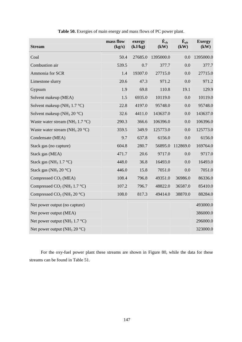
147
Table 50. Exergies of main energy and mass flows of PC power plant.
Stream
mass flow
(kg/s)
exergy
(kJ/kg)
Ėch
(kW)
Ėph
(kW)
Exergy
(kW)
Coal 50.4 27685.0 1395000.0 0.0 1395000.0
Combustion air 539.5 0.7 377.7 0.0 377.7
Ammonia for SCR 1.4 19307.0 27715.0 0.0 27715.0
Limestone slurry 20.6 47.3 971.2 0.0 971.2
Gypsum 1.9 69.8 110.8 19.1 129.9
Solvent makeup (MEA) 1.5 6935.0 10119.0 0.0 10119.0
Solvent makeup (NH3 1.7 °C) 22.8 4197.0 95748.0 0.0 95748.0
Solvent makeup (NH3 20 °C) 32.6 4411.0 143637.0 0.0 143637.0
Waste water stream (NH3 1.7 °C) 290.3 366.6 106396.0 0.0 106396.0
Waste water stream (NH3 20 °C) 359.5 349.9 125773.0 0.0 125773.0
Condensate (MEA) 9.7 637.8 6156.0 0.0 6156.0
Stack gas (no capture) 604.8 280.7 56895.0 112869.0 169764.0
Stack gas (MEA) 471.7 20.6 9717.0 0.0 9717.0
Stack gas (NH3 1.7 °C) 448.0 36.8 16493.0 0.0 16493.0
Stack gas (NH3 20 °C) 446.0 15.8 7051.0 0.0 7051.0
Compressed CO2 (MEA) 108.4 796.8 49351.0 36986.0 86336.0
Compressed CO2 (NH3 1.7 °C) 107.2 796.7 48822.0 36587.0 85410.0
Compressed CO2 (NH3 20 °C) 108.0 817.3 49414.0 38870.0 88284.0
Net power output (no capture)
493000.0
Net power output (MEA)
386000.0
Net power output (NH3 1.7 °C)
296000.0
Net power output (NH3 20 °C)
323000.0
For the oxy-fuel power plant these streams are shown in Figure 80, while the data for these
streams can be found in Table 51.

148
Work streamsMaterial streams
Net power output
Compressed CO2
Coal
Water and SO3 removed in cooler and dryer
Air for separation in ASU HP nitrogen stream
Oxy-fuel
power
plant
Inerts
Sour compression condensate
Figure 80. Main exergy stream for oxy-fuel power plant with CO2 purification.
Table 51. Exergies of main energy and mass flows of oxy-fuel power plant.
Stream
mass flow
(kg/s)
exergy
(kJ/kg)
Ėch
(kW)
Ėph
(kW)
Exergy
(kW)
Coal 55.5 27685.0 1538000.0 0.0 1538000.0
Air for separation in ASU 506.3 0.7 337.8 0.0 337.8
HP nitrogen from ASU 384.2 649.2 20169.0 229208.0 249377.0
Water and SO3 removed in cooler and dryer 22.0 2991.0 1170.0 64624.0 65794.0
Condensate Air Products 5.5 357.2 1964.0 0.0 1964.0
Condensate Air Liquide 5.7 379.1 2179.0 0.0 2179.0
Condensate Praxair 4.8 365.0 1765.0 0.0 1765.0
Inerts (Air Products 17 bar) 39.3 131.8 5169.0 6.2 5175.0
Inerts (Air Products 30 bar) 39.5 132.9 5237.0 6.2 5244.0
Inerts (Air Liquide) 39.3 131.7 5172.0 6.2 5179.0
Inerts (Praxair) 39.3 131.8 5169.0 6.2 5175.0
Compressed CO2 (Air Products 17 bar) 103.9 706.8 46901.0 26521.0 73422.0
Compressed CO2 (Air Products 30 bar) 103.7 706.8 46815.0 26473.0 73288.0
Compressed CO2 (Air Liquide) 103.9 706.8 46923.0 26534.0 73457.0
Compressed CO2 (Praxair) 104.0 706.8 46955.0 26552.0 73507.0
Net power output (no capture)
500000.0
Net power output (Air Products 17 bar)
447000.0
Net power output (Air Products 30 bar)
435000.0
Net power output (Air Liquide)
457000.0
Net power output (Praxair)
451000.0

149
In Table 52, the calculated irreversibilities and exergetic efficiencies of the power plants are
listed. Here, the irreversibility or exergy destruction is calculated according to
ĖD = Ėin – Ėout (62)
And the simple exergetic efficiency is defined by
out
in
E
E (63)
For most processes, the output is not only the product but in part also waste.
Ėout = Ėproduct + Ėwaste (64)
For the exergetic efficiencies based on the useful product of the process, the following defini-
tion for the so-called rational exergetic efficiency [139] is used:
product
in
E
E (65)
The exergy efficiency obtained by this definition depends strongly on which process outputs
are considered as useful products.
Both definitions have been applied in the exergy analysis of the power plants. In Table 52, their
exergy destruction and exergetic efficiencies are reported. Three different options were considered for
the definition of the product of the power plants. The first option considers the produced power to be
the only useful product here. The second option also considers the use of the compressed CO2 stream,
e.g. in EOR operations, while the last efficiency value includes the use of the compressed nitrogen
stream leaving the ASU. In the case of CO2 purification in oxy-fuel combustion, this nitrogen stream
could be used for power generation in a turbine when being mixed to the separated inerts.

150
Table 52. Exergy destruction ĖD and exergetic efficiencies of all power plant configurations.
Capture option
ĖD
(MW)
ε
ψ
(electricity)
ψ
(+ CO2)
ψ
(+ N2)
Pre-combustion capture
No capture 761 44.7% 33.2% -- 40.1%
Separate capture 779 43.4% 28.5% 32.6% 39.5%
Co-capture 770 44.0% 30.0% 33.8% 40.7%
Post-combustion capture
No capture 764 46.5% 34.6% -- --
MEA 949 34.0% 26.9% 32.9% --
NH3 (1.7 °C) 1018 33.2% 19.4% 25.0% --
NH3 (20 °C) 1026 34.7% 20.6% 26.2% --
Oxy-fuel
Air Products (17 bar) 827 48.4% 27.9% 32.4% 48.0%
Air Products (30 bar) 839 47.7% 27.1% 31.7% 47.2%
Air Liquide 817 49.1% 28.5% 33.1% 48.6%
Praxair 823 48.7% 28.1% 32.7% 48.2%
The difference between the simple exergetic efficiency ε and the exergy definition distinguish-
ing between exergy product and losses shows that a significant amount of the exergy leaving the
process is lost. For more efficient energy generation these losses should be reintegrated to the power
plants whenever and wherever possible. If for example the exergy content of the compressed nitrogen
stream from the ASU could be used either in the gasification process or by expansion in a turbine,
exergy losses could be reduced to a minimum. In the case of post-combustion capture, losses are
caused by solvent degradation (MEA) and to a significant amount by solvent losses in the case of
ammonia. These losses cannot be compensated for.
With electricity as the only useful product, the highest rational exergy efficiency ψ was ob-
served for pre-combustion acid gas removal. If the compressed nitrogen stream were to be integrated,
the highest exergy efficiency would be obtained with the oxy-fuel processes.

151
6.3. ELCA of rate-based power plant models
For the investigated power plant configurations, the same lifetime as in the LCA was assumed,
i.e. the power plants run an average of 6000 h/a at 100% capacity for 30 years. The goal and scope
definition as well as the complete inventory for the different power plants with and without CO2 cap-
ture can be found in chapter 5.2, where the Life Cycle Analysis of these power plant configurations
was discussed. The possible use of the compressed CO2 in EOR and the use of the compressed nitro-
gen were disregarded in this ELCA. However, as listed in Table 53, the Cumulative Exergy Con-
sumption (CExC) of the used materials for the power plant construction was taken into account [144].
Table 53. Cumulative exergy consumption of resources and utilities for plant construction.
Material or Utility CExC
Concrete 1.1 MJ/kg
Rock wool 21.1 MJ/kg
Aluminium 250 MJ/kg
Steel (95% low-alloy) 54 MJ/kg
Copper 67 MJ/kg
Polyethylene 86 MJ/kg
Truck transport 3.13 MJ/tkm
Table 54. CExC and end-of-life irreversibilities related to power plant construction.
Capture option CExC CExC + waste scenario
Pre-combustion capture
No capture 5883.2 11001
Separate capture 5905.9 11044
Co-capture 5928.7 11086
Post-combustion capture
No capture 4249.9 7947
MEA 4272.7 7990
NH3 4295.5 8033
Oxy-fuel
All configurations 4771.1 8922

152
Since the CExC values do not include the exergy destruction at the end of the life cycle of the
power plants [138], the same relationship as found in Figure 65 was used to include this influence
here. The total CExC and the end-of-life exergy destruction of the used materials are shown in Table
54.
For the power plants already selected in the previous chapter on Life Cycle Assessment of the
rate-based capture options, the cumulated irreversibilities or exergy destruction over the entire life
cycle are presented in Figure 81 to Figure 83. The environmental cost for coal mining, processing, and
transport was included here and found to be an additional 3 per cent of the exergy content of the used
coal [145].
Figure 81. Life cycle irreversibilities of IGCC with and without acid gas removal.
The addition of acid gas removal to the power plant leads only to a minor increase in exergy
destruction inside the power plant. Here, the co-capture of H2S and CO2 had a lower exergetic impact
than the separate capture of these acid gas components.
5.25E+05 5.37E+05 5.31E+05
0.00E+00
1.00E+05
2.00E+05
3.00E+05
4.00E+05
5.00E+05
6.00E+05
no capture separate capture co-capture
Exer
gy d
estr
uct
ion
in
TJ
no capture separate capture co-capture
of CO2 and H2S of CO2 and H2S

153
Figure 82. Life cycle irreversibilities of PC power plant with and without CO2 capture.
As can be seen in Figure 82, the exergetic impact of CO2 capture was more pronounced for
post-combustion capture. The lowest impact could be observed for monoethanolamine. Contrary to
the LCA, the lower ammonia solvent temperature (1.7 °C) led to slightly lower irreversibilities than
the use of the ammonia solvent at 20 °C. This can be explained by the fact that the higher solvent
temperature requires an increased exergetic input in the form of solvent makeup. Since much of this
added solvent leaves the process with the wash water from the secondary gas treatment, the overall
exergy destruction is higher, although the exergetic efficiency of the power plant with the low-
temperature solvent is lower.
5.26E+05 6.45E+05 6.90E+05 6.96E+05
0.00E+00
1.00E+05
2.00E+05
3.00E+05
4.00E+05
5.00E+05
6.00E+05
7.00E+05
8.00E+05
no capture MEA NH3 1.7 °C NH3 20 °C
Exer
gy
des
tru
ctio
n in
TJ
no capture MEA NH3 1.7 °C NH3 20 °C

154
Figure 83. Life cycle irreversibilities of oxy-fuel power plant with CO2 purification.
The results for the cumulated irreversibilities in the oxy-fuel processes as presented in Figure
83 show good agreement with the LCA results previously shown in Figure 74. The lowest impact was
again observed for the gas treatment according to the Air Liquide patent application [126].
To summarise the results shown in Figure 81 to Figure 83, the lowest exergy destruction was
observed for pre-combustion CO2 capture, followed by oxy-fuel CO2 purification. The exergy destruc-
tion in the latter power plant type could be significantly reduced, if the exergy content of the com-
pressed nitrogen stream leaving the ASU could be integrated, e.g. by expansion in a gas turbine to-
gether with the inerts separated in the CO2 purification section. Without CO2 capture the irreversibili-
ties in the pulverised coal power plant are similar to the IGCC plant.
Few values for the exergy destruction related to minimizing all harmful emissions to an abso-
lute minimum can be found in the literature [138]. The reported values are mainly based on fixed
standard values related to the treatment of these emissions. Furthermore, these values are based on
realistic levels of emission reduction and not on 100% emission abatement. As can be observed from
this study, the irreversibilities introduced by the gas treatment vary considerably, depending on the
nature of the power plant and the adopted abatement technology. With all capture options, SOX and
NOX emissions were significantly reduced. CO2 emissions were reduced by approximately 90%. Fur-
ther reduction using the investigated methods would lead to drastically increased penalties and cannot
be considered to be practical. An additional Zero-ELCA was therefore not carried out here. For the
respective capture method (pre-combustion, post-combustion, oxy-fuel process), the lowest calculated
cumulative irreversibility or exergy destruction should be considered as synonymous to the result for
a zero-emission process.
5.72E+05 5.80E+05 5.65E+05 5.69E+05
0.00E+00
1.00E+05
2.00E+05
3.00E+05
4.00E+05
5.00E+05
6.00E+05
7.00E+05
AP 17 bar AP 30 bar Air Liquide Praxair
Exer
gy
des
tru
ctio
n in
TJ

155
7. Conclusions
Power plant performance with and without capture was modelled with the flowsheet simulation
program Aspen Plus. In a first step, models were developed that assume chemical and vapour-liquid
equilibrium. In order for the models to be as realistic as possible, rate-based models that take into ac-
count the kinetics of the occurring chemical reactions and of mass transfer were investigated.
The rate-based models studied in this thesis are for
i) a 500 MW pulverised coal power plant using monoethanolamine (MEA) and ammonia
as chemical solvents for post-combustion CO2 capture,
ii) a 500 MW Internal Gasification Combined Cycle (IGCC) with the physical solvent for
either separate or co-capture of CO2 and H2S, and
iii) a 500 MW oxy-fuel power plant with cryogenic CO2 purification.
The results obtained by flowsheet simulations and by Life Cycle Assessment show the advan-
tages and disadvantages of all three groups of capture options studied here.
7.1. Technical performance
The IGCC shows the highest energy efficiency of all options studied here, and the penalties in-
troduced by CO2 capture are the lowest as well. However, IGCC are very complex and require high
capital costs [30]. These costs are even higher from the beginning, since retrofitting an IGCC with
CO2 capture is not feasible. The CO2 captured with this option has also the lowest purity, so that the
storage site should be near the power plant, especially for co-capture of CO2 and H2S. If the CO2 is to
be transported or used in EOR, further treatment may be necessary to prevent equipment damage.
The simplest option, which may also be used to retrofit existing power plants, is the post-
combustion capture option, provided that SOX and NOX are reduced to the required levels to minimise
solvent degradation. Due to the thermal regeneration of the solvent with medium-pressure steam,
power plant output is reduced significantly. If solvent cooling by water is not sufficient, a further en-
ergy penalty is introduced by the chiller. Chilling was necessary to minimise solvent evaporation in
post-combustion capture with ammonia. The CO2 captured with this method is very pure, however.
This makes it very attractive for transport to more distant storage sites, or for its use in EOR.
The oxy-fuel power plant is an attractive option, since compression and purification of the CO2
do not introduce a large energy penalty. Relatively high purities of the CO2 stream can be reached, so
that it is suitable for EOR. However, due to the large energy requirements for the ASU and for the gas
recycle blowers, this type of power plant has a relatively low energy efficiency.

156
7.2. Environmental performance
A major impact in the IGCC is caused by the emission of SOX due to the high sulphur content
of the coal used in the investigated model. This impact may be reduced by burning coal with lower
sulphur content, although this choice of fuel may usually not be possible. However, due to the pre-
combustion capture of H2S alongside CO2 significantly reduces this impact. Moreover, the use of a
physical solvent with very low volatility in pre-combustion acid gas removal leads to one of the low-
est overall environmental effects of all studied capture options here.
In post-combustion capture, solvent production leads to a major environmental impact caused
by increased fossil resource consumption. Fresh solvent needs to be continuously fed to the capture
installation due to degradation in the case of MEA and due to solvent emissions, which are especially
pronounced for the use of ammonia due to its high volatility. Solvent emissions are also considered
harmful respiratory inorganic substances, which are potentially harmful to the human health.
Oxy-fuel combustion with CO2 purification according to the Air Liquide patent application
shows also the lowest environmental impact of all investigated capture options, since emissions are
relatively low and no environmentally harmful substances are added for capture.
7.3. Exergo-environmental performance
The lowest impact caused by process irreversibilities, i.e. exergy destruction was observed for
pre-combustion CO2 capture, followed by oxy-fuel CO2 purification. The exergy destruction in the
latter power plant type would be significantly reduced, if the exergy content of the compressed nitro-
gen stream leaving the ASU could be integrated, e.g. by expansion in a gas turbine together with the
inerts separated in the CO2 purification section. Without CO2 capture the irreversibilities in the pul-
verised coal power plant are similar to the IGCC plant.
For the respective capture method, i.e. pre-combustion, post-combustion, or oxy-fuel, the low-
est calculated cumulative irreversibility or exergy destruction should be considered as synonymous to
the result for a zero-emission process.

157
7.4. Comparison
Finally, Table 55 summarises all findings from the flowsheet simulations and the LCA de-
scribed above by showing in compact form quantitative results for the most relevant investigated cap-
ture options.
Table 55. Technical, environmental, and exergo-environmental performance of capture options.
Pre-combustion Post-combustion Oxy-fuel
separate
capture
co-capture Capture
with MEA
Capture
with NH3
(20 °C)
Air
Liquide
Power plant net output in MWel 393 413 386 323 457
Power plant efficiency (HHV-based) 33.2% 34.9% 28.4% 23.8% 31.8%
Reduction of power plant output 13.5% 9.1% 21.7% 34.5% 8.6%
Specific energy penalty in GJel/t CO2 0.67 0.48 1.00 1.58 0.41
Effective CO2 removal 87.9% 88.5% 87.2% 84.7% 86.6%
Eco-points / TJel (“exo” approach) 4590 3989 5518 7564 4104
Eco-points / TJel (“endo” approach) 3540 3239 3983 5761 3453
Rational exergetic eff. (electricity) 28.5% 30.0% 26.9% 20.6% 28.5%
Life cycle irreversibilities in 105 TJ 5.37 5.31 6.45 6.96 5.65

158
In Table 56, the advantages and disadvantages of all investigated capture methods are com-
pared. Despite different favourable technical and environmental performances, no final recommenda-
tion for one capture method can be made.
Table 56. Overview of advantages and disadvantages of studied capture processes.
Pre-combustion
capture
Post-combustion
capture
Oxy-fuel plant
with CO2 purification
Advantages Highest effective CO2 re-
moval efficiency.
Highest power plant effi-
ciency.
Relatively low efficiency
reduction in power plant.
If co-capture of H2S and
CO2 is viable, lowest envi-
ronmental impact.
Possible retrofit option.
Can be applied to fuel
burning with air at atmos-
pheric pressure, the most
widespread fuel conver-
sion process.
High CO2 purity.
Possible retrofit option for
existing power plants (al-
though air leakage needs
to be reduced to a mini-
mum).
Lowest efficiency reduc-
tion in power plant.
Low environmental im-
pact.
Ultra-pure CO2 product.
Disadvantages Not a retrofit option.
Complex and costly power
plant design.
Low CO2 purity may
cause problems in trans-
port and storage.
Lowest power plant effi-
ciency.
Energy and exergy penalty
and plant efficiency reduc-
tion much higher than for
other capture options.
ASU introduces high
energy and exergetic pe-
nalty.
The choice of one capture technology depends on various factors. These factors are mainly
costs (complexity of plant design, retrofit option), available coal type and the intended use of the CO2
stream and its necessary purity. Despite showing the highest impact on plant performance and the en-
vironment, post-combustion capture could therefore be the method of choice, as its applicability is not
limited to power plants, so that it can be used in a wide range of industrial processes. Decision pa-
rameters may change in the future, e.g. depending on developments for chemical solvents or liquid
membranes for post-combustion capture, or more effective air separation for oxy-fuel processes and
gasification.

159
References
[1] IEA-GHG. CO2 Emissions from Fuel Combustion. OECD/IEA. 2009.
[2] Pachauri, R K, Reisinger, A. Climate Change 2007: Synthesis Report. Contribution of Working Groups I,
II and III to the Fourth Assessment Report of the Intergovernmental Panel on Climate Change. IPCC,
Geneva, Switzerland. 2007.
[3] UNFCCC. Uniting on climate: A guide to the Climate Change Convention and the Kyoto Protocol. 2007.
[4] Hein, K R G. Carbon dioxide capture - Reasons, requirements and technology. In: IEA GHG Interna-
tional Interdisciplinary Summer School. 2007.
[5] Forster, P, Ramaswamy, V, Artaxo, P, Berntsen, T, Betts, R, Fahey, D W, et al. Changes in atmospheric
constituents and in radiative forcing. In: Climate Change 2007: The Physical Science Basis. Contribution
of Working Group I to the Fourth Assessment Report of the Intergovernmental Panel on Climate Change.
2007.
[6] Solomon, S, Qin, D, Manning, M, Chen, Z, Marquis, M, Averyt, K B, et al. Summary for policymakers.
In: Climate Change 2007: The Physical Science Basis. Contribution of Working Group I to the Fourth
Assessment Report of the Intergovernmental Panel on Climate Change. 2007.
[7] UNFCCC. 2009. Available from: http://www.unfccc.int.
[8] Kyoto2.org. 2009. Available from: http://www.kyoto2.org/page112.html.
[9] IEA-GHG. Prospects for CO2 capture and storage. IEA GHG. 2004.
[10] IEA-GHG. World Energy Outlook 2009 - presentation to the press. OECD/IEA. 2009.
[11] Kohl, A L, Nielsen, R B. Gas dehydration and purification by adsorption. In: Gas Purification (Fifth Edi-
tion). Gulf Professional Publishing. 1997. pp. 1022 – 1135.
[12] Metz, B, Davidson, O, de Coninck, H C, Loos, Meyer , L A (eds ). Carbon dioxide capture and storage.
In: IPCC Special Report on Carbon Dioxide Capture and Storage. Prepared by Working Group III of the
Intergovernmental Panel on Climate Change. 2005.
[13] Sims, R E H, Schock, R N, Adegbululgbe, A, Fenhann, J, Konstantinaviciute, I, Moomaw, W, et al. En-
ergy supply. In: Climate Change 2007: Mitigation. Contribution of Working Group III to the Fourth As-
sessment Report of the Intergovernmental Panel on Climate Change. 2007.
[14] Haefeli, S, Bosi, M, Philibert, C. Carbon dioxide capture and storage issues – Accounting and baselines
under the United Nations Framework Convention on Climate Change (UNFCCC). IEA. 2004.
[15] Wilson, M, Monea, M. IEA GHG Weyburn CO2 monitoring and storage project summary report 2000-
2004. In: Proceedings of the 7th International Conference on Greenhouse Gas Control Technologies.
2004.
[16] IEA GHG. 2009. Available from: http://www.co2captureandstorage.info.
[17] MIT. 2009. Available from: http://sequestration.mit.edu/tools/projects/index.html.
[18] CO2net. 2009. Available from: http://www.co2net.eu/public/index.asp.
[19] BP, Statoil, Sonatrach. 2009. Available from: http://www.insalahco2.com.

160
[20] Strömberg, L, Lindgren, G, Anheden, M, Simonsson, N, Köpcke, M; Vattenfall AB. Vattenfall’s 30
MWth oxyfuel pilot plant project. 2006.
[21] Kubek, D. Large CO2 sources & capture systems. In: Workshop on Future Large CO2 Compression Sys-
tems. Gas Processing Solutions LLC. 2006.
[22] Thomas, D C, Kerr, H R. Introduction. In: Carbon Dioxide Capture for Storage in Deep Geologic Forma-
tions. Elsevier Science. 2005.
[23] Feron, P H M, Jansen, A E. 2002. CO2 separation with polyolefin membrane contactors and dedicated
absorption liquids: Performances and prospects. Separation and Purification Technology. Vol 27, no. 3.
pp. 231 – 242.
[24] Klaassen, R, Feron, P H M, Jansen, A E. 2005. Membrane contactors in industrial applications. Chemical
engineering research and design. Vol 83, no. 3. pp. 234 – 246. Process Developments in Membrane Con-
tactors and Reactors.
[25] Marano, J J, Ciferino, J P. 2009. Integration of gas separation membranes with IGCC identifying the
right membrane for the right job. Energy Procedia. Vol 1, no. 1. pp. 361 – 368. Greenhouse Gas Control
Technologies 9, Proceedings of the 9th International Conference on Greenhouse Gas Control Technolo-
gies (GHGT-9), 16-20 November 2008, Washington DC, USA.
[26] Dijkstra, J W, Jansen, D. Novel concepts for CO2 capture with SOFC. In: Gale, J, Kaya, Y, editors.
Greenhouse Gas Control Technologies - 6th International Conference. Pergamon. 2003. pp. 161 – 166.
[27] Lee, M C, Seo, S B, Chung, J H, Kim, S M, Joo, Y J, Ahn, D H. 2009. Gas turbine combustion perform-
ance test of hydrogen and carbon monoxide synthetic gas. Fuel. Vol In Press, Corrected Proof. pp–.
[28] Wright, I G, Gibbons, T B. 2007. Recent developments in gas turbine materials and technology and their
implications for syngas firing. International Journal of Hydrogen Energy. Vol 32, no. 16. pp. 3610 –
3621. TMS06: Symposium on Materials in Clean Power Systems.
[29] Chen, C. A technical and economic assessment of CO2 capture technology for IGCC power plants. Car-
negie Mellon University, USA. 2005.
[30] IEA-GHG. CO2 capture in low rank coal power plants. IEA GHG. 2006.
[31] Sciamanna, S, Lynn, S. 1988. Solubility of hydrogen sulfide, sulfur dioxide, carbon dioxide, propane,
and n-butane in polyglycol ethers. Industrial & Engineering Chemistry Research. Vol 27. pp. 492 – 499.
[32] IEA-GHG. Potential for improvements in gasification combined cycle power generation with CO2 cap-
ture. IEA GHG. 2003.
[33] ZEP. Strategic research agenda. The European Technology Platform for Zero Emission Fossil Fuel
Power Plants. 2006.
[34] Lombardi, L. LCA comparison of technical solutions for CO2 emissions reduction in power generation.
University of Florence, Italy. 2000.
[35] Epps, R. Use of Selexol solvent for hydrocarbon dewpoint control and dehydration of natural gas. In:
Laurance Reid Gas Conditioning Conference. 1994.
[36] Doctor, R D, Molburg, J C, Thimmapuram, P R, Berry, G F, Livengood, C D. Gasification combined
cycle: Carbon dioxide recovery, Transport, and Disposal. Argonne National laboratory. 1994.
[37] Kubek, D I, Polla, E, Wilcher, F P. Purification and recovery options for gasification. UOP. 2000.
161
[38] Lampert, K, Ziebik, A. 2007. Comparative analysis of energy requirements of CO2 removal from metal-
lurgical fuel gases. Energy. Vol 32, no. 9. pp. 521 – 527.
[39] Lampert, K. Energy analysis of CO2 removal in CHP plant fired with Corex export gas. University of
Florence, Italy. 2003.
[40] Bolhàr-Nordenkampf, M, Friedl, A, Koss, U, Tork, T. 2004. Modelling selective H2S absorption and
desorption in an aqueous MDEA-solution using a rate-based non-equilibrium approach. Chemical Engi-
neering and Processing. Vol 43, no. 6. pp. 701 – 715.
[41] FosterWheeler,. Precombustion decarbonisation. IEA GHG. 1998.
[42] Klinkenbijl, J M, Dillon, M L, Heyman, E C. Gas pre-treatment and their impact on liquefaction proc-
esses. In: GPA Nashville TE meeting. 1999.
[43] Aspen Technology Inc. 2008. Rate-based model of the CO2 capture process by MDEA using Aspen Plus.
[44] Jou, F Y, Mather, A E, Otto, F D. 1982. Solubility of hydrogen sulfide and carbon dioxide in aqueous
methyldiethanolamine solutions. Industrial and Engineering Chemistry Process Design and Develop-
ment. Vol 21. p. 539.
[45] Jou, F Y, Carroll, J J, Mather, A E, Otto, F D. 1993. Solubility of mixtures of hydrogen sulfide and car-
bon dioxide in aqueous n-methyldiethanolamine solutions. Journal of Chemical and Engineering Data.
Vol 38. p. 75.
[46] Jou, F Y, Carroll, J J, Mather, A E, Otto, F D. 1993. The solubility of carbon dioxide and hydrogen sul-
fide in a 35 wt aqueous solution of methyldiethanolamine. Canadian Journal of Chemical Engineering.
Vol 71. p. 264.
[47] Kohl, A L, Nielsen, R B. 1985. Gas Purification (Fourth Edition). Gulf Professional Publishing. Houston,
TX, USA.
[48] Patil, P, Malik, Z, Jobson, M. Prediction of CO2 and H2S solubility in aqueous MDEA solutions using an
extended Kent and Eisenberg model. In: IChemE Distillation and Absorption Conference. 2006.
[49] Closmann, F, Nguyen, T, Rochelle, G T. 2009. MDEA/Piperazine as a solvent for CO2 capture. Energy
Procedia. Vol 1, no. 1. pp. 1351 – 1357. Greenhouse Gas Control Technologies 9, Proceedings of the 9th
International Conference on Greenhouse Gas Control Technologies (GHGT-9), 16-20 November 2008,
Washington DC, USA.
[50] Aspen Technology Inc. 2008. Using Aspen Plus to model coal gasification.
[51] Strube, R, Manfrida, G. Different Strategies of CO2 Capture from Coal Fired Power Plants: Effect on
Performance and Environmental Impact. In: Proceedings of the International Conference on Optimiza-
tion Using Exergy–Based Methods and Computational Fluid Dynamics. 2009.
[52] Breckendridge, W, Holiday, A, Ong, J O Y, Sharp, C. Use of Selexol Process in Coke Gasification to
Ammonia Project. In: Laurance Reid Gas Conditioning Conference. 2000.
[53] Aspen Technology Inc. 2008. Aspen Plus Model of the CO2 Capture Process by DEPG.
[54] Tumakaka, F, Gross, J, Sadowski, G. 2002. Modeling of Polymer Phase Equilibria using Perturbed-
Chain SAFT. Fluid Phase Equilibria. Vol 194-197. pp. 541 – 551.
[55] Grenner, A, Kontogeorgis, G M, von Solms, N, Michelsen, M L. 2007. Application of PC-SAFT to Gly-
col containing Systems - PC-SAFT towards a Predictive Approach. Fluid Phase Equilibria. Vol 261, no.

162
1-2. pp. 248 – 257. Properties and Phase Equilibria for Product and Process Design, 11th International
Conference on Properties and Phase Equilibria for Product and Process Design.
[56] Perfetti, E, Thiery, R, Dubessy, J. 2008. Equation of state taking into account dipolar interactions and
association by hydrogen bonding: II–Modelling liquid-vapour equilibria in the H2O-H2S, H2O-CH4 and
H2O-CO2 systems. Chemical Geology. Vol 251, no. 1-4. pp. 50 – 57.
[57] Aaron, D, Tsouris, C. 2005. Separation of CO2 from flue gas: A review. Separation Science and Tech-
nology. Vol 40, no. 1. pp. 321 – 348.
[58] Davison, J, Thambimuthu, K. Technologies for capture of carbon dioxide. In: Rubin, E S, Keith, D W,
Gilboy, C F, Wilson, M, Morris, T, Gale, J, et al., editors. Greenhouse Gas Control Technologies 7. El-
sevier Science Ltd. 2005. pp. 3 – 13.
[59] Wang, R, Zhang, H Y, Feron, P H M, Liang, D T. 2005. Influence of membrane wetting on CO2 capture
in microporous hollow fiber membrane contactors. Separation and Purification Technology. Vol 46, no.
1-2. pp. 33 – 40.
[60] Bao, L, Trachtenberg, M C. 2006. Facilitated transport of CO2 across a liquid membrane: Comparing
enzyme, amine, and alkaline. Journal of Membrane Science. Vol 280, no. 1-2. pp. 330 – 334.
[61] Figueroa, J D, Fout, T, Plasynski, S, McIlvried, H, Srivastava, R D. 2008. Advances in CO2 capture
technology–The U.S. Department of Energy’s Carbon Sequestration Program. International Journal of
Greenhouse Gas Control. Vol 2, no. 1. pp. 9 – 20.
[62] Yeh, A C, Bai, H. 1999. Comparison of ammonia and monoethanolamine solvents to reduce CO2 green-
house gas emissions. The Science of The Total Environment. Vol 228, no. 2-3. pp. 121 – 133.
[63] Goff, G S, Rochelle, G T. Oxidative degradation of aqueous monoethanolamine in CO2 Capture Systems
Under Absorber Conditions. In: Gale, J, Kaya, Y, editors. Greenhouse Gas Control Technologies - 6th
International Conference. Pergamon. 2003. pp. 115 – 120.
[64] Sexton, A J, Rochelle, G T. 2009. Catalysts and inhibitors for MEA oxidation. Energy Procedia. Vol 1,
no. 1. pp. 1179 – 1185. Greenhouse Gas Control Technologies 9, Proceedings of the 9th International
Conference on Greenhouse Gas Control Technologies (GHGT-9), 16-20 November 2008, Washington
DC, USA.
[65] IEA-GHG. Post combustion carbon capture from coal fired power plants - solvent scrubbing. IEA GHG.
2007.
[66] Soosaiprakasam, I R, Veawab, A. 2009. Corrosion inhibition performance of copper carbonate in MEA-
CO2 capture unit. Energy Procedia. Vol 1, no. 1. pp. 225 – 229. Greenhouse Gas Control Technologies 9,
Proceedings of the 9th International Conference on Greenhouse Gas Control Technologies (GHGT-9),
16-20 November 2008, Washington DC, USA.
[67] Veawab, A. Corrosion in CO2 Capture Unit for Coal-Fired Power Plant Flue Gas. In: Gale, J, Kaya, Y,
editors. Greenhouse Gas Control Technologies - 6th International Conference. Pergamon. 2003. pp. 1595
– 1598.
[68] Wilson, M, Tontiwachwuthikul, P, Chakma, A, Idem, R, Veawab, A, Aroonwilas, A, et al. 2004. Test
results from a CO2 extraction pilot plant at boundary dam coal-fired power station. Energy. Vol 29, no. 9-
10. pp. 1259 – 1267. 6th International Conference on Greenhouse Gas Control Technologies.

163
[69] Tanthapanichakoon, W, Veawab, A. Heat stable salts and sorrosivity in amine treating units. In: Gale, J,
Kaya, Y, editors. Greenhouse Gas Control Technologies - 6th International Conference. Pergamon. 2003.
pp. 1591 – 1594.
[70] van Loo, S, van Elk, E P, Versteeg, G F. 2007. The removal of carbon dioxide with activated solutions of
methyl-diethanol-amine. Journal of Petroleum Science and Engineering. Vol 55, no. 1-2. pp. 135 – 145.
Petroleum Production Research in the Middle East.
[71] Abu-Zahra, M R M, Schneiders, L H J, Niederer, J P M, Feron, P H M, Versteeg, G F. 2007. CO2 capture
from power plants: Part I. A parametric study of the technical performance based on monoethanolamine.
International Journal of Greenhouse Gas Control. Vol 1, no. 1. pp. 37 – 46. 8th International Conference
on Greenhouse Gas Control Technologies - GHGT-8.
[72] Alie, C. CO2 capture with MEA: Integrating the absorption process and steam cycle of an existing coal-
fired power plant. University of Waterloo, Canada. 2004.
[73] Alie, C, Backham, L, Croiset, E, Douglas, P L. 2005. Simulation of CO2 capture using MEA scrubbing: a
flowsheet decomposition method. Energy Conversion and Management. Vol 46, no. 3. pp. 475 – 487.
[74] Yeh, J T, Pennline, H W. Absorption and Regeneration Studies for CO2 Capture by Aqueous Ammonia.
In: Third Annual Conference on Carbon Capture & Sequestration. 2004. .
[75] Yeh, J T, Resnik, K P, Rygle, K, Pennline, H W. 2005. Semi-batch absorption and regeneration studies
for CO2 capture by aqueous ammonia. Fuel Processing Technology. Vol 86, no. 14-15. pp. 1533 – 1546.
Carbon Dioxide Capture and Sequestration.
[76] Modern-Power-Systems,. 2006. Chilling news for carbon capture. Modern Power Systems. Vol 26. pp.
17 – 18.
[77] Kozak, F, Petig, A, Morris, E, Rhudy, R, Thimsen, D. 2009. Chilled ammonia process for CO2 capture.
Energy Procedia. Vol 1, no. 1. pp. 1419 – 1426. Greenhouse Gas Control Technologies 9, Proceedings of
the 9th International Conference on Greenhouse Gas Control Technologies (GHGT-9), 16-20 November
2008, Washington DC, USA.
[78] Rhudy, R. Chilled ammonia process update. In: International Test Network for CO2 Capture: report on
10th workshop. 2007.
[79] Resnik, K, Yeh, J. 2004. Aqua ammonia process for simultaneous removal of CO2, SO2, and NOX. Int J
of Environmental Technology and Management. Vol 4.
[80] Dave, N, Do, T, Puxty, G, Rowland, R, Feron, P H M, Attalla, M I. 2009. CO2 capture by aqueous
amines and aqueous ammonia - A Comparison. Energy Procedia. Vol 1, no. 1. pp. 949 – 954. Green-
house Gas Control Technologies 9, Proceedings of the 9th International Conference on Greenhouse Gas
Control Technologies (GHGT-9), 16-20 November 2008, Washington DC, USA.
[81] Ciferno, J, DiPietro, P, Tarka, T. An economic scoping study for CO2 capture using aqueous ammonia,
final report. NETL. 2005.
[82] Astarita, G, Savage, D W, Longo, J M. 1981. Promotion of CO2 mass transfer in carbonate solutions.
Chemical Engineering Science. Vol 36, no. 3. pp. 581 – 588.
[83] Aspen Technology Inc. 2008. Rate-based model of the CO2 capture process by MEA using Aspen Plus.
[84] Aspen Technology Inc. 2008. Rate-based model of the CO2 capture process by DGA using Aspen Plus.
[85] Aspen Technology Inc. 2008. Rate-based model of the CO2 capture process by NH3 using Aspen Plus.

164
[86] Fiaschi, D, Manfrida, G, Pellegrini, G, Massin, M. Some innovative applicable proposals for chemical
separation and sequestration of CO2 emission plants. In: ASME ESDA Conference. 2004.
[87] Pellegrini, G. An LCA analysis of different solutions of zero CO2 emission plants. University of Flor-
ence, Italy. 2008.
[88] Lee, J W, Li, R. 2003. Integration of fossil energy systems with CO2 sequestration through NH4HCO3
production. Energy Conversion and Management. Vol 44, no. 9. pp. 1535 – 1546.
[89] Boustead, I, Hancock, G F. 1979. Handbook of Industrial Energy Analysis. John Wiley & Sons. New
York, USA.
[90] Pellegrini, G, Strube, R, Manfrida, G. 2009. Comparative study of chemical absorbents in postcombus-
tion CO2 capture. Energy. Vol In Press, Corrected Proof.
[91] BASF Group. 2007. Available from: http://www.inorganics.basf.com.
[92] Sigma Aldrich. 2007. Available from: http://www.sigmaaldrich.com.
[93] Bai, H. 1997. Removal of CO2 greenhouse gas by ammonia scrubbing. Ind Eng Chem Res. Vol 36. pp.
2490–2493.
[94] Diao, Y-F, Zheng, X-Y, He, B-S, Chen, C-H, Xu, X-C. 2004. Experimental study on capturing CO2
greenhouse gas by ammonia scrubbing. Energy Conversion and Management. Vol 45, no. 13-14. pp.
2283 – 2296.
[95] Abu-Zahra, M R M, Niederer, J P M, Feron, P H M, Versteeg, G F. 2007. CO2 capture from power
plants: Part II. A parametric study of the economical performance based on mono-ethanolamine. Interna-
tional Journal of Greenhouse Gas Control. Vol 1, no. 2. pp. 135 – 142. 8th International Conference on
Greenhouse Gas Control Technologies - GHGT-8.
[96] Strube, R, Pellegrini, G, Manfrida, G. The environmental impact of postcombustion CO2 capture with
MEA and with ammonia for a coal-fired power plant. In: Proceedings of the ECOS 2009 Conference.
2009.
[97] Gal, E. Ultra cleaning combustion gas including the removal of CO2. Alstom. 2006. WO 2006022885.
[98] PowerMag. 2008. Alstoms chilled ammonia CO2 capture process advances toward commercialization.
Power Magazine. pp. 1–4.
[99] Valenti, G, Bonalumi, D, Machi, E. 2009. Energy and exergy analyses for the carbon capture with the
Chilled Ammonia Process (CAP). Proceedings of the 9th International Conference on Greenhouse Gas
Control Technologies (GHGT-9). Vol 1, no. 1. pp. 1059–1066.
[100] Darde, V, Thomsen, K, van Well, W J M, Stenby, E H. 2009. Chilled ammonia process for CO2 capture.
Energy Procedia. Vol 1, no. 1. pp. 1035 – 1042. Greenhouse Gas Control Technologies 9, Proceedings of
the 9th International Conference on Greenhouse Gas Control Technologies (GHGT-9), 16-20 November
2008, Washington DC, USA.
[101] Liu, J, Wang, S, Zhao, B, Tong, H, Chen, C. 2009. Absorption of carbon dioxide in aqueous ammonia.
Energy Procedia. Vol 1, no. 1. pp. 933 – 940.
[102] Esber, G S. Carbon dioxide capture technology for the coal-powered electricity industry: A systematic
prioritization of research needs. Massachusetts Institute of Technology, USA. 2006.
[103] Plaza, J M, van Wagener, D, Rochelle, G T. 1999. Modeling CO2 capture with aqueous monoethanola-
mine. Energy Procedia. Vol 1, no. 1. pp. 1171–1178.

165
[104] Ziaii, S, Cohen, S, Rochelle, G T, Edgar, T F, Webber, M E. 2009. Dynamic operation of amine scrub-
bing in response to electricity demand and pricing. Energy Procedia. Vol 1, no. 1. pp4047 – 4053.
[105] Freguia, S, Rochelle, G T. 2003. Modeling of CO2 capture by aqueous monoethanolamine. AIChE Jour-
nal. Vol 49, no. 7. pp. 1676 – 1686.
[106] Dang, H. CO2 Absorption Rate and Solubility in MEA/PZ/H2O. The University of Texas at Austin, TX,
USA. 2000.
[107] Austgen, D M, Rochelle, G T, Peng, X, Chen, C C. 1989. Model of vapor liquid equilibria for aqueous
acid gas alkanolamine systems using the electrolyte NRTL equation. Ind Eng Chem Res. Vol 28, no. 7.
pp. 1060 – 1073.
[108] Jou, F Y, Mather, A E, Otto, F D. 1994. Vapor-liquid equilibrium of carbon dioxide in aqueous mixtures
of monoethanolamine and methyldiethanolamine. Ind Eng Chem Res. Vol 33, no. 8. pp. 2002 – 2005.
[109] Ziaii, S, Fisher, K S, Searcy, K, Schubert, C, Rochelle, G T. Advanced amine solvent formulations and
process integration for near-term capture success, final report. DOE. 2007. DE-FG02-06ER84625.
[110] Aboudheir, A. Kinetics modeling and simulation of carbon dioxide absorption into highly concentrated
and loaded monoethanolamine solutions. University of Regina, USA. 2002.
[111] Hilliard, M D. A predictive thermodynamic model for an aqueous blend of potassium carbonate,
Piperazine, and monoethanolamine for carbon dioxide capture from flue gas. The University of Texas at
Austin, TX, USA. 2008.
[112] Powerspan, Clean Energy Technology. 2009. Available from: http://www.powerspan.com.
[113] Fisher, K S, Rochelle, G T. Integrating MEA regeneration with CO2 compression and peaking to reduce
CO2 capture costs. U.S. Department of Energy. 2005.
[114] Buhre, B J P, Elliott, L K, Sheng, C D, Gupta, R P, Wall, T F. 2005. Oxy-fuel combustion technology for
coal-fired power generation. Progress in Energy and Combustion Science. Vol 31, no. 4. pp. 283 – 307.
[115] Tan, Y, Croiset, E, Douglas, M A, Thambimuthu, K V. 2006. Combustion characteristics of coal in a
mixture of oxygen and recycled flue gas. Fuel. Vol 85, no. 4. pp. 507 – 512.
[116] Chui, E H, Douglas, M A, Tan, Y. 2003. Modeling of oxy-fuel combustion for a western Canadian sub-
bituminous coal[small star, filled]. Fuel. Vol 82, no. 10. pp. 1201 – 1210.
[117] Croiset, E, Thambimuthu, K V. 2001. NOX and SO2 emissions from O2/CO2 recycle coal combustion.
Fuel. Vol 80, no. 14. pp. 2117 – 2121.
[118] Castle, W F. 2002. Air separation and liquefaction: recent developments and prospects for the beginning
of the new millennium. International Journal of Refrigeration. Vol 25, no. 1. pp. 158 – 172.
[119] IEA-GHG,. Oxy combustion processes for CO2 capture from power plant. IEA GHG. 2005.
[120] White, V, Allam, R, Miller, E. Purification of oxyfuel-derived CO2 for sequestration or EOR. In: Gale, J,
Kaya, Y, editors. Proceedings of the 8th International Conference on Greenhouse Gas Control Technolo-
gies (GHGT-8). 2006. pp. 1595 – 1598.
[121] Santos, S. Oxyfuel combustion for coal fired power plant with CO2 capture. In: IEA GHG R&D Pro-
gramme Summer School. 2008.
[122] Personal communication with S. Santos, IEA GHG. 2009.
[123] Allam, R J. Purification of carbon dioxide. Air Products. 2008. US7416716B2.
[124] White, V. Purification of carbon dioxide. Air Products. 2008. US20080173585A1.

166
[125] .Personal communication with V. White, Air Products. 2009.
[126] Bao, H A. CO2 separation apparatus and process for oxy-combustion coal power plant. Air Liquide.
2008. US20080196587A1.
[127] Shah, M M. Carbon dioxide purification method. 2007. US20070231244A1.
[128] Curran, M A. Purification and recovery options for gasification, EPA/600/R-06/060. Scientific Applica-
tions International Corporation (SAIC), National Risk Management Laboratory, U.S. Environmental Pro-
tection Agency, Cincinnati, Ohio, USA. 2006.
[129] Curran, M A. Life-Cycle Assessment. In: Jorgensen, S E, Fath, B, editors. Encyclopedia of Ecology.
Academic Press. 2008. pp. 2168 – 2174.
[130] Manfrida, G. Introduction to Life Cycle Analysis. University of Florence. 2006.
[131] Goedkoop, M, Schryver, A D, Oele, M. Introduction to LCA with SimaPro 7. 2008. 4.2.
[132] Bare, J C, Norris, G A, Pennington, D W, McKone, T. 2002. TRACI – The tool for the reduction and
assessment of chemical and other environmental impacts. Journal of Industrial Ecology. Vol 6, no. 3-4.
pp. 49 – 78.
[133] Goedkoop, M, Spriensma, R. The Eco-indicator 99: A damage oriented method for Life Cycle Impact
Assessment, Methodology Report, Third edition. PRé Consultants. 2001.
[134] Odeh, N A, Cockerill, T T. 2008. Life cycle GHG assessment of fossil fuel power plants with carbon
capture and storage. Energy Policy. Vol 36, no. 1. pp. 367 – 380.
[135] Koornneef, J. 2008. Life Cycle Assessment of a pulverised coal power plant with post-combustion cap-
ture, transport and storage of CO2. International Journal of Greenhouse Gas Control. Vol 2. pp. 448–467.
[136] Rebitzer G, Ekvall T, Frischknecht R, Hunkeler D, Norris G, Rydberg T, et al. Life cycle assessment:
Part 1: Framework, goal and scope definition, inventory analysis, and applications. Environment Interna-
tional. 2004;30(5):701 – 720.
[137] Meester BD, Dewulf J, Verbeke S, Janssens A, Langenhove HV. Exergetic life-cycle assessment
(ELCA) for resource consumption evaluation in the built environment. Building and Environment.
2009;44(1):11 – 17.
[138] Cornelissen RL. Thermodynamics and Sustainable Development - The use of Exergy Analysis and the
Reduction of Irreversibility. University Twente, Netherlands; 1997.
[139] Kotas TJ. Exergy concepts for thermal plant : First of two papers on exergy techniques in thermal plant
analysis. International Journal of Heat and Fluid Flow. 1980;2(3):105 – 114.
[140] Finnveden G, Östlund P. Exergies of natural resources in life-cycle assessment and other applications.
Energy. 1997;22(9):923 – 931.
[141] Szargut J. International progress in second law analysis. Energy. 1980;5(8-9):709 – 718. Second law
analysis of energy devices and processes.
[142] Szargut JT. Optimization of the design parameters aiming at the minimization of the depletion of non-
renewable resources. Energy. 2004;29(12-15):2161 – 2169. Efficiency, Costs, Optimization, Simulation
and Environmental Impact of Energy Systems.
[143] Szargut J. Sequence method of determination of partial exergy losses in thermal systems. Exergy, An
International Journal. 2001;1(2):85 – 90.

167
[144] Dewulf J, Langenhove HV, Dirckx J. Exergy analysis in the assessment of the sustainability of waste gas
treatment systems. The Science of The Total Environment. 2001;273(1-3):41 – 52.
[145] Szargut J, Ziebik A, Stanek W. Depletion of the non-renewable natural exergy resources as a measure of
the ecological cost. Energy Conversion and Management. 2002;43(9-12):1149 – 1163.