solving the advection pde in explicit ftcs, lax, implicit ...crank-nicolson methods for constant and...

Solving the advection PDE in explicit FTCS, Lax, Implicit FTCS and

Crank-Nicolson methods for constant and varying speed.

Accuracy, stability and software animation

Report submitted for fulfillment of the Requirements for MAE 294

Masters degree project

Supervisor: Dr Donald Dabdub, UCI.

Written by Nasser M. Abbasi. Masters degree candidate student.

Mechanical engineering department

University of California, Irvine

Contents

1 Introduction 31.1 Backward difference (Upwind) . . . . . . . . . . . . . . . . . . . . . . . . . . . . . . . . . . . . . . 41.2 Forward difference (downwind) . . . . . . . . . . . . . . . . . . . . . . . . . . . . . . . . . . . . . 51.3 Center difference . . . . . . . . . . . . . . . . . . . . . . . . . . . . . . . . . . . . . . . . . . . . . 5

2 Numerical schemes 52.1 Explicit Methods . . . . . . . . . . . . . . . . . . . . . . . . . . . . . . . . . . . . . . . . . . . . . 5

2.1.1 FTCS . . . . . . . . . . . . . . . . . . . . . . . . . . . . . . . . . . . . . . . . . . . . . . . 52.1.2 Downwind . . . . . . . . . . . . . . . . . . . . . . . . . . . . . . . . . . . . . . . . . . . . . 52.1.3 Upwind . . . . . . . . . . . . . . . . . . . . . . . . . . . . . . . . . . . . . . . . . . . . . . 52.1.4 LAX . . . . . . . . . . . . . . . . . . . . . . . . . . . . . . . . . . . . . . . . . . . . . . . . 62.1.5 Lax-Wendroff . . . . . . . . . . . . . . . . . . . . . . . . . . . . . . . . . . . . . . . . . . . 62.1.6 Leap-frog . . . . . . . . . . . . . . . . . . . . . . . . . . . . . . . . . . . . . . . . . . . . . 6

2.2 Implicit Methods . . . . . . . . . . . . . . . . . . . . . . . . . . . . . . . . . . . . . . . . . . . . . 62.2.1 Implicit FTCS . . . . . . . . . . . . . . . . . . . . . . . . . . . . . . . . . . . . . . . . . . 62.2.2 Wendrof . . . . . . . . . . . . . . . . . . . . . . . . . . . . . . . . . . . . . . . . . . . . . . 72.2.3 Crank-Nicolson . . . . . . . . . . . . . . . . . . . . . . . . . . . . . . . . . . . . . . . . . . 7

3 Stability analysis 93.1 Stability analysis for FTCS . . . . . . . . . . . . . . . . . . . . . . . . . . . . . . . . . . . . . . . 103.2 Stability analysis of the downwind method . . . . . . . . . . . . . . . . . . . . . . . . . . . . . . . 103.3 Stability analysis of the upwind method . . . . . . . . . . . . . . . . . . . . . . . . . . . . . . . . 113.4 Stability analysis of Lax . . . . . . . . . . . . . . . . . . . . . . . . . . . . . . . . . . . . . . . . . 123.5 Stability of Lax-Wendroff . . . . . . . . . . . . . . . . . . . . . . . . . . . . . . . . . . . . . . . . 12

1

3.6 Stability analysis of the Implicit FTCS . . . . . . . . . . . . . . . . . . . . . . . . . . . . . . . . . 12

4 Solution Results and Output 144.1 Case 1 . . . . . . . . . . . . . . . . . . . . . . . . . . . . . . . . . . . . . . . . . . . . . . . . . . . 144.2 Case 2 . . . . . . . . . . . . . . . . . . . . . . . . . . . . . . . . . . . . . . . . . . . . . . . . . . . 154.3 Case 3 . . . . . . . . . . . . . . . . . . . . . . . . . . . . . . . . . . . . . . . . . . . . . . . . . . . 154.4 Case 4 . . . . . . . . . . . . . . . . . . . . . . . . . . . . . . . . . . . . . . . . . . . . . . . . . . . 154.5 case 5 . . . . . . . . . . . . . . . . . . . . . . . . . . . . . . . . . . . . . . . . . . . . . . . . . . . 164.6 case 6 . . . . . . . . . . . . . . . . . . . . . . . . . . . . . . . . . . . . . . . . . . . . . . . . . . . 184.7 case 7 . . . . . . . . . . . . . . . . . . . . . . . . . . . . . . . . . . . . . . . . . . . . . . . . . . . 184.8 case 8 . . . . . . . . . . . . . . . . . . . . . . . . . . . . . . . . . . . . . . . . . . . . . . . . . . . 194.9 CPU comparison tables . . . . . . . . . . . . . . . . . . . . . . . . . . . . . . . . . . . . . . . . . 204.10 Accuracy comparison tables . . . . . . . . . . . . . . . . . . . . . . . . . . . . . . . . . . . . . . . 23

5 Conclusion 24

6 Appendix 256.1 Plots . . . . . . . . . . . . . . . . . . . . . . . . . . . . . . . . . . . . . . . . . . . . . . . . . . . . 25

6.1.1 case 1 . . . . . . . . . . . . . . . . . . . . . . . . . . . . . . . . . . . . . . . . . . . . . . . 256.1.2 case 2 . . . . . . . . . . . . . . . . . . . . . . . . . . . . . . . . . . . . . . . . . . . . . . . 276.1.3 case 3 . . . . . . . . . . . . . . . . . . . . . . . . . . . . . . . . . . . . . . . . . . . . . . . 296.1.4 case 4 . . . . . . . . . . . . . . . . . . . . . . . . . . . . . . . . . . . . . . . . . . . . . . . 316.1.5 case 5 . . . . . . . . . . . . . . . . . . . . . . . . . . . . . . . . . . . . . . . . . . . . . . . 336.1.6 case 6 . . . . . . . . . . . . . . . . . . . . . . . . . . . . . . . . . . . . . . . . . . . . . . . 356.1.7 case 7 . . . . . . . . . . . . . . . . . . . . . . . . . . . . . . . . . . . . . . . . . . . . . . . 376.1.8 case 8 . . . . . . . . . . . . . . . . . . . . . . . . . . . . . . . . . . . . . . . . . . . . . . . 39

6.2 Source code . . . . . . . . . . . . . . . . . . . . . . . . . . . . . . . . . . . . . . . . . . . . . . . . 41

7 References 48

2

1 Introduction

The goal of this project is to analyze and compare different numerical methods for solving the first orderadvection PDE.

Following the analytical analysis for stability of the numerical scheme, animation were done to visuallyillustrate and confirm these results. This was carried for different parameters. The animation was programmedin Mathematica and saved to animated gif files which was then loaded into the HTML version of this report.

Fortran 95 was used for the computation part, while Mathematica was used for the animation and graphicspart.

The above link contains all the supporting material for the project, including the Fortran program (in sourceand windows executable format) used to carry the main computation, and the Mathematica program used to dothe animation and the Unix bash file used to process the computation for different parameters.

The specific PDE example used for the analysis and animation was the one provided by Professor DonaldDabdub for the final exam for his MAE 185 course (Numerical methods for mechanical engineers) in spring 2006.This PDE is described below:

Solve numerically∂c

∂t+ u∂c

∂x= 0

Where c (x , t ) is the concentration of a given material as a function of time and space.The above is solved for the following 2 cases

1. u (the advection speed, or the speed at which the mass is being transported) is a constant value given as(2 ft/min.

2. u is a function of time defined as u (t ) = t20 ft/min

The problem parameters are:

t ≥ 0

0 ≤ x ≤ L

Where L = 100 feet.. Initial conditions are

c (x , 0) = F (x ) =

1 + cos(π

(x−305

) )25 ≤ x ≤ 25

0 otherwise

The boundary conditions are

c (0, t ) = 0

c (L, t ) = 0

This PDE is an example of an IBVP (Initial and Boundary Value Problem).Different numerical methods are used to solve the above PDE. The methods are compared for stability using

Von Neumann stability analysis.The numerical methods are also compared for accuracy. This was done by comparing the numerical solution

to the known analytical solution at each time step. The comparison was done by computing the root meansquare error (RMSE) between the numerical and the analytical solution at each time step.

The method with the least RMSE at the end of the simulation is considered the most accurate.The above PDE has a known analytical solution which is

C (x , t ) = F (x − ut )

3

The above analytical solution indicates that the initial concentration will move from left to right with theadvection speed u.

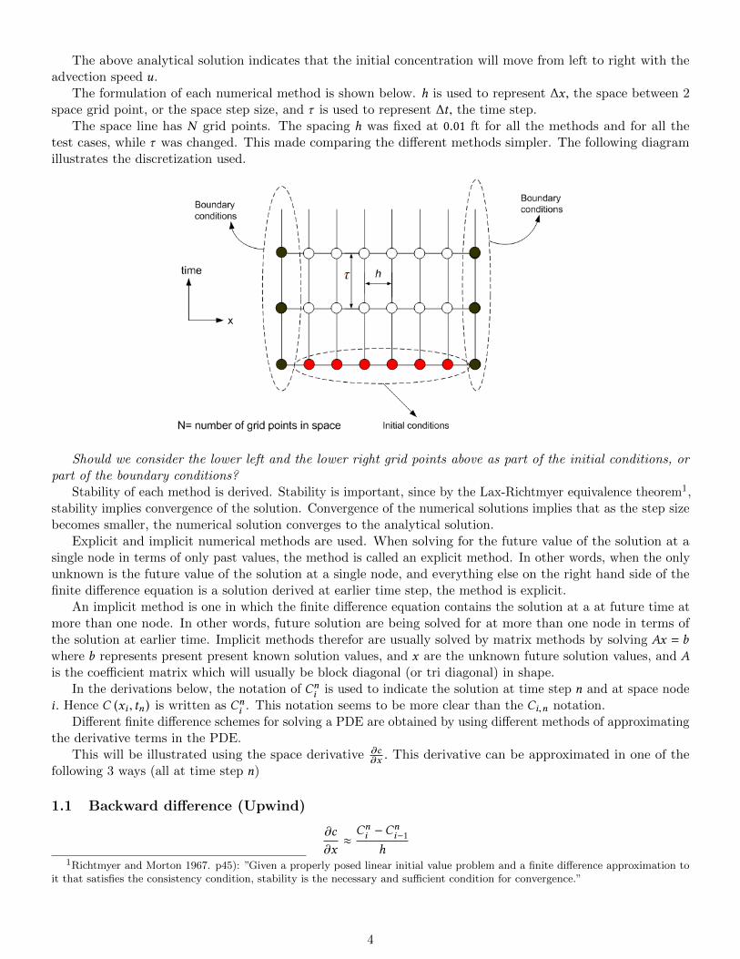
The formulation of each numerical method is shown below. h is used to represent ∆x , the space between 2space grid point, or the space step size, and τ is used to represent ∆t , the time step.

The space line has N grid points. The spacing h was fixed at 0.01 ft for all the methods and for all thetest cases, while τ was changed. This made comparing the different methods simpler. The following diagramillustrates the discretization used.

Should we consider the lower left and the lower right grid points above as part of the initial conditions, orpart of the boundary conditions?

Stability of each method is derived. Stability is important, since by the Lax-Richtmyer equivalence theorem1,stability implies convergence of the solution. Convergence of the numerical solutions implies that as the step sizebecomes smaller, the numerical solution converges to the analytical solution.

Explicit and implicit numerical methods are used. When solving for the future value of the solution at asingle node in terms of only past values, the method is called an explicit method. In other words, when the onlyunknown is the future value of the solution at a single node, and everything else on the right hand side of thefinite difference equation is a solution derived at earlier time step, the method is explicit.

An implicit method is one in which the finite difference equation contains the solution at a at future time atmore than one node. In other words, future solution are being solved for at more than one node in terms ofthe solution at earlier time. Implicit methods therefor are usually solved by matrix methods by solving Ax = bwhere b represents present present known solution values, and x are the unknown future solution values, and Ais the coefficient matrix which will usually be block diagonal (or tri diagonal) in shape.

In the derivations below, the notation of Cni is used to indicate the solution at time step n and at space node

i . Hence C (xi , tn ) is written as Cni . This notation seems to be more clear than the Ci,n notation.

Different finite difference schemes for solving a PDE are obtained by using different methods of approximatingthe derivative terms in the PDE.

This will be illustrated using the space derivative ∂c∂x . This derivative can be approximated in one of the

following 3 ways (all at time step n)

1.1 Backward difference (Upwind)

∂c

∂x≈Cni −C

ni−1

h1Richtmyer and Morton 1967. p45): ”Given a properly posed linear initial value problem and a finite difference approximation to

it that satisfies the consistency condition, stability is the necessary and sufficient condition for convergence.”

4

1.2 Forward difference (downwind)

∂c

∂x≈Cni+1 −C

ni

h

1.3 Center difference

∂c

∂x≈Cni+1 −C

ni−1

2h

The following are the derivation of a number of methods for solving the advection PDE obtained by usingthe above definitions for the derivative when applied to both space and time.

2 Numerical schemes

2.1 Explicit Methods

2.1.1 FTCS

With FTCS, the forward time derivative, and the centered space derivative are used. Hence the advection PDEcan be written as

Cn+1i −Cn

i

τ= −u

(Cni+1 −C

ni−1

2h

)(0)

Solving for Cn+1i results in

Cn+1i = Cn

i −uτ

2h

(Cni+1 −C

ni−1

)(1)

This method will be shown to be unconditionally unstable.

2.1.2 Downwind

Here, the forward time derivative for ∂C∂t is used and also the forward space derivative for ∂C∂x . This results in

Cn+1i −Cn

i

τ= −u

(Cni+1 −C

ni

h

)

Cn+1i = Cn

i −uτ

h

(Cni+1 −C

ni)

This method will be shown to be unconditionally unstable as well.

2.1.3 Upwind

Here, the forward time derivative for ∂C∂t is used, and the backward derivative for ∂C

∂x is used. This results in

Cn+1i −Cn

i

τ= −u

(Cni −C

ni−1

h

)

Cn+1i = Cn

i −uτ

h

(Cni −C

ni−1

)This will be shown to be stable if uτ

h ≤ 1

5

2.1.4 LAX

Looking at the FTCS eq (1) above, and shown below again

Cn+1i = Cn

i −uτ

2h

(Cni+1 −C

ni−1

)The term Cn

i above is replaced by its average valueCni+1+C

ni−1

2 to obtain the LAX method

Cn+1i =

12

(Cni+1 +C

ni−1

)−uτ

2h

(Cni+1 −C

ni−1

)(4)

This method will be shown to be stable if uτh ≤ 1

2.1.5 Lax-Wendroff

By using the second-order finite difference scheme for the time derivative, the method of Lax-Wendroff methodis obtained

Cn+1i = Cn

i −uτ

2h

(Cni+1 −C

ni−1

)+u2τ 2

2h2(Cni+1 +C

ni−1 − 2C

ni)

2.1.6 Leap-frog

In this method, the centered derivative is used for both time and space. This results in

Cn+1i −Cn−1

i

2τ= −u

(Cni+1 −C

ni−1

2h

)This method requires a special starting procedure due to the term Cn−1

i . Another scheme such as Lax can beused to kick start this method.

2.2 Implicit Methods

2.2.1 Implicit FTCS

Given the explicit FTCS derived above

Cn+1i −Cn

i

τ= −u

(Cni+1 −C

ni−1

2h

)The above is modified it by evaluating the space center derivative at time step n + 1 instead of at time step n,

this results in

Cn+1i −Cn

i

τ= −u

(Cn+1i+1 −C

n+1i−1

2h

)(5A)

Hence

Cn+1i +

uτ

2hCn+1i+1 −

uτ

2hCn+1i−1 = C

ni (5B)

Writing it in matrix form, first letting α = uτ2h results in

6

1 0 0 0 · · · 0 0

−α 1 α 0 · · · 0 0

0 −α 1 α · · · 0 0

0 0 −α 1 α · · · 0...

0 0 0 0 0 0 1

Cn+10

Cn+11

Cn+12

Cn+13...

Cn+1N−1

=

Cn0

Cn1

Cn2

Cn3...

CnN−1

Where N is the number of space grid points.The above is written as

Ax = b

Solving for x , which represents the solution at time step n+ 1 or at time t = (n + 1) τ . b represents the currentsolution at time step n, and A is the matrix of the coefficients shown above.

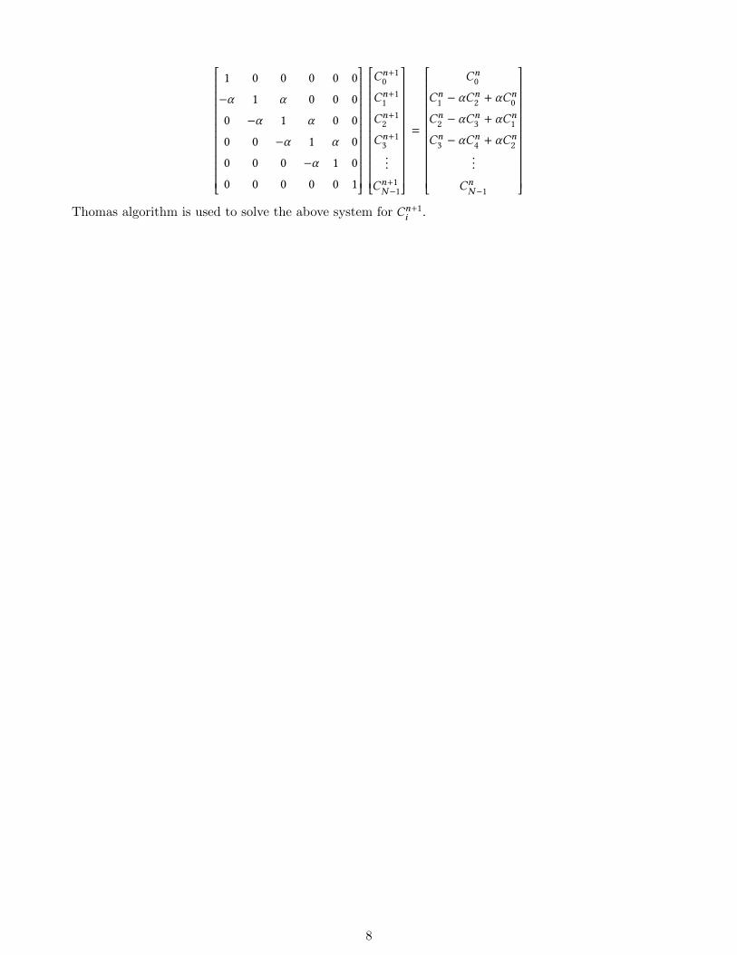
Due to the form of the A matrix, (Called tri diagonal, or Block diagonal), an algorithm that takes advantagesof this form is used. This is called the Thomas algorithm. This greatly speeds up the solution. If we had used ageneral algorithm to solve this system such as the Gauss elimination method, it would have been much slower,making the implicit method not practical to use. (Some tests on the same data showed the Thomas algorithm tobe 50 times faster than Gaussian elimination).

2.2.2 Wendrof

This method uses center difference for the derivative around the space step(i + 1

2

)h and the time step

(n + 1

2

)τ

This leads to the following scheme(1 −

uτ

h

)Cn+1i +

(1 +

uτ

h

)Cn+1i+1 =

(1 +

uτ

h

)Cni +

(1 −

uτ

h

)Cni+1

This can also be solved using similar matrix method to that used for the implicit FTCS. This method is notused in this report.

2.2.3 Crank-Nicolson

By taking the average of the explicit FTCS and the implicit FTCS formulations (shown again below), the C-Nscheme is derived

Cn+1i −Cn

i

τ= −u

(Cni+1 −C

ni−1

2h

)Cn+1i −Cn

i

τ= −u

(Cn+1i+1 −C

n+1i−1

2h

)Taking the average of the above results in

Cn+1i −Cn

i

τ= −

u

2

(Cni+1 −C

ni−1

2h

)−u

2

(Cn+1i+1 −C

n+1i−1

2h

)

Cn+1i +

uτ

4hCn+1i+1 −

uτ

4hCn+1i−1 = C

ni −

uτ

4hCni+1 +

uτ

4hCni−1

Now the system Ax = b is setup to solve for future values as follows. Let α = uτ4h , the system can be written as

7

1 0 0 0 0 0

−α 1 α 0 0 0

0 −α 1 α 0 0

0 0 −α 1 α 0

0 0 0 −α 1 0

0 0 0 0 0 1

Cn+10

Cn+11

Cn+12

Cn+13...

Cn+1N−1

=

Cn0

Cn1 − αC

n2 + αC

n0

Cn2 − αC

n3 + αC

n1

Cn3 − αC

n4 + αC

n2

...

CnN−1

Thomas algorithm is used to solve the above system for Cn+1

i .

8

3 Stability analysis

A numerical solution is stable if the ”energy content” remain below some limiting value no matter how long thesolution is integrated. In essence, this means that the solution does not ’blow up’ after some time. This can becalled BIBO stability (Bounded In Bounded Out).

Hence one way to analyze the stability of the numerical solution is to determine an expression that relatesthe amplitude of the solution between 2 time steps, and to determine if this ratio remain less than or equal to aunity as more and more time steps are taken.

This type of analysis is called Von Neumann stability analysis for numerical methods.The analysis is based of finding an expression for the magnification factor of the wave amplitude at each

step. The solution will be stable if this magnification factor is less than one.Let the magnification factor be ξ . The numerical scheme is stable iff

��ζ �� ≤ 1

The Courant–Friedrichs–Lewy (CFL) criteria for stability says that

��ζ �� ≤ 1⇔��uτ

h

�� ≤ 1

Where u,h, and τ are as defined above: u is the wave speed, h = ∆x and τ = ∆t .The number uτ

h is also called the courant number .Some numerical methods will be shown to be unconditionally unstable (such as explicit FTCS and the

explicit upwind). This means that even if courant number was ≤ 1, the numerical solutions will eventuallybecome unstable.

Some explicit methods such as LAX, are conditionally stable if the courant number was ≤ 1.Implicit methods are unconditionally stable, hence courant number is not used for these methods. However,

this does not mean one can take as large step as one wants with the implicit methods, since accuracy will beaffected even if the solution remain stable.

Hence, the best numerical scheme is one in which the largest step size can be taken, with the least amount ofinaccuracy in the numerical solution while remaining stable.

For numerical scheme that are conditionally stable, it can be seen from the CFL condition that for a fixedspeed u and fixed h, the maximum time step that can be taken is given by

τmax ≤h

u

It can be immediately seen from above, that for the case when the advection speed is varying and is afunction of time such as the case when u (t ) = t

20 implying that the speed is increasing with time, then when

using a fixed time step τ it will eventually become larger than hu and the numerical scheme will be unstable. This

is because as u (t ) is becoming larger and larger, while h is fixed, the term hu will become smaller and smaller.

Hence to keep the courant number uτh ≤ 1 , the time step taken must remain less than h

u , hence using a fixedtime step with increasing u will eventually lead to instability.

This will affect the explicit methods that are conditionally stable such as the LAX method, since the Laxmethod is explicit and depends on satisfying the CFL all the time for its stability. Implicit methods are stablefor any time step.

In the following we derive the details of the stability analysis and use Von Neumann analysis to derive anexpression for the amplification factor ζ for different numerical schemes.

So to summarize:

1. Explicit FTCS is unconditionally unstable.

2. Explicit LAX is stable if uτh ≤ 1, or in other words, τmax ≤

hu

3. Implicit FTCS and C-R are stable for all τ

9

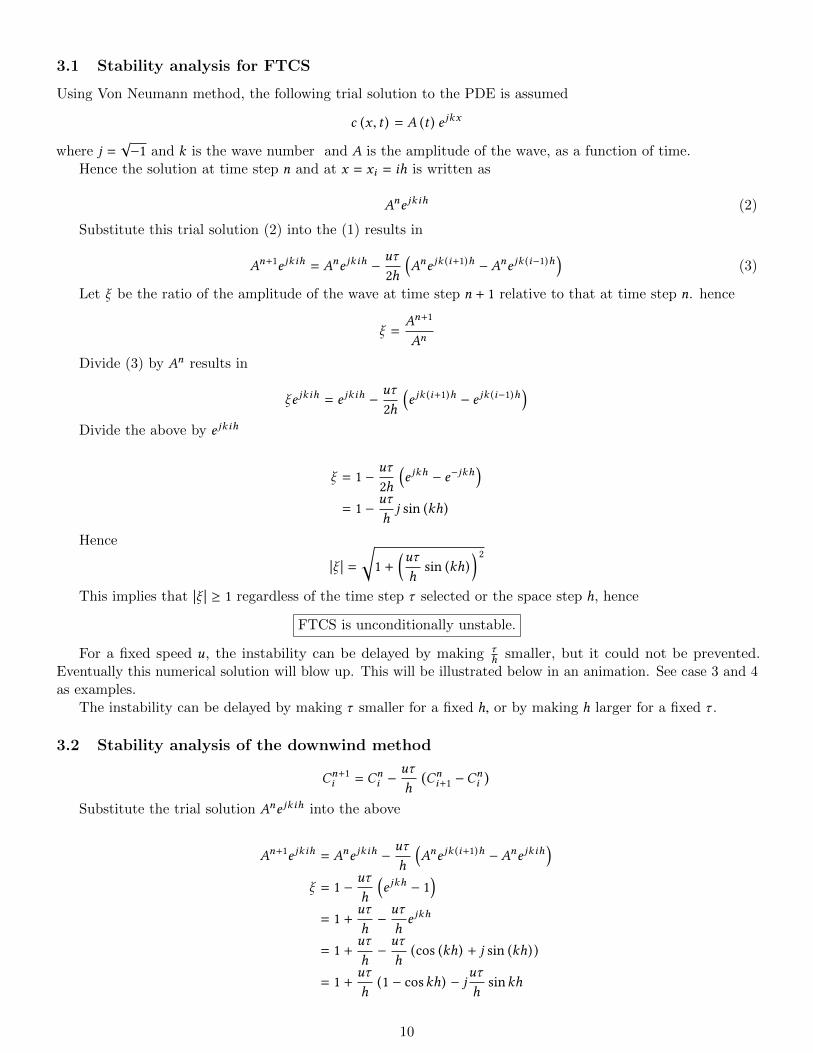
3.1 Stability analysis for FTCS

Using Von Neumann method, the following trial solution to the PDE is assumed

c (x , t ) = A (t ) e jkx

where j =√−1 and k is the wave number and A is the amplitude of the wave, as a function of time.

Hence the solution at time step n and at x = xi = ih is written as

Ane jkih (2)

Substitute this trial solution (2) into the (1) results in

An+1e jkih = Ane jkih −uτ

2h

(Ane jk (i+1)h −Ane jk (i−1)h

)(3)

Let ξ be the ratio of the amplitude of the wave at time step n + 1 relative to that at time step n. hence

ξ =An+1

An

Divide (3) by An results in

ξe jkih = e jkih −uτ

2h

(e jk (i+1)h − e jk (i−1)h

)Divide the above by e jkih

ξ = 1 −uτ

2h

(e jkh − e−jkh

)= 1 −

uτ

hj sin (kh)

Hence

��ξ �� =√1 +

(uτh

sin (kh)) 2

This implies that ��ξ �� ≥ 1 regardless of the time step τ selected or the space step h, hence

FTCS is unconditionally unstable.

For a fixed speed u, the instability can be delayed by making τh smaller, but it could not be prevented.

Eventually this numerical solution will blow up. This will be illustrated below in an animation. See case 3 and 4as examples.

The instability can be delayed by making τ smaller for a fixed h, or by making h larger for a fixed τ .

3.2 Stability analysis of the downwind method

Cn+1i = Cn

i −uτ

h

(Cni+1 −C

ni)

Substitute the trial solution Ane jkih into the above


h

(Ane jk (i+1)h −Ane jkih

)ξ = 1 −

uτ

h

(e jkh − 1

)= 1 +

uτ

h−uτ

he jkh

= 1 +uτ

h−uτ

h(cos (kh) + j sin (kh) )

= 1 +uτ

h(1 − coskh) − j

uτ

hsinkh

10

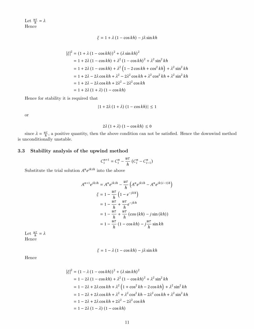
Let uτh = λ

Hence

ξ = 1 + λ (1 − coskh) − jλ sinkh

��ξ ��2 = (1 + λ (1 − coskh) )2 + (λ sinkh)2

= 1 + 2λ (1 − coskh) + λ2 (1 − coskh)2 + λ2 sin2 kh

= 1 + 2λ (1 − coskh) + λ2(1 − 2 coskh + cos2 kh

)+ λ2 sin2 kh

= 1 + 2λ − 2λ coskh + λ2 − 2λ2 coskh + λ2 cos2 kh + λ2 sin2 kh

= 1 + 2λ − 2λ coskh + 2λ2 − 2λ2 coskh

= 1 + 2λ (1 + λ) (1 − coskh)

Hence for stability it is required that

|1 + 2λ (1 + λ) (1 − coskh) | ≤ 1

or

2λ (1 + λ) (1 − coskh) ≤ 0

since λ = uτh , a positive quantity, then the above condition can not be satisfied. Hence the downwind method

is unconditionally unstable.

3.3 Stability analysis of the upwind method

Cn+1i = Cn

i −uτ

h

(Cni −C

ni−1

)Substitute the trial solution Ane jkih into the above


h

(Ane jkih −Ane jk (i−1)h

)ξ = 1 −

uτ

h

(1 − e−jkh

)= 1 −

uτ

h+uτ

he−jkh

= 1 −uτ

h+uτ

h(cos (kh) − j sin (kh) )

= 1 −uτ

h(1 − coskh) − j

uτ

hsinkh

Let uτh = λ

Hence

ξ = 1 − λ (1 − coskh) − jλ sinkh

Hence

��ξ ��2 = (1 − λ (1 − coskh) )2 + (λ sinkh)2

= 1 − 2λ (1 − coskh) + λ2 (1 − coskh)2 + λ2 sin2 kh

= 1 − 2λ + 2λ coskh + λ2(1 + cos2 kh − 2 coskh

)+ λ2 sin2 kh

= 1 − 2λ + 2λ coskh + λ2 + λ2 cos2 kh − 2λ2 coskh + λ2 sin2 kh

= 1 − 2λ + 2λ coskh + 2λ2 − 2λ2 coskh

= 1 − 2λ (1 − λ) (1 − coskh)

11

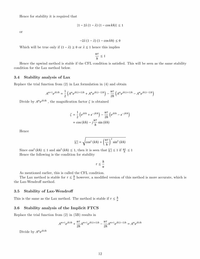
Hence for stability it is required that

|1 − 2λ (1 − λ) (1 − coskh) | ≤ 1

or

−2λ (1 − λ) (1 − coskh) ≤ 0

Which will be true only if (1 − λ) ≥ 0 or λ ≤ 1 hence this implies

uτ

h≤ 1

Hence the upwind method is stable if the CFL condition is satisfied. This will be seen as the same stabilitycondition for the Lax method below.

3.4 Stability analysis of Lax

Replace the trial function from (2) in Lax formulation in (4) and obtain

An+1e jkih =12

(Ane jk (i+1)h +Ane jk (i−1)h

)−uτ

2h

(Ane jk (i+1)h −Ane jk (i−1)h

)Divide by Ane jkih , the magnification factor ζ is obtained

ζ =12

(e jkh + e−jkh

)−uτ

2h

(e jkh − e−jkh

)= cos (kh) − j

uτ

hsin (kh)

Hence

��ζ �� =√cos2 (kh) +

(uτh

) 2sin2 (kh)

Since cos2 (kh) ≤ 1 and sin2 (kh) ≤ 1, then it is seen that ��ζ �� ≤ 1 if uτh ≤ 1

Hence the following is the condition for stability

τ ≤h

u

As mentioned earlier, this is called the CFL condition.The Lax method is stable for τ ≤ h

u however, a modified version of this method is more accurate, which isthe Lax-Wendroff method.

3.5 Stability of Lax-Wendroff

This is the same as the Lax method. The method is stable if τ ≤ hu

3.6 Stability analysis of the Implicit FTCS

Replace the trial function from (2) in (5B) results in

An+1e jkih +uτ

2hAn+1e jk (i+1)h −

uτ

2hAn+1e jk (i−1)h = Ane jkih

Divide by Ane jkih

12

ξ +uτ

2hξe jkh −

uτ

2hξe−jkh = 1

ξ(1 +

uτ

2he jkh −

uτ

2he−jkh

)= 1

ξ(1 + j

uτ

hsin (kh)

)= 1

ξ =1

1 + j uτh sin (kh)=

1 − j uτh sin (kh)

1 + uτh sin (kh)

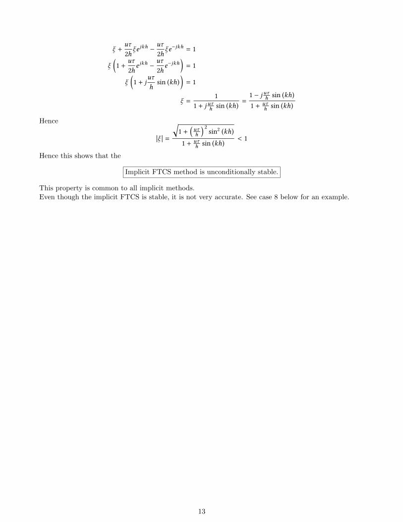
Hence

��ξ �� =

√1 +

(uτh

) 2sin2 (kh)

1 + uτh sin (kh)

< 1

Hence this shows that the

Implicit FTCS method is unconditionally stable.

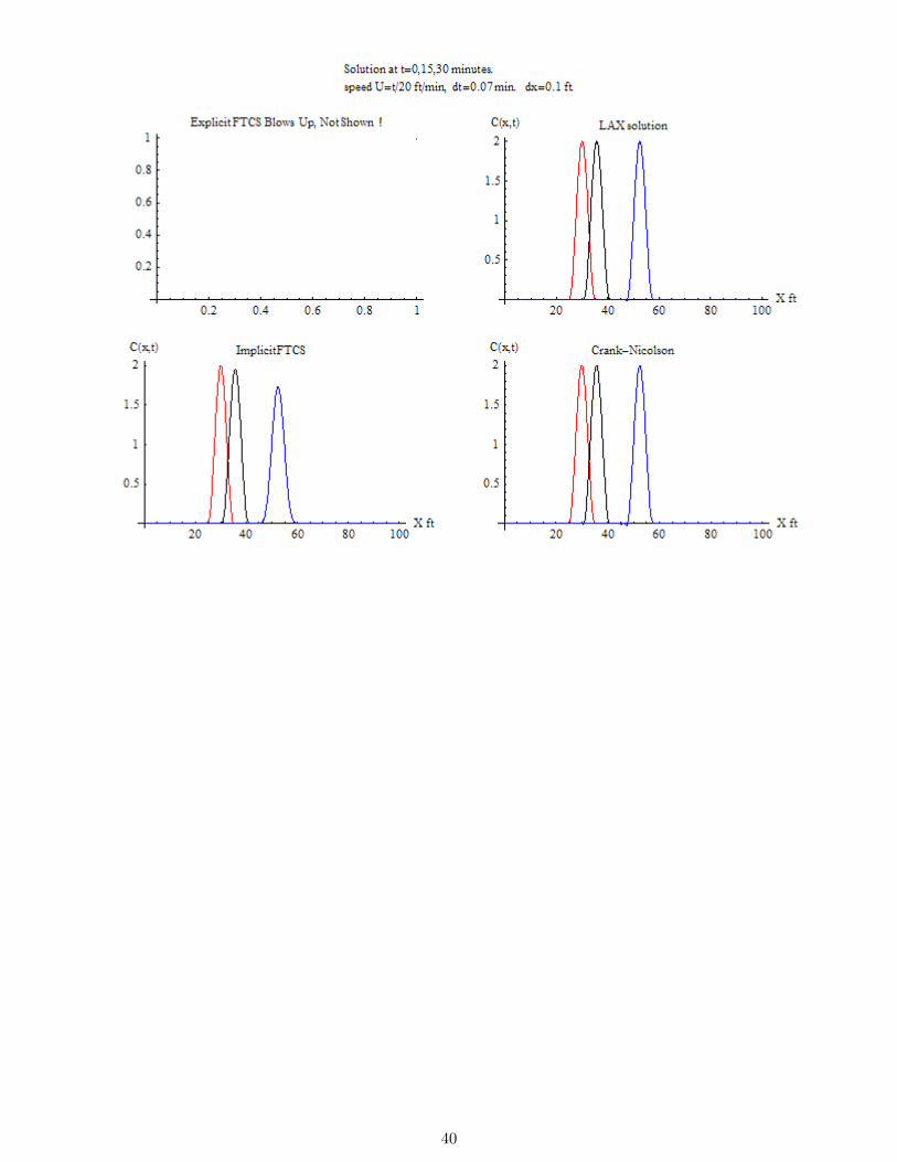
This property is common to all implicit methods.Even though the implicit FTCS is stable, it is not very accurate. See case 8 below for an example.

13

4 Solution Results and Output

For the Fortran implementation, the following methods are implemented. The explicit FTCS, Explicit Lax,Implicit FTCS, and Implicit Crank-Nicolson.

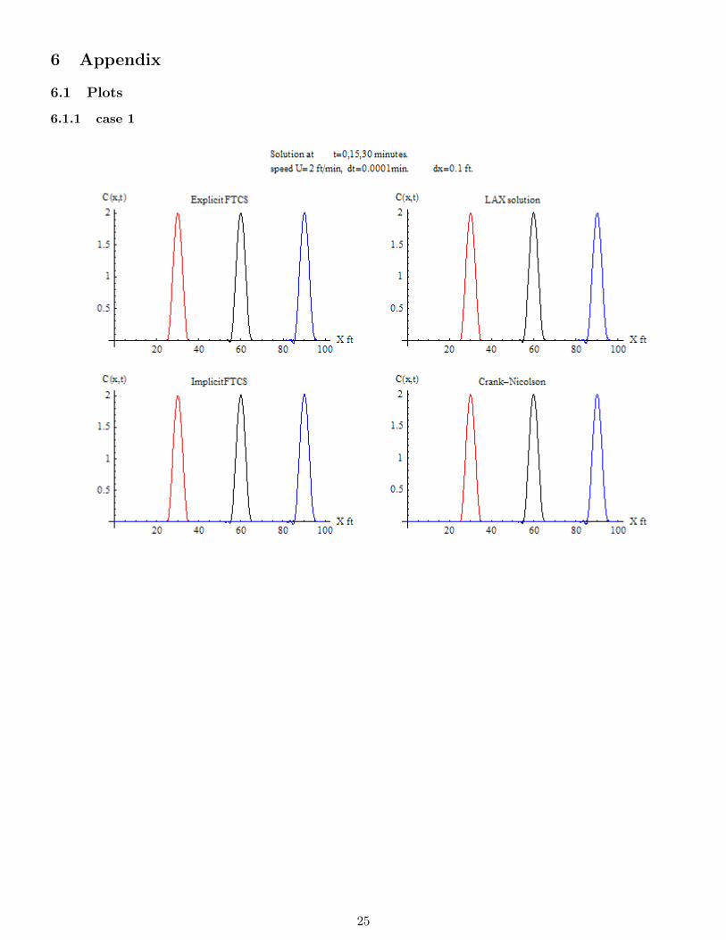
For each method, the following was generated

1. CPU time used for the run.

2. snap shot of the solution at t = 0, t = 15, and t = 30 minutes.

3. RMSE between the numerical solution and the analytical solution.

4. Animation of the numerical solution. The animation was done by taking snapshots of the solution atregular intervals in Fortran. These were saved to disk. Then Mathematica was used to generate theanimation and the plots.

To compare the stability and accuracy of the methods, the time step was changed (increased) and a new runwas made. 8 different values of time steps are used. So there are 8 tests cases. These 8 test cases were run forboth fixed speed

(u = 2 ft/min

)and for u = t

20 ft/min.This table below summarizes these cases. The appendix contains all the plots. The animations are added as

HTML links.

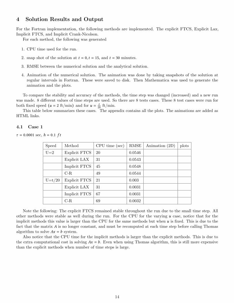
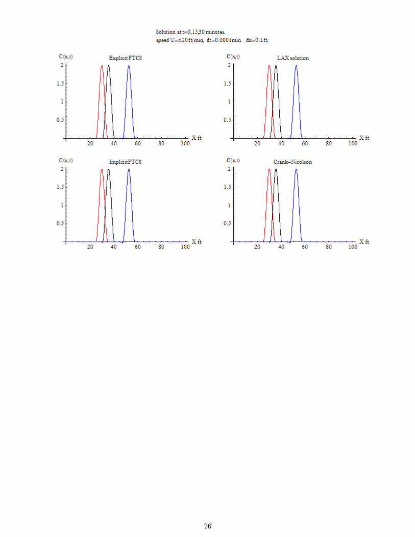
4.1 Case 1

τ = 0.0001 sec, h = 0.1 f t

Speed Method CPU time (sec) RMSE Animation (2D) plots

U=2 Explicit FTCS 20 0.0546

Explicit LAX 31 0.0543

Implicit FTCS 45 0.0548

C-R 49 0.0544

U=t/20 Explicit FTCS 21 0.003

Explicit LAX 31 0.0031


C-R 69 0.0032

Note the following: The explicit FTCS remained stable throughout the run due to the small time step. Allother methods were stable as well during the run. For the CPU for the varying u case, notice that for theimplicit methods this value is larger than the CPU for the same methods but when u is fixed. This is due to thefact that the matrix A is no longer constant, and must be recomputed at each time step before calling Thomasalgorithm to solve Ax = b system.

Also notice that the CPU time for the implicit methods is larger than the explicit methods. This is due tothe extra computational cost in solving Ax = b. Even when using Thomas algorithm, this is still more expensivethan the explicit methods when number of time steps is large.

14

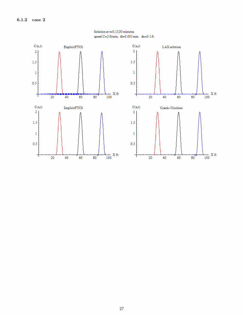
4.2 Case 2

τ = 0.001 sec, h = 0.1 f t


U=2 Explicit FTCS 2.42 0.01264

Explicit LAX 3.48 0.0057

Implicit FTCS 4.7 0.00742

C-R 4.9 0.00575

U=t/20 Explicit FTCS 2.5 0.00352



C-R 7.5 0.0033

The explicit FTCS is stable for most of the run, near the end it is starting to be become unstable.Notice that around 26 minutes that ”bubbles” are starting to show up in the numerical solution downstream.

This is a characteristic of how this method becomes unstable.This will be more clear in the next test cases when the time step is made larger. For the varying speed case,

the explicit method using the same time step remained stable during the whole 30 minutes. This is because theaverage speed was less than 2 ft/min, hence the mass did not have to travel as long a distance as with fixedspeed of u = 2, and so the instability did not show up. Mathematically this can be explained by looking at theterm uτ

h , hence for smaller u, the courant number is smaller. Notice also the RMSE is smaller for variable speedcompared to fixed speed. Again this is related to the smaller average speed making the courant number smaller.

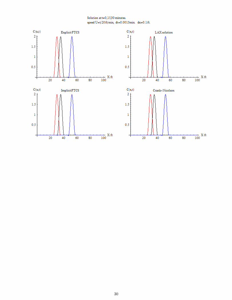
4.3 Case 3

In this case, we slightly make the time step longer than before. We start to see the instability of FTCS.τ = 0.0013 sec, h = 0.1 ft, uτh = 0.026 ≤ 1 for fixed u





C-R 3.9 0.01128




C-R 6 0.00331

For explicit FTCS, The solution now starting to show instability at 25 minutes. Lax remained stable sinceCFL is satisfied. Explicit FTCS is becoming less accurate as well. Explicit Lax is most accurate at this timestep.

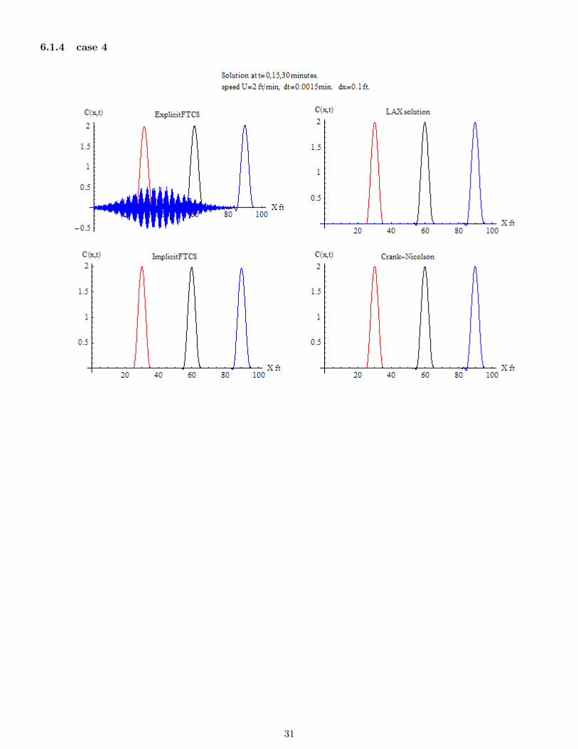
4.4 Case 4

In this case, we slightly make the time step even longer than before. Now FTCS becomes more unstable.τ = 0.0015 sec, h = 0.1 ft, uτh = 0.03 ≤ 1.

15





C-R 3.45 0.00565



Implicit FTCS 4,73 0.00358

C-R 5 0.003373

FTCS Instability starts at around 20 minutes. LAX remained stable since CFL is satisfied. Lax remainedthe most accurate at this time step. It accuracy actually improved as the time step became larger.

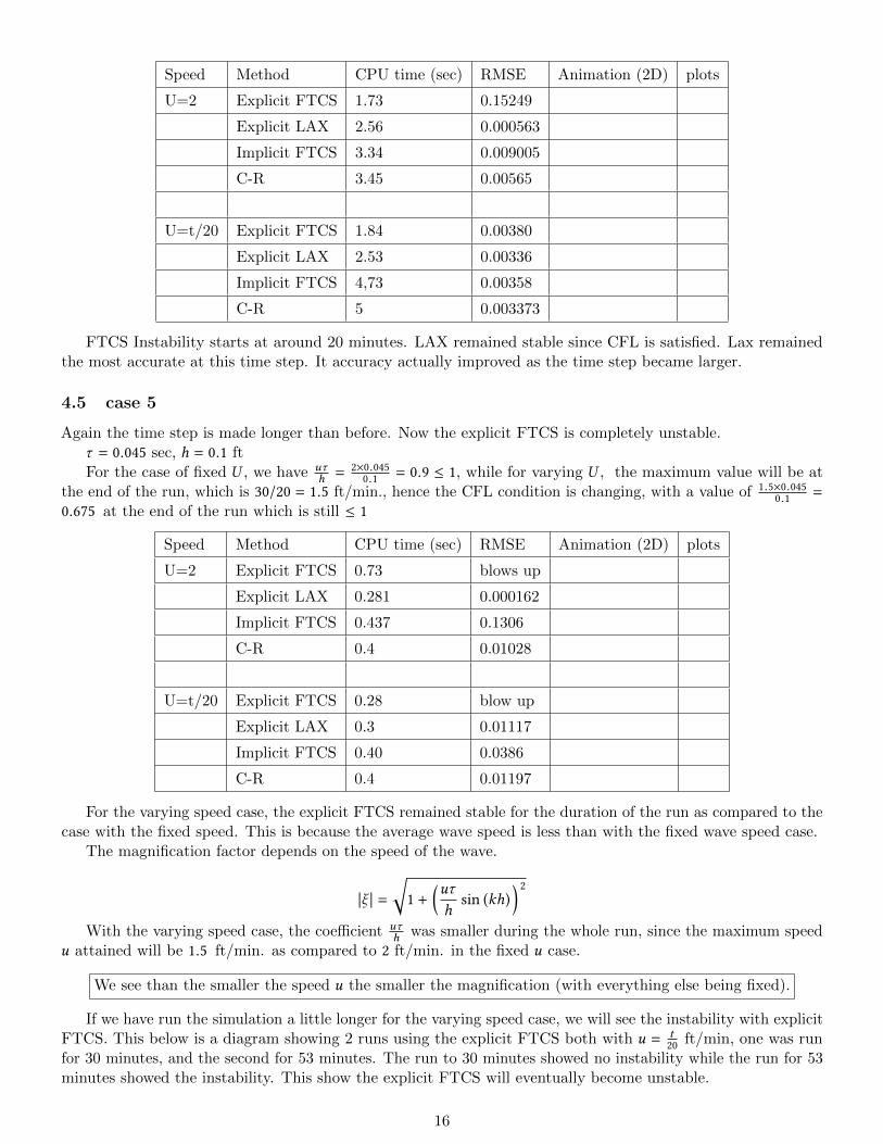
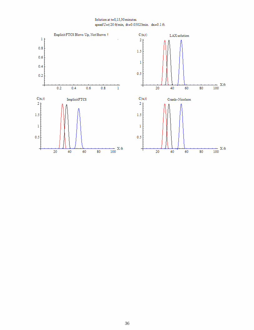
4.5 case 5

Again the time step is made longer than before. Now the explicit FTCS is completely unstable.τ = 0.045 sec, h = 0.1 ftFor the case of fixed U , we have uτ

h =2×0.045

0.1 = 0.9 ≤ 1, while for varying U , the maximum value will be atthe end of the run, which is 30/20 = 1.5 ft/min., hence the CFL condition is changing, with a value of 1.5×0.045

0.1 =

0.675 at the end of the run which is still ≤ 1


U=2 Explicit FTCS 0.73 blows up



C-R 0.4 0.01028

U=t/20 Explicit FTCS 0.28 blow up



C-R 0.4 0.01197

For the varying speed case, the explicit FTCS remained stable for the duration of the run as compared to thecase with the fixed speed. This is because the average wave speed is less than with the fixed wave speed case.

The magnification factor depends on the speed of the wave.

��ξ �� =√1 +

(uτh

sin (kh)) 2

With the varying speed case, the coefficient uτh was smaller during the whole run, since the maximum speed

u attained will be 1.5 ft/min. as compared to 2 ft/min. in the fixed u case.

We see than the smaller the speed u the smaller the magnification (with everything else being fixed).

If we have run the simulation a little longer for the varying speed case, we will see the instability with explicitFTCS. This below is a diagram showing 2 runs using the explicit FTCS both with u = t

20 ft/min, one was runfor 30 minutes, and the second for 53 minutes. The run to 30 minutes showed no instability while the run for 53minutes showed the instability. This show the explicit FTCS will eventually become unstable.

16

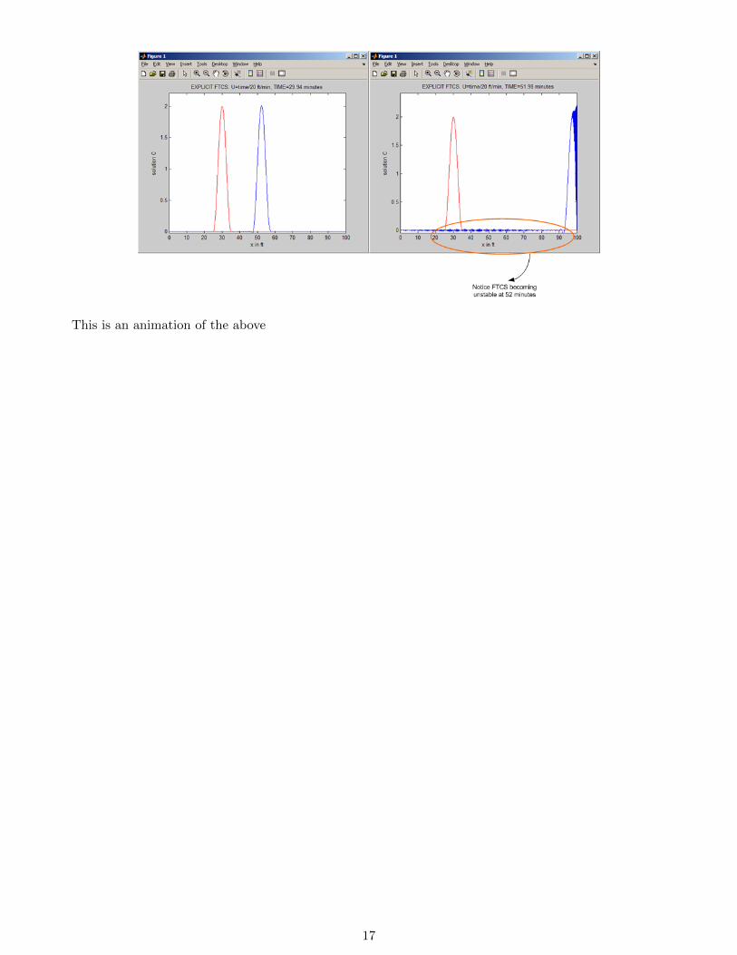
This is an animation of the above

17

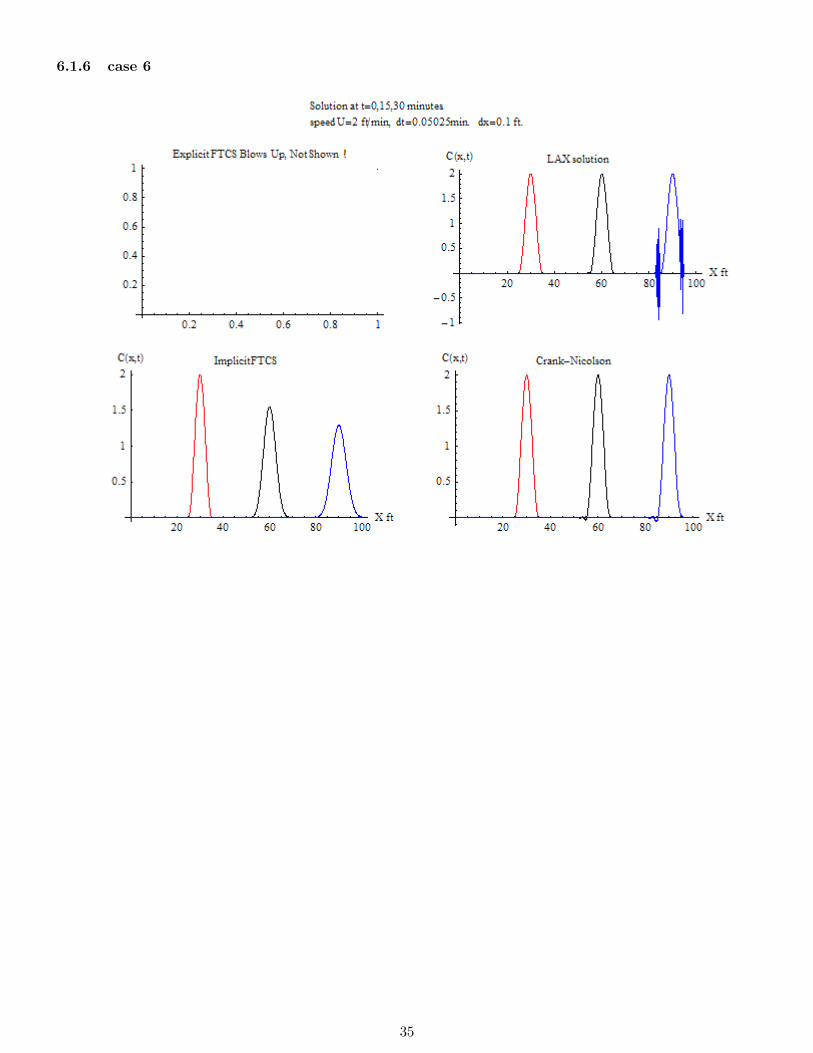
4.6 case 6

In this case, the time step is increased so that uτh is just above the CFL condition.

Notice now that the Explicit LAX method become unstable as expected. The other implicit methods remainstable. the explicit FTCS method now is completely unstable. The implicit FTCS method is starting to becomeless accurate.

τ = 0.05025 sec, h = 0.1 ft, uτh =2×0.05025

0.1 = 1. 005 > 1


U=2 Explicit FTCS 0.7 blows up N/A blows up



C-R 0.468 0.01104

U=t/20 Explicit FTCS 0.28 blows up N/A blows up



C-R 0.56 0.01317

Notice that explicit LAX takes much less CPU than any other method.

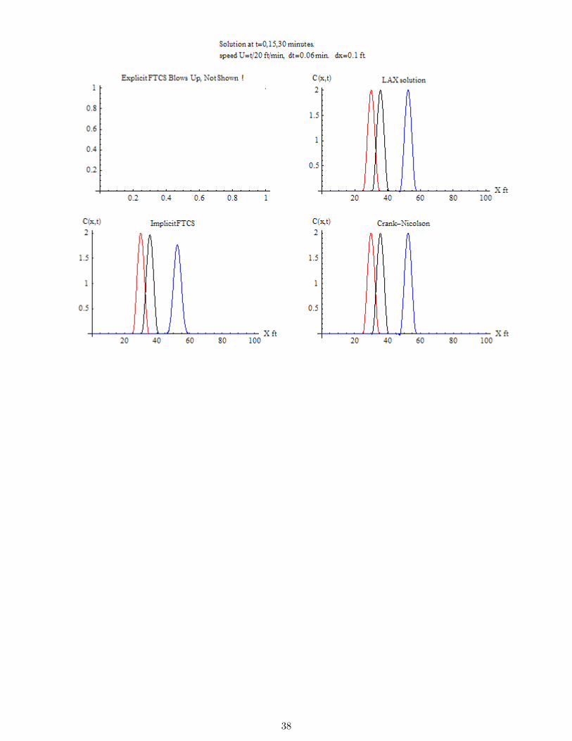
4.7 case 7

τ = 0.06 sec, h = 0.1 ft, uτh =2×0.060.1 = 1. 2 > 1



Explicit LAX 0.9 blows up


C-R 0.41 0.01244




C-R 0.36 0.01525

Notice that the CPU for the implicit method when speed is fixed is now higher than the CPU for the explicitmethods. This can be explained as follows: since the time step now is larger than before, the number of times tosolve Ax = b has been reduced. This made the implicit methods faster.

This implies that

Using a relatively large time step, implicit methods become faster than the explicit methods.

18

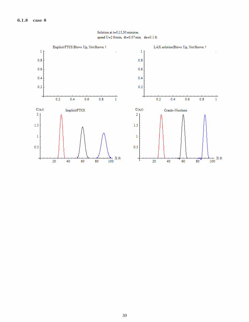
4.8 case 8

τ = 0.07 sec, h = 0.1 ft, uτh =2×0.070.1 = 1. 4 > 1



Explicit LAX 0.89 blows up


C-R 0.36 0.01403




C-R 0.312 0.0174

19

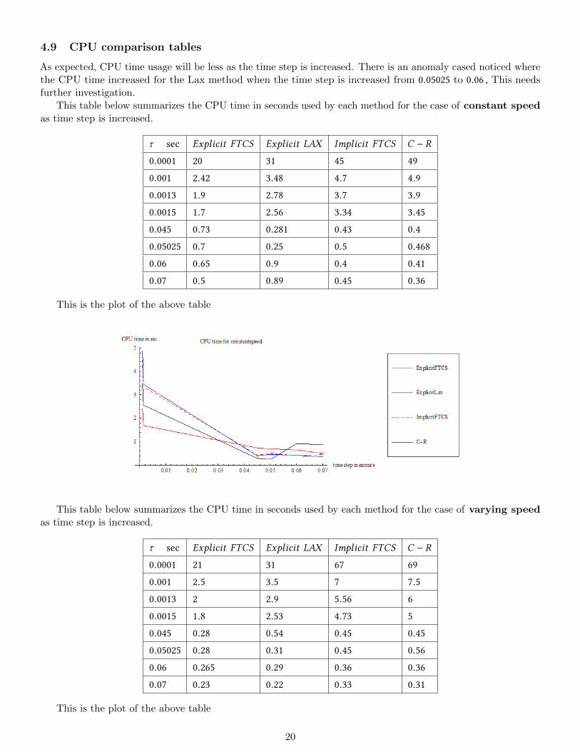
4.9 CPU comparison tables

As expected, CPU time usage will be less as the time step is increased. There is an anomaly cased noticed wherethe CPU time increased for the Lax method when the time step is increased from 0.05025 to 0.06 , This needsfurther investigation.

This table below summarizes the CPU time in seconds used by each method for the case of constant speedas time step is increased.

τ sec Explicit FTCS Explicit LAX Implicit FTCS C − R

0.0001 20 31 45 49

0.001 2.42 3.48 4.7 4.9

0.0013 1.9 2.78 3.7 3.9

0.0015 1.7 2.56 3.34 3.45

0.045 0.73 0.281 0.43 0.4

0.05025 0.7 0.25 0.5 0.468

0.06 0.65 0.9 0.4 0.41

0.07 0.5 0.89 0.45 0.36

This is the plot of the above table

This table below summarizes the CPU time in seconds used by each method for the case of varying speedas time step is increased.

τ sec Explicit FTCS Explicit LAX Implicit FTCS C − R

0.0001 21 31 67 69

0.001 2.5 3.5 7 7.5

0.0013 2 2.9 5.56 6

0.0015 1.8 2.53 4.73 5

0.045 0.28 0.54 0.45 0.45

0.05025 0.28 0.31 0.45 0.56

0.06 0.265 0.29 0.36 0.36

0.07 0.23 0.22 0.33 0.31

This is the plot of the above table

20

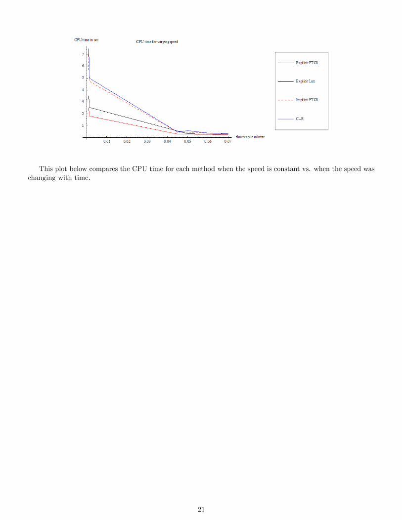
This plot below compares the CPU time for each method when the speed is constant vs. when the speed waschanging with time.

21

4.10 Accuracy comparison tables

This table below summarizes the RMS error from each numerical method as a function of changing the timestep size. This is for case of constant speed.

time step Explicit FTCS Explicit LAX Implicit FTCS C − R

0.0001 0.0546 0.0543 0.0548 0.0544

0.001 0.01264 0.0057 0.00742 0.00575

0.0013 0.0494 0.01125 0.01245 0.00128

0.0015 0.15249 0.00056 0.009 0.0056

0.045 blows up 0.000162 0.1306 0.01028

0.05025 blows up 0.1006 0.1394 0.011

0.06 blows up blows up 0.1531 0.01244

0.07 blows up blows up 0.1653 0.01403

Notice that the Lax method became more accurate when the time step was increased from 0.0001 to 0.04seconds, then it starts to become less accurate as time step is increased. This is counter intuitive to what onecan expect. It will be interesting to investigate this further to obtain a mathematical explanation for this strangephenomena.

The accuracy of the implicit FTCS, and C-R also increased slightly as the time step became larger from0.0001 to 0.0015, then the implicit FTCS became worst in terms of accuracy as the time step increased.

C-R method accuracy did not deteriorate as much with increasing the time step. This shows the C-R schemeto be more robust.

This table below summarizes the RMS error from each numerical method as a function of changing the timestep size. This is for case of changing speed.

time step Explicit FTCS Explicit LAX Implicit FTCS C − R

0.0001 0.003 0.003 0.003 0.0030

0.001 0.00352 0.00329 0.0033 0.0033

0.0013 0.00365 0.00331 0.00346 0.0033

0.0015 0.0038 0.00336 0.0035 0.00337

0.045 blows up 0.01117 0.0386 0.0119

0.05025 blows up 0.04385 0.0428 0.01317

0.06 blows up 0.01389 0.0493 0.01525

0.07 blows up 0.01564 0.0557 0.0174

The effect of having the speed defined as µ = t20 is to delay instability for the explicit methods as time step is

increased. Notice also here the case where the Lax method became more accurate as the time step is increasedfrom 0.0001 to 0.0015.

23

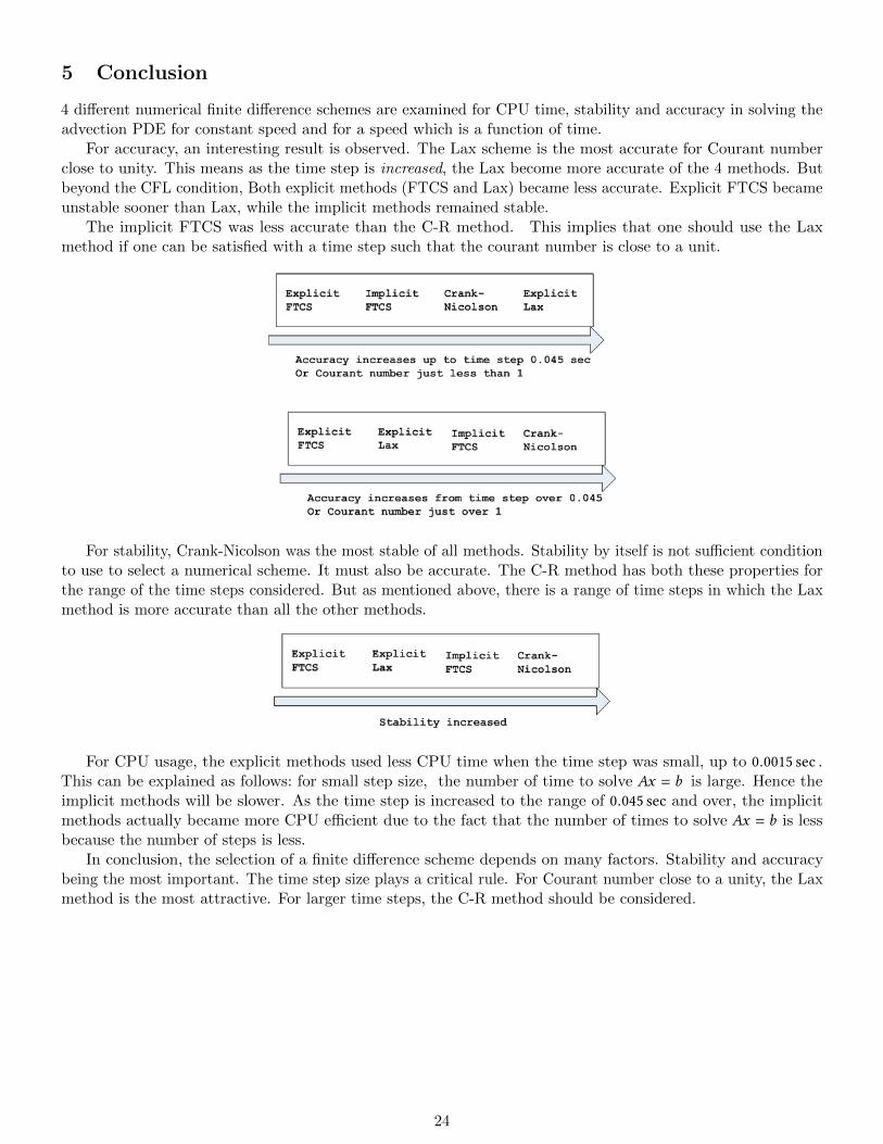
5 Conclusion

4 different numerical finite difference schemes are examined for CPU time, stability and accuracy in solving theadvection PDE for constant speed and for a speed which is a function of time.

For accuracy, an interesting result is observed. The Lax scheme is the most accurate for Courant numberclose to unity. This means as the time step is increased, the Lax become more accurate of the 4 methods. Butbeyond the CFL condition, Both explicit methods (FTCS and Lax) became less accurate. Explicit FTCS becameunstable sooner than Lax, while the implicit methods remained stable.

The implicit FTCS was less accurate than the C-R method. This implies that one should use the Laxmethod if one can be satisfied with a time step such that the courant number is close to a unit.

For stability, Crank-Nicolson was the most stable of all methods. Stability by itself is not sufficient conditionto use to select a numerical scheme. It must also be accurate. The C-R method has both these properties forthe range of the time steps considered. But as mentioned above, there is a range of time steps in which the Laxmethod is more accurate than all the other methods.

For CPU usage, the explicit methods used less CPU time when the time step was small, up to 0.0015 sec .This can be explained as follows: for small step size, the number of time to solve Ax = b is large. Hence theimplicit methods will be slower. As the time step is increased to the range of 0.045 sec and over, the implicitmethods actually became more CPU efficient due to the fact that the number of times to solve Ax = b is lessbecause the number of steps is less.

In conclusion, the selection of a finite difference scheme depends on many factors. Stability and accuracybeing the most important. The time step size plays a critical rule. For Courant number close to a unity, the Laxmethod is the most attractive. For larger time steps, the C-R method should be considered.

24

6 Appendix

6.1 Plots

6.1.1 case 1

25

6.1.2 case 2

27

6.1.3 case 3

29

6.1.4 case 4

31

6.1.5 case 5

33

6.1.6 case 6

35

6.1.7 case 7

37

6.1.8 case 8

39

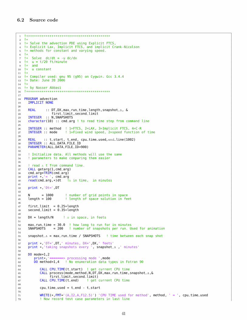
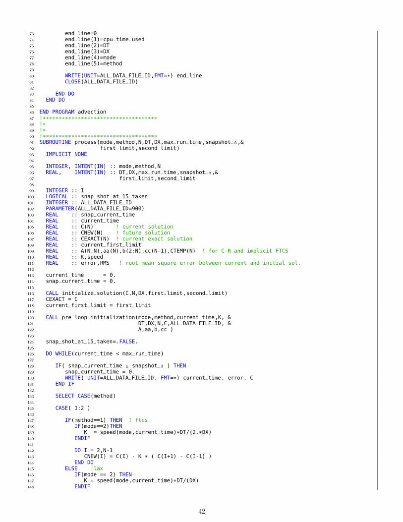
6.2 Source code

1 !*******************************************2 !*3 !* Solve the advection PDE using Explicit FTCS,4 !* Explicit Lax, Implicit FTCS, and implicit Crank-Nicolson5 !* methods for constant and varying speed.6 !*7 !* Solve dc/dt = -u dc/dx8 !* u = t/20 ft/minute9 !* and

10 !* u constant11 !*12 !* Compiler used: gnu 95 (g95) on Cygwin. Gcc 3.4.413 !* Date: June 20 200614 !*15 !* by Nasser Abbasi16 !*******************************************17

18 PROGRAM advection19 IMPLICIT NONE20

21 REAL :: DT,DX,max_run_time,length,snapshot_∆, &22 first_limit,second_limit23 INTEGER :: N,SNAPSHOTS24 character(10) :: cmd_arg ! to read time step from command line25

26 INTEGER :: method ! 1=FTCS, 2=LAX, 3=Implicit FTCS, 4=C-R27 INTEGER :: mode ! 1=Fixed wind speed, 2=speed function of time28

29 REAL :: t_start, t_end, cpu_time_used,end_line(1002)30 INTEGER :: ALL_DATA_FILE_ID31 PARAMETER(ALL_DATA_FILE_ID=900)32

33 ! Initialize data. All methods will use the same34 ! parameters to make comparing them easier35

36 ! read ∆ t from command line.37 CALL getarg(1,cmd_arg)38 cmd_arg=TRIM(cmd_arg)39 print *,'= ', cmd_arg40 read(cmd_arg,*)dt !∆ in time, in minutes41

42 print *,'Dt=',DT43

44 N = 1000 ! number of grid points in space45 length = 100 ! length of space solution in feet46

47 first_limit = 0.25*length48 second_limit = 0.35*length49

50 DX = length/N ! ∆ in space, in feets51

52 max_run_time = 30.0 ! how long to run for in minutes53 SNAPSHOTS = 200 ! number of snapshots per run. Used for animation54

55 snapshot_∆ = max_run_time / SNAPSHOTS ! time between each snap shot56

57 print *,'DT=',DT,' minutes, DX=',DX,' feets'58 print *,'taking snapshots every ', snapshot_∆ ,' minutes'59

60 DO mode=1,261 print*,'=======> processing mode ',mode62 DO method=1,4 ! No enumeration data types in Fotran 9063

64 CALL CPU_TIME(t_start) ! get current CPU time65 CALL process(mode,method,N,DT,DX,max_run_time,snapshot_∆,&66 first_limit,second_limit)67 CALL CPU_TIME(t_end) ! get current CPU time68

69 cpu_time_used = t_end - t_start70

71 WRITE(*,FMT='(A,I2,A,F12.5)') 'CPU TIME used for method', method, ' = ', cpu_time_used72 ! Now record test case parameters in last line

41

73 end_line=074 end_line(1)=cpu_time_used75 end_line(2)=DT76 end_line(3)=DX77 end_line(4)=mode78 end_line(5)=method79

80 WRITE(UNIT=ALL_DATA_FILE_ID,FMT=*) end_line81 CLOSE(ALL_DATA_FILE_ID)82

83 END DO84 END DO85

86 END PROGRAM advection87 !************************************88 !*89 !*90 !************************************91 SUBROUTINE process(mode,method,N,DT,DX,max_run_time,snapshot_∆,&92 first_limit,second_limit)93 IMPLICIT NONE94

95 INTEGER, INTENT(IN) :: mode,method,N96 REAL, INTENT(IN) :: DT,DX,max_run_time,snapshot_∆,&97 first_limit,second_limit98

99 INTEGER :: I100 LOGICAL :: snap_shot_at_15_taken101 INTEGER :: ALL_DATA_FILE_ID102 PARAMETER(ALL_DATA_FILE_ID=900)103 REAL :: snap_current_time104 REAL :: current_time105 REAL :: C(N) ! current solution106 REAL :: CNEW(N) ! future solution107 REAL :: CEXACT(N) ! current exact solution108 REAL :: current_first_limit109 REAL :: A(N,N),aa(N),b(2:N),cc(N-1),CTEMP(N) ! for C-R and implicit FTCS110 REAL :: K,speed111 REAL :: error,RMS ! root mean square error between current and initial sol.112

113 current_time = 0.114 snap_current_time = 0.115

116 CALL initialize_solution(C,N,DX,first_limit,second_limit)117 CEXACT = C118 current_first_limit = first_limit119

120 CALL pre_loop_initialization(mode,method,current_time,K, &121 DT,DX,N,C,ALL_DATA_FILE_ID, &122 A,aa,b,cc )123

124 snap_shot_at_15_taken=.FALSE.125

126 DO WHILE(current_time < max_run_time)127

128 IF( snap_current_time ≥ snapshot_∆ ) THEN129 snap_current_time = 0.130 WRITE( UNIT=ALL_DATA_FILE_ID, FMT=*) current_time, error, C131 END IF132

133 SELECT CASE(method)134

135 CASE( 1:2 )136

137 IF(method==1) THEN ! ftcs138 IF(mode==2)THEN139 K = speed(mode,current_time)*DT/(2.*DX)140 ENDIF141

142 DO I = 2,N-1143 CNEW(I) = C(I) - K * ( C(I+1) - C(I-1) )144 END DO145 ELSE !lax146 IF(mode == 2) THEN147 K = speed(mode,current_time)*DT/(DX)148 ENDIF

42

149

150 DO I = 2,N-1151 CNEW(I) = C(I) - K/2. * ( C(I+1) - C(I-1) ) + &152 (K**2.)/2 * ( C(I+1) +C(I-1)-2.*C(I) )153 END DO154 END IF155

156 CNEW(1) = C(1)157 CNEW(N) = C(N) ! Boundary conditions158 C=CNEW159

160 CASE( 3 ) ! implicit ftcs161

162 IF( mode == 2) THEN ! only need to update Matrix for varying U163 K = speed(mode,current_time)*DT/(2.*DX)164

165 CALL init_A_matrix(A,K,N)166 CALL init_diagonal_vectors(N,A,cc,aa,b)167 END IF168

169 CALL solve_thomas_algorithm(N,aa,b,cc,C,CNEW)170 C = CNEW171

172 CASE( 4 ) ! C-R173

174 IF(mode == 2) THEN !only need to update A if U changes175 K = speed(mode,current_time)*DT/(4*DX) ! C-R176 CALL init_A_matrix(A,K,N)177 CALL init_diagonal_vectors(N,A,cc,aa,b)178 END IF179

180 CTEMP(1) = C(1)181 CTEMP(N) = C(N)182

183 DO I=2,N-1184 CTEMP(I)=C(I)+K*C(I-1)-K*C(I+1)185 END DO186

187 CALL solve_thomas_algorithm(N,aa,b,cc,CTEMP,C)188

189 END SELECT190

191 IF( current_time≥15.0 .AND. (.NOT. snap_shot_at_15_taken)) THEN192 snap_shot_at_15_taken = .TRUE.193 CALL take_one_snap_shot(mode,method,15,N,C,DX)194 END IF195

196 current_time = current_time + DT197 current_first_limit = current_first_limit + speed(mode,current_time)*DT198 CALL get_current_exact_solution(CEXACT,N,current_first_limit,DX)199 error = RMS(CEXACT,C,N)200

201 snap_current_time = snap_current_time + DT202

203 END DO204

205 CALL take_one_snap_shot(mode,method,30,N,C,DX)206

207 END SUBROUTINE process208 !************************************209 !*210 !*211 !************************************212 SUBROUTINE pre_loop_initialization(mode,method,current_time,K,&213 DT,DX,N,C,ALL_DATA_FILE_ID,&214 A,aa,b,cc)215 IMPLICIT NONE216

217 INTEGER, INTENT(IN) :: mode,method,N,ALL_DATA_FILE_ID218 REAL, INTENT(IN) :: C(N),DT,DX,current_time219 REAL, INTENT(OUT) :: K,A(N,N),aa(N),b(2:N),cc(N-1)220 REAL :: speed221

222 SELECT CASE(method)223 CASE( 1 ) ! FTCS224

43

225 K = speed(mode,current_time)*DT/(2.*DX)226

227 IF(mode==1) THEN228 OPEN(UNIT=ALL_DATA_FILE_ID, file='expAll.txt') ! all time shots229 CALL print_to_file(C,'exp0.txt',N,DX)230 ELSE231 OPEN(UNIT=ALL_DATA_FILE_ID, file='exp_extraAll.txt') ! all time shots232 CALL print_to_file(C,'exp_extra0.txt',N,DX)233 END IF234

235 CASE( 2 ) ! Lax236

237 K = speed(mode,current_time)*DT/(DX)238

239 IF(mode==1) THEN240 OPEN(UNIT=ALL_DATA_FILE_ID, file='laxAll.txt') ! all time shots241 CALL print_to_file(C,'lax0.txt',N,DX)242 ELSE243 OPEN(UNIT=ALL_DATA_FILE_ID, file='lax_extraAll.txt') ! all time shots244 CALL print_to_file(C,'lax_extra0.txt',N,DX)245 END IF246

247 CASE( 3 ) ! Implicit FTCS248

249 K = speed(mode,current_time)*DT/(2.*DX)250

251 CALL init_A_matrix(A,K,N)252 CALL init_diagonal_vectors(N,A,cc,aa,b)253

254 IF(mode==1) THEN255 OPEN(UNIT=ALL_DATA_FILE_ID, file='impAll.txt') ! all time shots256 CALL print_to_file(C,'imp0.txt',N,DX)257 ELSE258 OPEN(UNIT=ALL_DATA_FILE_ID, file='imp_extraAll.txt') ! all time shots259 CALL print_to_file(C,'imp_extra0.txt',N,DX)260 END IF261

262 CASE( 4 ) ! C-R263

264 K = speed(mode,current_time)*DT/(4*DX) ! C-R265

266 CALL init_A_matrix(A,K,N)267 CALL init_diagonal_vectors(N,A,cc,aa,b)268

269 IF(mode==1) THEN270 OPEN(UNIT=ALL_DATA_FILE_ID, file='crAll.txt') ! all time shots271 CALL print_to_file(C,'cr0.txt',N,DX)272 ELSE273 OPEN(UNIT=ALL_DATA_FILE_ID, file='cr_extraAll.txt') ! all time shots274 CALL print_to_file(C,'cr_extra0.txt',N,DX)275 END IF276 END SELECT277

278 WRITE( UNIT=ALL_DATA_FILE_ID, FMT=*) current_time,0, C279

280 END SUBROUTINE pre_loop_initialization281 !************************************282 !*283 !*284 !************************************285 SUBROUTINE init_diagonal_vectors(N,A,cc,aa,b)286 IMPLICIT NONE287

288 INTEGER, INTENT(IN) ::N289 REAL, INTENT(IN) ::A(N,N)290 REAL, INTENT(OUT) ::aa(N),b(2:N),cc(N-1)291

292 INTEGER ::I,J293

294 J=2295 DO I=1,N-1296 cc(I)=A(I,J)297 J=J+1298 END DO299 cc(1)=0300

44

301 DO I=1,N302 aa(I)=A(I,I)303 END DO304

305 J=1306 DO I=2,N307 b(I)=A(I,J)308 J=J+1309 END DO310

311 END SUBROUTINE init_diagonal_vectors312 !************************************313 !*314 !*315 !************************************316 SUBROUTINE initialize_solution(C,N,DX,first_limit,second_limit)317 IMPLICIT NONE318

319 INTEGER, INTENT(IN) :: N320 REAL, INTENT(IN) :: DX,first_limit,second_limit321 REAL, INTENT(INOUT) :: C(0:N-1)322

323 INTEGER :: I324 REAL :: x, PI,av,R325

326 PARAMETER( PI = ACOS(-1.) )327

328 x = 0329 av = (second_limit+first_limit)/2.0330 R = av - first_limit331

332 C = 0.0333

334 DO I=0,N-1335

336 IF( x ≥ first_limit .AND. x ≤ second_limit ) THEN337 C(I) = 1 + COS( PI * (x-av)/R )338 END IF339

340 x = x + DX341 END DO342

343 END SUBROUTINE initialize_solution344 !************************************345 !*346 !*347 !************************************348 SUBROUTINE print_to_file(C,file_name,N,DX)349 IMPLICIT NONE350

351

352 REAL, INTENT(IN) :: C(N),DX353 INTEGER, INTENT(IN) :: N354

355 CHARACTER* (*), INTENT(IN) :: file_name356

357 INTEGER :: I358 INTEGER :: FILE_ID359 PARAMETER(FILE_ID=999)360 REAL :: current_position361

362 OPEN(UNIT=FILE_ID, file=file_name)363

364 current_position = 0;365 DO I=1,N366

367 WRITE( UNIT=FILE_ID, FMT=* ) current_position ,'\t', C(I)368 current_position = current_position + DX369

370 END DO371

372 CLOSE(FILE_ID)373

374 END SUBROUTINE print_to_file375 !************************************376 !*

45

377 !*378 !************************************379 SUBROUTINE init_A_matrix(A,K,N)380 IMPLICIT NONE381

382 INTEGER, INTENT(IN) ::N383 REAL, INTENT(IN) ::K384 REAL, INTENT(OUT) ::A(N,N)385

386 INTEGER ::I387

388 DO I = 2,N-1389 A(I,I-1) = -K390 A(I,I) = 1391 A(I,I+1) = K392 END DO393

394 A(1,1) = 1395 A(N,N) = 1396

397 END SUBROUTINE init_A_matrix398 !************************************399 !*400 !*401 !************************************402 SUBROUTINE solve_thomas_algorithm(N,aa,b,c,old_c,new_c)403 IMPLICIT NONE404

405 REAL, INTENT(IN) :: aa(N),b(2:N),c(N-1),old_c(N)406 INTEGER, INTENT(IN) :: N407 REAL, INTENT(INOUT) :: new_c(N)408

409 INTEGER :: I410 REAL :: alpha(N),beta(2:N),g(N)411

412 alpha(1) = aa(1)413 DO I=2,N414 beta(I)=b(I)/alpha(I-1)415 alpha(I)=aa(I)-beta(I)*c(I-1)416 END DO417

418 g(1)=old_c(1)419 DO I=2,N420 g(I)=old_c(I)-beta(I)*g(I-1)421 END DO422

423 new_c(N)=g(N)/alpha(N)424 DO I=N-1,1,-1425 new_c(I)=(g(I)-c(I)*new_c(I+1))/alpha(I)426 END DO427

428 END SUBROUTINE solve_thomas_algorithm429 !************************************430 !*431 !*432 !************************************433 REAL FUNCTION speed(MODE,time)434 IMPLICIT NONE435

436 INTEGER, INTENT(IN) :: MODE437 REAL, INTENT(IN) :: time438

439 IF( MODE == 1 ) THEN440 speed=2.0441 ELSE442 speed=time/20.0443 END IF444

445 END FUNCTION speed446 !************************************447 !*448 !*449 !************************************450 SUBROUTINE take_one_snap_shot(mode,method,TIME,N,C,DX)451 IMPLICIT NONE452

46

453 INTEGER, INTENT(IN) ::TIME,mode,method,N454 REAL, INTENT(IN) ::C(N),DX455

456 IF(TIME==15) THEN457 SELECT CASE(method)458 CASE(1)459 IF(mode==1) THEN460 CALL print_to_file(C,'exp15.txt',N,DX)461 ELSE462 CALL print_to_file(C,'exp_extra15.txt',N,DX)463 END IF464 CASE(2)465 IF(mode==1) THEN466 CALL print_to_file(C,'lax15.txt',N,DX)467 ELSE468 CALL print_to_file(C,'lax_extra15.txt',N,DX)469 ENDIF470 CASE(3)471 IF(mode==1) THEN472 CALL print_to_file(C,'imp15.txt',N,DX)473 ELSE474 CALL print_to_file(C,'imp_extra15.txt',N,DX)475 END IF476 CASE(4)477 IF(mode==1) THEN478 CALL print_to_file(C,'cr15.txt',N,DX)479 ELSE480 CALL print_to_file(C,'cr_extra15.txt',N,DX)481 END IF482 END SELECT483 ELSE484 SELECT CASE(method)485 CASE(1)486 IF(mode==1) THEN487 CALL print_to_file(C,'exp30.txt',N,DX)488 ELSE489 CALL print_to_file(C,'exp_extra30.txt',N,DX)490 END IF491 CASE(2)492 IF(mode==1) THEN493 CALL print_to_file(C,'lax30.txt',N,DX)494 ELSE495 CALL print_to_file(C,'lax_extra30.txt',N,DX)496 ENDIF497 CASE(3)498 IF(mode==1) THEN499 CALL print_to_file(C,'imp30.txt',N,DX)500 ELSE501 CALL print_to_file(C,'imp_extra30.txt',N,DX)502 END IF503 CASE(4)504 IF(mode==1) THEN505 CALL print_to_file(C,'cr30.txt',N,DX)506 ELSE507 CALL print_to_file(C,'cr_extra30.txt',N,DX)508 END IF509 END SELECT510 END IF511 END SUBROUTINE take_one_snap_shot512 !************************************513 !*514 !*515 !************************************516 REAL FUNCTION RMS(CEXACT,C,N)517 IMPLICIT NONE518

519 REAL, INTENT(IN) :: CEXACT(N),C(N)520 INTEGER, INTENT(IN) :: N521

522 INTEGER :: I523

524 RMS=0.525 DO I=1,N526 RMS = RMS+(CEXACT(I)-C(I))**2527 END DO528

47

529 RMS = RMS/N530 RMS = SQRT(RMS)531 END FUNCTION RMS532 !************************************533 !*534 !*535 !************************************536 SUBROUTINE get_current_exact_solution(CEXACT,N,current_first_limit,DX)537 IMPLICIT NONE538 REAL, INTENT(IN) :: current_first_limit,DX539 REAL, INTENT(OUT) :: CEXACT(0:N-1)540 INTEGER, INTENT(IN) :: N541

542 INTEGER :: I543 REAL :: first_limit544 REAL :: second_limit545 REAL :: av,R,shift,x,PI546

547 PARAMETER( PI = ACOS(-1.) )548

549 first_limit = 25.0550 second_limit = 35.0551

552 shift = current_first_limit - FIRST_LIMIT553 first_limit = current_first_limit554 second_limit = second_limit + shift555

556 av = (second_limit+first_limit)/2.0557 R = av - first_limit558

559 CEXACT = 0.560 x = 0.561 DO I = 0,N-1562

563 IF( x ≥ first_limit .AND. x ≤ second_limit ) THEN564 CEXACT(I) = 1 + COS( PI * (x -av)/R )565 END IF566

567 x = x + DX568 END DO569 END SUBROUTINE get_current_exact_solution

7 References

1. Numerical Methods for physics. Second edition. Alejandro Garcia

2. Applied Numerical Methods for Engineers. Terrence Akal.

3. Computational Techniques for fluid dynamics. Second edition. C.A.J.Fletcher

48

solving the advection pde in explicit ftcs, lax, implicit ...crank-nicolson methods for constant and...

Documents