Sources of Uncertainty and Subjective Prices∗

V. Cappelli•, S. Cerreia-Vioglio?, F. Maccheroni?, M. Marinacci?, S. Minardi•

?Universita Bocconi and IGIER and •HEC Paris

October 21, 2019

Abstract

We develop a general framework to study source-dependent preferences in economic

contexts. We behaviorally identify two key features. First, we drop the assumption

of uniform uncertainty attitudes and allow for source-dependent attitudes. Second,

we introduce subjective prices to compare outcomes across different sources. Our

model evaluates profiles source-wise, by computing the source-dependent certainty

equivalents; the latter are converted into the unit of account of a common source and

then aggregated into a unique evaluation. By viewing time and location as instances

of sources, we show that subjective discount factors and subjective exchange rates are

emblematic examples of subjective prices. Finally, we use the model to explore the

implications on optimal portfolio allocations and home bias.

Key words: source preference, source-dependent uncertainty attitudes, subjective

prices, competence hypothesis, home bias

1 Introduction

1.1 Reductionisms

In applications the consequences of different courses of action are often summarized

through basic quantitative indicators, like amounts of money or casualties. Though conve-

nient, these succinct expressions are reduced forms of genuine, but often complicated and

elusive to come by, consequences that record “anything that may happen to the person”

as Savage (1954, p. 13) prescribes. In the classic Savagean paradigm, utility functions are

defined over such all inclusive consequences, and expected utilities are computed relative

to a subjective probability on states of nature that captures agents’ beliefs. Reduced-form

∗We thank Peter Wakker for many helpful and detailed comments. Cerreia-Vioglio gratefully acknowl-

edges the financial support of ERC (grant SDDM-TEA), Marinacci of ERC (grant INDIMACRO), and

Minardi of the Investissements d’Avenir (ANR-11-IDEX-0003/Labex Ecodec/ANR-11-LABX-0047).

1

consequences may give rise to problematic issues within this standard setting. As Smith

(1969, p. 325) eloquently writes, “[...] if a man loses a dice game bet he and his associates

might consider that he was merely the victim of bad luck [...]. But if he loses from incor-

rectly predicting a rise in the Dow-Jones, he may perceive that his colleagues feel that he

should have known better. [...] the utility of money or other rewards is not independent of

the circumstances under which it is obtained.” A reduced-form consequence is, by its very

nature, a crude description of all the relevant outcomes of a course of action. Altogether

different consequences may, for example, end up being translated into the same amount

of money, so into the same reduced-form consequence.1

This “consequence reductionism” impacts on another key feature of Savage’s approach,

that is, the reduction of uncertainty to risk: expected utilities are, effectively, computed

with respect to the distributions on consequences (lotteries) induced by the subjective

probability via the actions. Risk attitudes are determined with respect to these induced

distributions, regardless of the underlying state spaces. As Smith’s quote indicates, this

“risk reductionism” becomes questionable when combined with reduced-form consequences

that might well receive multiple evaluations according to the kind of contingencies that

deliver them.

Source dependence We address this issue by extending the expected utility framework

to accommodate source-dependent preferences. In line with the literature, a source is

a collection of contingencies that correspond to the same “mechanism” of uncertainty;

different sources correspond to different domains of uncertainty.2 A paradigmatic example

is the classic two-urn Ellsberg experiment where the two urns identify distinct sources that

differ in the stochastic nature of the uncertainty faced.

Our framework allows us to go beyond this classic example by encompassing an array

of factors that may account for the presence of multiple sources in a decision problem.

First of all, sources may vary in the personal implications of the material consequences

involved, as suggested by the competence hypothesis (Heath and Tversky, 1991, and Fox

and Tversky, 1995): an individual may prefer gaining a certain amount of money in the

domain of judgment rather than in the domain of chance if, in the former case, the gain

is accompanied by a feeling of credit.3 Source-dependent preferences may also arise in a

deterministic setting. For instance, the possibly distinct social implications of the same

material consequence may be rationalized in terms of different (deterministic) sources. A

1Throughout the paper, the terms “consequence” and “outcome” are used interchangeably.2Originally introduced by Tversky and Fox (1995) and Tversky and Wakker (1995), the notion of source

preference is the object of study of more recent works including Chew and Sagi (2008), Abdellaoui, Baillon,

Placido, and Wakker (2011), and Gul and Pesendorfer (2015).3“Psychic payoffs of satisfaction or embarrassment can result from self-evaluation or from an evaluation

by others. [...] In the domain of chance, both success and failure are attributed primarily to luck. The

situation is different when a person bets on his or her judgment.” (Heath and Tversky, 1991, pp. 7-8)

2

policy maker may evaluate differently the threats to public security of different categories,

even if they involve the same number of casualties. Slovic (1999, p. 691) puts this in clear

terms: “Are the deaths of 50 passengers in separate automobile accidents equivalent to

the deaths of 50 passengers in one airplane crash?” While the relevance of this type of

queries for policy making is obvious, it begs the question of how one compares prospects

that depend on different sources. Moreover, any answer involves inevitably a subjective

assessment: different individuals would most likely provide different reasons as to whether

or not the above two source-dependent outcomes are equivalent.4 Some insights may come

from seemingly unrelated contexts, as anticipated next.

Dates and locations In standard economic settings, emblematic examples of sources

that do not involve uncertainty are given by the different dates or locations at which

a material consequence is delivered. The idea that time and location constitute formal

attributes of a good dates back, at least, to Debreu (1959), who argues that “a commodity

is a good or a service completely specified physically, temporally, and spatially.” These

classic analyses arm us with familiar tools to evaluate the same outcome at different dates

or locations—namely, the discount factor and the exchange rate in temporal and allocation

contexts, respectively. Since they identify the subjective value of an outcome in relative

terms, they can be referred to as the subjective prices of receiving a monetary outcome

at a given date or location from the perspective of another date or location. We will see

that subjective discount factors and subjective exchange rates are just two instances of a

more encompassing notion of subjective price which lies at the core of our general theory

of source dependence.

1.2 Source-dependent attitudes and subjective prices

Our goal is to develop a unifying framework for the study of source dependence. Our

axiomatic foundation shows that the multifaceted nature of source dependence can be

reduced to two behavioral features: intra-source uncertainty attitudes and inter-source

tastes.

Source dependence may originate from a multidimensional perception of uncertainty, as

shown by the Ellsberg paradox. More generally, various evidence indicates that individuals

may exhibit heterogeneous attitudes toward uncertainty.5 We thus dispense with the

standard assumption that there exist universal risk attitudes, portable across sources. We

recognize, instead, that such attitudes may depend on the underlying source of uncertainty.

4According to Savage, these outcomes would correspond to distinct consequences arising from different

full descriptions.5Such awareness has reached out to policy makers, as suggested by the European Securities and Markets

Authority (May 2014): “We propose to clarify, with respect to clients’ risk-bearing capacity, that any

particular consumer has not only one and overall risk attitude but different risk attitudes towards different

investment targets.”

3

Within the expected utility framework, this means that the von Neumann-Morgenstern

utility functions are themselves allowed to be source dependent. We adopt the standard

notion of certainty equivalent to identify the uncertainty attitude on each source. Consider

a collection I = 1, . . . , n of sources and let fi stand for an uncertain prospect dependent

on source i ∈ I. The certainty equivalent ci(fi) is the monetary consequence that the agent

finds equivalent to the uncertain prospect fi on source i.6 It thus captures the intra-source

uncertainty attitude. The traditional approach continues to hold in comparing prospects

that depend on the same source, but no longer otherwise.

This leads us to the second distinguishing feature of source dependence. After having

factored out uncertainty through certainty equivalents, we argue that the evaluation of

sure outcomes may still be source dependent. To compare actions that depend on different

sources, we need to convert units on one source into units on another source via a subjective

conversion rate. The latter can be viewed as the cost of transporting units of consumption

across sources: as such, it is a subjective price and it captures inter-source tastes by

expressing the relative value of a sure consequence on one source in terms of its equivalent

value on another source (for instance, reflecting agents’ different competence on them).

Formally, given any prospects fi and gj on two sources i and j, our agent first com-

putes the source-dependent certainty equivalents, ci(fi) and cj(gj); then, he applies a rate

δij(cj(gj)) that converts cj(gj) into the unit of account of source i. This rate is the subjec-

tive price of cj(gj) on source i. Our agent prefers fi to gj if and only if ci(fi) ≥ δij(cj(gj)).Note that in the two-urn Ellsberg experiment, the two sources differ only in terms of

their stochastic nature, while being perfectly comparable otherwise; in this case, the sub-

jective price is given simply by the identity function. However, this does not hold in

general, as suggested by Slovic (1999) in the context of casualties. Furthermore, our the-

ory analyzes a richer domain of preferences which involves not only comparisons between

source-dependent prospects, but also between profiles of source-dependent prospects of

the form f = (f1, . . . , fn). A profile f is evaluated by converting each source-dependent

certainty equivalent ci(fi) into the unit of account of a common source o, and then by ag-

gregating the o-normalized valuations δoi(ci(fi)) as Wo(δo1(c1(f1)), . . . , δon(cn(fn))). We

will focus on the prominent case of quasi-arithmetic aggregators and apply it to revisit

both temporal and allocation settings.

Temporal settings We show that temporal decision problems can be viewed as in-

stances of decision problems with source dependence. In this context, f = (f1, . . . , fn)

takes the form of a temporal stream of consumption where source i ∈ 1, . . . , n is the

date at which bundle fi is consumed. In turn, the discount factor is a classic example of

conversion rate as it is the subjective price of consumption in the next period in terms

6Because of their economic relevance, throughout the paper we focus on monetary consequences, so on

“monetary reductionism”.

4

of consumption in the current period. Moreover, the source-dependent certainty equiva-

lents act as time-dependent utilities and give rise to time-dependent uncertainty attitudes.

Thus, temporal sources suggest a behavioral basis to explain the empirical evidence that

risk aversion may be domain-dependent and vary with the time horizon and with the age.7

Recognizing such a dependence may help explain some puzzling findings in asset pricing.8

Allocation settings Evoking Debreu’s (1959) ideas, standard allocation problems in

international economics can also be viewed as instances of decision problems with source

dependence: different locations at which the same material consequence can be delivered

correspond to different sources. We apply our model to a simple portfolio allocation

problem and show that our conversion rate plays the role of a subjective exchange rate

that captures the subjective value of consumption in one market in terms of consumption

in another market. We view it as the agent’s relative degree of familiarity about the

value of an outcome in different markets. Our result on optimal allocation uncovers a

relationship between the subjective exchange rate and the (market) real exchange rate

which is the spatial counterpart of the well-known relationship between the subjective

discount factor and the real interest rate in temporal settings.

Source dependence may help explain the large empirical evidence on under-diversification

and home bias in capital markets.9 Our theoretical results point to a recent empirical lit-

erature suggesting that one driving factor for under-diversification might be a familiarity

bias: individual investors prefer local securities because they feel more knowledgeable

about nearby markets, even if this sense of competence cannot be attributed to superior

information.10 Note that this notion of familiarity bias is distinct from having effective

knowledge about the underlying mechanism of uncertainty. The latter case corresponds

to Heath and Tversky’s competence hypothesis and is controlled by the source-dependent

uncertainty attitudes (captured by the certainty equivalents). Thus, our model accommo-

dates both forces and allows us to analyze the impact of each of them on home bias.

7Baucells and Heukamp (2010), Abdellaoui, Diecidue, and Onculer (2011), and Eisenbach and Schmalz

(2016) report evidence on increasing risk aversion as the source of risk approaches in time. On age, see,

e.g., Deakin, Aitken, Robbins, and Sahakian (2004), and Dohmen et al. (2011).8For instance, contrary to the standard predictions, van Binsbergen, Brandt, and Koijen (2012), An-

dries, Eisenbach, Schmalz, and Wang (2015), Andries, Eisenbach, and Schmalz (2018), and Weber (2018)

report evidence in favor of a downward-sloping term structure of equity returns.9This phenomenon has been initially documented by French and Poterba (1991). Pointing to Heath

and Tversky’s competence hypothesis, they recognize that (p. 225) “Investors may not evaluate the risk of

different investments based solely on the historical standard deviation of returns. They may impute extra

“risk” to foreign investments because they know less about foreign markets, institutions, and firms.” For

a comprehensive survey, see, e.g., Campbell (2006).10Among others, Grinblatt and Keloharju (2001), Huberman (2001), Zhu (2002), Goetzmann and Kumar

(2008), Graham, Harvey, and Huang (2009), Seasholes and Zhu (2010), and Boyle, Garlappi, Uppal, and

Wang (2012) find that familiarity is unlikely to be driven by access to superior information about local

markets.

5

Outline The rest of the paper is organized as follows. Next we discuss the related

literature. Section 2 presents the formal setup. Section 3 states the basic axioms and

representation results of preferences over prospect-source pairs. Section 4 contains our

axiomatic characterization of preferences over prospect profiles, the quasi-arithmetic spec-

ification, and the temporal setting. Section 5 provides a comparative analysis of the notion

of source smoothing. Section 6 applies our model to a portfolio allocation problem. Sec-

tion 7 concludes with some remarks on the possible extension to interdependence between

sources and on the problem of elicitation of sources. All proofs are collected in appendix.

An online appendix contains preliminary results on Chisini means.

1.3 Related literature

The economic interest on source-dependent preferences was originally sparked by the Ells-

berg paradox; by now there is a sizable body of theoretical and experimental works.

Klibanoff, Marinacci, and Mukerji (2005), Nau (2006), Ergin and Gul (2009), and Seo

(2009) develop models characterized by two “hierarchical” sources.11 The closest works

to the present paper are Chew and Sagi (2008), Abdellaoui, Baillon, Placido, and Wakker

(2011), and Gul and Pesendorfer (2015). These papers identify a source by a restricted

collection of events that share the same mechanism of uncertainty. The key novelty is

the recognition that preferences can be compatible with a single probability distribution

as long as acts depend on the same source; thus, probabilistic sophistication holds within

each source but not necessarily across sources. Chew and Sagi (2008) provide sufficient

axiomatic conditions for probabilistic sophistication to hold locally, within each source

referred to as a “small world.” Abdellaoui et al. (2011) test for the empirical relevance

of source dependence. Their experimental method assumes probabilistic sophistication

on each source, and it is based on the estimate of three parameters: a utility index, a

subjective probability over states, and a source function which transforms probabilities

into decision weights. As in Chew and Sagi, only the latter is source dependent. They

find robust experimental evidence in support of source-dependent uncertainty attitudes in

different decision problems. Gul and Pesendorfer (2015) characterize a special form of α-

maxmin preferences which allows for source dependence. A source is subjectively identified

by a non-atomic probability measure over a restricted σ-algebra of events relative to which

probabilistic sophistication holds. Similarly to Abdellaoui et al., the act-induced lotter-

ies are evaluated according to rank-dependent expected utility with a source-dependent

probability transformation function identifying the uncertainty attitude toward specific

sources. Note that in the three aforementioned papers sources are derived endogenously,

whereas in the present work sources are a primitive.

In addition to Abdellaoui et al., substantial empirical evidence points to domain-

dependent uncertainty attitudes. There has been a growing interest in studying not only

11See Marinacci (2015) for an analysis of two-stage decision models.

6

attitudes toward artificial sources, such as the two Ellsberg urns, but also toward natural

sources (e.g., the temperature in different cities or different stock indices).12

The present paper contributes to the above literature in two main directions. First,

we introduce a focal element given by the notion of subjective price. Acting as rates

of conversion, subjective prices allow us to compare source-dependent prospects (beyond

the uncertainty contexts studied in the literature) as well as to compare entire prospect

profiles. Moreover, they offer a novel behavioral perspective to study some classic ap-

plied settings and related empirical findings. Second, our model accommodates not only

source-dependent probability distortions (i.e., weighting of probabilities that depends on

sources) but also source-dependent utilities (i.e., weighting of consequences that depends

on sources). The latter approach is in line with some early discussions of the Ellsberg

paradox (Roberts, 1963; Smith, 1969; Chew, Li, Chark, and Zhong, 2008), as well as the

evidence on domain dependence of risk aversion. Our model thus incorporates alternative

approaches by putting them into perspective.

2 Setup

The basic elements of a decision problem with source dependence are a set X of outcomes

and a collection I of sources of uncertainty which affect the outcomes resulting from the

agent’s choices.

We assume that X is a non-singleton interval of the real line containing the null

outcome 0. In particular, having X = R is natural when outcomes are monetary payoffs.

On the other hand, if they represent quantities of a homogeneous good (or casualties),

it is natural to allow only for non-negative real numbers. Note that here outcomes are

state-independent. We thus abstract from state-dependence, a classic issue in decision

making under uncertainty (see Karni, 1985, and Dreze, 1987). However, our setup can be

viewed as a “space-dependent” one – where the spaces are given by the Si’s or the Σi’s

described below.

For simplicity, let I = 1, . . . , n be a finite set. A source of uncertainty i ∈ I is

a collection of contingencies that correspond to a common mechanism of uncertainty.

A source-dependent prospect describes how these contingencies affect the outcomes of

a chosen alternative. Next, we present two ways of modeling sources (and, therefore,

source-dependent prospects) according to how such contingencies are formalized.

12See, e.g., Fox and Tversky (1998), Kilka and Weber (2001), Weber, Blais, and Betz (2002), Baillon

and Bleichrodt (2015), Abdellaoui, Bleichrodt, Kemel, and l’Haridon (2017), Baillon, Huang, Selim, and

Wakker (2018), and Li, Muller, Wakker, and Wang (2018).

7

2.1 Sources and source-dependent prospects

Naive definitions As a first way of describing sources of uncertainty, consider a col-

lection Sii∈I of finite sets of contingencies. Each source i ∈ I identifies a set Si, with

generic element denoted by si, that can be thought of as the set of contingencies which

features the common source of uncertainty i. A prospect dependent on source i is a func-

tion fi : Si → X which yields outcome fi (si) ∈ X if contingency si occurs. We denote

by Fi := XSi the set of all prospects that depend on source i. When no confusion arises,

we denote by x both the outcome x in X (a scalar) and the constant source-dependent

prospect x1Si ∈ Fi (a function) yielding x in every contingency in Si.

A prospect profile is a vector f = (f1, . . . , fn), or shortly f = (fi)i∈I , that specifies for

each source i the corresponding source-dependent prospect fi. Let F := ×i∈IFi denote

the set of all prospect profiles. With little abuse, we denote by x both the outcome profile

x = (xi)i∈I ∈ XI and the corresponding profile (xi1Si)i∈I of constant prospects in F .

For example, in the Ellsberg two-urn context, I = 1, 2 is the set of urns, Si =

Redi,Blacki is the set of contingencies for each i ∈ I, and a prospect profile is a “port-

folio” of bets

f = ((Red1, x1; Black1, y1) , (Red2, x2; Black2, y2))

that describes the payoffs of an agent who (potentially) gambles on both urns.

If fj = 0 for all j 6= i, then the prospect profile f depends only on source i and it is

denoted by (fi, i). Let Pi := (fi, i) : fi ∈ Fi be the family of all these prospects. Thus,

P = ∪i∈IPi is the family of all prospects that may yield non-zero outcomes on only one

source at a time; we refer to these prospects as prospect-source pairs. In the Ellsberg

two-urn context, (fi, i) corresponds to a bet fi on urn i, and the famous paradox involves

comparisons of bets that depend only on one urn at a time.

Preferences are described by a binary relation % on the set F of all prospect profiles.

We will often focus on the restriction of % to the smaller set P of all prospect-source pairs.

The further restriction of % to Pi induces a preference %i on Fi defined by

fi %i gi ⇐⇒ (fi, i) % (gi, i) for all i ∈ I.

Sophisticated definitions As a second way of describing sources of uncertainty, con-

sider a collection Σii∈I of finite algebras on a given state space S.13 Each source i

corresponds to an algebra Σi of subsets of S. In turn, the atoms of each algebra can be

thought of as the set of contingencies featured by a given source. A prospect dependent

on source i is now a Σi-measurable function fi : S → X that yields outcome fi (s) ∈ X if

state s occurs. We denote by Fi the collection of all these prospects. The definitions of

13We consider finite algebras for convenience. Our results can be extended to infinite algebras.

8

F , (fi, i), Pi, and P are formally unchanged.14

The relation with the previous framework is straightforward: it is sufficient to set

S = ×i∈ISi, consider the algebras Σi = Ai × S−i : Ai ⊆ Si for all i ∈ I, and note

that the value fi (s) of an element of Fi depends only on the i-th component si of s.

Throughout we adopt this framework since it is more general than the naive one and

preserves tractability. However, our axiomatic derivation and related results do not depend

on the specific formulation adopted.

3 Preferences and basic representation results

We refer to %i on Fi for i ∈ I as intra-source preferences and to % on P as inter-source

preferences. The entire relation % on F describes preferences over prospect profiles.

3.1 Intra-source preferences

For every source i, we impose the following basic assumption on %i over Fi.

Axiom A. 1 For every i ∈ I and fi, gi, hi ∈ Fi,

(i) if fi ≥ gi, then fi %i gi. Moreover, if both fi and gi are constant and fi > gi, then

fi i gi;

(ii) if fi i gi i hi, then there exist α, β ∈ (0, 1) such that

(1− α) fi + αhi i gi i (1− β) fi + βhi.

These properties have an obvious interpretation since only prospects depending on a

given source i are considered. Condition (i) is a standard monotonicity assumption stating

that the agent should prefer a source-dependent prospect that dominates another in every

state. The converse holds, as well, if the prospects at hand are constant. Condition (ii) is

a standard Archimedean property that guarantees the continuity of each preference %i.

Definition 1 For every i ∈ I, a monotone and continuous functional ci : Fi → X is a

certainty equivalent for %i if, for all x ∈ X, x = ci(x) and, for all fi ∈ Fi,

fi ∼i ci (fi) .

The following routine lemma shows that Axiom A.1 guarantees the existence of a

unique certainty equivalent.

14This approach is adopted by Chew and Sagi (2008), Abdellaoui et al. (2011), and Gul and Pesendorfer

(2015).

9

Lemma 2 For every i ∈ I, let %i be a binary relation on Fi. The following conditions

are equivalent:

(i) %i is a weak order that satisfies Axiom A.1;

(ii) there exists a unique certainty equivalent functional ci : Fi → X for %i. In this case,

for all fi, gi ∈ Fi,fi %i gi ⇐⇒ ci (fi) ≥ ci (fi) .

Certainty equivalents play a key role in our analysis. Not only do they provide a util-

ity representation of intra-source preferences; more importantly, they identify the attitude

toward uncertainty on each source. We can distinguish between source-dependent utilities

(consistent with the evidence on the multidimensionality of risk) and source-dependent

probabilities (consistent with the evidence on non-uniform ambiguity attitudes), as illus-

trated by the following classic examples.

Example 3 (Source-dependent expected utility) For every i ∈ I, there are a strictly

increasing and continuous function ui : X → R, and a probability measure pi on (S,Σi)

such that, for all fi ∈ Fi,ci (fi) = u−1

i (Epi [ui (fi)]) . (1)

In the above expression, ci (fi) is the ui-mean of fi with respect to pi. It corresponds

to a basic example of a Chisini mean (1929, p. 113). More precisely, the means of this

kind are called quasi-linear Chisini mean15 and their characterization dates back to de

Finetti (1931). Axiom A.2 guarantees the existence of a certainty equivalent functional

as in (1); it amounts to saying that the agent is an expected utility maximizer source-

by-source. There exist different ways of expressing this standard assumption in terms of

binary relations. As they are all well known, we omit their formal exposition and refer to

the literature.16

Axiom A. 2 For every i ∈ I, there exists a quasi-linear Chisini mean ci : Fi → X that

represents %i.

A popular generalization of (1) is the following rank-dependent formulation of source

dependence in a spirit similar to Abdellaoui et al. (2011).17

15The online appendix studies the link between the notion of Chisini mean and the preference represen-

tations proposed in this paper. See, e.g., Bullen (2003) and Grabisch, Marichal, Mesiar, and Pap (2011)

for a modern treatment of Chisini means.16See, e.g., Savage (1954) and Wakker (1988; 2010, Section 4.6) for infinite and finite algebras Σ, respec-

tively.17Compared to Abdellaoui et al. (2011), Example 4 presents a slightly more general formulation where

also the utility index is source-dependent.

10

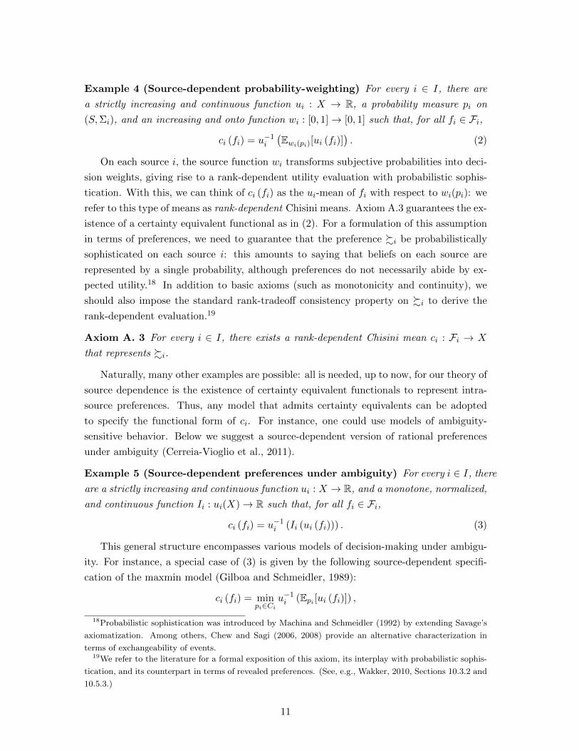
Example 4 (Source-dependent probability-weighting) For every i ∈ I, there are

a strictly increasing and continuous function ui : X → R, a probability measure pi on

(S,Σi), and an increasing and onto function wi : [0, 1]→ [0, 1] such that, for all fi ∈ Fi,

ci (fi) = u−1i

(Ewi(pi)[ui (fi)]

). (2)

On each source i, the source function wi transforms subjective probabilities into deci-

sion weights, giving rise to a rank-dependent utility evaluation with probabilistic sophis-

tication. With this, we can think of ci (fi) as the ui-mean of fi with respect to wi(pi): we

refer to this type of means as rank-dependent Chisini means. Axiom A.3 guarantees the ex-

istence of a certainty equivalent functional as in (2). For a formulation of this assumption

in terms of preferences, we need to guarantee that the preference %i be probabilistically

sophisticated on each source i: this amounts to saying that beliefs on each source are

represented by a single probability, although preferences do not necessarily abide by ex-

pected utility.18 In addition to basic axioms (such as monotonicity and continuity), we

should also impose the standard rank-tradeoff consistency property on %i to derive the

rank-dependent evaluation.19

Axiom A. 3 For every i ∈ I, there exists a rank-dependent Chisini mean ci : Fi → X

that represents %i.

Naturally, many other examples are possible: all is needed, up to now, for our theory of

source dependence is the existence of certainty equivalent functionals to represent intra-

source preferences. Thus, any model that admits certainty equivalents can be adopted

to specify the functional form of ci. For instance, one could use models of ambiguity-

sensitive behavior. Below we suggest a source-dependent version of rational preferences

under ambiguity (Cerreia-Vioglio et al., 2011).

Example 5 (Source-dependent preferences under ambiguity) For every i ∈ I, there

are a strictly increasing and continuous function ui : X → R, and a monotone, normalized,

and continuous function Ii : ui(X)→ R such that, for all fi ∈ Fi,

ci (fi) = u−1i (Ii (ui (fi))) . (3)

This general structure encompasses various models of decision-making under ambigu-

ity. For instance, a special case of (3) is given by the following source-dependent specifi-

cation of the maxmin model (Gilboa and Schmeidler, 1989):

ci (fi) = minpi∈Ci

u−1i (Epi [ui (fi)]) ,

18Probabilistic sophistication was introduced by Machina and Schmeidler (1992) by extending Savage’s

axiomatization. Among others, Chew and Sagi (2006, 2008) provide an alternative characterization in

terms of exchangeability of events.19We refer to the literature for a formal exposition of this axiom, its interplay with probabilistic sophis-

tication, and its counterpart in terms of revealed preferences. (See, e.g., Wakker, 2010, Sections 10.3.2 and

10.5.3.)

11

where Ci is a set of probabilities that reflects the perception of ambiguity on source i.20

We could also study source dependence in non-expected utility models that do not

involve ambiguity. For instance, if we replace the utility ui in Example 3 with a compact

set of utilities Ui, we obtain the following source-dependent specification of the cautious

expected utility model (Cerreia-Vioglio, Dillenberger, and Ortoleva, 2015), characterized

by heterogeneity of the utility sets across sources:

ci (fi) = minui∈Ui

u−1i (Epi [ui (fi)]) .

Note that an agent might be fully confident in a single utility function for a specific source,

thereby behaving as a standard expected utility maximizer over that source.

3.2 Inter-source preferences

Before turning to the overall relation % on F , we focus on its restriction to the space

P := (fi, i) : fi ∈ Fi. This subsection provides a characterization of preferences between

prospect-source pairs in P. The next axiom is key in relating monetary outcomes generated

by distinct sources.

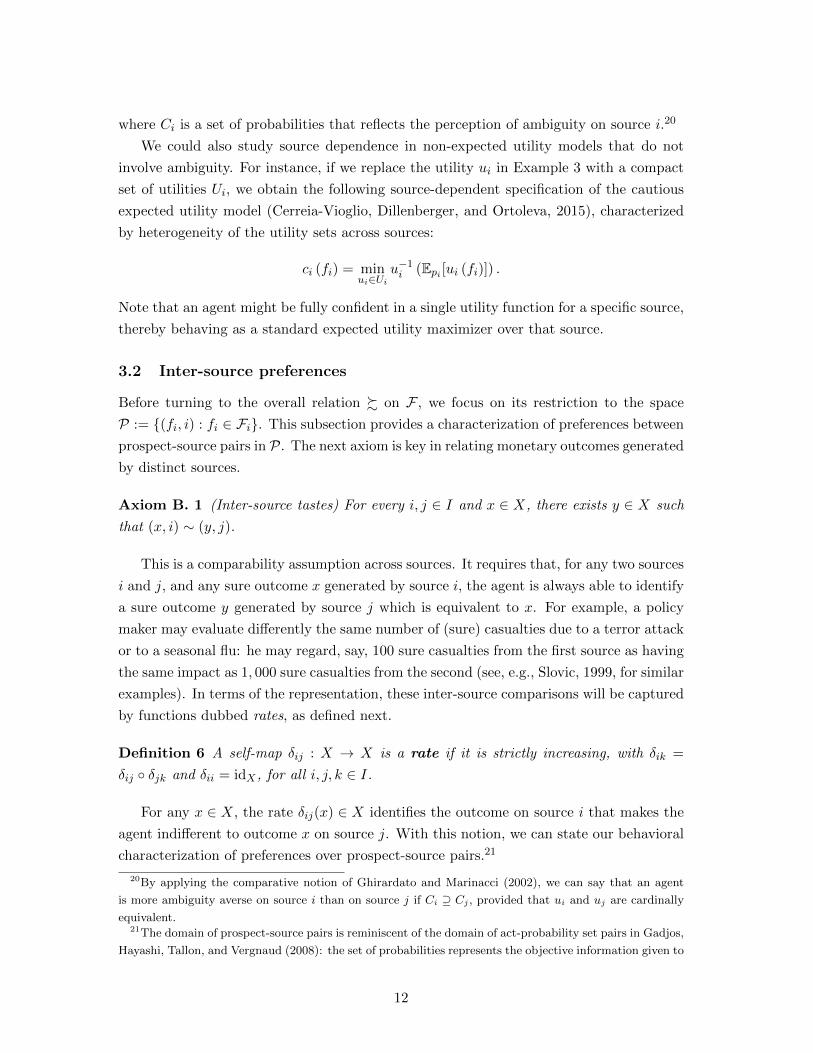
Axiom B. 1 (Inter-source tastes) For every i, j ∈ I and x ∈ X, there exists y ∈ X such

that (x, i) ∼ (y, j).

This is a comparability assumption across sources. It requires that, for any two sources

i and j, and any sure outcome x generated by source i, the agent is always able to identify

a sure outcome y generated by source j which is equivalent to x. For example, a policy

maker may evaluate differently the same number of (sure) casualties due to a terror attack

or to a seasonal flu: he may regard, say, 100 sure casualties from the first source as having

the same impact as 1, 000 sure casualties from the second (see, e.g., Slovic, 1999, for similar

examples). In terms of the representation, these inter-source comparisons will be captured

by functions dubbed rates, as defined next.

Definition 6 A self-map δij : X → X is a rate if it is strictly increasing, with δik =

δij δjk and δii = idX , for all i, j, k ∈ I.

For any x ∈ X, the rate δij(x) ∈ X identifies the outcome on source i that makes the

agent indifferent to outcome x on source j. With this notion, we can state our behavioral

characterization of preferences over prospect-source pairs.21

20By applying the comparative notion of Ghirardato and Marinacci (2002), we can say that an agent

is more ambiguity averse on source i than on source j if Ci ⊇ Cj , provided that ui and uj are cardinally

equivalent.21The domain of prospect-source pairs is reminiscent of the domain of act-probability set pairs in Gadjos,

Hayashi, Tallon, and Vergnaud (2008): the set of probabilities represents the objective information given to

12

Proposition 7 Let % be a binary relation on P. The following conditions are equivalent:

(i) % is a weak order that satisfies Axioms A.1 and B.1;

(ii) there exist

(a) a family (ci)i∈I of certainty equivalents for (%i)i∈I ,

(b) a family (δij)i,j∈I of rates,

such that, for all i, j ∈ I, fi ∈ Fi and gj ∈ Fj,

(fi, i) % (gj , j) ⇐⇒ ci (fi) ≥ δij (cj (gj)) . (4)

The elements of (ci)i∈I and (δij)i,j∈I are unique.

Representation (4) suggests a two-step procedure to compare prospect-source pairs.

First, the pairs (fi, i) and (gj , j) are independently evaluated by computing their certainty

equivalents, ci (fi) and cj (gj), respectively. For every source i, the function ci can be

viewed as a unit of account for that source. Second, the certainty-equivalent evaluations

are converted into the unit of account of one source. Such conversion is carried out by the

function δij which reflects the rate of substitution of outcomes between sources i and j.

In particular, representation (4) guarantees that, for any x, y ∈ X and i, j ∈ I,

(x, i) ∼ (y, j) ⇐⇒ x = δij(y) ⇐⇒ y = δji(x).

Thus, δij measures the value of a sure outcome on source j in terms of an equivalent out-

come on source i. The content of Proposition 7 lies in recognizing that source preferences

build on a distinction between intra-source uncertainty attitudes and inter-source tastes.

Diagrammatically:

Source Preferencesi = inter-source tastes︸ ︷︷ ︸δij

intra-source attitudes︸ ︷︷ ︸cj

The notion of inter-source tastes—the first component in the diagram—is the core novelty.

Different sources affect the desirability of outcomes, so that an agent may prefer receiving

(the sure) outcome x on source i rather than the same outcome on another source j.

Representation (4) states that inter-source tastes are identified by (δij)i,j . The rate δij can

be thought of as the cost of transporting one unit of consumption from source j to source

i, thereby capturing the (relative) subjective price of source j. Intra-source uncertainty

an agent in evaluating an act and can be viewed as a specific instance of source. In their setup, the ranking

of act-probability set pairs is always direct, i.e., the rate of substitution between sources is, implicitly, 1.

Hence, there is no need to introduce certainty equivalents and to adopt our two-step procedure. Their

approach captures the Ellsberg paradox in a way consistent with our related discussion.

13

attitudes—the second component in the diagram—correspond to a localized notion of

preferences under uncertainty. They are characterized by standard axioms imposed on

each source and are identified by the certainty equivalents.

Source preferences are determined by the composition of both features; yet, there are

prominent cases where they are driven by only one of them. To illustrate, consider the

two-urn Ellsberg paradox: as will be shown next, source preferences are determined solely

by intra-source uncertainty attitudes. On the other hand, in certain deterministic contexts

source preferences are generated solely by inter-source tastes: for instance, the comparison

of human casualties generated by different hazards (e.g., earthquakes, epidemics, terror

attacks, nuclear accidents) may be evaluated in different ways by policy makers taking

prevention measures. In this case, rates can be interpreted as the relative prices of hazards.

In general, both forces are at work. We bring to the fore two classic examples. First,

agents discount consumption at future dates in different ways (inter-source tastes), but

they might be more or less affected by outcomes’ variability at different dates (intra-source

attitudes). Second, agents attach different values to the same monetary payoff in different

markets (inter-source tastes) and, at the same time, they exhibit different (intra-source)

uncertainty attitudes on each market, as discussed in Section 6.

Two notable special cases easily follow from representation (4). We start by charac-

terizing the case of source-dependent expected utility, as seen in Example 3.

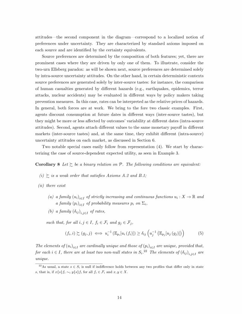
Corollary 8 Let % be a binary relation on P. The following conditions are equivalent:

(i) % is a weak order that satisfies Axioms A.2 and B.1;

(ii) there exist

(a) a family (ui)i∈I of strictly increasing and continuous functions ui : X → R and

a family (pi)i∈I of probability measures pi on Σi,

(b) a family (δij)i,j∈I of rates,

such that, for all i, j ∈ I, fi ∈ Fi and gj ∈ Fj,

(fi, i) % (gj , j) ⇐⇒ u−1i (Epi [ui (fi)]) ≥ δij

(u−1j

(Epj [uj (gj)]

))(5)

The elements of (ui)i∈I are cardinally unique and those of (pi)i∈I are unique, provided that,

for each i ∈ I, there are at least two non-null states in Si.22 The elements of (δij)i,j∈I are

unique.

22As usual, a state s ∈ Si is null if indifference holds between any two profiles that differ only in state

s, that is, if xsfi ∼i ysfi for all fi ∈ Fi and x, y ∈ X.

14

Next corollary extends the popular criterion of probabilistically sophisticated rank-

dependent utility to allow for source dependence, as described in Example 4.23

Corollary 9 Let % be a binary relation on P. The following conditions are equivalent:

(i) % is a weak order that satisfies Axioms A.3 and B.1;

(ii) there exist

(a) a family (ui)i∈I of strictly increasing and continuous functions ui : X → R, a

family (pi)i∈I of probability measures pi on Σi, and a family (wi)i∈I of increasing

and onto functions wi : [0, 1]→ [0, 1],

(d) a family (δij)i,j∈I of rates,

such that, for all i, j ∈ I, fi ∈ Fi and gj ∈ Fj,

(fi, i) % (gj , j) ⇐⇒ u−1i

(Ewi(pi)[ui (fi)]

)≥ δij

(u−1j

(Ewj(pj)[uj (gj)]

)). (6)

The elements of (ui)i∈I are cardinally unique and those of (pi)i∈I are unique, provided

that, for each i ∈ I, there are at least two non-null states in Si. The elements of (wi)i∈Iand (δij)i,j∈I are unique.

Corollaries 8 and 9 generalize the two main strands of the literature (respectively, the

utility approach and the probability-weighting approach) to situations where the compar-

ison between source-dependent prospects is not direct and it requires the application of a

conversion rate.

3.2.1 The expected utility case

An interesting special case occurs when the sure outcome x is on source j equivalent to

itself on source i.

Axiom B. 2 (Pecunia non olet) For every i, j ∈ I and x ∈ X, (x, i) ∼ (x, j).

This axiom requires that, when deterministic outcomes are concerned, the agent does

not discriminate between the sources generating them. Any difference in the evaluations of

uncertain prospects must be due solely to the agent holding different uncertainty attitudes

toward different sources. That is, the only perceived difference between sources is the

quality of the information about the stochastic nature of the states of the world.

When monetary payoffs are involved, the fact that deterministic outcomes are unaf-

fected by the stochastic nature of the underlying source rules out any consideration about

23Note that one can derive other probabilistically sophisticated non-expected utility specifications by

imposing suitable axioms on each intra-source preference %i.

15

the agent’s competence, thus making this assumption particularly transparent. Its behav-

ioral content can be summarized by the time-honored claim of Vespasian that pecunia non

olet — money has no smell. For instance, the value of a monetary outcome is the same on

both Ellsberg urns. That said, one can think of situations in which this assumption would

be too restrictive: it is likely that a person would not be indifferent between receiving the

same monetary profit from legal versus illegal entrepreneurial activities.24

Replacing Axiom B.1 with Axiom B.2 in Proposition 7 is immediately seen to corre-

spond to δij = idX for all i, j ∈ I. Then, representation (4) reduces to

(fi, i) % (gj , j) ⇐⇒ ci (fi) ≥ cj (gj) . (7)

In view of the importance of expected utility, we present a special case of Proposition 7

where certainty equivalents can be directly compared—without the mediation of the rates

δij as in Corollary 8—and, at the same time, they conform to subjective expected utility.

Proposition 10 Let % be a binary relation on P. The following conditions are equivalent:

(i) % is a weak order that satisfies Axioms A.2 and B.2;

(ii) there exist a family (ui)i∈I of strictly increasing and continuous functions ui : X →R, and a family (pi)i∈I of probability measures pi on Σi, such that, for all i, j ∈ I,

fi ∈ Fi and gj ∈ Fj,

(fi, i) % (gj , j) ⇐⇒ u−1i (Epi [ui (fi)]) ≥ u−1

j

(Epj [uj (gj)]

). (8)

The elements of (ui)i∈I are cardinally unique and those of (pi)i∈I are unique, provided

that, for each i ∈ I, there are at least two non-null states in Si.

In representation (8), source dependence manifests itself only in the potentially dif-

ferent uncertainty attitudes, whereas the value of a deterministic outcome is source inde-

pendent. This is an important special case of our model as it offers a formal treatment of

the utility approach in alternative to the more traditional probability-weighting approach.

We illustrate the differences between these two approaches by applying them to resolve

the classic two-urn Ellsberg paradox.

Two-urn Ellsberg experiment Denote by I = 1, 2 the set of urns and by Si =

Redi,Blacki the set of states for each i ∈ I. Urn 1 contains 50 red and 50 black balls,

while Urn 2 has unknown composition. Let fi (resp., gi) be the bet that pays $100 if the

ball drawn from urn i ∈ I is red (resp., black) and $0 otherwise. The typical pattern is

f1 ∼ g1 g2 ∼ f2. Most subjects are indifferent between betting on red or on black from

either urn; yet, they strictly prefer to bet on Urn 1 rather than on Urn 2.

24As mentioned earlier, Slovic (1999) contains various examples, mostly in the context of casualties.

16

Source preferences generate a ‘paradox’ because indifference between betting on red or

on black from either urn suggests that the two states are perceived as equally likely; but,

if subjects assign also the same utilities to the same consequences generated by different

sources, then the certainty equivalents of all the four bets must be the same. This is

clearly inconsistent with a preference for betting on the known urn.

The source-dependent utility criterion developed in Proposition 10 can rationalize the

observed pattern by maintaining the same equal probability of the states, while allowing

for utilities to depend on sources as follows:

c1 (f1) = u−11

[1

2u1 (100) +

1

2u1 (0)

]6= u−1

2

[1

2u2 (100) +

1

2u2 (0)

]= c2 (f2) ,

explaining the pattern if u1 is less concave than u2. Early discussions of this approach

appear in Fellner (1961), Roberts (1963), Smith (1969), and, more recently, in Chew

et al. (2008). On the other hand, the dominant approach in the literature follows the

seminal papers of Kahneman and Tversky (1979) and Schmeidler (1989) by focussing on

source-dependent probability distortions as follows:

c1 (f1) = u−1

[w1

(1

2

)u (100) + w1

(1

2

)u (0)

]6= u−1

[w2

(1

2

)u (100) + w2

(1

2

)u (0)

]= c2 (f2) ,

explaining the pattern if w1 > w2.

3.3 Preferences over prospect profiles

It remains to study the preferences % over the entire domain F of prospect profiles. We

posit the following basic axiom.

Axiom C. 1 The binary relation % on F is a weak order such that:

(i) (Monotonicity) if f ,g ∈ F and fi %i gi for all i ∈ I, then f % g;

(ii) (Strict Monotonicity) if both x and y in XI are constant and x > y, then x y;

(iii) (Archimedean Continuity) if x,y, z ∈ XI and x y z, then there exist α, β ∈(0, 1) such that

(1− α) x + αz y (1− β) x + βz.

Axiom C.1 can be viewed as the analogue of Axiom A.1 over the richer domain of

prospect profiles. Property (i) maintains that the agent should prefer a profile f to another

profile g whenever f consists of better source-dependent prospects than g, source-by-

source. Property (ii) is a form of strict monotonicity imposed on fully constant prospect

17

profiles. Property (iii) is a standard continuity property which, together with the other

assumptions in Axiom C.1, guarantees that, for any f ∈ F , the agent can find a fully

constant profile x which is indifferent to f .

4 Representation results

This section provides behavioral characterizations of source-dependent preferences over

prospect profiles—the domain of central interest of our theory. We start with a general

utility structure that captures the essential features of source-dependent preferences.

4.1 General representation result

The following terminology will be useful to state our results.

Definition 11 A monotone and continuous functional D : XI → X is

(i) an aggregator if it is normalized, that is, D(x1I) = x for all x ∈ X;

(ii) an aggregator at the numeraire i ∈ I if it is i-normalized, that is, D(x1i) = x

for all x ∈ X.

We are now ready to state our general representation result. It disentangles the two

behavioral features that may give rise to source dependence, namely intra-source attitudes

and inter-source tastes, within the rich domain of prospect profiles.

Theorem 12 Let % be a binary relation on F . The following conditions are equivalent:

(i) % satisfies Axioms A.1, B.1, and C.1;

(ii) there exist

(a) a family (ci)i∈I of certainty equivalents for (%i)i∈I ,

(b) a family (δij)i,j∈I of rates,

such that, for all i, j ∈ I, fi ∈ Fi, and gj ∈ Fj,

(fi, i) % (gj , j) ⇐⇒ ci (fi) ≥ δij (cj (gj)) ,

(c) an aggregator at the numeraire o ∈ I, Wo : XI → X, such that, for every

f = (fi)i∈I ,

Vo (f) = Wo (δo1 (c1 (f1)) , . . . , δon (cn (fn))) (9)

represents % on F .

18

According to representation (9), a prospect profile is first evaluated source-wise, with

each source i’s own unit of account given by ci. Each of these evaluations is then converted

into the unit of account of a posited numeraire source o by applying the conversion rates δoi.

Finally, this profile of evaluations is aggregated in a unique evaluation given by Wo which

preserves the normalization to source o. Thus, Wo is an aggregator of source-dependent

deterministic payoffs evaluated through the lens of the numeraire o.25

By Theorem 12, we can represent a binary relation % on F that satisfies Axioms

A.1, B.1, and C.1 by a triple ((ci)i∈I , (δij)i,j∈I ,Wo). We refer to such a triple as a

source-dependent representation of %. Our utility representation has standard uniqueness

properties, as shown next.

Proposition 13 Let % be a binary relation on F that satisfies the assumptions of Theo-

rem 12. Then, the following statements hold:

(i) for every o ∈ I, the source-dependent representation ((ci)i∈I , (δij)i,j∈I ,Wo) of % is

unique;

(ii) if o 6= o and ((ci)i∈I , (δij)i,j∈I ,Wo) and ((ci)i∈I , (δij)i,j∈I ,Wo) are two source-

dependent representations of %, then Wo = δoo (Wo).

Theorem 12 serves the purpose of providing a general framework and an axiomatic

foundation that captures the core features of source-dependent preferences. It encompasses

numerous special cases which vary in the functional specifications of the aggregator Wo and

the rates δij (as well as the forms of the certainty equivalents, as illustrated in Examples

3-5). For instance, one could think of non-additive aggregators (in the spirit of Choquet

expected utility (Schmeidler, 1989) or maxmin preferences (Gilboa and Schmeidler, 1989)

to introduce considerations of ambiguity in the process of evaluating sources. On the other

hand, Theorem 12 does not suggest an operational criterion to adopt in applied problems.

We next address this point by introducing important special cases.

4.2 Quasi-arithmetic aggregators

This section considers a structured specification of the aggregator Wo and focuses on

the well-known special case of quasi-arithmetic means. We will see that the class of

quasi-arithmetic aggregators is analytically tractable and accommodates classic utility

specifications used in applied economic settings.

For the rest of this section, we assume that X = R and impose few additional properties

on % restricted to the domain of constant prospect profiles. We begin with a standard

continuity assumption.

25In Appendix A.2, Theorem 20 provides an alternative utility representation according to which the

agent evaluates prospect profiles without committing to a specific numeraire.

19

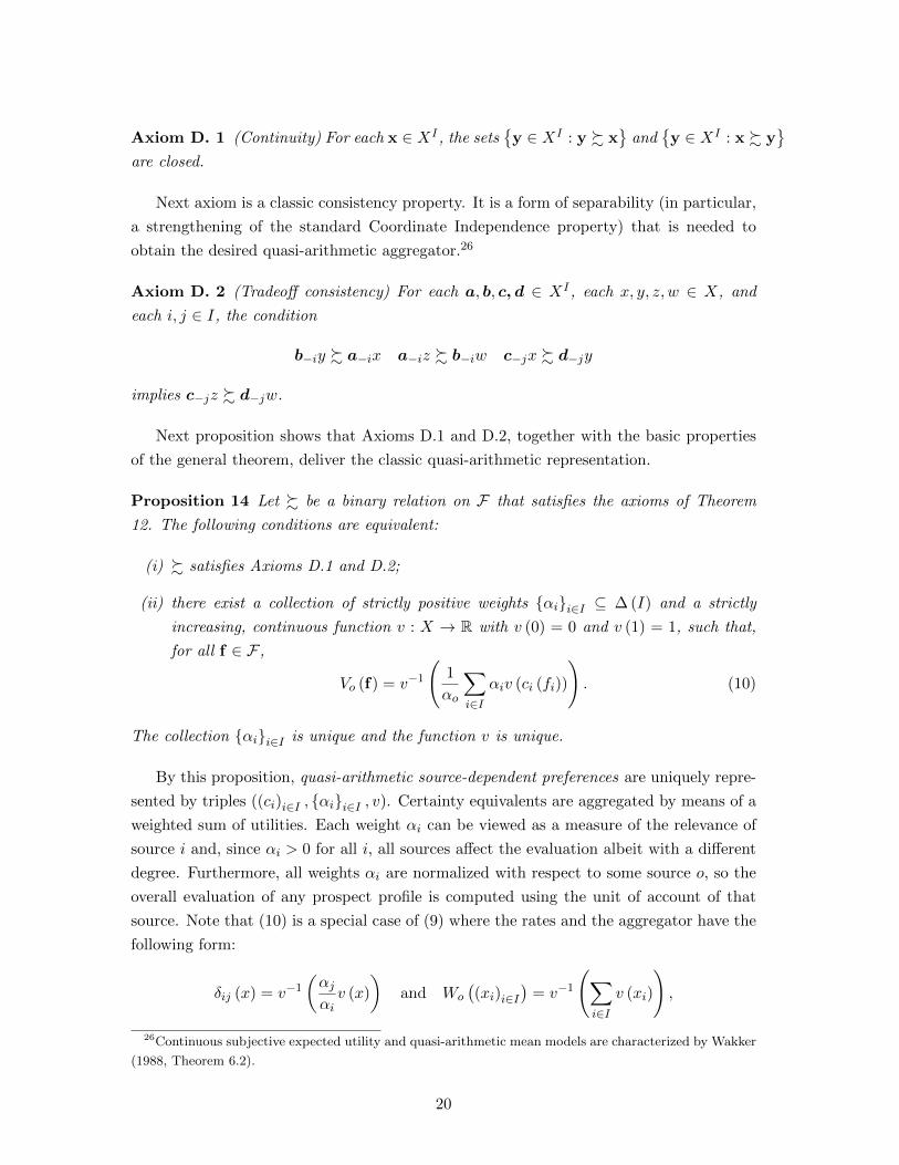
Axiom D. 1 (Continuity) For each x ∈ XI , the setsy ∈ XI : y % x

and

y ∈ XI : x % y

are closed.

Next axiom is a classic consistency property. It is a form of separability (in particular,

a strengthening of the standard Coordinate Independence property) that is needed to

obtain the desired quasi-arithmetic aggregator.26

Axiom D. 2 (Tradeoff consistency) For each a, b, c, d ∈ XI , each x, y, z, w ∈ X, and

each i, j ∈ I, the condition

b−iy % a−ix a−iz % b−iw c−jx % d−jy

implies c−jz % d−jw.

Next proposition shows that Axioms D.1 and D.2, together with the basic properties

of the general theorem, deliver the classic quasi-arithmetic representation.

Proposition 14 Let % be a binary relation on F that satisfies the axioms of Theorem

12. The following conditions are equivalent:

(i) % satisfies Axioms D.1 and D.2;

(ii) there exist a collection of strictly positive weights αii∈I ⊆ ∆ (I) and a strictly

increasing, continuous function v : X → R with v (0) = 0 and v (1) = 1, such that,

for all f ∈ F ,

Vo (f) = v−1

(1

αo

∑i∈I

αiv (ci (fi))

). (10)

The collection αii∈I is unique and the function v is unique.

By this proposition, quasi-arithmetic source-dependent preferences are uniquely repre-

sented by triples ((ci)i∈I , αii∈I , v). Certainty equivalents are aggregated by means of a

weighted sum of utilities. Each weight αi can be viewed as a measure of the relevance of

source i and, since αi > 0 for all i, all sources affect the evaluation albeit with a different

degree. Furthermore, all weights αi are normalized with respect to some source o, so the

overall evaluation of any prospect profile is computed using the unit of account of that

source. Note that (10) is a special case of (9) where the rates and the aggregator have the

following form:

δij (x) = v−1

(αjαiv (x)

)and Wo

((xi)i∈I

)= v−1

(∑i∈I

v (xi)

),

26Continuous subjective expected utility and quasi-arithmetic mean models are characterized by Wakker

(1988, Theorem 6.2).

20

for all x ∈ X and all (xi)i∈I ∈ XI . Finally, the form of the utility v captures a preference

for smoothing across sources, as shown by our comparative statics analysis later on.

Before moving on, let us recall that the class of quasi-arithmetic means is closely related

to classic utility models in economics. Indeed, representation (10) conforms essentially to

subjective expected utility if the certainty equivalent functionals are quasi-linear as in

Example 3, and the utilities ui’s in that example are such that ui = v for all i ∈ I.

Standard temporal and allocation settings can be cast as special cases of the quasi-

arithmetic source-dependent model. Importantly, we will next see that, in these applied

settings, the numeraire earns precise economic content.

4.3 Temporal sources

By viewing consumption dates as temporal sources, this section studies intertemporal

preferences within our framework of source dependence. A key advantage of taking a

source perspective is to allow for time-dependent uncertainty attitudes. The same source

of risk (e.g., financial risk) evaluated at different ages or time horizons may affect agents

in different ways; this may naturally generate different risk attitudes in a way consistent

with the empirical evidence, as argued in the Introduction.

Let I = 0, 1, . . . , T be interpreted as a set of dates. A prospect profile f = (f0, . . . , fT )

is a temporal stream of consumption where ft denotes the bundle consumed at time t ∈ I.

We impose the following stationarity assumption.

Axiom D. 3 (Stationarity) If s, t ∈ I\ T and x, y ∈ X, then

(x, s) ∼ (y, t) =⇒ (x, s+ 1) ∼ (y, t+ 1) .

The above axiom preserves the well-known behavioral content of stationarity: the

indifference between two time-dependent consequences hinges on the dates s and t, whereas

it is not affected by postponing consumption of both consequences by the same amount of

time. We next show that familiar exponential discounting utility models can be recovered

as special cases of our quasi-arithmetic source-dependent representation.

Proposition 15 Let % be a binary relation on F that satisfies the axioms of Theorem

12. The following conditions are equivalent:

(i) % satisfies Axioms D.1, D.2, and D.3;

(ii) there exist a scalar β > 0 and a strictly increasing, continuous function v : X → Rwith v (0) = 0 and v (1) = 1, such that, for all f ∈ F ,

V0 (f) = v−1

(T∑t=0

βtv (ct (ft))

). (11)

21

The scalar β and the function v are unique.

According to (11), the agent evaluates f by first computing the time-t certainty equiva-

lent of each component ft. Time-t certainty equivalent captures the risk attitude exhibited

over time-t horizon. The overall evaluation is given by the discounted sum of utilities of

(time-dependent) certainty equivalents. From our source perspective, the discount factor

is the price of time: in particular, it can be viewed as the cost of transporting one unit of

consumption between different dates. Moreover, the choice of the numeraire o is simple

since, as usual in applied temporal contexts, the value of a stream is discounted at time

0. Indeed, (11) is a special case of (9) where

δij (x) = v−1(βj−iv (x)

)and W0

((xi)i∈I

)= v−1

(∑i∈I

v (xi)

),

for all x ∈ X and all (xi)i∈I ∈ XI . The aggregator W0 (x) can be thought of as the value

of a perpetuity that is exactly as good as x itself.

Note that representation (11) reduces to standard discounted utility over constant

prospect profiles. Furthermore, one can specify the certainty equivalents as in Example

3 and set ct (ft) = u−1t

(∫S ut (ft) dpt

), where ut is a utility function on X and pt is a

probability measure on S for all t = 0, ..., T . In the extreme case in which ut = v for all

t = 0, ..., T , we recover the standard discounted expected utility criterion with no source

effects and constant risk aversion:

V0 (f) = v−1

(T∑t=0

βt∫Sv (ft) dpt

).

We conclude this section by briefly relating our model to some existing works on

horizon-dependent risk attitudes. If we consider a set I = 0, 1 of only two dates,

representation (11) can be rewritten as

v−1 ((1− β) v (c0 (f0)) + βv (c1 (f1))) ,

which corresponds to the case studied in Andries et al. (2018) who distinguish between

two levels of risk aversion toward immediate and delayed uncertainty, respectively. By

allowing for levels of risk aversion that are decreasing with the time horizon, they generate

predictions consistent with the empirical evidence on the term structure of equity returns.

5 Comparative attitudes

The additional structure of the quasi-arithmetic model allows us to develop a comparative

statics analysis of the effects of inter-source smoothing on choice behavior.

Consider an agent with quasi-arithmetic source-dependent preferences represented by

((ci)i∈I , αii∈I , v). We say that the agent has a preference for source smoothing if, for

22

any x = (xi)i∈I ∈ XI , he prefers the profile that yields the quasi-arithmetic v-mean of

x on all sources to x itself. That is, if we denote by z = v−1(

1αo

∑i∈I αiv (xi)

)∈ X

such a mean, we must have (z, z, . . . , z) % x.27 This definition is reminiscent of the

classic notion of risk aversion with an important caveat: our notion of source smoothing

applies to prospect profiles that do not involve any risk as they are constant within each

source. Risk aversion, instead, pertains to intra-source attitudes and is captured by the

source-dependent certainty equivalents. The latter do not play any role here.

Consider two agents with preferences given by %1 and %2. We posit that %1 has a

higher preference for source smoothing than %2 if and only if, for all x ∈ XI and z ∈ X,

x %1 (z, z, ..., z) =⇒ x %2 (z, z, ..., z) .

In words, %1 has a higher preference for source smoothing than %2 if, whenever %1 prefers

a non-constant outcome profile across sources to a constant one, then the same is true for

%2. Next result provides a behavioral characterization and shows that the comparative

attitudes toward source smoothing are controlled by the function v.

Proposition 16 Let %1 and %2 be two quasi-arithmetic source-dependent preferences rep-

resented by (α1i

i∈I , v1) and (

α2i

i∈I , v2), respectively. The following conditions are

equivalent:

(i) %1 has a higher preference for source smoothing than %2;

(ii)α1i

i∈I =

α2i

i∈I and v1 = ψ v2 for some concave, strictly increasing, and con-

tinuous transformation ψ : v2(X)→ v1(X).

This proposition states that higher preferences for source smoothing are characterized

by more concave utility functions v. As anticipated earlier, this result resembles the

standard comparative characterization of risk aversion.28 In turn, our result captures a

form of aversion to the variance of outcomes across sources.

When I = 0, 1, . . . , T is interpreted as a set of dates, the notion of higher preference

for source smoothing corresponds to the familiar notion of higher preference for intertem-

poral smoothing. As an immediate corollary of the above proposition, we conclude that in

the intertemporal setting of Proposition 15, %1 has a higher preference for intertemporal

smoothing than %2 if and only if β1 = β2 and v1 is more concave than v2.

6 A portfolio allocation problem

This section adopts our quasi-arithmetic model to introduce source dependence into a

simple financial allocation problem. We examine the implications on the optimal portfolio

allocation and the relationship with some well-known empirical puzzles.

27Here (z, z, . . . , z) ∈ XI is the constant profile that yields outcome z on all sources.28See, e.g., Wakker (1989, Definition VII.6.4).

23

6.1 Market and subjective prices

Consider an agent who faces the following investment problem: there are two assets (f1, f2)

in two different markets, say Eurozone and US, with prices (p1, p2) ∈ R2++ and he has to

decide how to allocate his wealth w = (w1, w2) ∈ R2++ across these two assets (prices

and wealth are denominated in the local currencies). Each asset is modeled as a random

variable fi : Si → [0,∞) that pays in the local currency and depends on a local source of

uncertainty. In view of our theory, we can set I = 1, 2, where source 1 (resp., source 2)

identifies the Eurozone market (resp., the US market).

The agent can buy ξi ≥ 0 units of asset i (short-sales are not possible), forming a

portfolio ξ = (ξ1, ξ2). He can move money from one market to the other, once converted

in the same currency through a market exchange rate. We denote by ρij the market

(nominal) exchange rate from currency j to currency i; so, ρ12 says how many euros the

market trades for 1 dollar. The budget constraint is then:

ξ1, ξ2 ≥ 0, ξ1p1 + ξ2ρ12p2 ≤ w1 + ρ12w2. (12)

Here, the real exchange rate is e12 = ρ12p2/p1, which states how many units of the

Eurozone asset the market trades for 1 unit of the US asset.

Each portfolio ξ determines the random profile (ξ1f1, ξ2f2). The agent evaluates each

payoff ξifi separately, according to the source-dependent criterion

ci (ξifi) = u−1i

(∫Si

ui (ξifi) dqi

), (13)

where ui is a strictly increasing, strictly concave, and continuous function, and qi is a

probability measure on Si. As seen next, we posit that each ui has a CRRA form so that

ci (ξifi) = ξici (fi).29 Using the quasi-arithmetic specification of Proposition 14, the agent

aggregates the evaluations in (13) according to the function W : R2+ → R given by

W (ξ1, ξ2) = v−1 (α1v (ξ1c1 (f1)) + α2v (ξ2c2 (f2))) ,

where α1, α2 ∈ (0, 1) and α1 + α2 = 1. Assume that, for each i, there exists γi ∈ (0, 1)

such that

ui(x) =x1−γi

1− γifor all x ≥ 0,

and there exists k ∈ (0, 1) such that

v(x) =x1−k

1− kfor all x ≥ 0.

Let δ21 = δ21 (1) stand for how many dollars are subjectively equivalent to a payoff of 1

euro. Thus, δij is a subjective price and we refer to it as the (nominal) subjective exchange

29To make the problem nontrivial, we also assume that c1 (f1) , c2 (f2) > 0.

24

rate. By quantifying the subjective value of one currency in terms of the other, δij is

interpreted as a measure of familiarity toward one market relative to another (which in

turn determines how outcomes are evaluated in the two markets). We next show that

subjective exchange rates play a key role in determining the optimal portfolio allocation.

Proposition 17 The unique optimal portfolio ξ = (ξ1, ξ2), provided it is an interior so-

lution, is such that

p1ξ1

ρ12p2ξ2

=

(e12

δ21c1 (f1)

c2 (f2)

) 1−kk

, (14)

where δ21 =(α1α2

) 11−k

. Moreover, ∂W∂ξ2

(ξ)/∂W∂ξ1

(ξ) = ρ12p2/p1 = e12.

The left-hand side of (14) is the ratio of the optimal investments in each market,

expressed in euros via the nominal exchange rate. The right-hand side is a function of

the product, also expressed in euros, of the objective e12 and subjective δ21c1 (f1) /c2 (f2)

terms of trade between the two assets. In particular, δ21c1 (f1) /c2 (f2) is the ratio of the

subjective values of each euro invested in each market.

The relation between subjective and market exchange rates in (14) reminds the classic

relation between subjective discount rates and market interest rates that characterizes

Euler equations in intertemporal consumption problems. Indeed, (14) is a spatial counter-

part of the classic temporal relation. Across time or space, optimality imposes a tradeoff

between market prices and subjective traits.

6.2 Comparative analysis and home bias

The last proposition derives the optimal portfolio allocation of an agent with quasi-

arithmetic source-dependent preferences and formalizes the way subjective exchange rates

affect financial decisions. In the special case δ21 = 1, the agent perceives a payoff of 1

euro as subjectively equivalent to a payoff of 1 dollar and, therefore, he is equally familiar

about the value of euros versus dollars. This means that he may still exhibit source-

dependent uncertainty attitudes, reflected in the certainty equivalents c1 and c2; however,

once uncertainty is factored out, he finds monetary outcomes generated by either source

as perfectly comparable, analogously to what we have seen in the two-urn Ellsberg exper-

iment.30 Condition (14) then reduces to

p1ξ1

ρ12p2ξ2

=

(e12

c1 (f1)

c2 (f2)

) 1−kk

, (15)

and the ratio of the optimal investments depends only on the market exchange rate e12.

On the other side, if δ21 > 1, then a payoff of 1 euro is worth more for the agent than

a payoff of 1 dollar. By comparing (14) to (15), we conclude that, ceteris paribus, the

30Note that δ21 = 1 does not necessarily imply that the market (nominal) exchange rate ρ21 is 1, as well.

25

more δ21 exceeds 1, the more the agent will invest in asset 1. This observation suggests an

explanation of the evidence on home bias and under-diversification in terms of familiarity.

Taking the perspective of a Eurozone investor, the higher is the degree of familiarity for

the Eurozone in comparison to the US zone (i.e., the higher δ21 is), the higher will be the

inclination to invest in the Eurozone asset.

The role of δ21 is analogous to the one played by a subjective discount factor β in

temporal settings. The lower the subjective discount factor is, the higher the (market)

real interest rate must be to compensate for the investor’s impatience. Here, the higher

the subjective exchange rate δ21 is, the lower the (real) market exchange rate e12 needs to

be to compensate for the familiarity bias toward the Eurozone. In a vein akin to the classic

temporal Euler equation, these opposing forces can be seen in action in condition (14).

We conclude with a comparative analysis of how each parameter affects the optimal

portfolio allocation. First, note that the higher the coefficient k is, the more concave the

function v is. By Proposition 16, it follows that k is an index of the agent’s preference for

source smoothing (i.e., preference for constant profiles across sources). Now, denote by

ξi = ξiw1+ρ12w2

the optimal share of asset i which measures the fraction of wealth invested

in asset i.

Proposition 18 Let ξ = (ξ1, ξ2) be the unique optimal portfolio satisfying condition (14)

of Proposition 17 and ξ = (ξ1, ξ2) be the resulting vector of asset shares. Then,

∂ξi∂αi

> 0,∂ξi∂γi

< 0, and∂ξi∂pi

< 0 for i = 1, 2.

A higher weight αi reflects a stronger familiarity bias for source i and induces a higher

share of asset i. Moreover, a higher coefficient of uncertainty aversion γi within source i

yields a lower share of asset i. Finally, a higher price pi yields a lower share of asset i.

7 Concluding remarks

This paper develops a unifying framework that incorporates existing approaches to study

choice problems in the presence of multiple sources. We show that source preference origi-

nates from two behavioral features represented by source-dependent certainty equivalents

and subjective prices. The notion of subjective price is the key novelty. It has a precise

economic content in terms of subjective rates of substitution between sources. Their role

is to enable comparisons of prospects across different sources. We illustrate the distinction

between these two features in the settings of intertemporal and allocation choices, as well

as comparisons of hazards. We close with two remarks on the limitation of our framework

and indicate possible directions for future research.

26

Source interdependence Our setup does not explicitly account for source-dependent

prospects that depend simultaneously on multiple sources. This is compatible with many

contexts (notably with intertemporal settings), but it can be restrictive on occasion. While

a systematic analysis of this issue is beyond the scope of this paper, our setup can easily

be extended to accommodate some forms of multiple dependence. To illustrate, consider

the allocation problem of Section 6 where each asset is a source-dependent prospect that

depends only on one source, the Eurozone market (source 1) or the US market (source

2). Suppose that an additional source, say the Asian market (source 3), influences the

performance of both assets. Indeed, a financial crisis in Asia is likely to affect both the

Eurozone and the US. This issue can be addressed within our setup by viewing it as a

form of interdependence between sources. Let Si = Si × S3 stand for the set of effective

contingencies for market i = 1, 2. That is, Si describes the relevant uncertainty on market

i by taking into account all possible combinations of contingencies featured by the local

source i and the Asian source. Asset i is then defined as fi : Si → [0,∞) for i = 1, 2. As

before, fi pays in the local currency, but now it depends on the interactions between the

local source (Eurozone or US) and the external source (Asia) that, together, determine

the payoff structure of the asset. By affecting the underlying mechanism of uncertainty,

this interdependence may alter the source-dependent uncertainty attitudes: the certainty

equivalent in (13) is now computed with respect to a probability measure defined on the

extended set of contingencies Si. The definition of the remaining parameters is formally

unchanged. In particular, all exchange rates are still defined between euros and dollars.

Any influence of the Asian source on the Eurozone and the US is captured by the respective

certainty equivalents and assessed using one of the two currencies. Hence, the analysis of

the last section remains valid within this extended setup. A natural direction for future

research is the study of more complicated forms of interdependence and their potential

impact on the familiarity perception of markets as captured by subjective prices.

Source elicitation Our work does not address the question of how sources could be

elicited from choices—they are exogenously given. This is certainly a limitation of our

approach. In more specific settings, other works in the literature, notably Chew and Sagi

(2008), Abdellaoui, Baillon, Placido, and Wakker (2011), and Gul and Pesendorfer (2015)

identify sources subjectively, through collections of events that satisfy certain properties.

Nevertheless, we should remark that, in many decision problems, sources are natu-

rally defined by the framework itself. Moreover, agents can often choose which source to

act upon in a way consistent with our representation of preferences over prospect-source

pairs. We study several contexts of this sort: the two urns in the Ellsberg paradox, dates

in temporal settings, and locations in portfolio allocation settings. We leave the more

decision-theoretic question of elicitation as a direction for future research.

27

A Proofs and related analysis

A.1 Proofs of the results of Section 3

Proof of Lemma 2. It follows directly from Lemma 24 (in Online Appendix) by letting

Ω = S and F = Fi in that lemma.

Proof of Proposition 7. (i) implies (ii). Since % satisfies Axiom A.1, it follows from

Lemma 2 that there exists a family (ci)i∈I of certainty equivalents for (%i)i∈I .

Fix i, j ∈ I. By Axiom B.1, for every x ∈ X, there exists y ∈ X such that (x, i) ∼ (y, j).

Note that the number y is unique. In fact, by transitivity of % on P, if y ∈ X were

such that (x, i) ∼ (y, j), then (y, j) ∼ (y, j). That is, (y, j) ∼j (y, j), yielding that

y = cj (y) = cj (y) = y. By the same reasoning, note that if i = j, then y = x. Thus, we

can define a function δji : X → X as

δji (x) = y where y is such that (x, i) ∼ (y, j). (16)

Note that if i = j, then δii = idX . Since i, j ∈ I were arbitrarily chosen, we have that

δji : X → X, defined as in (16), is a well-defined function. Next, we show that, for all

i, j ∈ I, δji is a rate and, hence, it satisfies the properties described in Definition 6.

• If x > z, then (x, i) (z, i) by Axiom A.1(i) and the definition of %i. By con-

tradiction, assume that δji (x) ≤ δji (z). Then, by Axiom A.1(i), it follows that

(δji (z) , j) % (δji (x) , j). By construction, we also have that (z, i) ∼ (δji (z) , j) %

(δji (x) , j) ∼ (x, i), yielding, by transitivity, that (z, i) % (x, i), a contradiction. This

proves that δji is strictly increasing.

• By construction, for every y ∈ X, (y, j) ∼ (δij (y) , i), that is, y = δji (δij (y)). Thus,

δji is onto (and δij = δ−1ji ).

• By construction, for every x ∈ X and k ∈ I, (x, i) ∼ (δji (x) , j) and (δji (x) , j) ∼(δkj (δji (x)) , k). By transitivity, this implies that (x, i) ∼ (δkj (δji (x)) , k), that is,

δkj (δji (x)) = δki (x). Thus, δki = δkj δji.

Now, let i, j ∈ I, fi ∈ Fi, and gj ∈ Fj . By the previous part of the proof, we have

(fi, i) ∼ (ci (fi) , i) , (gj , j) ∼ (cj (gj) , j) , and (cj (gj) , j) ∼ (δij (cj (gj)) , i).

By transitivity of % on P and Lemma 2, we obtain that

(fi, i) % (gj , j) ⇐⇒ (ci (fi) , i) % (cj (gj) , j)

⇐⇒ (ci (fi) , i) % (δij (cj (gj)) , i) ⇐⇒ ci (fi) ≥ δij (cj (gj)) ,

(ii) implies (i). Let i ∈ I and fi, gi ∈ Fi. Then,

(fi, i) % (gi, i) ⇐⇒ ci (fi) ≥ δii (ci (gi)) ⇐⇒ ci (fi) ≥ ci (gi) .

28

Since i was arbitrarily chosen, it follows that % on P is a complete binary relation. Next,

if (fi, i) % (gj , j) and (gj j) % (hk, k), then representation (4) implies that

ci (fi) ≥ δij (cj (gj)) and cj (gj) ≥ δjk (ck (hk)) .

Since δij is increasing and onto and δki = δkj δji, we have

ci (fi) ≥ δij (cj (gj)) ≥ δij (δjk (ck (hk))) = δik (ck (hk)) ,

that is, (fi, i) % (hk, k), proving that % on P is transitive, too.

Since ci is a certainty equivalent functional, we can apply Lemma 2 and directly con-

clude that %i on Fi satisfies Axiom A.1.

Finally, for every i, j ∈ I and x ∈ X, let y = δji (x). Then,

cj (y) = y = δji (x) = δji (ci (x)) ,

proving that (y, j) ∼ (x, i). Thus, Axiom B.1 is satisfied.

The uniqueness of (ci)i∈I follows from Lemma 2. Next, assume that (δji)j,i∈I is another

family of functions that, together with (ci)i∈I , represents % on P as in (4). Fix arbitrary

i, j ∈ I. It follows that, for all x ∈ X,

(x, i) ∼ (δji (x) , j) and (x, i) ∼ (δji (x) , j).

By transitivity of %, we have (δji (x) , j) ∼ (δji (x) , j) which, by using the representation,

implies δji (x) = δji (x). We conclude that δij = δij for all i, j ∈ I.

Proofs of Corollaries 8 and 9. (i) implies (ii). By Proposition 7, there exist a family

(ci)i∈I of certainty equivalents for (%i)i∈I , and a family (δij)i,j∈I of rates, such that, for

all i, j ∈ I, fi ∈ Fi and gj ∈ Fj , (fi, i) % (gj , j) iff ci (fi) ≥ δij (cj (gj)). Moreover, for

each i ∈ I, ci : Fi → X is unique. Thus, we can apply Axioms A.2 and A.3 which directly

yield representations (5) and (6), respectively.

It is immediate to verify that (ii) implies (i) for both corollaries. The uniqueness parts

follow from Proposition 7 and standard arguments (see, e.g., Wakker, 1989, Observation

IV.2.7, and Wakker, 2010, Observation 10.5.6, respectively).

Proof of Proposition 10. (i) implies (ii). By Axiom A.2, for every i ∈ I, there are

a strictly increasing and continuous function ui : X → R and a probability measure pi

on (S,Σi) such that ci : Fi → X represents %i where ci(fi) = u−1i

(∫S ui (fi) dpi

)for all

fi ∈ Fi. Fix arbitrary i, j ∈ I, fi ∈ Fi, and gj ∈ Fj and suppose that (fi, i) % (gj , j). By

Axiom A.2, we have (fi, i) ∼ (ci(fi), i) and (gj , j) ∼ (cj(gj), j). By Axiom B.2, (ci(fi), i) ∼(ci(fi), j). Then, transitivity implies (ci(fi), j) % (cj(gj), j), that is, ci(fi)1Sj %j cj(gj)1Sj .

Since cj represents %j , we conclude that ci(fi) ≥ cj(gj).

It is immediate to verify that (ii) implies (i). The uniqueness part follows from standard

arguments (see, e.g., Wakker, 1989, Observation IV.2.7).

29

A.2 Proofs of the results of Section 4

In the rest of the appendix, we will refer to

Fc = f ∈ F : f = (xi1Si)i∈I for xi ∈ X

as the set of constant prospect profiles. We endow Fc with the product topology. Define

the map P : Fc → XI by

P (f) = ϕ where fi = xi1Si and ϕi = xi ∀i ∈ I,

and note that P is a well-defined affine homeomorphism. Define a binary relation < on

XI as

ϕ < ψ ⇐⇒ f % g, (17)

where f , g ∈ Fc, ϕ = P (f), and ψ = P (g).

We will also make use of the following notion for an aggregator.

Definition 19 Let D : XI → X be an aggregator.

(i) For every i ∈ I, define Di : X → X as Di(x) = D(x1i) for all x ∈ X. We say that

Di is a component of D.

(ii) We say that D : XI → X is a commensurable aggregator if Di is strictly increasing

and Di(X) = Dj(X) for all i, j ∈ I.

Next, we present an alternative formulation of Theorem 12 where the aggregator is

not normalized with respect to a specific source. We then show that Theorem 12 follows

from Theorem 20.

Theorem 20 Let % be a binary relation on F . The following conditions are equivalent:

(i) % satisfies Axioms A.1, B.1, and C.1;

(ii) there exist

(a) a family (ci)i∈I of certainty equivalents for (%i)i∈I ,

(b) a family (δij)i,j∈I of rates,

such that, for all i, j ∈ I, fi ∈ Fi, and gj ∈ Fj,

(fi, i) % (gj , j) ⇐⇒ ci (fi) ≥ δij (cj (gj)) ,

(c) a commensurable aggregator D : XI → X, such that, for all f ,g ∈ F ,

f % g ⇐⇒ D (c1 (f1) , . . . , cn (fn)) ≥ D (c1 (g1) , . . . , cn (gn)) .

30

In this case, δij = D−1i Dj for all i, j ∈ I. Moreover, the elements of (ci)i∈I and (δij)i,j∈I

are unique, and so is D.

Proof of Theorem 20. (i) implies (ii). Parts (a) and (b) follow from Proposition 7.

Define the map T : F → Fc such that f 7→ f where fi = ci (fi) 1Si for all i ∈ I. Clearly, T

is onto. Since % on F satisfies Axiom C.1(i), we have that, for all f ,g ∈ F ,

f % g ⇐⇒ f % g. (18)

Define the map T = P T : F → XI and note that it is also onto. Moreover,

T (f) = T (g) ⇐⇒ ci (fi) = ci (gi) ∀i ∈ I.

Since % satisfies Axioms A.1 and C.1, it follows that T (f) = T (g) implies f ∼ g. Hence, T

is a well-defined function. Using conditions (17) and (18), we obtain that, for all f ,g ∈ F ,

f % g ⇐⇒ T (f) % T (g) ⇐⇒ T (f) < T (g). (19)

Next, we show that < on XI satisfies properties (π.1)-(π.3) of Lemma 24 (of Online

Appendix). Set F = XI in that lemma. Clearly, < satisfies property (π.1) as % on Fis a weak order. Let x,y ∈ XI such that xi ≥ yi for all i ∈ I. Axiom A.1(i) yields

xi1Si %i yi1Si for all i ∈ I, and Axiom C.1(i) together with (17) imply x < y. Thus, the

first part of property (π.2) is satisfied. If x,y ∈ XI are constant and x < y, then Axiom

C.1(ii) gives x ≥ y. Hence, property (π.2) holds, too. Property (π.3) follows directly from

Axiom C.1(iii).

By Lemma 24 (Online Appendix), there exists a Chisini mean D : XI → X that

represents < on XI and such that x ∼ D(x)1I for all x ∈ XI . Together with condition

(19), it implies that

f % g ⇐⇒ D(T (f)) ≥ D(T (f)) ∀f ,g ∈ F .

By Proposition 23 (Online Appendix), D is monotone, normalized, and continuous. Thus,

D is an aggregator.

It remains to show that D is commensurable and that δij = D−1i Dj for all i, j ∈ I.

Let x, y ∈ X such that x > y and fix an arbitrary i ∈ I. By Axiom A.1(i), we have

x1Si i y1Si . Then, D(0, . . . , x, . . . , 0) > D(0, . . . , y, . . . , 0), that is, Di(x) > Di(y), which

proves that Di is strictly increasing for all i ∈ I.

Let x ∈ X and i, j ∈ I. Parts (a) and (b) give (x, j) ∼ (δij(x), i). Then,

Dj(x) = D(0, . . . , x, . . . , 0) = D(0, . . . , δij(x), . . . , 0) = Di(δij(x)).

We conclude that δij = D−1i Dj . Finally, since δij is onto, it directly follows that

Di(X) = Dj(X) = X for all i, j ∈ I. Part (c) is now proven.

31

(ii) implies (i). By Proposition 7, parts (a) and (b) imply that % satisfies Axioms A.1

and B.1. Since for every f ∈ F , we can compute D((ci(fi))i∈I), it follows from part (c)

that % on F is a weak order. Let f ,g ∈ F be such that fi %i gi for all i ∈ I. Then, parts

(a) and (b) imply that ci (fi) ≥ ci (gi) for all i ∈ I. Since D is monotone, we can conclude

that D((ci(fi))i∈I) ≥ D((ci(gi))i∈I), that is, f % g. Thus, % satisfies Axiom C.1(i). Let x

and y in XI be constant and such that x > y. Then, x = D(x) > D(y) = y, implying that

x y, and Axiom C.1(ii) holds, too. Since D is a Chisini mean, we can apply Lemma 24

(Online Appendix) with F = XI and conclude that % satisfies Axiom C.1(iii).

Finally, the uniqueness of the elements of (ci)i∈I and (δij)i,j∈I follows from Proposi-

tion 7. The functional D is unique by Lemma 24 (Online Appendix).

We now prove Theorem 12 as a corollary of Theorem 20.

Proof of Theorem 12. (i) implies (ii). Parts (a) and (b) follow from Theorem 20. Fix

o ∈ I and define To : F → Fc such that f 7→ f where fi = δoi(ci(fi))1Si for all i ∈ I. Since

each δoi is onto, it follows that To is also onto. Define the map To = P To : F → XI and

note that To is onto. Since each δoi is strictly increasing, we have

To (f) = To (g) ⇐⇒ ci (fi) = ci (gi) ∀i ∈ I.

Since % satisfies Axioms A.1 and C.1, we have that To (f) = To (g) yields f ∼ g. Thus, the

map To is well defined. By Axiom C.1(i) and condition (17), it follows that f % g ⇐⇒To(f) < To(g), for all f ,g ∈ F .

By Theorem 20, there exists a commensurable aggregator D : XI → X such that

f % g ⇐⇒ D(To(f)) ≥ D(To(g)) ∀f ,g ∈ F .

Since D is commensurable, we have that D−1o is strictly increasing. Define Wo : XI → X

as Wo(x) = (D−1o (D(x)). Then,

f % g ⇐⇒ Wo(To(f)) ≥Wo(To(g)) ∀f ,g ∈ F .

Note that Wo is monotone because D is monotone. Moreover, for any x ∈ XI such that

xj = 0 for all j 6= o, we have that Wo(x) = D−1o (D(x)) = xo Thus, Wo is o-normalized.

(ii) implies (i). Omitted as it is analogous to the proof of the sufficiency part of

Theorem 20.

Proof of Proposition 13. (i) Let ((ci)i∈I , (δij)i,j∈I ,Wo) and ((c′i)i∈I , (δ′ij)i,j∈I ,W

′o) be

two source-dependent representations of %. By Proposition 7, it follows that c′i = ci and

δij = δ′ij for all i, j ∈ I. Moreover, uniqueness of Wo follows directly by construction.

Indeed, recall that Wo = D−1o D and the aggregator D is unique by Theorem 20.

(ii) Let o 6= o and consider ((ci)i∈I , (δij)i,j∈I ,Wo) and ((ci)i∈I , (δij)i,j∈I ,Wo). By con-

struction, we have that Wo = D−1o D and Wo = D−1

o D. Since δoo = D−1o Do by

Theorem 20, we conclude that Wo = δoo(Wo).

32

Proof of Proposition 14. (i) implies (ii). Note that XI is a convex set. Moreover, since

for each i ∈ I, x ≥ y if and only if x1Si %i y1Si , it follows that each component is essential

(non-null). By Wakker (1988), there exist a collection αii∈I ⊆ ∆(I) and a continuous

function v : X → R such that, for all f ,g ∈ Fc,

f % g ⇐⇒ ϕ < ψ ⇐⇒I∑i=1

αiv (xi) ≥I∑i=1

αiv (yi) ,

where fi = xi1Si , gi = yi1Si , ϕi = xi, and ψi = yi for all i ∈ I. After a positive and affine

transformation, we can normalize v by setting v(0) = 0 and v(1) = 1. Using condition

(19), we can conclude that, for arbitrary f ,g ∈ F ,

f % g ⇐⇒ T (f) % T (g) ⇐⇒ T (f) < T (g) ⇐⇒I∑i=1

αiv (ci (fi)) ≥I∑i=1

αiv (ci (gi)) ,

where T and T are the maps defined in the Proof of Theorem 20. Let i ∈ I. Observe that

x ≥ y ⇐⇒ x1Si %i y1Si ⇐⇒ x1Si % y1Si ⇐⇒ αiv (x) ≥ αiv (y) .

Since αi ∈ [0, 1], it follows necessarily that αi > 0. This implies that

x ≥ y ⇐⇒ αiv (x) ≥ αiv (y) ⇐⇒ v (x) ≥ v (y) .

Since i was arbitrarily chosen, we have that v is strictly increasing and αii∈I ⊆ ∆ (I) is

a collection of strictly positive weights. Define γj = 1αj∈ (0,∞) for some j ∈ I. Then,

f % g ⇐⇒ γj

I∑i=1

αiv (ci (fi)) ≥ γjI∑i=1

αiv (ci (gi)) . (20)

Finally, define Wj : XI → X as

Wj (ϕ) = v−1

(γj

I∑i=1

αiv (ϕi)

)∀ϕ ∈ XI .

Given (20), it is immediate to verify that Wj is j-normalized, monotone, and Vj = Wj Tis a utility function for %.

(ii) implies (i). We omit it as it follows from routine arguments.

By applying standard results (see Wakker, 1988, 1989), the collection αii∈I is unique

and the function v is unique up to positive affine transformations. Moreover, the normal-

ization v(0) = 0 and v(1) = 1 implies that v must be unique.

Proof of Proposition 15. (i) implies (ii). By Proposition 7 and since % satisfies Axiom

D.3, we have that, for every i, j ∈ I\ T and every x, y ∈ X,

δji (x) = y ⇐⇒ (x, i) ∼ (y, j) =⇒ (x, i+ 1) ∼ (y, j + 1) =⇒ δj+1 i+1 (x) = y = δji (x) ,

33

that is, δj+1 i+1 = δji. If we set j = t and i = t+ 1, we have that, for each t ∈ I\ T,

δ01 (x) = δ12 (x) = ... = δt t+1 (x) ∀x ∈ X.

In particular, set δ = δ01 (1) = δ12 (1) = ... = δt t+1 (1). Recall also that for every

i, j ∈ I and for every x ∈ X the number δji (x) is the unique element in X such that

(x, i) ∼ (δji (x) , j). (21)

By Proposition 14, there exist a collection of strictly positive weights αii∈I ⊆ ∆ (I)

and a continuous and strictly increasing function v : X → R with v (0) = 0 and v (1) = 1,

and γ0 > 0 such that

V0 (f) = v−1

(γ0

T∑t=0

αtv (ct (ft))

)∀f ∈ F (22)

is a utility function for %. Let x = 1. For every i, j ∈ I, we have

(δji (1) , j) ∼ (1, i) ⇐⇒ αjv (δji (1)) = αiv (1) ⇐⇒ αjv (δji (1)) = αi.

By setting i = t+ 1 and j = t, we have

αt+1 = αtv (δt t+1 (1)) ∀t ∈ I\ T .

Since δt t+1 (1) = δ01 (1) = δ > 0 for all t ∈ I\ T, we can define β = v(δ)> 0 and

obtain αt+1 = αtβ for all t ∈ I\ T. It follows that αt+1 = α0βt+1 for all t ∈ I\ T.31

By the proof of Proposition 14, we have that γ0 = 1α0

. Thus, we can conclude that

V0 (f) = v−1

(γ0

T∑t=0

αtv (ct (ft))

)= v−1

(T∑t=0

γ0αtv (ct (ft))

)

= v−1

(T∑t=0

γ0α0βtv (ct (ft))

)

= v−1

(T∑t=0

βtv (ct (ft))

),

proving the statement.

(ii) implies (i). We omit it as it is routine.

Finally, β and v are unique by the uniqueness properties of Proposition 14.

31Note that αt+1 = αtv (δt t+1 (1)) = αtv(δ)

implies that v(δ)

=αt+1

αt> 0. Since v (0) = 0 and v is

strictly increasing, we have that δ > 0.

34

A.3 Proofs of the results of Sections 5 and 6

Proof of Proposition 16. (i) implies (ii). Using the implication with the same name in

Wakker (1989, Theorem VII.6.5), observe that the fact that αjii∈I ⊆ ∆ (I) for j = 1, 2 is a

collection of strictly positive weights prevents case (i.b) in that theorem; moreover, the fact

that v2 is strictly increasing prevents case (i.c) there. We conclude that α1i i∈I = α2

i i∈Iand that there exists a convex, nondecreasing, and continuous ϕ : v1 (X) → R such that

v2 = ϕ v1. Note that, for each x ∈ X, v2 (x) = v2

(v−1

1 (v1 (x))). Then, for each

t = v1 (xt) ∈ v1 (X),

ϕ (t) = ϕ (v1 (xt)) = v2 (xt) = v2

(v−1

1 (v1 (xt)))

= v2

(v−1

1 (t))

and ϕ = v2 v−11 . As a consequence, ϕ : v1 (X) → v2 (X) is bijective, strictly increasing,

and continuous, and so is its inverse ψ = v1 v−12 : v2 (X) → v1 (X), which satisfies

v1 = ψ v2. Convexity of ϕ implies

ϕ (αt+ (1− α) z) ≤ αϕ (t) + (1− α)ϕ (z) ∀t, z ∈ u1 (X) , α ∈ [0, 1]

⇐⇒

αt+ (1− α) z ≤ ϕ−1 (αϕ (t) + (1− α)ϕ (z)) ∀t, z ∈ u1 (X) , α ∈ [0, 1] .

Now, taking any x, y ∈ v2 (X), set t = ψ (x) , z = ψ (y) ∈ v1 (X) so that, for each α ∈ [0, 1],

αψ (x) + (1− α)ψ (y) ≤ ψ (αϕ (ψ (x)) + (1− α)ϕ (ψ (y))) = ψ (αx+ (1− α) y) .

Thus, ψ = v1 v−12 : v2 (X)→ R is concave, strictly increasing, continuous, and such that

v1 = ψ v2.

(ii) implies (i). Assume thatα1i

i∈I =

α2i

i∈I and v1 = ψ v2 for some concave

transformation ψ. For each i ∈ I, let αi := α1i = α2

i . Consider x ∈ XI and z ∈ X such that

x %1 (z, z, ..., z). By using the representation in Proposition 14,∑

i∈I αiv1 (xi) ≥ v1(z).

Since v1 = ψ v2, we have∑

i∈I αiψ (v2 (xi)) ≥ ψ (v2(z)). By concavity of ψ, it follows

that ψ(∑

i∈I αiv2 (xi))≥ ψ (v2(z)). Hence, we conclude that x %2 (z, z, ..., z).

Proof of Proposition 17. Maximizing W , given the constraint, is equivalent to max-

imizing W : R2+ → R defined by W (ξ1, ξ2) = α1v (ξ1c1 (f1)) + α2v (ξ2c2 (f2)) subject to

(12). Since W is continuous, strictly monotone, and strictly concave,32 W has a unique

maximum ξ which satisfies (12) with equality. Let ρ = ρ12. Set up the Lagrangian:

L (ξ1, ξ2, λ1, λ2, µ) = W (ξ1, ξ2) + λ1ξ1 + λ2ξ2 + µ (w1 + ρw2 − ξ1p1 − ξ2ρp2) ,

and find ξ, λ1, λ2, and µ that satisfy the following conditions:

(i) α1v′(ξ1c1 (f1)

)c1 (f1) + λ1 − µp1 = 0;

32To avoid technicalities, we also assume that ci (fi) > 0.

35

(ii) α2v′(ξ2c2 (f2)

)c2 (f2) + λ2 − µρp2 = 0;

(iii) λi ≥ 0, µ ≥ 0 and λiξi = 0 for i = 1, 2 as well as ξ1p1 + ξ2ρp2 = w1 + ρw2.

Then, ξ is the maximizer we are looking for. We start our search by assuming λ1 =

λ2 = 0 and µ > 0. Since v (x) = x1−k

1−k , we have that

α1

(ξ1c1 (f1)

)−kc1 (f1) + λ1 = µp1 ⇐⇒ ξk1 =

α1c1 (f1)1−k

µp1⇐⇒ ξ1 =

(α1c1 (f1)1−k

µp1

) 1k

,

and

α2

(ξ2c2 (f2)

)−kc2 (f2)+λ2 = µρp2 ⇐⇒ ξk2 =

α2c2 (f2)1−k

µρp2⇐⇒ ξ2 =

(α2c2 (f2)1−k

µρp2

) 1k

.

Call c1 (f1) = c1 and c2 (f2) = c2. We have that(α1c

1−k1

µp1

) 1k

p1 +

(α2c

1−k2

ρµp2

) 1k

ρp2 = w1 + ρw2.

It follows that (1

µ

) 1k

=w1 + ρw2(

α1c1−k1p1

) 1k

p1 + ρ

(α2c

1−k2

ρp2

) 1k

p2

We can conclude that

ξ1 =

(α1c

1−k1

p1

) 1k w1 + ρw2(

α1c1−k1p1

) 1k

p1 + ρ

(α2c

1−k2

ρp2

) 1k

p2

> 0 (23)

and

ξ2 =

(α2c

1−k2

ρp2

) 1k w1 + ρw2(

α1c1−k1p1

) 1k

p1 + ρ

(α2c

1−k2

ρp2

) 1k

p2

> 0. (24)

This implies that

ξ1

ξ2

=

(α1c1−k1p1

) 1k

(α2c

1−k2

ρp2

) 1k

=

(α1ρp2c

1−k1

α2p1c1−k2

) 1k

=

(α1

α2

ρp2

p1

) 1k(c1

c2

) 1−kk

. (25)

Finally, recall that by Proposition 14, δ21(x) = v−1(α1α2v(x)

)and v−1(x) = ((1− k)x)

11−k .

Hence, δ21 := δ21(1) =(α1α2

) 11−k

. It follows that

ξ1

ξ2

=

(δ21

c1

c2

) 1−kk(ρp2

p1

) 1k

, (26)

36

proving condition (14).

Now, recall that for i ∈ 1, 2,

∂W

∂ξi

(ξ)

= αici

(ξici

)−k.

Hence,

∂W∂ξ2

(ξ)

∂W∂ξ1

(ξ) =

α2c2

(ξ2c2

)−kα1c1

(ξ1c1

)−k =α2

α1

(c2

c1

)1−k(ξ2

ξ1

)−k.

Using (26) and rearranging, we obtain that

∂W∂ξ2

(ξ)

∂W∂ξ1

(ξ) =

ρp2

p1.

Since W = g W where g is such that g (x) = [(1− k)x]1

1−k for all x ∈ R, it follows that

∂W

∂ξi

(ξ)

= g′(W(ξ)) ∂W

∂ξi

(ξ)

∀i ∈ 1, 2 .

Note that W(ξ)> 0, thus g′

(W(ξ))

> 0. We can conclude that

∂W∂ξ2

(ξ)

∂W∂ξ1

(ξ) =

g′(W(ξ))

∂W∂ξ2

(ξ)

g′(W(ξ))

∂W∂ξ1

(ξ) =

ρp2

p1,

proving the second part of the proposition.

Proof of Proposition 18. The optimal portfolio allocation ξ = (ξ1, ξ2) is given by

expressions (23) and (24) in the proof of Proposition 17. Then, the optimal portfolio

share ξi = ξiw1+ρ12w2

for each asset i is given by

ξ1 =

(α1c1−k1p1

) 1k

(α1c

1−k1p1

) 1k

p1 +

(α2c

1−k2

ρp2

) 1k

ρp2

and ξ2 =

(α2c

1−k2

ρp2

) 1k

(α1c

1−k1p1

) 1k

p1 +

(α2c

1−k2

ρp2

) 1k

ρp2

To ease notation, set d =

(α1c

1−k1p1

) 1k

p1 +

(α2c

1−k2

ρp2

) 1k

ρp2 and note that d > 0. Then

∂ξ1

∂α1=

1

d2

1

kα

1−kk

1

(c1−k

1

p1

) 1k

d− 1

kα

1−kk

1

(c1−k

1

p1

) 1k

p1

(α1c

1−k1

p1

) 1k

=

1

d2

1

k

(α1−k

1 c1−k1

p1

) 1k(α2c

1−k2

ρp2

) 1k

ρp2

> 0.

37

Since ∂c1∂γ1

< 0, we have that

∂ξ1

∂γ1=

1

d2

[k

1− kc2k−11−k

1

(α1k

p1

) 11−k(kα2c

k2

ρp2

) 11−k

ρp2

]∂c1∂γ1

< 0.

Analogously, it can be shown that ∂ξ2∂α2

> 0 and ∂ξ2∂γ2

< 0.

References

[1] Abdellaoui, M., A. Baillon, L. Placido, and P. P. Wakker (2011): “The rich domain

of uncertainty: Source functions and their experimental implementation,” American

Economic Review, 101, 695-723.

[2] Abdellaoui, M., H. Bleichrodt, E. Kemel, and O. l’Haridon (2017): “Measuring beliefs

under ambiguity,” Working Paper.

[3] Abdellaoui, M., E. Diecidue, and A. Onculer (2011): “Risk preferences at different

time periods: An experimental investigation,” Management Science, 57, 975-987.

[4] Andries, M., T. M. Eisenbach, M. C. Schmalz, and Y. Wang (2015): “The Term

Structure of the Price of Volatility Risk,” FRB of New York Staff Report No. 736.

[5] Andries, M., T. Eisenbach, and M. C. Schmalz (2018): “Horizon-dependent risk

aversion and the timing and pricing of uncertainty,” FRB of New York Staff Report

No. 703.

[6] Baillon, A., and H. Bleichrodt (2015): “Testing ambiguity models through the mea-

surement of probabilities for gains and losses,” American Economic Journal: Microe-

conomics, 7, 77-100.

[7] Baillon, A., Z. Huang, A. Selim, and P. P. Wakker (2018): “Measuring ambiguity

attitudes for all (natural) events,” Econometrica, forthcoming.

[8] Baucells, M. and F. Heukamp (2010): “Common ratio using delay,” Theory and

Decision, 68, 149-158.

[9] Boyle, P., L. Garlappi, R. Uppal, and T. Wang (2012): “Keynes meets Markowitz:

the trade-off between familiarity and diversification,” Econometrica, 58, 253-272.

[10] van Binsbergen, J., M. Brandt, and R. Koijen (2012): “On the timing and pricing of

dividends,” American Economic Review, 102, 1596-1618.

[11] Bullen, P. S. (2003): Handbook of means and their inequalities, Kluwer Academic

Publishers.

38

[12] Campbell, J. Y. (2006): “Household finance,” Journal of Finance, 61, 1553-1604.

[13] Cerreia-Vioglio, S., D. Dillenberger, and P. Ortoleva (2015): “Cautious expected

utility and the certainty effect,” Econometrica, 83, 693-728.

[14] Cerreia-Vioglio, S., P. Ghirardato, F. Maccheroni, M. Marinacci, and M. Siniscalchi

(2011): “Rational preferences under ambiguity,” Economic Theory, 48, 341-375.

[15] Chew, S. H., K. K. Li, R. Chark, and S. Zhong (2008): “Source preference and ambi-

guity aversion: Models and evidence from behavioral and neuroimaging experiments,”

Neuroeconomics, Houser and McCabe (eds), Elsevier: Advances in Health Economics

and Health Services Research.

[16] Chew, S. H. and J. S. Sagi (2006): “Event exchangeability: probabilistic sophistica-

tion without continuity or monotonicity,” Econometrica, 74, 771-786.

[17] Chew, S. H. and J. S. Sagi (2008): “Small worlds: Modeling attitudes toward sources

of uncertainty,” Journal of Economic Theory, 139, 1-24.

[18] Chisini, O. (1929): “Sul concetto di media,” Periodico di Matematiche, 4, 106-116.

[19] Deakin, J., M. Aitken, T. Robbins, and B. J. Sahakian (2004): “Risk taking during

decision-making in normal volunteers changes with age,” Journal of the International

Neuropsychological Society, 10, 590-598.

[20] Debreu, G. (1959): Theory of value: An axiomatic analysis of economic equilibrium,

Cowles Foundation Monographs Series.

[21] de Finetti, B. (1931): “Sul concetto di media,” Giornale dell’Istituto Italiano degli

Attuari, 3, 369-396.

[22] Dohmen, T., A. Falk, D. Huffman, U. Sunde, J. Schupp, and G. G. Wagner (2011):

“Individual risk attitudes: Measurement, determinants and behavioral consequences,”

Journal of the European Economic Association, 9, 522-550.

[23] Dreze, J. H. (1987): “Decision Theory with Moral hazard and state-dependent pref-

erences,” in Essays on Economic Decisions under Uncertainty, Cambridge University

Press, Cambridge.

[24] Eisenbach, T. and M. C. Schmalz (2016): “Anxiety in the face of risk,” Journal of

Financial Economics, 121, 414-426.

[25] Ergin, H. and F. Gul (2009): “A theory of subjective compound lotteries,” Journal

of Economic Theory, 144, 414-426.

39

[26] Fellner, W. (1961): “Distortion of subjective probabilities as a reaction to uncer-

tainty,” The Quarterly Journal of Economics, 75, 670-689.

[27] Fox, C. R. and A. Tversky (1995): “Ambiguity aversion and comparative ignorance,”

The Quarterly Journal of Economics, 110, 585-603.

[28] Fox, C. R. and A. Tversky (1998): “A belief-based account of decision under uncer-

tainty,” Management Science, 44, 879-95.

[29] French, K.R. and J.M. Poterba (1991): “Investor diversification and international

equity markets,” American Economic Review, 81, 222-226.

[30] Gajdos, T., T. Hayashi, J-M. Tallon, and J-C. Vergnaud (2008): “Attitude toward

imprecise information,” Journal of Economic Theory 140, 27-65.

[31] Ghirardato, P. and M. Marinacci (2002): “Ambiguity made precise: A comparative

foundation,” Journal of Economic Theory, 102, 251-289.

[32] Gilboa, I. and D. Schmeidler (1989): “Maxmin expected utility with non-unique

prior,” Journal of Mathematical Economics, 18, 141-153.

[33] Goetzmann, W. N. and A. Kumar (2008): “Equity portfolio diversification,” Review

of Finance, 12, 433-463.

[34] Grabisch, M., J. Marichal, R. Mesiar, and E. Pap (2011): “Aggregation functions:

Means,” Information Sciences 181, 1-22.

[35] Graham, J. R., C. R. Harvey, and H. Huang (2009): “Investor competence, trading

frequency, and home bias,” Management Science, 55, 1094-1106.

[36] Grinblatt, M. and M. Keloharju (2001): “How distance, language, and culture influ-

ence stockholdings and trades,” The Journal of Finance, 56, 1053-1073.

[37] Gul, F. and W. Pesendorfer (2015): “Hurwicz expected utility and multiple sources,”

Journal of Economic Theory, 159, 465-488.

[38] Heath, C. and A. Tversky (1991): “Preference and belief: Ambiguity and competence

in choice under uncertainty,” Journal of Risk and Uncertainty, 4, 5-28.

[39] Huberman, G. (2001): “Familiarity breeds investment,” Review of Financial Studies,

14, 659-680.

[40] Kahneman, D. and A. Tversky (1979): “Prospect theory: An analysis of decision

under risk,” Econometrica, 47, 263-291.

[41] Karni, E. (1985): Decision making under uncertainty: The case of state-dependent

preferences, Harvard University Press, Cambridge.

40

[42] Kilka, M. and M. Weber (2001): “What determines the shape of the probability

weighting function under uncertainty,” Management Science, 47, 1712-26.

[43] Klibanoff, P., M. Marinacci, and S. Mukerji (2005): “A smooth model of decision

making under ambiguity,” Econometrica, 73, 1849-1892.

[44] Li, Z., J. Muller, P. P. Wakker, and T. V. Wang (2018): “The rich domain of ambiguity

explored,” Management Science, 64, 2973-3468.

[45] Machina, M. J. and D. Schmeidler (1992): “A More Robust Definition of Subjective

Probability,” Econometrica, 60, 745-780.

[46] Marinacci, M. (2015): “Model uncertainty,” Journal of the European Economic As-

sociation, 13, 1022-1100.

[47] Nau, R.F. (2006): “Uncertainty aversion with second-order utilities and probabili-

ties,” Management Science, 52, 136-145.

[48] Roberts, H. V. (1963): “Risk, ambiguity, and the Savage axioms: Comment,” The

Quarterly Journal of Economics, 77, 327-336.

[49] Savage, L. J. (1954): The foundations of statistics, Wiley, New York.

[50] Schmeidler, D. (1989): “Subjective probability and expected utility without additiv-

ity,” Econometrica, 57, 571-587.

[51] Seasholes, M. S. and N. Zhu (2010): “Individual investors and local bias,” Journal of

Finance, 65, 1987-2010.

[52] Seo, K. (2009): “Ambiguity and second-order belief,” Econometrica, 77, 1575-1605.

[53] Slovic, P. (1999): “Trust, emotion, sex, politics, and science: Surveying the risk-

assessment battlefield,” Risk Analysis, 19, 689-701.

[54] Smith, V. L. (1969): “Measuring nonmonetary utilities in uncertain choices: The

Ellsberg urn,” The Quarterly Journal of Economics, 83, 324-329.

[55] Tversky, A. and C. R. Fox (1995): “Weighing risk and uncertainty,” Psychological

Review, 102, 269-283.

[56] Tversky, A. and P.P. Wakker (1995): “Risk attitudes and decision weights,” Econo-

metrica, 63, 1255-1280.

[57] Wakker, P.P. (1988): “The algebraic versus the topological approach to additive

representations,” Journal of Mathematical Economics, 32, 421-435.

[58] Wakker, P.P. (1989): Additive representations of preferences, Kluwer, Dordrecht.

41

[59] Wakker, P.P. (2010): Prospect Theory for risk and Ambiguity, Cambridge University

Press, Cambridge.

[60] Weber, E.U., A. Blais, and N. E. Betz (2002): “A domain-specific risk-attitude scale:

Measuring risk perceptions and risk behaviors,” Journal of Behavioral Decision Mak-

ing, 15, 263-290.

[61] Weber, M. (2018): “Cash flow duration and the term structure of equity returns,”

Journal of Financial Economics, 128, 486-503.

[62] Zhu, N. (2002): “The local bias of individual investors,” Yale ICF Working Paper

No. 02-30.

42

Online Appendix: Preliminaries on Chisini means

This online appendix introduces the notion of Chisini mean and provides preliminary

results relating this notion to our preference representations. These results are useful to

prove the representation theorems in Appendix A.

We start with some terminology. Let Ω be a nonempty set (in this appendix, Ω can

be either S or I), Σ an algebra of subsets of Ω (in this appendix, Σ can be either one of

the Σi’s or the power set ℘ (I)), F = B0 (Ω,Σ, X) the space of all simple Σ-measurable

functions f : Ω→ X, (endowed with the supnorm topology ‖ · ‖), and Fc = x1Ω : x ∈ Xthe set of constant elements of F .

A functional V : F → R is said to:

• be monotone if f ≥ g implies V (f) ≥ V (g);

• be normalized if V (x1Ω) = x for all x ∈ X;

• represent a binary relation % on F if V (f) ≥ V (g) ⇐⇒ f % g.

Denote by V the class of all functionals V : F → R with the following two properties:

(χ.1) the restriction of V to Fc is one-to-one;

(χ.2) V is monotone and continuous.

Remark 21 First note that

xn1Ω → x1Ω in B0 (Ω,Σ, X) ⇐⇒ ‖xn1Ω − x1Ω‖ → 0 ⇐⇒ xn → x in R.

Therefore property (χ.1) is equivalent to require the function

v : X → Rx 7→ V (x1Ω)

to be one-to-one on X. Together with property (χ.2), this implies that v is strictly increas-

ing and continuous. Moreover, denoting by f and f the pointwise maximum and minimum

of any function f ∈ F on Ω, monotonicity of V guarantees that v(f)≤ V (f) ≤ v

(f).

Hence, V (F ) = v (X).

Definition 22 Given V ∈ V, a Chisini mean of an element f ∈ F with respect to V is

the (unique) number M = MV (f) such that

V (M1Ω) = V (f) .

That is, M ∈ X is the unique solution

MV (f) = v−1 (V (f))

of the equation v (M) = V (f).

43

The next simple proposition is a characterization of Chisini means:

Proposition 23 The following conditions are equivalent for a functional C : F → X:

• there exists V ∈ V such that

C (f) = MV (f) ∀f ∈ F ; (27)

• the functional C is monotone, normalized, and continuous.

Moreover, V is unique up to strictly increasing and continuous transformations.33

Proof of Proposition 23. If there exists V ∈ V such that C = MV , then

f ≥ g =⇒ V (f) ≥ V (g) =⇒ MV (f) = v−1 (V (f)) ≥ v−1 (V (g)) = MV (g)

and, so, C is monotone. As for normalization, note that, for all x ∈ X,

C (x1Ω) = v−1 (V (x1Ω)) = v−1 (v (x)) = x.

Moreover, continuity of C follows directly from continuity of V .

Conversely, if C is monotone, normalized, and continuous, then C ∈ V, that is, it

satisfies properties (χ.1) and (χ.2). Define c : X → X as c(x) = C (x1Ω). Then, c (x) = x

for all x ∈ X, implying that

MC (f) = c−1 (C (f)) = C (f) ∀f ∈ F.

Hence, C is a Chisini mean with respect to itself.

Finally, assume W is another element of V such that C = MW . Then, for all f ∈ F ,

v−1 (V (f)) = MV (f) = MW (f) = w−1 (W (f)) =⇒ W (f) =(w v−1

)(V (f)) .

By Remark 21, both v−1 : v (X) = V (F )→ X and w : X → R are strictly increasing and

continuous, so is τ = w v−1. Conversely, let τ : V (F ) → R be strictly increasing and

continuous, and W = τ V . Then, for all x ∈ X,

w (x) = W (x1Ω) = τ (V (x1Ω)) = τ (v (x)) (28)

is strictly increasing and continuous because v and τ are. Thus, W satisfies property

(χ.1). Monotonicity of W follows immediately from that of V through τ , so that W

satisfies property (χ.2). Finally, (28) implies that τ = w v−1. Hence, for all f ∈ F ,

MW (f) = w−1 (W (f)) = w−1 (τ (V (f))) = w−1((w v−1

)(V (f))

)= v−1 (V (f)) = MV (f)

as desired. 33Another element W ∈ V is such that C = MW if and only if there exists a strictly increasing and

continuous transformation τ : V (F ) → R such that W = τ V . In particular, C is the only normalized

element of W ∈ V such that C (f) = MW (f) for all f ∈ F .

44

Lemma 24 Let % be a binary relation on F . The following conditions are equivalent:

(i) there exists a Chisini mean C : F → X that represents %;

(ii) the binary relation % has the following properties:

(π.1) % is complete and transitive;

(π.2) if f, g ∈ F and f ≥ g then f % g. The converse is true if both f and g are

constant;

(π.3) if f, g, h ∈ F and f g h, then there exist α, β ∈ (0, 1) such that (1− α)h+

αg f (1− β)h+ βg.

Moreover, C is the unique Chisini mean representing % on F and it is such that

f ∼ C (f) 1Ω ∀f ∈ F. (29)

When the elements of F are interpreted as single uncertain payoffs (in this paper,

when F = Fi), equation (29) says that the Chisini mean C (f) of f is the single sure

payoff which is equivalent to f , that is C is a certainty equivalent.

When the elements of F are interpreted as streams of sure payoffs (in this paper, when

F = XI), equation (29) says that the Chisini mean C (f) of f is the constant payoff a

stream of which is equivalent to f , that is C is an aggregator.34

Proof of Lemma 24. (i) implies (ii). Let C be a Chisini mean that represents % on F .

By Proposition 23, the functional C is monotone, normalized, and continuous. Since X

is a convex subset of R, we can apply Proposition 1 of Cerreia-Vioglio et al. (2011), and

immediately conclude that % satisfies properties (π.1) and (π.3). Moreover, monotonicity

of C implies that

h ≥ g =⇒ C (h) ≥ C (g) =⇒ h % g.

If h = x1Ω and g = y1Ω are constant, we have, by normalization of C, that

h % g =⇒ C (x1Ω) ≥ C (y1Ω) =⇒ x ≥ y =⇒ h ≥ g.

Hence, property (π.2) holds, too.

(ii) implies (i). We claim that, for all f ∈ F , there exists a unique xf ∈ X such that

f ∼ xf1Ω. Assume f ∼ x1Ω and f ∼ y1Ω. Then, by transitivity, x1Ω ∼ y1Ω, and, by

property (π.2), it must be that x1Ω = y1Ω, i.e., x = y. This proves uniqueness.

We next prove existence. For all f ∈ F , let f, f ∈ X be such that f1Ω ≥ f ≥ f1Ω.

Then, property (π.2), again, yields f1Ω % f % f1Ω. If either f ∼ f1Ω or f ∼ f1Ω

34Note however that being a Chisini mean is a property of the functional unrelated to whether the

functional represents a preference. Instead being a certainty equivalent is indissolubly tied to the existence

of a corresponding preference relation.

45

existence is guaranteed; otherwise, f1Ω f f1Ω. The set Xf = x ∈ X : x1Ω % fcontains f but not f and, if y ∈ Xf all elements x ≥ y also belong to Xf (by property

(π.2) and transitivity). Let xf = inf Xf . If xf1Ω f , then xf1Ω f f1Ω and,

by property (π.3), there exists α ∈ (0, 1) such that (1− α)xf1Ω + αf1Ω f f1Ω.

Hence, (1− α)xf + αf ∈ Xf . But, by property (π.2), we have xf > f , which implies

(1− α)xf +αf < xf , contradicting the fact that xf is a lower bound of Xf . If f xf1Ω,

then f1Ω f xf1Ω and, by property (π.3), there exists β ∈ (0, 1) such that f1Ω f (1− β) f1Ω + βxf1Ω; but, by property (π.2), f > xf , so (1− β) f + βxf > xf . On the

other hand, for every x ∈ Xf , x1Ω % f (1− β) f1Ω + βxf1Ω. Thus, transitivity and

property (π.2) imply x > (1− β) f1Ω + βxf , contradicting the fact that xf is the greatest

lower bound of Xf . In conclusion, it must be the case that f ∼ xf1Ω.

Next, we show that there exists a Chisini mean that represents %. Let x, y ∈ X be

such that x1Ω y1Ω. Then, property (π.2) implies that x > y and, by convexity of X, we

have that (αx+ (1− α)z)1Ω > (αy + (1− α)z)1Ω for all z ∈ X and α ∈ (0, 1). Again by

property (π.2), we obtain (αx+(1−α)z)1Ω (αy+(1−α)z)1Ω, and so, % restricted to Fc

satisfies Independence. Thus, the axioms of Proposition 1 in Cerreia-Vioglio et al. (2011)

are satisfied, implying that there exists a monotone, normalized and continuous functional

C : F → R that represents % on F . Since C is normalized and monotone, C(F ) = X. We

conclude, by Proposition 23, that the functional C : F → X is a Chisini mean.

It remains to prove the uniqueness of C. For all f ∈ F and x ∈ X, normalization of

C implies that f ∼ x1Ω if and only if C(f) = C(x1Ω) = x. By the above argument, for

all f ∈ F , there exists a unique xf ∈ X such that f ∼ xf1Ω. Hence, f ∼ C(f)1Ω for all

f ∈ F .

46