uncertainty prices when beliefs are tenuous
TRANSCRIPT
Uncertainty Prices when Beliefs are Tenuous∗
Lars Peter Hansen† Thomas J.Sargent‡
October 10, 2016
Abstract
A decision maker expresses ambiguity about statistical models in the following ways.
He has a family of benchmark parametric probability models but suspects that their
parameters vary over time in unknown ways that he does not describe probabilis-
tically. He expresses further a suspicion that all of these parametric models are
misspecified by entertaining alternative nonparametric probability distributions that
he represents only as positive martingales and that he restricts to be statistically
close to the benchmark parametric models. Because he is averse to ambiguity, he
uses a max-min criterion to evaluate alternative plans. We characterize equilibrium
uncertainty prices by confronting a decision maker with a portfolio choice problem.
We offer a quantitative illustration for benchmark parametric models that focus un-
certainty on macroeconomic growth and its persistence. In the example there emerge
nonlinearities in marginal valuations that induce time variation in the market price
uncertainty. Prices of uncertainty fluctuate because the investor especially fears high
persistence in bad states and low persistence in good ones.
Keywords— Risk, uncertainty, asset prices, relative entropy, Chernoff entropy, robust-
ness, variational preferences; baseline, benchmark, parametric, and nonparametric models
∗We thank Lloyd Han, Victor Zhorin and especially Yiran Fan for computational assistance. Hansenacknowledges support from the National Science Foundation, under grant 0951576 “DMUU: Center forRobust Decision Making on Climate and Energy Policy” and from the Policy Research Program of theMacArthur Foundation under the project “The Price of Policy Uncertainty.”†University of Chicago, E-mail: [email protected].‡New York University, E-mail: [email protected].

In what circumstances is a minimax solution reasonable? I suggest that it is
reasonable if and only if the least favorable initial distribution is reasonable
according to your body of beliefs. Good (1952)
1 Introduction
Applied dynamic economic models today typically rely on the rational expectations as-
sumption that agents inside a model and nature share the same probability distribution.
This paper takes a different approach by assuming that the agents inside the model confront
various forms of of model uncertainty. They may not know values of parameters governing
the evolution of pertinent state variables; they may suspect that these parameters vary
over time; they may worry that their parametric model is incorrect. Thus, we put the
agents inside our model into what they view as a complicated setting in which outcomes
are sensitive to their subjective beliefs and in which learning is particularly difficult. We
draw liberally from literatures on decision theory, robust control theory, and the economet-
rics of misspecified models to build a tractable model of how decision makers’ specification
concerns affect equilibrium prices and quantities.
To put our approach to work in a concrete setting, we use a consumption-based asset
pricing model as a platform for studying how decision makers’ specification worries influence
“prices of uncertainty.” These prices emerge from how the decision makers inside our
dynamic economic model evaluate the utility consequences of alternative specifications
of state dynamics. We show how these concerns induce variation in asset values and
construct a quantitative example that assigns an important role to macroeconomic growth
rate uncertainty. Because of its averse consequences to their discounted expected utilities,
investors in our model fear growth rate persistence in times of weak growth. In contrast,
they fear the absence of persistence when macroeconomic growth is high.
We describe procedures that simplify this apparently difficult specification challenge,
for the investor and for us as outside analysts. We model decision making by blending
ideas from two seemingly distinct approaches. We start by assuming that a decision maker
considers a parametric family of benchmark models (with either fixed or time varying pa-
rameters) using a recursive structure suggested by Chen and Epstein (2002) for continuous
time models with Brownian motion information structures. Because our decision maker
distrusts all of his benchmark models, he adds nonparametric models residing within a
statistical neighborhood of them. As we shall argue, the Chen and Epstein structure is
1
too confining to include such statistical concerns about model misspecification. Instead
we extend work by Hansen and Sargent (2001) and Hansen et al. (2006) that described
a decision maker who expresses distrust of a probability model by surrounding it with an
infinite dimensional family of difficult-to-discriminate nonparametric models. The decision
maker represents alternative models by multiplying baseline probabilities with likelihood
ratios whose entropies relative to the baseline model are penalized to be small. Formally,
we accomplish this by applying a continuous-time counterpart of the dynamic variational
preferences of Maccheroni et al. (2006b). In particular, we generalize what Hansen and
Sargent (2001) and Maccheroni et al. (2006a,b) call multiplier preferences.1
We illustrate our approach by applying it to an environment that includes growth rate
uncertainty in the macroeconomy. A representative investor who is a stand in for “the
market” has specification doubts that affect prices of exposures to economic shocks. We
calculate shadow prices that characterize aspects of model specifications that most concern
the representative investor. These representative investor shadow prices are also uncer-
tainty prices that clear competitive security markets. The negative of an endogenously
determined vector of worst-case drift distortions equals a vector of prices that compensate
the representative investor for bearing model uncertainty.2 Time variation in uncertainty
prices emerges endogenously since investor concerns about the persistence of macroeco-
nomic growth rates differ depending on the state of the macroeconomy.
Viewed as a contribution to the consumption-based asset pricing literature, this paper
extends earlier inquiries about whether responses to modest amounts of model ambiguity
can substitute for implausibly large risk aversions required to explain observed market
prices of risk. Viewed as a contribution to the economic literature on robust control theory
and ambiguity, this paper introduces a tractable new way of formulating and quantifying
a set of models against which a decision maker seeks robust decisions and evaluations.
Section 2 specifies an investor’s baseline probability model and martingale perturbations
to it, both cast in continuous time for analytical convenience. Section 3 describes discounted
relative entropy, a statistical measure of discrepancy between martingales, and uses it to
construct a convex set of probability measures that we impute to our decision maker. This
martingale representation proves to be a tractable way for us to formulate robust decision
problems in sections 4, 5 and 8.
1Applications of multiplier preferences to macroeconomic policy design and dynamic incentive problemsinclude Karantounias (2013), Bhandari (2014) and Miao and Rivera (2016).
2This object also played a central role in the analysis of Hansen and Sargent (2010).
2

Section 6 uses Chernoff entropy, a statistical distance measure applicable to a set of
martingales, to quantify difficulties in discriminating between competing specifications of
probabilities. We show how to use this measure a) in the spirit of Good (1952), ex post
to assess plausibility of worst-case models, and b) to calibrate the penalty parameter used
to represent preferences. By extending estimates from Hansen et al. (2008), section 7 cal-
culates key objects in a quantitative version of a baseline model together with worst-case
probabilities with a convex set of alternative models that concern both a robust investor
and a robust planner. Section 8 constructs a recursive representation of a competitive equi-
librium of an economy with a representative investor who stands in for “the market”. Then
it links the worst-case model that emerges from a robust planning problem to equilibrium
compensations that the representative investor receives in competitive markets. Section 9
offers concluding remarks.
2 Models and perturbations
This section describes nonnegative martingales that perturb a baseline probability model.
Section 3.1 then describes how we use a family of parametric alternatives to a baseline
model to form a convex set of martingales that in later sections we use to pose robust
decision problems.
2.1 Mathematical framework
For concreteness, we use a specific baseline model and in section 3 a corresponding family
of parametric alternatives that we call benchmark models. A representative investor cares
about a stochastic process X.“ tXt : t ě 0u that he approximates with a baseline model3
dXt “ µpXtqdt` σpXtqdWt, (1)
where W is a multivariate Brownian motion.4
A decision maker cares about plans. A plan is a tCt : t ě 0u that is progressively
measurable process with respect to the filtration F “ tFt : t ě 0u associated with the
3We let X denote a stochastic process, Xt the process at time t, and x a realized value of the process.4A Markov formulation is not essential. It could be generalized to allow other stochastic processes that
can be constructed as functions of a Brownian motion information structure. Applications typically useMarkov specifications.
3

Brownian motion W augmented by any information available at date zero. Under this
restriction, the date t component Ct is measurable with respect to Ft.Because he does not fully trust baseline model (1), the decision maker explores the
utility consequences of other probability models that he obtains by multiplying probabilities
associated with (1) by likelihood ratios. Following Hansen et al. (2006), we represent a
likelihood ratio by a positive martingale MH with respect to the baseline model (1) that
satisfies5
dMHt “MH
t Ht ¨ dWt (2)
or
d logMHt “ Ht ¨ dWt ´
1
2|Ht|
2dt, (3)
where H is progressively measurable with respect to the filtration F “ tFt : t ě 0u
associated with the Brownian motion W . We adopt the convention that MHt is zero when
şt
0|Hu|
2du is infinite, which happens with positive probability. In the event that
ż t
0
|Hu|2du ă 8 (4)
with probability one, the stochastic integralşt
0Hu ¨dWu is an appropriate probability limit.
Imposing the initial condition MH0 “ 1, we express the solution of stochastic differential
equation (2) as the stochastic exponential
MHt “ exp
ˆż t
0
Hu ¨ dWu ´1
2
ż t
0
|Hu|2du
˙
; (5)
MHt is a local martingale, but not necessarily a martingale.6
Definition 2.1. M denotes the set of all martingales MH constructed as stochastic expo-
nentials via representation (5) with an H that satisfies (4) and is progressively measurable
with respect to F “ tFt : t ě 0u.
To construct alternative to the probability measure associated with baseline model (1),
take any Ft-measurable random variable Yt and, before computing expectations conditioned
5James (1992), Chen and Epstein (2002), and Hansen et al. (2006) used this representation.6Sufficient conditions for the stochastic exponential to be a martingale such as Kazamaki’s or Novikov’s
are not convenient here. Instead we will verify that an extremum of a pertinent optimization problem doesindeed result in a martingale.
4
on X0, multiply it by MHt . Associated with H are probabilities defined by
EHrBt|F0s “ E
“
MHt Bt|F0
‰
for any t ě 0 and any bounded Ft-measurable random variable Bt. Thus, the positive
random variable MHt acts as a Radon-Nikodym derivative for the date t conditional ex-
pectation operator EH r ¨ |X0s. The martingale property of the process MH ensures that
conditional expectations operators satisfy a Law of Iterated Expectations.
Under baseline model (1), W is a standard Brownian motion, but under the alternative
H model, it has increments
dWt “ Htdt` dWHt , (6)
where WH is now a standard Brownian motion. Furthermore, under the MH probabil-
ity measure,şt
0|Hu|
2du is finite with probability one for each t. While (3) expresses the
evolution of logMH in terms of increment dW , the evolution in terms of dWH is:
d logMHt “ Ht ¨ dW
Ht `
1
2|Ht|
2dt. (7)
In light of (7), we can write model (1) as:
dXt “ µxpXtqdt` σpXtq ¨Htdt` σpXtqdWHt .
3 Measuring statistical discrepancy
We use entropy relative to the baseline probability to restrict martingales that represent
alternative probabilities. The process MH logMH evolves as an Ito process with drift (also
called a local mean)
νt “1
2MH
t |Ht|2.
Write the conditional mean of MH logMH in terms of a history of local means7
E“
MH logMH|F0
‰
“ E
ˆż t
0
νudu|F0
˙
7For this paper, we will simply impose the first equality. There exists a variety of sufficient conditionsthat justify this equality.
5

“1
2E
ˆż t
0
MHu |Hu|
2du|F0
˙
.
To formulate a decision problem that chooses probabilities to minimize expected utility,
we will use the representation after the second equality without imposing that MH is a
martingale and then verify that the solution is indeed a martingale. Hansen et al. (2006)
justify this approach.8
To construct relative entropy with respect to a probability model affiliated with a mar-
tingaleMR defined by a drift distortion process R, we use a likelihood ratio logMHt ´logMR
t
with respect to the MRt model rather than a likelihood ratio logMH
t with respect to the
baseline model to arrive at:
E“
MHt
`
logMHt ´ logMR
t
˘
|F0
‰
“1
2E
ˆż t
0
MHu |Hu ´Ru|
2duˇ
ˇ
ˇF0
˙
.
When the following limits exist, a notion of relative entropy appropriate for stochastic
processes is:
limtÑ8
1
tE”
MHt
`
logMHt ´ logMR
t
˘
ˇ
ˇ
ˇF0
ı
“ limtÑ8
1
2tE
ˆż t
0
MHu |Hu ´Ru|
2duˇ
ˇ
ˇF0
˙
“ limδÓ0
δ
2E
ˆż 8
0
expp´δuqMHu |Hu ´Ru|
2duˇ
ˇ
ˇF0
˙
.
The second line is the limit of Abel integral averages, where scaling by δ makes the weights
δ expp´δuq integrate to one. We shall use Abel averages with a discount rate equaling
the subjective rate that discounts expected utility flows. With that in mind, we define a
discrepancy between two martingales MH and MR as:
∆`
MH ;MR|F0
˘
“δ
2
ż 8
0
expp´δtqE´
MHt | Ht ´Rt |
2ˇ
ˇ
ˇF0
¯
dt.
Hansen and Sargent (2001) and Hansen et al. (2006) set Rt ” 1 to construct relative entropy
neighborhoods of a baseline model:
∆pMH ; 1|F0q “δ
2
ż 8
0
expp´δtqE´
MHt |Ht|
2ˇ
ˇ
ˇF0
¯
dt ě 0, (8)
where baseline probabilities are represented here by a degenerate martingale that is identi-
8See their Claims 6.1 and 6.2.
6
cally one. Formula (8) quantifies how a martingale MH distorts baseline model probabili-
ties. Following Hansen and Sargent (2001), we call ∆pMH ; 1|xq discounted entropy relative
to a probability represented by the baseline martingale.
In contrast to Hansen and Sargent (2001) and Hansen et al. (2006), we start from a
convex set MR P Mo of benchmark models represented as martingales with respect to a
baseline model. We shall describe how we form Mo in subsection 3.1. These benchmark
models are particular parametric alternatives that concern the decision maker. For scalar
θ ą 0, define a scaled discrepancy of martingale MH from a set of martingales Mo as
ΘpMH|F0q “ θ inf
MRPMo∆`
MH ;MR|F0
˘
. (9)
Scaled discrepancy ΘpMH |F0q equals zero for MH in Mo and is positive for MH not in
Mo. We use discrepancy ΘpMH |F0q to express the idea that a decision maker wants to
investigate the utility consequences of all models that are statistically close to those in
Mo. The scaling parameter θ measures how heavily we will penalize utility-minimizing
probability choices.
3.1 Constructing a family Mo of benchmark models
We construct a family of benchmark probabilities by forming a set of martingales MR with
respect to a baseline probability associated with model (1). Formally,
Mo“
MRPM such that Rt P Ξt for all t
(
(10)
where Ξ is a process of convex sets adapted to the filtration F . Chen and Epstein (2002)
also used an instant-by-instant constraint (10) to construct a set of probability models.9 We
use constraint (10) only as an intermediate step in constructing a larger set of statistically
similar models whose utility consequences we want to study.
The set of probabilities implied by martingales in Mo satisfies a property called “rect-
angularity” by Epstein and Schneider (2003). More generally, a rectangular family of prob-
abilities is formed by i) specifying a set of possible local (i.e., instantaneous) transitions for
each t, and ii) constructing all possible joint probabilities having such local transitions. Be-
cause we use martingales inM to represent alternative probabilities, the time separability
9Anderson et al. (1998) also explored consequences of this type of constraint but without the statedependence in Ξ. Allowing for state dependence is important in the applications featured in this paper.
7
of specification (10) implies a rectangular family of probabilities.10
We use specification (10) because it allows us to represent time-varying parameter
models. For at least two reasons, confining Mo to time-invariant parameter models would
be too restrictive. One is that time invariance excludes learning from information that
arrives with the passage of time. Another is that the passage of time alters what the
decision maker cares about.
The following example illustrates how learning breaks time invariance:
Example 3.1. Apply Bayes’ rule to a finite collection of models characterized by Rj where
MRjis in Mo for j “ 0, 1, ..., n. Let πj0 ě 0 be a prior probability of model Rj where
řni“1 π
j0 “ 1. A martingale
M “
nÿ
j“1
πj0MRj
corresponds to a mixture of Rj models. The mathematical expectation of M conditioned on
date zero information equals unity. The law of motion for M is
dMt “
nÿ
j“1
πj0dMRj
t
“
nÿ
j“1
πj0MRj
t Rjt ¨ dWt
“Mt
`
πjtRjt
˘
¨ dWt
where πjt is the date t posterior
πjt “πj0M
Rj
t
Mt
.
The drift distortion is
Rt “
nÿ
i“1
πjtRjt .
The example illustrates how Bayes’ rule leads naturally to a particular form of history-
dependent weights on the Rjt ’s that characterize alternative models.
Another reason for history dependence is that decision maker’s perspective changes
over time. A decision maker with a set of priors (i.e., a robust Bayesian) would want
to evaluate the utility consequences of the set of posteriors implied by Bayes’ law from
different perspectives over time. With an aversion to ambiguity, this robust Bayesian would
10Rectangularity, per se, does not require Ξt to be convex, a property that we impose for other reasons.
8

rank alternative plans by minimizing expected continuation utilities over the set of priors.
Epstein and Schneider (2003) note that for many possible sets of models and priors this
approach induces a form of dynamic inconsistency. Thus, consider a given plan. A decision
maker has more information at t ą 0 than at t “ 0 and he cares only about the continuation
of the plan for dates s ě t. To evaluate a plan under ambiguity aversion at t ą 0, the
decision maker would minimize over the set of date zero priors. His change in perspective
would in general lead the decision maker to choose different worst-case date zero priors as
time passes. As a result, a date t conditional preference order could conflict with a date
zero preference order. This leads Epstein and Schneider to examine the implications of a
dynamic consistency axiom. To make preferences satisfy that axiom, they argue that the
decision maker’s set of probabilities should satisfy their rectangularity property. Epstein
and Schneider make
. . . an important conceptual distinction between the set of probability laws that
the decision maker views as possible, such as Prob, and the set of priors P that
is part of the representation of preference.
Regardless of whether they are subjectively or statistically plausible, Epstein and Schneider
recommend augmenting a decision maker’s original set of “possible” probabilities (i.e.,
their Prob) with enough additional probabilities to make the enlarged (i.e., their P ) set
satisfy a rectangularity property that suffices to render the conditional preferences orderings
dynamically consistent as required by their axioms.
We illustrate the mechanics in terms of the simplified setting of Example 3.1 with
n “ 2. Suppose that we have a set of priors π10 ď π1
0 ď π10. For each possible prior, we use
Bayes’ rule to construct a posterior residing in an interval rπt, πts, an associated set of drift
processes tRt : t ě 0u, and implied probability measures over the filtration tFt : t ě 0u.
This family of probabilities will typically not be rectangular. We can construct the smallest
rectangular family of probabilities by considering the larger space tRt : t ě 0u with Rt P Ξt,
where
Ξt “
πtR1t ` p1´ π
1t qR
2t , π
1t ď πt ď π1
t , πt is Ft measurable(
(11)
Augmenting the set tRt : t ě 0u in this way succeeds in making conditional preference
orderings over plans remain the same as time passes. This set of probabilities includes
elements that can emerge from no single date zero prior when updated using Bayes’ rule.
Instead, we construct the set tRt : t ě 0u by allowing a different date zero prior at
each calendar date t. The freedom to do that makes the set of alternative probability
9
models substantially larger and intertemporally disconnects restrictions on local transition
probabilities.
There is a conflict between augmenting a family of probabilities to be rectangular and
embracing the concept of admissibility that is widely used in statistical decision theory.
An admissible decision rule cannot be dominated under all possible probability specifica-
tions entertained by the decision maker. Verifying optimality against a worst-case model
is a common way to establish that a statistical decision rule is admissible. Epstein and
Schneider’s proposal to achieve dynamic consistency by adding probabilities to those that
the decision maker thinks are possible can render the resulting decision rule inadmissible.
Good (1952)’s recommendation for assessing max-min decision making is then unwork-
able.11
We expand the set of probability models for a purpose other than Epstein and Schnei-
der’s goal of dynamic consistency and we do it in a way that protects Good’s (1952) rec-
ommendation. We start with a finite-dimensional parameterization of transition dynamics
and note that if Rjt is a time invariant function of the Markov state Xt for each j, then
so is a convex combination of Rjt ’s. We can use a convex combination of Rj
t ’s to represent
time-varying parameters whose evolution we do not characterize probabilistically. We il-
lustrate this by modifying Example 3.1 to capture a finite dimensional parameter vector
that varies over time.
Example 3.2. Suppose that Rjt is a time invariant function of the Markov state, Xt for each
j “ 1, . . . , n. Linear combinations of Rjt ’s can generate the following set of time-invariant
parameter models:
#
MRPM : Rt “
nÿ
j“1
πjRjt , π P Π for all t ě 0
+
. (12)
Here the unknown parameter vector π “”
π1 π2 ... πnı1
P Π, a convex subset of Rn. We
11Presumably, an advocate of Epstein and Schneider’s dynamic consistency axiom could respond thatadmissibility is too limiting in a dynamic context because it takes what amounts to committing to a time 0perspective and not allowing a decision maker to revaluate later. Nevertheless, it is common in the controltheory literature to maintain the date zero perspective and in effect solve a commitment problem underambiguity aversion.
10
can enlarge this set to include time-varying parameter models:
#
MRPM : Rt “
nÿ
j“1
rπjtRjt , rπt P Π for all t ě 0
+
, (13)
where the unknown time-varying parameter vector πt “”
rπ1t rπ2
t ... rπnt
ı1
has realizations
confined to Π, the same convex subset of Rn that appears in (12). The decision maker has
an incentive to compute the mathematical expectation of rπt conditional on date t informa-
tion, which we denote πt. Since the realizations of rπt are restricted to be in Π, this same
restriction applies to their conditional expectations, and thus
Ξt “
#
nÿ
j“1
πjtRjt , πt P Π, πt is Ft measurable
+
. (14)
The family of probabilities induced by martingales MR PM with drift distortion processes
Rt P Ξt restricted by (14) is rectangular.
Remark 3.3. We can maintain convexity of a set of Rjt while also imposing restrictions
motivated by statistical plausibility.
As the quantitative example in section 7 demonstrates, even though the benchmark
models are linear in a Markov state, max-min expressions of ambiguity aversion discover
worst-case models with nonlinearities in the underlying dynamics. In this case, an ex post
assessment of empirical plausibility of the type envisioned by Good (1952) asks whether
such nonlinear outcomes are plausible.
Our applications employ a special case of constraint (14), but the approach is more
generally applicable.
3.2 Misspecification of benchmark models
Our decision maker wants to evaluate the utility consequences not just of the benchmark
models in Mo but also of less structured models that statistically are difficult to distin-
guish from them. For that purpose, we employ the scaled statistical discrepancy measure
ΘpMH |F0q defined in (9).12 The decision maker uses the scaling parameter θ ă 8 and
12See Watson and Holmes (2016) and Hansen and Marinacci (2016) for recent discussions of longstandingmisspecification challenges confronted by statisticians and economists.
11

the relative entropy that it implies to calibrate a set of additional unstructured models.
We pose a minimization problem in which θ serves as a penalty parameter that prohibits
exploring alternative probabilities that statistically deviate too far from the benchmark
models. This minimization problem induces a preference ordering within a broader class
of dynamic variational preference that Maccheroni et al. (2006b) have shown to be dynam-
ically consistent.
To understand how our formulation relates to dynamic variational preferences, notice
that benchmark models represented in terms of their drift distortion processes Rt enter
separately on the right side of the statistical discrepancy measure
∆`
MH ;MR|F0
˘
“δ
2
ż 8
0
expp´δtqE´
MHt | Ht ´Rt |
2ˇ
ˇ
ˇF0
¯
dt.
Specification (10) leads to a conditional discrepancy
ξtpHtq “ infRtPΞt
|Ht ´Rt|2
and an associated integrated discounted discrepancy
Θ`
MH|F0
˘
“θ
2
ż 8
0
expp´δtqE”
MHt ξtpHtq
ˇ
ˇ
ˇF0
ı
dt.
We want a decision maker to care also about the utility consequences of statistically close
models that we describe in terms of the discrepancy measure
Θ`
MH|F0
˘
. (15)
For any hypothetical state- and date-contingent plan – consumption in the example of
section 5 – we follow Hansen and Sargent (2001) in minimizing a discounted expected utility
function plus the θ-scaled relative entropy penalty ΘpMH |F0q over the set of models. As
the following remark verifies, this procedure induces a dynamically consistent preference
ordering over decision processes.
Remark 3.4. Define what Maccheroni et al. (2006b) call an ambiguity index process:
Θt
`
MH˘
“θ
2
ż 8
0
expp´δuqE
„ˆ
MHt`u
MHt
˙
ξt`upHt`uq
ˇ
ˇ
ˇFt
du.
12

This process solves the following continuous-time counterpart to equations (11) and (12) of
Maccheroni et al.:
0 “ ´δΘt
`
MH˘
`θ
2ξtpHtq,
where the counterpart to our γt in their analysis is θ2ξtpHtq.
13
3.3 An unworkable alternative
We have formulated our family of benchmark models Mo to be rectangular and therefore
consistent with a formulation of Chen and Epstein (2002). But our decision maker’s concern
that all benchmark models might be misspecified leads him to want explore the utility
consequences of unstructured probability models that are not rectangular even though
they are statistically close, as measured by relative entropy.
An alternative approach would be first to construct a set that includes relative entropy
neighborhoods of all martingales in Mo. For instance, we could start with a set
MHPM : ΘpMH
|F0q ă ε(
(16)
that yields a set of implied probabilities that are not rectangular. Why not at this point
follow Epstein and Schneider’s (2003) recommendation to add enough martingales to attain
a rectangular set of probability measures? The answer is that doing so would include all
martingales in M – a set too large for a max-min robustness analysis.
To show this, it suffices to look at relative entropy neighborhood of the baseline model.14
To construct a rectangular set of models that include the baseline model, for a fixed date
τ , consider a random vector Hτ that is observable at that date and that satisfies
E`
|Hτ |2| X0 “ x
˘
ă 8. (17)
Form a stochastic process
Hut “
$
’
&
’
%
0 0 ď t ă τ
Hτ τ ď t ă τ ` u
0 t ě τ ` u.
(18)
13In Hansen and Sargent (2001) and Hansen et al. (2006), γt “θ2 |Ht|
2. This contrasts with how equation(17) of Maccheroni et al. (2006b) describes Hansen and Sargent and Hansen et al.’s “multiplier preferences”.We regard the disparity as a minor blemish in Maccheroni et al. (2006b). It is pertinent to point this outhere only because the analysis in this paper generalizes our earlier work.
14Including additional benchmark models would only make the set of martingales larger.
13

The martingale MHuassociated with Hu equals one both before time τ and after time
τ ` u. Compute relative entropy:
∆pMHu
|xq “
ˆ
1
2
˙ż τ`u
τ
expp´δtqE”
MHu
t |Hτ |2dt
ˇ
ˇ
ˇX0 “ x
ı
dt
“
„
1´ expp´δuq
2δ
expp´δτqE`
|Hτ |2| X0 “ x
˘
.
Evidently, relative entropy ∆pMHu|xq can be made arbitrarily small by shrinking u to zero.
This means that any rectangular set that contains M must allow for a drift distortion Hτ
at date τ . We summarize this argument in the following proposition:
Proposition 3.5. Any rectangular set of probabilities that contains the probabilities induced
by martingales in (16) must also contain the probabilities induced by any martingale inM.
This rectangular set of martingales allows us too much freedom in setting date τ and
random vector Hτ : all martingales in the setM identified in definition 2.1 are included in
the smallest rectangular set that embeds the set described by (16). That set is too big to
pose a meaningful robust decision problem.
4 Robust planning problem
To illustrate how a robust planner would evaluate the utility consequences of alternative
models that are difficult to distinguish according to our relative entropy measure, we delib-
erately consider a simple setup with an exogenous consumption process. We use a contin-
uous time planning problem to deduce shadow prices of uncertainty from the martingales
that generate worst-case probabilities.15
To construct a set of models, the planner follows the recipe:
1) Begin with a baseline model.
2) Create a setMo of benchmark models by naming a sequence of closed, convex sets tΞtu
and associated drift distortion processes tRtu that satisfy “rectangularity constraint”
(14).
15Richer models would include production, capital accumulation, and distinct classes of decision makerswith differential access to financial markets. Before adding such features, we want to understand uncertaintyin our simple environment. In doing this, we follow a tradition extending back to Lucas (1978) and Mehraand Prescott (1985).
14

3) Guided by a discrepancy measure (9), augment Mo with additional models that, al-
though they violate (14), are statistically close to models that do satisfy it.
For step 1), we use the diffusion (1) as a baseline model. For step 2), we begin with
Markov alternatives to (1) of the form
dXt “ µjpXtq ` σpXtqdWRj
t ,
where WRjis a Brownian motion and (6) continues to describe the relationship between
the processes W and WRj. The vector of drifts µj differs from µ in baseline model (1),
but the volatility vector σ is common to both models. These initial benchmark models
have drift distortions that are time invariant functions of the Markov state, namely, linear
combinations of Rjt “ ηjpXtq, where
ηjpxq “ σpxq´1“
µjpxq ´ µpxq‰
.
As in Example 3.2, we add benchmark models of the form (14), so we construct an initial
set of time invariant parameter models by
rpxq “nÿ
j“1
πjηjpxq, π P Π (19)
where a π in the convex set Π characterizes an alternative model. In forming the setMo of
benchmark models, we allow the π’s to be adapted to filtration F in order to accommodate
time variation in the underlying parameters. Step 3) includes statistically similar models.
We depict preferences with an instantaneous utility function Upxq and a subjective
discount rate δ. Where m is a realized value of a martingale, a value function mV pxq that
satisfies the following HJB equation determines a worst-case model:
0 “minh,r´δmV pxq `mUpxq `mµpxq ¨
BV
Bxpxq `mrσpxqhs ¨
BV
Bxpxq
`m
2trace
„
σpxq1B2V
BxBx1pxqσpxq
`θm
2|h´ r|2 (20)
subject to (19). Here r (for “rectangular”) represents benchmark models in Mo and h
represents nonparametric models that are statistically similar to models in Mo. Because
m multiplies all terms on the right side, it can be omitted.
15

The problem on the right side of HJB equation (20) can be simplified by first minimizing
with respect to h given r, or equivalently, by minimizing with respect to h ´ r given r.
First-order conditions for this simpler problem lead to
h´ r “ ´1
θσpxq1
BV
Bxpxq. (21)
Substituting from (21) into HJB equation (20) gives the reduced HJB equation in:
Problem 4.1.
0 “minr´δV pxq ` Upxq ` µpxq ¨
BV
Bxpxq ` rσpxqrs ¨
BV
Bxpxq
`1
2trace
„
σpxq1B2V
BxBx1pxqσpxq
´1
2θ
„
BV
Bxpxq
1
σpxqσpxq1„
BV
Bxpxq
(22)
where minimization is subject to (19).
After problem 4.1 has been solved for an optimal r˚pxq, we can recover the optimal h from
h˚pxq “ r˚pxq ´ 1θσpxq1 BV
˚
Bxpxq where V * solves HJB equation (22).
This minimization problem generates two minimizers, namely, r and h. The minimizing
r is a benchmark drift taking the form r˚pxq “řnj“1 π
j˚pxqrjpxq, which evidently depends
on the state x. The associated minimizing h is a worst-case drift distortion h˚pxq relative
to the worst-case benchmark model. The worst-case drift distortion h˚pxq adjusts for the
decision maker’s suspicion that the data are generated by a model not in Mo.
5 Uncertainty about Macroeconomic Growth
To prepare the way for the quantitative illustration in section 7, this section applies our
setup within a particular macro-finance setting. We start with a baseline parametric model,
then form a family of parametric benchmark probability models for a representative in-
vestor’s consumption process. We deduce the pertinent version of HJB equation (20) that
describes the value function attained by worst-case drift distortions r and h. The baseline
model is
dYt “ .01´
αy ` βZt
¯
dt` .01σy ¨ dWt
dZt “ pαz ´ κZtq dt` σz ¨ dWt. (23)
16

We scale by .01 because Y is typically expressed in logarithms and we want to work with
growth rates. Let
X “
«
Y
Z
ff
.
We focus on the following collection of benchmark parametric models that nests that the
baseline model (23):
dYt “ .01 pαy ` βZtq dt` .01σy ¨ dWRt
dZt “ pαz ´ κZtq dt` σz ¨ dWRt , (24)
where WR is a Brownian motion and (6) continues to describe the relationship between
the processes W and WR. Here pαy, αz, β, κq are parameters distinguishing the benchmark
models (24) from the baseline model, and pσy, σzq are parameters common to models (23)
and (24).
We can represent members of a parametric class defined by (24) in terms of our section
2.1 structure with drift distortions R of the form
Rt “ ηpZtq ” η0 ` η1Zt,
then use (1), (6), and (24) to deduce the following restrictions on η0 and η1:
ση0 “
«
αy ´ αy
αz ´ αz
ff
ση1 “
«
β ´ β
κ´ κ
ff
. (25)
where
σ “
«
pσyq1
pσzq1
ff
.
Suppose that Y “ logC, where C is consumption, δ is a subjective rate of discount and
instantaneous utility Upxq “ y. The formulation in Example 3.2 is equivalent in this case
to imposing restrictions directly on pαy, αz, β, κq. The HJB equation corresponding to (22)
17

that determines a worst-case benchmark model – i.e., a worst-case rpzq – is:
0 “ minpαy ,αz ,β,κqPΠ
´δυpzq ` .01pαy ` βzq `dυ
dzpzq pαz ´ κzq
´1
2θ
”
.01 dυdzpzq
ı
σσ1
«
.01dυdzpzq
ff
`1
2|σz|
2d2υ
dz2pzq (26)
where V pxq “ y ` υpzq and Π is a convex set of parameter vectors characterizing a set of
benchmark models. A worst-case benchmark model induces a worst-case nonparametric
model via equation (21). (In the portfolio problem of section 8, we will also maximize over
portfolio weights and the consumption process C.)
6 Entropy discrepancy
Good (1952) suggests that evaluating a max-min expected utility approach involves verify-
ing that the associated worst-case model is plausible.16 We implement that suggestion by
using entropy to measure how far a worst-case model is from a set of benchmark models,
then applying Good’s idea to help us calibrate the penalty parameter θ in HJB equation
(20). We describe two approaches.
6.1 Relative entropy revisited
Recall from section 3 that relative entropy for a stochastic process conditioned on date 0
information is:
εpMHq “ lim
tÑ8
1
tE´
MHt logMH
t
ˇ
ˇ
ˇF0
¯
“ limtÑ8
1
2t
ż t
0
E´
MHt |Ht|
2ˇ
ˇ
ˇF0
¯
dt
“ limδÓ0
δ
2
ż 8
0
expp´δtqE´
MHt |Ht|
2ˇ
ˇ
ˇF0
¯
dt.
If the stochastic process under the probability implied by MH is stationary and ergodic,
then the limit on the right side is the unconditional expectation of 12|Ht|
2 under the MH
distribution. The mathematical expectation of discounted relative entropy under the sta-
16See Berger (1994) and Chamberlain (2000) for related discussions.
18

tionary distribution implied by MH equals εpMHq and does not depend on δ . Hence,
relative entropy is simply one half times the expectation of |Ht|2 under this measure.
Under the parametric family posited in the example of section 5, the stationary distri-
bution of MH is normal with mean αz
κand variance |σz |2
2κ. For
Ht “ σ´1
«
αy ´ αy
αz ´ αz
ff
` σ´1
«
β ´ β
κ´ κ
ff
Zt,
relative entropy is
ε`
MH˘
“1
2
ˇ
ˇ
ˇ
ˇ
ˇ
σ´1
«
αy ´ αy
αz ´ αz
ffˇ
ˇ
ˇ
ˇ
ˇ
2
`
”
β ´ β κ´ κı
`
σ´1˘1σ´1
«
αy ´ αy
αz ´ αz
ff
´αzκ
¯
`1
2
ˇ
ˇ
ˇ
ˇ
ˇ
σ´1
«
β ´ β
κ´ κ
ffˇ
ˇ
ˇ
ˇ
ˇ
2„
|σz|2
2κ`
´αzκ
¯2
(27)
6.2 Chernoff entropy
Chernoff entropy emerges from studying how, by disguising probability distortions of a
baseline model, Brownian motions make it challenging to distinguish models statistically.
Chernoff entropy’s connection to a statistical decision problem makes it interesting, but
it is less tractable than relative entropy. In this section, we characterize Chernoff entropy
by extending a construction of Chernoff (1952). In the spirit of Anderson et al. (2003),
we use Chernoff (1952) entropy to measure a distortion Z to a baseline model. Anderson
et al. (2003) use Chernoff entropy measured as a local rate to draw direct connections
between magnitudes of market prices of uncertainty and statistical discrimination. This
local rate is state dependent and for diffusion models proportional to the local drift in
relative entropy. Important distinctions arise when we measure statistical discrepancy
globally as did Newman and Stuck (1979). In this section, we characterize the global
version Chernoff entropy and show how to compute it.
6.2.1 Bounding mistake probabilities
Think of a pairwise model selection problem that statistically compares the baseline model
(1) with a model generated by a martingale MH whose logarithm evolves according to
d logMHt “ ´
1
2|Ht|
2dt`Ht ¨ dWt.
19

Consider a statistical model selection rule based on a data history of length t that takes
the form logMHt ě log τ , where MH
t is the likelihood ratio associated with the alternative
model for a sample size t. This selection rule might incorrectly choose the alternative model
when the baseline model governs the data. We can bound the probability of this outcome
by using an argument from large deviations theory that starts from
1tlogMHt ěτu
“ 1t´sτ`s logMHt ě0u “ 1texpp´sτqpMH
t qsě1u ď expp´sτqpMH
t qs.
This inequality holds for 0 ď s ď 1. Under the baseline model, the expectation of the
term on the left side equals the probability of mistakenly selecting the alternative model
when data are a sample of size t generated by the baseline model. We bound this mistake
probability for large t by following Donsker and Varadhan (1976) and Newman and Stuck
(1979) and studying
lim suptÑ8
1
tlogE
“
expp´sτq`
MHt
˘s|X0 “ x
‰
“ lim suptÑ8
1
tlogE
“`
MHt
˘s|F0
‰
for alternative choices of s. The threshold τ does not affect this limit. Furthermore, the
limit is often independent of the initial conditioning information. To get the best bound,
we compute
inf0ďsď1
lim suptÑ8
1
tlogE
“`
MHt
˘s|X0 “ x
‰
,
a limit supremum that is typically negative because mistake probabilities decay with sample
size. Chernoff entropy is then
χpMHq “ ´ inf
0ďsď1lim suptÑ8
1
tlogE
“`
MHt
˘s|F0
‰
. (28)
Setting χpMHq “ 0 would mean including only alternative models that cannot be dis-
tinguished on the basis of histories of infinite length. In effect, that is what is done in papers
that extend the rational expectations equilibrium concept to self-confirming equilibria as-
sociated with probability models that are wrong off equilibrium paths, i.e., for events that
do not occur infinitely often.17 Because we want to include alternative parametric prob-
ability models, we entertain positive values of χpMHq. Our decision theory differs from
that typically used for self confirming equilibria because our decision maker acknowledges
model uncertainty and wants to adjust decisions accordingly.
17See Sargent (1999) and Fudenberg and Levine (2009).
20

To interpret χpMHq, consider the following argument. If the decay rate of mistake
probabilities were constant, then mistake probabilities for two sample sizes Ti, i “ 1, 2,
would be
mistake probabilityi “1
2exp p´Tiρq
for ρ “ χpMHq. We define a ‘half-life’ as an increase in sample size T2 ´ T1 ą 0 that
multiplies a mistake probability by a factor of one half:
1
2“
mistake probability2
mistake probability1
“exp p´T2ρq
exp p´T1ρq,
so the half-life is approximately
T2 ´ T1 “log 2
ρ. (29)
The preceding back-of-the-envelope calculation justifies the detection error bound com-
puted by Anderson et al. (2003). The bound on the decay rate should be interpreted
cautiously because it is constant although the actual decay rate is not. Furthermore, the
pairwise comparison oversimplifies the true challenge, which is statistically to discriminate
among multiple models.
We can make a symmetrical calculation that reverses the roles of the two models and
instead conditions on the perturbed model implied by martingale ZH . It is straightforward
to show that the limiting rate remains the same. Thus, when we select a model by com-
paring a log likelihood ratio to a constant threshold, the two types of mistakes share the
same asymptotic decay rate.
6.2.2 Using Chernoff entropy
To implement Chernoff entropy, we follow an approach suggested by Newman and Stuck
(1979). Because our worst case models are Markovian, we can use Perron-Frobenius theory
to characterize
limtÑ8
1
tlogE
“`
MHt
˘s|X0 “ x
‰
for a given s P p0, 1q as a dominant eigenvalue for a semigroup of linear operators. When this
approach is appropriate, the limit does not depend on the initial state x and is characterized
as a dominant eigenvalue associated with an eigenfunction that is strictly positive. Given
the restrictions on s, since MH is a martingale,`
MHt
˘sis a super martingale and its
expectation typically decays to zero at an asymptotically exponential rate. Because we
21

expect the dominant eigenvalue to be negative, we represent it as ´ρ where the positive
number ρ informs us about the rate at which mistake probabilities converge to zero as we
increase the observation interval.
Let a positive eigenfunction e and an associated eigenvalue ´ρ solve:
expp´ρtqepxq “ E“`
MH˘sepXtq|X0 “ x
‰
where we assume
Ht “ h˚pXtq
and h˚ is the solution to Problem 4.1. “Differentiating with respect to t” gives:
´ρepxq “sps´ 1q
2h˚pxq ¨ h˚pxqepxq ` rµpxq ` sσpxqh˚pxqs ¨
„
Be
Bxpxq
`1
2trace
„
σpxq1B2e
BxBx1pxqσpxq
.
Notice that this equation restricts the function e only up to scale. Implicitly, ρ depends on
the parameter s. We maximize ρpsq by choice of s P r0, 1s.
See Appendix A for some quasi-analytic formulas when H is among the parametric
family of baseline models in the example of section 5. Section 7 outcomes will also impel
us to evaluate Chernoff entropy for nonlinear Markov specifications, in which case the
calculations will use numerical methods without resort to quasi-analytic formulas. It will
be handy to move between Chernoff entropy and half-lives of decay in mistake probabilities:
ρ “log 2
half life.
7 Quantitative example
Our quantitative example builds on the setup of section 5 and features a representative
investor who wants to explore utility consequences of alternative models portrayed by
tMHt u and tMR
t u processes, some of which contribute difficult to detect and troublesome
predictable components of consumption growth.18 Chernoff entropy shapes and quantifies
the doubts that we impute to investors.
18While we appreciate the value of a more comprehensive empirical investigation with multiple macroe-conomic time series, here our aim is to illustrate a mechanism within the context of relatively simple timeseries models of predictable consumption growth.
22
7.1 Parametric benchmark models
Our example blends parts of Bansal and Yaron (2004) and Hansen et al. (2008). We use
a vector autoregression (VAR) to construct a quantitative version of a baseline model like
(23) that approximates responses of consumption to permanent shocks. In contrast to
Bansal and Yaron (2004), we introduce no stochastic volatility because we want to focus
exclusively on fluctuations in uncertainty prices that are induced by the representative
investor’s specification concerns.
In constucting a VAR, we follow Hansen et al. (2008) by using additional macroeconomic
time series to infer information about long-term consumption growth. We report a cali-
bration of our baseline model (23) deduced from a trivariate VAR for the first difference of
log consumption, the difference between logs of business income and consumption, and the
difference between logs of personal dividend income and consumption. This specification
makes consumption, business income, and personal dividend income cointegrated. Business
income is measured as proprietor’s income plus corporate profits per capita. Dividends are
personal dividend income per capita.19
We fit a trivariate vector autoregression that imposes cointegration among the three
series. Since we presume that all three time series grow, the coefficients in the cointegrating
relation are known. In Appendix B we tell how we used the discrete time VAR estimates
to deduce the following parameters for the baseline model (23):
αy “ .386 β “ 1
αz “ 0 κ “ .019
σy “
«
.488
0
ff
σz “
«
.013
.028
ff
(30)
We suppose that δ “ .002 and Upxq “ y, where y is the logarithm of consumption. The
19The time series are quarterly data from 1948 Q1 to 2015 Q1. Our consumption measure is nondurablesplus services consumption per capita. The business income data are from NIPA Table 1.12 and the dividendincome from NIPA Table 7.10. By including proprietors’ income in addition to corporate profits, we usea broader measure of business income than Hansen et al. (2008) who used only corporate profits. Hansenet al. (2008) did not include personal dividends in their VAR analysis.
23

standard deviation of the Z process is .158 in the implied stationary distribution under this
model.
Having described the representative investor’s baseline model, we now describe his
benchmark parametric models. We include benchmark models associated with alterna-
tive values of pαz, β, κq, but for simplicity suppose that αy “ αy. When αy “ αy, the
formula for relative entropy reported in (27) simplifies to:
ε pαz, β, κq “1
2
ˇ
ˇ
ˇ
ˇ
ˇ
σ´1
«
0
αz ´ αz
ffˇ
ˇ
ˇ
ˇ
ˇ
2
`
”
β ´ β κ´ κı
`
σ´1˘1σ´1
«
0
αz ´ αz
ff
´αzκ
¯
`1
2
ˇ
ˇ
ˇ
ˇ
ˇ
σ´1
«
β ´ β
κ´ κ
ffˇ
ˇ
ˇ
ˇ
ˇ
2„
|σz|2
2κ`
´αzκ
¯2
Evidently ε pαz, β, κq is one half the second moment of Ht under the altered probability.
We want to study a set of benchmark models constrained by
"
pαz, β, κq : ε pαz, β, κq ď1
2q2
*
(31)
for some choice of q.
7.2 Uncertain macroeconomic growth
To locate the boundary of the set defined by (31), we solve for αz “ fpβ, κq. This entails
solving a quadratic equation for αz. We take the smaller of the two solutions for αz and
pose:
minβ,κ
dν
dzpzq rfpβ, κq ´ κzs ` .01βz,
which is the portion of HJB equation (26) pertinent for minimization. Given z, first-order
conditions with respect to β and κ are:
dν
dzpzqBf
Bβpβ, κq ` .01z “ 0
Bf
Bκpβ, κq ´ z “ 0. (32)
Substitute solutions of (32) along with the implied value of αz into HJB equation (26).
Both β and κ depend on z. The value function νpzq that solves this HJB equation is
24
approximately linear in z for large values of |z|, a fact that in Appendix C we use to
construct Neumann boundary conditions for the HJB equation (26) that we shall use to
compute a numerical approximation.
7.2.1 Dependence on z
Had we also restricted β “ 1, the minimizers for pαz, κq would not depend on the value
function, provided that the derivative dνdzpzq is always positive. When β “ 1, only the second
equation of (32) comes into play. This very special outcome also emerges from other models
of ambiguity aversion. For instance, worst-case models of Ilut and Schneider (2014) can be
deduced ex ante before solving an HJB equation. While computationally convenient, such
an outcome looses the important aspect of robustness analysis that unearths features of
probabilities that depend on utility functions.
7.2.2 Attitudes toward persistence
The robust planner dislikes persistence of bad growth states and likes persistence of good
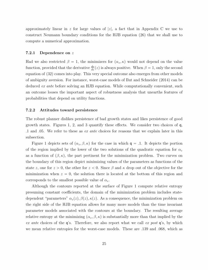
growth states. Figures 1, 2, and 3 quantify these effects. We consider two choices of q,
.1 and .05. We refer to these as ex ante choices for reasons that we explain later in this
subsection.
Figure 1 depicts sets of pαz, β, κq for the case in which q “ .1. It depicts the portion
of the region implied by the lower of the two solutions of the quadratic equation for αz
as a function of pβ, κq, the part pertinent for the minimization problem. Two curves on
the boundary of this region depict minimizing values of the parameters as functions of the
state z, one for z ą 0, the other for z ă 0. Since β and κ drop out of the objective for the
minimization when z “ 0, the solution there is located at the bottom of this region and
corresponds to the smallest possible value of αz.
Although the contours reported at the surface of Figure 1 compute relative entropy
presuming constant coefficients, the domain of the minimization problem includes state-
dependent “parameters” αzpzq, βpzq, κpzq. As a consequence, the minimization problem on
the right side of the HJB equation allows for many more models than the time invariant
parameter models associated with the contours at the boundary. The resulting average
relative entropy at the minimizing pαz, β, κq is substantially more than that implied by the
ex ante choices of the q’s. Therefore, we also report what we call ex post q’s, by which
we mean relative entropies for the worst-case models. These are .139 and .068, which as
25
anticipated, are larger than the ex ante value .1 and .05, respectively.
Figure 1: Set of alternative parameter values pαz, β, κq constrained by relative entropy. To
generate the parameter region, we set q “ .1 and plot only the lower portion of the set as
captured by αz. The red curve plots the chosen parameter configuration for z ă 0 and the
yellow curve for z ą 0. The z “ 0 solution is at the bottom of the region.
26
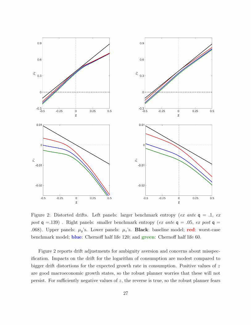
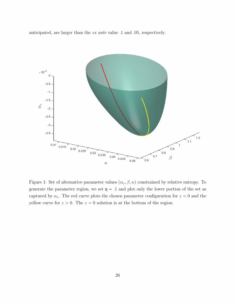
Figure 2: Distorted drifts. Left panels: larger benchmark entropy (ex ante q = .1, ex
post q =.139) . Right panels: smaller benchmark entropy (ex ante q = .05, ex post q =
.068). Upper panels: µy’s. Lower panels: µz’s. Black: baseline model; red: worst-case
benchmark model; blue: Chernoff half life 120; and green: Chernoff half life 60.
Figure 2 reports drift adjustments for ambiguity aversion and concerns about misspec-
ification. Impacts on the drift for the logarithm of consumption are modest compared to
bigger drift distortions for the expected growth rate in consumption. Positive values of z
are good macroeconomic growth states, so the robust planner worries that these will not
persist. For sufficiently negative values of z, the reverse is true, so the robust planner fears
27

persistence of bad growth states, concerns about alternatives within the set of benchmark
models. Adding concerns about misspecification of the set of benchmark models shifts the
drift of the growth state down, more in bad growth states than in good ones.
Figure 3: Distribution of Yt´Y0 under the baseline model and worst-case model for q = .1
and a Chernoff half life of 60 quarters. The black solid line depicts the median under the
baseline model and the associated gray shaded region gives the region within the .1 and .9
deciles. The red dashed line is the median under the worst-case model and the red shaded
region gives the region within the .1 and .9 deciles.
Figure 3 extrapolates impacts of the drift distortion on distributions of future consump-
tion growth over alternative horizons. It shows how the consumption growth distribution
adjusted for ambiguity aversion and misspecification tilts down relative to the baseline
distribution.
28

7.3 Uncertain dependence on the growth state
The growth state z affects the evolution of both consumption and the growth rate. We now
focus on the uncertainty on these terms only by restricting the constant terms to satisfy:
αz “ αz “ 0 and αy “ αy. Under these restrictions, average relative entropy simplifies to:
ε`
MR˘
“1
2
ˇ
ˇ
ˇ
ˇ
ˇ
σ´1
«
β ´ β
κ´ κ
ffˇ
ˇ
ˇ
ˇ
ˇ
2ˆ
|σz|2
2κ
˙
Consider an entropy set"
pβ, κq : ε`
MR˘
ď1
2q2
*
. (33)
For a given κ, to find the boundary of the entropy set (33) we solve a quadratic equation
for β and take the high β solution when κ ă κ and the low β solution when κ ą κ. We
obtain two functions β “ f´pκq for κ ă κ and β “ f`pκq for κ ą κ. The minimizing choice
of κ then solves:
.01df´
dκpκq ´
dυ
dzpzq “ 0
when z ă 0 and
.01df`
dκpκq ´
dυ
dzpzq “ 0
when z ą 0. Evidently, the worst-case κ depends on the value function.
The value function solves two coupled HJB equations, one for z ă 0 and another for
z ą 0. For z ă 0, the HJB equation is:
0 “minκ´δυpzq ` .01rαy ` f
´pκqzs ´ zκ
dυ
dzpzq `
1
2|σz|
2d2υ
dz2pzq
´1
2θ
”
.01 dυdzpzq
ı
σσ1
«
.01dυdzpzq
ff
.
There is an analogous equation for z ą 0. The discontinuity in worst-case benchmark
models at zero means that at z “ 0 the value function does not have a second derivative
at zero. We obtain two second-order differential equations in value functions and their
derivatives; these value functions coincide at z “ 0, as do their first-derivatives.
Figures 4 and 5 offer quantitative explorations of ambiguity aversion that focus exclu-
sively on the slope coefficients pβ, κq of the benchmark models.
29
Figure 4: Parameter contours for pβ, κq holding relative entropy fixed. The outer curve
q “ .1 and the inner curve q “ .05. The small diamond in the model depicts the baseline
model.
Figure 4 shows the boundaries for the q “ .1 and q “ .05 restrictions on relative entropy.
It is the lower segment of these contours that is targeted in the decision problem.
30

Figure 5: Distorted growth rate drifts. Left panel: larger benchmark entropy (q “ .1).
Right panel: smaller benchmark entropy (q “ .05). red: worst-case benchmark model;
blue: half life 120; and green: half life 60.
Figure 5 shows adjustments of the drifts due to ambiguity aversion and concerns about
misspecification of the benchmark models. Setting θ “ 8 silences concerns about about
misspecification of the benchmark models, all of which must be expressed through min-
imization over h. When we set θ “ `8, the implied worst-case benchmark model has
state dynamics that take the form of a threshold autoregression with a kink at zero. The
distorted drifts again show less persistence than does the baseline model for negative values
of z and more persistence for larger values of z. Activating a concern for misspecification
of the benchmark models by letting θ be finite shifts the drift as a function of the state
downwards, even more so for negative values of z than positive ones.
7.4 Commitment to a worst-case benchmark model
Partly to make contact with an alternative formulation proposed by Hansen and Sargent
(2016), we now alter timing protocols. Instead of pHt, Rtq being chosen simultaneously
each instant as depicted in HJB equation (20), a decision maker now confronts a single
benchmark model that has been chosen by a statistician in charge of choosing our R process.
The decision maker chooses an H process because he does not trust that benchmark model.
Until now, in choosing pH,Rq our decision maker has used discounted relative entropy.
31

We now assume that in choosing the R process, the statistician uses an undiscounted
counterpart of relative entropy. Recall that
limtÑ8
1
2tE
ˆż t
0
MRu |Ru|
2duˇ
ˇ
ˇF0
˙
“ limδÓ0
δ
2E
ˆż 8
0
expp´δuqMRu |Ru|
2duˇ
ˇ
ˇF0
˙
In choosing a baseline model, the statistician uses the δ Ó 0 measure and imposes the
restriction:
limδÓ0
δ
2E
„ż 8
0
expp´δuqMRu
`
|Ru|2´ ξu
˘
duˇ
ˇ
ˇF0
ď 0. (34)
This constraint is satisfied whenever |Rt|2 ď ξt but also for other models as well. The
process tξtu is specified exogenously. Relative entropy neighborhoods of interior martingales
are included in this set. Taking the δ Ó 0 limit eliminates the dependence on conditioning
information for a convex set of martingales MR.
To make these results comparable to earlier ones, we have the statistician construct a
set of models as follows
• Start with κ ă κ that is the smallest κ on one of the two curves in Figure 4.
• Let u “ κ´ κ. Then compute spuq by solving:
b “ mins
ˇ
ˇ
ˇ
ˇ
ˇ
σ´1
«
s
u
ffˇ
ˇ
ˇ
ˇ
ˇ
This construction assures that
$
&
%
pβ, κq :
ˇ
ˇ
ˇ
ˇ
ˇ
σ´1
«
β ´ β
κ´ κ
ffˇ
ˇ
ˇ
ˇ
ˇ
2
ď b2
,
.
-
contains the region inside the corresponding contour set in Figure 4. This leads us to
specify:
ξt “ b2|Zt|
2
in our computations.
We start with a date-zero perspective. The statistician uses the same instantaneous
utility function as the decision maker and takes a process of instantaneous utilities as
given. The statistician then uses a martingale relative to the baseline model to construct
32

a benchmark model by solving a continuous-time analogue of a control problem posed by
Petersen et al. (2000).
The decision maker discounts with δ ą 0 and accepts the statistician’s model as a
benchmark. Because he doubts it he makes a robustness adjustment of the type suggested
by Hansen and Sargent (2001). This problem is reminiscent of an optimal expectations
game formulated by Brunnermeier and Parker (2005). They formulate two-agent decision
problems in which one agent chooses beliefs using an undiscounted utility function while
the other agent takes those beliefs as fixed when evaluating alternative plans. Despite
formal connections between their work and ours, their work does not originate in concerns
about robustness.
An equilibrium for our robust planner game is particularly easy to compute because the
instantaneous utility is specified a priori. This allows us to first to solve the statistician
problem and then the decision maker’s problem.20
7.4.1 Statistician Problem
We solve the statistician problem first for a given δ and Lagrange multiplier `. The statis-
tician’s value function ς is quadratic in z and solves:
0 “minr´δςpz, δ, `q ` .01pαy ` βz ` σy ¨ rq `
dς
dzpz, δ, `q pαz ´ κz ` σz ¨ rq
`1
2|σz|
2 d2ς
dz2pz, δ, `q `
`
2
`
r ¨ r ´ b2z2˘
“´ δςpz, δ, `q ` .01pαy ` βzq `dς
dzpz, δ, `q pαz ´ κzq `
1
2|σz|
2 d2ς
dz2pz, δ, `q
´1
2`
”
.01 dςdzpz, δ, `q
ı
σσ1
«
.01dςdzpz, δ, `q
ff
´`b2z2
2
We take limits as δ gets small and set the multiplier ` to satisfy the relative entropy
constraint (34) by maximizing:
max`
limδÓ0
δςp¨, δ, `q.
Since in the small δ limit we do not discount the future, the maximizing multiplier `˚ does
not depend on z. See Appendix D for a characterization of the solution. The implied drift
20In a model with production, this two-step approach would no long apply.
33

adjustment used to represent the statisician’s benchmark model is
r˚ “ ι˚pzq “ ´1
`
˚
σ1
«
.01dςdzpz, 0, `˚q
ff
,
where we evaluate dςdzpz, 0, `˚q by computing a small δ limit of dς
dzpz, δ, `˚q. Since ς is quadratic
in z, the statistician’s worst-case benchmark model alters the probability distribution for
W to have a drift that is linear in z. This leads us to express the local dynamics for the
benchmark model as:
αy ` βz ` σy ¨ ι˚pzq “ α˚y ` β
˚z
αz ´ κz ` σz ¨ ι˚pzq “ α˚z ´ κ
˚z.
Evidently, here the worst-case benchmark model remains within our parametric class. Note
that this benchmark model is not a time-varying or state-dependent coefficient model, in
contrast to the situation found under the distinct section 7.3 setting.
7.4.2 Robust Control Problem
At date zero, the decision maker accepts the statistician’s model as a benchmark but
because he doubts it, he makes a robustness adjustment of the type suggested by Hansen
and Sargent (2001). Where the value function is mry ` ψpzqs, write the decision maker’s
HJB equation as21
0 “minh´δψpzq ` .01σy ¨ h` σz ¨ h
dψ
dzpzq `
θ
2h ¨ h
` .01`
α˚y ` β˚z˘
`dψ
dzpzq pα˚z ´ κ
˚zq `1
2|σz|
2d2ψ
dz2pzq
“ ´ δψpzq ` .01`
α˚y ` β˚z˘
`dψ
dzpzq pα˚z ´ κ
˚zq `1
2|σz|
2d2ψ
dz2pzq
´1
2θ
”
.01 dψdzpzq
ı
σσ1
«
.01dψdzpzq
ff
.
In this case we can say more. It is straightforward to show that ψpzq “ ψ0`ψ1z, where in
particular ψ1 solves:
0 “ ´δψ1 ` .01β˚ ´ ψ1κ˚
21As in earlier decision problems, we can omit m from the HJB equation because it multiplies all terms.
34

which implies
ψ1 “.01β˚
δ ` κ˚.
7.4.3 Results
The following composite22 worst-case model emerges from our statistician-decision maker
game:
h˚ “ η˚pzq “ ι˚pzq ´1
θσ1
«
.01dψdzpzq
ff
“ ι˚pzq ´1
θσ1
«
.01
ψ1
ff
In light of how we have formulated things, it is not surprising that the second term takes
a form found by Hansen et al. (2006). While this second term is constant in the present
example, the first term ι˚ is state dependent; η˚ remains within the parametric class of
benchmark models. Dynamic consistency prevails in the sense that if we ask the players
to re-assess their choices at some date t ą 0, each player would remain content with its
original choice.
We study values of θ chosen to match Chernoff half lives of 60 quarters and 120 quarters,
respectively. The statistician’s worst-case benchmark model has a linear drift for the state
variable but its slope is flatter than in the baseline model. It is also shifted downwards.
The decision maker’s concerns about misspecification of the statistician’s benchmark model
lead him to shift the worst-case drift as a function of the state variable downwards, while
keeping it parallel to that function in the benchmark model. Figure 6 illustrates these
effects.
22It is composed of worst-case R and H processes.
35
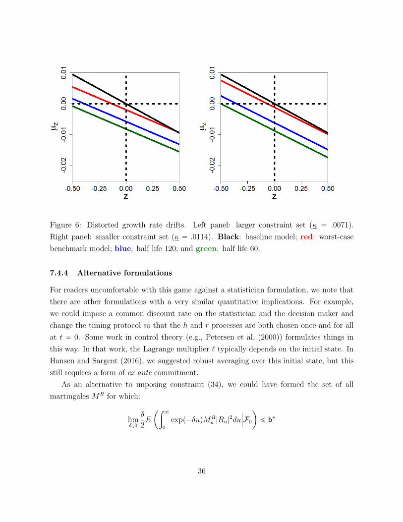
Figure 6: Distorted growth rate drifts. Left panel: larger constraint set (κ “ .0071).
Right panel: smaller constraint set (κ “ .0114). Black: baseline model; red: worst-case
benchmark model; blue: half life 120; and green: half life 60.
7.4.4 Alternative formulations
For readers uncomfortable with this game against a statistician formulation, we note that
there are other formulations with a very similar quantitative implications. For example,
we could impose a common discount rate on the statistician and the decision maker and
change the timing protocol so that the h and r processes are both chosen once and for all
at t “ 0. Some work in control theory (e.g., Petersen et al. (2000)) formulates things in
this way. In that work, the Lagrange multiplier ` typically depends on the initial state. In
Hansen and Sargent (2016), we suggested robust averaging over this initial state, but this
still requires a form of ex ante commitment.
As an alternative to imposing constraint (34), we could have formed the set of all
martingales MR for which:
limδÓ0
δ
2E
ˆż 8
0
expp´δuqMRu |Ru|
2duˇ
ˇ
ˇF0
˙
ď b˚
36

b˚ “ supR
limδÓ0
δ
2E
ˆż 8
0
expp´δuqMRu |Ru|
2duˇ
ˇ
ˇF0
˙
subject to |Rt|2 ď ξt. This modeling choice would have two consequences. First it would
result in an even larger set of martingales. Second, if applied to the present quantitative
example, the implied worst-case benchmark and worst-case models would entail adding
constant (and therefore state-independent) drifts to the Brownian motions.
8 Robust portfolio choice and pricing
In this section, we describe equilibrium prices that make a representative investor willing
to bear risks accurately described by baseline model (1) inspite of his concerns about model
misspecification. We construct equilibrium prices by appropriately extracting shadow prices
from the robust planning problem of section 4. We decompose equilibrium risk prices into
distinct compensations for bearing risk and for bearing model uncertainty. We begin by
posing the representative investor’s portfolio choice problem.
8.1 Robust investor portfolio problem
A representative investor faces a continuous-time Merton portfolio problem in which indi-
vidual wealth K evolves as
dKt “ ´Ctdt`KtιpZtqdt`KtAt ¨ dWt `KtπpZtq ¨ Atdt, (35)
where At “ a is a vector of chosen risk exposures, ιpxq is the instantaneous risk free rate
expressed, and πpzq is the vector of risk prices evaluated at state Zt “ z. Initial wealth
is K0. The investor discounts the logarithm of consumption and distrusts his probability
model.
Key inputs to a representative investor’s robust portfolio problem are the baseline model
(1), the wealth evolution equation (35), the vector of risk prices πpzq, and the quadratic
function ξ that defines the alternative explicit models that concern the representative in-
vestor.
Under a guess that the value function takes the form mυpzq ` m log k ` m log δ, the
37

HJB equation for the robust portfolio allocation problem is
0 “ maxa,c
minh,r´δmυpzq ´ δm log k ´ δm log δ ` δm log c´
mc
k`mιpzq
`mπpzq ¨ a`ma ¨ h´m|a|2
2`m
dυ
dzpzq pαz ´ κz ` σz ¨ hq
`m
2|σz|
2d2υ
dz2pzq `
ˆ
mθ
2
˙
|h´ r|2 (36)
subject to
r “nÿ
j“1
πjηjpzq, π P Π (37)
First-order conditions for consumption are
δ
c˚“
1
k,
which imply that c˚ “ δk, an implication that follows from the unitary elasticity of in-
tertemporal substitution. First-order conditions for a and h are
πpzq ` h˚ ´ a˚ “ 0 (38a)
a˚ ` θph˚ ´ r˚q `dυ
dzpzqσz “ 0. (38b)
These two equations determine a˚ and h˚´ r˚ as a function of πpzq and the value function
υ. We determine r˚ as a function of h˚ by solving:
minr
θ
2|h´ r|2.
subject to (37). Taken together, these determine pa˚, h˚, r˚q. We can appeal to arguments
like those of Hansen and Sargent (2008, ch. 7) to justify stacking first-order conditions as
a way to collect equilibrium conditions for the pertinent two-person zero-sum game.23
23If we were to use a timing protocol that allows the maximizing player to take account of the impactof its decisions on the minimizing agent, we would obtain the same equilibrium decision rules described inthe text.
38

8.2 Competitive equilibrium prices
We now impose logC “ Y as an equilibrium condition. We show here that the drift
distortion η˚ that emerges from the robust planner’s problem of section 5 determines prices
that a competitive equilibrium awards for bearing model uncertainty. To compute a vector
πpxq of competitive equilibrium risk prices, we find a robust planner’s marginal valuations
of exposures to the W shocks. We decompose that price vector into separate compensations
for bearing risk and for accepting model uncertainty.
Noting from the robust planning problem that the shock exposure vectors for logK and
Y must coincide implies
a˚ “ p.01qσy.
From (38b) and the solution for r˚,
h˚ “ η˚pzq,
where η˚ is the worst-case drift from the robust planning problem provided that we show
that υ “ υ, where υ is the value function for the robust planning problem. Thus, from
(38a), π “ π˚, where
π˚pzq “ p.01qσy ´ η˚pzq. (39)
Similarly, in the problem for a representative investor within a competitive equilibrium,
the drifts for logK and Y coincide:
´δ ` ιpzq ` rp.01qσy ´ η˚pzqs ¨ a˚ ´
.0001
2σy ¨ σy “ p.01qpαy ` βzq,
so that ι “ ι˚, where
ι˚pzq “ δ ` .01pαy ` βzq ` .01σy ¨ η˚pzq ´
.0001
2σy ¨ σy. (40)
We use these formulas for equilibrium prices to construct a solution to the HJB equation
of a representative investor in a competitive equilibrium by letting υ “ υ.
39

8.3 Local uncertainty prices
The equilibrium stochastic discount factor process for our robust representative investor
economy is
d logSt “ ´δdt´ .01´
αy ` βZt
¯
dt´ .01σy ¨ dWt `H˚t ¨ dWt ´
1
2|H˚
t |2dt. (41)
The components of the vector π˚pZtq given by (39) equal minus the local exposures to
the Brownian shocks. These are usually interpreted as local “risk prices,” but we shall
reinterpret them. Motivated by the decomposition
minus stochastic discount factor exposure “ .01σy ´H˚t ,
risk price uncertainty price
we prefer to think of .01σy as risk prices induced by the curvature of log utility and ´H˚t
as “uncertainty” prices induced by a representative investor’s doubts about the baseline
model. Here H˚t is state dependent.
8.4 Uncertainty prices over alternative investment horizons
In the context of our quantitative models, we now report the shock-price elasticities that
Borovicka et al. (2014) showed are horizon-dependent uncertainty prices of risk exposures.
Shock price elasticities describe the dependence of logarithms of expected returns on an
investment horizon. The logarithm of the expected return from a consumption payoff at
date t consists of two terms:
logE
˜
CtC0
ˇ
ˇ
ˇ
ˇ
ˇ
X0 “ x
¸
´ logE
«
St
ˆ
YtY0
˙
ˇ
ˇ
ˇ
ˇ
ˇ
X0 “ x
ff
. (42)
where logCt “ Yt. The first term is the expected payoff and the second is the cost of
purchasing that payoff. Notice that in our example, since imposed a unitary elasticity of
substitution:
St
ˆ
CtC0
˙
“MH˚
t
so the second term features the martingale computed to implement robustness.
To compute an elasiticity, we change locally the exposure of consumption to the un-
derlying Brownian motion compute the consequences for the expected return. From a
40

mathematical perspective, an important inputs into this calculation are Malliavin deriva-
tives. These derivatives measure how a shock at given date effects the consumption and the
stochastic discount factor processes. Both St and Ct depend on Brownian motion between
dates zero and t. We are particularly interested in the impact of date t shock on St and Ct.
Computing the derivative of the logarithm of the expected return given in (42) results in
E rDtCt|F0s
E rCt|F0s´ E
”
DtMH˚
t |F0
ı
where DtCt and MH˚
t denote the two dimensional vectors of Mallianvin derivatives ( with
respect to the two dimensional Brownian increment at date t for consumption and the
worst-case martingale.
Using the convenient formula familiar from other forms of differentiation
DtCt “ Ct pDt logCtq .
The Mallivian derivative of logCt “ Yt is the vector .01σy or the exposure vector logCt to
the Brownian increment dWt:
DtCt “ .01Ctσy,
and thusE rDtCt|F0s
E rCt|F0s“ .01σy
Similarly,
DtMHt “ H˚
t .
Therefore the term structure of prices that interest us are given by
.01σy ´ E”
MH˚
t H˚t |F0
ı
The first term is the familiar risk price for comsumption-based asset pricing. It is state
independent and contributes a (small) term that is independent of the horizon. In contrast,
for the second term the equilibrium drift distortion provides state dependent component and
its expectation under the distorted probability measure gives a time and state dependent
contribution to the term structure of uncertainty prices.24
24There are other horizon dependent elasticities that we could compute. For instance, we might look atthe impact of a shock at date zero on Ct and MH˚
t and trace out the impact of changing the horizon butkeeping the date of the shock fixed.
41
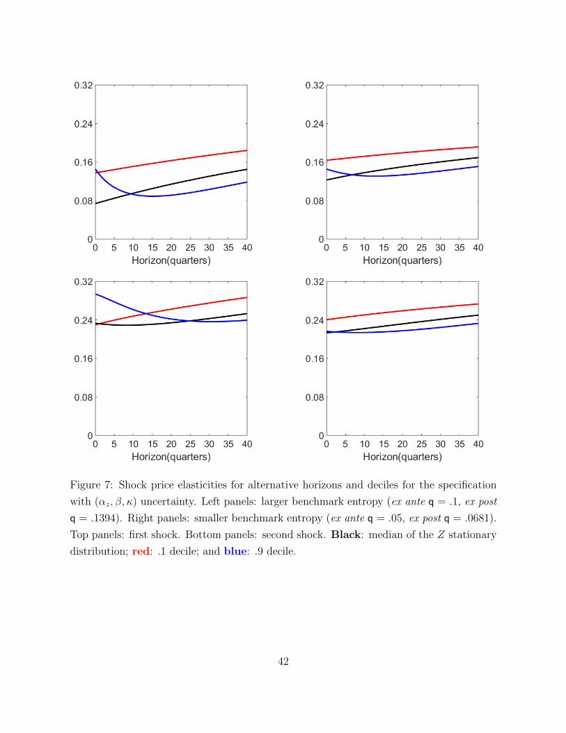
Figure 7: Shock price elasticities for alternative horizons and deciles for the specification
with pαz, β, κq uncertainty. Left panels: larger benchmark entropy (ex ante q = .1, ex post
q = .1394). Right panels: smaller benchmark entropy (ex ante q = .05, ex post q = .0681).
Top panels: first shock. Bottom panels: second shock. Black: median of the Z stationary
distribution; red: .1 decile; and blue: .9 decile.
42
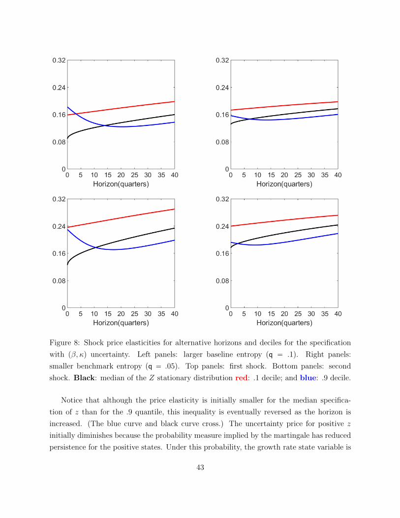
Figure 8: Shock price elasticities for alternative horizons and deciles for the specification
with pβ, κq uncertainty. Left panels: larger baseline entropy (q “ .1). Right panels:
smaller benchmark entropy (q “ .05). Top panels: first shock. Bottom panels: second
shock. Black: median of the Z stationary distribution red: .1 decile; and blue: .9 decile.
Notice that although the price elasticity is initially smaller for the median specifica-
tion of z than for the .9 quantile, this inequality is eventually reversed as the horizon is
increased. (The blue curve and black curve cross.) The uncertainty price for positive z
initially diminishes because the probability measure implied by the martingale has reduced
persistence for the positive states. Under this probability, the growth rate state variable is
43

expected to spends less time positive region. This is reflected in the smaller prices for the
.9 quantile than for the median over longer investment horizons. The endogenous nonlin-
earity in valuation has the uncertainty prices larger for negative values of z than positive
for longer investment horizons, but not necessarily for very short ones.
Figure 9: Shock price elasticities for alternative horizons and deciles for the specification
with pβ, κq uncertainty. Left panels: larger constraint set (κ “ .0071). Right panels:
smaller constraint set (κ “ .0114). Top panels: first shock. Bottom panels: second shock.
Black: median of the Z stationary distribution red: .1 decile; and blue: .9 decile.
44
We have structured our quantitative examples to investigate a particular mechanism
for generating fluctuations in uncertainty prices from statistically plausible amounts of
uncertainty. We infer parameters of the baseline model for these examples solely from time
series of macroeconomic quantities, thus completely ignoring asset prices during calibration.
As a consequence, we do not expect to track closely the high frequency movements in
financial markets. By limiting our empirical inputs, we respect concerns that Hansen (2007)
and Chen et al. (2015) expressed about using asset market data to calibrate macro-finance
models that assign a special role to investors’ beliefs about the future asset prices.25
9 Concluding remarks
This paper formulates and applies a tractable model of the effects on equilibrium prices
of exposures to macroeconomic uncertainties. Our analysis uses models’ consequences for
discounted expected utilities to quantify investors’ concerns about model misspecification.
We characterize the effects of concerns about misspecification of a baseline stochastic pro-
cess for individual consumption as shadow prices for a planner’s problem that supports
competitive equilibrium prices.
To illustrate our approach, we have focused on the growth rate uncertainty featured
in the “long-run risk” literature initiated by Bansal and Yaron (2004). Other applications
seem natural. For example, the tools developed here could shed light on a recent public
debate between two groups of macroeconomists, one prophesizing secular stagnation be-
cause of technology growth slowdowns, the other dismissing those pessimistic forecasts.
The tools that we describe can be used, first, to quantify how challenging it is to infer
persistent changes in growth rates, and, second, to guide macroeconomic policy design in
light of available empirical evidence.
Specifically, we have produced a model of the log stochastic discount factor whose
uncertainty prices reflect a robust planner’s worst-case drift distortions η˚. We have argued
that these drift distortions should be interpreted as prices of model uncertainty. The
dependency of these uncertainty prices η˚ on the growth state z is shaped partly by the
25Hansen (2007) and Chen et al. (2015) describe situations in which it is the behavior of rates of returnon assets that, through the cross-equation restrictions, lead an econometrician to make inferences aboutthe behavior of macroeconomic quantities like consumption that are much more confident than can bemade from the quantity data alone. That opens questions about how the investors who are supposedlyputting those cross-equation restrictions into returns came to know those quantity processes before theyobserved returns.
45

alternative parametric models that the decision maker entertains. In this way, our theory of
state dependence in uncertainty prices is all about how our robust investor responds to the
presence of the alternative parametric models among a huge set of unspecified alternative
models that also concern him.
It is worthwhile comparing this paper’s way of inducing time varying prices of risk with
three other macro/finance models that also get them. Campbell and Cochrane (1999) pro-
ceed in the standard rational expectations single-known-probability-model tradition and so
exclude any fears of model misspecification from the mind of their representative investor.
They construct a history-dependent utility function in which the history of consumption
expresses an externality. This history dependence makes the investor’s local risk aversion
depend in a countercyclical way on the economy’s growth state. Ang and Piazzesi (2003)
use an exponential quadratic stochastic discount factor in a no-arbitrage statistical model
and explore links between the term structure of interest rates and other macroeconomic
variables. Their approach allows movements in risk prices to be consistent with historical
evidence without specifying an explicit general equilibrium model. A third approach intro-
duces stochastic volatility into the macroeconomy by positing that the volatilities of shocks
driving consumption growth are themselves stochastic processes. A stochastic volatility
model induces time variation in risk prices via exogenous movements in the conditional
volatilities impinging on macroeconomic variables.
In Hansen and Sargent (2010), countercyclical uncertainty prices are driven by a rep-
resentative investor’s robust model averaging. The investor carries along two difficult-to-
distinguish models of consumption growth, one asserting i.i.d. log consumption growth,
the other asserting that the growth in log consumption is a process with a slowly mov-
ing conditional mean. The investor uses observations on consumption growth to update a
Bayesian prior over these two models, starting from an initial prior probability of .5. The
prior wanders over a post WWII sample period, but ends where it started. Each period,
the Hansen and Sargent representative investor expresses his specification distrust by pes-
simistically exponentially twisting a posterior over the two baseline models. That leads the
investor to interpret good news as temporary and bad news as persistent, causing him to
put countercyclical uncertainty components into equilibrium “risk” prices. Learning occurs
in their analysis because the parameterized set of baseline models are time invariant and
hence learnable. The decision makers in their analysis confront dynamic consistency by
playing a game against future versions of themselves.
In this paper, we propose a different way to make uncertainty prices vary in a qual-
46

itatively similar way. We exclude learning and instead consider alternative models with
parameters whose future variations cannot be inferred from historical data. These time-
varying parameter models differ from the decision maker’s baseline model, a fixed parameter
model whose parameters can be well estimated from historical data. The alternative models
include ones that allow parameters persistently to deviate from those of the baseline model
in statistically subtle and time-varying ways. In addition to this particular class of alter-
native models, the decision maker also includes other statistical specifications in the set of
models that concern him. The robust planner’s worst-case model responds to these forms
of model ambiguity partly by having more persistence in bad states and less persistence in
good states. Adverse shifts in the shock distribution that drive up the absolute magnitudes
of uncertainty prices were also present in some of our earlier work (for example, see Hansen
et al. (1999) and Anderson et al. (2003)). In this paper, we induce state dependence in
uncertainty prices in a different way, namely, by specifying a set of alternative models to
capture concerns about the baseline model’s specification of persistence in consumption
growth.
Relative to rational expectations models, models of robustness and ambiguity aversion
bring new parameters. In this paper, we extend work by Anderson et al. (2003) that cali-
brated those additional parameters by exploiting connections between models of statistical
model discrimination and our way of formulating robustness. We build on mathematical
formulations of Newman and Stuck (1979), Petersen et al. (2000), and Hansen et al. (2006).
We pose an ex ante robustness problem that pins down a robustness penalty parameter θ
by linking it to an asymptotic measure of statistical discrimination between models. This
asymptotic measure allows us to quantify a half-life for reducing the mistakes in selecting
between competing models based on historical evidence. A large statistical discrimination
rate implies a short half-life for reducing discrimination mistake probabilities. Anderson
et al. (2003) and Hansen (2007) had studied the connection between conditional discrimi-
nation rates and uncertainty prices that clear security markets. By following Newman and
Stuck (1979) and studying asymptotic discrimination rates, we link statistical discrimina-
tion half-lives to calibrated equilibrium uncertainty prices.
47

Appendices
A Operationalizing Chernoff entropy
In this appendix we show how to compute entropies for parametric models of the form (24).
Because the H’s associated with them take the form
Ht “ ηpZtq,
these alternative models are Markovian.
Given the Markov structure of both models, we compute Chernoff entropy by using an
eigenvalue approach of Donsker and Varadhan (1976) and Newman and Stuck (1979). We
start by computing the drift of`
MHt
˘sgpZtq for 0 ď s ď 1 at t “ 0:
rGpsqgspzq .“p´s` s2q
2|ηpzq|2gpzq ` sgpzq1σ ¨ ηpzq
´ g1pzqκz `g2pzq
2|σ|2,
where rGpsqgspxq is the drift given that Z0 “ z. Next we solve the eigenvalue problem
rGpsqsepz, sq “ ´ρpsqepz, sq,
whose eigenfunction epz, sq is the exponential of a quadratic function of z. We compute
Chernoff entropy numerically by solving:
χpMHq “ max
sPr0,1sρpsq.
To deduce a corresponding equation for log e, notice that
plog eq1pzq “e1pzq
epzq
and
plog eq2pzq “e2pzq
epzq´
„
e1pzq
epzq
2
.
48

For a positive g
rGpsqgspzqgpzq
.“p´s` s2q
2|ηpzq|2 ` splog gq1pzqσ ¨ ηpzq ´ plog gq1pzqκz
`log g2pzq
2|σ|2 `
rlog g1pzqs2
2|σ|2. (43)
Using formula (43), define
“
Gpsq log g‰
pzq “rGpsqgspzq
gpzq.
Then we can solve“
Gpsq log e‰
pz, sq “ ´ρpsq
for log e to compute the positive eigenfunction e.
These calculations allow us numerically to compute Chernoff entropies:
d log Yt “ p.01q pαy ` βZtq dt` p.01qσy ¨ dĂWt
dZt “ αzdt´ κZtdt` σz ¨ dĂWt.
1. Input values of κ, β, αy, and αz. Construct the implied hpzq “ η1z ` η0 by solving;
«
αy ´ αy
αz ´ αz
ff
“ ση0
«
β ´ β
κ´ κ
ff
“ ση1
for η1 and η0.
2. For a given s, construct ζ0, ζ1, ζ2, κ, β, φ, and µ from:
p´s` s2q|η0 ` η1z|
2“ ´
`
ζ0 ` 2ζ1z ` ζ2z2˘
κ “ p1´ sqκ` sκ
β “ p1´ sqβ ` sβ
49

µy “ p1´ sqµy ` sµy
µz “ p1´ sqµz ` sµz
3. Solve
´ρpsq “ ´1
2
`
ζ0 ` 2ζ1x` ζ2z2˘
` pµz ´ zκqplog eq1pzq
`plog eq2pzq
2|σz|
2`rplog eq1pzqs2
2|σz|
2
where log epz, sq “ λ1z `12λ2z
2. Thus,
λ2 “κ´
b
pκq2 ` ζ2|σz|2
|σz|2.
Given λ2, λ1 solves
´ζ1 ´ κλ1 ` λ1λ2|σz|2` µzλ2 “ 0
or
λ1 “ζ1 ´ µzλ2
λ2|σz|2 ´ κ“ ´
ζ1 ´ µzλ2b
pκq2 ` ζ2|σz|2.
Finally,
ρpsq “1
2ζ0 ´
1
2|σz|
2λ2 ´1
2|σz|
2pλ1q
2´ µzλ1.
4. Repeat for alternative s’s and maximize ρpsq as a function of s.
B Statistical calibration
We fit a trivariate VAR with the following variables:
log Yt`1 ´ log Yt
logGt`1 ´ log Yt`1
logDt`1 ´ log Yt`1
where Gt is the sum of corporate profits and proprietors’ income and Dt is personal income.
Provided that the VAR has stable coefficients, this is a co-integrated system. All three
50

time series have stationary increments, but there one common martingale process. The
shock to this process is identified as the only one with long-term consequences. We set
αz “ 0 and βy “ 1. For the remaining parameters we:
i) fit a VAR with a constant and four lags of the first variable and five of the other two;
ii) compute the implied mean for for log Yt`1 ´ log Yt and set this to αy;
iii) compute the state dependent component of the expected long-term growth rate by
calculating:
log Y pt “ lim
jÑ8E plog Yt`j ´ log Yt ´ jαy|Ftq
implied by the VAR estimates, to compare to the counterpart calculation in the
continuous-time model:
Zpt “ lim
jÑ8E plog Yt`j ´ log Yt ´ jα|Ztq “
1
κZt.
iv) compute the implied autoregressive coefficient for tlog Y pt u in the discrete-time speci-
fication using the VAR parameter estimates and equate this coefficient to 1´ κ.
v) compute the VAR implied covariance matrix for the one-step-ahead forecast error for
tlog Y pu, the direct shock to consumption and equate this to
«
pσyq1
1κpσzq
1
ff
”
pσyq1κpσzq
ı
where we achieve identification of σz and σy by imposing a zero restriction on the
second entry of σy and positive signs on the first coefficient of σy and on the second
coefficient of σz.
C Solving the ODE’s
The value function is approximately linear in the state variable for large |z|. This gives
a good boundary Neumann boundary condition to use in an approximation in which z is
restricted to a compact interval that includes z “ 0. To deduce this boundary restriction
51

solve:
p´δ ´ κqν ` .01β “ 0
νBε
Bβpαz, β, κq ` .01
Bε
Bκpαz, β, κq “0
Bε
Bαzpαz, β, κq “0
εpαz, β, κq ´1
2q2“0
for pν, αz, β, κq. The first equation is the derivative of the value function for constant coeffi-
cients, putting aside the minimization. The next two equations are large z approximations
to the first-order conditions (32). The last equation targets the boundary of the feasible
region for the parameter values pαz, β, κq. Notice that the last two equations imply that
the αz minimizes the quadratic function and is a zero of it. Thus the discriminate of this
associated quadratic equation is zero. This gives a function of κ and β alone along with a
formula for αz “ fpβ, κq. There will be multiple ways to make the discriminate zero, and
we need to pick the one corresponding to low κ and high β for z ăă 0 in the final solution.
We proceed analogously for z ąą 0 by selecting the high κ and low β solution.
Consider now the special case in which αz “ αz. We proceed as before except that we
drop the third equation.
D Statistician value function
Recall that we studied a two-agent game: a statistician that chooses a baseline model, and
a decision maker who doesn’t fully trust the baseline model. In this appendix we provide
some formulas for the statistician value function.
The HJB equation for the statistician is:
0 “´ δςpz, δ, `q ` .01pαy ` βzq `dς
dzpz, δ, `q pαz ´ κzq `
1
2|σz|
2 d2ς
dz2pz, δ, `q
´1
2`
”
.01 dςdzpz, δ, `q
ı
σσ1
«
.01dςdzpz, δ, `q
ff
´`b2z2
2
52

Guess that that the value function is quadratic
ς pz, δ, `q “ ´1
2
“
ς2pδ, `qz2` 2ς1pδ, `qz ` ς0pδ, `q
‰
which implicitly depends on `. The implied worst-case benchmark distortion is
ι˚pzq “ ´1
`r.01σy ´ σzς2pδ, `qz ´ σzς1pδ, `qs .
We solve for ς2, ς1, and ς0 by matching the coefficients for z2, z and the constant terms,
respectively. Solving first for ς2 collection the z2 terms. This results in the quadratic
equation of the form Apς2q2 `Bς2 ` C “ 0 where
A “ ´1
2`|σz|
2
B “ κ`δ
2
C “ ´`
2b2.
Then
ς2pδ, `q “´B `
?B2 ´ 4AC
2A
“ `
»
–
δ ` 2κ´b
pδ ` 2κq2 ´ 4 |σz|2 b2
2 |σz|2
fi
fl
ς1pδ, `q “2
»
–
´.01β ` αzς2pδ, `q ´.01`pσy ¨ σzq ς2pδ, `q
δ `b
pδ ` 2κq2 ´ 4 |σz|2 b2
fi
fl
ς0pδ, `q “1
δ
„
´.02αy ` 2αzς1pδ, `q ` |σz|2 ς2pδ, `q `
1
`|.01σy ´ σzς1pδ, `q|
2
To solve the undiscounted problem, we now compute three limits:
ς2p0, `q “ limδÓ0
ς2pδ, `q “ `
»
–
κ´b
pκq2 ´ |σz|2 b2
|σz|2
fi
fl
53

ς1p0, `q “ limδÓ0
ς1pδq “
»
–
´.01β ` αzς2p0, `q ´.01`pσy ¨ σzq ς2p0, `q
b
pκq2 ´ |σz|2 b2
fi
fl
limδÓ0
δς0pδ, `q “
„
´.02αy ` 2αzς1p0, `q ` |σz|2 ς2p0, `q `
1
`|.01σy ´ σzς1p0, `q|
2
.
We compute ` by solving:
max`
limδÓ0´δς0pδ, `q.
54
References
Anderson, Evan W., Lars Peter Hansen, and Thomas J. Sargent. 1998. Risk and Robustness
in Equilibrium. Available on webpages.
———. 2003. A Quartet of Semigroups for Model Specification, Robustness, Prices of Risk,
and Model Detection. Journal of the European Economic Association 1 (1):68–123.
Ang, Andrew and Monika Piazzesi. 2003. A No-Arbitrage Vector Autoregression of the
Term Structure Dynamics with Macroeconomic and Latent Variables. Journal of Mon-
etary Economics 50:745–787.
Bansal, Ravi and Amir Yaron. 2004. Risks for the Long Run: A Potential Resolution of
Asset Pricing Puzzles. Journal of Finance 59 (4):1481–1509.
Berger, James O. 1994. An Overview of Robust Bayesian Analysis (with discussion). Test
3 (1):5–124.
Bhandari, Anmol. 2014. Doubts, Asymmetries, and Insurance. University of Minnesota.
Borovicka, Jaroslav, Lars Peter Hansen, and Jose A. Scheinkman. 2014. Shock Elasticities
and Impulse Response Functions. Mathematics and Financial Economics 8 (4):333–354.
Brunnermeier, Markus K. and Jonathan A. Parker. 2005. Optimal Expectations. American
Economic Review 95 (4):1092–1118.
Campbell, John Y. and John Cochrane. 1999. Force of Habit: A Consumption-Based Expla-
nation of Aggregate Stock Market Behavior. Journal of Political Economy 107 (2):205–
251.
Chamberlain, Gary. 2000. Econometric Applications of Maxmin Expected Utility. Journal
of Applied Econometrics 15 (6):625–644.
Chen, Hui, Winston Wei Dou, and Leonid Kogan. 2015. Measuring the ‘Dark Matter’ in
Asset Pricing Models. MIT Sloan School of Management.
Chen, Zengjing and Larry Epstein. 2002. Ambiguity, Risk, and Asset Returns in Continuous
Time. Econometrica 70:1403–1443.
55

Chernoff, Herman. 1952. A Measure of Asymptotic Efficiency for Tests of a Hypothesis
Based on the Sum of Observations. Annals of Mathematical Statistics 23 (4):pp. 493–507.
Donsker, Monroe E. and S. R. Srinivasa Varadhan. 1976. On the Principal Eigenvalue
of Second-Order Elliptic Differential Equations. Communications in Pure and Applied
Mathematics 29:595–621.
Epstein, Larry G. and Martin Schneider. 2003. Recursive multiple-priors. Journal of
Economic Theory 113 (1):1–31.
Fudenberg, Drew and David K. Levine. 2009. Self-confirming Equilibrium and the Lucas
Critique. Journal of Economic Theory 144 (6):2354–2371.
Good, I. J. 1952. Rational Decisions. Journal of the Royal Statistical Society. Series B
(Methodological) 14 (1):pp. 107–114.
Hansen, L. P., J. C. Heaton, and N. Li. 2008. Consumption Strikes Back?: Measuring Long
Run Risk. Journal of Political Economy .
Hansen, Lars P. and Thomas J. Sargent. 2016. Sets of Models and Prices of Uncertainty.
NBER Working Papers 22000, National Bureau of Economic Research, Inc.
Hansen, Lars Peter. 2007. Beliefs, Doubts and Learning: Valuing Macroeconomic Risk.
American Economic Review 97 (2):1–30.
Hansen, Lars Peter and Massimo Marinacci. 2016. Ambiguity Aversion and Model Mis-
specification: An Economic Perspective. Statistical Science Forthcoming.
Hansen, Lars Peter and Thomas Sargent. 2010. Fragile beliefs and the price of uncertainty.
Quantitative Economics 1 (1):129–162.
Hansen, Lars Peter and Thomas J. Sargent. 2001. Robust Control and Model Uncertainty.
American Economic Review 91 (2):60–66.
———. 2008. Robustness. Princeton, New Jersey: Princeton University Press.
Hansen, Lars Peter, Thomas J. Sargent, and Jr. Tallarini, Thomas D. 1999. Robust Per-
manent Income and Pricing. The Review of Economic Studies 66 (4):873–907.
56
Hansen, Lars Peter, Thomas J. Sargent, Gauhar A. Turmuhambetova, and Noah Williams.
2006. Robust Control and Model Misspecification. Journal of Economic Theory
128 (1):45–90.
Ilut, Cosmin L. and Martin Schneider. 2014. Ambiguous Business Cycles. American Eco-
nomic Review 104 (8):2368–99.
James, Matthew R. 1992. Asymptotic analysis of nonlinear stochastic risk-sensitive control
and differential games. Mathematics of Control, Signals and Systems 5 (4):401–417.
Karantounias, Anastasios G. 2013. Managing pessimistic expectations and fiscal policy.
Theoretical Economics 8 (1).
Lucas, Jr, Robert E. 1978. Asset Prices in an Exchange Economy. Econometrica
46 (6):1429–45.
Maccheroni, Fabio, Massimo Marinacci, and Aldo Rustichini. 2006a. Ambiguity Aver-
sion, Robustness, and the Variational Representation of Preferences. Econometrica
74 (6):1447–1498.
———. 2006b. Dynamic Variational Preferences. Journal of Economic Theory 128:4–44.
Mehra, Rajnish and Edward C. Prescott. 1985. The equity premium: A puzzle. Journal of
Monetary Economics 15 (2):145–161.
Miao, Jianjun and Alejandro Rivera. 2016. Robust Contracts in Continuous Time. Econo-
metrica 84 (4):1405–1440.
Newman, C. M. and B. W. Stuck. 1979. Chernoff Bounds for Discriminating between Two
Markov Processes. Stochastics 2 (1-4):139–153.
Petersen, I.R., M.R. James, and P. Dupuis. 2000. Minimax optimal control of stochastic
uncertain systems with relative entropy constraints. Automatic Control, IEEE Transac-
tions on 45 (3):398–412.
Sargent, Thomas J. 1999. The Conquest of American Inflation. Princeton, New Jersey:
Princeton University Press.
Watson, James and Chris Holmes. 2016. Approximate Models and Robust Decisons. Sta-
tistical Science Forthcoming.
57