sourcing through intermediaries: the role of...
TRANSCRIPT
Sourcing through Intermediaries:
The Role of Competition
Elodie AdidaSchool of Business Administration, University of California at Riverside, [email protected]
Nitin BakshiManagement Science and Operations, London Business School, [email protected]
Victor DeMiguelManagement Science and Operations, London Business School, [email protected]
We study the joint impact of horizontal and vertical competition in retailer-driven global supply chains
with intermediaries. We show that, as a consequence of the retailers leading, intermediaries prefer products
for which the supplier base (existing production capacity) is neither too narrow nor too broad. We also find
that the “right” balance of horizontal and vertical competition can entirely offset the double marginalization
effect caused by the existence of an additional intermediary tier, and thus lead to supply chain efficiency.
On accounting for intermediaries’ private information about the supply side, we find that it has the indirect
effect of attenuating competition between retailers, who may therefore be better off (under some scenarios)
relative to the case with complete information. Finally, we show how the classical transaction cost rationale
for the existence of intermediaries can be incorporated to our competition framework, and find that retailers
are more likely to use intermediaries when manufacturing costs increase, and that the threat that retailers
may procure directly from the suppliers pushes intermediaries to expand their supply base.
Key words : Supply chain, vertical and horizontal competition, Stackelberg leader, intermediation.
History : May 6, 2014
1. Introduction
For several decades, intense competition has driven retailers in developed countries to source prod-
ucts from low-cost international suppliers. For commodity-type products, which tend to have long
life cycles, the retailer’s in-house procurement department often establishes a long-term relation-
ship with one or more suitable suppliers that can fulfill demand. For specialized products such as
fashion apparel, fashion shoes, toys, and housewares, however, retailers typically rely on interme-
diaries. These industries are characterized by high frequency of new product introduction coupled
with short product life cycles, and thus require the use of a large and complex network of low-
cost international suppliers. Under these circumstances, retailers generally find it economical to
2 Adida, Bakshi, and DeMiguel: Sourcing through Intermediaries
outsource the maintenance of this network to intermediaries with deep knowledge of the product
market and international supplier base. For instance, sourcing through trading companies is typical
in fashion apparel (Masson et al. 2007, Ha-Brookshire and Dyer 2008, and Purvis et al. 2013).
Specifically, [Masson et al. 2007, p. 247] study several UK clothing retailers and find that: “With
the increasing number of new products introduced more frequently as well as the smaller volumes
per product, the pool of skills required for clothing manufacturing is becoming more complex,
requiring a larger global network of suppliers every season. For most retailers, developing a global
sourcing network was not effective. We found that the common norm was simply for the retailers
to make use of third party indirect sourcing import/export agencies or what many choose to call
intermediaries.”
When an intermediary receives an order from a retailer, it identifies from its supplier base the
firms with appropriate expertise and spare capacity to fulfill the order, and charges a margin to the
retailer for its mediation. In addition, intermediaries often offer a variety of network coordination
services such as procuring raw material; monitoring of compliance with ethical, safety, and quality
standards; and arranging logistics and shipping.
This form of intermediation has recently received media attention due to the increasing globaliza-
tion of supply chains and the resulting prominence of mega intermediaries such as Hong-Kong-based
Li & Fung Limited (The Telegraph 2012). However, most intermediaries or trading companies are
small, yet they play a critical role in facilitating procurement in international supply chains; see
Rauch [2001]. For instance, Hsing [1999] explains that trading companies were the predominant
conduit for fashion shoes produced during Taiwan’s manufacturing boom between the mid-1970s
and the mid-1980s, and that “most Taiwan trading companies were small, with an average of seven
employees”.
Vertical and horizontal competition are inherent aspects of global supply chains with interme-
diaries. By definition, when a retailer outsources procurement to an intermediary, the relationship
between them is one of vertical competition. Similarly, intermediaries and suppliers engage in ver-
tical competition—indeed Hsing [1999] argues that intermediaries like to keep their distance with
suppliers so that retailers feel comfortable delegating quality control to them. Horizontal com-
petition is also rife. Small trading companies are subject to fierce horizontal competition; e.g.,
[Hsing 1999, p. 112] explains that “a manufacturer usually had more than one partner trading
company”, and [Ha-Brookshire and Dyer 2008, p. 11] document that industry executives describe
the environment of US apparel import intermediaries as one of “deadly competition”. Likewise,
retailers, which often compete for consumer demand, compete also to source from the same set of
intermediaries; e.g., [Masson et al. 2007, p. 247] mention that intermediaries “work for multiple
customers”.
Competition is clearly a prominent aspect of global supply chains with intermediaries, yet most
of the existent literature has by-and-large ignored this aspect and focused instead on identifying
Adida, Bakshi, and DeMiguel: Sourcing through Intermediaries 3
rationales for the existence of intermediaries. In this paper, we aim to address this gap in the
literature by studying the joint impact of horizontal and vertical competition on the performance
of a given supply chain with intermediaries. To do so, we model a three-tier supply chain, where
the middle tier consists of a set of intermediaries who compete in quantities to mediate between the
other two tiers, which consist of quantity-competing retailers and capacity-constrained suppliers.
A critical difference between our model and most existing models of multi-tier supply-chain
competition is that our model portrays the retailers as Stackelberg leaders. Portraying retailers
as followers is reasonable for many real-world supply chains (e.g., Dell and Coca-Cola may well
lead the supply chains for distribution of their products), but may not be realistic in the context
of intermediation firms that mediate between retailers in industries such as fashion apparel or
shoes and low-cost international suppliers. For instance, fashion retailers continuously monitor
market trends and generate orders as a response to these rapidly changing trends. Depending on
the specific order, the intermediary thereafter selects the suppliers with the technical capability
and spare capacity to fulfill demand. In other words, intermediaries orchestrate retailer-driven
global supply chains as a response to a specific order from a retailer facing incidental demand; see
Masson et al. [2007] and Knowledge@Wharton [2007]. Chronologically, the retailer order precedes
the orchestration of the supply chain, and thus it makes sense to portray the retailers as leaders.
We provide a complete analytical characterization of the symmetric supply chain equilibrium,
and use the closed-form expressions to answer four research questions. First, how does the compet-
itive environment affect the profits of retailers and intermediaries? In particular, can the retailers
leverage their leadership position to increase their market power and seize a large share of the
overall supply chain profits? And, under which competitive circumstances can intermediaries retain
a substantial share of the overall profits? Second, how does the presence of an intermediary tier
affect the efficiency of the decentralized supply chain? The literature shows that intermediaries
help retailers to overcome informational and transactional barriers, and thus they generally help
to improve the overall performance of global supply chains. Nevertheless, the question remains
whether the vertical competition established between retailers and intermediaries in global sup-
ply chains results in the double marginalization effect first identified by Spengler [1950], and thus
brings an element of inefficiency. Third, can intermediaries exploit their private information about
the supply side to alter their relative bargaining position with respect to the retailers? As men-
tioned above, intermediaries use their knowledge of the international supplier base to help retailers
overcome their informational barriers, but as noted in Babich and Yang [2014], when suppliers have
private information and procurement service providers (PSPs) are better informed than buyers,“it
is not obvious that PSPs would share benefits of better information with the buyer.” We con-
sider the case where intermediaries help retailers to identify suitable suppliers, but they withhold
information about the suppliers’ cost function, in an attempt to improve their bargaining position.
Fourth, how does competition affect the well-documented transactional benefits of intermediation?
To answer this question, we consider a variant of our model where retailers have the option to

4 Adida, Bakshi, and DeMiguel: Sourcing through Intermediaries
deal directly with the suppliers (without an intermediary) provided they are willing to pay a fixed
transaction cost per supplier, and study how competition affects the retailers decision to either
source directly or through intermediaries.
With respect to the impact of competition on retailer and intermediary profits, we find that the
intermediary profits are unimodal with respect to the number of suppliers in its base. This is
in direct contrast with the insight from existing models of supply chain competition, in which
suppliers lead. Based on that literature, one might have expected that the larger the supplier
base, the larger the market power of the intermediaries and thus the larger their profits. This
intuition does bear out when the size of the supplier base is “small”. However, in a world where
retailers lead, when the supplier base is “large enough”, we show that the weakness of the suppliers
becomes the weakness of the intermediaries, and the retailers exploit their leadership position to
increase their market power and retain greater supply chain profits. A crucial implication of this
result is that intermediaries in retailer-driven global supply chains prefer products for which the
supplier base (existing production capacity) is neither too narrow nor too broad, because (ceteris
paribus) products for which there is an intermediate production capacity available generate larger
intermediary profits. The result also offers some insight into how the financial performance of
trading companies, and consequently of economies reliant on this sector, depends on the available
production capacity. This capacity is a function of various economic and environmental factors.
For instance, Barrie [2013] reports a shortfall in available capacity for 2013 in the fashion apparel
sector, whereas Zhao [2013] points to endemic overcapacity in the Chinese fashion industry during
1980s and 1990s. Our analysis shows that intermediary profits will be squeezed in either of these
two eventualities; that is, in case of shortfall or excess in available capacity.
With respect to supply chain efficiency, we observe that the presence of an additional tier of
intermediaries does not necessarily introduce an element of inefficiency to the decentralized sup-
ply chain; that is, the aggregate supply chain profits in the decentralized three-tier chain is not
necessarily smaller than that in the centralized (integrated) supply chain. The classic result on
double marginalization would have suggested otherwise (Spengler 1950). However, the differentiat-
ing feature of our analysis is that, along with vertical competition, we simultaneously account for
horizontal competition. It is well known that the relative bargaining strength of players in a verti-
cal relationship significantly determines the extent of double marginalization. Further, increasing
the number of within-tier competitors reduces a specific player’s bargaining power in the vertical
interaction. Such adjustments to competitive intensity may be carried out at each tier. We find
that there always exists an appropriate balance between horizontal and vertical competition that
completely offsets the effect of double marginalization, and leads to supply chain efficiency. An
implication of this result is that regulators may try and improve the efficiency of global supply
chains by taking measures to encourage a healthy level of competition at each of the three tiers.
Our analysis demonstrates, however, that in order for regulatory intervention to be successful, it
must be carefully tailored to the structure of the supply chain in question.
Adida, Bakshi, and DeMiguel: Sourcing through Intermediaries 5
We mentioned earlier that the retailers exploit their leadership position to increase their market
power with respect to the intermediaries. This leads one to wonder whether intermediaries can
exploit their private information about the supplier’s cost function to extract greater rents. To
answer this question, we consider the case when the intermediaries know whether the supply
sensitivity to price is high or low, but the retailers believe the sensitivity follows a certain prior
distribution—in our model, higher sensitivity of supply corresponds to a steeper marginal cost
function for the suppliers. We then characterize the impact of asymmetric information on both the
expected and the realized equilibrium profits.1 The comparison of the expected equilibrium profits
shows that on average the intermediaries are indeed able to exploit their private information at
the expense of the retailers.
The comparison of the realized equilibrium profits, however, shows that the realized profits of both
intermediaries and retailers could be higher or lower depending on the realized supply sensitivity.
In particular, when the realized sensitivity is low, the intermediary profits are lower than with
complete information because the retailers’ prior belief is that the supply sensitivity is higher than
it actually is and, as a result, they select a low quantity which results in low intermediary profits.
An implication of this result is that, when the realized sensitivity is low, intermediaries would
benefit from disclosing their private information to the retailers, if they can do so credibly.
The impact of asymmetric information on the realized retailer profits for the low-sensitivity
scenario depends on the retailers’ prior probability of low sensitivity. When the prior probability
of low sensitivity is very small, realized retailer profits are smaller, but when this probability is
moderate, they are larger. The reason for this is that the presence of asymmetric information has a
dual effect on the realized retailer profits: a negative incomplete information effect, and a positive
competition mitigation effect. The negative effect is that the retailers believe the supply is more
sensitive than it really is, and thus they select a lower than optimal (for retailers) quantity. The
positive effect, however, is that the missing information attenuates the intensity of competition
among retailers—because the retailers believe supply sensitivity is higher than it actually is. As
a result, when the prior probability of low supply sensitivity is small, the incomplete information
effect dominates, and otherwise the competition mitigation effect dominates.
Finally, although our main focus is the impact of competition in global supply chain with interme-
diaries, we also show how the classical transaction cost rationale for the existence of intermediaries
identified in the Economics literature can be incorporated into our competition framework. Specif-
ically, we consider a variant of our model where retailers have the option to deal directly with the
suppliers (without the intervention of an intermediary) provided they are willing to pay a fixed
transaction cost per supplier. We use this enhanced framework to understand how the retailer
1 Expected profits correspond to the ex-ante perspective (when neither the intermediaries nor the retailers know
the supply sensitivity). Realized profits refer to the interim perspective (when the intermediaries know the supply
sensitivity, but the retailers do not) and the ex-post perspective (when the intermediaries and the retailers know the
supply sensitivity).
6 Adida, Bakshi, and DeMiguel: Sourcing through Intermediaries
decision to either source directly or via intermediaries depends on the competitive environment.
Specifically, we identify two insights. First, rising manufacturing costs in low-cost international
locations, e.g., China, may hurt the operating margin of intermediation firms, but that should
not discourage retailers from using intermediaries. Second, the threat of retailers sourcing directly
from suppliers may induce intermediaries to widen their supplier base, relative to what would be
optimal for them otherwise.
We make two main contributions. First, we propose a model of competition in global supply
chains with intermediaries (with and without complete information) that incorporates both hori-
zontal and vertical competition and portrays the retailers as leaders. Second, we use this framework
to shed new light on aspects of supply chain sourcing such as intermediary profitability, supply
chain efficiency, and the impact of asymmetric information. In the process, we synthesize and
extend two parallel streams of literature: one on intermediation and the other on supply chain
competition.
The remainder of this manuscript is organized as follows. Section 2 discusses how our work
relates to the existing literature. Section 3 describes our model of competition in sourcing supply
chains. Section 4 characterizes the equilibrium, and discusses its properties in terms of intermediary
profits and supply chain efficiency. Section 5 studies the effect of asymmetric information, Section 6
studies the model with transaction costs and a direct procurement option, and Section 7 concludes.
Appendix A contains tables and Appendix B contains figures. A supplemental file includes several
appendices. Appendix D contains proofs; Appendix E shows that our results are robust to the case
where intermediaries have access to both shared and exclusive suppliers; Appendix F shows that
our results are robust to the use of a nonlinear marginal cost function; Appendix G shows that
our results are robust to the presence of stochasticity in the demand function; and Appendix H
compares the equilibrium for our model with retailers as leaders, with those for other models in
the literature.
2. Relation to the literature
We now discuss how our work is related to the literature on intermediation and the literature on
supply chain competition.
2.1. Literature on intermediation
Our work is related to the Economics literature on intermediation, which according to Wu [2004]
“studies the economic agents who coordinate and arbitrage transactions in between a group of
suppliers and customers.” As mentioned before, the main distinguishing feature of our work is that
while the Economics literature has focused on justifying the existence of middlemen through their
ability to reduce transaction costs (Rubinstein and Wolinsky [1987] and Biglaiser [1993]), we focus
on understanding the joint impact of horizontal and vertical competition on sourcing in a three-tier
Adida, Bakshi, and DeMiguel: Sourcing through Intermediaries 7
supply chain. Our modeling framework differs substantially from the modeling frameworks used
in this literature. The intermediation literature generally assumes that each buyer and seller is
interested in a single unit for which they have idiosyncratic valuations, and price is determined
through bilateral bargaining. In contrast, in order to capture the key features of global sourcing
arrangements, we assume that the interaction between various players is governed by a market
mechanism which is retailer-driven. Accordingly, we model a consumer demand function, as well as
quantity competition a la Cournot-Stackelberg. Thus, we are able to track not only the intermediary
margin but also the overall efficiency of the supply chain. In summary, our model is closer to
the multi-tier competition models developed in recent Operations Management literature, and our
focus is on the operational aspects of supply chain sourcing.
Our work is also related to Belavina and Girotra [2012], who study intermediation in a supply
chain with two suppliers, one intermediary, and two buyers, with players in the same tier not
competing directly. They provide a new rationale for the existence of intermediaries. Specifically,
they show that in a multi-period setting the intermediary is more effective in inducing efficient
decisions from the suppliers (e.g., quality related), because the intermediary has access to the
pooled demand of both buyers, and therefore superior ability to commit to future business with each
supplier. Babich and Yang [2014] consider a supply chain with one retailer, one intermediary, and
two suppliers. They consider the case where the suppliers possess private information about their
reliability and costs, and they justify the existence of the intermediary because of the informational
benefits it offers to the retailer. Again, the main difference between both of these papers and our
work is that they focus on explaining the existence of an intermediary tier, while we focus on the
impact of competition.
2.2. Literature on supply chain competition
In contrast to our manuscript, most existing models of multi-tier supply-chain competition assume
the retailers are followers. A prominent example is Corbett and Karmarkar [2001], herein C&K,
who consider entry in a multi-tier supply chain with vertical competition across tiers and hori-
zontal quantity-competition within each tier. C&K assume the retailers face a deterministic linear
demand function, and they are followers with respect to the suppliers who face constant marginal
costs. Several papers use variants of the multi-tier supply chain proposed by C&K with quantity
competition at every tier and where the retailers are followers: Carr and Karmarkar [2005] consider
the case where there is assembly, Adida and DeMiguel [2011] consider a two-tier supply chain with
multiple differentiated products and risk-averse retailers facing uncertain demand, Federgruen and
Hu [2013] consider a multiple-tier supply network with differentiated products, and Cho [2013]
uses the framework by C&K to study the effect of horizontal mergers on consumer prices. Even for
two-tier supply chains, several papers consider models in which a single supplier leads several com-
peting retailers: Bernstein and Federgruen [2005] consider one manufacturer and multiple retailers
who compete by choosing their retail prices (they assume that the demand faced by each retailer
8 Adida, Bakshi, and DeMiguel: Sourcing through Intermediaries
is stochastic with a distribution that depends on the retail prices of all retailers), Netessine and
Zhang [2005] consider a supply chain with one manufacturer and quantity-competing retailers who
face an exogenously determined retail price and a stochastic demand whose distribution depends
on the order quantities of all retailers, Cachon and Lariviere [2005] consider one supplier who
leads competing retailers (their results hold both for the case where the retailers are competitive
newsvendors and when the retailers compete a la Cournot).
Very few papers in the existing literature model the retailers as leaders. For example, Choi [1991]
considers a model in which one retailer leads two suppliers. This model assumes that the suppliers
possess complete information about the demand function facing the retailer, and that they exploit
this information strategically when making their production decisions. This assumption imposes
a level of sophistication on the suppliers’ strategic capabilities, and endows them with a degree
of information, that does not seem appropriate for the context of low-cost international suppliers
interacting with procurement firms. Moreover, we show in Appendix H that the equilibrium in
Choi’s model with the retailer as leader is equivalent to that of the model by C&K, where the
retailers are followers, in the sense that the equilibrium quantity, retail price, and supply chain
aggregate profits are identical for both models. Overall, we think that assuming suppliers can
strategically exploit their complete knowledge of the retailers demand function, or for that matter
even strategically compete with numerous other similar suppliers, is not realistic in our setting.
This is crucial, because as we demonstrate in this paper, incorporating a more apt model for
suppliers, along with retailers leading the interaction, results in substantially different insights than
those suggested by the existing literature on supply chain competition.
Majumder and Srinivasan [2008], herein M&S, consider a model where any of the firms in a net-
work supply chain could be the leader, and study the effect of leadership on supply chain efficiency
as well as the effect of competition between network supply chains. Their model is closely related
to C&K’s, but the two models differ in three important aspects. First, while C&K consider a
serial multi-tier supply chain, M&S consider a network supply chain. Second, while C&K consider
both vertical competition across tiers and horizontal competition within tiers, M&S consider only
vertical competition within networks, and they consider horizontal competition only between net-
works. Third, while C&K assume constant marginal cost of manufacturing, M&S assume increasing
marginal cost of manufacturing, and they argue that, with wholesale price contracts, this is the
only assumption that results in equilibrium when suppliers follow.2
2 Perakis and Roels [2007] study efficiency in supply chains with price-only contracts, and consider a comprehensive
range of models, including both a push and a pull supply chain where the retailer leads. For the push chain (where
the retailer keeps the inventory) they assume that the retailer decides both the wholesale price and the quantity,
which results in the retailer keeping all the profits. In contrast, our model allows the intermediary to keep a positive
margin, as do most procurement firms. Their pull supply chain does not capture the business model of intermediaries
since it requires inventory to be held by the intermediaries, something that is not observed in practice (Fung et al.
2008). Another key difference between our model and the push and pull models by Perakis and Roels [2007] is that
Adida, Bakshi, and DeMiguel: Sourcing through Intermediaries 9
3. The competition model
Modeling simultaneous horizontal and vertical competition in a multi-tier supply chain is a chal-
lenging problem. Fortunately, the seminal paper by C&K and the more recent paper by M&S
provide a parsimonious framework to model supply chain competition. We build on these well-
established models and justify any departure warranted by our specific context of intermediation
in retailer-driven global supply chains.
We consider a model of competition in a supply chain with three tiers: (i) retailers, (ii) inter-
mediaries, and (iii) suppliers. The first tier consists of R retailers who face the consumer demand
captured by a linear demand function. The retailers compete a la Cournot with each other, and
act as Stackelberg leaders with respect to the intermediaries. Specifically, each retailer chooses
its order quantity in order to maximize its profits, assuming the other retailers keep their order
quantities fixed, and anticipating the reaction of the intermediaries as well as the intermediary
market-clearing price. The second tier consists of I intermediaries who compete a la Cournot
with each other, and act as Stackelberg leaders with respect to the suppliers. Each intermediary
chooses its order quantity in order to maximize its profit, assuming the other intermediaries keep
their order quantities fixed, and anticipating the reaction of the suppliers as well as the supplier-
market-clearing price. The third tier consists of S capacity-constrained suppliers who choose their
production quantities in order to maximize their profits. The sequence of events defining the game
is illustrated in Figure 1.
We focus on a static (one-shot) game because we study situations where retailers in settings
such as fashion apparel and shoes contact intermediaries to satisfy incidental demand for new
products. As mentioned in the introduction, in these settings retailers constantly monitor the
rapidly changing market trends, and place specific orders through intermediaries as a response to
these trends. Moreover, in response to a product request from the retailer, intermediaries typically
orchestrate a one-time order-specific supply chain. For instance, Purvis et al. [2013] explain that
“Kopczak and Johnson [2003] state that in sectors in which product and process technology evolve
rapidly and product lives are short, with each new generation of products the components and
process technologies that are specified may change dramatically. Likewise, Christopher et al. [2004]
state that retailers have to act these days as network orchestrators, working with a team of actors
closely for a while but that will, however, be disbanded and a new one assembled for the next
play.” This context is adequately captured with a static game.
Also, our model is based on wholesale price contracts. Our motivation to do this is first that there
is empirical support for their widespread usage and popularity (Lafontaine and Slade 2012), and
second that there is ample precedence in the supply chain literature (see, for instance, Lariviere
they model horizontal competition in only a single tier, while we consider simultaneous horizontal competition in
multiple tiers of the supply chain.
10 Adida, Bakshi, and DeMiguel: Sourcing through Intermediaries
and Porteus [2001a] and Perakis and Roels [2007]).3 An added advantage of considering a static
model with wholesale price contracts is that these are standard assumptions in the literature on
supply chain competition (C&K, Choi 1991, M&S, Perakis and Roels 2007), and therefore a direct
comparison with that literature is possible.
In the remainder of this section, we study the equilibrium via backward induction, starting with
the suppliers in Section 3.1, the intermediaries in Section 3.2, and the retailers in Section 3.3.
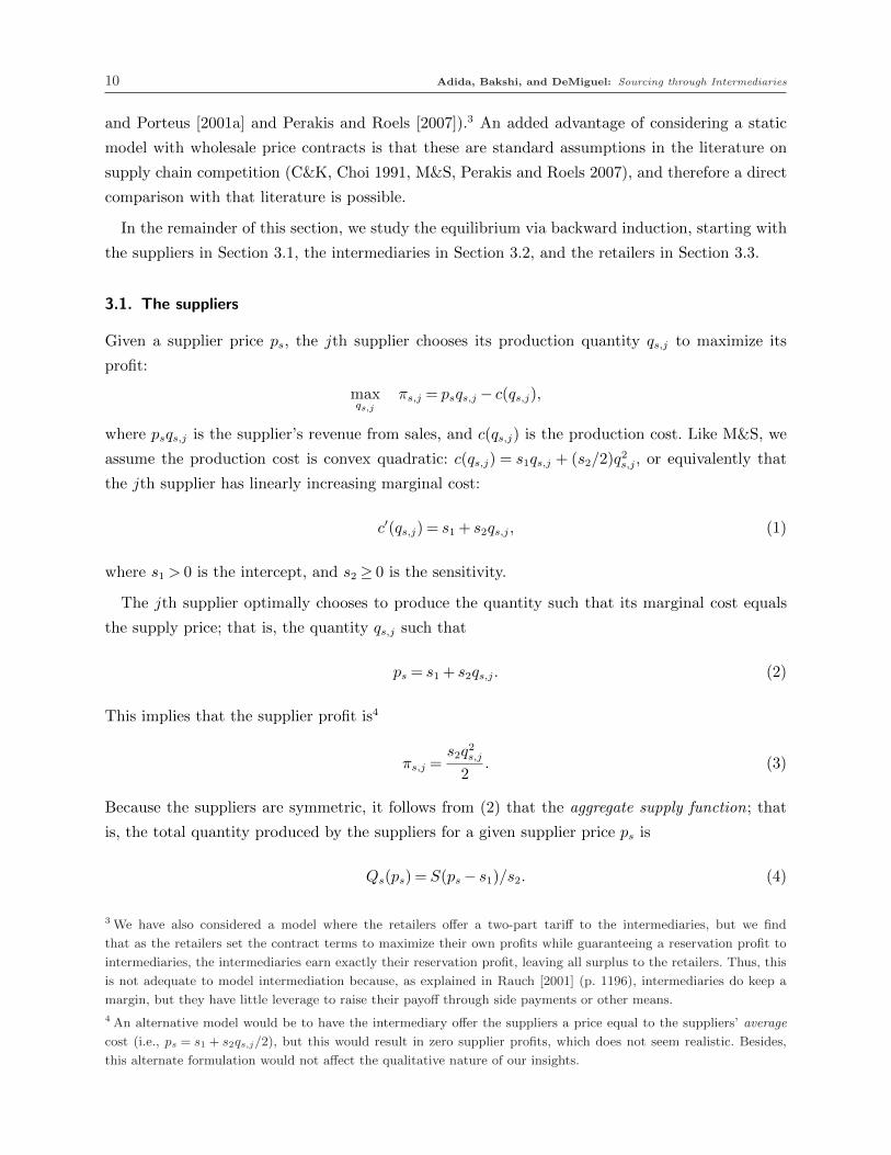
3.1. The suppliers
Given a supplier price ps, the jth supplier chooses its production quantity qs,j to maximize its
profit:
maxqs,j
πs,j = psqs,j − c(qs,j),
where psqs,j is the supplier’s revenue from sales, and c(qs,j) is the production cost. Like M&S, we
assume the production cost is convex quadratic: c(qs,j) = s1qs,j + (s2/2)q2s,j, or equivalently that
the jth supplier has linearly increasing marginal cost:
c′(qs,j) = s1 + s2qs,j, (1)
where s1 > 0 is the intercept, and s2 ≥ 0 is the sensitivity.
The jth supplier optimally chooses to produce the quantity such that its marginal cost equals
the supply price; that is, the quantity qs,j such that
ps = s1 + s2qs,j. (2)
This implies that the supplier profit is4
πs,j =s2q
2s,j
2. (3)
Because the suppliers are symmetric, it follows from (2) that the aggregate supply function; that
is, the total quantity produced by the suppliers for a given supplier price ps is
Qs(ps) = S(ps − s1)/s2. (4)
3 We have also considered a model where the retailers offer a two-part tariff to the intermediaries, but we find
that as the retailers set the contract terms to maximize their own profits while guaranteeing a reservation profit to
intermediaries, the intermediaries earn exactly their reservation profit, leaving all surplus to the retailers. Thus, this
is not adequate to model intermediation because, as explained in Rauch [2001] (p. 1196), intermediaries do keep a
margin, but they have little leverage to raise their payoff through side payments or other means.
4 An alternative model would be to have the intermediary offer the suppliers a price equal to the suppliers’ average
cost (i.e., ps = s1 + s2qs,j/2), but this would result in zero supplier profits, which does not seem realistic. Besides,
this alternate formulation would not affect the qualitative nature of our insights.
Adida, Bakshi, and DeMiguel: Sourcing through Intermediaries 11
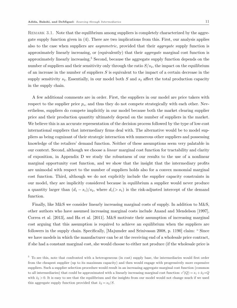
Remark 3.1. Note that the equilibrium among suppliers is completely characterized by the aggre-
gate supply function given in (4). There are two implications from this. First, our analysis applies
also to the case when suppliers are asymmetric, provided that their aggregate supply function is
approximately linearly increasing, or (equivalently) that their aggregate marginal cost function is
approximately linearly increasing.5 Second, because the aggregate supply function depends on the
number of suppliers and their sensitivity only through the ratio S/s2, the impact on the equilibrium
of an increase in the number of suppliers S is equivalent to the impact of a certain decrease in the
supply sensitivity s2. Essentially, in our model both S and s2 affect the total production capacity
in the supply chain.
A few additional comments are in order. First, the suppliers in our model are price takers with
respect to the supplier price ps, and thus they do not compete strategically with each other. Nev-
ertheless, suppliers do compete implicitly in our model because both the market clearing supplier
price and their production quantity ultimately depend on the number of suppliers in the market.
We believe this is an accurate representation of the decision process followed by the type of low-cost
international suppliers that intermediary firms deal with. The alternative would be to model sup-
pliers as being cognizant of their strategic interaction with numerous other suppliers and possessing
knowledge of the retailers’ demand function. Neither of these assumptions seem very palatable in
our context. Second, although we choose a linear marginal cost function for tractability and clarity
of exposition, in Appendix D we study the robustness of our results to the use of a nonlinear
marginal opportunity cost function, and we show that the insight that the intermediary profits
are unimodal with respect to the number of suppliers holds also for a convex monomial marginal
cost function. Third, although we do not explicitly include the supplier capacity constraints in
our model, they are implicitly considered because in equilibrium a supplier would never produce
a quantity larger than (d1 − s1)/s2, where d1(> s1) is the risk-adjusted intercept of the demand
function.
Finally, like M&S we consider linearly increasing marginal costs of supply. In addition to M&S,
other authors who have assumed increasing marginal costs include Anand and Mendelson [1997],
Correa et al. [2013], and Ha et al. [2011]. M&S motivate their assumption of increasing marginal
cost arguing that this assumption is required to achieve an equilibrium when the suppliers are
followers in the supply chain. Specifically, [Majumder and Srinivasan 2008, p. 1190] claim: “ Since
we have models in which the manufacturer can be at the receiving end of a wholesale price contract,
if she had a constant marginal cost, she would choose to either not produce (if the wholesale price is
5 To see this, note that confronted with a heterogeneous (in cost) supply base, the intermediaries would first order
from the cheapest supplier (up to its maximum capacity) and then would engage with progressively more expensive
suppliers. Such a supplier selection procedure would result in an increasing aggregate marginal cost function (common
to all intermediaries) that could be approximated with a linearly increasing marginal cost function: c′(Q) = s1+ s2 ∗Qwith s2 > 0. It is easy to see that the equilibrium and the insights from our model would not change much if we used
this aggregate supply function provided that s2 = s2/S.
12 Adida, Bakshi, and DeMiguel: Sourcing through Intermediaries
lower than his marginal cost), produce an arbitrarily large quantity (if the wholesale price is higher)
or produce an indeterminate quantity (if they are equal).” In addition, we believe this is the most
realistic assumption in the context of intermediary firms that use the existing production capacity
of their network of suppliers to satisfy incidental demand from retailers. Because the suppliers use
existing capacity, they do not make any additional capacity investments and thus they do not incur
any additional fixed costs. One of the key rationales for modeling decreasing marginal cost of supply
(economies of scale) is that any fixed cost of capacity investment can be defrayed over multiple
units. In the absence of incremental fixed costs, it is sufficient for the purposes of decision making
to capture the variable costs. In this setting, although marginal variable costs could be constant
for small quantities, they will inevitably increase as the order quantities approach the capacity
constraint of the suppliers.6 In addition, linearly increasing marginal costs can also be motivated by
relaxing the assumption that suppliers are symmetric, and adopting an asymmetric aggregate view
instead. As discussed in Remark 3.1 and Footnote 5, this would result in an increasing aggregate
marginal cost function (common to all intermediaries) that could be approximated with a linear
function.
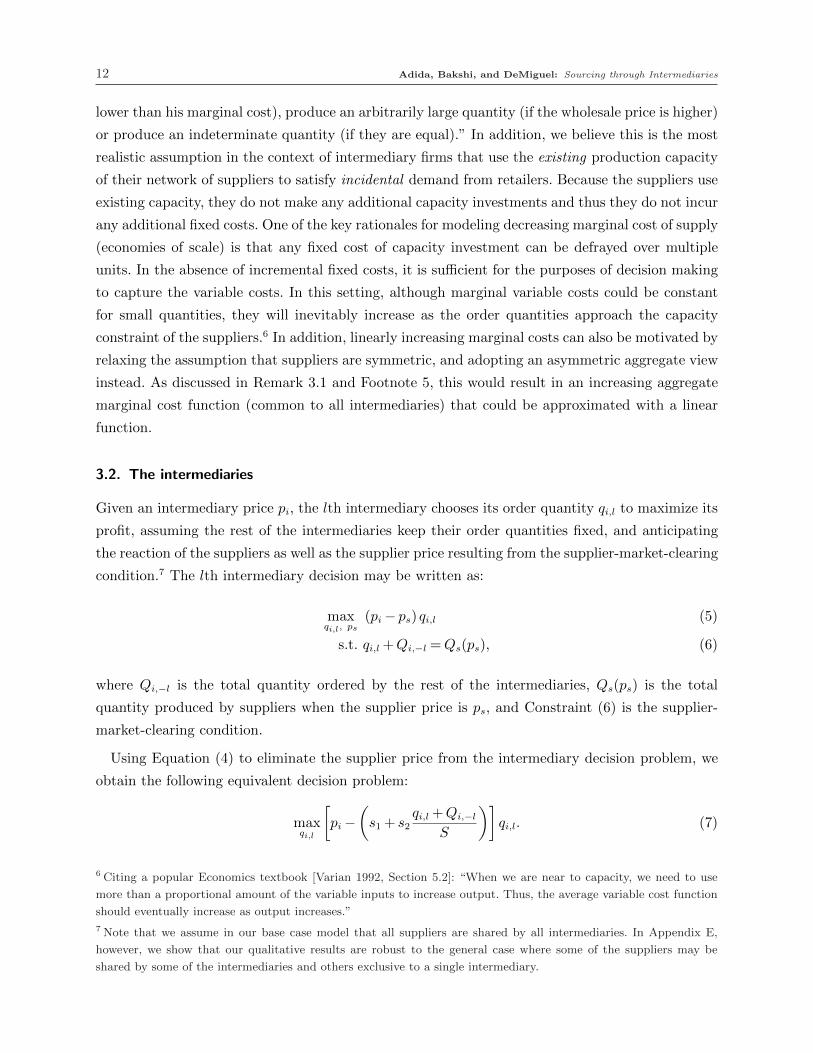
3.2. The intermediaries
Given an intermediary price pi, the lth intermediary chooses its order quantity qi,l to maximize its
profit, assuming the rest of the intermediaries keep their order quantities fixed, and anticipating
the reaction of the suppliers as well as the supplier price resulting from the supplier-market-clearing
condition.7 The lth intermediary decision may be written as:
maxqi,l, ps
(pi − ps) qi,l (5)
s.t. qi,l +Qi,−l =Qs(ps), (6)
where Qi,−l is the total quantity ordered by the rest of the intermediaries, Qs(ps) is the total
quantity produced by suppliers when the supplier price is ps, and Constraint (6) is the supplier-
market-clearing condition.
Using Equation (4) to eliminate the supplier price from the intermediary decision problem, we
obtain the following equivalent decision problem:
maxqi,l
[pi −
(s1 + s2
qi,l +Qi,−l
S
)]qi,l. (7)
6 Citing a popular Economics textbook [Varian 1992, Section 5.2]: “When we are near to capacity, we need to use
more than a proportional amount of the variable inputs to increase output. Thus, the average variable cost function
should eventually increase as output increases.”
7 Note that we assume in our base case model that all suppliers are shared by all intermediaries. In Appendix E,
however, we show that our qualitative results are robust to the general case where some of the suppliers may be
shared by some of the intermediaries and others exclusive to a single intermediary.

Adida, Bakshi, and DeMiguel: Sourcing through Intermediaries 13
Finally, we show in Appendix A that for a given intermediary price pi, the total quantity produced
by intermediaries at equilibrium is
Qi(pi) =SI(pi − s1)
s2(I +1). (8)
3.3. The retailers
To simplify the exposition, we model demand with a deterministic demand function, although we
show in Appendix G that our results generally hold also for the case with a stochastic demand
function. Concretely, we model demand with the following linear inverse demand function8:
pr = d1 − d2Q, (9)
where d1 is the demand intercept and d2 is the demand sensitivity.
The kth retailer profit is
πr,k = (pr − pi)qr,k = (d1 − d2(qr,k +Qr,−k)− pi)qr,k,
where qr,k is the order quantity selected by the kth retailer and Qr,−k is the total quantity ordered
by all other retailers.
Then the kth retailer chooses its order quantity qr,k to maximize its profit, assuming the rest of
the retailers keep their order quantities fixed, and anticipating the intermediary reaction and the
intermediary-market-clearing price pi:
maxqr,k, pi
[d1 − d2(qr,k +Qr,−k)− pi] qr,k (10)
s.t. qr,k +Qr,−k =Qi(pi), (11)
where Qr,−k is the total quantity ordered by the rest of retailers, Qi(pi) is the intermediary equi-
librium quantity for a price pi, and Constraint (11) is the intermediary-market-clearing condition.
Finally, using (8), one can eliminate the intermediary price from the problem and obtain the
following equivalent retailer decision problem:
maxqr,k
[d1 − d2(qr,k +Qr,−k)−
(s1 + s2
I +1
SI(qr,k +Qr,−k)
)]qr,k.
8 Linear demand models have been widely used both in the Economics literature (see, for instance, Singh and Vives
[1984] and Hackner [2003]) as well as in the Operations Management literature (Farahat and Perakis [2011], and
Farahat and Perakis [2009]). C&K assume a deterministic linear inverse demand function. Other authors have also
used it in the context of supply chain competition. Cachon and Lariviere [2005], for instance, mention that the
results for their model with competing retailers can be applied for the particular case of “Cournot competition with
deterministic linear demand”, and they give as an example a deterministic linear inverse demand function for a single
homogeneous product with retailer differentiation.
14 Adida, Bakshi, and DeMiguel: Sourcing through Intermediaries
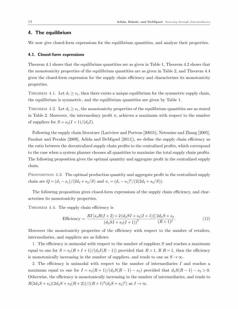
4. The equilibrium
We now give closed-form expressions for the equilibrium quantities, and analyze their properties.
4.1. Closed-form expressions
Theorem 4.1 shows that the equilibrium quantities are as given in Table 1, Theorem 4.2 shows that
the monotonicity properties of the equilibrium quantities are as given in Table 2, and Theorem 4.4
gives the closed-form expression for the supply chain efficiency and characterizes its monotonicity
properties.
Theorem 4.1. Let d1 ≥ s1, then there exists a unique equilibrium for the symmetric supply chain,
the equilibrium is symmetric, and the equilibrium quantities are given by Table 1.
Theorem 4.2. Let d1 ≥ s1, the monotonicity properties of the equilibrium quantities are as stated
in Table 2. Moreover, the intermediary profit πi achieves a maximum with respect to the number
of suppliers for S = s2(I +1)/(d2I).
Following the supply chain literature (Lariviere and Porteus [2001b], Netessine and Zhang [2005],
Farahat and Perakis [2009], Adida and DeMiguel [2011]), we define the supply chain efficiency as
the ratio between the decentralized supply chain profits to the centralized profits, which correspond
to the case when a system planner chooses all quantities to maximize the total supply chain profits.
The following proposition gives the optimal quantity and aggregate profit in the centralized supply
chain.
Proposition 4.3. The optimal production quantity and aggregate profit in the centralized supply
chain are Q= (d1 − s1)/(2d2 + s2/S) and πc = (d1 − s1)2/(2(2d2 + s2/S)).
The following proposition gives closed-form expressions of the supply chain efficiency, and char-
acterizes its monotonicity properties.
Theorem 4.4. The supply chain efficiency is
Efficiency =RI [s2R(I +2)+2(d2SI + s2(I +1))]
(d2SI + s2(I +1))2
2d2S+ s2(R+1)2
. (12)
Moreover the monotonicity properties of the efficiency with respect to the number of retailers,
intermediaries, and suppliers are as follows:
1. The efficiency is unimodal with respect to the number of suppliers S and reaches a maximum
equal to one for S = s2(R+ I +1)/(d2I(R− 1)) provided that R> 1. If R= 1, then the efficiency
is monotonically increasing in the number of suppliers, and tends to one as S →∞.
2. The efficiency is unimodal with respect to the number of intermediaries I and reaches a
maximum equal to one for I = s2(R + 1)/(d2S(R − 1) − s2) provided that d2S(R − 1) − s2 > 0.
Otherwise, the efficiency is monotonically increasing in the number of intermediaries, and tends to
R(2d2S+ s2)(2d2S+ s2(R+2))/((R+1)2(d2S+ s2)2) as I →∞.
Adida, Bakshi, and DeMiguel: Sourcing through Intermediaries 15
3. The efficiency is unimodal with respect to the number of retailers R and reaches a maximum9
equal to one for R = (d2SI + s2(I + 1))/(d2SI − s2) provided that d2SI − s2 > 0. Otherwise, the
efficiency is monotonically increasing in the number of retailers, and tends to s2I(I + 2)(2d2S +
s2)/(d2SI + s2(I +1))2 as R→∞.
4.2. Discussion
Table 2 summarizes the monotonicity properties of the equilibrium quantities. The table gives
several intuitive results: (i) the total quantity produced in the supply chain is increasing in the
number of retailers, intermediaries, and suppliers, and decreasing in the demand and supply sen-
sitivities, (ii) the prices at each tier are decreasing in the number of players in following tiers,
increasing in the number of players in leading tiers, increasing in the supply function sensitivity,
and decreasing in the demand function sensitivity, and (iv) the retailer profit is increasing in the
number of intermediaries and suppliers, but decreasing in the number of retailers, and decreasing
in both the supply and demand sensitivities.
4.2.1. Intermediary profits. Compared to the above findings, the results about the interme-
diary profits are arguably more interesting. Although expectedly the intermediary margin decreases
in the number of intermediaries and increases in the number of retailers, surprisingly the inter-
mediary margin decreases in the number of suppliers. Moreover, since the overall order quantity
is monotonically increasing in the number of suppliers, therefore the intermediary profits are uni-
modal with respect to the number of suppliers, reaching their maximum for a finite number of
suppliers. Based on the results in C&K and Choi [1991], one might have expected that the larger
the supplier base, the larger the market power of the intermediaries and thus the larger their mar-
gin and profits. However, in a world where retailers lead, when the supplier base is “large enough”,
we show that the weakness of the suppliers becomes the weakness of the intermediaries, and the
retailers exploit their leadership position to increase their market power and retain greater supply
chain profits. Specifically, in the presence of an infinite number of suppliers, the retailers know
that the intermediaries can get an unlimited quantity of the product at a price of s1 per unit.
As a result, the retailers can exploit their leader advantage to drive the intermediary price to the
suppliers’ marginal cost s1. In this limiting case, the retailers have all the market power and keep
all profits.
A crucial implication of this result is that intermediaries in global supply chains prefer products
for which the supplier base (existing production capacity) is neither too narrow nor too broad,
because (ceteris paribus) products for which there is an intermediate production capacity available
generate larger intermediary profits. The result also offers some insight into how the financial
9 Note that the values of R,S and I respectively that maximize the efficiency may not be integers, in which case the
maximum would be reached at the integer value just below or above it. To keep the exposition simple, we approximate
the true integer maximum with the possibly non integer expressions above.
16 Adida, Bakshi, and DeMiguel: Sourcing through Intermediaries
performance of trading companies, and consequently of economies reliant on this sector, depends on
the available production capacity. This capacity is a function of various economic and environmental
factors. For instance, Barrie [2013] reports a shortfall in available capacity for 2013 in the fashion
apparel sector, whereas Zhao [2013] points to endemic overcapacity in the Chinese fashion industry
during 1980s and 1990s. Our analysis shows that intermediary profits will be squeezed in either of
these two eventualities; that is, in case of shortfall or excess in available capacity.
4.2.2. Efficiency. Theorem 4.4 gives the closed-form expression for the supply chain efficiency
and characterizes its monotonicity properties. Our main observation is that a supply chain effi-
ciency equal to one (that is, an efficient supply chain) can always be achieved in the presence of
intermediaries provided there is the right balance of competition at the three tiers. To see this,
note from Point 1 in Theorem 4.4 that provided the number of retailers is greater than one, we can
always adjust the number of suppliers so that efficiency one is achieved. Also, note that provided
that there is a sufficiently large number of suppliers and retailers, the condition d2S(R−1)−s2 > 0
will be satisfied, and thus from Point 2 we have that there exists a number of intermediaries for
which the supply chain efficiency is equal to one. Finally, from Point 3 we see that provided there
is a sufficiently large number of suppliers and intermediaries we can always satisfy the condition
d2SI − s2 > 0 and thus there will exist a number of retailers for which the efficiency of the supply
chain is equal to one.
The main takeaway from this analysis is that the presence of an additional tier of intermediaries
in the supply chain does not necessarily introduce an element of inefficiency to the supply chain;
that is, the aggregate supply chain profit in the decentralized chain with intermediaries is not nec-
essarily smaller than that in the centralized (integrated) supply chain. The classic result on double
marginalization would have suggested otherwise (Spengler 1950). However, accounting for competi-
tion in our model is the differentiating feature. It is well known that the relative bargaining strength
of players in a vertical relationship significantly determines the extent of double marginalization.
Further, increasing the number of within-tier competitors reduces a specific player’s bargaining
power in the vertical interaction. Such adjustments to competitive intensity may be carried out at
each tier. We find that there always exists an appropriate balance between horizontal and vertical
competition that completely offsets the effect of double marginalization, and leads to supply chain
efficiency. An implication of this result is that regulators may try and improve the efficiency of
global supply chains by taking measures to encourage a healthy level of competition at each of the
three tiers.
We find, however, that if regulatory intervention is to succeed at improving the overall supply
chain efficiency, it must be carefully tailored to the structure of the supply chain in question. To see
this, note that Proposition 4.2 shows that intermediaries would choose a number of suppliers S =
s2(I+1)/(d2I) in order to maximize their profit. Part 1 of Theorem 4.4, on the other hand, shows
that overall efficiency is maximized for a different number of suppliers S = s2(R+ I+1)/(d2I(R−
Adida, Bakshi, and DeMiguel: Sourcing through Intermediaries 17
1)). For R= 2, the number of suppliers that maximizes the overall supply-chain efficiency is larger
than the number that maximizes intermediary profits. Also, the number of suppliers that maximizes
efficiency is monotonically decreasing in R. This suggests that with high concentration in the retail
tier (small R), a decentralized supply chain is likely to yield a smaller-than-efficient size of the
supply base, and thus subsidizing the intermediaries to enlarge their supply base is likely to improve
the overall efficiency. However, for supply chains with low retailer concentration (large R), such
subsidies are unlikely to help.
Interestingly, Rauch [2001] cites the trade-creating impact of immigrants, expatriates, and foreign
direct investment, as evidence to suggest that intermediaries may not be adequately connecting
buyers and sellers internationally, and thereby makes a case for regulatory intervention to encour-
age a larger supply base. However, Rauch [2001] also points to contradictory evidence: while the
governments of Japan, Korea and Turkey improved trade by encouraging intermediaries to main-
tain larger supply bases through subsidies, similar attempts were unsuccessful in Taiwan and the
U.S. Our analysis above offers a possible explanation for this in terms of retailer tier concentration.
Specifically, we find that regulatory intervention will be effective only if it is tailored to the specific
characteristics of the supply chains.
5. The case with asymmetric information
An important insight from our analysis is that in a supply chain where retailers lead, they take
advantage of their leading position to increase their market power with respect to the interme-
diaries. This leads one to wonder whether intermediaries can exploit their private information to
extract greater rents. For instance, although intermediaries help the retailers overcome some of
their information barriers (e.g., by identifying appropriate suppliers), they may also find it advan-
tageous to withhold certain information from the retailers such as the supply sensitivity. As noted
in the literature on asymmetric information, truthful information sharing must be incentivized: an
agent with private information may choose not to disclose it if beneficial. To answer this question,
in this section we study how the presence of asymmetric information about the supply sensitivity
alters the balance of market power between the retailers and the intermediaries.
5.1. The model and equilibrium
To model asymmetric information, we assume that intermediaries know whether the supply sensi-
tivity is high s2 = sH2 or low s2 = sL2 , but the retailers share the prior belief that there is a probability
ν that the sensitivity is low (s2 = sL2 ) and 1− ν that it is high (s2 = sH2 ).
The kth retailer chooses its order quantity to maximize its expected profit assuming the rest of
the retailers keep their order quantities fixed, and anticipating the reaction of the intermediaries
18 Adida, Bakshi, and DeMiguel: Sourcing through Intermediaries
as well as the intermediary-market-clearing price for each scenario (with low or high sensitivity).10
The kth retailer’s expected profit is:
E[πr,k
]= ν
(d1 − d2(qr,k +Qr,−k)− pLi
)qr,k +(1− ν)
(d1 − d2(qr,k +Qr,−k)− pHi
)qr,k, (13)
where the first (second) term on the right-hand side of (13) corresponds to the profit for the case
with low (high) sensitivity, and the intermediary market clearing prices for the scenarios with low
and high sensitivity, pLi and pHi , are given by Theorem 4.1 as in the case with complete information;
that is, pLi = s1 +(sL2 /S)((I +1)/I)(qr,k +Qr,−k) and pHi = s1 +(sH2 /S)((I +1)/I)(qr,k +Qr,−k).
The following proposition gives closed-form expressions for the expected equilibrium quantities,
where the expectation is taken over the prior distribution, as well as for the realized equilibrium
quantities corresponding to each of the two scenarios with low and high sensitivity.
Proposition 5.1. Let d1 ≥ s1, then there exists a unique equilibrium for the supply chain with
asymmetric information and the equilibrium is symmetric. Moreover:
1. The aggregate quantity ordered by the retailers is
Q=RSI
(d2SI + s2(I +1))
d1 − s1(R+1)
, (14)
where s2 is the expected supply sensitivity; that is, s2 = νsL2 +(1− ν)sH2 .
2. The realized equilibrium quantities for the scenario with low (high) sensitivity are given by the
last column of Table 1 after replacing Q with the aggregate quantity given by (14), and the supply
sensitivity s2 with the sensitivity corresponding to the scenario with low sL2 (high sH2 ) sensitivity.
3. The expected equilibrium quantities are given by the same expressions as for the case with
perfect information (that is, by the third column of Table 1) after replacing the supply sensitivity
s2 by the expected supply sensitivity s2.
5.2. The impact of asymmetric information
We characterize the impact of asymmetric information on both the expected and the realized equi-
librium quantities.11 The impact of asymmetric information on the expected equilibrium quantities
is important from the perspective of the retailer. Specifically, the impact of asymmetric information
on the expected retailer profits is the value of perfect information. If the value of information is
large, then the retailers have an incentive to gather further information about the supply sensitivity.
10 This is the equivalent of a pooling contract in the standard treatment of games with asymmetric information.
Screening of the different types of intermediary is not possible in the context of wholesale price contracts because
only one contracting variable (price) is available. Note that we restrict our analysis to wholesale price contracts for
the reasons argued in Section 3.
11 For expected equilibrium quantities, we compare the expected equilibrium quantities for the case with asymmetric
information (given by Part 3 of Proposition 5.1), with the expected equilibrium quantities for the case with perfect
information (computed by taking expectations over the prior distribution of the perfect information equilibrium
quantities corresponding to the scenarios with low and high sensitivity).
Adida, Bakshi, and DeMiguel: Sourcing through Intermediaries 19
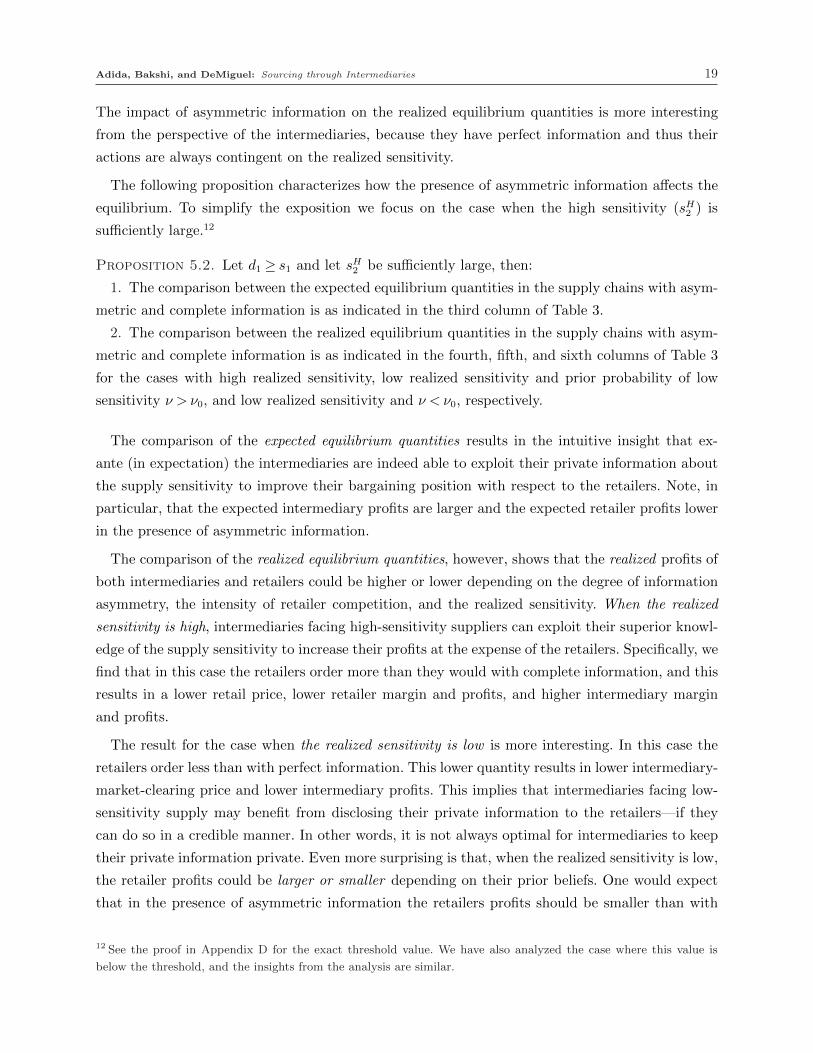
The impact of asymmetric information on the realized equilibrium quantities is more interesting
from the perspective of the intermediaries, because they have perfect information and thus their
actions are always contingent on the realized sensitivity.
The following proposition characterizes how the presence of asymmetric information affects the
equilibrium. To simplify the exposition we focus on the case when the high sensitivity (sH2 ) is
sufficiently large.12
Proposition 5.2. Let d1 ≥ s1 and let sH2 be sufficiently large, then:
1. The comparison between the expected equilibrium quantities in the supply chains with asym-
metric and complete information is as indicated in the third column of Table 3.
2. The comparison between the realized equilibrium quantities in the supply chains with asym-
metric and complete information is as indicated in the fourth, fifth, and sixth columns of Table 3
for the cases with high realized sensitivity, low realized sensitivity and prior probability of low
sensitivity ν > ν0, and low realized sensitivity and ν < ν0, respectively.
The comparison of the expected equilibrium quantities results in the intuitive insight that ex-
ante (in expectation) the intermediaries are indeed able to exploit their private information about
the supply sensitivity to improve their bargaining position with respect to the retailers. Note, in
particular, that the expected intermediary profits are larger and the expected retailer profits lower
in the presence of asymmetric information.
The comparison of the realized equilibrium quantities, however, shows that the realized profits of
both intermediaries and retailers could be higher or lower depending on the degree of information
asymmetry, the intensity of retailer competition, and the realized sensitivity. When the realized
sensitivity is high, intermediaries facing high-sensitivity suppliers can exploit their superior knowl-
edge of the supply sensitivity to increase their profits at the expense of the retailers. Specifically, we
find that in this case the retailers order more than they would with complete information, and this
results in a lower retail price, lower retailer margin and profits, and higher intermediary margin
and profits.
The result for the case when the realized sensitivity is low is more interesting. In this case the
retailers order less than with perfect information. This lower quantity results in lower intermediary-
market-clearing price and lower intermediary profits. This implies that intermediaries facing low-
sensitivity supply may benefit from disclosing their private information to the retailers—if they
can do so in a credible manner. In other words, it is not always optimal for intermediaries to keep
their private information private. Even more surprising is that, when the realized sensitivity is low,
the retailer profits could be larger or smaller depending on their prior beliefs. One would expect
that in the presence of asymmetric information the retailers profits should be smaller than with
12 See the proof in Appendix D for the exact threshold value. We have also analyzed the case where this value is
below the threshold, and the insights from the analysis are similar.

20 Adida, Bakshi, and DeMiguel: Sourcing through Intermediaries
perfect information, but Table 3 shows that, when the realized sensitivity is low, the retailer profit
is lower if and only its prior probability of low sensitivity (ν) is lower than a certain threshold (ν0):
ν < ν0 ≡ (I +1)(sH2 −RsL2 )− d2SI(R− 1)
(I +1)(sH2 − sL2 ).
For the case with a single retailer we have that ν0 = 1, and thus monopolist retailer profits are
always lower in the case with asymmetric information. Indeed, a monopolist retailer with perfect
information on supply sensitivity must be able to extract larger profits from the supply chain than
in the absence of perfect information, regardless of whether the realized supply sensitivity is low
or high.
A more interesting result occurs when there are several competing retailers. For this case, when
the retailers’ prior probability of low sensitivity is small (ν < ν0), the retailer profits are smaller
than in the case with complete information. When the retailers’ prior probability of low sensitivity
is moderate (ν > ν0), however, their profits are larger in the presence of asymmetric information.
The explanation for this is that in the case with multiple competing retailers, the presence of
asymmetric information has a negative and a positive effect on retailer profits. The negative effect
is that the retailers lack information about the supply sensitivity that would help to identify the
optimal quantity to select. The positive effect, however, is that this missing information attenuates
the intensity of competition among retailers because the retailers’ prior belief is that the supply
sensitivity is on average higher than it actually is and thus they choose a lower quantity, which
results in lower intermediary-market-clearing price. For the case where the prior probability of
low sensitivity is low, the negative effect (incomplete information) dominates; for the case where
the prior probability of low sensitivity is moderate, the positive effect of asymmetric information
(competition mitigation) dominates. This result is illustrated in Figure 2.
Finally, the following proposition shows that, although the insight that intermediary profits are
unimodal with respect to the number of suppliers is robust to the presence of asymmetric infor-
mation, the number of suppliers that maximizes intermediary profits in the case with asymmetric
information is larger (smaller) than in the case with complete information depending on whether
the realized sensitivity is low (high).
Proposition 5.3. Let d1 ≥ s1, then the intermediary profits in the presence of asymmetric infor-
mation are unimodal with respect to the number of suppliers, and the number of suppliers that
maximizes intermediary profits is larger (smaller) in the presence of asymmetric information for
the case with s2 = sL2 (s2 = sH2 ).
The main insight from Proposition 5.3 is that the presence of asymmetric information can result
in alterations to the intermediaries’ preferred product portfolio. When the realized sensitivity is
low (high), the preferred product portfolio is biased towards products with more (less) available
production capacity.
Adida, Bakshi, and DeMiguel: Sourcing through Intermediaries 21
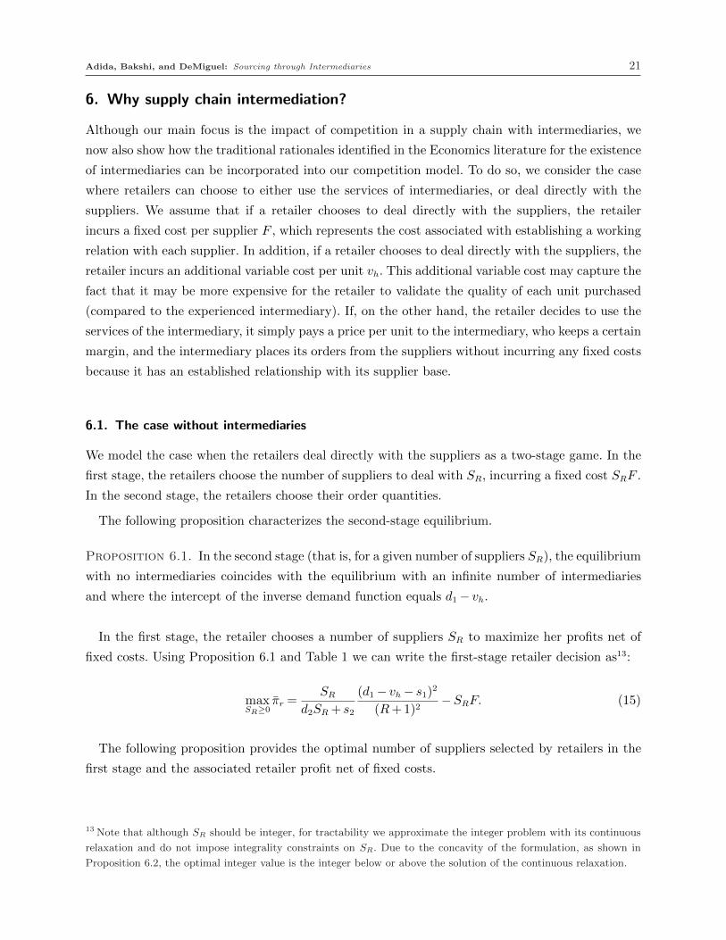
6. Why supply chain intermediation?
Although our main focus is the impact of competition in a supply chain with intermediaries, we
now also show how the traditional rationales identified in the Economics literature for the existence
of intermediaries can be incorporated into our competition model. To do so, we consider the case
where retailers can choose to either use the services of intermediaries, or deal directly with the
suppliers. We assume that if a retailer chooses to deal directly with the suppliers, the retailer
incurs a fixed cost per supplier F , which represents the cost associated with establishing a working
relation with each supplier. In addition, if a retailer chooses to deal directly with the suppliers, the
retailer incurs an additional variable cost per unit vh. This additional variable cost may capture the
fact that it may be more expensive for the retailer to validate the quality of each unit purchased
(compared to the experienced intermediary). If, on the other hand, the retailer decides to use the
services of the intermediary, it simply pays a price per unit to the intermediary, who keeps a certain
margin, and the intermediary places its orders from the suppliers without incurring any fixed costs
because it has an established relationship with its supplier base.
6.1. The case without intermediaries
We model the case when the retailers deal directly with the suppliers as a two-stage game. In the
first stage, the retailers choose the number of suppliers to deal with SR, incurring a fixed cost SRF .
In the second stage, the retailers choose their order quantities.
The following proposition characterizes the second-stage equilibrium.
Proposition 6.1. In the second stage (that is, for a given number of suppliers SR), the equilibrium
with no intermediaries coincides with the equilibrium with an infinite number of intermediaries
and where the intercept of the inverse demand function equals d1 − vh.
In the first stage, the retailer chooses a number of suppliers SR to maximize her profits net of
fixed costs. Using Proposition 6.1 and Table 1 we can write the first-stage retailer decision as13:
maxSR≥0
πr =SR
d2SR + s2
(d1 − vh − s1)2
(R+1)2−SRF. (15)
The following proposition provides the optimal number of suppliers selected by retailers in the
first stage and the associated retailer profit net of fixed costs.
13 Note that although SR should be integer, for tractability we approximate the integer problem with its continuous
relaxation and do not impose integrality constraints on SR. Due to the concavity of the formulation, as shown in
Proposition 6.2, the optimal integer value is the integer below or above the solution of the continuous relaxation.
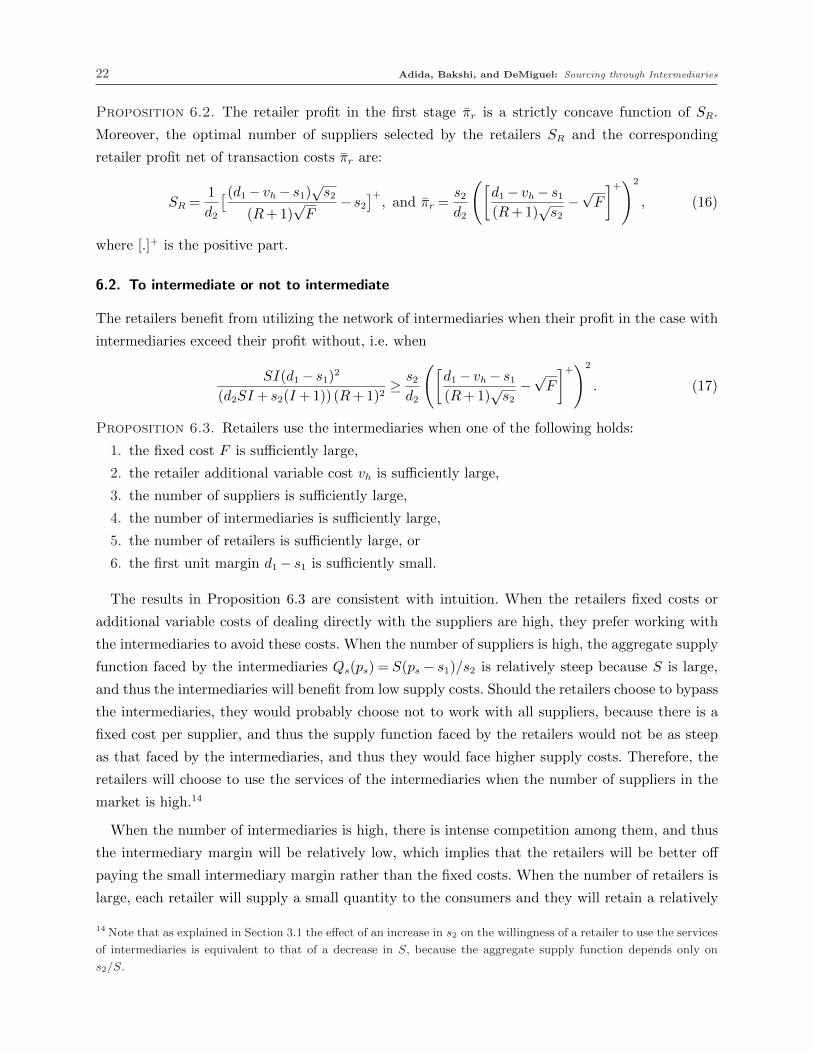
22 Adida, Bakshi, and DeMiguel: Sourcing through Intermediaries
Proposition 6.2. The retailer profit in the first stage πr is a strictly concave function of SR.
Moreover, the optimal number of suppliers selected by the retailers SR and the corresponding
retailer profit net of transaction costs πr are:
SR =1
d2
[(d1 − vh − s1)√s2
(R+1)√F
− s2]+
, and πr =s2d2
([d1 − vh − s1(R+1)
√s2
−√F
]+)2
, (16)
where [.]+ is the positive part.
6.2. To intermediate or not to intermediate
The retailers benefit from utilizing the network of intermediaries when their profit in the case with
intermediaries exceed their profit without, i.e. when
SI(d1 − s1)2
(d2SI + s2(I +1)) (R+1)2≥ s2
d2
([d1 − vh − s1(R+1)
√s2
−√F
]+)2
. (17)
Proposition 6.3. Retailers use the intermediaries when one of the following holds:
1. the fixed cost F is sufficiently large,
2. the retailer additional variable cost vh is sufficiently large,
3. the number of suppliers is sufficiently large,
4. the number of intermediaries is sufficiently large,
5. the number of retailers is sufficiently large, or
6. the first unit margin d1 − s1 is sufficiently small.
The results in Proposition 6.3 are consistent with intuition. When the retailers fixed costs or
additional variable costs of dealing directly with the suppliers are high, they prefer working with
the intermediaries to avoid these costs. When the number of suppliers is high, the aggregate supply
function faced by the intermediaries Qs(ps) = S(ps − s1)/s2 is relatively steep because S is large,
and thus the intermediaries will benefit from low supply costs. Should the retailers choose to bypass
the intermediaries, they would probably choose not to work with all suppliers, because there is a
fixed cost per supplier, and thus the supply function faced by the retailers would not be as steep
as that faced by the intermediaries, and thus they would face higher supply costs. Therefore, the
retailers will choose to use the services of the intermediaries when the number of suppliers in the
market is high.14
When the number of intermediaries is high, there is intense competition among them, and thus
the intermediary margin will be relatively low, which implies that the retailers will be better off
paying the small intermediary margin rather than the fixed costs. When the number of retailers is
large, each retailer will supply a small quantity to the consumers and they will retain a relatively
14 Note that as explained in Section 3.1 the effect of an increase in s2 on the willingness of a retailer to use the services
of intermediaries is equivalent to that of a decrease in S, because the aggregate supply function depends only on
s2/S.
Adida, Bakshi, and DeMiguel: Sourcing through Intermediaries 23
small margin. Under these circumstances, it will most likely not be profitable for the retailers to
pay any fixed costs. Finally, when the first unit margin d1− s1 is small, the retailer margin will be
small (as it must be smaller than the first unit margin), and therefore it may not be profitable to
pay any fixed costs.
6.3. The squeezed middleman
Proposition 6.3 throws some light over the decline in profitability of supply chain intermediaries in
recent years. Some speculate that this may be the result of retailers increasingly sourcing directly
from suppliers; Chu [2012] claims: “children apparel companies such as Carter’s Inc. and Gymboree
Corp. have said they plan to obtain more of their products directly in coming years”. Others,
such as Hughes and Kirk [2013], point at the low margins of supply chain intermediaries due to
increasing labor costs in countries such as China.
Our analysis shows that while increasing manufacturing costs in China may indeed be hurting the
operating profits of intermediaries, that is not likely to be the reason behind the increasing number
of retailers that choose to source directly from the suppliers. Specifically, Part 6 in Proposition 6.3
shows that increasing manufacturing costs, which result in lower margins, can only encourage
retailers to use the services of intermediaries. Therefore the motivation for retailers increasingly
sourcing directly from low-cost suppliers across Asia is likely to be driven by a reduction in the
fixed costs associated with retailers working with low-cost suppliers, or as Hughes and Kirk [2013]
put it: “China is no longer the mystery it was to western buyers a decade ago”.
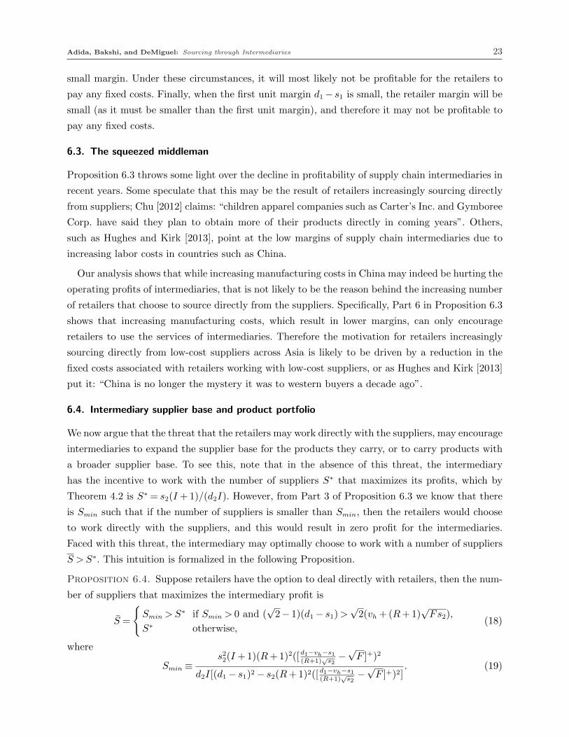
6.4. Intermediary supplier base and product portfolio
We now argue that the threat that the retailers may work directly with the suppliers, may encourage
intermediaries to expand the supplier base for the products they carry, or to carry products with
a broader supplier base. To see this, note that in the absence of this threat, the intermediary
has the incentive to work with the number of suppliers S∗ that maximizes its profits, which by
Theorem 4.2 is S∗ = s2(I +1)/(d2I). However, from Part 3 of Proposition 6.3 we know that there
is Smin such that if the number of suppliers is smaller than Smin, then the retailers would choose
to work directly with the suppliers, and this would result in zero profit for the intermediaries.
Faced with this threat, the intermediary may optimally choose to work with a number of suppliers
S >S∗. This intuition is formalized in the following Proposition.
Proposition 6.4. Suppose retailers have the option to deal directly with retailers, then the num-
ber of suppliers that maximizes the intermediary profit is
S =
{Smin >S∗ if Smin > 0 and (
√2− 1)(d1 − s1)>
√2(vh +(R+1)
√Fs2),
S∗ otherwise,(18)
where
Smin ≡s22(I +1)(R+1)2([d1−vh−s1
(R+1)√s2
−√F ]+)2
d2I[(d1 − s1)2 − s2(R+1)2([d1−vh−s1(R+1)
√s2
−√F ]+)2]
. (19)

24 Adida, Bakshi, and DeMiguel: Sourcing through Intermediaries
Proposition 6.4 implies that, when the condition in (18) holds, the threat that the retailers may
go deal directly with suppliers gives the intermediaries an incentive to either expand their supplier
base for products they are carrying, or carry products with a broader supplier base, in order to
ensure the retailers make use of their services.
Figure 3 shows the intermediary profit as a function of the number of suppliers for two cases
with different fixed cost F . The left panel has a higher fixed cost, and in this case the intermediary
is better off working with S∗ suppliers. The right panel has a lower fixed cost, and this pushes the
intermediary to prefer working with a higher number of suppliers Smin.
7. Conclusion
We study the impact of horizontal and vertical competition on sourcing arrangements that operate
through intermediaries. Our focus on the role of competition distinguishes our work from the bulk of
the prior literature on intermediation, which provides rationales for the existence of intermediaries.
Also, our considering a model with retailers as Stackelberg leaders distinguishes our work from the
prior literature on supply chain competition. Our main result suggests that intermediaries prefer
products for which the supply base is neither too broad nor too narrow. This result not only helps
clarify the characteristics of products which are likely to be favored by intermediaries, but also
helps explain how financial performance of intermediaries, and hence, of economies reliant on this
sector, may vary over time, depending upon the availability of supply.
The intermediary tier in global supply chains has seen a number of acquisitions of late, accompa-
nied with speculation about further acquisitions (Reuters 2012). A natural question then is: What
is the impact of these acquisitions on not only the acquiring firm, but also on the efficiency of
the entire supply chain? Our competition model provides a framework to think about these issues.
Specifically, we find that right balance of horizontal and vertical competition can entirely offset
the adverse effect of double marginalization.
Our analysis provides additional perspective on the puzzle identified by Rauch [2001] that while
the governments of Japan, Korea, and Turkey succeeded in improving trade by subsidizing the
intermediaries to widen their supplier base, similar attempts failed in Taiwan and the U.S. Con-
cretely, our analysis show thats in order for regulatory intervention in a specific tier in the supply
chain to be successful, it must be carefully tailored to the structure of the entire supply chain in
question.
Finally, we study the impact of asymmetric information in the context of supply chain inter-
mediation, and find that when the realized supply sensitivity is low, competing retailers may be
better off at the expense of the intermediaries compared to the case with perfect information. In
fact, intermediaries facing low-sensitivity demand may prefer to reveal their private information
to the retailers if they can do so credibly.
Appendix A: Tables
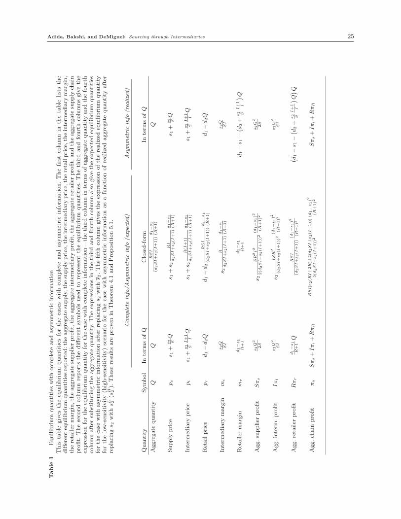
Adida, Bakshi, and DeMiguel: Sourcing through Intermediaries 25
Table
1Equilibrium
quantities
withcomplete
andasymmetricinform
ation
This
table
gives
theequilibrium
quantities
forthecaseswith
complete
and
asymmetricinform
ation.Thefirstcolumn
inthetable
liststhe
differen
tequilibrium
quantities
reported
:theaggregate
supply,thesupply
price,theinterm
ediary
price,theretailprice,theinterm
ediary
margin,
theretailer
margin,theaggregate
supplier
profit,theaggregate
interm
ediary
profit,theaggregate
retailer
profit,andtheaggregate
supply
chain
profit.
Thesecondcolumnreportsthedifferen
tsymbols
usedto
representtheequilibrium
quantities.Thethirdandfourthcolumnsgivethe
expressionfortheequilibrium
quantity
forthecase
withcomplete
inform
ation—
thethirdcolumnin
term
sofaggregate
quantity
andthefourth
columnafter
substitutingtheaggregate
quantity.Theexpressionsin
thethirdandfourthcolumnalsogivetheexpectedequilibrium
quantities
forthecase
withasymmetricinform
ationafter
replacings 2
withs 2.Thefifthcolumngives
theexpressionoftherealizedequilibrium
quantity
forthelow-sen
sitivity(high-sen
sitivity)scen
arioforthecase
withasymmetricinform
ationasafunctionofrealizedaggregate
quantity
after
replacings 2
withsL 2
(sH 2).
Theseresultsare
proven
inTheorem
4.1
andProposition5.1.
Complete
info/Asymmetricinfo
(expected)
Asymmetricinfo
(realized)
Quantity
Symbol
Interm
sofQ
Closed-form
Interm
sofQ
Aggregate
quantity
RSI
(d2SI+s2(I
+1))
d1−s1
(R+1)
Q
Supply
price
ps
s 1+
s2 SQ
s 1+s 2
RI
d2SI+s2(I
+1)d1−s1
(R+1)
s 1+
s2 SQ
Interm
ediary
price
pi
s 1+
s2 S
I+1
IQ
s 1+s 2
R(I
+1)
d2SI+s2(I
+1)d1−s1
(R+1)
s 1+
s2 S
I+1
IQ
Retailprice
pr
d1−d2Q
d1−d2
RSI
(d2SI+s2(I
+1))
d1−s1
(R+1)
d1−d2Q
Interm
ediary
margin
mi
s2Q
SI
s 2R
d2SI+s2(I
+1)d1−s1
(R+1)
s2Q
SI
Retailer
margin
mr
d1−s1
R+1
d1−s1
R+1
d1−s 1
−( d
2+
s2 S
I+1
I
) Q
Agg.supplier
profit
Sπs
s2Q
2
2S
s 2SR
2I2
2(d
2SI+s2(I
+1))
2(d
1−s1)2
(R+1)2
s2Q
2
2S
Agg.interm
.profit
Iπi
s2Q
2
SI
s 2ISR
2
(d2SI+s2(I
+1))
2(d
1−s1)2
(R+1)2
s2Q
2
SI
Agg.retailer
profit
Rπr
d1−s1
R+1Q
RSI
(d2SI+s2(I
+1))
(d1−s1)2
(R+1)2
( d1−s 1
−( d
2+
s2 S
I+1
I
) Q) Q
Agg.chain
profit
πa
Sπs+Iπi+RπR
RSI[s
2(R
I+2R)+
2(d
2SI+s2(I
+1))]
2(d
2SI+s2(I
+1))
2(d
1−s1)2
(R+1)2
Sπs+Iπi+RπR
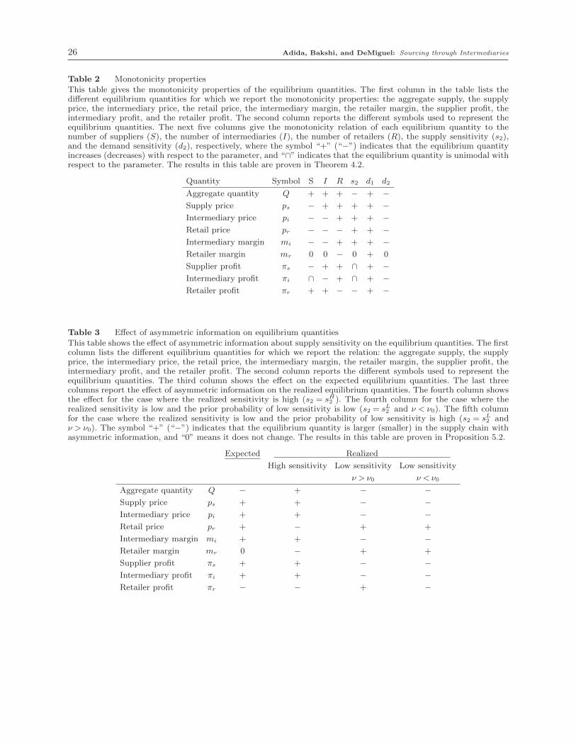
26 Adida, Bakshi, and DeMiguel: Sourcing through Intermediaries
Table 2 Monotonicity properties
This table gives the monotonicity properties of the equilibrium quantities. The first column in the table lists thedifferent equilibrium quantities for which we report the monotonicity properties: the aggregate supply, the supplyprice, the intermediary price, the retail price, the intermediary margin, the retailer margin, the supplier profit, theintermediary profit, and the retailer profit. The second column reports the different symbols used to represent theequilibrium quantities. The next five columns give the monotonicity relation of each equilibrium quantity to thenumber of suppliers (S), the number of intermediaries (I), the number of retailers (R), the supply sensitivity (s2),and the demand sensitivity (d2), respectively, where the symbol “+” (“−”) indicates that the equilibrium quantityincreases (decreases) with respect to the parameter, and “∩” indicates that the equilibrium quantity is unimodal withrespect to the parameter. The results in this table are proven in Theorem 4.2.
Quantity Symbol S I R s2 d1 d2
Aggregate quantity Q + + + − + −Supply price ps − + + + + −Intermediary price pi − − + + + −Retail price pr − − − + + −Intermediary margin mi − − + + + −Retailer margin mr 0 0 − 0 + 0
Supplier profit πs − + + ∩ + −Intermediary profit πi ∩ − + ∩ + −Retailer profit πr + + − − + −
Table 3 Effect of asymmetric information on equilibrium quantities
This table shows the effect of asymmetric information about supply sensitivity on the equilibrium quantities. The firstcolumn lists the different equilibrium quantities for which we report the relation: the aggregate supply, the supplyprice, the intermediary price, the retail price, the intermediary margin, the retailer margin, the supplier profit, theintermediary profit, and the retailer profit. The second column reports the different symbols used to represent theequilibrium quantities. The third column shows the effect on the expected equilibrium quantities. The last threecolumns report the effect of asymmetric information on the realized equilibrium quantities. The fourth column showsthe effect for the case where the realized sensitivity is high (s2 = sH2 ). The fourth column for the case where therealized sensitivity is low and the prior probability of low sensitivity is low (s2 = sL2 and ν < ν0). The fifth columnfor the case where the realized sensitivity is low and the prior probability of low sensitivity is high (s2 = sL2 andν > ν0). The symbol “+” (“−”) indicates that the equilibrium quantity is larger (smaller) in the supply chain withasymmetric information, and “0” means it does not change. The results in this table are proven in Proposition 5.2.
Expected Realized
High sensitivity Low sensitivity Low sensitivity
ν > ν0 ν < ν0
Aggregate quantity Q − + − −Supply price ps + + − −Intermediary price pi + + − −Retail price pr + − + +
Intermediary margin mi + + − −Retailer margin mr 0 − + +
Supplier profit πs + + − −Intermediary profit πi + + − −Retailer profit πr − − + −
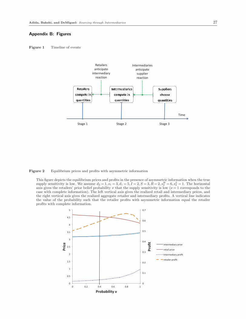
Adida, Bakshi, and DeMiguel: Sourcing through Intermediaries 27
Appendix B: Figures
Figure 1 Timeline of events
�������������� �� ���������
������������������ �� ���������
������������� ���������
�Retailers
anticipate
intermediary
reaction
Intermediaries
anticipate
supplier
reaction
Time
Stage 1 Stage 2 Stage 3
Figure 2 Equilibrium prices and profits with asymmetric information
This figure depicts the equilibrium prices and profits in the presence of asymmetric information when the truesupply sensitivity is low. We assume d2 = 1, s1 = 3, d1 = 5, I = 2, S = 3,R= 2, sH2 = 6, sL2 = 1. The horizontalaxis gives the retailers’ prior belief probability ν that the supply sensitivity is low (ν = 1 corresponds to thecase with complete information). The left vertical axis gives the realized retail and intermediary prices, andthe right vertical axis gives the realized aggregate retailer and intermediary profits. A vertical line indicatesthe value of the probability such that the retailer profits with asymmetric information equal the retailerprofits with complete information.
!"
!#$"
!#%"
!#&"
!#'"
!#("
!#)"
!#*"
!"
!#("
$"
$#("
%"
%#("
&"
&#("
'"
'#("
("
!" !#%" !#'" !#)" !#+" $"
!"#$%&
!"'()&
!"#*+*','%-&.&
,-./01/2,304"50,6/"
0/.3,7"50,6/"
,-./01/2,304"5089."
0/.3,7/0"5089."
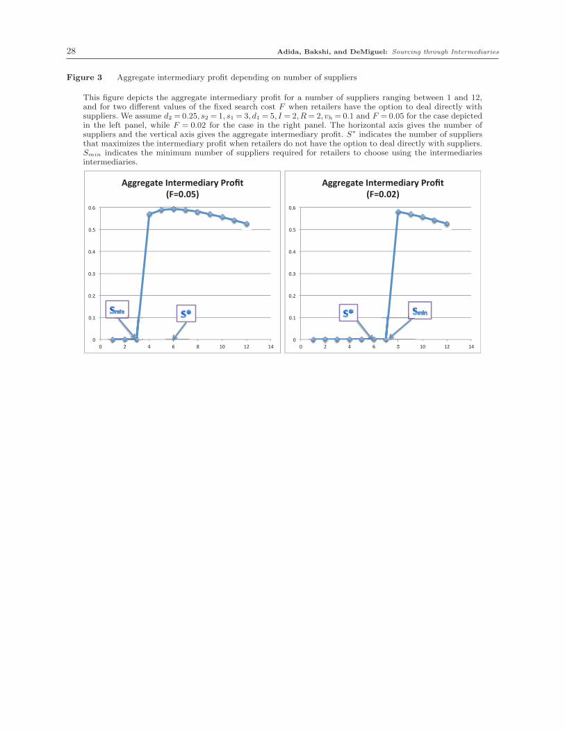
28 Adida, Bakshi, and DeMiguel: Sourcing through Intermediaries
Figure 3 Aggregate intermediary profit depending on number of suppliers
This figure depicts the aggregate intermediary profit for a number of suppliers ranging between 1 and 12,and for two different values of the fixed search cost F when retailers have the option to deal directly withsuppliers. We assume d2 = 0.25, s2 = 1, s1 = 3, d1 = 5, I = 2,R= 2, vh = 0.1 and F = 0.05 for the case depictedin the left panel, while F = 0.02 for the case in the right panel. The horizontal axis gives the number ofsuppliers and the vertical axis gives the aggregate intermediary profit. S∗ indicates the number of suppliersthat maximizes the intermediary profit when retailers do not have the option to deal directly with suppliers.Smin indicates the minimum number of suppliers required for retailers to choose using the intermediariesintermediaries.
!"
!#$"
!#%"
!#&"
!#'"
!#("
!#)"
!" %" '" )" *" $!" $%" $'"
!""#$"%&$'()&$#*$+,%#-'.#/0&'
12345467'
)"%"%"
!"
!#$"
!#%"
!#&"
!#'"
!#("
!#)"
!" %" '" )" *" $!" $%" $'"
!""#$"%&$'()&$#*$+,%#-'.#/0&'
12345467'
)")" *"
Adida, Bakshi, and DeMiguel: Sourcing through Intermediaries 29
References
Adida, E., V. DeMiguel. 2011. Supply chain competition with multiple manufacturers and retailers.
Operations Research 59(1) 156–172.
Anand, K.S., H. Mendelson. 1997. Information and organization for horizontal multimarket coor-
dination. Management Science 43(12) 1609–1627.
Babich, V., Z. Yang. 2014. Should buyers use procurement service providers when suppliers have
private information about supply disruptions? Forthcoming in Management Science.
Barrie, L. 2013. Outlook 2013: Apparel industry challenges. Just-Style.
Belavina, E., K. Girotra. 2012. Global sourcing through intermediaries. Management Science 58(9)
1614–1631.
Bernstein, F., A. Federgruen. 2005. Decentralized supply chains with competing retailers under
demand uncertainty. Management Science 51(1) 18–29.
Biglaiser, G. 1993. Middlemen as experts. The RAND Journal of Economics 24(2) 212–223.
Cachon, G.P., M.A. Lariviere. 2005. Supply chain coordination with revenue-sharing contracts:
strengths and limitations. Management Science 51(1) 30–44.
Carr, S.M., U.S. Karmarkar. 2005. Competition in multi-echelon assembly supply chains. Man-
agement Science 51(1) 45–59.
Cho, S.H. 2013. Horizontal mergers in multi-tier decentralized supply chains. Forthcoming in
Management Science.
Choi, S.C. 1991. Price competition in a channel structure with a common retailer. Marketing
Science 10(4) 271–296.
Christopher, M., R. Lowson, H. Peck. 2004. Creating agile supply chains in the fashion industry.
International Journal of Retail & Distribution Management 32(8) 367–376.
Chu, K. 2012. Big retail squeezes Hong Kong middleman. Wall Street Journal.
Corbett, C.J., U.S. Karmarkar. 2001. Competition and structure in serial supply chains with
deterministic demand. Management Science 47(7) 966–978.
Correa, J.R., N. Figueroa, R. Lederman, N.E. Stier-Moses. 2013. Pricing with markups in industries
with increasing marginal costs. Forthcoming in Mathematical Programming.
Cottle, R.W, J.-S. Pang, R.E. Stone. 2009. The Linear Complementarity Problem. Society for
Industrial and Applied Mathematics, Philadelphia.
Farahat, A., G. Perakis. 2009. Profit loss in differentiated oligopolies. Operations Research Letters
37(1) 43–46.
Farahat, A., G. Perakis. 2011. Technical note—A comparison of Bertrand and Cournot profits in
oligopolies with differentiated products. Operations Research 59(2) 507–513.
Federgruen, A., M. Hu. 2013. Sequential multi-product price competition in supply chain networks.
Rotman School of Management working paper.

30 Adida, Bakshi, and DeMiguel: Sourcing through Intermediaries
Fung, V.K., W.K. Fung, Y. Wind. 2008. Competing in a Flat World: Building Enterprises for a
Borderless World . Wharton School Publishing, Philadelphia.
Ha, A., S. Tong, H. Zhang. 2011. Sharing demand information in competing supply chains with
production diseconomies. Management Science 57(3) 566–581.
Ha-Brookshire, J., B. Dyer. 2008. Apparel import intermediaries the impact of a hyperdynamic
environment on U.S. apparel firms. Clothing and Textiles Research Journal 26(1) 66–90.
Hackner, J. 2003. A note on price and quantity competition in differentiated oligopolies. Journal
of Economic Theory 93(2) 223–239.
Hsing, Y. 1999. Trading companies in Taiwan’s fashion shoe networks. Journal of International
Economics 48(1) 101–120.
Hughes, J., S. Kirk. 2013. Li & Fung: Devotion turns to doubt. Financial Times.
Knowledge@Wharton. 2007. Li and Fung’s Bruce Rockowitz: Managing supply chains
in a ‘flat’ world. http://www.knowledgeatwharton.com.cn/index.cfm?fa=
viewfeature&articleid=1656&languageid=1.
Kopczak, L.R., M.E. Johnson. 2003. The supply-chain management effect. MIT Sloan Management
Review 44(3) 27–34.
Lafontaine, F., M. Slade. 2012. Inter-firm contracts. R. Gibbons, J. Roberts, eds., The Handbook
of Organizational Economics. Princeton University Press, 958–1013.
Lariviere, M.A., E.L. Porteus. 2001a. Selling to the newsvendor: An analysis of price-only contracts.
Manufacturing & Service Operations Management 3(4) 293–305.
Lariviere, M.A., E.L. Porteus. 2001b. Selling to the newsvendor: An analysis of price-only contracts.
Manufacturing & Service Operations Management 3(4) 293–305.
Majumder, P., A. Srinivasan. 2008. Leadership and competition in network supply chains. Man-
agement Science 54(6) 1189–1204.
Masson, R., L. Iosif, G. MacKerron, J. Fernie. 2007. Managing complexity in agile global fashion
industry supply chains. The International Journal of Logistics Management 18(2) 238–254.
Netessine, S., F. Zhang. 2005. Positive vs. negative externalities in inventory management: Implica-
tions for supply chain design. Manufacturing & Service Operations Management 7(1) 58–73.
Perakis, G., G. Roels. 2007. The price of anarchy in supply chains: Quantifying the efficiency of
price-only contracts. Management Science 53(8) 1249–1268.
Purvis, L., M. Naim, D. Towill. 2013. Intermediation in agile global fashion supply chains. Inter-
national Journal of Engineering, Science and Technology 5(2) 38–48.
Rauch, J. 2001. Business and social networks in international trade. Journal of Economic Literature
1177–1203.
Adida, Bakshi, and DeMiguel: Sourcing through Intermediaries 31
Reuters. 2012. Li and Fung in talks to buy NY-based sourcing company. http://www.reuters.
com/article/2012/10/04/us-liandfung-synergies-idUSBRE8931BM20121004.
Rubinstein, A., A. Wolinsky. 1987. Middlemen. The Quarterly Journal of Economics 102(3) 581.
Singh, N., X. Vives. 1984. Price and quantity competition in a differentiated duopoly. The RAND
Journal of Economics 15(4) 546–554.
Spengler, J. 1950. Vertical integration and antitrust policy. Journal of Political Economy 58
347–352.
The Telegraph. 2012. Li & Fung—the Made in China giant you have never heard of. The Telegraph.
Varian, H.R. 1992. Microeconomic analysis. Norton, New York. Third edition.
Vives, X. 1999. Oligopoly Pricing. Old Ideas and New Tools. MIT Press, Cambridge.
Wu, S.D. 2004. Supply chain intermediation: a bargaining theoretic framework. D. Simchi-Levi,
S.D. Wu, Z.M. Shen, eds., Handbook of Quantitative Supply Chain Analysis: Modelling in the
E-Business Era. Kluwer Academic Publishers, Amsterdam, 67–115.
Zhao, J. 2013. The Chinese Fashion Industry: An Ethnographic Approach. A&C Black.
32 Adida, Bakshi, and DeMiguel: Sourcing through Intermediaries
Supplemental file: Proofs, robustness checks and additional analysis
Appendix D: Proofs for the results in the paper
Proof of Theorem 4.1.We prove the result in three steps. First, we characterize the best response
of the intermediaries to the retailers. Second, we characterize the retailer equilibrium as leaders
with respect to the intermediaries. Third, simple substitution into the best response functions leads
to the closed form expressions.
Step 1. The intermediary best response. We first show that the intermediary equilibrium
best response exists, is unique, and symmetric. It is easy to see from equation (7) that the interme-
diary decision problem is a strictly concave problem that can be equivalently rewritten as a linear
complementarity problem (LCP); see Cottle et al. [2009] for an introduction to complementarity
problems. Hence, the intermediary order vector qi = (qi,1, . . . , qi,I) is an intermediary equilibrium
if and only if it solves the following LCP, which is obtained by concatenating the LCPs charac-
terizing the best response of the I intermediaries 0≤ (−pi + s1)e+ (s2/S)Miqi ⊥ qi ≥ 0, where e
is the I-dimensional vector of ones, and Mi ∈RI ×RI is a positive definite matrix whose diagonal
elements are all equal to one and its off-diagonal elements are all equal to two. Thus this LCP
has a unique solution which is the unique intermediary equilibrium best response. Because the
intermediary equilibrium is unique and the game is symmetric with respect to all intermediaries,
the intermediary equilibrium must be symmetric. Indeed, if the equilibrium was not symmetric,
because the game is symmetric with respect to all intermediaries, it would be possible to permute
the strategies among intermediaries and obtain a different equilibrium, hereby contradicting the
uniqueness of the equilibrium.
We now characterize the intermediary equilibrium best response. To avoid the trivial case where
the quantity produced equals zero, we assume the equilibrium production quantity is nonzero. In
this case, for the symmetric equilibrium, the first-order optimality conditions for the intermediary
are: pi − (s1 + s2Q/S) − s2Q/(SI) = 0, where Q is the aggregate intermediary order quantity,
aggregated over all intermediaries. Hence, the intermediary price can be written at equilibrium as
pi = s1 + s2I +1
SIQ. (20)
Note that the intermediary margin is therefore mi = pi − ps = s2Q/(SI), and the intermediary
profit is
πi =mi
Q
I=
s2Q2
SI2. (21)
Step 2. The retailer equilibrium. We first show that the retailer equilibrium exists, is unique,
and symmetric. The kth retailer decision is
maxqr,k
[d1 − d2(qr,k +Qr,−k)−
(s1 + s2
I +1
SI(qr,k +Qr,−k)
)]qr,k. (22)
It is easy to see from (22) that the retailer problem is a strictly concave problem that can be
equivalently rewritten as an LCP. Hence, the retailer order vector qr = (qr,1, . . . , qr,R) is a retailer
equilibrium if and only if it solves the following LCP, which is obtained by concatenating the LCPs
characterizing the optimal strategy of theR retailers: 0≤ (−d1+s1)e+(d2 + s2(I +1)/(SI))Mrqr ⊥qr ≥ 0, where e is the R-dimensional vector of ones, and Mr ∈RR×RR is a positive definite matrix
Adida, Bakshi, and DeMiguel: Sourcing through Intermediaries 33
whose diagonal elements are all equal to two and whose off-diagonal elements are all equal to one.
Thus this LCP has a unique solution which is the unique retailer equilibrium. Using an argument
similar to the intermediary equilibrium, the retailer equilibrium must be symmetric.
We now characterize the retailer equilibrium. To avoid the trivial case where the quantity
produced equals zero, we focus on the more interesting case with non zero quantities. For the
symmetric equilibrium, the first-order optimality conditions for the retailer can be written as
d1 − s1 − (d2 + s2(I +1)/(SI)) (R+ 1)qr,k = 0, and therefore assuming d1 ≥ s1, we have that the
optimal retailer order quantity is
qr,k =d1 − s1
(R+1)(d2 + s2
I+1SI
) =SI
(d2SI + s2(I +1))
d1 − s1(R+1)
, (23)
the intermediary price is
pi = s1 + s2R(I +1)
d2SI + s2(I +1)
d1 − s1(R+1)
,
and the retailer profit is
πr =
[d1 − s1 − (d2 + s2
I +1
SI)
R
R+1
d1 − s1(d2 + s2
I+1SI
)]
1
R+1
d1 − s1(d2 + s2
I+1SI
) =SI(d1 − s1)
2
(d2SI + s2(I +1)) (R+1)2.
(24)
Step 3. Derivation of the final results. It follows from (23) that
Q=Rqr,k =RSI
(d2SI + s2(I +1))
d1 − s1(R+1)
. (25)
Since qs,j = Q/S, the expression for the supply price follows from (1). The expression for the
intermediary price follows from (20) and (25). The retailer price is obtained by substituting (25)
into (9). Expressions for mi = pi − ps and mr = pr − pi are obtained by direct substitution. Using
qs,j = Q/S, (3) and (25), we obtain the supplier profit. Substituting (25) into (21) leads to the
expression for the intermediary profit. The expression for πr was found in (24). Finally, the total
aggregate profit follows from straightforward algebra.
Proof of Theorem 4.2. The results follows from straightforward calculus from the expressions
in Table 1.
Proof of Proposition 4.3. The objective of a central planner is to maximize the sum of the
profits of all supply chain members:
max πc = S(pS − s1 − s22qS)qS + I(pi − pS)qI +R(pr − pi)qR
where qS, qI and qR are respectively the quantities selected by each supplier, intermediary and
retailer. Since Q= SqS = IqI =RqR, the central planner’s problem is equivalent to
max πc = (pr − s1 − s22
Q
S)Q= (d1 − d2Q− s1 − s2
2
Q
S)Q.
The first-order optimality conditions are d1 − s1 − 2 (d2 + s2/(2S))Q = 0, which result in Q =
(d1 − s1)/(2d2 + s2/S). Therefore the total supply chain profit in the centralized chain is
πc =
[d1 − s1 −
(d2 +
s22S
) d1 − s12d2 +
s2S
]d1 − s12d2 +
s2S
=(d1 − s1)
2
2(2d2 +s2S). (26)
34 Adida, Bakshi, and DeMiguel: Sourcing through Intermediaries
Proof of Theorem 4.4. Equation (12) is obtained by direct substitution of the aggregate profit
given in Table 1 and (26). The monotonicity properties follow by applying straightforward algebra
to the partial derivatives of the efficiency with respect to R, S, and I.
Proof of Proposition 5.1.
Part 1. The kth retailer’s expected profit is:
E[πr,k
]= ν
(d1 − d2(qr,k +Qr,−k)− pLi
)qr,k +(1− ν)
(d1 − d2(qr,k +Qr,−k)− pHi
)qr,k
= (d1 − d2(qr,k +Qr,−k)) qr,k − (νpLi +(1− ν)pHi )qr,k
where pLi = s1 + (sL2 /S)((I + 1)/I)(qr,k + Qr,−k) and pHi = s1 + (sH2 /S)((I + 1)/I)(qr,k + Qr,−k).
Denoting s2 = νsL2 +(1− ν)sH2 , we can rewrite the kth retailer’s expected profit as:
E[πr,k
]= (d1 − d2(qr,k +Qr,−k)) qr,k −
(s1 + s2
I +1
SI(qr,k +Qr,−k)
)qr,k
=
[d1 − d2(qr,k +Qr,−k)−
(s1 + s2
I +1
SI(qr,k +Qr,−k)
)]qr,k,
which is identical to the kth retailer’s objective (22) when information is symmetric and s2 = s2.
As a result, it follows from Step 2 of the proof of Theorem 4.1 that the retailer equilibrium exists,
is unique, and symmetric with
qr,k =d1 − s1
(R+1)(d2 + s2
I+1SI
) =SI
(d2SI + s2(I +1))
d1 − s1(R+1)
.
It follows that the aggregate quantity is
Q=Rqr,k =RSI
(d2SI + s2(I +1))
d1 − s1(R+1)
. (27)
Part 2. The expressions for the realized equilibrium quantities for each of the scenarios (pi, ps, pr,
mr, mi, πs, πi and πr) follow similarly to the symmetric information case by using the aggregate
quantity Q and realized price sensitivity (sL2 or sH2 ).
Part 3. Note that, given the aggregate quantity in (27), the expressions for the realized equilibrium
quantities given by the fourth column in Table 1 are linear in s2. Then, straightforward algebra
shows that the expressions for the expected equilibrium quantities are given by the third column
in Table 1 after replacing s2 with s2.
Proof of Proposition 5.2.
Part 1. The result follows from Jensen’s inequality. To see this, note first that the closed-form
expressions for the expected equilibrium quantities in the case with asymmetric information and
the realized equilibrium quantities in the case with perfect information coincide, and are given
by the fourth column in Table 1. In the case with complete information, we replace s2 by its
realized value (sL2 or sH2 ) to obtain the realized equilibrium quantity. In the case with asymmetric
information, we replace s2 with s2 to obtain the expected quantity.
Let the expression for a particular equilibrium quantity as a function of s2 by f(s2). Then, the
expected equilibrium quantity with complete information is simply νf(sL2 )+(1−ν)f(sH2 ). Also, the
expected equilibrium quantity with asymmetric information is f(s2) = f(νsL2 + (1− ν)sH2 ). Then

Adida, Bakshi, and DeMiguel: Sourcing through Intermediaries 35
the result follows from Jensen’s inequality because it is easy to show that the aggregate quantity
and the ex-ante expected retailer profits are strictly convex in the supply sensitivity s2, but the ex-
ante expected supply, intermediary, and retail prices, the intermediary margin, and the aggregate
supplier and intermediary profits are strictly concave in the supply sensitivity s2. Finally, from
Table 1 it is clear that the retailer margin does not depend on the supply sensitivity s2, and thus
it is not affected by asymmetric information.
Part 2. In this proof, for each quantity in the table, we determine the sign of the difference
between the symmetric and asymmetric cases. Let QL,a be the aggregate quantity produced with
asymmetric information and QL,s the aggregate quantity produced with symmetric information
when s2 = sL2 . We have
QL,a −QL,s =RSI
(d2SI + s2(I +1))
d1 − s1(R+1)
− RSI
(d2SI + sL2 (I +1))
d1 − s1(R+1)
,
and because sL2 < sH2 , it follows that s2 > sL2 and thus QL,a −QL,s < 0. Clearly, a similar reasoning
leads to QH,a −QH,s > 0.
Let pL,as be the supply price with asymmetric information and pL,s
s the supply price with sym-
metric information when s2 = sL2 . Using the last column of Table 1, we have
pL,as − pL,s
s = s1 + sL2QL,a − (s1 + sL2Q
L,s) = sL2 (QL,a −QL,s)< 0,
pH,as − pH,s
s = s1 + sH2 QH,a − (s1 + sH2 Q
H,s) = sH2 (QH,a −QH,s)> 0.
The comparisons for pr, pi,mi, πs and πi follow similarly from the aggregate quantity comparison
and Table 1.
Let mL,ar be the retailer margin with asymmetric information and mL,s
r the retailer margin with
symmetric information when s2 = sL2 . We have
mL,ar −mL,s
r = d1 − s1 −(d2 + sL2
I +1
SI
)d1 − s1R+1
RSI
d2SI + s2(I +1)− d1 − s1
R+1
=d1 − s1R+1
R(I +1)(s2 − sL2 )
d2SI + s2(I +1),
and thus mL,ar >mL,s
r . Similarly, we obtain mH,ar <mH,s
r .
Let πH,ar be the retailer profit with asymmetric information and πH,s
r the retailer profit with
symmetric information when s2 = sH2 . We have
πH,sr −πH,a
r =(d1 − s1)
2
(R+1)2SI
d2SI + sH2 (I +1)
− d1 − s1R+1
SI
d2SI + s2(I +1)
(d1 − s1 −
(d2 + sH2
I +1
SI
)d1 − s1R+1
RSI
d2SI + s2(I +1)
)
=(d1 − s1)
2
(R+1)2SI(I +1)(s2 − sH2 )
(d2SI + sH2 (I +1))(d2SI + s2(I +1))2((I +1)(s2 −RsH2 )− d2SI(R− 1)),
after simplification. Note that since s2 < sH2 and R≥ 1, then s2 <RsH2 and it follows that πH,sr >
πH,ar .
Let πL,ar be the retailer profit with asymmetric information and πL,s
r the retailer profit with
symmetric information when s2 = sL2 . We obtain similarly
πL,sr −πL,a
r =(d1 − s1)
2
(R+1)2SI(I +1)(s2 − sL2 )
(d2SI + sL2 (I +1))(d2SI + s2(I +1))2((I +1)(s2 −RsL2 )− d2SI(R− 1).
36 Adida, Bakshi, and DeMiguel: Sourcing through Intermediaries
Thus we want to determine the sign of
∆πLr = (I +1)(s2 −RsL2 )− d2SI(R− 1)
= (I +1)(νsL2 +(1− ν)sH2 −RsL2 )− d2SI(R− 1)
=−ν(I +1)(sH2 − sL2 )+ (I +1)(sH2 −RsL2 )− d2SI(R− 1).
Because s2 > sL2 , the sign of s2−RsL2 (and thus of ∆πLr ) varies depending on the input parameters.
We have
∆πLr ≤ 0⇔ ν ≥ (I +1)(sH2 −RsL2 )− d2SI(R− 1)
(I +1)(sH2 − sL2 )≡ ν0.
It is easy to observe that ν0 ≤ 1. Moreover, ν0 ≥ 0 when
sH2 ≥RsL2 +d2SI(R− 1)
I +1≡ s0.
As a result, ∆πLr ≤ 0 (and πL,s
r ≤ πL,ar ) for all values of ν ∈ [0,1] when sH2 ≤ s0; but when sH2 > s0,
∆πLr ≤ 0 (and πL,s
r ≤ πL,ar ) for ν ≥ ν0 and ∆πL
r ≥ 0 (and πL,sr ≥ πL,a
r ) for ν ≤ ν0.
Proof of Proposition 5.3. If s2 = sL2 , the actual intermediary profit can be written as
πi =R2S(d1 − s1)
2sL2(R+1)2(d2SI + s2(I +1))2
.
It is easy to find that the derivative of the intermediary profit is, after simplifications,
∂πi
∂S=
R2(d1 − s1)2sL2
(R+1)2.
s2(I +1)− d2SI
(d2SI + s2(I +1))3
It is clear that the intermediary profit is unimodal and reaches its maximum at
S =s2(I +1)
d2I.
The result follows from the fact that for the case with symmetric information, Theorem 4.2 shows
that the intermediary profits are maximized for S = s2(I +1)/(d2I) and s2 > sL2 , .
The case when s2 = sH2 follows similarly.
Proof of Proposition 6.1. We assume that there are SR symmetric suppliers and R symmet-
ric retailers, but no intermediaries. The demand function remains pr = d1 − d2Q. Following the
reasoning detailed in previous sections, the kth retailer’s decision problem can be formulated as
maxqr,k [d1 − d2(qr,k +Qr,−k)− (s1 +(s2/SR)(qr,k +Qr,−k))− vh] qr,k, which is identical to (22) with
(I +1)/I = 1, i.e. I =∞, and with an intercept of the consumer inverse demand function equal to
d1 − vh.
Proof of Proposition 6.2. We have
∂πr
∂SR
=(d1 − vh − s1)
2
(R+1)2s2
(d2SR + s2)2−F and
∂2πr
∂S2R
=−(d1 − vh − s1)2
(R+1)22s2d2
(d2SR + s2)3< 0,
and thus the concavity result follows. Then, using first-order optimality conditions in the presence
of a non negativity constraint, we obtain that the optimal value of SR is solution to s2(d1 − vh −s1)
2/((d2SR + s2)2(R+1)2) = F if this solution is non negative, and otherwise SR = 0.
Adida, Bakshi, and DeMiguel: Sourcing through Intermediaries 37
Proof of Proposition 6.3. The result follows by straightforward algebraic manipulation of (17).
Proof of Proposition 6.4. It is straightforward that S =max{S∗, Smin}. Algebraic manipulation
of (19) lead to finding that Smin = γS∗ where
γ =s2(R+1)2([d1−vh−s1
(R+1)√s2
−√F ]+)2
(d1 − s1)2 − s2(R+1)2([d1−vh−s1(R+1)
√s2
−√F ]+)2
.
It is easy to find that γ > 1 (i.e., Smin >S∗) iff
[d1 − vh − s1(R+1)
√s2
−√F ]+ > 0
and
2(d1 − s1 − vh − (R+1)√
Fs2)2 > (d1 − s1)
2,
which is equivalent to condition 18.
Appendix E: The general case with shared and exclusive suppliers
In our competition model, we assume that all S suppliers work with all I intermediaries. We now
show that the results from our analysis are robust to the general case where the jth supplier works
with a subset of Ij intermediaries. In particular, we show that the equilibrium for this general
case is equivalent to the equilibrium for a supply chain where all S suppliers work with a different
number of intermediaries I. Therefore, the qualitative insights obtained from our base case model
hold also for the general case where suppliers work with a subset of intermediaries.
Proposition E.1. The equilibrium for the general case where the jth supplier works with a subset
of Ij intermediaries is equivalent to the equilibrium for a supply chain where all S suppliers work
with I ∈ [1, I] intermediaries, where I ∈ [1, I].
Proof. Note that given an intermediary price, it is easy to show that the intermediary decisions for
different suppliers are decoupled. Moreover, it is easy to show that the intermediary equilibrium
for the jth supplier satisfies
pi = s1 + s2Ij +1
Ijqs,j,
where qs,j is the optimal order quantity from the jth supplier aggregated over all intermediaries,
and therefore
qs,j =pi − s1s2
IjIj +1
.
Hence the total order quantity aggregated over all suppliers is
Q=S∑
j=1
qs,j =pi − s1s2
S∑j=1
IjIj +1
.
It is easy to show that there exists I ∈ [1, I] such that I+1I
= 1S
∑S
j=1
IjIj+1
∈ [0.5,1]. Then we have
Q=pi − s1s2
SI
I +1.
Therefore, the retailer equilibrium and the intermediary price in the general case where each
supplier works with Ij intermediaries are the same as for the case where all suppliers work with I
intermediaries. ¤
38 Adida, Bakshi, and DeMiguel: Sourcing through Intermediaries
Appendix F: The case with convex increasing marginal opportunity cost
We now show that the insight that the intermediary profit πi is unimodal in the number of suppliers
S holds also for the following more general marginal opportunity cost function:
ps(q) = s1 + s2qθ; for θ≥ 1.
Note that this is a convex increasing monomial function.
The supplier’s profit is:
πs,j = ps(qs,j)qs,j −∫ qs,j
0
(s1 + s2qθ)dq=
s2θqθ+1s,j
θ+1.
The intermediary’s decision is:
maxqi,l
[pi −
[s1 + s2
(qi,l +Qi,−l
S
)θ]]
qi,l.
The first-order conditions imply:
pi −[s1 + s2
(qi,l +Qi,−l
S
)θ]− s2θ
S
(qi,l +Qi,−l
S
)θ−1
qi,l = 0;
which implies:
pi = s1 + s2
(Q
S
)θ
+s2θ
I
(Q
S
)θ
;
and the margin, mi of the intermediary is:
mi = pi − ps =s2θ
I
(Q
S
)θ
;
and the profit, πi, of each intermediary is:
πi =mi
Q
I=
s2θS
I2
(Q
S
)θ+1
.
The retailer’s decision problem can be stated as:
maxqr,k
(pr − pi)qr,k =
[d1 − d2(qr,k +Qr,−k)−
[s1 + s2
(Q
S
)θ
+s2θ
I
(Q
S
)θ]]
qr,k.
The first order conditions then imply:
Φ(Q,S) = d2
(1+
1
R
)Q+ s2
(1+
θ
I
)(1+
θ
R
)(Q
S
)θ
− (d1 − s1) = 0.
Now we are ready to determine whether πi is unimodal in S. We first calculate dπi/dS:
dπi
dS=
(∂πi
∂Q
)dQ
dS+
∂πi
∂S=
(Q
S
)θs2θ
I2
[(θ+1)
dQ
dS− θ
Q
S
];
Adida, Bakshi, and DeMiguel: Sourcing through Intermediaries 39
where dQ/dS can be determined using the following relationship:
dΦ
dS=
∂Φ
∂Q
dQ
dS+
∂Φ
∂S= 0;
which implies:
dQ
dS=
s2θ(1+ θ
I
) (1+ θ
R
)(Qθ
Sθ+1
)
d2(1+ 1
R
)+ s2θ
(1+ θ
I
) (1+ θ
R
)(Qθ−1
Sθ
) =QS
1+
(d2(R+1)
s2θR(1+ θI )(1+
θR)
)(Sθ
Qθ−1
) <Q
S. (28)
Substituting the above relationship in the expression for dπi/dS and evaluating the terms we
conclude that dπi/dS < 0 if and only if dQ/dS < θQ/((θ+1)S) or equivalently, if and only if:
1
1+
(d2(R+1)
s2θR(1+ θI )(1+
θR)
)(SQ
)θ−1
S
<θ
θ+1.
Also note that:
d(QS
)
dS=
1
S
(dQ
dS− Q
S
)< 0 =⇒
d(
SQ
)
dS> 0.
Hence, it is easy to verify that:
d
dS
1
1+
(d2(R+1)
s2θR(1+ θI )(1+
θR)
)(SQ
)θ−1
S
< 0.
This implies that, as S is increased, then dπi/dS can change sign from positive to negative at most
once. In other words πi is unimodal in S.
We also show that for this marginal opportunity cost function the retailer margin does depend on
the number of suppliers and of intermediaries, as opposed to the case of a linear function. Indeed,
mr = d1 − d2Q− s1 − s2
(1+
θ
I
)(Q
S
)θ
anddmr
dS=
∂mr
∂Q
dQ
dS+
∂mr
∂S,
where∂mr
∂S=
s2S
(1+
θ
I
)(Q
S
)θ
,
and∂mr
∂Q=−d2 − s2
S
(1+
θ
I
)(Q
S
)θ−1
.
Since both of the two expressions above are independent of R but dQ/dS does depend on R when
θ > 1, as is apparent from (28), it is clear that dmr/dS 6= 0 in general.
Similarly,dmr
dI=
∂mr
∂Q
dQ
dI+
∂mr
∂I,
40 Adida, Bakshi, and DeMiguel: Sourcing through Intermediaries
where∂mr
∂I=
s2θ
I2
(Q
S
)θ
.
dQ/dI can be deduced from the first order conditions
Ψ(Q,I) = d2
(1+
1
R
)Q+ s2
(1+
θ
I
)(1+
θ
R
)(Q
S
)θ
− (d1 − s1) = 0
and the relationship:dΨ
dI=
∂Ψ
∂Q
dQ
dI+
∂Φ
∂I= 0;
which implies:
dQ
dI=
s2θI2
(1+ θ
R
) (QS
)θ
d2(1+ 1
R
)+ s2θ
(1+ θ
I
) (1+ θ
R
)(Qθ−1
Sθ
) =QI2
1+ θI+(
d2(R+1)
s2θ(R+θ)
)(Sθ
Qθ−1
) . (29)
Since both ∂mr/∂I and ∂mr/∂Q are independent of R but dQ/dI does depend on R when θ > 1,
as is apparent from (29), it is clear that dmr/dI 6= 0 in general.
Appendix G: The case with stochastic demand
We now show that our results are generally robust to the presence of stochasticity in the demand
function. We first consider the case with stochastic additive demand, and then with multiplicative
stochastic demand.
G.1. The case with stochastic additive demand
Consider the following stochastic additive linear inverse demand function:
pr = d1 − d2Q+ ε, (30)
where d1 is the demand intercept and the random variable ε, which has zero mean and standard
deviation σ, represents a random additive perturbation to the demand function. In addition to the
conditions we impose on d1 to ensure that the expected retail price is non negative at equilibrium,
we assume the amplitude of perturbation ε is assumed to be small enough so that at equilibrium,
the realized retail price remains non negative.
The kth retailer profit is
πr,k = (pr − pi)qr,k = (d1 − d2(qr,k +Qr,−k)+ ε− pi)qr,k.
Note that the only uncertainty in the retailers profit function is the random variable ε, which deter-
mines the realized demand function. The retailer order quantities and market-clearing intermediary
price pi are deterministic because retailers make their orders before demand is realized.
As in Adida and DeMiguel [2011], we assume that retailers have the following mean-standard-
deviation utility function:
E[πr,k]− γ St.Dev.[πr,k] = (d1 − γσ− d2(qr,k +Qr,−k)− pi)qr,k.
Adida, Bakshi, and DeMiguel: Sourcing through Intermediaries 41
This utility function allows for risk-averse retailers facing a stochastic demand function (γ > 0
and σ > 0), but it also covers the case when retailers are risk-neutral (γ = 0), or when demand is
deterministic (σ= 0).
Then the kth retailer chooses its order quantity qr,k to maximize its mean-standard deviation
utility, assuming the rest of the retailers keep their order quantities fixed, and anticipating the
intermediary reaction and the intermediary-market-clearing price pi:
maxqr,k, pi
[d1 − d2(qr,k +Qr,−k)− pi
]qr,k (31)
s.t. qr,k +Qr,−k =Qi(pi), (32)
where Qr,−k is the total quantity ordered by the rest of retailers, Qi(pi) is the intermediary equi-
librium quantity for a price pi, Constraint (32) is the intermediary-market-clearing condition, and
we define d1 ≡ d1 − γσ to be the risk-adjusted demand intercept.
From the retailer’s objective function (31), it is apparent that the impact of risk on the equilib-
rium is equivalent to a reduction of the demand intercept to d1 ≡ d1 − γσ. Therefore, the analysis
in the main body of our manuscript applies to the case with stochastic additive demand after
replacing the intercept with the risk-adjusted demand intercept.
G.2. The case with stochastic multiplicative demand
Consider the following stochastic multiplicative linear inverse demand function: pr = (d1 − d2Q)ε
with E[ε] = 1 and Varε= σ2.
Assuming retailers are risk averse with a mean-standard-deviation utility function, the kth
retailer’s objective is to maximize
[d1 − d2(qr,k +Qr,−k)− pi(qr,k +Qr,−k)] qr,k − γσ(d1 − d2(qr,k +Qr,−k))qr,k
=[d1 − d2(qr,k +Qr,−k)− pi(qr,k +Qr,−k)
]qr,k,
where d1 = d1(1− γσ) and d2 = d2(1− γσ).
From the retailer’s objective function, it is apparent that the impact of risk on the equilibrium
is equivalent to replacing d1 and d2 with d1(1− γσ) and d2(1− γσ), respectively, provided that
γσ ≤ 1 and d1 − s1 ≥ 0. Therefore, the analysis in the main body of our manuscript applies to
the case with stochastic multiplicative demand after replacing the intercept and slope with their
risk-adjusted counterparts.
Appendix H: Comparison to other models in the literature
We now give a detailed comparison of the equilibria for our proposed model and for the models
proposed by C&K and Choi [1991]. To do so, we first briefly state three-tier variants of the models
of C&K and Choi that are similar to our model, and then we compare the equilibria of the three
models.
As discussed in Section 2.2, our model also shares some common elements with that proposed
by M&S. Their model, however, does not consider horizontal competition within tiers, and instead
focuses on competition between supply networks. Moreover, M&S focus on how the equilibrium
depends on the position of the leader within the supply network, whereas we fix the leader position
42 Adida, Bakshi, and DeMiguel: Sourcing through Intermediaries
to be at the retailer, which is the situation faced by the supply chain intermediary firms that we
are interested in. For these reasons, the equilibrium for M&S’s model is not comparable to that for
our model, and thus we focus in this section on the comparison with the equilibria for the models
by C&K and Choi, who consider serial multi-tier supply chain models with vertical and horizontal
competition similar to our model.
H.1. A Corbett-and-Karmarkar-type model.
We first consider a three-tier version of C&K’s model. The first tier consists of S suppliers who
lead the second tier consisting of I intermediaries who lead the third tier consisting of R retailers.
There is quantity competition at all three tiers. We focus on the case where only the first tier of
suppliers face production costs, which is the closest to our proposed model of intermediation.
The kth retailer chooses its order quantity qr,k to maximize its profit given an inverse demand
function pr = d1 − d2Q and for a given price requested by the intermediary pi:
maxqr,k
[d1 − d2(qr,k +Qr,−k)− pi)] qr,k.
The lth intermediary chooses its order quantity qi,l to maximize its profit for a given price
requested by the suppliers ps, and anticipating the price that the retailers are willing to pay for a
total quantity qi,l +Qi,−l:
maxqi,l
[pi (qi,l +Qi,−l)− ps] qi,l.
Finally, the jth supplier chooses its production quantity qs,j to maximize its profit anticipating
the price that the intermediaries are willing to pay for a total quantity qs,j +Qs,−j and given its
unit variable cost is s1:
maxqs,j
[ps (qs,j +Qs,−j)− s1] qs,j.
H.2. A Choi-type model.
We now consider a three-tier version of Choi’s model with the retailers as leaders. Choi assumes
that suppliers know the demand function and exploit this knowledge strategically when making
production decisions. Moreover, Choi assumes that the suppliers are margin takers with respect to
the intermediaries. Thus the jth supplier’s decision problem is
maxqs,j
(d1 − d2 (qs,j +Qs,−j)−mr −mi − s1)qs,j,
where s1 is the unit production cost, and mr and mi are the retailer and intermediary margins,
respectively. Note that because pi =mr+mi+s1 it is apparent that the supplier’s decision problem
for the Choi-type model is exactly equivalent to the retailer’s decision problem for the C&K-type
model.
Following the spirit of Choi’s model with retailers as leaders, we assume that the intermediary
also knows the demand function and exploits this knowledge strategically when making order
quantity decisions. On the other hand, the intermediary is a follower with respect to the retailers
and thus is a margin taker with respect to the retailers, but the intermediary is a leader with
Adida, Bakshi, and DeMiguel: Sourcing through Intermediaries 43
respect to the suppliers and thus anticipates the price requested by the suppliers to deliver a given
quantity. Therefore the lth intermediary decision can be written as
maxqi,l
(d1 − d2 (qi,l +Qi,−l)−mr − ps(qi,l +Qi,−l))qi,l.
Finally, the kth retailer in Choi’s model chooses its order quantity to maximize the profit given
the demand function and anticipating the price required by the intermediaries to supply a total
quantity qk,r +Qr,−k:
maxqk,r
(d1 − d2 (qk,r +Qr,−k)− pi(qk,r +Qr,−k))qk,r.
H.3. Comparing the C&K and Choi models.
C&K give closed-form expressions for the equilibrium quantities for their model. Choi also gives
closed-form expressions for the equilibrium quantities for his two-tier model with retailers as lead-
ers, and it is straightforward to extend these closed-form expressions for the three-tier variant of
his model that we consider. The resulting closed-form expressions are collected in the second and
third columns of Table 4.
The striking realization when comparing the second and third columns in Table 4 is that the
equilibrium total order quantities in the C&K and Choi models coincide. Moreover, the aggregate
intermediary profits also coincide. Furthermore, a careful look at the expressions for the aggregate
profits of the retailers and suppliers reveals that the aggregate retailer profit in C&K’s model
coincides with the aggregate supplier profit in Choi’s model if one replaces the number of retailers
by the number of suppliers. Likewise, the aggregate supplier profit in C&K’s model coincides with
the aggregate retailer profit in Choi’s model if one replaces the number of suppliers by the number
of retailers. In other words, the equilibria of the C&K and Choi model are equivalent. We believe
the reason for this is the assumption in Choi’s model that the suppliers have perfect information
about the retailer demand function and exploit this strategically when making decisions. This is
not a realistic assumption for the intermediation context that we study.
H.4. Comparing our model to the C&K and Choi models.
The most important difference between the equilibrium to our model and those to the C&K and
Choi models is in the intermediary margins and profits. For all three models, the suppliers market
power decreases in the number of suppliers, and their profits become zero in the limit when there
is an infinite number of suppliers. The intermediaries’ margin and profit, however, behave quite
differently for the three models. In C&K’s model, the intermediaries’ margin increases with the
number of suppliers; in Choi’s model, it remains constant; and in our model, it decreases. As a
result, for the C&K and Choi models, the intermediary profits increase in the number of suppliers,
because order quantities also increase. In our model, on the other hand, the increase in the order
quantities is not sufficient to offset the decrease in margin and, as a result, the intermediary profits
are unimodal in the number of suppliers. The reason for this is that as the number of suppliers
grows large, the retailers know that intermediaries and suppliers will agree to produce at any price
above s1, and therefore the retailers can take advantage of their leading position to extract higher
rents, leaving the intermediaries with zero margin and profit for the limiting case where the number
of suppliers is infinite.
44 Adida, Bakshi, and DeMiguel: Sourcing through Intermediaries
Comparing the aggregate retailer profits in all three models, we observe that the equilibrium
retailer margins for our proposed model and the model by Choi are equal and they are both larger
than the equilibrium retailer margin for the model by C&K. Moreover, because the equilibrium
total quantity in the models by C&K and Choi are identical, this implies that the aggregate retailer
profit in the model by Choi is larger than that in the model by C&K. This is not surprising as
it is well known that a leading position often results in larger profits for a given player; see Vives
[1999].15
The question of whether the aggregate retailer profits is larger in our model than in those
by C&K and Choi is a bit harder to answer. Note that there is an additional parameter in our
model: the marginal cost sensitivity s2. This parameter enters the closed-form expression for the
equilibrium quantity in our model and thus it is difficult to compare to the other two models.
However, assuming the marginal cost sensitivity s2 equals the demand sensitivity d2, it is easy
to show that the equilibrium quantity in our model is larger than in the C&K and Choi models.
This implies that the equilibrium aggregate retailer profit utilities in our model are larger not only
than those in the C&K model, but also than those in Choi’s model (for the case s2 = d2). Two
comments are in order. First, since in our proposed model the retailers act as leaders, they are
able to capture greater profit utilities than in the model by C&K. Second, while Choi also captures
the retailers as leaders, he assumes that intermediaries and suppliers know the retailer demand
function and exploit this knowledge strategically. This assumption leaves the retailers in a weaker
position compared to our model.
We conclude that there are significant differences between the models by C&K and Choi [1991]
and our proposed model, particularly the leadership positions and information available within the
game, which result in different insights. Our model fits best situations when retailers act as leaders,
while C&K’s model is more appropriate when suppliers can be considered leaders. Choi’s model
makes sense when the retail demand function can realistically be known by all players.
15 Note that the retailer margin and profits in Choi’s model coincide with the supplier margin and profits in C&K’s
model after replacing the number of retailers with the number of suppliers, so as we argue above both models are
essentially equivalent.
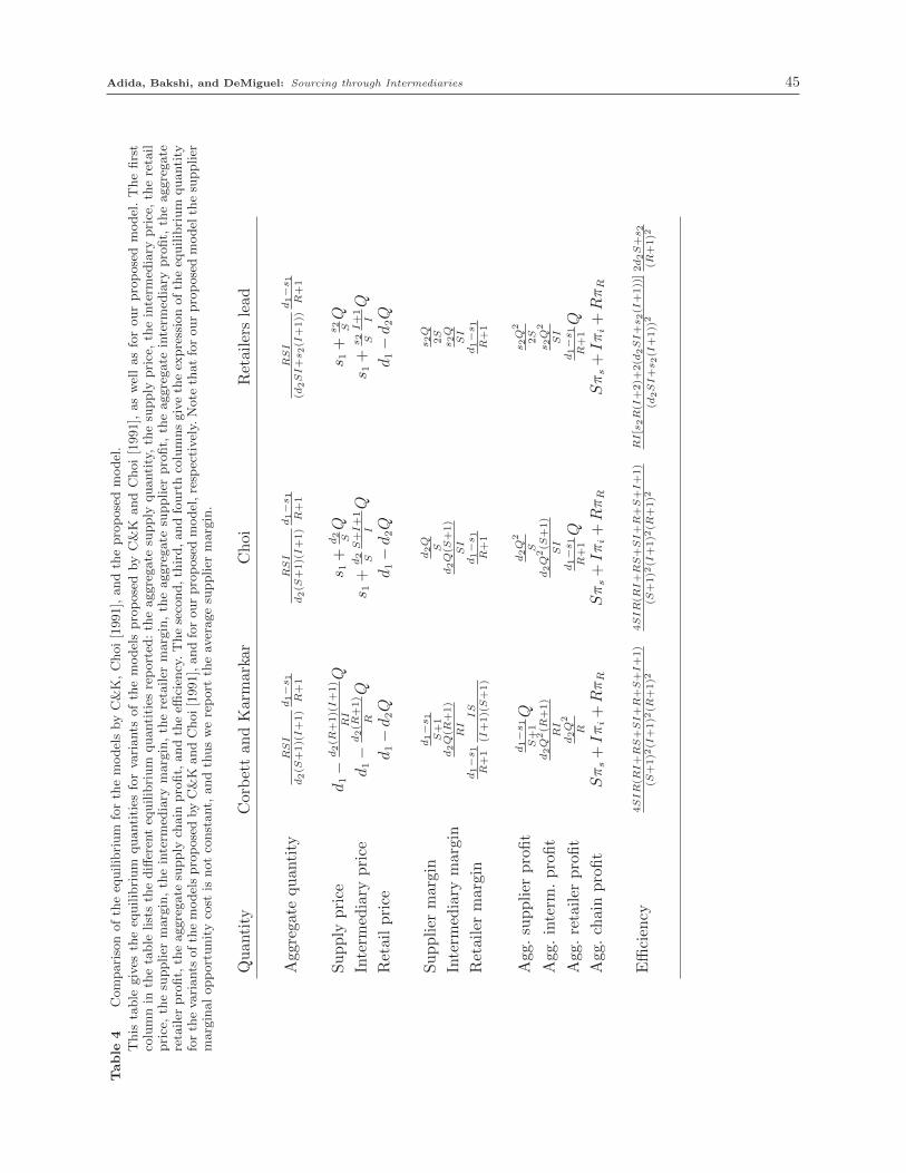
Adida, Bakshi, and DeMiguel: Sourcing through Intermediaries 45
Table
4Comparisonoftheequilibrium
forthemodelsbyC&K,Choi[1991],andtheproposedmodel.
This
table
gives
theequilibrium
quantities
forvariants
ofthemodelsproposedbyC&K
andChoi[1991],aswellasforourproposedmodel.Thefirst
columnin
thetable
liststhedifferen
tequilibrium
quantities
reported
:theaggregate
supply
quantity,thesupply
price,theinterm
ediary
price,theretail
price,thesupplier
margin,theinterm
ediary
margin,theretailer
margin,theaggregate
supplier
profit,
theaggregate
interm
ediary
profit,
theaggregate
retailer
profit,theaggregate
supply
chain
profit,andtheeffi
cien
cy.Thesecond,third,andfourthcolumnsgivetheexpressionoftheequilibrium
quantity
fortheva
riants
ofthemodelsproposedbyC&K
andChoi[1991],andforourproposedmodel,resp
ectively.
Note
thatforourproposedmodel
thesupplier
marginalopportunitycost
isnotconstant,
andthuswereport
theav
eragesupplier
margin.
Quan
tity
Corbettan
dKarmarkar
Choi
Retailerslead
Agg
rega
tequan
tity
RSI
d2(S
+1)(I+1)d1−s1
R+1
RSI
d2(S
+1)(I+1)d1−s1
R+1
RSI
(d2SI+s2(I
+1))
d1−s1
R+1
Supply
price
d1−
d2(R
+1)(I+1)
RI
Qs 1
+d2 SQ
s 1+
s2 SQ
Interm
ediary
price
d1−
d2(R
+1)
RQ
s 1+
d2 SS+I+1
IQ
s 1+
s2 SI+1
IQ
Retailprice
d1−d2Q
d1−d2Q
d1−d2Q
Supplier
margin
d1−s1
S+1
d2Q
Ss2Q
2S
Interm
ediary
margin
d2Q(R
+1)
RI
d2Q(S
+1)
SI
s2Q
SI
Retailer
margin
d1−s1
R+1
IS
(I+1)(S+1)
d1−s1
R+1
d1−s1
R+1
Agg
.supplier
profit
d1−s1
S+1Q
d2Q
2
Ss2Q
2
2S
Agg
.interm
.profit
d2Q
2(R
+1)
RI
d2Q
2(S
+1)
SI
s2Q
2
SI
Agg
.retailer
profit
d2Q
2
Rd1−s1
R+1Q
d1−s1
R+1Q
Agg
.chainprofit
Sπs+Iπi+RπR
Sπs+Iπi+RπR
Sπs+Iπi+RπR
Efficien
cy4SIR(R
I+RS+SI+R+S+I+1)
(S+1)2
(I+1)2
(R+1)2
4SIR(R
I+RS+SI+R+S+I+1)
(S+1)2
(I+1)2
(R+1)2
RI[s
2R(I
+2)+
2(d
2SI+s2(I
+1))]
(d2SI+s2(I
+1))
22d2S+s2
(R+1)2