southwest jiaotong university, chengdu, china arxiv:2011
TRANSCRIPT

RTFN: A Robust Temporal Feature Network for TimeSeries Classification
Zhiwen Xiaoa, Xin Xub, Huanlai Xinga,∗, Shouxi Luoa, Penglin Daia, DaweiZhana
aSouthwest Jiaotong University, Chengdu, ChinabChina University of Mining and Technology, Xuzhou, China
Abstract
Time series data usually contains local and global patterns. Most of the
existing feature networks pay more attention to local features rather than the
relationships among them. The latter is, however, also essential yet more diffi-
cult to explore. To obtain sufficient representations by a feature network is still
challenging. To this end, we propose a novel robust temporal feature network
(RTFN) for feature extraction in time series classification, containing a tempo-
ral feature network (TFN) and an LSTM-based attention network (LSTMaN).
TFN is a residual structure with multiple convolutional layers. It functions as
a local-feature extraction network to mine sufficient local features from data.
LSTMaN is composed of two identical layers, where attention and long short-
term memory (LSTM) networks are hybridized. This network acts as a relation
extraction network to discover the intrinsic relationships among the features
extracted from different data positions. In experiments, we embed RTFN into
a supervised structure as a feature extractor and an unsupervised structure as
an encoder, respectively. The results show that the RTFN-based structures
achieve excellent supervised and unsupervised performance on a large number
of UCR2018 and UEA2018 datasets.
Keywords: attention mechanism, convolutional neural network, data mining,
LSTM, time series classification.
∗Corresponding authorEmail address: [email protected] (Huanlai Xing)
Preprint submitted to Information Sciences January 1, 2021
arX
iv:2
011.
1182
9v2
[cs
.LG
] 2
9 D
ec 2
020

1. Introduction
Time series data has been used in various domains, such as weather fore-
casting [74], traffic analysis [40, 65], human activity recognition [2, 73], clinical
diagnosis [7], human heart record [10], electricity demand [46], etc. Making
full use of the data in real-world applications is crucial, depending on how well
features are extracted. Different from other types of data, such as ImageNet
for image classification [12], SemEval-2014 for sentiment recognition [44], and
ICDAR2019 for natural scene text processing [63], a time series is a sequence
of time-ordered data points recording certain processes [3]. In time series data,
local patterns are local temporal features, while global patterns are relation-
ships among local ones. Recently, effective feature and relation extraction has
become a critical challenge, which is also a basis for time series classification
[3, 15, 28, 36].
So far, there have been two classes of approaches for addressing the challenge
above, including traditional algorithms and deep learning ones [15]. Traditional
approaches aim at mining features and regularizations from data by revealing
the significant differences and connections within the data. These approaches
are mainly distance-based and feature-based. Distance-based approaches ad-
dress a classification task by measuring the similarities between spatial features
of data. Combining the nearest neighbor (NN) and the dynamic time warping
(DTW) is widely adopted [3, 33], such as, DDDTW [37], DTDC [37], DTWI
[13], DTWD [45], DTWA [36], etc. Besides, there are a number of NN-DTW-
based ensemble approaches. For example, the elastic ensemble (EE) uses 11
1-NN-based elastic distance measures to achieve decent performance on various
time series datasets [33]. The collective of transformation ensembles (COTE)
considers over 35 weighted classifiers [15]. In addition, the hierarchical vote
collective of transformation-based ensembles (HIVE-COTE) [34] and the local
cascade ensemble (LCE) [13] are two representative algorithms in the literature.
On the other hand, feature-based approaches pay more attention to exploring
2

representative features from time series data. For instance, Baydogan et al. [6]
introduce a bag-of-features framework for feature extraction via a truncated
discrete Fourier transform. The hidden state conditional random field (HCRF)
uses hidden variables to build the latent structure of the input [48]. Besides,
the learned pattern similarity (LPS) [5], the bag of SFA symbols (BOSS) [29],
the time series forest (TSF) [11], and the hidden unit logistic model (HULM)
[42] are also feature-based.
Apart from the distance- and feature-based approaches, research efforts have
also been dedicated to other techniques. For example, the ultra fast shapelets
(UFS) applies support vector machine and random forest to generate random
shapelets from the input [67]. The symbolic representation for multivariate time
series (SMTS) adopts random forest to divide time series data into leaf nodes
for local-pattern extraction [4]. Tuncel et al. [61] apply autoregressive forests
(mv-ARF) to mine representative shapelets from multivariate time series data.
Karlsson et al. [26] use generalized random shapelet forests (gRSF) to extract
significant features. WEASEL+MUSE utilizes a bag-of-patterns model with
various sliding window sizes for multivariate feature extraction [54].
On the other hand, the deep learning algorithms aim at unfolding the in-
ternal representation hierarchy of data, which helps to capture the intrinsic
connections among representations [31]. These algorithms are roughly classified
into two categories, namely single-network-based and dual-network-based mod-
els. To be specific, a single-network-based model uses one (usually hybridized)
network to handle both feature and relation extraction. These models pay at-
tention to mining the basic representation hierarchy of data and significant con-
nections within the hierarchy, e.g., ConvTimeNet [27], InceptionTime [16], and
OmniScale 1-dimensional convolutional neural network (OS-CNN) [60]. A dual-
network-based model is composed of a local-feature extraction network and a
relation extraction network in parallel. The first network, usually convolutional
structure based, concentrates on local features. In contrast, the second one
focuses on relationships among the features extracted, e.g. Transformer-based
model [23], ALSTM-FCN [24], etc. Compared with feature extraction, rela-
3

tion extraction aims at capturing those hidden connections among the features
extracted before. In other words, a relation extraction network is able to com-
pensate for the loss of the representations ignored by its corresponding feature
extraction network. Hence, it is vital to design an effective relation extraction
network for different applications [3, 15, 23]. Nowadays, attention and long
short-term memory (LSTM) networks are widely used for relation extraction in
time series classification. That is because the attention mechanism can relate
different positions of a sequence to derive the relationships at certain positions
[62] and LSTM is able to explore long- and short-period dependencies in data,
both of which help to enhance the relation extraction [8, 20, 24].
Nowadays, hybridizing attention and LSTM networks for relation extraction
has attracted increasingly more research attention in time series classification.
There are mainly two ways to combine them, namely cascading and embedding
models. A cascading model stacks attention and LSTM networks one after an-
other to realize some specific functions. But, neither attention networks nor
LSTM networks require significant changes in their structures, e.g. the atten-
tion LSTM (AttLSTM) models [24, 25]. However, the cascading models usually
suffer from two drawbacks. Firstly, almost all attention networks are based on
fully connected networks, which are not sensitive to the intricate features hid-
den in data. Secondly, the useful representations extracted before are easily lost
as they go through subsequent networks. An embedding model, on the other
hand, integrates attention and LSTM networks in a compact manner. With
fewer layers of neural networks cascaded, fewer features are lost during data
transmission. Thus, more useful features and relationships are made use of by
the model. Such a model is sensitive to regular and periodic data and hence able
to concentrate on the local and periodical variations of data, e.g., LSTM with
trend attention gate (LSTMTAG) [35]. If not designed properly, an embedding
model may not be aware of the global variations of those non-periodical data, es-
pecially when handling long univariate and multivariate datasets. Theoretically
speaking, compared with fully connected networks, embedding LSTM networks
into an attention structure helps to provide it with significantly more tempo-
4

ral features for calculation, improving its sensitivity to the global variations of
non-periodical data. Unfortunately, such a structure has not been considered
in the time series data mining community.
To take advantage of the dual-network-based model and the hybridization of
attention and LSTM networks, we propose a robust temporal feature network
(RTFN) for feature extraction in the area of time series classification. RTFN
consists of a temporal feature network as its local-feature extraction network
and an LSTM-based attention network as its relation extraction network. Our
main contributions are summarized below.
- The temporal feature network is a CNN-based residual structure, respon-
sible for extracting sufficient local features. Multi-head CNN layers are
used to diversify multi-scale features, and self-attention is adopted to re-
late different positions of the features extracted before. Besides, we use
the leaky rectified linear unit as the activation function to reduce the loss
of features during their transmission.
- The LSTM-based attention network contains two identical layers. In each
layer, instead of fully connected networks, LSTM networks are used to
obtain the query, key, and value matrices for their corresponding atten-
tion structure. Unlike the existing structures that combine attention and
LSTM networks, the LSTM-based attention network can pay attention to
the global variations of non-periodical data, which helps to mine useful
relationships among the features already learned.
- We embed RTFN into a supervised structure and test it on 85 UCR2018
datasets and 30 UEA2018 datasets, where the RTFN-based algorithm out-
performs a number of existing supervised algorithms on 39 UCR2018 and
15 UEA2018 datasets, respectively. Also, we embed RTFN into a simple
unsupervised clustering as an encoder. Our structure wins 9 out of 36
UCR2018 datasets, compared with 13 unsupervised algorithms.
The rest of the paper is organized as follows. Section 2 reviews the state-of-
the-art deep learning algorithms for time series classification and various com-
binations of attention and LSTM networks. Section 3 introduces the overview
5

of RTFN, its key components, the RTFN-based supervised structure, and the
RTFN-based unsupervised clustering. Experimental results are given in Section
4. Section 5 concludes the paper.
2. Related Work
This section first reviews the deep learning algorithms for time series classi-
fication and then discusses the existing means to hybridize attention and LSTM
networks.
2.1. Deep Learning Algorithms
Since the introduction of the fully convolutional network (FCN) [66], increas-
ingly more algorithms have been proposed to address time series classification
problems [15]. In general, these algorithms are either single-network-based or
dual-network-based. Single-network-based algorithms focus on significant fea-
tures of data. For example, a 34-layer convolutional neural network was con-
structed to handle the ECG classification problem [49]. Serra et al. developed a
universal encoder based on CNN and convolutional attention to mine the tem-
poral representations from input data [55]. In [27], an off-the-shelf deep CNN
(ConvTimeNet) with four convolutional blocks was proposed as a transferable
network to adapt quickly for the requirements of datasets. Fawaz et al. used
a fast gradient sign method to fool a ResNet model, called adversarial attacks
for time series classification, where a set of synthetic samples was generated
[14]. Besides, InceptionTime [16], and OS-CNN [60] are often regarded as two
representative single-network-based models, achieving decent performance on
many univariate time series datasets. InceptionTime uses an inception struc-
ture to explore multi-scale representations from data, and OS-CNN adopts 1-
dimensional CNN to mine local features and the relationships among the data.
On the other hand, as an emerging trend for time series classification, dual-
network-based models have not yet received much research attention. A few
LSTM-FCN-based models were designed to cope with univariate and multivari-
ate time series classification problems[24, 25], where FCN and LSTM were used
6

for feature and relation extraction, respectively. In [23], Huang et al. proposed a
residual attention net (RAN) consisting of a ResNet-based feature network and
a transformer-based relation network, obtaining promising performance on UCR
datasets. Meanwhile, the dual-network-based algorithms usually achieved bet-
ter classification performance than those single-network-based ones [23, 24, 25].
2.2. Hybridization of Attention and LSTM
Hybridizing attention and LSTM models is an emerging solution to tempo-
ral and spatial relation extraction. The existing works mainly include cascading
and embedding models. The former simply stacks attention and LSTM struc-
tures together. For instance, an attention-LSTM model was adopted to cope
with univariate and multivariate time series classification on UCR and UEA
datasets, respectively [24, 25]. An attention-LSTM model was integrated into
the convolution–deconvolution word embedding to merge context-specific and
task-specific information [58]. In [71], an attention-based time-incremental CNN
cascaded attention and LSTM networks for temporal and spatial information
fusion of ECG signals. Besides, the cascading models have been applied to video
segmentation [64], semantic relation extraction [18], visual question answer [75],
urban flow prediction [52], and so on. On the other hand, the embedding models
focus on the compact integration of attention and LSTM networks. For instance,
a TAG-embedded LSTM model was devised to explore the local variations of
quasi-periodic time series data [35]. Wang et al. [77] proposed a novel online
attentional recurrent neural network (ARNN) model for video tracking, where
inter- and intra-attention models were embedded into a bi-directional LSTM to
distinguish different background scenarios. In [9], Chen et al. put forward an
identity-aware single shot multi-boxes detector for object detection, where an
attention-embedded LSTM structure was used to locate positions of interest-
ing objects. In [59], an attention-based LSTM was introduced to capture the
representation hierarchy of data in power consumption forecasting.
7

2.3. Analysis and Motivation
The dual-network-based models realize feature and relation extraction by
two separate networks in parallel. Such a model usually performs better than a
single-network-based model in supervised classification and unsupervised clus-
tering, according to references [23, 24, 25] and our observations in Section 4.4.
Nevertheless, designing a dual-network-based model is quite challenging since its
structure should meet datasets’ requirements, especially its relation extraction
network. The hybridization of attention and LSTM offers a promising means to
discover the relationships among the representations obtained from data. But,
the existing cascading and embedding models cannot well handle the global
variations of non-periodical time series data. The above is the motivation why
we design a dual-network-based algorithm for time series classification and why
we embed LSTM into an attention structure for relation extraction.
3. RTFN
This section first overviews the structure of RTFN and then describes two
important components, namely a convolutional neural block and an LSTM-
based attention layer. In the end, the RTFN-based supervised structure and
unsupervised clustering are introduced, respectively.
3.1. Overview
The structure of RTFN is shown in Fig. 1. It primarily consists of a temporal
feature network (TFN) and an LSTM-based attention network (LSTMaN). In
TFN, a convolutional neural block, namely ’Conv1D’, is seen as a basic building
block responsible for capturing the local features from the input. Two multi-
head convolutional neural layers, each consisting of four Conv1D blocks, are
used to discover higher-level multi-scale features from the lower-level features
extracted before. Besides, we place a self-attention layer [62] between the two
multi-head layers to relate the positions of the local features obtained by the
first multi-head layer, which enriches the input features of the second multi-
head layer. Detailed observations can be found in Section 4.3. LSTMaN is
8

Figure 1: Structure of RTFN.
composed of two LSTM-based attention layers, aiming at digging out the in-
trinsic relationships among the features learned from the input, which helps to
compensate for the loss of the representations ignored by TFN. TFN and LST-
MaN are used as the local-feature and relation extraction networks, respectively.
Combining them provides RTFN with sufficient features and relationships. In
this paper, RTFN is embedded into a supervised structure in Section 3.4 and
an unsupervised clustering in Section 3.5, respectively.
3.2. Convolutional Neural Block (Conv1D)
A Conv1D block consists of a 1-dimensional CNN module, a batch normal-
ization module, and a leaky rectified linear unit (LeakReLU) activation function
[51], as defined in Eq. (1).
OConv1D = fLeakReLU (fBN (fconv(x))) (1)
where, OConv1D and x are the output and input of the Conv1D block, respec-
tively. fLeakReLU , fBN , and fconv denote the LeakReLU activation, batch
normalization, and CNN functions, respectively.
9

The CNN module is used to explore the local features from the input [31],
as defined in Eq. (2).
fconv(x) = Wcnn ⊗ x+ bcnn (2)
where, Wcnn and bcnn are the weight and bias matrices of CNN, respectively.
⊗ is the convolutional computation operation.
Let xbn = {a1, a2, ..., aN} be the input of the batch normalization module,
where ai and N are the i-th instance and the batch size, respectively. Let
µ = 1N
∑Ni=1 ai and δ =
√1N
∑Ni=1 (ai − µ)2 denote the mean and standard
deviation of xbn, respectively. fBN (xbn) is defined in Eq. (3).
fBN (a1, a2, ..., aN ) = (γa1 − µδ + ε
+ β, γa2 − µδ + ε
+ β, ..., γaN − µδ + ε
+ β) (3)
where, γ ∈ R+ and β ∈ R are the parameters to be learned during training and
ε>0 is an arbitrarily small number.
The batch normalization module eliminates the internal covariate shift and
thus ensures a faster training process. Also, it regularizes the proposed model
and enhances its local-feature extraction ability in supervised classification and
unsupervised clustering. Meanwhile, different from the rectified linear unit
(ReLU) that only considers positive numbers, LeakReLU takes care of both
positive and negative numbers, reducing the loss of features during the data
transmission process. Detailed observations are shown in Section 4.3. The
LeakReLU activation is defined in Eq. (4).
fLeakReLU (xactv) =
αxactv, xactv<0
xactv, xactv ≥ 0
(4)
where, xactv is the input of the LeakReLU unit and α is a coefficient for negative
numbers. Following the widely recognized YOLOv3 [51], we set α = 0.1 in this
paper.
3.3. LSTM-based attention Layer
As aforementioned, LSTMaN is proposed for relation extraction, including
two LSTM-based attention layers. The two layers have the same structure, as
10

shown in Fig. 2, where ’MatMul’ is a matrix multiplication operation. The first
layer is used to extract basic relationships from the input, while the second layer
is responsible for mining the intricate connections among them. By extending
the details of the relationships obtained before, the second layer helps to extract
more complex regularizations hidden in data than the first layer.
Figure 2: Structure of the LSTM-based attention layer.
Unlike the existing models that hybridize attention and LSTM networks (see
Section 2.2), an LSTM-based attention layer incorporates LSTM networks into
an attention structure. In this network, a temporal query and a set of key-
value pairs are mapped to an output, where Query, Key, and Value are matrices
obtained from the feature extraction by the LSTM networks. The output is
defined as a weighted sum of the values with sufficient representations. In this
paper, each value is obtained by a compatibility function that mines the hidden
relationships between a query and its corresponding key that already carry
basic features. The query, key, and value matrices output by the three LSTM
networks, Iq, Ik, Iv, are defined in Eqs. (5), (6) and (7), respectively.
Iq = fLSTM−Q(x) (5)
Ik = fLSTM−K(x) (6)
Iv = fLSTM−V (x) (7)
where, x is the input of the layer and fLSTM−Q, fLSTM−K and fLSTM−V are the
LSTM functions for obtaining the query, key, and value matrices, respectively.
Note that each of the three LSTM networks involves the same computational
procedure at time step t as a traditional LSTM network [22]. The following
11

describes the computation operations in an LSTM network. Let xt and ht be the
input vector and the hidden state vector of the LSTM network at t, respectively.
Let gut , gft , got , and gct are the activation vectors of the input, forget, output, and
cell state gates at t, respectively. Denote the elementwise multiplication by �.
Let σ and tanh denote the logistic sigmoid and hyperbolic tangent functions,
respectively. Let Wux, Wfx, Wox, and Wcx be the weight matrices of xt at gates
gut , gft , got , and gct , respectively. Let Wuh, Wfh, Woh, and Wch denote the weight
matrices of ht at gates gut , gft , got , and gct , respectively. Let bu, bf , bo, and bc be
the bias matrices of ht at gates gut , gft , got , and gct , respectively. gut , gft , got , gct ,
and ht are defined in Eqs. (8)-(12), respectively.
gut = σ(Wuxxt +Wuhht−1 + bu) (8)
gft = σ(Wfxxt +Wfhht−1 + bf ) (9)
got = σ(Woxxt +Wohht−1 + bo) (10)
gct = gft � gct−1 + gut � tanh(Wcxxt +Wchht−1 + bc) (11)
ht = got � tanh(gct ) (12)
After x goes through the LSTM networks, Iq, Ik, and Iv carry sufficient
long- and short-term features. They are then fed into the attention structure,
and its output matrix, OAtt, is defined in Eq. (13).
OAtt = fSoftMax(Iq · ITk ) · Iv (13)
where, fSoftMax is a commonly used function to compute the possibilities of a
certain matrix, and ITk is the transpose of Ik.
Note that we concatenate the local features obtained by TFN and the global
relationships obtained by LSTMaN in RTFN. Let OTFN and OLSTMaN denote
the output matrices of TFN and LSTMaN, respectively. The output of RTFN,
ORTFN , is defined in Eq. (14).
ORTFN = fconcat([OTFN , OLSTMaN ]) (14)
where, fconcat is the CONCAT function.
12
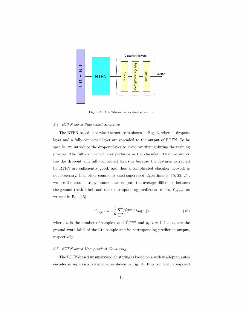
Figure 3: RTFN-based supervised structure.
3.4. RTFN-based Supervised Structure
The RTFN-based supervised structure is shown in Fig. 3, where a dropout
layer and a fully-connected layer are cascaded to the output of RTFN. To be
specific, we introduce the dropout layer to avoid overfitting during the training
process. The fully-connected layer performs as the classifier. That we simply
use the dropout and fully-connected layers is because the features extracted
by RTFN are sufficiently good, and thus a complicated classifier network is
not necessary. Like other commonly used supervised algorithms [3, 15, 23, 25],
we use the cross-entropy function to compute the average difference between
the ground truth labels and their corresponding prediction results, Lsuper, as
written in Eq. (15).
Lsuper = − 1
n
n∑i=1
(Y traini log(pi)) (15)
where, n is the number of samples, and Y traini and pi, i = 1, 2, ..., n, are the
ground truth label of the i-th sample and its corresponding prediction output,
respectively.
3.5. RTFN-based Unsupervised Clustering
The RTFN-based unsupervised clustering is based on a widely adopted auto-
encoder unsupervised structure, as shown in Fig. 4. It is primarily composed
13

Figure 4: RTFN-based unsupervised clustering.
of an RTFN-based encoder, a decoder, and a K-means algorithm [21]. RTFN
is responsible for obtaining as many useful representations from the input as
possible. The decoder is made up of four fully-connected layers, helping to
reconstruct the features captured by RTFN. Besides, the K-means algorithm
acts as the unsupervised classifier.
Different from taking the k-means loss into account [19, 36, 39], the RTFN-
based unsupervised clustering only depends on the reconstruction loss (i.e., the
mean square error), Lrec, as defined in Eq. (16).
Lrec =1
n
n∑i=1
(Xtraini −Xrec
i )2 (16)
where Xtraini and Xrec
i , i = 1, 2, ..., n, are the input and the decoder output of
the i-th sample, respectively.
No matter the supervised or unsupervised structure, our goal is to minimize
its loss function, L, by finding the optimal parameters, θ∗, where L(θ∗) is in-
finitely close to 0. This paper uses the gradient-descent method to approximate
θ∗ for our proposed structure. Let θt and lrate denote the parameters and the
learning rate at the t-th training epoch, respectively. θt is updated by Eq. (17).
θt = θt−1 − lrate∇θt−1L(θt−1) (17)
where, ∇θt−1represents the gradient at the (t− 1)-th training epoch.
14

4. Experiments and Analysis
This section first introduces the experimental setup and performance metrics
and then focus on the ablation study. Finally, the RTFN-based supervised
structure and unsupervised clustering are evaluated, respectively.
4.1. Experimental Setup
Extensive experiments in supervised classification and unsupervised cluster-
ing have been conducted. This section introduces the standard datasets first
and the implementation details later.
Supervised Classification Datasets. A univariate time series refers to
a series of time-ordered data points associated with a time-dependent variable.
Such a sequence contains local and global patterns of data. Local patterns show
significant changes in the data, and global patterns reflect the overall trend of
data [10]. A multivariate time series consists of multiple concurrent univariate
time series, each associated with a time-dependent variable. Like univariate
time series, a multivariate time series also contain local and global pattern
information. Besides, as each variable has some dependency on other variables,
a multivariate time series contains relationship information between variables
[2]. In the supervised area, time series data are labeled. A supervised algorithm
learns the characteristics of the input data and maps the data to labels. For
a univariate time series, a supervised algorithm needs to mine the local and
global patterns from the data, such as EE [33], COTE [15], LPS [5], LCE [13],
ConvTime [27], ResNet-Transformer models [23], etc. For a multivariate time
series, a supervised algorithm focuses on not only the local and global patterns
of each variable but also the relationships between variables, e.g., HUML [42],
SMTS [4], mv-ARF [61], WEASEL + MUSE [54], TapNet [76], FCN-MLSTM
[25], and so on.
We evaluate the performance of the RTFN-based supervised structure by a
number of univariate and multivariate time series datasets. For the univariate
time series, UCR2018 [10] is one of the authoritative data archives, which con-
tains 128 datasets with different lengths in a variety of application areas. We
15

Table 1: Details of 85 univariate time series datasets. Those marked with ’YES’ are also used
for unsupervised clustering experiments.Dataset TrainSize TestSize Classes SeriesLength Type Unsupervised
Adiac 390 391 37 176 Image
ArrowHead 36 175 3 251 Image YES
Beef 30 30 5 470 Spectro YES
BeetleFly 20 20 2 512 Image YES
BirdChicken 20 20 2 512 Image YES
Car 60 60 4 577 Sensor YES
CBF 30 900 3 128 Simulated
ChlorineConcentration 467 3840 3 166 Sensor YES
CinCECGTorso 40 1380 4 1639 Sensor
Coffee 28 28 2 286 Spectro YES
CricketX 390 390 12 300 Motion
CricketY 390 390 12 300 Motion
CricketZ 390 390 12 300 Motion
DiatomSizeReduction 16 306 4 345 Image YES
DistalPhalanxOutlineAgeGroup 400 139 3 80 Image YES
DistalPhalanxOutlineCorrect 600 276 2 80 Image YES
Earthquakes 322 139 2 512 Sensor
ECG200 100 100 2 96 ECG YES
ECG5000 500 4500 5 140 ECG
ECGFiveDays 23 861 2 136 ECG YES
FaceFour 24 88 4 350 Image
FacesUCR 200 2050 14 131 Image
FordA 3601 1320 2 500 Sensor
FordB 3636 810 2 500 Sensor
GunPoint 50 150 2 150 Motion YES
Ham 109 105 2 431 Spectro YES
HandOutlines 1000 370 2 2709 Image
Haptics 155 308 5 1092 Motion
Herring 64 64 2 512 Image YES
InlineSkate 100 550 7 1882 Motion
InsectWingbeatSound 220 1980 11 256 Sensor
ItalyPowerDemand 67 1029 2 24 Sensor
Lightning2 60 61 2 637 Sensor YES
Lightning7 70 73 7 319 Sensor
Mallat 55 2345 8 1024 Simulated
Meat 60 60 3 448 Spectro YES
MedicalImages 381 760 10 99 Image
MiddlePhalanxOutlineAgeGroup 400 154 3 80 Image YES
MiddlePhalanxOutlineCorrect 600 291 2 80 Image YES
MiddlePhalanxTW 399 154 6 80 Image YES
MoteStrain 20 1252 2 84 Sensor YES
OliveOil 30 30 4 570 Spectro
OSULeaf 200 242 6 427 Image YES
Plane 105 105 7 144 Sensor YES
ProximalPhalanxOutlineAgeGroup 400 205 3 80 Image YES
ProximalPhalanxOutlineCorrect 600 291 2 80 Image
ProximalPhalanxTW 400 205 6 80 Image YES
ShapeletSim 20 180 2 500 Simulated
ShapesAll 600 600 60 512 Image
SonyAIBORobotSurface1 20 601 2 70 Sensor YES
SonyAIBORobotSurface2 27 953 2 65 Sensor YES
Strawberry 613 370 2 235 Spectro
SwedishLeaf 500 625 15 128 Image YES
Symbols 25 995 6 398 Image YES
SyntheticControl 300 300 6 60 Simulated
ToeSegmentation1 40 228 2 277 Motion YES
ToeSegmentation2 36 130 2 343 Motion YES
Trace 100 100 4 275 Sensor
TwoPatterns 1000 4000 4 128 Simulated YES
TwoLeadECG 23 1139 2 82 ECG YES
UWaveGestureLibraryAll 896 3582 8 945 Motion
UWaveGestureLibraryX 896 3582 8 315 Motion
UWaveGestureLibraryY 896 3582 8 315 Motion
UWaveGestureLibraryZ 896 3582 8 315 Motion
Wafer 1000 6164 2 152 Sensor YES
Wine 57 54 2 234 Spectro YES
WordSynonyms 267 638 25 270 Image YES
ACSF1 100 100 10 1460 Device
BME 30 150 3 128 Simulated
Chinatown 20 345 2 24 Traffic
Crop 7200 16800 24 46 Image
DodgerLoopDay 78 80 7 288 Sensor
DodgerLoopGame 20 138 2 288 Sensor
DodgerLoopWeekend 20 138 2 288 Sensor
GunPointAgeSpan 135 316 2 150 Motion
GunPointMaleVersusFemale 135 316 2 150 Motion
GunPointOldVersusYoung 136 315 2 150 Motion
InsectEPGRegularTrain 62 249 3 601 EPG
InsectEPGSmallTrain 17 249 3 601 EPG
MelbournePedestrian 1194 2439 10 24 Traffic
PowerCons 180 180 2 144 Power
Rock 20 50 4 2844 Spectrum
SemgHandGenderCh2 300 600 2 1500 Spectrum
SemgHandMovementCh2 450 450 6 1500 Spectrum
SemgHandSubjectCh2 450 450 5 1500 Spectrum
SmoothSubspace 150 150 3 15 Simulated
UMD 36 144 3 150 Simulated
16

Table 2: Details of 30 multivariate time series datasets. Abbreviations: AS - Audio Spectra,
ECG - Electrocardiogram, EEG - Electroencephalogram, HAR - Human Activity Recognition,
MEG - Magnetoencephalography.
Index Dataset TrainSize TestSize NumDimensions SeriesLength Classes Type
AWR ArticularWordREcognition 275 300 9 144 25 Motion
AF AtrialFibrillation 15 15 2 640 3 ECG
BM BasicMotions 40 40 6 100 4 HAR
CT CharacterTrajectories 1422 1436 3 182 20 Motion
CR Critcket 108 72 6 1197 12 HAR
DDG DuckDuckGeese 50 50 1345 270 5 AS
EW EigenWorm 128 131 6 17894 4 Motion
EP Epliyepsy 137 138 3 206 4 HAR
EC EthanolConcentration 261 263 3 1751 4 HAR
ER ERing 30 270 4 65 6 Other
FD FaceDetection 5890 3524 144 62 2 EEG/MEG
FM FingerMovements 316 100 28 50 2 EEG/MEG
HMD HandMovementDirection 160 74 10 400 4 EEG/MEG
HW Handwriting 150 850 3 152 26 HAR
HB Heartbeat 204 205 61 405 2 AS
IW InsectionWingbeat 30000 20000 200 30 10 AS
JV JapaneseVowels 270 370 12 29 9 AS
LIB Libras 180 180 2 45 15 HAR
LSST LSST 2459 2466 6 36 14 Other
MI MotorImagery 278 100 64 3000 2 EEG/MEG
NATO NATOPS 180 180 24 51 6 HAR
PD PenDigits 7494 3498 2 8 10 EEG/MEG
PEMS PEMSF 267 173 963 144 7 EEG/MEG
PS Phoneme 3315 3353 11 217 39 AS
RS RacketSports 151 152 6 30 4 HAR
SRS1 SelfRegulationSCP1 268 293 6 896 2 EEG/MEG
SRS2 SelfRegulationSCP2 200 180 7 1152 2 EEG/MEG
SAD SpokenArbicDigits 6599 2199 13 93 10 AS
SWJ StandWalkJump 12 15 4 2500 3 ECG
UW UWaveGuestureLibrary 120 320 3 315 8 HAR
select 85 standard datasets from the UCR2018 archive, consisting of 65 ’short-
medium’ and 20 ’long’ time series datasets. In this paper, a ’long’ dataset is
a dataset with a length of over 500. The details of these datasets are shown
in Table 1. As for the multivariate time series, UEA2018 [2] is a commonly
used data archive, including 30 datasets in seven application areas, i.e., audio
spectra, electrocardiogram, electroencephalogram, human activity recognition,
motion, eagnetoencephalography and other. Their details are listed in Table 2.
Unsupervised Clustering Datasets. In the unsupervised area, time se-
ries data are not labeled. An unsupervised algorithm discovers the previously
undetected patterns in a dataset. For a univariate time series, an unsupervised
algorithm aims to learn the underlying structure or distribution in the data,
17

such as K-means [21], UDFS [70], K-shape [41], DTCR [36], IDEC [19], etc.
For a multivariate time series, an unsupervised algorithm learns not only the
underlying structure or distribution of each variable but also the relationships
between variables, e.g., USAD [1].
Following the protocol used in [19, 36, 39], we verify the performance of the
RTFN-based unsupervised clustering by 36 standard datasets selected from the
UCR2018 archive. They are marked with ’YES’ in column ’Unsupervised’ in
Table 1.
Implementation Details. Firstly, we introduce the parameter settings for
TFN. As mentioned in Section 3.2, each Conv1D block contains a 1-dimensional
CNN module. In the Conv1D block directly connected to the residual junction,
the 1-dimensional CNN module also has 128 channels, each with a kernel size
of 1. In each multi-head Conv1D layers, each of the four 1-dimensional CNN
modules has 32 channels. Motivated by InceptionTime [16], we set the kernel
sizes of the four CNN modules to 5, 8, 11, and 17, respectively. Following the
previous works in [8, 20, 23, 51], we set the decay value of the batch normal-
ization module to 0.9, which helps to accelerate the training by reducing the
internal covariate shift of time series data.
In the two Conv1D blocks next to the input of RTFN, each 1-dimensional
CNN module has 128 channels, each with a kernel size of 11. The following
explains why 11 is chosen. As references [16, 23, 24, 27, 60, 66] suggest, we
choose 3, 5, 7, 9, 11, and 13 as the candidate kernel sizes for the two Con-
vlD blocks above. We select eight univariate and four multivariate datasets
from the UCR2018 and UEA2018 archives, respectively. The eight univariate
datasets contain four ‘short-medium’ and four ‘long’ time series datasets. Table
3 shows the top-1 accuracy results with six different kernel sizes used in the two
Conv1D blocks. A larger kernel size usually leads to higher accuracies because
such a kernel has a broader receptive field and thus captures richer local features.
Clearly, kernel sizes 11 and 13 result in better performance than 3, 5, 7, and
9. Kernel sizes 11 and 13 lead to similar accuracy results on each dataset. On
the other hand, a larger kernel size means the corresponding convolutional op-
18

erations consume more computing resources. To compromise between accuracy
and complexity, we set the kernel size of the two Conv1D blocks to 11.
Table 3: Results of the top-1 accuracy vs. the kernel size.Type Dataset Kernel size = 3 Kernel size = 5 Kernel size = 7 Kernel size = 9 Kernel size = 11 Kernel size = 13
Univariate Time Series
ECG200 0.9 0.91 0.91 0.92 0.92 0.93
Lighting7 0.863014 0.876712 0.890411 0.90411 0.90411 0.90411
Ham 0.761905 0.761905 0.780952 0.780952 0.809524 0.809524
Wine 0.87037 0.87037 0.888889 0.888889 0.907407 0.907407
SemgHandGenderCh2 0.876667 0.96 0.91 0.913333 0.923333 0.923333
SemgHandMovementCh2 0.6 0.616667 0.66667 0.716667 0.757778 0.757778
SemgHandSubjectCh2 0.788889 0.816667 0.833333 0.85 0.897778 0.897778
Rock 0.84 0.84 0.84 0.86 0.88 0.88
MeanACC 0.812606 0.831540 0.840032 0.854244 0.874991 0.876241
Multivariate Time Series
AF 0.467 0.467 0.533 0.533 0.533 0.533
FD 0.629 0.631 0.649 0.656 0.67 0.67
HMD 0.649 0.649 0.662 0.662 0.662 0.662
HB 0.727 0.748 0.751 0.751 0.785 0.785
MeanACC 0.618 0.624 0.649 0.651 0.663 0.663
Secondly, we introduce the parameter settings for LSTMaN. As described
in Section 3.3, there are two LSTM-based attention layers. In each layer, as
references [24, 25] suggest, we set the number of hidden units in each LSTM
network to 128.
Last but not least, we dynamically adjust the learning rate during the train-
ing process. Let the total number of training epochs and the size of each decay
period denoted by Ntot and Ndec, respectively. Let lrate(j), j = 1, 2, ..., J , de-
note the learning rate of the j − th decay period, where J = dNtot/Ndece − 1.
Its definition is written in Eq. (18).
lrate(j) = (1− drate)× lrate(j − 1) (18)
where drate and J are the decay rate of lrate and the total number of the decay
periods, respectively. In this paper, we set lrate(0) = 0.01 and drate = 0.1.
Once lrate is smaller than 0.0001, we fix it to 0.0001. The RMSPropOptimizer
of Tensorflow 1 is used to tune the parameters of our proposed RTFN structures
for supervised classification and unsupervised clustering. According to [53], we
set the RMSPropOptimizer’s momentum term to 0.9 to avoid falling into local
minima during training. Besides, we use the dropout layer and L2 regularization
1https://tensorflow.google.cn/
19
to avoid overfitting during the training process. As references [8, 49, 52, 75, 77]
suggest, the dropout layer’s ratio value is set to 0.5.
All experiments are run on a computer with Ubuntu 18.04 OS, an Nvidia
GTX 1070Ti GPU with 8GB, an Nvidia GTX 1080Ti GPU with 11GB, and an
AMD R5 1400 CPU with 16G RAM.
4.2. Performance Metrics
To evaluate the performance of various algorithms in terms of supervised
classification and unsupervised clustering, we adopt a number of well-known
performance metrics explained below.
Supervised Classification. Three metrics are used to rank different su-
pervised algorithms in terms of the top-1 accuracy, including ‘win’/‘tie’/‘lose’,
mean accuracy (MeanACC), and AVG rank. To be specific, for an arbitrary
algorithm, its ‘win’, ‘tie’, and ‘lose’ values indicate on how many datasets this
algorithm performs better than, equivalent to, and worse than the others, re-
spectively. For each algorithm, the ‘best’ value is the summation of its cor-
responding ‘win’ and ‘tie’ values, while the ‘total’ value is the total number
of datasets tested. In addition, the AVG rank score measures the average dif-
ference between the accuracy values of a model and the best accuracy values
among all models [15, 13, 38, 23].
Unsupervised Clustering. Note that the top-1 accuracy is not applica-
ble to unsupervised clustering. Instead, we use a widely adopted performance
indicator, the rand index (RI) [50], RI, as defined in Eq. (19).
RI =PTP +NTP
s(s− 1)/2(19)
where PTP and NTP are the numbers of the positive and negative time series
pairs in the clustering, respectively, and s is the dataset size. Besides, we denote
the average RI value of a certain algorithm by ‘AVG RI’.
4.3. Ablation Study
As shown in Fig. 1, RTFN mainly consists of a temporal feature network
for local-feature extraction, i.e., TFN, and an LSTM-based attention network
20

for relation extraction, i.e., LSTMaN.
Table 4: The top-1 accuracy results of different supervised algorithms on 12 selected datasets.Type Dataset SeriesLength TFN TFN w ReLU TFN w/o SelAtt TFN+1LSTMaL TFN+2LSTMaL TFN+3LSTMaL TFN+AttLSTM TFN+LSTMTAG
Univariate Time
Series
ECG200 96 0.84 0.82 0.8 0.9 0.92 0.92 0.91 0.89
Lighting7 319 0.821918 0.808219 0.808219 0.849315 0.90411 0.90411 0.849315 0.849315
Ham 431 0.714286 0.619048 0.619048 0.761905 0.809524 0.809524 0.780952 0.761905
Wine 234 0.833333 0.611111 0.555556 0.888889 0.907407 0.907407 0.888889 0.87037
SemgHandGenderCh2 1500 0.796667 0.783333 0.651667 0.866667 0.923333 0.923333 0.91 0.84
SemgHandMovementCh2 1500 0.595555 0.56 0.513333 0.611111 0.757778 0.757778 0.56 0.56
SemgHandSubjectCh2 1500 0.793333 0.788889 0.74 0.8 0.897778 0.897778 0.873333 0.74
Rock 2844 0.7 0.64 0.62 0.82 0.88 0.88 0.86 0.68
MeanACC 0.761887 0.703825 0.663478 0.812236 0.874991 0.874991 0.829061 0.773949
Multivariate Time
Series
AF 640 0.4 0.333 0.267 0.467 0.533 0.533 0.467 0.2
FD 62 0.555 0.545 0.519 0.614 0.67 0.67 0.631 0.555
HMD 400 0.544 0.481 0.5 0.649 0.662 0.662 0.649 0.649
HB 405 0.547 0.535 0.515 0.761 0.785 0.785 0.727 0.547
MeanACC 0.512 0.474 0.450 0.623 0.663 0.663 0.619 0.488
Table 5: The RI results of different unsupervised algorithms on four selected datasets.
Dataset TFN TFN w ReLU TFN w/o SelAtt TFN+1LSTMaL TFN+2LSTMaL TFN+3LSTMaL TFN+AttLSTM TFN+LSTMTAG
Beef 0.6267 0.5945 0.5402 0.7034 0.7655 0.7655 0.7057 0.7034
Car 0.6418 0.6354 0.626 0.6708 0.7169 0.7028 0.6898 0.6418
ECG200 0.6533 0.6315 0.6018 0.7018 0.7285 0.7285 0.7018 0.7018
Lighting2 0.5373 0.5119 0.4966 0.5729 0.6230 0.6230 0.5770 0.5770
AVG RI 0.6148 0.5933 0.5662 0.6622 0.7085 0.7050 0.6686 0.6560
4.3.1. Temporal Feature Network
TFN is featured with LeakReLU -based activation and self-attention. To
study the effectiveness of the two components, we compare three TFN variants
listed below.
- TFN: the proposed TFN, where LeakReLU and self-attention are used.
- TFN w ReLU : TFN with ReLU instead of LeakReLU .
- TFN w/o SelAtt: TFN without the self-attention layer.
For the performance comparison of supervised classification, we select 12
datasets from the UCR2018 and UEA2018 archives, including eight univariate
and four multivariate datasets. These datasets are also used in Table 3. For the
performance comparison of unsupervised clustering, we select four univariate
datasets from the UCR2018 archive.
The top-1 accuracy and RI results obtained by different supervised and un-
supervised algorithms are shown in Tables 4-5, respectively. It is easily observed
21

that TFN outperforms TFN w ReLU on each dataset for supervised classifica-
tion or unsupervised clustering. For example, the top-1 accuracy values of TFN
and TFN w ReLU are 0.833333 and 0.611111, respectively. Unlike ReLU that
focuses on positive numbers only, LeakReLU makes use of both positive and
negative numbers, helping to avoid the loss of the extracted features during
their transformation. Thus, LeakReLU can mine more local features from the
input. That is why LeakReLU improves both the supervised and unsupervised
performance of TFN, compared with ReLU . We then compare TFN and TFN
w/o SelAtt in terms of the supervised classification and unsupervised cluster-
ing. TFN overweighs TFN w/o SelAtt on all the datasets. That is because
the SelAtt layer can relate different positions of time series data, enriching the
extracted features. So, embedding the SelAtt layer in TFN helps to enhance
its supervised and unsupervised performance. Therefore, LeakReLU and self-
attention are necessary for TFN.
4.3.2. The LSTM-based Attention Network
In RTFN, LSTMaN consists of two LSTM-based attention layers. To inves-
tigate the effectiveness of LSTMaN, we compare five RTFN structures with the
following relation-extraction components.
- 1LSTMaL: one LSTM-based attention layer.
- 2LSTMaL: two LSTM-based attention layers, i.e. the proposed LSTMaN.
- 3LSTMaL: three LSTM-based attention layers.
- AttLSTM: a cascading attention-LSTM model, where attention and LSTM
layers simply pile up [25].
- LSTMTAG: an embedding attention-LSTM model, where a trend atten-
tion gate is embedded into an LSTM structure [35].
To make a fair comparison, TFN is used in each RTFN structure as the
local-feature extraction network. In other words, no matter for supervised clas-
sification or unsupervised clustering, the corresponding RTFN structures are
exactly the same, except for their relation-extraction components.
Firstly, we study the impact of the number of LSTM-based attention layers
22

on the performance of RTFN. Between TFN+2LSTMaL and TFN+1LSTMaL,
the former always performs better than the latter. In the 2LSTMaL structure,
the second layer unfolds the details of the relationships among the features
captured by the first layer and hence can discover those complicated represen-
tations ignored before. That is why 2LSTMaL mines more intricate relation-
ships hidden in the data than 1LSTMaL. If comparing TFN+2LSTMaL and
TFN+3LSTMaL, one can see that the two achieve equivalent performance in
almost all cases except dataset ’Car’, as illustrated in Tables 4-5. The following
explains why. In the 3LSTMaL structure, the third layer is supposed to further
extend the details of the relationships among those features extracted by the first
and second layers. However, all intrinsic details have been explicitly unveiled
in the second layer. In this case, the third layer only acts as an information
transmission layer. This layer not only may lead to loss of features during their
transmission but also consumes additional computing resources, especially on
complicated datasets. 2LSTMaL aims at striking a balance between accuracy
and model complexity. To further support this, we show the model complexity
comparison of different supervised algorithms on four long time series datasets
in Table 6. It is easily seen that TFN+2LSTMaL has a lower model complexity
than TFN+3LSTMaL, e.g., their CPU time on dataset ’SemgHandGendeCh2’
is 32.421894s and 35.440211s, respectively.
Table 6: Computational complexity comparison of TFN+1LSTMaL, TFN+2LSTMaL and
TFN+3LSTMaL in terms of the supervised classification. Abbreviations: M – Measured in
Millions, s – Measured in Seconds.Algorithm Dataset Parameters (M) CPU only (s) With GPU 1080Ti (s) With GPU 1070Ti (s)
TFN+1LSTMaL
SemgHandGendeCh2
2.546755 30.277891 1.506916 1.603434
TFN+2LSTMaL 2.851651 32.421894 2.127678 2.410963
TFN+3LSTMaL 3.262915 35.440211 2.893432 3.129045
TFN+1LSTMaL
SemgHandMovementCh2
3.315015 21.771511 1.30519 1.537834
TFN+2LSTMaL 3.620167 24.561916 1.865625 2.028537
TFN+3LSTMaL 4.031431 26.660317 2.345234 2.834242
TFN+1LSTMaL
SemgHandSubjectCh2
3.12295 20.742758 1.303414 1.529351
TFN+2LSTMaL 3.428038 24.695192 1.864818 2.040713
TFN+3LSTMaL 3.839302 26.723078 1.934696 2.783453
TFN+1LSTMaL
Rock
4.747221 6.989958 1.293770 1.352977
TFN+2LSTMaL 5.042245 8.887336 1.360002 1.370617
TFN+3LSTMaL 5.453509 10.771745 1.636234 2.103425
Secondly, we investigate the effectiveness of the proposed LSTMaN by com-
23

paring it with two well-recognized models based on attention and LSTM. It can
be seen that TFN+2LSTMaL beats TFN+AttLSTM and TFN+LSTMTAG on
each dataset for supervised classification or unsupervised clustering. The follow-
ing explains the reasons. On the one hand, AttLSTM lacks in-depth attention
to the internal connections among the already extracted representations during
their transmission, and thus insufficient features are mined from data. Mean-
while, LSTMTAG is able to concentrate on the local variations of periodical
data due to the LSTM structure with TAG embedded. However, it is not sen-
sitive to the global variations of non-periodical data, which is not beneficial to
discover complex connections hidden in the data, especially when facing long
univariate datasets and multivariate ones. For instance, for TFN+LSTMTAG,
its top-1 accuracy values on datasets ’Rock’ and ’AF’ are only 0.68 and 0.2,
respectively. On the other hand, compared with TFN, TFN+2LSTMaL always
obtains a higher accuracy value on each dataset, no matter in the aspect of su-
pervised classification or unsupervised clustering. It clearly demonstrates that
LSTMaN plays a non-trivial role in performance improvement. That is because
2LSTMaL extracts those intricate representations that may be ignored by TFN.
In other words, LSTMaN and TFN complement each other in RTFN.
4.4. Evaluation of the RTFN-based Supervised Structure
To evaluate the performance of the RTFN-based supervised structure, we
compare it with a number of existing supervised algorithms against ‘win’/‘lose’/‘tie’,
MeanACC, and AVG rank on 85 univariate and 30 multivariate datasets (see
Tables 1-2), respectively.
4.4.1. Performance Comparison on Univariate Time Series
Table 7 shows the top-1 accuracy results obtained by different supervised
algorithms on the 85 selected datasets in the UCR2018 archive. For each dataset,
the existing SOTA represents the best algorithm on that dataset [23], including
ConvTimeNet[27], the elastic ensemble (EE) [33], COTE [15], BOSS [29] and
so on; similarly, for each dataset, the Best:lstm-fcn is the best-performance
24

Table 7: Results of different supervised algorithms on 85 selected datasets.
DatasetExisting
SOTA
USRL-
FordA[17]
Inception-
Time[16]
Combined
(1NN)[17]
OS-
CNN[60]
Best:
fcn-lstm[24]
Vanilla:RN-
Transformer
[23, 62]
ResNet-
Transformer1
[23]
ResNet-
Transformer2
[23]
ResNet-
Transformer3
[23]
Ours
Adiac 0.857 0.76 0.841432 0.645 0.838875 0.869565 0.84399 0.849105 0.849105 0.849105 0.792839
ArrowHead 0.88 0.817 0.845714 0.817 0.84 0.925714 0.891429 0.891429 0.891429 0.891429 0.851429
Beef 0.9 0.667 0.7 0.6 0.83333 0.9 0.866667 0.866667 0.866667 0.866667 0.9
BeetleFly 0.95 0.8 0.8 0.8 0.8 1 1 0.95 0.95 1 1
BirdChicken 0.95 0.9 0.95 0.75 0.9 0.95 1 0.9 1 0.7 1
Car 0.933 0.85 0.883333 0.8 0.933333 0.966667 0.95 0.883333 0.866667 0.3 0.883333
CBF 1 0.988 0.998889 0.978 0.998889 0.996667 1 0.997778 1 1 1
ChlorineConcentration 0.872 0.688 0.876563 0.588 0.84974 0.816146 0.849479 0.863281 0.409375 0.861719 0.894271
CinCECGTorso 0.9949 0.638 0.853623 0.693 0.830435 0.904348 0.871739 0.656522 0.89058 0.31087 0.810145
Coffee 1 1 1 1 1 1 1 1 1 1 1
CricketX 0.821 0.682 0.853846 0.741 0.846154 0.792308 0.838462 0.8 0.810256 0.8 0.771795
CricketY 0.8256 0.667 0.851282 0.664 0.869231 0.802564 0.838462 0.805128 0.825641 0.808766 0.789744
CricketZ 0.8154 0.656 0.861538 0.723 0.861538 0.807692 0.820513 0.805128 0.128205 0.1 0.787179
DiatomSizeReduction 0.967 0.974 0.934641 0.967 0.980392 0.970588 0.993464 0.996732 0.379085 0.996732 0.980392
DistalPhalanxOutlineAgeGroup 0.835 0.727 0.733813 0.669 0.755396 0.791367 0.81295 0.776978 0.467626 0.776978 0.719425
DistalPhalanxOutlineCorrect 0.82 0.764 0.782608 0.683 0.771739 0.791367 0.822464 0.822464 0.822464 0.793478 0.771739
Earthquakes 0.801 0.748 0.741007 0.64 0.683453 0.81295 0.755396 0.755396 0.76259 0.755396 0.776978
ECG200 0.92 0.83 0.93 0.85 0.91 0.91 0.94 0.95 0.94 0.93 0.92
ECG5000 0.9482 0.94 0.940889 0.925 0.940222 0.948222 0.941556 0.943556 0.944222 0.940444 0.944444
ECGFiveDays 1 1 1 0.999 1 0.987224 1 1 1 1 1
FaceFour 1 0.83 0.954545 0.864 0.943182 0.943182 0.954545 0.965909 0.977273 0.215909 0.924045
FacesUCR 0.958 0.835 0.97122 0.86 0.96439 0.941463 0.957561 0.947805 0.926829 0.95122 0.95122
FordA 0.9727 0.927 0.961364 0.863 0.958333 0.976515 0.948485 0.946212 0.517424 0.940909 0.939394
FordB 0.9173 0.798 0.861782 0.748 0.813580 0.792593 0.838272 0.830864 0.838272 0.823457 0.823547
GunPoint 1 0.987 1 0.833 1 1 1 1 1 1 1
Ham 0.781 0.533 0.714286 0.533 0.714286 0.809524 0.761905 0.780952 0.619048 0.514286 0.809524
HandOutlines 0.9487 0.919 0.954054 0.832 0.956757 0.954054 0.937838 0.948649 0.835135 0.945946 0.894595
Haptics 0.551 0.474 0.548701 0.354 0.512987 0.558442 0.564935 0.545455 0.600649 0.194805 0.600649
Herring 0.703 0.578 0.671875 0.563 0.609375 0.75 0.703125 0.734375 0.65625 0.703125 0.75
InsectWingbeatSound 0.6525 0.599 0.638889 0.506 0.637374 0.668687 0.522222 0.642424 0.53859 0.536364 0.651515
ItalyPowerDemand 0.97 0.929 0.965015 0.942 0.947522 0.963071 0.965015 0.969874 0.962099 0.971817 0.964043
Lightning2 0.8853 0.787 0.770492 0.885 0.819672 0.819672 0.852459 0.852459 0.754098 0.868852 0.836066
Lightning7 0.863 0.74 0.835616 0.795 0.808219 0.863014 0.821918 0.849315 0.383562 0.835616 0.90411
Mallat 0.98 0.916 0.955224 0.994 0.963753 0.98081 0.977399 0.975267 0.934328 0.979104 0.938593
Meat 1 0.867 0.933333 0.9 0.983333 0.883333 1 1 1 1 1
MedicalImages 0.792 0.725 0.794737 0.693 0.768421 0.798684 0.780263 0.765789 0.759211 0.789474 0.793421
MiddlePhalanxOutlineAgeGroup 0.8144 0.623 0.551948 0.506 0.538961 0.668831 0.655844 0.662338 0.623377 0.662338 0.662388
MiddlePhalanxOutlineCorrect 0.8076 0.839 0.817869 0.722 0.807560 0.841924 0.848797 0.848797 0.848797 0.835052 0.744755
MiddlePhalanxTW 0.612 0.555 0.512987 0.513 0.564935 0.603896 0.564935 0.577922 0.551948 0.623377 0.62377
MoteStrain 0.95 0.823 0.886581 0.853 0.939297 0.938498 0.940895 0.916933 0.9377 0.679712 0.875399
OliveOil 0.9333 0.9 0.833333 0.833 0.833333 0.766667 0.966667 0.9 0.933333 0.9 0.966667
Plane 1 0.981 1 1 1 1 1 1 1 1 1
ProximalPhalanxOutlineAgeGroup 0.8832 0.839 0.84878 0.805 0.843902 0.887805 0.887805 0.892683 0.882927 0.892683 0.878049
ProximalPhalanxOutlineCorrect 0.918 0.869 0.931271 0.801 0.900344 0.931271 0.931271 0.931271 0.683849 0.924399 0.910653
ProximalPhalanxTW 0.815 0.785 0.77561 0.717 0.775610 0.843902 0.819512 0.814634 0.819512 0.819512 0.834146
ShapeletSim 1 0.517 0.955556 0.772 0.827778 1 1 0.91111 0.888889 0.9777778 1
ShapesAll 0.9183 0.837 0.928333 0.823 0.923333 0.905 0.923333 0.876667 0.921667 0.933333 0.876667
SonyAIBORobotSurface1 0.985 0.84 0.8685552 0.825 0.978369 0.980525 0.988353 0.978369 0.708819 0.985025 0.881864
SonyAIBORobotSurface2 0.962 0.832 0.946485 0.885 0.961175 0.972718 0.976915 0.974816 0.98426 0.976915 0.854145
Strawberry 0.976 0.946 0.983784 0.903 0.981081 0.986486 0.986486 0.986486 0.986486 0.986486 0.986486
SwedishLeaf 0.9664 0.925 0.9774 0.891 0.9696 0.9792 0.9792 0.9728 0.9696 0.9664 0.9376
Symbols 0.9668 0.945 0.980905 0.933 0.976884 0.98794 0.9799 0.970854 0.976884 0.252261 0.892462
SyntheticControl 1 0.977 0.996667 0.977 1 0.993333 1 0.996667 1 1 1
ToeSegmentation1 0.9737 0.899 0.964912 0.851 0.956140 0.991228 0.969298 0.969298 0.97807 0.991228 0.982456
ToeSegmentation2 0.9615 0.9 0.938462 0.9 0.938462 0.930769 0.976923 0.953846 0.953846 0.976923 0.938462
Trace 1 1 1 1 1 1 1 1 1 1 1
TwoPatterns 1 0.992 1 0.998 1 0.99675 1 1 1 1 1
TwoLeadECG 1 0.993 0.99561 0.988 0.999122 1 1 1 1 1 1
UWaveGestureLibraryAll 0.9685 0.865 0.951982 0.838 0.941653 0.961195 0.856784 0.933277 0.939978 0.879118 0.9685
UWaveGestureLibraryX 0.8308 0.784 0.824958 0.762 0.817700 0.843663 0.780849 0.814629 0.810999 0.808766 0.815187
UWaveGestureLibraryY 0.7585 0.697 0.767169 0.666 0.749860 0.765215 0.664992 0.71636 0.671413 0.67895 0.752094
UWaveGestureLibraryZ 0.7725 0.729 0.764098 0.679 0.757956 0.795924 0.756002 0.761027 0.760469 0.762144 0.757677
Wafer 1 0.995 0.99854 0.987 0.998864 0.998378 0.99854 0.998215 0.99854 0.999027 1
Wine 0.889 0.685 0.611111 0.5 0.555556 0.833333 0.851852 0.87037 0.87037 0.907407 0.907407
WordSynonyms 0.779 0.641 0.733542 0.633 0.747649 0.680251 0.661442 0.65047 0.636364 0.678683 0.659875
ACSF1 — 0.73 0.92 0.85 0.92 0.9 0.96 0.91 0.93 0.17 0.9
BME — 0.96 0.99333 0.947 1 0.993333 1 1 1 1 0.986667
Chinatown — 0.962 0.985423 0.936 0.982609 0.982609 0.985507 0.985507 0.985507 0.985507 0.985507
Crop — 0.727 0.772202 0.695 0.770179 0.74494 0.743869 0.742738 0.746012 0.740476 0.774702
DodgerLoopDay — — 0.15 — 0.5625 0.6375 0.5357 0.55 0.4625 0.5 0.675
DodgerLoopGame — — 0.855072 — 0.920290 0.898551 0.876812 0.891304 0.550725 0.905794 0.905797
DodgerLoopWeekend — — 0.971014 — 0.978261 0.978261 0.963768 0.978261 0.949275 0.963768 0.985507
GunPointAgeSpan — 0.987 0.987342 0.991 1 0.996835 0.996835 0.996835 1 0.848101 0.990506
GunPointMaleVersusFemale — 1 0.993671 0.994 1 1 1 1 0.996835 0.996835 1
GunPointOldVersusYoung — 1 0.965079 1 1 0.993651 1 1 1 1 1
InsectEPGRegularTrain — 1 1 1 1 0.995984 1 1 1 1 1
InsectEPGSmallTrain — 1 0.943775 1 0.473896 0.935743 0.955823 0.927711 0.971888 0.477912 1
MelbournePedestrian — 0.947 0.913899 0.914 0.908163 0.913061 0.912245 0.911837 0.904898 0.901633 0.95736
PowerCons — 0.933 0.944444 0.894 1 0.994444 0.933333 0.9444444 0.927778 0.927778 1
Rock — 0.54 0.8 0.5 0.56 0.92 0.78 0.92 0.82 0.76 0.88
SemgHandGenderCh2 — 0.84 0.816667 0.863 0.876667 0.91 0.866667 0.916667 0.848333 0.651667 0.923333
SemgHandMovementCh2 — 0.516 0.482222 0.709 0.577778 0.56 0.513333 0.504444 0.391111 0.468889 0.757778
SemgHandSubjectCh2 — 0.591 0.824444 0.72 0.713333 0.873333 0.746667 0.74 0.666667 0.788889 0.897778
SmoothSubspace — 0.94 0.993333 0.833 1 0.98 1 1 0.99333 1 1
UMD — 0.986 0.986111 0.958 0.993056 0.986111 1 1 1 1 1
Total 65 82 85 82 85 85 85 85 85 85 85
Win 7 0 3 1 2 12 2 1 1 2 8
Tie 15 7 9 6 16 15 25 22 21 23 31
Lose 43 75 73 75 67 58 58 62 63 60 46
Best 22 7 12 7 18 27 27 23 22 25 39
25

Table 8: Results of eight traditional algorithms and our structure on 65 selected datasets.
Dataset DDDTW [37] DTDC [37] TSF [11] TSBF [6] LPS [5] BOSS [29] EE [33] COTE [15] Ours
Adiac 0.701 0.701 0.731 0.77 0.77 0.765 0.665 0.79 0.792839
ArrowHead 0.789 0.72 0.726 0.754 0.783 0.834 0.811 0.811 0.851429
Beef 0.667 0.667 0.767 0.567 0.6 0.8 0.633 0.867 0.9
BeetleFly 0.65 0.65 0.75 0.8 0.8 0.9 0.75 0.8 1
BirdChicken 0.85 0.8 0.8 0.9 1 0.95 0.8 0.9 1
Car 0.8 0.733 0.767 0.783 0.85 0.833 0.833 0.9 0.883333
CBF 0.997 0.98 0.994 0.988 0.999 0.998 0.998 0.996 1
ChlorineConcentration 0.708 0.713 0.72 0.692 0.608 0.661 0.656 0.727 0.894271
CinCECGTorso 0.725 0.725 0.983 0.712 0.736 0.887 0.942 0.995 0.810145
Coffee 1 1 0.964 1 1 1 1 1 1
CricketX 0.754 0.754 0.664 0.705 0.697 0.736 0.813 0.808 0.771795
CricketY 0.777 0.774 0.672 0.736 0.767 0.754 0.805 0.826 0.789744
CricketZ 0.774 0.774 0.672 0.715 0.754 0.746 0.782 0.815 0.787179
DiatomSizeReduction 0.967 0.915 0.931 0.899 0.905 0.931 0.944 0.928 0.980392
DistalPhalanxOutlineAgeGroup 0.705 0.662 0.748 0.712 0.669 0.748 0.691 0.748 0.719425
DistalPhalanxOutlineCorrect 0.732 0.725 0.772 0.783 0.721 0.728 0.728 0.761 0.771739
Earthquakes 0.705 0.705 0.748 0.748 0.64 0.748 0.741 0.748 0.776978
ECG200 0.83 0.84 0.87 0.84 0.86 0.87 0.88 0.88 0.92
ECG5000 0.924 0.924 0.939 0.94 0.917 0.941 0.939 0.941 0.944444
ECGFiveDays 0.769 0.822 0.956 0.877 0.879 1 0.82 0.999 1
FaceFour 0.83 0.818 0.932 1 0.943 1 0.909 0.898 0.924045
FacesUCR 0.904 0.908 0.883 0.867 0.926 0.957 0.945 0.942 0.95122
FordA 0.723 0.765 0.815 0.85 0.873 0.93 0.736 0.957 0.939394
FordB 0.667 0.653 0.688 0.599 0.711 0.771 0.662 0.804 0.823547
GunPoint 0.98 0.987 0.973 0.987 0.993 1 0.993 1 1
Ham 0.476 0.552 0.743 0.762 0.562 0.667 0.571 0.648 0.809524
HandOutlines 0.868 0.865 0.919 0.854 0.881 0.903 0.889 0.919 0.894595
Haptics 0.399 0.399 0.445 0.49 0.432 0.461 0.393 0.523 0.600649
Herring 0.547 0.547 0.609 0.641 0.578 0.547 0.578 0.625 0.75
InsectWingbeatSound 0.355 0.473 0.633 0.625 0.551 0.523 0.595 0.653 0.651515
ItalyPowerDemand 0.95 0.951 0.96 0.883 0.923 0.909 0.962 0.961 0.964043
Lightning2 0.869 0.869 0.803 0.738 0.82 0.836 0.885 0.869 0.836066
Lightning7 0.671 0.658 0.753 0.726 0.74 0.685 0.767 0.808 0.90411
Mallat 0.949 0.927 0.919 0.96 0.908 0.938 0.94 0.954 0.938593
Meat 0.933 0.933 0.933 0.933 0.883 0.9 0.933 0.917 1
MedicalImages 0.737 0.745 0.755 0.705 0.746 0.718 0.742 0.758 0.793421
MiddlePhalanxOutlineAgeGroup 0.539 0.5 0.578 0.578 0.578 0.545 0.558 0.636 0.662388
MiddlePhalanxOutlineCorrect 0.732 0.742 0.828 0.814 0.773 0.78 0.784 0.804 0.744755
MiddlePhalanxTW 0.487 0.5 0.565 0.597 0.526 0.545 0.513 0.571 0.62377
MoteStrain 0.833 0.768 0.869 0.903 0.922 0.879 0.883 0.937 0.875399
OliveOil 0.833 0.867 0.867 0.833 0.867 0.867 0.867 0.9 0.966667
Plane 1 1 1 1 1 1 1 1 1
ProximalPhalanxOutlineAgeGroup 0.8 0.795 0.834 0.849 0.849 0.834 0.805 0.854 0.878049
ProximalPhalanxOutlineCorrect 0.794 0.794 0.849 0.828 0.873 0.849 0.808 0.869 0.910653
ProximalPhalanxTW 0.766 0.771 0.8 0.815 0.81 0.8 0.766 0.78 0.834146
ShapeletSim 0.611 0.6 1 0.478 0.961 1 0.817 0.961 1
ShapesAll 0.85 0.838 0.908 0.792 0.185 0.908 0.867 0.892 0.876667
SonyAIBORobotSurface1 0.742 0.71 0.632 0.787 0.795 0.632 0.704 0.845 0.881864
SonyAIBORobotSurface2 0.892 0.892 0.859 0.81 0.778 0.859 0.878 0.952 0.854145
Strawberry 0.954 0.957 0.967 0.965 0.952 0.976 0.946 0.951 0.986486
SwedishLeaf 0.901 0.896 0.922 0.914 0.915 0.922 0.915 0.955 0.9376
Symbols 0.953 0.963 0.967 0.915 0.946 0.967 0.96 0.964 0.892462
SyntheticControl 0.993 0.997 0.987 0.993 0.98 0.967 0.99 1 1
ToeSegmentation1 0.807 0.807 0.741 0.781 0.877 0.939 0.829 0.974 0.982456
ToeSegmentation2 0.746 0.715 0.815 0.8 0.869 0.962 0.892 0.915 0.938462
Trace 1 0.99 0.99 0.98 0.98 1 0.99 1 1
TwoLeadECG 0.978 0.985 0.759 0.866 0.948 0.981 0.971 0.993 1
TwoPatterns 1 1 0.991 0.976 0.982 0.993 1 1 1
UWaveGestureLibraryAll 0.935 0.938 0.957 0.926 0.966 0.939 0.968 0.964 0.9685
UWaveGestureLibraryX 0.779 0.775 0.804 0.831 0.829 0.762 0.805 0.822 0.815187
UWaveGestureLibraryY 0.716 0.698 0.727 0.736 0.761 0.685 0.726 0.759 0.752094
UWaveGestureLibraryZ 0.696 0.679 0.743 0.772 0.768 0.695 0.724 0.75 0.757677
Wafer 0.98 0.993 0.996 0.995 0.997 0.995 0.997 1 1
Wine 0.574 0.611 0.63 0.611 0.63 0.741 0.574 0.648 0.907407
WordSynonyms 0.73 0.73 0.647 0.688 0.701 0.638 0.779 0.757 0.659875
Total 65 65 65 65 65 65 65 65 65
Win 0 0 1 3 0 0 2 11 33
Tie 4 3 6 3 3 10 3 9 10
Lose 61 62 58 59 62 55 60 45 22
Best 4 3 7 6 3 10 5 20 43
26

Table 9: Results of different supervised algorithms on 20 ’long’ time series datasets.
Dataset Classes SeriesLengthExisting
SOTA
USRL-
FordA[17]
Inception-
Time[16]
Combined
(1NN)[17]
OS-
CNN[60]
Best:
lstm-fcn [24]
Vanilla:RN-
Transformer
[23, 62]
ResNet-
Transformer1
[23]
ResNet-
Transformer2
[23]
ResNet-
Transformer3
[23]
Ours
BeetleFly 2 512 0.95 0.8 0.8 0.8 0.8 1 1 0.95 0.95 1 1
BirdChicken 2 512 0.95 0.9 0.95 0.75 0.9 0.95 1 0.9 1 0.7 1
CinCECGTorso 4 1639 0.9949 0.638 0.853623 0.693 0.830435 0.904348 0.871739 0.656522 0.89058 0.31087 0.810145
Car 4 577 0.933 0.85 0.88333 0.8 0.933333 0.966667 0.95 0.883333 0.866667 0.3 0.883333
Earthquake 2 512 0.801 0.748 0.741007 0.64 0.683453 0.81295 0.755396 0.755396 0.76259 0.755396 0.776978
HandOutlines 2 2709 0.9487 0.919 0.954054 0.832 0.956757 0.954054 0.937838 0.948649 0.835135 0.945946 0.894595
Haptics 5 1092 0.551 0.474 0.548701 0.354 0.512987 0.558442 0.564935 0.545455 0.600649 0.194805 0.600649
Herring 2 512 0.703 0.578 0.671875 0.563 0.609375 0.75 0.703125 0.734375 0.65625 0.703125 0.75
Lighting2 2 637 0.8853 0.787 0.770492 0.885 0.819672 0.819672 0.852459 0.852459 0.754098 0.868852 0.836066
Mallat 8 1024 0.98 0.916 0.955224 0.994 0.963753 0.98081 0.977399 0.975267 0.934328 0.979104 0.938593
OliveOil 4 570 0.9333 0.9 0.833333 0.833 0.833333 0.766667 0.966667 0.9 0.933333 0.9 0.966667
ShapesAll 60 512 0.9183 0.837 0.928333 0.823 0.923333 0.905 0.923333 0.876667 0.921667 0.933333 0.876667
UWaveGestureLibraryAll 8 945 0.9685 0.865 0.951982 0.838 0.941653 0.961195 0.856784 0.933277 0.939978 0.879118 0.9685
ACSF1 10 1460 — 0.73 0.92 0.85 0.92 0.9 0.96 0.91 0.93 0.17 0.9
InsectEPGRegularTrain 3 601 — 1 1 1 1 0.995984 1 1 1 1 1
InsectEPGSmallTrain 3 601 — 1 0.943775 1 0.473896 0.935743 0.955823 0.927711 0.971888 0.477912 1
SemgHandGendeCh2 2 1500 — 0.84 0.816667 0.863 0.876667 0.91 0.866667 0.916667 0.848333 0.651667 0.923333
SemgHandMovementCh2 6 1500 — 0.516 0.482222 0.709 0.577778 0.56 0.513333 0.504444 0.391111 0.468889 0.757778
SemgHandSubjectCh2 5 1500 — 0.591 0.824444 0.72 0.713333 0.873333 0.746667 0.74 0.666667 0.788889 0.897778
Rock 4 2844 — 0.54 0.8 0.5 0.56 0.92 0.78 0.92 0.82 0.76 0.88
Best 4 2 1 2 1 5 5 2 3 3 11
MeanACC — 0.77145 0.8314531 0.77235 0.7914879 0.87124325 0.85910825 0.8415111 0.8336637 0.6893953 0.8830541
approach on that dataset, e.g. it involves LSTM-FCN and ALSTM-FCN in [24].
Note that the existing SOTA did not consider the last 20 of the 85 datasets.
It is seen that the proposed RTFN-based supervised structure performs the
best in ‘tie’ and the second best in ‘win’, guaranteeing its first position in ‘best’.
To be specific, ours wins in 8 cases and performs no worse than any other
algorithm in 31 cases, which leads to 39 ‘best’ cases in the competition. Besides,
the Best: lstm-fcn and the Vanilla: ResNet-Transformer achieve the second and
third best performance, with respect to the ‘best’ score. Especially, the former
is a winner of 12 datasets, indicating its outstanding performance. On the other
hand, USRLFordA is the worst algorithm, with 7 ‘tie’ scores only. Besides, Table
8 compares eight traditional algorithms and our structure on 65 selected UCR
datasets in terms of the top-1 accuracy. These traditional algorithms include
DDDTW [37], DTDC [37], TSF [11], TSBF [6], LPS [5], BOSS [29], EE [33],
and COTE [15]. Our structure obtains better ‘win’, ‘tie’, ‘lose’, and ‘best’ scores
than the rest of the algorithms.
In addition, to emphasize the performance of the proposed structure in long
time series cases, we show the top-1 accuracy results of different algorithms in
Table 9, where all the 20 ‘long’ time series datasets in Table 1 are tested. It
27

is easily observed that the RTFN-based supervised structure, i.e., ours, is the
best algorithm as it obtains the highest ‘Best’ and MeanACC values. That is
because RTFN can mine sufficient local features and the relationships among
them, thanks to the efficient cooperation of TFN and LSTMaN. Especially,
LSTMaN relates different locations of the obtained representations and can thus
capture their intrinsic regularizations during the data transmission process.
On the other hand, Best:lstm-fcn also achieves decent performance regarding
the ‘best’ value and mean accuracy because its LSTM helps to extract additional
features from the input data to enrich the features obtained by the fcn networks.
Vanilla:ResNet-Transformer is undoubtedly the one with the best performance
among all the transformer-based networks for comparison. The reason is that
the embedded attention mechanism can further link different positions of time
series data and thus enhance the accuracy.
4.4.2. Performance Comparison on Multivariate Time Series
Table 10 shows the top-1 accuracy results obtained by different supervised
algorithms on all 30 datasets in the UEA2018 archive. For each dataset, the ex-
isting SOTA represents the best algorithm on that dataset, including STC [45],
HC [30], gRSF [26], mv-ARF [61] and so on; similarly, Best:DTW, Best:DTWN,
and Best:EDN are the best performance DTW-based (e.g., involving DTWI
and DTWA in [13]), DTWN-based (e.g., involving DTW-1NNI(n) and DTW-
1NND(n) [13].) and ED-NN-based (e.g., involving ED-1NN and ED-1NN (Nor-
malized) [45]) approaches on that dataset, respectively.
It is observed that the RTFN-based supervised structure, i.e., ours, performs
the best among all algorithms for comparison since ours obtains the highest
MeanACC and ‘best’ values, namely, 0.763 and 15, and the smallest AVG rank
score, namely 3.817. Meanwhile, MF and LCEM are the second and third best
algorithms, while Best:EDN is the worst one. The following explains why. On
the one hand, ours takes advantage of TFN and LSTMaN to mine sufficient
features from the input data. In particular, LSTMaN can discover the relation-
ships among not only the representations associated with each variate, but also
28

Table 10: Results of different supervised algorithms on all UEA2018 datasets. Abbreviations:
MF – MLSTM-FCN [25], WM – WEASEL + MUSE [54].Dataset
Index
Existing
SOTA
Best:
DTW [45]
Best:
DTWN [13]
Best:
EDN [45]LCEM [13] XGBM [30] RFM [57] WM [45] CBOSS [29] MLCN [25] RISE [67] TSF [11] TapNet [76] MUSE [54] MF [13, 25] Ours
AWR 0.99 0.987 0.987 0.97 0.993 0.99 0.99 0.993 0.99 0.957 0.963 0.953 0.987 0.993 0.986 0.993
AF 0.267 0.267 0.267 0.267 0.467 0.4 0.333 0.267 0.267 0.333 0.267 0.2 0.333 0.4 0.2 0.533
BM 1 1 1 0.675 1 1 1 1 1 0.875 1 1 1 1 1 1
CT 0.986 1 0.969 0.964 0.979 0.983 0.985 0.99 0.986 0.917 0.986 0.931 0.997 0.986 0.993 0.993
CR — — 1 0.944 0.986 0.972 0.986 0.986 — — — — 0.958 – 0.986 0.986
DDG 0.48 0.58 0.6 0.275 0.375 0.4 0.4 0.575 0.48 0.38 0.22 0.46 0.575 0.58 0.675 0.6
EW 0.749 0.517 0.618 0.55 0.527 0.55 1 0.89 0.511 0.33 0.626 0.712 0.489 – 0.809 0.685
EP 1 1 0.978 0.667 0.986 0.978 0.986 0.993 0.979 0.732 0.979 1 0.971 0.993 0.964 0.978
EC 0.882 0.361 0.323 0.293 0.372 0.422 0.433 0.316 0.304 0.373 0.445 0.487 0.323 0.476 0.274 0.38
ER 0.97 0.926 0.133 0.133 0.2 0.133 0.133 0.133 0.919 0.941 0.881 0.859 0.133 0.974 0.133 0.941
FD 0.656 0.529 0.529 0.519 0.614 0.629 0.614 0.545 0.513 0.555 0.64 0.508 0.556 0.631 0.555 0.67
FM 0.582 0.53 0.53 0.55 0.59 0.53 0.569 0.54 0.519 0.58 0.581 0.562 0.53 0.551 0.61 0.63
HMD 0.414 0.224 0.306 0.279 0.649 0.541 0.5 0.378 0.292 0.544 0.481 0.312 0.378 0.362 0.378 0.662
HW 0.478 0.601 0.607 0.531 0.287 0.267 0.267 0.531 0.504 0.305 0.359 0.191 0.357 0.518 0.547 0.454
HB 0.64 0.604 0.717 0.62 0.761 0.693 0.8 0.727 0.564 0.458 0.535 0.518 0.751 0.515 0.714 0.785
IW — — 0.115 0.128 0.228 0.237 0.224 — — — — — 0.208 — 0.105 0.467
JV — — 0.959 0.949 0.978 0.968 0.97 0.978 — — — — 0.965 — 0.992 0.973
LIB 0.9 0.883 0.894 0.833 0.772 0.767 0.783 0.894 0.894 0.85 0.806 0.806 0.85 0.894 0.922 0.922
LSST 0.391 0.458 0.575 0.456 0.652 0.633 0.612 0.628 0.458 0.39 0.161 0.265 0.568 0.435 0.646 0.451
MI 0.61 0.59 0.51 0.51 0.6 0.46 0.55 0.5 0.39 0.51 0.48 0.55 0.59 — 0.53 0.6
NATO 0.889 0.883 0.883 0.85 0.916 0.9 0.911 0.883 0.85 0.9 0.8 0.839 0.939 0.906 0.961 0.967
PD 0.941 0.977 0.977 0.939 0.977 0.951 0.951 0.969 0.939 0.979 0.892 0.831 0.98 0.967 0.987 0.987
PEMS 0.981 0.981 0.734 0.705 0.942 0.983 0.983 — 0.73 0.745 0.982 0.994 0.751 — 0.653 0.936
PS 0.321 0.195 0.151 0.104 0.288 0.187 0.222 0.19 0.151 0.151 0.137 0.269 0.175 — 0.275 0.33
RS 0.898 0.891 0.868 0.842 0.941 0.928 0.921 0.914 0.854 0.856 0.895 0.823 0.868 0.933 0.882 0.862
SRS1 0.854 0.806 0.775 0.771 0.839 0.829 0.826 0.744 0.765 0.908 0.84 0.724 0.652 0.697 0.867 0.922
SRS2 0.533 0.539 0.539 0.533 0.55 0.483 0.478 0.522 0.533 0.506 0.483 0.494 0.55 0.528 0.522 0.622
SAD — — 0.963 0.967 0.973 0.97 0.968 0.982 — — — — 0.983 — 0.994 0.986
SWJ 0.467 0.333 0.333 0.2 0.4 0.333 0.467 0.333 0.333 0.4 0.333 0.267 0.4 0.267 0.467 0.667
UW 0.897 0.903 0.903 0.881 0.897 0.894 0.9 0.903 0.869 0.859 0.775 0.684 0.894 0.931 0.857 0.903
Best 4 3 3 0 4 1 2 2 1 0 1 3 1 4 6 15
MeanACC 0.626 0.586 0.658 0.597 0.691 0.668 0.692 0.643 0.553 0.532 0.552 0.541 0.657 0.502 0.683 0.763
AVG rank 6.817 8.517 8.633 11.800 5.900 8.417 6.917 7.833 11.117 10.583 10.450 11.433 8.083 8.933 6.750 3.817
those associated with different variates. That is why ours achieves the best per-
formance. Due to the efficient coordination of LSTM and FCN networks, MF
(i.e., MLSTM-FCN) can learn significant connections among the features asso-
ciated with multiple variates as many as possible. In the meantime, LCEM uses
an explicit boosting-bagging approach to explore the interactions among the
dimensions. It allows LCEM to capture enough complex relationships among
dimensions at different timestamps. That is why MF and LCEM also achieve
decent performance in supervised classification. On the other hand, Best:EDN
is based on the traditional DTW-1NN approach, making it quite challenging to
simultaneously focus on the useful representations in univariate data and their
relationships in multivariate data. That is why deep learning approaches have
attracted increasingly more research attention. The AVG rank results obtained
29

by different supervised algorithms on 30 multivariate datasets are shown in Fig.
5.
Figure 5: Results of the AVG ranks of different algorithms on 30 multivariate datasets.
4.5. Evaluation of the RTFN-based Unsupervised Clustering
To evaluate the performance of the RTFN-based unsupervised clustering, we
compare it with a number of state-of-the-art unsupervised algorithms against
three performance metrics, namely ‘best’ based on the results of ‘win’/‘tie’/‘lose’,
AVG RI, and AVG rank in Section 4.2.
Following some well-recognized research works [19, 36, 39, 41, 69], we select
36 representative datasets from the UCR2018 archive for performance evalua-
tion, and they are marked with ’YES’ in Table 1. The RI results obtained by
different unsupervised algorithms on the 36 datasets are shown in Table 11.
DTCR and our RTFN-based unsupervised clustering rank the best and sec-
ond best among all algorithms for comparison. DTCR takes advantage of a
seq2seq structure to explore sufficient temporal features for a K-means classi-
fier. This algorithm uses the classifier’s loss to update its model parameters,
encouraging the representations extracted from data to form a cluster structure.
That is why DTCR is good at mining cluster-specific representations from in-
put data. Its complicated structure is, however, for addressing cluster-specific
problems only. On the contrary, ours simply adopts an auto-encoding structure
to update our model’s parameters and utilizes a K-means algorithm to classify
the features obtained by RTFN. Although it is quite simple in structure, ours
achieves decent performance on the 36 selected datasets, which depends on the
strong feature extraction ability of RTFN.
30

Table 11: The RI results of different unsupervised algorithms on 36 selected datasets.Dataset K-means[21] UDFS[70] NDFS[32] RUFS[47] RSFS[56] KSC[69] KDBA[43] K-shape[41] Ushapelet[72] DTC[39] DEC[68] IDEC[19] DTCR[36] Ours
ArrowHead 0.6095 0.7254 0.7381 0.7476 0.7108 0.7254 0.7222 0.7254 0.6460 0.6692 0.5817 0.6210 0.6868 0.6460
Beef 0.6713 0.6759 0.7034 0.7149 0.6975 0.7057 0.6713 0.5402 0.6966 0.6345 0.5954 0.6276 0.8046 0.7655
BeetFly 0.4789 0.4949 0.5579 0.6053 0.6516 0.6053 0.6052 0.6053 0.7314 0.5211 0.4947 0.6053 0.9000 0.6632
BirdChicken 0.4947 0.4947 0.7361 0.5579 0.6632 0.7316 0.6053 0.6632 0.5579 0.4947 0.4737 0.4789 0.8105 0.7316
Car 0.6345 0.6757 0.6260 0.6667 0.6708 0.6898 0.6254 0.7028 0.6418 0.6695 0.6859 0.6870 0.7501 0.7169
ChlorineConcentration 0.5241 0.5282 0.5225 0.5330 0.5316 0.5256 0.5300 0.4111 0.5318 0.5353 0.5348 0.5350 0.5357 0.5367
Coffee 0.7460 0.8624 1.0000 0.5467 1.0000 1.0000 0.4851 1.0000 1.0000 0.4841 0.4921 0.5767 0.9286 0.8624
DiatomSizeReduction 0.9583 0.9583 0.9583 0.9333 0.9137 1.0000 0.9583 1.0000 0.7083 0.8792 0.9294 0.7347 0.9682 0.9583
DistalPhalanxOutlineAgeGroup 0.6171 0.6531 0.6239 0.6252 0.6539 0.6535 0.6750 0.6020 0.6273 0.7812 0.7785 0.7786 0.7825 0.7786
DistalPhalanxOutlineCorrect 0.5252 0.5362 0.5362 0.5252 0.5327 0.5235 0.5203 0.5252 0.5098 0.5010 0.5029 0.5330 0.6075 0.6095
ECG200 0.6315 0.6533 0.6315 0.7018 0.6916 0.6315 0.6018 0.7018 0.5758 0.6018 0.6422 0.6233 0.6648 0.7568
ECGFIveDays 0.4783 0.5020 0.5573 0.5020 0.5953 0.5257 0.5573 0.5020 0.5968 0.5016 0.5103 0.5114 0.9638 0.5964
GunPoint 0.4971 0.5029 0.5102 0.6498 0.4994 0.4971 0.5420 0.6278 0.6278 0.5400 0.4981 0.4974 0.6398 0.6471
Ham 0.5025 0.5219 0.5362 0.5107 0.5127 0.5362 0.5141 0.5311 0.5362 0.5648 0.5963 0.4956 0.5362 0.5963
Herring 0.4965 0.5099 0.5164 0.5238 0.5151 0.4940 0.5164 0.4965 0.5417 0.5045 0.5099 0.5099 0.5790 0.5322
Lighting2 0.4966 0.5119 0.5373 0.5729 0.5269 0.6263 0.5119 0.6548 0.5192 0.5770 0.5311 0.5519 0.5913 0.6230
Meat 0.6595 0.6483 0.6635 0.6578 0.6657 0.6723 0.6816 0.6575 0.6742 0.3220 0.6475 0.6220 0.9763 0.7175
MiddlePhalanxOutlineAgeGroup 0.5351 0.5269 0.5350 0.5315 0.5473 0.5364 0.5513 0.5105 0.5396 0.5757 0.7059 0.6800 0.7982 0.6800
MiddlePhalanxOutlineCorrect 0.5000 0.5431 0.5047 0.5114 0.5149 0.5014 0.5563 0.5114 0.5218 0.5272 0.5423 0.5423 0.5617 0.5909
MiddlePhalanxTW 0.0983 0.1225 0.1919 0.7920 0.8062 0.8187 0.8046 0.6213 0.7920 0.7115 0.8590 0.8626 0.8638 0.8062
MoteStrain 0.4947 0.5579 0.6053 0.5579 0.6168 0.6632 0.4789 0.6053 0.4789 0.5062 0.7435 0.7342 0.7686 0.6826
OSULeaf 0.5615 0.5372 0.5622 0.5497 0.5665 0.5714 0.5541 0.5538 0.5525 0.7329 0.7484 0.7607 0.7739 0.7513
Plane 0.9081 0.8949 0.8954 0.9220 0.9314 0.9603 0.9225 0.9901 1.0000 0.9040 0.9447 0.9447 0.9549 0.9619
ProximalPhalanxOutlineAgeGroup 0.5288 0.4997 0.5463 0.5780 0.5384 0.5305 0.5192 0.5617 0.5206 0.7430 0.4263 0.8091 0.8091 0.8180
ProximalPhalanxTW 0.4789 0.4947 0.6053 0.5579 0.5211 0.6053 0.5211 0.5211 0.4789 0.8380 0.8189 0.9030 0.9023 0.8180
SonyAIBORobotSurface1 0.7721 0.7695 0.7721 0.7787 0.7928 0.7726 0.7988 0.8084 0.7639 0.5563 0.5732 0.6900 0.8769 0.7812
SonyAIBORobotSurface2 0.8697 0.8745 0.8865 0.8756 0.8948 0.9039 0.8684 0.5617 0.8770 0.7012 0.6514 0.6572 0.8354 0.7066
SwedishLeaf 0.4987 0.4923 0.5500 0.5192 0.5038 0.4923 0.5500 0.5533 0.6154 0.8871 0.8837 0.8893 0.9223 0.8893
Symbols 0.8810 0.8548 0.8562 0.8525 0.9060 0.8982 0.9774 0.8373 0.9603 0.9053 0.8841 0.8857 0.9168 0.9053
ToeSegmentation1 0.4873 0.4921 0.5873 0.5429 0.4968 0.5000 0.6143 0.6143 0.5873 0.5077 0.4984 0.5017 0.5659 0.6143
ToeSegmentation2 0.5257 0.5257 0.5968 0.5968 0.5826 0.5257 0.5573 0.5257 0.5020 0.5348 0.4991 0.4991 0.8286 0.7825
TwoPatterns 0.8529 0.8259 0.8530 0.8385 0.8588 0.8585 0.8446 0.8046 0.7757 0.6251 0.6293 0.6338 0.6984 0.6298
TwoLeadECG 0.5476 0.5495 0.6328 0.8246 0.5635 0.5464 0.5476 0.8246 0.5404 0.5116 0.5007 0.5016 0.7114 0.6289
Wafer 0.4925 0.4925 0.5263 0.5263 0.4925 0.4925 0.4925 0.4925 0.4925 0.5324 0.5679 0.5597 0.7338 0.8093
Wine 0.4984 0.4987 0.5123 0.5021 0.5033 0.5006 0.5064 0.5001 0.5033 0.4906 0.4913 0.5157 0.6271 0.5471
WordSyonyms 0.8775 0.8697 0.8760 0.8861 0.8817 0.8727 0.8159 0.7844 0.8230 0.8855 0.8893 0.8947 0.8984 0.8973
Best 0 0 1 3 2 3 2 4 2 0 1 1 17 9
AVG RI 0.5957 0.6077 0.6403 0.6477 0.6542 0.6582 0.6335 0.6419 0.6402 0.6238 0.6351 0.6515 0.7714 0.7233
AVG rank 10.8194 9.6944 7.2361 7.4306 6.8750 7.1667 7.9722 8.0000 8.1250 8.6111 8.7778 7.6389 2.7778 3.6250
In order to further evaluate the effectiveness of RTFN in unsupervised clus-
tering, we compare the RTFN-based K-means algorithm with a separate K-
means algorithm on the 36 datasets above and show the RI results in Fig. 6.
One can see that ours outperforms the separate K-means algorithm on all but
two datasets. That is because our unsupervised clustering is provided with suf-
ficient features obtained by the proposed RTFN, especially those hiding deeply
in the input data beyond the exploration abilities of ordinary feature extraction
networks. The AVG rank results of all unsupervised algorithms for comparison
are shown in Fig. 7.
31

Figure 6: The RI values obtained by the K-means algorithm and ours.
Figure 7: AVG ranks of different unsupervised algorithms.
5. Conclusion
In the proposed RTFN, the temporal feature network is responsible for ex-
tracting local features, while the LSTM-based attention network aims at dis-
covering intrinsic relationships among the representations learned from data.
Experimental results demonstrate that our RTFN achieves decent performance
in both supervised classification and unsupervised clustering. Specifically, our
RTFN-based supervised algorithm performs the best on 39 out of 85 univari-
ate datasets in the UCR2018 archive and 15 out of 30 multivariate datasets in
the UEA2018 archive, respectively, compared with the latest results from the
supervised classification community. In particular, ours wins 11 out of 20 long
univariate dataset cases. Our RTFN-based unsupervised algorithm is the sec-
ond best when considering all 36 datasets. Last but not least, the experimental
results also indicate that RTFN has good potential to be embedded in other
32

learning frameworks to handle time series problems of various domains in the
real world.
6. Acknowledgements
This work was supported in part by National Natural Science Foundation of
China (No. 61802319, No. 62002300), China Postdoctoral Science Foundation
(2019M663552), the Fundamental Research Funds for the Central Universities,
and China Scholarship Council, P. R. China.
References
[1] J. Audibert, P. Michiardi, F. Guyard, S. Marti, and M. A. Zuluaga. Usad:
unsupervised anomaly detection on multivariate time series. in Proc. ACM
KDD’20, pages 23–27, 2020.
[2] A. Bagnall, H. A. Dau, J. Lines, M. Flynn, J. Large, A. Bostrom,
P. Southam, and E. Keogh. The uea multivariate time series classifica-
tion archive, 2018. arXiv preprint arXiv: 1811.00075, 2018.
[3] A. Bagnall., J. Lines, A. Bostrom, J. Large, and E. Keogh. The great time
series classification bake off: a review and experimental evaluation of recent
algorithmic advances. Data Min. Knowl. Disc., 31:606–660, 2017.
[4] M. G. Baydogan and G. Runger. Learning a symbolic representation for
multivariate time series classification. Data Min. Knowl. Disc., 29:400–422,
2015.
[5] M. G. Baydogan and G. Runger. Time series representation and similarity
based on local autopatterns. Data Min. Knowl. Disc., 30:476–509, 2016.
[6] M. G. Baydogan, G. Runger, and E. Tuv. A bag-of-features framework to
classify time series. IEEE Trans. Pattern Anal., 35(11):2796–2802, 2013.
33

[7] Z. Che, S. Purushotham, K. Cho, D. Sontag, and Y. Liu. Recurrent neural
networks for multivariate time series with missing values. Sci. Rep., 8:6085,
2018.
[8] J. Chen, Z. Xiao, H. Xing, P. Dai, S. Luo, and M. A. Iqbal. Stdpg: a
spatio-temporal deterministic policy gradient agent for dynamic routing in
sdn. in Proc. IEEE ICC 2020, pages 1–6, 2020.
[9] X. Chen, J. Yu, and Z. Wu. Temporally identity-aware ssd with attentional
lstm. IEEE Trans. Cybernetics, 50(6):2674–2686, 2020.
[10] H. A. Dau, A. Bagnall, C.-C. M. Yeh, Y. Zhu, S. Gharghabi, C. A.
Ratanamahatana, and E. Keogh. The ucr time series archive. arXiv
preprint arXiv: 1810.07758, 2018.
[11] H. Deng, G. Runger, E. Tuv, and M. Vladimir. A time series forest for
classification and feature extraction. Inform. Sciences, 239:142–153, 2013.
[12] J. Deng, A. Berg, S. Satheesh, H. Su, A. Khosla, and L. Fei-Fei. Im-
agenet dataset. in Proc. ILSVRC-2012, 2012. URL http://www.image-
net.org/challenges/LSVRC/2012/.
[13] K. Fauvel, E. Fromont, V. Masson, P. Faverdin, and A. Termier. Lo-
cal cascade ensemble for multivariate data classification. arXiv preprint
arXiv:2005.03645, 2020.
[14] H. I. Fawaz, G. Forestier, J. Weber, L. Idoumghar, and P.-A. Muller. Ad-
versarial attack on deep neural networks for time series classification. in
Proc. IJCNN 2019, pages 1–8, 2019.
[15] H. I. Fawaz, G. Forestier, J. Weber, L. Idoumghar, and P. A. Muller. Deep
learning for time series classification: a reviewer. Data Min. Knowl. Disc.,
33:917–963, 2019.
[16] H. I. Fawaz, B. Lucas, G. Forestier, C. Pelletier, D. F. Schmidt, J. We-
ber, G.I. Webb, L. Idoumghar, P.-A. Muller, and F. Petitjean. Inception-
34

time: finding alexnet for time series classification. Data Min. Knowl. Disc.,
34:1936–1962, 2020.
[17] J.-Y. Franceschi, A. Dieuleveut, and M. Jaggi. Unsupervised scalable rep-
resentation learning for multivariate time series. in Proc. NeurIPS 2019,
pages 1–25, 2019.
[18] Z. Geng, G. Chen, Y. Han, G. Lu, and F. Li. Semantic relation extraction
using sequential and tree-structured lstm with attention. Inform. Sciences,
509:183–192, 2020.
[19] X. Guo, L. Gao, X. Liu, and J. Yin. Improved deep embedded clustering
with local structure preservation. in Proc. IJCAI 2017, pages 1753–1759,
2017.
[20] J. Han, H. Liu, M. Wang, Z. Li, and Y. Zhang. Era-lstm: an efficient
reram-based architecture for long short-term memory. IEEE Trans. Parallel
Distrib. Syst., 31(6):1328–1342, 2020.
[21] J. A. Hartigan and M. A. Wong. Algorithm as 136: a k-means clustering
algorithm. J. Roy. Statist. Soc. Ser. C., 1(28):100–108, 1979.
[22] S. Hochreiter and J. Schmidhuber. Long short-term memory. Neural Com-
put., 9(8):1735–1780, 1997.
[23] S. H. Huang, L. Xu, and C. Jiang. Residual attention net for superior
cross-domain time sequence modeling. arXiv preprint arXiv: 2001.04077,
2020.
[24] F. Karim, S. Majumdar, and H. Darabi. Insights into lstm fully convolu-
tional networks for time series classification. IEEE Access, 7:1328–1342,
2019.
[25] F. Karim, S. Majumdar, H. Darabi, and S. Harford. Multivariate lstm-fcns
for time series classification. Neural Networks, 116:237–245, 2019.
35

[26] I. Karlsson, P. Papapetrou, and H. Bostrom. Generalized random shapelet
forests. Data Min. Knowl. Disc., 30(5):1053–1083, 2016.
[27] K. Kashiparekh, J. Narwariya, P. Malhotra, L. Vig, and G. Shroff. Con-
vtimenet: A pre-trained deep convolutional neural network for time series
classification. in Proc. IJCNN 2019, pages 1–8, 2019.
[28] M. Langkvist, L. Karlsson, and A. Loutf. A review of unsupervised feature
learning and deep learning for time-series modeling. Pattern Recogn. Lett.,
42(1):11–24, 2014.
[29] J. Large, A. Bagnall, S. Malinowski, and R. Tavenard. From bop to boss
and beyond: time series classification with dictionary based classifier. arXiv
preprint arXiv:1809.06751, 2018.
[30] J. Large, J. Lines, and A. Bagnall. A probabilistic classifier ensemble
weighting scheme based on cross validated accuracy estimates. Data Min.
Knowl. Disc., 33:1674–1709, 2019.
[31] Y. LeCun, Y. Bengio, and G. Hinton. Deep learning. Nature, pages 436–
444, 2015.
[32] Z. Li, Y. Yang, J. Liu, X. Zhou, and H. Lu. Unsupervised feature selection
using nonnegative spectral analysis. in Proc. AAAI 2012, pages 1026–1032,
2012.
[33] J. Lines and A. Bagnall. Time series classification with ensembles of elastic
distance measures. Data Min. Knowl. Disc., 29:565–592, 2015.
[34] J. Lines, S. Taylor, and A. Bagnall. Time series classification with hive-
cote: The hierarchical vote collective of transformation-based ensembles.
ACM Trans. Knowl. Discov. D., 21(52):1–35, 2018.
[35] F. Liu, X. Zhou, J. Cao, Z. Wang, T. Wang, H. Wang, and Y. Zhang.
Anomaly detection in quasi-periodic time series based on automatic data
36

segmentation and attentional lstm-cnn. IEEE Trans. Knowl. Data En.,,
pages 1–14, 2020.
[36] Q. Ma, J. Zheng, S. Li, and G. W. Cottrell. Learning representations for
time series clustering. in Proc. NeurIPS 2019, pages 1–11, 2019.
[37] Q. Ma, W. Zhuang, S. Li, D. Huang, and G. W. Cottrell. Adversarial
dynamic shapelet networks. in Proc. AAAI 2020, pages 5069–5076, 2020.
[38] L. Maasten. Learning discriminative fisher kernels. in Proc. ICML 2011,
pages 217–224, 2011.
[39] N. S. Madiraju, S. M. Sadat, D. Fisher, and H. Karimabadi. Deep tempo-
ral clustering: fully unsupervised learning of time-domain features. arXiv
preprint arXiv: 1802.01059, 2018.
[40] R.H. Mousavi, M. Khansari, and R. Rahmani. A fully scalable big data
framework for botnet detection based on network traffic analysis. Inform.
Sciences, 512:629–640, 2020.
[41] J. Paparrizos and L. Gravano. K-shape: efficient and accurate clustering
of time series. in Proc. ACM SIGMOD 2015, pages 1855–1870, 2015.
[42] W. Pei, H. Dibeklioglu, D. M. J. Tax, and L. van der Maaten. Multivariate
time-series classification using the hidden-unit logistic model. IEEE Trans.
Neur. Net. Lear., 29(4):920–931, 2018.
[43] F. Petitjean, A. Ketterlin, and P. Gancarski. A global averaging method
for dynamic time warping, with the applications to clustering. Pattern
Recogn., 44(3):678–693, 2011.
[44] M. Pontiki, D. Galanis, J. Pavlopoulos, H. Papageorgiou, I. An-
droutsopoulos, and S. Manandhar. Semeval-2014 task 4: Aspect
based sentiment analysis. in Proc. 8th SemEval 2014, 2014. URL
http://alt.qcri.org/semeval2014/task4/.
37

[45] A. R. Puiz, M. Flynn, and A. Bagnall. Benchmarking multivariate time
series classification algorithms. arXiv preprint arXiv:2007.13156, 2020.
[46] R. Perez-Chacon, G. Asencio-Cortes, F. Martınez-Alvarez, and A. Tron-
coso. Big data time series forecasting based on pattern sequence sim-
ilarity and its application to the electricity demand. Inform. Sciences,
540:160–174, 2020.
[47] M. Qian and C. Zhai. Robust unsupervised feature selection. in Proc.
IJCAI 2013, pages 1621–1627, 2013.
[48] A. Quattoni, S. Wang, L. Morency, M. Collins, and T. Darrell. Hidden
conditional random fields. IEEE Trans. Pattern Anal., 29(10):1848–1852,
2007.
[49] P. Rajpurkar, A. Y. Hannun, M. Haghpanahi, C. Bourn, and A. Y. Ng.
Cardiologist-level arrhythmia detection with convolutional neural networks.
arXiv:1707.01836, 2017.
[50] W. M. Rand. Objective criteria for the evaluation of clustering methods.
J. Am. Stat. Assoc., 166(336):845–850, 1971.
[51] J. Redmon and A. Farhadi. Yolov3: An incremental improvement. arXiv
preprint arXiv: 1804.02767, 2018.
[52] F. Rodrigues, I. Markou, and F. C. Pereira. Combining time-series and
textual data for taxi demand prediction in event areas: a deep learning
approach. Inform. Fusion, 49:120–129, 2019.
[53] S. Ruder. An overview of gradient descent optimization algorithms. arXiv
preprint arXiv: 1609.04747v2, 2017.
[54] P. Schafer and U. Leser. Multivariate time series classification with
weasel+muse. arXiv preprint arXiv:1711.11343, 2017.
[55] J. Serra, S. Pascual, and A. Karatzoglou. Towards a universal neural net-
work encoder for time series. in Proc. CCIA 2018, pages 120–129, 2018.
38

[56] L. Shi, L. Du, and Y. Shen. Robust spectral learning for unsupervised
feature selection. in Proc. IEEE ICMD 2014, pages 977–982, 2014.
[57] M. Shokoohi-Yekta, B. Hu, H. Jin, J. Wang, and E. Keogh. Generalizing
dtw to the multi-dimensional case requires an adaptive approach. Data
Min. Knowl. Disc., 31:1–31, 2017.
[58] K. Shuang, Z. Zhang, J. Loo, and S. Su. Convolution-deconvolution word
embedding: an end-to-end multi-prototype fusion embedding method for
natural language processing. Inform. Fusion, 53:112–122, 2020.
[59] C. Siridhipakul and P. Vateekul. Multi-step power consumption forecasting
in thailand using dual-stage attentional lstm. in Proc. IEEE ICITEE 2019,
pages 1–6, 2019.
[60] W. Tang, G. Long, L. Liu, T. Zhou, J. Jiang, and M. Blumenstein. Re-
thinking 1d-cnn for time series classification: a stronger baseline. arXiv
preprint arXiv: 2002.10061, 2020.
[61] K. S. Tuncel and M. G. Baydogan. Autoregressive forests for multivariate
time series modeling. Pattern Recogn., 73:202–215, 2018.
[62] A. Vaswani, N. Shazeer, N. Parmar, J. Uszkoreit, L. Jones, A. N. Gomez,
L. Kaiser, and I. Polosukhin. Attention is all you need. in Proc. NeurIPS
2017, pages 5998–6008, 2017.
[63] D. Wang, R. Zhang, M. Liao, M. Yang, B. Shi, X. Liu, Y. Zhou,
D. Karatzas, S. Lu, C. V. Jawahar, and X. Bai. Icdar 2019
robust reading challenge on reading chinese text on signboard.
in Proc. ICDAR 2019 robust reading competitions, 2019. URL
https://rrc.cvc.uab.es/?com=introduction.
[64] Q. Wang, C. Yuan, and Z. Lin. Learning attentional recurrent neural
network for visual tracking. in Proc. ICME 2017, pages 1237–1242, 2017.
39

[65] W. Wang, Y. Shang, Y. He, Y. Li, and J. Liu. Botmark: Automated
botnet detection with hybrid analysis of flow-based and graph-based traffic
behaviors. Inform. Sciences, 511:284–296, 2020.
[66] Z. Wang, W. Yan, and T. Oates. Time series classification from scratch
with deep neural networks: A strong baseline. in Proc. IEEE IJCNN 2017,
pages 1578–1585, 2017.
[67] M. Wistuba, J. Grabocka, and L. Schmidt-Thieme. Ultra-fast shapelets for
time series classification. arXiv preprint arXiv:1503.05018, 2015.
[68] J. Xie, R. Girshick, and A. Farhadi. Unsupervised deep embedding for
clustering analysis. in Proc. ICML 2016, pages 478–487, 2016.
[69] J. Yang and J. Leskovec. Patterns of temporal variation in online media.
in Proc. ACM WSDM 2011, pages 177–186, 2011.
[70] Y. Yang, H. Shen, Z. Ma, Z. Huang, and X. Zhou. L2, 1-norm regularized
discriminative feature selection for unsupervised. in Proc. IJCAI 2011,
pages 1589–1594, 2011.
[71] Q. Yao, R. Wang, X. Fan, J. Liu, and Y. Li. Multi-class arrhythmia detec-
tion from l2lead varied-length ecg using attention-based time-incremental
convolutional neural network. Inform. Fusion, 53:174–182, 2020.
[72] J. Zakaris, A. Mueen, and E. Keogh. Clustering time series using unsuper-
vised shapelets. in Proc. IEEE ICMD 2012, pages 785–794, 2012.
[73] H. Zhang, Z. Xiao, J. Wang, F. Li, and E. Szczerbicki. A novel iot-
perceptive human activity recognition (HAR) approach using multi-head
convolutional attention. IEEE Internet Things J., 7(2):1072–1080, 2020.
[74] S. Zhang, Y. Chen, W. Zhang, and R. Feng. A novel ensemble deep learning
model with dynamic error correction and multi-objective ensemble pruning
for time series forecasting. Inform. Sciences, 544:427–445, 2021.
40

[75] W. Zhang, J. Yu, H. Hu, and Z. Qin. Multimodal feature fusion by re-
lational reasoning and attention for visual question answering. Inform.
Fusion, 55:116–126, 2020.
[76] X. Zhang, Y. Gao, J. Lin, and C.-T. Lu. Tapnet: Multivariate time series
classification with attentional prototypical network. in Proc. AAAI 2020,
pages 6845–6852, 2020.
[77] Y. Zhu, C. Zhao, H. Guo, J. Wang, X. Zhao, and H. Lu. Attention cou-
plenet: fully convolutional attention coupling network for object detection.
IEEE Trans. Image Process., 28(1):1170–1175, 2018.
41