Istanbul Bridge Conference August 11-13, 2014

Istanbul, Turkey

SPATIAL EMBEDDED SLIP MODEL FOR

ANALYZING COUPLING TIME-

RELATIVE EFFECTS OF CREEP AND

PRESTRESS OF PC BRIDGES

Cheng Ma1 and Wei-zhen Chen2

ABSTRACT

A spatial embedded slip model is presented in this paper for analyzing the coupling time-

relative effect of creep and prestress of prestressed concrete (PC) bridges. This model is made

up of three components: a three-dimensional (3D) solid element that describes the behavior

of concrete, a truss element that describes the behavior of tendon, and a non-thickness bond

element that describes the interface of tendon and concrete. The bond element is embedded

into the slip model through virtual nodes set on the intersection points of tendon and

concrete. Also established in this paper is an elastic finite element equilibrium equation based

on displacement-based finite element framework and constitutive relation of each component.

Besides, the creep coefficient in prevailing Chinese Bridge Design Code is fitted using quasi-

linear regression method, on the basis of which a finite element equilibrium equation for

analyzing coupling time-relative effects of creep and prestress is then derived. The proposed

model allows tendon to go through concrete in any patterns, accounting for factors such as

concrete aging differences. Correlation studies are conducted upon a series of prestressed

concrete beams, using the slip model, and accuracy of it is fully verified.

1Ph.D Student, Dept. of Bridge Engineering, Univ. of Tongji, Shanghai, 200092 2Professor, Dept. of Civil Engineering, Univ. of Tongji, Shanghai, 200092

Cheng Ma, Wei-zhen Chen. Spatial embedded slip model for analyzing coupling time-relative effects of creep

and prestress of PC bridges. Proceedings of the Istanbul Bridge Conference, 2014.

Spatial Embedded Slip Model for Analyzing Coupling Time-relative

Effects of Creep and Prestress of PC Bridges

Cheng Ma1 and Wei-zhen Chen2

ABSTRACT

A spatial embedded slip model is presented in this paper for analyzing the coupling time-

relative effect of creep and prestress of prestressed concrete (PC) bridges. This model is made

up of three components: a three-dimensional (3D) solid element that describes the behavior

of concrete, a truss element that describes the behavior of tendon, and a non-thickness bond

element that describes the interface of tendon and concrete. The bond element is embedded

into the slip model through virtual nodes set on the intersection points of tendon and

concrete. Also established in this paper is an elastic finite element equilibrium equation based

on displacement-based finite element framework and constitutive relation of each component.

Besides, the creep coefficient in prevailing Chinese Bridge Design Code is fitted using quasi-

linear regression method, on the basis of which a finite element equilibrium equation for

analyzing coupling time-relative effects of creep and prestress is then derived. The proposed

model allows tendon to go through concrete in any patterns, accounting for factors such as

concrete aging differences. Correlation studies are conducted upon a series of prestressed

concrete beams, using the slip model, and accuracy of it is fully verified.

Introduction

Prestressed concrete (PC) bridges are popularly chosen in practical engineering for their

advantages in construction and service over other bridge types. The simulation methods of

concrete and tendon, the two main materials for bridges, are of great importance to the

numerical study. Currently, most of the design calculation of the bridges is based on the

beam-based finite element model, where the plane-section assumption is required and the

prestress is treated as equivalent force acted on the member [1]. The beam-based model has a

high efficiency in calculation while its drawbacks are obvious at the same time. For example,

it ignores the tendon slip, neglects the impact of concrete deformation on prestressing force,

and lacks ability both in reflecting the spatial mechanic state of the structure and calculating

the prestress loss accurately. In order to solve these problems, various kinds of entity finite

element models are introduced to the advanced analysis of PC bridges, in which the tendon is

modeled as independent element, contributing to the overall stiffness and load of the structure.

There are mainly two approaches [2] for these entity models in dealing with the interaction

between concrete and tendon, the embedded model and the separated model. The traditional

embedded model, where tendon is regarded to be fully bonded with concrete, provides

convenience in finite element mesh but misses the consideration of tendon slip. The separated

model, which can simulate the behavior of the interface of concrete and tendon through bond

element, usually, however, needs tendon located at the boundary of concrete. When tendon

layout is complicated, the preprocessing work would be inevitably troublesome. At present, a

series of tendon models (e.g., Kang [3]; Van Zyl and Scordelis [4]; Van Greunen and

1Ph.D Student, Dept. of Bridge Engineering, Univ. of Tongji, Shanghai, 200092 2Professor, Dept. of Bridge Engineering, Univ. of Tongji, Shanghai, 200092

Cheng Ma, Wei-zhen Chen. Spatial embedded slip model for analyzing coupling time-relative effects of creep

and prestress of PC bridges. Proceedings of the Istanbul Bridge Conference, 2014.

Scordelis [5]; Mari [6]; Roca and Mari [7]; Cruz et al. [8]; Wu et al. [9]) have been proposed

for PC structures, but most of them are considered within the 2D space with concrete

modeled by plane element or shell element.

In addition, the creep effect, as an important time-dependent property of concrete,

also has a strong influence on the structure. The accurate consideration of the creep effect

relies on several aspects, such as the calculation of the creep coefficient and the storage of

concrete stress. Zienkiewiz et al. [10], on taking advantage of the characteristics of

exponential function, provided an explicit solution of equal step for creep analysis. The

solution was improved by Zhu [11], who provided an explicit solution as well as an implicit

solution of variable step. Meanwhile, the aging difference of concrete is in need of attention

since concrete creep has a strong sensitivity to time.

In this study, a spatial embedded slip model which incorporates the advantages of

the traditional embedded and separated model is presented to analyze the time-relative

coupling effects of creep and prestress upon PC bridges. The finite element equilibrium

equation of the model is established within the displacement-based finite element framework

to well consider the displacement modes and material constitutive relations of its components.

Furthermore, the incremental equation for creep analysis is inserted into the equilibrium

equation as well as considering the aging differences. A corresponding program is developed

using fortran language and a modified Newton-Raphson iteration algorithm is adopted so that

the stiffness and load matrix of the model can be automatically updated within the solution.

Spatial embedded slip model

The spatial embedded slip model is made up of three components: (1) a 20-node 3D solid

element for simulation of concrete; (2) a 2-node truss element for simulation of tendon; and

(3) a 4-node non-thickness bond element for simulation of the interface of the two. At the

same time, three coordinate systems are adopted, such as oxyz for the global coordinate

system, o’ξηζ for the local coordinate system of the concrete element, and o1tr1r2 for the local

coordinate system shared by the tendon element and the bond element. It is appointed that the

corner marks of cor1, cor2, and cor3 in the equations of this paper are meant to refer to oxyz,

o’ξηζ, and o1tr1r2, respectively. Shown in Fig. 1 is the discrete form of the spatial embedded

slip model, where 1~20 are the nodes of the concrete element, i and j are the nodes of the

tendon element, m and n are the virtual nodes [12] set at the intersection points of these two.

At the initial moment, m and n should coincide with i and j, respectively. It is regarded that

tendon is fully bonded with concrete in radial directions. As shown in Fig. 1, the internal and

the external surface of the bond element share common nodes of i and j as well as common

virtual nodes of m and n with, respectively, the tendon element and the concrete element.

The vector of tendon slippage in the local coordinate system of o1tr1r2 is

T'

cor3 cor3 1 2{ } { } { }A A

t r rs u u s s s (1)

where A and A’ respectively corresponds to the point on the external and internal surface of

the bond element at local tangential coordinate t (-1≤t≤1); st=tangential tendon slippage; sr1

and sr2=relative displacement of tendon and concrete in the direction of o1r1 and o1r2,

respectively.

The displacements of point A and A’ in the global coordinate system of oxyz are

cor1 s{ } [ ] { }A mnu N u (2)

'

cor1 s s{ } [ ] { }Au N u (3)

where T{ } [ ]mn m m m n n n

x y z x y zu u u u u u u =vector of displacements of nodes m and n;

T

s{ } [ ]i i i j j j

x y z x y zu u u u u u u =vector of nodal displacements of tendon;

s[ ] (1 )[ ] 2 (1 )[ ] 2N t I t I =shape function matrix of tendon, with [I]=3×3 unit matrix.

Let 1 1 1 20 20 20 T

c{ } =[ ... ]x y z x y zu u u u u u u =vector of nodal displacements of

concrete, and c[ ]N =shape function matrix of concrete, there is

c{ } [ ] { }mn

mnu N u (4)

where [ ]mnN =displacement interpolation matrix of nodes m and n.

Substituting Eq. 4 into Eq. 2 results in

cor1 s c{ } [ ] [ ] { }A

mnu N N u (5)

Fig. 2 shows the conversion between the local coordinate system of o1tr1r2 and the

global coordinate system of oxyz. It is noted that φ=angle between axis o1t and plane xoy,

θ=angle between axis o1t’ and ox, with axis o1t’ the projection of o1t on plane xoy, the

displacements of any point in o1tr1r2 and oxyz satisfy

cor3 2 1 cor1{ } [ ] [ ] { }u T T u (6)

where 1[ ]T and 2[ ]T =conversion matrices expressed by θ and φ, respectively.

Combine Eq. 2, 5, and 6 to obtain the vector of slippage expressed by c{ }u and s{ }u

'

2 1 cor3 cor3 2 1 s c s{ } [ ] [ ] ({ } { } ) [ ] [ ] [ ] ([ ] { } { } )A A

mns T T u u T T N N u u (7)

15

4

i

1 9

17

5

11

16

13

8

3

2

10

7

19

18

6

14

z

x

y

j

m

n

o

m n

i

t

r1

o1

j

i jA’

A

A’

r1

o1 r2

o1

tr1 r2

12

A’

A

(a) Spatial embedded slip model (b) Concrete element

(c) Non-thickness bond element

(d) Tendon element

15

4

1 9

17

5

20

11

16

13

8

3

2

10

7

19

18

6

14

ζ

ξ

η

m

n

o'

A

12

A’A

δ=0

20

ξ

ζη

o'

t

t

Figure 1. Discrete form of the spatial embedded slip model

Material constitutive relation

In this study, the material constitutive relations of concrete and tendon are considered to be

linear elastic, satisfying

c c c c c c{ } [ ] { } [ ] [ ] { }D D B u (8)

s s s s s s{ } [ ] { } [ ] [ ] { }D D B u (9)

where { } , { } , [ ]D , and [ ]B =matrices of stress, strain, elasticity, and strain

transformation, with corner marks of c and s referring to concrete and tendon, respectively.

y

z

t

r1

r2x

O

t'

θ

φ

0

τt

st

(τ0,s0)

(τ1,s1)

(-τ0,-s0)

(-τ1,-s1)

Figure 2. Conversion between local and

coordinate systems Figure 3. Bond stress-slip curve

As to the bond element, since tendon is assumed to be fully bonded with concrete in its radial

directions, a large value which has the same order of magnitude with the elastic modulus of

concrete is assigned to the radial stiffness in order to ensure that the radial relative

deformation of concrete and tendon is well coordinated. For the tangential stiffness of the

bond element, we choose the bond stress-slip relation proposed by Eligehausen et al. [13],

which is shown in Fig. 3, the mathematical equations of the tangential bond stress and

stiffness when tendon slippage is larger than zero are

2

0 00

0 0 0 0

1 0 1 00 0 0 1

1 0 1 0

1 1

2 2, 1 , 0

2

( ) , ,

, 0,

t tt t t t

t t t t

t t t

s ss k s s

s s s s

s s k s s ss s s s

k s s

(10)

where τt and kt=tangential bond stress and stiffness, respectively; in this paper, s0=0.025mm,

s1=20s0, τ0=6.64MPa, τ1=0.2τ0.

Then the constitutive relation of the bond element is

b b b 2 1 s c s{ } [ ] { } [ ] [ ] [ ] [ ] ([ ] { } { } )mnf k s k T T N N u u (11)

where T

b 1 2{ } t r rf =vector of force per unit area for the bond element, with σr1

and σr2=orthogonal radial bond stresses; b 1

2

t

r

r

k

k

k

k =stiffness matrix of the bond

element corresponding to the local coordinate system of o1tr1r2, with kr1 and kr2=orthogonal

radial stiffness in the directions of o1r1 and o1r2, respectively.

Equilibrium equation of the slip model

With the solution found at step i, where the stress and force vectors of concrete, tendon and

the bond element are denoted as c,{ } i , s,{ } i , and b,{ } if , respectively, equilibrating external

force vectors c,{ } iP and

s,{ } iP applied on the nodes of concrete and tendon, the incremental

form of the virtual work principle can be used to obtain the solution at step i+Δi

c s

b

T T

c c, c, c, c s s s, s, s, s

T T T

s b, b, b, b c, c, Δ s, s, Δ

([ ] δ{Δ } ) ({ } {Δ } ) ([ ] δ{Δ } ) ({ } {Δ } )

(δ{Δ } ) ({ } {Δ } ) (δ{Δ } ) { } (δ{Δ } ) { }

i i i i i iV

i i i i i i i i i

B u dV A B u d

C s f f d u P u P

σ

(12)

with Vc=concrete volume, Γs and Γb =length of tendon and bond element, respectively, As and

Cs=area and perimeter of tendon element, and Δ represents the increments.

Substituting Eq. 8, 9, 11 into the three items on the left side of Eq. 12, respectively,

there are

T c T c

c,int c, cc, c, cc c,δ (δ{Δ } ) [ ] (δ{Δ } ) [ ] {Δ }i i i iW u R u K u (13)

T s T s

s,int s, ss, s, ss s,δ (δ{Δ } ) [ ] (δ{Δ } ) [ ] {Δ }i i i iW u R u K u (14)

T T T b

b,int c, bc, s, bs, c, cc, c,

T b T b T b

c, cs, s, s, sc, c, s, ss, s,

δ (δ{Δ } ) [ ] (δ{Δ } ) [ ] (δ{Δ } ) [ ] {Δ }

(δ{Δ } ) [ ] {Δ } (δ{Δ } ) [ ] {Δ } (δ{Δ } ) [ ] {Δ }

i i i i i i i

i i i i i i i i i

W u R u R u K u

u K u u K u u K u

(15)

where c

c T

cc, c c, c[ ] [ ] { }i iV

R B dV ; s

s T

ss, s s s, s[ ] [ ] { }i iR A B d

;

b

b T T T T

bc, s s 1 2 b, b[ ] [ ] [ ] [ ] [ ] { }i mn iR C N N T T f d

; b

b T T T

bs, s s 1 2 b, b[ ] [ ] [ ] [ ] { }i iR C N T T f d

;

c

c T

cc c c c c[ ] [ ] [ ] [ ]V

K B D B dV ; s

s T

ss s s s s s[ ] [ ] [ ] [ ]K A B D B d

;

b

b T T T T

cc, s s 1 2 b, 2 1 s b[ ] [ ] [ ] [ ] [ ] [ ] [ ] [ ] [ ] [ ]i mn i mnK C N N T T k T T N N d

;

b

b T T T T

cs, s s 1 2 b, 2 1 s b[ ] [ ] [ ] [ ] [ ] [ ] [ ] [ ] [ ]i mn iK C N N T T k T T N d

;

b

b T T T

sc, s s 1 2 b, 2 1 s b[ ] [ ] [ ] [ ] [ ] [ ] [ ] [ ] [ ]i i mnK C N T T k T T N N d

;

b

b T T T

ss, s s 1 2 b, 2 1 s b[ ] [ ] [ ] [ ] [ ] [ ] [ ] [ ]i iK C N T T k T T N d

.

Substitute Eq. 13, 14, and 15 into Eq. 12, and rewrite it to matrix form to get the

basic finite element equilibrium equation of the slip model at step i.

c b b c bc, c, Δcc cc, cs, cc, bc,

b s b s bs, s, Δsc, ss ss, ss, bs,

{Δ } { }[ ] [ ] [ ] [ ] [ ]

{Δ } { }[ ] [ ] [ ] [ ] +[ ]

i i ii i i i

i i ii i i i

u PK K K R R

u PK K K R R

(16)

Creep Effect

In this study, the total strain of concrete at age t is considered to be the sum of the elastic

strain and the creep strain

e cr

c c c( ) ( ) ( )t t t (17)

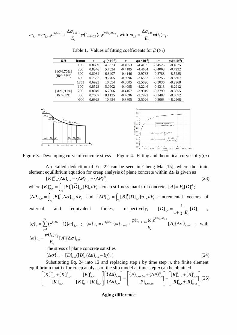
Shown in Fig. 4 is the time-relative developing curve of the concrete stress, with

creep considered from t0. Noting Δtn=tn-tn-1, Δσc,n=σc(tn)-σc(tn-1), Δσc,0=initial concrete stress,

Ec=elastic modulus of concrete, there are

0

c,0e cc

c c

d1( )

d

t

tt d

E E

(18)

0

c,0cr cc 0

c c

d( , )( ) ( , )

d

t

t

tt t t d

E E

(19)

where φ(t,τ)=creep coefficient; τ=age from the time when creep began. In the current Chinese

bridge design code [14], the creep coefficient is defined as

c( , ) ( ) ( )t t (20)

with

0.3

1c

H 1

( )( )

( )

t tt

t t

and

18

H

0 0

150 1 1.2 250 1500RH h

RH h

where φ(τ)=nominal creep coefficient; βc(t-τ)=development coefficient; βH=coefficient

relevant to RH and h; RH=annual average relative humidity; h=2A/u=theoretical thickness of

component; A=cross-sectional area of component; u=peripheral length of component in

contact with atmosphere; t1=1d; RH0=100%; h0=100mm.

For more convenience in programing, βc(t-τ) can be further fitted as

3

( )

c

1

( ) jq t

j

j

t c e

(21)

where the values of cj and qj (j=1,2,3) are listed in Tab. Shown in Fig. 4 are the fitting and

theoretical curves of φ(t,τ) when RH=55% and h=100mm, in which a high accuracy of the

fitting equation can be seen.

Combine Eq. 17, 18, 19, and 21 to obtain the creep strain increment within Δtn

cr cr cr

c, c c 1 c,( ) ( )n n n n n nt t (22)

where 3

,

1

( 1)j nq t

n j n

j

e

, 0.5

c

( , )n nn

t t

E

,

1 10.5c, 1

, , 1 1 0.5

c

( )j n j nq t q tn

j n j n n je t c eE

, with

c,0

,1 0

c

( )j jt cE

.

Table 1. Values of fitting coefficients for βc(t-τ)

RH h/mm c1 q1(×10-5) c2 q2(×10-3) c3 q3(×10-2)

[40%,70%]

(RH=55%)

100 0.8689 4.5373 -0.4053 -4.4105 -0.4525 -8.4025

200 0.8346 5.7034 -0.4185 -4.4664 -0.4068 -8.7232

300 0.8034 6.8497 -0.4146 -3.9733 -0.3788 -8.5285

600 0.7332 9.2705 -0.3996 -3.6582 -0.3256 -8.6367

≥833 0.6923 10.654 -0.3805 -3.5026 -0.3036 -8.2968

[70%,99%]

(RH=80%)

100 0.8523 5.0902 -0.4095 -4.2246 -0.4318 -8.2912

200 0.8049 6.7806 -0.4167 -3.9919 -0.3799 -8.6855

300 0.7667 8.1135 -0.4096 -3.7972 -0.3487 -8.6872

≥600 0.6923 10.654 -0.3805 -3.5026 -0.3063 -8.2968

0 t0 t1 t2 tn-1 tn tn+1…... t

σc

Δt1 Δt2 Δtn Δtn+1Δt0

Δσc,1

Δσc,2

Δσc,n+1

…...

Δσc,nΔσc,3

Δσc,n-1

tn-2

Δtn-1

Δσc,0

3( )

fitting

1

0.3

1theoretical

H 1

( , ) ( )

( )( , ) ( )

( )

jq t

j

j

t c e

t tt

t t

Figure 3. Developing curve of concrete stress Figure 4. Fitting and theoretical curves of φ(t,τ)

A detailed deduction of Eq. 22 can be seen in Cheng Ma [15], where the finite

element equilibrium equation for creep analysis of plane concrete within Δtn is given as

cr cr

cc, c, c, c,[ ] { } { } { }n n n nK u P P (23)

where c

cr T

cc, c c, c c[ ] [ ] [ ] [ ]n nV

K B D B dV =creep stiffness matrix of concrete; -1

c c[ ] [ ]A E D ;

c

T

c, c c, c{ } [ ] { }n nV

P B dV and

c

cr T

c, c c, c{ } [ ] [ ] { }n n nV

P B D dV =incremental vectors of

external and equivalent forces, respectively; c, c

c

1[ ] [ ]

1n

n

D DE

;

3

,

1

{ } ( 1){ }j nq t

n j n

j

e

;

1

1

0.5

1 0.5

, , 1 c, 1

c

( ){ } { } [ ]{ }

j n

j n

q t

q t n j

j n j n n

t c ee A

E

, with

0

,1 c,0

c

( ){ } [ ]{ }

j

j

t cA

E

.

The stress of plane concrete satisfies

c, c, c c,{ } [ ] ([ ] { } { } )n n n nD B u (24)

Substituting Eq. 24 into 12 and replacing step i by time step n, the finite element

equilibrium matrix for creep analysis of the slip model at time step n can be obtained

cr b b cr c ηc,cc, cc, cs, c, Δ c, cc, cc,

b s b s bs,sc, ss ss, s, Δ ss, bs,

{Δ }[ ] [ ] [ ] { } {Δ } [ ] [ ]

{Δ }[ ] [ ] [ ] { } [ ] +[ ]

nn n n n n n n n

nn n n n n n

uK K K P P R R

uK K K P R R

(25)

Aging difference

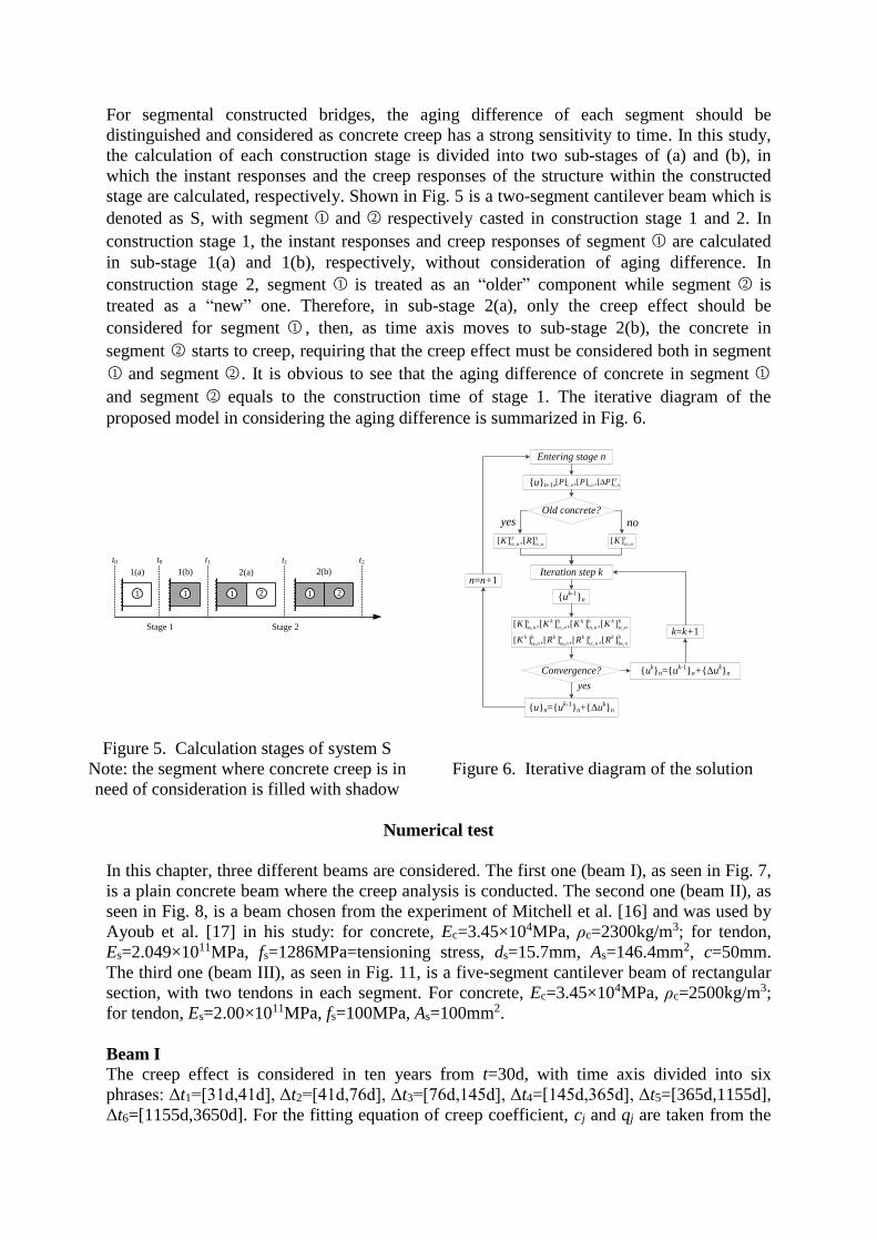
For segmental constructed bridges, the aging difference of each segment should be

distinguished and considered as concrete creep has a strong sensitivity to time. In this study,

the calculation of each construction stage is divided into two sub-stages of (a) and (b), in

which the instant responses and the creep responses of the structure within the constructed

stage are calculated, respectively. Shown in Fig. 5 is a two-segment cantilever beam which is

denoted as S, with segment ○1 and ○2 respectively casted in construction stage 1 and 2. In

construction stage 1, the instant responses and creep responses of segment ○1 are calculated

in sub-stage 1(a) and 1(b), respectively, without consideration of aging difference. In

construction stage 2, segment ○1 is treated as an “older” component while segment ○2 is

treated as a “new” one. Therefore, in sub-stage 2(a), only the creep effect should be

considered for segment ○1 , then, as time axis moves to sub-stage 2(b), the concrete in

segment ○2 starts to creep, requiring that the creep effect must be considered both in segment

○1 and segment ○2 . It is obvious to see that the aging difference of concrete in segment ○1

and segment ○2 equals to the construction time of stage 1. The iterative diagram of the

proposed model in considering the aging difference is summarized in Fig. 6.

t0 t1 t2

1 1 2

Stage 2

1 1 2

Stage 1

1(a) 1(b) 2(a) 2(b)

t0 t1

Entering stage n

Iteration step k

Convergence?

{u}n={uk-1}n+{Δuk}n

yes

{uk}n={uk-1}n+{Δuk}n

k=k+1

n=n+1

c

cc,[ ] nK

no

s b b b

ss, cc, cs, sc,

b s c b

ss, ss, cc, bs,

[ ] ,[ ] ,[ ] ,[ ]

[ ] ,[ ] ,[ ] ,[ ]

k k k

n n n n

k k k k

n n n n

K K K K

K R R R

{uk-1}n

{u}n-1,cr

c, s, c,[ ] ,[ ] ,[ ]n n nP P P

Old concrete?

cr η

cc, cc,[ ] ,[ ]n nK R

yes

Figure 5. Calculation stages of system S

Note: the segment where concrete creep is in

need of consideration is filled with shadow

Figure 6. Iterative diagram of the solution

Numerical test

In this chapter, three different beams are considered. The first one (beam I), as seen in Fig. 7,

is a plain concrete beam where the creep analysis is conducted. The second one (beam II), as

seen in Fig. 8, is a beam chosen from the experiment of Mitchell et al. [16] and was used by

Ayoub et al. [17] in his study: for concrete, Ec=3.45×104MPa, ρc=2300kg/m3; for tendon,

Es=2.049×1011MPa, fs=1286MPa=tensioning stress, ds=15.7mm, As=146.4mm2, c=50mm.

The third one (beam III), as seen in Fig. 11, is a five-segment cantilever beam of rectangular

section, with two tendons in each segment. For concrete, Ec=3.45×104MPa, ρc=2500kg/m3;

for tendon, Es=2.00×1011MPa, fs=100MPa, As=100mm2.

Beam I

The creep effect is considered in ten years from t=30d, with time axis divided into six

phrases: Δt1=[31d,41d], Δt2=[41d,76d], Δt3=[76d,145d], Δt4=[145d,365d], Δt5=[365d,1155d],

Δt6=[1155d,3650d]. For the fitting equation of creep coefficient, cj and qj are taken from the

first line of data in Tab. 1. To a determinant plane concrete structure where external forces

are applied at one time, the creep coefficient can be derived from the ratio of the creep

displacement/strain to the initial elastic displacement/strain. From Tab. 2, it can be seen that

the creep coefficient derived either by the calculated displacement or the calculated strain

displays a good agreement with the theoretical creep coefficient within each time step, and

concrete stress remains steady from beginning to the end, proving that the program has a high

accuracy in simulating the creep effect.

150 1502400 2400 2400

400

200

400

P=20kN P=20kN

Figure 7. Dimension and load conditions of beam I (Unit: mm)

Table 2. Calculation results of beam I

Step Age(d) Mid-span displacement(mm) Stain(×10-2) Stress(MPa)

Theoretical value of T C T/E T C T/E T C

Static 31 -14.3 0.0 0.00 -0.051 0.000 0.00 -17.7 0.0 0.00

Step1 41 -25.3 -11.0 0.77 -0.091 -0.040 0.77 -17.7 0.0 0.80

Step2 76 -34.9 -20.6 1.44 -0.126 -0.075 1.47 -17.7 0.0 1.48

Step3 145 -38.9 -24.6 1.72 -0.141 -0.090 1.76 -17.7 0.0 1.76

Step4 365 -45.4 -31.1 2.17 -0.164 -0.113 2.22 -17.7 0.0 2.22

Step5 1155 -50.3 -36.0 2.52 -0.181 -0.130 2.55 -17.7 0.0 2.56

Step6 3650 -54.7 -40.4 2.83 -0.198 -0.147 2.88 -17.7 0.0 2.88

Beam II

In this model, gradation loading proceeds in four steps. Load step 1: tension and anchorage of

tendon; Load steps 2~4: concentrated force P is applied step by step as per 0→10kN,

10→20kN, and 20→30kN at midspan. For the purpose of comparison, an ANSYS model is

established with tendon and concrete respectively simulated by element link 8 and solid 95 in

which full bonding is assumed to be existed between the two.

50 1815 1815 50

P

200

200

50

Figure 8. Dimensions and tendon layout of beam II (Unit: mm)

Lo

ad(k

N)

Ayoub(full bond)

Ayoub(bond-slip)

Procedure(bond-slip)

ANSYS(full bond)

Figure 9. Developing curves of midspan

displacements

Figure 10. Distribution of permanent stress and

prestress loss along the beam after anchorage

The load-displacement responses calculated by the proposed model, ANSYS model

and Ayoub’s model are shown in Fig. 9. Obviously, the development trends of the four

curves are consistent. The load-displacement response obtained by the proposed model draws

close to that by ANSYS model, for the element form and the mesh layout of them are the

same. Since the proposed model puts tendon slip into consideration, and ANSYS model

assumes full bond existing between tendon and concrete, the overall structural stiffness

calculated by the proposed model will be smaller than that by ANSYS, and therefore, the

midspan displacement calculated by the proposed model will be large than that by ANSYS

under the same loading level, which is also provided in Fig.9. Because of the differences in

element form, mesh layout and load processing, the calculation result of Ayoub’s model is

not that close to that of the proposed model although it considers tendon slip. The maximum

discrepancy between Ayoub’s model and the proposed model reaches as high as 18% at the

end of load step 1. Fig. 10 shows the distributions of permanent stress and prestress loss

along the beam after anchorage. The prestress loss mounts to the maximum at the end of

beam, reaching 105MPa, 8% of the tensioning stress, and attenuates towards midspan,

arriving at a stable level of 46MPa. On the contrary, the permanent stress mounts to the

maximum t midspan while slacks off at the end of beam, showing a transfer length, as what

Ayoub stated in his study.

Beam III

1 2 3 4 5

2000 2000 2000 20002000 1000

1000

Figure 11. Dimensions and tendon layout of beam III (Unit: mm)

In the process of cantilever construction, the control of the elevation is of great importance to

the final bridge line. As shown in Fig.11, although the dimensions of segment ○1 ~○5 are the

same, their stiffness and load contributions to the overall structure are still different for the

influence of concrete creep and aging differences. In Fig. 12 is shown the final construct line

when segment ○5 is finished. In the figure, the final displacement of the beam when creep is

considered is quite different from that when creep is not considered, indicating that the

concrete creep has a significant impact on bridge line of the construction stage. Fig. 13 shows

the tendon slippage along the beam. Obviously, the tendon slippage when creep is considered

is much larger than that when it is not, explaining that the concrete creep aggravates the

interaction between tendon and concrete, and thus further weakens the overall stiffness of the

structure.

Figure 12. Final displacements of beam III Figure 13. Tendon slippage along the beam

Conclusions

This study presents a spatial slip model for PC bridges, with concrete, tendon and interface of

the two simulated by 20-node solid element, 2-node truss element, and 4-node non-thickness

bond element, respectively. This model takes tendon slip into consideration with allowing

tendon to go through concrete in any patterns, which makes an improvement on the

traditional embedded and separated model. The finite element equilibrium equation of the

model is deduced and a modified Newton-Raphson iteration algorithm is adopted within the

solution of the equilibrium equations so that the stiffness and load matrices of the model can

be updated easily. Though numerical studies of three different beams, the accuracy of the slip

model is verified, where a distinguish difference between the responses whenever creep

effect is considered is easy to see, showing that concrete creep as well as aging difference has

a strong impact on the structure.

References

1. Aalami BO. Structural modeling of posttensioned members. J. Struct. Eng. 2000; 126(2): 157-162.

2. Shen JM., Wang CZ, Jiang JJ. Finite element analysis on reinforced concrete and the ultimate

analysis on slab and shell. Tsinghua University Press, Beijing, 1993.

3. Kang YJ. Nonlinear geometric, material, and time-dependent analysis of reinforced and prestressed

concrete frames. PhD thesis, University of California, Berkeley, Calif., 1977.

4. Van Zyl SF., Scordelis AC. Analysis of curved, prestressed, segmental bridges. Journal of the

Structural Division 1979; 105(11): 2399-2417.

5. Van Greunen J, Scordelis AC. Nonlinear analysis of prestressed concrete slabs. J. Struct. Eng. 1983;

109(7): 1742-1760.

6. Mari AR. Nonlinear geometric, material and time dependent analysis of three-dimensional

reinforced and prestressed concrete frames. Report. No. 84-12, SESM, University of California, Berkeley,

Calif., 1984.

7. Roca P, Mari AR. Nonlinear geometric and material analysis of prestressed concrete general shell

structures. Computers and Structures 1993; 46(5): 905-916.

8. Cruz PJS, Mari AR, Roca P. Nonlinear time-dependent analysis of segmentally constructed structures.

J. Struct. Eng. 1998; 124(3): 278-287.

9. Wu XH, Otani S, Shiohara H. Tendon model for nonlinear analysis of prestressed concrete structures.

J. Struct. Eng. 2001; 127(4): 398-405.

10. Zienkiewicz OC, Watson M, King IP. A numerical method of visco-elastic stress analysis.

International Journal of Mechanical Sciences 1968; 10(10): 807-827.

11. Zhu BF. The finite element method theory and applications. China Water Power Press, Beijing, 1998.

12. Long YC, Zhang CH, Zhou YD. Embedded slip model for analyzing reinforced concrete structures.

Engineering Mechanics 2007; S(1): 41-43.

13. Eligehausen R, Popov EP, Bertero VV. Local bond stress-slip relationships of deformed bars under

generalized excitations. Report EERC 83~23, Earthquake Engineering Research Center, University of

California, Berkeley, Calif., 1983.

14. Ministry of Communication of the People’s Republic of China. Code for design of highway

reinforced concrete bridges and culverts. China Communications Press, Beijing, 2004.

15. Ma C, Chen WZ. Numerical simulation of coupling time-varying effect of prestress and creep of PC

bridge. Bridge Construction 2013; 43(3): 77-82.

16. Mitchell D, Cook WD, Khan AA, Tham T. Influence of high strength concrete on transfer and

development length of pretensioning strand. PCI Journal 1993; 14(4): 62-74.

17. Ayoub A, Filippou FC. Finite-element model for pretensioned prestressed concrete girders. J. Struct.

Eng. 2010; 136(4): 401-409.