spatially explicit load enrichment calculation tool (select
TRANSCRIPT

1
Spatially Explicit Load Enrichment Calculation Tool (SELECT) and Load
Duration Curve (LDC) Analysis:Little Brazos River Tributaries Bacteria
Assessment Project
R. Karthikeyan, Ph.D.Biological and Agricultural Engineering
Texas A&M University, AgriLife [email protected]
979.845.7951
10/14/2008
2
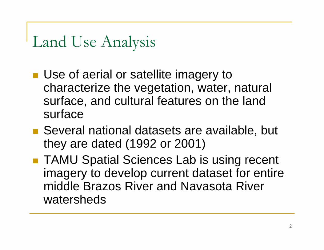
Land Use Analysis
Use of aerial or satellite imagery to characterize the vegetation, water, natural surface, and cultural features on the land surfaceSeveral national datasets are available, but they are dated (1992 or 2001)TAMU Spatial Sciences Lab is using recent imagery to develop current dataset for entire middle Brazos River and Navasota River watersheds
3
Spatially Explicit Load Enrichment Calculation Tool(SELECT)

4
Purpose of SELECTSpatially explicit analysis of LULC, animals in watershed, etc. to assess/determine potential sources of bacteria
http://www.awag.org/Education/Watershed_diagram.jpg
5
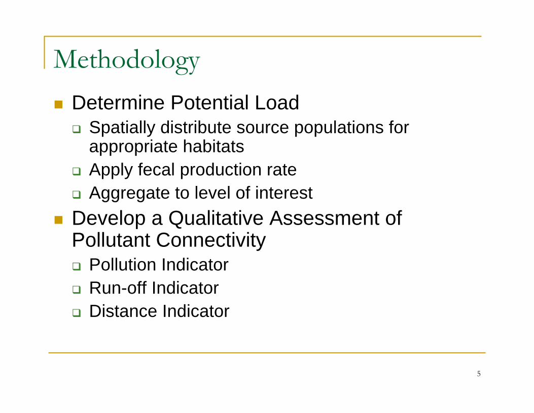
MethodologyDetermine Potential Load
Spatially distribute source populations for appropriate habitatsApply fecal production rateAggregate to level of interest
Develop a Qualitative Assessment of Pollutant Connectivity
Pollution IndicatorRun-off IndicatorDistance Indicator
6
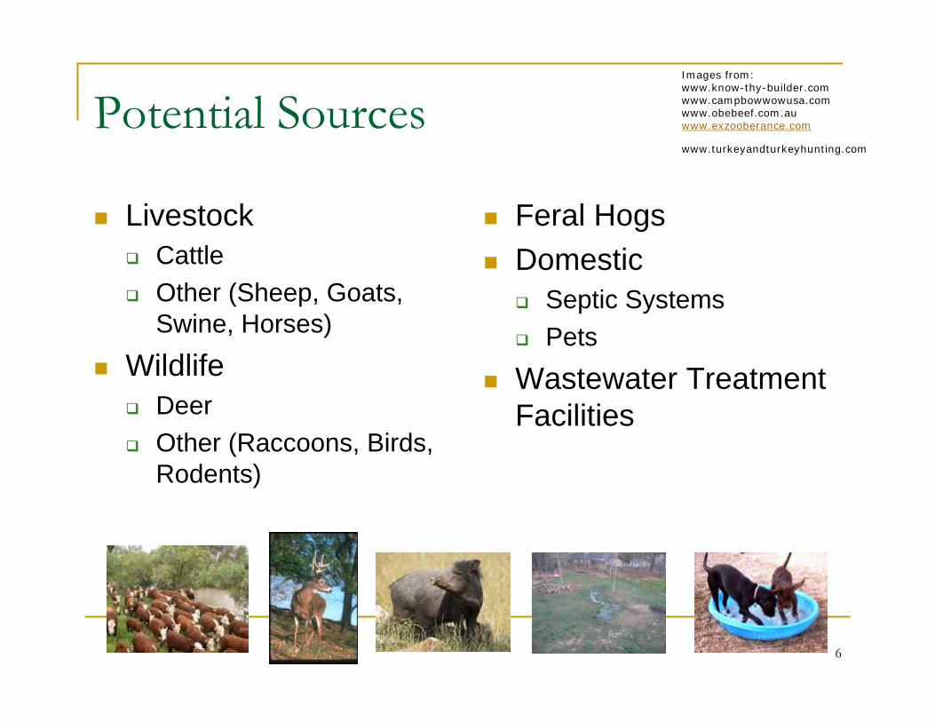
Images from:www.know-thy-builder.com www.campbowwowusa.com www.obebeef.com.au www.exzooberance.com
www.turkeyandturkeyhunting.com
Potential Sources
LivestockCattleOther (Sheep, Goats, Swine, Horses)
WildlifeDeerOther (Raccoons, Birds, Rodents)
Feral HogsDomestic
Septic SystemsPets
Wastewater Treatment Facilities
7
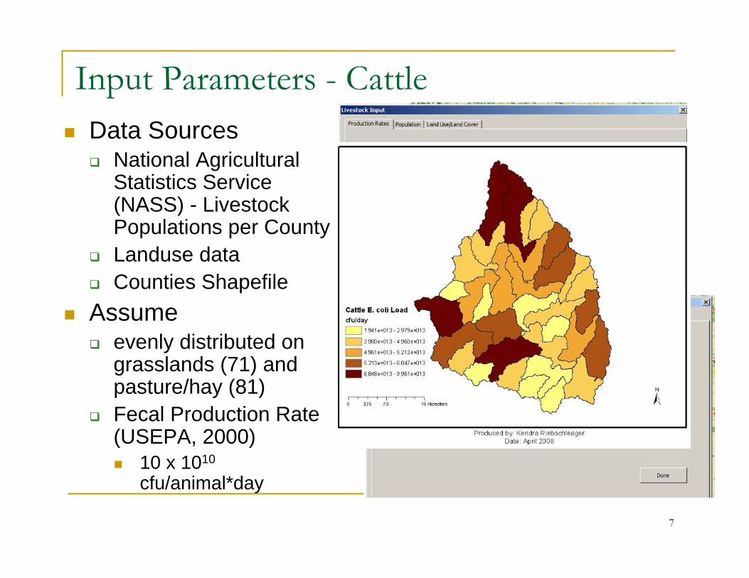
Input Parameters - CattleData Sources
National Agricultural Statistics Service (NASS) - Livestock Populations per CountyLanduse dataCounties Shapefile
Assume evenly distributed on grasslands (71) and pasture/hay (81)Fecal Production Rate (USEPA, 2000)
10 x 1010
cfu/animal*day

8
Total Potential E. coli Load

9
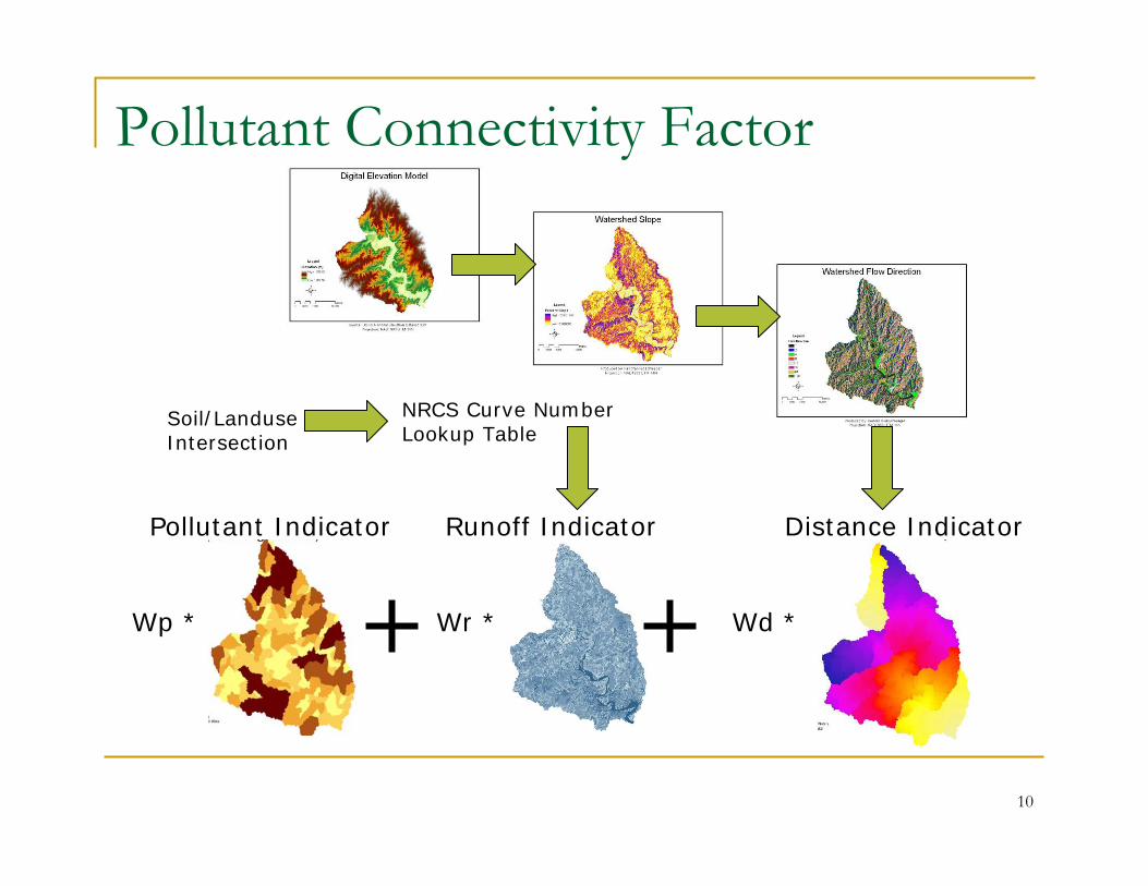
Pollutant Connectivity Factor
Contribution of Contaminant based onTotal pollutant loadingFate and Transport driven by
runofftravel distance
Growth and decay
Estimate influence of driving forces using weighted overlay
10
Pollutant Connectivity Factor
Pollutant Indicator
Wp * Wr *
Runoff Indicator
Wd *
Distance Indicator
Soil/Landuse Intersection
NRCS Curve Number Lookup Table

11
Load Duration Curve (LDC) Analysis
12
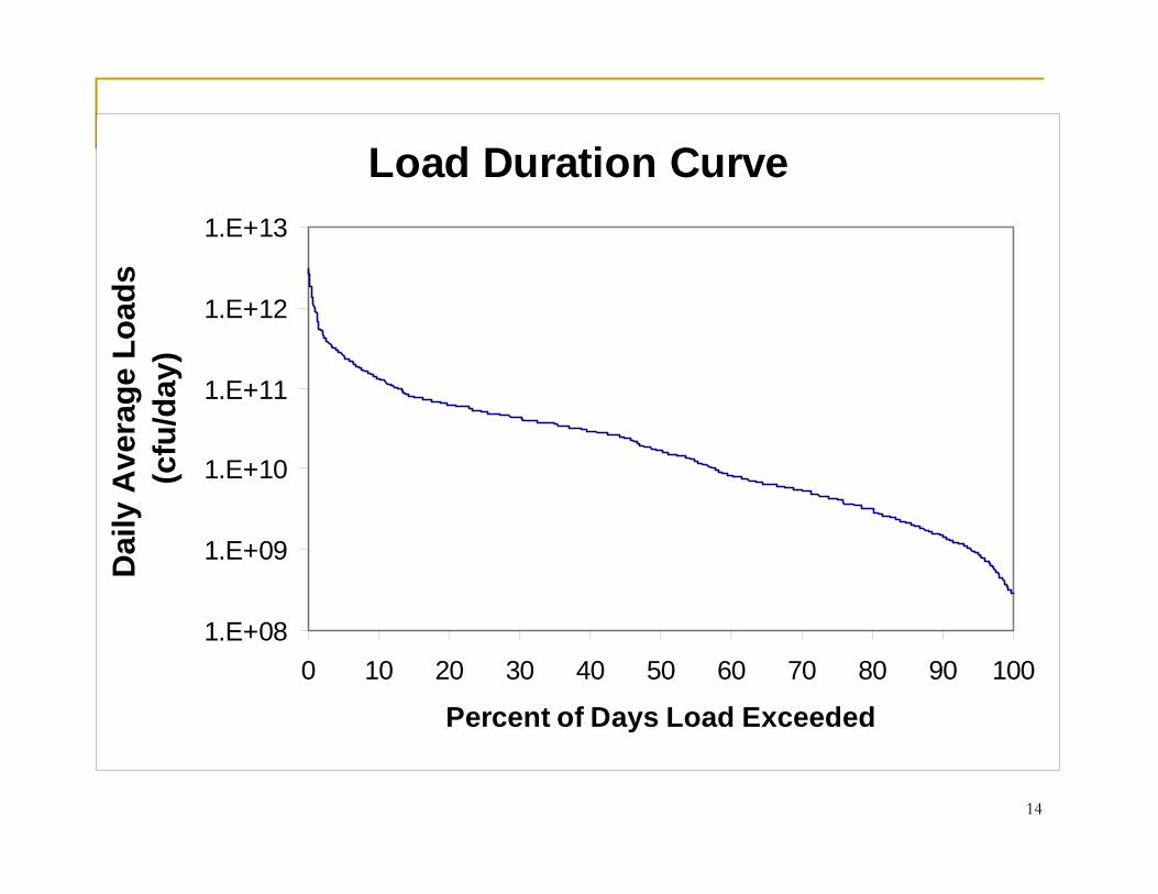
What is an LDC?
Graphical representation of streamflow and pollutant loadingsReal data can be compared to the stream’s maximum load to indicate reductions neededCan help to identify the type of pollutant load
13
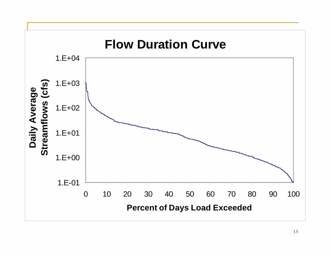
Flow Duration Curve
1.E-01
1.E+00
1.E+01
1.E+02
1.E+03
1.E+04
0 10 20 30 40 50 60 70 80 90 100
Percent of Days Load Exceeded
Dai
ly A
vera
ge
Stre
amflo
ws
(cfs
)
14
Load Duration Curve
1.E+08
1.E+09
1.E+10
1.E+11
1.E+12
1.E+13
0 10 20 30 40 50 60 70 80 90 100
Percent of Days Load Exceeded
Dai
ly A
vera
ge L
oads
(c
fu/d
ay)
15
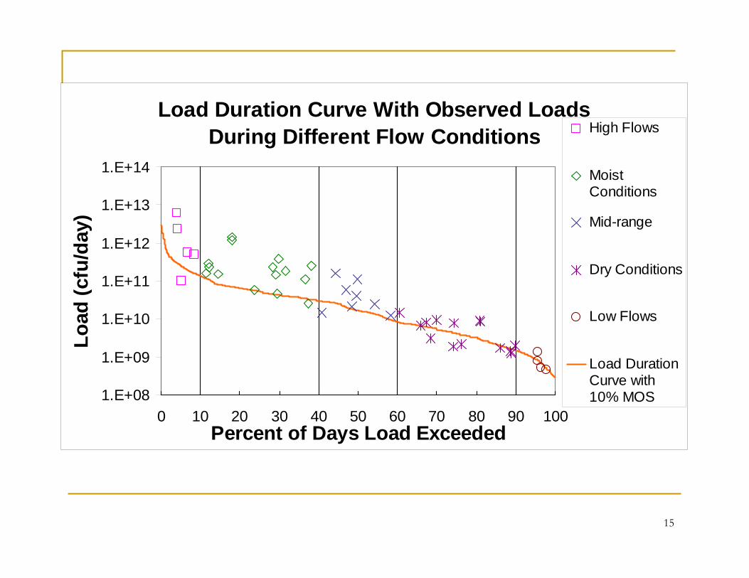
Load Duration Curve With Observed Loads During Different Flow Conditions
1.E+08
1.E+09
1.E+10
1.E+11
1.E+12
1.E+13
1.E+14
0 10 20 30 40 50 60 70 80 90 100Percent of Days Load Exceeded
Load
(cfu
/day
)
High Flows
MoistConditions
Mid-range
Dry Conditions
Low Flows
Load DurationCurve with10% MOS
16
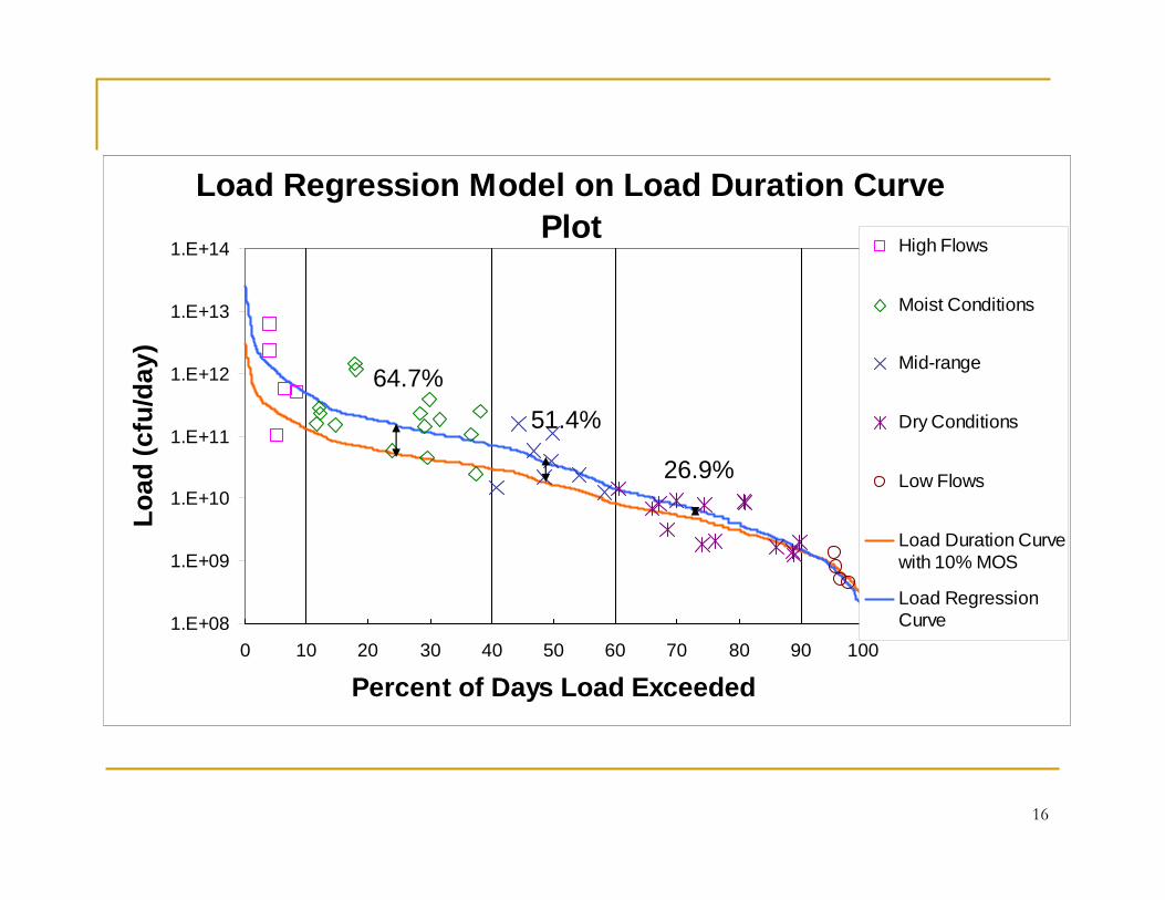
Load Regression Model on Load Duration Curve Plot
1.E+08
1.E+09
1.E+10
1.E+11
1.E+12
1.E+13
1.E+14
0 10 20 30 40 50 60 70 80 90 100
Percent of Days Load Exceeded
Load
(cfu
/day
)
High Flows
Moist Conditions
Mid-range
Dry Conditions
Low Flows
Load Duration Curvewith 10% MOS
Load RegressionCurve
64.7%
51.4%
26.9%
17
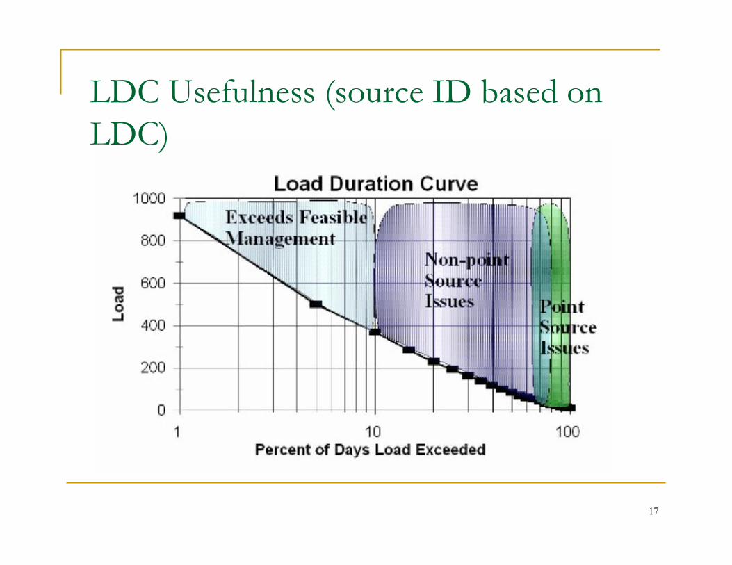
LDC Usefulness (source ID based on LDC)
18
Next Steps for Modeling
Next meeting is sanitary survey design, will have GIS work significantly completed (Nov or Dec 2008)
Meeting after that will show LDCs based on historical-only data and have model input questions for stakeholders (Dec 2008 or Jan 2009)
Meeting after that will show progress on SELECT (May 2009)

19
Questions?