spatially growing waves, intermittency, and convective chaos in an open-flow system

Physica 25D (1987) 233-260 North-Holland, Amsterdam

SPATIALLY GROWING WAVES, INTERMITTENCY, AND CONVECTIVE CHAOS IN AN OPEN-FLOW SYSTEM

Robert J. DEISSLER* Center for Nonlinear Studies, MS B258, Los Alamos National Laboratory, Los Alamos, New Mexico 87545, USA

Received 19 February 1986 Revised manuscript received 2 July 1986

Many flows in nature are "open flows" (e.g. fluid flow in a pipe). Here we study a model open-flow system: the time-dependent generalized Ginzburg-Landau equation under conditions when it is convectively (i.e. spatially) unstable. This equation is a partial differential equation which results from a reduction of the fluid equations of motion for a number of fluid systems. In the presence of low-level external noise, this system exhibits a selective spatial amplification of noise resulting in spatially growing waves. These waves in turn result in the formation of a dynamic structure. Three distinct spatial regions are found: 1) A linear region in which spatially growing waves are formed; 2) a transition region characterized by the transition from the spatially growing wave frequencies of the linear region to the turbulent frequencies of the fully developed region; and 3) a fully developed region in which the nonlinear dynamics dominates. In the transition region, the microscopic noise plays an important role in the macroscopic dynamics of the system. In particular, the external noise initiates the transition to turbulence and is responsible for the intermittent turbulent behavior observed in the transition region. Power spectra and correlation functions are calculated and analytical expressions are derived for these quantities in the linear region. Similarities between this system and fluid systems are discussed. Also, a few analytical results for coupled-map lattices are derived.

1. Introduction

Although much has been learned about turbulent fluid flow since Reynolds' classic 1883 experiment on turbulent flow in a pipe [1], turbulent fluid flow is still not well understood. This lack of understanding is due to the complexity of the equations of motion for fluid flow, the Navier- Stokes equations. In hopes of gaining a better understanding of turbulent flow, approximations are sometimes made to reduce the fluid equations (i.e. the continuity equations, the Navier-Stokes equations, and, for heat-convection systems, the energy equation) to a simpler set of equations. These reductions are more tractable for study than the original fluid equations while hopefully pre- serving the essential features under study. For

*Also at: Physics Department, 307 Nat Sci II, University of California at Santa Cruz, Santa Cruz, CA 95064, USA.

,Present and mailing address: National Center for Atmo- spheric Research, P. O. Box 3000, Boulder, CO 80307, USA.

incompressible fluid flow the Navier-Stokes equations in tensor notation are

3u, bu~ 3p 3 t + uj,--3xj - p V 2 u i = 3 x i '

where u i are the components of the velocity, p is the kinematic pressure (i.e. the pressure divided by the density), and u is the kinematic viscosity. The continuity equation is O u J O x i -- O.

One reduction of the fluid equations is the well-known Lorenz system [2]. This system consists of three coupled nonlinear ordinary differential equations which result from a truncation of a modal expansion of the fluid equations for a heat-convection system. Although the Lorenz system is extremely simple, much insight has been gained about the behavior of the more complex fluid systems. In particular the Lorenz system exhibits deterministic chaos-random behavior generated directly by the equations of motion-

0167-2789/87/$03.50 © Elsevier Science Publishers B.V. (North-Holland Physics Publishing Division)

234 R.J. Deissler / Convective ehaos in an open-flow system

which is believed to be an essential feature of fluid turbulence.

An important feature of fluids is the existence of complex spatial structure (e.g. irregular behavior in space), a feature which the simple Lorenz system is incapable of modeling. Therefore, to model some of the more complex behavior associated with spatial structure, a different reduction of the fluid equations is needed. One such reduction is the time-dependent generalized Ginzburg- Landau equation

o-7 = vg- - + - c1¢12¢, (1) ~X 2

where the dependent variable qJ (x, t) is in general complex; a, b, and c are constants which are in general complex; vg is the group velocity; and b r > 0. Real and imaginary parts of quantities are subscripted with r and i, respectively, or denoted by Re and Im, respectively. This equation results from expanding the variables of interest in powers of R - R c, where the control parameter R is near the critical value Re. The control parameter may be, for example, the Reynolds number, the Taylor number (Taylor-Couette flow), or the Rayleigh number (Rayleigh-B6nard convection).

To give the reader an indication of the meaning of ~ in eq. (1) for a physical system, we note that for two-dimensional plane Poiseuille flow (flow between two parallel planes) the stream function to first order in ( = ~/[R - Re[ is [5]

((x ,y , t )

= y - y 3 / 3 + 2( Re [+ (X, ~') q~(Y) ei(k . . . . t)].

Here x and y are the spatial coordinates parallel and perpendicular to the planes, respectively; X = cx and ~- = (2t are slowly varying space and time variables; k c and ~0 c are the wavenumber and frequency corresponding to the critical Reynolds number Rc; y-y3/3 is the unperturbed laminar state; and ~ ( y ) is a function of y only and is determined by a differential equation in y. In eq. (1), a and c are of the order of e2; and vg and b

are of the order of e °. The velocity components parallel and perpendicular to the planes, respectively, are u = - ( 0 ~ ) / ( 0 y ) and v=(O~)/(Ox). Since +(X, T) is the slowly varying amplitude of a plane wave, eq. (1) is often referred to as an amplitude equation. For more details the reader is referred to refs. 3-6.

Being a partial differential equation eq. (1) is capable of exhibiting complex spatial structure. The term with the first-order spatial derivative is a convective term which causes a "mean flow". This convective term may be unfamiliar since vg = 0 for many of the systems which can be reduced to eq. (1). Also, even for systems with vg ¢ 0, eq. (1) is often written in a frame of reference moving at velocity vg which means the convective term will not appear. Some fluid systems which have been reduced to eq. (1) are Rayleigh-Brnard convection (% = 0) [3], Taylor-Couette flow (% -- 0) [4], plane Poiseuille flow (v g4: 0) [5], and wind-induced water waves (% 4: 0) [6]. Depending on parameter values and boundary conditions eq. (1) can model either a "closed-flow" or an "open-flow" system [7]. Eq. (1) is very easy to solve numerically compared with the original fluid equations and, as we shall see, shares many of the features of real fluid systems. Studying this equation can therefore provide insights into the workings of real fluid systems and indicate directions of study for numerical and experimental studies of turbulent fluid flow.

The first-two fluid systems mentioned above (i.e. Rayleigh-Brnard convection and Taylor- Couette flow) are examples of closed-flow systems. In a closed-flow system the flow "closes back on itself" and no fluid enters or leaves the system under consideration. For example, in Taylor- Couette flow the system consists of the fluid within the region enclosed by the concentric cylinders and the end plates; and in Rayleigh-Brnard convection the system consists of the fluid within a box across which there is a temperature difference. The fluid constantly recirculates within these regions. Therefore, any small growing perturbation will be recirculated in the flow and eventually

R.J. Deissler / Convective chaos in an open-flow system 235

contaminate the entire flow. With vg = 0 eq. (1) models a closed-flow system (or a portion of an open-flow system in a moving frame of reference). Also, with periodic boundary conditions eq. (1) models a closed-flow system.

The second-two fluid systems mentioned above (i.e. plane Poiseuille flow and wind-induced water waves) are examples of open-flow systems. In order for these to be open-flow systems the boundary conditions cannot be periodic or else the systems will be closed flows. Other examples of open-flow systems are fluid flow over a flat plate, fluid flow in a pipe, fluid flow in a channel, jets, and smoke rising from a cigarette. In contrast to a closed-flow system, an open-flow system is open to mass flux and fluid enters and leaves the system under consideration. For example, in pipe flow the system consists of the fluid within the pipe; and in flat- plate flow the system consists of the fluid above the plate. The fluid enters one end and leaves at the opposite end. A typical characteristic of open- flow systems (in contrast to closed flows) is the spatial development of the flow. For example, in flat-plate flow there are distinct spatial regions starting from the leading edge of the plate: a laminar region, spatially growing waves, nonlinear breakdown resulting in turbulent spots, and fully developed turbulence. Also, in contrast to closed flows, instabilities are typically convective in nature for open flows*. For example, in flat-plate flow a small localized growing perturbation will be convected downstream with the flow [28]. With vg greater than some critical velocity so that the state ~p = 0 is convectively unstable, eq. (1)(with nonperiodic boundary conditions) models an open- flow system* *.

Prior to the work described in ref. 8, the Ginzburg-Landau equation had only been studied for Vg = 0 [9-13]. Therefore those studies [9-13]

*One exception to this is shear flows where the flow may be either absolutely unstable or convectively unstable [30].

**The converse, however, is not necessarily true since some open-flow fluid systems (e.g. shear flows [30]) can have laminar solutions which are absolutely unstable. Also, all amplitude equations are not of the form of eq. (1).

modeled a closed-flow system (or a portion of an open-flow system in a moving flame of reference). However as was shown in ref. 8, the behavior of eq. (1) [in the stationary (i.e. laboratory) flame of reference] is very different under conditions when the system is convectively (i.e. spatially) unstable. When a system is convectively unstable, a small perturbation will eventually damp at any given stationary point but a moving frame of reference may be found in which the perturbation is growing. In particular, under such conditions, low levels of external noise can be selectively and spatially amplified forming spatially growing waves, which saturate at some spatial point forming a dynamic structure. Typically there are three distinct spatial regions: 1) A linear region in which spatially growing waves are formed; 2) a transition region in which nonlinear effects come into play (this region may exhibit intermittent turbulent behavior in which the external noise plays a crucial role); 3) a "ful ly developed turbulent" region in which the nonlinear dynamics dominates. These types of behavior are typical for experimental open-flow systems.

Some points of ref. 8 were: 1) Under conditions when the system was convectively unstable, the external noise (or other perturbation) was essential for the formation of a structure - no noise ~ no structure. 2) The external microscopic noise played an important role in the macroscopic dynamics of the system (e.g. the intermittency) [14]. 3) Since in the deterministic limit (i.e. no noise) the state of the system is at rest (i.e. ~ = 0), the chaotic behavior is not associated with a strange attractor. 4) Since low levels of external noise can play an important role in the macroscopic dynamics of systems, it can be crucial to include external noise in the modeling of some systems.

Although the convectively unstable Ginzburg- Landau equation is an ideal model for an open- flow system in the sense that it results from a reduction of the fluid equations, the first simple model for an open-flow system was introduced in ref. 16. There the author studied a system of points coupled with logistic maps. Although this

236 R.J. Deissler / Convective chaos in an open-flow system

system does not result from a reduction of the fluid equations it nonetheless exhibits behavior characteristic of many open-flow systems (e.g. a spatial amplification of external noise resulting in a dynamic structure). Also, the notion of noise- sustained structure was introduced in this reference and the study of this system originally lead the author in a search for a more realistic (but still simple) model for an open-flow system (i.e. the Ginzburg-Landau equation). Although the major- ity of the discussion will be on the Ginzburg- Landau equation since it's behavior corresponds more closely to real fluid systems, we still include an appendix on convectively unstable coupled-map lattices in order to present a few analytic results that the author derived since ref. 16.

In sections 2 and 3 of this paper we discuss linear stability and noise-sustained structure. Much of the content of these two sections may be found in ref. 8. In sections 4 and 5 the linear and transition regions are discussed. In particular we calculate power spectra and correlation functions and derive analytical expressions for the power spectra and correlation functions in the linear region. Also we look in more detail at the intermittency which occurs in the transition region. In section 6 we discuss the fully developed region and also discuss and somewhat extend some of the ideas and results of ref. 15, where a measure of chaos for the fully developed region was given. In section 7 we discuss features that the Ginzburg- Landau system has in common with actual fluid systems and suggest possible avenues of research for numerical and experimental open-flow fluid systems. In appendix A we discuss the discrete Fourier transform and derive some relationships. In appendix B we discuss a few generalizations of eq. (1). In appendix C we present a few analytic results for convectively unstable coupled-map lattices.

' t=0 / ~ ABSOLUTELY

. ~ t '>0 UNSTABLE

t = 0 ~ \ ABSOLUTELY

t > 0 STABLE

t = 0 / A \ CONVECTIVELY

~ 0 UNSTABLE

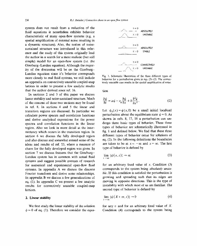
Fig. 1. Schematic illustration of the three different types of behavior for a perturbation given in eqs. (3)-(5). The convectively unstable case results in the spatial amplification of noise.

tion

a¢=a~- a¢ ba2+ (2) Ot vg~x q- OX 2"

Let ~k0(x)=+(x ,0 ) be a small initial localized perturbation about the equilibrium state ~k = 0. As shown in refs. 8, 17, 18 a perturbation can un- dergo three basic types of behavior. These three types of behavior are schematically illustrated in fig. 1 and defined below. We find that these three different types of behavior occur for solutions of eq. (2). In the following definitions the boundaries are taken to be at x = - o 0 and x = oo. The first type of behavior is defined by

lim I¢ (x , t ) l ~ oo (3)

for an arbitrary fixed value of x. Condition (3) corresponds to the system being absolutely unstable. If this condition is satisfied the perturbation is growing and spreading such that its edges are moving in opposite directions. This is the type of instability with which most of us are familiar. The second type of behavior is defined by

2. Linear stability lim I~(X+vt, t ) [~O (4) t ~ O O

We first study the linear stability of the solution = 0 of eq. (1). Therefore we consider the equa-

for any v and for an arbitrary fixed value of X. Condition (4) corresponds to the system being


absolutely stable. If this condition is satisfied the perturbation is damped in any frame of reference. The third type of behavior is defined by

lim [ ~ p ( x , t ) [ ~ 0 and lim [~(X+vt, t ) l ~ o o t ---* Or3 t---~ oC

(5)

of eq. (2) is absolutely unstable if

v~br a t - 4[b[-----~> 0; (7)

absolutely stable if

a r < 0 ; ( 8 )

for some v and for arbitrary fixed values of x and X, respectively. Condition (5) corresponds to the system being convectively unstable (i.e. spatially unstable). If this condition is satisfied the perturbation is damped (as t ~ oo) at any given stationary point, but a moving frame of reference may be found in which the perturbation is growing. Therefore, even though the perturbation is growing and spreading, the perturbation is moving at a sufficiently large velocity such that both edges of the perturbation are moving in the same direction, thus allowing the system behind the perturbation to return to its undisturbed state. This is the type of instability in which we are mainly interested in this paper since it will result, as also noted by ref. 18, in the amplification of noise. For the cases considered in this paper the "any v" of condition (4) and the "some v" of condition (5) may be replaced by "v = %", where vg is the group velocity of the perturbation.

Taking the boundaries at x--- - o o and x = oo, the subsequent evolution of the perturbation for the linear eq. (2) is given by

__ e at f o o ) 2 ( ~ r b t ) l / 2 _ oo d x ' @ 0 ( x '

e - ( X - V t - X ' ) 2 / ( 4 b t ) .

(6)

This comes from simply writing ~p as a Fourier integral and performing the integral over wave number (see eq. (32) in appendix B). Applying the conditions (3)-(5) to eq. (6), and noting that it is easier to take the limit before taking the magnitude, we find that the equilibrium solution ~ - - 0

and convectively unstable if

v2br < 0 and a r > 0 . (9) ar 41bl 2

The first part of condition (9) may be written as ]%1 > 21bl(ar/br) 1/2 which simply says that the magnitude of the group velocity of the perturbation must be greater than the magnitude of the velocity at which it spreads (i.e. speed of an edge relative to the co-moving frame). This critical velocity is the same as that given by the Dee-Langer marginal-stability condition [11, 19], which gives the velocity of a pattern front. Note that, since b r > 0, a r > 0 if condition (7) is satisfied and ar-vEbr/(41bl2)<O if condition (8) is satisfied. It may be instructive to note that for an initial Gaussian perturbation, ~b0(x ) = A e -~x2,

eat - a ( x - vt)2/(1 + 4abt) ~p(x, t) = A (1 +4abt) 1/2 e

The three types of behavior become particularly clear in examining this solution.

As noted in ref. 8, another method to determine whether or not a system (with a given set of nonperiodic boundary conditions) is convectively unstable is to first calculate the eigenvalues of the system with the given set of boundary conditions, and to then calculate the eigenvalues of the system with periodic boundary conditions imposed instead. If Re[?~g] < 0, where ~,g is the eigenvalue with the largest real part for the given set of boundary conditions, and Re[Xp] > 0 where ?% is the eigenvalue with the largest real part for the


system with periodic boundary conditions imposed instead, then the system will be convectively unstable. This follows from the fact that a spatially growing perturbation which would have otherwise traveled out through a boundary of a convectively unstable system, will be fed back through the other boundary if the boundary conditions are instead periodic. Note that Re[Xg] > 0 implies an absolute instability and that Re [X p] < 0 implies an absolute stability. It is assumed here that the dimensions of the system are large enough such that a perturbation can grow significantly before leaving the boundaries of the system.

3. Noise-sustained structure

As previously noted, eq. (1) with vg = 0 has been numerically studied by a number of researchers. If a r > 0 this system is absolutely unstable. If the equilibrium solution + = 0 is given a small (microscopic) local perturbation for a r > 0, the perturbation will grow with time eventually reaching macroscopic proportion. If c r > 0 the amplitude will saturate and thus the perturbation will grow to a finite size producing a structure, which will most likely be changing with time (i.e. dynamic). Periodic, quasi-periodic, and chaotic structures have been observed. The main point here is that a single perturbation is sufficient to produce a structure for all time.

In contrast, if vg is nonzero and sufficiently large, the perturbation and resultant structure will move spatially such that the structure will eventually leave the boundaries of the system. Thus the system will return to the equilibrium state. A single perturbation will therefore produce only a temporary structure. However if the system is con-

tinuously perturbed by microscopic fluctuations the system will be unable to return to the equilibrium state and a new state will be established which is sustained by the presence of the fluctuations. We refer to such a state as a noise-sustained state and the corresponding structure as a noise- sustained structure. We assume that the spatial

growth factor of the fluctuations and the length of the system are large enough such that the fluctuations will reach macroscopic proportion and produce a structure before they leave the boundaries of the system. From the previous discussion on linear stability it is clear that a necessary condition for noise-sustained structure is that the system is convectively unstable. For example, if vg is sufficiently large and small fluctuations are introduced into the left boundary, the fluctuations will grow spatially until nonlinear effects enter which will cause the fluctuations to saturate (assuming c r > 0), forming a structure.

We now show some numerical results. Second- order Runge-Kut ta is used in the time differencing and fourth-order differencing is used in the space differencing [20], except at the grid points adjacent to the boundaries where second-order differencing is used. The distance between spatial grid points is Ax = 0.3, and the time step is At = 0.01. The boundary conditions are }(0, t) = 0 and ~b"(L, t ) = 0 (to approximate an open boundary [45]), where a prime denotes a spatial derivative*. External noise is introduced into the left boundary by letting q~r(0, t) and qJi(0, t) equal (at each time step) random numbers uniformly distributed between - r and r. Introducing the noise in this fashion allows for some analytical results and does not change the qualitative behavior of the system from that of ref. 8 (where the noise was added to all grid points except the left boundary).** Cray single precision (14 digit accuracy) is used in the calculations. We start with the initial equilibrium state q~ = 0 and allow the system to evolve in the presence of this small amount of external noise to a state for which transients have settled down (i.e. to a statistically steady state).

Fig. 2 shows plots of the real and imaginary parts of ~ as a function of x for a given value of

*This boundary condition was chosen mainly for aesthetic reasons. Even if the right boundary is fixed, the behavior of the system changes only near that boundary.

**If other types of noise (e.g. Gaussian white noise) are used, the qualitative behavior of the system remains un- changed.

R.J, Deissler / Convective chaos in an open-flow system 239

50 100 150 2 0 0 2..50 ,.500 a X

'•J ' i ' I ' [ ' I ' 3 0 0 320 540 560 3 8 0 4 0 0 a

f

~ o

0 k 50 100 150 2 0 0 250 3 0 0 IL/

X

Fig. 2. Plots of tpr a n ~i as a function of x for a given t ( t = 200) after the system has reached a statistically steady state, a = 2, vg = 5.2, b r = 1.8, b i = - 1 , c r = 0 . 5 , c i = 1. Noise level = r = 10-7. The microscopic noise at the left boundary grows spatially to macroscopic proportion resulting in the observed structure. The spatial point at which the structure becomes irregular changes with time.

t. W e see tha t the f luc tua t ions at the left b o u n d a r y

g r o w spa t i a l ly to macroscop ic p r o p o r t i o n resu l t ing

in the o b s e r v e d s t ructure . The s t ruc ture in fig. 2 is

a n o i s e - s u s t a i n e d s tructure . I f the ex te rna l no i se is

r e m o v e d , the s t ruc ture moves ou t th rough the

f ight b o u n d a r y a n d the sys tem re tu rns to the s ta te

~k = 0 everywhere , except for some slight ( <

10 -1°° ) f l uc tua t i ons due to c o m p u t e r roundoff .

C o n d i t i o n (9) is satisfied since vg = 5.2 is greater

t h a n the cr i t ical veloci ty 2 [ b l ( a r / b r ) a/2 which

equa l s 4.341 for the p a r a m e t e r va lues of fig. 2. W e

see tha t there are d i s t inc t spat ia l reg ions as m e n -

t i o n e d in the i n t r o d u c t i o n . W e n o w s tudy each

r e g i o n separa te ly .

4. The linear region

m ,? o

3 0 0 b 320 340 360 3 8 0 4 0 0

f

. I v, - , I 300 320 340 360 380 400

c t

m o

lv\i! v v l l v l 300 d 320 340 360 380 400

T h e l i n e a r reg ion is tha t r eg ion where the

f l u c t u a t i o n s are smal l e n o u g h to be cons ide red

l inear . F r o m fig. 2 we see tha t this r eg ion ex tends

f r o m x - 0 to a b o u t x = 35. Fig. 3 shows plots of

Fig. 3. Plots of ~bf as a function of t for different values of x in the l i n e a r region, a = 2, vg = 5.2, b r = 1.8, b i = - 1, c r =

0.5, c i = l . a) x = 0 ; b) x = 3 ; c) x = 6 ; d) x=30. Thesignal becomes more regular for larger values of x as a result of the selective amplification of the noise introduced at x = 0. Note the change in vertical scale.


r as a function of t for various values of x in the linear region. We see that the noise at the left boundary (fig. 3a) is selectively amplified thus causing the time series to be more regular for larger values of x *

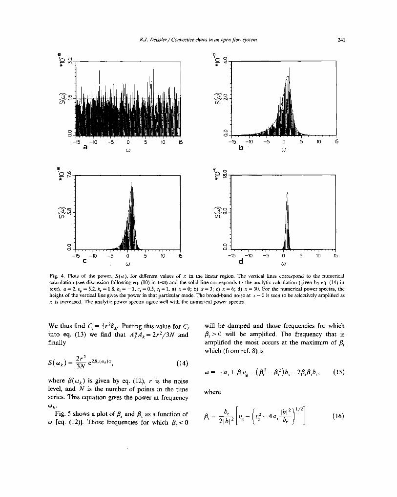
This selective amplification can be more clearly seen in fig. 4 (vertical lines) which shows the power spectra at the same values of x as those of fig. 3. Writing

~(x , t) ----- ~ Bk(X)e -i''kt, (10)

the power spectrum is defined by S(¢ok)= B~B k. Here ~0 k = 2~rk/T, where T is the length of the time series taken and the * denotes the complex conjugate. Fast Fourier transforms were used to calculate the spectra. The sampling rate was A t = 0.01 (equal to the time step in the numerical integration), and 61 averages were done (with 75% overlap). The number of points in each of the series that were averaged was N = 4096. The frequency resolution is therefore A~o = 2~r/(NAt) = 0.153 (equal to the separation between the vertical lines). The height of the vertical line gives the amount of power in that particular mode (at frequency ¢0k). With more averages the spectra would become smoother. As can be seen in fig. 4a the noise is a good approximation to white noise. For larger values of x the frequency band becomes more narrow which agrees with the behavior seen in fig. 3.

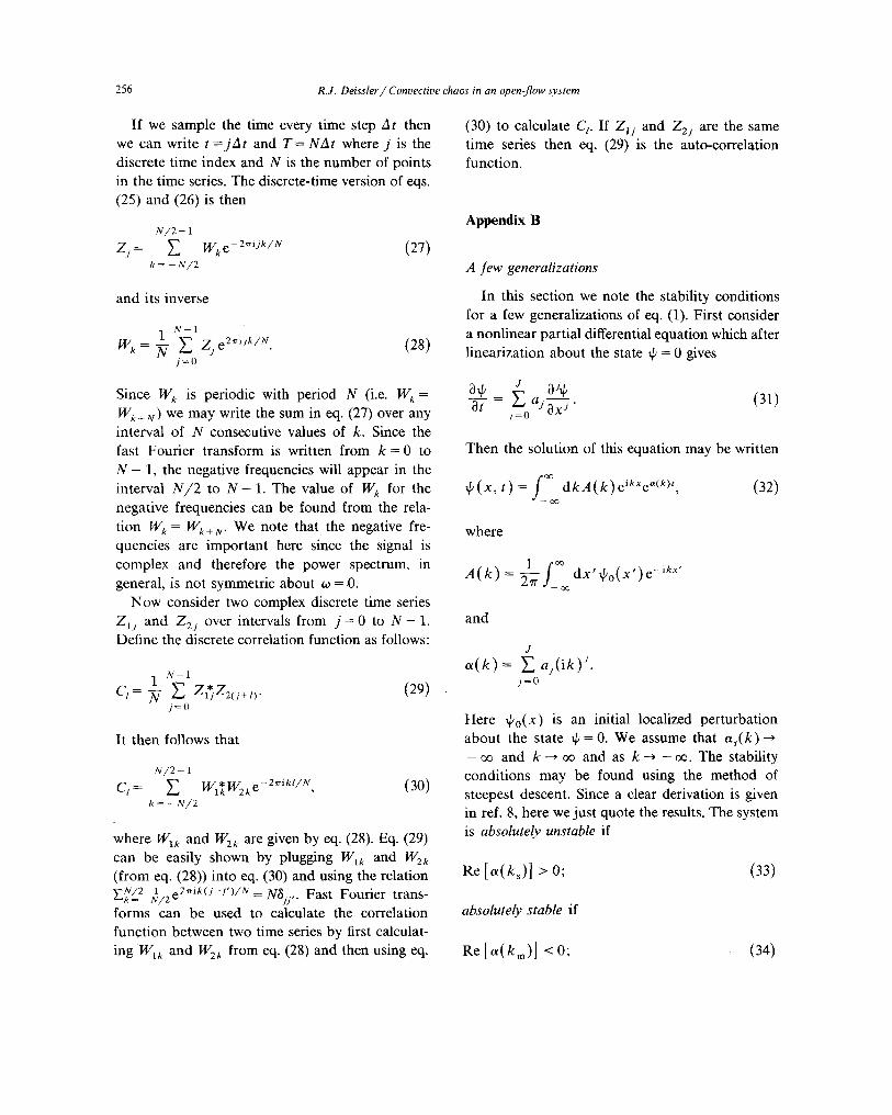
We can get an analytic expression for the power spectrum in the linear region in the following fashion. A solution of eq. (2) is

~ ( x , t ) = ~ Ake#~e i,~,t. (11) k= ao

- f l k b . Solving for flk gives -- iw k = a flkUg ..~ 2

Bk= --~[Vg-- ~Vg--4b(a+ i~Ok) ], (12)

where the principal value of the square root is taken (i.e. Re ( > 0) and it is assumed that vg is positive and that condition (9) is satisfied. Com- paring eq. (11) with eq. (10) we seen that the power spectrum is S k - ~ * ~ ,,2arkx

To determine AkA ~ we have q,(0, t ) = ors --i~kt

~ - ~ k = - ~ A k e which we approximate as qJjl~=0 S~N/2 1 A ~ iwk At j ,.,k=_U/2,~k~ where t=jAt and Wk=

2~rk/(Nat). We also have that the discrete auto- correlation function (see eqs. (29) and (30) in appendix A) is

I N 1 N / 2 - 1 C I = N E ~ ? ~ j + l = E d * d o-2¢rik l /N

j = 0 k = - N/2

(13)

At x = O, lpr and ¢i are random numbers. There- fore, assuming that the random numbers are uncorrelated and that N is sufficiently large so that the only significant contribution to C t occurs at l = 0 we have

1 N-1 c,= E +N0+

j=O

1 N--1 = N E [ ~ r j - - i ~ i j ] [ ~ r ( j + l ) - k - i ~ i ( j + l ) ]

j=0

1 N 1

j=O

Since the random numbers are uniformly distributed between - r and r the last expression can be evaluated in the limit as N ~ ~ as follows:

Putting this solution into eq. (2) we find that N-1 1 N-1 r2 N~I ( j ) 2

1 2 2 Z ~ r y = N " Z LPij= N-

j=0 j=0 j~0

*The amplitude of the signal in fig. 3b is less than that in fig. 3a as a result of the damping of the high frequencies over a small spatial region.

r2N(N- 1 ) ( 2 N - 1) r 2 = ~ - .

6N(N - 1) 2


' 0 ~. v - -

O3 cq-

O3

-15 c5

-10 - 5 0 5 10 15 -15 -10 - 5 0 5 10 15 a b b2

~O to , - - r < .It-

•,•0o U3

o. o

*

(/3

0 . . . . I . . . . I . . . . I ' ' I . . . . I . . . .

-15 -10 - 5 0 5 10 15 -15 -10 - 5 0 5 10 15 c d

Fig. 4. Plots of the power, S(oJ), for different values of x in the linear region. The vertical lines correspond to the numerical calculation (see discussion following eq. (10) in text) and the solid line corresponds to the analytic calculation (given by eq. (14) in text), a = 2, vg = 5.2, b r = 1.8, b i = - 1 , c r = 0.5, c i = 1. a) x = 0; b) x = 3; c) x = 6; d) x = 30. For the numerical power spectra, the height of the vertical line gives the power in that part icular mode. The broad-band noise at x = 0 is seen to be selectively amplified as x is increased. The analytic power spectra agree well with the numerical power spectra.

We thus find C, = ~ r 2 8 o l . Putting this value for C l into eq. (13) we find that AkAk= 2rE/3N and finally

s(to ) = * 3N ~ ( 1 4 )

where fl(tok) is given by eq. (12), r is the noise level, and N is the number of points in the time series. This equation gives the power at frequency Oak.

Fig. 5 shows a plot of fir and fli as a function of to [eq. (12)]. Those frequencies for which fir < 0

will be damped and those frequencies for which fir > 0 will be amplified. The frequency that is amplified the most occurs at the maximum of fir which (from ref. 8) is

to = _ ai +/~ iOg _ ( f12 _ fl2)b i _ 2flrflibr, (15)

where

br [ ( 2-4a Iblz]l/2] (16) fir = 2lb[ 2 % - vg r br ] J


tq. 0

~_? \

\ . \ T . . . . I . . . . [ . . . . [ . . . . I . . . . ] . . . .

-15 -10 -5 0 5 10 15 a

O

cJ

-20

-15 ' ' ' 1 . . . . I ' ' ' ' 1 . . . . I . . . . I . . . .

-10 -5 0 5 10 15

b w

Fig. 5. Plots of flr(~0) and ill(tO) as given by eq. (12). fir is the spatial growth factor and fli is the wavenumber. Only those frequencies such that fir > 0 will be amplified. The frequency that is most amplified corresponds to the maximum of fir-

and

_ [ t 4a Xj21 b, - ( 17 ) fli = 21bl 2 0 g r b, ] J"

Eqs. (16) and (17) give the spatial growth factor and the wavenumber corresponding to the frequency that is most amplified• Inserting the parameter values from the figures we find ~0 = 1.111 which agrees well with the frequencies seen in figs. 3d and 4d.

Fig. 4 (solid curve) shows plots of the power spectra from eq. (14). We see that the analytical

10 ~-

S t'-.

. . . . I ' ' ' ' ' ' ' ' I . . . .

-10 -5 0 5 10

a T

-10 0 10 20 50 40

b r

~ L J ( % •

(.9

O

*

O ,

-20

o~ C9

-10 0 10 20 30 40

C "7-

Fig. 6. Plots of the magnitude of the correlation function ( G ( r ) = I C ( r ) l ) between two different spatial points x 1 and x 2 in the linear region as a function of the lag time (see eq. (13) in text). The solid curve corresponds to the numerical calculation and the dashed curve corresponds to the analytic calculation (given by eq. (18) in text), a = 2, vg = 5.2, b r = 1.8, bi = - 1 , Cr =0 .5 , c i= 1. a) X l = 0 , x 2 = 3; b) xl = 0 , x2 = 30; c) x 1 = 3, x 2 = 30. The time series at some spatial point is seen to be correlated with the noise• The analytic expression agrees well with the numerical calculation.


power spectra agree well with the numerical power spectra.

Fig. 6 (solid curve) shows plots of the magnitude of the correlation function between two different spatial points (see appendix A). These were calculated by using fast Fourier transforms to first calculate the Fourier transforms at two different

spatial points x 1 and x 2 [i.e. Bk(Xl) and Bk(x2) in eq. (10)] and then calculating the inverse Four- ier transform of B~(xl)B~(x2) giving the correlation function. The number of points used in the transforms was 65536 and the sampling rate was again At = 0.01. As expected, we see that the time series at some point x is correlated with the noise at x = 0 with the maximum occurring at some delay ~-. This means that the irregularities (i.e. variations of amplitude, frequency, a n d / o r phase) in the time series at the point x is the direct result of the external noise.

We now get an analytical expression for the correlation function between two different spatial points in the linear region. First we find B~(xa)Bk(x2) = (2r2/(3N))e ~xl+~x2 in a fash-

ion similar to and with the same assumptions as the derivation leading to eq. (14). Therefore the correlation function between the points x I and x 2 is

2r 2 N/2-1 C12( )=3N e xl+ X2e-i ", (181

k = - N / 2

where flk is given by eq. (12), r is the noise level, and N is the number of points in the time series. The sum (or an integral approximation to it) cannot be done in closed form but can be calculated using fast Fourier transforms. Fig. 6 (dashed curve) shows plots of the correlation function from eq. (18). We see that the agreement for the maximum peaks is good.

To summarize, we find that the linear region is characterized by a selective and spatial amplification of the external noise resulting in the formation of spatially growing waves.

5. The transition region

The transition region is the region between the spatial point where the nonlinearities first become important and the spatial point where the flow becomes fully developed. In other words it is the spatial region where the flow makes a transition from spatially growing waves to a "fully developed turbulence". For the flow of fig. 2 this region is between x = 35 and x = 270.

Fig. 7 shows plots of q'r as a function of t for various values of x. We see that low-frequency and high-frequency signals are interspersed, the high frequencies being generated by the nonlinear dynamics. For larger values of x the fraction of time that the signal is high frequency increases until it is high frequency at all times (i.e. fully developed). As x is increased, the frequencies in the time series therefore make a transition from the spatially growing wave frequencies to the "fully developed turbulent" frequencies.

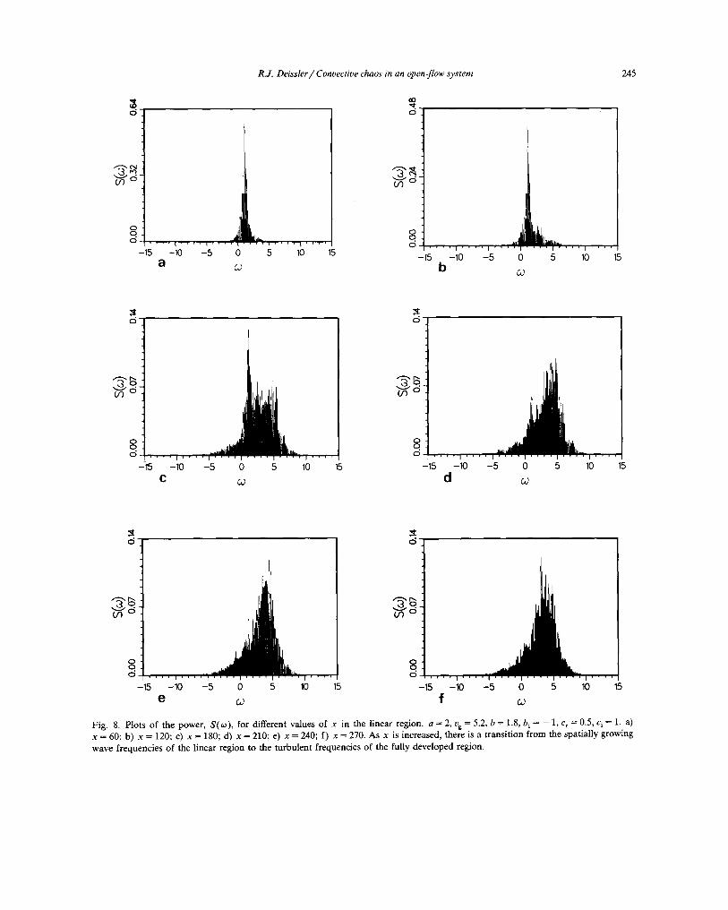
This transition from spatially growing wave frequencies to turbulent frequencies can be seen in fig. 8 which shows the power spectra at the same values of x as those in fig. 7. The spectra were calculated in the same way as those in the linear region. At x = 60 the signal is still dominated by the spatially growing wave frequencies, as can be seen by comparing fig. 8a with fig. 4d. As x is increased the spectra gradually shift to the turbulent frequencies until at x = 270 the peak corresponding to the spatially growing wave fre- quencie s can no longer be seen and the signal is dominated by the nonlinear dynamics, corresponding to a "fully developed turbulence".

As the system evolves, the extent of the coherent structure (i.e. sinusoidal structure) seen in fig. 2 changes with time, at times there being only a few regular waves and at other times there being many. Whenever the structure is coherent at a given spatial point, the time series at that point will be at the spatially growing wave frequencies since these are the frequencies at which the structure is driven. When the structure is irregular at a

244

I ,Q

300 I

320 a

R.J. Deissler

I I I

340 360 380

t

/Convective chaos in an open-flow system

400 300 320 340 360 380 400 b t

e O ~ '3

_~o -2o

300 320 340 360 380 400 300 320 340 560 380 400 c t d t

--2o

~ ) T ' I ' I ' I ' I ' I

`2o

? 300 320 340 360 380 400 300 320 340 360 380 400

e t f t

Fig. 7. Plots of ~r as a function of t for different values of x in the transition region and the fully developed region. a = 2 , vg=5.2, b r = l . 8 , b i = - l , c r=0.5 ,c i = l . a ) x = 6 0 ; b ) x=120;c ) x=180 ;d ) x=210 ;e ) x = 2 4 0 ; f ) x=270. Highandlow frequencies are seen to be interspersed. The fraction of the time that the signal is high frequency increases for larger values of x. The high frequency signals beginning at about t = 325, t = 350, and t = 385 (as seen in fig. 7b) are initiated by the more serious irregularities in the spatially growing waves (as seen in fig. 3d) beginning at about t = 310, t = 335, and t = 370.

g iven s p a t i a l po in t , the t ime series a t t ha t p o i n t

wi l l cons i s t o f the h igh f requenc ies g e n e r a t e d b y

the n o n l i n e a r d y n a m i c s . Thus the ne t effect wil l be

the i n t e r s p e r s i o n of h igh a n d low f requenc ies

in the t i m e ser ies as seen in fig. 7.

I f we a s s u m e a p l a n e - w a v e s o l u t i o n

~/( x , t ) = A e (ikx-i~°t) (19)

to eq. (1) w h e r e k a n d ~o are real , we f ind t ha t ~0,

k , a n d IA I a re r e l a t ed b y ~ o = i a + k v - i k 2 b -

i c l A [ 2. So lv ing for k a n d [A I gives ( f r o m ref. 8)

k =

[ ,l rc', )( t1 og ± o~ -- b i a i

2( brc---~i-Cr b i )

(20) a n d

IAI + ( .2-,1/2 = a ~ - K br) . (21)

P u t t i n g the p a r a m e t e r va lues f r o m the f igures in to


o o d _.~1

. . . . i , , , , I . . . . , -15 -10 - 5 0

a co

, , , ~ . . . . i . . . . 5 10 15

0o

o

o q o

-15 --10

b -5 0 5

GJ

10 15

X d

CO °

~t d

( / ) o

q o

--15 -10 - 5 0 5 10 15 -10 - 5 0 5

C ~ d

q o

-15 10 15

d d

o o o d d -

-15 -10 - 5 0 5 10 15 -15 -10 - 5 0 5 10 15

e ~ f

Fig. 8. P lo ts o f the power , S( t0) , fo r d i f ferent values o f x in the l inea r region , a = 2, vg = 5.2, b = 1.8, b i = - 1, c~ = 0.5, c i = 1. a) x = 60; b) x = 120; c) x = 180; d) x = 210; e) x = 240; f ) x = 270. A s x is inc reased , there is a t r an s i t i on f r o m the spa t ia l ly g r o w i n g

w a v e f r equenc i e s o f the l inear region to the t u r b u l e n t f requenc ies o f the ful ly deve loped region.


these equations, where the negative sign in eq. (20) is used and where ~0 is given by eq. (15), gives k = -0.408 and I A I = 1.844. These values agree well with the wavenumber and amplitude of the coherent portion of the structure seen in fig. 2. An important point here is that the wavenumber and amplitude of the coherent pattern formed depend on the frequency of the spatially growing waves, since this is the frequency at which the pattern is driven.

We can inquire into the stability of the coherent portion of the structure seen in fig. 2 just as we inquired into the stability of the equilibrium state q~ = 0. The coherent portion of the structure is clearly not absolutely unstable since, if it were, the irregular portion of the structure would work its way back until the whole structure were irregular. Also it dearly isn't absolutely stable since, if it were, the entire structure would be coherent. Therefore we conclude that the coherent portion of the structure is convectively unstable (i.e. a secondary convective instability).

Ref. 21 gives conditions to determine whether or not eq. (19) with periodic boundary conditions is a stable solution of eq. (1) (actually they treat the case of Vg = 0 but since the boundary conditions are periodic the stability criteria will be independent of %). As noted previously, the coherent portion of the structure in fig. 2 is convectively unstable. If periodic boundary conditions were instead imposed the structures would be absolutely unstable. Therefore if the stability conditions in ref. 21 were applied we would expect that they would give the result that the structures are unstable. For the parameter values of this paper we have 1 + bici/brc r < 0 (see eqs. (5.2) and (5.7) of ref. 21) which means that a sinusoidal structure of any wavenumber is unstable. This agrees with the previous observation that the coherent portion of the structure of fig. 2 is convectively unstable.

If the structure were driven by a single frequency corresponding to the pure spatially growing wave

~b(x, t) = Ce(# ~-i°''), (22)

where ~ is real and fir > 0, the entire structure would be coherent [satisfying eq. (19)] with a wavenumber and amplitude given by eqs. (20) and (21)[8]. However, since the coherent portion of the structure is convectively unstable, any deviation in the driving frequency from that of a pure spatially growing wave will cause the structure to break up at some spatial point. Referring to figs. 3d and 4d, we see that the structure of fig. 2 is not driven by a single frequency but is driven by a band of frequencies, the band being narrow enough to allow for the coherent portion of the structure seen in fig. 2. This band of frequencies corresponds to irregularities in the spatially growing waves (i.e. deviations from a pure spatially growing wave), which in turn correspond to variations in the amplitude, frequency, and /o r phase in the time series at a given spatial point (as can be seen in fig. 3d). These irregularities will travel down the structure (after being somewhat modified by the nonlinearity) and be spatially amplified (since the structure is convectively unstable) causing the structure to break up at some spatial point as seen in fig. 2. Now the point at which the structure breaks up will depend on the degree to which the spatially growing waves deviate from a pure spatially growing wave. As seen in fig. 3d, the degree of deviation from a pure spatially growing wave changes with time, causing the spatial point at which the structure breaks up to change with time. The result is intermittency.

For example, stretches of fairly constant frequency and amplitude can be seen in fig. 3d [which result in the formation of a fairly long coherent portion of the structure] interrupted by more serious changes in the frequency and amplitude [which will break up the coherent structure (at some spatial point) which was previously formed by the fairly regular stretch]. Comparing fig. 7b with fig. 3d, the more serious irregularities beginning at about t = 310, t = 335, and t = 370 in fig. 3d, for example, initiate the high-frequency signals beginning at about t = 325, t = 350, and t = 385, respectively, in fig. 7b.


(.9

(_9

O

-20 0 a

i

20 40 60

T

O ~5

-2( 0 20 40 60 80 b "r

o IC) o , - -06

(..9

O

-20 0 20 40 60 80 c "T

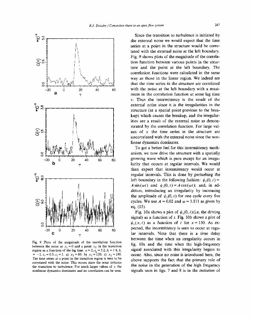
Fig. 9. Plots of the magnitude of the correlation function between the noise at x] = 0 and a point x 2 in the transition region as a function of the lag time. a = 2, vg = 5.2, br = 1.8, b i = - l , c r = 0 . 5 , c i = l . a) x 2=60; b) x 2=120; c) x 2=180. The time series at a point in the transition region is seen to be correlated with the noise. This occurs since the noise initiates the transition to turbulence. For much larger values of x the nonlinear dynamics dominates and no correlation can be seen.

Since the transition to turbulence is initiated by the external noise we would expect that the time series at a point in the structure would be correlated with the external noise at the left boundary. Fig. 9 shows plots of the magnitude of the correlation function between various points in the structure and the point at the left boundary. The correlation functions were calculated in the same way as those in the linear region. We indeed see that the time series in the structure are correlated with the noise at the left boundary with a maximum in the correlation function at some lag time ~-. Thus the intermittency is the result of the external noise since it is the irregularities in the structure (at a spatial point previous to the breakup) which causes the breakup, and the irregularities are a result of the external noise as demon- strated by the correlation function. For large values of x the time series in the structure are uncorrelated with the external noise since the nonlinear dynamics dominates.

To get a better feel for this intermittency mechanism, we now drive the structure with a spatially growing wave which is pure except for an irregularity that occurs at regular intervals. We would then expect that intermittency would occur at regular intervals. This is done by perturbing the left boundary in the following fashion: ~br(0, t) = Asin(c0t) and ~i(O,t)=Acos(~ot); and; in addition, introducing an irregularity by increasing the amplitude of ~r(0, t) for one cycle every five cycles. We use A = 0.02 and ~0 = 1.111 as given by eq. (15).

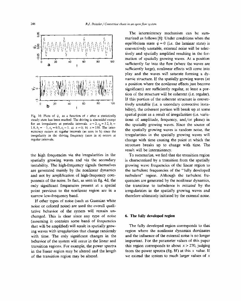
Fig. 10a shows a plot of ~br(0, t)(i.e, the driving signal) as a function of t. Fig. 10b shows a plot of ~Pr(X, t) as a function of t for x = 150. As expected, the intermittency is seen to occur at regular intervals. Note that there is a time delay between the time when an irregularity occurs in fig. 10a and the time when the high-frequency signal associated with this irregularity begins to occur. Also, since no noise is introduced here, the above supports the fact that the primary role of the noise in the generation of the high frequency signals seen in figs. 7 and 8 is in the initiation of

248 R.J. Deissler /Convective chaos in an open-flow system

o

5' 0 20 40 60 80 100

a f

~ - I ' i ' i ' i ' i ' / 0 20 40 60 80 100

b +

Fig . 10. P lo t s o f ~ r as a f u n c t i o n o f t a f t e r a s ta t i s t i ca l ly

s t e a d y s t a t e h a s b e e n r e a c h e d . T h e d r i v i n g is s i nuso ida l e x c e p t

fo r a n i r r e g u l a r i t y a t p e r i o d i c in te rva l s , a = 2, vg = 5.2, bf =

1.8, b i = - 1, c r = 0.5, c i = 1. a) x = 0; b ) x = 150. T h e in te r -

m i t t e n c y o c c u r s a t r e g u l a r i n t e rva l s (as seen in b) s ince the

i r r e g u l a r i t y in t he d r i v i n g f r e q u e n c y ( seen in a) o c c u r s at

r e g u l a r i n t e r v a l s .

the high frequencies via the irregularities in the spatially growing waves and via the secondary instability. The high-frequency signals themselves are generated mainly by the nonlinear dynamics and not by amplification of high-frequency components of the noise. In fact, as seen in fig. 4d, the only significant frequencies present at a spatial point previous to the nonlinear region are in a narrow low-frequency band.

If other types of noise (such as Gaussian white noise or colored noise) are used the overall qualitative behavior of the system will remain un- changed. This is clear since any type of noise (assuming it contains some band of frequencies that will be amplified) will result in spatially growing waves with irregularities that change randomly with time. The only significant changes in the behavior of the system will occur in the linear and transition regions. For example, the power spectra in the linear region may be altered and the length of the transition region may be altered.

The intermittency mechanism can be sum- marized as follows [8]: Under conditions when the equilibrium state q~ = 0 (i.e. the laminar state) is convectively unstable, external noise will be selectively and spatially amplified resulting in the formation of spatially growing waves. At a position sufficiently far into the flow (where the waves are sufficiently large), nonlinear effects will come into play and the waves will saturate forming a dynamic structure. If the spatially growing waves (at a position where the nonlinear effects just become significant) are sufficiently regular, at least a portion of the structure will be coherent (i.e. regular). If this portion of the coherent structure is convectively unstable (i.e. a secondary convective instability), the coherent portion will break up at some spatial point as a result of irregularities (i.e. variations of amplitude, frequency, and/or phase) in the spatially growing waves. Since the source of the spatially growing waves is random noise, the irregularities in the spatially growing waves will change with time causing the point at which the structure breaks up to change with time. The result will be intermittency.

To summarize, we find that the transition region is characterized by a transition from the spatially growing wave frequencies of the linear region to the turbulent frequencies of the "fully developed turbulent" region. Although the turbulent frequencies are generated by the nonlinear dynamics, the transition to turbulence is initiated by the irregularities in the spatially growing waves and therefore ultimately initiated by the external noise.

6. The fully developed region

The fully developed region corresponds to that region where the nonlinear dynamics dominates and the influence of the external noise is no longer important. For the parameter values of this paper this region corresponds to about x > 270, judging from the power spectra (fig. 8f) at this x value. If we extend the system to much larger values of x


we would expect little change in the behavior of the time series as x is increased.

The time series in fig. 7f indicates the existence of chaotic behavior in the fully developed region. Considering that in the deterministic limit (i.e. no external noise) the system is at rest (i.e. , = 0), does the notion of deterministic chaos even apply to such a system? As long as we restrict ourselves to the fully developed region, the answer to this question appears to be yes. For even though the structure is sustained by the presence of external noise, once this noise-sustained state is established we can restrict ourselves to the fully developed region where the overall macroscopic behavior is determined by the nonlinear dynamics.

Since perturbations can grow or decay depending on the frame of reference, one may expect problems in applying the usual measure of c h a o s - Liapunov exponents. In fact, as was dem- onstrated in ref. 15, if we were to naively apply the usual definition of Liapunov exponents to the system of fig. 2 we would find negative values for all the exponents even though a portion of the flow appears to be chaotic*. This occurs for the following reason: Even though two nearby trajectories may exponentially converge on the average in the stationary (i.e. laboratory) frame of reference, a moving frame of reference may exist in which nearby trajectories exponentially diverge on the average.

To make these ideas more concrete, we reiterate the definition of chaos for an open-flow system given in ref. 15. Let 8~k(x, t) be an infinitesimal perturbation about the state ~k(x, t). This perturbation satisfies the following equation:

v o~ff b ~2~ 38~ = aS~ - + - 2cl~lz/t~ Ot g-b-T Ox2

_ ( 2 3 )

*The reason that the exponents are negative is not due to a portion of the structure being regular, since if nearby trajectories are separating in any portion of a flow (in the stationary frame), the largest exponent for the whole system will be positive.

Consider an initial perturbation 8~k(x,0) localized in the region {x 1, x2}. We may define a velocity-

dependent Liapunov exponent (the largest one) as follows:

t - .~ f ( v , x 1,x 2,0) ' (24)

where

~'(v, xl , x 2 , t ) = x2+vt 12dx .

Here v refers to the velocity of the frame of reference from which the system is observed. For v > 0 the definition assumes that the system is unbounded in the + x direction. For v = 0 and for x 1 and x 2 corresponding to the boundaries of the system this definition reduces to the usual definition for the largest Liapunov exponent. Let v m be that v which gives the maximum value of

~(V; X1, X2). If ~(Vm; X1, X2) > 0, we say that the system is chaotic in the region { x 1 + vmt, x 2 + vmt }

and that k(Vn~; x 1, x2) is a measure of that chaos. The term chaos is appropriate in this definition

since the separation of trajectories - in some frame of r e fe rence- i s generated by the deterministic dynamics. Also, this definition should only be applied to the fully developed region of a flow. Finally, Ix2 - Xl[ is usually taken sufficiently large so that k is independent of x 2 and x r

As previously noted the usual definition of the Liapunov exponent gives a negative value. For the parameter values here we get k(0; 0, 300) = - 0.89 _+ 0.01 for the usual Liapunov exponent. This value was calculated by solving eq. (23) along with eq. (1). The noise is only added to eq. (1) and not to eq. (23) since the noise added to eq. (1) is independent of ~k and therefore does not contrib- ute a term to eq. (23) when ~b is varied. The reason that this value is negative is that, even though the perturbation 8~k may be initially growing, the perturbation is moving at a sufficiently large velocity so that both edges of the perturbation are moving in the same direction, allowing 8~k


behind the perturbation to approach zero (i.e. l i m t _ ~ 8 ~ ( x , t ) ~ 0 for an arbitrary fixed value of x in the interval (Xl, x2}). Thus the bulk of the perturbation eventually moves out through the right boundary leaving only its trailing edge which decreases with time.

Now allow the system of fig. 2 to extend to infinity in the + x direction. We can then let the region {x 1 + vt, x 2 + vt} move at different velocities v > 0. Remember that the perturbation 6qJ is initially localized within this region. If o is too small, the perturbation will "outrun" the region and X will be negative. If v is too large, the region will "out run" the perturbation and ?~ will again be negative. Therefore, ~ will have a maximum for some intermediate value of v. If this maximum value is positive, the fully developed region is defined as being chaotic with ~ as a measure of this chaos. Here we'll refer to this type of chaos (which is associated with perturbations growing only in a moving frame of reference) as convective

chaos to distinguish it from the usual type of chaos.

As pointed out in ref. 15, it is impractical to directly apply this definition to eq. (1) since the system would have to extend very far in the + x direction in order to get an accurate value for )~(v). In that reference, this problem was cir- cumvented by transforming the equation of motion [i.e. eq. (1)] into a frame of reference moving at velocity % and approximating open boundary conditions at both ends in order to simulate "moving with the fluid". This then gave a positive value of k. More generally, however, there may not be an obvious frame of reference in which to transform. We may generalize the idea of impos- ing periodic boundary conditions on a system in order to determine whether the system is convectively unstable (see last paragraph in section 2) as follows: If the largest Liapunov exponent ()~g) is negative for a given set of boundary conditions and the largest Liapunov exponent (hp) is positive for periodic boundary conditions imposed instead, then the fully developed portion of the flow is convectively chaotic and )~p is a measure of that

I• T ' I I ' I ' I ' I

0 50 100 150 200 250 300

X

Fig . 11. P lo t o f ~/r as a f u n c t i o n o f x fo r p e r i o d i c b o u n d a r y

c o n d i t i o n s a f t e r a s ta t i s t i ca l ly s t e a d y s t a t e ha s b e e n r e a c h e d .

a = 2, vg = 5.2, b r = 1.8, b i ~ - 1, c r = 0.5, c i = 1. T h i s s i m u l a t e s

a r e g i o n fa r d o w n s t r e a m .

chaos*. We assume that the dimensions of the system are sufficiently large so that part of the flow is fully developed.

As noted previously, for the parameter values of this paper h g = -0 .89 + 0.01. Putting periodic boundary conditions on the system, we find k p = 0.38 + 0.01. Since )~g < 0 and hp > 0, we conclude that the fully developed portion of the flow is convectively chaotic and that hp = 0.38 + 0.01 is a measure of that chaos.

In putting periodic boundary conditions on the system, we are simulating a region in the fully developed portion of the flow. Calculating the power spectra with periodic boundary conditions will then indicate the power spectra for the open flow at a point far down stream. Fig. 11 shows a plot of ~b as a function of x at a particular time t. Figs. 12 and 13 show plots of the time series and the power spectrum, respectively, at a point in the flow with periodic boundary conditions. Compar- ing fig. 13 with fig. 8f we see that there is some difference in the spectra indicating that the power spectra may change somewhat if we extend the system of fig. 2 to larger x values and examine a point further downstream. Nevertheless we will still characterize the flow at x = 270 as being fully developed since the bulk of the frequencies in figs. 8f and 13 lie in the same region and the peak

*If there is more than one basin of attraction, care must be taken to ensure that the flow with periodic boundary conditions is in the basin that correctly describes the fully developed portion of the flow with the given set of boundary conditions.

R.J. Deissler / Convectioe chaos in an open-flow system 2 5 1

0 20 40 60 80 100

f

r~

~1 1 ' i ' 1 , [ ' i ' ] 0 20 4 0 60 8 0 100

f

F i g . 12. P l o t o f ~k~ as a f u n c t i o n o f t a t x = 150 f o r p e r i o d i c

b o u n d a r y c o n d i t i o n s , a = 2, vg = 5.2, b r = 1.8, b i ~ - 1, c r =

0.5, c i = 1. T h i s s i m u l a t e s a t i m e se r i es f a r d o w n s t r e a m .

Fig. 14. Plot of ~kr as a function of t at x = 150 for periodic boundary conditions (with v = 0). a = 2, vg = 0, br = 1.8, b i

-1 , c~ =0.5, c i = 1. This simulates a time series far downstream in a co-moving frame of reference.

d

°L o. o

- 1 5 - 1 0 - 5 0 5 10 15

CA

Fig. 13. Plot of the power as a function of frequency corresponding to the time series seen in fig. 12. a = 2, vg = 5.2, b r 1.8, b~ = - 1, c~ = 0.5, c i = 1.

O

d

o d

-15 -10 -5 0 5 10 15 CA

Fig. 15. Plot of the power as a function of frequency corresponding to the time series seen in fig. 14. a = 2, vg = O, b r = 1.8, b i = - 1, C r = 0 . 5 , C i = L

c o r r e s p o n d i n g to the spat ia l ly growing wave fre-

quencies is no t seen in fig. 8f. Since no external

noise was a d d e d in the run with per iod ic b o u n d a r y

cond i t ions , the above suppor ts the fact that the

high f requencies seen in figs. 7 and 8 are genera ted

m a i n l y by the nonl inear dynamics and not by

ampl i f i ca t ion of high-frequency componen t s of the

noise.

I t m a y also be of interest to calculate the spec-

t ra for the flow in a moving f rame of reference.

This is done b y t ransforming eq. (1) to a f rame of

re ference mov ing at veloci ty vg, which is equivalent

to solving eq. (1) wi thout the convect ive term. We

aga in impose per iod ic b o u n d a r y condi t ions . Figs.

14 and 15 show a t ime series and the resul t ing

p o w e r spec t rum, respectively. Compar ing these

wi th figs. 12 and 13, we see that the t ime series in

the mov ing f l ame is more regular than that in the

s t a t i ona ry f l a m e of reference and also that the

s p e c t r u m is m o r e narrow. The reason that the t ime

series in the s ta t ionary f rame is more i r regular is

due to the spa t ia l s t ructure (fig. 11) being very

i r regular . There fore as this i r regular s t ructure

moves by with velocity vg (as observed in the

s t a t i ona ry f r ame of reference), the t ime series at a

s t a t i ona ry p o i n t will be very irregular.

I t is in teres t ing to ask quest ions (s imilar to

those above) abou t the flow when the left b o u n d a r y

is p e r t u r b e d per iodica l ly as in fig. 10a. In this case,

even though the t ime series at a po in t far down-

s t r eam (in the s ta t ionary f rame of reference) will

be high f requency, the signal will have a bas ic

p e r i o d equal to the basic per iod of the dr iving

252 RJ. Deissler / Convective chaos in an open-flow system

signal (fig. 10a). However, in a moving frame of reference the time series will be chaotic since nearby trajectories are diverging*. Therefore, we have the interesting case of a time series which is periodic in the stationary frame of reference, yet chaotic in a moving frame of reference. This assumes that there is no external noise in the system. If there is in addition some external noise in the system, noise will be amplified as it moves downstream (since nearby trajectories are diverging in a moving frame) and the time series will then be aperiodic in the stationary frame at a point sufficiently far downstream. In other words, in order to have an aperiodic signal at some point (sufficiently far downstream) in the stationary frame of reference, there must be at least some aperiodic component in the external driving.

To summarize, the fully developed region is characterized by high frequency turbulence which is generated by the deterministic equations of motion. The separation of nearby trajectories- in- dicating chaos - may only occur in a moving frame of reference.

7. Fluid systems

The behavior seen in this system is very similar to that seen in some open-flow fluid systems. For example, fluid flow over a flat plate also exhibits three distinct spatial regions: 1) a linear region in which Tollmien-Schlichting waves form as a result of a spatial and selective amplification of random background fluctuations [22-25]; 2) a transition region in which intermittent turbulence occurs [23, 24]; and 3) a fully developed turbulent region.

In the transition region high and low frequencies are seen to be interspersed, with the high frequencies occurring for a greater fraction of the time at a point further downstream from the leading edge of the plate. This sort of behavior is identical with the behavior occurring in the system

*This assumes (and it has been observed) that the structure is aperiodic in space at a given time.

studied in this paper. The question then arises as to the importance of the small fluctuations (near the leading edge of the plate) in the intermittency observed. A very similar intermittency mechanism could be occurring here with the irregularities in the Tollmien-Schlichting waves causing the waves in the nonlinear region to break up at different spatial points depending on the degree of irregularity in the ToUmien-Schlichting waves. In fact, experiments by Schubauer and Klebanoff [23] indicate that turbulent bursts are associated with variations in amplitude of the Tollmien- Schlichting waves.

Also, although the question of external noise is not addressed and no distinction is made between absolute and convective instabilities, the studies done in refs. 26 and 27 on some fluid systems lend strong support to this intermittency mechanism. Quoting ref. 26, the instability process examined there involved essentially three steps: 1) "primary (linear) instability of the basic shear flow"; 2) "nonlinear saturation of the primary instability and formation of a secondary flow"; 3) "see- ondary instability, i.e. linear instability of the secondary flow". These three steps occur in the Ginzburg-Landau system studied in this paper.

In addition, the experimental studies of refs. 28 and 29 discuss the existence of secondary instabilities. In particular, quoting ref. 29 (which deals with plane Poiseuille flow), the results there have "conclusively verified the validity of the concept of secondary instability." Finally, ref. 28 found that the length of the transition region became much shorter if very regular Tollmien-Schlichting waves were introduced by means of a vibrating ribbon (compared to the transition region of the naturally occurring Tollmien-Schlichting waves). This supports the intermittency mechanism since the irregularities in the more regular waves would vary less causing the spatial point at which the waves break up to vary less resulting in a shorter transition region.

It may be worthwhile to restate the intermittency mechanism in slightly different terms. In a


system for which the laminar state is convectively unstable, random background fluctuations are spatially and Selectively amplified resulting in the formation of spatially growing waves. Since the source of the spatially growing waves is random noise, the spatially growing waves will have irregularities (i.e. variations in frequency, amplitude, and or phase) that change with time. When the amplitude of the spatially growing waves becomes sufficiently large, nonlinear effects enter and a secondary flow is formed which itself is convectively unstable. Due to the fact that it is convectively unstable, the secondary flow will break up at some spatial point causing higher-frequency components to be generated by the nonlinear dynamics. Since the spatially growing waves have irregularities that change with time, the point where the secondary flow breaks up will change with time resulting in intermittency.

Also, as suggested by ref. 26, in fluid systems there may also be tertiary instabilities and so on. This would mean that the convectively unstable structure of the last paragraph would bifurcate into a new convectively unstable structure and so on until the last convectively unstable structure bifurcates into a turbulent structure. The same basic intermittency mechanism can still apply with the irregularities in each succeeding structure causing the point where one structure bifurcates into the next to change with time.

A few points should be mentioned about fluid systems. First, the nature of many of the instabilities in fluid flow is inherently three dimensional, a property which the one-dimensional Ginzburg- Landau equation is incapable of modeling. Nev- ertheless, the above-mentioned intermittency mechanism can still apply with the spatial point at which turbulent bursts form varying also in a direction perpendicular to the flow (depending on irregularities in the spatially growing waves perpendicular to the flow). Second, even if there were no irregularities in the spatially growing waves (i.e. a pure spatially growing wave) for a fluid system, the secondary (or tertiary, etc.) flow which

forms would probably still break up*. In this case, the spatial points at which the bursts form would not change with time and the bursts would occur at a frequency related to the frequencies present in the flow at a spatial point previous to breakup (e.g. the spatially growing wave frequency). How- ever, for a fluid system with irregular spatially growing waves the intermittency mechanism of the previous paragraphs can again still apply if the irregularities in the spatially growing waves are sufficiently large. The positions at which the bursts form would then change with time. The possibility of the second point is supported by ref. 28 where it was found, as previously noted [three paragraphs ago], that the transition region is much shorter if very regular Tollmien-Schlichting waves are introduced by means of a vibrating ribbon (compared to the transition region of the naturally occurring Tollmien-Schlichting waves).

There are a number of ways to study whether the random background fluctuations are responsible for the intermittency observed in experimental fluid systems. One would be a numerical simulation of the fluid equations in the presence of external noise for a system such as plane Poiseuille flow, fluid flow over a flat plate, or channel flow. Such a simulation, however, may be very difficult with the existing computer systems. With experimental fluid systems it may be possible to measure the correlation function between a point in the transition region and a point in the linear region. Also one may be able to artificially introduce very regular spatially growing waves with controlled irregularities as was done in this paper.

As mentioned in the introduction, plane Poiseuille flow [5] and wind-induced water waves

*For example, this type of behavior occurs in the Ginzburg-Landau equation if a small term proportional to ~2 is added to eq. (1). In this case a plane wave is no longer an exact solution and the regular structure will break up into higher frequencies at some spatial point even if the structure is driven by a pure spatially growing wave. However, just as in the discussion near the end of section 6, the high frequency signal will have a basic period equal to the period of the driving signal.


[6] both can be reduced to eq. (1).* Putting the parameter values from those references into the stability condition (9) gives that these systems are convectively unstable by a large margin (at least near the critical Reynolds number). Therefore, if the incompressible Navier-Stokes equations are solved for these systems one would expect the formation of noise-sustained structures. To see how the Reynolds number appears in eq. (1) for a physical system, for wind-induced water waves the parameter values in eq. (1) are related to the corresponding parameters of ref. [6] as follows: a = [ R - R c ] d l ; %= - a l ; b=a2; and c= ] R - R¢}dlrx, where R~ is the critical Reynolds number and the parameter values are given in tables 7-10 of ref. 6.

Refs. 17, 18 and 30 develop formalism to determine whether plasma and fluid systems are convectively unstable. Therefore these references can be used to determine the likelihood of noise- sustained structures in certain plasma and fluid systems.

Since Reynolds 1883 experiment was concerned with fluid flow in a pipe with circular cross section, a few words about this type of flow may be in order. Circular pipe flow differs from plane Poiseuille flow and the Ginzburg-Landau system studied in this paper in that the laminar state can only be linearly convectively unstable in a region where the profile is not yet fully developed (i.e. the inlet region), assuming that the fully developed laminar flow is (as is generally believed) linearly absolutely stable for all Reynolds numbers [31]. Therefore for the fully developed flow there are two basins of attraction (for sufficiently high Reynolds number). One corresponds to the laminar state and the other corresponds to a turbulent state. If a disturbance in fully developed laminar circular pipe flow is below a certain level, it will damp and settle into the laminar basin. If the disturbance is above a certain level, it will grow

*For plane Poiseuille flow c r < 0 and therefore the solution of eq. (1) does not saturate. However, the stability condition (9) involves only the lineafized equation.

and settle into the turbulent basin. This type of behavior has been observed experimentally [32, 33]. The fact that there are two basins allows for the existence of alternating laminar and turbulent regions along the length of the pipe. The turbulent regions are called slugs and were first observed by Reynolds [1]. Even though the flow is convectively unstable only in the inlet region, ideas presented in this paper can still apply. First, spatially growing waves (with irregularities that change with time) can still form in the inlet region as a result of the selective spatial amplification of small fluctuations originating near the pipe entrance. Second, the spatial points at which turbulent spots form may depend on the irregularities in the spatially growing waves. However, instead of more spots forming and coalescing further downstream (as, for example, in flat-plate flow), the spots will grow into turbulent slugs [34] (i.e. settle into the turbulent basin), while the waves between the spots will damp and form the laminar regions (i.e. settle into the laminar basin).

The above behavior may be modeled in a generalization of the Ginzburg-Landau equation by changing the sign of the cubic term in eq. (1) to cause explosive growth and by adding a quintic term to cause saturation [44]. In one spatial region the coefficient of the linear term can be taken positive (producing an "inlet region") and in another region it can be taken negative (resulting in two basins of attraction and the existence of slugs).

Before closing this section it may be relevant to mention a point about experimental fluid systems. In experimental setups, the turbulence downstream can modify the fluctuations at a point upstream due to pressure waves (produced by the turbulence) which will travel upstream and possi- bly due to vibration of the apparatus caused by the turbulence. This adds a richness-and complexity- not present in the system considered in this paper. An interesting question is whether or not the pressure waves produced by turbulent spots and slugs can significantly modify the fluctuations further upstream and therefore have a


significant effect on the dynamics of spot and slug formation. For example, although this is highly speculative, an interplay between the turbulence downstream and the fluctuations upstream could, in some cases, play a role in the formation of turbulent slugs. In this scenario, the fluctuation level near the entrance to the pipe would be modulated by the turbulent slugs further downstream (via pressure waves). When the fluctuation level is above a certain level, the fluctuations would be amplified sufficiently in the inlet region for the system to settle into the turbulent basin further downstream and produce a slug. When the fluctuation level is below a certain level, the fluctuations would not be sufficiently amplified and the system would settle into the laminar basin and produce a laminar region.

8. Conclusions

The time-dependent generalized Ginzburg- Landau equation was studied under conditions when it was convectively unstable. Under these conditions it models an open-flow system. In the presence of low-level external noise, this system exhibited three distinct spatial regions: 1) A linear region which is characterized by the selective and spatial amplification of the external noise resulting in the formation of spatially growing waves. 2) A transition region which is characterized by the transition from spatially growing wave frequencies to turbulent frequencies. In particular this region exhibits intermittency in which the random nature of the external noise plays a crucial role. 4) A fully developed region which is characterized by high frequency turbulence which is generated by the nonlinear dynamics. This region may be convectively chaotic which means that the separation of nearby trajectories only occurs in a moving frame of reference.

A few other points are: 1) Since low-level (microscopic) external noise can play an important role in the macroscopic behavior of open-flow systems (e.g. the intermittency), it can be crucial

to include external noise in the modeling of these systems. In particular, open-flow fluid systems are many times studied in a co-moving frame of reference. Thus the effects that continuous external noise may have on the system are not included and much of the physics may be lost. 2) The behavior of the Ginzburg-Landau system is very similar to the behavior of some open-flow fluid systems. Therefore the study of this system can give insights into the workings of actual fluid systems and indicate directions for further research into turbulent fluid systems.

Acknowledgements

The author thanks R.G. Deissler, J. Farmer, K. Kaneko, W. Kerr, P. Lomdahl, and G. Mayer- Kress for helpful conversations. He also thanks R. Blackwelder, M. Goldstein, P. Huerre, and W. Saric for pointing out useful references and thanks R.G. Deissler, D. Farmer, P. Scott, and the referees for their reading of and helpful comments on the manuscript. This work was partially supported by the Air Force Office of Scientific Research under AFOSR grant #ISSA-84-00017.

Appendix A

The discrete Fourier transform

Consider a complex time series Z ( t ) for the time interval from t = 0 to t = T. Then we may write

z( t )= Wke -2"ik'/T (25) k = - o ¢

and the inverse

W k = L f T z ( t ) e 2~rikt/T T J o ~

(26)

The frequencies are given by ~k = 2 ~ r k / T and the power at frequency to k is given by S k = W~' W k.

256 R.J. Deissler / Convective chaos in an open-f low sys tem

If we sample the time every time step At then we can write t =jAt and T = NAt where j is the discrete time index and N is the number of points in the time series. The discrete-time version of eqs. (25) and (26) is then

N / 2 - 1

Zj= E (27) k = - N / 2

and its inverse

I N 1 Wk= ~ ~_. Zje 2'~ijk/N. (28)

j=O

Since W k is periodic with period N (i.e. W k = Wk + N) we may write the sum in eq. (27) over any interval of N consecutive values of k. Since the fast Fourier transform is written from k = 0 to N - 1, the negative frequencies will appear in the interval N/2 to N - 1. The value of W k for the negative frequencies can be found from the relation W k = Wk+ N" We note that the negative frequencies are important here since the signal is complex and therefore the power spectrum, in general, is not symmetric about ~0 = 0.

Now consider two complex discrete time series Z U and Z2j over intervals from j = 0 to N - 1. Define the discrete correlation function as follows:

1 N - 1 C,= -~ Z Z~Zz(j+,)" (29)

j = O

It then follows that

N / 2 - 1

--Y" WlkWZk e - - . , . . . . - 2=ikt/lv , (30) C/ k = - N / 2

where Wlk and W2k are given by eq. (28). Eq. (29) can be easily shown by plugging Wlk and Wzk (from eq. (28)) into eq. (30) and using the relation ~ N / 2 1 e 2 ~ r i k ( j - j ' ) / N = NSj/. Fast Fourier trans-

k ~ -- N / 2

forms can be used to calculate the correlation function between two time series by first calculating Wtk and W2k from eq. (28) and then using eq.

(30) to calculate Q. If Zaj and Z 2 j are the same time series then eq. (29) is the auto-correlation function.

Appendix B

A few generalizations

In this section we note the stability conditions for a few generalizations of eq. (1). First consider a nonlinear partial differential equation which after linearization about the state + = 0 gives

0+ 4 0--/- = j=Z"oaY Ox J ~ " (31)

Then the solution of this equation may be written

+ ( x , t ) = / ~ d k A ( k ) e i k X e ~(k)t, (32)

where

1 o~ A(k) = ~-~ f dx'+o(x')e -ikx'

-- OQ

and

J a ( k ) = Y'. a j ( i k ) j.

j ~ 0

Here ~k0(x) is an initial localized perturbation about the state ~b = 0. We assume that ar(k ) --* - ~ and k ~ o¢ and as k --* - ~ . The stability conditions may be found using the method of steepest descent. Since a clear derivation is given in ref. 8, here we just quote the results. The system is absolutely unstable if

Re [a(k~)] > 0; (33)


R e [oL(km) ] ~ 0; (34)



R e [ a ( k ~ ) ] < 0 and R e [ a ( k m ) ] > 0 . (35)

Here k~ is the saddle point in the complex k plane and k m is the value of k on the real axis that gives the maximum value of a~. Therefore k~ is determined from d a / d k = 0 (k complex) and k m is determined from d a r / d k = 0 (k real). If a derivative gives more than one value for k, that value which gives the maximum % is chosen. For eq. (2) [where a(k ) = a - ikv - k2b], conditions (33) to (35) reduce to conditions (7) to (9).

A generalization of eq. (1) to two dimensions is

a# h d 02# 0~- = Vs-~- + + - cl~bl2g,. (36) i)x 2 i)y 2

Neglecting the nonlinear term, the solution of the linearized equation is

one would expect behavior similar to that of eq. (1). However, as a result of the added dimension, there can also be intermittency in the y direction which would be qualitatively more similar to fluid systems.

Appendix C

Coupled maps

A coupled-map lattice is a spatially-extended system that is discrete in both time and space [16, 35-43]. Although these systems do not result from a reduction of the fluid equations, they nevertheless can exhibit behavior similar to fluid systems and are very easily solved on a computer. Here we present a few analytical results that the author derived since ref. 16.

Consider the coupled-map lattice

t~(x, y , t ) = e at

4~rt ( bd )t/z

× dx'f dy' 0(x', y') - - ~ --00

× e-(X-Vt-X ' )2 /4bt

X e - ( y -y ' ) z /4d ' , (37)

where ~P0(x, y) is an initial localized perturbation about the state + = 0. This is derived in the same manner as eq. (6), except that there is a double Fourier integral. Applying the stability conds. (3), (4), and (5) (with the y variable included) we find that the stability conditions are identical with those of one space dimension [i.e. eqs. (7)-(9)]. Note that the moving frame of reference is in the x direction since the convective term in eq. (36) only depends on the first derivative in x thus causing a flow in the x direction. Also notice that the full nonlinear eq. (36) has a plane wave solution of the form A e (ikxx+ik>'y-i~°t) and that the linearized eq. (36) has a spatially growing wave solution of the form Ce(Bx+ik. vy-i~°t). Therefore

~'Xk+lY(l) : F ( g(k I), ~'kY(I-1), X k ( l + l ) ) . ( 3 8 )

Here k is discrete time, I is discrete space, and the number of points on the lattice is M (i.e. 1 < I < M). Let X0 (1) be a fixed-point solution of eq. (38). Then we may inquire into the linear stability of this solution by letting X~ ~) = X<o t) + 8X~/). 8X~ o will then satisfy the following equation:

6 x ( t ) a6X~l) + bSg(kl-1) + . 1 i ( / + 1 ) (39) k + l = t'~'~k '

where a=3F/3Xtk t), b=~F/3Xtk I-1), and c = 3F/~Xtk 1÷1). These derivatives are evaluated at the fixed point X0 u).

Let 2tg be the eigenvalue with the largest magnitude (for the given boundary conditions) and let h p be the eigenvalue with the largest magnitude (for periodic boundary conditions imposed instead). Then using the criteria given in the last paragraph of section 2 and in ref. 8, the equilibrium state will be absolutely unstable if

I~g[ > 1; (40)



I)~pl < 1; (41)

¢]S~ l) = ~keiBt implies ~ = a + b e -iB. In general,

given an initial perturbation 8X0 ~t), the solution is then


IXgl < 1 and I)~pl > 1. (42)

Note that the magnitude of the eigenvalue is the relevant quantity here since we are dealing with maps (discrete time).

If the given boundary conditions of eq. (38) are fixed boundary conditions at both ends (which implies that 8X~ I) = 0 at l = 0 and l = M + 1) then the Jacobian matrix will be the tridiagonal matrix ( b, a, e } where a are the diagonal elements and b and c are the elements below and above the diagonal, respectively. The eigenvalues of this matrix are

8X} t) = f02~d]3A(j3)(a + b e-i/~) k e it~', (45)

where

1 ~ ~X0(/')e -iBt'. (46) = 1 '= --otz

Putting (46) into eq. (45), using the binomial ex- pans ion (a + b e-J0) ~ = E , = o [ k ! / ( n ! ( k - n )!)] a k - , b n e - its,, and performing the integration

over/3 gives

k~ E

) ~ g s = a + 2 b ~ c o s , s = 1 , 2 . . . . . M.

(43)

For periodic boundary conditions the only difference in the Jacobian matrix will be the addition of the element b to the upper fight-hand corner and the element c to the lower left-hand corner due to the boundaries being coupled together. The eigenvalues of this matrix are

)kps -~- a + b e - 2 ~ r i s / M + c e 2rtis/M,

s = 0 , 1 , . . . , M - 1. (44)

These eigenvalues are given in ref. 8. For given values of a, b, and c we can then use eqs. (40)-(44) to determine the stability conditions of the equilibrium solution of eq. (38).

For one-way coupling (i.e. c = 0) the results are particularly simple. We then find that the system is absolutely unstable if ]a[ > 1, absolutely stable if l al + I bl < 1, and convectively unstable if both lal < 1 and lal + Ibl > 1.

For c = 0 we can also find an analytic solution for eq. (39). Assuming a solution of the ,form

× a(k-t+l'~b~l-~'), (47)

where O < l - l ' < k . For l - l ' <O or l - l ' > k, 8X~t)=0. If the single point l ' = 0 is initially perturbed by one unit we get

k~ °"'°~'X') = t ! ( k - Z)!

ak-lbt , (48)

where 0 < l < k. For l < 0 or 1 > k, 8X~ l) = 0. Transforming into a frame of reference moving

at velocity v by letting 1 = [vk] where the brackets mean " the integer part of" and where 0 < v < 1 gives ~X~ l) = ( k ! / ( [ v k ] ! ( k - [vk])!)}ak-[Vklb f°kl.

For simplicity lets now assume a > 0 and b > 0. Taking the limit as k ~ ~ gives (after replacing n! by n" e - " and simplifying) X~ t) = y~ where y = ( b / v ) ° ( a / ( 1 - v)) I-v. In the stationary frame of reference (i.e. v = 0), "r = a. Therefore the perturbation will damp at a given stationary point if a < 1. The maximum value of y occurs when v = b / ( a + b). The velocity of the perturbation for large k is then v = b / ( a + b). Putting this value of v into "y gives y = a + b. If a + b > 1 the perturbation will grow in the moving frame. Therefore the

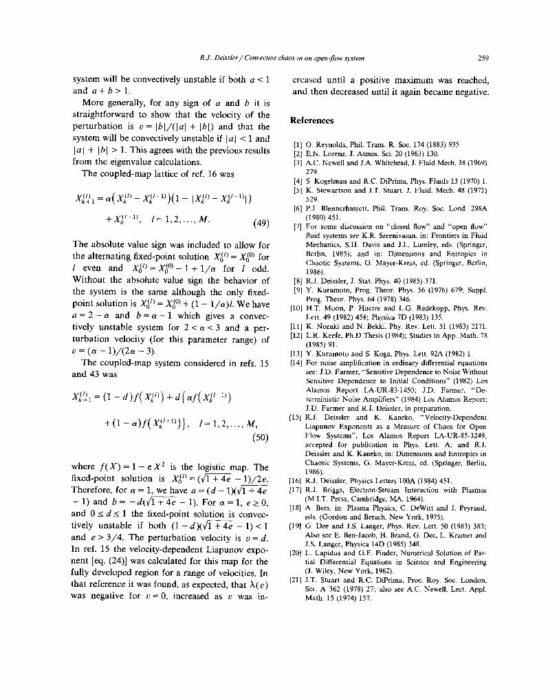
R.J. Deissler/ Convective chaos MI an open-jaw system 259

system will be convectively unstable if both a < 1 creased until a positive maximum was reached, and a+b> 1. and then decreased until it again became negative.

More generally, for any sign of Q and b it is straightforward to show that the velocity of the perturbation is u= Ibl/(lal + lbl) and that the system will be convectively unstable if [a( -C 1 and )(II + I bl > 1. This agrees with the previous results from the eigenvalue calculations.

The coupled-map lattice of ref. 16 was

References

PI PI [31

[41

[51

161

[71

0. Reynolds, Phil. Trans. R. Sot. 174 (1883) 935.

E.N. Lorenz, J. Atmos. Sci. 20 (1963) 130.

A.C. Newell and J.A. Whitehead, J. Fluid Mech. 38 (1969)

279.

S. Kogelman and R.C. DiPrima, Phys. Fluids 13 (1970) 1.

K. Stewartson and J.T. Stuart. J. Fluid. Mech. 48 (1971) xpl = a( xp_ x,(‘-l))(l - pq” _ J&w),)

+ &t- 1) ) f=1,2 )...) M. (49

The absolute value sign was included to allow for the alternating fixed-point solution X,$/J = X$‘) for I even and Xi’) = X,j’) - 1 + l/a for I odd. Without the absolute value sign the behavior of the system is the same although the only fixed- point solution is X4” = X,$‘) + (1 - l/a)/. We have a = 2 -(Y and b=a - 1 which gives a convectively unstable system for 2 < (Y < 3 and a perturbation velocity (for this parameter range) of u = (n - 1)/(2a - 3).

The coupled-map system considered in refs. 15 and 43 was

xj$ = (1 - d)f( x,(Q) + d{ fff( xp)

+ (1 - (Y)f( xk(‘+ “>L 1=1,2 )...) M,

(50)

where f(X)=l-eX* fixed-point solution is Therefore, for (Y = 1, we

is the logistic map. The x0”’ = (&z - 1)/2e. have a = (d - l)(\ll-t4e

- 1) and b = -d(p&% - 1). For (Y = 1, e 2 0, and 0 I d 5 1 the fixed-point solution is convectively unstable if both (1 - d)(dm - 1) < 1 and e > 3/4. The perturbation velocity is u = d. In ref. 15 the velocity-dependent Liapunov exponent [eq. (24)] was calculated for this map for the fully developed region for a range of velocities. In that reference it was found, as expected, that h(u) was negative for u = 0, increased as v was in-

PI

[91

IlOl

Pll

WI

1131

/I41

[I51

529.

P.J. Blennerhassett, Phil. Trans. Roy. Sot. Lond. 298A

(1980) 451.

For some discussion on “closed flow” and “open flow”

fluid systems see K.R. Sreenivasan, in: Frontiers in Fluid

Mechanics, S.H. Davis and J.L. Lumley, eds. (Springer,

Berlin, 1985); and in: Dimensions and Entropies in

Chaotic Systems, G. Mayer-Kress, ed. (Springer, Berlin,

1986).

R.J. Deissler, J. Stat. Phys. 40 (1985) 371.

Y. Kuramoto, Prog. Theor. Phys. 56 (1976) 679; Suppl.

Prog. Theor. Phys. 64 (1978) 346.

H.T. Moon, P. Huerre and L.G. Redekopp, Phys. Rev.

Lett. 49 (1982) 458; Physica 7D (1983) 135.

K. Nozaki and N. Bekki, Phy. Rev. Lett. 51 (1983) 2171.

L.R. Keefe, Ph.D Thesis (1984); Studies in App. Math. 78

(1985) 91.

Y. Kuramoto and S. Koga, Phys. Lett. 92A (1982) 1.

For noise amplification in ordinary differential equations

see: J.D. Farmer, “Sensitive Dependence to Noise Without

Sensitive Dependence to Initial Conditions” (1982) Los

Alamos Report LA-UR-83-1450; J.D. Farmer, “De- terministic Noise Amplifiers” (1984) Los Alamos Report; J.D. Farmer and R.J. Deissler, in preparation.

R.J. Deissler and K. Kaneko, “Velocity-Dependent

Liapunov Exponents as a Measure of Chaos for Open

Flow Systems”, Los Alamos Report LA-UR-85-3249,

accepted for publication in Phys. Lett. A; and R.J.

Deissler and K. Kaneko, in: Dimensions and Entropies in

Chaotic Systems, G. Mayer-Kress, ed. (Springer, Berlin, 1986).

[16] R.J. Deissler, Physics Letters 1OOA (1984) 451.

[17] R.J. Briggs, Electron-Stream Interaction with Plasmas

(M.I.T. Press, Cambridge, MA, 1964).

[18] A. Bers, in: Plasma Physics, C. Dewitt and J. Peyraud,

eds. (Gordon and Breach, New York, 1975).

[19] G. Dee and J.S. Langer, Phys. Rev. Lett. 50 (1983) 383;

Also see E. Ben-Jacob, H. Brand, G. Dee, L. Kramer and

J.S. Langer, Physica 14D (1985) 348. [20] L. Lapidus and G.F. Pinder, Numerical Solution of Par-

tial Differential Equations in Science and Engineering

(J. Wiley, New York, 1982).

1211 J.T. Stuart and R.C. DiPrima, Proc. Roy. Sot. London,

Ser. A 362 (1978) 27; also see A.C. Newell, Lect. Appl.

Math. 15 (1974) 157.


[22] H. Schlichting, Boundary-Layer Theory (McGraw-Hill, New York, 1968).

[23] H.L Dryden, in: Turbulent Flows and Heat Transfer, C.C. Lin, ed. (Princeton Univ. Press, Princeton, NJ, 1959).

[24] F.M. White, Viscous Fluid Flow (McGraw-Hill, New York, 1974).

[25] M.E. Goldstein, J. Fluid Mech. 154 (1985) 509. [26] S.A. Orszag and A.T. Patera, J. Fluid Mech. 128 (1983)

347. [27] S.A. Orszag, R.B. Pelz, and B.J. Bayly, "Secondary Insta-

bilities, Coherent Structures, and Turbulence", AIAA-85- 1486-CP, A1AA 7th Computational Fluid Dynamics Con- ference.

[28] ES. Klebanoff, K.D. Tidstrom and L.M. Sargent, J. Fluid Mech. 12 (1962) 1,

[29] M. Nishioka, M. Asai and S. Iida, in: Laminar-Turbulent Transition, R. Eppler and H. Fasel, eds. (Springer, Berlin, 1980).

[30] P. Huerre and P.A. Monkewitz, J. Fluid Mech. 159 (1985) 151.

[31] A.M.O. Smith, J. Fluid Mech. 7 (1960) 565; Also see J.T. Stuart, in: Laminar-Turbulent Transition, R. Eppler and H. Fasel, eds. (Springer, Berlin, 1980).

[32] Y. Rubin, I. Wygnanski and J.H. Haritonidis, in: Laminar-Turbulent Transition, R. Eppler and H, Fasel, eds. (Springer, Berlin, 1980).

[33] R. Teitgen, in: Laminar-Turbulent Transition, R. Eppler and H. Fasel, eds. (Springer, Berlin, 1980).

[341 1,J. Wygnanski and F.H. Champagne, J. Fluid Mech. 59 (1973) 281.

[35] J. Crutchfield, "Noisy Chaos", Ph.D. Thesis (1983). [361 K. Kaneko, Prog. Theor. Phys. 72 (1984) 480; see also

Ph.D Thesis (1983), to be published by World Sci. Pub. Co. (Singapore).

[37] K. Kaneko, Prog. Theor. Phys. 74 (1985) 1033. [38] J. Crutchfield and K. Kaneko, "Statistical Mechanics of

Lattice Dynamical Systems", in preparation. [39] R. Kapral, Phys, Rev. A 31 (1985) 3868. [40] Y. Aizawa, Prog. Theor. Phys. 72 (1984) 662. [41] T. Yamada mad H. Fujisaka, Prog. Theor. Phys. 73 (1985). [42] J. Keeler and D. Farmer, in preparation. [43] K. Kaneko, Phys. Lett. A 111 (1985) 321. [44] R.J. Deissler, "Turbulent Bursts, Spots, and Slugs in a

Generalized Ginzburg-Landau Equation", Los Alamos Report LA-UR-86-2067, submitted to Phys. Lett. A.

[45] T. Nita, I. Met. Soc. Japan 40 (1962) 13.

spatially growing waves, intermittency, and convective chaos in an open-flow system

Documents