Pages 191-203 in J.C. Grégoire, A.M. Liebhold, F.M. Stephen, K.R. Day, and S.M. Salom, editors. 1997.Proceedings: Integrating cultural tactics into the management of bark beetle and reforestation pests. USDAForest Service General Technical Report NE-236.

Spatio-temporal geostatistical analysis of Ips typographusmonitoring catches in two Romanian forest districts.

LAURENT RATY1, CONSTANTIN CIORNEI2 AND VASILE MIHALCIUC3.

1Laboratoire de Biologie animale et cellulaire, Université Libre de Bruxelles, Bruxelles, Belgium2Institute for Forest Research and Planning (ICAS), Station Bacau, Romania

3Institute for Forest Research and Planning (ICAS), Station Brasov, Romania

ABSTRACT Systematic trapping and monitoring of the spruce bark beetle Ips typographus has been carried outextensively in the Romanian Carpathians since 1984, using pheromone traps. We present here a geostatisticalanalysis of catches performed in two contiguous Romanian forest districts, Rastolita and Lunca Bradului.Numbers of insects caught per trap between 1987 and 1994 were aggregated over each year. These datapresented very good spatial, and good temporal auto-correlation. Because of their strongly left skeweddistribution, analyses were performed on logarithm of the catches. Data were spatially detrended by a median-polish., that produced spatially isotropic residuals. Isolated spatial outliers were Winsorized through robustkrigings based on omni-directional variograms, and performed separately over each year. A global spatio-temporal (anisotropic) variogram was then fitted to Winsorized data, and kriging estimates were built. It waspossible to estimate catch logarithm, using spatial kriging, with relative precision ranging around 10%, takinginto account results of only the current year. More interestingly, spatio-temporal kriging also performed well toforecast logarithmic catch, using results from three previous years. In spatio-temporal kriging, auto-correlationbetween measurements spaced too closely introduced a loss of information. A theoretical analysis of the spatio-temporal variogram showed that, when kriging neighbourhood is limited in terms of number of data used toforecast next-year catches (thus when computation effort is limited), an optimal trap density may be calculated.

KEY WORDS Ips typographus, Romania, geostatistics, interpolation, forecast, monitoring

THE SPRUCE BARK BEETLE, Ips typographus (Coleoptera: Scolytidae), is a semi-aggressivebark beetle that can kill extensive areas of spruce by the burrowing activities of its larvae,particularly after natural, weather-linked, phenomena such as drought and windthrow. Lossof vigour due to stressing agents such as these is a very common precursor to serious pestoutbreaks (Speight 1996). Control of this pest species is very difficult; sanitationmanagement of forests can reduce the impact of Ips typographus, though the sheer magnitudeof the outbreaks can render the operation unfeasible.

In the Romanian Carpathians (Moldavia and Transylvania), systematic trapping andmonitoring program of the spruce bark beetle has been carried out very extensively since1984. Pheromone-baited traps are now placed in virtually every forest likely to harbourinsect populations. The results produced by this program have provided a valuable source ofinformation concerning insect population fluctuations that might be related to climatic andbiotic conditions (weather, soil conditions, geography etc.). Hence, after appropriate andexhaustive analysis, these data provide an unparalleled opportunity to study the outbreakdynamics and effects of potential pest management strategies of one of the most importantinsect pests in Europe.

In this paper, we present a spatio-temporal geostatistical analysis of the catchesperformed in two contiguous Romanian forest districts, Rastolita and Lunca Bradului,

RATY ET AL.192

between 1987 and 1994. Our aims are to analyse the spatio-temporal variations of thesecatches (i.e. to see how catches vary spatially during each year, and how they vary from yearto year at a given place), and to build estimates of the catches for places and years where nomeasure is available.

It is well known that damage due to semi-aggressive bark beetles are dependant ontheir population density. In particular, colonisation of a tree will be successful only if thenumber of beetles able to aggregate on that tree is high enough to overcome its defencereactions (i.e., Lieutier 1990). Assuming that trap efficiency does not vary too much fromplace to place or year to year, it seems logical to think to the number of insects caught in atrap is an indicator of the number of beetles crossing the trap neighbourhood and able torespond to their aggregative pheromone, e.g. able to aggregate on a host tree.

Building predictions of the catches for locations where no traps were set up might beuseful to foresters, as it would give them a tool to know where they need to focus on andprepare for possible attacks and help them to locate colonised trees to destroy beetles.Forecasting the catches would be useful as well, as this might provide a tool to decide whenand where preventive control methods might be usefully set up.

Data

Insect trapping data were produced by monitoring 300 permanent traps in the twoRomanian forest districts of Rastolita and Lunca Bradului. This area covers a total of about90,000 ha. Traps were black PVC drainpipe tubes 8 cm in diameter with numerous smallholes and a Typolur (Cluj, Romania) pheromone dispenser hung inside the tube. Dispenserswere set up at the beginning of the flight period and not renewed before next year. Attractedbeetles land on the tube, enter one of the holes and fall into a collector (usually a glass jarhalf-filled with water). These traps have been visited roughly on a weekly basis, dependingon accessibility of the location where the trap was set up, by Romanian forest employees.

Catches were combined for time each year to suppress temporal discontinuityinherent to insect catches made at short intervals (each catch is one discrete event).Summarizing data on a yearly basis also avoids problems that arise when comparing catchesperformed at different periods of the year, due to a decrease of pheromone-trap efficiency asthe dispenser dries out (Raty et al. 1995).

Romanian forest are divided in planning units that are defined as homogenous inregard to slope, orientation, soil characteristics, type of station and type of forest. Thisresults in a fairly large variation in the unit area, ranging from approximately 0.5 to 80 ha.

Our data initially associated traps to the planning units where they were set up. Toconvert these data into geographical co-ordinates, a Geographical Information System (GIS),Arc/Info, was used to digitise 1:20 000-scaled maps of the forest districts. Planning-unitboundaries were encoded in vectorial format, location of the centroids of the polygonsdelimited by these boundaries were computed, and each trap was associated to its planning-unit centroid. These results were used to produce an ASCII file associating aggregatedyearly catches to trap location and the year considered.

RATY ET AL. 193

Data analyses

We mostly used classical geostatistical tools, from which we will assume anelementary knowledge. Interested readers may find more complete and precise descriptionof these tools in Isaaks and Srivastava (1989) and in Cressie (1993). We generally used thesame notations as Cressie (1993). We think to our data as a partial realisation of a randomprocess, noted {Z(s) : s ∈ D} where s, the data location, varies continuously over D, which isa subset of the d-dimensional space ℜd (d = 2 when only space is considered and 3 whentime is taken into account). Data are noted {Z(s1), ..., Z(sn)}. All analyses were performedon the basis of the ASCII file described above, using FORTRAN 77 routines that were, inmost cases, written especially for this purpose.

Exploratory analyses

Exploratory Data Analysis (EDA) was introduced in spatial statistical analyses byTukey (1977), and has since become a classical precursory stage to geostatistical studies(Cressie 1993, Rossi et al. 1992). Its main goals are visualising data set, analysing datadistribution, investigating their stationarity and spatial (or spatio-temporal) continuity, anddetecting possible outlying data. EDA mostly uses simple statistical methods, such ascomputing means, medians and histograms. According to Cressie (1993), EDA may beusefully completed by more spatial analysis techniques, including computation of directionalvariograms, computation of pocket plots and median polishing.

Data skewness - Our data exhibited a strongly left skewed distribution. Furthermore, whencalculated over each year, catch mean was linearly correlated to catch standard deviation(r = 0.77; p = 0.02). These effects were corrected, as prescribed by Tukey (1977), withapplication of a logarithmic transformation (Z’ = ln Z).

Variograms and global non-stationarity - Observed directional spatial variograms wereestimated for each year separately, following 4 directions (N-S, NE-SW, E-W and NW-SE),using the classical estimator (Matheron 1962) :

∑ −≡)(

2))()(()(

1)(ˆ2

h

ssh

hN

ji ZZN

γ

A global pattern emerged from these computations. Variograms were fairly wellshaped, exhibiting very small nugget-effects (close to 0), apparent sills ranging between 0.8to 2 and apparent ranges between 4,000 and 8,000 m. At first glance, the data seem spatiallycontinuous, and do not show evidence of strong measurement errors. However, zonalanisotropy was always clearly present. The E-W and SE-NW directions showed consistentlyhigher sills than the two other directions. Furthermore, in these two directions, semi-variogram sills were typically larger than data variance. Combination of these twoobservations may be thought as evidence of global non-stationarity, and would indicatepresence of a spatial trend in the data. Furthermore, this trend might have a permanentcomponent, as patterns are comparable from year to year.

An observed temporal variogram was also estimated, with the whole data set. Thisvariogram exhibited an apparent nugget effect of close to 0.4. This is much larger thanspatial variograms, and may be due to significant variation in population density from year toyear. After this abrupt vertical jump, the variogram increased slowly. At the scale of our

RATY ET AL.194

study, it remained always smaller than twice the data variance (variance was 0.747; largestcomputed semi-variogram value, for a 4-years lag, was 0.408). This could be explained if wehypothesise a permanent spatial mean structure: in a purely temporal variogram, suppressedonly data from the same spatial location are compared. Variation within these data, evenwhen separated by large temporal lags, would be smaller than global variation.

Data detrending - From the above discussion, we will introduce the following modeldeveloped by Cressie (1993): assuming our data are partial realisation of a process thatsatisfies the following decomposition :

Z(s) = µ(s) + R(s) where µ(s) is a deterministic mean structure, called large-scale variation or trend and R(s) is astationary process, called small-scale variation. This kind of decomposition applied to a dataset is called detrending. Median polish (Tukey 1977) is an EDA technique designed toidentify large-scale and small-scale variation for gridded data, by analysing them as a 2- (orhigher-) way table, and using the following additive model :

data = global effect + row effect + column effect + residual.Decomposition follows an algorithm that alternatively sweeps medians out of rows andcolumns, and accumulates them in «row», «column», and «global» registers. A table ofresiduals results as well as preservation of additive decomposition relation at each step. Ifdata are non-gridded, a low-resolution grid may be overlaid onto the data map. Each datapoint may be assigned to the nearest grid node (Cressie 1993), and median polish performedon this grid. A complete trend surface can be built by planar interpolation between the gridnodes.

A 2 km x 2 km grid was overlaid onto the data map. Each trap was assigned to theclosest grid node and a spatial median polish was performed on this grid. To account for theapparently permanent character of the trend, we applied the algorithm only once, taking intoaccount catches performed during the 8 years simultaneously. This produced a median-polish trend surface, showing obvious large-scale variation in both E-W and N-S directions.

Observed directional spatial variograms were estimated for each year, on the basis ofthe median-polish residuals. Most of the spatial anisotropy was captured by the medianpolish. Next steps of our analyses will be performed on the median-polish residuals,assuming they behave isotropically in space.

The temporal variogram remained clearly unchanged by the spatial median polish.However, as global variance of the median-polish residuals (0.437) was lower than varianceof the original set of catch logarithms (0.747). The variogram values of the largest temporallags were now much closer to twice the sample variance.

Local non-stationarity - The pocket plot technique (Cressie 1993) was used to detectpockets of local non-stationarity in median-polish residuals reassigned to the 2km2 grid nodesthat were used for the median polish. These analyses were performed separately for eachyear, and showed the presence of pockets of non-stationarity in each year.

Spatial geostatistical analysesAll analyses were performed on the basis of median-polish residuals, treated as a

spatially isotropic data set. However, since we detected the presence of local pockets of non-

RATY ET AL. 195

stationarity in the last step of the exploratory analyses, we treat our data as a realisation of aGaussian stationary process.

As with Hawkins and Cressie (1984), we will consider R(s) as a mixture of astationary Gaussian sub-process and some other sub-process with heavy-tailed distribution.This last sub-process will act only on measurement errors and micro-scale variations, for asmall proportion of the global process (non-Gaussian contamination).

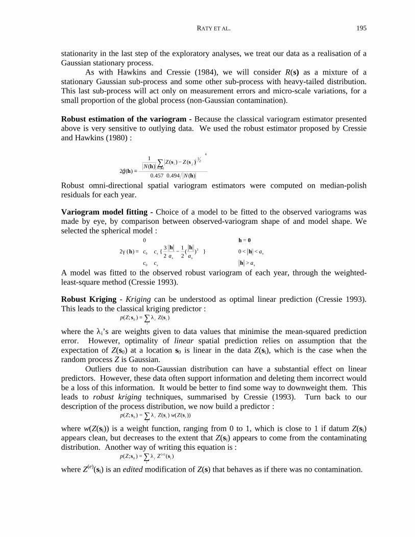
Robust estimation of the variogram - Because the classical variogram estimator presentedabove is very sensitive to outlying data. We used the robust estimator proposed by Cressieand Hawkins (1980) :

)(494.0457.0

)()()(

1

)(ˆ2

4

)(

21

h

ssh

hh

N

ZZN N

ji

+

−

≡∑

γ

Robust omni-directional spatial variogram estimators were computed on median-polishresiduals for each year.

Variogram model fitting - Choice of a model to be fitted to the observed variograms wasmade by eye, by comparison between observed-variogram shape of and model shape. Weselected the spherical model :

2

03

2

1

200

3

0

γ ( ) { ( ) }h

h 0h h

h

h

=

=

+ − < <

+ >

c ca a

a

c c a

ss s

s

s s

A model was fitted to the observed robust variogram of each year, through the weighted-least-square method (Cressie 1993).

Robust Kriging - Kriging can be understood as optimal linear prediction (Cressie 1993).This leads to the classical kriging predictor :

p Z Zi ii

( ; ) ( )s s0 = ∑λ

where the λi’s are weights given to data values that minimise the mean-squared predictionerror. However, optimality of linear spatial prediction relies on assumption that theexpectation of Z(s0) at a location s0 is linear in the data Z(si), which is the case when therandom process Z is Gaussian.

Outliers due to non-Gaussian distribution can have a substantial effect on linearpredictors. However, these data often support information and deleting them incorrect wouldbe a loss of this information. It would be better to find some way to downweight them. Thisleads to robust kriging techniques, summarised by Cressie (1993). Turn back to ourdescription of the process distribution, we now build a predictor :

p Z Z w Zi ii

i( ; ) ( ) ( ( ))s s s0 = ∑λ

where w(Z(si)) is a weight function, ranging from 0 to 1, which is close to 1 if datum Z(si)appears clean, but decreases to the extent that Z(si) appears to come from the contaminatingdistribution. Another way of writing this equation is :

p Z Zie

ii

( ; ) ( )( )s s0 = ∑λ

where Z(e)(si) is an edited modification of Z(s) that behaves as if there was no contamination.

RATY ET AL.196

The method we used is a geostatistical version of Huber’s procedure for robust time-seriesanalysis (1979, in Cressie 1993), but was performed with the robust variogram estimatorproposed by Hawkins and Cressie (1984). Models fitted to robust variogram estimators wereused to compute kriging weights for each R(sj) from all the remaining R(si). A prediction:

∑≠

− =ji

iijj ZR )()(ˆ ss λ

was built on basis of these weights and the associated error was computed. Using theseresults, the R(sj) were Winsorized. That is, they were replaced by an edited version such as:

R

R c

R

R c

R R c

R R c

R R c

ej

j j j j

j

j j j j

j j j j j

j j j j j

j j j j j

( ) ( )

$ ( ) ( )

( )$ ( ) ( )

( ) $ ( ) ( )

( ) $ ( ) ( )

( ) $ ( ) ( )

s

s s

s

s s

s s s

s s s

s s s

=+

−

− >

− ≤

− < −

− −

− −

− −

− −

− −

σ

σ

σ

σ

σ

if

if

if

Edited values were then used to compute a new robust observed variogram, to which a newmodel was fitted. This variogram served to perform a new Winsorization, and this procedurewas repeated until convergence of the edited values.

Depending on the year, 5 to 8% of the data were edited. Edited data may be separatedin two categories : real outliers (data with especially high or low values), and pairs of dataspatially very close together, but with differing values. Part of these last data were probablynot really outlying. Their outlying appearance may have been due to imprecision in thelocation associated to the data (the planning-unit centroids).

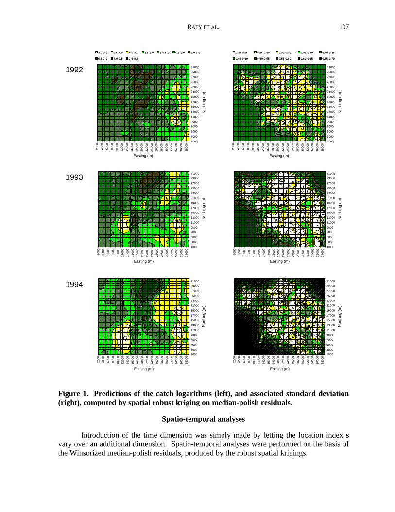
Winsorized data were used to build predictions and to estimate kriging error over thewhole study area, on a 500m2 grid. Summing these predictions to the median-polish trendsurface, we obtained prediction maps for the catch logarithms. It has been showed byCressie (1993), that error associated to these predictions is the kriging error associated to theresidual kriging predictions. Within the area where traps were set up, the prediction relativeprecision (estimated by the ratio of half 95%-confidence interval to the prediction) rarelyexceeded 10%. Maps of the predictions and the associated standard deviation for the years1992 to 1993 are presented in Figure 1.

RATY ET AL. 197

1992

1993

1994

2000

4000

6000

8000

1000

0

1200

0

1400

0

1600

0

1800

0

2000

0

2200

0

2400

0

2600

0

2800

0

3000

0

3200

0

3400

0

3600

0

3800

0

1000

3000

5000

7000

9000

11000

13000

15000

17000

19000

21000

23000

25000

27000

29000

31000

Easting (m)

Nor

thin

g (m

)

3.0-3.5 3.5-4.0 4.0-4.5 4.5-5.0 5.0-5.5 5.5-6.0 6.0-6.5

6.5-7.0 7.0-7.5 7.5-8.0

2000

4000

6000

8000

1000

0

1200

0

1400

0

1600

0

1800

0

2000

0

2200

0

2400

0

2600

0

2800

0

3000

0

3200

0

3400

0

3600

0

3800

0

1000

3000

5000

7000

9000

11000

13000

15000

17000

19000

21000

23000

25000

27000

29000

31000

Easting (m)

Nor

thin

g (m

)

2000

4000

6000

8000

1000

0

1200

0

1400

0

1600

0

1800

0

2000

0

2200

0

2400

0

2600

0

2800

0

3000

0

3200

0

3400

0

3600

0

3800

0

1000

3000

5000

7000

9000

11000

13000

15000

17000

19000

21000

23000

25000

27000

29000

31000

Easting (m)

Nor

thin

g (m

)

2000

4000

6000

8000

1000

0

1200

0

1400

0

1600

0

1800

0

2000

0

2200

0

2400

0

2600

0

2800

0

3000

0

3200

0

3400

0

3600

0

3800

0

1000

3000

5000

7000

9000

11000

13000

15000

17000

19000

21000

23000

25000

27000

29000

31000

Easting (m)

Nor

thin

g (m

)

2000

4000

6000

8000

1000

0

1200

0

1400

0

1600

0

1800

0

2000

0

2200

0

2400

0

2600

0

2800

0

3000

0

3200

0

3400

0

3600

0

3800

0

1000

3000

5000

7000

9000

11000

13000

15000

17000

19000

21000

23000

25000

27000

29000

31000

Easting (m)

Nor

thin

g (m

)

2000

4000

6000

8000

1000

0

1200

0

1400

0

1600

0

1800

0

2000

0

2200

0

2400

0

2600

0

2800

0

3000

0

3200

0

3400

0

3600

0

3800

0

1000

3000

5000

7000

9000

11000

13000

15000

17000

19000

21000

23000

25000

27000

29000

31000

Easting (m)

Nor

thin

g (m

)

0.20-0.25 0.25-0.30 0.30-0.35 0.35-0.40 0.40-0.45

0.45-0.50 0.50-0.55 0.55-0.60 0.60-0.65 0.65-0.70

Figure 1. Predictions of the catch logarithms (left), and associated standard deviation(right), computed by spatial robust kriging on median-polish residuals.

Spatio-temporal analyses

Introduction of the time dimension was simply made by letting the location index svary over an additional dimension. Spatio-temporal analyses were performed on the basis ofthe Winsorized median-polish residuals, produced by the robust spatial krigings.

RATY ET AL.198

Estimation of the spatio-temporal variogram - The robust variogram estimator developedby Cressie and Hawkins (1980) was used to compute an observed spatio-temporal variogram,for spatial lags from 0 to 10,000 m and temporal lags from 0 to 5 years (Figure 2a). In thespatial domain, variogram appeared very « clean », with nugget effect close to zero, andvalues growing slowly with the lag. An apparent sill was reached around 6,000 m, with avalue between 0.7 and 0.8, slightly lower than twice the sample variance (0.437). In thetemporal domain, nugget effect was clearly higher, and range was probably not reachedwithin the temporal scale of our study. Given that, in the space-time domain, the variogramreached values that are higher than the apparent spatial sill, temporal sill was probably higherthan this spatial sill.

Fitting of a spatio-temporal variogram model - Geometrical anisotropy is clearly inherentto any spatio-temporal variogram, as units are not the same along the space and time axes.Our data, however, showed clearly more complex behaviour than simple geometricalanisotropy : not only ranges differed between the axes, but also nugget effects and sillsdiffered. For anisotropy, the usual way is to search for a linear transformation of the co-ordinate system that would produce a reduced isotropic variogram (Isaaks and Srivastava1989, Cressie 1993).

To describe the spatio-temporal variogram of our data, we used a model with fouradditive structures : one pure nugget effect (2γ0), one structure accounting for the anisotropyin the nugget effects (2γ1(h1)), one accounting for geometrical anisotropy(2γ2(h2)), and thelast one accounting for zonal anisotropy (2γ3(h3)). These structures were all described byspherical variogram models :

2γ(h) = 2γ0 + 2γ1(h1) + 2γ2(h2) + 2γ3(h3),where :

2

03

2

1

20 1

1

3γ i i

i

i i i i

i i

w

w

( ) { ( ) }h

h 0

h h h

h

=

=

− < <

>

h T hii x

i ti

a i x

a i t

x

t

h

h

h

h=

= =

,

,

,

,

1

10

0

This model has 9 parameters, namely w0, w1, w2, w3, ax,1, at,1, ax,2, at,2, and at,3 (ax,3 is infinite,ax,0 and at,0 are zero).

However, to simplify fitting, we assumed some relations between them. γ1(h1)accounted for additional nugget effect observed in the time domain. Nugget effect may beviewed as result of measurement error plus result of variations at smaller scale than smallestlag : as measurement errors occurred both in the spatial and temporal domain, additionalnugget effect in the time domain had to be due to the other source. Within time domain,γ1(h1) needed therefore to have reached its range after one year, which was the shortesttemporal lag that we considered. To account for that, at,1 was set to 1 year. Both the purelyspatial and purely temporal variograms were well described by single spherical models (twoadditive models with different ranges did not improve significantly the fitting). Therefore,we set : ax,1 = ax,2 = ax and at,2 = at,3 = at. This left us with 6 parameters, that were estimatedthrough weighted-least-square fitting. A three-dimensional plot of the fitted model is shownin Figure 2b.

RATY ET AL. 199

0

600

1200

1800

2400

3000

3600

4200

4800

5400

6000

531

0

0,1

0,2

0,3

0,4

0,5

0,6

0,7

0,8

0,9

1

Spat ia l lag (m)

tempora l l ag

(years)

a. Observed variogram

0

600

1200

1800

2400

3000

3600

4200

4800

5400

6000

543210

0

0,1

0,2

0,3

0,4

0,5

0,6

0,7

0,8

0,9

1

Spat ia l lag (m)

tempora l l ag

(years)

b. Fitted variogram model

Figure 2. Spatio-temporal observed robust variogram computed on Winsorizedmedian-polish residuals (a), and model fitted to this variogram (b).

Spatio-temporal kriging - Two practical situations may justify the use of spatio-temporalkriging, rather than (much more simple) spatial kriging : (1) to build interpolation predictionsof the variable during one year where we have data, if it can improve the prevision precision,and (2) to forecast the variable for one year where no data are (yet) available. We will nowtake a look at these two situations.

Data values are not necessary to compute kriging weights and kriging error for thevariogram if we assume a design with given data location. Let us assume a trapping designwhere permanent traps are located on a regular square grid. Within this design, locationswhere kriging error is largest are the square centres. Therefore, we will pay attention to thesepoints. Kriging weights and error are functions of the location of the traps used to build theestimate that can let vary by changing the size of the grid squares. In this case, we vary thetrapping effort. Furthermore, they are functions of the kriging neighbourhood, that may beexpressed in terms of the number of traps used to build the estimate (spatial krigingneighbourhood), and of the number of years over which data are taken into account (temporalkriging neighbourhood). In this case, we vary the computation effort.

Taking only the symmetric spatial neighbourhoods into account, and restricting themto a reasonable number of data, a limited set of possibilities exists. The five smallestsymmetric spatial neighbourhoods of our case study are illustrated in Figure 6. Theyrespectively account of 4, 12, 16, 24 and 32 traps.

Spatio-temporal kriging used for interpolation - For the trapping device described above,kriging weights and error were computed, for distances between neighbouring traps varyingfrom 500 m to 5,000 m, by steps of 500 m, and taking account of data from the 5 smallestsymmetric spatial kriging neighbourhoods, first over the current year only, then over currentand one previous year and, lastly, over current and two previous years.

RATY ET AL.200

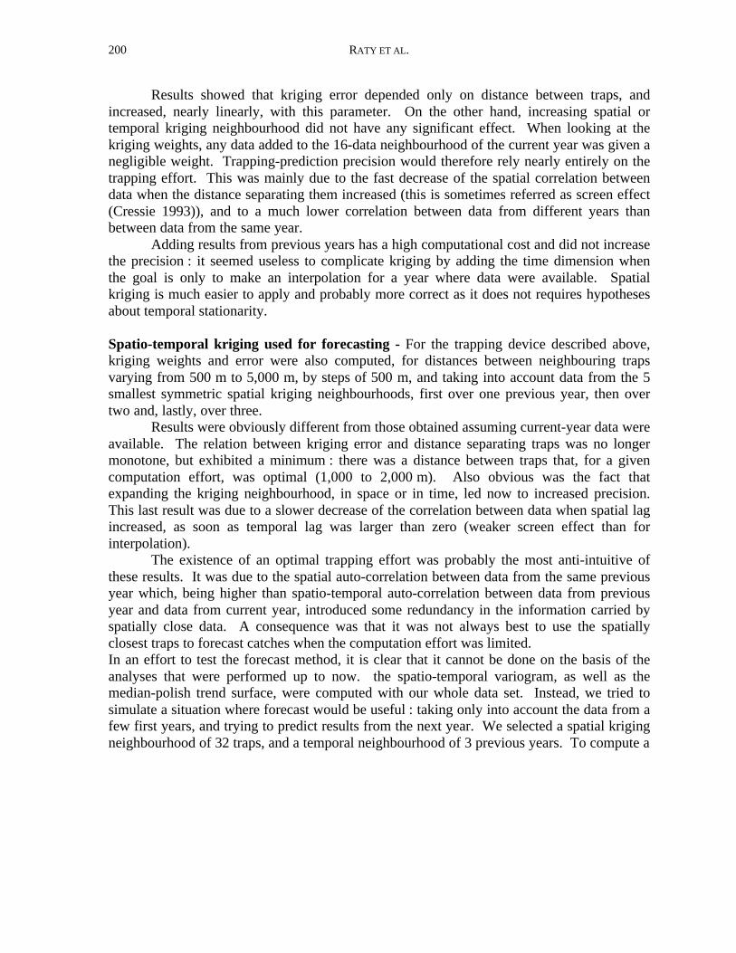
Results showed that kriging error depended only on distance between traps, andincreased, nearly linearly, with this parameter. On the other hand, increasing spatial ortemporal kriging neighbourhood did not have any significant effect. When looking at thekriging weights, any data added to the 16-data neighbourhood of the current year was given anegligible weight. Trapping-prediction precision would therefore rely nearly entirely on thetrapping effort. This was mainly due to the fast decrease of the spatial correlation betweendata when the distance separating them increased (this is sometimes referred as screen effect(Cressie 1993)), and to a much lower correlation between data from different years thanbetween data from the same year.

Adding results from previous years has a high computational cost and did not increasethe precision : it seemed useless to complicate kriging by adding the time dimension whenthe goal is only to make an interpolation for a year where data were available. Spatialkriging is much easier to apply and probably more correct as it does not requires hypothesesabout temporal stationarity.

Spatio-temporal kriging used for forecasting - For the trapping device described above,kriging weights and error were also computed, for distances between neighbouring trapsvarying from 500 m to 5,000 m, by steps of 500 m, and taking into account data from the 5smallest symmetric spatial kriging neighbourhoods, first over one previous year, then overtwo and, lastly, over three.

Results were obviously different from those obtained assuming current-year data wereavailable. The relation between kriging error and distance separating traps was no longermonotone, but exhibited a minimum : there was a distance between traps that, for a givencomputation effort, was optimal (1,000 to 2,000 m). Also obvious was the fact thatexpanding the kriging neighbourhood, in space or in time, led now to increased precision.This last result was due to a slower decrease of the correlation between data when spatial lagincreased, as soon as temporal lag was larger than zero (weaker screen effect than forinterpolation).

The existence of an optimal trapping effort was probably the most anti-intuitive ofthese results. It was due to the spatial auto-correlation between data from the same previousyear which, being higher than spatio-temporal auto-correlation between data from previousyear and data from current year, introduced some redundancy in the information carried byspatially close data. A consequence was that it was not always best to use the spatiallyclosest traps to forecast catches when the computation effort was limited.In an effort to test the forecast method, it is clear that it cannot be done on the basis of theanalyses that were performed up to now. the spatio-temporal variogram, as well as themedian-polish trend surface, were computed with our whole data set. Instead, we tried tosimulate a situation where forecast would be useful : taking only into account the data from afew first years, and trying to predict results from the next year. We selected a spatial krigingneighbourhood of 32 traps, and a temporal neighbourhood of 3 previous years. To compute a

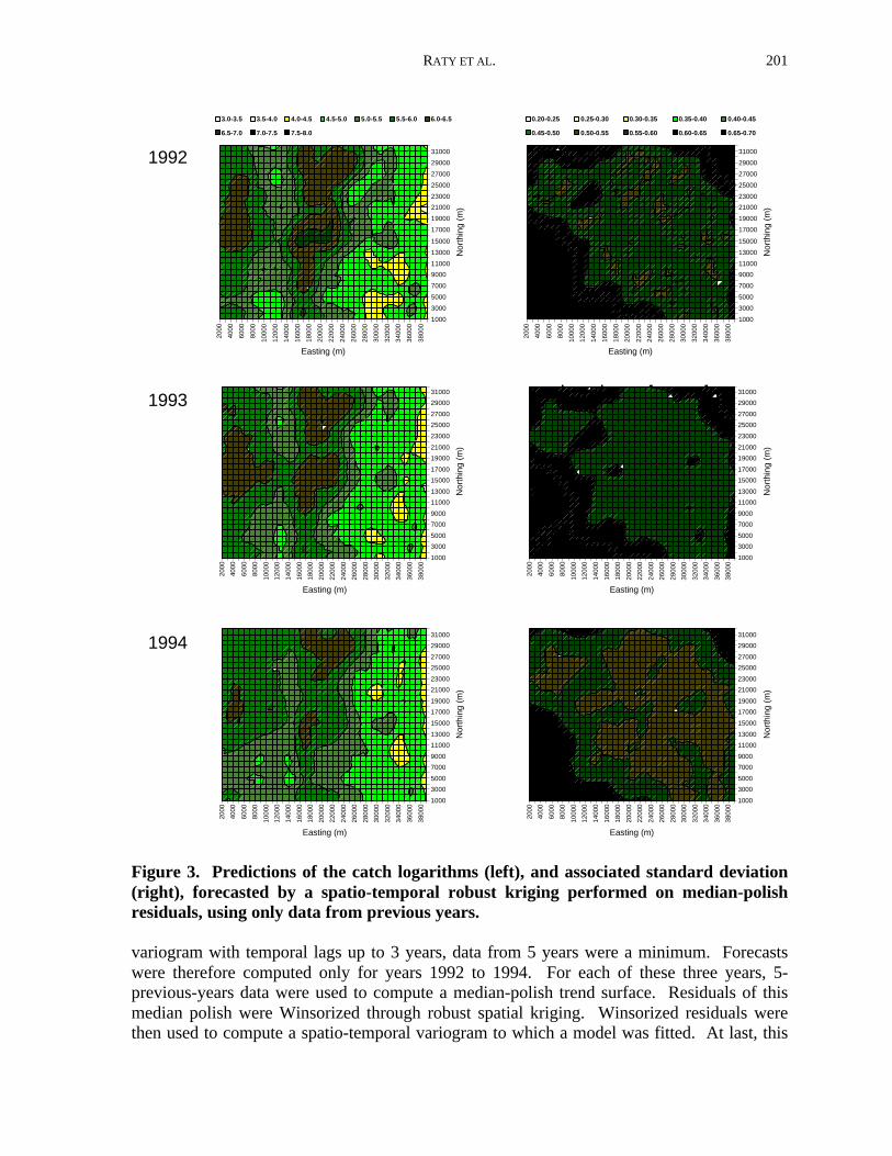
RATY ET AL. 201

1992

1993

1994

2000

4000

6000

8000

1000

0

1200

0

1400

0

1600

0

1800

0

2000

0

2200

0

2400

0

2600

0

2800

0

3000

0

3200

0

3400

0

3600

0

3800

0

1000

3000

5000

7000

9000

11000

13000

15000

17000

19000

21000

23000

25000

27000

29000

31000

Easting (m)

Nor

thin

g (m

)

3.0-3.5 3.5-4.0 4.0-4.5 4.5-5.0 5.0-5.5 5.5-6.0 6.0-6.5

6.5-7.0 7.0-7.5 7.5-8.0

2000

4000

6000

8000

1000

0

1200

0

1400

0

1600

0

1800

0

2000

0

2200

0

2400

0

2600

0

2800

0

3000

0

3200

0

3400

0

3600

0

3800

0

1000

3000

5000

7000

9000

11000

13000

15000

17000

19000

21000

23000

25000

27000

29000

31000

Easting (m)

Nor

thin

g (m

)

2000

4000

6000

8000

1000

0

1200

0

1400

0

1600

0

1800

0

2000

0

2200

0

2400

0

2600

0

2800

0

3000

0

3200

0

3400

0

3600

0

3800

0

1000

3000

5000

7000

9000

11000

13000

15000

17000

19000

21000

23000

25000

27000

29000

31000

Easting (m)

Nor

thin

g (m

)

2000

4000

6000

8000

1000

0

1200

0

1400

0

1600

0

1800

0

2000

0

2200

0

2400

0

2600

0

2800

0

3000

0

3200

0

3400

0

3600

0

3800

0

1000

3000

5000

7000

9000

11000

13000

15000

17000

19000

21000

23000

25000

27000

29000

31000

Easting (m)

Nor

thin

g (m

)

2000

4000

6000

8000

1000

0

1200

0

1400

0

1600

0

1800

0

2000

0

2200

0

2400

0

2600

0

2800

0

3000

0

3200

0

3400

0

3600

0

3800

0

1000

3000

5000

7000

9000

11000

13000

15000

17000

19000

21000

23000

25000

27000

29000

31000

Easting (m)

Nor

thin

g (m

)

2000

4000

6000

8000

1000

0

1200

0

1400

0

1600

0

1800

0

2000

0

2200

0

2400

0

2600

0

2800

0

3000

0

3200

0

3400

0

3600

0

3800

0

1000

3000

5000

7000

9000

11000

13000

15000

17000

19000

21000

23000

25000

27000

29000

31000

Easting (m)

Nor

thin

g (m

)

0.20-0.25 0.25-0.30 0.30-0.35 0.35-0.40 0.40-0.45

0.45-0.50 0.50-0.55 0.55-0.60 0.60-0.65 0.65-0.70

Figure 3. Predictions of the catch logarithms (left), and associated standard deviation(right), forecasted by a spatio-temporal robust kriging performed on median-polishresiduals, using only data from previous years.

variogram with temporal lags up to 3 years, data from 5 years were a minimum. Forecastswere therefore computed only for years 1992 to 1994. For each of these three years, 5-previous-years data were used to compute a median-polish trend surface. Residuals of thismedian polish were Winsorized through robust spatial kriging. Winsorized residuals werethen used to compute a spatio-temporal variogram to which a model was fitted. At last, this

RATY ET AL.202

model was used to compute predictions and prediction errors for the considered year, withdata from the 32 nearest traps and the 3 previous years. Results are mapped in Figure 3 andmay be compared to results of the robust spatial kriging performed on the data of these years(Figure 1). There was a good correspondence between the forecast prediction and the robustspatial kriging prediction. For 1992, 1993 and 1994, respectively 100%, 95.89% and 93.67%of the spatial robust kriging predictions fell within the 95% confidence interval associated tothe forecast prediction.

Conclusions

In conclusion, we think we showed that Ips typographus-monitoring trapping doesnot produce erratic results. On the contrary, results were highly structured, showing anapparently permanent mean structure and spatial as well as temporal continuity. Ouranalyses allowed us to build predictions of the logarithmic catch with an acceptable precisionwhen using the current-year data, and to forecast this logarithm, with less precision yet stillreliably.

It is important to stress that these analyses do not explain in any way the reasons ofcatch variations, they only describe them with mathematical tools. However, they might be agood beginning point to start other analyses. The median-polish trend surface, whichremains constant in time, might be tentatively correlated to permanent ecological factors(such as forest or soil characteristics, elevation, slope orientation, etc...). Departures fromforecast models might be correlated with more sudden events (such as windfall andsnowbreak occurrences).

It must also be stressed that these whole analyses were performed on basis of resultsproduced in an area where Ips typographus populations are endemic. In epidemic situation,results would have been probably much more erratic and less structured. Moreover, thetransition between endemic and epidemic situation in a bark-beetle population is probablynot a linear phenomenon. This transition might be described as departure from the linearmodel that we describe here.

Acknowledgements

This work was made possible by the establishment of scientific relations between theULB at Brussels and ICAS in Romania, that was helped by funding for international openingfrom the CGRI-DRI, and by the acquisition of computer hardware and software, from theFNRS-LN (grant F 5/4/85-OL-9.708). We also would like to thank the Romanian foresters,from ROMSYLVA, for collecting and producing the data that were the basis of this work.

RATY ET AL. 203

References Cited

Cressie, N. 1993. Statistics for spatial data, Revised Edition. Wiley Series in Probabilityand Statistics, Wiley, New York.

Cressie, N., and D.M. Hawkins. 1980. Robust estimation of the variogram. J. Intern.Assoc. Math. Geol. 12 : 115-125.

Hawkins, D.M., and N. Cressie. 1984. Robust kriging - A proposal. J. Intern. Assoc.Math. Geol. 16 : 3-18.

Hohn, M.E., A.M. Liebhold, and L. Gribko. 1993. Geostatistical Model for ForecastingSpatial Dynamics of Defoliation by the Gypsy Moth (Lep.: Lymantriidae). Environ.Entom. 22(5): 1066-1133.

Isaaks, E.H., and R.M. Srivastava. 1989. An introduction to applied geostatistics. OxfordUniversity Press.

Lieutier, F. 1990. Les réactions de défense du Pin sylvestre contre les attaques d’insectesscolytides, C.R. Acad. Agric. Fr. 76(4): 3-12.

Matheron, G. 1962. Traité de géostatistique appliquée, Tome 1. Mémoires du Bureau deRecherches Géologiques et Minières, N° 14. Editions Technip, Paris.

Raty, L., A. Drumont, N. De Windt, and J.C. Grégoire. 1995. Mass-trapping of thespruce bark beetle Ips typographus L.: traps or trap trees? For. Ecol. and Manag. 78:191-205.

Rossi E., D. Mulla, A. Journel, and E. Franz. 1992. Geostatistical tools for modelling andinterpreting ecological spatial dependence. Ecol. Mono. 62(2): 277-314

Tukey, J. 1977. Exploratory Data Analysis. Addison-Wesley, Reading, Massachusetts.

Speight, M.R. 1996. Host-tree stresses and the impact of insect attack in forest plantations.IUFRO Symposium, Kerala Forest Research Institute, Peechi, India. (in press).