spe 1578 pa boberg lantz
TRANSCRIPT
8/10/2019 SPE 1578 PA Boberg Lantz
http://slidepdf.com/reader/full/spe-1578-pa-boberg-lantz 1/11
Calculation of the Production
Rate of a Thermally Stimulated
Well
ABSTRACT
T
C BOBERG
R B LANTZ
JUNIOR
MEMBERS
AIME
This paper presents a
method
for calculating the pro
ducing rate
of
a well as a function
of
time following steam
stimulation. The calculations have proved valuable in both
selecting wells for stimulation alld
ill
determining
optimum
treatment sizes.
The
heat transfer
model
accounts for cooling
of
the oil
sand by both vertical alld radial conduction. Heat losses
for any
number
of productive sands separated by unpro
ductive rock are calculated for the injection. shut-in and
production phases
of
the cycle. The oil rate increase caused
by viscosity reduction due to heating is calculated by
steady-state radial flow equations. The response
of
Sllcces
sive cycles of steam injection call also he calculated with
this method.
Excellent agreement
is
shown betweell calculated and
actual field results. lso included are the results
of
several
reservoir
and
process variable studies. The method is best
suited for wells producing from a multiplicity
of
thin sands
where the bulk of the stimulated production comes from
the unheated reservoir. The flow equations used neglect
gravity drainage and sall/ration changes within the heated
region.
INTRODUCTION
This paper presents a calculation method which can be
used to predict the field performance
of
the cyclic steam
stimulation process.
The
calculation method enables the
engineer to select reservoirs that have favorable charac
teristics for steam stimulation and permits him to deter
mine how much steam must be injected to achieve fav
orable stimulation. While the calculation represents a con
siderable simplification
of
physical reality and the results
are subject to numerous assumptions which must be made
about the reservoir, it has been found that realistic calcu
lations
can
be made
of
individual well performance fol
lowing steam injection.
The
duration
of
the stimulation effect will depend pri
marily on the rate
at
which the heated oil sand cools which,
in turn,
is
determined
by
the rate at which energy
is
re
moved from the formation with the produced fluids and
conducted
from
the heated oil sand to unproductive rock.
A complete mathematical solution to this problem is a
formidable task,
and
finite difference techniques would un
doubtedly have
to
be used.
The
calculation method pre-
Original manuscript received
n
Society of Petroleum Engineers office
July 8, 1966. Revised manuscript received Oct. 31, .1966. a ~ e r SPE
1578)
was presented
a t SPE
41st
Annual Fall Meetmg
held
m
Dallas.
Tex., Oct. 2-5, 1966.
©
Copyright 1966 American
Institute
of Mining,
Metallurgical,
and Petroleum Engineers, Inc.
DECEMBER 966
ESSO
PRODUCTION
RESEARCH
CO.
HOUSTON
TEX
sented here utilizes analytic solutions
of
simple related
heat transfer and fluid flow problems.
The
method is suf
ficiently simplified that it can be used as a hand calcula
tion, although the calculations are somewhat lengthy and
laborious.
For
that reason, the analysis was programmed
for an IBM 7044 digital computer.
Well responses observed at the Quiriquire field in east
ern Venezuela have been matched using this program after
making suitable approximations for reservoir and well bore
conditions. One
of
the most valuable uses
of
this calcu
lation method
is
to assess the effect
of
reservoir and proc
cess variables on the stimulation response. This paper con
tains results of several studies made
of
key reservoir and
process parameters. Among the most important
of
these is
the influence
of
prior well bore permeability damage. I f a
well
is
severely damaged prior to stimulation, a higher
stimulation response will be observed than
if it
is undam
aged. I f a portion
of
this damage
is
removed. a permanent
rate improvement will occur.
THEORY
DESCRIPTION OF
CALCULATION
METHOD
The
process of cyclic steam stimulation
is
essentially one
of reducing oil viscosity around the well bore by heating
for a limited distance out into the formation through the
injection
of
steam. Suitable modifications
of
the calculation
technique presented here can be made so
that
stimula
tion of wells by hot gas injection
or
in situ combustion can
also be calculated.
A schematic drawing
of
the heat transfer and fluid flow
considerations included in the calculation method is shown
in Fig. 1
In
brief, the calculation assumes that the oil sand
is
uniformly and radially invaded by injected steam. For
wells producing from several sands, each sand
is
assumed
to be invaded to the same distance radially.
In
calculating
the radius heated r
h
energy losses from the wellbore and
conduction to impermeable rock adjacent
to
the producing
sands are taken into account. After steam injection is
stopped, heat conduction continues and oil sands with r
<
r
cool as previously unheated shale and oil sand at
r r
h
begin to warm.
The
effect
of
warming of oil sand
out
beyond
1'
has little effect on the oil production rate
compared to the effect
of
cooling
of
the oil sand nearer the
wellbore than r o Thus, in computing the oil production
rate, an idealized step function temperature distribution in
the reservoir is assumed where the original temperature
exists for r
> r
and where an average elevated tempera
ture exists for r r o
The
average temperature in the oil
sand for the region r
1'
is computed as a function
of
_ _
9References
given
a t end of paper.
1613

8/10/2019 SPE 1578 PA Boberg Lantz
http://slidepdf.com/reader/full/spe-1578-pa-boberg-lantz 2/11
time following termination of steam injection by an energy
balance.
From
the average temperature, the oil viscosity in
this region is determined.
The
oil production rate is calcu
lated by a steady-state radial flow approximation which
accounts for the reduced oil viscosity in this region.
SIZE O F T H E H E A T E D REGIO . ;
Wellbore Heat Losses
To
calculate the size
of
the region heated by steam, it
is necessary to estimate the quantity of heat actually in
jected af ter well bore heat losses are taken into account .
Various methods are available for estimating wellbore heat
losses.
0,11
A simple method which assumes a constant, aver
age temperature
of
the injected steam and an average
initial geothermal gradient computes the cumulative energy
lost during injection Q" as:
.(
aD)
2r.DKr,
T T
r
2 I
Q -
a
(1)
where
I
is read from Fig. 2 as a function of dimensionless
time
at, 1
1', .
For
uninsulated tubing or the case where steam
is in direct contact with the casing wall, r, is the inside
FLOW OF OIL
WATER
G S
. /VVVv
HE T
CONDUCTION
OIL
S ND
SH LE
OIL SAND
SH LE
OIL SAND
FIG.
I-SCHEMATIC REPRESE] o;TATlOl i
OF HEAT TRANSFER
Al iD
FLUID
FLOW CALCULATED BY
MATHEMATICAL MODEL.
10
F
====:::;... :
FIG.
2-1 FACTOR FOR WELLBORE HEAT Loss DETERMINATION.
1 6 1 4
casing radius; for insulated tubing.
1',
may be roughly ap
proximated as the inside tubing radius.
The
average down-hole steam quality X for the entire
steam injection period is then
X, =
X 'f - MQ'J
.
,
If,
2)
Heated Radills
During steam injection the oil sand near the well bore
is at condensing steam temperature
L.
the temperature
of
saturated steam at the sand face injection pressure.
Pressure fall-off away from the well during injection is
neglected in this analysis. and T, is assumed to exist out
to a distance
r o
where the temperature falls sharply to
Tr,
the original reservoir temperature.
In
reality, the tem
perature falls more gradually to reservoir temperature be
cause of the presence of the hot water bank ahead of the
steam,
but
this is neglected to simplify the calculation.
The heated zone radius is calculated by the equation of
Marx and Langenheim: In the case
of
multisand reser
voirs, if it is assumed that each sand is invaded uniformly
as
though all sands had the same thickness
h
and were in
vaded by equal amounts
of
steam:
r.'
=
hM. (XiII , + h, - /z .) f, .
4Kr.(T, - T,.)t,N,
(3)
The
function
l.
is plotted as a function
of
dimension
less time T
=
4Kt, h'(pC)] in Fig. 3.
The
use of·this equa
tion for multisand reservoirs also assumes that injection
times are sufficiently short and that interbedded shale is
sufficiently thick that no heating occurs
at
the mid-plane
of the shale during the injection period. Eq. 3 further as
sumes that the value
of average density times heat ca
pacity pC for the barren strata is the same as that for the
oil sands
[(pC),h
Ie
= (pC),].
For
multisand reservoirs, a heated radius for each sand
r i could be calculated assuming equal steam injection
per
foot
of
net sand. An average heated radius
rh
could then
be computed from rio
= h,r,,,'/ h,.
Practically speaking.
the r' for reservoirs consisting of more than three sands
of
reasonably uniform thickness can be approximated by
using Eq.
3.
T E M P E R A T U R E H I S TO R Y O F
T H E
H E A T E D R E G I O N (r ,
<
r
<
r.)
The average temperature Tav.
of
the heated region (or
I O r ~
t
~ - - -
0.01
; ; ; - - - - - ~ - - _ ; : _ : - - - - - - - - _ _ : _ _ = _ - - - - - ~ ~ - - - - - - - - ~
0.01
0.1
1.0 10
FIG.
3--DIMENSIONLESS
PUSITlOl i OF STEAMI:D·OUT REGION.
JO t T R 'i A L O F P E T R O L E U M T E C H l O L O ( ; Y
8/10/2019 SPE 1578 PA Boberg Lantz
http://slidepdf.com/reader/full/spe-1578-pa-boberg-lantz 3/11
regions in the case of a multisand reservoir)
after
termina
tion of steam injection is calculated from an approximate
energy balance
around
the region r <
I'
<
r
h
:
T,,
= T,
+
(T, - T..)
[ v ~
(1 - 8) - 0],
OF
4)
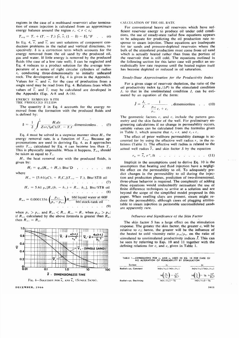
In Eq. 4, and ~ are unit solutions of component con
duction problems in the radial and vertical directions, re
spectively. 8 is a correction term which accounts for the
energy removed from the oil sand by the produced oil,
gas and water. I f little energy is removed by the produced
fluids (the case of a low rate well), 8
can
be neglected and
Eq. 4 reduces to a product solution for the average tem
perature of
a series of right circular cylinders of radius
r conducting three-dimensionally to initially unheated
rock. The development of Eq. 4 is given in the Appendix.
Values for
V,'
and ;;-, for the case of production from a
single sand may be read
from
Fig.
4.
Relations
from
which
values of
y,
and
Y may
be calculated are developed in
the Appendix (Eqs. A-8 and A-16).
ENERGY REMo\ED \\ITH
THE PRODUCED FLums
The quantity 8 in Eq. 4 accounts for the energy re
moved from the formation with the produced fluids and
is defined by:
I
If
Hfdx
=
2 ZTrr,,'(pC),(L _
T..)' dlll1enslOnless .
(5)
I,
Eq. 4 must be solved in
a
stepwise
manner
since
H
the
energy removal rate, is a function of T g. Because ap
proximations are used in deriving Eq. 4, as 8 approaches
unity
1',,,
calculated by Eq. 4 can hecome less than
T,
.
This is physically impossible. When it happens, T,, should
be taken as equal to
T,.
H the
heat
removal rate with the produced fluids, is
given by:
H
f
=
q (H..,,
+
H,,),
Btu/D
(6)
where
H
= [5.61(pC) +
R c ](T,, -
T,.),
Btu/STB oil
(7)
H = 5.61
p,,[R,,(/lr
- h
r
,. + R ,. h
f
. , ] , Btu/STB oil
(8)
wv • 1356 . . ,
=
0000
(P )R
bblliquid water
at
60F
£I
...
-
P ..
·
bbl stock-tank 011
(9)
when
P
>
p .. . and R .1' < R ... , R ... . = R when p ,
>
p,,;
if
R .,
calculated by the above formula is greater than
R,,,
then
R .,
=
R .
1.0
;:::-
0,8
0.6
0.4
0.2
o
0.01
r--.
~ I I I Il( -
tj
l
IIIII
I I
III
41l(t-t
j
)
.........,
Vr: 8= - - 2 -
V
: 8 = - - - 2 -
rh
IIIII
I
r
-
I
'-
VZ - I I ~ I ~ G L ~
~ A I ~ ~
,-
Vr
I
'
-.....
.......
0.1
1.0
10
10C
8 - DIMENSIONLESS TIME
FIG.
4- -S0LUTION FOR
;;r AN[);;z (SINGLE
SA;,\[).
DEeEMI lER,
1966
C L C U L T l O ~ OF
THE OIL
RATE
For conventional heavy oil reservoirs which have suf
ficient reservoir energy to produce oil under cold condi
tions, the use of steady-state radial flow equations appears
to be adequate for predicting the oil production rate re
sponse to steam injection.
These
equations are inadequate
for tar sands and pressure-depleted reservoirs where the
bulk of the stimulated production must come from oil sand
which is actually heated
rather
than from the portion
of
the reservoir that is still cold. The equations outlined in
the following section for this latter case will predict an un
realistically low rate response until the heated region itself
has become depleted or reduced in oil saturation.
Steady-State
A pproxill1ation
for
the Productivity
Index
For a given stage of reservoir depletion, the ratio
of
the
oil productivity index
(q,J
6..P) in the stimulated condition
i to that in the unstimulated condition
J
e
can be esti
mated by an equation of the form:
- _ i _ 1
-
J,
, dimensionless
(10)
{t c,
+
c,
p.,,,
The
geometric factors c, and c, include the pattern geo
metry and the skin factor of the well. For preliminary en
gineering calculations if no change in permeability occurs,
suitable values can be calculated from the formulas given
in Table I, which assume that r
« r,
and r r «
r,.
The effect of prior wellbore permeability damage is ac
counted for by using the effective well radius r in the re
lations (Table 1).
The
effective well radius is related to the
actual well radius r and skin factor S by the equation
(11)
Implicit in the assumptions used to derive Eq. 10 is the
assumption
that
heating and fluid injection have a negligi
ble effect on the permeability to oil.
To
adequately pre
dict changes in the permeability to oil during the injec
tion and production phases, prediction
of
two-dimensional,
three-phase behavior is required. The complexity of adding
these equations would undoubtedly necessitate the use
of
finite difference techniques to arrive at a solution
and
are
beyond the scope
of
the simplified model proposed in this
paper. When swelling clays are present, steam might re
duce the permeability, although cases
of
plugging attribu
table to steam injection in permeable unconsolidated sands
are apparently rare.
Influence and
Significance
of the Skin Factor
The
skin factor S has a large effect
on
the stimulation
response. The greater the skin factor, the greater c, will be
relative to
c,;
hence, the greater will be
the
influence of
the heated to cold viscosity ratio {tu'./P-., on the
ratio
of
stimulated to unstimulated productivity indices I. This can
be seen by referring to Eqs. 10 and 11 together with
the
defining relations for
c,
and
c,
given in Table
1.
TABLE
I-EXPRESSIONS FOR c, AND c, USED IN
EQ. 10
FOR
CASE
OF
NO
ALTERATION
OF
PERMEABILITY
BY
STIMULATION
System
c,
Radial-Pe onstant I (rhl rw J/ In(r,,/r Ie)
I (rhl
TtIJ
)/ ln(re/ru:)
(
'I, )
'I,'
In -
--
r
U'
2r,--
) ,
n - - V, - .
Th
2
re
:J
Radial-pi Declining
In ( I , · ) - 'h
1615
8/10/2019 SPE 1578 PA Boberg Lantz
http://slidepdf.com/reader/full/spe-1578-pa-boberg-lantz 4/11
Another
way
to
understand the effect of S is to consider
k,j
and
rd, the permeability and radius
the region
around
the well bore where permeability
k:
(
k ) r
S =
k J
In-=-.
d rtl
12)
f
kd
is small relative to k and
r
> r ., then
S
will have a
Alteration oj Skin Factor hy Heating
In some wells asphaltene precipitation may be a cause
of
f this
and
similar damage can be allevi
by
heating, suitable modification
of c,
and c, can be
For
the
constant p, case where the skin factor S is re
to S,
following stimulation
and
r
> rd:
c, =
S, +
In rh/r .
S + In
relr ,
(13)
1n
r,/r
h
;
c: =
S
+
In
rJf ,
p, is de
Determination
of the Oil RaIl'
To
obtain the oil rate as a function of time.
It IS
neces
to
know the unstimulated productivity index J, and
p,
as a function of the cumu
Then
the stimulated oil rate q h
qoh = J J,. : P. STB/D
14)
T is determined from Eq. 10;
J,
is obtained from
extrapolated plot of the productivity index history of
prior
to stimulation; and : P the pressure draw
Pe
- p ,
during the period
of
stimulated produc
The
static pressure p,
can
be estimated from an extra
of a plot of p, vs cumulative oil produced prior
enance benefits of the injected fluids can be neglected.
PERFORMANCE
SUCCEEDING CYCLES
To calculate the performance
of
cycles following the
made
for the residual heat left in
The
energy remain
by:
Heat
remaining =
u,,'(pC)J1N,
(T,,, -
T,.)
(15)
An
approximate method
of
taking this energy into ac
is to add it
to that
injected during the succeeding
that
injection takes place into a res
that
is at original temperature
T,.
This additional
The major
assumption involved in this approximation is
at
the beginning
of
is a conservative assumption since calcu
heat
losses for cycles after the first will be higher
han
those actually observed. A more optimistic analysis
ould assume
that
all of the energy remaining, including
in
the
shale,
is
added to the energy injected
on
the suc
TABLE 2-STEAM STIMULATION TEST DATA FOR WelL
Q-594
Reservoir Characteristics
Depth. It
Section thickness ft
Net
sand thickness ft
Number of
sands
Oil
viscosity. cp
Pre-stimulation
Oil
rate, BID
WOR, bbl/bbl
GOR, scflbbl
Stimulation
Steam injected MM b
Wellhead inie ctio n pressure psig
Injection time including
shut-in
days
Durat ion of cycle including
injection
days
Stimulated
producing
time. days
Actual oil production bbl
Calculated oil
production
bbl
Estimated
cold
production bbl
RESULTS
First
Cycle
18.1
770
46
487
378
80,803
79,140
47,600
MATCH OF FIELD
TEST
PERFORMANCE
WITH CALCULATIONS
4,050
470
183
16
133
135
0.83
985
Second Cycle
19.2
800
55
354
288
47,813
53,700
30,400
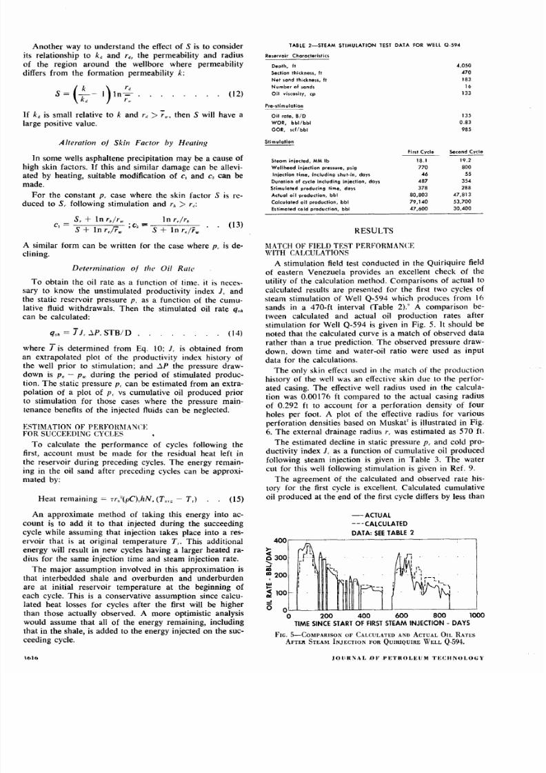
A stimulation field test conducted in the Quiriquire field
of eastern Venezuela provides an excellent check
of
the
utility of the calculation method. Comparisons of actual to
calculated results are presented for the first two cycles of
steam stimulation
of
Well Q-594 which produces from 16
sands in a 470-ft interval (Table
2).
A comparison be
tween calculated and actual oil production rates after
stimulation for Well Q-594 is given in Fig. 5. It should be
noted that the calculated curve is a match of observed data
rather than a true prediction. The observed pressure draw
down. down time and water-oil ratio were used as input
data for the calculations.
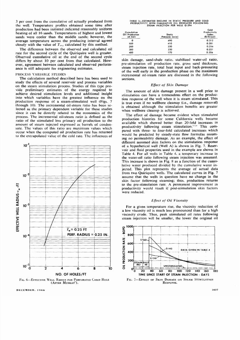
The only skin effect used in the match of the production
history of the well was an effective skin due to the perfor
ated casing. The effective well radius used in the calcula
tion was 0.00176 ft compared to the actual casing radius
of 0.292 ft to account for a perforation density of four
holes per foot. A plot
of
the effective radius for various
perforation densities based on Muska ' is illustrated in Fig.
6. The
external drainage radius
r,
was estimated as 570 ft.
The
estimated decline in static pressure p, and cold pro
ductivity index
J
as a function of cumulative oil produced
following steam injection is given in Table 3.
The
water
cut for this well following stimulation is given in Ref. 9.
The agreement of the calculated and observed rate his
tory for the first cycle is excellent. Calculated cumulative
oil produced at the end
of
the first cycle differs by less than
-ACTUAL
---CALCULATED
DATA: SEE
TABLE
2
400 ----------------------------------
>-
300
III
: 100-
5
OLi
__
~ _ i l W l l
__
__________
__
o 200 400 600 800 1000
TIME
SINCE
START
OF
FIRST STEAM INJECTION -
DAYS
FIG. 5-C0Il1PARISOl \
OF CALCULATED AND ACTUAL OIL RATES
AFTEft STEAII1
INJECTlOl \
FOR
QUlRIQUlRE WELL
Q-594.
JO l iR : \A L o F P E T I IO L E U M
TECHl \Ol .OGY
8/10/2019 SPE 1578 PA Boberg Lantz
http://slidepdf.com/reader/full/spe-1578-pa-boberg-lantz 5/11
3 per cent from the cumulative oil actually produced from
the well. Temperature profiles obtained some time after
production had been initiated indicated reasonably uniform
heating of all 16 sands. Temperatures of highest and lowest
sands were cooler than the middle sands; however, the
average temperature across the producing interval agreed
closely with the value of T,,, calculated by this method.
The
difference between the observed and calculated oil
rate for the second cycle of the Quiriquire well is greater.
Observed cumulative oil
at
the end of the second cycle
differs by about 10 per cent from that calculated. How
ever, agreement between calculated and observed perform
ance is still adequate for engineering estimates.
P R O C E S S
Y
A R I A B L E S T U D I E S
The calculation method described here has been used to
study the effects of several reservoir and process variables
on the steam stimulation process. Studies of this type pro
vide preliminary estimates
of
the energy required to
achieve desired stimulation levels and additional insight
into which variables have the greatest influence on the
production response of a steam-stimulated well (Figs . 7
through 10).
The
incremental oil-steam ratio has been se
lected as the primary dependent variable for these studies
since it can be directly related to the economics
of
the
process. The incremental oil-steam ratio is defined as the
ratio of the stimulated less primary oil production to the
amount of steam injected expressed as barrels of conden
sate.
The
values
of
this ratio are maximum values which
occur when the computed oil production rate has returned
to the extrapolated value
of
the cold rate. The influences of
I-
...
...
I
V I
::::>
o
ct
ar::
IO-J
-
-
w
~
w
>
~
u
w
...
w
,
_.-
_.
-
I
- - - + ~ ~ - - + -
/
/
i
:
/
/
/
:
/
I
I
~ - -
I
[7
I
/
,
- -
/
/
,
/
,
1 1
T
rw= 0.25 FT
I
PERF. RADIUS
=0.25
IN.
-_ .
I
-- ---
i
,
i
_-_._
I
T
I
i
i i
2
4
6
8
10
NO.
OF
HOlES/FT
FIG. 6--EFFECTIVE \VELL
RADIUS
FOR PERFORATED CASED HOLE
(AFTER
MUSKAT ).
D E C E M I I E I I 1 9 6 6
TABLE
3-ESTIMATED DECLINE IN STATIC
PRESSURE
AND COLD
PRODUCTIVITY WITH CUMULATIVE
OIL PRODUCED
FOLLOWING
STEAM
INJECTION fOR WELL
Q·59
Cold
Cumulative
Productivity
Ojl Production Static Index
M bbl) Pressure psio) B/D/psi)
0
490 0.312
100
410
0.281
200
330
0.256
300
250
0.231
400
170
0.206
skin damage, sand-shale ratio, stabilized water-oil ratio,
pre-stimulation oil production rate, gross sand thickness,
steam injection rate, total heat input and back-pressuring
of the well early in the production phase on the maximum
incremental oil-steam ratio are discussed
in
the following
sections.
Effect of kin Damage
The amount of skin damage present in a well prior to
stimulation can have a tremendous effect on the produc
tion response of the well when it is steam stimulated. This
is
true even if no well bore c leanup (i.e., damage removal)
is obtained although the stimulation benefits are greater
when well bore cleanup
is
achieved.
The effect of damage became evident when stimulated
production histories for some California wells became
available which showed better than 20-fold increases in
productivity following steam stimulation."'" This com
pared with three- to four-fold calculated increases which
would be predicted by steady-state flow formulas assum
ing no permeability damage. As an example, the effect of
different assumed skin factors on the stimulation response
of a hypothetical well (Well A) is shown in Fig. 7. Reser
voir and fluid properties used in the example are shown in
Table
4.
For all wells
in
Table
4,
a temporary increase
in
the water-oil ratio following steam injection was assumed.
This increase is shown in Fig. 8 as a function of the cumu
lative water produced divided by the cumulative water in
jected. This plot represents the average of actual data
from two Quiriquire wells. The calculated curves in Fig. 7
assume that the wells in question have no change in the
skin factor following steaming; thus, production returns
to the pre-stimulation rate. A permanent improvement
in
productivity would result if post-stimulation skin factors
were reduced.
Effect of Oil Viscosity
For a given temperature rise, the viscosity reduction of
a low viscosity oil is much less pronounced than for a high
viscosity crude. Thus, peak stimulated oil rates following
steam injection will be smaller, the lower the original oil
o l O O O r - - - , - - - , - - - , - - - - , - - - , - - - , - - - ,- - - - , - - ,
o
8 0 0 r - - - - - + - - - + - - - + - - - - ~ - -+--+-- - .+-
i
6 0 0 r - - - - + - - 1 - + - < - - + - - ~ - - - + - - - - L - - ~ - ..
- · -
z
o
5 4 0 0 f - - - + - - + + - ~ '
;:
o
o
,
DATA GIVEN IN
TABLE
4
'
....
2 0 0 r - - - - - ~ - - - ~ - - ~ - - ~ ~ ~ - - -
STEAM ' ~ ; ; ; ; ; ; ; ; ; ; ; ; ; ; ; ; : ; : ; : : : : : d
INJ
i
5
FIG. 7-EFFECT OF SKIN DAMAGE ON STEAM STIMULATION
RESPONSE.
1617
8/10/2019 SPE 1578 PA Boberg Lantz
http://slidepdf.com/reader/full/spe-1578-pa-boberg-lantz 6/11
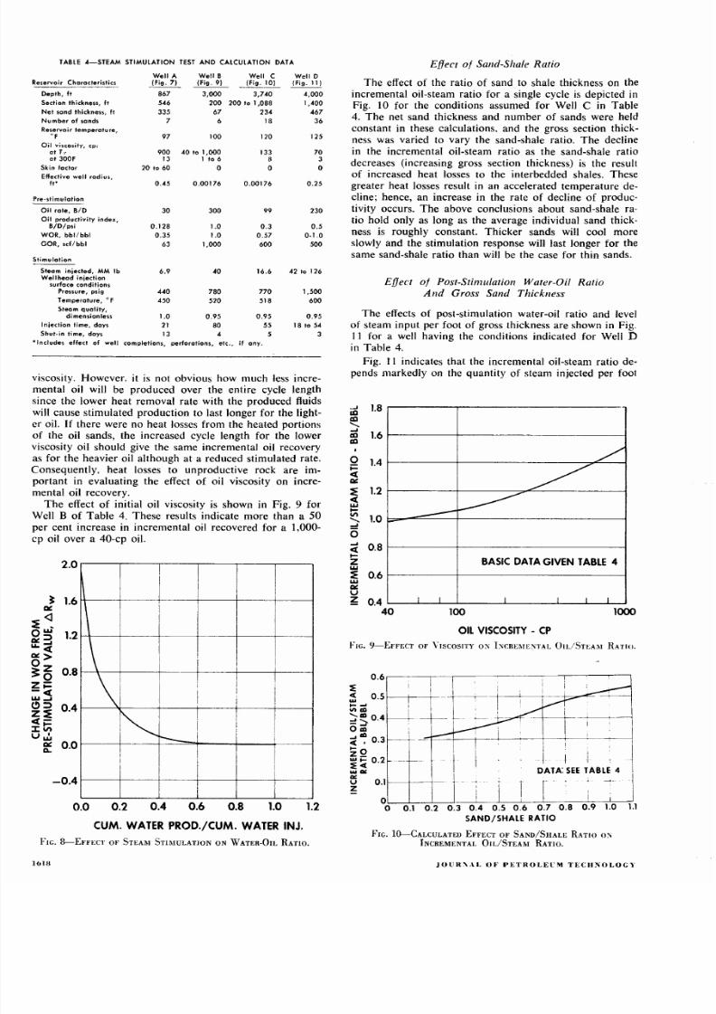
TABLE 4-STEAM STIMULATION
TEST
AND CALCULATION DATA
Reservoir Characteristics
Depth,
It
Section thickness,
ft
Net sand
thickness, ft
Number
of
sands
Reservoir temperature
of
Oil
viscosity,
cp:
at TI
at 300F
Skin
factor
Effective well
radius
ft
Pre-stimulation
Oil role,
BID
Oil productivity index,
B/D/psi
WOR, bbl/bbl
GOR, scf/bbl
Stimulation
Steam injected MM Ib
Wel lhead
injection
surface conditions
Pressure, psig
Well
A
(Fig. 7)
867
546
335
7
97
900
13
20
to
60
0.45
30
0.128
0.35
63
6.9
440
Well B
(Fig. 9)
3,000
Well C
(Fig. 10)
3,740
200
200 to
1 ,088
67
234
6
100
4010 1,000
1 to 6
o
0.00176
300
1.0
1.0
1,000
40
780
18
120
133
8
o
0.00176
99
0.3
0.57
600
16.6
770
Temperature, of
450 520 518
Steam
quality,
dimensionless
1.0 0.95
0.95
Injection
time, days 21 80 55
Shut-in time, days 13 4 5
*Includes effect of
well
completions, perforations, etc., jf any.
Well D
(Fig. 11)
4,000
1,400
467
36
125
70
3
o
0.25
230
0.5
0-1.0
s
42 to 126
1,500
600
0.95
18 to 54
3
viscosity. However, it
is
not obvious how much less incre
mental oil will be produced over the entire cycle length
since the lower heat removal rate with the produced fluids
will cause stimulated production to last longer for the light
er oil. I f there were no heat losses from the heated portions
of
the oil sands, the increased cycle length
for
the lower
viscosity oil should give the same incremental oil recovery
as for the heavier oil although at a reduced stimulated rate.
onsequently, heat losses to unproductive rock are im
portant
in evaluating the effect
of
oil viscosity
on
incre
mental oil recovery.
The
effect
of
initial oil viscosity is shown in Fig. 9 for
Well B of Table 4. These results indicate more than a 50
per
cent increase in incremental oil recovered for a 1,000-
cp oil over a 40-cp oil.
2.0
1.6
CI:
~ <
w
1.2
I:::l
..:c
I :>
z
0.8
~
-c(
W-A
C): : l
0.4
~
c(-
I:ti
uJJ
CI:
0.0
0..
I
I
I
I
\
I
I
I
i
i
I
\'
1
i
I
I
i
1
I
I
1
i
~
,
I
1
i
r--
I
I
1
I
I
I
I
i
i
I
-0.4
I
I
I
0.0
0.2
0.4 0.6 0.8 1.0
1.2
CUM.
WATER
PROD.jCUM.
WATER
INJ.
FIG. 8--EFFLCT
OF
STEAM STIMULATION ON WATER-OIL RATIO.
16111
Effect
of
Sand Shale Ratio
The effect of the ratio
of
sand to shale thickness on the
incremental oil-steam ratio for a single cycle
is
depicted
in
Fig. 10 for the conditions assumed for Well C in Table
4.
The
net sand thickness and number
of
sands were held
constant in these calculations. and the gross section thick
ness was varied to vary the sand-shale ratio. The decline
in the incremental oil-steam ratio as the sand-shale ratio
decreases (increasing gross section thickness)
is
the result
of
increased heat losses to the interbedded shales. These
greater heat losses result
in
an accelerated temperature de
cline; hence, an increase in the rate of decline of produc
tivity occurs. The above conclusions about sand-shale ra
tio hold only as long as the average individual sand thick·
ness is roughly constant. Thicker sands will cool more
slowly and the stimulation response will last longer for the
same sand-shale ratio than will be the case for thin sands.
Effect of Post Stimulation Water Oil Ratio
nd
Gross
Sand
Thickness
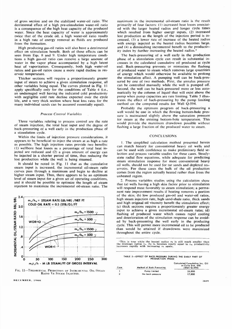
The
effects
of
post-stimulation water-oil ratio and level
of steam input per foot
of
gross thickness are shown in Fig.
11 for a well having the conditions indicated for Well D
in Table 4.
Fig. 11 indicates that the incremental oil-steam ratio de
pends markedly on the quantity
of
steam injected
per
foot
1 8
c:a
.....
~ 1.6
g
1.4
«
CI:
:E 1.2
«
t
' -
1.0
.....
o
4
0.8
Z
:E 0.6
CI:
U
~ 0.4
40
BASIC
DATA
GIVEN TABLE 4
I
1
1.
.1 .1
J.
100
1000
OIL
VISCOSITY - CP
FIG.
9 EFFECT
OF VISCOSITY 0:\
bCREMENTAL O I L / S T E A ~ 1
RATIO.
~
0.5
-
" 'a l
~ ~ 0 4
Oal
0.3
" ' 0
i=
0 2
~
« .
... co:
co:
I
-T- - t - - ' -
I
- --
L
; ~
- 1 1 F - - - + - - t - - - - + - ~ _ _ _ _ t _ _ - ~ - ~
DATA: m
~ B l ~
4
l
u 0.1
f--i-----j
z
FIG.
100CALCULATEU EFFECT
OF
SANU/SHALE RATIO 0:\
INCREMENTAL OIL/STEAM
RATIO.
JOl l IC\AL OF
I 'ETI tOLEl · \ t
T E C H N O L O G \ '
8/10/2019 SPE 1578 PA Boberg Lantz
http://slidepdf.com/reader/full/spe-1578-pa-boberg-lantz 7/11
of gross section and on the stabilized water-oil ratio. The
detrimental effect
of
a high pre-stimulation water-oil ratio
is a consequence
of
the high heat capacity
of
the produced
water. Since the
heat
capacity
of
water
is
approximately
twice that
of
the crude oil. a high water-oil ratio results
in a high rate of energy removal as fluids are produced
from the formation.
High producing gas-oil ratios will also have a detrimental
effect on stimulation benefit. Both
of
these effects can be
seen from Eqs. 8 and 9 Under high temperature condi
tions a high gas-oil ratio can remove a large amount of
water in the vapor phase accompanied by a high latent
heat
of
vaporization. Consequently, both high water-oil
ratios and gas-oil ratios cause a more rapid decline in res
ervoir temperature.
Thicker
sections will require a proportionately greater
input
of
steam to achieve a given stimulation response, all
other
variables being equal.
The
curves plotted in Fig.
11
apply specifically only for the conditions of Table 4 (i.e.,
an
undamaged well having the indicated cold productivity
with negligible cold rate decline expected over the cycle
life, and a very thick section where heat loss rates for the
many individual sands can be assumed essentially equal).
Process COlltrol Variables
Three
variables relating to process control are the rate
of
steam injection, the total heat input and the degree
of
back-pressuring
of
a well early in the production phase of
a stimulation cycle.
Within the limits of
injection pressure considerations,
it
appears to be beneficial to inject the steam at as high a rate
as possible. The high injection rates provide two benefits:
(1) well bore heat losses as a percentage
of
total heat in
jected
are
reduced and (2) a given amount
of
energy can
be injected in a shorter period
of
time, thus reducing the
lost production while the well is being steamed.
It should be noted in Fig.
11 that
as the cumulative
steam input is increased, the incremental oil-steam ratio
curves pass through a maximum and begin to decline at
higher steam input. Thus, there appears to be an optimum
level
of
steam
input
for a given set
of
operating conditions,
and it should be possible to optimize the length
of
steam
injection to maximize the incremental oil-steam ratio.
The
- 2.4
CD
CD
-
CD
2.0
CD
0
i=
1.6
I:
IX
<I:
1.2
on
-
5
S
-
<I:
Z
IX
U
0
0
ms/hn
=
STEAM RATE LB/HR) /NET FT
COLD OIL RATE = .5 STB/D)/FT
- - ---
,
m
s
/h
n
=1500
m
s
/h
n
=1500
ms/h
n
= 500
t
I
I
50
100
150
200
250
300
mst;/h
- M
LB
STEAM/FT
OF GROSS
INTERVAL
FIG. I I -THEORETICAL PREDICTlO'i OF I l 'iCRDIE'iTAI. O l J j S T E ~ I
RATIO \ 5 STEA \OI }l'iJECTED.
UE( ;E I I I IER.
1 9 6 6
maximum in the incremental oil-steam ratio is the result
primarily of four factors:
(I)
increased heat losses associat
ed with the larger heated radius and longer cycle times
which resulted from higher energy inputs. (2) increased
lost production as the length
of
the injection period is in
creased, (3) a lower rate
of
increase
of
the heated radius
with energy injected as the heated radius becomes large.
and (4) a diminishing incremental benefit to the productiv
ity index by further increasing the heated radius. *
The
back-pressuring
of
a well early in the production
phase
of
a stimulation cycle can result in substantial in
creases in the calculated cumulative oil produced
at
cycle
end. Back-pressuring prevents
or
minimizes the flashing
of
produced water to steam which removes large quantities
of
energy which would otherwise be available to prolong
the stimulation effect. A pumping well can be back-pres
sured by one of two methods. First. the annulus pressure
can be controlled manually while the well
is pumped off.
Second, the well can be back-pressured more
or
less auto
matically by the column
of
liquid that will exist above the
pump when
pump
capacities are rate limiting. Table 5 illus
trates the effect of back-pressuring by the pump limiting
method on the computed results for Well Q-594.
Probably the optimum program
of
back-pressuring a
well
would be one in which the flowing bottom-hole pres
sure is maintained slightly above the saturation pressure
for steam at the existing bottom-hole temperature. This
would provide the maximum drawdown possible without
flashing a large fraction of the produced water to steam.
CONCLUSIONS
I.
The
simplified calculation method presented herein
can match history for conventional heavy oil wells and
can be used with confidence to make preliminary field se
lection and process variable studies for these cases. Steady
state radial flow equations, while adequate for predicting
steam stimulation response for most conventional heavy
oil wells, should not be used for tar sands and depleted res
ervoirs. For these cases the bulk
of
the oil production
comes from the region actually heated
rather
than from the
unheated region.
2 Process variables studies using the calculation show
that (a) wells having a high skin factor prior to stimulation
will respond most favorably to steam stimulation; a perma
nent rate improvement results if heating removes a portion
of the skin; (b) low produced gas-oil and water-oil ratios,
high steam injection rate, high sand-shale ratio, thick sands
and high original oil viscosity benefit the stimulation effect;
(c) thick sections require a proportionately greater energy
input to achieve a given incremental oil-steam ratio; (d)
flashing
of
produced water which causes rapid cooling
and deterioration
of
the stimulation response can be avoid
ed by back-pressuring the well early in the producing
cycle. This will permit more incremental oil to be produced
than would be attained if drawdowns were maximized
throughout the entire cycle.
'::This
is
true while
the heated radius
h is still
much smaller than
the drainage
radius
reo
As rh
becomes nearly equal
to rtJ productivity
increases
rapidly
with
increasing
it again.
Case
2
TABLE 5-EFFECT OF BACK·PRESSURE DURING THE
EARLY PART
OF
PRODUCT
ION
PHASE
Method of Back·Pressuring
Pump limited
No bock-pressure
Calculated Cumulative Inc.
Oil
ot Cycle End.
STB
Well Q·594)
35,000
17,000
1619
8/10/2019 SPE 1578 PA Boberg Lantz
http://slidepdf.com/reader/full/spe-1578-pa-boberg-lantz 8/11
NOMENCLATURE
a = geothermal gradient, °F/ft
b
= square root
of
dimensionless time for radial
temperature decay (Eq. A-5, dimensionless)
B,
=
constant appearing
in
Eq. A-14, ft
c
C,
= constants appearing in Eq. 10, dimensionless
(Table I)
C
=
average specific
heat
of
gas, over temperature
interval T,. to T , ,
Btul
scf, 0 F
c C.' = average specific heats
of
oil and water over
the temperature interval T to
T
. .
Btu/lb
of
,
D = depth of the producing formation, ft
h = average thickness of the individual sand mem_
bers, ft
hi = enthalpy of liquid water at
T,,,
above 32F.
Btu/lb
hi.
=
specific enthalpy
of
vaporization
of
water at
T
DV
, Btu/lb
hiT = specific enthalpy of liquid water at T Btu/lb
hIs =
specific enthalpy
of
liquid water at T
Btu/lb
h, = individual sand thicknesses, ft
h, = artificially increased sand thickness used in Eq.
A-14, ft
HI
= rate at which energy is removed from the for
mation with the produced fluids at time I,
Btu/D
Ho.
= [5.61(pC) + R,Ic',l(T,,, - T,.), Btu/STB oil
Hon
= 5.61
p,,[R (h
I
-
hI ) + R
,/zIgl, Btu/STB oil
I = dimensionless factor read from Fig.
2
as a
function
of aI,
I r,,'
J
=
ratio
of
stimulated to unstimulated productivity
indexes. dimensionless
J.,
J
= stimulated (hot) and unstimulated (cold) pro-
1620
ductivity indexes. respectively, STBI D/psi
J = zero order Bessel function of the first kind
J, = first order Bessel function of the first kind
k =
formation permeability, darcy
kd
=
damaged permeability, darcy
k
=
oil permeability, darcy
K = formation thermal conductivity. Btu/ f t /D/oF
I, = thickness of an individual interbedded shale.
ft
J = artificially reduced shale thickness used in Eq.
A-14. ft
M. = total mass of steam plus condensate injected
in the
current
cycle, Ib
N,
= number of individual sand members
P.
= static formation pressure existing at a distance
r, from the wellbore. psia
P
. = producing bottom-hole pressure, psi a
Pm, = saturated vapor pressure
of
water at T , , psia
q. = oil production rate, STB/D
qQ'
= oil production
rate
during stimulated produc
tion,
STB/D
Q ,
=
cumulative energy lost from wellbore during
steam
injection, Btu
r
=
radial distance from the well bore, ft
r, = well radius used in Eq. 1 for well bore heat
loss calculations, ft
rd = radius of the region of damaged permeability
k
d
, ft
r, = drainage radius of well, ft
r.
= radius of region originally heated, ft
r, = inside tubing radius, ft
r
w
=
effective well bore radius ,
ft
r
w = actual well bore radius, ft
R = total produced gas-oil ratio. scflbbl at stock
tank conditions
R w = total produced water-oil ratio, bbll bbl at stock
tank conditions
.l R
w
=
Rw -
Roo, bbllbbl
at stock-tank conditions
R o
=
normal (unstimulated> water-oil ratio, bbllbbl
at stock-tank conditions
R = water produced in the vapor state per stock
tank bbl oil produced, bbl water vapor (as
condensed liquid at
60F)/STB
Sk
=
kth
term in the series solution for
v
dimen
sionless
S
=
skin factor
of
well, dimensionless
S, = skin factor remaining after a stimulation treat
ment, dimensionless
I = time elapsed since start
of
injection for the cur
rent cycle, days
t, =
time of injection (current cycle), days
1',,, = average temperature
of
the originally heated
oil sand at any time
t,
OF
T, = original reservoir temperature, OF
T, =
condensing steam temperature at sand-face in
jection pressure. OF
v = temperature difference at r, Z and I above ini
tial reservoir temperature,
OF
v = T,,,, - T ,
of
v
v,
= unit solution for the component conduction
problems in the rand z direction, respec
tively. dimensionless
v V,
= integrated average
of
v
v,
for 0 < r < rio and
all
h
respectively, dimensionless
V
=
T,
-
T,.,
OF
w = constant appearing in Eq. A-16 equal to 4a
t
-
t,).
sq ft
W,
=
constant appearing in Eq. A-16, ft
Xi
=
average downhole steam quality during mJec
lion phase, Ib
vapor/lb
liquid plus vapor
X,,,,(
=
wellhead steam quality, Ib vapor/lb liquid plus
vapor
y
=
hypothetical thickness used in Eq. A-14, ft
Yo
= zero order Bessel function
of
the second kind
Y, = first order Bessel function of the second kind
z = vertical distance from bottom of lowest sand
in interval,
ft
_
Z = h,
;=1
a
=
overburden thermal diffusivity. sq ft/D
30
=
oil formation volume factor, STB
oill
res bbI
8 = quantity defined in Eq 5, dimensionless
JOUR:- AL O ,PETROLEUM TECJ\ : \ ,OLOGY
8/10/2019 SPE 1578 PA Boberg Lantz
http://slidepdf.com/reader/full/spe-1578-pa-boberg-lantz 9/11
7i = i m e n s i o n l e ~ s time
_ _ 2 _
,
=
eTerfc
hiT)
;= \ I
T
-
v
(pC)1
= volumetric heat capacity
of
reservoir rock in
cluding interstitial fluids, Btu/cu
ft, OF
p ,
pw
= stock-tank fluid density of oil and water, Ib/
cu ft
T = 4Kt,/ h'(pC) dimensionless
ACKNOWLEDGMENTS
The authors wish to express their appreciation to Esso
Production Research Co, for permission
to
publish this
paper. Also, the comments and help
of A. R. Hagedorn
and A. G. Spillette are gratefully acknowledged.
REFERENCES
1.
Armstrong,
Ted
A.:
Steam
Injection Has Quick Payout in
Wilmington
Field , Oil Gas Jour. (March
21, 1966) 78.
2. Carslaw. H. S.
and Jaeger,
J. c.:
Condurtion
of
Heat
in
Sol·
ids,
2nd Ed., Oxford
U.
Prf'ss, London, England (1959) 346.
3. Carslaw, H. S.
and Jaeger, J.
c.:
ibid.,
5.1.
4. Long, Robf'rt T : Case History of Steam Soaking in Kern
River Field. California . JOUf. Pet.
Tech.
(Sept .
19(5)
91\9·
99.3.
5. Luk .. Y.
L.:
Intewals of
Ressel Functions.
McGraw Hill Book
Co . N. Y. (1962) 314.
6. Marx, J.
W. and
Langenheim. R. H.: Reservoir
Heating
by
Hot
Fluid
Injection , Tum ., AIME
11959)
2]6,
312·314.
i. Muskat, M.: Physical Principles
of
Oil Produrtion.
lst Ed .
McGraw Hill Book Co., N. Y. (1949) 194. 215.
R
Owens. \Y.
D. and Suter.
V.
E.: Steam
Stimulation-Nf'wf'st
Form of Secondary Pf'troleulll Rf'co\'f'ry ,
Oil Gas
JOUf.
(April 26, 1965) 82.
9.
Payne,
R. \V. and Zambrano, G.: Cyt:iie Steam Injedion
Helps
Raise Venezuf'la Productio n . Oil tIC Gas Jllur. (May
24. 19(5)
78.
10. Ramey. H. J .•
Jr.:
Wellborf'
Heat
Transmission , Jour. Pel.
Tech.
(April,
19(2)
427-435.
II.
Squier,
D.
P.,
Smith. D. D. and Dougherty, E.
L.:
Calclllatf'd
Telllperatn re Behavior of Hot· \Vatpr InjPetion Wells ,
Jour.
Pet. Tech.
(April, 1962) 436-440.
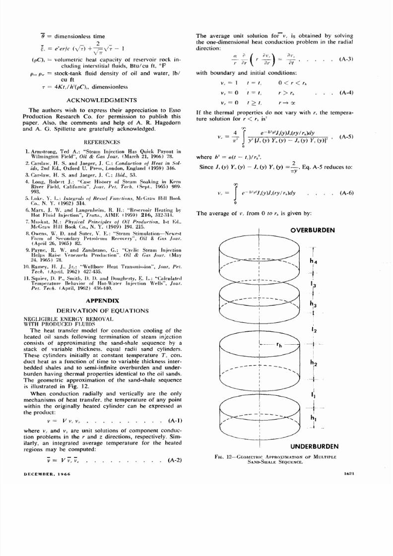
PPENDIX
DERIVATION
OF EQUATIONS
NEGLIGIBLE ENERGY
REMOVAL
WITH PRODUCED FLUIDS
The heat transfer model for conduction cooling
of
the
heated oil sands following termination of steam Injection
consists
of
approximating the sand-shale sequence by a
stack
of
variable thickness. equal radii sand cylinders.
These cylinders initially at constant temperature
T,
COII_
duct
heat as a function
of
time to variable thickness inter
bedded shales and to semi-infinite overburden and under
burden having thermal properties identical to the oil sands.
The
geometric approximation
of
the sand-shale sequence
is
illustrated in Fig. 12.
When conduction radially and vertically are the only
mechanisms of heat transfer. the temperature
of
any point
within the originally heated cylinder can be expressed as
the product:
v = V v,
(A-l)
where v, and are unit solutions of component conduc
tion problems in the rand
z
directions, respectively. Sim
ilarly, an integrated average temperature for the heated
regions may be computed:
v V v
A-2)
DECEMBER 1966
The
average unit solution forv, is obtained by solving
the one-dimensional heat conduction problem in the radial
direction:
~ ~ , - - ( r ~
= ~ ,
r?r (Jr i l l
A-3)
with boundary and initial conditions:
v
=
1
t = t,
0<
r
r
v,
= 0 t
=
t,
r>
r
A-4)
v,. =
0
t
t,
r __
Ct
I f
the thermal properties
do
not vary with
r,
the tempera
ture solution for r < r . is'
if
4 f e-b' fi,(y)J,,(ry/r,,)dy
v, = ' y' [J, (y) Y
n
(y) -
in
(y) Y, (y)]'
(A-5)
o
where b
=
aU
-
t,)/r,, .
Since J
1
(y) Y (y)
- J
(y) Y
1
(y) =2... Eq. A-5 reduces to:
....y
v,,
f)
f e-I>'II J,(y)J,,(ry/r,.)dy
o
The average
of
I',
from 0 to
r
is given by:
,
I
I
I
I
I
OVER URDEN
,
2
t -
UNDER URDEN
FIG.
12-GEOMETRIf . ApPROXIMATION
OF
MULTIPLE
SAND,SHALE
SEQUENCE.
A-6)
1621
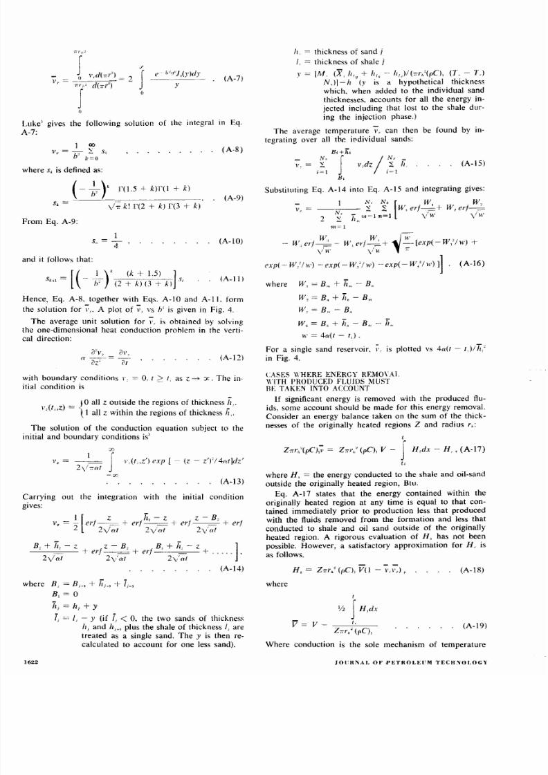
8/10/2019 SPE 1578 PA Boberg Lantz
http://slidepdf.com/reader/full/spe-1578-pa-boberg-lantz 10/11
r
y
e- h'''''},(y)dy
(A-7)
gives
the
following solution
of
the integral
I I I
Eq.
1
00
-
V
r
- -b - Sf.
/ :=0
(A-8)
s, is defined as:
(
l),
- IT
1 (1.5
+ k)T'( 1 + k)
(A-9)
S, =
yr. k
1 (2 +
k)
1 (3 +
k)
Eq. A-9:
1
S, ,=
4
(A-lO)
it follows that:
[
I) (k+1.5)
]
S t l
= -
IT 2 + k) (3 + k) .1',.
(A-II)
Eq. A-8. together with Eqs. A-lO and A-II. form
V,.
A
plot of
v \ s b' is given in Fig. 4.
The average unit solution for
v,
is obtained by solving
heat conduction problem in the verti
direction:
il'v,
ill',
(t ilz' = T t
(A-12l
boundary
conditions
\ ,
=
0,
t
>
t,
as
z
:x.
The
in-
condition is
-
(
)
_
0 all
z
outside the regions
of
thickness h
v. t z - j -
. I all
z within
the regions of thickness II,.
The solution of the conduction equation subject to the
and boundary conditions
is
v =
C/J
I (
2\/-:rl'it
J
-C f
l ',(t z')
exp
[ -
(z
-
z')'/4l'it)dz'
A- l3)
the integration with the initial condition
I [ z .
h,
- z z -
B,
V
Z
= 2
e r l - = +
erf-=+ erl------===-+ erl
2ya t 2y'at 2v'at
B, + ii, - Z + ert z - B, +
-I
B., + ii. - z + ]
_ el
.....•
2\ /at
2v'at
2v al
(A-14)
B, = B,_, + h
j
_,
+ i
j
_,
B
j
= 0
1622
h
j
=
h
j
+
y
i, = - ~ I,
-
y (if i, < 0,
the two sands of
thickness
Iz
j
and h
+, plus
the shale
of thickness I, are
treated
as
a single sand. The y is then re
calculated to account
for
one less sand).
h, = thickness
of
sand j
I
=
thickness
of
shale
j
y = [M. (X, h'q + hI, - hl,V(-:rr,,'(pC), L -
T,)
N J - h (y
is
a hypothetical thickness
which. when
added
to the individual
sand
thicknesses,
accounts
for all the energy in
jected including that lost to
the
shale dur
ing the injection phase.)
The
average
temperature V, can
then be found by in
tegrating over all in.dividual sands:
Bl+hl
N.,
f
, =
;=1 /
N,
_
F,dz
II, .
;=1
(A-l5)
B,
Substituting Eq. A-l4 into Eq. A-15
and
integrating gives:
IN . N. [
W.
: c
W,
er t ,
+ w, erl ,-
T m= l n = l
VW
yw
_ I'I
F , =
2
m = 1
U
l
, W,
~
W·.
-- W, erl .
-
W, ert-;=-+ [exp(
- ,-Iw)
+
yw
V
\I
exp(
- W,'lw)
-exp(
-
W,'lw) -exp - W/lw) ] (A-16)
where U', = B", + iim - B
W, =
B
+ h - Bm
I·V =
B,.,
- B
W; = B + h
-
Bm - ji ,
If
= 4a(
-
t,)
.
For
a single sand reservoir. \ , is plotted vs 4 Y t - l ') lh,'
in Fig. 4.
CASES \\HERE ENERGY REMOYAI.
WITH PRODUCED
FLUIDS
MUST
HE TAKEN INTO ACCOUNT
I f significant energy
is
removed with the produced flu
ids,
some account should
be
made for
this energy removal.
Consider an energy balance taken on the sum of the thick
nesses
of the originally heated regions Z and radius rio:
t
Z r . r , , ( p C ) l ~
= Z-:rr,,' (pC), V
-
f
H,dx - H..,
(A-17)
ti
where H,
= the energy conducted to the shale and oil-sand
outside
the
originally
heated
region, Btu.
Eq. A-17 states
that
the energy contained within the
originally
heated
region
at
any time is
equal to that con
tained immediately
prior to production less
that
produced
with
the
fluids
removed from
the
formation and
less
that
conducted to shale and oil sand outside of the originally
heated region. A rigorous evaluation of
H,
has not been
possible.
However,
a satisfactory
approximation
for
H,
is
as follows.
(A-IS)
where
t
1 12 J ldx
V= V -
t,
Z-:rr,,' (pC) ,
(A-19)
Where conduction
is the sole
mechanism of temperature
JOt:R: I AL OF PETROLEIJM TECH:, \ ,OLOGY
8/10/2019 SPE 1578 PA Boberg Lantz
http://slidepdf.com/reader/full/spe-1578-pa-boberg-lantz 11/11
decay, and the energy removed with the produced fluids is
negligible:
and Eqs. A-I7, A-IS and A-20 reduce to Eq. A-2.17 may
be considered an effective driving force for conduction
which takes into account the effect of temperature reduc
tion due to the removal of energy by the produced fluids.
The definition of 8 from Eq. 5 combined with Eqs. A-
17 through A-19 gives Eq. 4. By Eqs. A-19 and 5:
i = V I -
8
A-20)
Combining Eq. A-20 with Eqs.
A-I7
and
A-IS.
and divid
ing by Z. .r,,'(pCl, gives v
=
V - 2 V8 - V l - 8 I -
v,vol
which simplifies to E4.
4.
Of
several approximations for H, which were tried, the
one used here gave best agreement with field data. Note
that for the limiting case where conduction IS negligible
v,v,
7
1 ,
this approximation gives:
T,,, = T . T, -
T,)[l
- 28]
A-22)
From the definition of 8 this may be seen as giving the
correct value for T
t lvg
in this limiting case.