This work is distributed as a Discussion Paper by the

STANFORD INSTITUTE FOR ECONOMIC POLICY RESEARCH

SIEPR Discussion Paper No. 11-013

ENDOGENEITY IN ATTENDANCE DEMAND MODELS

by Roger G. Noll

Stanford Institute for Economic Policy Research Stanford University Stanford, CA 94305

(650) 725-1874

The Stanford Institute for Economic Policy Research at Stanford University supports research bearing on economic and public policy issues. The SIEPR Discussion Paper Series reports on research and policy

analysis conducted by researchers affiliated with the Institute. Working papers in this series reflect the views of the authors and not necessarily those of the Stanford Institute for Economic Policy Research or Stanford

University.

ENDOGENEITY IN ATTENDANCE DEMAND MODELS

by Roger G. Noll

Abstract

One of the most studied issues in the economics of sports is the nature of the

demand for attendance at sporting events. With few exceptions, the standard result is that

the coefficient on price in the attendance demand equation is either positive or, if

negative, so small that at current prices demand is inelastic. Economists have then

moved on to offering a variety of explanations for why this result may be valid, despite

its inconsistency with theoretical explanations. This paper argues that the cause of price

coefficients that are insufficiently negative is a specification error: the failure properly to

identify the price equation in the supply and demand system. The main conclusion is that

because all teams in a given sport face essentially the same marginal cost of attendance,

the only circumstance in which price can be identified is one in which all or nearly all

games are sellouts and teams play in stadiums of widely varying capacities. Because this

condition is rarely satisfied, the best available econometric procedure is to impose a

restriction on the price coefficient to the effect that the elasticity of demand is one minus

the share of net revenues that are generated by in-stadium sources other than ticket sales

(i.e., parking, concessions, advertising, programs).

Forthcoming, Econometrics in Sports: Proceedings of the Sixth International Conference

on Sports Economics, edited by Stefan Kessenne and Placido Rodriguez Guerrero.

1

ENDOGENEITY IN ATTENDANCE DEMAND MODELS

by Roger G. Noll*

A hoary econometrics principle is that an OLS estimation of a demand equation in which

price is an treated as an exogenous independent variable contains a specification error that is

likely to produce a biased estimate of the coefficient on price.1

Whether the endogeneity of price creates a problem in using OLS to estimate a demand

equation depends on the goal of the regression analysis. If the goal is solely to predict sales as

accurately as possible, endogeneity is not an interesting issue. But if the goal is to estimate the

marginal attendance effect of a particular variable, then endogeneity is a serious problem. For

example, if a goal of a regression is to estimate the price elasticity of demand, a biased estimate

Price is an endogenous variable

that a profit-maximizing supplier chooses on the basis of the cost function and the shape of the

demand relationship. In a single-equation OLS model the coefficient on price measures its

combined effects on demand (negative) and supply (positive). Only if the exogenous shocks to

the equilibrium price and quantity operate to shift the supply curve but not the demand curve will

an OLS estimate of the demand equation produce an unbiased estimate of the coefficient on

price. If the unexplained shocks affect primarily the demand equation, the coefficient on price

will measure primarily the positive response of supply to an increase in price, thereby causing the

estimated equation to trace the supply curve rather than the demand curve.

* Professor Emeritus of Economics, Stanford University, and Senior Fellow, Stanford Institute for Economic Policy Research.

1 For a parsimonious explanation of the endogeneity problem in the public domain, see Daniel McFadden, Lecture Notes, Chapter 6, at http://elsa.berkeley.edu/users/mcfadden/e240b_f01/ e240b.html.

2

of the price coefficient thwarts attaining this goal. Because the price coefficients have opposite

signs in supply and demand equations, endogeneity causes the price coefficient in the demand

equation to be biased upward and the implied price elasticity of demand to be biased downward.

If estimating the price elasticity of demand is not a goal of the regression, an OLS model

still presents a problem. If some variables in the demand equation also appear in the supply

equation, price will be correlated with these independent variables, causing the estimates of these

coefficients to be inefficient. Excluding price from the regression is not a solution because then

the coefficients on the other variables will measure their combined effects on supply and demand

and so be biased estimates of the true demand coefficients.

The endogeneity problem can be addressed by imposing restrictions on the coefficients in

the system of equations. One such identifying restriction is to impose a value on the elasticity of

demand, and hence the price coefficient in the demand equation, that is derived from theory or

other empirical analysis. Identification also can be achieved if some coefficients on exogenous

variables are zero in each equation. A necessary condition for identifying an equation is that

each endogenous explanatory variable is explained in part by an exogenous variable that has a

zero coefficient in the equation to be estimated (the order condition). The order condition is also

sufficient in a two-equation model.2

The endogeneity problem can be corrected by using two-stage least squares in which the

first stage consists of regressing each endogenous variable on all of the exogeneous variables and

the second stage uses the fitted values from the first-stage regressions for the endogenous

2 If an equation has N>1 endogenous right-hand side variables, a sufficient (rank) condition for identifying the equation is that N (or more) exoegenous variables have zero coefficients in the equation to be estimated and that set of coefficients on these variables in the other equations are linearly independent.

3

explanatory variables. Thus, to identify the demand equation, in which quantity is the dependent

variable, actual prices are replaced by fitted values from a reduced form price regression in which

all of the exoegenous variables appear on the right-hand side of the equation. Two-stage least

squares succeeds because it creates a new exogenous variable – the component of an endogenous

variable that is explained by exogenous variables, including the variables that are excluded from

the equation of interest – that is an instrument for the endogenous variable.

In supply and demand models the demand equation frequently is identified by assuming

that the quantity supplied, but not the quantity demanded, is affected by marginal cost, so that

marginal cost (or an instrument for marginal cost, like average cost or input prices) can be used

in the first-stage price regression. The supply equation often is identified by assuming that

demand, but not supply, is affected by demographic characteristics of buyers, which become the

unique exogenous variables in the first-stage quantity equation.3

Sports economists who have estimated attendance demand models

4

3 Another common independent variable in demand equations is income, but income plausibly has a non-zero coefficient in the supply equation because it may be related to the salaries of employees and hence marginal cost. If so, income does not identify either equation.

are aware of the

endogeneity problem, but econometric models of attendance in team sports normally do not take

endogeneity into account. Notwithstanding possible specification error, sports economists

normally include price in the attendance equation. In nearly all of these regressions the price

coefficient is either the wrong sign (positive) or, if negative, sufficiently near zero that it implies

that suppliers set price on the inelastic portion of the demand curve. Sports economists have

generated ex post rationalizations for these results, or as Forrest (2012, p. 178) puts it, “alibis that

4 For surveys of the demand for team sports, see Borland and MacDonald (2003), Cairns, Jennett and Sloane (1985), Fort (2006), and Garcia Villar and Rodriguez Guerrero (2009).

4

might explain that, after all, inelastic demand is consistent with profit maximization.”5 As

Kennedy (2007, p. 397) trenchantly observes: “It is amazing how after the fact economists can

conjure up reasons for incorrect signs” when, in fact, the cause is an econometric problem.6

A few attendance demand models do address the endogeneity problem. In some cases the

analysis simply does not attempt to measaure the effect of price on attendance and instead

estimates reduced form equations to serve some other goal (e.g., Berri, Schmidt and Brook, 2004,

estimate a reduced form revenue equation). Some studies simply include an assumption about

demand elasticity in their list of identifying restrictions (Jones and Ferguson, 1988). A handful

of studies use exogenous instruments for price, including lagged price (Villa, Molina and Fried,

2011), stadium capacity (Garcia and Rodriguez, 2002), or both (Coates and Humphreys, 2007).

This chapter examines the implications of the endogeneity problem in estimating demand

for team sports.7

5 As discussed more fully elsewhere in this chapter, the competing explanations for the finding that demand is price inelastic are: (1) teams do not maximize profits; (2) other revenues, such as concessions and parking, are increased by attendance so that the profitability of the marginal ticket exceeds the ticket price; (3) travel costs to attend games redeuce the elasticity of demand for tickets; and (4) larger stadiums have lower average ticket prices, all else equal, because they have more bad seats, which leads to a downward bias in the estimated effect of lower prices on attendance in a model that does not account for seat quality.

The focus is on the economic theory of the supply of tickets to sporting events

to explore how supply conditions affect price and hence bias the estimated coefficient on price in

6 I am as guilty as anyone of ignoring this problem and offering alibis – see Noll (1974).

7 Other econometric issues that must be taken into account in estimating attendance demand are not discussed here unless they factor in to dealing with the endogeneity problem. One is proper measurement of key variables, such as price (given that teams offer different seat locations at different prices) and competitive balance (for which the relevant variable is the measure of relative team quality that enters the utility functions of fans). Another is the functional form of the demand and supply relationships. Still another is heteroskedasticity, which is likely to arise from population differences and differences in the sample variance of exoegenous variables among localities. A common tool for dealing with this problem is to use the generalized method of moments (GMM) to prodice more efficient estimates of the coefficients (Wooldridge 2001).

5

a reduced form demand model.

This chapter is organized as follows. The first section addresses the issue of finding

appropriate cost variables to identify the demand equation and concludes that this search is futile.

The second section examines the problem of estimating demand for a homogeneous product,

which in the context of attendance at sporting events requires that seats do not differ in quality.

The third section relaxes the homogeneity assumption.

The main conclusions of the analysis to follow are as follows. First, the appropriate

specification of attendance demand depends on whether events are sold out. Second, the demand

equation cannot be identified if games are not sellouts. Third, if events are sellouts, the elasticity

of demand plays no role in determining price and attendance, but the demand equation may be

identified because stadium capacity can explain price and may be exogenous to demand.

Otherwise, the best approach to estimating attendance demand is the one adopted in several

papers in which Colin Jones is a co-author, starting with Jones and Ferguson (1988), which is to

impose a value on the price elasticity of demand, thereby assuming away the empirical finding

that has generated the decades-long debate about its meaning.

USING COST TO IDENTIFY DEMAND

The standard method for identifying the demand equation is to include marginal cost or

instruments for marginal cost in the price (supply) regression. This section explains why this

standard approach is unlikely to be successful in modeling attendance.

The theory of a profit-maximizing, single-product firm predicts that firms will set price so

that marginal revenue equals marginal cost. Assume that the profit function of a team is:

Β = PQ(P) – mQ,

6

in which P is price, Q is attendance and m is the marginal cost of selling a ticket and

accommodating a fan. The first-order condition for profit maximization is the following:

(1) P = m – Q/Q/.

Expression (1) forms the basis for the standard supply equation in a two-stage least-squares

model. Price is regressed on marginal cost (or instruments for marginal cost, such as input

prices) and the other exogenous variables, and the estimates of price from this equation are used

as an instrument for price in the demand equation. The coefficient on price is then an unbiased

estimate of the true coefficient if the model contains no other specification error.

Expression (1) yields insights about the elasticity of demand at the equilibrium price that

have informed the debate about the findings that the demand for attendance at sports events in

price inelastic. Rearranging expression (1) yields the following:

(2) m = P(1+e)/e,

in which e<0 and |e| is the price elasticity of demand. If m=0, expression (2) implies that e=-1,

i.e. that price is set at the unit elasticity point on the demand curve. If m>0, the Lerner Index,

which is the equilibrium markup of price over marginal cost, is the following:

(3) (P–m)/P = -1/e.

Because profit maximization requires P–m>0, expression (3) implies e<-1 and so |e|>1, i.e., that

the firm sets price on the elastic portion of demand. If empirical models find that |e|<1, at least

one of the following statements must be true:8

8 A fourth explanation for inelastic demand is that ticket prices do not equal the full cost of attendance, which also includes travel costs (Noll, 1974; see Forrest, 2012, for a survey of studies of the effect of travel cost on sports demand). If attendance demand is a function of total costs of attendance, then a change of z percent in ticket price will lead to less than a z percent change in total costs, which means that at any given ticket price the demand for tickets is less elastic than it would be if travel costs were zero. Thus, teams face a demand curve that is less

(1) specification error has caused the estimate of

7

the coefficient on price in the demand equation to be biased upwards and the conclusion that

demand is inelastic is erroneous; (2) the profit equation that sports enterprises maximize is not

accurately represented as the revenues and costs associated with attendance; or (3) sports

enterprises do not maximize profits.

Accounting for Specification Error

The first explanation for a coefficient on price that is too high is that including price in

the attendance equation is a serious specification error. As discussed above, the conclusion to be

drawn from the theory of the firm is that marginal cost can be used as an instrument for price that

can identify the demand equation.

In sports the short-term marginal cost of attendance is the cost of selling one more ticket

and allowing an additional fan to attend the game. As first observed by Demmert (1973), the

short-run marginal cost of attendance is very low and does not exhibit much variation among

suppliers of events in the same sport. The implication of a marginal cost near zero is that in

equilibrium the price elasticity of demand will be near one. For example, if the marginal cost of

selling tickets and accommodating fans is five percent of the ticket price, the implied equilibrium

price elasticity of demand is approximately1.05. For dealing with the endogeneity of price in the

attendance equation, the more important issue is the lack of variability in short-run marginal cost

among sports enterprises. Short-run marginal cost cannot identify the price equation if marginal

cost is essentially a constant across teams or, for the same team, over time.

elastic at each price. Assuming a marginal cost of attendance, the profit-maximizing ticket price still occurs at the unit elasticity point of the residual demand for tickets, but the equilibrium price will be higher (and attendance lower) than would be the case if travel costs were zero. Hence, travel costs do not explain inelastic demand at the equilibrium price.

8

In analyzing the appropriate specification of a supply and demand model in team sports,

Fort (2004) argues that team quality affects the marginal cost of attendance because a team can

attract more fans by spending more on talented players and coaches. If all teams compete in the

same markets for talented inputs, the price of talent will be the same for all teams; however, the

marginal quality cost of attendance can differ among teams. In equilibrium, the marginal

revenue of team quality equals its marginal cost. A variant of Fort’s team profit function is:

Β = PQ(P,x) – mQ(P,x) – wx,

where x is quality, w is the unit wage of skills, and P, Q and m are defined as in expression (1),

the first-order condition for quality is as follows:

(4) w/(δQ/δx) = (P–m).

The left side of equation (4) is the cost of attracting one more fan by improving quality. Because

teams do not all set the same price, the left side of expression (4) must vary among teams. If

talent markets are competitive, teams face the same price of talent, w, so the source of variation

in expression (4) must be δQ/δx, which implies that the relationship between team quality and

attendance is not linear. If attendance exhibits diminishing returns to talent, which is consistent

with the proposition that fans value competitive balance, the marginal attendance effect of team

quality is decreasing in talent. From expression (4), diminishing returns to talent implies that

high values of δQ/δx are associated with low values of attendance, price and team quality.

For purposes of identifying the demand equation, the relevant question is whether the

marginal attendance productivity of talent, δQ/δx, or perhaps an instrument for it, is a valid

exoegenous variable in the price equation but not the attendance equation. The arguments of

δQ/δx are price, team quality and the exogenous variables in the attendance equation. Hence, the

marginal quality cost of attendance is endogenous in the price equation and so cannot be used as

9

an exogenous instrument for price. Moreover, any exoegenous variable that affects the marginal

productivity of talent appears in both the demand and supply equations and so does not satisfy

the order condition for identification.

The sad news from the preceding analysis is that one cannot adopt a normal identification

strategy of using cost as an instrument for price. Neither marginal cost nor any instrument for

marginal cost can be regarded as a unique exogenous variable in the first-stage price regression.

The Opportunity Cost of Lower Attendance

The second explanation for a coefficient on price that is not sufficiently negative is that

the firm’s profit maximization problem is not accurately characterized in the preceding analysis

(Heilmann and and Wendling, 1976, Coates and Humphreys, 2007, and Krautman and Berri,

2007). Net revenue from attendance exceeds ticket sales because teams also profit from non-

ticket game-day revenue sources, such as concessions, in-stadium advertising, and, in many

cases, parking, all of which are related to the number of fans who attend the event. These other

revenues create an opportunity cost for a decision to exclude more fans by raising ticket prices, in

which case this opportunity cost is a candidate for explaining price and identifying demand.

A variant of the profit function from Heilmann and Wendling (1976) is the following:

Β = PQ(P) + R(Q(P)) – mQ,

where R(Q(P)) is the net revenue accruing to the team from sources other than ticket sales that

depend on attendance. The first-order condition for this profit function then is the following:

(5) P = m – Q/Q/ – R/,

which can be rearranged to become:

(6) (P-m)/P = 1/|e| – R//P.

10

Thus, the profit-maximizing Lerner Index is less than the inverse of the elasticity of demand,

with the difference being the ratio of the marginal revenue from other sources to the price of a

ticket. If the marginal cost of attendance (m) is zero, expression (6) implies the following:

(7) |e| = P/(P + R/).

The relative importance of non-ticket revenues and ticket sales in the profit equation

differs among sports, so expression (7) implies that the equilibrium price elasticity of demand

also should vary among sports. For example, if non-ticket game-day revenues are a small

fraction of ticket prices (e.g., the National Basketball Association in the U.S.), |e| should be close

to unity. If non-ticket revenues are at least as important as ticket sales (e.g., the lowest

classifications of American minor league baseball), the value of |e| should not exceed 0.5. Thus,

the plausibility of this explanation for finding that demand is inelastic depends on the sport, but

could explain an elasticity of demand substantially less than unity for a sport in which non-ticket

game-day profits are comparable in importance to revenues from ticket sales.

Expression (5) also has implications for identification. If teams exhibit little or no

variation in m, they still might exhibit variation in marginal non-ticket revenues, R/. If so,

expression (5) suggests that a measure of the marginal profitability of non-ticket game-day

revenues might be used as an instrument for price. A possible measure of the marginal

profitability of non-ticket revenue sources is average non-ticket revenue, which works as an

instrument if the profitability of these products exhibits constant returns to scale in attendance.

Unfortunately, non-ticket game-day revenue is not likely to be a valid identifier. Revenue

from these sources is endogenous because teams decide the variety and prices of these products.

Nevertheless, teams often sign long-term contracts with other firms to provide these products, in

which case these revenues are exogenous in the short run. But even if this variable is

11

exoegenous, attendance plausibly could be affected by the variety and prices of these products

(Coates and Humphreys, 2007). If so, non-ticket average revenue cannot be used as an

instrument for price to identify demand because it appears in both equations.

The Dubious Test for Profit Maxmization

As the orginal perpetrator of using estimates of the price elasticity of demand as a “test”

for profit maximization, I confess that this test is not valid. The reason that this test is erroneous

sheds interesting light on specification of attendance demand.

Consider a simple alternative to profit maximization, which is that teams maximize on-

field victories subject to a budget constraint. If so a firm has the following objective function:

W = F(x)

where W is wins and F is a function that maps team quality, x, into victories. The maximization

of wins is subject to the budget constraint:

K + PQ(P,x) > mQ(P,x) + wx,

where K is the owner’s cash contribution to operations and all other terms have the same

definitions as in the preceding analysis. The owner’s optimization problem is to maximize:

(7) W = F(x) – λ(K + PQ(P,x) – mQ(P,x) – wx).

where λ is the Lagrange multiplier. Except for K, the term inside the Lagrange multiplier in

expression (7) is the profit function when team quality is a choice variable for the firm. Because

K is a constant and x does not depend on price, the first-order condition for maximizing

expression (7) is identical to the first-order condition for price in the simple profit-maximization

model, which is expression (1). Hence, the equilibrium price elasticity of demand in the win-

maximization model is that same as in the profit-maximization model. Thus, the finding that

12

demand is inelastic rejects the win-maximization model.

The price-elasticity test also is doubtful as a test of the validity of a model of a sports

enterprise as maximizing the utility of the owners. As originally proposed by Sloane (1971, p.

136) owner utility is a function of attendance, team quality, profits, and league viability. The

last depends on the quality of the team and the subsidy a team gives to other members, which in

turn is depends on team quality. Hence league viability is taken into account in the functional

relationship between team quality and utility. The implied objective function is then:

(8) U( π, x, Q) = U(PQ(P.x) – mQ(P,x) – wx, x, Q(P,x)).

If profits and wins were the only arguments in the utility function, the equilibrium price

elasticity would not differ among utility maximization, win maximization and profit

maximization models. In finding the maximum of expression (8), the first-order condition for

price is that the marginal utility of profit multiplied by the marginal profit of a price change

equals zero. Because the marginal utility of profit always is positive, the marginal profit of a

price change must be zero, which is the same first-order condition for price as in the other

models. But if attendance is a separate argument of the utility function, the first-order condition

for price contains another additive term: the product of the marginal utility of attendance and the

marginal effect of price on attendance effect. The new equation that is the counterpart to

expression (1) is then as follows:

(9) P = m – Q/Q/ – UQ/Uπ,

where UQ/Uπ is the marginal utility of attendance divided by the marginal utility of profit.

Because the marginal utilities of attendance and profit are both positive, expression (9) implies

that the equilibrium price elasticity of demand is lower than in the other models. If m=0, the

price elasticity of demand is given by:

13

|e| = 1/(1 + UQ/Uπ) < 1.

The equilibrium price elasticity that is derived from Sloane’s model is similar to the result

from the model that includes attendance-related revenues other than ticket sales. Thus, whether

the demand for tickets is inelastic is actually a test of whether attendance contributes value

beyond revenues from ticket sales, regardless of whether this added value comes from profit or

owner utility. Because attendance can add value to either utility or profit from other sources, the

presence of inelastic demand for tickets is a test of whether attendance creates value beyond

ticket sales and not of the motivation of owners.

SUPPLY OF HOMEGENEOUS SEATS

An important complication in estimating the demand for sports is that the product being

supplied – a seat at a sporting event – is not a homogenous product. That is, a fan’s enjoyment of

the event depends on seat location, which causes suppliers to price tickets on the basis of seat

quality. The analysis in this section ignores heterogeneity in seats for the purpose of developing

a baseline model of supply and demand that transparently illustrates the endogeneity problem and

the implications of sellouts. The next section relaxes this assumption.

The point of this section is illustrated in Figures 1 and 2. In these figures the vertical axis

is a value measure (here euros) and the horizontal axis is a quantity measure (here attendance).

Figure 1 depicts supply and demand conditions for two teams, one of which faces high

demand, DH, and the other faces low demand, DL. These demand relationships can be interpreted

as pertaining to teams in large and small markets, respectively. Figure 1 also shows the stadium

capacity for both teams, S, which exceeds the equilibrium demand for both teams. Price and

quantity are written as Pi and Qi, respectively, with i indexing demand (i = L, H). The

14

equilibrium price and quantity is determined by the point at which marginal revenue equals

marginal cost. As is standard in the literature on attendance demand, marginal cost is assumed to

be zero. Equilibrium prices are PL and PH and equilibrium values for attendance QL and QH.

Figure 1 shows that when stadium capacity exceeds equilibrium attendance for all teams

and all teams have the same marginal cost, price and quantity both will be increasing as the

demand curve shifts outward. In Figure 1, PL < PH and QL < QH. Thus, if attendance is regressed

on price, the coefficient will be positive. In principle the exogenous independent variables that

affect attendance can account perfectly for the difference between DL and DH. That is, if the

differences between the two teams in all non-price variables were fully taken into account, the

underlying demand relationships for both teams would be identical. Because both teams have the

same marginal cost of attendance (here zero), the equilibrium price and attendance for the two

teams would be identical if the values of the exogenous variables were the same for both teams.

Thus, there is no variance in price to be explained by other exogenous variables, and the demand

equation cannot be identified.

In practice the specification of the relationsahip between demand and the exoegenous

variables is unlikely to be perfect. Some exogenous variables that affect demand may be missing

from the equation (for example, a measure of variation in the interest in the sport among

communities). For some exogenous variables their instruments may be imperfect (for example,

population density is an imperfect instrument for ease of access to the playing site). The

estimated coefficient on price then will soak up the unexplained variance in the equation that

arises from these specification errors. As a result, the estimated coefficient on price is biased.

Indeed, the coefficient on price reflects only the specification error if there is no independent

source of variation in price that can be used as an identifier in the price regression.

15

Figure 2 depicts a circumstance in which all teams face the same demand curve, but

teams have stadiums with different capacities, SL, SM and SH for low, medium and high capacity,

respectively. These capacities produce equilibrium prices of PL > PM > PH, and the locus of

equilibria for varying capacities tracees the demand curve. Thus, the demand equation can be

identified by including capaxcity in the first-stage price equation. The trick here is that each

vertical segment of a team supply curve is associated with a shadow price of stadium capacity

that serves as an implicit marginal cost of attendance that varies across teams.

Suppose that the demand curve in Figure 2 is actually the average demand curve that

arises if all of the exogeneous variables that affect attendance take their mean values. One can

imagine a family of demand curves that apply to teams in different markets. The true team

demand curves are a series of downward sloping lines in an amended Figure 2 (as in Figure 1),

and the resulting price/quantity equilibria resemble a shotgun blast. But the exogenous demand

variables account for the shifts in demand among teams and capacity then determines price, so a

valid two-stage least squares estimate is possible.

A potential problem with using capacity to identify the demand equation is that capacity

may an endogenous variable that is selected on the basis of demand. Surely when sports

facilities are constructed, the underlying popularity of the sports that will use the facility enters

into the decision about capacity. The potential salvation for capacity as an exogeneous identifier

is that sports facilities have a long useful life, implying that capacity is exogenous for nearly all

teams in nearly all years. But stadium capacity still is likely to bear some relationship to

attendance because the variables that determine the popularity of a sport are likely to be

correlated through time.

The crucial issue for identification is whether shocks to demand after a facility is built are

16

correlated with capacity. Capacity can be used to trace changes in price along the demand curve,

and hence in the first-stage price equation, only if capacity is uncorrelated with shifts in demand

through time.

A test for whether capacity can identify the demand is to regress capacity on the current

values of the exogenous variables that appear in the demand equation. If the fit is good, then

capacity is a weak identifier and cannot be expected to allow an unbiased estimate of the

coefficient on price in the attendance equation (Wooldridge, 2001). A poor fit implies that

capacity is mainly exogenous to demand, but it still can be a weak identifier. For example, in

leagues such as the NFL in which capacity does not exhibit much variation among teams, the fact

that capacity passess a test for endogeneity is likely to be small comfort because its variance is to

small to provide much explanatory power for price.9

A similar set of observations applies to the common use of lagged price as an exogenous

instrument for current price. The relevant statistical concept for identification is not whether the

current values of the other exogenous values possibly could cause historical prices, but whether

mathematically historical prices can be approximated by a linear combination of the current

values of these variables. If the fit of a regression of lagged prices on current values of

exoegenous variables is good, lagged prices are a weak identifier. If the fit is poor but a

substantial amount of the variation in current prices is explained by lagged prices, the latter may

bbe a valid instrument for the former, but such a result raises the question about why this

9 Coates and Humphreys (2007) find that in analyzing NFL attendance, using capacity in the first-stage price regression yields coefficients on both price and the total cost of attending a game that have the wrong sign. Two possible explanations for this result are that capacity is a weak identifier or that variation in capacity among teams actually is an instrument for an omitted variable or other specification error in the demand equation.

17

correlation exists. Because in any period price is not really exogenous, the cause on

intertemporal correlation of price is almost certainly due to an omitted exoegnsous variable that

enters either the cost function or the demand function. In this case, lagged price actually is an

instrument for this variable. Without further information about the identity of the omitted

variable and the mechanism through which it affects price, one cannot tell whether incorporating

it into the price equation identifies the demand equation.

SUPPLY FROM A MULTI-PRODUCT FIRM

The previous analysis departs from reality because sports facilities have seats of varying

quality. A ticket to a sports events is not a homogeneous product, but tickets for seats of

differing quality are separate products that are imperfect substitutes. This section explores the

decision by ba profit-maximizing sports team about how to price seats of varying quality, given

that lower prices for lower quality seats can ‘cannabilize” sales of better seats at higher prices.

To simplify for clarity, assume that a team has a fixed supply of good seats, SG, and bad

seats, SB. This section ignores the issues of the endogeneity of team quality and the presence of

attendance-related revenue other than ticket sales. The results that arise from generalizing the

model parallel the results for the case of homogeneous seats. Hence, here we assume that the

team maximizes profits subject to the constraints that sales of both types of tickets cannot exceed

the respective capacities:

(10) π = PGQG(PG,PB) + PBQB(PB,PG) – m(QG–QB) – λG(QG – SG) – λB(QB – SB),

where the variables are as defined above except that the subscripts, G and B, refer to good and

bad seats. The assumption that the marginal cost of attendance is equal for good and bad seats

simplifies the results and is no great sacrifice of reality if the marginal costs of both types of

18

attendance are near zero.

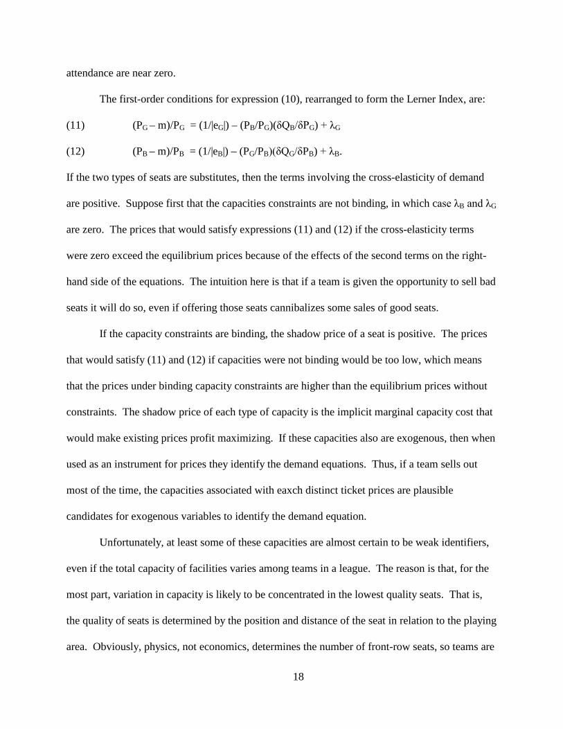
The first-order conditions for expression (10), rearranged to form the Lerner Index, are:

(11) (PG – m)/PG = (1/|eG|) – (PB/PG)(δQB/δPG) + λG

(12) (PB – m)/PB = (1/|eB|) – (PG/PB)(δQG/δPB) + λB.

If the two types of seats are substitutes, then the terms involving the cross-elasticity of demand

are positive. Suppose first that the capacities constraints are not binding, in which case λB and λG

are zero. The prices that would satisfy expressions (11) and (12) if the cross-elasticity terms

were zero exceed the equilibrium prices because of the effects of the second terms on the right-

hand side of the equations. The intuition here is that if a team is given the opportunity to sell bad

seats it will do so, even if offering those seats cannibalizes some sales of good seats.

If the capacity constraints are binding, the shadow price of a seat is positive. The prices

that would satisfy (11) and (12) if capacities were not binding would be too low, which means

that the prices under binding capacity constraints are higher than the equilibrium prices without

constraints. The shadow price of each type of capacity is the implicit marginal capacity cost that

would make existing prices profit maximizing. If these capacities also are exogenous, then when

used as an instrument for prices they identify the demand equations. Thus, if a team sells out

most of the time, the capacities associated with eaxch distinct ticket prices are plausible

candidates for exogenous variables to identify the demand equation.

Unfortunately, at least some of these capacities are almost certain to be weak identifiers,

even if the total capacity of facilities varies among teams in a league. The reason is that, for the

most part, variation in capacity is likely to be concentrated in the lowest quality seats. That is,

the quality of seats is determined by the position and distance of the seat in relation to the playing

area. Obviously, physics, not economics, determines the number of front-row seats, so teams are

19

not likely to exhibit much variability in the number of top quality seats that they offer. As a

result, regressing price on capacity is not likely to produce a useful instrument that identifies the

demand equation for better seats.

Frequently attendance demand studies deal with the heterogeneity of seats by constructing

an average price over all types of seats. In the above model, an illustration would by to construct

the average price, PA = (PGSG + PBSB)/(SG + SB). In some cases, total capacity is then used as an

exoegenous variable to explain average price in a first-stage regression, the fitted values from

which are then used as the instrument for price in the second-stage regression. This procedure

cannot possibly identify demand if capacity is not binding because capacity is not an instrument

for any price variable.

If capacity is binding, the effects of using capacity as an instrument for price require

taking into account the true structure of the supply and demand relationship for the team as a

multi-product firm (two types of seats). That is, the true structural model has two separate

demand and supply equations. The estimated supply and demand equations are then sums of the

two true equations. The actual sum of the true demand equations is:

(13) QG + QB = a + bGPG + bBPB + cZ,

where scalers a, bG and bB and vector c are parameters to be estimated and Z is a vector of

exogenous variables. One can imagine two approaches to using capacity to identify the prices in

this regression.

One approach is to undertake separate first-stage regressions on the two prices, with the

capacities for the two types of seats exogenous variables that do not appear in the demand

equation. Two problems arise from using this approach. The first is that the estimated

coefficients on prices in expression (13) combine two effects: the effect of a price for a given

20

seat quality on demand for that quality of seat (a measure of own elasticity) and the effect of the

price for one quality of seat on demand for the other quality (a measure of cross-elasticity). The

second is that for good seats the identifier is weak because of lack of variation across teams, in

which case the equation is not really identified.

The other approach is to use average price as a single price variable and to estimate a

first-stage regression of price on total capacity and the other exogenous variables. The actual

estimating equation is then:

(14) QG + QB = a + b(PGSG + PBSB)/(SG + SB) + cZ

This procdure amounts to imposing another restriction on the price coefficients, bG and bB, that

they each are equal to b multiplied by the share of seats at the associated quality. The resulting

estimated value is b is even less meaningful than the estimates of separate coefficients in

expression (13). The restrictions have no basis in economics, and hence yield poor estimates of

the underlying coefficients in (13). Moreover, by imposing this restriction, the presence of a

weak instrument for PG is allowed to infect the estimated hybrid coefficient on PB.

The take-home message of this analysis is that the use of average ticket prices, even when

the averages are based on capacities instead of sales, is not a valid procedure. The best that one

can do is to match each ticket price to the number of seats at that capacity and then, for the subset

of prices for which its seat capacity is not a weak instrument, include only fitted values of those

prices in the demand equation.

CONCLUSIONS

The preceding analysis supports fairly gloomy conclusions. The first conclusion is that

identifying an attendance demand equation by finding a good instrument for price is not likely to

21

succeed. Second, the only plausible instrument is capacity, and this is likely to work only for bad

seats when teams have mostly sellouts and when capacity exhibits substantial variation among

teams in a league. Third, demand models ought to include separate equations for each quality of

seat, and every equation should contain instruments for each price, derived from first-stage

regressions of price on all exoegenous variables, including all the capacities for each seat quality.

Most likely, such an estimation is impossible, in which case the best strategy is to assume that

theory is accurate and to restrict the value of the price coefficients that cannot be reliably

estimated. These coefficients should be based on the assumption that the own price elasticity of

demand is near one, adjusted downward for the proportion of net revenues from attendance-

related sources other than ticket sales.

22

REFERENCES

Berri, David J., Martin B. Schmidt and Stacey L. Brook (2004). “Stars at the Gate: The

Impact of Star Power on NBA Gate Revenues.” Journal of Sports Economics Vol. 5, No. 1

(February), pp. 33-50.

Borland, Jeffrey, and Robert MacDonald (2003). “Demand for Sport.” Oxford Journal

of Economic Policy Vol. 19, No. 4 (December), pp. 478-502.

Cairns, John A., Nicholas Jennett and Peter J. Sloane (1985). “The Economics of

Professional Team Sports: A Survey of Theory and Evidence.” Journal of Economic Studies

Vol. 13, No. 1, pp. 3-80.

Coates, Dennis, and Brad R. Humphreys (2007). “Ticket Prices, Concessions and

Attendance at Professional Sporting Events.” International Journal of Sport Finance Vol. 2, No.

3, pp. 161-170.

Demmert, Henry (1973). The Economics of Professional Sports. Lexington,

Massachusetts: Lexington Books.

Forrest, David (2012). “Travel and Population Issues in Modelling Attendance Demand.”

In Stephen Schmanske and Leo H. Kahane (eds.), The Oxford Handbook of Sports Economics

Vol. 2. New York: Oxford University Press, pp. 175-189.

Fort, Rodney (2004). “Inelastic Sports Pricing.” Managerial and Decision Economics

Vol. 25, No. 2 (March), pp. 87-94.

_________ (2006). “Inelastic Sports Pricing at the Gate? A Survey.” In Wladimir

Andreff and Stefan Szymanski (editors), Handbook on the Economics of Sport. Cheltenham,

United Kingdom: Edward Elgar Publishing.

Garcia, Jaume, and Placido Rodriguez (2002). “The Determinants of Football Match

23

Attendance.” Journal of Sports Economics Vol.3, No. 1 (February), pp. 18-38.

Garcia Villar, Jaume, and Placido Rodriguez Guerrero (2009). “Sports Attendance: A

Survey of the Literature 1973-2007.” Revista di Diritto Ed Economia dello Sport, Vol. 5, No. 2,

pp. 111-151.

Heilmann, Ronald L., and Wayne R. Wendling (1976). “A Note on Optimum Pricing

Strategies for Sports Events.” In Robert Engel Machol and Shaul P. Ladany (eds.), Management

Science in Sports. New York: North Holland Publishing, pp. 91-100.

Kennedy, Peter (2007). A Guide to Econometrics. Malden, Massachusetts: Blackwell

Publishing.

Krautman, Anthony C., and David J. Berri (2007). “Can We Find It in the Concessions?

Understanding Price Elasticity in Professional Sports.” Journal of Sports Economics Vol. 8, No.

2 (April), pp. 183-91.

Noll, Roger G. (1974). “Attendance and Price Setting.” In Roger G. Noll, editor,

Government and the Sports Business. Washington D.C.: Brookings Institution, pp. 115-58.

Schmidt, Martin B. (2012). “Demand, Attendance and Censoring: Utilization Rates in

the National Foootball League.” In Stephen Shmanske and Leo H. Kahane (editors), Oxford

Handbook of Sports Economics, Vol. 2. New York: Oxford University Press, pp. 190-200,

Sloane, Peter J. (1971). “The Economics of Professional Football: The Football Club as

a Utility Maximizer,” Scottish Journal of Political Economy Vol. 18, No. 2 (June), pp. 121-146.

Wooldridge, Jeffrey M. (2001). “Applications of Generalized Method of Moments

Estimation,” Journal of Economic Perspectives Vol. 15, No. 4 (Fall), pp. 87-100.

Figure 1: Price and Attendance with High Stadium Capacity

€

PH

-------------------------------- | PL

------------------------ | | | | | | | | | | | DL

| | DH

|MR* | MR QL QH S Q (Attendance)

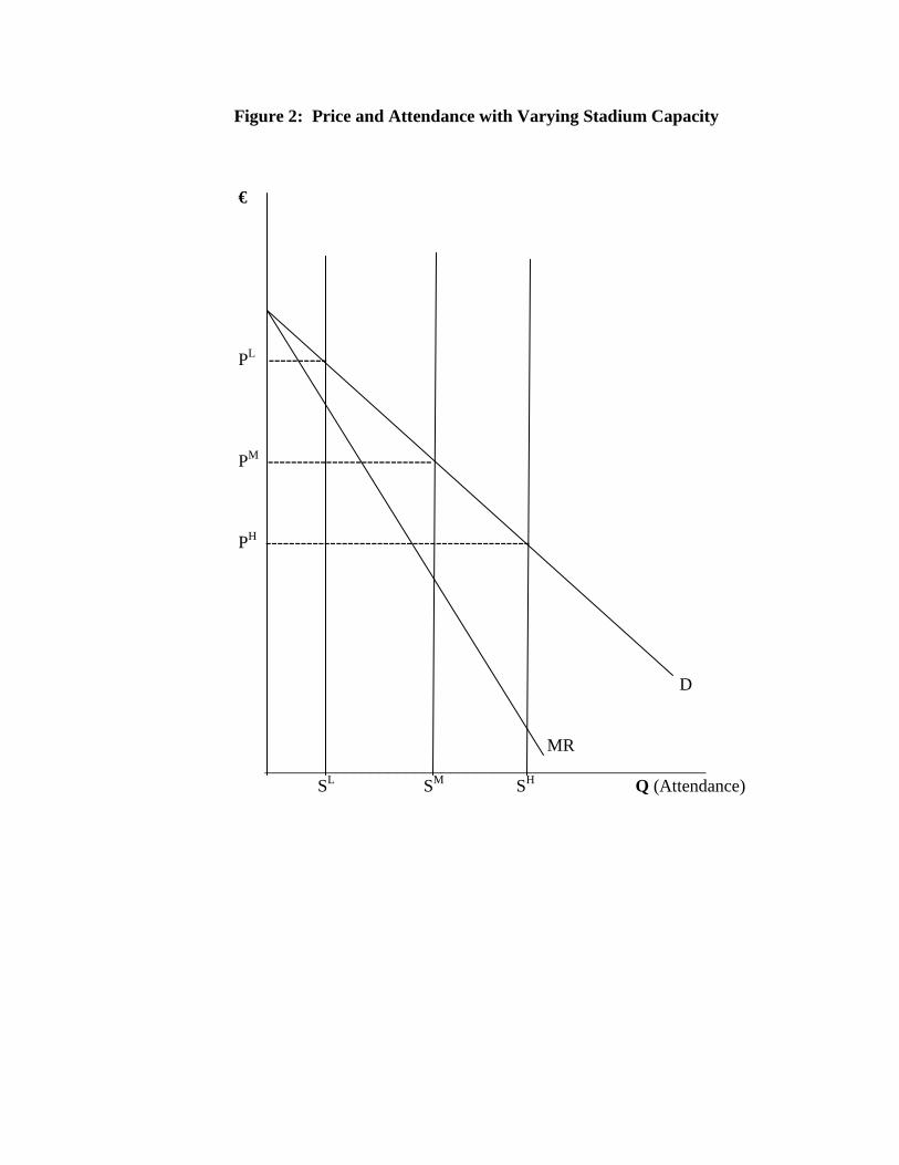
Figure 2: Price and Attendance with Varying Stadium Capacity

€

PL ----------

PM ----------------------------

PH ---------------------------------------------

D MR __________________________________________________ SL SM SH Q (Attendance)