Spoilt for Choice? An Investigation Into Creating Gastner andNewman-style Cartograms

Chris Brunsdon ∗1 and Martin Charlton †1

1Maynooth University National Centre for Geocomputation

January 8, 2015

Summary

A number of choices are encountered when creating cartograms using the Gastner and Newmanalgorithm. Two important ones are the starting map projection, and the resolution of the grid size used to

compute the cartogram transform. We experiment with a number of projection and grid sizecombinations, and define a measure of ‘cartogram success’, and use this, together with a moredescriptive assessment, to identify best practice in choosing resolution and initial projection.

KEYWORDS: Cartogram, Rasterisation, Visualisation, Cartography, Map Projection

1 Introduction

Cartograms are well established map projections used for the creation of statistical maps that take into ac-count the underlying population of geographical reporting units (GRUs). They have the property that theprojected area of each areal unit is proportional to its population1. There are a number of standard algo-rithms to compute cartograms - see for example Tobler (1973), Dorling (1996) or Sagar (2013). Most ofthese begin with a standard map projection, with populations supplied for each GRU, and then compute a’warp’ - of the map drawn in this projection to obtain the cartogram. One particular example of this approachis the Gastner and Newman algorithm (Gastner and Newman, 2004). This solves the diffusion equation -Equation 1 below, using a pixel-based approximation.

∂ρ(x, y, t)

∂t= ∇2ρ(x, y, t) (1)

This equation describes the flow of fluids with varying density ρ at time t and at each location (x, y). Forcartograms, it is assumed that ρ is proportional to population density. Study of Equation 1 reveals that fluids∗christopher.brunsdon@nuim.ie†martin.charlton@nuim.ie1At least approximately

will diffuse towards an asymptotic state of uniform density. Thus, for each initial location the mapping ontoa particle’s asymptotic location provides a cartogram transformation.

1.1 Spoilt for choice?

A number of observations can be made about this algorithm.

1. The method is based on approximation.

2. It depends on a grid-based estimation of population density.

3. This estimation is derived from a map using a conventional projection. Several such projections exist.

These raise a number of issues - observation 2 suggests that a number of choices must be made prior torunning the cartogram algorithm - namely, at what resoluton should the grid be created, and what methodshould be used to estimate the density values in the grid. Observation 3 implies a further choice - that ofthe starting map projection - and observation 1 leads to an over-arching issue that, although the cartogramalgorithm is often presented as a unique process, there are in fact a number of degrees of freedom. Theaim of this paper is to investigate the effect of varying these, and hopefully uncover some ‘best practice’recommendations for the creation of cartograms.

2 Choices for Initial Conditions

The two key choices relate to the initial map projection, and the resolution of the grid used in the numericalsolution of the diffusion equation. The Gastner and Newman algorithm begins with a set of initial densities- typically these are obtained from a set of polygons in a ‘conventional’ map projection with associatedpopulation counts, and assigning population density estimates to each polygon by dividing the count by thecorresponding polygon areas. The results are then converted to a raster grid before applying the algorithm- each pixel is assigned to a polygon (approximately) and the density associated with that polygon is thenassigned to the pixel – at which point the algorithm is applied.

2.1 Choice of Initial Map Projection

There are several ‘conventional’ map projections2, and several possible starting configurations for the algo-rithm. Map projections can be classified in a number of ways, but one helpful approach here is to use thefollowing classes:

• Equal Area - These are projections that give polygons whose area is the same as that on the surfaceof the Earth. One cost of achieving this is that shapes of areas are prone to distortion.

• Conformal - These projections preserve local angles, so that the projected angles where curves meetagree with those on the Earth’s surface.

2actually an infinite number if parameters such as the location of parallels are allowed to vary

• Equidistant - These preserve distances from some fixed point, or line on the Earth’s surface.

• Compromise - These do not attempt to preserve area, distance or local angles, but instead aim to strikea balance between the distortions, in order to produce æsthetically pleasing results.

Projections may also be classified by the developable surface onto which the Earth’s surface is projected:cones, cylinders and planes are typical examples (Bugayevskiy and Snyder, 1995). This leads to a crossclassification of surface and property, which often features in the name: for example, Lambert’s AzimuthalEqual Area is an area preserving projection based on a plane.

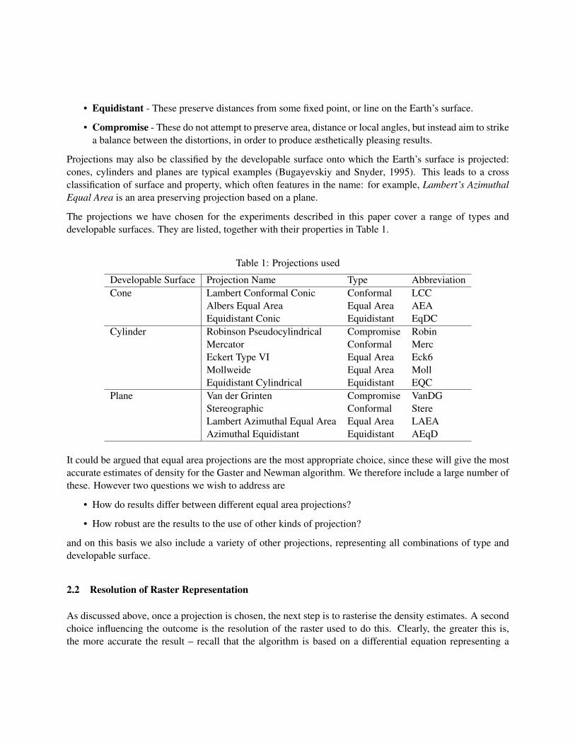
The projections we have chosen for the experiments described in this paper cover a range of types anddevelopable surfaces. They are listed, together with their properties in Table 1.

Table 1: Projections used

Developable Surface Projection Name Type AbbreviationCone Lambert Conformal Conic Conformal LCC

Albers Equal Area Equal Area AEAEquidistant Conic Equidistant EqDC

Cylinder Robinson Pseudocylindrical Compromise RobinMercator Conformal MercEckert Type VI Equal Area Eck6Mollweide Equal Area MollEquidistant Cylindrical Equidistant EQC

Plane Van der Grinten Compromise VanDGStereographic Conformal StereLambert Azimuthal Equal Area Equal Area LAEAAzimuthal Equidistant Equidistant AEqD

It could be argued that equal area projections are the most appropriate choice, since these will give the mostaccurate estimates of density for the Gaster and Newman algorithm. We therefore include a large number ofthese. However two questions we wish to address are

• How do results differ between different equal area projections?

• How robust are the results to the use of other kinds of projection?

and on this basis we also include a variety of other projections, representing all combinations of type anddevelopable surface.

2.2 Resolution of Raster Representation

As discussed above, once a projection is chosen, the next step is to rasterise the density estimates. A secondchoice influencing the outcome is the resolution of the raster used to do this. Clearly, the greater this is,the more accurate the result – recall that the algorithm is based on a differential equation representing a

continuous system. On the other hand, computation time will increase with resolution - and it will be usefulto identify a point at which no notable improvements are achieved, so that unneccesarily long program runsare avoided. Thus, for each map projection, cartograms are created at a number of resolutions. In each casethe raster is square, and of size n× n where n is one of {512, 768, 1024, 1280, 1536}.

3 Evaluation

The set of map projections and resolutions outlined above were used to compute cartograms of Europeaneconomic regions. The software used was Brunsdon’s getcartr package in R3. Cartograms are assessed in twoways here. Firstly, an objective scoring system is used. Although based on approximation, the transformedareas in a cartogram should ideally be proportional to their underlying populations. Thus, if a cartogramalgorithm has worked effectively, then

Ai = kPi (2)

where Ai is the area of a zone i (in cartogram space), Pi is the corresponding population, and k is someconstant value. Thus, for any given cartogram, fitting a least squares regression line without an interceptshould give an estimate of k, say k. Perhaps more usefully, looking at the size of the residuals - that isthe values of Ai − kPi gives an indication of how well this linear fit has worked for each area. Squaringthese residuals and summing gives an overall measure of the degree of disagreement in the proportionalitybetween area and population and hence a measure of the success of the cartogram. As a further enhancement,the measurement can be standardised by computing 1−R2 for the fitted, intercept-free model, allowing fordifferent scale metrics in cartogram space. If we call this measure γ, then it may be seen that

γ =

∑i r

2i∑

i k2P 2

i +∑

i r2i

where ri = Ai − kPi (3)

For an ideal4 cartogram, this value will be zero. Thus, this quantity will be computed for each cartogramcreated.

A second approach to assessment will be to assess the cartograms visually - although it is possible thatseveral cartograms may have γ values near to zero, there could be æsthetic reasons why some may bepreferable to others. Although this is a subjective matter, visualisations identifying cartograms with differentcharacteristics will be used to investigate any qualitative traits (for example, excessively stretching certaincountries) that may be associated with particular initial projection characteristics.

3.1 Assessment via Objective Scoring

Firstly, γ was computed for each of the twelve projections at the five different resolutions stated above - theresults are tabulated in Table 2.

3https://github.com/chrisbrunsdon/getcartr4only in the sense defined above.

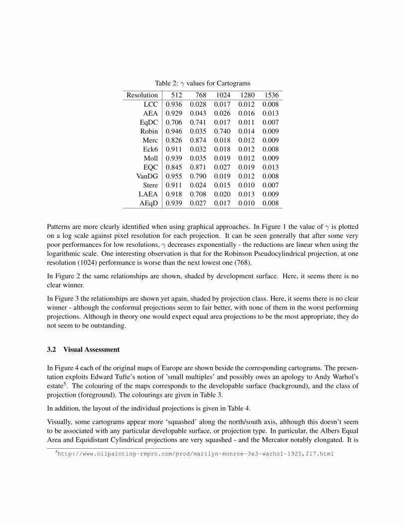
Table 2: γ values for Cartograms

Resolution 512 768 1024 1280 1536LCC 0.936 0.028 0.017 0.012 0.008AEA 0.929 0.043 0.026 0.016 0.013

EqDC 0.706 0.741 0.017 0.011 0.007Robin 0.946 0.035 0.740 0.014 0.009Merc 0.826 0.874 0.018 0.012 0.009Eck6 0.911 0.032 0.018 0.012 0.008Moll 0.939 0.035 0.019 0.012 0.009EQC 0.845 0.871 0.027 0.019 0.013

VanDG 0.955 0.790 0.019 0.012 0.008Stere 0.911 0.024 0.015 0.010 0.007

LAEA 0.918 0.708 0.020 0.013 0.009AEqD 0.939 0.027 0.017 0.010 0.008

Patterns are more clearly identified when using graphical approaches. In Figure 1 the value of γ is plottedon a log scale against pixel resolution for each projection. It can be seen generally that after some verypoor performances for low resolutions, γ decreases exponentially - the reductions are linear when using thelogarithmic scale. One interesting observation is that for the Robinson Pseudocylindrical projection, at oneresolution (1024) performance is worse than the next lowest one (768).

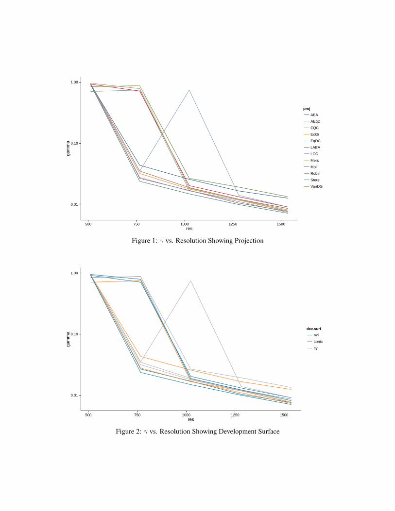
In Figure 2 the same relationships are shown, shaded by development surface. Here, it seems there is noclear winner.

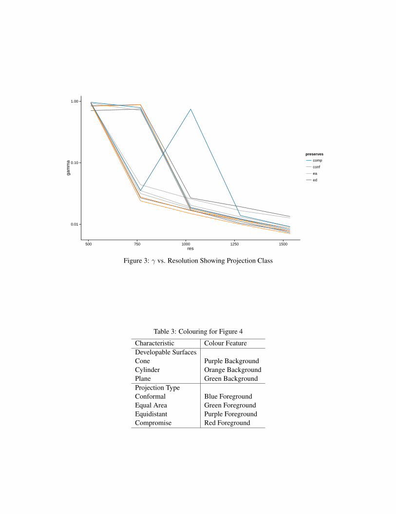
In Figure 3 the relationships are shown yet again, shaded by projection class. Here, it seems there is no clearwinner - although the conformal projections seem to fair better, with none of them in the worst performingprojections. Although in theory one would expect equal area projections to be the most appropriate, they donot seem to be outstanding.

3.2 Visual Assessment

In Figure 4 each of the original maps of Europe are shown beside the corresponding cartograms. The presen-tation exploits Edward Tufte’s notion of ’small multiples’ and possibly owes an apology to Andy Warhol’sestate5. The colouring of the maps corresponds to the developable surface (background), and the class ofprojection (foreground). The colourings are given in Table 3.

In addition, the layout of the individual projections is given in Table 4.

Visually, some cartograms appear more ‘squashed’ along the north/south axis, although this doesn’t seemto be associated with any particular developable surface, or projection type. In particular, the Albers EqualArea and Equidistant Cylindrical projections are very squashed - and the Mercator notably elongated. It is

5http://www.oilpainting-repro.com/prod/marilyn-monroe-3x3-warhol-1925,217.html

0.01

0.10

1.00

500 750 1000 1250 1500res

gam

ma

proj

AEA

AEqD

EQC

Eck6

EqDC

LAEA

LCC

Merc

Moll

Robin

Stere

VanDG

Figure 1: γ vs. Resolution Showing Projection

0.01

0.10

1.00

500 750 1000 1250 1500res

gam

ma

dev.surf

azi

conic

cyl

Figure 2: γ vs. Resolution Showing Development Surface

0.01

0.10

1.00

500 750 1000 1250 1500res

gam

ma

preserves

comp

conf

ea

ed

Figure 3: γ vs. Resolution Showing Projection Class

Table 3: Colouring for Figure 4

Characteristic Colour FeatureDevelopable SurfacesCone Purple BackgroundCylinder Orange BackgroundPlane Green BackgroundProjection TypeConformal Blue ForegroundEqual Area Green ForegroundEquidistant Purple ForegroundCompromise Red Foreground

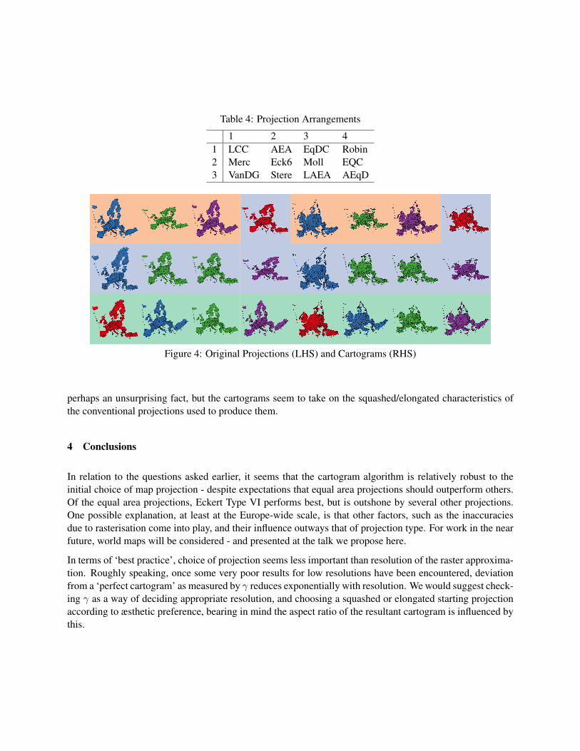
Table 4: Projection Arrangements

1 2 3 41 LCC AEA EqDC Robin2 Merc Eck6 Moll EQC3 VanDG Stere LAEA AEqD

Figure 4: Original Projections (LHS) and Cartograms (RHS)

perhaps an unsurprising fact, but the cartograms seem to take on the squashed/elongated characteristics ofthe conventional projections used to produce them.

4 Conclusions

In relation to the questions asked earlier, it seems that the cartogram algorithm is relatively robust to theinitial choice of map projection - despite expectations that equal area projections should outperform others.Of the equal area projections, Eckert Type VI performs best, but is outshone by several other projections.One possible explanation, at least at the Europe-wide scale, is that other factors, such as the inaccuraciesdue to rasterisation come into play, and their influence outways that of projection type. For work in the nearfuture, world maps will be considered - and presented at the talk we propose here.

In terms of ‘best practice’, choice of projection seems less important than resolution of the raster approxima-tion. Roughly speaking, once some very poor results for low resolutions have been encountered, deviationfrom a ‘perfect cartogram’ as measured by γ reduces exponentially with resolution. We would suggest check-ing γ as a way of deciding appropriate resolution, and choosing a squashed or elongated starting projectionaccording to æsthetic preference, bearing in mind the aspect ratio of the resultant cartogram is influenced bythis.

5 Acknowledgements

We gratefully acknowledge support from the ESPON Programme under the Multidimensional DatabaseDesign and Development (M4D) Project. Text and maps stemming from research projects under the ESPONProgram presented here do not necessarily reflect the opinion of the ESPON Monitoring Committee.

6 Biography

Chris Brunsdon is Professor of Geocomputation and Director of Maynooth University National Centre forGeocomputation. His research interests involve spatial statistics, visualisation and geocomputation appliedto a number of areas, including crime pattern analysis, and the analysis of environmental data.

Martin Charlton is a Senior Research Fellow and Deputy Director of Maynooth University National Centrefor Geocomputation. His research interests involve geographical information systems, data analysis and geo-computation applied to a number of areas, including health data, and the analysis of housing data data.

Both Chris and Martin played roles in the development of Geographically Weighted Regression, and areactively involved in developing and implementing tools for this and related techniques in the R programminglanguage.

References

Bugayevskiy, L. and Snyder, J. (1995). Map projections. A Reference Manual. Taylor and Francis, London.

Dorling, D. (1996). Area cartograms: their use and creation. Number 59 in CATMOG: Concepts andTechniques in Modern Geography.

Gastner, M. T. and Newman, M. E. (2004). Diffusion-based method for producing density-equalizing maps.Proceedings of the National Academy of Sciences of the United States of America, 101(20):7499–7504.

Sagar, B. D. (2013). Cartograms via mathematical morphology. Information Visualization, 13(1):42–58.

Tobler, W. R. (1973). A continuous transformation useful for districting. Annals New York Academy ofSciences, 219:215–220.