ssn college of engineering, kalavakkam, chennai arxiv:2108

Wind Power Projection using Weather Forecastsby Novel Deep Neural Networks

Alagappan Swaminathan1?, Venkatakrishnan Sutharsan1 ? and TamilselviSelvaraj2

1 SSN College of Engineering, Kalavakkam, Chennai{alagappan16011, venkatakrishnansutharsan16119}@eee.ssn.edu.in,2 Associate Professor, SSN College of Engineering, Kalavakkam, Chennai

[email protected]

Abstract. The transition from conventional methods of energy pro-duction to renewable energy production necessitates better predictionmodels of the upcoming supply of renewable energy. In wind power pro-duction, error in forecasting production is impossible to negate owingto the intermittence of wind. For successful power grid integration, itis crucial to understand the uncertainties that arise in predicting windpower production and use this information to build an accurate andreliable forecast. This can be achieved by observing the fluctuations inwind power production with changes in different parameters such as windspeed, temperature, and wind direction, and deriving functional depen-dencies for the same. Using optimized machine learning algorithms, it ispossible to find obscured patterns in the observations and obtain mean-ingful data, which can then be used to accurately predict wind powerrequirements . Utilizing the required data provided by the Gamesa’swind farm at Bableshwar, the paper explores the use of both parametricand the non-parametric models for calculating wind power predictionusing power curves. The obtained results are subject to comparison tobetter understand the accuracy of the utilized models and to determinethe most suitable model for predicting wind power production based onthe given data set.

Keywords: NWP, CERC, ANN, Linear Regression, Polynomial Regression,MAE, RMSE, R Square

1 Introduction

Wind energy is undoubtedly one of the most fundamental pillars that supportsthe growth of mankind. It is the sustenance of modern economies and the key forglobal progress. For generations, the demand for wind energy has been met byconventional sources of energy: oil, coal, and petroleum.The widespread heavyusage of these non-renewable sources is accompanied by several concerns. Firstly,

? Equal Contribution

arX

iv:2

108.

0979

7v1

[cs

.LG

] 2

2 A

ug 2

021

2 Alagappan et al.

the most pressing consequence of the burning of fossil fuels is the growing cli-mate crisis. The extraction as well as combustion of conventional energy sourcesresults in the emission of greenhouse gases and pollutants which, in turn, im-pacts the air quality, contributes to global warming, and causes damage to thesurrounding environment. In addition, the heavy reliance of global economies onfossil fuels for energy is cause for worry; since these sources are non-renewable,increased usage will eventually lead to their depletion, leaving the energy secu-rity of developed and developing nations to hang in the balance and restrictingtheir energy independence. These environmental and public health concerns arefurther exacerbated by a rapidly growing population, improvements in standardsof living, and increased industrialization which will cause a massive increase inthe energy demand.

2 Literature Survey

2.1 Wind Power in India

India is relatively a newcomer to the global wind power market, compared toDenmark and the United States of America (USA). However, the growth of windpower in India in recent times has been tremendous, ranking the Indian windpower market as the fourth largest in the world after China, USA, and Germany,and the second largest wind power market in Asia. The leader in wind powerin India is Tamil Nadu, with a wind power capacity that is approximately 29%of the national total. The largest wind power plant in India is the Muppandalwind farm, which has a total capacity of 1500 MW.

2.2 Indian Electricity Grid Code Requirements

In India, the regulatory body of the power sector is the Central Electricity Reg-ulatory Commission (CERC). The CERC has established regulations for powersystem operations known as the IEGC.According to these requirements, everywind farm with aggregate generation capacity of 50 MW and above must per-form wind energy forecast with an interval of 15 minutes for the next 24 hours.In order to ensure that the forecasting models are aligned to minimize the ac-tual MW deviations, CERC defines the percentage error normalized to the ratedcapacity of the plant. Wind farm operators are allowed to submit a total of 8revisions throughout the day, up to 3 hours before the actual schedule. In doingso, the forecast is improved; as more data becomes available, forecast errors areminimized, consequently reducing economic losses.

2.3 Available Prediction Methods

Numerous models have been identified for the crucial task of predicting windpower production, each having its own characteristics. The performance of eachmodel is dependent upon the nature of the data it is trained with, which is mostly

Deep Neural Network for Power Prediction 3

site-specific. Thus, the accuracy of prediction of wind power production in aparticular region or for a particular wind farm relies on selecting the appropriatemodel to perform the task The performance of each model is dependent uponthe nature of the data it is trained with, which is mostly site-specific. Thus, theaccuracy of prediction of wind power production in a particular region or for aparticular wind farm relies on selecting the appropriate model to perform thetask.

The models which are currently available include:

– Persistence Method– Numerical Weather Prediction Methods– Statistical and Neural Network Methods

2.4 Persistence Method

The persistence method operates on the simple assumption that the wind speedor wind power at a certain time in the future will be the same as it was whenthe forecast was made. In other words, this model assumes a high correlationbetween the present and future wind values. The persistence method is notonly the simplest and most economical, but also more accurate than other windforecasting methods - but only in ultra-short-term forecasting. This method isused in electrical utility for ultra-short-term forecasts. But its accuracy degradesrapidly as the time-scale of forecasting increases.[5]

2.5 Numerical Weather Prediction Methods

This is a classical forecasting technique. Numerical Weather Prediction (NWP)models operate by solving conservation equations (mass, momentum, heat, wa-ter, etc.) numerically at given locations on a spatial grid. Future behaviour ofthe atmosphere is predicted using current conditions and past trends. This tech-nique is based on the topology and layout of the wind farms, specifications ofthe wind turbines, and numerical weather predictions updated by meteorologicalservices along with data from a large number of sources.[6]

When attempting the task of prediction using a NWP model, the most criti-cal step is the selection of the particular NWP model. There are several criteriawhich must be taken into consideration when making this choice: the geograph-ical area, the resolution (both spatial and temporal), the forecast horizon, theaccuracy required, the computation time, and the number of runs. The focusof research on prediction methods, until recently, has been NWP models. Thisis mainly because NWP models are dominant for long-term forecasting (severalhours to days ahead).

However, it is important to note that these models are incredibly complexand take several hours to obtain a solution on a super computer. In addition,NWP models are also susceptible to inflicting uncertainties which can affectthe accuracy of prediction. These uncertainties arise from model assumptionsof initial conditions of the atmosphere, adopted parameterization methods, and

4 Alagappan et al.

post-processing techniques which do not always replicate the real-time condi-tions. Additionally, these assumptions inherently generalize the state of the at-mosphere, which often ignores the local phenomenon and weather variability.These uncertainties eventually influence the performance of the prediction modelat a regional scale. For short-term prediction models, therefore, NWP modelsare not preferred[7].

2.6 Statistical and Neural Network Methods

This method relies on learning from historical data. A vast amount of data isanalyzed and meteorological processes are not explicitly represented. Instead, alink between the power produced in the past and the weather during those timeperiods is determined. This is then utilized for predicting the future output. Themodel is generally represented as a time series model or a dynamic model whoseparameters are estimated by minimizing a cost function over historical trainingdata set.

There are several techniques which are classified as statistical methods ofprediction. Some of the most common are the Box-Jenkins methodology, au-toregressive (AR), moving average (MA), the autoregressive integrated movingaverage model (ARIMA), autoregressive moving average model (ARMA), andthe use of the Kalman filter. These methods model the statistical relationshipamong the historical data using classical time series analysis. Soft computingand machine learning approaches such as regression algorithms, , ANN, andsupport vector machine (SVM), to name a few, also come under this category.In particular, Foley et al. describe the approach of using ANNs as a data-drivenapproach[8]. Before arriving at a selection of models to be studied in this report,the usage of prediction techniques in other studies was investigated.

Torres et al. obtained a 20% error reduction compared to persistence toforecast average hourly wind speed for a 10 hour forecast at a number of locationsusing nine years of historical dating using an ARMA model[9]. Using ARIMAmodels, Kavasseri and Seetharaman took significantly longer prediction horizonsinto account and predicted wind speeds of 1-day-ahead and 2-day-ahead periods,respectively. Through this method, the forecasting accuracy was improved by anaverage of 42% compared to the persistence method. In doing so, they highlightedthe necessity of scheduling dispatchable generation and tariffs in the day-aheadelectricity market[10]. Additionally, Lei and Ran presented a hybrid model basedon wavelet-decomposition and ARMA for short-term wind speed prediction fora wind farm[11].

In Brazil, Lira et al. relied on linear regression to predict wind speeds at threedifferent altitudes in two different geographical areas, Paracuru and Camocim,describing spatial relationships of wind speed data between these two sites.The results of this approach demonstrated the strength of simple regressionmethods[12]. On the other hand, a study performed by Kafazi et al. found poly-nomial curve fitting model to be a better choice for forecasting energy productionapplications[13].


Techniques such as ANNs and Neuro-fuzzy networks have been used increas-ingly in recent times. In a comprehensive comparison study on the application ofadaptive linear element, back propagation, and radial basis function type neuralnetworks, Li and Shi applied ANNs in 1-hour-ahead wind speed forecasting[14].In a comparative analysis of three types of neural networks, namely multi-layerperceptron (MLP), simultaneous recurrent neural network (SRN), and Elmanrecurrent neural network, which were trained using particle swarm optimiza-tion(PSO), Welch et al. performed short-term prediction of wind speed[15]. Ad-ditionally, Jursa and Rohrig presented an approach combining ANN and nearest-neighbor approaches in an optimization model[16].

Statistical methods work best for short-term models, the reason being thatforecasting errors could get accumulated quickly with increasing prediction hori-zons. It is also important to note that these models are not portable; they requirethe assistance of a domain expert to create an individualized model for each windfarm. Since there is a lack of portability, changes in weather conditions wouldwarrant significant changes in the model itself, which in turn would require theattention of an expert for re-tuning the parameters of the statistical model[17].

3 Novelty

The Novel approach taken in this paper is to use other parameters which arewind direction and temperature to assist wind speed in predicting the outputpower. The major improvements are shown in R-Squared value which is a keyparameter for prediction analysis which is basically the goodness of fit measurefor learning models. The average R-Squared value of our predicted Linear Re-gression model is around 0.8708% which is very high compared to R-Squaredvalue of 0.692%[13]. Also, the Polynomial Regression of 5th order prove to be abetter model with maximum R-Squared value of 0.96435% compared to 0.9342%using 2nd degree Polynomial Regression by Kafazi et al[13]. The Artificial Neu-ral Network has shown an average R-Squared Value of 0.966075% which is thebest in this comparison. The Artificial Neural Network with Wind speed and di-rection as input has shown better learning compared to ANN with wind speed,direction and temperature as input indicating the minimal effect of temperatureof wind in Wind Power Forecasting. Thus this novel approach has been provedto be better in performance compared to the other existing methods.

4 Experimentation

4.1 Wind Power Prediction using Power Curve

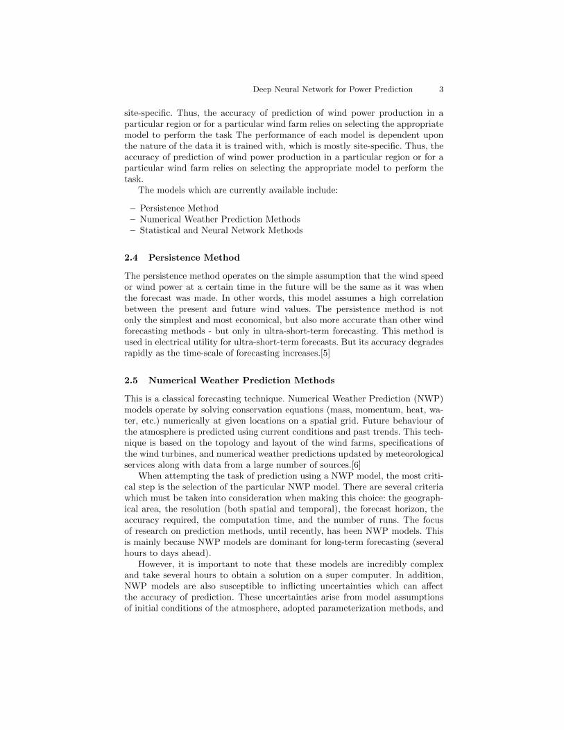
Before predicting wind power outputs, it is necessary to analyze power curves asthey represent characters of wind turbine outputs. A power curve represents therelationship between the wind speed and the output power of a turbine. For aparticular turbine, the power curve is provided by the turbine manufacturer. It

6 Alagappan et al.

is used for energy assessment and for monitoring the performance of the turbine.The Fig. 1 represents a typical power curve of a wind turbine.

Also we know the relation between the power generated and the wind speedto be known by

P = 0.5ρCpAV3 (1)

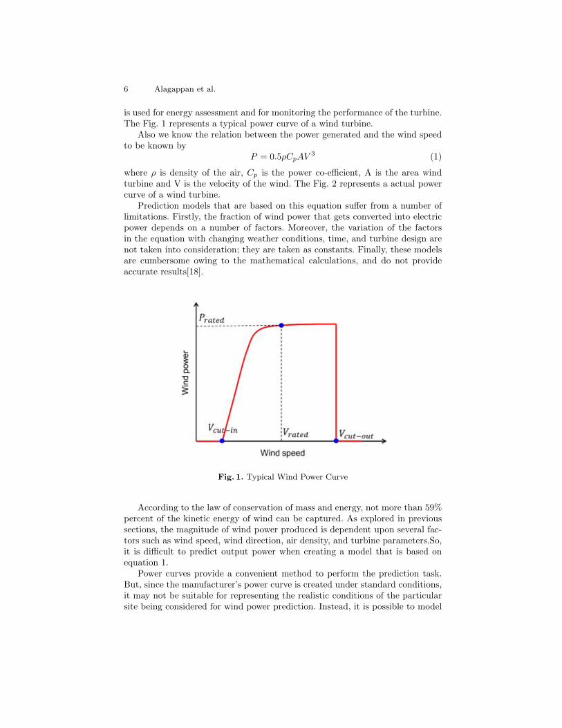
where ρ is density of the air, Cp is the power co-efficient, A is the area windturbine and V is the velocity of the wind. The Fig. 2 represents a actual powercurve of a wind turbine.

Prediction models that are based on this equation suffer from a number oflimitations. Firstly, the fraction of wind power that gets converted into electricpower depends on a number of factors. Moreover, the variation of the factorsin the equation with changing weather conditions, time, and turbine design arenot taken into consideration; they are taken as constants. Finally, these modelsare cumbersome owing to the mathematical calculations, and do not provideaccurate results[18].

Fig. 1. Typical Wind Power Curve

According to the law of conservation of mass and energy, not more than 59%percent of the kinetic energy of wind can be captured. As explored in previoussections, the magnitude of wind power produced is dependent upon several fac-tors such as wind speed, wind direction, air density, and turbine parameters.So,it is difficult to predict output power when creating a model that is based onequation 1.

Power curves provide a convenient method to perform the prediction task.But, since the manufacturer’s power curve is created under standard conditions,it may not be suitable for representing the realistic conditions of the particularsite being considered for wind power prediction. Instead, it is possible to model


Fig. 2. Actual Representation of the Wind Power Curve

power curves by deriving them using the actual data of wind speed and outputpower of the turbine, which makes the prediction more accurate[19].

Models can be classified as Parametric and Non-Parametric Models on thebasis of the power curve.

4.2 Parametric and Non-Parametric Models

In parametric models, the relationship between the input and output, or thedependent and independent variable, is known. They are built from a set ofmathematical equations that include parameters that must be adapted througha set of continuous data[21]. The parameter values may be unknown, and are es-timated from the training set. With developments in soft computing techniques,newer modelling methods have emerged known as learning methods. These areclassified as non-parametric methods. Here, instead of assuming a physical oranalytical relationship between the input and output data, a correlation is es-tablished based only on the data provided.An example of this would be ANNs,the use of which in predicting wind power production has been explored in thispaper. In the extensive literature surveyed, none of the authors ever modelled apower curve with more than three inputs simultaneously.

4.3 Linear Regression

Linear regression is one of the most fundamental algorithms used for predictiveanalysis. It is utilized for determining a relationship between one dependentvariable and one or more independent variables. By using this algorithm, weaim to obtain the best fit line or regression equation that can be used to makeaccurate predictions. One of the main advantages of using linear regression is itssimplicity. This algorithm can be used to determine the strength of the factors

8 Alagappan et al.

being considered for prediction, conduct predictive analysis, and forecast trends.Yang et al. have proposed a linear regression based model for power predictionin which output power increases linearly.

As the name suggests, linear regression assumes a linear relationship betweenthe input variables, say xi, and the output variable, say y. This algorithm sug-gests that y can be calculated from a linear combination of input variables. Inthe linear equation formed, each input value is assigned a scale factor or coeffi-cient. Additionally, another coefficient β0 is included in the equation to providean additional degree of freedom. In a simple regression problem, i.e., with asingle input and output, the linear regression model would be expressed by thefollowing equation:

y = β0 + β1 ∗ x1 + ε (2)

where y is the output value, β0 the bias term, β1 is the slope coefficient, xiis the independent variable, and ε is a random error term.

The above representation simplifies the process of predicting output values fora given set of input values. For training the equation from data, there are severaltechniques which can be employed. Here, the Ordinary Least Squares methodhas been used for optimization and to minimize error. There is a problem ofover-fitting which is predominantly due to increase in number of features givingrise to higher order polynomial equation.

4.4 Polynomial Regression

With linear regression, we attempt to find a linear relationship between the de-pendent variable and one or more independent variables. But, in many cases, thedistribution of the data set is far more complex, and this linear model cannot beutilized efficiently to fit the data; doing so with a low value of error is incrediblydifficult. Therefore, in these cases, it becomes a necessity to increase the com-plexity of the model. Polynomial regression is a predictive modelling techniquewherein we attempt to fit a polynomial line in accordance with the non-linearrelationship between the output variable and one or more input variables. It hasbeen extensively used in literature to estimate the power curve of wind turbines.Shokrzadeh et al. proposed a polynomial regression based model for power pre-diction, where the relationship between the dependent and independent variablesis curvilinear. The general equation of a polynomial regression model is:

y = β0 + β1 ∗ x1 + β2 ∗ x2 + ......+ βm ∗ xm + ε (3)

One of the advantages of using this algorithm is that a broad range of func-tions can be fit under it. However, it is sensitive to outliers; the presence of evenone or two outliers in the data set can impact the results determined from thenon-linear analysis.


4.5 Artificial Neural Network

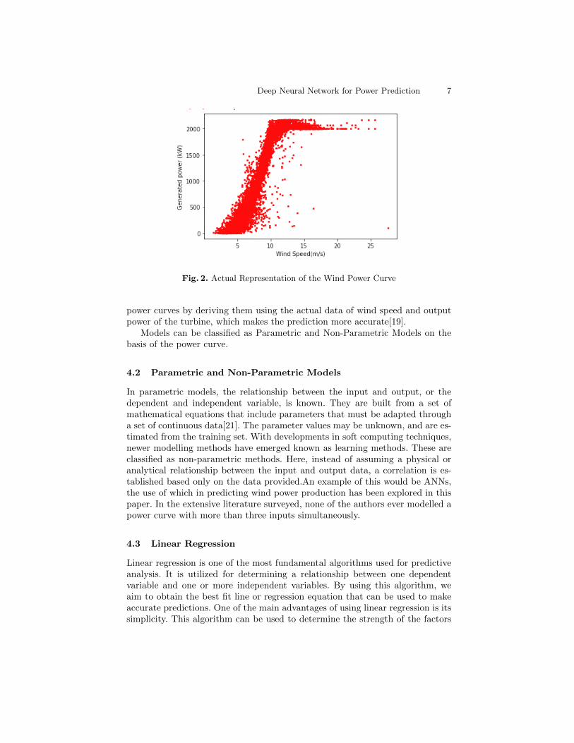
The working of ANN is inspired by biological nervous systems. ANNs are de-signed to imitate the working of the human brain. This is to determine thenon-linear relationships between the input and the output data sets. Similarto the human brain, the fundamental building block of an ANN is the neuron,the structure of which is shown in Fig. 3. Each neuron has an input signal Xj

which it alters and sends forward. Each neuron is interconnected to another viaweighted synapses which decide the strength of the connection to the next step.The next step is the summing junction which adds the weighted input signals ofthe neuron. The output of the neuron is then limited using an activation functionΦ which limits the output to a set finite range and returns an output. This canbe expressed as:

Yk = φ(uk + bk) (4)

Fig. 3. Neuron of an ANN

The proposed ANN model in this report is a feed-forward neural networkwith an input layer, an output layer, and four hidden layers. A sample structureof an ANN with multiple hidden layers is shown in Fig. 4. Further, two kinds ofactivation functions were utilized: Sigmoid and ReLU. Sigmoid functions allowfor a smooth gradient, normalizing the output of each neuron in the ANN. Usingthe ReLU activation function makes the network more computationally efficient,allowing the network to converge very quickly. These activation functions weresuitable here as the data to be processed as well as the expected outcome werenot negative values. In general, there are several advantages in using ANNs.The key advantage of an ANN is its ability to learn and model non-linear andcomplex relationships. This makes ANNs suitable for capturing the non-linearityof the wind speed characteristic. After training, ANNs are capable of inferringunseen relationships, thus making the model generalize and predict on unseendata.

10 Alagappan et al.

Fig. 4. General structure of an ANN with multiple hidden layers

Additional advantages of an ANN are its ability to work with incompleteknowledge and its fault tolerance. After training the ANN, the network mayproduce an output even if some of the information is incomplete; the loss ofperformance depends on the importance of the missing information. However,a disadvantage of using an ANN is its black-box approach; it is difficult tounderstand the exact internal working of the ANN, rendering its behaviour un-explained. This reduces trust in the network. In addition, there is no specific rulefor determining the structure of an ANN; the appropriate structure is determinedthrough trial and error.

5 Evaluation of Models

It is difficult to accurately measure the performance of different prediction mod-els merely by comparing their output plots. Hence, in this report, the perfor-mance of the proposed models have been quantified using the following evalua-tion metrics:

– Mean Absolute Error (MAE)– Root Mean Square Error(RMSE)– R Squared Value

5.1 Mean Absolute Error

The MAE is defined as the average of the difference between the predicted andactual values in the test - in other words, the average prediction error. It isexpressed as in equation 5.

MAE = 1/N ∗N∑i=1

|pi − ppredictedi | (5)

Where ppredictedi is the power output and pi is the actual power output attime i, respectively, and N is the number of forecast samples.


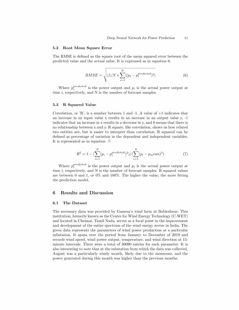
5.2 Root Mean Square Error

The RMSE is defined as the square root of the mean squared error between thepredicted value and the actual value. It is expressed as in equation 6.

RMSE =

√√√√(1/N ∗N∑i=1

|(pi − ppredictedi )2| (6)

Where ppredictedi is the power output and pi is the actual power output attime i, respectively, and N is the number of forecast samples.

5.3 R Squared Value

Correlation, or ’R’, is a number between 1 and -1. A value of +1 indicates thatan increase in an input value x results in an increase in an output value y, -1indicates that an increase in x results in a decrease in y, and 0 means that there isno relationship between x and y. R square, like correlation, shows us how relatedtwo entities are, but is easier to interpret than correlation. R squared can bedefined as percentage of variation in the dependent and independent variables.It is represented as in equation 7.

R2 = 1− (

N∑i=1

(pi − ppredictedi )2)/(

N∑i=1

(pi − pmean)2) (7)

Where ppredictedi is the power output and pi is the actual power output attime i, respectively, and N is the number of forecast samples. R squared valuesare between 0 and 1, or 0% and 100%. The higher the value, the more fittingthe prediction model.

6 Results and Discussion

6.1 The Dataset

The necessary data was provided by Gamesa’s wind farm at Bableshwar. Thisinstitution, formerly known as the Centre for Wind Energy Technology (C-WET)and located in Chennai, Tamil Nadu, serves as a focal point in the improvementand development of the entire spectrum of the wind energy sector in India. Thegiven data represents the parameters of wind power production at a particularsubstation. It spans over the period from January to December of 2019 andrecords wind speed, wind power output, temperature, and wind direction at 15-minute intervals. There were a total of 30090 entries for each parameter. It isalso interesting to note that at the substation from which the data was collected,August was a particularly windy month, likely due to the monsoons, and thepower generated during this month was higher than the previous months.

12 Alagappan et al.

6.2 Impact of Wind speed, Wind direction and Temperature onWind power production

For the prediction of wind power production, three factors have been takeninto consideration: wind speed, wind direction, and temperature. Before usingthe respective data to train the proposed models, the extent of the influence ofthese parameters on wind power production was first explored. Fig. 5 presents amatrix-like correlation, relaying the extent to which wind speed, wind direction,and temperature are correlated to each other and the generated wind power,based on the data provided by Gamesa’s wind farm at Bableshwar. The greaterthe value at the intersection of two parameters, the more inter-related are thetwo parameters; the maximum value of correlation is 1. As explored in previoussections, wind power production is highly dependent upon wind speed. Thisrelationship is reflected in Fig. 5, with a value of 0.934438 at their intersection.We can also see that wind direction and temperature have a negligible impact onwind power production as the corresponding values in the figure are incrediblylow. This information provided by Fig. 5 can also be represented visually bymeans of a heat map.

Fig. 5. Correlation of the effects of wind speed, wind direction, and temperature onwind power production

Fig. 6, which has been generated using Python, represents the correlationbetween any two of the considered parameters using the colour of the tile at theintersection of two parameters. As per the colour scale provided in the figure, alighter colour represents greater correlation and a darker colour represents negli-gible correlation. Here, too, we see the great influence of wind speed upon windpower production and the negligible effect of wind direction and temperature onwind power production. Nevertheless, wind direction and temperature have beentaken into consideration for training the proposed models in order to analyze theimpact of these parameters in reducing the error of prediction.

6.3 Linear Regression

It establishes a linear relationship between the dependent and independent vari-ables.First, the necessary Python libraries were imported. Then, the given dataset was loaded. The data set contains all the values in the form of a table. Vari-ables X and y were trained with data from the relevant columns of the data


Fig. 6. Heatmap to visually represent the correlation matrix

table. By setting the value of ’test size’, we were able to vary the proportion ofthe data set being used for training and testing the model.The ’random state’parameter was used to randomize the splitting of the data into train and testindices. Following this, a linear regression object was created. The correspondingMAE, RMSE, and R squared values were then calculated.

Fig. 7. Power curve fitting when the proposed linear regression model is trained using85% of the given data

Fig. 7 was plotted using 85% of the given data when considering wind speed,wind direction, and temperature.Given that this is a linear regression model,the expected relationship between wind power production and the influencingparameters was also linear. This is confirmed by the interpretation of Fig. 7. Itcompares the power curve that corresponds to the predicted values of generated

14 Alagappan et al.

power and wind speed with the power curve that corresponds to the actualvalues of generated power and wind speed. The scattered red region representsthe actual values plotted between wind speed and wind power, and the blueline represents the power curve for the predicted value. Clearly, the power curvecorresponding to the predicted values does not fit well against the power curvecorresponding to the actual values. From this figure, one can interpret that theaccuracy of the proposed linear regression model is dismal for the given data set.

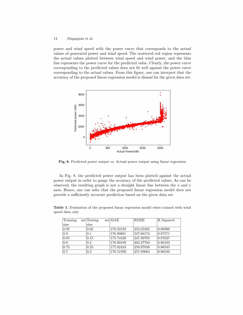
Fig. 8. Predicted power output vs. Actual power output using linear regression

In Fig. 8, the predicted power output has been plotted against the actualpower output in order to gauge the accuracy of the predicted values. As can beobserved, the resulting graph is not a straight linear line between the x and yaxes. Hence, one can infer that the proposed linear regression model does notprovide a sufficiently accurate prediction based on the given data set.

Table 1. Evaluation of the proposed linear regression model when trained with windspeed data only

Training setsize

Testing setsize

MAE RMSE R Squared

0.95 0.05 178.33192 253.35265 0.86980

0.9 0.1 176.90861 247.66174 0.87571

0.85 0.15 175.74426 247.39705 0.87627

0.8 0.2 176.90189 262.27704 0.86103

0.75 0.25 177.02434 259.97856 0.86345

0.7 0.3 176.51930 257.89664 0.86533


Table 2. Evaluation of the proposed linear regression model when trained with windspeed and wind direction data only

Training setsize

Testing setsize

MAE RMSE R Squared

0.95 0.05 178.81581 253.11586 0.87107

0.9 0.1 177.40251 246.68685 0.87668

0.85 0.15 176.37347 246.52254 0.87714

0.8 0.2 177.55531 261.27449 0.86209

0.75 0.25 177.90095 258.99536 0.86448

0.7 0.3 177.42095 256.85976 0.866411

Table 3. Evaluation of the proposed linear regression model when trained with windspeed and temperature data only

Training setsize

Testing setsize

MAE RMSE R Squared

0.95 0.05 175.36880 250.02119 0.87320

0.9 0.1 173.18357 243.63749 0.87971

0.85 0.15 172.45955 243.95124 0.87969

0.8 0.2 173.64332 258.94650 0.86453

0.75 0.25 173.98111 256.71224 0.86686

0.7 0.3 173.52368 254.57559 0.86877

Table 4. Evaluation of the proposed linear regression model when trained with windspeed, wind direction, and temperature data

Training setsize

Testing setsize

MAE RMSE R Squared

0.95 0.05 175.84133 249.02472 0.87421

0.90 0.10 173.62791 242.88975 0.88045

0.85 0.15 173.08321 243.29391 0.88034

0.80 0.20 174.29879 258.14871 0.86537

0.75 0.25 174.82482 255.90645 0.86769

0.70 0.30 174.40050 253.70599 0.86967

16 Alagappan et al.

The first column of each table namely TABLE 1, TABLE 2, TABLE 3, TA-BLE 4 represents the fraction of the data set which was used to train the model.The values in this column vary from 0.95 to 0.7 in decrements of 0.05. Thesecond column represents the fraction of the data set which was used for vali-dating the values predicted by the model. The last three columns represent thecorresponding MAE, RMSE, and R squared values which were considered forevaluating the performance of the model.The evaluation metrics confirm thatthe accuracy of the proposed linear regression model is not impressive; whilethe R squared value is above 0.8 under all conditions, a more reliable predictionmodel is certainly preferable. Further, if one observes the variation in the valuesof the evaluation columns, one can notice that the best values, i.e., least error,is obtained when the training set size is 0.85.So, for the particular sub-stationtaken into consideration and for the corresponding data set, the proposed linearregression model works best with a training set size ranging from 0.85 to 0.9when trained with wind speed, wind direction, and temperature data.

6.4 Polynomial Regression

With the proposed polynomial regression model, the expectation is to obtain apower curve from the predicted values which fits closer to the actual power curve,unlike the proposed linear regression model. When using polynomial regression,one accounts for the complexity of the distribution of a particular data set.So, with the proposed polynomial regression model, the non-linear relationshipbetween dependent and independent variables is accounted for. The data setcontains all the values in the form of a table. Variables X and y were trained withdata from the relevant columns of the data table. By setting the value of ’testsize’, we were able to vary the proportion of the data set being used for trainingand testing the model. The ’random state’ parameter was used to randomizethe splitting of the data into train and test indices. Then, a polynomial featuresobject was created, followed by a linear regression object. Since the degree ofthe polynomial also influences the accuracy, the degree of the polynomial wasvaried.

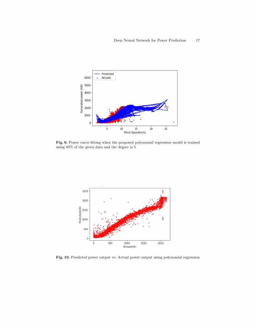
This value can vary from 2 to (n-1), where n is the number of data points.The corresponding MAE, RMSE, and R squared values were then calculatedand printed. Fig. 9 was then plotted,using 85% of the given data when consid-ering wind speed, temperature, and wind direction. Since this is a polynomialregression model, the expected relationship between wind power production andthe influencing parameters is non-linear. This is reflected in Fig. 9 which com-pares the power curve corresponding to the predicted values - a sigmoid curve- with that of the actual values. Clearly, one can observe that the power curvecorresponding to the predicted values fits much better with the actual powercurve than the proposed linear regression model. From this, one can deduce thatthe accuracy of prediction of the proposed polynomial regression model is muchgreater than that of the proposed linear regression model.

In Fig. 10, the predicted power output has been plotted against the actualpower output in order to gauge the accuracy of the predicted values. As can


Fig. 9. Power curve fitting when the proposed polynomial regression model is trainedusing 85% of the given data and the degree is 5

Fig. 10. Predicted power output vs. Actual power output using polynomial regression

18 Alagappan et al.

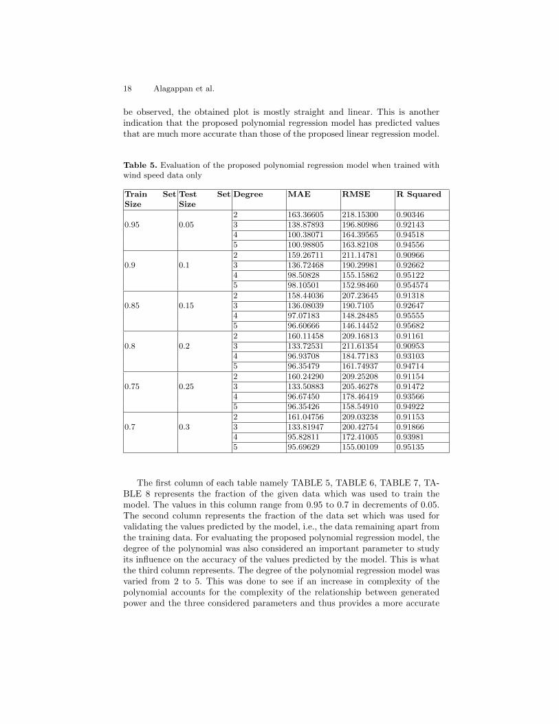
be observed, the obtained plot is mostly straight and linear. This is anotherindication that the proposed polynomial regression model has predicted valuesthat are much more accurate than those of the proposed linear regression model.

Table 5. Evaluation of the proposed polynomial regression model when trained withwind speed data only

Train SetSize

Test SetSize

Degree MAE RMSE R Squared

2 163.36605 218.15300 0.903460.95 0.05 3 138.87893 196.80986 0.92143

4 100.38071 164.39565 0.945185 100.98805 163.82108 0.94556

2 159.26711 211.14781 0.909660.9 0.1 3 136.72468 190.29981 0.92662

4 98.50828 155.15862 0.951225 98.10501 152.98460 0.954574

2 158.44036 207.23645 0.913180.85 0.15 3 136.08039 190.7105 0.92647

4 97.07183 148.28485 0.955555 96.60666 146.14452 0.95682

2 160.11458 209.16813 0.911610.8 0.2 3 133.72531 211.61354 0.90953

4 96.93708 184.77183 0.931035 96.35479 161.74937 0.94714

2 160.24290 209.25208 0.911540.75 0.25 3 133.50883 205.46278 0.91472

4 96.67450 178.46419 0.935665 96.35426 158.54910 0.94922

2 161.04756 209.03238 0.911530.7 0.3 3 133.81947 200.42754 0.91866

4 95.82811 172.41005 0.939815 95.69629 155.00109 0.95135

The first column of each table namely TABLE 5, TABLE 6, TABLE 7, TA-BLE 8 represents the fraction of the given data which was used to train themodel. The values in this column range from 0.95 to 0.7 in decrements of 0.05.The second column represents the fraction of the data set which was used forvalidating the values predicted by the model, i.e., the data remaining apart fromthe training data. For evaluating the proposed polynomial regression model, thedegree of the polynomial was also considered an important parameter to studyits influence on the accuracy of the values predicted by the model. This is whatthe third column represents. The degree of the polynomial regression model wasvaried from 2 to 5. This was done to see if an increase in complexity of thepolynomial accounts for the complexity of the relationship between generatedpower and the three considered parameters and thus provides a more accurate


Table 6. Evaluation of the proposed polynomial regression model when trained withwind speed and wind direction data only

Train SetSize

Test SetSize


2 157.05884 209.08797 0.911320.95 0.05 3 131.54443 186.36933 0.92954

4 97.45729 158.21575 0.949225 95.88115 151.38449 0.95351

2 152.54157 200.85121 0.918250.9 0.1 3 128.39435 179.30980 0.93485

4 95.04405 151.07935 0.953755 92.51458 142.59749 0.95879

2 151.61996 196.97673 0.921560.85 0.15 3 127.66517 179.62605 0.93477

4 91.97351 141.40261 0.959585 90.24005 135.03130 0.96314

2 149.56589 194.20941 0.923800.8 0.2 3 124.87827 196.10105 0.92231

4 89.07193 172.24278 0.940065 88.52886 147.10882 0.95628

2 152.86237 198.26405 0.920580.75 0.25 3 124.56049 191.61831 0.92582

4 92.46087 170.92146 0.940985 90.32096 144.50929 0.95781

2 153.90863 198.8654 0.920070.7 0.3 3 124.96455 187.43514 0.92886

4 93.75799 171.02757 0.940775 90.21331 143.04789 0.95857

20 Alagappan et al.

Table 7. Evaluation of the proposed polynomial regression model when trained withwind speed and temperature data only

Train SetSize

Test SetSize


2 161.40320 214.77899 0.906430.95 0.05 3 136.60721 193.60344 0.92397

4 98.33635 161.14955 0.947325 98.18766 158.92774 0.94877

2 156.99932 207.33262 0.912890.9 0.1 3 133.73842 186.66654 0.92939

4 96.32098 151.98026 0.953195 95.5189 148.08611 0.95556

2 156.26280 203.63869 0.916170.85 0.15 3 133.73842 187.10393 0.92923

4 94.96499 144.78325 0.957625 94.20845 141.38741 0.95959

2 157.82921 205.42804 0.914740.8 0.2 3 130.82381 207.38387 0.91311

4 94.86253 189.62197 0.927365 94.00498 181.79505 0.93323

2 158.03800 205.65515 0.914550.75 0.25 3 130.71028 201.46466 0.91800

4 94.74571 182.64485 0.932615 94.07443 175.65365 0.93767

2 158.79705 205.48684 0.914500.7 0.3 3 131.07367 196.62502 0.92172

4 93.75628 175.81823 0.937415 93.17997 168.08954 0.94279


Table 8. Evaluation of the proposed polynomial regression model when trained withwind speed, wind direction, and temperature data

Train SetSize

Test SetSize


2 157.11845 208.03268 0.912210.95 0.05 3 131.45079 185.88187 0.92991

4 98.05413 158.74838 0.948885 93.73527 148.11939 0.95549

2 152.21444 199.90720 0.919020.9 0.1 3 128.37896 178.86032 0.93517

4 95.80909 151.64924 0.95395 90.57723 139.46847 0.96058

2 151.24862 196.21854 0.922160.85 0.15 3 127.38479 179.08433 0.93516

4 92.61943 141.62518 0.959455 88.83963 132.79841 0.96435

2 149.21291 193.62416 0.924260.8 0.2 3 124.83034 195.19840 0.92302

4 89.04671 182.19318 0.932945 87.45523 166.16806 0.944217

2 152.43461 197.55189 0.921160.75 0.25 3 124.48798 190.55189 0.92642

4 93.74098 181.54354 0.933425 89.02249 160.86614 0.94772

2 153.48259 197.94288 0.920670.7 0.3 3 124.91562 186.62300 0.92948

4 95.48558 181.98448 0.932945 88.21719 154.34707 0.95176

22 Alagappan et al.

result. The degree of the polynomial was not increased beyond 5 in order toavoid over-fitting the model and thus compromising the reliability of the model.The last three columns of the table explain the performance of the model interms of MAE, RMSE, and R squared values respectively. For every training setsize, the accuracy consistently increased with an increase in the degree of thepolynomial. The MAE and RMSE values decreased and the R squared valuesincreased with an increase in degree.

This indicates that lower degree polynomials were not ideal to represent thecomplexity of the relationship between generated wind power and the parame-ters taken into consideration, i.e., wind speed, wind direction, and temperature.So, one can observe that a fifth degree polynomial is best suited for accurateprediction using the proposed polynomial regression model. Further, under allfour testing conditions, the best R squared values were obtained when the de-gree of the polynomial was 5 and the training set size was 85% of the total datataken into consideration for each case. One can infer that a greater training setsize would have contributed to an increase in error, and a lesser training setsize would not have provided sufficient data for increased accuracy. The mostaccurate values predicted by the proposed polynomial regression value were ob-tained when the model was trained with wind speed, temperature data and winddirection, the training set size was 85% of the given data, and the degree was5; the R squared value under these conditions is 0.96435. This makes the pro-posed polynomial regression model much more suitable and reliable for the taskof predicting wind power output for the sub-station taken under considerationthan the previous model.

6.5 Artificial Neural Network

The ANN is a non-parametric model of predicting wind power production.Inthis proposed model, rather than defining the relationship between wind powerproduction and the considered parameters, the model is trained with the pro-vided data and the relationship between the dependent and independent factorsis derived by the model. This makes it much easier to establish a correlationbased on the provided data.Variables X and y were trained with data from therelevant columns of the data table. By setting the value of ’test size’, we wereable to vary the proportion of the data set being used for training and testingthe model. The ’random state’ parameter was used to randomize the splitting ofthe data into train and test indices. Then, an ANN with four hidden layers usingsigmoid and ReLu activation functions was created, compiled, trained with thegiven data, and tested. The corresponding MAE, RMSE, and R squared valueswere then calculated and printed. Fig. 11 was obtained using 85% of the givendata when considering wind speed, wind direction, and temperature.

Since ANNs have a black-box approach, making it difficult to understandthe inner workings of the network and the relationship established between theinput and output variables, the proposed feed-forward ANN model was createdby trial-and-error methods. In the process, it was found that a four-layered ANNwas optimal for the prediction task. Further, 20 epochs were found to be optimal


for training the proposed ANN model. One can infer here that a lesser number ofepochs would have resulted in under-fitting and more epochs would have causedover-fitting.

Fig. 11 provides a comparison between the power curve corresponding to thevalues predicted by the proposed ANN model and the actual power curve. Here,one can observe that the power curve corresponding to the predicted values is asigmoid graph and fits very close to the actual power curve - even better thanthat obtained with the proposed polynomial regression model. From this, onecan infer that the accuracy of prediction of the proposed ANN model is muchgreater than that of the proposed linear regression model and is likely to begreater than that of the proposed polynomial regression model.

Fig. 11. Power curve fitting using the proposed ANN model when trained with 85%of the given data

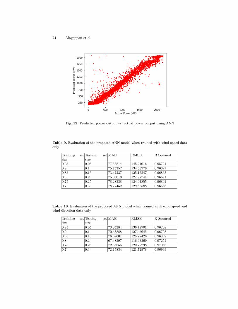
In Fig. 12, one can see the predicted power output plotted against the actualpower output. The graph is straight and linear - even more so than that obtainedfrom the proposed polynomial regression model, which is another indicator thatthe proposed ANN model is likely to have more accuracy than the polynomialregression model. This inference is substantiated by the following tables namelyTABLE 9, TABLE 10, TABLE 11, TABLE 12

Similar to the evaluation table corresponding to the proposed linear regres-sion model, the table has five columns. The first column represents the fractionof the data set which was used to train the model. The values in this columnvary from 0.95 to 0.7 in decrements of 0.05. The second column represents thefraction of the data set which was used for validating the values predicted bythe model. The last three columns represent the corresponding MAE, RMSE,and R squared which were considered for evaluating the model.

24 Alagappan et al.

Fig. 12. Predicted power output vs. actual power output using ANN

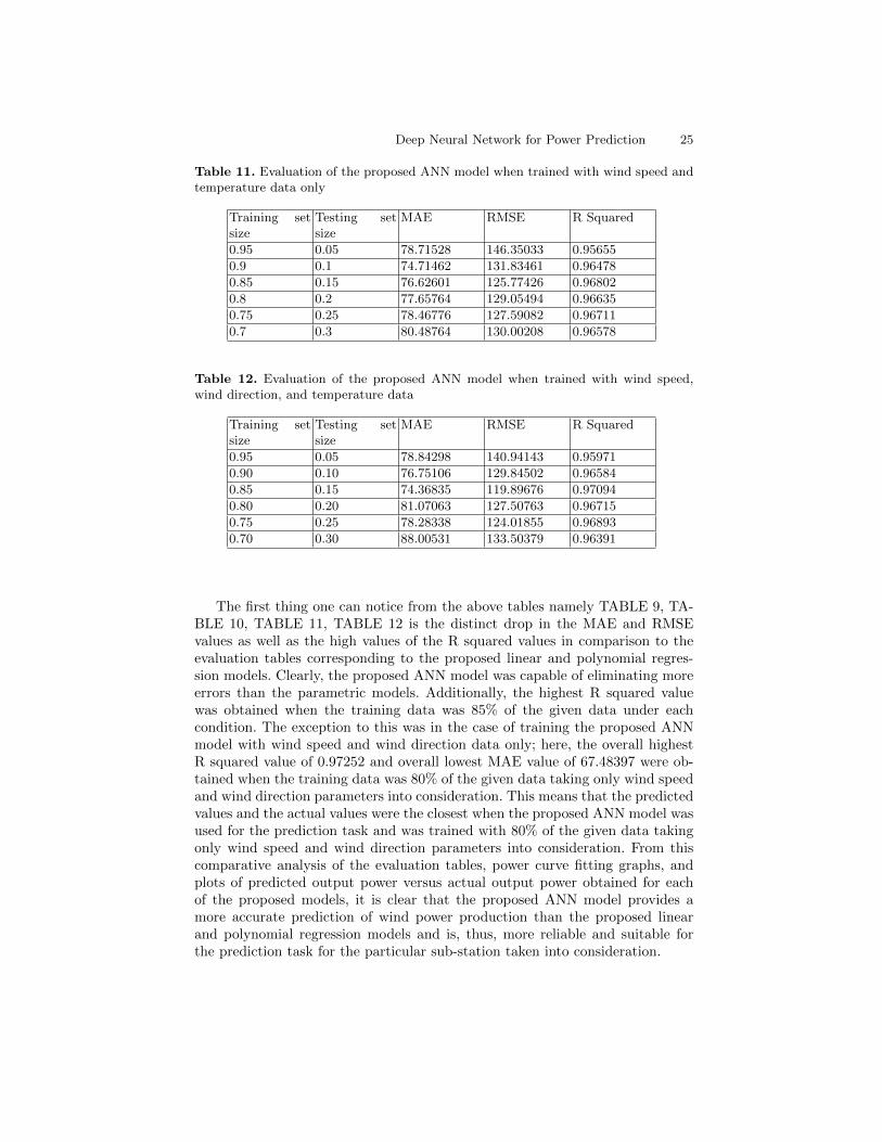
Table 9. Evaluation of the proposed ANN model when trained with wind speed dataonly

Training setsize

Testing setsize

MAE RMSE R Squared

0.95 0.05 77.56814 145.24016 0.95721

0.9 0.1 75.75352 134.63276 0.96327

0.85 0.15 73.47237 125.15547 0.96833

0.8 0.2 75.05013 127.97741 0.96691

0.75 0.25 78.28338 124.01855 0.96892

0.7 0.3 78.77452 129.85588 0.96586

Table 10. Evaluation of the proposed ANN model when trained with wind speed andwind direction data only

Training setsize

Testing setsize

MAE RMSE R Squared

0.95 0.05 73.34284 136.72901 0.96208

0.9 0.1 70.68888 127.45645 0.96708

0.85 0.15 76.62601 125.77426 0.96802

0.8 0.2 67.48397 116.63269 0.97252

0.75 0.25 72.66855 120.72298 0.97056

0.7 0.3 72.15834 121.72978 0.96999


Table 11. Evaluation of the proposed ANN model when trained with wind speed andtemperature data only

Training setsize

Testing setsize

MAE RMSE R Squared

0.95 0.05 78.71528 146.35033 0.95655

0.9 0.1 74.71462 131.83461 0.96478

0.85 0.15 76.62601 125.77426 0.96802

0.8 0.2 77.65764 129.05494 0.96635

0.75 0.25 78.46776 127.59082 0.96711

0.7 0.3 80.48764 130.00208 0.96578

Table 12. Evaluation of the proposed ANN model when trained with wind speed,wind direction, and temperature data

Training setsize

Testing setsize

MAE RMSE R Squared

0.95 0.05 78.84298 140.94143 0.95971

0.90 0.10 76.75106 129.84502 0.96584

0.85 0.15 74.36835 119.89676 0.97094

0.80 0.20 81.07063 127.50763 0.96715

0.75 0.25 78.28338 124.01855 0.96893

0.70 0.30 88.00531 133.50379 0.96391

The first thing one can notice from the above tables namely TABLE 9, TA-BLE 10, TABLE 11, TABLE 12 is the distinct drop in the MAE and RMSEvalues as well as the high values of the R squared values in comparison to theevaluation tables corresponding to the proposed linear and polynomial regres-sion models. Clearly, the proposed ANN model was capable of eliminating moreerrors than the parametric models. Additionally, the highest R squared valuewas obtained when the training data was 85% of the given data under eachcondition. The exception to this was in the case of training the proposed ANNmodel with wind speed and wind direction data only; here, the overall highestR squared value of 0.97252 and overall lowest MAE value of 67.48397 were ob-tained when the training data was 80% of the given data taking only wind speedand wind direction parameters into consideration. This means that the predictedvalues and the actual values were the closest when the proposed ANN model wasused for the prediction task and was trained with 80% of the given data takingonly wind speed and wind direction parameters into consideration. From thiscomparative analysis of the evaluation tables, power curve fitting graphs, andplots of predicted output power versus actual output power obtained for eachof the proposed models, it is clear that the proposed ANN model provides amore accurate prediction of wind power production than the proposed linearand polynomial regression models and is, thus, more reliable and suitable forthe prediction task for the particular sub-station taken into consideration.

26 Alagappan et al.

7 Conclusion

With the prominence of wind power in the global energy market, it is clear thataccurate prediction models are crucial. This is becoming a conspicuous point ofresearch as an important component in operating power systems to maintaintheir reliability. This paper has presented an outline of the different modelsthat have been attempted for power prediction to showcase the diversity inapproaches, and proposed parametric and non-parametric models for performingthe same task. While there are various methods to approach the prediction task,the performance of each model depends upon the particular data set with whichit should operate. Further, it must be noted that short-term models such as theones explored in this paper cannot be directly applied to another site. Theymust be modified by a domain expert in order to take site-specific influencingfactors into consideration. By utilizing modelling methods based on the conceptof the power curve, the prediction of wind power production has been madeconvenient. For the data set provided, the proposed ANN model was best-suitedto predict wind power production, as it gives the best R squared values and theleast RMSE and MAE values. To our knowledge, there are several institutionsassociated with wind energy production and utilization which use polynomialregression - a model that performed second-best with the given data, as canbe seen in this article. This is likely because ANNs take a long time to processlarger and larger data sets,whereas polynomial models are simpler to debug.

8 Declaration of Competing Interest

The authors declare that they have no known competing financial interests orpersonal relationships that could have appeared to influence the work reportedin this paper.

References

1. N. Zouros, G.C. Contaxis, J. Kabouris, ”Decision support tool to evaluate alter-native policies regulating wind integration into autonomous energy systems,” inEnergy Policy, Volume 33, Issue 12, 2005, pp. 1541-1555.

2. R. Abhinav, N.M. Pindoriya, J. Wu, C. Long, ”Short-term wind power forecast-ing using wavelet-based neural network”, in Energy Procedia, Volume 142, 2017,pp. 455-460R. Abhinav, N.M. Pindoriya, J. Wu, C. Long, ”Short-term wind powerforecasting using wavelet-based neural network,” in Energy Procedia, Volume 142,2017, pp. 455-460

3. P.K. Chaurasiya, V. Warudkar, S. Ahmed, ”Wind energy development and policyin India: A review,” in Energy Strategy Reviews, Volume 24, 2019, pp. 342-357

4. W-Y.Chang,”A Literature Review of Wind Forecasting Methods,”in Journal ofPower and Energy Engineering, 02, 2014, pp. 161-168

5. Y.K.Wu and J.S.Hon,”A Literature Review of Wind Forecasting Technology in theWorld,” in Proceedings of IEEE Conference on Power Tech, Lausanne, 1-5 July2007, pp. 504-509


6. M. Lange and H.P. Waldl, ”Assessing the uncertainty of wind power predictionswith regard to specific weather situations,” in Proceedings of the European WindEnergy Conference, Copenhagen, Denmark, June 2001, pp.695-698

7. A. Basu and A. Halder, ”Importance of Numerical Weather Prediction in VariableRenewable Energy Forecast,” 2017

8. A.M. Foley, P.G. Leahy, A. Marvuglia, E.J. McKeogh, ”Current methods and ad-vances in forecasting of wind power generation,” in Renewable Energy, Volume 37,Issue 1, 2012, pp. 1-8

9. J.L. Torres, A. Garcıa, M. De Blas, A. De Francisco, ”Forecast of hourly averagewind speed with ARMA models in Navarre,” in Solar Energy, Volume 79, Issue 1,2005, pp. 65-77

10. R.G.Kavasseri and K.Seetharaman , ”Day-ahead wind speed forecasting using f-ARIMA models,” in Renewable Energy, 34, issue 5, pp. 1388-1393

11. C. Lei and L. Ran, ”Short-term wind speed forecasting model for wind farm basedon wavelet decomposition,” in 2008 Third International Conference on Electric Util-ity Deregulation and Restructuring and Power Technologies, Nanjing, 2008, pp.2525-2529

12. M. A. T. Lira, M. D. S. Emerson, M. B. A. Jose and V. O. V. Gielson, ”Estimationof wind resources in the coast of Ceara, Brazil, using the linear regression theory,”in Renewable and Sustainable Energy Reviews, vol. 39, 2012, pp. 509-529

13. I. E. Kafazi, R. Bannari, O. Aboutafail, A. Abouabdellah, M. Josep, ”EnergyProduction : A Comparison of Forecasting Methods using the Polynomial CurveFitting and Linear Regression,” in Proceedings of the 2017 International Renewableand Sustainable Energy Conference, IRSEC 2017, IEEE Press, 2017 pp. 1-5

14. G. Li and J. Shi, ”On Comparing Three Artificial Nneural Networks for WindSpeed Forecasting,” in Applied Energy, 87, 2010, pp. 2313-2320

15. R. L. Welch, S. M. Ruffing and G. K. Venayagamoorthy, ”Comparison of feed-forward and feedback neural network architectures for short term wind speed pre-diction,” in 2009 International Joint Conference on Neural Networks, Atlanta, GA,2009, pp. 3335-3340

16. R. Jursa and K. Rohrig, ”Short-term wind power forecasting using evolutionaryalgorithms for the automated specification of artificial intelligence models,” in In-ternational Journal of Forecasting, 24, issue 4, 2008, pp. 694-709

17. M. Negnevitsky and C. Potter, ”Innovative short-term wind generation predic-tion techniques (Panel Paper),” in Proceedings of the IEEE/PES General Meeting,Montreal, Canada, 2006, pp. 18–22

18. R. Wadhvani, S. Shukla, M. Gyanchandani and A. Rasool, ”Analysis of statisticaltechniques to estimate wind turbine power generation,” in International Journal ofComputer Science and Network Security (IJCSNS), 17(2), p.247

19. A.Kusiak, H.Zheng and Z.Song,” Models for monitoring wind farm power,” inRenewable Energy, 34(3), 2009, pp.583-590

20. V.Sohoni, S.Gupta and R.Nema, ”A Critical Review on Wind Turbine Power CurveModelling Techniques and Their Applications in Wind Based Energy Systems,” inJournal of Energy, 2016, pp. 1-18

21. F. Pelletier, C. Masson and A. Tahan, ”Wind turbine power curve modelling usingartificial neural network,” in Renewable Energy, 89, 2015, pp. 207-214

22. H.X. Yang, L. Lu and J. Byrnett, ”Weather data and probability analysis of hybridphotovoltaic wind power generation system in Hong Kong,” in Renewable Energy,28, 2003, pp. 1813-1824

ssn college of engineering, kalavakkam, chennai arxiv:2108

Documents