ssw15 (1)
DESCRIPTION
Math workingsTRANSCRIPT
Global weak solutions in a PDE-ODE system modeling multiscale
cancer cell invasion
Christian Stinner1∗ Christina Surulescu1#
Michael Winkler2‡
1 Technische Universitat Kaiserslautern, Felix-Klein-Zentrum fur Mathematik,
Paul-Ehrlich-Str. 31, 67663 Kaiserslautern, Germany2 Institut fur Mathematik, Universitat Paderborn, 33098 Paderborn, Germany
Abstract
We prove the global existence, along with some basic boundedness properties, of weak solutionsto a PDE-ODE system modeling the multiscale invasion of tumor cells through the surroundingtissue matrix. The model has been proposed in [22] and accounts on the macroscopic level for theevolution of cell and tissue densities, along with the concentration of a chemoattractant, while onthe subcellular level it involves the binding of integrins to soluble and insoluble components of theperitumoral region. The connection between the two scales is realized with the aid of a contractiv-ity function characterizing the ability of the tumor cells to adapt their motility behavior to theirsubcellular dynamics.
The resulting system, consisting of three partial and three ordinary differential equations includinga temporal delay, in particular involves chemotactic and haptotactic cross-diffusion. In order toovercome technical obstacles stemming from the corresponding highest-order interaction terms, webase our analysis on a certain functional, inter alia involving the cell and tissue densities in thediffusion and haptotaxis terms respectively, which is shown to enjoy a quasi-dissipative property.This will be used as a starting point for the derivation of a series of integral estimates finally al-lowing for the construction of a generalized solution as the limit of solutions to suitably regularizedproblems.
Key words: chemotaxis; haptotaxis; asymptotic behavior; multiscale model; delay.
AMS Classification: 35Q92, 92C17, 35K57, 35B40.
∗[email protected]#[email protected]‡[email protected]
1
1 Introduction
The model. The migration of cancer cells from the original tumor toward blood vessels and thesubsequent transport to distal sites eventually leading to metastasis establishment is influenced bya plethora of biochemical processes [8]. These take place at several scales, ranging from the level ofsubcellular events and up to the macroscopic behavior of tissue and cell populations. Thereby, thetime scales spread from seconds (or less) for the processes inside cells or on their surface, up to monthsfor the doubling times of tumors or for the time it takes to develop clinically detectable secondarytumors.
Chemotaxis and haptotaxis are two of the main mechanisms conditioning cancer cell motility. Theformer terms the directed cell motion in response to concentration gradients of some chemoattrac-tant/chemorepellent. The latter refers to changes in the orientation and speed of the cell accordingto interactions (mainly adhesion) with the fibers of the extracellular matrix (ECM): The cells will mi-grate from a region of low concentration of relevant adhesive molecules towards a region with a higherconcentration. Mathematical models set up on this macrolevel and involving at least one of these twomechanisms have been proposed and analyzed in literature, see e.g., [2, 34] and the references therein.
The macroscopic features mentioned above are, however, influenced by the internal state of cells, henceby microscopic processes, e.g., receptor binding to chemoattractant or adhesion molecules initiatingintracellular signaling pathways, which in turn lead to restructuring of the cytoskeleton, polarization,production of matrix degrading enzymes (MDEs), proliferation, etc. [7, 13, 14]. Including this mi-crolevel dynamics into the mathematical model leads to a multiscale setting coupling a system ofpartial differential equations (PDEs) for the quantities on the macroscale with ordinary differentialequations (ODEs) modeling the subcellular events. These continuum micro-macro models explicitlyaccounting for subcellular events are rather new, especially in the context of cancer cell migration.Other (mainly individual based) multiscale models connecting the macrolevel with the subcellularand/or cellular scale have been proposed e.g., by Macklin et al. [19] for vascular tumor growth also in-volving mechanic effects or by Ramis-Conde et al. [27, 28], where an individual force-based approachis considered, focusing on the influence of intra- and intercellular dynamics on the cell movement.Hybrid models using cellular automata or agent-based approaches (see e.g., [9, 39, 44]) provide anatural framework for coupling individual events with macrolevel features, thereby allowing for a highlevel of detail. However, when the number of cells greatly increases to biologically realistic valuesthis approach can become very expensive or even intractable from a computational point of view. Incontrast, continuum models describe the evolution of population-averaged phenomena and are moreefficient from a numerical point of view. In this framework Webb et al. [40] studied a populationbased micro-macro model coupling the tumor cell and ECM densities with concentrations of MMP(matrix metalloproteinases) and protons, the latter both in their intracellular and extracellular forms.Mallet & Pettet [20] proposed a model for the integrin-mediated haptotactic migration, which assignsparticular attention to the role played by cell surface receptors in the adhesion to ECM.
All previously mentioned settings focused on the modeling and illustration of the involved dynam-ics by way of numerical simulations, paying less attention to the mathematical well posedness. Thelatter is a nontrivial issue, due to the fact that in the multiscale models different types of equationsare coupled in a highly nonlinear way and the regularity assumptions which can be made are rathermodest, according to biologically motivated requirements. Also, the models are sensitive to changes
2
in the initial data and in the parameter ranges, which in turn are difficult to assess in the absence ofadequate quantitative information. Hence, the solutions to the corresponding systems can exhibit os-cillatory behavior and even blow-up. Such problems are often encountered in chemotaxis systems (seee.g., [3, 5]). Global existence of solutions to systems modeling tumor invasion has been investigatedamong others by Litcanu & Morales-Rodrigo [17] and Tao [30] (accounting for haptotaxis only) and byTao et al. [29, 31, 32, 34] (chemotaxis and haptotaxis jointly influencing the motion). The analyzedmodels were set on the macroscale and described the evolution of tumor cells in interaction with thesurrounding tissue and MDEs, hence coupling reaction-diffusion and ordinary differential equations intwo or three space dimensions. In the context of multiscale cancer cell migration the well posednessissue was addressed e.g., in [15, 18] (micro-meso-macro models) and in [22, 23] (micro-macro models),respectively. The present work is concerned with this problem, too. Here the subcellular (microlevel)dynamics is represented by the binding of integrins to the respective ligands and this is seen as theonset of all subsequent intracellular signaling and its effects on the cell responses. The coupling withthe macrolevel is realized by way of a contractivity function capturing the effects of subcellular dy-namics on the cell motility and carrying them over into the diffusion and haptotaxis coefficients of thecorresponding terms in the equation describing the evolution of tumor cells. This function satisfiesitself a differential equation involving the concentrations of bound integrins as inputs. As the conver-sion of biochemical signals initiated by integrin binding into motile behavior needs a long sequence ofevents to happen, we allow for a time lag in the contractivity equation, which hence takes the form ofa delay differential equation (DDE). We recall here the micro-macro setting in [22] and refer to thatwork for the modeling details. Upon non-dimensionaliziation, the model proposed there becomes
∂tc = ∇ ·(
κ1+cv∇c
)−∇ ·
(κv
1+v c∇v)−∇ ·
(c
1+cl∇l)
+ µcc(1− c− η1v), x ∈ Ω, t > 0,
∂tv = µvv(1− v)− λcv, x ∈ Ω, t > 0,
∂tl = ∆l − l + cv, x ∈ Ω, t > 0,
∂ty1 = k1(1− y1 − y2)v − k−1y1, x ∈ Ω, t > 0,
∂ty2 = k2(1− y1 − y2)l − k−2y2, x ∈ Ω, t > 0,
∂tκ = −κ+ My1(·,t−τ)1+y2(·,t−τ) , x ∈ Ω, t > 0,
(1.1)
the dependent variables respectively representing the following:
• c(x, t): cancer cell density;
• v(x, t): density of tissue fibers in the ECM;
• l(x, t): concentration of chemoattractant (i.e., proteolytic rests resulting from degradation ofECM fibers by matrix degrading enzymes produced by the tumor cells);
• y1(x, t): concentration of integrins bound to ECM fibers;
• y2(x, t): concentration of integrins bound to proteolytic residuals;
• κ(x, t): contractivity function;
• µc: proliferation rate of tumor cells;
3
• µv: production/re-establishment rate of ECM fibers;
• δ: degradation rate of ECM fibers due to the action of MDEs;
• η1, η2: interaction rates allowing to take crowding into account;
• k−1, k1, k−2, k2: reaction rates in the binding of integrins to insoluble (ECM fibers) and soluble(proteolytic rests) ligands in the peritumoral environment.
Moreover, we abbreviate λ := δ + µvη2.
Mathematical challenges. The goal of the present work is to establish a result on global solv-ability of (1.1) in an adequate framework. From a mathematical point of view, this amounts toappropriately overcome several difficulties inherent to (1.1) and, in particular, the strong couplingstherein. Indeed, as a subsystem the model (1.1) contains a Keller-Segel-type chemotaxis system, theoriginal form of which, that is,
∂tc = ∆c−∇ · (c∇l), x ∈ Ω, t > 0,
∂tl = ∆l − l + c, x ∈ Ω, t > 0,(1.2)
is known to exhibit phenomena of blow-up in finite time when either n ≥ 3 (see [43]) or n = 2 and thetotal mass of cells is supercritical [10, 24]. As compared to (1.2), both the diffusivity D(c, v) := κ
1+cvand the chemotactic sensitivity χ(c, l) := c
1+cl in (1.1) depend nonlinearly on c, v, and l, thus leadingto an even higher complexity of interaction. In [4] it has been shown that in the neighboring casewhen D = D(c) = 1
1+c and χ = χ(c) = c1+c , blow-up in the correspondingly adapted variant of
(1.2) does as well occur at least when n = 3. Anyhow, the logistic-type cell kinetic term in the firstequation in (1.1), is known to have a certain blow-up preventing effect on chemotaxis systems: Whenaccordingly introduced in (1.2), for instance, proliferation terms of the form µcc(1− c) are known toenforce boundedness of solutions when n ≤ 2 (see [25]), and also when n ≥ 3 and µc is suitably large[42]; however, this apparently does not exclude the possibility of explosions when n = 3 and µc issmall.
A second subsystem is obtained upon focusing on the cross-diffusive interaction with v, resulting in avariant of the prototypical haptotaxis system
∂tc = ∆c−∇ · (c∇v), x ∈ Ω, t > 0,
∂tv = f(c, v), x ∈ Ω, t > 0,(1.3)
with given f . Here the lack of diffusibility of v is reflected in the absence of any regularizing effecton v during evolution. Correspondingly, the mathematical literature on (1.3) is comparatively thin,the main contributions on haptotaxis systems concentrating on particular choices of f [6, 38] or onmodified variants involving additional dampening effects such as logistic growth inhibition [21, 17].More recently, certain combined chemotaxis-haptotaxis models with linear cell diffusion and standardcross-diffusive terms as in (1.2) and (1.3), have been investigated, and some results on global existenceand also on asymptotic solution behavior could be gained for various special choices of f in therespective ODE ∂tv = f(c, v, l) [29, 33, 35, 36, 12].
Main results. In the sequel, we shall consider the PDE-ODE system (1.1) in a bounded domain
4
Ω ⊂ Rn, n ≤ 3, with smooth boundary, under no-flux boundary conditions (ν denotes the outernormal to ∂Ω):
κ
1 + cv∂νc−
κv
1 + vc ∂νv = ∂ν l = 0, x ∈ ∂Ω, t > 0, (1.4)
and the initial conditions
c(x, 0) = c0(x), v(x, 0) = v0(x), l(x, 0) = l0(x), κ(x, 0) = κ0(x), x ∈ Ω,
y1(x, t) = y10(x, t), y2(x, t) = y20(x, t), x ∈ Ω, t ∈ [−τ, 0], (1.5)
where we assume that
c0 ∈ C0(Ω), v0 ∈W 1,2(Ω) ∩ C0(Ω), l0 ∈W 1,2(Ω) ∩ C0(Ω), κ0 ∈W 1,4(Ω),
y10 ∈ C0([−τ, 0];W 1,4(Ω)) and y20 ∈ C0([−τ, 0];W 1,4(Ω)) (1.6)
satisfy
c0 ≥ 0, v0 ≥ 0, l0 > 0, κ0 > 0 in Ω as well as
y10 ≥ 0, y20 ≥ 0 and y10 + y20 ≤ 1 in Ω× (−τ, 0). (1.7)
The parameters µc, η1, µv, λ := δ+µvη2, k1, k−1, k2, k−2,M and τ are assumed to be positive through-out.
In this mathematical setting, the main outcome of this paper then establishes the global existenceof solutions in an appropriate generalized sense, along with some basic global qualitative properties.Besides providing accessibility to our mathematical approach described below, such a resort to weaksolutions may be adequate also from a biological point of view: As cell migration is a process featuredby very complex phenomena and influenced by a strongly heterogeneous and rapidly modifying en-vironment, the cell and fiber densities – though existing globally in time – should be allowed to beless regular and the conditions for their existence to be less restrictive than, for instance, required inframeworks of classical solutions.
In its precise formulation, our main result reads as follows.
Theorem 1.1 Let n ≤ 3 and Ω ⊂ Rn be a bounded domain with smooth boundary, and suppose thatc0, v0, l0, y10, y20 and κ0 comply with (1.6) and (1.7). Then (1.1), (1.4), (1.5) possesses at least oneglobal weak solution in the sense specified in Definition 5.1 below. Moreover, this solution has thefollowing global boundedness properties: There exists C > 0 such that
∫Ωc(·, t) ≤ C and
∫ t+1
t
∫Ωc2 ≤ C for all t > 0,
v ≤ C in Ω× (0,∞),
‖l(·, t)‖W 1,2(Ω) ≤ C and
∫ t+1
t‖l(·, s)‖2W 2,2(Ω)ds ≤ C for all t > 0,
y1 ≤ C in Ω× (0,∞),
y2 ≤ C in Ω× (0,∞) and
κ ≤ C in Ω× (0,∞).
(1.8)
5
Main ideas underlying our approach. A cornerstone of our analysis will consist of identifyinga certain quasi-dissipative property of the functional
E :=
∫Ωc ln c+
1
2λ
∫Ω
κ|∇v|2
1 + v.
Indeed, we shall see in Lemma 4.1 below that a certain regularized variant thereof satisfies an inequalityof the form
d
dtE +D ≤ F (t)E +H(t− τ), t > 0, (1.9)
with some nonnegative F ∈ L1loc[0,∞)), a function H ∈ L1
loc([0,∞)) allowing for the estimate
H(t− τ) ≤ CE(t− τ) for all t > τ
with some C > 0, and with the dissipation rate given by
D :=1
2
∫Ω
κ
1 + cv
|∇c|2
c+
∫Ωκc|∇v|2
(1 + v)2+µc2
∫Ωc2 ln(2 + c)
(cf. (4.31)). In particular, this will imply an integral estimate of the form
E(t) ≤ C(T ) + C(T )
∫ t
0E(σ)dσ for all t > 0
with suitably large C > 0 (see (4.36)), whereupon the Grønwall lemma will provide bounds for
supt∈(0,T ) E(t) and∫ T
0 D(t)dt for any fixed T > 0. These in turn will form the fundament for ourderivation of appropriate compactness properties of solutions to the regularized problems (2.1) below(see Section 5.1), and thereby finally allow for the construction of weak solutions as limits of globalsmooth solutions to these approximate problems in Section 5.2.Finally, in Section 6 we will comment on some possible model extensions.
2 A family of approximate problems
In order to construct a solution of (1.1), (1.4), (1.5), let us first consider the regularized problems
∂tcε = ε∆cε +∇ ·(
κε1+cεvε
∇cε)−∇ ·
(κεvε1+vε
cε∇vε)−∇ ·
(cε
1+cεlε∇lε)
+µccε(1− cε − η1vε)− εcθε, x ∈ Ω, t > 0,
∂tvε = ε∆vε + µvvε(1− vε)− λcεvε, x ∈ Ω, t > 0,
∂tlε = ∆lε − lε + cεvε, x ∈ Ω, t > 0,
∂ty1ε = k1(1− y1ε − y2ε)vε − k−1y1ε, x ∈ Ω, t > 0,
∂ty2ε = k2(1− y1ε − y2ε)lε − k−2y2ε, x ∈ Ω, t > 0,
∂tκε = −κε + My1ε(·,t−τ)1+y2ε(·,t−τ) , x ∈ Ω, t > 0,
∂νcε = ∂νvε = ∂ν lε = 0, x ∈ ∂Ω, t > 0,
cε(x, 0) = c0ε(x), vε(x, 0) = v0ε(x), lε(x, 0) = l0ε(x), κε(x, 0) = κ0ε(x), x ∈ Ω,
y1ε(x, t) = y10ε(x, t), y2ε(x, t) = y20ε(x, t), x ∈ Ω, t ∈ [−τ, 0]
(2.1)
6
for ε ∈ (0, 1), where θ > max2, n is a fixed parameter and (c0ε)ε∈(0,1), (v0ε)ε∈(0,1), (l0ε)ε∈(0,1),(κ0ε)ε∈(0,1), (y10ε)ε∈(0,1) and (y20ε)ε∈(0,1) are families of functions
c0ε ∈ C3(Ω), v0ε ∈ C3(Ω), l0ε ∈ C3(Ω), κ0ε ∈ C3(Ω),
y10ε ∈ C3(Ω× [−τ, 0]) and y20ε ∈ C3(Ω× [−τ, 0]) (2.2)
which are all positive and satisfy
∂νc0ε = ∂νv0ε = ∂ν l0ε = 0 on ∂Ω and y10ε + y20ε < 1 in Ω× [−τ, 0] (2.3)
for all ε ∈ (0, 1) as well as
c0ε → c0 in C0(Ω),
v0ε → v0 in W 1,2(Ω) ∩ C0(Ω),
l0ε → l0 in W 1,2(Ω) ∩ C0(Ω),
κ0ε → κ0 in W 1,4(Ω),
y10ε → y10 in C0([−τ, 0];W 1,4(Ω)) and
y20ε → y20 in C0([−τ, 0];W 1,4(Ω))
(2.4)
as ε 0.We shall see in Lemma 3.11 below that each of these problems possesses a global classical solution.
3 Global existence and basic estimates for the regularized problems
3.1 Local existence
Let us first assert the local existence of smooth solutions to (2.1).
Lemma 3.1 For any ε ∈ (0, 1) there exist Tε ∈ (0,∞] and a collection of positive functions cε, vε, lε,y1ε, y2ε and κε, all belonging to C2,1(Ω× [0, Tε)), which solve (2.1) in the classical sense in Ω× (0, Tε)and have the additional property that
if Tε <∞ then lim suptTε
‖cε(·, t)‖C2+β(Ω) + ‖vε(·, t)‖C2+β(Ω) + ‖lε(·, t)‖C2+β(Ω)
+‖y1ε(·, t)‖C2+β(Ω) + ‖y2ε(·, t)‖C2+β(Ω) + ‖κε(·, t)‖C2+β(Ω)
=∞ for all β ∈ (0, 1). (3.1)
Proof. We fix ε ∈ (0, 1) and β ∈ (0, 1) and define
A := ‖c0ε‖C2+β(Ω) + ‖v0ε‖C2+β(Ω) + ‖l0ε‖C2+β(Ω) + ‖y10ε‖C2+β,1+
β2 (Ω×[−τ,0])
+‖y20ε‖C2+β,1+
β2 (Ω×[−τ,0])
+ ‖κ0ε‖C2+β(Ω).
Furthermore, we define c0εt(x) to be the right-hand side of the first equation of (2.1) evaluated at(x, t) = (x, 0). This means that
B := ‖c0ε‖Cβ(Ω) + ‖c0εt‖C0(Ω) ≤ C1(A) <∞ (3.2)
7
is satisfied with a constant C1(A) depending on A. Next, we fix T ∈ (0, 1] and set
X :=
cε ∈ Cβ,
β2 (Ω× [0, T ]) : cε ≥ 0, ‖cε‖
Cβ,β2 (Ω×[0,T ])
≤ B + 1
.
Given a fixed cε ∈ X, by [16, Theorems V.7.4 and IV.5.3], (2.2), (2.3), v0ε > 0 and the (strong)parabolic maximum principle, there exists a solution vε to the second equation of (2.1) with thehomogeneous Neumann boundary condition and initial data v0ε such that 0 < vε ≤ max1, ‖v0ε‖C0(Ω)in Ω× [0, T ] and
‖vε‖C2+β1,1+
β12 (Ω×[0,T ])
≤ C2(A) (3.3)
with some β1 ∈ (0, β] and some constant C2(A) > 0 which in view of (3.2) may depend on A. Then,using similar arguments we obtain the existence of a positive solution lε to the third equation of (2.1)with the homogeneous Neumann boundary condition and initial data l0ε satisfying
‖lε‖C2+β2,1+
β22 (Ω×[0,T ])
≤ C3(A) (3.4)
with some constant C3(A) > 0 and some β2 ∈ (0, β1]. Next, as the fourth and fifth equations of (2.1)form a linear system of ODEs for (y1ε, y2ε), by using (3.3), (3.4) and (2.2) we deduce that there exists
a solution to this system with initial data (y10ε, y20ε) which fulfills yiε ∈ C2+β2,1+β22 (Ω× [0, T ]) as well
as
‖yiε‖Cβ2,
β22 (Ω×[−τ,T−τ ])
+
∥∥∥∥∂yiε∂xj
∥∥∥∥Cβ2,
β22 (Ω×[−τ,T−τ ])
+
∥∥∥∥ ∂2yiε∂xj∂xk
∥∥∥∥Cβ2,
β22 (Ω×[−τ,T−τ ])
≤ C4(A) (3.5)
for all i ∈ 1, 2 and j, k ∈ 1, . . . , n with some C4(A) > 0. Since moreover Y with Y := (y1, y2) ∈(0, 1)2 : y1 + y2 < 1 is a positive invariant set for this system of ODEs, (2.3), the positivity of theinitial data and applications of the comparison principle to y1ε, y2ε and y1ε + y2ε, respectively, implythat (y1ε, y2ε) cannot reach the boundary of Y in finite time and therefore remains inside the positivecone in R2.Next, in view of (2.2), (3.5) and the positivity of κ0ε, there is a solution κε to the linear ODE formedby the sixth equation of (2.1) with initial data κ0ε which is positive by the comparison principle andsatisfies
‖κε‖C2+β2,1+
β22 (Ω×[0,T ])
≤ C5(A) (3.6)
with some constant C5(A) depending on A. Taking now these functions vε, lε and κε and using [16,Theorems V.7.4 and IV.5.3], (2.2), (2.3), (3.3), (3.4), (3.6) and the positivity of c0ε, we obtain a
solution cε ∈ C2+β3,1+β32 (Ω × [0, T ]) to the first equation of (2.1) with the homogeneous Neumann
boundary condition and initial data c0ε for some β3 ∈ (0, β2] which is positive by the strong maximumprinciple and fulfills
‖cε‖C2+β3,1+
β32 (Ω×[0,T ])
≤ C6(A) (3.7)
with some constant C6(A) depending on A. In particular, we have
‖∂tcε‖Cβ3,
β32 (Ω×[0,T ])
≤ C6(A) (3.8)
8
and the regularity of cε implies that c0εt(x) = ∂tcε(x, 0) for x ∈ Ω with the definition of c0εt given inthe beginning of this proof. Therefore, (3.2) and (3.8) yield the existence of T0 ∈ (0, 1] just dependingon A such that
‖cε‖Cβ,
β2 (Ω×[0,T1])
≤ B + 1
for T1 := minT0, T, where we have used the fact that ‖f‖Cβ2 ([0,T1])
≤ ‖f‖C1([0,T1]) holds for f ∈
C1([0, T1]) due to T1 ≤ 1. Hence, setting now T := T0, we have cε ∈ X so that the map F : X → X,F (cε) := cε for cε ∈ X, is well-defined and compact in view of (3.7). Since X is a closed, bounded and
convex subset of Cβ,β2 (Ω× [0, T ]), F has a fixed point cε by Schauder’s fixed point theorem. Starting
with this cε, the above reasoning gives the existence of a classical solution to (2.1) in Ω× [0, T0] suchthat all components are positive and belong to C2,1(Ω× [0, T0]).Finally, since T0 just depends on A, the solution to (2.1) can be extended up to some T2 > Tε if allcomponents are uniformly bounded in C2+β(Ω) for t ∈ (0, Tε) (because in case of Tε > τ > 0 then y1ε
and y2ε are uniformly bounded in C2+β,1+β2 (Ω × [0, T3 − τ ]) for some T3 > Tε which in view of (3.5)
is sufficient to extend the solution up to some T2 ∈ (Tε, T3]). Hence, (3.1) is proved as β ∈ (0, 1) wasarbitrary.
3.2 Some elementary ε-independent estimates
Some basic but important properties of cε and vε are summarized in the next two lemmata.
Lemma 3.2 The solution of (2.1) satisfies∫Ωcε(·, t) ≤ m := max
supε∈(0,1)
∫Ωc0ε , |Ω|
for all t ∈ (0, Tε) (3.9)
and ∫ t+1
t
∫Ωc2ε ≤
µc + 1
µc·m for all t ∈ (0, Tε − 1) (3.10)
as well as
ε
∫ t+1
t
∫Ωcθε ≤ (µc + 1)m for all t ∈ (0, Tε − 1). (3.11)
Proof. A spatial integration of the first equation in (2.1) yields
d
dt
∫Ωcε = µc
∫Ωcε(1− cε − η1vε)− ε
∫Ωcθε
≤ µc
∫Ωcε − µc
∫Ωc2ε − ε
∫Ωcθε for all t ∈ (0, Tε), (3.12)
so that since∫
Ω c2ε ≥ 1
|Ω|(∫
Ω cε)2 by the Cauchy-Schwarz inequality, an ODE comparison shows (3.9).
Thereafter, (3.10) and (3.11) easily result upon an integration of (3.12) over (t, t+ 1).
Lemma 3.3 For each ε ∈ (0, 1), we have
vε(x, t) ≤ Kv := max
supε∈(0,1)
‖v0ε‖L∞(Ω) , 1
for all x ∈ Ω and t ∈ (0, Tε).
9
Proof. This is a straightforward consequence of the parabolic maximum principle applied to thesecond equation in (2.1).
Our next goal is to derive some first regularity properties of lε. For the argument in the respectiveLemma 3.5 below we prepare the following auxiliary statement.
Lemma 3.4 Let T > 0, and suppose that z is a nonnegative absolutely continuous function on [0, T )satisfying
z′(t) + az(t) ≤ f(t) for a.e. t ∈ (0, T ) (3.13)
with some a > 0 and a nonnegative function f ∈ L1loc([0, T )) for which there exists b > 0 such that∫ t+1
tf(s)ds ≤ b for all t ∈ [0, T − 1).
Then
z(t) ≤ max
z(0) + b ,
b
a+ 2b
for all t ∈ (0, T ). (3.14)
Proof. In view of the nonnegativity of z and f , an integration of (3.13) shows that
z(t) ≤ z(t0) +
∫ t
t0
f(s) ds ≤ z(t0) + b for all t0 ∈ [0, T ) and all t ∈ [t0, t0 + 1] ∩ [0, T ). (3.15)
Next, setting γ := maxz(0), ba + b and i0 := maxi ∈ N0 : i < T, we claim that
z(i) ≤ γ for all i ∈ 0, . . . , i0. (3.16)
Obviously, z(0) ≤ γ is fulfilled. Assuming that z(i) ≤ γ for some i ∈ 0, . . . , i0 − 1, we either havez(t) ≥ b
a for all t ∈ [i, i+ 1], so that an integration of (3.13) yields
z(i+ 1) ≤ z(i)− a · ba
+ b = z(i) ≤ γ,
or z(t) < ba for some t ∈ [i, i+ 1], which means z(i+ 1) ≤ z(t) + b ≤ γ by (3.15). Hence, (3.16) holds
by induction. Finally, a combination of (3.16) and (3.15) with t0 = i for i ∈ 0, . . . , i0 proves (3.14).
We can now collect a list of estimates for lε.
Lemma 3.5 There exists C > 0 such that for all ε ∈ (0, 1),
‖lε(·, t)‖W 1,2(Ω) ≤ C for all t ∈ (0, Tε) (3.17)
and ∫ t+1
t‖lε(·, t)‖2W 2,2(Ω)ds ≤ C for all t ∈ (0, Tε − 1) (3.18)
as well as ∫ t+1
t
∫Ω
(∂tlε)2 ≤ C for all t ∈ (0, Tε − 1). (3.19)
Moreover,
lε(x, t) ≥
infε∈(0,1)
infx∈Ω
l0ε(x)· e−t for all x ∈ Ω and t ∈ (0, Tε). (3.20)
10
Proof. We first integrate the third equation in (2.1) and use Lemma 3.2 and Lemma 3.3 to seethat
d
dt
∫Ωlε = −
∫Ωlε +
∫Ωcεvε ≤ −
∫Ωlε +mKv for all t ∈ (0, Tε),
which by an ODE comparison implies that∫Ωlε(·, t) ≤ C1 := max
supε∈(0,1)
∫Ωl0ε , mKv
for all t ∈ (0, Tε). (3.21)
We next test the PDE for lε by −∆lε and use Young’s inequality to find, again relying on Lemma 3.3,that
1
2
d
dt
∫Ω|∇lε|2 +
∫Ω|∆lε|2 +
∫Ω|∇lε|2 = −
∫Ωcεvε∆lε
≤ 1
2
∫Ω|∆lε|2 +
K2v
2
∫Ωc2ε for all t ∈ (0, Tε). (3.22)
In particular, this shows that zε(t) :=∫
Ω |∇lε(·, t)|2, t ∈ [0, Tε), satisfies
z′ε(t) + 2zε(t) ≤ fε(t) := K2v
∫Ωc2ε(·, t) for all t ∈ (0, Tε),
where from Lemma 3.2 we know that∫ t+1
tfε(s)ds ≤ C1 := K2
v ·µc + 1
µc·m for all t ∈ [0, Tε − 1). (3.23)
Hence, Lemma 3.4 applies to warrant that∫Ω|∇lε(·, t)|2 ≤ max
supε∈(0,1)
∫Ω|∇l0ε|2 + C1 ,
5
2C1
for all t ∈ (0, Tε), (3.24)
which combined with (3.21) and (2.4) yields (3.17).Now (3.18) easily follows from this and, again, (3.23) and (3.24) upon a time integration in (3.22). Theinequality (3.19) is then immediate from (3.18) and (3.10). Finally, (3.20) results upon an applicationof the parabolic comparison principle.
For the last three components in (2.1) we can derive some pointwise bounds by elementary ODEcomparison arguments in the following two lemmata.
Lemma 3.6 Given any ε ∈ (0, 1), we have the pointwise estimate
y1ε(x, t) + y2ε(x, t) ≤ Ky := 1 for all x ∈ Ω and t ∈ (−τ, Tε). (3.25)
Proof. It is clear by (2.3) that the claimed inequality holds for all (x, t) ∈ Ω × (−τ, 0]. As forpositive t, we add the respective equations in (2.1) to obtain
∂t(y1ε + y2ε) =
1− (y1ε + y2ε)·k1vε + k2lε
− k−1y1ε − k−2y2ε
≤
1− (y1ε + y2ε)·k1vε + k2lε
in Ω× (0, Tε),
which immediately implies (3.25) by an ODE comparison.
11
Lemma 3.7 Let Ky be as given by Lemma 3.6. Then for all ε ∈ (0, 1), the function κε has theproperties
κε(x, t) ≤ Kκ := max
supε∈(0,1)
‖κ0ε‖L∞(Ω) , MKy
for all x ∈ Ω and t ∈ (0, Tε) (3.26)
andκε(x, t) ≥
inf
ε∈(0,1)infx∈Ω
κ0ε(x)· e−t for all x ∈ Ω and t ∈ (0, Tε) (3.27)
as well as|∂tκε(x, t)| ≤ Kκ for all x ∈ Ω and t ∈ (0, Tε). (3.28)
Proof. Since 0 ≤ yiε(x, t − τ) ≤ Ky for all (x, t) ∈ Ω × (0, Tε) and i ∈ 1, 2 by Lemma 3.6, κεsatisfies −κε ≤ ∂tκε ≤ −κε +MKy ≤MKy in Ω× (0, Tε). By integration, this first implies (3.26) and(3.27) and then proves (3.28) by using (3.26).
3.3 Global existence in the approximate problems
We next aim at proving that all problems (2.1) are in fact globally solvable. To this end, in viewof (3.1) it is sufficient to derive, given any fixed ε ∈ (0, 1), bounds for all solution components withrespect to the norm in C2+β(Ω) with some β > 0.We begin by performing a standard testing procedure to the first equation in (2.1).
Lemma 3.8 Let ε ∈ (0, 1) and p > 1. Then there exists C(ε, p) > 0 such that
1
p
d
dt
∫Ωcpε +
(p− 1)ε
2
∫Ωcp−2ε |∇cε|2 ≤ C(ε, p)
∫Ωcpε|∇vε|2 + C(ε, p)
∫Ωcpε|∇lε|2 + µc
∫Ωcpε (3.29)
for all t ∈ (0, Tε).
Proof. We multiply the first equation in (2.1) by cp−1ε to see upon integrating by parts and
dropping nonnegative terms that
1
p
d
dt
∫Ωcpε + (p− 1)ε
∫Ωcp−2ε |∇cε|2 ≤ (p− 1)
∫Ω
κεvε1 + vε
cp−1ε ∇cε · ∇vε
+(p− 1)
∫Ω
1
1 + cεlεcp−1ε ∇cε · ∇lε
+µc
∫Ωcpε for all t ∈ (0, Tε). (3.30)
Here, recalling Lemma 3.7 and Lemma 3.3 and using Young’s inequality we see that
(p− 1)
∫Ω
κεvε1 + vε
cp−1ε ∇cε · ∇vε ≤
(p− 1)ε
4
∫Ωcp−2ε |∇cε|2 +
p− 1
εK2κK
2v
∫Ωcpε|∇vε|2,
and similarly we obtain
(p− 1)
∫Ω
1
1 + cεlεcp−1ε ∇cε · ∇lε ≤
(p− 1)ε
4
∫Ωcp−2ε |∇cε|2 +
p− 1
ε
∫Ωcpε|∇lε|2
12
for all t ∈ (0, Tε). Hence, (3.29) results from (3.30).
The next lemma will enable us to estimate the first two integrals on the right of (3.29) suitably. Itsproof is the only place where we need our assumption that the exponent in the artificial absorptiveterm in the first equation of (2.1) satisfies θ > maxn, 2.
Lemma 3.9 Let T > 0. Then for each ε ∈ (0, 1) one can find C(ε, T ) > 0 such that∫ Tε
0
(‖∇vε(·, t)‖2L∞(Ω) + ‖∇lε(·, t)‖2L∞(Ω)
)dt ≤ C(ε, T ) (3.31)
holds for Tε = minT, Tε.
Proof. From Lemma 3.2 we know that∫ Tε
0
∫Ωcθε ≤
(µc + 1)m(T + 1)
ε, (3.32)
so that since vε ≤ Kv by Lemma 3.3, fε := ∂tvε − ε∆vε ≡ µvvε(1 − vε) − λcεvε is bounded inLθ(Ω× (0, Tε)). Therefore, known results on maximal Sobolev regularity in parabolic equations ([11])assert that ∫ Tε
0‖vε(·, t)‖θW 2,θ(Ω)dt ≤ C1(ε, T ) (3.33)
with some C1(ε, T ) > 0. Similarly, also gε := ∂tlε−∆lε + lε ≡ cεvε belongs to Lθ(Ω× (0, Tε)), whenceapplying the same regularity result to the third equation in (2.1) yields C2(ε, T ) > 0 fulfilling∫ Tε
0‖lε(·, t)‖θW 2,θ(Ω)dt ≤ C2(ε, T ). (3.34)
As θ > 2 and W 2,θ(Ω) → W 1,∞(Ω) thanks to the additional assumption θ > n, (3.33) and (3.34)imply (3.31).
We can thereby estimate cε in L∞((0, T );Lp(Ω)) for any p ∈ (1,∞) and each finite T ≤ Tε.
Lemma 3.10 Let p > 1 and T > 0. Then for all ε ∈ (0, 1) there exists C(ε, p, T ) > 0 such that∫Ωcpε(·, t) ≤ C(ε, p, T ) for all t ∈ (0, Tε). (3.35)
Proof. By Lemma 3.8, we can find C1(ε, p) > 0 such that
d
dt
∫Ωcpε ≤ C1(ε, p) ·
(‖∇vε(·, t)‖2L∞(Ω) + ‖∇lε(·, t)‖2L∞(Ω)
)·∫
Ωcpε + pµc
∫Ωcpε
for all t ∈ (0, Tε), so that an integration yields∫Ωcpε(·, t) ≤
(∫Ωcp0ε
)· exp
C1(ε, p) ·
∫ t
0
(‖∇vε(·, s)‖2L∞(Ω) + ‖∇lε(·, s)‖2L∞(Ω)
)ds+ pµct
for all t ∈ (0, Tε). In view of Lemma 3.9, this proves (3.35).
Now the desired result on global existence in (2.1) can be derived in a straightforward manner.
13
Lemma 3.11 For each ε ∈ (0, 1), the solution of (2.1) from Lemma 3.1 is global in time; that is, wehave Tε =∞.
Proof. Assuming on the contrary that Tε is finite for some ε ∈ (0, 1), from Lemma 3.10 andparabolic regularity theory ([16]) applied to the second and third equation in (2.1) in combinationwith Lemma 3.3 and Lemma 3.7 we would obtain that the coefficient functions
aε(x, t, q) := εq +κε(x, t)
1 + cε(x, t)vε(x, t)q − κε(x, t)vε(x, t)
1 + vε(x, t)cε(x, t)∇vε(x, t)
− cε(x, t)
1 + cε(x, t)lε(x, t)∇lε(x, t), (x, t, q) ∈ Ω× (0, Tε)× Rn,
and
bε(x, t) := µccε(x, t) ·(
1− cε(x, t)− η1vε(x, t))− εcθε(x, t), (x, t) ∈ Ω× (0, Tε),
in
∂tcε = ∇ ·(aε(x, t,∇cε)
)+ bε(x, t), (x, t) ∈ Ω× (0, Tε),
would satisfy
aε(x, t, q)q ≥ε
2|q|2 − ψ0(x, t) for all (x, t, q) ∈ Ω× (0, Tε)× Rn
and
|aε(x, t, q)| ≤ (ε+Kκ)|q|+ ψ1(x, t) for all (x, t, q) ∈ Ω× (0, Tε)× Rn
as well as
|bε(x, t)| ≤ ψ2(x, t) for all (x, t) ∈ Ω× (0, Tε)
with certain functions ψ0, ψ1 and ψ2 all belonging to⋂p>1 L
p(Ω×(0, Tε)). Therefore, parabolic Holderestimates ([26, Theorem 1.3 and Remark 1.4]) would yield β ∈ (0, 1) and C1(ε) > 0 such that
‖cε‖Cβ,
β2 (Ω×[0,Tε])
≤ C1(ε).
According to standard parabolic Schauder estimates ([16]), this in turn would provide bounds for vε
and lε in C2+β,1+β2 (Ω × [0, Tε]), which would directly entail corresponding estimates for y1ε, y2ε and
κε in the latter space. Again by parabolic Schauder theory, this would now imply that also cε lies in
C2+β,1+β2 (Ω× [0, Tε]) and thereby contradict the extensibility criterion (3.1) in Lemma 3.1.
4 An entropy-type functional
The goal of the present section is to establish the following estimate which has its origin in (1.9).
14
Lemma 4.1 Let T > 0. Then there exists C(T ) > 0 such that for any choice of ε ∈ (0, 1) the solutionof (2.1) satisfies
supt∈(0,T )
∫Ωcε ln cε +
∫Ω
κε|∇vε|2
1 + vε
+ε
∫ T
0
∫Ω
|∇cε|2
cε+
∫ T
0
∫Ω
κε1 + cεvε
|∇cε|2
cε
+
∫ T
0
∫Ωκεcε
|∇vε|2
(1 + vε)2+
∫ T
0
∫Ωc2ε ln(2 + cε)
+ε
∫ T
0
∫Ωcθε ln(2 + cε)
≤ C(T ). (4.1)
The proof thereof will be prepared by a series of integral estimates. The first of these, to be given inLemma 4.3, requires itself as a preliminary the following elementary observation.
Lemma 4.2 There exists C > 0 such that
ξ ln ξ − ξ2 ln ξ ≤ −1
2ξ2 ln(2 + ξ) + C for all ξ > 0 (4.2)
and
−ξθ ln ξ ≤ −1
2ξθ ln(2 + ξ) + C for all ξ > 0 and θ > 0. (4.3)
Proof. To see (4.2), we note that φ : [0,∞) → R with φ(0) := 0 and φ(ξ) := ξ ln ξ − ξ2 ln ξ +12ξ
2 ln(2 + ξ), ξ > 0, defines a continuous function which satisfies φ(ξ) → −∞ as ξ → ∞, so thatφ(ξ) < 0 for all ξ > ξ0 with some ξ0 > 0. Thus, (4.2) follows if we pick any C > maxξ∈[0,ξ0] φ(ξ). Averification of (4.3) can be achieved in much the same manner.
We can thereby give some basic information on the time evolution of the first integral on the left of(4.1).
Lemma 4.3 There exists C > 0 such that for any ε ∈ (0, 1) we have
d
dt
∫Ωcε ln cε + ε
∫Ω
|∇cε|2
cε+
1
2
∫Ω
κε1 + cεvε
|∇cε|2
cε+µc2
∫Ωc2ε ln(2 + cε) +
ε
2
∫Ωcθε ln(2 + cε)
≤∫
Ω
κεvε1 + vε
∇cε · ∇vε +1
2
∫Ω
cε(1 + cεvε)
κε(1 + cεlε)2|∇lε|2 + C for all t > 0. (4.4)
Proof. Since cε is positive in Ω × [0,∞) according to the strong maximum principle, we can usethe first equation in (2.1) to compute
d
dt
∫Ωcε ln cε =
∫Ω
ln cε · ∂tcε +
∫Ω∂tcε
= −ε∫
Ω
|∇cε|2
cε−∫
Ω
κε1 + cεvε
|∇cε|2
cε+
∫Ω
κεvε1 + vε
∇cε · ∇vε +
∫Ω
1
1 + cεlε∇cε · ∇lε
+µc
∫Ω
cε ln cε − c2
ε ln cε
− µcη1
∫Ωcε ln cε vε − ε
∫Ωcθε ln cε
+µc
∫Ωcε(1− cε − η1vε)− ε
∫Ωcθε for all t > 0, (4.5)
15
where by Young’s inequality∫Ω
1
1 + cεlε∇cε · ∇lε ≤
1
2
∫Ω
κε1 + cεvε
|∇cε|2
cε+
1
2
∫Ω
cε(1 + cεvε)
κε(1 + cεlε)2|∇lε|2. (4.6)
Moreover, from Lemma 4.2 we obtain C1 > 0 and C2 > 0 such that
µc
∫Ω
cε ln cε − c2
ε ln cε
≤ −µc
2
∫Ωc2ε ln(2 + cε) + C1 (4.7)
and
−ε∫
Ωcθε ln cε ≤ −
ε
2
∫Ωcθε ln(2 + cε) + C2, (4.8)
whereas clearly
µc
∫Ωcε(1− cε − η1vε)− ε
∫Ωcθε ≤ µc|Ω| (4.9)
and, with Kv as in Lemma 3.3,
−µcη1
∫Ωcε ln cε vε ≤ µcη1
Kv|Ω|e
, (4.10)
the latter because ξ ln ξ ≥ −1e for all ξ > 0. Combining (4.5)-(4.10) directly leads to (4.4).
Next, the integrand in the second term on the left of (4.1) even satisfies a favorable pointwise inequality.We note that all terms appearing below are meaningful since vε is smooth in Ω× (0, Tε) by standardparabolic regularity theory ([16]).
Lemma 4.4 Let Kκ be as given by Lemma 3.7. Then for all ε ∈ (0, 1) we have the pointwise inequality
∂tκε|∇vε|2
1 + vε≤ 2ε · κε
1 + vε∇vε · ∇∆vε − ε
κε(1 + vε)2
|∇vε|2∆vε
−2λ · κεvε1 + vε
∇cε · ∇vε − 2λκεcε|∇vε|2
(1 + vε)2
+(2µv + 1)Kκ|∇vε|2
1 + vεfor all x ∈ Ω and t > 0. (4.11)
Proof. By straightforward differentiation we obtain
∂tκε|∇vε|2
1 + vε=
2κε∇vε · ∇(∂tvε)
1 + vε− κε|∇vε|2∂tvε
(1 + vε)2
+∂tκε|∇vε|2
1 + vεfor all x ∈ Ω and t > 0, (4.12)
where using the second equation in (2.1) in its differentiated version,
∇(∂tvε) = ε∇∆vε + µv∇vε − 2µvvε∇vε − λcε∇vε − λvε∇cε,
16
we compute
2κε∇vε · ∇(∂tvε)
1 + vε− κε|∇vε|2∂tvε
(1 + vε)2
= κε ·
2ε
1
1 + vε∇vε · ∇∆vε + 2µv
|∇vε|2
1 + vε− 4µv
vε|∇vε|2
1 + vε− 2λ
cε|∇vε|2
1 + vε
−2λvε
1 + vε∇cε · ∇vε − ε
1
(1 + vε)2|∇vε|2∆vε − µv
vε|∇vε|2
(1 + vε)2+ µv
v2ε |∇vε|2
(1 + vε)2
+λcεvε|∇vε|2
(1 + vε)2
= 2ε
κε1 + vε
∇vε · ∇∆vε − εκε
(1 + vε)2|∇vε|2∆vε − 2λ
κεvε1 + vε
∇cε · ∇vε
+κε|∇vε|2
(1 + vε)2·
2µv(1 + vε)− 4µvvε(1 + vε)− 2λcε(1 + vε)− µvvε + µvv2ε + λcεvε
= 2ε
κε1 + vε
∇vε · ∇∆vε − εκε
(1 + vε)2|∇vε|2∆vε − 2λ
κεvε1 + vε
∇cε · ∇vε
+κε|∇vε|2
(1 + vε)2·
2µv − 3µvvε − 3µvv2ε − 2λcε − λcεvε
≤ 2ε
κε1 + vε
∇vε · ∇∆vε − εκε
(1 + vε)2|∇vε|2∆vε − 2λ
κεvε1 + vε
∇cε · ∇vε
+2µvκε|∇vε|2
(1 + vε)2− 2λκεcε
|∇vε|2
(1 + vε)2
for all (x, t) ∈ Ω × (0,∞). Since Lemma 3.7 says that κε ≤ Kκ and ∂tκε ≤ Kκ in Ω × (0,∞), usingthat vε ≥ 0 we can estimate
2µvκε|∇vε|2
(1 + vε)2+∂tκε|∇vε|2
1 + vε≤(
2µvKκ +Kκ
) |∇vε|21 + vε
in Ω× (0,∞),
and thereby conclude from (4.12) that indeed (4.11) is valid.
During our spatial integration of the above inequality (4.11), a crucial role will be played by thefollowing result of a straightforward computation.
Lemma 4.5 For each ε ∈ (0, 1) we have
2ε
∫Ω
κε1 + vε
∇vε · ∇∆vε − ε∫
Ω
κε(1 + vε)2
|∇vε|2∆vε
= −2ε
∫Ωκε(1 + vε)
∣∣∣D2 ln(1 + vε)∣∣∣2 − 2ε
∫Ω
1
1 + vε∇κε · (D2vε · ∇vε)
+ε
∫Ω
1
(1 + vε)2|∇vε|2∇κε · ∇vε (4.13)
for all t > 0.
17
Proof. Using that ∂νvε = 0 on ∂Ω, we may integrate by parts to see that
2
∫Ω
κε1 + vε
∇vε · ∇∆vε = 2n∑
i,j=1
∫Ω
κε1 + vε
∂jvε∂iijvε
= −2
n∑i,j=1
∫Ω
κε1 + vε
(∂ijvε)2 + 2
n∑i,j=1
∫Ω
κε(1 + vε)2
∂ivε∂jvε∂ijvε
−2n∑
i,j=1
∫Ω
∂iκε1 + vε
∂jvε∂ijvε
as well as
−∫
Ω
κε(1 + vε)2
|∇vε|2∆vε = −n∑
i,j=1
∫Ω
κε(1 + vε)2
(∂jvε)2∂iivε
= 2n∑
i,j=1
∫Ω
κε(1 + vε)2
∂ivε∂jvε∂ijvε − 2n∑
i,j=1
∫Ω
κε(1 + vε)3
(∂ivε)2(∂jvε)
2
+
n∑i,j=1
∫Ω
∂iκε(1 + vε)2
∂ivε(∂jvε)2
for all t > 0. Adding both identities yields
2
∫Ω
κε1 + vε
∇vε · ∇∆vε −∫
Ω
κε(1 + vε)2
|∇vε|2∆vε
= −2
n∑i,j=1
∫Ωκε
(∂ijvε)
2
1 + vε− 2
∂ivε∂jvε∂ijvε(1 + vε)2
+(∂ivε)
2(∂jvε)2
(1 + vε)3
−2
∫Ω
1
1 + vε∇κε · (D2vε · ∇vε) +
∫Ω
1
(1 + vε)2|∇vε|2∇κε · ∇vε
= −2n∑
i,j=1
∫Ω
κε1 + vε
·
∣∣∣∣∣∂ijvε − ∂ivε∂jvε1 + vε
∣∣∣∣∣2
−2
∫Ω
1
1 + vε∇κε · (D2vε · ∇vε) +
∫Ω
1
(1 + vε)2|∇vε|2∇κε · ∇vε (4.14)
for all t > 0. As on the other hand we have the pointwise identity
(1 + vε)∣∣∣D2 ln(1 + vε)
∣∣∣2 = (1 + vε)
n∑i,j=1
∣∣∣∣∣∂i ∂jvε1 + vε
∣∣∣∣∣2
= (1 + vε)n∑
i,j=1
∣∣∣∣∣ ∂ijvε1 + vε− ∂ivε∂jvε
(1 + vε)2
∣∣∣∣∣2
=
n∑i,j=1
1
1 + vε·
∣∣∣∣∣∂ijvε − ∂ivε∂jvε1 + vε
∣∣∣∣∣2
,
18
from (4.14) we immediately obtain (4.13).
In estimating those integrals in (4.13) which involve ∇κε, we shall make use of the following result,which is a special case of a more general integral inequality in [42, Lemma 3.3].
Lemma 4.6 For each nonnegative ψ ∈ C2(Ω), the inequality∫Ω
|∇ψ|4
(1 + ψ)3≤ (2 +
√n)2
∫Ω
(1 + ψ)∣∣∣D2 ln(1 + ψ)
∣∣∣2is valid.
Now it is evident that even with this lemma at hand we will not be able to completely suppressintegrals involving ∇κε. In view of Lemma 4.4 and Lemma 4.5, these will appear along with factorsof order ε; more precisely, it will turn out (cf. the proof of Lemma 4.1 below) that we need to controlε∫
Ω |∇κε|4 appropriately.
Lemma 4.7 One can find C > 0 such that for any ε ∈ (0, 1) we have
d
dt
∫Ω|∇κε|4 ≤ C ·
∫Ω|∇y1ε(·, t− τ)|4 +
∫Ω|∇y2ε(·, t− τ)|4
for all t > 0. (4.15)
Proof. We compute
∇(∂tκε) = −∇κε +M
1 + y2ε(·, t− τ)∇y1ε(·, t− τ)− My1ε(·, t− τ)
(1 + y2ε(·, t− τ))2∇y2ε(·, t− τ), x ∈ Ω, t > 0,
and thus infer using Young’s inequality that
1
4
d
dt
∫Ω|∇κε|4 = −
∫Ω|∇κε|4 +M
∫Ω
1
1 + y2ε(·, t− τ)|∇κε|2∇κε · ∇y1ε(·, t− τ)
−M∫
Ω
y1ε(·, t− τ)
(1 + y2ε(·, t− τ))2|∇κε|2∇κε · ∇y2ε(·, t− τ)
≤ 27
32M4
∫Ω
1
(1 + y2ε(·, t− τ))4|∇y1ε(·, t− τ)|4
+27
32M4
∫Ω
y41ε(·, t− τ)
(1 + y2ε(·, t− τ))8|∇y2ε(·, t− τ)|4
≤ 27
32M4
∫Ω|∇y1ε(·, t− τ)|4 +
27
32M4K4
y
∫Ω|∇y2ε(·, t− τ)|4 for all t > 0,
because y1ε ≤ Ky by Lemma 3.6.
The above makes it necessary to characterize the evolution of∫
Ω |∇y1ε|4 and∫
Ω |∇y2ε|4 as well.
Lemma 4.8 There exists C > 0 such that whenever ε ∈ (0, 1), the solution of (2.1) satisfies
d
dt
∫Ω|∇y1ε|4 +
∫Ω|∇y2ε|4
≤ C ·
1 + ‖∇lε(·, t)‖L4(Ω) + ‖lε(·, t)‖L∞(Ω)
×
×
1 +
∫Ω|∇y1ε|4 +
∫Ω|∇y2ε|4
+
∫Ω|∇vε|4 (4.16)
19
for all t > 0.
Proof. By (2.1), we have
∇(∂ty1ε) = k1(1− y1ε − y2ε)∇vε − k1vε∇y1ε − k1vε∇y2ε − k−1∇y1ε
and
∇(∂ty2ε) = k2(1− y1ε − y2ε)∇lε − k2lε∇y1ε − k2lε∇y2ε − k−2∇y2ε
in Ω× (0,∞), so that
1
4
d
dt
∫Ω|∇y1ε|4 +
1
4
d
dt
∫Ω|∇y2ε|4 =
∫Ω|∇y1ε|2∇y1ε∇(∂ty1ε) +
∫Ω|∇y2ε|2∇y2ε∇(∂ty2ε)
= k1
∫Ω
(1− y1ε − y2ε)|∇y1ε|2∇y1ε · ∇vε
−k1
∫Ωvε|∇y1ε|4 − k1
∫Ωvε|∇y1ε|2∇y1ε · ∇y2ε
−k−1
∫Ω|∇y1ε|4
+k2
∫Ω
(1− y1ε − y2ε)|∇y2ε|2∇y2ε · ∇lε
−k2
∫Ωlε|∇y2ε|2∇y1ε · ∇y2ε − k2
∫Ωlε|∇y2ε|4
−k−2
∫Ω|∇y2ε|4 for all t > 0. (4.17)
Here we use Young’s inequality and Lemma 3.6 to find C1 > 0 such that
k1
∫Ω
(1− y1ε − y2ε)|∇y1ε|2∇y1ε · ∇vε ≤ k1(1 +Ky)
∫Ω|∇y1ε|3|∇vε|
≤ 1
4
∫Ω|∇vε|4 + C1
∫Ω|∇y1ε|4, (4.18)
whereas by the same token along with Lemma 3.3 we obtain C2 > 0 such that
−k1
∫Ωvε|∇y1ε|2∇y1ε · ∇y2ε ≤
∫Ω|∇y1ε|4 + C2
∫Ω|∇y2ε|4. (4.19)
As for the first of the integrals in (4.17) involving lε, we first apply the Holder inequality and thenYoung’s inequality to see that
k2
∫Ω
(1− y1ε − y2ε)|∇y2ε|2∇y2ε · ∇lε ≤ k2(1 +Ky)‖∇lε‖L4(Ω)
(∫Ω|∇y2ε|4
) 34
≤ k2(1 +Ky)‖∇lε‖L4(Ω) ·
1 +
∫Ω|∇y2ε|4
, (4.20)
20
and in the second we again use Young’s inequality to estimate
−k2
∫Ωlε|∇y2ε|2∇y1ε · ∇y2ε − k2
∫Ωlε|∇y2ε|4 ≤ k2
∫Ωlε|∇y1ε|4
≤ k2‖lε‖L∞(Ω) ·∫
Ω|∇y1ε|4. (4.21)
In summary, (4.18)-(4.21) inserted into (4.17) readily prove (4.16).
We can now pass to the proof of the main result of this section.
Proof of Lemma 4.1. In light of Lemma 4.5, upon integration over Ω the inequality (4.11) fromLemma 4.4 becomes
d
dt
∫Ω
κε|∇vε|2
1 + vε+ 2ε
∫Ωκε(1 + vε)
∣∣∣D2 ln(1 + vε)∣∣∣2
≤ −2λ
∫Ω
κεvε1 + vε
∇cε · ∇vε − 2λ
∫Ωκεcε
|∇vε|2
(1 + vε)2
+(2µv + 1)Kκ
∫Ω
|∇vε|2
1 + vε
−2ε
∫Ω
1
1 + vε∇κε · (D2vε · ∇vε)
+ε
∫Ω
1
(1 + vε)2|∇vε|2∇κε · ∇vε for all t > 0. (4.22)
In order to estimate the two rightmost integrals appropriately, let us first apply Lemma 3.7 to findC1(T ) > 0 such that
κε(x, t) ≥ C1(T ) for all x ∈ Ω and t ∈ (0, T ). (4.23)
Then Lemma 4.6 ensures that∫Ω
|∇vε|4
(1 + vε)3≤ (2 +
√n)2
∫Ω
(1 + vε)∣∣∣D2 ln(1 + vε)
∣∣∣2≤ C2(T )
∫Ωκε(1 + vε)
∣∣∣D2 ln(1 + vε)∣∣∣2 for all t ∈ (0, T ) (4.24)
with C2(T ) := (2+√n)2
C1(T ) . Now using once again the pointwise identity
∂ijvε = (1 + vε)∂ij ln(1 + vε) +∂ivε∂jvε1 + vε
, (x, t) ∈ Ω× (0,∞), i, j ∈ 1, ..., n,
we obtain
−2ε
∫Ω
1
1 + vε∇κε · (D2vε · ∇vε) + ε
∫Ω
1
(1 + vε)2|∇vε|2∇κε · ∇vε
= −2ε
∫Ω∇κε ·
(D2 ln(1 + vε) · ∇vε
)−ε∫
Ω
1
(1 + vε)2|∇vε|2∇κε · ∇vε for all t > 0,
21
where by Young’s inequality, (4.23), (4.24) and Lemma 3.3 we find that
−2ε
∫Ω∇κε ·
(D2 ln(1 + vε) · ∇vε
)≤ ε
2
∫Ωκε(1 + vε)
∣∣∣D2 ln(1 + vε)∣∣∣2
+2ε
∫Ω
1
1 + vε
|∇κε|2
κε|∇vε|2
≤ ε
2
∫Ωκε(1 + vε)
∣∣∣D2 ln(1 + vε)∣∣∣2
+ε
2C2(T )
∫Ω
|∇vε|4
(1 + vε)3+ 2εC2(T )
∫Ω
(1 + vε)|∇κε|4
κ2ε
≤ ε
∫Ωκε(1 + vε)
∣∣∣D2 ln(1 + vε)∣∣∣2 +
2εC2(T )(1 +Kv)
C21 (T )
∫Ω|∇κε|4
for all t ∈ (0, T ). Similarly,
−ε∫
Ω
1
(1 + vε)2|∇vε|2∇κε · ∇vε ≤
ε
2C2(T )
∫Ω
|∇vε|4
(1 + vε)3+
27εC32 (T )
32
∫Ω
(1 + vε)|∇κε|4
≤ ε
2
∫Ωκε(1 + vε)
∣∣∣D2 ln(1 + vε)∣∣∣2 +
27εC32 (T )(1 +Kv)
32
∫Ω|∇κε|4
for all t ∈ (0, T ). Since clearly, again by (4.23),∫Ω
|∇vε|2
1 + vε≤ 1
C1(T )
∫Ω
κε|∇vε|2
1 + vε,
from (4.22) we therefore obtain that
d
dt
∫Ω
κε|∇vε|2
1 + vε+
ε
2
∫Ωκε(1 + vε)
∣∣∣D2 ln(1 + vε)∣∣∣2
≤ −2λ
∫Ω
κεvε1 + vε
∇cε · ∇vε − 2λ
∫Ωκεcε
|∇vε|2
(1 + vε)2
+C4(T )
∫Ω
κε|∇vε|2
1 + vε+ εC4(T )
∫Ω|∇κε|4 for all t ∈ (0, T )
with some C4(T ) > 0. When multiplied by 12λ and added to (4.4), this shows that there exists C5 > 0
such that
d
dt
∫Ωcε ln cε +
1
2λ
∫Ω
κε|∇vε|2
1 + vε
+
1
2
∫Ω
κε1 + cεvε
|∇cε|2
cε+
∫Ωκεcε
|∇vε|2
(1 + vε)2
+µc2
∫Ωc2ε ln(2 + cε) + ε
∫Ω
|∇cε|2
cε+ε
2
∫Ωcθε ln(2 + cε)
+ε
4λ
∫Ωκε(1 + vε)
∣∣∣D2 ln(1 + vε)∣∣∣2
≤ C4(T )
2λ
∫Ω
κε|∇vε|2
1 + vε+
1
2
∫Ω
cε(1 + cεvε)
κε(1 + cεlε)2|∇lε|2 + C5
+εC4(T )
2λ
∫Ω|∇κε|4 for all t ∈ (0, T ). (4.25)
22
Here the second integral on the right can be estimated using Lemma 3.5, which provides C6(T ) ∈(0,Kv] fulfilling
lε(x, t) ≥ C6(T ) for all x ∈ Ω and t ∈ (0, T ),
so that by (4.23) and Lemma 3.3 we obtain the pointwise bound
cε(1 + cεvε)
κε(1 + cεlε)2≤ cε(1 +Kvcε)
C1(T )(1 + C6(T )cε)2
=
KvC2
6 (T )· (C6(T )cε) ·
(C6(T )Kv
+ C6(T )cε
)C1(T ) · (1 + C6(T )cε)2
≤ Kv
C1(T )C26 (T )
for all x ∈ Ω and t ∈ (0, T ).
By means of Lemma 3.5, we can thus find C7(T ) > 0 such that
1
2
∫Ω
cε(1 + cεvε)
κε(1 + cεlε)2|∇lε|2 ≤ Kv
2C1(T )C26 (T )
∫Ω|∇lε|2
≤ C7(T ) for all t ∈ (0, T ). (4.26)
Now in order to compensate the last term on the right of (4.25), we recall that by Lemma 4.7 we have
d
dt
∫Ω|∇κε|4 ≤ C8 ·
∫Ω|∇y1ε(·, t− τ)|4 +
∫Ω|∇y2ε(·, t− τ)|4
for all t > 0, (4.27)
and then invoke Lemma 4.8 to find C9 > 0 fulfilling
d
dt
∫Ω|∇y1ε|4 +
∫Ω|∇y2ε|4
≤
∫Ω|∇vε|4 + C9 ·
1 + ‖∇lε(·, t)‖L4(Ω) + ‖lε(·, t)‖L∞(Ω)
×
×
1 +
∫Ω|∇y1ε|4 +
∫Ω|∇y2ε|4
(4.28)
for all t > 0. Once more thanks to Lemma 3.3 and (4.24), we see that here∫Ω|∇vε|4 ≤ (1 +Kv)
3
∫Ω
|∇vε|4
(1 + vε)3≤ (1 +Kv)
3C2(T )
∫Ωκε(1 + vε)
∣∣∣D2 ln(1 + vε)∣∣∣2, (4.29)
so that if we let C10(T ) := 14λ(1+Kv)3C2(T )
then from (4.25)-(4.29) we obtain
d
dt
∫Ωcε ln cε +
1
2λ
∫Ω
κε|∇vε|2
1 + vε+ ε
∫Ω|∇κε|4 + εC10(T )
(∫Ω|∇y1ε|4 +
∫Ω|∇y2ε|4
)+
1
2
∫Ω
κε1 + cεvε
|∇cε|2
cε+
∫Ωκεcε
|∇vε|2
(1 + vε)2+µc2
∫Ωc2ε ln(2 + cε) + ε
∫Ω
|∇cε|2
cε+ε
2
∫Ωcθε ln(2 + cε)
≤ C4(T )
2λ
∫Ω
κε|∇vε|2
1 + vε+ εC8
∫Ω|∇y1ε(·, t− τ)|4 +
∫Ω|∇y2ε(·, t− τ)|4
+εC9C10(T ) ·
1 + ‖∇lε(·, t)‖L4(Ω) + ‖lε(·, t)‖L∞(Ω)
·
1 +
∫Ω|∇y1ε|4 +
∫Ω|∇y2ε|4
+C7(T ) + C5 +εC4(T )
2λ
∫Ω|∇κε|4 for all t ∈ (0, T ). (4.30)
23
Now for t ≥ 0 we introduce some nonnegative functions by letting
Eε(t) :=
∫Ωcε ln cε +
1
2λ
∫Ω
κε|∇vε|2
1 + vε+ ε
∫Ω|∇κε|4 + εC10(T ) ·
∫Ω|∇y1ε|4 +
∫Ω|∇y2ε|4
+|Ω|e
and
fε(t) := 1 + ‖∇lε(·, t)‖L4(Ω) + ‖lε(·, t)‖L∞(Ω)
as well as
Dε(t) :=1
2
∫Ω
κε1 + cεvε
|∇cε|2
cε+
∫Ωκεcε
|∇vε|2
(1 + vε)2+µc2
∫Ωc2ε ln(2 + cε)
+ε
∫Ω
|∇cε|2
cε+ε
2
∫Ωcθε ln(2 + cε)
and
hε(t) :=
∫Ω|∇y1ε(·, t)|4 +
∫Ω|∇y2ε(·, t)|4,
and thereby see that with some adequately large C11(T ) > 0, the inequality
d
dtEε(t) +Dε(t) ≤ C11(T )fε(t)Eε(t) + C11(T )εhε(t− τ) (4.31)
holds for all t ∈ (0, T ). In particular, an ODE comparison shows that this implies
Eε(t) ≤ Eε(0) · eC11(T )∫ t0 fε(σ)dσ + C11(T )
∫ t
0eC11(T )
∫ ts fε(σ)dσεhε(s− τ)ds for all t ∈ (0, T ). (4.32)
Here, C12 := supε∈(0,1) Eε(0) is finite by (2.4), and Lemma 3.5 says that with some C13(T ) > 0 wehave ∫ T
0fε(σ)dσ ≤ C13(T ) (4.33)
for all ε ∈ (0, 1), where we have used that our assumption n ≤ 3 ensures that W 2,2(Ω) is continuouslyembedded into both W 1,4(Ω) and L∞(Ω). Consequently, (4.32) yields
Eε(t) ≤ C12eC11(T )C13(T ) + C11(T )eC11(T )C13(T ) ·
∫ t
0εhε(s− τ)ds for all t ∈ (0, T ). (4.34)
By definition of hε and Eε, however, we can estimate∫ t
0εhε(s− τ)ds ≤
∫ 0
−τ
∫Ω|∇y10ε|4 +
∫Ω|∇y20ε|4
+
∫ (t−τ)+
0εhε(σ)dσ
≤ C14 +1
C10(T )
∫ t
0Eε(σ)dσ for all t ∈ (0, T ) (4.35)
24
with C14 := supε∈(0,1)(‖∇y10ε‖4L∞((−τ,0);L4(Ω)) + ‖∇y20ε‖4L∞((−τ,0);L4(Ω))) being finite due to (2.4). Ac-
cordingly, (4.34) implies that with some C15(T ) > 0 we have
Eε(t) ≤ C15(T ) + C15(T )
∫ t
0Eε(σ)dσ for all t ∈ (0, T ), (4.36)
whence the Grønwall lemma says that
Eε(t) ≤ C15(T ) · eC15(T )·t ≤ C15(T ) · eC15(T )·T for all t ∈ (0, T ).
With this information at hand, we return to (4.31), use once more (4.33) and (4.35), and recall thedefinition of Dε to readily end up with (4.1).
5 Global weak solutions in the original problem
Let us now specify our solution concept. In view of our intended compactness arguments, it will turnout to be convenient to formally rewrite ∇c = 2
√1 + c · ∇
√1 + c.
Definition 5.1 Let T > 0. Then by a weak solution of (1.1), (1.4), (1.5) we mean a collection ofnonnegative functions
c ∈ L2(Ω× (0, T )) with√
1 + c ∈ L43 ((0, T );W 1, 4
3 (Ω)),
v ∈ L∞(Ω× (0, T )) ∩ L2((0, T );W 1,2(Ω)),
l ∈ L2((0, T );W 1,2(Ω)),
y1 ∈ L∞(Ω× (0, T )),
y2 ∈ L∞(Ω× (0, T )) and
κ ∈ L∞(Ω× (0, T )),
which satisfy for all ϕ ∈ C∞0 (Ω× [0, T ))
−∫ T
0
∫Ωc∂tϕ−
∫Ωc0ϕ(·, 0) = −2
∫ T
0
∫Ω
κ
1 + cv
√1 + c∇
√1 + c · ∇ϕ+
∫ T
0
∫Ω
κv
1 + vc∇v · ∇ϕ
+
∫ T
0
∫Ω
c
1 + cl∇l · ∇ϕ+ µc
∫ T
0
∫Ωc(1− c− η1v)ϕ (5.1)
and
−∫ T
0
∫Ωv∂tϕ−
∫Ωv0ϕ(·, 0) =
∫ T
0
∫Ω
µvv(1− v)− λcv
· ϕ (5.2)
and
−∫ T
0
∫Ωl∂tϕ−
∫Ωl0ϕ(·, 0) = −
∫ T
0
∫Ω∇l · ∇ϕ+
∫ T
0
∫Ω
(−l + cv)ϕ (5.3)
25
as well as
−∫ T
0
∫Ωy1∂tϕ−
∫Ωy10ϕ(·, 0) =
∫ T
0
∫Ω
k1(1− y1 − y2)v − k−1y1
ϕ (5.4)
and
−∫ T
0
∫Ωy2∂tϕ−
∫Ωy20ϕ(·, 0) =
∫ T
0
∫Ω
k2(1− y1 − y2)l − k−2y2
ϕ (5.5)
and
−∫ T
0
∫Ωκ∂tϕ−
∫Ωκ0ϕ(·, 0) =
∫ T
0
∫Ω
− κ+
My1(·, t− τ)
1 + y2(·, t− τ)
· ϕ. (5.6)
A global weak solution is a vector function (c, v, l, y1, y2, κ) : Ω×(0,∞)→ R6 which is a weak solutionof (1.1) in Ω× (0, T ) for all T > 0.
5.1 Further ε-independent estimates for (2.1)
Now besides the bounds provided in Section 3.2 and in Lemma 4.1, in our limit procedure we shall relyon some further estimates which basically derivate from the former. A particular goal will consist ofestablishing some strong compactness properties which allow to extract a.e. convergent subsequences.
5.1.1 Estimates for√
1 + cε
Let us first derive from Lemma 4.1 a bound for ∇√
1 + cε in a reflexive space.
Lemma 5.1 Let T > 0. Then there exists C(T ) > 0 such that for any ε ∈ (0, 1) we have∫ T
0
∥∥∥√1 + cε(·, t)∥∥∥ 4
3
W 1, 43 (Ω)dt ≤ C(T ). (5.7)
Proof. According to Lemma 4.1 and Lemma 3.7 we can find positive constants C1(T ), C2(T ) andC3(T ) such that ∫ T
0
∫Ω
κε1 + cεvε
|∇cε|2
cε≤ C1(T )
and ∫ T
0
∫Ωc2ε ≤ C2(T )
as well as
κε ≥ C3(T ) in Ω× (0, T )
26
for all ε ∈ (0, 1). Therefore using the Holder inequality and Lemma 3.3 we can estimate∫ T
0
∫Ω
∣∣∣∇√1 + cε
∣∣∣ 43
= 2−43
∫ T
0
∫Ω
|∇cε|43
(1 + cε)23
= 2−43
∫ T
0
∫Ω
κε
1 + cεvε
|∇cε|2
cε
23
·
1 + cεvεκε
· cε1 + cε
23
≤ 2−43 ·∫ T
0
∫Ω
κε1 + cεvε
|∇cε|2
cε
23
·∫ T
0
∫Ω
(1 + cεvε)2
κ2ε
· c2ε
(1 + cε)2
13
≤ 2−43 ·∫ T
0
∫Ω
κε1 + cεvε
|∇cε|2
cε
23
·
(1 +Kv)2
C23 (T )
∫ T
0
∫Ωc2ε
13
≤ 2−43 · C
231 (T ) ·
(1 +Kv)
2
C23 (T )
· C2(T )
13
,
which in view of Lemma 3.2 immediately proves (5.7).
In order to obtain a strong compactness property for√
1 + cε from this, we need to find a suitablecontrol for the respective time derivative. This will be possible only in a temporal L1 framework.
Lemma 5.2 Let k ∈ N be such that k > n+22 . Then for all T > 0 there exists C(T ) > 0 such that∫ T
0
∥∥∥∂t√1 + cε(·, t)∥∥∥
(Wk,20 (Ω))?
dt ≤ C(T ) (5.8)
for all ε ∈ (0, 1).
Proof. Since ∂t√
1 + cε = ∂tcε2√
1+cεin Ω× (0,∞), for each fixed t ∈ (0, T ) and arbitrary ψ ∈ C∞0 (Ω),
an integration by parts in (2.1) yields
2
∫Ω∂t√
1 + cε · ψ =
∫Ω
− ε∇cε −
κε1 + cεvε
∇cε +κεvε
1 + vεcε∇vε +
1
1 + cεlεcε∇lε
· ∇ ψ√
1 + cε
+µc
∫Ωcε(1− cε − η1vε) ·
ψ√1 + cε
− ε∫
Ωcθε ·
ψ√1 + cε
=ε
2
∫Ω
1√
1 + cε3 |∇cε|
2ψ − ε∫
Ω
1√1 + cε
∇cε · ∇ψ
+1
2
∫Ω
κε
(1 + cεvε)√
1 + cε3 |∇cε|
2ψ −∫
Ω
κε(1 + cεvε)
√1 + cε
∇cε · ∇ψ
−1
2
∫Ω
κεvεcε
(1 + vε)√
1 + cε3∇cε · ∇vεψ +
∫Ω
κεvεcε(1 + vε)
√1 + cε
∇vε · ∇ψ
−1
2
∫Ω
cε
(1 + cεlε)√
1 + cε3∇cε · ∇lεψ +
∫Ω
cε(1 + cεlε)
√1 + cε
∇lε · ∇ψ
+µc
∫Ωcε(1− cε − η1vε) ·
ψ√1 + cε
− ε∫
Ωcθε ·
ψ√1 + cε
. (5.9)
27
Here several straightforward estimations involving Young’s inequality, Lemma 3.3 and Lemma 3.7show that ∣∣∣∣ε2
∫Ω
1√
1 + cε3 |∇cε|
2ψ
∣∣∣∣ ≤ (ε2∫
Ω
|∇cε|2
cε
)· ‖ψ‖L∞(Ω)
and ∣∣∣∣− ε ∫Ω
1√1 + cε
∇cε · ∇ψ∣∣∣∣ ≤
ε
∫Ω
|∇cε|2
cε+ε
4
∫Ω
cε1 + cε
· ‖∇ψ‖L∞(Ω)
≤ε
∫Ω
|∇cε|2
cε+|Ω|4
· ‖∇ψ‖L∞(Ω)
and ∣∣∣∣12∫
Ω
κε
(1 + cεvε)√
1 + cε3 |∇cε|
2ψ
∣∣∣∣ ≤ (1
2
∫Ω
κε1 + cεvε
|∇cε|2
cε
)· ‖ψ‖L∞(Ω)
as well as∣∣∣∣− ∫Ω
κε(1 + cεvε)
√1 + cε
∇cε · ∇ψ∣∣∣∣ ≤ ∫
Ω
κε1 + cεvε
|∇cε|2
cε+
1
4
∫Ω
κεcε(1 + cεvε)(1 + cε)
· ‖∇ψ‖L∞(Ω)
≤∫
Ω
κε1 + cεvε
|∇cε|2
cε+Kκ|Ω|
4
· ‖∇ψ‖L∞(Ω)
and∣∣∣∣− 1
2
∫Ω
κεvεcε
(1 + vε)√
1 + cε3∇cε · ∇vεψ
∣∣∣∣≤
∫Ω
κε1 + cεvε
|∇cε|2
cε+
1
16
∫Ω
κεv2εc
3ε(1 + cεvε)
(1 + vε)2(1 + cε)3|∇vε|2
· ‖ψ‖L∞(Ω)
≤∫
Ω
κε1 + cεvε
|∇cε|2
cε+K2v (1 +Kv)
16
∫Ωκεcε
|∇vε|2
(1 + vε)2
· ‖ψ‖L∞(Ω)
and ∣∣∣∣ ∫Ω
κεvεcε(1 + vε)
√1 + cε
∇vε · ∇ψ∣∣∣∣ ≤ ∫
Ωκεcε
|∇vε|2
(1 + vε)2+
1
4
∫Ω
κεv2εcε
1 + cε
· ‖∇ψ‖L∞(Ω)
≤∫
Ωκεcε
|∇vε|2
(1 + vε)2+KκK
2v |Ω|
4
· ‖∇ψ‖L∞(Ω).
Now with C1(T ) ∈ (0, 1) and C2(T ) ∈ (0, 1), as provided by Lemma 3.7 and Lemma 3.5, such thatκε ≥ C1(T ) and lε ≥ C2(T ) in Ω× (0, T ), we similarly obtain∣∣∣∣− 1
2
∫Ω
cε
(1 + cεlε)√
1 + cε3∇cε · ∇lεψ
∣∣∣∣≤
∫Ω|∇lε|2 +
1
16
∫Ω
c2ε
(1 + cεlε)2(1 + cε)3|∇cε|2
· ‖ψ‖L∞(Ω)
≤∫
Ω|∇lε|2 +
1 +Kv
16C1(T )C2(T )
∫Ω
κε1 + cεvε
|∇cε|2
cε
· ‖ψ‖L∞(Ω)
28
and ∣∣∣∣ ∫Ω
cε(1 + cεlε)
√1 + cε
∇lε · ∇ψ∣∣∣∣ ≤ ∫
Ω|∇lε|2 +
1
4
∫Ω
c2ε
(1 + cεlε)2(1 + cε)
· ‖∇ψ‖L∞(Ω)
≤∫
Ω|∇lε|2 +
|Ω|4C2(T )
· ‖∇ψ‖L∞(Ω).
Since clearly∣∣∣∣µc ∫Ωcε(1− cε − η1vε) ·
ψ√1 + cε
∣∣∣∣ ≤ µcm+
∫Ωc2ε + η1Kvm
· ‖ψ‖L∞(Ω)
by Lemma 3.2 and ∣∣∣∣− ε∫Ωcθε ·
ψ√1 + cε
∣∣∣∣ ≤ (ε∫Ωcθε
)· ‖ψ‖L∞(Ω),
from (5.9) we obtain altogether∣∣∣∣ ∫Ω∂t√
1 + cε(·, t) · ψ∣∣∣∣ ≤ fε(t) · ‖ψ‖W 1,∞(Ω) for all ψ ∈ C∞0 (Ω), (5.10)
where
fε(t) := C3(T ) ·ε
∫Ω
|∇cε|2
cε+
∫Ω
κε1 + cεvε
|∇cε|2
cε+
∫Ωκεcε
|∇vε|2
(1 + vε)2+
∫Ω|∇lε|2
+
∫Ωc2ε + ε
∫Ωcθε + 1
for t ∈ (0, T ) and ε ∈ (0, 1), with some suitably large C3(T ) > 0.
Now since k > n+22 warrants that W k,2
0 (Ω) is continuously embedded into W 1,∞(Ω), (5.10) ensuresthat with some C4 > 0 we have∥∥∥∂t√1 + cε(·, t)
∥∥∥(Wk,2
0 (Ω))?= sup
ψ∈C∞0 (Ω)‖ψ‖
Wk,20 (Ω)
≤1
∣∣∣∣ ∫Ω∂t√
1 + cε(·, t) · ψ∣∣∣∣ ≤ C4fε(t)
for all t ∈ (0, T ) and each ε ∈ (0, 1). A combination of Lemma 3.2, Lemma 3.5, and Lemma 4.1 yieldsthe existence of a C5(T ) > 0 fulfilling∫ T
0fε(t)dt ≤ C5(T ) for all ε ∈ (0, 1),
which proves (5.8).
Now the latter two lemmata lead in a standard way to the following.
Lemma 5.3 For each T > 0,(√1 + cε
)ε∈(0,1)
is strongly precompact in L43 (Ω× (0, T )).
Proof. This is a direct consequence of Lemma 5.1, Lemma 5.2, and a variant of the Aubin-Lionslemma ([37, Theorem 2.3 and Remark 2.1 in Chapter III]), where we use the compactness of the
embedding W 1, 43 (Ω) → L
43 (Ω) and the fact that (W k,2
0 (Ω))? is a Hilbert space for any k ∈ N.
29
5.1.2 Estimates for vε, y1ε, y2ε and κε
For the control of the gradient of all the components related to ODEs in (1.1), Lemma 4.1 will beessential; indeed, as a first consequence we note the following.
Lemma 5.4 Let T > 0. Then there exists C(T ) > 0 such that
supt∈(0,T )
∫Ω|∇vε(·, t)|2 ≤ C(T ) (5.11)
for all ε ∈ (0, 1).
Proof. From Lemma 4.1 we obtain C1(T ) > 0 such that
supt∈(0,T )
∫Ω
κε|∇vε|2
1 + vε≤ C1(T ),
whereas Lemma 3.7 provides C2(T ) > 0 fulfilling
κε ≥ C2(T ) in Ω× (0, T ).
Therefore, by Lemma 3.3 we conclude that∫Ω|∇vε|2 ≤
1 +Kv
C2(T )
∫Ω
κε|∇vε|2
1 + vε≤ (1 +Kv)C1(T )
C2(T )
for all t ∈ (0, T ) and any ε ∈ (0, 1).
This result entails corresponding bounds for y1ε and y2ε:
Lemma 5.5 For all T > 0 there exists C(T ) > 0 such that
supt∈(0,T )
∫Ω|∇y1ε(·, t)|2 +
∫Ω|∇y2ε(·, t)|2
≤ C(T ) (5.12)
for all ε ∈ (0, 1).
Proof. We first proceed in much the same manner as in Lemma 4.8 to derive the identities
1
2
d
dt
∫Ω|∇y1ε|2 =
∫Ω∇y1ε · ∇(∂ty1ε)
= k1
∫Ω
(1− y1ε − y2ε)∇y1ε · ∇vε − k1
∫Ωvε|∇y1ε|2 − k1
∫Ωvε∇y1ε · ∇y2ε
−k−1
∫Ω|∇y1ε|2 (5.13)
and
1
2
d
dt
∫Ω|∇y2ε|2 = k2
∫Ω
(1− y1ε − y2ε)∇y2ε · ∇lε − k2
∫Ωlε∇y1ε · ∇y2ε
−k2
∫Ωlε|∇y2ε|2 − k−2
∫Ω|∇y2ε|2 (5.14)
30
for all t > 0, where using Young’s inequality, Lemma 3.6 and Lemma 3.3 we can estimate
k1
∫Ω
(1− y1ε − y2ε)∇y1ε · ∇vε ≤∫
Ω|∇y1ε|2 +
k21(1 +K2
y )
4
∫Ω|∇vε|2
and
−k1
∫Ωvε∇y1ε · ∇y2ε ≤
∫Ω|∇y1ε|2 +
k21K
2v
4
∫Ω|∇y2ε|2
as well as
k2
∫Ω
(1− y1ε − y2ε)∇y2ε · ∇lε ≤∫
Ω|∇y2ε|2 +
k22(1 +K2
y )
4
∫Ω|∇lε|2.
Again by Young’s inequality,
−k2
∫Ωlε∇y1ε · ∇y2ε − k2
∫Ωlε|∇y2ε|2 ≤
k2
4‖lε(·, t)‖L∞(Ω) ·
∫Ω|∇y1ε|2,
whence adding (5.13) to (5.14) we see that with some C1 > 0 we have
d
dt
∫Ω|∇y1ε|2 +
∫Ω|∇y2ε|2
≤ C1 ·
1 + ‖lε(·, t)‖L∞(Ω)
·∫
Ω|∇y1ε|2 +
∫Ω|∇y2ε|2
+C1
∫Ω|∇vε|2 + C1
∫Ω|∇lε|2 for all t > 0. (5.15)
Now due to Lemmata 5.4 and 3.5 we can find C2(T ) > 0 such that∫ T
0
∫Ω(|∇vε|2 + |∇lε|2) ≤ C2(T ).
Moreover, thanks to the Cauchy-Schwarz inequality, Lemma 3.5, and the fact that W 2,2(Ω) → L∞(Ω)by our assumption n ≤ 3,∫ T
0‖lε(·, t)‖L∞(Ω)dt ≤ C3T
12
(∫ T
0‖lε(·, t)‖2W 2,2(Ω)dt
) 12
≤ C4(T )
for all ε ∈ (0, 1) with some C3 > 0 and C4(T ) > 0. Hence, integrating (5.15) easily yields (5.12).
This result implies in turn an estimate for∫
Ω |∇κε|2:
Lemma 5.6 Given T > 0, we can find C(T ) > 0 such that
supt∈(0,T )
∫Ω|∇κε(·, t)|2 ≤ C(T ) (5.16)
for all ε ∈ (0, 1).
Proof. Writing zε(x, t) := My1ε(x,t−τ)1+y2ε(x,t−τ) for (x, t) ∈ Ω× (0,∞) and ε ∈ (0, 1), from Lemma 5.5 and
Lemma 3.6 we easily infer the existence of C1(T ) > 0 such that∫Ω|∇zε(·, t)|2 ≤ C1(T ) for all t ∈ (0, T ).
31
Thus by (2.1) and Young’s inequality,
1
2
d
dt
∫Ω|∇κε|2 = −
∫Ω|∇κε|2 +
∫Ω∇κε · ∇zε ≤
1
4
∫Ω|∇zε|2 ≤
C1(T )
4for all t ∈ (0, T ),
and (5.16) is immediate.
Now some bounds for the time derivatives of the approximations to the non-diffusible components in(1.1) are summarized in the following.
Lemma 5.7 There exists C > 0 such that for all ε ∈ (0, 1) we have∫ T
0‖∂tvε(·, t)‖2L2(Ω)dt ≤ C(1 + T ) for all T > 0, (5.17)
supt>0‖∂ty1ε(·, t)‖L∞(Ω) ≤ C, (5.18)∫ T
0‖∂ty2ε(·, t)‖2L∞(Ω)dt ≤ C(1 + T ) for all T > 0 and (5.19)
supt>0‖∂tκε(·, t)‖L∞(Ω) ≤ C. (5.20)
Proof. The statements (5.18) and (5.20) are obvious from Lemma 3.3, Lemma 3.6, and Lemma 3.7.Likewise, (5.19) results upon recalling Lemma 3.5, because for some C1 > 0 we have∫ T
0‖lε(·, t)‖2L∞(Ω)dt ≤ C1
∫ T
0‖lε(·, t)‖2W 2,2(Ω)dt for all T > 0
by the Sobolev embedding theorem and, again, the fact that n ≤ 3. Finally, to derive (5.17) wemultiply the second equation in (2.1) by ∂tvε to obtain∫
Ω(∂tvε)
2 +d
dt
ε
2
∫Ω|∇vε|2 −
µv2
∫Ωv2ε +
µv3
∫Ωv3ε
= −λ
∫Ωcεvε∂tvε for all t > 0.
Since by Young’s inequality and Lemma 3.3,
−λ∫
Ωcεvε∂tvε ≤
1
2
∫Ω
(∂tvε)2 +
λ2K2v
2
∫Ωc2ε for all t > 0,
using Lemma 3.2 we readily arrive at (5.17).
Combining the above lemmata, we directly obtain strong precompactness of all the considered solutioncomponents in L2
loc(Ω× [0,∞)).
Corollary 5.8 Let T > 0. Then
(lε)ε∈(0,1), (vε)ε∈(0,1), (y1ε)ε∈(0,1), (y2ε)ε∈(0,1) and (κε)ε∈(0,1) are strongly precompact in L2(Ω× (0, T )).
Proof. This is an evident by-product of Lemma 3.5, Lemma 5.4, Lemma 5.5, and Lemma 5.6when combined with Lemma 5.7 and the Aubin-Lions lemma ([37, Theorem 2.1 in Chapter III]).
32
5.1.3 Further results on strong precompactness
Now thanks to the presence of the logarithmic factor in the second last integral on the left of (4.1)we can apply the Dunford-Pettis theorem to derive the following further strong compactness resultswhich will be essential in our passage to the limit ε 0.
Lemma 5.9 Let T > 0. Then
(cε)ε∈(0,1) is relatively compact with respect to the strong topology in L2(Ω× (0, T )), (5.21)
and moreover(κε√1 + cε1 + cεvε
)ε∈(0,1)
is relatively compact with respect to the strong topology in L4(Ω× (0, T )).
(5.22)
Proof. First, Lemma 4.1 provides C1(T ) > 0 such that∫ T
0
∫Ωc2ε ln(2 + cε) ≤ C1(T ) for all ε ∈ (0, 1). (5.23)
Therefore, the Dunford-Pettis theorem ([1, A6.14]) asserts that (c2ε)ε∈(0,1) is relatively compact in
L1(Ω × (0, T )) with respect to the weak topology therein. This means that given (εj)j∈N ⊂ (0, 1)we can find a subsequence (εji)i∈N such that c2
εji z1 in L1(Ω × (0, T )) as i → ∞ with some
z1 ∈ L1(Ω× (0, T )). Upon a further extraction if necessary, by (5.23) and Lemma 5.3 we may assumethat also cεji z2 in L2(Ω × (0, T )) and cεji → c a.e. in Ω × (0, T ) as i → ∞ with a certain
z2 ∈ L2(Ω × (0, T )) and some measurable c : Ω × (0, T ) → R, whence an application of Egorov’stheorem ensures that z2 = c and z1 = c2. As thus c2
εji c2 in L1(Ω × (0, T )) as i → ∞, using
constant test functions here we infer that∫ T
0
∫Ω c
2εji→∫ T
0
∫Ω c
2 and hence conclude from cεji c in
L2(Ω× (0, T )) that in fact cε → c in L2(Ω× (0, T )) as i→∞, which proves (5.21).
To verify (5.22), we proceed similarly, noting first that (5.23) and Lemma 3.7 imply that wε := κε√
1+cε1+cεvε
satisfies∫ T
0
∫Ωw4ε ln(2 + w2
ε) ≤ K4κ
∫ T
0
∫Ω
(1 + cε)2 ln
(2 +K2
κ(1 + cε))≤ C2(T ) for all ε ∈ (0, 1)
with a certain C2(T ) > 0. This entails that with respect to the corresponding weak topologies,(wε)ε∈(0,1) is relatively compact in L4(Ω×(0, T )) and (w4
ε)ε∈(0,1) is relatively compact in L1(Ω×(0, T )),the latter again thanks to the Dunford-Pettis theorem. Now since by Lemma 5.3 and Corollary 5.8any (εj)j∈N ⊂ (0, 1) contains a subsequence along which cε → c, vε → v and κε → κ a.e. in Ω× (0, T ),a similar argument as that leading to (5.21) applies to yield (5.22).
5.2 Proof of Theorem 1.1
As a final preparation, let us state the following elementary observation.
Lemma 5.10 Let N ≥ 1, G ⊂ RN be measurable, and (uj)j∈N ⊂ L2(G) and (wj)j∈N ⊂ L∞(G) besuch that as j → ∞ we have uj → u in L2(G) and wj → w a.e. in G with some u ∈ L2(G) andw ∈ L∞(G), and such that supj∈N ‖wj‖L∞(G) <∞. Then ujwj → uw in L2(G) as j →∞.
33
Proof. We may take C1 > 0 such that |wj | ≤ C1 in G for all j ∈ N, and then estimate, using theelementary inequality (A+B)2 ≤ 2(A2 +B2) for A ≥ 0 and B ≥ 0,∫
G(ujwj − uw)2 ≤ 2
∫G
(uj − u)2w2j + 2
∫Gu2(wj − w)2
≤ 2C21
∫G
(uj − u)2 + 2
∫Gu2(wj − w)2 for all j ∈ N.
Here the first integral vanishes in the limit j →∞ by assumption, whereas in the second we apply thedominated convergence theorem along with the uniform majorization u2(wj − w)2 ≤ 4C2
1u2 ∈ L1(G)
to infer that also∫G u
2(wj − w)2 → 0 as j →∞.
On the basis of the above estimates, we can now construct a global weak solution of (1.1) as a limitof an appropriate sequence of solutions to (2.1).
Proof of Theorem 1.1. First, Lemma 5.9 and Lemma 5.1 along with a standard extractionargument involving suitable diagonal sequences allows us to find (εj)j∈N ⊂ (0, 1) such that εj 0 asj →∞ and
cε → c in L2loc(Ω× [0,∞)) and a.e. in Ω× (0,∞) (5.24)
as well as
∇√
1 + cε ∇√
1 + c in L43loc(Ω× [0,∞)) (5.25)
as ε = εj 0 with some nonnegative c ∈ L2loc(Ω × [0,∞)) fulfilling ∇
√1 + c ∈ L
43loc(Ω × [0,∞)). In
view of Corollary 5.8, Lemma 5.4, Lemma 3.3, Lemma 3.5, Lemma 3.6, and Lemma 3.7 we may nextpass to a subsequence to obtain nonnegative functions
v ∈ L∞(Ω× (0,∞)) ∩ L2loc([0,∞);W 1,2(Ω)),
l ∈ L∞((0,∞);W 1,2(Ω)),
y1 ∈ L∞(Ω× (0,∞),
y2 ∈ L∞(Ω× (0,∞) and
κ ∈ L∞(Ω× (0,∞)
(5.26)
such that
vε → v in L2loc(Ω× [0,∞)) and a.e. in Ω× (0,∞), (5.27)
∇vε ∇v in L2loc(Ω× [0,∞)), (5.28)
lε → l in L2loc(Ω× [0,∞)) and a.e. in Ω× (0,∞), (5.29)
∇lε ∇l in L2loc(Ω× [0,∞)), (5.30)
y1ε → y1 in L2loc(Ω× [0,∞)) and a.e. in Ω× (0,∞), (5.31)
y2ε → y2 in L2loc(Ω× [0,∞)) and a.e. in Ω× (0,∞) and (5.32)
κε → κ in L2loc(Ω× [0,∞)) and a.e. in Ω× (0,∞) (5.33)
34
as ε = εj 0. A final extraction on the basis of Lemma 5.9 ensures that we may moreover assumethat
κε√
1 + cε1 + cεvε
→ κ√
1 + c
1 + cvin L4
loc(Ω× [0,∞)) (5.34)
as ε = εj 0. In view of Lemma 5.10, the convergence properties (5.24), (5.27), and (5.33) inconjunction with the uniform bound κεvε
1+vε≤ Kκ, as asserted by Lemma 3.7, imply that also
κεvε1 + vε
cε →κv
1 + vc in L2
loc(Ω× [0,∞)), (5.35)
and likewise (5.24) and (5.29) guarantee that
1
1 + cεlεcε →
1
1 + clc in L2
loc(Ω× [0,∞)) (5.36)
as ε = εj 0.Now given T > 0 and ϕ ∈ C∞0 (Ω× [0, T )), testing the first equation in (2.1) against ϕ we obtain
−∫ T
0
∫Ωcε∂tϕ−
∫Ωc0εϕ(·, 0) = −ε
∫ T
0
∫Ω∇cε · ∇ϕ− 2
∫ T
0
∫Ω
κε√
1 + cε1 + cεvε
∇√
1 + cε · ∇ϕ
+
∫ T
0
∫Ω
κεvε1 + vε
cε∇vε · ∇ϕ+
∫ T
0
∫Ω
1
1 + cεlεcε∇lε · ∇ϕ
+µc
∫ T
0
∫Ωcεϕ− µc
∫ T
0
∫Ωc2εϕ− µcη1
∫ T
0
∫Ωcεvεϕ
−ε∫ T
0
∫Ωcθεϕ (5.37)
for all ε ∈ (0, 1). Here by (5.24), (2.4), and (5.27),
−∫ T
0
∫Ωcε∂tϕ−
∫Ωc0εϕ(·, 0)→ −
∫ T
0
∫Ωc∂tϕ−
∫Ωc0ϕ(·, 0) (5.38)
and
µc
∫ T
0
∫Ωcεϕ− µc
∫ T
0
∫Ωc2εϕ− µcη1
∫ T
0
∫Ωcεvεϕ→ µc
∫ T
0
∫Ωcϕ− µc
∫ T
0
∫Ωc2ϕ− µcη1
∫ T
0
∫Ωcvϕ
(5.39)as ε = εj 0, whereas combining (5.34) with (5.25), (5.35) with (5.28) and (5.36) with (5.30),respectively, shows that
−2
∫ T
0
∫Ω
κε√
1 + cε1 + cεvε
∇√
1 + cε · ∇ϕ→ −2
∫ T
0
∫Ω
κ√
1 + c
1 + cv∇√
1 + c · ∇ϕ (5.40)
and ∫ T
0
∫Ω
κεvε1 + vε
cε∇vε · ∇ϕ→∫ T
0
∫Ω
κv
1 + vc∇v · ∇ϕ (5.41)
35
as well as ∫ T
0
∫Ω
1
1 + cεlεcε∇lε · ∇ϕ→
∫ T
0
∫Ω
1
1 + clc∇l · ∇ϕ (5.42)
as ε = εj 0. Finally, in order to estimate the artificial terms in (5.37) we invoke once againLemma 4.1 to find C1(T ) > 0 and C2(T ) > 0 such that
ε
∫ T
0
∫Ω
|∇cε|2
cε≤ C1(T ) (5.43)
and
ε
∫ T
0
∫Ωcθε ln(2 + cε) ≤ C2(T ) (5.44)
for all ε ∈ (0, 1). Therefore, by the Cauchy-Schwarz inequality and Lemma 3.2 we see that∣∣∣∣− ε∫ T
0
∫Ω∇cε · ∇ϕ
∣∣∣∣ ≤ ε
(∫ T
0
∫Ω
|∇cε|2
cε
) 12
·(∫ T
0
∫Ωcε
) 12
· ‖∇ϕ‖L∞(Ω×(0,T ))
≤(C1(T )mTε
) 12 · ‖∇ϕ‖L∞(Ω×(0,T ))
→ 0 as ε 0. (5.45)
In order to derive a similar conclusion concerning the last term in (5.37), given δ > 0 we fix K > 0
large such that C2(T )ln(2+K) <
δ2 and then choose ε0 ∈ (0, 1) small enough satisfying Kθ|Ω|Tε0 <
δ2 . Then
for each ε ∈ (0, ε0) we have
ε
∫ T
0
∫Ωcθε = ε
∫ T
0
∫Ωχcε≤Kc
θε + ε
∫ T
0
∫Ωχcε>Kc
θε
≤ Kθ|Ω|Tε+ε
ln(2 +K)
∫ T
0
∫Ωcθε ln(2 + cε)
< δ
by (5.44). This clearly implies that also
−ε∫ T
0
∫Ωcθεϕ→ 0 as ε 0,
whence collecting (5.37)-(5.42) and (5.45) we infer that indeed (5.1) holds.The verification of (5.2)-(5.6) can be achieved in a straighforward manner by repeatedly making useof (5.24), (5.27)-(5.33) and (2.4) as well as Lemma 5.4.Finally, the boundedness properties of c, v, y1, y2 and κ listed in (1.8) are immediate consequences ofFatou’s lemma in conjunction with (5.24), Lemma 3.2 and (5.26). The claimed estimates for l easilyresult from (5.26) and Lemma 3.5, because by applying the latter along a further subsequence weclearly also have lε l in L2
loc([0,∞);W 2,2(Ω)).
36
6 Discussion
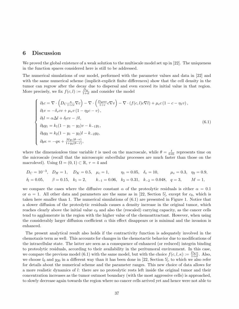
We proved the global existence of a weak solution to the multiscale model set up in [22]. The uniquenessin the function spaces considered here is still to be addressed.
The numerical simulations of our model, performed with the parameter values and data in [22] andwith the same numerical scheme (implicit-explicit finite differences) show that the cell density in thetumor can regrow after the decay due to dispersal and even exceed its initial value in that region.More precisely, we fix f(c, l) := DK
1+cl and consider the model
∂tc = ∇ ·(DC
κ1+cv∇c
)−∇ ·
(DHκv1+v c∇v
)−∇ · (f(c, l)c∇l) + µcc (1− c− η1v) ,
∂tv = −δvcv + µvv (1− η2c− v) ,
∂tl = α∆l + δlcv − βl,
∂θy1 = k1(1− y1 − y2)v − k−1y1,
∂θy2 = k2(1− y1 − y2)l − k−2y2,
∂θκ = −qκ+ My1(θ−τ)1+y2(θ−τ) ,
(6.1)
where the dimensionless time variable t is used on the macroscale, while θ = t0.01 represents time on
the microscale (recall that the microscopic subcellular processes are much faster than those on themacrolevel). Using Ω = (0, 1) ⊂ R, τ = 4 and
DC = 10−3, DH = 1, DK = 0.5, µc = 1, η1 = 0.05, δv = 10, µv = 0.3, η2 = 0.9,
δl = 0.05, β = 0.15, k1 = 2, k−1 = 0.06, k2 = 0.31, k−2 = 0.048, q = 3, M = 1,
we compare the cases where the diffusive constant α of the proteolytic residuals is either α = 0.1or α = 1. All other data and parameters are the same as in [22, Section 5], except for c0, which istaken here smaller than 1. The numerical simulations of (6.1) are presented in Figure 1. Notice thata slower diffusion of the proteolytic residuals causes a density increase in the original tumor, whichreaches clearly above the initial value c0 and also the (rescaled) carrying capacity, as the cancer cellstend to agglomerate in the region with the higher value of the chemoattractant. However, when usingthe considerably larger diffusion coefficient α this effect disappears or is minimal and the invasion isenhanced.
The present analytical result also holds if the contractivity function is adequately involved in thechemotaxis term as well. This accounts for changes in the chemotactic behavior due to modifications ofthe intracellular state. The latter are seen as a consequence of enhanced (or reduced) integrin bindingto proteolytic residuals, according to their availability in the peritumoral environment. In this case,we compare the previous model (6.1) with the same model, but with the choice f(c, l, κ) := DKκ
1+cl . Also,we choose l0 and y20 in a different way than it has been done in [22, Section 5], to which we also referfor details about the numerical scheme and the parameter ranges. This new choice of data allows fora more realistic dynamics of l: there are no proteolytic rests left inside the original tumor and theirconcentration increases as the tumor outmost boundary (with the most aggressive cells) is approached,to slowly decrease again towards the region where no cancer cells arrived yet and hence were not able to
37
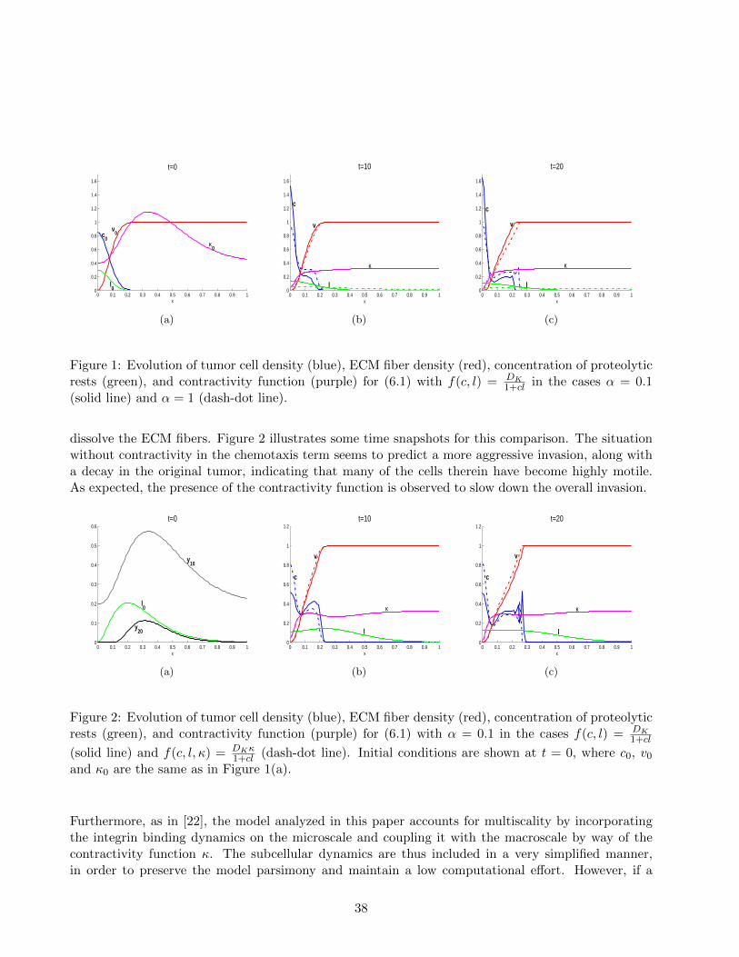
0 0.1 0.2 0.3 0.4 0.5 0.6 0.7 0.8 0.9 10
0.2
0.4
0.6
0.8
1
1.2
1.4
1.6
x
t=0
v0c
0
l0
κ0
(a)
0 0.1 0.2 0.3 0.4 0.5 0.6 0.7 0.8 0.9 10
0.2
0.4
0.6
0.8
1
1.2
1.4
1.6
x
t=10
c
v
l
κ
(b)
0 0.1 0.2 0.3 0.4 0.5 0.6 0.7 0.8 0.9 10
0.2
0.4
0.6
0.8
1
1.2
1.4
1.6
x
t=20
c
v
l
κ
(c)
Figure 1: Evolution of tumor cell density (blue), ECM fiber density (red), concentration of proteolyticrests (green), and contractivity function (purple) for (6.1) with f(c, l) = DK
1+cl in the cases α = 0.1(solid line) and α = 1 (dash-dot line).
dissolve the ECM fibers. Figure 2 illustrates some time snapshots for this comparison. The situationwithout contractivity in the chemotaxis term seems to predict a more aggressive invasion, along witha decay in the original tumor, indicating that many of the cells therein have become highly motile.As expected, the presence of the contractivity function is observed to slow down the overall invasion.
0 0.1 0.2 0.3 0.4 0.5 0.6 0.7 0.8 0.9 10
0.1
0.2
0.3
0.4
0.5
0.6
x
t=0
y10
l0
y20
(a)
0 0.1 0.2 0.3 0.4 0.5 0.6 0.7 0.8 0.9 10
0.2
0.4
0.6
0.8
1
1.2
x
t=10
c
v
l
κ
(b)
0 0.1 0.2 0.3 0.4 0.5 0.6 0.7 0.8 0.9 10
0.2
0.4
0.6
0.8
1
1.2
x
t=20
c
v
l
κ
(c)
Figure 2: Evolution of tumor cell density (blue), ECM fiber density (red), concentration of proteolyticrests (green), and contractivity function (purple) for (6.1) with α = 0.1 in the cases f(c, l) = DK
1+cl
(solid line) and f(c, l, κ) = DKκ1+cl (dash-dot line). Initial conditions are shown at t = 0, where c0, v0
and κ0 are the same as in Figure 1(a).
Furthermore, as in [22], the model analyzed in this paper accounts for multiscality by incorporatingthe integrin binding dynamics on the microscale and coupling it with the macroscale by way of thecontractivity function κ. The subcellular dynamics are thus included in a very simplified manner,in order to preserve the model parsimony and maintain a low computational effort. However, if a
38
higher level of detail is wanted for the subcellular dynamics (for instance accounting for one or moreintracellular signaling pathways relevant for proliferation, polarization, MDE production etc., whichare known to be initiated by simple integrin binding on the cell surface, see e.g., [13, 14]), then theODE system in (1.1) can be easily supplemented with the ODEs for the corresponding mass actionkinetics and the well posedness proof is expected to apply to the new (much larger) system as well.
References
[1] Alt., H.W.: Lineare Funktionalanalysis (5th ed.). Springer-Verlag, Berlin/Heidelberg, 2006
[2] Anderson, A.R.A., Chaplain, M.A.J., Newman, E.L., Steele, R.J.C., and Thompson,A.M.: Mathematical modeling of tumor invasion and metastasis. J. of Theoretical Medicine 2,129-154 (2000)
[3] Blanchet, A., Dolbeault, J., and Perthame, B.: Two-dimensional Keller-Segel model:optimal critical mass and qualitative properties of the solutions. Electron. J. Differential Equations2006, No. 44, 33pp. (2006)
[4] Cieslak, T., and Stinner, C.: Finite-time blowup and global-in-time unbounded solutions to aparabolic-parabolic quasilinear Keller-Segel system in higher dimensions. J. Differential Equations252 (10), 5832-5851 (2012)
[5] Cieslak, T., and Winkler, M.: Finite-time blow-up in a quasilinear system of chemotaxis.Nonlinearity 21, 1057-1076 (2008)
[6] Corrias, L., Perthame, B., and Zaag, H.: Global Solutions of Some Chemotaxis and An-giogenesis Systems in High Space Dimensions. Milan J. Math. 72, 1-28 (2004)
[7] van der Flier, A., and Sonnenberg, A.: Function and interactions of integrins. Cell TissueRes. 305, 285-298 (2001)
[8] Hanahan, D., and Weinberg, R.A.: Hallmarks of cancer: the next generation. Cell 144 (5),646-674 (2011)
[9] Hatzikirou, H., Basanta, D., Simon, M., Schaller, K., and Deutsch, A.: ‘Go or Grow’:the key to the emergence of invasion in tumour progression? Math. Med. Biol. 29, 49-65 (2012)
[10] Herrero, M.A., and Velazquez, J.J.L.: A blow-up mechanism for a chemotaxis model. Ann.Scuola Norm. Sup. Pisa Cl. Sci. 24, 633-683 (1997)
[11] Hieber, M., and Pruss, J.: Heat kernels and maximal Lp-Lq estimates for parabolic evolutionequations. Comm. Partial Differential Equations 22 (9-10), 1647-1669 (1997)
[12] Hillen, T., Painter, K.J., and Winkler, M.: Convergence of a cancer invasion model to alogistic chemotaxis model. Math. Models Methods Appl. Sci. 23, 165-198 (2013)
[13] Hood, J.D., and Cheresh, D.A.: Role of integrins in cell invasion and migration. NatureRev. Cancer 2, 91-100 (2002)
39
[14] Huttenlocher, A., and Horwitz A.R.: Integrins in cell migration. Cold Spring Harb. Per-spect. Biol. 3, a005074 (2011)
[15] Kelkel, J., and Surulescu, C.: A multiscale approach to cell migration in tissue networks.Math. Models Methods Appl. Sci. 22, 1150017 (2012)
[16] Ladyzenskaja, O. A., Solonnikov, V. A., and Ural’ceva, N. N.: Linear and Quasi-LinearEquations of Parabolic Type. Amer. Math. Soc. Transl., Vol. 23, Providence, RI, 1968
[17] Litcanu, G., and Morales-Rodrigo, C.: Asymptotic behavior of global solutions to a modelof cell invasion. Math. Models Methods Appl. Sci. 20, 1721-1758 (2010)
[18] Lorenz, T., and Surulescu, C., On a class of multiscale cancer cell migration models: well-posedness in less regular function spaces. preprint TU Kaiserslautern (2013), submitted
[19] Macklin, P., McDougall, S., Anderson, A.R.A., Chaplain, M.A.J., Cristini, V., andLowengrub, J.: Multiscale modelling and nonlinear simulation of vascular tumour growth. J.Math. Biol. 58, 765-798 (2009)
[20] Mallet, D.G., and Pettet, G.J.: A Mathematical Model of Integrin-Mediated HaptotacticCell Migration. Bull. Math. Biol. 68, 231-253 (2006)
[21] Marciniak-Czochra, A., and Ptashnyk, M.: Boundedness of solutions of a haptotaxismodel. Math. Models Methods Appl. Sci. 20, 449-476 (2010)
[22] Meral, G., Stinner, C., and Surulescu, C.: On a multiscale model involving cell contrac-tivity and its effects on tumor invasion. preprint TU Kaiserslautern (2013), submitted
[23] Meral, G., and Surulescu, C.: Mathematical modelling, analysis and numerical simulationsfor the influence of heat shock proteins on tumour invasion. J. Math. Anal. Appl. (2013), in print
[24] Mizoguchi, N., and Winkler, M.: Is aggregation a generic phenomenon in the two-dimensional Keller-Segel system? Preprint
[25] Osaki, K., Tsujikawa, T., Yagi, A., and Mimura, M.: Exponential attractor for achemotaxis-growth system of equations. Nonlinear Anal. TMA 51, 119-144 (2002)
[26] Porzio, M.M., and Vespri, V.: Holder Estimates for Local Solutions of Some Doubly Nonlin-ear Degenerate Parabolic Equations. J. Differential Equations 103, 146-178 (1993)
[27] Ramis-Conde, I., Drasdo, D., Anderson, A.R.A., and Chaplain, M.A.J.: Modeling theInfluence of the E-Cadherin-β Catenin Pathway in Cancer Cell Invasion: A Multiscale Approach.Biophys. J. 95, 155-165 (2008)
[28] Ramis-Conde, I., Chaplain, M.A.J., Anderson, A.R.A., and Drasdo, D.: Multi-scalemodelling of cancer cell intravasation: the role of cadherins in metastasis. Phys. Biol. 6 016008(2009)
[29] Tao, Y.: Global existence of classical solutions to a combined chemotaxis-haptotaxis model withlogistic source. J. Math. Anal. Appl. 354, 60-69 (2009)
40
[30] Tao, Y.: Global existence for a haptotaxis model of cancer invasion with tissue remodeling.Nonlinear Anal. Real World Appl. 12, 418-435 (2011)
[31] Tao, Y., and Cui, C.: A density-dependent chemotaxis-haptotaxis system modeling cancerinvasion. J. Math. Anal. Appl. 367, 612-624 (2010)
[32] Tao, Y., and Wang, M.: Global solution for a chemotactic-haptotactic model of cancer inva-sion. Nonlinearity 21, 2221-2238 (2008)
[33] Tao, Y., and Wang, M.: A combined chemotaxis-haptotaxis system: the role of logistic source.SIAM J. Math. Anal. 41, 1533-1558 (2009)
[34] Tao, Y., and Winkler, M.: A haptotaxis-chemotaxis model: the role of nonlinear diffusionand logistic source. SIAM J. Math. Anal. 43, 685-704 (2011)
[35] Tao, Y., and Winkler, M.: Boundedness and stabilization in a multi-dimensional chemotaxis-haptotaxis model. Proc. Roy. Soc. Edinburgh Sect. A, to appear
[36] Tao, Y., and Winkler, M.: Energy-type estimates and global solvability in a two-dimensionalchemotaxis-haptotaxis model with remodeling of non-diffusible attractant. Preprint
[37] Temam, R.: Navier-Stokes equations. Theory and numerical analysis. Studies in Mathematicsand its Applications. Vol. 2. North-Holland, Amsterdam, 1977
[38] Walker, C., and Webb, G.F.: Global existence of classical solutions for a haptotaxis model.SIAM J. Math. Anal. 38, 1694-1713 (2007)
[39] Wang, Z., Bordas, V., Sagotsky, J., and Deisboeck, T.S.: Simulating Cancer Growthwith Agent-Based Models, in Deisboeck, T.S. and Stamatakos, G.S. (eds.): Multiscale CancerModeling. Chapman & Hall/CRC Press, Boca Raton, 2011
[40] Webb, S.D., Sherratt, J.A., and Fish, R.G.: Alterations in proteolytic activity at low pHand its association with invasion: A theoretical model. Clinical Exp. Metastasis 17, 397-407 (1999)
[41] Winkler, M.: Boundedness in the higher-dimensional parabolic-parabolic chemotaxis systemwith logistic source. Comm. Partial Differential Equations 35, 1516-1537 (2010)
[42] Winkler, M.: Global large-data solutions in a chemotaxis-(Navier-)Stokes system modelingcellular swimming in fluid drops. Comm. Partial Differential Equations 37 (2), 319-351 (2012)
[43] Winkler, M: Finite-time blow-up in the higher-dimensional parabolic-parabolic Keller-Segel sys-tem. J. Math. Pures Appl., to appear, arXiv:1112.4156v1
[44] Zhang, L., Wang, Z., Sagotsky, J.A., and Deisboeck, T.S.: Multiscale agent-based cancermodeling. J. Math. Biol. 58, 545-559 (2009)
41