Stability

This lecture we will concentrate on

● How to determine the stability of a system represented as a transfer function

● How to determine the stability of a system represented in state-space

● How to determine system parameters to yield stability

Definitions

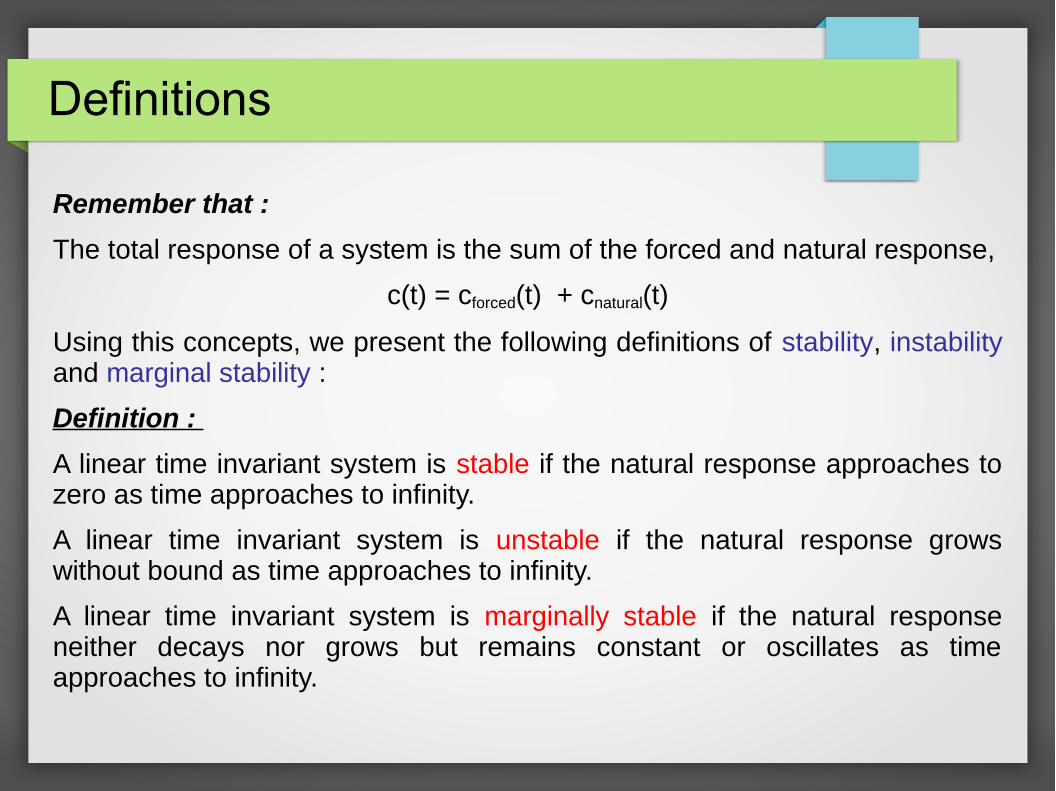
Remember that :

The total response of a system is the sum of the forced and natural response,

c(t) = cforced(t) + cnatural(t)

Using this concepts, we present the following definitions of stability, instability and marginal stability :

Definition :

A linear time invariant system is stable if the natural response approaches to zero as time approaches to infinity.

A linear time invariant system is unstable if the natural response grows without bound as time approaches to infinity.

A linear time invariant system is marginally stable if the natural response neither decays nor grows but remains constant or oscillates as time approaches to infinity.

BIBO Stability

The definitions given on the previous slide leads to a more commonly used way of defining stability for LTI systems

A system is stable if A system is stable if everyevery bounded input yields a bounded input yields a bounded output.bounded output.

We call this statement the bounded-input, bounded-output (BIBO) definition of stability.

Determining the Stability of Systems

From our previous lectures, we learned that

If the closed loop system poles are in the left-half of the s-plane and hence have a negative real part, the system is stablestable.

UnstableUnstable systems have closed loop system transfer functions with at least one pole at the right half plane and/or poles of multiplicity greater than one on the imaginary axis.

And marginally stablemarginally stable systems have closed loop transfer function with only imaginary axis poles of multiplicity 1 and poles in the left half plane.

Routh-Hurwitz Criterion

The Routh–Hurwitz stability criterion is a mathematical test that is a necessary and sufficient condition for the stability of a linear time invariant (LTI) control system.

This method enables us to investigate the stability information without the need to calculate for closed loop system poles

Basicaly the test is composed of two steps :

(1) Generate a data table called a Routh tableRouth table and

(2) interpret the Routh tableRouth table to tell how many closed loop system poles are in the left half plane, the right half plane, and on the axis.

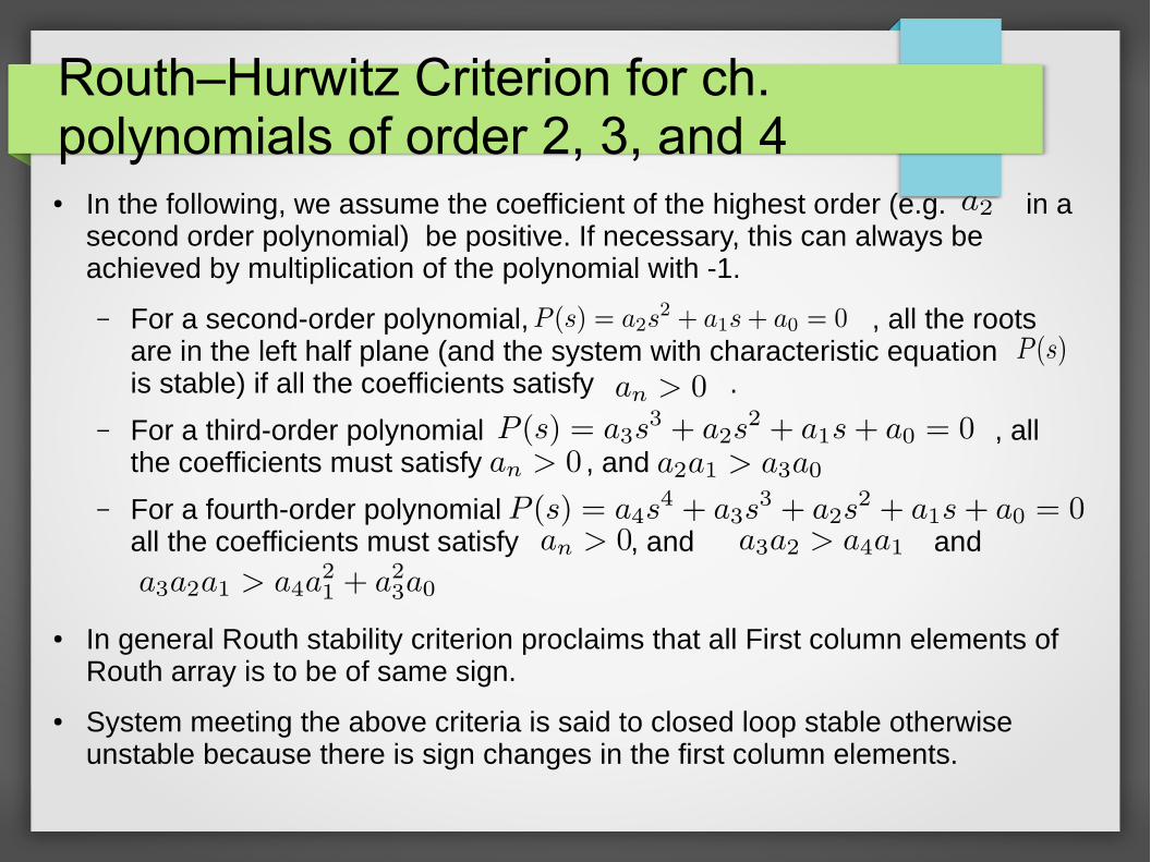
Routh–Hurwitz Criterion for ch. polynomials of order 2, 3, and 4● In the following, we assume the coefficient of the highest order (e.g. in a

second order polynomial) be positive. If necessary, this can always be achieved by multiplication of the polynomial with -1.

– For a second-order polynomial, , all the roots are in the left half plane (and the system with characteristic equation is stable) if all the coefficients satisfy .

– For a third-order polynomial , all the coefficients must satisfy , and

– For a fourth-order polynomial all the coefficients must satisfy , and and

● In general Routh stability criterion proclaims that all First column elements of Routh array is to be of same sign.

● System meeting the above criteria is said to closed loop stable otherwise unstable because there is sign changes in the first column elements.

Generation a Routh Table

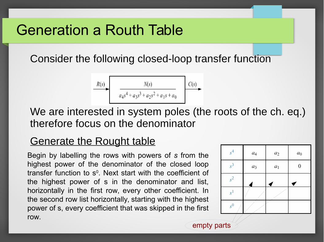
Consider the following closed-loop transfer function

We are interested in system poles (the roots of the ch. eq.) therefore focus on the denominator

Generate the Rought tableBegin by labelling the rows with powers of s from the highest power of the denominator of the closed loop transfer function to s0. Next start with the coefficient of the highest power of s in the denominator and list, horizontally in the first row, every other coefficient. In the second row list horizontally, starting with the highest power of s, every coefficient that was skipped in the first row.

empty parts

Generation a Routh Table

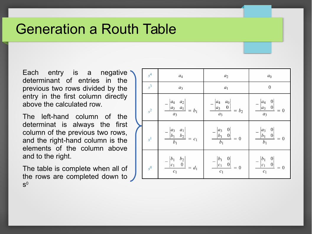
Each entry is a negative determinant of entries in the previous two rows divided by the entry in the first column directly above the calculated row.

The left-hand column of the determinat is always the first column of the previous two rows, and the right-hand column is the elements of the column above and to the right.

The table is complete when all of the rows are completed down to s0

Example #1

Investigate the stabiliy of the system with the characteristic equation given as

Solution : Form the Routh Table

The initial table Calculate the third row and simplify

Complete the overall table

is

positive

and

no sign changes

System is

STABLE

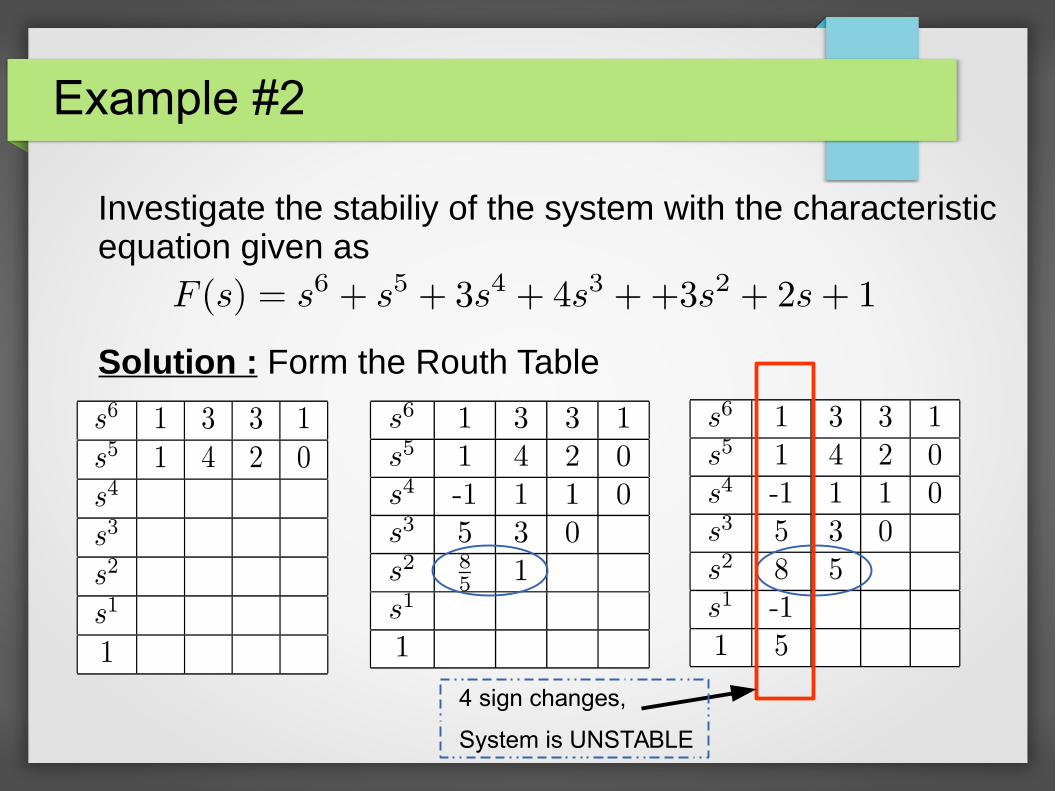
Example #2

Investigate the stabiliy of the system with the characteristic equation given as

Solution : Form the Routh Table

4 sign changes,

System is UNSTABLE

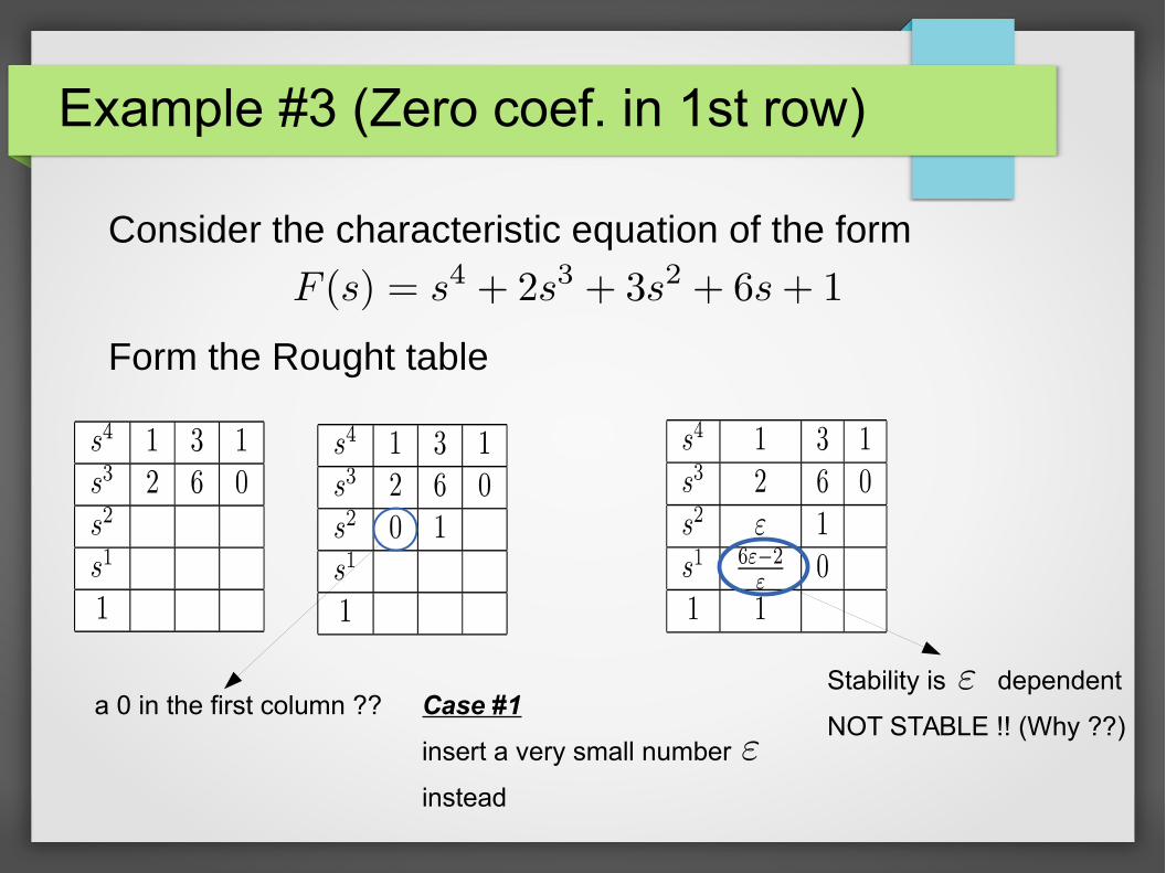
Example #3 (Zero coef. in 1st row)

Consider the characteristic equation of the form

Form the Rought table

a 0 in the first column ?? Case #1

insert a very small number

instead

Stability is dependent

NOT STABLE !! (Why ??)

Example #3

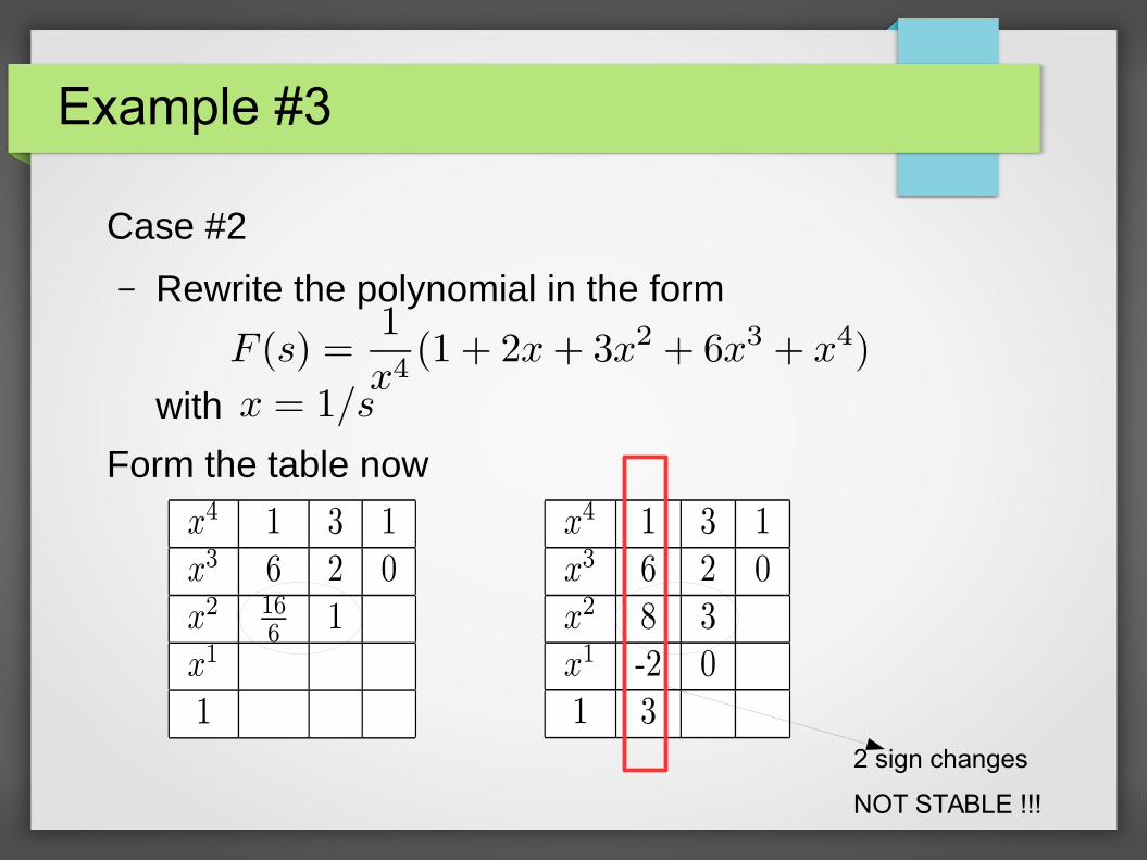
Case #2

– Rewrite the polynomial in the form

with

Form the table now

2 sign changes

NOT STABLE !!!

Example #4 (Zero Row in Table)

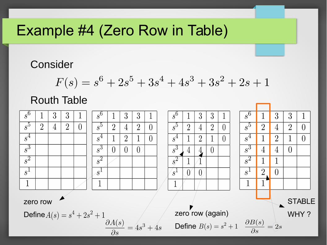
Consider

Routh Table

zero row

Define zero row (again)

Define

STABLE

WHY ?

Zero Row in the Table

● Looking further to the case of all zeros in a row :

– This can happen when a purely even or purely odd polynomial is a factor of the original polynomial

– Even polynomials only have roots that are symmetrical to the origin. This symmetry can happen only in 3 conditions

● The roots are symmetric and pure real● The roots are symmetric and pure imaginary● The roots are quadrantal.

Example #5 (variable gain)

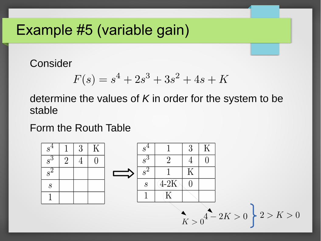
Consider

determine the values of K in order for the system to be stable

Form the Routh Table

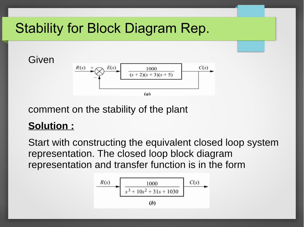
Stability for Block Diagram Rep.

Given

comment on the stability of the plant

Solution :

Start with constructing the equivalent closed loop system representation. The closed loop block diagram representation and transfer function is in the form

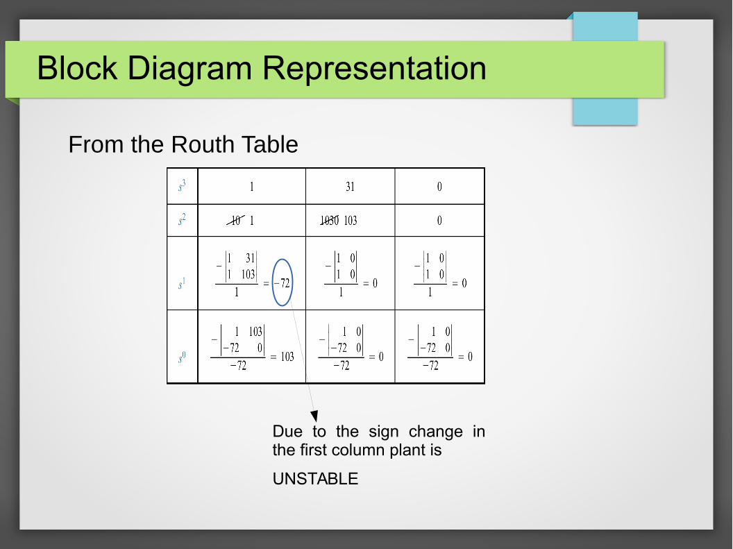
Block Diagram Representation

From the Routh Table

Due to the sign change in the first column plant is

UNSTABLE

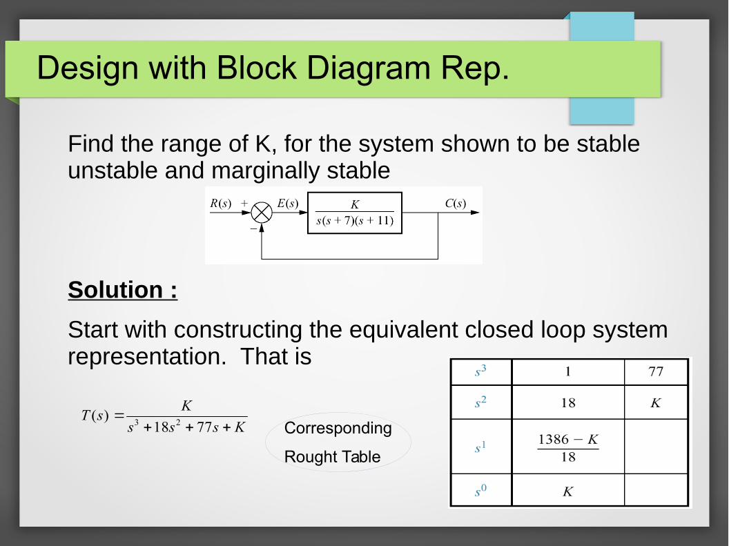
Design with Block Diagram Rep.

Find the range of K, for the system shown to be stable unstable and marginally stable

Solution :

Start with constructing the equivalent closed loop system representation. That is

Ksss

KsT

7718)(

23 Corresponding

Rought Table

● Since K assumed positive, we see that all elements in the first column are always positive except the s1 row. This entry can be positive, zero, or negative, depending upon the value of K.

● If K<1386, all terms in the first column will be positive, and since there are no sign changes, the system will have three poles at the left half plane and be stable.

● If K>1386, the s1 term in the first column is negative. There are two sign changes, indicating that the system has two right half plane poles and one left half plane pole, which makes the system unstable.

● If K=1386, we have an entire row of zeros, which colud signify jω poles. Returning the s2 row and replacing K with 1386, we form the even polynomial P(s)=18s2+1386. Differetiating with respect to s, we obtain dP(s)/ds=36s .

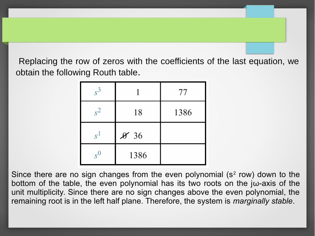
Replacing the row of zeros with the coefficients of the last equation, we obtain the following Routh table.

Since there are no sign changes from the even polynomial (s2 row) down to the bottom of the table, the even polynomial has its two roots on the jω-axis of the unit multiplicity. Since there are no sign changes above the even polynomial, the remaining root is in the left half plane. Therefore, the system is marginally stable.

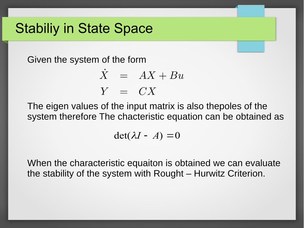
Stabiliy in State Space

Given the system of the form

The eigen values of the input matrix is also thepoles of the system therefore The chacteristic equation can be obtained as

When the characteristic equaiton is obtained we can evaluate the stability of the system with Rought – Hurwitz Criterion.

0)det( AI

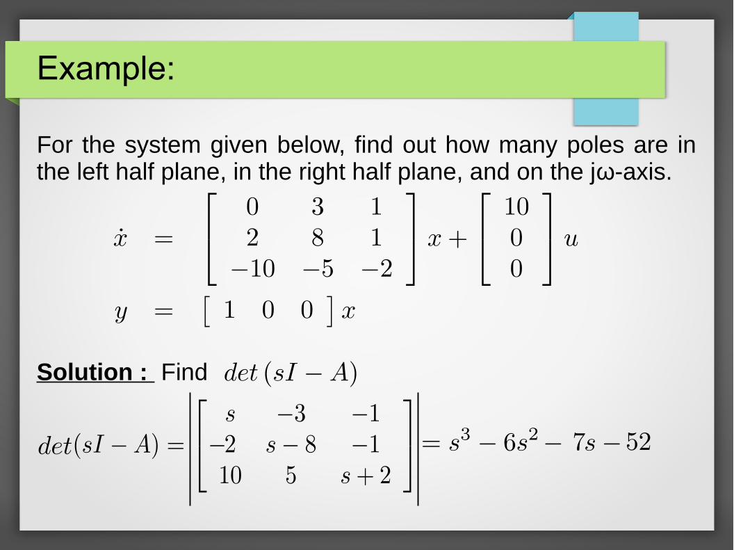
Example:

For the system given below, find out how many poles are in the left half plane, in the right half plane, and on the jω-axis.

Solution : Find

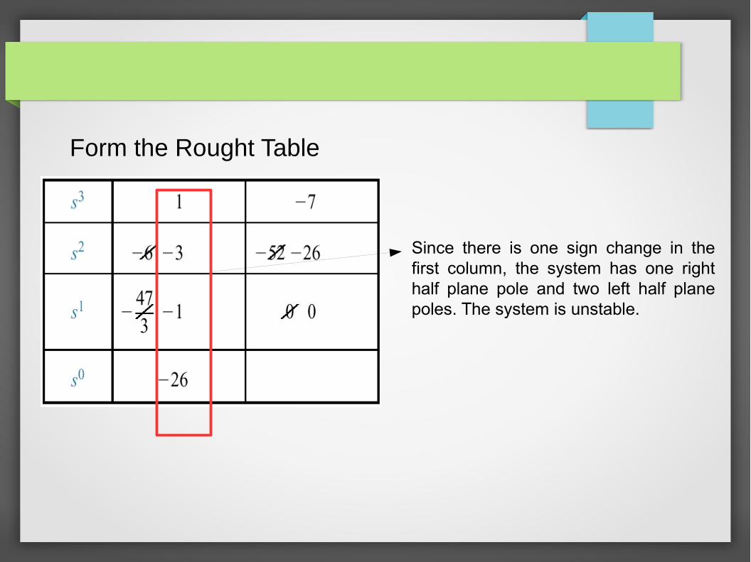
Form the Rought Table

Since there is one sign change in the first column, the system has one right half plane pole and two left half plane poles. The system is unstable.