statistical analysis of the effects of prior load on fracture

$: Statistical analysis of the effects of prior load on fracture$
Engineering Fracture Mechanics 74 (2007) 2148–2167

www.elsevier.com/locate/engfracmech

Statistical analysis of the effects of prior load on fracture

D.J. Smith *, J.D. Booker

Department of Mechanical Engineering, University of Bristol, Queen’s building, Bristol BS8 1TR, UK

Received 9 June 2006; received in revised form 25 September 2006; accepted 20 October 2006Available online 4 December 2006

Abstract

Collated fracture data for three steels, A533B, A508 and BS1501, and an Aluminium alloy, 2650, were examined toassess the statistical significance of the effect of prior loading on subsequent fracture. Weibull statistical and probabilisticanalysis was used throughout. Two prior loading conditions were examined; one associated with warm pre-stress, and asecond using pre-compression. For the former, prior loading resulted in an increase in the mean toughness together with anincrease in the shape parameter and a decrease in variability compared to the as-received material. In contrast, when priorloading involved out-of-plane compressive loading (or side-punching) statistical evidence revealed that there was a reduc-tion in toughness together with a decrease in the shape parameter and an increase in variability. Two numerical modelswere applied to steel data and were able to predict the overall trends obtained from the experiments, but could not repro-duce accurately the experimental statistical distributions.� 2006 Elsevier Ltd. All rights reserved.

Keywords: Prior load history; Statistical analysis; Fracture

1. Introduction

The operational characteristics of many practical engineering components are such that they experienceoverload and underload events rather than their design conditions. It is also common practice in many engi-neering sectors to subject components to proof testing as a measure of quality assurance for future use. Prooftesting a component consists of applying a load greater than it is likely or designed to experience during ser-vice. Its main aim has been, and continues, to be to assure the quality of component or structural fabricationby revealing manufacturing ‘‘defects’’. These ‘‘defects’’ may arise from incorrect design, poor workmanship oreven more drastically using incorrect material. This feature of proof testing is often viewed as a qualitativemeasure of the worth of the component. Proof testing is just one example of subjecting a component to loadsgreater than expected from design calculations. There are naturally events during the life of the componentwhere additional loads, greater (or even lower) than expected, are experienced. Examples are overload andunderload cycles experienced by an aircraft wing and marine structures subjected to overloading from high

0013-7944/$ - see front matter � 2006 Elsevier Ltd. All rights reserved.

doi:10.1016/j.engfracmech.2006.10.011

* Corresponding author. Tel.: +44 1179288212; fax: +44 1179294423.E-mail address: [email protected] (D.J. Smith).

mailto:[email protected]

Nomenclature

B specimen thicknesscdf cumulative distribution functionCF cool-fractureC(T) compact tension specimenLOS level of significanceLUCF single-load-unload-cool-fractureMCS Monte-Carlo simulationpdf probability density functionPUC punch-unload-cool-fracturePUF punch-unload-fractureRNB round notched bar specimenSEN(B) single edge notched bend specimenWPS warm pre-stressingCv coefficient of variationKIc plane strain fracture toughnessKmin, rmin, Rmin expected minimum valuesK0, r0, R0 characteristic valuesKwps applied elastic stress intensity factor during WPSp probabilityPf cumulative failure probabilityP1 probability that LUCF provides an increase in toughnessP2 probability that PUCF provides a decrease in toughnessm, b shape parametersl mean valueR net section fracture stressr standard deviationr1 maximum principal stressrw Weibull stressrmin minimum stressru characteristic stressV0 reference volumeVp near crack tip plastic volume

D.J. Smith, J.D. Booker / Engineering Fracture Mechanics 74 (2007) 2148–2167 2149

sea states. Higher operational demands on power generation equipment may also introduce higher loads andtemperatures than normally seen during standard service conditions. Another more extreme example is a faultcondition called pressurised thermal shock in nuclear reactor pressure vessels. This condition arises when thereis severe overcooling of the reactor vessel.

Prior loading events are well known to influence the fracture and fatigue behaviour of materials. For exam-ple, subjecting a component to a prior overload at a temperature higher than the subsequent operating tem-perature is generally called warm pre-stressing (WPS). The bulk of the WPS studies were performed to studyfracture toughness of low alloy ferritic steels that exhibit a fracture mechanism that changes from brittle toductile with increasing temperature. If the component contains a defect, experimental results demonstrate thatthe WPS event enhances the cleavage fracture toughness of the material [1,2]. The majority of the studies onthe influence of overloading on subsequent fatigue crack growth concentrate on retardation of crack growthrate. The effect is well documented [3], with the main focus concentrating on how overload affects crackopening.

In both cases, WPS and overloading of fatigue cracks, prior loading events lead to three possible contrib-uting factors influencing subsequent fracture behaviour. One factor is the generation of residual stresses at the

2150 D.J. Smith, J.D. Booker / Engineering Fracture Mechanics 74 (2007) 2148–2167

crack. A second factor is prior straining changes the material behaviour, and finally the crack shape is mod-ified (e.g. crack tip blunting) as a consequence of prior loading. All three contributions are difficult to quantify,although in the case of WPS, Smith et al. [1,2] argue that the most important contribution to the enhancementin toughness arises from the presence of compressive residual stresses. For underloading, where the remoteapplied stress maybe compressive, a tensile residual stress is generated at crack tips or notch roots. In suchcases, the presence of tensile residual stress will lower the fracture toughness or increase the growth rate offatigue cracks.

The experimental data examined in this paper was generated to explore the effects of prior load history onthe fracture toughness of steels and an aluminium alloy. This is done in the context that materials properties,such as fracture toughness, exhibit variability because of anisotropy, inhomogenity, chemical composition,impurities and defects [4,5]. All materials are, of course, processed in some way so that they are in some usefulfabrication condition. The level of variability in material properties associated with the lack of control of pro-cessing parameters can also be a major contribution. Fracture toughness exhibits more statistical variationthan other material properties. This is especially pronounced around the brittle-ductile temperature transitionregion, this region varying by as much as 50 �C for the same batch of steel [5]. The coefficient of variation (Cv)for fracture toughness of steels ranges from 0.1 to 0.2 [5].

Earlier attempts to examine the statistical analyses of the effect of prior loading (in particular WPS) on frac-ture toughness have been made by Fowler et al. [6] and Wallin [7]. Fowler et al. [6] proposed that the Weibullfailure probability after WPS could be modified using a model developed by Chell [8]. However, as pointed outby Wallin [7], this model does not change the Weibull shape parameter, and a simpler WPS was proposed [7].This is examined further in this paper.

Our main purpose in this paper is to examine collated experimental evidence to test whether prior loadingevents do influence fracture toughness or fracture stress. If they do, we examine how the statistical parametersfor the virgin or ‘‘as-received’’ material are modified. Two forms of prior loading are examined; the first con-sists of a particular form of WPS, called the LUCF cycle and the second is called side-punching of specimens.This is a technique used by Mahmoudi et al. [9] to introduce tensile residual stresses into fracture specimens.The paper first summarises experimental data from our earlier work. We then describe the statistical treatmentof the results and undertake a series of statistical tests to assess the level of confidence that the influence ofprior loading is statistically significant. The results are also discussed in the context of number of models (ana-lytical and numerical) that predict how prior loading changes the fracture response of a material.

2. Experimental data

Experimental results for statistical analysis were collated from our own test programmes, and are confinedto three pressure vessel steels, A533B, BS1501, A508 and an aluminium alloy, Al2650. Fracture tests were car-ried out on each metallic alloy in the as-received state. Further test samples were subjected to two prior loadevents followed by fracture of the samples. The geometry of the test specimens is shown in Fig. 1, with sche-matics of the load cycles shown in Fig. 2. Fig. 2a shows the basic load cycle to obtain the as-received fracturetoughness. One type of prior loading was to load pre-cracked specimens in tension at room temperature,unload, cool the specimen and then finally load to fracture at the lower temperature, shown as the LUCF cyclein Fig. 2b. In the LUCF cycle the prior loading is in the same plane as the final fracture load. The second typeof prior loading, Fig. 2c, consisted of subjecting specimens to side-punching (pre-compression). Here, priorloading out-of-plane occurs in compression relative to the final applied fracture load and is designated thePUCF cycle.

In the following the basic features of the material, test geometry and conditions for prior loading are sum-marised. The fracture toughness, K, for tests using SEN(B) and C(T) specimens, was determined from themaximum load at fracture using standard formulae [14].

2.1. A533B steel

Experimental data sets from two batches of A533B steel were collated. Set 1 from an A533B steel studied bySmith and Garwood [10], Fowler [11], and Smith et al. [1,2]. Data for Set 2 correspond to a A533B steel

Fig. 1. Specimen geometries analysed showing direction of loading for fracture.


studied by Ingham et al. [12] and Mirzee-Sisan et al. [13]. The chemical compositions for the two casts areshown in Table 1.

For A533B steel-set 1, single edge notch bend, SEN(B) and compact tension, C(T) specimens were tested.The thickness B of SEN(B) specimens was 50 mm, while for C(T) specimens B = 25 mm and 6 mm were studied.Tests in the as-received state were simply cooled and then fractured (CF). This cycle is illustrated in Fig. 2a.The prior load condition was a load-unload-cool-fracture (LUCF) cycle, Fig. 2b. All prior loading was con-ducted at room temperature, (20 �C), followed by cooling then subsequent fracture at a temperature to causecleavage fracture. The fracture temperatures were �170 �C and �100 �C.

All test results for A533B steel are shown in Fig. 3. Fig. 3a shows results for SEN(B) tests with B = 50 mmand C(T) tests with B = 6 mm at �170 �C. Test results for SEN(B) specimens with B = 50 mm at �100 �C areshown in Fig. 3b. In both figures cumulative failure probability, Pf was calculated from experimental resultsusing

P f ¼i� 0:5

Nð1Þ

where N and i are the total number of specimens and the order number, respectively.For set 2, 25 mm thick C(T) and 10 mm thick SEN(B) specimens were tested in as-received state (CF) at

�170 �C and �150 �C and after prior loading. This prior loading consisted of side-punching at room tem-perature or out-of-plane compressive loading. This prior loading is intended to introduce tensile residualstresses into the region adjacent to the crack tip. Side punching was followed by cooling, then loading tofracture, punch-unload-cool-fracture (PUCF). This cycle is illustrated in Fig. 2c. The C(T) and SEN(B)specimens were fractured at �170 �C and �150 �C, respectively. Test results are shown in Fig. 3c. All spec-imen fracture surfaces for sets 1 and 2 revealed that brittle fracture was associated with a cleavage failuremechanism.

Load Load

Temperature

C

F

Cool-Fracture

Displacement

Temperature

Load

LU

C

F

Load-Unload-Cool-Fracture

Displacement

Load

Temperature

Load

PU

C

F

Punch-Unload-Cool-Fracture

Displacement

Load

Fig. 2. Load and temperature cycles.

Table 1Chemical compositions (wt%) of A533B class 1 steel

(a) Set 1 A533B Class 1 pressure vessel steel (from [10])

Element C S P Si Mn Ni Cr Mo Cowt% 0.18 0.005 0.006 0.240 1.41 0.56 0.180 0.480 0.01

Element V Cu Nb Ti Al Sn As Nb Bwt% <0.002 0.120 <0.002 <0.018 0.030 0.004 0.019 < 0.010 <0.0003

(b) Set 2 A533B Class 1 Pressure Vessel Chemical composition of A533B material (from [12])

Element C Mn Mo Ni Si Cr S P Cu Alwt % 0.21 1.44 0.48 0.67 0.28 0.18 0.005 0.006 0.05 0.021


2.2. BS 1501 steel

The tests conducted on this steel were also summarised by Smith et al. [1]. The chemical composition forthis steel is shown in Table 2. C(T) and SEN(B) tests were conducted by Smith and Garwood [15] and Fowler

Fracture Toughness, K, MPam0.50 50 100 150 200

0

20

40

60

80

100

SEN(B)50, CF,-170SEN(B)50, LUCF, -170C(T)25, LUCF, -170C(T)6, CF, -170C(T)6, LUCF, -170C(T)25, CF, -170

100 120 140 160 180 200 2200

20

40

60

80

100

SEN(B)50,CF, -100SEN(B)50, LUCF, -100

20 40 60 80 100

Fai

lure

Pro

babi

lity,

Pf,

%

0

20

40

60

80

100

C(T)25, CF, -170

C(T)25, PUCF, -170SEN(B)10, CF, -150

SEN(B)10, PUCF, -150

Fai

lure

Pro

babi

lity,

P f, %

Fai

lure

Pro

babi

lity,

Pf,

%

Fracture Toughness, K, MPam0.5


Fig. 3. Experimental results and fitted Weibull curves for A553B Steels: (a) CF and LUCF fracture tests at �170 �C, (b) CF and LUCFfracture tests at �100 �C, (c) CF and PUCF tests at �170 �C and �150 �C.


[11]. Similar to the studies on A533B steel, SEN(B) and C(T) specimens were subjected to CF and LUCFcycles, where, in all cases, the load and unload parts of the cycle were conducted at room temperature, andthe low temperature fracture undertaken at temperatures ranging from �120 to �50 �C. All specimen fracturesurfaces revealed that brittle fracture was associated with a cleavage failure mechanism. Test results are shownin Fig. 4a and b.

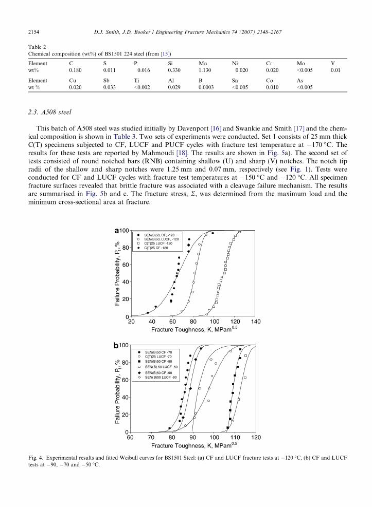
Table 2Chemical composition (wt%) of BS1501 224 steel (from [15])

Element C S P Si Mn Ni Cr Mo Vwt% 0.180 0.011 0.016 0.330 1.130 0.020 0.020 <0.005 0.01

Element Cu Sb Ti Al B Sn Co Aswt % 0.020 0.033 <0.002 0.029 0.0003 <0.005 0.010 <0.005


2.3. A508 steel

This batch of A508 steel was studied initially by Davenport [16] and Swankie and Smith [17] and the chem-ical composition is shown in Table 3. Two sets of experiments were conducted. Set 1 consists of 25 mm thickC(T) specimens subjected to CF, LUCF and PUCF cycles with fracture test temperature at �170 �C. Theresults for these tests are reported by Mahmoudi [18]. The results are shown in Fig. 5a). The second set oftests consisted of round notched bars (RNB) containing shallow (U) and sharp (V) notches. The notch tipradii of the shallow and sharp notches were 1.25 mm and 0.07 mm, respectively (see Fig. 1). Tests wereconducted for CF and LUCF cycles with fracture test temperatures at �150 �C and �120 �C. All specimenfracture surfaces revealed that brittle fracture was associated with a cleavage failure mechanism. The resultsare summarised in Fig. 5b and c. The fracture stress, R, was determined from the maximum load and theminimum cross-sectional area at fracture.

20 40 60 80 100 120 1400

20

40

60

80

100SEN(B)50, CF, -120SEN(B)50, LUCF, -120C(T)25 LUCF -120C(T)25 CF -120

60 70 80 90 100 110 1200

20

40

60

80

100SEN(B)50 CF -70C(T)25 LUCF -70SEN(B)50 CF -50

SEN(B) 50 LUCF -50

SEN(B)50 CF -90SEN(B)50 LUCF -90


Fai

lure

Pro

babi

lity,

Pf,

%


Fai

lure

Pro

babi

lity,

Pf,

%

Fig. 4. Experimental results and fitted Weibull curves for BS1501 Steel: (a) CF and LUCF fracture tests at �120 �C, (b) CF and LUCFtests at �90, �70 and �50 �C.

Table 3Chemical composition (wt%) of A508B class 3 steel (from [16])

Element C S P Si Mn Ni Cr Mowt% 0.160 0.007 0.004 0.220 1.340 0.670 0.170 0.510

Element V Cu Sb Ti Al Sn As Nbwt% <0.010 0.060 0.004 <0.010 0.010 0.004 0.019 <0.010

0 20 40 60 80 100 120 140 160 1800

20

40

60

80

100

A508 C(T)25, CF, -170A508 C(T)25, PUCF, -170A508 C(T)25, LUCF, -170

Fracture Stress, MPa1000 1200 1400 1600 1800 20000

20

40

60

80

100

A508, RNB shallow, CF, -150A508, RNB shallow, LUCF, -150A508, RNB shallow, CF, -120A508, RNB shallow, LUCF, -120

Fracture stress, MPa200 400 600 800 1000 1200 1400 1600 1800 20000

20

40

60

80

100A508, RNB sharp, CF, -150

A508, RNB sharp, LUCF, -150

Fracture Toughness, MPam0.5

Fai

lure

Pro

babi

lity,

Pf,

%F

ailu

re P

roba

bilit

y, P

f, %

Fai

lure

Pro

babi

lity,

Pf,

%

Fig. 5. Experimental results and fitted Weibull curves for A508 Steel: (a) CF, PUCF and LUCF fracture tests at �170 �C, (b) CF andLUCF shallow notched bar tests at �150 and �120 �C, and (c) CF and LUCF sharp notched bar tests at �150 �C.


Table 4Chemical composition (wt%) for aluminium alloy 2650 (from [19])

Element Cu Mg Fe Si Mn Ni Tiwt% 2.74 1.74 0.1 0.4 0.34 0.20 0.09

10 15 20 25 30 35 400

20

40

60

80

100

Al2650, C(T)15, F, 20Al2650, C(T)15, PUF, 20

Fracture Toughness, K, MPam 0.5

Fai

lure

Pro

babi

lity,

Pf,

%

Fig. 6. Experimental and fitted Weibull curves to Aluminium 2650 fracture and PUF tests.


2.4. Aluminium alloy Al 2650

The aluminium alloy, Al2650 (whose chemical composition is shown in Table 4) was studied initially byLacarac et al. [19] to examine the growth of fatigue cracks in cold worked holes, and by Mahmoudi [18]and Mirzaee-Sisan et al. [20] to study the influence of residual stress on fracture toughness. For the latter stud-ies, 15 mm thick C(T) specimens were extracted from the supplied plate. One set of samples were fractured atroom temperature and another set subjected to side-punching at room temperature, unloaded and thenreloaded to cause fracture, again at room temperature (punch-unload-fracture, PUF, cycle). Test results areshown in Fig. 6. All specimen fracture surfaces revealed that ductile fracture was associated with microvoidcoalescence. All specimens failed by instability following ductile crack growth.

3. Statistical analyses

3.1. Statistical characterisation of fracture toughness and stress

The collated experimental fracture toughness data were fitted using a 3-parameter Weibull distribution,where the 3-parameter Weibull probability density function (pdf), f(K) is given by

f ðKÞ ¼ bK0 � Kmin

� �K � Kmin

K0 � Kmin

� �b�1

exp � K � Kmin

K0 � Kmin

� �b !

; K P Kmin ð2Þ

where K is the fracture toughness (variate), Kmin is the expected minimum value, K0 is the characteristic valueand b is the shape parameter.

This flexible distribution is commonly used to model data where a high degree of skew or where non-zerothreshold may be anticipated, particularly for strength of brittle materials, such as ceramics, and fatigueendurance of metals. The shape of the Weibull distribution is dictated by the shape parameter, b. This valueis a measure of the variability of the sample data. Low values of b, for example 1 or 2, relate to high variabilityin the sample data. For b = 3.44, this indicates that data are approximately near-Normal [21]. A high b (5 or 6)indicates low variability and therefore in terms of a material property, more consistency. If an improved esti-mate for the mean and standard deviation of a set of data is the goal, it has been cited that determining theWeibull parameters and then converting to Normal parameters using suitable transformation equations is alsorecommended [22].


An efficient way of using all the information and judgment available in the estimation of the parameters ofany distribution type is the use of the ‘linearised’ cumulative frequency. Essentially, this involves convertingthe non-linear data points describing the cumulative frequency so they may be described by a linear equation.For the 3-parameter Weibull distribution, this involves changing both axis variables by applying natural logoperators. A straight line through the plotted data points can then be determined using the least squares tech-

nique to estimate the linear equation parameters from which the 3-Weibull distributional parameters can thenbe determined. The mathematical and statistical process is called linear rectification [23]. The expected mini-mum value parameter, Kmin is automatically found from an algorithm to find the linear relationship with thehighest correlation coefficient. When the parameters have been determined for each set of data, the failureprobability can be then be described by the cumulative distribution function (cdf), F(K) or failure probabilityPf , for the 3-parameter Weibull distribution given by

P f ½K� ¼ 1� exp � K � Kmin

K0 � Kmin

� �b !

ð3Þ

For the tests on round notched bars, experimental data were expressed in terms of fracture stress, R, and con-sequently a similar equation to [3] was used

P f ½R� ¼ 1� exp � R� Rmin

R0 � Rmin

� �b !

ð4Þ

where Rmin and R0 are the minimum and characteristic stress values, respectively.The results of the fitting to the experimental data are given in Table 5 by material type, geometry, test con-

ditions, sample size, Weibull distribution parameters, equivalent Normal distribution parameters, and coeffi-cient of variation. The coefficient of variation, Cv, for each sample is calculated by dividing the standarddeviation, r, by the mean, l. Also Figs. 3–6 illustrate the curves described by Eqs. (3) or (4) using the Weibullparameters shown in Table 5.

Representative probability density functions (pdfs) derived from the experimental data are illustrated in Figs.7–10. With the LUCF cycle applied to A533B steel (set 1), Fig. 7 shows that there is not only an increase in thetoughness compared to the as-received condition but also a change in the form of the distribution. For example,for SEN(B) specimens fractured at�170 �C the shape parameter, b, changes from 4.2 for the as-received materialto 6.3 after the LUCF cycle, indicating a reduction in the spread of test results after prior loading.

The nature of the distribution of the fracture results after PUCF is however different compared to LUCFresults. Figs. 8 and 9 illustrate that for cleavage fracture in steel the PUCF distribution becomes skewed to theleft without much change in the overall distribution. In contrast, for the aluminium alloy subjected to thePUCF cycle, Fig. 10 there is both a considerable decrease in the average toughness and a skewed distribution.

3.2. Probability of fracture toughness increase or decrease

There were essentially two prior loading methods used in the experimental studies. One method involvedprior loading at room temperature followed by cooling and brittle fracture at low temperature (LUCF). Asthe experimental results illustrate in Figs. 3–5, this resulted in an increase in toughness. The second methodapplied to the pressure vessel steels was side-punching followed by cooling and brittle fracture, PUCF, witha resulting small decrease in fracture toughness, Figs. 3c and 5. In contrast, when the PUF cycle was applied toAl2650 at room temperature, there was a dramatic decrease in toughness.

The probability, P1, of whether LUCF does provide a benefit to the toughness in a significantly large pro-portion of the population is determined from the quotient of the pdfs for the LUCF fracture toughness,KIcLUCF

and, the original condition fracture toughness, KIcCF:

P 1 ¼ pKIcLUCF

KIcCF

P 1

� �ð5Þ

Table 5Fitted Weibull statistical parameters

Material, specimen type, thickness andtest condition

Number ofspecimens

Weibullparameters

Normalparameters

Coefficient ofvariation, Cv

Units Kmin andK0 = MPa m0.5

r andl = MPa m0.5

(a) A533B Steel

A533B Set 1, C(T) 25 CF �170 3 K0 = 64.4 l = 59.3 0.253b = 3.076 r = 15.0Kmin = 16.8

A533B Set 1 C(T) 25 LUCF �170 12 K0 = 90.1 l = 85.2 0.282b = 1.748 r = 24.1Kmin = 44.8

A533B Set 1 C(T) 6 CF �170 10 K0 = 124.0 l = 123.4 0.305b = 1.037 r = 37.7Kmin = 84.5

A533B Set1 C(T) 6 LUCF �170 17 K0 = 168.6 l = 156.3 0.183b = 5.774 r = 28.6Kmin = 11.5

A533B Set 1 SEN(B) 50 CF �170 14 K0 = 64.1 l = 58.7 0.237b = 4.219 r = 13.9Kmin = 5.9

A533B Set 1 SEN(B) 50 LUCF �170 14 K0 = 104.7 l = 97.8 0.162b = 6.265 r = 15.8Kmin = 11.3


A533B Set 1 SEN(B) 50 LUCF �100 12 K0 = 197.3 l = 189.1 0.100b = 6.327 r = 18.9Kmin = 84.7

A533B Set 2 C(T) 25 CF �170 12 K0 = 48.5 l = 45.6 0.173b = 3.615 r = 7.9Kmin = 19.7

A533B Set 2 C(T) 25 PUCF �170 12 K0 = 43.6 l = 41.4 0.244b = 1.840 r = 10.1Kmin = 23.6


A533B Set 2 SEN(B) 10 PUCF �150 10 K0 = 57.1 l = 54.8 0.259b = 1.526 r = 14.2Kmin = 33.8

(b) BS1501 Steel

BS1501 C(T)25 CF-120 3 K0 = 67.6 l = 67.3 0.153b = 1.063 r = 10.3Kmin = 56.4

BS1501 C(T)25 LUCF �120 23 K0 = 112.2 l = 109.2 0.071b = 4.096 r = 7.8Kmin = 80.5

BS1501 SEN(B)50 CF �120 14 K0 = 71.0 l = 6 5.1 0.231b = 4.415 r = 15.0Kmin = 5.6

BS1501 SEN(B)50 LUCF �120 9 K0 = 84.4 l = 81.5 0.064b = 6.091 r = 6.7Kmin = 45.9

BS1501 SEN(B)50 CF �70 12 K0 = 87.5 l = 85.9 0.042b = 5.643 r = 5.6Kmin = 68.1


Table 5 (continued)

Material, specimen type, thickness andtest condition

Number ofspecimens

Weibullparameters

Normalparameters

Coefficient ofvariation, Cv

Units Kmin andK0 = MPa m0.5

r andl = MPa m0.5

BS1501 C(T)25 LUCF �70 7 K0 = 100.0 l = 89.3 0.072b = 4.899 r = 11.9Kmin = 66.9





(c) A508 Steel

A508 C(T)25 CF �170 8 K0 = 53.1 l = 50.0 0.231b = 2.258 r = 11.6Kmin = 25.4

A508 C(T)25 PUCF �170 8 K0 = 42.7 l = 42.7 0.273b = 1.003 r = 11.6Kmin = 31.3

A508 C(T) 25 LUCF �170 8 K0 = 122.7 l = 116.6 0.113b = 5.477 r = 14.3Kmin = 47.4

Units R0 = Rmin = MPa r = l = MPa

A508 RNB Shallow CF �150 9 R0 = 1413.1 l = 1379.0 0.059b = 5.322 r = 81.2Rmin = 997.0

A508 RNB Shallow LUCF �150 8 R0 = 1403.7 l = 1400.2 0.031b = 0.704 r = 43.8Rmin = 1355.7

A508 RNB Shallow CF �120 10 R0 = 1589.6 l = 1543.4 0.076b = 4.273 r = 116.9Rmin = 1094.7

A508 RNB Shallow LUCF �120 10 R0 = 1621.3 l = 1576.331 0.066b = 5.980 r = 104.2Rmin = 1030.7

A508 RNB Sharp CF �150 9 R0 = 1174.6 l = 1059.6 0.273b = 4.388 r = 289.6Rmin = -79.7

A508 RNB Sharp LUCF �150 8 R0 = 1401.9 l = 1364.8 0.065b = 5.222 r = 88.7Rmin = 955.6

(d) Al2650

Al2650 C(T) 25 F 20 10 K0 = 31.7 l = 31.2 0.044b = 5.144 r = 1.4Kmin = 25.0

Al2650 C(T) 25 PUCF 2010 K0 = 15.2 l = 15.2 0.176

b = 1.011 r = 2.7Kmin = 12.5


Fracture Toughness, KIC, MPam0.50 20 40 60 80 100 120 140 160

PD

F

0.00

0.01

0.02

0.03

0.04 SEN(B)50 CF,-170 Experimental

SEN(B)50 LUCF,-170 Experimental

SEN(B) 50 LUCF,-170 Predicted

Fig. 7. Comparison of experimental and predicted probability distributions for A533B steel subjected to CF and LUCF conditions.

PD

F

0.00

0.01

0.02

0.03

0.04

0.05

0.06C(T)25, CF, -170 ExperimentalC(T)25, PUCF, -170 ExperimentalC(T)25, PUCF, -170 Predicted

0 20 40 60 80 100Fracture Toughness, KIC, MPam0.5

Fig. 8. Comparison of experimental and predicted probability distributions for A533B steel subjected to CF and PUCF conditions.

0 50 100 150 200

PD

F

0.00

0.02

0.04

0.06C(T)25 CF ExperimentalC(T)25 LUCF ExperimentalC(T)25 LUCF PredictedC(T)25 PUCF ExperimentalC(T)25 PUCF Predicted

Fracture Toughness, MPam0.5

Fig. 9. Comparison of experimental and predicted probability distributions for A508 steel subjected to CF, LUCF and PUCF conditions.


Conversely, the probability, P2, of whether PUCF (or PUF) does decrease the toughness compared to theoriginal fracture toughness is

0 10 20 30 40

PD

F

0.00

0.05

0.10

0.15

0.20

0.25

0.30

0.35 C(T) 25 FractureC(T) 25 PUF


Fig. 10. Comparison of experimental and predicted probability distributions for Aluminium alloy 2650 steel subjected to fracture andPUF conditions.


P 2 ¼ pKIcPUCF

KIcCF

6 1

� �ð6Þ

Monte Carlo Simulation (MCS) was used to determine the mean, l and standard deviation, r for the quotientsin Eqs. (5) and (6) [23]. Once a new quotient pdf was determined, the final probability that a ratio of greater orless than unity has been achieved was approximated from standard normal distribution (SND) tables [23]. Thechange in the coefficient of variation, Cv, from the CF to the LUCF or PUCF cycles may also be determinedfrom Table 5.

The change in b gives an indication whether variability has increased (#) or decreased (") from the originalvalue determined from the CF testing regime. All results are shown in Table 6. With the exception of one case(A508 steel RNB specimens with shallow notches tested at �150C) the shape parameter, b increases (i.e. thespread of results becomes lower) after the LUCF load cycle. In contrast, b decreases (i.e. the spread of dataincreases) after the PUCF cycle.

3.3. Hypothesis testing

Next we need to speculate whether the effects of prior loading on the fracture toughness change could havearisen purely by chance, and that the sample distributions, for the CF, LUCF, PUCF or PUF conditions, arein fact from the same population. F-test and t-tests may be performed in order to ascertain this. The formulaeand tables needed to conduct both the F-test and t-test can be found in Dieter [24].

The F distribution describes the sampling distribution from two normally distributed populations, andtherefore assumes a degree of normality in the data. If we take a sample from each population with respectivevariances, then the F distribution tells us whether the two samples come from populations having the samevariances, or perhaps the same population, i.e. the variability in both samples is not statistically different.For this first test, we only need to use the equivalent standard deviations for each condition from Table 5.Next, we need to establish whether we can reject or accept the null hypothesis that there is no difference inthe means from the CF to the LUCF or PUCF conditions. This is performed through the t-test. There arevarious sorts of t-tests, based on the t-distribution. All deal with comparing the mean of one sample withthe mean of another sample, testing to see if the samples are significantly different from each other. Again,the test assumes a degree of normality in the sample data sets analysed.

A summary of the t-tests and F-tests are included in Table 6. A 10% level of significance (LOS) was selectedto produce a high level of confidence in the statistical analysis. Tests were only conducted on populations con-taining eight or more samples and where direct comparisons could be made. For example, we have excludedanalysis of results for BS1501 steel, 50 mm thick SEN(B) specimens of which there are only four LUCF testswhich would not provide significant level of confidence for the F and t-tests. Table 6 provides results for sevensets of F and t-tests for more significant populations of LUCF experiments and 4 sets for PUCF and PUF

Table 6Comparison of data sets

Material, specimen type, thickness, test conditionand F and t-test Parameters

Number ofspecimens

F-test 10%LOS

t-test 10%LOS

Increase ordecrease in b

Increase ordecrease in Cv

P1 or P2, %

Comparison of LUCF to CF

A533B Set 1 C(T) 6 CF �170, {r1 and l1} 10 r21 ¼ r2

2 l1 � l250 " # P1 = 81A533B Set1 C(T) 6 LUCF �170,{r2 and l2} 17A533B Set 1 SEN(B) 50 CF �170, {r1 and l1} 14 r2

1 ¼ r22 l1 � l250 " # P1 = 89

A533B Set1 SEN(B) 50 LUCF �170, {r2 and l2} 14A533B Set 1 SEN(B) 50 CF �100, {r1 and l1} 13 r2

1 ¼ r22 l1 � l250 " # P1 = 87

A533B Set1 SEN(B) 50 LUCF �100, {r2 and l2} 12BS1501 SEN(B)50 CF �120, {r1 and l1} 14 r2

1 6¼ r22 l1 � l250 " # P1 = 79

BS1501 SEN(B)50 LUCF �120, {r2 and l2} 9A508 RNB Shallow CF �150, {r1 and l1} 9 r2

1 6¼ r22 l1 � l2 = 0 # # P1 = 63

A508 RNB Shallow LUCF �150, {r2 and l2} 8A508 RNB Shallow CF �120, {r1 and l1} 10 r2

1 ¼ r22 l1 � l2 = 0 " # Not conclusive

A508 RNB Shallow LUCF �120, {r2 and l2} 10A508 RNB Sharp CF �150, {r1 and l1} 9 r2

1 6¼ r22 l1 � l250 " # P1 = 70

A508 RNB Sharp LUCF �150, {r2 and l2} 8

Comparison of PUCF to CF (or PUF to F)

Al2650 C(T) 25 F 20, {r1 and l1} 10 r21 6¼ r2

2 l1 � l250 # " P2 = 100Al2650 C(T) 25 PUF 20, {r2 and l2} 10A533B Set 2 C(T) 25 CF �170, {r1 and l1} 12 r2

1 ¼ r22 l1 � l2 = 0 # " Not conclusive

A533B Set 2 C(T) 25 PUCF �170, {r2 and l2} 12A508 C(T) 25 CF �170, {r1 and l1} 8 r2


A508 C(T) 25 PUCF �170, {r2 and l2} 8A533B Set 2 SEN(B) 10 CF �150, {r1 and l1} 10 r2


A533B Set 2 SEN(B) 10 PUCF �150, {r2 and l2} 10

Notation: r21 ¼ r2

2: no change in dispersion of data; r21 6¼ r2

2: there is a change in dispersion of data; l1 � l2 = 0: no shift in mean value of data; and l1 � l2 5 0: there is a shift in themean value.

2162D

.J.

Sm

ith,

J.D

.B

oo

ker

/E

ng

ineerin

gF

ractu

reM

echa

nics

74

(2

00

7)

21

48

–2

16

7


experiments. With the exception of the shallow RNB tests for A508 steel all results from the t-test show a shiftin the mean value of the toughness following the LUCF prior load cycle. However, the trends in the dispersionof data (arising from the F-test) are not similar to all CF and LUCF populations. All CF-PUCF results inTable 6 for the F and t-tests show that there is no significant change in dispersion or change in mean value.In contrast the aluminium alloy 2560 tests revealed highly significant changes in dispersion and mean value.

4. Discussion and predictions

The largest influence of prior loading occurred in specimens where a crack was well-contained within sur-rounding material. For example, when there was deep crack and yielding was confined to regions directlyahead of the crack. In contrast, when there was a shallow notch the plastic deformation was not confined nec-essarily to the notch alone. Deeply cracked and highly constrained SEN(B) and C(T) specimens subjected totensile prior loading created the largest increase in failure probability. Figs. 3a, b, 4a, b and 5a all show cumu-lative failure distributions for LUCF load histories that confirm the benefits of tensile prior loading. For testdata with sample sizes greater than 7, results in Table 6, all show that the LUCF cycle provided a benefit to thefracture toughness with values of P1 approximately greater than 80% for highly constrained specimens.

If, on the other hand, the stress concentration is not sufficiently high (as in a shallow notch) and the notchor crack is not well contained, the benefit from LUCF is not as great as for highly constrained samples. Testresults for shallow notches shown in Fig. 5b) illustrate that there where only relatively small changes in frac-ture strength after prior loading. There is, however, further improvement of strength following prior loading ifthe shallow notch is replaced with a sharp notch as shown in Fig. 5c), resulting in the probability P1 of theLUCF cycle providing a benefit of about 70% (Table 6). The results are then similar to the results obtainedfor SEN(B) and C(T) specimens. Furthermore, prior loading through the LUCF cycle on specimens with well-contained cracks increased the shape parameter and the decreased the coefficient of variation.

Importantly, the LUCF prior loading event does not introduce any detrimental effects and there is noevidence to indicate there is a reduction in the toughness relative to the as-received state following this priorloading event.

The alternative method of prior loading through side-punching led to reductions in toughness comparedwith the as-received condition. This was most notable for tests on aluminium alloy 2650, where, as the statis-tical results in Table 6 reveal there was a decrease in failure probability close to 100%. In contrast to the LUCFcycle, all PUCF or PUF cycles led to a decrease in the shape parameter and an increase in the coefficient ofvariation.

The statistical analyses have revealed important trends following prior load events, but the analyses do notreveal the reasons for the changes. A number of approaches have been developed to predict the effect of loadhistory on fracture [25], and all rely on predicting the change in the stress conditions near to the crack tip. Twomethods, ‘‘toughness-based’’ and ‘‘stress-based’’, have been selected here to assess their ability to predict thestatistical variation of fracture toughness following prior loading events. Currently, these methods are con-fined to predicting the effect of load history on cleavage fracture in ferritic steels. The influence of load historyon ductile fracture in aluminium alloys is explored further by Mahmoudi [18].

4.1. ‘‘Toughness-based’’ method

Chell [8] developed a ‘‘toughness-based’’ method to determine the change in fracture toughness followingin-plane prior loading such as the LUCF cycle. This method does not take account of statistical variations andFowler et al. [6] use Chell’s method together with a Weibull model to predict the statistical variations in tough-ness after WPS. However, this method does not change the Weibull shape parameter and Wallin [7], usingfinite element analysis results produced by Fowler [11] proposed a simpler approach. Furthermore thisapproach can be applied only to prior loading cycles where the prior load is in the same plane as the subse-quent fracture load, and has not been used to examine PUCF load cycles.

Elastic–plastic finite element (FE) analyses [1] revealed that the low temperature fracture toughness, KIcLUCF

following a LUCF loading cycle can be expressed as

TableComp

Test co

Mater

PredicExpExpPred

Mater

PredicExpExpPred

Mater

PredicExpExpPred

ExpExpPred


KIcLUCF

KIcCF

¼ 0:23þffiffiffiffiffiffiffiffiffiffiKwps

KIcCF

sð7Þ

where KIcCFis the fracture toughness assuming no prior loading events, and Kwps is the maximum applied elas-

tic stress intensity factor applied to a specimen during the prior load event prior to subsequent cooling andfracture.

This equation was applied to experimental data for A533B steel (set 1) shown in Figs. 3a and 7. MCS wasused to obtain the statistical variation of toughness after prior loading for SEN(B) specimens. A random valueof toughness for the CF loading condition was generated and introduced into equation [7]. In the case of50 mm thick A533B set 1 SEN(B) specimens tested at �170�C (cool and fracture, CF) the prior load Kwps

was 88:6 MPaffiffiffiffimp

. This was repeated 1000 times and paired values of KIcLUCFand Pf[K] were ranked. The

ranked values were then fitted using a 3-parameter Weibull distribution (Eq. (3)). These estimated Weibullparameters are compared in Table 7 with values of the parameters obtained from experimental CF and LUCFdata. The estimated pdf from the MCS is shown in Fig. 7.

The results for A533B steel set 1 shown in Table 7 and Fig. 7 both illustrate that the ‘‘toughness-based’’prediction provides a similar shape parameter to that obtained from experiments and there is an increasein b after prior loading. However, the MCS provided lower values of K0 compared with experiments. Hypoth-esis testing between experimental and predicted LUCF results showed that for the F-test (at a 10% level ofconfidence) the variances were not equal and there is no difference in the dispersion in data between the experi-mental and predicted LUCF results. In contrast, as Fig. 7 illustrates, the t-test revealed that the mean valueswere not equal statistically.

4.2. ‘‘Stress-based’’ method

This method relies on using elastic–plastic FE analyses to determine the local crack tip stress field in a spec-imen and subsequently to estimate the onset of cleavage fracture. This method was pioneered by Beremin[26,27]. Following Hadidi-moud et al. [28] the failure probability, Pf[rw], based on the local Weibull stresswas determined using

P f ½rw� ¼ 1� exp � rw � rmin

ru � rmin

� �m

ð8Þ

7arison of Weibull parameters for experimental results and predictions

ndition K0, MPa m0.5 b Kmin, MPa m0.5

ial A533B steel set 1, SEN(B) 50 mm thick specimens

tion based on ‘‘Toughness-based’’ methoderimental CF �170 64.1 4.219 5.9erimental LUCF �170 104.7 6.265 11.3icted LUCF �170 89.7 6.725 18.6

ial A533B steel set 2, SEN(B) 10 mm thick specimens

tion based on ‘‘Stress-based’’ methoderimental CF �150 48.5 3.615 19.7erimental PUCF �150 43.6 1.840 23.6icted PUCF �150 37.5 2.694 6.1

ial A508 steel

tion based on ‘‘Stress-based’’ methoderimental CF �150 53.1 2.258 25.4erimental LUCF �150 122.7 5.477 47.4icted LUCF �150 96.8 1.967 41.7

erimental CF �150 53.1 2.258 25.4erimental PUCF �150 42.7 1.003 31.2icted PUCF �150 49.7 2.017 14.8


where rmin is a threshold stress, ru is a characteristic stress, m is a Weibull modulus and rw is the Weibull stressgiven by:

rw ¼1

V 0

ZV p

rm1 dV

" #1m

ð9Þ

where V0 is a reference volume, Vp is the near crack tip plastic volume, and r1 is the maximum principal stresswithin the plastic volume.

The ‘‘stress-based’’ approach permits any prior load event to be included in the analyses provided the eventcan be introduced into the finite element analysis and the Weibull parameters have been previously calibrated[26,29]. Consequently, results for the LUCF and PUCF prior load cycles have been examined here.

Mirzaee-Sisan et al. [13] calibrated the Weibull parameters, ru, rmin, and m indirectly from fracture tough-ness data using an elastic–plastic FE analysis. Predictions are presented here for two cases, A533B steel, set 2(Table 5a) using C(T) 25 mm thick specimens and A508 steel (Table 5c) using C(T) 25 mm thick specimens.For both steels V0 = 0.01 mm3 and m = 4. The remaining parameters were; for A533B steel (set 2)ru = 7.9 GPa, rmin = 2.85 GPa and for A508 steel ru = 9.0 GPa, r min = 3.0 GPa. The fitted parameters werethen used to estimate the failure probability, Pf[rw] following LUCF and PUCF cycles. These cycles were sim-ulated in an elastic–plastic FE. The near crack tip maximum principal stresses within the regenerated plasticvolume during the final reloading to fracture were used in Eq. (9) to determine the Weibull stress, rw. Thefailure probability Pf was determined from Eq. (8) and the corresponding predicted fracture toughnessðKIcLUCF

or KIcPUCFÞ was determined from the load provided by the FE analysis. Pairs of Pf[rw] and KIcLUCF

or KIcPUCFwere then ranked, fitted using a 3-parameter Weibull distribution (Eq. (3)) and used to determine

pdfs.The predicted pdf for A533B steel, set 2 are shown in Fig. 8 and compared with pdfs created from fits to

experimental data for CF and PUCF conditions. The shift in mean value of toughness is similar to the PUCFexperiments but the predicted spread in results is larger than observed. There is a predicted change in the shapeparameter, but it is not as large as that obtained in the PUCF experiments. The results shown in Fig. 8 arereflected in Table 7 where a comparison between the values of the shape parameter reveal there is a predicteddecrease after PUCF compared to CF, but not as large a decrease as obtained in experiments.

Predictions using the ‘‘stress-based’’ method for LUCF and PUCF conditions applied to A508 steel at�170 �C are shown in Fig. 9 and compared with pdfs created from fits to experimental results. Notably,the predicted mean shift in toughness after LUCF is not as great as observed in the experiments, but the pre-dicted spread of data is larger than the experiments. Furthermore, the predicted change in the shape parameterdoes not match that obtained from the LUCF experiments. In contrast, the predicted shift in mean toughnessfollowing PUCF is similar to the experiments. The predicted distribution is much wider than observed andagain there is not a significant change in shape parameter as seen from the PUCF experiments when comparedto CF experiments.

5. Conclusions

Statistical analyses of fracture toughness and fracture strength have been conducted on a comprehensiverange of experimental data for three ferritic steels and an aluminium alloy after the materials were subjectedto prior loading before reloading to final fracture. For the ferritic steels all in-plane prior loading (or warmprestress, WPS) resulted in an increase in the mean toughness together with an increase in the shape parameter(or Weibull modulus) compared to the as-received material. An increase in the shape parameter reflected adecrease in the variability of the fracture toughness after WPS. However, these changes in toughness onlyoccur if there is sufficient constraint to plastic flow. Statistical evidence from shallow notched bars revealedthat there was not a significant shift in the mean fracture strength after prior loading. Nevertheless, there isno evidence to indicate that LUCF cycle introduces a detrimental effect on the fracture toughness or fracturestrength.

In contrast, when prior loading involved out-of-plane compressive loading (or side-punching) statistical evi-dence revealed that there was a reduction in toughness. This was most noticeable for the aluminium alloy


2650. However, for ferritic steel fractured at low temperature the reduction in mean toughness was determinednot to be statistically significant. Nevertheless, all experiments revealed a decrease in the shape parameter afterout-of-plane prior compressive loading prior to fracture. This is equivalent to an increase in the variability infracture toughness after a PUCF (or PUF) cycle.

Results from two numerical models, ‘‘toughness-based’’ and ‘‘stress-based’’, applied to cleavage fracture inferritic steels, that include the effect of changing the near crack-tip stresses arising from prior loading, werecompared with the experiments. None of the models reproduced successfully the probability distribution func-tions obtained from experimental data. However, the ‘‘toughness-based’’ method, applied to LUCF condi-tions, provided a similar value of the shape parameter to that obtained from observed data. A ‘‘stress-based’’ model was applied to both in-plane and out-of-plane prior loading. In both loading cases the predictedspread of data was larger than observed.

Overall, statistical and probabilistic analyses of these fracture toughness data have shown that the effects ofprior load of fracture can be obtained with a high level of confidence which would not have been exposedthrough a deterministic approach. An inhibitory factor is the need to collate results from reasonable samplesizes.

Acknowledgements

This work represents the outcomes of a series of projects involving recent research students and assistants.We thank, in particular, Drs. A. Mirzaee-Sisan, A. Mahmoudi and S. Hadidi-Moud for their contributions.The ongoing work has been and continues to be funded by Rolls Royce-Marine Power and the UK Engineer-ing and Physical Sciences Research Council.

References

[1] Smith DJ, Hadidi-moud S, Fowler H. The effects of warm pre-stressing on cleavage fracture – part 1 evaluation of experiments.Engng Fract Mech 2004;71(Parts 13–14):2015–32.

[2] Smith DJ, Hadidi-moud S, Fowler H. The effects of warm pre-stressing on cleavage fracture – part 2 finite element analysis. EngngFract Mech 2004;71(parts 13–14):2033–51.

[3] Suresh S. Fatigue of metals. Cambridge (UK): Cambridge University Press; 1991.[4] Bury KV. Statistical models in applied science. NY: Wiley; 1975.[5] Dowling NE. Mechanical behavior of materials. 2nd ed. NJ: Prentice-Hall; 2001.[6] Fowler,H, Smith, DJ, Bell K. ‘‘Scatter in cleavage fracture toughness following proof loading’’, In: Advances in Fracture Research,

Proc. 9th Int. Conf. on Fracture, ICF 9, 1997;5:2519-2526.[7] Wallin K. Master curve implementation of the warm pre-stress effect. Engng Fract Mech 2003;70:2587–602.[8] Chell GG. Some fracture mechanics applications of warm pre-stressing to pressure vessels. In: Proceedings of the fourth international

conference on pressure vessel technology. IMechE; 1980. p. 117–24.[9] Mahmoudi AH, Hadidi-moud S, Truman CE, Smith DJ. A numerical and experimental investigation into the generation of

residual stress in fracture specimens using local compression. In: Proceedings of European conference on fracture, ECF15,Stockholm; 2004.

[10] Smith DJ, Garwood SJ. Steel experimental study of effects of prior overload on fracture toughness of A533B. Int J Pres Ves Piping1990;41:297–331.

[11] Fowler H. The influence of warm pre-stressing and proof loading on the cleavage fracture toughness of ferritic steels, PhD Thesis,University of Bristol; 1998.

[12] Ingham T, Knee N, Milne I, Morland E. Fracture toughness in the transition regime for A533B-1 steel: prediction of large specimenresults from specimen tests, Risley Nuclear Power Development Laboratories, ND-R-1354(R); July 1987.

[13] Mirzaee-Sisan A, Mahmoudi AH, Truman CE, Smith DJ. Application of the local approach to predict load history effects in ferriticsteels. In: Proceedings of PVP 2005, ASME Pressure Vessels and Piping Division Conference, Paper PVP-2005-71606.

[14] Anderson TL. Fracture mechanics: fundamentals and applications. Boca Raton: CRC Press; 1991.[15] Smith DJ, Garwood SJ. The application of fracture mechanics to assess the significance of proof loading, In: Ernst, HA, Saxena, A,

McDowell DL, editors. Proceedings of the fracture mechanics: twenty-second symposium, ASTM STP 1131, vol. 1; 1992b. p. 833–49.[16] Davenport JCW. Mixed mode elastic-plastic fracture, PhD Thesis, University of Bristol, UK; 1993.[17] Swankie TD, Smith DJ. Low temperature mixed mode fracture of a pressure vessel steel subject to prior loading. Engng Fract Mech

1998;61:387–405.[18] Mahmoudi AH. Influence of residual stresses on fracture. PhD Thesis, University of Bristol, UK; 2005.[19] Lacarac VD, Garcia-Granada AA, Smith DJ, Pavier MJ. Prediction of the growth rates for a fatigue crack emanating from a cold

expanded hole. Int J Fatigue 2004;26:585–95.


[20] Mirzaee-Sisan A, Hadidi-Moud S, Truman CE, Smith DJ. A numerical and experimental investigation into the generation of residualstress in fracture specimens using local compression. ECF15, Stockholm; 2004.

[21] Carter ADS. Mechanical reliability. 2nd ed. Basingstoke: Macmillan; 1986.[22] Mischke CR. Stochastic Methods in Mechanical Design: Part 1: property data and Weibull parameters. In: Proceedings of the eighth

biannual conference on failure prevention and reliability, design engineering of ASME, Montreal, Canada; September 1989. p. 1–10.[23] Booker JD, Raines M, Swift KG. Designing capable and reliable products. Oxford: Butterworth-Heinemann; 2001.[24] Dieter GE. Engineering design: a materials and processing approach. 3rd ed. NY: McGraw-Hill; 2000.[25] Smith DJ. The influence of prior loading on structural integrity, vol. 7, Comprehensive Structural Integrity, Elsevier; 2003 [chapter 8].[26] Beremin FM. Numerical modelling of warm pre-stress effect using a damage function for cleavage fracture. In: Proceedings of fifth

international conference on fracture, ICF5, vol. 2, Oxford Pregamon; 1981.[27] Beremin FM. A local criterion for cleavage fracture of a nuclear pressure vessel steel. J Metall Trans 1983;14A:2277–87.[28] Hadidi-Moud S, Mirzaee-Sisan A, Truman CE, Smith DJ. A local approach to cleavage fracture in ferritic steels following warm pre-

stressing. Fatigue Fract Engng Mater Struct 2004;27:931–42.[29] Gao X, Ruggieri C, Dodds RH. Calibration of Weibull stress parameters using fracture toughness data. Int J Fract 1998;92:175–200.

statistical analysis of the effects of prior load on fracture

Documents