statistical characteristics of two-dimensional and

Statistical characteristics of two-dimensional

and quasigeostrophic turbulence

by

Andreas Vallgren

June 2010Technical Reports

Royal Institute of TechnologyDepartment of Mechanics

SE-100 44 Stockholm, Sweden

Akademisk avhandling som med tillstand av Kungliga Tekniska Hogskolan iStockholm framlagges till offentlig granskning for avlaggande av filosofie licentiats-examen mandagen den 14 juni 2010 kl 10.15 i sal E2, Kungliga TekniskaHogskolan, Lindstedtsvagen 3, Stockholm.

c©Andreas Vallgren 2010

Universitetsservice US–AB, Stockholm 2010

Statistical characteristics of two-dimensional and quasi-geostrophic turbulence

Andreas Vallgren

Linne Flow Centre, Department of Mechanics, Royal Institute of Technology(KTH)SE-100 44 Stockholm, Sweden

Abstract

Two codes have been developed and implemented for use on massively parallelsuper computers to simulate two-dimensional and quasigeostrophic turbulence.The codes have been found to scale well with increasing resolution and width ofthe simulations. This has allowed for the highest resolution simulations of two-dimensional and quasigeostrophic turbulence so far reported in the literature.The direct numerical simulations have focused on the statistical characteristicsof turbulent cascades of energy and enstrophy, the role of coherent vorticesand departures from universal scaling laws, theoretized more than 40 yearsago. In particular, the investigations have concerned the enstrophy and energycascade in forced and decaying two-dimensional turbulence. Furthermore, theapplicability of Charney’s hypotheses on quasigeostrophic turbulence has beentested. The results have shed light on the flow evolution at very large Reynoldsnumbers. The most important results are the robustness of the enstrophycascade in forced and decaying two-dimensional turbulence, the unexpecteddependency on an infrared Reynolds number in the spectral scaling of theenergy spectrum in the inverse energy cascade, and the validation of Charney’spredictions on the dynamics of quasigeostrophic turbulence. It has also beenshown that the scaling of the energy spectrum in the enstrophy cascade isinsensitive to intermittency in higher order statistics, but that corrections mightapply to the ”universal” Batchelor-Kraichnan constant.

Descriptors: two-dimensional turbulence, decaying turbulence, quasigeostrophicturbulence, direct numerical simulation (DNS), coherent vortices, energy cas-cade, enstrophy cascade, intermittency, massively parallel simulations

iii

Preface

This thesis investigates the statistical characteristics of two-dimensional andquasigeostrophic turbulence, by high resolution direct numerical simulations.The first part introduces some fundamental concepts in the understanding ofthe two turbulent regimes and links these to current research activities. Thesecond part is a collection of the following articles:

Paper 1. A. Vallgren & E. Lindborg,The enstrophy cascade in forced two-dimensional turbulence.

Under consideration for publication in the Journal of Fluid Mechanics.

Paper 2. E. Lindborg, A. Vallgren & P. Davidson,Testing Batchelor’s similarity hypotheses for decaying two-dimensional

turbulence. Submitted to Physical Review Letters.

Paper 3. A. Vallgren,Infrared Reynolds number dependency of the two-dimensional inverse energy

cascade. Submitted to the Journal of Fluid Mechanics.

Paper 4. A. Vallgren & E. Lindborg,Charney isotropy and equipartition in quasigeostrophic turbulence

Accepted for publication in the Journal of Fluid Mechanics.

Paper 5. A. Vallgren,Simulations of two-dimensional and quasigeostrophic turbulence

Technical Report.

iv

Division of work between authors

The research project was initiated by Dr. Erik Lindborg (EL) who has beenthe main supervisor. Dr. Geert Brethouwer (GB) was co-advisor. Prof. PeterDavidson (PD) was collaborator.

Paper 1

The code was developed and implemented by Andreas Vallgren (AV), in col-laboration with EL and GB. Simulations were performed by AV. Most of thepaper was written by AV with input from EL. EL wrote the introduction.

Paper 2

The simulations were performed by AV. The paper was written by EL, withinput from AV and PD. PD initiated a discussion on decaying two-dimensionalturbulence based on recent findings during a visit to the Linne FLOW centre,which instigated the numerical study.

Paper 3

The simulations were performed by AV. The paper was written by AV.

Paper 4

The code was developed and implemented by AV, in collaboration with EL.The simulations were performed by AV, who also wrote the paper with inputfrom EL.

Paper 5

The technical report was written by AV.

v

Contents

Abstract iii

Preface iv

Part I - Introduction

Chapter 1. Introduction 1

Chapter 2. Strictly two-dimensional turbulence 5

2.1. Introduction 5

2.2. The enstrophy cascade 8

2.3. The energy cascade 10

2.4. Decaying turbulence 11

2.5. Coherent structures 12

2.6. β-plane turbulence 13

Chapter 3. Quasigeostrophic turbulence 16

Chapter 4. Numerical method and the codes 18

Chapter 5. Summary of the papers 19

Paper 1 19

Paper 2 19

Paper 3 19

Paper 4 20

Paper 5 20

Chapter 6. Outlook 21

Acknowledgements 22

Appendix A. Derivation of the QG potential

vorticity equation 23

A.1. Introduction 23

A.2. Scaling the 3D Navier-Stokes equation 23

A.3. The geostrophic approximation 28

A.4. Using static stability to resolve the vertical motion 32

A.5. The quasigeostrophic potential vorticity equation 34

vii

A.6. Connecting the QGPV equation to Charney’s theory 38

A.7. The role of the β-term 42

Bibliography 46

Part II - Papers

Paper 1. The enstrophy cascade in forced

two-dimensional turbulence 53

Paper 2. Testing Batchelor’s similarity hypotheses

for decaying two-dimensional turbulence 73

Paper 3. Infrared Reynolds number dependency

of the two-dimensional inverse energy cascade 83

Paper 4. Charney isotropy and equipartition in

quasigeostrophic turbulence 97

Paper 5. Simulations of two-dimensional and

quasigeostrophic turbulence 111

Part I

Introduction

CHAPTER 1

Introduction

Welcome to the amazing Flatlands! A very conservative place where only vis-cosity makes a difference and where new ideas are often abandoned in favourof the original predictions. The statistical properties of two-dimensional tur-bulence are still, 40 years from when it was more profoundly theoretized, anactive research field. Despite the apparent simplicity in dealing with two ratherthan three spatial dimensions, 2D turbulence is possibly richer in its dynamicsthan 3D turbulence. The reason is found in its conservational properties. Bothenergy and a multitude of vorticity quantities, called Casimirs, are inviscidlyconserved, the latter on a parcel. One such Casimir, enstrophy, defined asΩ = ω2/2 where ω = ez · ∇ × u is the vorticity and u is the two-dimensionalvelocity field, has profound importance in two-dimensional turbulence, as wewill see. The conserved quantities impose restrictions on the flow evolutionand is thus of both mathematical and physical interest. Perhaps of most phys-ical relevance, is the observation that there is no forward energy cascade as inthree-dimensional turbulence. Richardson’s (1922) view of 3D turbulence wassummarized as

Big whorls have little whorls,

Which feed on their velocity;

And little whorls have lesser whorls,

And so on to viscosity.

In two-dimensional turbulence, this picture is reversed, with energy cascadingtowards larger scales, while enstrophy cascades towards smaller scales. Onemight then ask why we care about two-dimensional turbulence, seemingly justan academic topic very far from the real world? A few moments thought re-veals that it might not be just of academic interest. We may find quasi-two-dimensional flows in a wide variety of situations. One such example is the flowin a fluid film on top of a surface of another fluid or a rigid object. Another ex-ample is a rapidly rotating fluid. A third example, which is the main motivationof this thesis, is the approximate 2D nature of tropospheric and oceanic flows(see figure 1.1, illustrating typical flow structures). This can be understoodas a consequence of the small aspect ratio D/L of large scale flow structures,where D ∼ 10 km is the approximate scale height of the troposphere andL ∼ 1000 km is the typical length scale of cyclones and anticyclones, advectedby a practically horizontal flow. In fact, the motion of tropical cyclones have

1

2 1. INTRODUCTION

Figure 1.1. Examples of quasi-2D flow regimes. Left: In-frared satellite image from March 10, 2008, showing a maturecyclone west of the British Isles. Right: RGB satellite imageshowing an algal bloom event in the Baltic Sea, acting as apassive tracer showing the flow field near the sea surface. FromSMHI.

been successfully predicted by 2D vortex models (Tabeling, 2002). The ques-tion is whether the atmospheric (kinetic) energy spectrum can be explained bytwo-dimensional turbulence. Nastrom and Gage (1985) and Gage and Nastrom(1986) presented observational data on the energy spectrum, showing a k−3 ki-netic energy spectrum at large scales and a k−5/3-spectrum at scales smallerthan about 500 km (see figure 1.2). There have been numerous attempts toexplain these observations in terms of 2D turbulence over the years, e.g., Lilly(1983), Smith and Yakhot (1994) and Tung and Orlando (2003). Lindborg(1999; 2006) argued that the k−3-range can be explained in terms of a 2Denstrophy inertial range whereas the k−5/3-range should most likely not be in-terpreted as a result of 2D turbulent interactions. Thus, although there is muchevidence for a 2D enstrophy cascade range at large scales, the dynamical originof the k−5/3-range at high wave numbers is still debated. There are namely twopossible candidates for such a range; a forward cascade of 3D turbulent energy(e.g., Lindborg, 2006 and Tung and Orlando, 2003) or an inverse cascade of 2Denergy (e.g., Lilly, 1983; Smith, 2004). The former depends on energy beingfed from large-scale baroclinic motions and the latter from convective sourcessuch as thunderstorms. To settle this question, one needs to increase the com-plexity in the modeling by allowing for rotation and stratification, which aretwo important features of tropospheric flow. Charney (1971) derived a theoryof what is called quasigeostrophic turbulence. This turbulent regime takes intoaccount the effect of background rotation and a stable stratification, and de-scribes the flow dynamics at relatively large, synoptic, scales. A key point inCharney’s theory was the introduction of a stretched coordinate in the vertical,

1. INTRODUCTION 3

Figure 1.2. Observed kinetic energy spectrum divided intozonal and meridional components and potential energy spec-trum in terms of the potential temperature, clearly indicatingthe existence of two spectral ranges. From Nastrom and Gage(1985).

ζ = (N/f)z, where N is the Brunt-Vaisala frequency which is a measure of thestratification and f is the Coriolis parameter which is a measure of the rotationrate. By doing this, Charney predicted a clear analogy with two-dimensionalturbulence, in terms of cascade directions and approximately isotropic and ho-mogeneous energy spectra. This thesis explores the statistical characteristicsof pure two-dimensional and quasigeostrophic turbulence in order to approachthe subtle question about the origins of the atmospheric energy spectrum. Thishas been accomplished by developing two codes by which a number of directnumerical simulations have been carried out for these two flow regimes. Notonly is the nature of large-scale atmospheric turbulence interesting in its ownright, but the outcomes of these studies are also of interest for the developmentof operational forecast and climate models. The next sections will describe the

4 1. INTRODUCTION

statistical characteristics of two-dimensional and quasigeostrophic turbulencein more detail. For a more thorough review of two-dimensional turbulence, thereader is referred to Tabeling (2002) and Danilov and Gurarie (2000). Thelatter authors also cover quasi-2D turbulence including quasigeostrophic tur-bulence.

CHAPTER 2

Strictly two-dimensional turbulence

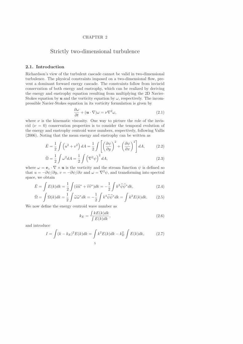
2.1. Introduction

Richardson’s view of the turbulent cascade cannot be valid in two-dimensionalturbulence. The physical constraints imposed on a two-dimensional flow, pre-vent a dominant forward energy cascade. The constraints follow from inviscidconservation of both energy and enstrophy, which can be realized by derivingthe energy and enstrophy equation resulting from multiplying the 2D Navier-Stokes equation by u and the vorticity equation by ω, respectively. The incom-pressible Navier-Stokes equation in its vorticity formulation is given by

∂ω

∂t+ (u · ∇)ω = ν∇2ω, (2.1)

where ν is the kinematic viscosity. One way to picture the role of the invis-cid (ν = 0) conservation properties is to consider the temporal evolution ofthe energy and enstrophy centroid wave numbers, respectively, following Vallis(2006). Noting that the mean energy and enstrophy can be written as

E =1

2

∫ (u2 + v2

)dA =

1

2

∫ [(∂ψ

∂y

)2

+

(∂ψ

∂x

)2]dA, (2.2)

Ω =1

2

∫ω2dA =

1

2

∫ (∇2ψ

)2

dA, (2.3)

where ω = ez · ∇ × u is the vorticity and the stream function ψ is defined sothat u = −∂ψ/∂y, v = −∂ψ/∂x and ω = ∇2ψ, and transforming into spectralspace, we obtain

E =

∫E(k)dk =

1

2

∫(uu∗ + vv∗)dk = −1

2

∫k2ψψ∗dk, (2.4)

Ω =

∫Ω(k)dk =

1

2

∫ωω∗dk = −1

2

∫k4ψψ∗dk =

∫k2E(k)dk. (2.5)

We now define the energy centroid wave number as

kE =

∫kE(k)dk∫E(k)dk

, (2.6)

and introduce

I =

∫(k − kE)2E(k)dk =

∫k2E(k)dk − k2

E

∫E(k)dk, (2.7)

5

6 2. STRICTLY TWO-DIMENSIONAL TURBULENCE

which upon temporal differentiation gives a measure of the spreading of theenergy distribution. To obtain (2.7), the definition of kE (2.6) has been used.If all energy is initially centred at kE , dI/dt should be larger than zero. Sinceboth energy and enstrophy are inviscidly conserved, it follows that

dkEdt

= − 1

2kEE

dI

dt< 0, (2.8)

(2.9)

which is consistent with an inverse energy cascade, i.e., a transfer of energytowards larger scales. Similarly, if we introduce an enstrophy wave numbercentroid kΩ and let

kΩ =

∫Ω(k)dk∫

k−1Ω(k)dk, (2.10)

and introduce

J =

∫(k−1 − k−1

Ω )2Ω(k)dk =

∫E(k)dk − k−2

Ω

∫Ω(k)dk, (2.11)

a little manipulation yields

dkΩ

dt=k3Ω

2Ω

dJ

dt> 0. (2.12)

Thus, the enstrophy wave number centroid (in which all enstrophy is initiallylocated) moves towards higher wave numbers (smaller scales) with time, whichcan be interpreted as a forward cascade of enstrophy. These are heuristic argu-ments but nevertheless show the general tendency for the cascade directions.Note that this argument does not forbid energy to be transferred to smallerscales, it just tells that more of the energy propagates towards larger scales.The same argument holds for the enstrophy cascade.

Our next step is to elaborate on the existence of a double cascade scenarioand inertial ranges in two-dimensional turbulence. Let us consider a case inwhich we feed a turbulent system with energy at a scale kf . Given that thegeneral picture of the cascade directions holds, as reflected by the time evolutionof wave number centroids, we would expect energy to propagate upscale andenstrophy to propagate downscale. If there is no large-scale drag imposedand we consider an infinitely large domain, we would expect an undisturbedenergy cascade towards larger scales. Simultaneously, we would expect anenstrophy cascade towards smaller scales, ultimately removed by small-scaleviscous dissipation. Given a large enough Reynolds number so that kf <<kmax, it is reasonable to expect that there would be a region, kf < k < kmax,practically undisturbed by viscous dissipation. Assume that we feed the systemwith energy at a rate ǫ and enstrophy at a rate η (the two are related byǫ = η/k2

f ). In the energy cascade range, the only parameters of practical

importance would be the energy density E(k), the energy injection rate ǫ andwave number k. Accordingly, we let E(k) ∼ ǫakb. Dimensional reasoning givesthat a = 2/3 and b = −5/3 so that E(k) ∼ ǫ2/3k−5/3. Similar argumentation

2.1. INTRODUCTION 7

Figure 2.1. Qualitative picture of the double cascade offorced two-dimensional turbulence. From Vallis (2006).

gives that E(k) ∼ η2/3k−3 in the forward enstrophy cascade range. Thesepredictions were introduced by Kraichnan (1967) and Leith (1968) and areillustrated in figure 2.1. Thus, for the inverse energy cascade range,

E(k) = Kǫ2/3k−5/3, (2.13)

and for the enstrophy cascade range;

E(k) = Cη2/3k−3, (2.14)

where we refer to C as the Kraichnan constant in forced two-dimensional turbu-lence and the Batchelor-Kraichnan constant in decaying two-dimensional tur-bulence (Batchelor, 1969). One major assumption that these predictions relyon is the locality of the cascades, meaning that it is assumed that there is nointeraction with scales outside the inertial ranges. Already in 1967, Kraichnanhypothesized that a logarithmic correction should manifest in the k−3 enstro-phy cascade range, although he did not provide any exact details on its form.In a follow-up paper, Kraichnan (1971), provided a complimentary theoreticalprediction, namely

E(k) = C′η2/3ω k−3

[ln

(k

k1

)]−1/3

, (2.15)

where C′ is a constant of order unity, which Kraichnan estimated to 2.626 basedon a turbulence test-field model and k1 marks the lowest wavenumber of theinertial range. The reason for this correction to the clean k−3-spectrum, is thatthe enstrophy flux would otherwise grow with k as a consequence of a diverging


rate of shear integral at low k ∼ k1. This correction allows for a k-independentC′ and a constant enstrophy flux range.

2.2. The enstrophy cascade

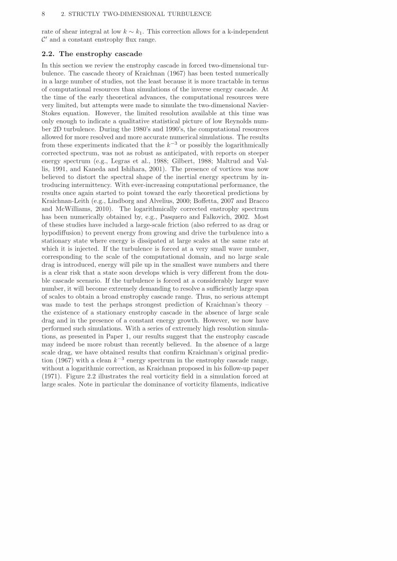
In this section we review the enstrophy cascade in forced two-dimensional tur-bulence. The cascade theory of Kraichnan (1967) has been tested numericallyin a large number of studies, not the least because it is more tractable in termsof computational resources than simulations of the inverse energy cascade. Atthe time of the early theoretical advances, the computational resources werevery limited, but attempts were made to simulate the two-dimensional Navier-Stokes equation. However, the limited resolution available at this time wasonly enough to indicate a qualitative statistical picture of low Reynolds num-ber 2D turbulence. During the 1980’s and 1990’s, the computational resourcesallowed for more resolved and more accurate numerical simulations. The resultsfrom these experiments indicated that the k−3 or possibly the logarithmicallycorrected spectrum, was not as robust as anticipated, with reports on steeperenergy spectrum (e.g., Legras et al., 1988; Gilbert, 1988; Maltrud and Val-lis, 1991, and Kaneda and Ishihara, 2001). The presence of vortices was nowbelieved to distort the spectral shape of the inertial energy spectrum by in-troducing intermittency. With ever-increasing computational performance, theresults once again started to point toward the early theoretical predictions byKraichnan-Leith (e.g., Lindborg and Alvelius, 2000; Boffetta, 2007 and Braccoand McWilliams, 2010). The logarithmically corrected enstrophy spectrumhas been numerically obtained by, e.g., Pasquero and Falkovich, 2002. Mostof these studies have included a large-scale friction (also referred to as drag orhypodiffusion) to prevent energy from growing and drive the turbulence into astationary state where energy is dissipated at large scales at the same rate atwhich it is injected. If the turbulence is forced at a very small wave number,corresponding to the scale of the computational domain, and no large scaledrag is introduced, energy will pile up in the smallest wave numbers and thereis a clear risk that a state soon develops which is very different from the dou-ble cascade scenario. If the turbulence is forced at a considerably larger wavenumber, it will become extremely demanding to resolve a sufficiently large spanof scales to obtain a broad enstrophy cascade range. Thus, no serious attemptwas made to test the perhaps strongest prediction of Kraichnan’s theory –the existence of a stationary enstrophy cascade in the absence of large scaledrag and in the presence of a constant energy growth. However, we now haveperformed such simulations. With a series of extremely high resolution simula-tions, as presented in Paper 1, our results suggest that the enstrophy cascademay indeed be more robust than recently believed. In the absence of a largescale drag, we have obtained results that confirm Kraichnan’s original predic-tion (1967) with a clean k−3 energy spectrum in the enstrophy cascade range,without a logarithmic correction, as Kraichnan proposed in his follow-up paper(1971). Figure 2.2 illustrates the real vorticity field in a simulation forced atlarge scales. Note in particular the dominance of vorticity filaments, indicative

2.2. THE ENSTROPHY CASCADE 9

Figure 2.2. Vorticity field and zoom in from a simulationforced at large scales, showing the dominance of vorticity fila-ments, resulting from a forward enstrophy cascade.

100

101

102

10310

−1

100

101

N8192LN16384LH16384L

k3E

(k)ǫ

−2/3

ω

k/kf

Figure 2.3. Compensated energy spectra, k3E(k)ǫ−2/3ω , from

a set of very high resolution simulations of forced two-dimensional turbulence.

of the forward enstrophy cascade. This cascade dominates the dynamics atseveral wave number decades, as shown in figure 2.3. However, the universalitymight fail with the constant C, which has been found to vary in our simulations.


2.3. The energy cascade

A stationary inverse energy cascade range can only be obtained in the presenceof a large scale drag, since energy would otherwise cascade indefinitely towardslarger scales. In reality, there is a physical limit on how far the cascade canreach, namely the domain size. As energy reaches the smallest wave number, itwill continuously pile up at this wave number, forming what is referred to as anEinstein-Bose condensate. Such a condensate can clearly bring the system awayfrom the double cascade scenario by Kraichnan-Leith (e.g., Smith and Yakhot,1994). In order to generate a double cascade with two wide inertial ranges,very high resolution simulations are required. Boffetta (2007) performed suchsimulations, showing a nearly perfect k−5/3 inverse cascade range in presenceof a linear Ekman drag, while obtaining an enstrophy inertial range a littlesteeper than k−3, mainly for the highest resolution simulations. A linear dragis often introduced as a large-scale energy dissipation mechanism, found in realsystems such as the atmosphere and in physical experiments. By investigatingthe fluxes of energy and enstrophy in physical space, Boffetta (2007) foundthat there is a very small correlation between the fluxes of these. This suggeststhat it should be possible to generate a single cascade of energy. This was alsoproposed by Tran and Bowman (2004). Therefore, it seems possible to force thefluid at scales near the small-scale dissipation range and obtain the classicalk−5/3-spectra, despite dissipating nearly all enstrophy at the forcing scales.However, this suggestion has been cast in doubt. Starting with Borue (1994),it was found that the implementation of a large-scale hypodiffusion steepensthe energy spectrum considerably to almost a k−3-spectrum. The possiblereason was found in the presence of vortices over all scales, whereas Boffetta etal. (2000) explained it in terms of a bottleneck effect as in three-dimensionalturbulence (Falkovich, 1994). However, Smith and Yakhot (1994) found thatthe k−5/3-spectrum steepened to an exponent . −2 when resolving both ofthe cascades, as a consequence of vortex generation in the enstrophy cascaderange. This result was later confirmed by Scott (2007), who provided estimateson when this steepening occurs by comparing the forcing wave number with thehighest resolved wavenumber, based on high resolution simulations. A closerlook at the results by Boffetta indicates that there is a small range located nearthe forcing scale in the inverse cascade, exhibiting a steeper slope than −5/3.To summarize, the issue seems rather involved, and there is no clear evidencefor a universal and local energy inertial range, as also highlighted by Danilovand Gurarie (2001a, 2001b). As a response to these differing results, we haveperformed a set of high resolution simulations with and without a large scalelinear drag of varying strength and with a variable forcing wave number. It hasbeen found that the form of the energy spectrum is sensitive to the strengthof the large scale drag. With the introduction of an infrared Reynolds numberReα = kf/kα, where kf is the forcing wave number and kα is a frictional wave

number, we demonstrate in paper 3 that the k−5/3 energy spectrum steepensto k−2 or steeper at high Reα.

2.4. DECAYING TURBULENCE 11

2.4. Decaying turbulence

Decaying turbulence describes the evolution of a flow field in the absence offorcing and without any large scale dissipation, principally conserving energy athigh Reynolds number. In that sense, decaying turbulence might be consideredthe purest case of two-dimensional turbulence. However, the initial conditionsmay differ considerably, although this should not cause any different resultsif the evolution is to be universal as predicted by Kraichnan-Batchelor-Leith.Therefore, it would seem natural that this case should be subject to less dispute.This is not the case. In fact, decaying 2D turbulence has been subject torenewed interest. As an initial flow field is released to decay freely, we couldexpect energy to cascade toward larger scales, where it is unaffected by small-scale viscosity, and so conserving energy, whereas the enstrophy would cascadetoward smaller scales where it is dissipated. The question is how the energyspectrum evolves under these circumstances? According to Batchelor (1969),we could anticipate the survival of an enstrophy cascade, with an enstrophy

spectrum scaling as Ω(k) ∼ ǫ2/3ω k−1, where ǫω is the enstrophy dissipation

rate. This is the classical scenario. However, Dritschel et al. (2007) questionedthis theoretical prediction. According to Dritschel et al. (2007), the enstrophydissipation vanishes in the limit ν → 0 and this suggests that the enstrophyspectrum should instead scale as Ω(k) ∼ Ωk−1(lnRe)−1. However, we haveperformed a number of very high resolution simulations (as presented in paper2) in which we find that Dritschel’s argument that the inertial range shouldcontain an increasing portion of the total enstrophy with time should be calledinto question. Thus, the relative enstrophy content has been found to increaseat the lower wave number end, where a number of coherent vortices reside.Our simulations also show that the Batchelor-Kraichnan constant C is of orderunity, but varies, possibly as a consequence of extreme intermittency in theenstrophy dissipation, thus following the argument by Landau and Lifshitz(1987). In essence, we reproduced Batchelor’s result, with a k−1 enstrophyspectrum in all our simulations, despite very different initial conditions, whichare visible also at later times (see figure 2.4). Our results are illustrated infigure 2.5, which shows the compensated enstrophy spectra kΦ(k)χ−2/3, whereΦ(k) is the enstrophy spectrum and χ is the enstrophy dissipation rate, fromthree simulations with different initial conditions, taken at three instances intime. It is noteworthy that the steeper spectra obtained by earlier investigators(e.g., McWilliams, 1984 and Bartello and Warn, 1996), might be an artefactof a low Reynolds number, since the width of the enstrophy inertial range

decreases slowly with time as the dissipation wave number kd ∼ ǫ1/6ω ν

−1/2ω , and

ǫω decreases with time. We have also found that power law exponents of decayrates of quantities such as the enstrophy and hence enstrophy dissipation aredependent on the initial conditions. This has been shown also by van Bokhovenet al. (2007).


Figure 2.4. Snapshots of the ”final” states from three sim-ulations of decaying two-dimensional turbulence with variousinitial conditions. Red colour corresponds to positive vorticityand blue colour to negative vorticity.

10−3

10−2

10−1

100

10−4

10−2

100

k Φ

(k)

/ χ2/

3

k ηω

Figure 2.5. Compensated enstrophy spectra from three sim-ulations (red, blue and green) of decaying two-dimensionalturbulence, taken at three instances (solid, dashed and dot-ted) during each simulation. The abscissa is a nondimensionalwavenumber, where ηω = ν1/2χ−1/6 is a characteristic scale ofenstrophy dissipation.

2.5. Coherent structures

We have performed a number of simulations revealing the existence of strongand long-lived vortices which we refer to as coherent structures. They are easyto distinguish by the human eye as they stand out as ordered structures ina chaotic sea of filamentary vorticity debris (see figure 2.4). They are alsobelived to cause departures from universal scaling laws in two-dimensional tur-bulence. McWilliams (1984, 1990) found early evidence of stuctures containinga substantial fraction of vorticity of two-dimensional flows, with lifetimes farexceeding the characteristic time for nonlinear interactions. He found that vor-tices spontaneously develop if the forcing and friction is relatively weak and theReynolds number sufficiently high. They are approximately axisymmetric and

2.6. β-PLANE TURBULENCE 13

are stable to perturbations from the quiescent surroundings but not to encoun-ters by other strong vortices, which could result in like-sign vortex mergers.McWilliams (1990) noted that the lock-up of vorticity inside coherent vorticeseffectively reduces cascade rates of both enstrophy and energy. By introducinga vortex-census algorithm, he enabled detailed studies of their properties andfound a general trend of the ”survival of the fittest”. Dritschel (1995) con-tributed with a detailed study of vortex interactions and showed that theseare relatively short inelastic interactions resulting in two or three new coherentvortices, thus questioning the picture of the inverse energy cascade as a se-ries of merging events resulting in ever-growing vortices, as suggested by, e.g.,Borue (1994), in forced two-dimensional turbulence. In decaying turbulence, itis more evident that large-scale structures form as a result of vortex mergers,finally resulting in two opposite-sign vortices (Tabeling, 2002). An interest-ing question is whether any universal theory can account for coherent vortices.Carnevale et al. (1991) suggested such a theory for vortex circulation, radius,mean enstrophy and kurtosis, but there are ample examples of deviations fromsuch a governing theory (Tabeling, 2002).

2.6. β-plane turbulence

To accomodate for a background rotation, a β-plane approximation has beenintroduced to the 2D Navier-Stokes equation;

∂ω

∂t+ (u · ∇)ω = −ν∇2ω − βv. (2.16)

The β-term arises from the following argument. We consider a rotating spheresuch as illustrated in figure 2.6. and note that the Coriolis force 2Ω × u canbe rewritten by defining

f ≡ 2Ω sinφez, (2.17)

where ez is the normal unit vector to a locally Cartesian tangent plane on thesphere. For small variations in the meridional direction

f = 2Ω sinφ ≃ 2Ω sinφ0 + 2Ω(φ− φ0) cosφ0, (2.18)

and we approximate the Coriolis parameter to vary linearly on the tangentplane as

f = f0 + βy, (2.19)

wheref0 = 2Ω sinφ0. (2.20)

Thus

β =df

dy=

2Ωcosφ0

R⊕

, (2.21)

where R⊕ is the radius of the Earth, and equation (2.16) approximately de-scribes the motions on a rotating sphere, provided that the flow is spatiallylimited so that the geometric effects of sphericity are negligible, and is knownas the β-plane approximation. It allows for the use of a local Cartesian rep-resentation of the Navier-Stokes equation, while still capturing the important


dynamical effects stemming from sphericity and is dynamically equivalent to adifferentially rotating system.

We thus see the existence of an additional term βv on the right hand side.We may now ask what dynamical consequences the inclusion of this term mighthave. Rhines (1975) investigated this matter and showed that turbulent energyis dispersed into waves at scales larger than approximately

kβ =

√β

2√E, (2.22)

where E is the r.m.s. energy of the flow. This scale is approximate and thereexists a number of definitions of this arrest scale, which do not differ too much.Thus, the inverse energy cascade continues up to a scale kβ , from which noupscale energy cascade is possible. Instead, the transition to wave propaga-tion (Rossby waves) is overtaken by a flow characterized by steady alternatingzonal jets. This picture is helpful in explaining the characteristic size of eddiesin the Earth’s atmosphere, and the prevalence of zonal flows. The waves arereferred to as Rossby waves, and its dispersion relation can be obtained bylinearizing (2.16) upon a basic state with a perturbation. Rossby waves arean important ingredient in atmospheric dynamics, with large effects on bothdaily weather and regional climate. Many numerical experiments over the yearshave to a large degree verified Rhines’ prediction. Maltrud and Vallis (1991)found that the β-effect tend to destroy coherent vortices at large scales but thatthe resulting anisotropy at scales larger than kβ does not influence the inertialrange characteristics at smaller scales. Later studies have concerned the statis-tical characteristics of the resulting zonal jets (e.g., Vallis and Maltrud, 1993;Manfroi and Young, 1998; Danilov and Gurarie, 2004). It is noteworthy thatattempts have been made to explain the atmospheric flow structure on Jupiter,with its zonal jets and superstationary vortices, in terms of two-dimensional orquasigeostrophic turbulence with a β-effect (e.g., Kukharkin and Orszag, 1996;Smith, 2004). An example of a simulation with a β-effect is shown in figure 2.7(left), where the anisotropy at large scales is clearly visible. Figure 2.7 (right)also shows a satellite image of Jupiter, with the characteristic zonal flow andthe famous red spot visible as a coherent vortex in the southern hemisphere.

2.6. β-PLANE TURBULENCE 15

Figure 2.6. Tangent plane approximation to the quasi-spherical Earth. The rotation vector components in the planeare shown as well as the direction of the unit vectors.

Figure 2.7. Left: vorticity snapshot from a simulation withmoderate β. Right: satellite image of Jupiter’s atmosphere(from NOAA).

CHAPTER 3

Quasigeostrophic turbulence

So far, we have considered two-dimensional turbulence. In many natural sys-tems, such as the atmosphere, there is a vertical stratification. Horizontalvariations of the density introduces potential energy into the system, whichcan be released by the excitation of baroclinic motions. These motions aremanifested in the atmosphere by the development of cyclones and anticyclonesin the midlatitudes, largely responsible for the day-to-day weather we experi-ence. These systems are generally fully developed at scales ∼ 1000 km and canin part be studied within the framework of QG turbulence. The dynamics isdescribed by the QG potential vorticity equation, which is given by

∂q

∂t+ (uh · ∇h) q + βv = (−1)n+1νq∇2nq + f + (−1)p+1νu∇−2pq, (3.1)

where

q = ∇2ψ (3.2)

is the QG potential vorticity, ∆ is the three-dimensional Laplace operator inscaled coordinates, ψ is the stream function, uh = uex+vey = −∂yψex+∂xψey

is the horizontal velocity and ∇h is the horizontal gradient operator, νq is thehyperviscosity coefficient and νu is an optional hypofriction (p > 0) or Ek-man drag (p = 0) coefficent. For a complete derivation of this equation, seeappendix A. The most important property of this equation is the inviscid con-servation of potential vorticity. Note also that the quasigeostrophic motion isin the horizontal plane but that these motions generally vary in the vertical.This turbulent regime was theoretized by Charney (1971). By scaling the ver-tical coordinate by N/f , he argued that the flow field should obey a specialtype of isotropy, which has been given the name Charney isotropy, after Char-ney (1971). Charney isotropy means that the energy spectrum, in the scaledvariables, is invariant in the different directions (e.g., horizontal and vertical).Charney also predicted approximate equipartition between kinetic and poten-tial energy in the three-dimensional energy spectra. The prediction of Charneyisotropy has been supported by numerical experiments such as Hua and Haid-vogel (1986) and McWilliams (1989).

Just as in two-dimensional turbulence, there is rich dynamics in the flow(see figure 3.1), with the development of coherent structures under favourableconditions. The presence of a vertical dimension introduces new features ofthese vortices, which can be barotropic or baroclinic to various degrees, and

16

3. QUASIGEOSTROPHIC TURBULENCE 17

Figure 3.1. Potential vorticity snapshot from a freely de-caying quasigeostrophic simulation. Red (blue) colour corre-sponds to positive (negative) potential vorticity.

for a thorough review of their statistical properties, it is recommended to con-sult, e.g., McWilliams (1990), McWilliams et al. (1999), von Hardenberg et al.(2000) and Reinaud et al. (2003). In paper 4, we present results on a seriesof high resolution simulations that essentially confirm Charney’s predictionsunder a wide range of conditions and the similarities with 2D turbulence. Fur-thermore, it is shown that the prediction might even be stronger than Charneyanticipated, since the general picture holds qualitatively also in presence of aplanetary vorticity gradient. It is also suggested in appendix A, that there isthe potential of extending the quasigeostrophic regime to scales approximatelyequal to the deformation radius.

CHAPTER 4

Numerical method and the codes

Two pseudospectral codes, PNSE2D and QGE3D have been developed to solve thetwo-dimensional Navier-Stokes and Charney QG potential vorticity equation,respectively. The codes have been written in Fortran90. Pseudospectral meansthat the time-stepping is performed in spectral space whereas the nonlinearproducts are calculated in real space. Fourier transforms are calculated with theaid of an efficient FFT-package called FFTW. Time-stepping is performed with aRunge-Kutta fourth order scheme and the time step is determined using a CFL-condition. Viscosity, being it small scale Navier-Stokes viscosity, hyperviscosityor large scale hypodiffusion or linear Ekman drag, is calculated with the useof an integrating factor technique. The codes are essentially free from aliasingerrors by the use of an 8/9-dealiasing technique, which allows for a wider rangeof Fourier modes to be captured compared to the traditional 2/3-dealiasing. Fora more thourough review of the details of the codes, see paper 5, which alsodiscusses some statistical measures and parallelisation approaches. It shouldbe noted that the codes have been customized to run on massively parallelsuper computers, to allow for very high resolution simulations. A survey of thespeedup of the codes is also presented in paper 5.

18

CHAPTER 5

Summary of the papers

Paper 1

The enstrophy cascade in forced two-dimensional turbulence. This paper inves-tigates the enstrophy cascade in forced two-dimensional turbulence by perform-ing a set of high resolution simulations with different forcing wave numbers.One of the simulations is larger than any other simulation presented in theliterature so far. In the absence of a large-scale drag, we obtain Kraichnan’soriginal prediction (1967) of a clean k−3 energy spectrum in the enstrophy in-ertial range. However, it is found that the Kraichnan constant varies slightlybetween the simulations and is decreasing very slowly with time. When forc-ing is applied at relatively large wave number, we obtain coherent vortices atscales larger than the forcing scale, and intermittency measures become verylarge at all scales. However, when forcing is applied at small wave number,intermittency statistics are close to Gaussian. The main conclusion is that theenstrophy cascade is a robust feature of two-dimensional turbulence.

Paper 2

Testing Batchelor’s similarity hypothesis for decaying two-dimensional turbu-

lence. This paper studies the enstrophy cascade in decaying two-dimensionalturbulence to test Batchelor’s hypothesis of an equilibrium range. By perform-ing three simulations with very different initial conditions, Batchelor’s hypoth-esis is corroborated. As in paper 1, it is found that the Batchelor-Kraichnanconstant varies. It is ∼1.4 in two of the simulations and ∼1.1 in one. It ishypothesized that a higher degree of intermittency of dissipation causes theconstant to be lower in one of the simulations.

Paper 3

Infrared Reynold’s number dependency of the two-dimensional inverse energy

cascade. In this paper, the inverse energy cascade is subject to high resolutionnumerical experiments. A surprising result is found, showing that the k−5/3-scaling in the inertial energy range is likely to be a low frictional Reynoldsnumber effect, in presence of a large-scale linear friction. When the inertialenergy range is wide enough, the linear friction is too weak at the forcing scalesto prevent the formation of coherent vortices. These act to steepen the energy

19

20 5. SUMMARY OF THE PAPERS

spectrum from k−5/3 to k−2 or steeper. The linear friction is shown to imposea larger effect than the ultraviolet dissipation.

Paper 4

Charney isotropy and equipartition in quasigeostrophic turbulence. This paperis devoted to studies of quasigeostrophic turbulence, as theoretized by Charney(1971). We verify Charney’s predictions of isotropy and equipartition by per-forming high resolution three-dimensional simulations. It is also demonstratedthat Charney’s predictions also holds in the presence of a β-effect and in freelydecaying quasigeostrophic turbulence. The analogy with two-dimensional tur-bulence is investigated and confirmed.

Paper 5

Simulations of two-dimensional and quasigeostrophic turbulence: Technical Re-

port. Paper 5 is a technical report that describes the two codes in greaterdetail. The code structures are explored and underlying assumptions, statisti-cal measures and code performance are presented for each code, respectively.The codes are found to scale well in massively parallel systems and they allowfor cutting edge numerical experiments.

CHAPTER 6

Outlook

It has become clear that Kraichnan’s and Batchelor’s predictions on the formof the energy spectrum in the enstrophy inertial range are robust at high Rey-nolds number. Earlier investigations found steeper energy spectrum and it wasbelieved to be an effect of intermittency. Our results suggest that intermit-tency only affects the Batchelor-Kraichnan constant and not the k−3-scaling.We now believe we are in a position to interpret this fact as a consequenceof intermittency in the enstrophy dissipation. This was originally addressedby Landau and Lifshitz (1987), who concluded that the spatial variance of thedissipation is nonuniversal and could thus not result in a universal averagingof the dissipation. Kraichnan (1974) elaborated on this argument, and con-cluded that this is a result of spatial averaging over the domain scale, whichcontains patches of enhanced dissipation larger than the inertial scales, whichwe aim to describe. Thus, when determining the dissipation rates, it shouldbe taken as an ensemble average of smaller subdomains making up the whole

flow field, since the average ǫω =< ǫ2/3ω > is different from ǫω

2/3. In paper 2,we suggest that the small variation observed in the constant may be explainedas a consequence of intermittency. In a revision of paper 1, this hypothesiswill be quantitatively investigated. Perhaps of greater physical interest, is toextend the quasigeostrophic framework to the primitive equations, which area set of nonlinear equations used in atmospheric and oceanic modeling (Vallis,2006). The equation set contains the momentum equations in the horizontal,the hydrostatic approximation in the vertical and is completed by the thermo-dynamic and continuity equations. The use of the primitive equations allowsfor variations of the Rossby deformation radius by varying the stratification,which is fixed in the framework of Charney quasigeostropy. By doing this, weaim to explore the dynamic origins of the atmospheric energy spectrum anddetermine the origin of the high wave number k−5/3-range.

21

Acknowledgements

First of all I would like to thank my supervisor Dr. Erik Lindborg for all hishelp and patience during the past three years. It has been a long and en-joyable journey, with many good laughs but also a scientific adventure withmany unexpected outcomes. I would also like to thank my co-advisor GeertBrethouwer for his help with getting me started in the implementation of thecodes. A great thank you also to Philipp Schlatter, who has given me goodadvices in order to increase the performance of the codes. The working envi-ronment has been very pleasant thanks to both a good atmosphere but alsothanks to the students in Dan Henningson’s group and Andreas Carlson, mycurrent office colleagues Amin Rasam and Enrico Deusebio, but also formerroomies Niklas Mellgren and Seif Dalilsafaei. The list would not be completewithout a thank you to my colleagues at the Swedish Television, in particularPar Holmgren and Helen Johansson, who have enabled me to stay in touchwith the real world of meteorology and climate. Something which also JennyBrandefelt have made possible. Thanks also to Johan Liakka at StockholmUniversity, whom I have shared thoughts and ideas with every now and then.I would also like to gratefully acknowledge the Linne FLOW centre, financedby the Swedish Research Council (Vetenskapsradet), for funding of the project.SNIC (Swedish National Infrastructure for Computing) is acknowledged forcomputer time at the Centre for Parallel Computers (PDC) at the Royal In-stitute of Technology in Stockholm and the National Supercomputer Centre(NSC) in Linkoping, with a generous grant by the Knut and Alice Wallenberg(KAW) foundation. Last, but not the least, I would like to thank Liisa for herlove, patience and encouragement.

22

APPENDIX A

Derivation of the QG potential vorticity equation

A.1. Introduction

This appendix gives an introduction to the dynamics of the midlatitude tro-posphere and more specifically the quasigeostrophic equations. These are aspecific set of equations that describes the synoptic scale motions in a boundeddomain on a rotating sphere such as the Earth. The aim is to derive a relevantformulation of the quasigeostrophic potential vorticity equation. The startingpoint will be the 3D Navier-Stokes equation on a rotating sphere, from whichwe will systematically exploit the involved terms on our way to quasigeostrophyfollowing Pedlosky (1987).

A.2. Scaling the 3D Navier-Stokes equation

We consider motions on a rotating sphere of radius r0, ignoring the slightdeparture from sphericity of the Earth. We assume that the vertical scale ofmotion is small enough so that the gravitational acceleration can be consideredconstant through the depth of the fluid. In addition, we assume that the scalesare large enough so that viscous effects can be ignored. Since we can anticipatethat the geostrophic approximation must fail near the equator, the theory mustapply to a spatial extent that is less than global. Hence, the restriction is that

O(Lr0

)< 1. The spherical coordinate system is defined in such a way that the

radius r defines the surface-normal direction, whereas θ is the latitude and φ isthe longitude. Neglecting viscous effects, friction and forcing, the momentumand mass continuity equations are given by

Du

Dt+ 2Ω × u = −1

ρ∇p+ g, (A.1)

Dρ

Dt+ ρ∇ · u = 0, (A.2)

D

Dt≡ ∂

∂t+ u · ∇. (A.3)

In spherical coordinates, the mass continuity equation can be expressed as

Dρ

Dt+ ρ

[1

r2∂(r2w)

∂r+

1

r cos θ

∂(v cos θ)

∂θ+

1

r cos θ

∂u

∂φ

]= 0, (A.4)

23

24 A. DERIVATION OF THE QG POTENTIAL VORTICITY EQUATION

D

Dt=

∂

∂t+

u

r cos θ

∂

∂φ+v

r

∂

∂θ+ w

∂

∂r. (A.5)

Now let

u = uφ + vθ + wr, (A.6)

u ≡ r cos θDφ

Dt, (A.7)

v ≡ rDθ

Dt, (A.8)

w ≡ Dr

Dt. (A.9)

Hence,

Du

Dt= φ

Du

Dt+ θ

Dv

Dt+ r

Dw

Dt+ u

Dφ

Dt+ v

Dθ

Dt+ w

Dr

Dt. (A.10)

Similarity consideration shows that

limδx→0

|δφ|δx

=1

r cos θ, (A.11)

δφ

δx=

1

r cos θ

(θ sin θ − r cos θ

), (A.12)

Dφ

Dt=

u

r cos θ

(θ sin θ − r cos θ

), (A.13)

and equivalently for the θ and r unit vectors it can be shown that

Dθ

Dt= −u tan θ

rφ − v

rr, (A.14)

Dr

Dt=u

rφ +

v

rθ. (A.15)

Thus, the acceleration following the relative motion in spherical coordinates isgiven by

Du

Dt= φ

(Du

Dt− uv tan θ

r+uw

r

)+θ

(Dv

Dt+u2 tan θ

r+vw

r

)+r

(Dw

Dt− u2 + v2

r

).

(A.16)Expansion of the Coriolis term in spherical coordinates is now demonstratedbelow;

2Ω×u = 2Ω

∣∣∣∣∣∣∣

φ θ r

0 cos θ sin θu v w

∣∣∣∣∣∣∣= 2Ω

[(w cos θ − v sin θ) φ + u sin θθ − u cos θr

].

(A.17)

A.2. SCALING THE 3D NAVIER-STOKES EQUATION 25

The pressure gradient and gravity are trivially expressed and can easily beidentified in the component form of (A.1), as shown below:

Du

Dt+uw

r− uv

rtan θ + 2Ωw cos θ − 2Ωv sin θ = − 1

ρr cos θ

∂p

∂φ, (A.18)

Dv

Dt+vw

r+u2

rtan θ + 2Ωu sin θ = − 1

ρr

∂p

∂θ, (A.19)

Dw

Dt− u2 + v2

r− 2Ωu cos θ = −1

ρ

∂p

∂r− g. (A.20)

The momentum and mass continuity equation need to be complemented by thethermodynamic equation;

Dθ

Dt=

θ

cpT

(k

ρ∇2T +Q

), (A.21)

where k is the thermal conductivity, T the temperature, Q the rate of heat ad-dition per unit mass by internal heat sources and θ is the potential temperature,defined as

θ = T

(p0

p

) Rcp

. (A.22)

Note that p, ρ and T are related by the ideal gas law;

p = ρRT. (A.23)

Now, we consider motions, whose horizontal spatial scale of variation is givenby the length scale L and velocity scale U . Furthermore, we restrict ourselves tothe mid-latitude region centred at around some latitude θ0. In addition, we re-strict ourselves to Cartesian coordinates by replacing the spherical coordinatesas follows

x = φr0 cos θ0,y = r0(θ − θ0),

(A.24)

and hence ∂∂φ = r0 cos θ0

∂∂x ,

∂∂θ = r0

∂∂y .

(A.25)

In addition, the following substitutions are introduced

z = r − r0 = Dz′,x = Lx′,y = Ly′,t = L

U t′,

u = Uu′,v = Uv′,w = D

LUw′.

(A.26)

Note that the time scales advectively. We now turn to the hydrostatic approx-imation;

∂ps∂z

= −ρs(z)g, (A.27)


where the subscript s denotes a standard basic state upon which perturbationsoccur such that

p = ps(z) + p(x, y, z, t),ρ = ρs(z) + ρ(x, y, z, t).

(A.28)

We need to scale the pressure and density pertubations in some sense. Itcan be conjectured that for the motions of interest, the horizontal pressuregradient will be of the same order of magnitude as the Coriolis acceleration,

i.e., O(ρs2Ωu sin θ0) ∼ O(pL

)→ p ∼ O(ρsUf0L), where

f0 = 2Ω sin θ0, (A.29)

is the Coriolis parameter at θ0. Hence,

p = ps(z) + ρs(z)Uf0Lp′. (A.30)

In a similar manner, we may anticipate that the buoyancy force due to ρ willbe of the same order of magnitude as the vertical pressure gradient by recalling

the hydrostatic approximation, upon which ∂p∂z = O

(pD

)= O

(ρsUf0LD

)∼

O(ρg) → O(ρ) = O(ρsU

f0LgD

). Hence, we may write

ρ = ρs(z)[1 +Ro Fρ′

], (A.31)

where Ro ≡ U

f0L≡ ǫ,

F =f2

0L2

gD .(A.32)

Here, Ro = ǫ is the Rossby number. We are now at the point where the mo-mentum equation components can be non-dimensionalized following the substi-tutions addressed so far. Thus, applying (A.26), (A.27), (A.30) and (A.31) tothe component momentum equations and dividing through by Uf0, we obtain

ǫ

[Du′

Dt′+L

r∗

(δu′w′ − u′v′ tan θ

)]− v′

sin θ

sin θ0+ δw′ cos θ

sin θ0=

= −r0r∗

cos θ0cos θ

1

1 + ǫFρ′∂p′

∂x′, (A.33)

ǫ

[Dv′

Dt′+L

r∗

(δv′w′ + u′2 tan θ

)]+ u′

sin θ

sin θ0= −r0

r∗

1

1 + ǫFρ′∂p′

∂y′, (A.34)

D(1 + ǫFρ′)

U2

(D

L2

Dw′

Dt′− u′2 + v′2

r∗

)− 2ΩUu′ cos θ

=

= − 1

ρs

∂

∂z′[ps + Uf0Lρsp

′]−D(1 + ǫFρ′)g∗, (A.35)

where the subscript ∗ denotes dimensional quantities and

δ ≡ D

L. (A.36)

A.2. SCALING THE 3D NAVIER-STOKES EQUATION 27

The vertical component (A.35) can be further simplified by expansion of theright hand side to yield, after division by Uf0L;

(1 + ǫFρ′)

[ǫδ2

Dw′

Dt′− ǫδL

r∗(u′2 + v′2) − δu′

cos θ

sin θ0

]= − 1

ρs

∂

∂z′(ρsp

′) − ρ′.

(A.37)The nondimenzionalized total derivative takes the following form

D

Dt′=

∂

∂t′+ u′

r0r∗

cos θ0cos θ

∂

∂x′+ v′

r0r∗

∂

∂y′+ w′ ∂

∂z′. (A.38)

Note thatr∗r0

= 1 + δ

(L

r0

)z′. (A.39)

Expanding the mass continuity equation (A.4) and applying the substitutionsresult in the nondimensional version

ǫFDρ′

Dt′+ (1 + ǫFρ′)

[w′

ρs

∂ρs∂z′

+∂w′

∂z′+ 2

D

r∗w′ +

r0r∗

∂v′

∂y′+

− L

r∗v′ tan θ +

r0r∗

cos θ0cos θ

∂u′

∂x′

]= 0. (A.40)

In the following, the superscripts ′ denoting the nondimensional variables will bedropped and the subscript ∗ will denote dimensional remnants in the equations.It is important to note that no restrictive approximations have been appliedso far. The equations have just been scaled so that their relative magnitudecan be estimated by the nondimensional parameters multiplying the individualterms. Before investigating any specific parameter settings, we expand thetrigonometric terms around the θ0-latitude in Taylor expansions, i.e.,

sin θ = sin θ0 +d(sin θ)

dθ|θ=θ0(θ − θ0) +

d2(sin θ)

dθ2|θ=θ0

(θ − θ0)2

2!+ ... (A.41)

With the use of (A.24) and (A.26) we thus obtain

sin θ = sin θ0 + Lr0y cos θ0 − 1

2

(Lr0

)2

y2 sin θ0 + ... ,

cos θ = cos θ0 − Lr0y sin θ0 − 1

2

(Lr0

)2

y2 cos θ0 + ... ,

tan θ = tan θ0 + Lr0y 1

cos2 θ0+(Lr0

)2

y2 tan θ0cos2 θ0

+ ... ,

(A.42)

Last, but not the least, we now define the β-parameter as

β0 =d

dy(2Ω sin θ) |θ=θ0 =

1

r0

d

dθ(2Ω sin θ) |θ=θ0 =

2Ω

r0cos θ0 (A.43)

It can be noted here that β0Lf0

= ... = Lr0

cot θ0 ∼ O(Lr0

)and hence β0L

f0=

β0L2

U ∼ O(Lǫr0

)so that the magnitude of the relative vorticity- to the planetary


vorticity gradient is measured by

1

β=

U

β0L2∼ O

(ǫr0L

), (A.44)

which is evidentally determined by the relative size of the Rossby number andthe inverse ratio between the horizontal length scale and approximately theEarth’s radius for tropospheric considerations.

A.3. The geostrophic approximation

So far, no specific scale of motion has been chosen. By noting that in themidlatitude atmosphere,

U ∼ O(10 ms−1),L ∼ O(1000 km),D ∼ O(10 km),f0 ∼ O(10−4 s−1) ,

(A.45)

we first choose to study the case ǫ ∼ O(Lr0<< 1

), i.e., motions that are

less than global. Under these circumstances, Uβ0L2 ∼ O

(10

10−11(106)2

)∼ O(1).

Thus, the planetary vorticity gradient is expected to play an active role in theatmospheric dynamics at this horizontal length scale. Making use of (A.45),we can summarize the key parameters as

ǫ ∼ O(10−1),β ∼ O(1),

F =f2

0L2

gD ∼ O(10−1) ∼ O(ǫ),Lr0

∼ O(ǫ),

δ = DL ∼ O(10−2) ∼ O(ǫ2),

r∗r0

− 1 ∼ O(δ Lr0

)∼ O(ǫ3),

(A.46)

The limit ǫ → 0, ǫr0L ∼ O(1), is a special case that examines geostrophic dy-namics when the planetary vorticity gradient contributes equally to the relativevorticity gradient. We now express all the dynamic variables, i.e., u, v, w, p, ρ,in series of the key parameter ǫ such that

u(x, y, z, t) = u0(x, y, z, t) + ǫu1(x, y, z, t) + ǫ2u2(x, y, z, t) + ... etc. (A.47)

A.3. THE GEOSTROPHIC APPROXIMATION 29

Applying (A.42), (A.46) and the first two terms of (A.47) for the dynamicvariables to (A.33), (A.34) and (A.37), we obtain

ǫ

[D(u0 + ǫu1)

Dt+L

r∗

(ǫ2(u0 + ǫu1)(w0 + ǫw1)+

− (u0 + ǫu1)(v0 + ǫv1)

(tan θ0 +

Ly

r0cos−2 θ0

))

+

− (v0 + ǫv1)

(sin θ0 + Ly

r0cos θ0

)

sin θ0+ ǫ(w0 + ǫw1)

(cos θ0 − Ly

r0sin θ0

)

sin θ0=

= −r0r∗

cos θ0(cos θ0 − Ly

r0sin θ0

) 1

1 + ǫ2(ρ0 + ǫρ1)

∂(p0 + ǫp1)

∂x, (A.48)

ǫ

[D(v0 + ǫv1)

Dt+L

r∗

(ǫ2(v0 + ǫv1)(w0 + ǫw1)+

+ (u0 + ǫu1)2

(tan θ0 +

Ly

r0cos−2 θ0

))

+ (u0 + ǫu1)

(sin θ0 + Ly

r0cos θ0

)

sin θ0=

= −r0r∗

1

1 + ǫ2(ρ0 + ǫρ1)

∂(p0 + ǫp1)

∂y, (A.49)

(1 + ǫ2(ρ0 + ǫρ1)

)[ǫ5D(w0 + ǫw1)

Dt− ǫ3L

r∗

((u0 + ǫu1)

2 + (v0 + ǫv1)2)

+

− ǫ2(u0 + ǫu1)

(cos θ0 − Ly

r0sin θ0

)

sin θ0

=

= − 1

ρs

∂

∂z

(ρs(p0 + ǫp1)

)− (ρ0 + ǫρ1), (A.50)

The mass continuity equation (A.40) takes the form

ǫ2D(ρ0 + ǫρ1)

Dt+(1 + ǫ2(ρ0 + ǫρ1)

)[w0 + ǫw1

ρs

∂ρs∂z

+∂(w0 + ǫw1)

∂z+

+2D

r∗(w0 + ǫw1) +

r0r∗

∂(v0 + ǫv1)

∂y− L

r∗(v0 + ǫv1)

(tan θ0 +

Ly

r0cos−2 θ0

)+

+r0r∗

cos θ0

cos θ0 − Lyr0

sin θ0

∂(u0 + ǫu1)

∂x

= 0. (A.51)


If we note that O(Dr∗

)< O(ǫ2), and establish that terms of like order in ǫ

must balance, we obtain, to first order,

v0 = ∂p0∂x ,

u0 = −∂p0∂y ,

ρ0 = − 1ρs

∂∂z (p0ρs) ,

1ρs

∂(w0ρs)∂z + ∂u0

∂x + ∂v0∂y = 0.

(A.52)

The equation set (A.52) is the geostrophic approximation. The O(1) motionis thus determined by the horizontal pressure gradient. Furthermore, it can beestablished that the O(1) geostrophic velocities are horizontally nondivergent,since

∂v0∂y

+∂u0

∂x= 0, (A.53)

which implies that

∂

∂z(ρsw0) = 0. (A.54)

Hence, ρsw0 is independent of z and if w0 = 0 for any z, it will be zero ∀z, e.g.,if the domain is bounded below or above. Thus, the vertical velocity is givenby

w(x, y, z, t) = ǫw1(x, y, z, t) + ǫ2w2(x, y, z, t) + ... (A.55)

which is a direct consequence of the geostrophic approximation. Therefore,we cannot determine p0 and hence u0 and v0 without considering higher orderdynamics. The O(ǫ) terms with the use of (A.55) are given below, startingwith the zonal component

Du0

Dt− Ly

ǫr0v0 cot θ0 − v1 = −∂p1

∂x− Ly

ǫr0tan θ0

∂p0

∂x, (A.56)

where the second term on the right hand side was obtained by a little manip-ulation;

− r0r∗

cos θ0

cos θ0 − Lyr0

sin θ0

∂p0

∂x=

= −r0r∗

cos θ0

(cos θ0 + Ly

r0sin θ0

)

(cos θ0 − Ly

r0sin θ0

)(cos θ0 + Ly

r0sin θ0

) ∂p0

∂x=

= −r0r∗

cos2 θ0 + Lyr0

cos θ0 sin θ0

cos2 θ0 −(Lr0

)2

y2 sin2 θ0

∂p0

∂x≈ L

r∗y tan θ0

∂p0

∂xQ.E.D. (A.57)

The meridional O(ǫ) component is given by

Dv0Dt

+ u0Ly

ǫr0cot θ0 + u1 = −∂p1

∂y. (A.58)

A.3. THE GEOSTROPHIC APPROXIMATION 31

The total derivative is given by

D

Dt=

∂

∂t+(u0+ǫu1)

r0r∗

cos θ0

cos θ0 − Lyr0

sin θ0

∂

∂x+(v0+ǫv1)

r0r∗

∂

∂y+ǫw1

∂

∂z, (A.59)

so that (A.56) and (A.58) become

∂u0

∂t + u0∂u0

∂x + v0∂u0

∂y − v1 − v0Lyǫr0

cot θ0 = −∂p1∂x − Ly

ǫr0tan θ0

∂p0∂x ,

∂v0∂t + u0

∂v0∂x + v0

∂v0∂y + u1 + u0

Lyǫr0

cot θ0 = −∂p1∂y .

(A.60)We complete with the mass continuity equation:

1

ρs

∂

∂z(ρsw1) +

∂u1

∂x+∂v1∂y

− v0L

ǫr0tan θ0 +

Ly

ǫr0tan θ0

∂u0

∂x= 0. (A.61)

Pedlosky (1987) discusses the presence of terms that are ∼ Lǫr0

in the momen-

tum equation (A.60), and notes that these terms on the left hand side are dueto the variation of the Coriolis parameter on a β-plane whereas on the righthand side, these terms reflect the variation of the metric term cos θ. If tan θ0would be small, this term would be negligible. Then (A.60) would reduce tothe O(ǫ) momentum equation for a flat Earth with a linearly varying Corioliosparameter in the meridional direction. However, this would push the domainto latitudes near the equator, where the theory fails. Thus, a model of a flatEarth with sphericity accounted for only by a varying f is not valid for theO(ǫ) momentum balance. Pedlosky (1987) states however, that the β-planeapproximation only requires that the vorticity equation satisfies the β-planeapproximation. By taking − ∂

∂y (A.60 a) + ∂∂x (A.60 b), and noting that the

relative vorticity is given by

ζ0 =∂v0∂x

− ∂u0

∂y, (A.62)

we yield after some simplification that

∂ζ0∂t

+ u0∂ζ0∂x

+ v0∂ζ0∂y

+

(∂u1

∂x+∂v1∂y

)+ v0

L

ǫr0cot θ0 =

=L

ǫr0tan θ0

∂p0

∂x+Ly

ǫr0tan θ0

∂2p0

∂x∂y, (A.63)

where use have been made of the nondivergence of the O(1)-momentum. Wecan simplify this further by taking advantage of the fact that

1

β=

U

β0L2=

Uf0r0L2 cot θ0

=

[L

r0∼ ǫ

]=

U

ǫf0L cot θ0=

[U

f0L∼ ǫ

]=

1

cot θ0,

(A.64)upon which we obtain

∂ζ0∂t

+u0∂ζ0∂x

+v0∂ζ0∂y

+βv0 =L

ǫr0

[tan θ0

∂p0

∂x+ y tan θ0

∂2p0

∂x∂y

]−(∂u1

∂x+∂v1∂y

).

(A.65)


From the geostrophic approximation (A.52), the mass continuity equation(A.61) can be rewritten as

1

ρs

∂(ρsw1

∂z+

(∂u1

∂x+∂v1∂y

)− L

ǫr0tan θ0

∂p0

∂x− Ly

ǫr0tan θ0

∂2p0

∂x∂y= 0, (A.66)

from which we clearly can rewrite (A.65) as

D0

Dt[ζ0 + βy] =

1

ρs

∂(ρsw1)

∂z, (A.67)

whereD0

Dt≡ ∂

∂t+ u0

∂

∂x+ v0

∂

∂y. (A.68)

It is now clear that (A.67) is the vorticity equation for a flat Earth model witha linearly varying Coriolis parameter in the meridional direction. The O(1)velocity field is determined in terms of p0 by the O(1) momentum equation sothat

ζ0 =∂2p0

∂x2+∂2p0

∂y2. (A.69)

However, we still need to resolve w1, which requires the use of the thermody-namic equation.

A.4. Using static stability to resolve the vertical motion

To complete the derivation of the quasigeostrophic motions we need to to rep-resent ǫw1 in terms of the O(1) geostrophic fields. This will be possible bymaking use of the thermodynamic equation. By considering adiabatic motions,the potential temperature θ (see (A.22)), is conserved. By making use of theideal gas law (A.23), θ can be rewritten as

θ =p

ρR

(p0

p

) Rcp

⇐⇒ ρ =p

Rθ

(p0

p

) Rcp

=p

Rθ

(p

p0

) 1

γ

, (A.70)

where

γ ≡ cpcv. (A.71)

If we consider vertical displacement of an air parcel between a lower level z (A)to an upper level z + dz (B), the density of parcel A will have changed by anamount

∆ρA =1

γ

p0

Rθ

(p

p0

) 1

γ ∂p

∂z

dz

p. (A.72)

Hence, the new density at z + dz is thus

ρA + ∆ρA = ρA(z) +1

γ

ρ

p

∂p

∂zdz. (A.73)

However, the density of parcel B at z+ dz in terms of the undisturbed densityA had at z, is given by

ρB = ρA(z) +∂ρ

∂zdz. (A.74)

A.4. USING STATIC STABILITY TO RESOLVE THE VERTICAL MOTION 33

The excess density of A at z + dz is

(ρA + ∆ρA) − ρB =

(1

γ

ρ

p

∂p

∂z− ∂ρ

∂z

)dz, (A.75)

which causes a restoring force

g

ρ(ρA + ∆ρA − ρB) = g

(1

γ

ρ

p

∂p

∂z− ∂ρ

∂z

)dz =

= g

1

γp

∂p

∂z− Rθ

p0

(p

p0

)− 1

γ ∂

∂z

p0

Rθ

(p

p0

) 1

γ

dz =

= g

1

γp

∂p

∂z− Rθ

p0

(p

p0

)− 1

γ

− 1

θ2∂θ

∂z

(p

p0

) 1

γ p0

R+

p0

γθpR

(p

p0

) 1

γ ∂p

∂z

dz =

= g

(1

θ

∂θ

∂z

)dz (A.76)

Thus, if ∂θ∂z > 0, the buoyancy force is restoring and the static state is stable

with respect to small adiabatic displacements. The static stability is defined as

σ =1

θ

∂θ

∂z, (A.77)

and the fluid parcel oscillation frequency is defined by

N ≡(g

θ

∂θ

∂z

) 1

2

, (A.78)

which is commonly referred to as the Brunt-Vaisala frequency. From the defi-nition of θ, it can be found that

1

θ

∂θ

∂z=

1

T

[∂T

∂z+

g

cp

], (A.79)

if the hydrostatic approximation(∂p∂z = −ρg

)is used. Hence, if ∂T

∂z < 0, the

atmosphere will be statically stable as long as the lapse rate, −∂T∂z <

gcp

. Finally

we note that for the atmosphere, N ∼ O(10−2s−1).


A.5. The quasigeostrophic potential vorticity equation

Recalling (A.70), we note that (in dimensional form)

ln ρ = ln

p0

Rθ

(p

p0

) 1

γ

⇐⇒

ln ρ = ln

(p0

Rθ

)+

1

γln

(p

p0

)⇐⇒

ln ρ = ln p0 − lnR− ln θ +1

γln p− 1

γln p0 ⇐⇒

ln θ =1

γln p− ln ρ+

(1 − 1

γ

)ln p0 − lnR⇐⇒

[γ =

cpcv

; cp = cv +R

]⇐⇒

ln θ =1

γln p− ln ρ+ C, (A.80)

where

C =R

cpln p0 − lnR. (A.81)

Nondimensionalizing (A.80), by the use of (A.30) and (A.31), we obtain

ln θ∗ =1

γln (ps + ρsUf0Lp) − ln

[ρs (1 + ǫFρ)

]+ C =

=1

γln

[ps

(1 +

ρsUf0Lp

ps/rhos

)]− ln ρs − ln (1 + ǫFρ) + C =

=1

γln ps +

1

γln

[1 +

Uf0Lp

ps/ρs

]− ln ρs − ln (1 + ǫFρ) + C =

=1

γln ps − ln ρs +

1

γln

[1 + ǫ

f20L

2

ps/ρsp

]− ln (1 + ǫFρ) + C ≈

[Taylor series expansion] ≈ 1

γln ps − ln ρs + ǫ

1

γ

f20L

2

ps/ρsp− ǫFρ+O(ǫ2) +C.

(A.82)

By setting

ln θ∗ = θs[1 + ǫFθ(x, y, z, t)

], (A.83)

where

lnθs =1

γln ps − ln ρs + C, (A.84)

and expanding θ in an ǫ-series

θ = θ0 + ǫθ1 + ǫ2θ2 + ... (A.85)

A.5. THE QUASIGEOSTROPHIC POTENTIAL VORTICITY EQUATION 35

(A.82) becomes

ln[θs(1 + ǫF (θ0 + ǫθ1))

]=

1

γln ps−ln ρs+ǫ

1

γ

f20L

2

ps/ρs(p0+ǫp1)−ǫF (ρ0+ǫρ1) ⇐⇒

ln θs − ǫF (θ0 + ǫθ1) ≈1

γln ps − ln ρs + ǫ

1

γ

f20L

2

ps/ρs(p0 + ǫp1) − ǫF (ρ0 + ǫρ1) ⇒

Fθ0 =1

γ

f20L

2

ps/ρsp0 − Fρ0. (A.86)

Since

F =f20L

2

gD, (A.87)

we yield

θ0 =1

γ

(ρsgD

ps

)p0 − ρ0. (A.88)

From the hydrostatic and geostrophic approximation, we can rewrite θ0 as

θ0 = − p0

γps

∂ps∂z

+1

ρs

∂

∂z(ρsp0) =

∂p0

∂z+p0

ρs

∂ρs∂z

− p0

γps

∂ps∂z

. (A.89)

By noting that (A.84) is equivalent to

θs =p

1

γs

ρs+ C ⇒ ∂θs

∂z=

∂

∂z

p1

γs

ρs

⇒ ... ⇒ 1

θs

∂θs∂z

=1

γps

∂ps∂z

− 1

ρs

∂ρs∂z

,

(A.90)we can rewrite θ0 as

θ0 =∂p0

∂z− p0

1

θs

∂θs∂z

. (A.91)

However, if we make use of the observation that

1

θs

∂θs∂z

∼ O(ǫ), (A.92)

we obtain

θ0 =∂p0

∂z. (A.93)


Now, let us invoke (A.83) into the thermodynamic equation (A.21), i.e.,

Dθ∗Dt∗

=θ

cpT∗

(k

ρ∗∇2T∗ +Q∗

)⇐⇒

Dθs(1 + ǫF (θ0 + ǫθ1))

D(LU t) =

θs(1 + ǫF (θ0 + ǫθ1))

cpT

(k

ρ∗∇2T∗ +Q∗

)⇐⇒

U

L

[DθsDt

(1 + ǫF (θ0 + ǫθ1)) + θsǫFD(θ0 + ǫθ1)

dt

]=

=θs(1 + ǫF (θ0 + ǫθ1))

cpT

(k

ρ∗∇2T∗ +Q∗

)⇐⇒

Dθ

Dt+w(1 + ǫFθ)

ǫFθs

∂θs∂z

=

[ǫ =

U

f0L; F =

f20L

2

gD

]=θ∗θs

(κ∗cpT∗

)gD

U2f0,

(A.94)

where

κ∗ ≡ k

ρ∗∇2T∗ +Q∗. (A.95)

Pedlosky (1987) notes that for the atmosphere, cpT∗ ∼ O(gD) ⇒ κ∗ ≤O(U2f0) and so we nondimensionalize κ∗ as

κ = κ ∗ gD

cpT∗f0U2. (A.96)

Since the vertical velocity can be expressed as w = ǫw1 + ǫ2w2 + ..., we rewrite(A.94) as

∂(θ0 + ǫθ1)

∂t+ (u0 + ǫu1)

∂(θ0 + ǫθ1)

∂x+ (v0 + ǫv1)

∂(θ0 + ǫθ1)

∂y+

+(w1 + ǫw2)

Fθs

∂θs∂z

(1 + ǫF (θ0 + ǫθ1)) = (1 + ǫF (θ0 + ǫθ1))κ. (A.97)

Thus, to lowest order we have

Dθ0Dt

+ w11

Fθs

∂θs∂z

= κ. (A.98)

We now define the stratification parameter, S(z), as

S(z) =1

Fθs

∂θs∂z

=N2sD

2

f20L

2∼ O(1), (A.99)

and

N2s =

g

Dθs

∂θs∂z

. (A.100)

The heating rate κ can be considered small over the advective time scale, butin general, the O(ǫ) vertical motion is obtained from

w1 =

[κ− D0θ0

Dt

]1

S(z). (A.101)

A.5. THE QUASIGEOSTROPHIC POTENTIAL VORTICITY EQUATION 37

Hence, the vertical velocity is now described by the O(1) dynamical θ0-fieldand can be substituted into the right hand side of (A.67) to yield

1

ρs

∂(ρsw1)

∂z=

1

ρs

∂

∂z

[ρsS(z)

(κ− D0θ0

Dt

)]=

=1

ρs

∂

∂z

[ρsκ

S(z)

]− 1

ρs

D0

Dt

[∂

∂z

(ρsS(z)

θ0

)]+

1

S(z)

(∂u0

∂z

∂θ0∂x

+∂v0∂z

∂θ0∂y

).

(A.102)

From the geostrophic approximation (A.52) and the hydrostatic approximation(A.93) the thermal wind relation can be established;

∂v0∂z = ∂θ0

∂x ,∂u0

∂z = −∂θ0∂y .

(A.103)

upon which the last term in (A.102) identically vanish. Thus, the vorticityequation (A.67) reduces to

D0

Dt

[ζ0 + βy +

1

ρs

∂

∂z

(ρs(z)

S(z)θ0

)]=

1

ρs

∂

∂z

[ρs(z)κ

S(z)

]. (A.104)

In the absence of a heating source, we can neglect the right hand side and thusobtain a conservation statement

D0

Dt

[ζ0 + βy +

1

ρs

∂

∂z

(ρs(z)

S(z)θ0

)]= 0, (A.105)

or, equivalently,

D0q

Dt= 0, (A.106)

where

q = ζ0 + βy +1

ρs

∂

∂z

(ρs(z)

S(z)θ0

). (A.107)

The geostrophic and hydrostatic approximations allow us to express each de-pendent variable as p0 = ψ, whereupon

[∂

∂t− ∂ψ

∂y

∂

∂x+∂ψ

∂x

∂

∂y

] [∂2ψ

∂x2+∂2ψ

∂y2+

1

ρs

∂

∂z

(ρs(z)

S(z)

∂ψ

∂z

)+ βy

]= 0.

(A.108)This is the governing equation of motion for a stratified fluid, the so-calledquasi-geostrophic potential vorticity equation for a homogeneous layer of fluid.It is completely written in terms of the O(1) pressure field or stream function.Once it has been determined, u0, v0, ρ0, θ0 and w1 follow directly.


A.6. Connecting the QGPV equation to Charney’s theory

Charney (1971) derived an original theory on geostrophic turbulence followingthe conservation of the quantity he denoted pseudo-potential vorticity. Theaim is to link (A.108) to Charney’s theory. We start by noting that (A.108)can be written as

D0

Dt

[∇2Hψ + βy +

1

ρs

∂

∂z

(ρs(z)

S(z)

∂ψ

∂z

)]= 0, (A.109)

and that

S(z) =1

Fθs

∂θs∂z

=N2sD

2

f20L

2, (A.110)

which hence leads to

D0

Dt

∇2Hψ + βy +

1

ρs

∂

∂z

(f20L

2

N2sD

2ρs∂ψ

∂z

)

= 0. (A.111)

Expansion of the third term in (A.111) yields

1

ρs

∂

∂z

(f20L

2

N2sD

2ρs∂ψ

∂z

)=

f20L

2

N2sD

2

(∂2ψ

∂z2+

1

ρs

∂ρs∂z

∂ψ

∂z− 2

Ns

∂Ns∂z

∂ψ

∂z

),

(A.112)so that

D0

Dt

∇2Hψ +

f20L

2

N2sD

2

(∂2ψ

∂z2+

1

ρs

∂ρs∂z

∂ψ

∂z− 2

Ns

∂Ns∂z

∂ψ

∂z

)

+ β∂ψ

∂x= 0.

(A.113)Introducing the Charney substitution

ψ =

(ρ0

ρs

)nχ, (A.114)

which is inserted into (A.113) to yield, after a little simplification,

D0

Dt

(ρ0

ρs

)n∇2Hχ+ ρn0

f20L

2

N2sD

2

∂ρs∂z

χ

(ρ−n−1s

2n

Ns

∂Ns∂z

+ ρ−n−2s n2

(∂ρs∂z

)2)

+

−nρ−n−1s

∂2ρs∂z2

χ− ρ−ns2

Ns

∂Ns∂z

∂χ

∂z+ ρ−n−1

s (1 − 2n)∂ρs∂z

∂χ

∂z+ ρ−ns

∂2χ

∂z2

]

+

+ β

(ρ0

ρs

)n∂χ

∂x= 0. (A.115)

A.6. CONNECTING THE QGPV EQUATION TO CHARNEY’S THEORY 39

Choosing n = 12 , we yield a convenient cancellation of the second term involving

∂χ∂z . Rescaling the vertical coordinate as

∂∂z → NsD

f0L∂∂Z ,

∂2

∂z2 → N2

sD2

f2

0L2

∂2

∂Z2 +N2

sD2

f2

0L2

1Ns

∂Ns

∂Z∂∂Z ,

(A.116)

we obtain, after multiplication by(ρs

ρ0

) 1

2

and using n = 12 ,

D0

Dt

[∇2Hχ+

1

4ρ2s

(∂ρs∂Z

)2

χ− 1

2ρs

∂2ρs∂Z2

χ+1

2ρs

∂ lnNs∂Z

∂ρs∂Z

χ

−∂ lnNs∂Z

∂χ

∂Z+∂2χ

∂Z2

]+ β

∂χ

∂x= 0. (A.117)

Assuming that the atmospheric density profile can be approximated as (forexample, this choice is arbitrary and does not influence the validity of thetheory);

ρs = ρ0e−

f0L

DNsZ , (A.118)

we obtain

D0

Dt

[∇2

3χ− ∂ lnNs∂z

(∂χ

∂Z+

1

2

f0L

NsDχ

)− 1

4

f20L

2

N2sD

2χ

]+ β

∂χ

∂x= 0. (A.119)

Introducing the internal Rossby deformation radius

λ =NsD

f0, (A.120)

this can be simplified to

D0

Dt

[∇2

3χ− ∂ lnNs∂z

(∂χ

∂Z+

L

2λχ

)− L2

4λ2χ

]+ β

∂χ

∂x= 0. (A.121)

A comparison with Charney (1971) shows that the governing equations are ex-actly the same except from the presence of the potential temperature θ insteadof Ns. It is likely that this is just a typo in Charney (1971), which is supportedby the subsequent assumption that the scale of variation of Ns is larger than thevertical scale of the turbulence, upon which terms involving the vertical gradi-ent of Ns are neglected. Note however, that the assumption that the verticalscale of variation of lnNs is smaller than the vertical scale of the turbulence,is a weaker assumption. In addition, Charney neglected the β-term by notingthat advection of relative vorticity dominates over the advection of the Earth’svorticity. Charney also made the assumption that O(L) < O(2λ) and henceneglected the potential term. However, we will keep both the potential and theβ-term in the following. Thus,

D0

Dt

[∇2

3χ− L2χ

4λ2

]+ β

∂χ

∂x≈ 0. (A.122)


where the total derivative is given by

D0

Dt=

∂

∂t+ e

L2λZ

(∂χ

∂x

∂

∂y− ∂χ

∂y

∂

∂x

)(A.123)

where use have been made of (A.114) and (A.118). Since Charney assumedthat O(L) < O(2λ), the exponential term multiplying the advective operatorvanishes. However, it might be interesting to note that the case O(L) & O(2λ)can be accomodated for by scaling the time as

t→ e−L2λZτ, (A.124)

so to yieldD0

Dτ=

∂

∂τ+

(∂χ

∂x

∂

∂y− ∂χ

∂y

∂

∂x

). (A.125)

It is noteworthy that this implies that the non-dimensional time now scale withheight, which is a scenario that has not been explored to the best of the author’sknowledge.We now wish to examine the time evolution of energy and enstrophy. Bymultiplying (A.122) by ρsχ we obtain

ρsχ

[∂

∂τ+

(∂χ

∂x

∂

∂y− ∂χ

∂y

∂

∂x

)][∇2

3χ− L2χ

4λ2

]= 0. (A.126)

The first term can be rewritten as

ρsχ∂

∂τ

[∇2

3χ− L2χ

4λ2

]= ρsχ∇2

3

∂χ

∂τ− ρs

L2

4λ2χ∂χ

∂τ. (A.127)

Omitting the subscript 3 for the three-dimensional Laplacian and noting that

∇ ·[χ∇∂χ

∂τ

]= χ∇2 ∂χ

∂τ + ∇χ · ∇∂χ∂τ ,

∂∂τ

(∇χ)2

2 = ∇χ · ∇∂χ∂τ ,

(A.128)

the first term (A.127) can be rewritten as

ρs

(∇ ·[χ∇∂χ

∂τ

]− ∂

∂τ

(∇χ)2

2− L2

8λ2

∂χ2

∂τ

). (A.129)

The second term in (A.126) can be rewritten as

ρsχ

(∂χ

∂x

∂

∂y− ∂χ

∂y

∂

∂x

)(∇2

3χ− L2χ

4λ2

)=

= ρsχ

(∂χ

∂x

∂

∂y∇2χ− ∂χ

∂y

∂

∂x∇2χ

). (A.130)

This can be reformulated by the use of the following observation;

∇ ·(uχ∇2χ

)=

∂

∂x

(−∂χ∂yχ∇2χ

)+

∂

∂y

(∂χ

∂xχ∇2χ

)= ... = χ (u · ∇)∇2χ,

(A.131)

A.6. CONNECTING THE QGPV EQUATION TO CHARNEY’S THEORY 41

upon which (A.126) can be written as

ρs∂

∂τ

[(∇χ)

2

2+

L2

8λ2χ2

]− ρs∇ ·

[uχ∇2χ+ χ∇∂χ

∂τ

]= 0. (A.132)

Integration of (A.132) over a normalized cubic volume L3 yields

1

L3

∫ ∫ ∫

ρs∂

∂τ

[(∇χ)

2

2+

L2

8λ2χ2

]−

−ρs∇ ·[uχ∇2χ+ χ∇∂χ

∂τ

]]Ldx Ldy

f0L

NsDdZ = const.⇐⇒

∂

∂τ

∫ ∫ ∫ρs2λ

[(∇χ)

2+

L2

4λ2χ2

]dx dy dZ+

−∫ ∫ ∫

ρsλ∇ ·[uχ∇2χ+ χ∇∂χ

∂τ

]dx dy dZ = const.⇐⇒

∂

∂τ

∫ ∫ ∫ρs2λ

[(∇χ)

2+

L2

4λ2χ2

]dx dy dZ−

∫ ∫ ∫ρsλ∇·J dx dy dZ = const.

(A.133)

Making use of the divergence theorem and multiplying by λ, this can be rewrit-ten as

∂

∂t

∫ ∫ ∫ρs2

[(∇χ)

2+

L2

4λ2χ2

]dx dy dZ −

∫

∫ρsJ · n dA = const. (A.134)

The closed integral vanishes and we obtain

∫ ∫ ∫ρs2

[(∇χ)

2+

L2

4λ2χ2

]dx dy dZ = const.⇐⇒

∫ ∫ ∫ρs2

[(

∂χ

∂x

)2

+

(∂χ

∂y

)2]

+

[(∂χ

∂Z

)2

+ ξ2χ2

]

dx dy dZ = const.,

(A.135)

where

ξ ≡ L

2λ. (A.136)

The first bracketed term in (A.135) corresponds to the kinetic energy whereasthe second bracketed term contains the available potential energy, APE. Themajor point here is that energy is conserved.

Now, let us examine the temporal evolution of enstrophy. We begin by


multiplying (A.122) by(∇2χ− ξ2χ

), thus obtaining

(∇2χ− ξ2χ

)[ ∂∂τ

+

(∂χ

∂x

∂

∂y− ∂χ

∂y

∂

∂x

)][∇2χ− L2χ

4λ2

]= 0 ⇐⇒

1

2

∂

∂τ

(∇2χ− ξ2χ

)2

+(∇2χ− ξ2χ

)(∂χ∂x

∂

∂y− ∂χ

∂y

∂

∂x

)(∇2χ− ξ2χ

)= 0.

(A.137)

The second term can be rewritten as

(∇2χ− ξ2χ

)(∂χ∂x

∂

∂y− ∂χ

∂y

∂

∂x

)(∇2χ− ξ2χ

)=

=(∇2χ− ξ2χ

)(u · ∇)

(∇2χ− ξ2χ

)=[Φ ≡ ∇2χ− ξ2χ

]=

= Φ(u · ∇) Φ = (u · ∇)Φ2

2= ... = ∇ · u

[1

2Φ2

](A.138)

Thus, (A.137) can be reformulated as

1

2

∂

∂τΦ2 + ∇ · u

[1

2Φ2

]= 0. (A.139)

Defining the potential enstrophy as

Q ≡ 1

2Φ2 =

1

2

(∇2χ− ξ2χ

)2

, (A.140)

we obtain∂Q

∂t+ ∇ · (uQ) = 0. (A.141)

Normalized triple integration yields

1

L3

∫ ∫ ∫ (∂Q

∂τ+ ∇ · (uQ)

)Ldx Ldy

L

λZ = const.⇐⇒

∂

∂τ

∫ ∫ ∫1

λQ dx dy dZ +

∫

∫1

λQu · n dA = const.⇒

∫ ∫ ∫Q dx dy dZ = const. (A.142)

Thus, both energy and enstrophy are conserved within the quasigeostrophicframework when Charney assumptions have been implemented.

A.7. The role of the β-term

Up to now, we have not considered the possible role of the β-term in termsof quasigeostrophic dynamics. One way to gain further insight is to studya simplified model such as the two-layer model. It is the most basic modelin which baroclinic effects are present. Following Holton (2004), we start by

A.7. THE ROLE OF THE β-TERM 43

looking at the quasigeostrophic potential vorticity equation, where we haverestored the z-coordinate from Charney scaling.

∂q

∂t+ (uh · ∇)q = 0, (A.143)

where

q = ∇2hψ + λ−2

d

∂2

∂z2ψ + f, (A.144)

andf = f0 + βy (A.145)

is the Coriolis parameter on a β-plane and

λd =ND

f0(A.146)

is the Rossby radius of deformation corresponding to a vertical scale D. Wenow separate the equation into two vertically separated layers so that

q1 = f0 + βy + ∇2hψ1 + λ−2

d (ψ2 − ψ1), (A.147)

andq2 = f0 + βy + ∇2

hψ2 + λ−2d (ψ1 − ψ2), (A.148)

where 1 and 2 denotes the upper and lower layer, respectively. The barotropic(denoted m) and baroclinic (denoted t) components can be defined as

ψm ≡ ψ1+ψ2

2 ,

ψt ≡ ψ1−ψ2

2 ,

and equivalently qm ≡ q1+q2

2 ,qt ≡ q1−q2

2 .

Thus, the potential vorticity equations in each layer can be rewritten as

q1 = βy + ∇2 (2ψm − ψ2) − 2λ−2d ψt, (A.149)

andq2 = βy + ∇2ψ2 + 2λ−2

d ψt, (A.150)

and henceqm = βy + ∇2ψm, (A.151)

qt = ∇2ψt − 2λ−2d ψt. (A.152)

At this point we note that in the midlatitude atmosphere, there is climatolog-ically a mean zonal flow. So it is convenient to linearise the equations about auniform mean zonal wind state so that

ψm = −umy + ψ′m,

ψt = −uty + ψ′t,

where um is the mean zonal wind and ut is the mean thermal wind;

um ≡ u1+u2

2 ,ut ≡ u1−u2

2 .


Substitutions into the vorticity equations and linearisation (neglecting productsof perturbation quantities) for each layer yield

[∂

∂t+ u1

∂

∂x

](q1 + q′1) + u′1

∂q1∂x

+ v′1∂q1∂y

= 0, (A.153)

[∂

∂t+ u2

∂

∂x

](q2 + q′2) + u′2

∂q2∂x

+ v′2∂q2∂y

= 0, (A.154)

where q1 and q2 are given by (A.149) and (A.150) and

u1 = um + ut, (A.155)

u2 = um − ut. (A.156)

Furthermore, it could be noted that

qm = βy, (A.157)

q′m = ∇2ψ′m, (A.158)

qt = 2λ−2d uty, (A.159)

q′t = ∇2ψ′t − 2λ−2

d ψ′t. (A.160)

Summation, rearrangement and dropping the primes for the stream functionsgive eventually the evolution of the barotropic perturbation vorticity;

[∂

∂t+ um

∂

∂x

]∇2ψm + β

∂ψm∂x

+ ut∂

∂x∇2ψt = 0, (A.161)

whereas subtraction gives the baroclinic evolution[∂

∂t+ um

∂

∂x

](∇2ψt − 2λ−2

d ψt

)+ β

∂ψt∂x

+ ut∂

∂x

(∇2ψm + 2λ−2

d ψm

)= 0.

(A.162)In the simplest case, we study wave-like solutions of the form

ψm = Aeik(x−ct), (A.163)

ψt = Beik(x−ct), (A.164)

which we substitute into (A.161) and (A.162) upon which we obtain (afterdividing through by the exponential factors) a set of linear equations for thecoefficients:

ik[(c− um)k2 + β

]A− ik3utB = 0, (A.165)

ik[(c− um)(k2 + 2λ−2

d ) + β]B − ikut(k

2 − 2λ−2d )A = 0, (A.166)

which gives us nontrivial solutions only if the determinant is zero and hence weobtain a dispersion relation for c:

(c− um)2k2(k2 + 2λ−2d ) + 2(c− um)β(k2 + λ−2

d ) + β2 + u2tk

2(2λ−2d − k2) = 0,

(A.167)from which the phase speed can be obtained as (see Holton, 2004):

c = um − β(k2 + λ−2d )

k2(k2 + 2λ−2d )

± δ1

2 , (A.168)

A.7. THE ROLE OF THE β-TERM 45

where

δ =β2λ−4

d

k4(k2 + 2λ−2d )2

− u2t (2λ

−2d − k2)

k2 + 2λ−2d

. (A.169)

It is immediately apparent that if δ < 0, we will obtain solutions that grow intime. If we consider the case when β = 0, we find that δ < 0 if k2 < 2λ−2

d .Thus, we can conclude that long waves are sensitive to perturbations and willtend to grow with time. Furthermore, a greater Rossby radius decreases thecritical wave number (towards larger scales) at which perturbations start togrow according to this simple model. Recalling what the deformation radiusactually tells us,

λd =ND

f0, (A.170)

we can see that an increase in static stability or tropospheric depth act toconstrain the perturbation growth to larger scales, whereas an increase in therotation rate decreases the Rossby radius and so acts to excite modes at higherwavenumbers. The main question of this chapter is the role of the β-effect.Already in (A.169) it is clear that for β > 0 and everything but the thermalwind kept constant, the role of the β-effect is to stabilize the flow. Thus, forperturbations to grow, the vertical wind shear (reflected in ut) must increasefor instabilities to develop. Exploiting (A.169) to analyse this in more detail,we set up the condition δ < 0 and simplify the equation so to yield

k4 < 2λ−2d ±

√

4λ−8d − β2λ−4

d

u2t

, (A.171)

which gives rise to complex solutions if ut >βλ2

d

2 . Thus, it is evident thatthe β-effect acts to stabilize the flow, since the criticial vertical wind shearneeded increases when β increases. It is also noteworthy that in the absenceof a vertical wind shear we only yield free oscillations upon a barotropic flowwith a phase speed for the barotropic perturbation that corresponds to thatfor a barotropic Rossby wave, i.e.,

c = um − β

k2. (A.172)

How is the β-effect expected to manifest itself in our simulations? Ac-cording to Vallis (2006), we could expect an inverse energy transfer that isdeflected into the kx = 0-mode so that the flow becomes more zonal. We couldalso, depending on the strength of the β-effect and hence at which length-scales its presence are felt, expect Rossby waves to develop. Thus, if there is awide enough region in k-space between the so-called Rhines scale and the scaleat which the friction dominates, waves would dominate the flow rather thangeostrophic turbulence itself, in this particular region.

Bibliography

Bartello, P. and Warn, T. 1996 Self-similarity of decaying two-dimensional tur-

bulence J. Fluid Mech., 326, 357.

Batchelor, G. K. 1969 Computation of the energy spectrum in homogeneous two-

dimensional turbulence Phys. Fluids Suppl. II, 12, 233.

Boffetta, G., Celani, A. and Vergassola, M. 2000 Inverse energy cascade in

two-dimensional turbulence: deviations from Gaussian behavior Phys. Rev. E.,

61, 29.

Boffetta, G. 2007 Energy and enstrophy fluxes in the double cascade of two-

dimensional turbulence J. Fluid Mech., 589, 253.

van Bokhoven, L. J. A., Trieling, R. R., Clercx, H. J. H. and van Heijst, G.

J. F. 2007 Influence of initial conditions on decaying two-dimensional turbulence

Phys. Fluids, 19, 046601.

Borue, V. 1994 Inverse energy cascade in stationary two-dimensional homogeneous

turbulence Phys. Rev. L., 72, 1475.

Bracco, A. and McWilliams, J. 2010 Reynolds-number dependency in homoge-

neous, stationary two-dimensional turbulence J. Fluid Mech., accepted.

Carnevale, G. F., McWilliams, J. C., Pomeau, Y., Weiss, J. B. and Young,

W. R. 1991 Evolution of vortex statistics in two-dimensional turbulence Phys.

Rev. L., 66, 2735.

Charney, J. G. 1971 Geostrophic turbulence J. Atm. Sci., 28, 1087.

Danilov, S. D. and Gurarie, D. 2000 Quasi-two-dimensional turbulence Physics-

Uspekhi, 43, 863.

Danilov, G. and Gurarie, D. 2001a Forced two-dimensional turbulence in spectral

and physical space Phys. Rev. E, 63, 061208.

Danilov, G. and Gurarie, D. 2001b Nonuniversal features of forced two-

dimensional turbulence in the energy range Phys. Rev. E, 63, 020203-1.

Danilov, S. and Gurarie, D. 2004 Scaling, spectra and zonal jets in beta-plane

turbulence Phys. Fluids, 16, 2592.

Dritschel, D. G. 1995 A general theory for two-dimensional vortex interactions J.

Fluid Mech., 293, 269.

Dritschel, D. G., Tran, C. V. and Scott, R. 2007 Revisiting Batchelor’s theory

of two-dimensional turbulence J. Fluid Mech., 591, 379.

Falkovich, G. 1994 Bottleneck phenomenon in developed turbulence Phys. Fluids,

6, 1411.

46

BIBLIOGRAPHY 47

Gage, K. S. and Nastrom, G. D. 1986 Theoretical interpretation of atmospheric

wave number spectra of wind and temperature observed by commercial aircraft

during GASP J. Atm. Sci., 43, 729.

Gilbert, A. D. 1988 Spiral structures and spectra in two-dimensional turbulence J.


von Hardenberg, J., McWilliams, J. C., Provenzale, A., Shchepetkin, A.

and Weiss, J. B. 2000 Vortex merging in quasi-geostrophic flows J. Fluid

Mech., 412, 331.

Holton, J. R. 2004 An introduction to dynamic meteorology: 4th edition Elsevier

Academic Press.

Hua, B. L. and Haidvogel, D. B. 1986 Numerical simulations of the vertical struc-

ture of quasi-geostrophic turbulence J. Atm. Sci., 43, 2923.

Kaneda, Y. and Ishihara, T. 2001 Nonuniversal k−3 energy spectrum in stationary

two-dimensional homogeneous turbulence Phys. Fluids, 13, 1431.

Kraichnan, R. H. 1967 Inertial ranges in two-dimensional turbulence Phys. Fluids,

10, 1417.

Kraichnan, R. H. 1971 Inertial-range transfer in two- and three-dimensional turbu-

lence J. Fluid Mech., 47, 525.

Kraichnan, R. H. 1974 On Kolmogorov’s inertial-range theories J. Fluid Mech., 62,

305.

Kukharkin, N. and Orszag, S. A. 1996 Generation and structure of Rossby vortices

in rotating fluids Phys. Rev. E, 54, 4524.

Landau, L. D. and Lifshitz, E. M. 1987 Fluid Mechanics, Second edition Pergamon

Press, 6 140.

Legras, B., Santangelo, P., and Benzi, R. 1988 High-resolution numerical ex-

periments for forced two-dimensional turbulence Europhys. Lett., 5, 37.

Leith, C. E. 1968 Diffusion approximation for two-dimensional turbulence Phys.

Fluids, 11, 671.

Lilly, D. K. 1983 Stratified turbulence and the mesoscale variability of the atmo-

sphere J. Atm. Sci., 40, 749.

Lindborg, E. 1999 Can the atmospheric kinetic energy spectrum be explained by

two-dimensional turbulence? J. Fluid Mech., 388, 259.

Lindborg, E. and Alvelius, K. 2000 The kinetic energy spectrum of the two-

dimensional enstrophy turbulence cascade Phys. Fluids, 12, 945.

Lindborg, E. 2006 The energy cascade in a strongly stratified fluid J. Fluid Mech.,

550, 207.

Maltrud, M. E. and Vallis, G. K. 1991 Energy spectra and coherent structures

in forced two-dimensional and beta-plane turbulence J. Fluid Mech., 228, 321.

McWilliams, J. C. 1984 The emergence of isolated coherent vortices in turbulent

flow J. Fluid Mech., 146, 21.

McWilliams, J. 1989 Statistical properties of decaying geostrophic turbulence J.


McWilliams, J., Weiss, J. B. and Yavneh, I. 1999 The vortices of homogeneous

geostrophic turbulence J. Fluid Mech., 401, 1.

Nastrom, G. D. and Gage, K. S. 1985 A climatology of atmospheric wave number

spectra of wind and temperature observed by commercial aircraft J. Atm. Sci.,

42, 950.

Pasquero, C. and Falkovich, G. 2002 Stationary spectrum of vorticity cascade in

two-dimensional turbulence Phys. Rev. E, 65, 056305.

Pedlosky, J. 1987 Geophysical fluid dynamics: 2nd edition Springer-Verlag New

York.

Reinaud, J. N., Dritschel, D. G. and Koudella, C. R. 2003 The shape of

vortices in quasi-geostrophic turbulence J. Fluid Mech., 474, 175.

Rhines, P. B. 1975 Waves and turbulence on a beta-plane J. Fluid Mech., 69, 417.

Richardson, L. F. 1922 Weather prediction by numerical process Cambridge Uni-

versity Press, Cambridge.

Scott, R. K. 2007 Nonrobustness of the two-dimensional turbulent inverse cascade

Phys. Rev. E., 75, 046301.

Smith, L. M. and Yakhot, V. 1994 Finite-size effects in forced two-dimensional

turbulence J. Fluid Mech., 274, 115.

Smith, K. S. 2004 A local model for planetary atmospheres forced by small-scale

convection J. Atm. Sci., 61, 1420.

Tabeling, P. 2002 Two-dimensional turbulence: a physicist approach Physics Re-

ports, 362, 1.

Tran, C. V. and Bowman, J. C. 2004 Robustness of the inverse energy cascade in

two-dimensional turbulence Phys. Rev. E., 69, 036303.

Tung, K. K. and Orlando, W. W. 2003 The k−3 and k−5/3 energy spectrum of

atmospheric turbulence: quasigeostrophic two-level model simulation J. Atm.

Sci., 60, 824.

Vallis, G. K. and Maltrud, M. E. 1993 Generation of mean flows and jets on a

beta plane and over topography J. Phys. Ocean., 23, 1346.

Vallis, G. K. 2006 Atmospheric and oceanic fluid dynamics: fundamentals and

large-scale circulation Cambridge University Press, Cambridge.

statistical characteristics of two-dimensional and

Documents