1. INTRODUCTION

Since the industrial revolution where urbanization first took root, cities have become a topic of great importance. During this time cities stood at the cross roads of many social problems including poverty, disease, crime, social inequality, and the rising of new ideologies. They were a boiling pot of conflict. However, they were also the centers of development, economic growth, and innovation. This dichotomy heavily influenced the perspective that social scientists held toward cities. This outlook was an emotional one as it focused on these social problems that grew out of cities and their relation to human wellbeing; they chose to view cities as complicated and chaotic entities which seemed to lack order, or need order in stored upon them. William Morris, a prominent architect and political activist during the mid-nineteenth century refers to “...the hell of London and Manchester” and the “... wretched suburbs that sprawl around our fairest and most ancient cities”

(Morris, 1902) in his comments on cities which exemplify this outlook; one which would influence the way policy makers and urban theorists approach cities for many decades to come.

Through most of this history and still today the approach taken by city planners and architects to 'better' urban centers has been one based on aesthetic appeal while using geometrically inspired designs that intuitively could reduce or eliminate some of those common issues that rise out of dense urban centers such as crime, pollution, and transportation (probably the most common in today’s modern cities). This approach however is based off of a very qualitative and old understanding of urban centers which are assumed to behave according to linear models which ignore the inherent non-linear agglomeration effects displayed by most urban indicators. However, recently there has been a paradigm shift in the way we think about cities and how they operate. This new perspective views urban centers as robust complex systems

1

The Statistical Characteristics of Urban Indicators

Nathaniel RodriguezSanta Fe Institute, REUUniversity of Redlands

2010 August 13

Advisor: Luis BettencourtTheoretical Division, Los Alamos National Laboratory

SFI External faculty

ABSTRACT

Many characteristics of cities, such as income, patent production, GDP, and violent crime, scale with population according to universal scaling laws. These laws are a good description of the general trends in these urban indicators, but there are also other underlying structures in the dynamics of cities such as urban indicators exhibiting universal statistical behavior. We have been exploring the behavior of urban indicators and their deviation from their power laws to show that they behave similarly over time, over multiple indicators, and over multiple nations. We also find that the indicators of these cities follow the same types of statistical deviations from the power law and that the deviations about the power laws of various nations for specific quantities exhibit the same distributions. These results shows that regardless of city size, national origin, or the specific quantity, indicators share universal statistics, even though urban centers have diverse histories and develop in very different environments.

Rodriguez

(Batty, 2008), ones which we can understand in a quantitative sense, and which may behave according to some basic and fundamental principles.

One of the largest problems that research into urban systems can shed some light on is that of sustainability. The population of the world has exceeded 6.5 billion people, and more than half of these now reside within urban centers. Cities now exist as the largest consumers of resources, and producers of waste world-wide. This makes them a logical choice as a place in which to solve this problem through an intelligent enactment of policies based on predictive models developed from data. This problem could be practically intractable without a firm understanding of how cities operate and what pressures can be exerted to incur change in the desired direction.

This leads to another important problem that this research can help solve, which is urban planning and development. As I had mentioned before urban policies have been largely influenced by outdated concepts of how cities work. There is the lack of quantitative methods for determining the performance of a city, which can be used to facilitate long term policy development and planning.

Lastly, cities represent the largest units of human social interaction in the world, and yet there is very little that we understand about the mechanics of their function. We hope to show that cities share some basic universal properties that are not dependent on time or nation of origin.

To be able to do these things we need data from actual urban areas which we gain from a number of sources. Some of the major ones include the FBI and Bureau of Labor Statistics (U.S.), China data online, and Urban Audit (Europe). The types of data that are collected include total income of households, gross domestic product (GDP), violent crime, patent production, energy consumption, road and pipe length, and employment. Unfortunately data of this kind has only become readily available over the last decade, though some quantities go back about half a

century (such as income). For the most part governments have only recently become interested in collecting extensive amounts of data and making it publicly available. Our research focuses on income, GDP, patents, and violent crime, but we plan to include additional indicators in the future.

It is our goal in this project to use this data to show that there are universal properties that all cities share regardless of time, national origin, or urban indicator.

2. RESULTS

Power Law ScalingIt has been shown in previous work (L.M.A Bettencourt, et al., 2007) that many urban indicators scale based on population according to power law relations. A power law relation is something that has become more common to observe in natural systems, in particular in biology with the scaling of many facets of the organism including metabolic rate (Geoffrey West, et al., 2010). Due in part to this, it has started to become common to consider cities as organisms (L.M.A Bettencourt, et al., 2007) (Samaniego, 2008), as you can construct many parallels between the function of a city and that of a biological organism (in resource consumption and waste production, in road networks, and in many other ways), which is an interesting concept to behold. These scaling relations suggest that cities are self-similar across population scales. So we can introduce the concept of a ‘perfect’ city in the sense that its urban indicators follow perfectly their power laws with no deviation. If all cities behaved this way we could say that they are all perfectly scaled version of each other; Flagstaff with a population of about 50,000 would be identical to New York with a population of over 20 million if you scaled it to that size. Of course, actual cities do deviate from the power, but what we will find later is that these deviations exhibit some very interesting properties.

The power law itself is defined according to the following expression:

2

Rodriguez

Y ( t )=Y o N (t)β (1)

Where Y(t) is the quantity being measured at some time t, Y o is some normalization constant, N(t) is the population at the same time t, and β is the scaling factor by which the quantity increases in relation to population. Power laws can be identified by plotting quantities on a log-log scale and observing that their relation becomes linear with some slope β, which is the scaling exponent (of course the process of identifying an actual power law relation and its scaling exponent is much more rigorous than this – see Clauset, et al., 2009). Some urban indicators that exhibit power law scaling and their respective scaling exponents are listed in previous work done by Luis Bettencourt, et al. (2007). The scaling exponents are broken down into three separate categories: economies of scale, linear relations, and increasing returns of scale.

Economies of scale are characterized by a β<1, which means that a larger city will posses or require fewer of the particular quantity per person than a smaller city. This includes mostly infrastructural quantities such as road surface, electrical cable length, and the number of gasoline stations within the urban center. This sort of relation can be thought of as an increasing capacity in larger cities to be able to efficiently allocate and use infrastructural related resources.

Linear relations are characterized by a β ≈1, which mean that the quantity scales exactly proportionally with population. These include: total housing, total employment, and water consumption. That these quantities exhibit this sort of scaling make qualitative sense in that if we had a population of 1000 in some urban center and we increased the population by 1000, we would expect that we would need approximately as many addition homes as we had needed with our initial 1000. This is in contrast to the other two scaling relations where we would need either fewer homes for the next 1000 (and the next 1000 after that even fewer) in the case of economies of scale, or more homes in the case of

increasing returns.Increasing returns of scale is

characterized by a β>1 (generally between 1.1 and 1.3), which means that a larger city will posses or produce more of the particular quantity per person than a smaller city. This includes quantities like crime, GDP, patents, and income.

These three groups tell us in general that it is not surprising that cities exist, as you can consider them as entities that can create wealth (GDP) and produce innovation (patents) at a much higher rate than individuals or small groups could, while at the same time being far more efficient with its use of resources than those same individuals or small groups. Seen in this light their existence, while may not be inevitable, is certainly favorable.

What we aim to do in addition to this previous work is to compare urban indicators over time, over multiple nations, and in relation to other indicators. By doing this we can determine if cities share these properties universally, which gives us insight into their nature and robustness. This is an important statement to make because for the longest time cities have been viewed as these complicated and chaotic entities that are a mosaic of competing and conflicting forces. Each has its own history of development in a different environment, and are each inhabited by people of many different cultural backgrounds and political institutions. Yet regardless of these things, cities remain inherently the same world-wide, which challenges what we traditionally think about the nature of these systems.

We can compare indicators by collapsing the power law relation. I will explain how we do this first for indicators over time, and then for multiple indicators (and nations). According to our power law relation (1) we can write can the linear form as:

log (Y )=log (Y o )+β log ( N ) (2)

The intercept log (Y o ) represents a correction value that takes into account any biases that may arise in the data from year to year (such as

3

Rodriguez

inflation, or differences in currency from one nation to another). We then fitting a β to all the years using (where we know that β does not vary much from year to year):

log (Y i )−⟨ log (Y ) ⟩=β [log ( N i )−⟨ log ( N ) ⟩ ] (3)

Where the ‘‹›’ brackets represent the mean value. Then we fit the intercept, log (Y o), for each year so we are able to determine what the correction factor should be. Using this we then subtract the correction term from the linear form to get:

log ¿ (4)

Where we then define the respective axes of our graph according to f =log (Y /Y o ) and x= log (N ).

Figures 1a and b show the results of collapsing U.S. income and crime for about 360 cities each year. For the case of income the points for each year fall exactly on the same line. The trails left by some individual cities as their population changed from year to year are visible and show how those cities closely

follow the scaling law as they grow. The case of crime is similar, though the data is more discrete, causing a falling off effect from the power law as the city population becomes small and you begin to have cases that exhibit no or very little violent crime for a particular year. This sort of effect seen at the tail is common amongst power laws in general (Clauset, et al., 2009). For urban centers this effect is only apparent for the more discrete indicators such as violent crime and patents, but there is no reason to expect that it should not be true of income or GDP for sufficiently small populations, however urban centers are defined in the U.S. as having populations of 50,000 or greater, and this definition is similar in Europe and other countries (save China), so there is a limit in size for what can be considered an actual urban system. What these two graphs exemplify is that cities share these properties for many decades, and so strongly suggests universality over time.

The approach we took for collapsing the data for multiple quantities and nations was different because the scaling exponents can differ by a larger amount than for a single quantity year to year. As a result large errors

4

Figure 1. These figures show the collapsed power laws for U.S. income and violent crime in a log-log plot where the slope of the line represents the scaling exponent. From year to year the slopes of the indicators change only marginally. (a) The income graph shows how well the data can fall to-gether on a single line. Trails of the cities can be made out in the graph as they follow the power law. The two most obvious cases of this are New York (far top right) and Los Angeles (just below New York), where you can see that they are fairly average cities that do not deviate much from the power law. (b) The violent crime graph exhibits a tail that falls off of the power law. This is due to the discreteness of the data; in small cities the number of violent crime can drop to zero in some years.

Rodriguez

would propagate from the origin where the intercept is fit to the various quantities, whose values may differ by many magnitudes. For each urban indicator we use the same technique as described previously to collapse the data over multiple years, we then determine the mean values of the combined data for the indicator, which are expressed as Y , the mean of the quantity being observed, and N , the mean of the population. By subtracting the means from their respective indicators the graphs are centered at the origin and problem of error magnification is reduced as all quantities are essentially scaled relatively to their means.

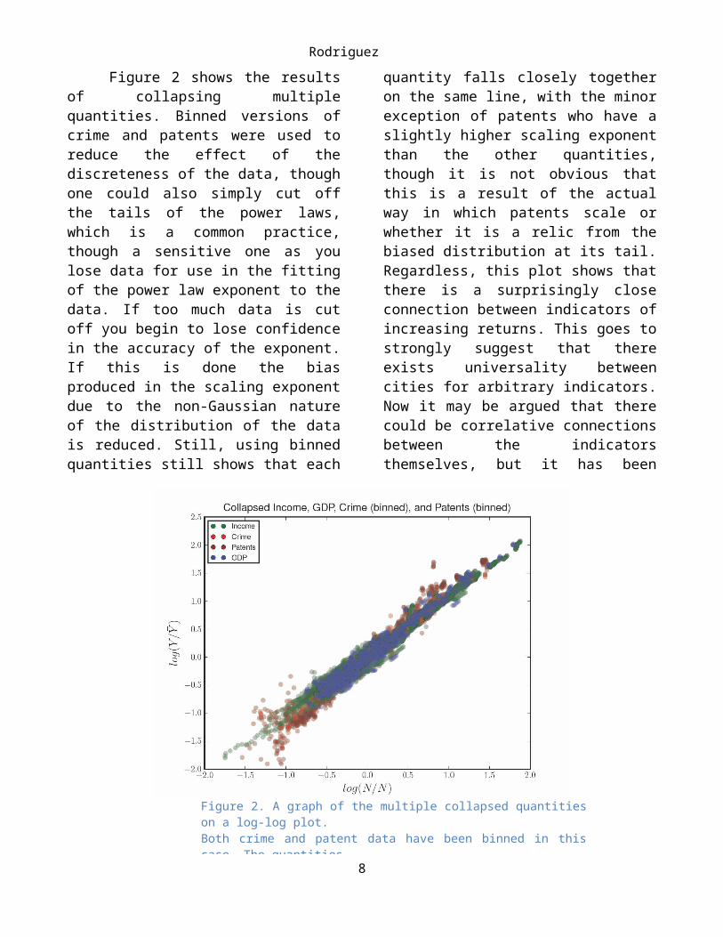
Figure 2 shows the results of collapsing multiple quantities. Binned versions of crime and patents were used to reduce the effect of the discreteness of the data, though one could also simply cut off the tails of the power laws, which is a common practice, though a sensitive one as you lose data for use in the fitting of the power law exponent to the data. If too much data is cut off you begin to lose confidence in the accuracy of the exponent. If this is done the bias produced in the scaling exponent due to the

non-Gaussian nature of the distribution of the data is reduced. Still, using binned quantities still shows that each quantity falls closely together on the same line, with the minor exception of patents who have a slightly higher scaling exponent than the other quantities, though it is not obvious that this is a result of the actual way in which patents scale or whether it is a relic from the biased distribution at its tail. Regardless, this plot shows that there is a surprisingly close connection between indicators of increasing returns. This goes to strongly suggest that there exists universality between cities for arbitrary indicators. Now it may be argued that there could be correlative connections between the indicators themselves, but it has been shown in recent research by Bettencourt and others (Bettencourt, et. al., 2010), that there exists only weak or no correlations between various indicators such as income and patents, or income and violent crime, to have some examples. To be clear, these are measuring the relative correlations between the quantities independent of population size. These results mean that

5

Figure 2. A graph of the multiple collapsed quantities on a log-log plot. Both crime and patent data have been binned in this case. The quantitiesfall closely on the same line, though patents has a slightly larger slopethan the other indicators.

Rodriguez

indicators can be considered to be essentially independent of each other to some degree.

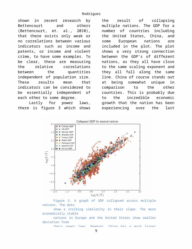
Lastly for power laws, there is figure 3 which shows the result of collapsing multiple nations. The GDP for a number of countries including the United States, China, and some European nations are included in the plot. The plot shows a very strong connection between the GDP’s of different nations, as they all have close to the same scaling exponent and they all fall along the same line. China of course stands out at being somewhat unique in comparison to the other countries. This is probably due to the incredible economic growth that the nation has been experiencing over the last decade. In contrast, the much more stable economies of the United States and Europe show much narrower distributions from the power law than in China. What is also interesting is the strange ‘hook’ that appears to separate itself from the rest of the distribution. This also has a physical explanation. China has a number of special

economic zones which are made to be attractive for foreign investors and allows more capitalistic practices. One of these, Shenzhen is arguably the most successful and prosperous city in China and it belongs to one of these special economic zones. In the 70’s Shenzhen was only a small fishing village, but now it is home to over 9 million people. The ‘hook’ in the data represents the city of Shenzhen. Its trail shows how over time it still follows the same power law scaling even though it is far removed from the rest of the distribution.

From these three cases we can argue in favor of the idea that there exist universally shared properties between cities regardless of time, quantity, or nation of origin with respect to scaling. What about the deviations from the power laws? As we have seen in the previous plots there are some interesting cases (China in particular) where the data deviates from the power law. Eying the plots qualitatively does not lend one to think that there could be a single

6

Figure 3. A graph of GDP collapsed across multiple nations. The datashow a striking similarity in their slope. The more economically stable nations in Europe and the United States show smaller deviation fromtheir power laws. However, China has a much larger spread in distri--bution. The ‘hook’ that is present in the Chinese GDP is representedby Shenzhen, the most prosperous city within the special economiczones of China.

Rodriguez

kind of distribution that would explain the behavior of all the residuals.

Residual DistributionsNow we will consider the deviations from the power laws. We define the residual as the difference between the power law and the data at any particular population size. The exact expression is:

ξ i=log (Y i )−log (Y o N iβ ) (5)

Where ξ is the residual, Y i is the observed quantity for a particular city, and the last term is the power law expressed for the population of that city. Essentially the residuals define the uniqueness of a city, as each city has its own deviation from the power law for each of its urban indicators, and this combination of residuals is specific to each city. These residuals have some interesting properties. They do not have a random distribution about

the power law, but rather exhibit a ‘long term memory’ as Luis Bettencourt describes it in his recent research (Bettencourt, et. al., 2010). Take for example San Jose, which is now known as Silicon Valley. It over performs relative to the power law in various quantities such as income and patents. If in 1969 San Jose is found to be over performing relative to the average, then it will continue to over perform for many decades. This effect is best shown in a plot borrowed from Luis’ paper (figure 4). The figure shows how the residuals for income remain relatively steady over many years. Cities that underperform continue to underperform, such as Brownsville, over many years. This is regardless of the many policies this city has no doubt enacted in an attempt to pull them out of relative poverty. This shows how ineffective current policies are at actually influencing long term growth or at changing the behavior of the city. Also indicated in the plot are gray bars which represent national periods

7

Figure 4. A plot of the residuals for income in the United states from 1969 through2006. The gray bars represent times of national recession. The plot shows the tendency of the residuals to remain steady over many decades, as well as theirrobustness in being unaffected by economic downturns. An special case is San Jose,whose residual spikes during the internet boom of the later 90’s and then falls toits previous levels following the respective bust in the early 2000’s.

Rodriguez

of recession. Even during these periods the residuals remain incredibly robust and appear not to be affected at all by these economic down turns. San Jose, however, is an interesting case as you can see how the internet boom and bust affect the city’s income. In this case the effects of the upward and downward market forces are clearly observed in the residuals, but even after the bust the residuals return to their pre-internet boom values! Bridgeport could also be considered another specific case as it is a banking town. So during times of recession when banks are affected by the economic downturn this urban system is more expressive of those changes.

Due to this nature of residuals a city taxonomy can be created (Bettencourt, et. al., 2010) which matches the performances of various urban centers independent of population size so you can gain a true relative performance indicator for an individual city with respect to others in the nation.

It is reasonable to ask whether similar universalities can be found as those discovered within power laws given this knowledge of the systematic behavior of residuals? To answer this question we look at the residuals in a collapsed form so that they can be presented together and so that we can draw out any similarities or differences in the distributions. This is done by taking the probability density function in terms of the particular quantity and eliminating parameters:

P (Y )= NsYln (10 )

e−|ln (Y /Y o N β )

ln (10) −μ|P

/ s (6)

P ( x )=N e−|x|P

(7)

In the first expression (6) there is the probability density of the quantity Y, where s is an estimator, μ is the mean of the residuals, and P is the exponent of the distribution. The other parameters are absorbed into x and eliminated through a change of variables. This leaves only the parameter P which we can then fit to the

data (7).Figure 5 shows an example fit for a

quantity collapsed over multiple years, in this case the GDP of the United States. This shows a very good correlation between the distributions of the data over several years, which suggests that there are indeed universal properties that hold from year. This similarity from year to year is expressed in the other quantities we looked at as well.

Figure 5b shows our collapse of the GDP for multiple nations. This uses the same data that we used in our plot of the collapsed GDP power laws, so this gives us a look at how the distributions relate. What is quite extraordinary is that China shares the same distribution as all the other nations, even though its cities had a much greater spread about the power law. This is an encouraging result as it helps support that even across nations this universality in distributions holds true.

We are currently working on collapsing the distributions for multiple quantities where we hope to discover the same sort of universality and complete this analysis.

3. DISCUSSION

What we have found from this research is that cities exhibit a large amount of universality across time, quantity, and origin, for both the power law relations and for deviations from the power law. This is quite an extraordinary result as it means that cities are robust systems that behave according to some very basic rules which are fundamental to the system and fairly independent of the environment. We can look at urban centers anywhere in the world and they will behave in approximately the same way as they are the same system. This raises some new and important questions like: What are the processes that give rise to these scaling laws and distributions? Why do these processes behave in the way that they do? And what are the rules that govern the development of these urban centers? Statistical analysis is not sufficient to answer all of these questions, but it has shed light on the empirical nature of cities.

8

Rodriguez

China represents a very important source of data to help us answer some of these deeper questions. The data for the United States only reliably goes back to 1969, which is not far enough for us to determine the origins and reasons why cities like San Jose became over performing in the first place, or why places like Brownsville struggle in relative poverty. Due to China’s fairly recent and extraordinary economic growth, new urban centers are being born with a high frequency, and data is available for us to look into the origins of cities like Shenzhen in a quantitative sense. This sort of analysis can help us better understand what underlying rules might govern the development of each city and how similar cities differentiate over time.

The Chinese data though can be difficult to work with as china does not have a definition for a metropolitan area in the sense that the U.S. and Europe do. Generally statistics are gathered based off of districts where data for the major city in that district is lumped together with the surrounding regions (ideally suburbs) under that cities administration. This is the closest to a metropolitan definition that China has at the moment. In addition to this the population of cities are determined from residency papers that are issued from the

government and which allow a person so live in certain area, however these tend to lead to underestimates of the actual population as there are many individuals that reside in these urban areas but do not have residency in them. For a large city such as Beijing, the official population and the actual population may differ by several million.

We plan on collapsing the distributions for multiple quantities soon; however we found some unsuspected distributions in the data for the United States related to income. We found that there is an asymmetry in the distribution of the residuals where there is an underrepresentation of very poor cities, while there is an overrepresentation of moderately underperforming cities. As we do not have income data for other nations we cannot determine yet if this is unique to the United States or if this is something general to other cities as well.

We have also found that a statistical approach using fitting and relying on the best R-squared value of the fit is insufficient to determine the kind of distribution the data follow, as our fitness landscapes are very shallow. So the difference in R-squared between a P value of 1 (exponential distribution) and a P value of 2 (normal

9

Figure 5. (a) A plot of the collapsed distributions of the GDP for the United States from 2001-2006. The distributions for each year are identical and fit very well to a curve that has an exponent around 1.6, which is in between the exponential and normal distributions. (b) A plot of the col-lapsed distributions of the GDP for multiple nations and years. The GDP from various nations fol-lows the same distribution which is again in between an exponential and normal. This plot uses the same data from figure 3 in the collapsing of the power laws.

Rodriguez

distribution) is not very large. We aim to solve this by creating a stochastic model that will help determine the origin of the distribution.

4. REFERENCES

Aaron Clauset , C. R. Shalizi, M. E. J. Newman, 2009, SIAM Review 51, 661-703, 2009

W. Morris, Architecture, Industry and Wealth: Collected Papers (Longmans, Green, and Co., London, 1902).

Michael Batty, Science vol 319, February 2008

L.M.A Bettencourt, et al., PNAS vol. 104 no. 17, April 24, 2007

L.M.A Bettencourt, et. al., in review PNAS, 2010

Horacio Samaniego, Melanie E. Moses, Journal of Transport and Land Use 1:1 (Summer 2008) pp. 21–39

10