statistical learning and optimization …statistical learning and optimization methods for ......

STATISTICAL LEARNING AND OPTIMIZATION METHODS FOR

IMPROVING THE EFFICIENCY IN LANDSCAPE IMAGE CLUSTERING

AND CLASSIFICATION PROBLEMS

SELIME GUROL

SEPTEMBER 2005

STATISTICAL LEARNING AND OPTIMIZATION METHODS FOR

IMPROVING THE EFFICIENCY IN LANDSCAPE IMAGE CLUSTERING

AND CLASSIFICATION PROBLEMS

A THESIS SUBMITTED TO

THE GRADUATE SCHOOL OF APPLIED MATHEMATICS

OF

THE MIDDLE EAST TECHNICAL UNIVERSITY

BY

SELIME GUROL

INPARTIALFULFILLMENTOFTHEREQUIREMENTSFORTHEDEGREEOF

MASTER OF SCIENCE

IN

THE DEPARTMENT OF SCIENTIFIC COMPUTING

SEPTEMBER 2005

Approval of the Graduate School of Applied Mathematics

Prof.Dr. Ersan AKYILDIZ

Director

I certify that this thesis satisfies all the requirements as a thesis for the degree of

Master of Science.

Prof. Dr. Bulent KARASOZEN

Head of Department

This is to certify that we have read this thesis and that in our opinion it is fully

adequate, in scope and quality, as a thesis for the degree of Master of Science.

Assist. Prof. Dr. Hakan Oktem

Supervisor

Examining Committee Members

Prof. Dr. Bulent Karasozen

Assoc. Prof. Dr. Tanıl Ergenc

Assist. Prof. Dr. A. Ozgur Kisisel

Assist. Prof. Dr. Hakan Oktem

Dr. Tamer Ozalp

I hereby declare that all information in this document has been obtained

and presented in accordance with academic rules and ethical conduct. I

also declare that, as required by these rules and conduct, I have fully

cited and referenced all material and results that are not original to this

work.

Name, Last name: Selime Gurol

Signature:

iii

abstract

STATISTICAL LEARNING AND OPTIMIZATION

METHODS FOR IMPROVING THE EFFICIENCY IN

LANDSCAPE IMAGE CLUSTERING AND

CLASSIFICATION PROBLEMS

Selime Gurol

M.Sc., Department of Scientific Computing

Supervisor: Assist. Prof. Dr. Hakan Oktem

Co-Supervisor: Prof. Dr. Bulent Karasozen

September 2005, 110 pages

Remote sensing techniques are vital for early detection of several problems such

as natural disasters, ecological problems and collecting information necessary for

finding optimum solutions to those problems. Remotely sensed information has

also important uses in predicting the future risks, urban planning, communication.

Recent developments in remote sensing instrumentation offered a challenge to the

mathematical and statistical methods to process the acquired information.

Classification of satellite images in the context of land cover classification is the

main concern of this study. Land cover classification can be performed by statistical

learning methods like additive models, decision trees, neural networks, k-means

methods which are already popular in unsupervised classification and clustering of

image scene inverse problems.

Due to the degradation and corruption of satellite images, the classification per-

formance is limited both by the accuracy of clustering and by the extent of the classi-

fication. In this study, we are concerned with understanding the performance of the

available unsupervised methods with k-means, supervised methods with Gaussian

maximum likelihood which are very popular methods in land cover classification.

A broader approach to the classification problem based on finding the optimal dis-

iv

criminants from a larger range of functions is considered also in this work. A novel

method based on threshold decomposition and Boolean discriminant functions is de-

veloped as an implementable application of this approach. All methods are applied

to BILSAT and Landsat satellite images using MATLAB software.

Keywords: Remote Sensing, Land Cover Classification, Classification Techniques,

Discriminant Function, Optimization, Statistical Learning, BILSAT

v

oz

GORUNTU KUMELENDIRME VE SINIFLANDIRMA

ALGORITMALARININ PERFORMANSINI ARTTIRMAK

ICIN ISTATISTIKSEL OGRENME VE OPTIMIZASYON

METODLARININ KULLANIMI

Selime Gurol

Yuksek Lisans, Bilimsel Hesaplama Bolumu

Tez Yoneticisi: Assist. Prof. Dr. Hakan Oktem

Ortak Tez Yoneticisi: Prof. Dr. Bulent Karasozen

Eylul 2005, 110 sayfa

Uzaktan algılama teknikleri; dogal afetler, ekolojik problemler gibi cesitli prob-

lemlerin erken farkedilmesinde ve bu problemlere optimum sonucların bulunması

icin gerekli bilginin elde edilmesinde hayati onem tasımaktadır. Uzaktan algılanan

bilginin aynı zamanda risk tahmini, kent planlaması ve haberlesme gibi alanlarda da

onemli bir kullanımı vardır. Uzaktan algılama enstrumantasyonundaki son gelismeler

elde edilen bilgileri anlamlı hale getirecek olan matematiksel ve istatistiksel metod-

ların onemini artırmıstır.

Bu calısma genel olarak uydu goruntulerinin arazi ortusu sınıflandırmasını icer-

mektedir. Arazi ortusu sınıflandırılması, halen goruntulerin kumelenmesi ve sınıflan-

dırılması icin kullanılan toplamsal metodlar, karar verici agaclar, yapay sinir agları,

k-ortalama metodları gibi populer istatistiksel metodlarla gerceklestirilebilir.

Goruntunun bozulması ve gurultu gibi etkenler nedeniyle goruntu kumelendirme

ve sınıflandırma algoritmaları hem performans acısından hem de yapılabilir sınıflan-

dırmanın detayı acısından sınırlıdır. Bu calısmada arazi ortusu sınıflandırmasında

kullanılan populer metodların performansını anlamak icin egitimsiz sınıflandırmada

k-ortalama yontemi ve egitimli sınıflandırmada da Gauss maksimum olabilirlik yonte-

vi

mi kullanılmıstır. Sınıflandırma probleminin cozumu icin bu metodlara alternatif

olarak, daha genis bir fonksiyon kumesinden optimum ayırt edici fonksiyonu bul-

maya dayalı bir yaklasım dusunulmustur. Bu yaklasımın uygulanabilmesi icin esik

ayrıstırma ve Boolean ayırt edici fonksiyonlarına dayanan ozgun bir yontem gelistiril-

mistir. Butun yontemler BILSAT ve Landsat uydu goruntuleri kullanılarak MAT-

LAB yazılımında test edilmistir.

Anahtar Kelimeler: Uzaktan Algılama, Arazi Ortusu Sınıflandırması, Sınıflandırma

Teknikleri, Ayırt Edici Fonksiyon, Optimizasyon, Istatistiksel Ogrenme, BILSAT

vii

To my family

viii

ACKNOWLEDGMENT

I would like to express my gratitude to my advisor, Assist Prof. Dr. Hakan

Oktem, for his friendship, exemplary effort and support during this study.

I would like to thank Prof. Dr. Bulent Karasozen for his valuable contribution

to this study. I also thank Prof. Dr. Gerhard Wilhelm Weber for his friendship and

support.

My sincere thanks go to Dr. Tamer Ozalp whose guidance, support and advice

began before this study encouraged me to concern over remote sensing area. Spe-

cial thanks to European Space Agency and International Space University for their

contribution during this study. This contribution has broadened my perspective on

remote sensing.

Sincere thanks to Micheline Tabache, member of ESA International Relations

Department, for her support and valuable contribution during this study.

I am grateful to my friend Didem for her sharing this hard period with me,

encouragement, understanding, patience and guidance throughout this study. I am

thankful to my friend Aslı and my homemate Bilge for not feeling myself alone and

motivating me.

I would like thank to my aunt Zeynep Akcay for her encouragement, advice and

support during my study.

It is very important for the continuation of the study to be in a peaceful place

which is supported during all my study from my institute. So, thanks each of IAM

(Institute of Applied Mathematics) members to feel myself in comfort.

This work was supported by The Scientific and Technical Research Council of

Turkey MSc. Scholarship Program (TUBITAK Yurt Ici Yuksek Lisans Burs Pro-

gramı).

Special thanks to BILTEN (Information Technologies and Electronics Research

Institute) and IKONOS Space Imaging for supplying the data which is very critical

for this study.

None of my study would have been possible without the support of my family.

Thanks each of them for their continuous support and endless patience.

ix

table of contents

plagiarism . . . . . . . . . . . . . . . . . . . . . . . . . . . . . . . . . . . . . . . . . . . . . . . . . . . . iii

abstract . . . . . . . . . . . . . . . . . . . . . . . . . . . . . . . . . . . . . . . . . . . . . . . . . . . . . iv

oz . . . . . . . . . . . . . . . . . . . . . . . . . . . . . . . . . . . . . . . . . . . . . . . . . . . . . . . . . . . . . vi

acknowledgements . . . . . . . . . . . . . . . . . . . . . . . . . . . . . . . . . . . . . . . . . ix

table of contents . . . . . . . . . . . . . . . . . . . . . . . . . . . . . . . . . . . . . . . . . . x

list of tables . . . . . . . . . . . . . . . . . . . . . . . . . . . . . . . . . . . . . . . . . . . . . . . . xiii

list of figures . . . . . . . . . . . . . . . . . . . . . . . . . . . . . . . . . . . . . . . . . . . . . . . xv

list of abbreviations and acronyms . . . . . . . . . . . . . . . . . . . . . .xviii

CHAPTER

1 INTRODUCTION . . . . . . . . . . . . . . . . . . . . . . . . . . . . . . . . . . . . . . . . . 1

1.1 Purpose and Scope . . . . . . . . . . . . . . . . . . . . . . . . . . . . 2

1.2 Study Area . . . . . . . . . . . . . . . . . . . . . . . . . . . . . . . . 3

1.3 Background . . . . . . . . . . . . . . . . . . . . . . . . . . . . . . . . 5

1.4 Literature Survey . . . . . . . . . . . . . . . . . . . . . . . . . . . . . 12

1.5 Field Survey . . . . . . . . . . . . . . . . . . . . . . . . . . . . . . . . 16

1.6 Data Characteristics Used in the Study . . . . . . . . . . . . . . . . . 22

1.6.1 BILSAT-1 Data . . . . . . . . . . . . . . . . . . . . . . . . . . 22

1.6.2 Landsat-7 Data . . . . . . . . . . . . . . . . . . . . . . . . . . 23

1.6.3 IKONOS Data . . . . . . . . . . . . . . . . . . . . . . . . . . 24

x

2 DATA ANALYSIS . . . . . . . . . . . . . . . . . . . . . . . . . . . . . . . . . . . . . . . . . 25

2.1 Image Rectification and Restoration . . . . . . . . . . . . . . . . . . . 27

2.1.1 Geometric Correction . . . . . . . . . . . . . . . . . . . . . . . 27

2.1.2 Radiometric Correction . . . . . . . . . . . . . . . . . . . . . . 28

2.1.3 Noise Removal . . . . . . . . . . . . . . . . . . . . . . . . . . 29

2.2 Image Enhancement . . . . . . . . . . . . . . . . . . . . . . . . . . . 30

3 IMAGE CLASSIFICATION . . . . . . . . . . . . . . . . . . . . . . . . . . . . . . 31

3.1 Problem Statement . . . . . . . . . . . . . . . . . . . . . . . . . . . . 32

3.2 Classification Techniques . . . . . . . . . . . . . . . . . . . . . . . . . 35

3.3 Unsupervised Classification . . . . . . . . . . . . . . . . . . . . . . . 36

3.3.1 K-Means Classification Method . . . . . . . . . . . . . . . . . 37

3.4 Supervised Classification . . . . . . . . . . . . . . . . . . . . . . . . . 39

3.4.1 Gaussian Maximum Likelihood Classification Method . . . . . 40

3.5 A Generalization of Distribution Free

Classification . . . . . . . . . . . . . . . . . . . . . . . . . . . . . . . 42

3.6 Threshold Decomposition and Boolean Discriminant Functions . . . . 43

3.7 Factors that Affect the Classification

Performance . . . . . . . . . . . . . . . . . . . . . . . . . . . . . . . . 55

3.8 Classification Accuracy Assessment . . . . . . . . . . . . . . . . . . . 56

4 CLASSIFICATION RESULTS . . . . . . . . . . . . . . . . . . . . . . . . . . . 59

4.1 K-Means Classification . . . . . . . . . . . . . . . . . . . . . . . . . . 61

4.2 Gaussian Maximum Likelihood Classification . . . . . . . . . . . . . . 67

4.3 Boolean Discriminant Function Classifier . . . . . . . . . . . . . . . . 75

4.4 Comparision of Methods . . . . . . . . . . . . . . . . . . . . . . . . . 81

5 CONCLUSION AND DISCUSSIONS . . . . . . . . . . . . . . . . . . . 89

references . . . . . . . . . . . . . . . . . . . . . . . . . . . . . . . . . . . . . . . . . . . . . . . . . . . 91

xi

APPENDICES

A. FILE booleanthresh.m . . . . . . . . . . . . . . . . . . . . . . . . . . . . . . . . . . 100

B. BILSAT IMAGE OF METU SETTLEMENT . . . . . . . 109

C. LANDSAT IMAGE OF METU SETTLEMENT . . . . 110

xii

list of tables

1.1 Spectral Bands Characteristics [57]. . . . . . . . . . . . . . . . . . . . 6

1.2 BILSAT imagery characteristics. . . . . . . . . . . . . . . . . . . . . . 22

1.3 Landsat 7 ETM+ imagery characteristics. . . . . . . . . . . . . . . . 23

1.4 IKONOS imagery characteristics. . . . . . . . . . . . . . . . . . . . . 24

4.1 CPU time for each classifier using Landsat-7 RGB image. . . . . . . . 82

4.2 CPU time for each classifier using BILSAT RGB image. . . . . . . . . 82

4.3 Error matrix of classification results of Landsat RGB imagery with

K-means classifier (six class).* . . . . . . . . . . . . . . . . . . . . . 83


K-means classifier (five class).* . . . . . . . . . . . . . . . . . . . . . 83

4.5 Error matrix of classification results of BILSAT RGB imagery with

K-means classifier (six class).* . . . . . . . . . . . . . . . . . . . . . . 84


K-means classifier (five class).* . . . . . . . . . . . . . . . . . . . . . 84


maximum likelihood classifier (six class).* . . . . . . . . . . . . . . . 85


maximum likelihood classifier (five class).* . . . . . . . . . . . . . . . 85


maximum likelihood classifier (six class).* . . . . . . . . . . . . . . . 86


maximum likelihood classifier (five class).* . . . . . . . . . . . . . . . 86


Boolean discriminant function (six class).* . . . . . . . . . . . . . . . 87


Boolean Discriminant Function (five class).* . . . . . . . . . . . . . . 87


Boolean discriminant function (six class).* . . . . . . . . . . . . . . . 88

xiii


Boolean discriminant function (five class).* . . . . . . . . . . . . . . . 88

xiv

list of figures

1.1 Location map of study area (METU) [56]. . . . . . . . . . . . . . . . 3

1.2 Different views from satellite RGB images of the study area acquired

from reference [69]. . . . . . . . . . . . . . . . . . . . . . . . . . . . . 4

1.3 Electromagnetic Spectrum [70]. . . . . . . . . . . . . . . . . . . . . . 7

1.4 A Typical Satellite Based Remote Sensing System. . . . . . . . . . . 8

1.5 Atmospheric electromagnetic transmittance [67]. . . . . . . . . . . . . 9

1.6 Electromagnetic waves interaction with the target. (A:Absorption,

T: Transmission, R: Reflection, I: Incidence) [68]. . . . . . . . . . . . 10

1.7 Relation between ab and DN output [53]. . . . . . . . . . . . . . . . . 10

1.8 Built-up Land. . . . . . . . . . . . . . . . . . . . . . . . . . . . . . . 16

1.9 Builtup view from airphoto. . . . . . . . . . . . . . . . . . . . . . . . 17

1.10 Agricultural Land. . . . . . . . . . . . . . . . . . . . . . . . . . . . . 18

1.11 Agricultural Land view from airphoto. . . . . . . . . . . . . . . . . . 18

1.12 Forest Land. . . . . . . . . . . . . . . . . . . . . . . . . . . . . . . . . 19

1.13 Forest Land view from airphoto. . . . . . . . . . . . . . . . . . . . . . 19

1.14 Lake Eymir. . . . . . . . . . . . . . . . . . . . . . . . . . . . . . . . . 20

1.15 Lake Eymir view from airphoto. . . . . . . . . . . . . . . . . . . . . . 20

1.16 Mixed Barren Land. . . . . . . . . . . . . . . . . . . . . . . . . . . . 21

1.17 Barren Land view from airphoto. . . . . . . . . . . . . . . . . . . . . 21

2.1 Data Analysis Flow. . . . . . . . . . . . . . . . . . . . . . . . . . . . 26

2.2 Example to the geometric correction by nearest neighbor method. . . 27

2.3 Image enhancement of image includes METU settlement from BIL-

SAT red channel. . . . . . . . . . . . . . . . . . . . . . . . . . . . . 30

3.1 State Space Representation. . . . . . . . . . . . . . . . . . . . . . . . 33

3.2 Classification Techniques. . . . . . . . . . . . . . . . . . . . . . . . . 35

4.1 BILSAT training data characteristics of RGB and NIR band . . . . . 60

xv

4.2 Landsat-7 training data characteristics of RGB and NIR bands . . . . 60

4.3 Classification of Landsat-7 RGB imagery using k-means classifier. . . 62

4.4 Classification of BILSAT RGB imagery using k-means classifier. . . . 63

4.5 Classification of Landsat-7 RBnir imagery using k-means classifier . . 64

4.6 Classification of BILSAT RBnir imagery using k-means classifier . . 64

4.7 Classification of Landsat-7 RGB imagery using k-means classifier . . 65

4.8 Classification of BILSAT RGB imagery using k-means classifier . . . 65

4.9 Classification of Landsat-7 RBnir imagery using k-means classifier . . 66

4.10 Classification of BILSAT RBnir imagery using k-means classifier . . . 66

4.11 Histograms of each training class of BILSAT imagery . . . . . . . . . 67

4.12 Probability density functions of each training class of BILSAT im-

agery of each training class . . . . . . . . . . . . . . . . . . . . . . . . 68

4.13 Histograms of each training class of Landsat imagery . . . . . . . . . 68

4.14 Probability density functions of each training class of Landsat imagery 69

4.15 Classification of Landsat RGB imagery using Gaussian maximum

likelihood classifier . . . . . . . . . . . . . . . . . . . . . . . . . . . . 70

4.16 Classification of BILSAT RGB imagery using Gaussian maximum


4.17 Classification of Landsat RBnir imagery using Gaussian maximum


4.18 Classification of BILSAT RBnir imagery using Gaussian maximum


4.19 Classification of Landsat RGB imagery using Gaussian maximum


4.20 Classification of Landsat RBnir imagery using Gaussian maximum


4.21 Classification of BILSAT RGB imagery using Gaussian maximum


4.22 Classification of BILSAT RBnir imagery using Gaussian maximum


4.23 Classification of Landsat RGB imagery using Boolean discriminant

function classifier . . . . . . . . . . . . . . . . . . . . . . . . . . . . . 76

xvi

4.24 Classification of BILSAT RGB imagery using Boolean discriminant


4.25 Classification of Landsat RBnir imagery using Boolean discriminant


4.26 Classification of BILSAT RBnir imagery using Boolean discriminant


4.27 Classification of Landsat RGB imagery using Boolean discriminant


4.28 Classification of Landsat RBnir imagery using Boolean discriminant


4.29 Classification of BILSAT RGB imagery using Boolean discriminant


4.30 Classification of BILSAT RBnir imagery using Boolean discriminant


4.31 Classification with Boolean discriminant function using 100 threshold

levels . . . . . . . . . . . . . . . . . . . . . . . . . . . . . . . . . . . . 81

xvii

LIST OF ABBREVIATIONS AND ACRONYMS

AIAA American Institute of Aeronautics and Astronautics

ARTMAP Adaptive Resonance Theory

ANN Artificial Neural Network

BILTEN Information Technologies and Electronics Research Institute

BILSAT-1 BILTEN Satellite-1

DN Digital Number

DTC-LSMA Decision Tree Classification based on Linear Spectral Mixture Analysis

ECHO Extraction and Classification of Homogeneous Objects

EOSAT Earth Observation Satellite

ERDAS Earth Resources Data Analysis System (Commercial software)

ERTS-1 Earth Resources Technology Satellite-1

ESA European Space Agency

ETM+ Enhanced Thematic Mapper Plus

GIS Geographic Information System

IFOV Instantaneous Field Of View

ISU International Space University

KHTT Know-How Transfer and Training

Landsat-1 Land Satellite-1

MATLAB Matrix Laboratory(A commercial software by MATHworks Inc.)

METU Middle East Technical University

MLC Maximum Likelihood Classifier

NASA National Aeronautics and Space Administration

PSF Point Spread Function

RGB Red Green Blue

SNR Signal-to-Noise Ratio

SOM Self Organized feature Map

SPOT-1 Satellite Pour l’Observation de la Terre-1

SSTL Surrey Satellite Technology Limited

TUBITAK The Scientific and Technical Research Council of Turkey

xviii

chapter 1

INTRODUCTION

The impacts of real world problems such as natural disasters, global warming,

limited water resources are increasing day by day together with the complexity of

handling these impacts on humanity and nature. As a result, effective and sustain-

able future management of earth requires continuous monitoring of our planet.

A lot of scientific and socio-economic research is being held to understand those

problems. Remote sensing is the quickest method to detect the above mentioned

problems as early as possible or predict the future risks as accurate as possible with

an optimum cost. In [21, 34], remote sensing is defined as the science, art and

technology of obtaining reliable information about an object, area, or phenomenon

through the analysis of data acquired by a device that is not in contact with the

object, area, or phenomenon. This remotely acquired information has also the

potential to be used in finding out global solutions to those problems.

The first use of the term remote sensing is in the 1960’s. NASA established a

research program in remote sensing in the 1960’s. In the 1970’s remote sensing is

also started to be used in civil applications after launching of Landsat-1. Remote

sensing started to play a very important role in technology, and other countries

launched their own earth observation satellites in following years. In Turkey, remote

sensing studies were started in the 1980’s. Turkey had its first earth observation

satellite BILSAT-1 in September 2003.

Remote sensing has lots of application areas including meteorology, climatology,

geology, archeology, military, land cover/land use, planetary studies, etc.. In this

study, land cover classification is the main concern.

During the development of remote sensing, considerable research has been de-

voted to image classification for obtaining high quality of thematic-maps which are

the important outputs of remote sensing system.

1

In the system of remote sensing, there are many error sources which affect the

accuracy of the classified image according to the ground truth data. These errors

can occur in acquisition, data processing, data analysis, data conversion, and in

decision making phases. In this study, the errors originated from data classification

phase are concerned.

The classification of pixels of an image is performed by employing a difference

metric or a classifier function. Most of the conventional methods in literature are

based on a predetermined classifier like Euclidian distance from the class mean,

k-nearest neighbor algorithm, minimum distance classifier, Gaussian maximum like-

lihood, etc.. However, due to the several reasons including noise in the images,

non-unique distribution of the data into classes, existence of texture type of fea-

tures, dependence of the brightness values to the angle of the projection, etc., the

performance of those conventional algorithms are around 65 % which is not sufficient

for many applications. A broader approach to this problem is finding the optimal

discriminants from a larger range of functions. An implementable application of this

approach can be using threshold decomposition and Boolean discriminant functions

to partition the feature space into subspaces each corresponding to a class.

1.1 Purpose and Scope

In this study remote sensing especially for land cover classification was investi-

gated by using satellite data. The study was mainly focused on the concept of clas-

sification methods. Basically, unsupervised and supervised learning techniques were

applied to better understanding land cover classification of the study area. These

are statistical and distribution free methods. Secondly the study was directed to

develop an algorithm for each method in MATLAB. After that the methods were

implemented and compared to get better performance of the used algorithms. Fi-

nally, the research was designed to show different perspectives for the investigated

problem.

2

1.2 Study Area

Middle East Technical University (METU) settlement was chosen to implement

the classification methods and to test the performance of each classifier. The reason

for studying this location is its covering various landscape features in a distance that

we can make a field study easily. METU campus is located on the Ankara-Eskisehir

highway about 20 kilometers from the centrum of Ankara (see Figure 1.1 and 1.2).

The campus area is 4500 hectares and the forest area is 3043 hectares, including

Lake Eymir [72]. Since the early 1960’s the area has been forested by voluntary

university employees and students. Originally the area is almost bare soil, which is

typical for Central Anatolia [56].

Figure 1.1: Location map of study area (METU) [56].

3

Figure 1.2: Different views from satellite RGB images of the study area acquiredfrom reference [69].

4

1.3 Background

The first application in aerial remote sensing was started by using the balloons

in the late 1700’s. Balloons, kites, and pigeons were used for obtaining the com-

prehensive view of the earth. During the first and second world war there were so

many improvements in the area of military and civil remote sensing. The modern

era of remote sensing began with the first dedicated civil remote sensing satellite,

NASA Earth Resources Technology Satellite (ERTS-1). It was conceived in 1965

and launched on July 23, 1972 with the name of Landsat-1. Then, the system

was commercialized by transferring the system to the Earth Observation Satellite

Cooperation. After that France joined this commercial remote sensing market by

launching SPOT-1 in 1986. Many operational civil remote sensing satellites have

been launched by several international and national organizations like ESA, Canada,

Japan, Russia, India and Turkey for twenty years [21, 53].

The critical point of remote sensing from its definition is acquiring information

by measuring at a distance, rather than in situ. This appears as an advantage of

receiving a repetitive and coherent view of earth in small periods of time with a

wide range of landscape.

The remotely collected data can be of many forms including variations in force

distributions, acoustic wave distributions, or electromagnetic energy distributions

[34]. Most of the application areas in remote sensing require data obtained from

electromagnetic waves. Sensors placed on a satellite or aircraft records electro-

magnetic waves (see Figure 1.3) from different spectral bands to meet the need of

different data users (see Table 1.1). Therefore, the system map, monitor earth re-

sources and provide useful information for scientific, commercial or public service

activities.

A typical remote sensing system consists of subsystems (see Figure 1.4). It

requires two complex processing units which are data acquisition and data analysis

to obtain information about phenomena under investigation. The steps followed in

Figure 1.4 are:

(1) Energy Source: Remote sensing sytem’s fundamental expose is the energy

source. The system takes an action with this source which exposes electromagnetic

5

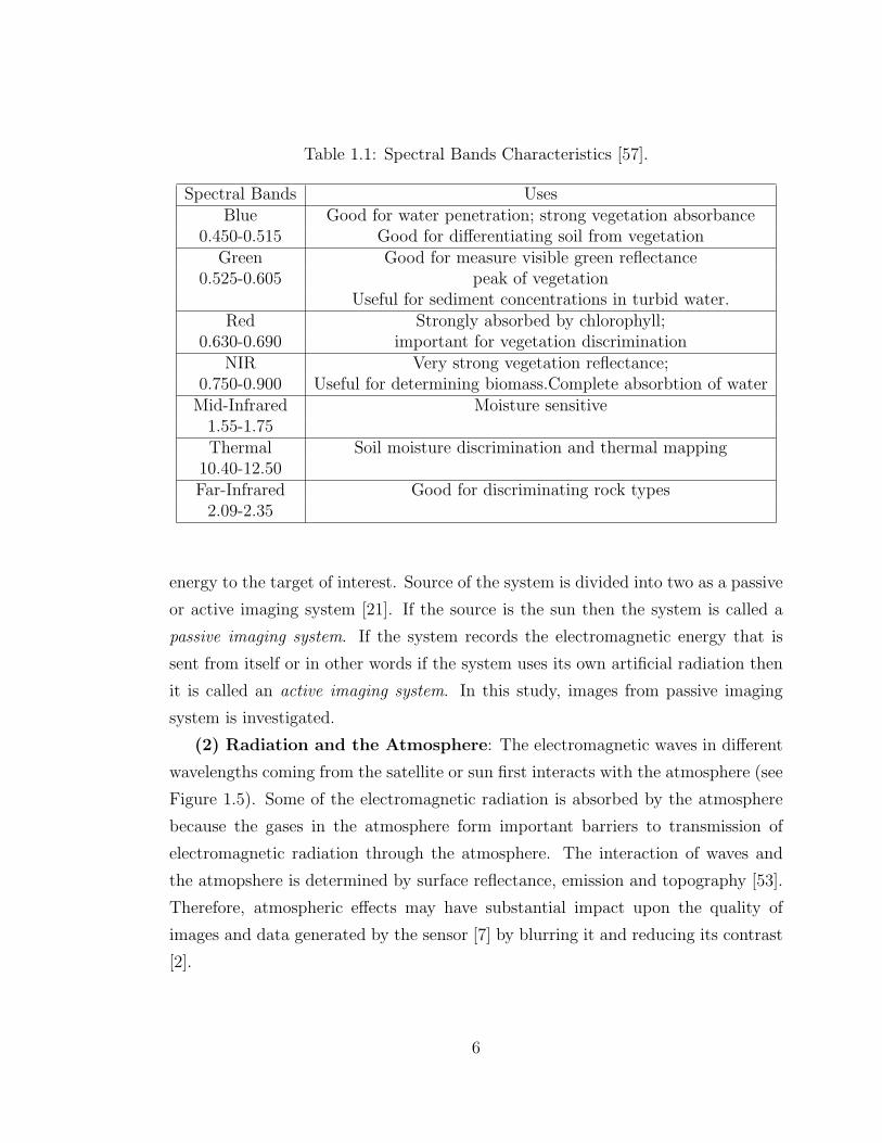
Table 1.1: Spectral Bands Characteristics [57].

Spectral Bands UsesBlue Good for water penetration; strong vegetation absorbance

0.450-0.515 Good for differentiating soil from vegetationGreen Good for measure visible green reflectance

0.525-0.605 peak of vegetationUseful for sediment concentrations in turbid water.

Red Strongly absorbed by chlorophyll;0.630-0.690 important for vegetation discrimination

NIR Very strong vegetation reflectance;0.750-0.900 Useful for determining biomass.Complete absorbtion of water

Mid-Infrared Moisture sensitive1.55-1.75Thermal Soil moisture discrimination and thermal mapping

10.40-12.50Far-Infrared Good for discriminating rock types

2.09-2.35

energy to the target of interest. Source of the system is divided into two as a passive

or active imaging system [21]. If the source is the sun then the system is called a

passive imaging system. If the system records the electromagnetic energy that is

sent from itself or in other words if the system uses its own artificial radiation then

it is called an active imaging system. In this study, images from passive imaging

system is investigated.

(2) Radiation and the Atmosphere: The electromagnetic waves in different

wavelengths coming from the satellite or sun first interacts with the atmosphere (see

Figure 1.5). Some of the electromagnetic radiation is absorbed by the atmosphere

because the gases in the atmosphere form important barriers to transmission of

electromagnetic radiation through the atmosphere. The interaction of waves and

the atmopshere is determined by surface reflectance, emission and topography [53].

Therefore, atmospheric effects may have substantial impact upon the quality of

images and data generated by the sensor [7] by blurring it and reducing its contrast

[2].

6

Figure 1.3: Electromagnetic Spectrum [70].

When the energy interacts with the Earth surface, some is scattered, some is

absorbed by the target and some is reflected (see Figure 1.6). Reflection, absorbtion

and transmission rates of the radiation depends on the nature of the surface, the

wavelength of energy and the incident angle. While the energy go back through the

direction of satellite, it is again absorbed by the atmosphere. The sensor records

this remaining energy for an input to obtain the raw data of the interested area

[68, 7].

(3) Sensor: There should be an electromagnetic sensor to collect and record

the total electromagnetic radiation in various wavelength regions known as spec-

tral bands which is reflected from the earth surface. The sensor records energy in

different bands because measurements over several spectral bands make up a ”spec-

tral response pattern”, or ”signature” which is unique to an object at a specific

temperature [21].

Sensor characteristics are determined by spatial resolution (size of the picture

element), radiometric resolution (smallest detected and quantified increment of ex-

posure), spectral resolution (wavelength bandwidths and number of bands) and

temporal resolution (frequency of covering the same area by the same instrument)

which directly affect the data quality and assist in choosing the right data for various

applications [30].

Some types of sensors according to the aim of the investigation are atmospheric

7

Figure 1.4: A Typical Satellite Based Remote Sensing System.

chemistry instruments, cloud profile and rain radars, earth radiation budget ra-

diometers, high resolution optical imagers, imaging microwave radars, Lidars, Ocean

colour instruments, radar altimeters, scatterometers [8].

(4) Transmission, Reception, and Processing: In electro-optical remote

sensing, the recording elements produce an electrical signal, and this signal is recorded

in a digital form [21]. This digitized image can then be processed by computer [24].

The electronic signal formulation can be given as:

eb(x, y) =

αmax∫αmin

βmax∫βmin

sb(α, β)PSFnet(x− α, y − β)dαdβ,

where eb is the electronic signal in band b, sb is the signal measured by the sensor,

PSFnet is the Point Spread Function (PSF) which is a weightening function for a

spatial convolution, (x, y) represent the coordinates and the limits of the integral

8

Figure 1.5: Atmospheric electromagnetic transmittance [67].

(α, β) define the spatial extent of the PSF about the coordinate (x, y) [53]. Then,

this electronic signal is amplified electronically and filtered by the electronics PSF.

The amplification stage is designed to provide sufficient signal level to A/D for

quantization, without incurring saturation.

The data is sampled as

ab(i, j) = ab(i4x, j4y),

where 4x and 4y are the sampling periods.

For quantization the amplified signal, ab, is sampled and each sample is quantized

into digital numbers (DN) using a finite number of bits [24]. The final DN at pixel

p and band b is,

DNpb = int[ab],

where int[ ] operator converts the output of the signal amplifier to the nearest

9

Figure 1.6: Electromagnetic waves interaction with the target. (A:Absorption, T:Transmission, R: Reflection, I: Incidence) [68].

integer value (see Figure 1.7) [53]. In Figure 1.7, Q (the number of bits/pixel)

defines the radiometric resolution of the system [53]. The number of discrete DNs

are determined by Q.

Figure 1.7: Relation between ab and DN output [53].

As a summary, the instrument receives all the radiation from a certain area on the

ground (IFOV) and generates a response. The signal of interest is degraded by the

sensor during this transformation. Therefore, it is important a deep understanding

of this degradation for designing the algorithms of image processing [53].

The signal attributed to any given pixel arises as a result of contributions not

only from the field of view corresponding to that pixel but also includes contributions

that properly belong to neighboring pixels. The pixel intensities are not independent

but there is an autocorrelation among them [12]. While designing the classification

algorithm, it is important to take into consideration of the neighbouring pixels.

10

(5) Interpretation and Analysis: Until now data acquisition process is ex-

plained. After this process the raw data is obtained and ready for data analysis.

The remotely sensed data analysis consists of two elements, digital processing and

visual interpretation.Visual interpretation and digital image processing should allow

the analyst to perform scientific visualization, defined as “visually exploring data

and information in such a way as to gain understanding and insight into the data”

[26].

For processing the digital data some preprocessing operations including geomet-

ric correction, radiometric correction, noise removal, masking should be done to cor-

rect the distorted or degraded image data. These procedures are also important in

the comparison of the two images obtained from different sensors. After preprocess-

ing is complete, the analyst may use feature extraction to reduce the dimensionality

of the data or change the dimensions according to the desired solutions. Therefore,

the physical feature on the Earth’s surface is converted to a useful information in

the data, known as feature with a transformation function.

The analyst chooses one of the classification techniques according to the purpose

of the study and data set to assign each pixel to a specific class using their spectral

characteristics. The feature space is used as an input to the classification procedure.

So, individual pixels are grouped according to their similarities determined by the

analyst. These groups could be specific regions which have common geologic prop-

erties which make it possible to derive information about land use, vegetation type

etc. After classification is completed, accuracy assessment should be done to have

the knowledge of what is the performance of the analyst’s results.

The output of the analysis could be maps, data and a report. These three

elements of results give the user information about the data source, the method of

analysis, the outcome and its reliability [7].

(6) Application: The final data of the remote sensing is integrated with the

other outputs to better understand the target information, reveal some new infor-

mation and help to solve complex problems. The integration of classified remotely

sensed data types requires accurate registration of various data layers, spatial data

infrastructure and standards, classification schemes, accuracy of each data layer, use

of positioning systems, data compability, and selection of appropriate spatial mod-

11

elling techniques [21]. This system, a computerized system, designed to enter, store,

manipulate,analyze and display the spatial data is called Geographic Information

System (GIS).

Until this part, overview of remote sensing field is pointed out. Like other fields,

lots of data are generated in remote sensing. In this study, the aim is to extract

important patterns and trends, and learn necessary information from the data [19].

The learning problems can be grouped as supervised and unsupervised. In unsu-

pervised learning or clustering, tha aim is to group a given collection of unlabeled

patterns into meaningful clusters [25]. In supervised learning, the goal is to pre-

dict the outputs according to the priori knowledge about the data. In this study,

unsupervised and supervised learning concepts are handled for the satellite image

classification purpose.

1.4 Literature Survey

The expected global changes to the earth system make the information about our

environment vital for the effective and sustainable future management [8]. Since the

1970’s, scientists have been developing the field of remote sensing for this purpose.

One of the most important applications in remote sensing is land cover classification

which is pointed out in this study.

Classification is the process of the assignment of a phenomena to a predefined

category. As a result of the development in digital computing, classification tech-

niques were developed by many disciplines, including statistics, communication the-

ory, biology, psychology, linguistics, and computer science besides remote sensing

[64]. Classification techniques were improved generally through the main techniques

including unsupervised and supervised classification techniques. There are different

criteria for optimal classification that include minimizing the probability of error

[15] and minimizing the average cost of a decision [64].

In the context of remote sensing, classification takes into account the reflectance

spectrum of land covers additionally in some cases spatial context information such

as slope and texture. Since remote sensing has become very popular for 20 years,

there are lots of studies related with this research area. The majority of articles stud-

12

ied in this work are concerned with land cover mapping by using the multispectral

data obtained from the passive remote sensing system.

In general, we can classify the studies related with classification into two ac-

cording to their aim. One group is focused on the improvement of the classification

process, others on the use of well-known classification methods through the types

of remote sensing applications [29, 31, 37, 61, 60]. The classificaton process can be

generalized with the following diagram [60].

Schematic of classification process.

During the 15 years period, the improvements in classification take place in three

directions:

1. The development of classification algorithm including training strategy and ap-

proaches to seperate feature space into classes based on statistical or distribution-

free methods [60].

2. The development of novel-systems level approaches that augment the under-

lying classifier algorithms, e.g. fuzzy classifiers [60].

3. The exploitation of multiple types of data or ancillary information, both nu-

merical or categorical, in a classification process [60].

13

Beginning with the simplest approach to classification, unsupervised classification

has the advantages over others when there is no priori information about area under

consideration. Kartikeyan et al. [28] discussed unsupervised classification problems

and propose a new technique for the segmentation of multispectral remote sensing

imagery. Also Jain et al. [25] gave a review about data clustering.

When sufficient information about the imagery to be classified is obtained, one

of the most common and widespread supervised method is Gaussian maximum like-

lihood classification method [13]. Jackson and Langrebe [23] contributed to the de-

velopment of the supervised maximum likelihood method which is based on the

statistical assumptions.

Distribution free methods such as neural networks [59], and decision trees [45]

are developed as an alternative to the methods that require statistical frequency

distribution. Yoshida and Omatu [62] developed a decision tree classifier based on

linear spectral mixture and state that it has good performance to address the land-

cover heterogeneity.

The reason for the decision tree methods to become popular in classification can

be ordered as [18, 45]: its ability to handle data measured on different scales, lack

of any assumptions concerning the distributions of the data in each of the classes,

flexibility and ability to handle non-linear relationships between features and classes.

Neural networks have been developed for ten years and majority find that this

method produce similar or superior performance with respect to the maximum like-

lihood classifier (MLC) [6, 20, 36, 46]. The most popular neural network technique

is back propagating multi layer perceptron neural network [20, 45, 46]. The others

can be ordered as binary diamond neural networks [51], delta rule and generalized

delta rule [5]. Also, Porter et al. [49] proposed a new network architecture. The

main disadvantage of this method is the fact that it is not computationally efficient

as the others.

There are so many articles comparing these methods. Benediktsson et al., Paola

and Schowengerdt [5, 46] compared neural networks and statistical methods. Pal

and Paul [45] made a comparision between decision tree, MLC and neural networks.

Another approach is combining different classifiers in one classifier, named as

hybrid classifier in the literature, e.g. a hybrid classifer approach using Decision

14

Tree and ARTMAP (Adaptive Resonance Theory) neural network [35], MLC and

decision tree [38]. Also, Extraction and Classification of Homogeneous Objects

(ECHO) classifier which is part of the MultiSpec software package that has been

developed at Purdue University and funded by NASA can be given as an example

to hybrid classifiers. ECHO is a multistage spectral-spatial classifier that combines

spectral and spatial/textural features; hence it is hybrid in character [37, 62]. Kelly

et al. [29] compared hybrid systems with the usual classification methods. McCauley

and Engel [41] compared ECHO and MLC.

Recently, there are new developments on the optimization of the classifiers through

various classifiers. Multiple classifier systems have proved to be a valuable approach

for combining classifiers [54]. Also discriminant analysis, quadratic discriminat func-

tions [10], genetic algorithms [50] are discussed in the context of classification pro-

cess.

The application of the spatial knowledge is highly effective in improving the ac-

curacy of results obtained by means of parametric classification [5, 18]. Schackelford

and Davis [52] verified that classification accuracies increase and more accurate land

cover maps are obtained when spatial information, e.g. entropy, data range, skew-

ness and spectral information were combined for the classification process. Myint et

al., Orun, Zhu and Yang [43, 44, 65] demonstrated that textures provide important

characteristics for the analysis of many types of images. Zhu and Yang [65] used

wavelet transforms in texture analysis which can be an input for the classification.

Walter [58] proposed the usage of laser data for extracting information about slope,

average object height, etc..

In general, different classifiers have their own advantages and disadvantages. For

a given problem, which classifier is more appropriate depends on a variety of factors.

The analyst’s experience and the complexity of a study area should be an important

factor in selecting which algorithm to use [37]. The quality of training datasets

required abundant and accurate field measurements from all classes of interest [37],

the choice of the sensor, the number of spectral bands and the quality measure of a

signal in terms of noise, Signal-to-Noise ratio (SNR), can significantly influence the

accuracy of the classification [48].

Wilkinson [60] examined the articles related with the classification of remotely

15

sensed images from Photogrammetric Engineering and Remote Sensing from Jan-

uary 1989 until December 2003. Recently, multisource image is also considered for

improvement of image classification. New and efficient ideas for this research area

can be expected to contribute more in future.

1.5 Field Survey

Field study was made on June, 2005. Some pictures and samples were taken from

various part of the study area. Throughout the field study, IKONOS image and air

photo with 0.50 m resolution taken on 1999, five main classes were determined

to be classified in the study area by taking the reference of Anderson’s land cover

classification system [1]. They are built-up land, agricultural land, forest land, water

and mixed barren land containing soil and rocky terrain. These classes are described

as follows.

Built-up Land: Built-up land is comprised of areas of intensive use with much

of the land covered by structures [1]. In METU area, the dormitories, houses and

buildings in the campus area was included this class (see Figure 1.8 and 1.9).

Figure 1.8: Built-up Land.

16

Figure 1.9: Builtup view from airphoto.

17

Agricultural Land: Agricultural land may be defined broadly as land used

primarily for production of food and fiber [1]. In field studies, we realized that most

of the agricultural land in METU settlement is wheat (see Figure 1.10 and 1.11).

Figure 1.10: Agricultural Land.

Figure 1.11: Agricultural Land view from airphoto.

18

Forest Land: Forest lands have a tree-crown areal density (crown closure

percentage) of 10 percent or more, are stocked with trees capable of producing

timber or other wood products, and exert an influence on the climate or water

regime [1]. In METU area, the forest land is a mixture of poplar and various types

of pine (see Figure 1.12 and 1.13). Some regions, trees are widely spaced whereas

in some places they are very close to each other. Because of the poor composition

of the soil for vegetation and lack of good care, some forest area is being lost.

Figure 1.12: Forest Land.

Figure 1.13: Forest Land view from airphoto.

19

Water: Eymir Lake is in this category (see Figure 1.14 and 1.15). Lake is in

the ’S’ shape which is seen from the satellite images very clearly. Lake Eymir is an

alluvial dam lake that was formed by the damming of the Imrahor River valley at

the beginning of this century. Lake Eymir is a shallow lake. Due to feeding of the

dominant fish tench (Tinca tinca) and carp (Cyprinus carpio) of the lake by stirring

up the sediment, perviousness of the radiance is low from the lake [4].

Figure 1.14: Lake Eymir.

Figure 1.15: Lake Eymir view from airphoto.

20

Barren Land: Barren land is a region of limited ability to support life and in

which less than one-third of the area has vegetation or other cover [1]. In METU,

it is composed of soil and rocks. Also vegetation is widely spaced in this area (see

Figure 1.16 and 1.17). In the classification, first barren land was classified in two

categories as soil and rocky terrain, and then combined in one class as a mixture

barren land.

Figure 1.16: Mixed Barren Land.

Figure 1.17: Barren Land view from airphoto.

21

1.6 Data Characteristics Used in the Study

Like in the majority of the research areas, the most important input to the re-

mote sensing system for the aim of classification is the data. In this study, three

kinds of data were used for the assessment of the classification procedure. Multispec-

tral images from BILSAT, Landsat-7 and IKONOS were acquired for the research

purposes. BILSAT and Landsat-7 images (see Appendix B and Appendix C) were

used as an input data to the classification. IKONOS image was used as a reference

data in this study. Using different data advance to compare the performance of

classification algorithms and analyze the results in a more realistic way.

1.6.1 BILSAT-1 Data

BILSAT-1 is an enhanced micro satellite designed and manufactured in the

framework of a KHTT programme between SSTL (UK) and TUBITAK-BILTEN

(Turkey). It was launched by a COSMOS 3M launch vehicle from the Plesetsk Cos-

modrome in Russia on September 27, 2003 [63]. It is Turkey’s first source of mul-

tispectral imagery. BILSAT-1 multi-spectral imaging system records in red, green,

blue and near infrared channels (see Table 1.2). BILSAT-1 image was obtained

from TUBITAK-BILTEN which was acquired on summer of 2004. This image is

geometrically corrected according to reference red channel [63]. It is not corrected

radiometrically.

Table 1.2: BILSAT imagery characteristics.

Band numbers Spectral Bands(microns) Spatial Resolution(m)1 Blue 0.448-0.516 272 Green 0.523-0.605 273 Red 0.629-0.690 274 NIR 0.774-0.900 27

Panchromatic 0.520-0.900 12

22

1.6.2 Landsat-7 Data

Since the early 1970’s, USA Landsat satellites have been supplying multispectral

images of the Earth continuously for an input to different applications. These images

have taken critical role in the development of remote sensing system. Landsat-7 is

the latest satellite in these series. It was successfully launched from Vandenburg

Air Force Base on April 15, 1999. Its payload is a single nadir-pointing instrument,

called as Enhanced Thematic Mapper Plus (ETM+). Landsat-7 ETM+ records in

7 bands ranging from blue to thermal in spectral range [71] (see Table 1.3).

Landsat ETM+ image (path 177, row 32) used in this study for classification

process was acquired on June 30, 2001 containing Middle East Technical University

(METU) settlement. Data was obtained from INTA Space Imaging including all

bands that were radiometrically and geometrically corrected. Geometric correction

is done with image to map registration method. Data is a Fast L-7A Format. It is a

derivative of the fast format originally developed by EOSAT as a means for quickly

accessing Landsat 4 and 5 image data [71].

Table 1.3: Landsat 7 ETM+ imagery characteristics.

Band Numbers Spectral Bands( microns ) Spatial Resolution(m)1 Blue 0.450-0.515 302 Green 0.525-0.605 303 Red 0.630-0.690 304 NIR 0.750-0.900 30

5 Mid-Infrared 1.55-1.75 306 Thermal 10.40-12.50 60

7 Far-Infrared 2.09-2.35 30Panchromatic 0.52-0.90 15

23

1.6.3 IKONOS Data

IKONOS which is USA’s high resolution satellite imagery, launched from Van-

denberg Air Force Base, California on 24 September 1999 [22]. It is the first com-

mercially available high resolution data. IKONOS data containing part of METU

settlement was acquired from INTA Space Imaging for research purpose. IKONOS

imaging system records in red, green, blue and near infrared channels (see Table

1.4). The data is represented (quantized) by 11 bits per pixel. Its format is Geotiff

[22]. Data is radiometrically and geometrically corrected. Data type is PAN/MSI

which means RGB bands’ spatial resolution was decreased from 4m to 1m taking

reference as a pancromatic band having a 1m resolution. PAN data is not useful

for classification process. These data were used in determining the training areas,

taking the advantage of high resolution.

Table 1.4: IKONOS imagery characteristics.

Band numbers Spectral Bands(microns) Spatial Resolution(m)1 Blue 0.450-0.515 42 Green 0.525-0.605 43 Red 0.630-0.690 44 NIR 0.750-0.900 4

Panchromatic 0.526-0.929 1

24

chapter 2

DATA ANALYSIS

Data analysis is the product step of the system where the remotely sensed data

are examined, displayed and analyzed. Two different kinds of analyses can be done in

this step. The first one is the visual interpretation, and the other one is digital image

processing. After developments in the remote sensing systems, analysts realized that

visual interpretation would not give enough information that they had expected. In

time, the quality (e.g. resolution) of the remotely acquired data increased to allow

extraction of more information by digital image processing methods with respect to

visual interpretation. Presently, digital processing with the aid of computers is one

of milestones of remote sensing. The advantages of digital processing can be ordered

as follows [7, 21, 53]:

1. Computers can go beyond the human eyes which are sensitive to only 32

gray levels. Computers mostly use 256 levels which aids to do more detail

processing.

2. The repeatability of using complex algorithms and obtain same results with

the same inputs and algorithms.

3. The memory capacity.

4. The capability to store all inputs, outputs make it possible to solve complex

problems by combining the different informations of the same area under in-

vestigation.

Usually, the input data for the analysis is the digital data which is obtained

from the radiation coming from the target and recorded by the sensor (see Section

1.3). First of all, the digital data pass through some processing to make the data

25

Figure 2.1: Data Analysis Flow.

ready for the classification process which could be geometric correction, radiometric

correction, denoising known as preprocessing. After preprocessing methods, image

classification is performed according to the problem under investigation to extract

the information. The aim of the image classification in the context of remote sensing

is to assign each pixel in the digital data to a specified cluster. In this study, land

cover classification is under consideration which is the main step in the analysis of

any remotely sensed satellite imagery for most applications. Details will be discussed

in the following chapter.

The classified image can be processed again for the visual analysis if neces-

sary. When classification is completed, accuracy assessment should be performed

for quantifying the reliability of the classified image. Classified image (thematic

map) is ready for the end users such as farmers, researchers, etc., after accuracy

assessment. This data also can be used as an input to GIS for extracting different

informations from the same area.

Data analysis flow can be summarized in Figure 2.1.

26

2.1 Image Rectification and Restoration

2.1.1 Geometric Correction

The sources of geometric distortions are originated from variations in the alti-

tude, attitude, velocity of the sensor platform, panoramic distortion, earth curva-

ture, atmospheric refraction, relief displacement and nonlinearities in the sweep of

a sensor’s IFOV [34].

Geometric correction can be given by the following formula [34]:

x = f1(X,Y ) and y = f2(X, Y ),

where (x, y) denote distorted–image coordinates (column, row), (X,Y ) denote cor-

rect map coordinates, and f1, f2 are the transformation functions.

Figure 2.2: Example to the geometric correction by nearest neighbor method.

Most common techniques for geometric correction are image to map rectification

and image to image registration through the selection of a large number of ground

control prints [30]. In order to geometrically correct the original distorted image,

resampling is used to determine the new digital values for the new pixel locations. In

the resampling process, the new pixel values are calculated from the original digital

pixel values in the uncorrected image. Nearest neighbour, bilinear interpolation

and cubic convolution are the methods for resampling [68] (for details See [26, 34]).

Figure 2.2 is an example for the nearest neighbour method which assigns the new

pixel values according to the closest distance in the original image.

27

Geometric corrections are important in assessing the accuracy with the reference

data and also in GIS applications. Landsat-7, BILSAT and IKONOS data were

acquired in a geometrically corrected form. For Landsat-7 data, the correction was

made geometrically by the image to map registration method. BILSAT data was

corrected geometrically by the image to image registration method according to the

red channel reference data. This data was also corrected geometrically according to

the Landsat image using ERDAS software.

2.1.2 Radiometric Correction

The radiometric distortions are originated from the changes in scene illumination,

atmospheric conditions, viewing geometry and instrument response characteristics

[34]. Distortion caused by viewing geometry mostly occurs in the case of airborne

data collection.

In the case of satellite data collection, mosaics of image can be generated by

collecting data of the same area in different times and different bands [34]. When

images are taken in different times, the sun elevation and the earth-sun distance are

different. Both of these two factors can cause mistakes in the interpretation of the

images. So, there is a need to overcome these problems by applying sun elevation

correction and earth-sun distance correction.

The sun elevation correction is the seasonal position of the sun relative to the

earth [34]. Image data acquired under different solar illumination angles are normal-

ized by calculating pixel brightness values. Here, it is assumed that the sun was at

the zenith on each date of sensing. The image is usually corrected by dividing each

pixel value in a scene by the sine of the solar elevation angle for the particular time

and location of imaging. The earth-sun distance correction is done by normalizing

for the seasonal changes in the distance between in earth and the sun [34].

The combined influence of solar zenith angle and earth-sun distance on the irra-

diance incident on the earth’s surface ignoring atmospheric effects can be given as

[34],

28

E =E0 cos θ0

d2

where E denotes the normalized solar irradiance, E0 is the solar irradiance at mean

earth-sun distance, θ0 denotes sun’s angle from the zenith, and d is the earth-sun

distance, in astronomical units [34].

Since the remotely acquired data generally are brightness values in different

regions of electromagnetic spectrum, radiometric distortions affect directly the clas-

sification results.

2.1.3 Noise Removal

Noise can either degrade or totally mask the radiometric information content of

a digital image. Any unwanted disturbance in the image can be originated from

1. limitations in the sensing signal digitization,

2. data recording process,

3. background radiation,

4. thermal noise on the sensors,

5. sampling and quantization losses,

6. noise of the electronic circuits,

7. atmospheric affects,

8. scattering.

It should be known how much of the recorded signal that in average is usable

information and how much is unwanted distortion or noise [66] which determines

the quality measure of a signal in terms of noise, known as the signal to noise ratio

(SNR). It is a measure of signal strength relative to background noise.

Noise removal includes any subsequent enhancement or classification of the image

data. The objective is to restore an image to as close as approximation of the original

scene as possible [34].

29

2.2 Image Enhancement

The objective is to create “new” images from the original image data in order to

improve the visual interpretation and display of the data for extracting the features

of interest (see Figure 2.3). Contrast manipulation (e.g. gray-level thresholding,

level slicing), spatial feature manipulation (e.g. spatial filtering, Fourier analysis)

and multi-image manipulation (e.g. principal components, vegetation components)

are the techniques of image enhancement [30, 34].

Image enhancement algorithms are mostly application dependent and subjective

[17]. For example, the Laplacian operator can be used to highlight details, gradient

to enhance edges, grey-level transformation to increase dynamic range. For classi-

fication process image enhanced data was not used commonly because of the loss

of information during the processing. This process is useful after classification for

visual interpretation.

Figure 2.3: Image enhancement of image includes METU settlement from BILSATred channel.

30

chapter 3

IMAGE CLASSIFICATION

According to development in the space technology, remote sensing has become

important in pattern classification from viewpoint of global environmental problems

[62]. Classification is regarded as a fundamental process in remote sensing, which

lies at the heart of transformation from satellite image to usable geographic product

[60]. The goal of the classification is to assign each pixel to one of the user defined

clusters by using their spectral reflectance in various bands (additional characteristic

properties can also be added).

In the literature, there are so many classification techniques and their number

increase day by day. They all give different results with the different training sets

which consist of pixels with their spectra and ground truth values [51]. Both se-

lecting the training data and choosing the optimal classification algorithm is very

important in the classification process. It directly affects the classification perfor-

mance. Determining the classification technique used for the study is dependent on

the purpose of the study and data characteristics that will be used for the classifi-

cation process. The data characteristic considerations involve the selection of the

data of proper spectral resolution, spatial resolution, radiometric resolution, tem-

poral resolution, data formats, data availability, cost, and the data quality [30].

Therefore, it can be concluded that classification system is a complex system with

all these parameters.

31

3.1 Problem Statement

In image classification, as it is mentioned before, the input image should be a

digital data for digitally processing the remotely sensed data. Digital data can be

obtained from instruments that calibrated onto the satellite or airplane by recording

the reflected or emitted radiation from individual patches of ground, known as pix-

els. Digital data is composed of these pixels which are recorded digitally by numeric

values. Discrete digital values for each pixel are recorded in a form suitable for anal-

ysis by digital computers [7]. These values are popularly known as digital numbers

(DN) or brightness values and these values do not represent the true radiometric

values because of the radiometric distortions (see Subsection 2.1.2).

The number of the brightness values within a digital image is determined by the

number of the bits available. The 8-bit permits a maximum range of 256 possible

values (0 to 255) for each pixel. However, 6 bits would decrease the range of bright-

ness values to 64 (0 to 63). So; it is clear that the number of bits determine the

radiometric resolution.

The digital data can be expressed as:

I = y(i, j), where y(i, j) = (y1(i, j), y2(i, j), ..., yn(i, j)) is a vector representing

the features of the pixel with a location (i, j).

Here, y1(i, j), y2(i, j), ..., yn(i, j) represents the features describing the object

which may be spectral reflectance or emittance values form optical or infrared im-

agery, radar backscatter values, secondary measurements derived from the image

(such as texture), or geographical features such as terrain elevation, slope and as-

pect [55]. This set of of gray-scale values for a single pixel known as a pattern.

Thus, a pattern is a set of measurements on the chosen features for the individual

that is to be classified [39].

For example,

y1(i, j) = 49 can denote the digital number which represents the intensity of the

red light reflected from pixel (i, j);

y2(i, j) = 53 can denote the digital number which represents the intensity of the

green light reflected from pixel (i, j);

y3(i, j) = 70 can denote denote the digital number which represents the intensity

32

of the blue light reflected from pixel (i, j).

Let y(i, j) = (y1(i, j), y2(i, j), y3(i, j)) denote the pattern vector of pixel of a

multispectral image.

Thus, each pixel is represented as a pattern vector composed of the features. To

do geometric calculations, each feature is thought to be an axis of multidimensional

space. Then, a pixel can be represented as a point in that space. This space that

represents all the possible values of a pixel is called the state space (see Figure 3.1).

The values of neighbouring samples form spatial patterns. The space representing

all possible patterns of neighbouring pixels is called the function space.

Figure 3.1: State Space Representation.

The computational requirements of classification are generally positively cor-

related with the number of features used as input to the classification algorithm.

Thus, in order to facilitate classification (reduce the number of input features) and

increase the accuracy, a number of techniques can be used to manipulate or trans-

form the axes of the state space to a new space [55]. This new space is called feature

space. The selection of the optimum number of the features is very important for

the computation effort and accuracy. During the transformation some important in-

formation may be lost. A pattern is made up of measurements on this feature space.

Feature extraction is optional, i.e. the multispectral image can be used directly, if

desired.

33

In selecting or designing features, features that are simple to extract, invari-

ant to irrelevant transformations, insensitive to noise, and useful for discriminating

patterns in different categories might be preferrable [14].

Tso and Mather [55] mention that two methods can be used to reduce the number

of input features without sacrificing accuracy. One is to project the original feature

space on to a subspace (i.e. a space of smaller dimensionality). This can be done

using either an orthogonal transformation including Tasseled Cap transform, princi-

pal component analysis, min/max autocorrelation factors, maximum noise fraction

transformation or a self-organized feature map (SOM) neural network. The second

method is to use separability measurements in the state space and then select the

subfeature dimension in which separability is a maximum. The aim is to reduce

the feature space dimension without prejudicing classification accuracy. Two sepa-

rability indices, namely divergence index and B-distance are widely used. For more

information refer to reference [55].

After determining the optimum feature space, the classification algorithms are

used in that space. The points in that space which represents the patterns can be

separated from each other by lines or curves called decision boundary. In higher

dimensional space, these lines and curves become hyperplanes and hypersurfaces

[24]. The classification algorithm assigns each pixel to a cluster of state space with

respect to the decision boundary. This classification algorithm is named as a decision

rule. The decision rule find the relationship between value of the pixel and its

class. The function that partitions the feature space into subspaces according to

the decision rule is called discriminant function. Thus, the image classification

process involves the subdivision of feature space into homogenous regions separated

by decision boundaries [24].

We assume that we have been given a set X of a finite number of points of

d-dimensional space [3]

X ={x1, x2, ..., xn

}, where xi ∈ Rd(i = 1, 2, ..., n).

The subject of image classification is the partition of the set X into a given

number q of overlapping or disjoint classes Sk with respect to predefined criteria

34

such that X =q∪

k=1Sk [3].

Let A = {A1, A2, ..., An} be a finite alphabet and the symbol Ak represents the

land cover class Sk for example woodlands, water bodies, forest such that

a(i, j) = Ak , if y(i, j) ∈ Sk.

In this study, Sk(k = 1, 2, 3, 4, 5, 6) represents built-up land, agricultural land,

forest land, water, barren land (soil) and barren land (rocky terrain).

Therefore, the classification problem is an inverse problem [?]. We can express

this problem as:

Given y(i, j) = (y1(i, j), y2(i, j), ..., yn(i, j)) determine a(i, j),

where n is the number of features.

3.2 Classification Techniques

Classification techniques mainly vary according to the priori knowledge of the

target area as the supervised and unsupervised classification (see Figure 3.2).

Figure 3.2: Classification Techniques.

35

3.3 Unsupervised Classification

Unsupervised techniques of classification are used when little or no more de-

tailed information exists concerning the distribution of ground cover types. In low

dimensional problems (d ≤ 3), there are effective non-parametric rules to have high

accuracy performance classification results. But in high dimensions, these methods

fail [19]. In an unsupervised classification, the identities of the land cover types to

be classified as classes within a scene are not generally known in advance because

ground reference information is lacking or surface features within the scene are not

well defined [26]. After classification procedure, the interpreter assigns the cluster’s

name.

The aim is to group pixels according to their similarities which is computed by

a similarity measures like euclidean distance. To define a clustering algorithm a

similarity measure, a distintiveness test and a stopping criteria rule are required

[24]. The success of clustering techniques closely depend on the feature selection.

Fundamental to all clustering techniques is the choice of similarity or dissimilarity

measure between two objects [19].

For any feature vectors, y1 ∈ Rd and y2 ∈ Rd where d is the number of features,

some of commonly used similarity measures are [24]:

Dot product: 〈y1, y2〉 ∆= ( y1)T y2 = ‖y1‖ ‖y2‖ cos(y1, y2),

Similarity rule: S(y1, y2)∆=

〈y1,y2〉〈y1,y1〉+〈y2,y2〉 −〈y1,y2〉 ,

Weighted Euclidean Distance: d(y1, y2)∆=

∑k

[y1(k)− y2(k)]2wk,

Normalized Correlation: ρ(y1, y2)∆=

〈y1,y2〉√〈y2,y2〉〈y1,y1〉

.

Important disadvantages of unsupervised techniques can be listed as: having

limited control over classes and identities, getting no detailed information and low

accuracy percentage compared with the supervised classification methods.

36

There are three kinds of clustering algorithms: Combinatorial Algorithms, Mix-

ture Modelling and Mode Seeking. Mixture modelling and mode seekers use proba-

bility density functions. But, combinatorial algorithms use directly observed data.

The most popular clustering algorithms directly assign each unknown data to a

cluster without using any probability model describing the data [19].

In the next subsection one of the most popular combinatorial clustering algo-

rithm, k-means, will be discussed deeply. This method was used to classify two

different data, BILSAT-1 and Landsat ETM+ for the METU Settlement.

3.3.1 K-Means Classification Method

K-means algorithm is a nonparametric combinatorial algorithm which means

that this method works directly on the observed data with no direct reference to an

underlying probability model [19]. It is very fast and suitable for large data sets.

Let Y be a set of a finite number of pixels of d-dimensional space Rd where

Y = {y1, y

2, ..., yn} and yi ∈ Rd(i = 1, 2, ..., n).

Let q be the number of clusters Sk that is Y =q⋃

k=1

Sk.

If every element of the data belongs to only one cluster, then the clustering

problem is a hard clustering problem. Here a hard unconstrained clustering problem

is considered which means that

Si ∩ Sk = ∅,∀i, k = 1, 2, ..., q, i 6= k

and no constraints are imposed on the clusters. In k-means clustering, each cluster

Sk is characterized by its centroids which are the means of classified pixels value in

that cluster.

Bagirov and Yearwood [3] define the clustering problem as below:

minimize ϕ(S, a) =1

n

q∑i=1

∑y∈Si

‖ ai − y ‖2, (3.3.1)

subject to S ∈ S, a = (a1, a2, ..., aq) ∈ Rd×q,

37

where ‖ . ‖ denotes Euclidean norm, S is a set of all possible q-partions of the set

Y , ai is the center of the cluster Si, ai = 1|Si|

∑y∈Si

y and |Si| is the cardinality of the

set Si(i = 1, 2, ..., q).

Here, Equation (3.3.1) is an optimization problem [3] and function ϕ is the

discriminant function. The k-means algorithm achieves a local minimum of this

problem; in other words, it finds an optimal partitioning of the data distribution

into the requested number of subdivision [3]. The final mean vectors resulting from

the clustering will be at the centroids of each subdivision.

In k-means algorithm if the groups of points are not so-well seperated then

the decision boundary between each cluster are not so clear cut and there may

be some doubt about the class membership (label) of points that are close to the

decision boundary [39]. This method does not consider class variability; thus, large

differences in the variance of the classes often lead to misclassification [37].

A program kmeansc.m was written for the implementation of this method. Fol-

lowing the algorithm is pointed out.

K-Means Algorithm:

1. Determine the initial positions of means or in other words initial values of each

dimension per mean in the feature space for each cluster.

2. Calculate the distance between each cluster mean and the unknown pixel itself

using the Euclidean Distance.

3. Allocate the unknown pixel to the cluster which is the closest cluster than the

others according Euclidean Distance criteria.

4. Do the steps 2 and 3 for all pixels (Decision boundaries are determined).

5. Calculate the new cluster mean location for each class.

6. Do these steps iteratively until relabelling the pixels does not cause any change

in the positions of the means.

38

3.4 Supervised Classification

In the context of supervised classification methods, the analyst collect samples to

train the classifier to determine discriminant functions in the feature space. These

samples are named as the training sets. The decision boundaries determined by the

discriminant functions are significantly affected by the properties and the size of

the training sets [55]. The training set also identifies the class labels. The analyst

should have sufficient knowledge of the type and the number of class labels before

collecting the training samples [55]. For example, in the land cover classification,

the identity and location of some of the land cover types, such as urban, agriculture,

or wetland, are known a priori through a combination of fieldwork, analysis of aerial

photography, maps, and personal experience [40].

Supervised classification can be distribution free or statistical. Statistical tech-

niques are based on probability distribution model. Multivariate statistical param-

eters (means, standard deviations, covariance matrices, correlation matrices, etc.)

are calculated for each training site. Every pixel in the target area is then assigned

to the priori defined classes according to the highest likelihood of a being a mem-

ber of any class. In case of the limited training data information, solutions of this

method are not reliable because multivariate statistical parameters of each train-

ing site are not calculated accurately. Furthermore, assumed analytically tractable

classes of probability distributions might not reflect the reality. Three statistical

classifier generally used are parallelpiped method, minimum distance classifier and

Gaussian maximum likelihood method. Maximum likelihood classifier is the most

common method used in the applications of remote sensing as a parametric statis-

tical method. In our study, that method was implemented as a representative for

statistical methods and will be discussed deeply in the following section.

In contrast, distribution free methods do not require knowledge of any priori

probability distribution functions [24]. Euclidean classifier, k-nearest neighbor, min-

imum distance, decision tree, neural networks are the distribution free methods. The

mathematical description for the distribution free methods can be given as below

[24]:

Suppose that there are k different pattern classes. It is defined such that kth

39

discriminant function gk(y) takes the maximum value if y belongs to class k, that

is, the decision rule

gk(y) > gt(y) t 6= k ⇐⇒ y ∈ Sk,

where y denote d× 1 feature vector obtained from the observed image.

For a k class problem we need k − 1 discriminant functions. These functions

divide the d dimensional feature space into k different regions with a maximum

k(k − 1)/2 of hypersurfaces.

In remote sensing applications, popular methods among the distribution free

methods are decision tree and neural neworks. Neural network models have an

advantage of nonparametric method. Additional non-remotely-sensed data such as

slope angle or soil type can more easily be incorporated into a classification using a

non parametric model [39]. On the other hand, neural networks can be very complex

computationally, need a lot of training samples to be applied successfully and their

iterative training procedures usually are slow to converge [5]. The performance of

the neural network models in classification is therefore more dependent on having

representative training samples, whereas the statistical approaches need to have an

appropriate model of each class [5].

To resolve interclass confusion beside artificial neural networks and decision trees,

methods derived from fuzzy set theory, the incorporation of secondary information

such as texture, context and terrain features, hybrid systems have been used as an

alternative methods [55]. Fuzzy set classification logic, which takes into account the

heterogeneous and imprecise nature of the real world, may be used in conjunction

with supervised and unsupervised classification algorithm. Sometimes it is necessary

to include nonspectral ancillary data when performing a supervised, unsupervised,

and/or fuzzy classification to extract the desired information [26].

3.4.1 Gaussian Maximum Likelihood Classification Method

Gaussian maximum likelihood classification method is based on the assumption

that frequency distribution of the class membership can be approximated by the

multivariate normal distribution [39]. The reason for using the normal distribution

can be given as below:

40

1. It provides a mathematically tractable, analytical solution to the decision

boundaries [55].

2. Image samples selected for supervised training often exhibit normal like dis-

tribution [55].

To understand this method more easily, suppose two features are used to classify

the image; in other words, the feature space has two dimensions. The geometrical

shape of the projection of the bivariate (using two features) frequency distribution

of this satellite image’s q clusters to the feature space are a family of concentric

ellipses centred on the bivariate mean of each class. These ellipses represent contours

of probability of membership of the class. The probability of membership declines

away from the mean centre which is the coordinates of the center points of each

class. Therefore; the probability that a pixel shown by a point in two dimensional

feature space belongs to class k (k = 1, 2, ..., q) can be measured for each class in

turn and that pixel is assigned to the class for which the probability of membership

is highest [39]. Training data are used to estimate shapes of the distribution of the

membership of each class and the location of the mean. This idea can be carried

out more than two dimensions.

In Gaussian maximum likelihood method, the frequency distribution of the class

membership is approximated by the multivariate normal distribution. This means

that the probability Pk(y) that a pixel vector y of d elements (features) is a member

of class k is

Pk(y) = 2π−0.5d det(Ek)−0.5 exp

[−0.5((y − yk)

T E−1k (y − yk))

],

where Ek is the variance-covariance matrix of the sample data for class k, yk is the

multivariate mean of class k. Here, Pk(y) is the discriminant function.

Training data is used to determine the parameters of the probability function,

variance-covariance matrix and mean. As it is mentioned before mean controls

the location of the ellipse in the feature space and the variance-covariance matrix

controls spread and orientation of the ellipse.

41

The probability function can be made more simpler for decreasing the compu-

tational cost. Since logarithmic function is strictly increasing, and hence, does not

affect the order of the solutions that we are interested in, the evaluation of the expo-

nential operator can be avoided by applying ln function both side of the expression:

gk(y) = ln(Pk(y)) = −0.5d ln(2π)− 0.5 ln(det(Ek))− 0.5((y − yk)T E−1

k (y − yk)).

Therefore, y(i, j) is assigned to class Sk of q classes if gk(y) > gt(y) for all t 6= k

with t, k = 1, 2, ..., q.

MLC requires sufficient representative spectral training sample data for each

class to accurately estimate the mean vector and covariance matrix needed by the

classification algorithm [37]. If the training samples are not sufficient, the class

mean vector and covariance matrix which are the representatives of the classes are

estimated inaccurately cause the classification procedure being poor.

In this study a program was written to implement this method in MATLAB.

Solutions are discussed in the following chapter.

Gaussian Maximum Likelihood Algorithm:

1. Selection of the training data for each class.

2. Calculation of statistical parameters (mean, covariance matrix) of normal dis-

tribution function from each training data.

3. Calculation the probability for each class per pixel.

4. Assignment each pixel to a class according to the maximum probability.

3.5 A Generalization of Distribution Free

Classification

We have already discussed that classification is based on partitioning the feature

space or a limited function space (if some neighbouring pixels are also involved to

42

increase the performance). For any partition of the feature space we can define a

discriminant function:

fk : S → U,

where U = T ∪ F is the solution space, S = C1 ∪ C2 ∪ ... ∪ Cn is the state space,

Ci(i = 1, 2, ..., n) are the partitions belonging to the classes, and n is the number of

classes, such that

if y(i, j) ∈ Ck , fk(y(i, j)) ∈ T

else , fk(y(i, j)) ∈ F

Development of various optimization and estimation methods let us consider a

parametric discriminant function class and to find the optimum parameters parti-

tioning the state space by using the training data. In fact, most of the well known

distribution free classifier methods are effectively performing the same task. For

example, neural networks optimize piecewise linear discriminants discriminants. K-

nearest-neighbor method optimizes Euclidean distance, etc.. This is a very strong

motivation to consider various parametric function classes rather than using preas-

sumed discriminants. In this work, we developed a novel distribution free classifier

based on threshold decomposition and Boolean discriminant functions as a particu-

lar example.

3.6 Threshold Decomposition and Boolean Dis-

criminant Functions

As it is mentioned before, the point in the classification task is to partition the

feature space into decision regions, each representing one category. In this part, we

discuss the classification problem from the viewpoint of a distribution free classifier.

In the feature space, the decision region for the classes might be arbitrarily

partitioned. Our purpose is to adopt to arbitrary shapes of these partitions. To find

these partitions, firstly training data for each class which can be placed in different

43

regions of the feature space is selected. Then, the closest distance among training

samples to the unknown pixel can be an alternative to adopt to a larger range of

possible feature space partitioning. However, to use such a selection rule requires

the comparision of each pixel with the full training set if we are working in the

continuous variables domain. This is computationally expensive. Furthermore, it is

not resistant to outliers in the training set; in other words, any incorrect training

data selection can cause misclassification. The alternative is to find an appropriate

discriminant function class, which can be inferred from the training data.

If we are able to divide the feature space into limited number of subspaces, there

exists a Boolean function [32, 33, 47] which is uniquely separating each subspace

from the others. The Boolean function in the variables y1, y

2, ..., yn is a map g :

{0, 1}s → {0, 1} [47].

Thus, to determine a Boolean function as a discriminant, we suggest to use

threshold decomposition originally developed for implementing order statistics esti-

mators (e.g., stack filters) [11, 42]. Here, we consider to equip our classifier with the

capability of adopting to arbitrary partitioning of state space at cost of radiomet-

ric resolution. Classification accuracy depends on the number of selected threshold

levels. Moreover, more threshold levels mean more computation.

Suppose that Y is a set of a finite number of pixels of d-dimensional space Rd,

where Y = {y1, y

2, ..., yn} and yi ∈ Rd (i = 1, 2, ..., n).

Let the number of the classes to be classified be q. We should determine a

training data set each class. Let M = {x1, x2, ..., xm} be the training data set for

class k (k = 1, 2, ..., q). Here, xj ∈ Rd (j = 1, 2, ...,m) such that M ⊂ Y. With the

help of the whole training data set, we can find a Boolean classifier function which

uniquely discriminates the dataset. To find the classifier as a Boolean function,

first the training set is decomposed into binary digits according to the predefined

threshold levels.

Suppose that xj ∈ Rd (j = 1, 2, ...,m) is (α + 1)-valued: xj ∈ {0, 1, ..., α}d (for

a 8-bit image: α = 255) and it may denote the patterns of training set for class

k. Threshold decomposing of class k consists of elements xjp (j = 1, 2, ...,m; p =

1, 2, ..., d) with respect to tw (w = 1, 2, ..., v) ∈ Rr, being the threshold vector, where

r is the number of predetermined thresholds, v is the number of threshold vectors

44

can be defined as:

T k(xjp) =

{1, if xj

p ≥ twl ;,

0, otherwise(j = 1, 2, ...,m; p = 1, 2, ..., d; l = 1, 2, ..., r; w = 1, 2, ..., v).

(3.6.2)

where T k(xjp) = (T k

1 (xjp), T

k2 (xj

p), ..., Tkr (xj

p)). Here, T : Rd → {0, 1}p is named as the

threshold decomposition function.

Let us give an example to better understand threshold decompositon. Suppose

that we have two training sets: V1 for k = 1 and V2 for k = 2, with two features

per pixel to be classified. V 1 = {x1, x2} = {(30, 40), (50, 60)} and V 2 = {x3, x4} =

{(100, 120), (140, 160)} . Let the thresholds be the mean values of the same feature

values of corresponding training data. For the first feature: t1 = (120, 40), and for

the second one: t2 = (140, 50). The training data values after decomposition are

T 1(x11) = (x1

1 ≥ t11, x11 ≥ t12) = (30 ≥ 120, 30 ≥ 40) = (0, 0),

T 1(x12) = (x1

2 ≥ t21, x12 ≥ t22) = (40 ≥ 140, 40 ≥ 50) = (0, 0),

T 1(x21) = (x2

1 ≥ t11, x21 ≥ t12) = (50 ≥ 120, 50 ≥ 40) = (0, 1),

T 1(x22) = (x2

2 ≥ t21, x22 ≥ t22) = (60 ≥ 140, 60 ≥ 50) = (0, 1),

T 2(x31) = (0, 1),

T 2(x32) = (0, 1),

T 2(x41) = (1, 1),

T 2(x42) = (1, 1).

As it is clear from the example, we use the same threshold levels for the same

features. In this study, we use training data mean values arranged in a descending

order as threshold levels. Also, minimum and maximum values of RGB features of

each pixel are considered as threshold levels. The Boolean discriminant function for

45

the class k is:

BFk(yi) = F k

x1(yi) ∨ F kx2(yi) ∨ ... ∨ F k

xm(yi) (i = 1, 2, ..., n; k = 1, ..., q),(3.6.3)

F kxj(yi) = fk

xj1(yi) ∧ fk

xj2(yi) ∧ ... ∧ fk

xjd

(yi) (j = 1, 2, ...,m), (3.6.4)

fkxj

p(yi) = T k

s (xjp)(y

i) ∧ T ks+1(x

jp)(yi) (j = 1, 2, ...,m; p = 1, 2, ..., d). (3.6.5)

where y is the image data sample (pixels to be classified), x denotes the training

sample and {x1, x2, ..., xm} are the training samples for class k, n is the number of

samples, q is the number of classes, m is the number of training samples in class

k, d is the number of features. Moreover, f : Rd → {0, 1} is a Boolean function

in disjunctive normal form [47] which uniquely identifies the subspaces of the pth

feature belonging to the training sample xjp according to s and s + 1. Here, T is the

threshold decomposition function (see (3.6.2)) and s denotes the sequence number

of T k(xjp) beginning from the end where T k(xj

p)(s) = 1 and T k(xjp)(s + 1) = 0.

Then, T ks (xj

p) ∧ T ks+1(x

jp) = 1 ∧ 0 = 1 ∧ 1 = 1. Furthermore, F : Rd → {0, 1} is

a Boolean function in disjunctive normal form [47] that identifies the subspaces of

all features belonging to the training sample. Finally, BFk : Rd → {0, 1} is the

Boolean discriminant function conjunctive normal form [47] which partitions the

feature space into subspaces. Here, ∨ is the logical OR operation, ∧ is the logical

AND operation and x is the complement of a variable x in the Boolean expression.

The components of the vector (T k(xjp)) (j = 1, 2, ...,m; p = 1, 2, ..., d; k = 1, 2, ..., q)

are 0 or 1 with a monotonously increasing order. This is the main advantage of build-

ing Boolean functions since the sequences of the transition from 0 to 1 uniquely

determine Boolean discriminant function (see (3.6.5)).

For our complete image data set Y ={y1

, y2, ..., yn

}; it holds:

BFk(yi) = 1 =⇒ yi ∈ Ck (k = 1, 2, ..., q; i = 1, 2, .., n), (3.6.6)

where Ck denotes the classes.

Therefore, the binary vectors T k(xjp), are used to obtain a Boolean discriminant

function whose output is 1 if a pixel is lying within the same subspace with any

of the training samples (see (3.6.6)). With these binary vectors, various Boolean

46

functions can be built.

According to (3.6.2) - (3.6.6), some subspaces might not include any training

pixel and some might include training data from more than one class. The subspaces

which do not include any training pixel are classified according to the minimum

Hamming distance between unknown pixel and training data. Hamming distance is

the sum of the unequal bits:

yi ∈ Ck if minx∈ts

(H(T k(yjp), T

k(xjp))) = min

x∈Ci

(H(T k(yjp), T

k(xjp)))

H(T k(yjp), T

k(xjp)) =

p∑α=1

T kα(xj

p)⊕ T kα(yj

p)

where α denotes the elements of binary vector, y is the data sample which is not

assigned to a class, x denotes the training sample and ts is the training data set.

Here, T : Rd → {0, 1}p is the threshold decomposition function and ⊕ denotes

the logical EXNOR (exclusive OR) operator which is 1 if two binary variables are

different and 0 else. Finally, H : {0, 1}p → {0, 1, ..., p} is the Hamming distance.

The subspaces including training data from more than one classes are assigned

according to the Hamming distance using the threshold decomposition of mean

values. For future study, dividing these subspaces by additional threshold levels is

considered.

In this study, a program booleanthresh.m (see Appendix A) was written in MAT-

LAB for the implementation of this method. The results are discussed in the next

chapter.

Boolean Discriminant Classifier Algorithm:

1. Selection of the training data for each class.

2. Selection of threshold levels used for threshold decomposition.

3. Threshold decomposition of the input data according to the predefined thresh-

old levels from Step 2.

47

4. Threshold decomposition of the training data set according to the same thresh-

old levels.

5. Determination of the indicator to a Boolean classifier function which uniquely

discriminates the dataset.

6. Assignment of the pixels on the image to one of the predefined classes with

the indicators determined in Step 5.

7. Assignment of unclassified pixels from Step 6 according to the Hamming dis-

tance.

8. Assignment of pixels that belongs to more than one class according to the

Hamming distance to the threshold decomposition of mean values.

Let us give an example with a multispectral image (A) to understand better how

the program works. Let A(k) (k = 1, 2, 3) be a matrix containing spectral reflectance

values from a feature: red, green or blue. Thus, the state space is three dimensional

space, each dimension represents red, green and blue feature values. Since the num-

ber of dimensions is not so high, there is no need to transform the state space to the

feature space. State space is used directly for the classification. We have determined

six classes to be classified: water, forest land, soil, rocky terrain, agriculture land

and builtup. According to the classification problem, this three-dimensional state

space should be divided to the six subspaces by the decision boundaries.

Step 1: Selection of the training data for each class.

Six training data are determined with the trainselection.m file. The user can

select the training data from the image which appears on the screen with a mouse.

Let us denote the training data for water by v1, forest land by v2, soil by v3, rocky

terrain by v4, agriculture land by v5, built-up by v6. Here, vj (j = 1, 2, ..., 6) is a

matrix whose column represents the results from one feature where j denotes the

class index. Since there are three features in this example, vj matrix has three

columns and the number of the rows are dependent on the number of the selected

48

training sample. So, vj is a (m × 3) matrix where m denotes the number of the

selected training sample corresponding to that class.

Suppose yi = (yi1, y

i2, y

i3) (i = 1, 2, ...,m) represents a pixel where yi

1 is the first

feature (red band) value, yi2 is the second feature (green band) value and yi

3 is the

third feature (green band) value of pattern (or pixel) yi. Let m be the number

of training samples for the corresponding class. yik, (i = 1, 2, ..., n; k = 1, 2, 3) ∈

{0, 1, ..., 255} . For the first class training data (j = 1), v1 is obtained as follows:

v1 =

y11 y1

2 y13

y21 y2

2 y23

.. .. ..

.. .. ..

ym1 ym

2 ym3

Furthermore, rj, gj, bj (j = 1, 2, ..., 6) vectors are determined with trainsort.m (refer

to Appendix!) where rj is the first column of the matrix vj, gj is the second column

of the matrix vj and bj is the third column of the matrix vj. Here, j denotes the

class index. The outputs from trainsort.m are rj, gj and bj vectors with an ascend-

ing order and mean values aj = (aj1 , aj

2 , aj3 ) (j = 1, 2, ..., 6) of each training data vj.

Here, aj is a three dimensional vector whose kth (k = 1, 2, 3) element represents the

mean value of vj matrix kth (k = 1, 2, 3) column. This means that aj1 is the mean

value of the first feature (red band) values of class j, aj2 is the mean value of the

second feature (green band) values of class j and aj3 is the mean value of the third

feature values of class j.

Step 2: Selection of threshold levels which are used for threshold

decomposition.

First, mean values of the training data are arranged in a descending order.

Classes (water, forest land, soil, rocky terrain, agriculture land and built-up) spectral

reflectance is in an ascending order. This means that built-up spectral reflectance

is close to 255, while water spectral reflectance is close to 0. The remaining data

are arranged in order between built-up and water. Then, three threshold vectors

49

containing seven threshold levels are obtained from the mean values of each class

training data. In this study, these threshold vectors are selected as follows:

TR = [0.5× (250 + a6(1)), 0.5× (a6(1) + a5(1)), 0.5× (a5(1) + a4(1)), 0.5× (a4(1) + a3(1)),

0.5× (a3(1) + a2(1)), 0.5× (a2(1) + a1(1)), 0.5× a1(1)],

TG = [0.5× (250 + a6(2)), 0.5× (a6(2) + a5(2)), 0.5× (a5(2) + a4(2)), 0.5× (a4(2) + a3(2)),

0.5× (a3(2) + a2(2)), 0.5× (a2(2) + a1(2)), 0.5× a1(2)],

TB = [0.5× (250 + a6(3)), 0.5× (a6(3) + a5(3)), 0.5× (a5(3) + a4(3)), 0.5× (a4(3) + a3(3)),

0.5× (a3(3) + a2(3)), 0.5× (a2(3) + a1(3)), 0.5× a1(3)],

Step 3: Threshold Decomposition of the input data (A) according to

the predefined threshold vectors TR, TG and TB.

As it is mentioned before, A(k) (k = 1, 2, 3) is a matrix represents the image

which has only kth feature values. Each matrix is seen on the screen in grayscale. The

combination of these three matrices is seen in colour. If the matrices are ordered as

red, green, blue, the image is seen in true colour format. File thrdecom.m decomposes

the image A into Boolean vectors according to the threshold vectors TR, TG and

TB. The outputs of this program are the vectors rbv, rcv, gbv, gcv and bbv whose

elements are matrices of Boolean vectors. In this study;

rbv = (rbv(1), rbv(2), ..., rbv(7)), where rbv(d) (d = 1, 2, ..., 7) is a matrix with

the same size of the image A. Using TR(d) (d = 1, 2, ..., 7), the dth element of rbv

is obtained by the threshold decomposition of A(1) which is the image obtained

from the first feature values of the target area. The entries of the matrix rbv(d)

(d = 1, 2, ..., 7) are 0 or 1.Suppose that A image consists of four pixels. The different

partitions of the matrix rbv are shown as follows:

50

A(1) =

[A(1)11 A(1)12

A(1)21 A(1)22

]→ rbv(1) =

[A(1)11 > TR(1) A(1)12 > TR(1)

A(1)21 > TR(1) A(1)22 > TR(1)

]

A(1) =

[A(1)11 A(1)12

A(1)21 A(1)22

]→ rbv(2) =

[A(1)11 > TR(2) A(1)12 > TR(2)

A(1)21 > TR(2) A(1)22 > TR(2)

].......................................................................................................

A(1) =

[A(1)11 A(1)12

A(1)21 A(1)22

]→ rbv(7) =

[A(1)11 > TR(7) A(1)12 > TR(7)

A(1)21 > TR(7) A(1)22 > TR(7)

]

Furthermore, rcv = (rcv(1), rcv(2)), where rcv(d) (d = 1, 2) is a matrix with

the same size of the image A. This matrix is obtained with threshold decomposition

of A(1) according to the minimum and maximum values of A(2) and A(3). The

following matrix is an example of the rcv with A, consisting of four pixels:

rcv(1) =

[A(1)11 > min(A(2)11, A(3)11) A(1)12 > min(A(2)12, A(3)12)

A(1)21 > min(A(2)21, A(3)21) A(1)22 > min(A(2)22, A(3)22)

]

rcv(2) =

[A(1)11 > max(A(2)11, A(3)11) A(1)12 > max(A(2)12, A(3)12)

A(1)21 > max(A(2)21, A(3)21) A(1)22 > max(A(2)22, A(3)22)

]

Moreover, gbv = (gbv(1), gbv(2), ..., gbv(7)) where gbv(d) (d = 1, 2, ..., 7) is a

matrix with the same size of the image A. Using TG(d) (d = 1, 2, ..., 7), the dth

element of gbv is obtained by the threshold decomposition of A(2) which is the

image obtained from the second feature values of the target area.

We continue with gcv = (gcv(1), gcv(2)) where gcv(d) (d = 1, 2) is a matrix with

the same size of the image A. This matrix is obtained with threshold decomposition

of A(2) according to the minimum and maximum values of A(1) and A(3).

Finally, bbv = (bbv(1), bbv(2), ..., bbv(7)) where bbv(d)(d = 1, 2, ..., 7) is a matrix

with the same size of the image A. Using TB(d) (d = 1, 2, ..., 7), the dth matrix of

bbv is obtained by the threshold decomposition of A(3) which is the image obtained

from the third feature values of the target area.

51

Step 4: Threshold Decomposition of the training data set according

to TR, TG and TB.

File fullthresdec.m is used for the threshold decomposition of the training data set

vj (j = 1, 2, ..., 6). The idea is the same as in the previous step, only the input data

are different. The matrices samplesrb, samplesrc, samplesgb, samplesgc, samplesbb

are obtained as an output of this program. In this study, these matrices are deter-

mined as follows:

(i) samplesrbj (j = 1, 2, ..., 6) is a matrix whose dth (d = 1, 2, ..., 7) column

consists of the threshold decomposition of vector rj (j = 1, 2, ..., 6) according to

TR(d). Let us consider this matrix for the first class (j = 1):

samplesrb1 =

r1(1) > TR(1) ... r1(1) > TR(7)

r1(2) > TR(1) ... r1(2) > TR(7)

... ... ...

r1(N) > TR(1) ... r1(N) > TR(7)

where N is the number of selected training samples for the first class and j is the

class index.

(ii) samplesrcj (j = 1, 2, ..., 6) is a matrix whose dth(d = 1, 2) column consists of

the threshold decomposition of vector rj (j = 1, 2, ..., 6) according to the minimum

and maximum of gj (j = 1, 2, ..., 6) and bj (j = 1, 2, ..., 6). Let us consider this

matrix for the first class (j = 1):

samplesrc1 =

r1(1) > min(b1(1), g1(1)) r1(1) > max(b1(1), g1(1))

r1(2) > min(b1(2), g1(2)) r1(2) > max(b1(2), g1(2))

... ...

r1(N) > min(b1(N), g1(N)) r1(N) > max(b1(N), g1(N))

where N is the number of selected training sample for the first class and j is the

class index.

(iii) samplesgbj (j = 1, 2, ..., 6) is a matrix whose dth (d = 1, 2, ..., 7) column

consists of the threshold decomposition of vector gj (j = 1, 2, ..., 6) according to the

52

TG(d).

(iv) samplesgcj (j = 1, 2, ..., 6) is a matrix whose dth (d = 1, 2) column consists of

the threshold decomposition of vector gj (j = 1, 2, ..., 6) according to the minimum

and maximum of rj (j = 1, 2, ..., 6) and bj (j = 1, 2, ..., 6).

(v) samplesbbj (j = 1, 2, ..., 6) is a matrix whose dth column vector (d = 1, 2, ..., 7)

consists of the threshold decomposition of vector bj (j = 1, 2, ..., 6) according to

TB(d).

Step 5: Determination of the indicator to a Boolean classifier function

which uniquely discriminates the dataset.

Using the matrices that are obtained from the previous step, an indicator to a

Boolean classifier function is found with the infunfin.m program. The output is the

indfunindclsj (j = 1, 2, ..., 6) matrix whose row is an indicator for each pixel from

the training data. For the first class indfunindcls1 matrix is obtained as follows:

indfunindcls1 =sum(samplesrb1(1, :) sum(samplesrc1(1, :) ... sum(samplesbb1(1, :)

sum(samplesrb1(2, :) sum(samplesrc1(2, :) ... sum(samplesbb1(2, :)

... ... ... ...

sum(samplesrb1(M, :) sum(samplesrc1(M, :) ... sum(samplesbb1(M, :)

where M is the number of different indicators for the training sample corresponding

to the first class. In this study, the remaining matrices are obtained with the same

idea.

Step 6: Assignment of the pixels on the image to one of the predefined

classes with the indicators.

Using the inputs rbv, rcv, gbv, gcv,bbv and indfunindcls, the bccheck.m file check

which pixels on an image belong to the corresponding class. The output bcindssonj

(j = 1, 2, ..., 6) is a binary matrix with the same size of the original image A whose

53

elements is 1 if that pixel belongs to class j, 0 otherwise. Then,

sonmat = bcindsson1 + bcindsson2 + ... + bcindsson6

is calculated. If an element of sonmat is equal to 1, then we find from which matrix

bcindssonj, 1 comes. Then, the pixel is assigned to that class j. If an element of

sonmat is equal to 0, then we continue with Step 7. If an element of sonmat is

greater than 1, we continue with Step 8.

Step 7: Assignment of unclassified pixels from step 6 according to

Hamming distance.

In this step unclassified pixels are assigned to one of the predefined classess with

the Hamming distance criterion. Firstly,

summ1 = (rbv(1) + rbv(2) + ... + rbv(7))

summ2 = (rcv(1) + rcv(2))

summ3 = (gbv(1) + gbv(2) + ... + gbv(7))

summ4 = (gcv(1) + gcv(2))

summ5 = (bbv(1) + bbv(2) + ... + rbv(7))

matrices are calculated. The variables summ1 and summ2 include information

about the first feature values of the image; summ3 and summ4 include information

about the second feature values of the image and summ5 include information about

the third feature of the image. To calculate the Hamming distance, indfunindclsj

(j = 1, 2, ..., 6) matrix is used as an indicator of each class. indfunindclsj(:, 1) and

indfunindclsj(:, 2) are indicators for the first feature of jth class, indfunindclsj(:, 3)

and indfunindclsj(:, 4) are indicators for the second feature of jth class. Lastly,

indfunindclsj(:, 5) is an indicator for the third feature of jth class. The Ham-

ming distance is calculated between summ1 and indfunindclsj(:, 1) , summ2 and

indfunindclsj(:, 2), summ3 and indfunindclsj(:, 3), summ4 and indfunindclsj(:, 4),

summ5 and indfunindclsj(:, 5). The distance is 0 if two binary variables are differ-

54

ent, and 1 else. For each class j, we sum up the distances. The pixels are assigned

according to the maximum value of this sum.

Step 8: Assignment of pixels that belongs to more than one class

according to the Hamming distance using the threshold decomposition

of mean values.

There might be pixels that assigned more than one class. We use another crite-

rion to assign that pixels. The Hamming distance is calculated between the vectors

rbv, rcv, gbv, gcv and bbv of the pixels that assigned more than one class, and the

vectors obtained from the threshold decomposition of training data mean values

according to the same threshold levels that are used in this program. Again, the

pixels are assigned according to the maximum value of this sum.

At the end of booleanthresh.m program, bcindsson matrix is obtained with the

same size of the input image whose elements are valued from 1 to 6. Each number

represents one class. When this numbers are coloured, the thematic image appears

on the screen. According to the training data, the user assigns the class names to

the colours.

3.7 Factors that Affect the Classification

Performance

Some of the factors that influence the classification results are availability of

remotely sensed data, landscape complexity, dimensionality of the feature space,

the classification algorithm used, analyst’s knowledge about the study area, and

analyst’s experience with the classifiers used [37].

Training Set: The most important issue in supervised classification is the

adequacy of the training data in characterizing the properties of the chosen classes,

because training set have a considerable influence on the accuracy of the resulting

classification [7]. Previous studies showed that the training set size has a substantial

effect on classification accuracy. There is not any constant number in that size, but

it depends on the number of clusters to be classified, the classifier, dimensionality

55

of the feature space, homogeneity of the area. Acquiring such large training sets

may be difficult and costly where a large number of classes is involved [45]. The

classification results become worse as the geographical area of study increases [60].

Tso and Mather [55] realized that the important requirement for the maximum

likelihood classifier is the number of pixels included in the training data set for each

class which should be at least 10-30 times of the number of features. Pal and Mather

[45] concluded that the ANN (Artifical Neural Network)-based classifier can perform

successfully using training data sets that are smaller than those required to train

statistical classifiers.

Dimensionality of the Feature Space: For statistical classifiers, Hughes phe-

nomenon states that for a constant training data set size, when the number of fea-

tures increase, the classifier performance decrease. Increasing the number of features

provides more information to determine the decision boundaries, but at least this

information is only useful if the number of trainig data increases proportionally [45].

When the dimensionality of the feature space is getting larger, it is expected

that the classification accuracy becomes better [60].

Number of Clusters: From the literature, according to the various researches

solution, it is concluded that the higher the number of classes used in a classification

experiment, the more difficult and the less accurate the classification becomes [60].

Spatial Resolution: The classification accuracy is significantly affected by

spatial resolution [60].

3.8 Classification Accuracy Assessment

A classification is not complete until the accuracy is assessed. The term accuracy

is used to mean the quality of information derived from remotely sensed data [9, 16].

A classification error gives the information how the classified image represents the

reality.

Fundamental steps in accuracy assessment are first designing the sample and

collecting data for each sample. Then, building and testing the error matrix follow.

The last step is analyzing the results [9].

56

There are four common accuracy measures used to determine whether the image

has been classified adequately [34]. This accuracy measures are derived from the

error matrix which is used for describing each pixel class allocation relative to the ref-

erence data [16]. Error matrices compare the relationship between known reference

data (ground truth) and the corresponding results of an automated classification

[34]. The four accuracy measures are:

Producer’s accuracies (PA) are calculated by dividing the number of correctly

classified pixels in each category by the number of training set pixels used for that

category [34]. Producer’s accuracy indicates how well training set pixels of the given

cover type are classified.

PA =Nii

Ni+

(i = 1, 2, ..., q),

where Nii represent the diagonal elements of error matrix, Ni+ is the sum of ith

column elements and q is the number of classes.

User’s accuracies (UA) are computed by dividing the number of correctly

classified pixels in each category by the total number of pixels that were classified in

that category [34]. User’s accuracy indicates the probability that a pixel classified

into a given category actually represents that category on the ground:

UA =Nii

N+i

(i = 1, 2, ..., q),

where Nii represent the diagonal elements of error matrix, N+i is the sum of ith row

elements and q is the number of classes.

Overall Accuracy (OA) is computed by dividing the total number of correctly

classified pixels by the total number of reference pixels [34].

OA =

q∑i=1

Nii

N(i = 1, 2, ..., q),

where Nii represent the diagonal elements of error matrix, N is the sum of all row

elements (total number of reference pixels) and q is the number of classes.

57

The (Kappa statistics is a measure of the difference between the actual agree-

ment between reference data and a random classifier usually ranges between 0 to 1.

For example, a value of 0.70 can be thought of as an indication that an observed

classification is 70 percent better than one resulting from chance [34]. The Kappa

statistics is computed as

Kappa coefficient =

N ·q∑

i=1

Nii −q∑

i=1

Ni+ ·N+i

N2 −q∑

i=1

Ni+ ·N+i

(i = 1, 2, ..., q),

where Nii represent the diagonal elements of error matrix, N+i is the sum of ith row

elements, Ni+ is the sum of ith column elements, N is the sum of all row elements

(total number of reference pixels) and q is the number of classes.

The main advantage to calculate Kappa statistics is to determine the statistical

significance of any given error matrices which could be calculated from different

dates of images or classification techniques [34].

58

chapter 4

CLASSIFICATION RESULTS

The performance of three classifiers, k-means, Gaussian maximum likelihood and

Boolean discriminant function classifier, pointed out in the previous chapter, were

tested on multispectral imagery from BILSAT and Landsat-7 which have similar

spatial and spectral resolution. Landsat image consists of 430 × 281 pixels and

BILSAT image consists of 456 × 309 pixels. We performed the classification using

Landsat and BILSAT images’ various combinations of bands. In this study, we

focused on four bands of Landsat images, namely: red (R), green (G), blue (B)

and near infrared (nir) to keep the same band combinations with BILSAT imagery.

In Landsat image, there is a cloud above the study area. We also performed the

classification with cloud class, but in this study we focused on the solutions with

skipping the cloud class. We did not choose the training and test data pixels from

cloudy area.

Classification was performed first with six classes, water, forest land, agricultural

land, built-up, soil and rocky terrain, which were described in the field study. Then,

barren land subclasses, soil and rock terrain were merged in one class as a mixture

barren land.

Two images’ training data for each class were selected similarly by using train-

data.m file which was written in MATLAB. Characteristics of training datas used

for classification are shown in Figure 4.1 and Figure 4.2. The reflectance graph-

ics are different for two images because images were acquired on various dates and

radiometric properties of two imagery are different.

For testing the performance of the classifiers, test data for each class were selected

similarly with the testdata.m file. Both training data and test data were selected

with the help of field study, airphoto and IKONOS high resolution satellite image

of the study area. At the end of the classification process to see how accurately the

59

Figure 4.1: BILSAT training data characteristics of RGB and NIR band

Figure 4.2: Landsat-7 training data characteristics of RGB and NIR bands

60

classification was performed, accuracy assessment was calculated for each classifier

using accuracy.m file and Excel program. Accuracy.m file calculate the error matrix

and according to this error matrix Excel program calculate the producer’s accuracy,

user’s accuracy, overall accuracy and overall kappa statistics.

4.1 K-Means Classification

K-means clustering was considered under the context of unsupervised classifi-

cation. We have assumed that we have no priori knowledge about the area. A

program, kmeansc.m, was written with MATLAB to implement this method. In

this algorithm, MATLAB’s k-means algorithm was used as the basis. It has been

assumed that the number of clusters of pixels were known in advance. Therefore,

only initital class number value was given as an input. After the classification pro-

cess we assigned to each colour a class name according to our field study and high

resolution images. Classification results using Landsat-7 and BILSAT RGB com-

binations are shown in Figures 4.3-4.4 and RBnir band combinations are shown in

Figures 4.5-4.6. The results after combining subclasses of barren land in one as a

mixed barren land are shown in Figures 4.7-4.10.

Generally, it can be concluded from the results that the overall accuracy is low,

as it is expected from this classifier. Due to the ecosytem in the lake causing close

reflectance to the forest land in some places, k-means classifier could not manage to

discriminate water from the forest land. Therefore, it is clear that there is a need

to train the classifier by the training data to separate water and forest land. The

results from other two supervised classification methods verified this idea. Changing

the dimensions of feature space affected the classification performance.

Results from two images showed that although misclassification of lake, the shape

of lake was detected better in Landsat solutions because of the better radiometric

characteristics and correction of Landsat imagery. As it is expected, the accuracy

is higher when rock terrain and soil are merged for each classification.

We tested the classifier with the initial class value bigger than six and then,

combined the classes according to our prior knowledge about the area. It was seen

that the classifier performance was getting better.

61

Figure 4.3: Classification of Landsat-7 RGB imagery using k-means classifier.

62

Figure 4.4: Classification of BILSAT RGB imagery using k-means classifier.

63

Figure 4.5: Classification of Landsat-7 RBnir imagery using k-means classifier

Figure 4.6: Classification of BILSAT RBnir imagery using k-means classifier

64

Figure 4.7: Classification of Landsat-7 RGB imagery using k-means classifier

Figure 4.8: Classification of BILSAT RGB imagery using k-means classifier

65

Figure 4.9: Classification of Landsat-7 RBnir imagery using k-means classifier

Figure 4.10: Classification of BILSAT RBnir imagery using k-means classifier

66

4.2 Gaussian Maximum Likelihood Classification

One of the algorithms implemented as a supervised classifier in this study is

Gaussian maximum likelihood classifier. We determined six training classes. Classi-

fication was performed according to the assumption that each training class have a

Gaussian distribution. Each training class mean and covariance matrix determined

the Gaussian distribution function (see Figure 4.11-4.14).The program glmc.m was

written in MATLAB for the implementation of this method.

Figure 4.11: Histograms of each training class of BILSAT imagery

67

Figure 4.12: Probability density functions of each training class of BILSAT imageryof each training class

Figure 4.13: Histograms of each training class of Landsat imagery

68

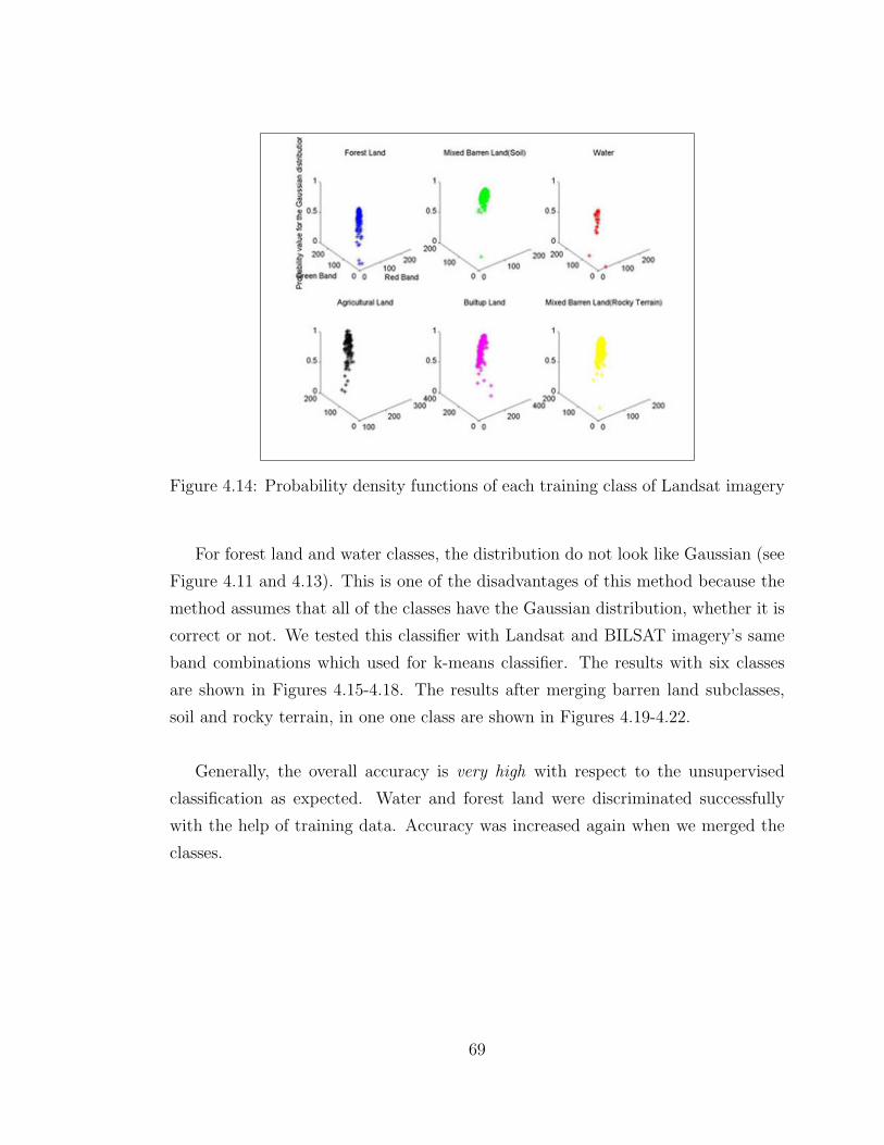
Figure 4.14: Probability density functions of each training class of Landsat imagery

For forest land and water classes, the distribution do not look like Gaussian (see

Figure 4.11 and 4.13). This is one of the disadvantages of this method because the

method assumes that all of the classes have the Gaussian distribution, whether it is

correct or not. We tested this classifier with Landsat and BILSAT imagery’s same

band combinations which used for k-means classifier. The results with six classes

are shown in Figures 4.15-4.18. The results after merging barren land subclasses,

soil and rocky terrain, in one one class are shown in Figures 4.19-4.22.

Generally, the overall accuracy is very high with respect to the unsupervised

classification as expected. Water and forest land were discriminated successfully

with the help of training data. Accuracy was increased again when we merged the

classes.

69

Figure 4.15: Classification of Landsat RGB imagery using Gaussian maximum like-lihood classifier

70

Figure 4.16: Classification of BILSAT RGB imagery using Gaussian maximum like-lihood classifier

71

Figure 4.17: Classification of Landsat RBnir imagery using Gaussian maximumlikelihood classifier

Figure 4.18: Classification of BILSAT RBnir imagery using Gaussian maximumlikelihood classifier

72

Figure 4.19: Classification of Landsat RGB imagery using Gaussian maximum like-lihood classifier

Figure 4.20: Classification of Landsat RBnir imagery using Gaussian maximumlikelihood classifier

73

Figure 4.21: Classification of BILSAT RGB imagery using Gaussian maximum like-lihood classifier

Figure 4.22: Classification of BILSAT RBnir imagery using Gaussian maximumlikelihood classifier

74

4.3 Boolean Discriminant Function Classifier

In this study, a very simple implementation of Boolean discriminant function

with seven threshold levels was considered and tested as a supervised classification.

We used threshold levels and determined the Boolean functions according to these

threshold levels which were acquired from the training data. The training data used

for this classification method is the same with the Gaussian maximum likelihood

classifier.

This method does not need a priori information or assumptions on the distribu-

tions of data. The classification results for six classes are shown in Figures 4.23 -

4.26, and for five classes, results are shown in Figures 4.27 - 4.30.

Seven threshold levels were selected for the pioneering work. Generally, solutions

with seven threshold levels of this method are not as satisfactory as the Gaussian

MLC. This method is open to the further developments. The results are sensitive to

selection of thresholds and training data. Since the approach does not include too

many priori assumptions, adaptive methods to select the parameters appropriately

can be developed based on our pioneering contribution.

The number thresholds for each band determines the radiometric resolution of

this method and it is highly distinctive on the performance. For an exaggerated

number of threshold levels much better results are possible. In Figure 4.31, an almost

perfect result for a limited region achieved by using approximately 100 threshold

levels is shown. However, the computational costs of too many thresholds for a

large image is not reasonable. The computation time when a very high number

of thresholds are used is not only affected with the number of operations, but the

data needed to be kept on RAM also increase and the computer starts to work with

virtual memory which dramatically increases the unit time per operation. Therefore,

some additional procedures to select the optimum threshold levels can improve the

overall efficiency.

75

Figure 4.23: Classification of Landsat RGB imagery using Boolean discriminantfunction classifier

76

Figure 4.24: Classification of BILSAT RGB imagery using Boolean discriminantfunction classifier

77

Figure 4.25: Classification of Landsat RBnir imagery using Boolean discriminantfunction classifier

Figure 4.26: Classification of BILSAT RBnir imagery using Boolean discriminantfunction classifier

78

Figure 4.27: Classification of Landsat RGB imagery using Boolean discriminantfunction classifier

Figure 4.28: Classification of Landsat RBnir imagery using Boolean discriminantfunction classifier

79

Figure 4.29: Classification of BILSAT RGB imagery using Boolean discriminantfunction classifier

Figure 4.30: Classification of BILSAT RBnir imagery using Boolean discriminantfunction classifier

80

Figure 4.31: Classification with Boolean discriminant function using 100 thresholdlevels

4.4 Comparision of Methods

Table 4.1 and 4.2 show the CPU time for each classifer. K-means algorithm

CPU time is affected from the initial mean values. 26sec is the average CPU time

for k-means, but the program ended with 130sec for some initial values. During

classification with Boolean discriminant function, the process for discriminating the

pixels that are assigned more than one classes has much CPU time. Table 4.2 - 4.14

show the error matrices for each classifier. When comparing these three methods,

several criteria were considered. The k-means algorithm was the fastest but had the

lowest accuracy. In the case of limited information about the study area, k-means

method can be used. This method works well also in large datasets. Maximum like-

lihood method had the highest accuracy. Boolean discriminant function results were

sufficient for the beginning. Moreover, the accuracies of MLC and BDF classifica-

tions depend strongly on the accuracy and the consistency of the provided training

sets [51].

Although BILSAT has higher spatial resolution than Landsat, its classification

results were worse than Landsat because of the radiometric characteristics. Since

in this study, only spectral reflectance was considered in the classification, here, the

81

results are directly related with the radiometric characteristics of each image.

Table 4.1: CPU time for each classifier using Landsat-7 RGB image.

Classifier CPU Time usingLandsat image (430× 281 pixels)

K-means 26secGaussian MLC 41sec

Boolean Classifier 40sec

Table 4.2: CPU time for each classifier using BILSAT RGB image.

Classifier CPU Time usingBILSAT image(456× 309 pixels)

K-means 27secGaussian MLC 47sec

Boolean Classifier 51sec

82

Table 4.3: Error matrix of classification results of Landsat RGB imagery with K-means classifier (six class).*

RDCD B R A S F W RT UAB 120 0 34 0 0 0 154 77,92%R 3 113 155 24 0 0 295 38,31%A 24 4 136 0 0 0 164 82,93%S 1 267 2 413 65 5 753 54,85%F 1 19 1 0 581 633 1235 47,04%W 0 0 0 0 0 0 0 00,00%CT 149 403 328 437 646 638 2601PA 80,54% 28,04% 41,46% 94,51% 89,94% 00,00%OA 52,40%OK 0,41

Table 4.4: Error matrix of classification results of Landsat RGB imagery with K-means classifier (five class).*

RDCD B A MB F W RT UAB 120 34 0 0 0 154 77,92%A 24 136 4 0 0 164 82,93%MB 4 157 817 65 5 1048 77,96%F 1 1 19 581 633 1235 47,04%W 0 0 0 0 0 0 00,00%CT 149 328 840 646 638 2601PA 80,54% 41,46% 97,26% 89,94% 00,00%OA 63,59%OK 0,51

*RD: Reference Data, CD: Classified Data, B: Built-up, R: Rocky terrain, A:

Agriculture, S: Soil, F: Forest land, W: Water, RT: Row Total, CT: Column Total,

PA: Producer’s Accuracy, UA: User’s Accuracy, OA: Overall classification Accuracy,

OK: Overall Kappa Statistics).

83

Table 4.5: Error matrix of classification results of BILSAT RGB imagery with K-means classifier (six class).*


Table 4.6: Error matrix of classification results of BILSAT RGB imagery with K-means classifier (five class).*






84

Table 4.7: Error matrix of classification results of Landsat RGB imagery with max-imum likelihood classifier (six class).*


Table 4.8: Error matrix of classification results of Landsat RGB imagery with max-imum likelihood classifier (five class).*






85

Table 4.9: Error matrix of classification results of BILSAT RGB imagery with max-imum likelihood classifier (six class).*


Table 4.10: Error matrix of classification results of BILSAT RGB imagery withmaximum likelihood classifier (five class).*






86

Table 4.11: Error matrix of classification results of Landsat RGB imagery withBoolean discriminant function (six class).*


Table 4.12: Error matrix of classification results of Landsat RGB imagery withBoolean Discriminant Function (five class).*






87

Table 4.13: Error matrix of classification results of BILSAT RGB imagery withBoolean discriminant function (six class).*


Table 4.14: Error matrix of classification results of BILSAT RGB imagery withBoolean discriminant function (five class).*






88

chapter 5

CONCLUSION AND

DISCUSSIONS

Remote sensing is a very complex system resulted in so many possible errors

during transferring information from one subsystem to another. They might be

originated from acquisition such as geometric aspects, sensor systems, platforms,

ground control, scene considerations; data processing such as geometric rectification,

radiometric rectification; data analysis such as quantitative analysis, classification

system, data generalization, data conversion and error assessment. Most research

work in remote sensing is aimed at minimizing these errors. In this study, efficiency

of the classification process was the main concern.

The general classification problem was pointed out from the perspective of remote

sensing. Three land cover classification techniques have been presented and imple-

mented on Landsat-7 ETM+ imagery and BILSAT imagery: K-means algorithm

and Gaussian maximum likelihood methods are well-known methods for unsuper-

vised and supervised methods. The third one is the classification by using threshold

decomposition and Boolean discriminant functions which is developed in this study.

Implementation was performed with algorithms written in MATLAB.

BILSAT’s images performance was tested and compared with Landsat-7. Al-

though BILSAT has higher spatial resolution (27m), the classification results were

better with the Landsat-7 imagery which has 30m spatial resolution. Here, the

reason is BILSAT’s images radiometric characteristics.

Six classes which are built-up, rocky terrain, soil, forest land, agriculture and

water, were selected from METU settlement with the help of field study, high res-

olution satelite image from IKONOS and air photo. According to these classes,

classification was performed and an error matrix was calculated with three meth-

89

ods. In general, k-means overall classification accuracy is 50%, maximum likelihood

has 78% accuracy and Boolean discriminant function has 65% accuracy. When two

kinds of barren land classes were combined in one class as a mixture barren land, the

accuracies increased: k-means has 60% accuracy, maximum likelihood has 85% and

boolean has 70% accuracy. From the results, maximum likelihood is the best one;

but not open to further development, and it bases on an assumption which might

not be real for another training set. On the other hand, Boolean classifier is open

to improvements and some other features such as secondary measurements derived

from the image to the feature space can be incorporated. It can be concluded that

K-means is useful when there is not enough information about the study area.

CPU time for all classifiers was calculated. The fastest algorithm is k-means

classifier. The time depends on the initial mean values. Choosing initial values far

way from the exact cluster means resulted with high CPU time. Boolean classifier

CPU time is better using Landsat image (430×281 pixels) than MLC. On the other

hand, MLC is better than the Boolean classifier using BILSAT image(456 × 309

pixels). CPU time for all classifiers depends on the size of the image, number of

clusters, number of features. For supervised classification methods, it is also strongly

affected from the training data set.

The use of Boolean discriminant functions will be improved in future studies.

This method might be promising, especially, when a class is formed by multiple

classes. In the study we used closest distance between the training samples and

unknown pixels. As a drawback, considering closest samples for classification is

not robust to outliers (for example, a single training sample corrupted by noise

could induce errors). However, the finiteness of the state space in this scheme can

be utilized to solve such problems. We can assume that each partition should be

connected within itself and eliminate the outliers (by morphological operations) by

checking whether a subspace containing a training sample has neighbours belonging

to the same class, and by checking the connectedness to the other parts of the

corresponding partition. In this study, a classification has been performed with

pixel considered for itself in this method. Due to the sensor characteristics, each

pixel’s information appears also in its neighborhood. Therefore, considering the

neighborhood of each pixel will increase the classification accuracy. Another possible

90

improvement to this method can come from the region growing method. Starting

from training samples, looking at neighborhood of each pixel and decision function,

each pixel can be added to one of the classes.

Now, most of the studies in classification use additional information, e.g. terrain

elevation, slope, aspect, texture and other sources of image such as radar, laser

data to increase the classification accuracy. To add one of the dominant discerning

features also can result in a better solutions for this study.

Our investigation uses threshold decomposition and Boolean discriminant func-

tion as a particular examples of the chosen approach. Many different parametric

function classes can be optimized as discriminants and new optimization methods,

e.g. non-smooth optimization [3] will future serve for further progress, together with

an extension of this pioneering contribution.

Considering the literature and this study, we conclude that selection of training

data is very important clue for classification. Training data should be determined

very carefully and various sources of information should also be incorporated if it

is possible. Furthermore, the selection of the categories has also a direct impact on

the perceived accuracy of the classification methods.

91

references

[1] Anderson, James R., Hardy, Erneste E., Roach, J.T. and Witmera, R. E., Land

use and land cover classification system for use with remote sensor data, A

revision of the land use classification system as presented in U.S. Geological

Survey Circular 671, Geological Survey Professional Paper 964.

[2] Arbel D., Cohen E., Citroen M., Blumberg D.G. and Kopeika N.S., Landsat

TM Satellite Image Restoration Using Kalman Filters, Photogrammetric Engi-

neering & Remote Sensing, 70, 1, (2004) 91-100.

[3] Bagirov, A. M., and Yearwood, J., A new nonsmooth optimization algorithm for

minimum sum-of-squares clustering problems, preprint, Centre for Informatics

and Applied Optimization, University of Ballarat, Australia, 2003.

[4] Beklioglu, Meryem, Burnak, S. Levent , and Ince, Ozlem, Benthi-planktivorous

fish-induced low water quality of lake Eymir before biomanipulation, Turk J.

Zool., 24, (2000) 315-326.

[5] Benediktsson, Jon A., Swain, P.H., and Ersoy O. K., Neural network approaches

versus statistical methods in classification of multisource remote sensing data,

IEEE Transactions on Geoscience and Remote Sensing, 28, 4, (1990) 540-552.

[6] Bischof, H., Schneider, W., and Pinz, A. J., Multispectral classification of

landsat-images using neural networks, IEEE Transactions Geoscience Remote

Sensing, 30, (1992) 482-490.

[7] Campbell, J. , Introduction to Remote Sensing, the Guilford Press, 1996.

[8] CEOS, Earth Observation Handbook, ESA, 2002.

[9] Congalton, Russell G., and Green Kass, Assessing the Accuracy of Remotely

Sensed Data : Principles and Practices, Lewis Publications, 1999.

92

[10] Cooke, Tristrom, A lower bound on the performance of the quadratic discrimi-

nant function, Journal of Multivariate Analysis, (2003) 371-383.

[11] Coyle, Edward J., Lin, Jean-Hsang, and Gabbouj, Moncef, Optimal stack

filtering and the estimation and structural approaches to image processing, IEEE

Transactions on Acoustics, Speech and Signal Processing, 37, 12, (1989) 2037-

2066.

[12] Cracknell, A.P., A Review Article, Synergy in Remote Sensing-What is in a

pixel?, International Journal of Remote Sensing, 19, 11,(1998) 2025-2047.

[13] Ediriwickrema, J., and Khorram, Siamak, Hierarchical maximum-likelihood

classifiation for improved accuracies, IEEE Transactions on Geoscience and

Remote Sensing, 35, 4, (1997) 810-816.

[14] Erdem, Nilufer, and Diri, Banu, Classification tool, senior project, report, Com-

puter Engineering Department, Yıldız Techncal University, 2005.

[15] Finnerty, Scott, and Sen, Sandip, Simulated annealing based classification,

IEEE, (1994) 824-827.

[16] Foody, Giles M., Status of land cover classification accuracy assessment, Re-

mote Sensing of Environment, (2002) 185-201.

[17] Gabbouj, Moncef, Digital Image Processing Lecture Notes, Tampere University

of Technology, 2004.

[18] Gao, Jay, Chen, Huifen, Zhang, Ying, and Zha Yong, Knowledge-based ap-

proaches to accurate mapping of mangroves from satellite data, Photogram-

metric Engineering&Remote Sensing, 70, 11, (2004) 1241-1248.

[19] Hastie, T., Tibshirani, R., and Friedman, Jerome, The Elements of Statistical

Learning, Data Mining, Inference and Prediction, Springer, 2001.

[20] Heermann, P. D., and Khazenie, N., Classification of multispectral remote sens-

ing data using a back-propagation neural network, IEEE Transactions on Geo-

science and Remote Sensing, 30, (1992) 81-88.

93

[21] Houston, A., and Rycroft, M., Keys to Space, An Interdisciplinary Approach to

Space Studies, International Space University Publication, 2003.

[22] IKONOS Product Imagery Products and Product Guide, IKONOS Space Imag-

ing, 2004.

[23] Jackson, Qiong, and Langrebe, D.A., An adaptive method for combined co-

variance estimation and classification, IEEE Transactions on Geoscience and

Remote Sensing, 40, 5, (2002) 1082-1087.

[24] Jain, A.K., Fundamentals of Digital Image Processing, University of California,

Prentice Hall Information and System Sciences Series, 1989.

[25] Jain, A.K., Murty, M. N., and Flynn, P.J., Data clustering: a review, ACM

Computing Surveys, 31, 3, (1999) 277-323.

[26] Jensen, J., Introductory Digital Image Processing, A Remote Sensing Perspec-

tive, Prentice Hall Series in Geographic Information Science, 1996.

[27] Kartikeyan, B., Majumder, K. L., and Dasgupta, A.R., An expert system for

land cover classification, IEEE Transactions on Geoscience and Remote Sens-

ing, 33, 1, (1995), 58-66.

[28] Kartikeyan, B., Sarkar, A., Majumder, K L., A segmentation approach to clas-

sification of remote sensing imagery, International Journal of Remote Sensing,

19, 9, (1998) 1695-1709.

[29] Kelly, Maggi, Shaari, David, Guo, Qinghua, and Liu, Desheng, A comparision

of standard and hybrid classifier methods for mapping hardwood mortality in

areas affected by ”sudden oak death”, Photogrammetric Engineering&Remote

Sensing, 70, 11, (2004) 1229-1239.

[30] Khorram, S., Digital Image Processing, International Space University Summer

Session Program Lecture Notes, 2003.

94

[31] Korumduk, Cumali, and Pestemalcı, Vedat, Determination of Forest Covered

Areas in the Northern of Adana City by Using Satellite Data, MSc. Thesis,

Cukurova University, 2002.

[32] Lai, Pak-Cheung, and Zeng, Bing, Fast sub-optimal design of extended threshold

Boolean filters, IEEE, (1999) 438-441.

[33] Lee, Ki Dong, and Lee, Yong Hoon, Threshold Boolen filters, IEEE Transactions

on Signal Processing, 42, 8, (1994) 2022-2036.

[34] Lillesand, T. M., and Kiefer, R. W., Remote Sensing and Image Interpretation,

University of Wisconsin, John Wiley&Sons, 2000.

[35] Liu, Weiguo, Gopal, Sucharita, and Woodcock, Curtis E., Uncertainty and

confidence in land cover classification using a hybrid classifier approach, Pho-

togrammetric Engineering&Remote Sensing, 70, 8, (2004) 963-971.

[36] Liu, Z. K., and Xiao, J. Y., Classification of remotely-sensed image data using

artificial neural networks, International Journal of Remote Sensing, 12, 11,

(1991) 2433-2438.

[37] Lu, Dengsheng, Musel, Paul, Batistella, Mteus, and Moran, Emilio, Compari-

sion of land cover classification methods in the Brazilian Amazon basin, Pho-

togrammetric Engineering&Remote Sensing, 70, 6, (2004) 723-731.

[38] Lu, Dengsheng, and Weng, Qihao, Spectral mixture analysis of the urban land-

scape in Indianapolis with Landsat ETM+ imagery, Photogrammetric Engi-

neering&Remote Sensing, 70, 9, (2004) 1053-1062.

[39] Mather, P.M., Computer Processing of Remotely Sensed Images, An Introduc-

tion, School of Geography, the University of Nottingham, UK, Wiley, 1999.

[40] Mausel, P.W., Kamber, W.J., and Lee, J.K., Optimum band selection for su-

pervised classification of multispectral data, Photogrammetric Engineering and

Remote Sensing, (1990).

95

[41] McCauley, James Darrell, and Engel, Bernard A., Communications, IEEE

Transactions on Geoscience and Remote Sensing, 33, 6, (1995) 1103-1109.

[42] Muneyasu, Mitsuji, Yasui, Yoshihiro, and Hinamoto, Takao, A design of adap-

tive stack filters using pattern classification, IEEE, (1999) 534-538.

[43] Myint, Soe Win, Lam, Nina S.-N., and Tyler, J.M., Wavelets for urban spa-

tial feature discrimination: comparisions with fractal, spatial autocorrelation,

and spatial co-occurrence approaches, Photogrammetric Engineering&Remote

Sensing, 70, 7, (2004) 1313-1316.

[44] Orun, Ahmet B., Automated Identification of Man-made textural features

on satellite imagery by Bayesian networks, Photogrammetric Engineer-

ing&Remote Sensing, 70, 2, (2004) 211-216.

[45] Pal, Mahesh, and Mather, Paul M., An assessment of the effectiveness of deci-

sion tree methods for land cover classification, Remote Sensing of Environment

86, (2003) 554-565.

[46] Paola, Justin D., and Schowengerdt, Robert A., A detailed of back propagation

neural network and maximum likelihood classifiers for urban land use classifi-

cation, IEEE Transactions on Geoscience and Remote Sensing, 33, 4, (1995)

981-996.

[47] Peter, Clote, and Kranakis, Evangelos, Boolean Functions and Computation

Models, Springer, 2001.

[48] Platt, R.V., and Goetz, A.F.H., A comparision of AVIRIS and Landsat

ETM+ land use classification at the urban area, Photogrammetric Engineer-

ing&Remote Sensing, 70, 7, (2004) 813-819.

[49] Porter, Reid, Harvey, Neal, Perkins, Simon, Theiler, James, Brumby, Steven,

Bloch, Jeff, and Gokhale, Maya Szymanski, Optimizing Digital Harware Per-

ceptrons for Multi-Spectral Image Classification.

96

[50] Punch, W.F., Goodman, E.D., Pei, Min, Chia-Sun, Lai, Hovland, P., and En-

body, R., Further Research on Feature selection and classification using genetic

algorithms, ICGA93, (1993) 557-594, Champaign 3.

[51] Salu, Yehuda, and Tilton, James, Classification of multispectral image data

by the binary diamond neural network and by nonparametric, pixel by pixel

methods, IEEE Transactions on Geoscience and Remote Sensing, 31, 3, (1993)

606-617.

[52] Schackelford, Aaron K., and Davis, Curt H., A fuzzy classification approach for

high-resolution multispectral data over urban areas, IEEE, (2002) 1621-1623.

[53] Schowengerdt, R.A., Remote Sensing, Models and Methods for Image Process-

ing, University of Arizona, Academic Press, 1997.

[54] Smiths, Paul C., Multiple classifier systems for supervised remote sensing im-

age classification based on dynamic classifier selection, IEEE Transactions on

Geoscience and Remote Sensing, 40, 4, (2002) 801-813.

[55] Tso, B., and Mather, P.M., Classification Methods for Remotely Sensed Data,

Taylor and Francis, London and New York, 2001.

[56] Usul, Nurunnisa, and Doganoglu, Veysel, METU Land and Campus in GIS,

METU project supported by DPT.

[57] Visual Interpretation of Images with the Help of Colour Composites: Getting

to Know the Study Area, ISU Lecture Notes, 2003.

[58] Walter, Volker, Object based classification of remote sensing data for change

detection, ISPRS Journal of Photogrammetry and Remote Sensing, 58, (2004)

225-238.

[59] Wang, Ywqiao, and Zhang, Xinsheng, A SPLIT model for extraction of sub-

pixel impervious surface information, Photogrammetric Engineering&Remote

Sensing, 70, 7, (2004) 821-828.

97

[60] Wilkinson, Graeme G., Results and implications of a study of fifteen years of

satellite image classifications experiments, IEEE Transactions on Geoscience

and Remote Sensing, 43, 3, (2005) 433-440.

[61] Yang, Limin, Huang, Chengquan, Homer, Collin H., Wylie, B.K., and Coan,

Micheal J., An approach for mapping large-area impervious surfaces: synergis-

tic use of Landsat 7 ETM+ and high spatial resolution imagery, manuscript

submitted to Canadian Journal of Remote Sensing (research paper), (2002)

USGS.

[62] Yoshida, Tomoji, and Sigeru, Omatu, Neural network approcah to land cover

mapping, IEEE Transactions on Geoscience and Remote Sensing, 32, 5, (1994)

1103-1109.

[63] Yuksel, Gokhan et al., BILSAT-1: first year in orbit-operations and lessons

learned, the 18th Annual AIAA/USU Conference on Small Satellites, (2004).

[64] Zavaljevski, Aleksandar, Classification and Detection in Multispectral Images,

PhD thesis in Electrical Engineering, University of Cincinnati, 1996.

[65] Zhu, Changqing, and Yang, Xiaomei, Study of remote sensing image texture

analysis and classification using wavelet, International Journal of Remote Sens-

ing, 19, 16, (1998) 3197-3203.

[66] Airborne Remote Sensing Basics

http://hydrolab.arsusda.gov/rsbasics/noise.php (accessed 06 Sep. 2005).

[67] Electromagnetic spectrum From Wikipedia, the free encyclopedia.

http://en.wikipedia.org/wiki/Electromagnetic-spectrum (accessed 06 Sep.

2005).

[68] Fundamentals of Remote Sensing, Remote Sensing Tutorial, Canada Centre for

Remote Sensing, Natural Resources, Canada

http://www.ccrs.nrcan.gc.ca/ccrs/homepg.pl?e (accessed 06 Sep. 2005).

[69] Google Earth

http://earth.google.com/ (accessed 06 Sep. 2005).

98

[70] Hyperspectral Remote Sensing Systems and Analysis Glenn J. Fitzgerald,

Ph.D. USDA-ARS, Shafter, CA

http://webpages.acs.ttu.edu/smaas/asa2000/fitzgerald.htm (accessed 06 Sep.

2005).

[71] Landsat-7 Science Data User’s Handbook

http://ltpwww.gsfc.nasa.gov/IAS/handbook/handbook toc.html (accessed 06

Sep. 2005).

[72] Middle East Technical University homepage

www.metu.edu.tr (accessed 06 Sep. 2005).

99

APPENDIXA

FILE booleanthresh.m

% (C) Selime Gurol (September, 2005)

function bcindsson = booleanthresh(A, n, v1, v2, v3, v4, v5, v6)

% A is the input matrix.

% n is the number of classes

% bcindsson matrix is the output whose elements valued from 1 to 6. If the user

% represents the numbers with colours, thematic map is appeared on the screen.

% v1, v2, v3, v4, v5, v6 are the training data for each class. These training data

% are selected with trainselection.m file.

% v1 represents training data for water

% v2 represents training data for forest

% v4 represents training data for rock

% v5 represents training data for agriculture

% v6 represents training data for builtup

tic;

% Determination of RGB and mean values for each training data set with an

% order.

[r1, g1, b1, a] = trainsort(v1);

[r2, g2, b2, b] = trainsort(v2);

[r3, g3, b3, c] = trainsort(v3);

[r4, g4, b4, d] = trainsort(v4);

[r5, g5, b5, e] = trainsort(v5);

[r6, g6, b6, f ] = trainsort(v6);

100

% Selection of threshold levels to be used for threshold decomposition

TR = [0.5∗ (f(1)+250) 0.5∗ (f(1)+ e(1)) 0.5∗ (e(1)+d(1)) 0.5∗ (d(1)+ c(1))

0.5 ∗ (c(1) + b(1)) 0.5 ∗ (b(1) + a(1)) 0.5 ∗ a(1)]

TG = [0.5∗ (f(2)+250) 0.5∗ (f(2)+ e(2)) 0.5∗ (e(2)+d(2)) 0.5∗ (d(2)+ c(2))

0.5 ∗ (c(2) + b(2)) 0.5 ∗ (b(2) + a(2)) 0.5 ∗ a(2)]

TB = [0.5∗ (f(3)+250) 0.5∗ (f(3)+ e(3)) 0.5∗ (e(3)+d(3)) 0.5∗ (d(3)+ c(3))

0.5 ∗ (c(3) + b(3)) 0.5 ∗ (b(3) + a(3)) 0.5 ∗ a(3)]

% Threshold Decomposition of the input image according to the TR, TG and

% TB threshold vectors and remaining feature values

[rbv, rcv, gbv, gcv, bbv] = thrdecom(A, TR, TG, TB);

% Assignment of each pixel to the classes

[bcinds1, nonind1] = solution(v1, r1, g1, b1, TR, TG, TB, rbv, rcv, gbv, gcv, bbv);






bcinds(:, :, 1) = bcinds1;






[x, y] = size(A(:, :, 1));

son mat = bcinds1 + bcinds2 + bcinds3 + bcinds4 + bcinds5 + bcinds6;

t1=toc

tic

for i = 1 : x

101

for j = 1 : y

son = son mat(i, j);

if son == 1;

bcindsson(i, j) = find(bcinds(i, j, :) == 1);

% Assignment of pixels that are assigned more than one classes

elseif son > 1

K(1, :) = rbv(i, j, :);

K(2, :) = gbv(i, j, :);

K(3, :) = bbv(i, j, :);

KK(1, :) = rcv(i, j, 1);

KK(2, :) = rcv(i, j, 2);

KK(3, :) = gcv(i, j, 1);

KK(4, :) = gcv(i, j, 2);

indis=find(bcinds(i, j, :) == 1);

comp= [a; b; c; d; e; f ];

for k = 1 : length(indis)

meant = comp(indis(k), :);

L(1, :, k) = meant(1) > TR;

L(2, :, k) = meant(2) > TG;

L(3, :, k) = meant(3) > TB;

LL(1, :, k) = meant(1) > min(A(i, j, 2), A(i, j, 3));

LL(2, :, k) = meant(1) > max(A(i, j, 2), A(i, j, 3));

LL(3, :, k) = meant(2) > min(A(i, j, 1), A(i, j, 3));

LL(4, :, k) = meant(2) > max(A(i, j, 1), A(i, j, 3));

SUM1(k) = sum(sum(K == L(:, :, k)));

SUM2(k) = sum(sum(KK == LL(:, :, k)));

SUM(k) = SUM1(k) + SUM2(k);

end

location = find(SUM == max(SUM));

bcindsson(i, j) = indis(location(1));

clear location

clear SUM

102

% Assignment of unclassified pixels

else

D = [nonind1, nonind2, nonind3, nonind4, nonind5, nonind6];

DDD = find(D == max(D));

bcindsson(i, j) = DDD(1);

end

clear LLL

end

end

t2=toc

%%%%%%%%%%%%%%%%%SUBFUNCTIONS%%%%%%%%%%%%%

function [rout, gout, bout,meantrain] = trainsort(vin)

% vin is the training data set

% The outputs rout, gout, bout are red band, green band and

% blue band values with an order for the corresponding training set

% meantrain is a 3D vector whose elements are the mean values of RGB

% bands of corresponding training data set

vpro = sort(vin);

vpro = vpro(2 : length(vpro)− 1, :);

meantrain = mean(vpro);

rout = vpro(:, 1);

gout = vpro(:, 2);

bout = vpro(:, 3);

%%%%%%%%%%%%%%%%%%%%%%%%%%%%%%%%%%%%%%%%

function [rbv, rcv, gbv, gcv, bbv] = thrdecom(A, TR, TG, TB);

% inputs are an image 3D-matrice and 3 vectors of thresholds for each band

% outputs are 3D matrices of Boolean vectors

sizeimg = size(A);

sizered = length(TR);

sizegreen = length(TG);

103

sizeblue = length(TB);

rbv = zeros(sizeimg(1), sizeimg(2), sizered);

rcv = zeros(sizeimg(1), sizeimg(2), 2);

gbv = zeros(sizeimg(1), sizeimg(2), sizegreen);

gcv = zeros(sizeimg(1), sizeimg(2), 2);

bbv = zeros(sizeimg(1), sizeimg(2), sizeblue);

for i = 1 : sizered

rbv(:, :, i) = A(:, :, 1) > TR(i);

end

rcv(:, :, 1) = A(:, :, 1) > min(A(:, :, 2), A(:, :, 3));

rcv(:, :, 2) = A(:, :, 1) > max(A(:, :, 2), A(:, :, 3));

for i = 1 : sizegreen,

gbv(:, :, i) = A(:, :, 2) > TG(i);

end

gcv(:, :, 1) = A(:, :, 2) > min(A(:, :, 1), A(:, :, 3));

gcv(:, :, 2) = A(:, :, 2) > max(A(:, :, 1), A(:, :, 3));

for i = 1 : sizeblue,

bbv(:, :, i) = A(:, :, 3) > TB(i);

end

%%%%%%%%%%%%%%%%%%%%%%%%%%%%%%%%%%%%%%%%

function [bcindsout, nonindout] = solution(vin, rin, gin, bin, TR, TG, TB, rbv,

rcv, gbv, gcv, bbv)

% solution.m is a function that assigns the pixels to the classes.

% Threshold Decomposition of the training data set according to the TR,

% TG and TB threshold vectors and remaining feature min, max values.

[samplesrb, samplesrc, samplesgb, samplesgc, samplesbb] =

fullthresdec(vin, rin, gin, bin, TR, TG, TB);

% Determination of the indicator to a Boolean classifier function which uniquely

% discriminates the dataset

104

indfunindcls = infunfin(samplesrb, samplesrc, samplesgb, samplesgc, samplesbb);

[bcinds, nonind] = bccheck(rbv, rcv, gbv, gcv, bbv, indfunindcls);

bcindsout = bcinds;

nonindout = nonind;

%%%%%%%%%%%%%%%%%%%%%%%%%%%%%%%%%%%%%%%%

function [samplesrb, samplesrc, samplesgb, samplesgc, samplesbb] =

fullthresdec(vin, rband, gband, bband, TR, TG, TB)

% Threshold Decomposition of rband

[samplesrb, samplesrc] = thresdec(vin, rband, gband, bband, TR);

% Threshold Decomposition of gband

[samplesgb, samplesgc] = thresdec(vin, gband, rband, bband, TG);

% Threshold Decomposition of bband according to the TB threshold vector

for i = 1 : length(vin)− 2

for k = 1 : length(TR)

samplesbb(i, k) = bband(i) > TB(k);

end

end

%%%%%%%%%%%%%%%%%%%%%%%%%%%%%%%%%%%%%%%%

function[samplesband1, samplesband1comp] = thresdec(vin, band1, band2,

band3, T IN)

% samplesband1 is a matrix that its ith column is a Boolean vector obtained

% from threshold decomposition of band1 according to the TIN(i) threshold

% level (i = 1, 2, ..., length(TIN))

% sampleband1comp columns are the Boolean vectors obtained from the

% threshold decomposition according to the min, max values of band2 and band3.


105

for k = 1 : length(TIN)

samplesband1(i, k) = band1(i) > TIN(k);

end

end


samplesband1comp(i, length(TIN)+1) = band1(i) > min(band2(i), band3(i));

samplesband1comp(i, length(TIN)+2) = band1(i) > max(band2(i), band3(i));

end

%%%%%%%%%%%%%%%%%%%%%%%%%%%%%%%%%%%%%%%%

function indfunindcls =

infunfin(samplesrb, samplesrc, samplesgb, samplesgc, samplesbb);

% input is the samples known to belong to the same class (training samples of

%a class)

% it is a set of matrices of boolean vectors

% output is an indicator to a Boolean classifier function which uniquely

% discriminates the dataset

sizzr = size(samplesrb);

sizzg = size(samplesgb);

sizzb = size(samplesbb);

nofsamples = sizzr(1);

indfunindcls = [sum(samplesrb(1, :)), sum(samplesrc(1, :)),

sum(samplesgb(1, :)), sum(samplesgc(1, :)), sum(samplesbb(1, :))];

k = 1;

for i = 2 : nofsamples

indfunindclse = [sum(samplesrb(i, :)), sum(samplesrc(i, :)),

sum(samplesgb(i, :)), sum(samplesgc(i, :)), sum(samplesbb(i, :))];

lll = sum(indfunindcls(1, :) == indfunindclse);

for j = 1 : k,

lll = max(lll, sum(indfunindcls(k, :) == indfunindclse));

end

if lll < 5

indfunindcls = [indfunindcls; indfunindclse];

106

k = k + 1;

end

end

%%%%%%%%%%%%%%%%%%%%%%%%%%%%%%%%%%%%%%%%

function [bcinds, nonind] = bccheck(rbv, rcv, gbv, gcv, bbv, indfunindcls);

% checks which pixels on an image belong to the corresponding class

% inputs are the threshold decompositon vectors

% output is a binary matrix

sizind = size(indfunindcls);

nofors = sizind(1);

summ1 = sum(rbv, 3);

summ2 = sum(rcv, 3);

summ3 = sum(gbv, 3);

summ4 = sum(gcv, 3);

summ5 = sum(bbv, 3);

indic = zeros(size(summ1));

unclassifiedtotal = 0;

unclassifiedtotal1 = 0;





for i = 1 : nofors

ind1 = (summ1 == indfunindcls(i, 1));





indik = ind1. ∗ ind2. ∗ ind3. ∗ ind4. ∗ ind5;

indic = indic + indik;

end

nonind = sum(sum(ind1)) + sum(sum(ind2)) + sum(sum(ind3))+

107

sum(sum(ind4)) + sum(sum(ind5));

bcinds = indic > 0.1;

108

APPENDIXB

BILSAT IMAGE OF

METU SETTLEMENT

109

APPENDIXC

LANDSAT IMAGE OF

METU SETTLEMENT

110

statistical learning and optimization …statistical learning and optimization methods for ......

Documents