StatisticalMechanicsProblemswithsolutions

KonstantinKLikharev

IOPPublishing,Bristol,UK

©CopyrightKonstantinKLikharev2019

All rights reserved. No part of this publication may be reproduced, stored in a retrieval system ortransmitted in any form or by any means, electronic, mechanical, photocopying, recording or otherwise,withoutthepriorpermissionofthepublisher,orasexpresslypermittedbylaworundertermsagreedwiththeappropriaterightsorganization.Multiplecopyingispermittedinaccordancewiththetermsoflicencesissuedby theCopyright LicensingAgency, theCopyrightClearanceCentre and other reproduction rightsorganizations.

Permission to make use of IOP Publishing content other than as set out above may be sought atpermissions@ioppublishing.org.

KonstantinKLikharevhasassertedhisrighttobeidentifiedastheauthorofthisworkinaccordancewithsections77and78oftheCopyright,DesignsandPatentsAct1988.

ISBN978-0-7503-1419-0(ebook)ISBN978-0-7503-1420-6(print)ISBN978-0-7503-1421-3(mobi)

DOI10.1088/2053-2563/aaf504

Version:20190701

IOPExpandingPhysicsISSN2053-2563(online)ISSN2054-7315(print)

BritishLibraryCataloguing-in-PublicationData:AcataloguerecordforthisbookisavailablefromtheBritishLibrary.

PublishedbyIOPPublishing,whollyownedbyTheInstituteofPhysics,London

IOPPublishing,TempleCircus,TempleWay,Bristol,BS16HG,UK

USOffice:IOPPublishing,Inc.,190NorthIndependenceMallWest,Suite601,Philadelphia,PA19106,USA

ContentsPrefacetotheEAPSeriesPrefacetoSMProblemswithSolutionsAcknowledgmentsNotation

1 ReviewofthermodynamicsReferences

2 PrinciplesofphysicalstatisticsReferences

3 Idealandnot-so-idealgasesReferences

4 Phasetransitions

5 FluctuationsReferences

6 ElementsofkineticsReferences

Appendices

A Selectedmathematicalformulas

B Selectedphysicalconstants

Bibliography

PrefacetotheEAPSeries

EssentialAdvancedPhysicsEssentialAdvancedPhysics(EAP)isaseriesoflecturenotesandproblemswithsolutions,consistingofthefollowingfourparts1:

PartCM:ClassicalMechanics(aone-semestercourse),PartEM:ClassicalElectrodynamics(twosemesters),PartQM:QuantumMechanics(twosemesters),andPartSM:StatisticalMechanics(onesemester).

Eachpart includestwovolumes:LectureNotesandProblemswithSolutions,andanadditional

fileTestProblemswithSolutions.

Distinguishingfeaturesofthisseries—inbriefcondensedlecturenotes(∼250pppersemester)—muchshorterthanmosttextbooksemphasisonsimpleexplanationsofthemainnotionsandphenomenaofphysicsafocusonproblemsolution;extensivesetsofproblemswithdetailedmodelsolutionsadditionalfileswithtestproblems,freelyavailabletoqualifieduniversityinstructorsextensivecross-referencingbetweenallpartsoftheseries,whichsharestyleandnotation

LevelandprerequisitesThe goal of this series is to bring the reader to a general physics knowledge level necessary forprofessional work in the field, regardless on whether the work is theoretical or experimental,fundamentalorapplied.Fromtheformalpointofview,thislevel(augmentedbyafewspecialtopiccourses in a particular field of concentration, and of course by an extensive thesis researchexperience)satisfiesthetypicalPhDdegreerequirements.Selectedpartsoftheseriesmaybealsovaluableforgraduatestudentsandresearchersofotherdisciplines,includingastronomy,chemistry,mechanicalengineering,electrical,computerandelectronicengineering,andmaterialscience.TheentrylevelisanotchlowerthanthatexpectedfromaphysicsgraduatefromanaverageUS

college. Inaddition tophysics, theseriesassumes thereader’s familiaritywithbasiccalculusandvectoralgebra, tosuchanextentthat themeaningof the formulas listed inappendixA,‘Selectedmathematicalformulas’(reproducedattheendofeachvolume),isabsolutelyclear.

OriginsandmotivationTheseriesisaby-productoftheso-called‘corephysicscourses’ItaughtatStonyBrookUniversityfrom1991to2013.Mymaineffortwastoassistthedevelopmentofstudents’problem-solvingskills,ratherthantheiridlememorizationofformulas.(Withacertainexaggeration,mylectureswerenotmuchmorethanintroductionstoproblemsolution.)Thefocusonthismainobjective,undertherigidtime restrictions imposed by the SBU curriculum, had some negatives. First, the list of coveredtheoreticalmethodshadtobelimitedtothosenecessaryforthesolutionoftheproblemsIhadtimeto discuss. Second, I had no time to cover some core fields of physics—most painfully generalrelativity2andquantumfieldtheory,beyondafewquantumelectrodynamicselementsattheendofPartQM.Themainmotivationforputtingmylecturenotesandproblemsonpaper,andtheirdistributionto

students,wasmy desperation to find textbooks and problem collections I could use,with a clearconscience, formy purposes. The available graduate textbooks, including the famousTheoreticalPhysics series by Landau andLifshitz, did notmatch theminimalistic goal ofmy courses,mostlybecause they are far too long, and using them would mean hopping from one topic to another,pickingupa chapterhereanda section there, at ahigh riskof losing thenecessarybackgroundmaterialand logicalconnectionsbetween thecoursecomponents—and thestudents’ interestwiththem. In addition, many textbooks lack even brief discussions of several traditional and moderntopicsthatIbelievearenecessarypartsofeveryprofessionalphysicist’seducation3.On theproblemside,mostavailablecollectionsarenotbasedonparticular textbooks,and the

problem solutions in them either do not refer to any backgroundmaterial at all, or refer to theincludedshortsetsofformulas,whichcanhardlybeusedforsystematiclearning.Also,thesolutionsarefrequentlytooshorttobeuseful,andlackdiscussionsoftheresults’physics.

StyleInanefforttocomplywiththeOccam’sRazorprinciple4,andbeatMalek’slaw5,Ihavemadeeveryefforttomakethediscussionofeachtopicasclearasthetime/space(andmyability:-)permitted,andassimpleasthesubjectallowed.Thisefforthasresultedinrathersuccinctlecturenotes,whichmaybethoroughlyreadbyastudentduringthesemester.Despitethisbriefness,theintroductionofeverynewphysicalnotion/effectandofeverynoveltheoreticalapproachisalwaysaccompaniedbyanapplicationexampleortwo.Theadditionalexercises/problemslistedattheendofeachchapterwerecarefullyselected6,so

thattheirsolutionscouldbetterillustrateandenhancethelecturematerial.Informalclasses,theseproblemsmaybeusedforhomework,whileindividuallearnersarestronglyencouragedtosolveasmanyof themaspracticallypossible.The fewproblemsthatrequireeither longercalculations,ormorecreativeapproaches(orboth),aremarkedbyasterisks.Incontrastwiththelecturenotes,themodelsolutionsoftheproblems(publishedinaseparate

volume for eachpart of the series) aremoredetailed than inmost collections. In some instancestheydescribeseveralalternativeapproachestotheproblem,andfrequentlyincludediscussionsofthe results’ physics, thus augmenting the lecture notes. Additional files with sets of shorterproblems (also with model solutions) more suitable for tests/exams, are available for qualifieduniversityinstructorsfromthepublisher,freeofcharge.

DisclaimerandencouragementThe prospective reader/instructor has to recognize the limited scope of this series (hence thequalifierEssentialinitstitle),andinparticularthelackofdiscussionofseveraltechniquesusedincurrenttheoreticalphysicsresearch.Ontheotherhand,Ibelievethattheseriesgivesareasonableintroduction to the hard core of physics—which many other sciences lack. With this hard coreknowledge, today’s student will always feel at home in physics, even in the often-unavoidablesituations when research topics have to be changed at a career midpoint (when learning fromscratch is terribly difficult—believe me :-). In addition, I have made every attempt to reveal theremarkablelogicwithwhichthebasicnotionsandideasofphysicssubfieldsmergeintoawonderfulsingleconstruct.MoststudentsItaughtlikedusingmymaterials,soIfancytheymaybeusefultoothersaswell—

hencethispublication,forwhichalltextshavebeencarefullyreviewed.

1Note that the (very ambiguous) termmechanics is used in these titles in its broadest sense. The acronymEM stems from another popular name for classicalelectrodynamicscourses:ElectricityandMagnetism.2Foranintroductiontothissubject,IcanrecommendeitherabriefreviewbySCarroll,SpacetimeandGeometry(2003,NewYork:Addison-Wesley)oralongertextbyAZee,EinsteinGravityinaNutshell(2013,PrincetonUniversityPress).3To list just a few: the statics and dynamics of elastic and fluid continua, the basics of physical kinetics, turbulence and deterministic chaos, the physics ofcomputation,theenergyrelaxationanddephasinginopenquantumsystems,thereduced/RWAequationsinclassicalandquantummechanics,thephysicsofelectronsand holes in semiconductors, optical fiber electrodynamics, macroscopic quantum effects in Bose–Einstein condensates, Bloch oscillations and Landau–Zenertunneling,cavityquantumelectrodynamics,anddensityfunctionaltheory(DFT).Allthesetopicsarediscussed,ifonlybriefly,inmylecturenotes.4Entianonsuntmultiplicandapraeternecessitate—Latinfor‘Donotusemoreentitiesthannecessary’.5‘Anysimpleideawillbewordedinthemostcomplicatedway’.6Manyoftheproblemsareoriginal,butitwouldbesillytoavoidsomeoldgoodproblemideas,withlong-lostauthorship,whichwanderfromonetextbook/collectiontoanotheronewithoutreferences.Theassignmentsandmodelsolutionsofallsuchproblemshavebeenre-workedcarefullytofitmylecturematerialandstyle.

PrefacetoSMProblemswithSolutionsThis volume of the EAP series containsmodel solutions of the problems formulated in volume 7,Statistical Mechanics: Lecture Notes. For reader’s convenience, the problem assignments arereproducedinthisvolumeaswell,althoughtheaccompanyingfiguresarefrequentlymoredetailed,extended to explain the solutions. The appendices A (Selected mathematical formulas) and B(Selectedphysicalconstants),commonforallpartsoftheseries,arealsoincludedinthisvolume.

Since the whole series is strongly focused on the development of problem solution skills, themodelsolutionsareratherdetailed,andinsomecases(particularlyinthemoredifficultproblems,markedbyasterisks)extendand/orenhancethelecturematerial.

Numberingofformulaswithineachsolutionislocal,byasterisks;referencestoformulasinothersolutions are clearly indicated. The solutions also have numerous references to formulas in thelecturenotesofthis(SM)partoftheEAPseries,andoccasionallythoseinotherpartsoftheseries.Inthelattercase,theacronymofthepartisincludedintothereference.

A file with 25 additional problems, which allow shorter solutions and hence are suitable forexams (also with model solutions) is available to university instructors from the publisher byrequest.

Theauthortriedhardtoeliminateallerrorsinthesolutions,buttheyhavenotpassedarigorousreviewbyqualifiedothers,andarepresentedherewithoutwarranty.

AcknowledgmentsIamextremelygratefultomyfacultycolleaguesandotherreadersofthepreliminary(circa2013)versionofthisseries,whoprovidedfeedbackoncertainsections;heretheyarelistedinalphabeticalorder7:AAbanov,PAllen,DAverin,SBerkovich,P-TdeBoer,MFernandez-Serra,RFHernandez,AKorotkov,VSemenov,FSheldon,andXWang.(Obviously,thesekindpeoplearenotresponsibleforanyremainingdeficiencies.)

Alargepartofmyscientificbackgroundandexperience,reflectedinthesematerials,camefrommy education, and then research, in theDepartment of Physics ofMoscowStateUniversity from1960 to 1990. The Department of Physics and Astronomy of Stony Brook University provided acomfortableandfriendlyenvironmentformyworkduringthefollowing25+years.

Lastbutnotleast,IwouldliketothankmywifeLioudmilaforallherlove,care,andpatience—withoutthese,thiswritingprojectwouldhavebeenimpossible.

I know very well that my materials are still far from perfection. In particular, my choice ofcoveredtopics(alwaysverysubjective)maycertainlybequestioned.Also, it isalmostcertainthatdespiteallmyefforts,notalltyposhavebeenweededout.Thisiswhyallremarks(howevercandid)and suggestions from readers will be greatly appreciated. All significant contributions will begratefullyacknowledgedinfutureeditions.

KonstantinKLikharevStonyBrook,NY

7IamverysorryfornotkeepingproperrecordsfromthebeginningofmylecturesatStonyBrook,soIcannotlistallthenumerousstudentsandTAswhohavekindlyattractedmyattentiontotyposinearlierversionsofthesenotes.Needlesstosay,Iamverygratefultoallofthemaswell.

Notation

Abbreviations Fonts Symbols

c.c.complexconjugate F, scalarvariables8 .timedifferentiationoperator(d/dt)

h.c.Hermitianconjugate F, vectorvariables ∇spatialdifferentiationvector(del)

scalaroperators ≈approximatelyequalto

vectoroperators ∼ofthesameorderas

Fmatrix ∝proportionalto

Fjj′matrixelement ≡equaltobydefinition(orevidently)

⋅scalar(‘dot-’)product

×vector(‘cross-’)product__timeaveraging

⟨⟩statisticalaveraging

[,]commutator

{,}anticommutator

PrimesignsTheprimesigns(′,″,etc)areusedtodistinguishsimilarvariablesorindices(suchasjandj′inthematrixelementabove),ratherthantodenotederivatives.

PartsoftheseriesPartCM:ClassicalMechanics  PartEM:ClassicalElectrodynamicsPartQM:QuantumMechanics  PartSM:StatisticalMechanics

AppendicesAppendixA:SelectedmathematicalformulasAppendixB:Selectedphysicalconstants

FormulasTheabbreviationEq.maymeananydisplayedformula:eithertheequality,orinequality,orequation,etc.

8Thesameletter,typesetindifferentfonts,typicallydenotesdifferentvariables.

(*)

IOPPublishing

StatisticalMechanicsProblemswithsolutionsKonstantinKLikharev

Chapter1

Reviewofthermodynamics

Problem1.1.Twobodies,with temperature-independentheatcapacitiesC1andC2, anddifferentinitialtemperaturesT1andT2,areplacedintoaweakthermalcontact.Calculatethechangeofthetotalentropyofthesystembeforeitreachesthethermalequilibrium.

Solution:Duetothethermalcontactweakness,eachbodyisclosetointernalthermalequilibriumatall times,so thatwecanuseEq. (1.19)of the lecturenotes todescribe thechangeof itsentropyduringthetransferofanelementaryheatdQjtoit:

dSj=dQjTj′,withj=1,2.(Hereandbelowtheprimesignmarksintermediate,instanttemperaturesofthebodies,inordertodistinguish them from the initial values specified in the assignment.) On the other hand, by thedefinitionoftheheatcapacity,forthesamedQjwemaywrite

dQj=CjdTj′.

Combining these two relations, and integrating the result through the whole temperatureequilibrationprocess,weget

ΔS=∫inifindS1+dS2=C1∫T1TfindT1′T1′+C2∫T2TfindT2′T2′=C1lnTfinT1+C2lnTfinT2,whereTfinisthefinal,commontemperatureofthesystem.Thistemperaturemaybecalculatedfromtheenergyconservationlaw:

dQ1+dQ2=0,i.e.C1dT1′+C2dT2′=0.Theintegrationofthelastrelationthroughthewholeprocessyields

C1(Tfin−T1)+C2(Tfin−T2)=0.Fromhere,weget

Tfin=C1T1+C2T2C1+C2,sothat,finally,Eq.(*)yields

ΔS=C1lnC1T1+C2T2(C1+C2)T1+C2lnC1T1+C2T2(C1+C2)T2.

An analysis of this formula (see, e.g. the figure below) shows that ifC1,2 > 0, the change ofentropyispositiveforanyparametersofthesystem—besidesthetrivialcaseT1=T2,whenthereisnoheatflowatall,andhenceΔS=0.

Problem1.2.Agasportionhasthefollowingproperties:

(i)itsheatcapacityCV=aTb,and(ii)thework necessaryforitsisothermalcompressionfromV2toV1equalscTln(V2/V1),

wherea, b, and c are some constants. Find the equation of state of the gas, and calculate thetemperaturedependenceofitsentropySandthermodynamicpotentialsE,H,F,GandΩ.

Solution:UsingEq.(1.1)ofthe lecturenotes,andthenthecondition(ii)ofproblem’sassignment,weget

sothattheequationofstatecoincideswiththatofanidealgas(seeEq.(1.44)ofthelecturenotes)withN=c.HencewecanuseEqs.(1.45)–(1.50)ofthenotes,withthissubstitution,tofinalizethesolution.Inparticular,comparingEq.(1.50)andthecondition(i)oftheassignment,weobtain

d2fdT2=−1NTCV=−acTb−1.Integratingthisequalitytwice,weget

dfdT=−abcTb+d,f=−ab(b+1)cTb+1+dT+g,i.e.f−TdfdT=a(b+1)cTb+1+g,wheredandgaresomenewconstants.Now,Eqs.(1.45)–(1.49)give

S=NlnVN−dfdt=clnVc+abTb−cd,F=−NTlnVN+Nf(T)=−cTlnVc−ab(b+1)Tb+1+cdT+g,E=Nf−TdfdT=ab+1Tb+1+cg,H≡E+PV=ab+1Tb+1+cg+T,G≡F+PV=−cTlnVc

−ab(b+1)Tb+1+c(d+1)T+g,Ω=−PV=−cT.

Note that all thermodynamic potentials (but Ω) are still determined up to some arbitraryconstants.

Problem1.3.AclosedvolumewithanidealclassicalgasofsimilarmoleculesisseparatedwithapartitioninsuchawaythatthenumberNofmoleculesinbothpartsisthesame,buttheirvolumesaredifferent.Thegas is initially in thermalequilibrium,and itspressure inonepart isP1, and inanother,P2. Calculate the change of entropy resulting from a fast removal of the partition, andanalyzetheresult.

Solution:Before the removalof thepartition, the totalentropy (asanextensiveparameter) is thesumofentropiesoftheparts,Sini=S1+S2,sothatEq.(1.46)ofthelecturenotesyields

Sini=NlnV1N−dfdT+NlnV2N−dfdT=NlnT2P1P2−2dfdT,where the last form is obtained by using the equation of state,V/N =T/P, for each part of thevolume. At a fast gas expansion, we may neglect the thermal exchange of the gas with itsenvironment. Also, at a fast removal of the partition (say, sideways), the gas cannot perform anymechanicalworkonit.Asaresultofthesetwofactors,thegas’energyisconserved.AccordingtoEq. (1.47) of the lecture notes, this means that the gas temperature T is conserved as well. Inaddition, the total number of molecules (2N) is also conserved. Because of that, we may use Eq.(1.44)tocalculatethefinalpressureofthegas,afterthepartition’sremoval,as

Pfin=2NTV1+V2=2P1P2P1+P2.NowapplyingEq.(1.46)again,withthesameT,wecancalculatethefinalentropyas

Sfin=2NlnV1+V22N−dfdT=2NlnTPfin−dfdT=2Nln(P1+P2)T2P1P2−dfdT≡Nln(P1+P2)2T24P12P22−2dfdT.

Hence,itschangeduringtheexpansion,ΔS≡Sfin−Sini=Nln(P1+P2)24P1P2,

doesnotdependontemperatureexplicitly.Asasanitycheck,ourresultshowsthatifP1=P2,theentropydoesnotchange.Thisisnatural,

(*)

(**)

because the partition’s removal from a uniform gas of similar molecules has no macroscopicconsequences.Foranyotherrelationof the initialpressures, this irreversibleprocess results inagrowthoftheentropy.

Problem1.4.AnidealclassicalgasofNparticlesisinitiallyconfinedtovolumeV,andisinthermalequilibriumwithaheatbathoftemperatureT.ThenthegasisallowedtoexpandtovolumeV′>Vinonethefollowingways:

(i)Theexpansionisslow,sothatduetothesustainedthermalcontactwiththeheatbath,thegastemperatureremainsequaltoTallthetimes.(ii)Thepartitionseparating thevolumesVand(V′−V) is removed very fast, allowing thegas toexpandrapidly.

Foreachprocess,calculatetheeventualchangesofpressure,temperature,energy,andentropy

ofthegas,resultingfromitsexpansion.

Solutions:

(i)Thefirstprocessisisothermal,attemperatureT,sothatforthefinalpressureP′theequationofstate(1.44)gives

P=NTV,P′=NTV′,i.e.ΔP≡P′−P=NT1V′−1V.Evidently,thereisnochangeoftemperature,sothattheenergyofthegas,which,accordingtoEq.(1.47)ofthelecturenotes,isafunctionoftemperaturealone,doesnotchangeeither.Sinceattheexpansion,thegasdoesperformanonvanishingmechanicalwork(say,onthepistonthatmoderatestheexpansionspeedtokeeptheprocessisothermal):

thisenergylosshastobeexactlycompensatedbytheheat ,transferredfromtheheatbath.Thisequalityallowsus tocalculate thechangeof theentropyduring theprocess,usingEq.(1.20)withT=const:

ΔS=ΔQT=NlnV′V>0.(ThesameexpressionfollowsfromEq.(1.46)ofthelecturenotes,withconstantdf/dT—which isafunctionofTalone.)

(ii)Thesecond,fastexpansionisirreversible,withouttimeforanyheattransfer,sothatΔQ=0,andwithoutperforminganymechanicalwork, .(Atafreeexpansion,thereisnopistontomove.)Hence,accordingtoEq.(1.18)ofthelecturenotes,theinternalenergyEofthegascannotchange:ΔE = 0. Now using Eq. (1.47) again, we may conclude that the gas temperature cannot changeeither,ΔT=0.1Ontheotherhand,accordingtoEqs.(1.44)and(1.46),thegaspressureandentropyaredeterminedbythecurrentstateofthegasratherthanbythewayithasbeenreached,sothattheirchangesaredescribedbythesamerelations(*)and(**).

Note,however,thatincontrasttothefirst,slowandreversibleprocess,atwhichthenetentropy

ofthegasandtheheatbathdoesnotchange,thesecond,fastprocessisirreversible,withthenetentropyrisingbytheΔSgivenbyEq.(**).Notealsothatsincethegastemperaturedoesnotchangeineitherofthesecases,alltheaboveresultsarevalidregardlesswhethertheheatcapacityofthegasdependsonT.

Problem 1.5. For an ideal classical gas with temperature-independent specific heat, derive therelationbetweenPandVattheadiabaticexpansion/compression.

Solution:AccordingtoEq.(1.50)ofthelecturenotes,d2fdT2=−cVT.

wherecV≡CV/Nisthespecificheat,namelytheheatcapacityperunitparticle.IfCVistemperature-independent,soiscV,sothatintegratingbothsidesoftheaboveequationovertemperature,weget

dfdT=−cVlnT+a,whereaisanothertemperature-independentconstant.Aswasdiscussedinsection1.3ofthelecturenotes,atanadiabaticprocesstheentropyshouldbeconstant,andhenceEq.(1.46)yields

lnVN−dfdT≡lnVN+cVlnT−a≡lnVNTcV−a=const;here and below ‘const’ means various amounts remaining constant during the adiabaticexpansion/compression.Thisrelationyieldsthefollowinglawoftemperaturechangewithvolume:

VNTcV=const.

Now using the equation of state (1.44), rewritten as T = PV/N, we finally get the requiredrelation,

PcVVNcV+1=const.Itistraditionallyrepresentedintheform

PVγ=const,where the constantγ≡ (cV+1)/cV, according to Eq. (1.51), is the specific heat (and hence heatcapacity)ratio:

γ≡cV+1cV≡CV+NCV=CPCV.

PleasenoteagainthattheseresultsareonlyvalidifCV,andhenceCP=CV+N,aretemperature-independent.

Problem 1.6. Calculate the speed and the wave impedance of acoustic waves propagating in anidealclassicalgaswithtemperature-independentspecificheat, inthe limitswhenthepropagationmaybetreatedas:

(i)theisothermalprocess,and(ii)theadiabaticprocess.

Whichoftheselimitsisachievedathigherwavefrequencies?

Solution: As classical mechanics shows2, the speed and wave impedance of a longitudinalacousticwaveinafluid(i.e.amediumwithvanishingshearmodulusμ)are

whereρ is the volumic mass density of the fluid:ρ≡M/V=mN/V (wherem is the mass of oneparticle),andKisitsbulkmodulus(reciprocalcompressivity),whichmaybedefinedas

K≡−V∂P∂VX,whereXistheparameterkeptconstantatfluid’sexpansion/compression.Intypicalliquids,Kisveryhigh,anddoesnotdependmuchonwhatXis;however,ingasesthedifferenceissubstantial.

(i)AccordingtoEq.(1.44)ofthelecturenotes,attheisothermalprocess(X=T=const),P=NT/V,sothat

wheren≡N/Vistheparticledensity.Notethat doesnotdependonthestaticcompressionofthegas.Also,aswillbediscussedinchapter2,this exactlycoincideswiththermsvelocityofthegasparticlesinanydirection.

(ii)Aswasdiscussedinthemodelsolutionofthepreviousproblem,attheadiabaticprocess(X=S),pressuredependsonvolumedifferently:P=fV−γ,whereγ≡CP/CV=(cV+1)/cV,andthefactor fdoesnotdependonV,sothatthedifferentiationyields

Since,bydefinition,γ>1,theseresultsshowthattheacousticwavevelocityandimpedancein

theadiabaticcasearealwayslargerthanthoseintheisothermalcase.Practically,thelattercaseisimplemented only at extremely low frequencies (where the wave’s period is long enough to givetemperature enough time to equilibrate over the size of the system), so that at the usual soundfrequencies,andatambientconditions,onlytheadiabaticresultisrealistic.

Problem1.7.Aswillbediscussedinsection3.5ofthelecturenotes,theso-called‘hardball’modelsofclassicalparticleinteractionyieldthefollowingequationofstateofagasofsuchparticles:

P=Tφn,wheren=N/Vistheparticledensity,andthefunctionφ(n)isgenerallydifferentfromthat(φideal(n)= n) of the ideal gas, but still independent of temperature. For such a gas, with temperature-independentcV,calculate:

(i)theenergyofthegas,and(ii)itspressureasafunctionofnattheadiabaticcompression.

Solutions:

(i)Firstofall,letusnotethatatN=const,dn≡dNV=−NdVV2,sothatdV=−V2Ndn≡−Ndnn2.

Now, justaswasdone in section1.4of the lecturenotes for the idealgas,wecan startwith thecalculationofthefreeenergy:

F=−∫PdVN,T=const=−T∫φndVN,T=const=TNΦn+NfT,whereΦn≡∫φndnn2,andproceedtothecalculationoftheentropyandtheinternalenergy:

S=−∂F∂TN,V=−NΦn+dfdT,E=F+TS=Nf−TdfdT.(ii)NotethatthecalculatedrelationbetweenEandf(T)isabsolutelythesameasfortheidealgas—seeEq.(1.47)ofthelecturenotes.Asaresult,cVisalsoexpressedbythesameEq.(1.50),giving

d2fdT2=−cVT.Since,accordingtotheassignment,cV istemperature-independent,theintegrationofthisequalityovertemperatureyields

dfdT=−cVlnT+const.Now,justaswasdoneinthesolutionofproblem1.5,therequirementoftheentropy’sconstancyattheadiabaticcompression(atconstantN)yields

Φn+dfdt=Φn−cVlnT≡lnexpΦnTcV=const,i.e.TcV=const×expΦn,and plugging T expressed from the given equation of state, T = P/φ(n), we get the requiredexpression:

P=const×φnexpΦn1/cV≡const×φnexp∫φndnn21/cV.

(*)

(**)

(***)

(****)

Asasanitycheck,foranidealgas,φ(n)=n,Φ(n)=lnn,exp{Φ(n)}=n,andtheaboveresultis

reducedtoP=const×n(n)1/cV∝n(1+1/cV)=(N/V)(cV+1)/cV,

i.e.totheresultofproblem1.5:

Problem1.8.Foranarbitrary thermodynamicsystemwitha fixednumberofparticles,prove thefollowingMaxwellrelations(mentionedinsection1.4ofthelecturenotes):

i:∂S∂VT=∂P∂TV,ii:∂V∂SP=∂T∂PS,iii:∂S∂PT=−∂V∂TP,iv:∂P∂SV=−∂T∂VS,andalsothefollowingrelation:

∂E∂VT=T∂P∂TV−P.Solution:ThemixedpartialsecondderivativeofthefreeenergyF(T,V)mayberepresentedintwoequivalentforms:

∂∂V∂F∂TVT=∂∂T∂F∂VTV.ButaccordingtoEqs.(1.35)ofthelecturenotes,theinternalderivativeontheleft-handsideofthisequalityisjust(−S),whilethatintheright-handsideisjust(−P),thusprovingEq.(i).

The remaining three Maxwell relations may be proved absolutely similarly, applying similarargumentstothepartialderivativesofthefollowingthermodynamicpotentials:

(ii)H(P,S)—seeEqs.(1.31);(iii)G(P,T)—seeEqs.(1.39);and(iv)E(S,V)—seeEqs.(1.9)and(1.15).

NowletusdividealltermsofEq.(1.17),

dE=TdS−PdV,bydV,fortheparticularcasewhenallthesesmallchangesareperformedatconstanttemperature.Theresultis

∂E∂VT=T∂S∂VT−P.NowusingEq.(i),wegetthelastprovidedequalityproved.

Note that there are quite a few other similar thermodynamic relations for E and otherthermodynamicpotentials,whichmaybeprovedsimilarly3.

Problem1.9.Expresstheheatcapacitydifference,CP−CV,viatheequationofstateP=P(V,T)ofthesystem.

Solution:Subtractingthetwoexpressionsderivedintheveryendofsection1.3ofthelecturenotes,weget

CP−CV=T∂S∂TP−∂S∂TV,sothatweonlyneedtoexpresstheright-handsideofthisrelationviatheequationofstate.

TheentropySofagivensystem(inparticular,withagivennumberNofparticles)iscompletelydefined by its volume V and temperature T, and hence may be considered a function of twoindependentarguments,VandT.Henceitsfulldifferentialmaybeexpressedas

dS=∂S∂VTdV+∂S∂TVdT.Ontheotherhand,thesameargumentsVandTuniquelydeterminepressurePviatheequationofstate.HencewemayalternativelyconsidertheentropyasafunctionofPandT,andrepresentthesamedifferentialinanotherform,

dS=∂S∂PTdP+∂S∂TPdT.

ThethreedifferentialsdV,dP,anddTinEqs.(**)and(***)arenotfullyindependent,butrelatedbytheequationofstateP=P(V,T),giving

dP=∂P∂VTdV+∂P∂TVdT.PluggingthisdPintoEq.(***),andthenrequiringdSgivenbytheresultingexpressiontobeequaltothatgivenbyEq.(**),weget

∂S∂VTdV+∂S∂TVdT=∂S∂PT∂P∂VTdV+∂P∂TVdT+∂S∂TPdT.This equality has to be satisfied at arbitrary (sufficiently small) changes dV and dT of the twoindependentargumentsVandT.Thisrequirementyieldsthefollowingtwoequalitiesforthepartialderivatives:

∂S∂VT=∂S∂PT∂P∂VT,∂S∂TV=∂S∂PT∂P∂TV+∂S∂TP.Eliminating the partial derivative (∂S/∂P)T from the system of these two relations, we get thefollowingexpressionforthedifferencestandinginthesquarebracketsinEq.(*)

∂S∂TP−∂S∂TV=−∂S∂VT∂P/∂TV∂P/∂VT.NowusingtheMaxwellrelationwhoseproofwasthefirsttaskofthepreviousproblem,

∂S∂VT=∂P∂TV,toeliminatetheentropyfromtheright-handsidecompletely,wefinallyget

CP−CV=−T∂P/∂TV2∂P/∂VT.

Asasanitycheck,fortheidealclassicalgas,whoseequationofstateisgivenbyEq.(1.44)ofthelecturenotes,P=NT/V,andhence

∂P∂TV=NV,∂P∂VT=−NTV2,

(*)

(**)

(*)

Eq.(****)isreducedtothesameresult,CP−CV=N,

whichwasobtainedinthelecturenotesinadifferentway—seeEq.(1.51).More generally, the derivative (∂P/∂V)T has to be negative for the mechanical stability of the

system4, so thatEq. (****) confirms the inequalityCP−CV > 0, which was already mentioned insection1.3ofthelecturenotes.NotealsothataccordingtoEq.(****),formaterialswithverylowbulkcompressibility−(∂V/∂P)/V,5suchasmostsolidsand liquids, thedifferencebetweentwoheatcapacitiesismuchlowerthanCVandCPassuch, justifyingthenotionof ‘heatcapacityC’withoutspecifyingtheconditionsofitsmeasurement—aswasdone,forexample,inproblem1.1,andwillberepeatedlydoneonotheroccasionsinthiscourse.

FinallynotethatifwerepresentedtheequationofstateinthealternativeformV=V(P,T), andthenactedabsolutelysimilarly,wewouldgetanequivalentexpression6:

CP−CV=T∂V/∂TP2∂V/∂PT,butconceptuallytheequalityP=P(V,T),andhenceEq.(****),haveamoredirectphysicalsense.

Problem1.10.Provethattheisothermalcompressibility,definedasκT≡−1V∂V∂PT,N,

inasingle-phasesystemmaybeexpressedintwodifferentways:κT=V2N2∂2P∂μ2T=VN2∂N∂μT,V.

Solution:CombiningEq.(1.60)ofthelecturenotesforthegrandcanonicalpotential,Ω=−PV,andEq.(1.61)foritsfulldifferential,forthecaseofconstanttemperature(dT=0)weget

d−PV=−PdV−Ndμ.Afterthedifferentiationintheleft-handside,andthecancellationof−PdV,wegetsimply

VdP=Ndμ,forT=const.Thisrelation7meansthatwemaywrite

∂P∂μT=NV,regardlessofwhetherthevolumeVofthesystem,orthenumberNofparticlesinit(ormaybesomecombinationofthetwo)isfixed.

NowletususeEq.(*)totransformthesecondderivativeparticipatinginthefirstequalitytobeproved:

∂2P∂μ2T≡∂∂μ∂P∂μTT=∂∂μNVT.Intheparticularcasewhenthenumberofparticlesisfixed,wemaycontinueas

∂2P∂μ2T=N∂∂μ1VT,N=−NV2∂V∂μT,N.Ina systemwith fixedTandN, the state of the system, inparticular bothV andμ, areuniquelydefinedbypressureP,sothatwemaycontinueevenfurtheras

∂2P∂μ2T=−NV2∂V∂PT,N∂P∂μT,N=−NV2∂V∂PT,NNV≡−1V∂V∂PT,NN2V2,whereatthesecondstep,Eq.(*)wasusedagain.Butthelastexpression,besidesthelastfraction,bydefinitionistheisothermalcompressibility,thusgivingusthefirstrelationwehadtoprove:

κT=V2N2∂2P∂μ2T.

NowletustransformthisexpressionbyusingEq.(**)again:κT=V2N2∂∂μNVT.

Performingthedifferentiationforthecasewhenthevolumeratherthanthenumberofparticlesisfixed,wegetthesecondrelationinquestion:

κT=VN2∂N∂μT,V.

Thisformulaisuseful,inparticular,foraconvenientrepresentationofthestatisticalfluctuationsofthenumberofparticlesinthesystemwithfixedT,V,andμ—seechapter5below.

Problem 1.11. A reversible process, performed with a fixed portion of an ideal gas, may berepresentedonthe[P,V]planewiththestraight lineshowninthefigurebelow.Findthepointatwhichtheheatflowinto/outofthegaschangesitsdirection.

Solution:AccordingtothebasicEqs.(1.25)ofthelecturenotes,theelementaryheatdQtransferredtothegasduringanelementarychangedVofvolumeis

dQ=dE+PdV.AccordingtoEq.(1.47),theinternalenergyEofanidealgasdependsonlyonitstemperatureT,sothatwemaycontinueasfollows,usingEq.(1.22)withCV=NcV,and,atthenextstep,theequationofstate(1.44):8

dQ=cVNdT+PdV=cVdPV+PdV≡cV+1PdV+cVVdP.

InordertoeliminatedP,weneedtousethefunctionP(V)forthisparticularprocess.Astraightlineonthe[P,V]planealwaysrepresentsalinearfunction,

P=a−bV,whereaandbareconstants.CalculatingthemfromthevaluesofPandV intwoboundarypointsshowninthefigureabove,weget

P=P05−4VV0,sothatdP=−4P0V0dV.PluggingtheseexpressionsintoEq.(*),weget

dQ=(cV+1)P05−4VV0dV−cVV4P0V0dV≡P05(cV+1)−4(2cV+1)VV0dV.Thisdifferentialturnstozero(andhencetheheatflowintothegaschangesforthatoutofthegas)at

V=5(cV+1)4(2cV+1)V0,andhenceP=P05−4VV0=5cV2cV+1P0.

Twocomments.First,notethat thiscalculationdidnotrequiretheassumptionof temperature-independentspecificheat—afactabitcounter-intuitiveforaprocessinwhichthegastemperatureisevidentlychanged.

Second,thecalculatedpoint{P,V}isnotnecessarilyreachedatthepartoftheprocessshowninthefigureabove;thatrequirestheratioV/V0tobebetween½and1,i.e.

12⩽5(cV+1)4(2cV+1)⩽1.

Thefirstoftheserelationsissatisfiedforanypositive(i.e.realistic)valuesofcV,whilethesecondonerequirescV⩾1/3,and,aswillbediscussedinsection3.1ofthelecturenotes,isalsosatisfiedinmostmodelsofidealclassicalgases—see,e.g.Eq.(3.31).

Problem 1.12. Two bodies have equal, temperature-independent heat capacitiesC, but differentinitialtemperatures:T1andT2.Calculatethelargestmechanicalworkobtainablefromthissystem,usingaheatengine.

Solution:ThelargestworkmaybeextractedbyusingthebodiesasthehotandcoldheatbathsofaCarnotheatengine,witheachcycletakingjustasmallportionofheat,dQH≪CTH,fromthehotterbody, and passing a smaller amount of heat, dQL < dQH, to the colder body (while turning thedifferencedQH−dQLintothemechanicalwork ).Eachenginecyclecoolstheformerbodyandheatsupthelatterbodyjustabit:

dTH=−dQHC,dTL=dQLC.Sinceeachsuchchangeissmall,wemayalsouseEq.(1.66)ofthelecturenotes,

dQHdQL=THTL,which has been derived for constant TH and TL. Combining these relations, we see that thetemperaturechangesobeythefollowingrule:

dTHdTL=−THTL.

Integratingthisrelation,rewrittenasdTHTH+dTLTL=0,i.e.d(lnTH+lnTL)≡dln(THTL)=0,

weseethatthroughtheprocesstheproductTHTLremainsconstant,sothatusingtheinitialvaluesoftemperatureT1andT2,weget

THTL=T1T2=const.

Thisformulameans, inparticular,thattheprocesstendstoTH→TL→Tfin=(T1T2)1/2,andthatthisfinaltemperatureisdifferentfromtheT′fin=(TH+TL)/2thatwewouldgetatthedirectthermalcontactofthebodies(withnomechanicalworkdoneatall). Inordertofindthetotalworkinourcase,wemayintegratetheCarnot’srelation(1.68)throughthewholeprocess:

TheresultshowsthatonlyinthelimitT1/T2→∞,doestheworktendtoCT1, i.e. to the full initialheatcontentsofthehotterbody.

Another, shorter (but also more formal and hence less transparent) way to derive the sameresults is to note that the heat does not leave the (two bodies + engine) system, so that themechanicalworkhastobeequaltothesumofthechangesofthethermalenergiesofthebodies:

andthencalculateTfinfromtheconditionthatthetotalentropyofthesystemstaysconstant(asitshouldatareversibleprocesssuchastheCarnotcycle):ΔS=ΔS1+ΔS2=∫T1TfindQ1T+∫T2TfindQ2T=C∫T1TfindTT+C∫T2TfindTT=ClnTfinT1+lnTfinT2≡ClnTfin2T1T2=0,givingthesameTfin=(T1T2)1/2,andhencethesamefinalresultfor .

Problem 1.13. Express the efficiency η of a heat engine that uses the so-called Joule cycle,consistingoftwoadiabaticandtwoisobaricprocesses(seethefigurebelow),viatheminimumand

(**)

maximumvaluesofpressure,andcomparetheresultwithηCarnot.Assumeanidealclassicalworkinggaswithtemperature-independentCPandCV.

Solution:Letusnumbertheprocessjunctionpointsasshowninthefigureabove.Thework( )performedbythegasatanyadiabaticprocess(suchas1→2and3→4)equals−ΔE,becauseΔQ=0.Sinceforanidealclassicalgasofafixednumberofparticles,theinternalenergyisafunctionoftemperaturealone(seeEq.(1.47)ofthelecturenotes),wemaycalculateitschangejustas

ΔE=∫dETdTdT≡∫CVdT,despitethefact that thevolumechangesat theadiabaticprocess.So, ifCV isconstant,ΔE is justCVΔT.Next,theworkatanyisobaricprocess,withP=const(suchas2→3and4→1inthefigureabove)issimplyPΔV.Asaresult,thetotalmechanicalworkperformedduringthecycleis

Afterpluggingintheequationofstate,PV=NT,andusingEq.(1.51)intheformCV=CP−N,thisexpressionbecomes

TheheatintakeQHfromthehotbathtakesplaceonlyattheisobaricprocess2→3,andisequal

toCP(T3−T2),sothattheengineefficiency

In order to express this result via the given values P1 andP2, we may combine the result of

problem 1.5 (PVγ = const), and the equation of state (PV = NT) to get the relation betweentemperatureandpressureatanyadiabaticprocess:

T=const×P(γ−1)/γ,withγ≡CPCV≡cV+1cV,i.e.γ−1γ=1cV+1.ApplyingthisresulttotwoadiabaticprocessesoftheJoulecycle(3→4and1→3),andusingtherelationsP1=P4=PminandP2=P3=Pmax(evidentfromthefigureabove),weget

T1=T2PminPmaxγ−1/γ,T4=T3PminPmaxγ−1/γ.Nowpluggingtheserelationsintotheright-handsideofEq.(*),weseethatthedifferences(T3−T2)inthenumeratoranddenominatorcancel,givingusaverysimplefinalresult,

η=1−PminPmaxγ−1/γ≡1−PminPmax1/cV+1.

InordertocomparethisformulawithEq.(1.68)fortheCarnotcycle,itisbettertousetheaboverelationbetweenPandTattheadiabaticprocessagaintorecastEq.(**)inthetemperatureform:

η=1−T1T2=1−T4T3.Ofthefournumberedtemperaturepointsofthecycle(seethefigureabove),T3 isthelargestone(Tmax),whileT1 is the lowestone (Tmin),so that the fractions in thoseequalitiesarealways largerthanTmin/Tmax,andhence

η⩽1−TminTmax=ηCarnot,asitshouldbeforanycycle.

Problem1.14.CalculatetheefficiencyofaheatengineusingtheOttocycle9,whichconsistsoftwoadiabaticand two isochoric (constant-volume) reversibleprocesses—see the figurebelow.Explorehow the efficiency depends on the ratio r ≡ Vmax/Vmin, and compare it with the Carnot cycle’sefficiency.Assumeanidealclassicalworkinggaswithtemperature-independentheatcapacity.

Solution:ThesolutionisverysimilartothatofthepreviousproblemfortheJoulecycle.Numberingtheprocesschangepointsasshowninthefigureabove,duetothespecificheatconstancy,forthe

(**)

isochoric processes with no mechanical work is performed by the working gas, andhencewithdQ=dE=CVdT,wemaywrite

QH=CV(T3−T2),QL=CV(T4−T1),so that for thecycle’s efficiencyasa functionofprocess junction temperatures,weget the sameexpressionasfortheJoulecycle:

NowpluggingtherelationP=NT/V,followingfromtheequationofstateofanidealgas,intothe

resultofproblem1.5fortheadiabaticprocess,PVγ=const,wegetTV(γ−1)=const.Applyingthisrelationtotheprocesses3→4and1→2(withthesamevolumeratio),wegetsimilarresultsfortheirtemperatureratios:

T2T1=V1V2γ−1=rV0V0γ−1=rγ−1,T3T4=V4V3γ−1=rV0V0γ−1=rγ−1.UsingthererelationstoeliminateT3andT2fromEq.(*),wegetthefollowingfinalresult:

η=1−T4−T1T4rγ−1−T1rγ−1=1−1rγ−1.

Sinceγ>1byitsdefinition,i.e.γ−1>0,andr>1(seethefigureabove),thedenominatorinthelastformoftheresultisalwayspositiveandlargerthanone,sothattheefficiencyisbetween0and1—asitshouldbe.Inparticular,atr→1(avery‘narrow’cycle)thedenominatortendsto1aswell,sothatη→0.Thisisnatural,becausetheusefulwork,proportionaltocycle’sareaonthe[P,V]plane,tendstozerointhislimit.Ontheotherhand,asrgrows,sodoesthedenominator,sothatη→1.

In order to understand whether such efficiency increase can make it higher than that of theCarnotcyclewiththesameminimalandmaximaltemperatures,wemayuseEqs.(**)torecastourresultintwootherforms:

η=1−T1T2=1−T4T3.Sincetemperaturedropsattheadiabaticexpansion,thefigureaboveshowsthatT2<T3=TmaxandT1=Tmin<T4.Asaresult,eitherofthesetwoformulasforηshowsthat,foranyr,theOttocycle’sefficiencyisalwayslowerthanηCarnot=1−Tmax/Tmin.

Problem1.15.Aheatengine’scycleconsistsoftwoisothermal(T=const)andtwoisochoric(V=const)reversibleprocesses—seethefigurebelow10.

(i)AssumingthattheworkinggasisanidealclassicalgasofNparticles,calculatethemechanicalworkperformedbytheengineduringonecycle.(ii)Arethespecifiedconditionssufficienttocalculatetheengine’sefficiency?

Solutions:

(i)Inthiscycle,mechanicalworkisperformedonlyattheisothermalprocesses,inwhichP=NT/V=const/V,sothatthetotalwork

(ii)Inordertocalculatetheefficiency ,wewouldneedtoknowalsotheheatQH takenfromthehotbath.Theheatconsistsoftheisothermal-stagepartΔQT,whichmaybeexpressedbythe first of Eqs. (1.65) of the lecture notes, and an isochoric stage part ΔQV. Let us assume thatduringtheisochoricheating(fromTLtoTH)theworkinggasisbroughtincontactonlywiththehotbath(whichisasmartthingtodotoavoidthedirecttransferofheatbetweentwoheatbaths);thenΔQV=ΔE.ThenwemayuseEqs.(1.46)and(1.47)towrite

QH=ΔQT+ΔE=TH(S2−S1)+E(T)TLTH=NTHlnV2V1+Nf(T)−Tdf(T)dTTLTH.

Hence,thecalculationoftheefficiencyηwouldrequire,besidestheaboveassumptions,toknowthefunctionf(T)thatcharacterizestheinternaldegreesoffreedomofthegas,oralternatively,theheatcapacityCV(T)—seeEq.(1.50),whichhavenotbeengivenintheassignment.Theonlyevidentfact is thatwithout the second term in the right-handpart of the last relation, i.e. atΔQV=0,ηwouldbeequaltoηCarnot,butinthepresenceofthisterm(whichisnevernegative),theactualQHishigher,i.e.thecycle’sefficiencyislower.Forexample,fortheidealclassicalgaswithoutthermally-activatedinternaldegreesoffreedom,wemayborrowEq.(3.19),tobederivedinsection3.1ofthe

lecturenotes,togetQH=NTHlnV2V1+32N(TH−TL),

sothat

Problem1.16.TheDieselcycle(anapproximatemodeloftheDieselinternalcombustionengine’soperation)consistsoftwoadiabaticprocesses,oneisochoricprocess,andoneisobaricprocess—seethefigurebelow.Assuminganidealworkinggaswithtemperature-independentCVandCP,expresstheefficiencyηoftheheatengineusingthiscycleviathegastemperaturesinitstransitionalstates,correspondingtothecornersofthecyclediagram.

Solution:Numbering the transitionalstatesasshown in the figureabove,and taking intoaccountthat the mechanical work ( ) performed by the gas during an elementary adiabatic processequals−dE=−CVdT(see,e.g.themodelsolutionofproblem1.13),wemaycalculatethetotalworkdoneduringthecycleas

wherePmax≡P2=P3.Nowusingtheequationofstateoftheidealgas,PV=NT,totransformthesecondtermontheright-handsideas

Pmax(V3−V2)≡P3V3−P2V2=NT3−NT2=N(T3−T2),andusingEq.(1.51)ofthelecturenotestoreplaceCVwith(CP−N)inthefirstterm,weget

Thereasonwhy the lastexpression for thework isconvenient forourpurposes is that its first

termevidentlyequals theheatQHobtainedbytheworkinggas fromthehotbathduringtheonlystage(2→3)atwhichtheyareincontact11,sothat

(Thelastformofthisexpressionusesthecommonnotationγ≡CP/CV—see,e.g.themodelsolutionofproblem1.5.)

Just for thereader’sreference: inengineering literature, it iscustomarytousetheequationofstatePV=NTandtherelationbetweenvolumeandtemperatureattheadiabaticprocess,TVγ−1=const(seethesolutionofproblem1.13)torecastthisresultintoadifferentform:

η=1−1γrγ−1αγ−1α−1,whereα≡V3/V2>1iscalledthecut-offratio(characterizingthefuelcombustionstage2→3),andr≡V1/V2>αisthecompressionratio(characterizingthebackstrokeofthepiston).

References[1]LandauLandLifshitzE1980StatisticalPhysics,Part13rdedn(Pergamon)[2]deWaeleA2011J.LowTemp.Phys.164179

1Notethatthisresultisonlyvalidforanidealgas,whileforrealgases(discussedinchapters3and4ofthelecturenotes),thisprocess,whichisaparticularcaseoftheso-calledJoule–Thomsonexpansion,mayleadtoeitherheatingor,muchmoretypically,cooling—see,e.g.problem4.3.2See,e.g.PartCMsection7.7,inparticularEq.(7.114),andEq.(7.120)withμ=0.3See,e.g.Eqs.(16.6)–(16.8)in[1].4Thiscondition,virtuallyevidentfromfigure1.4,willbefurtherdiscussedinsection4.1ofthelecturenotes.5Thecompressibilityisjustthereciprocalbulkmodulus,1/K—see,e.g.PartCMsection7.3.6Notethatthederivativeinthenumeratorofthisexpressionisproportionaltothesystem’sthermalexpansioncoefficient,andthatinthedenominator,toitsisothermalcompressibility—seethenextproblem.7Itmaybealsoobtained,fordT=0,fromEq.(1.53c),afterusingEq.(1.56),G=μN.8Notethatforanadiabaticprocess,withdQ=0,Eq.(*)immediatelyyieldsthedifferentialformoftheresultobtainedinproblem1.5:dP/P+γdV/V=0.9Thisname stems from the fact that the cycle is an approximatemodel of operationof the internal-combustion (‘petrol’) engine,whichwas improved andmadepracticablebyNOttoin1876—thoughitsideahadbeenconceivedearlier(in1860)byÉLenoir.10ThereversedcycleofthistypeisareasonableapproximationfortheoperationofStirlingandGifford-McMahon(GM)refrigerators,broadlyusedforcryocooling—forarecentreviewsee,e.g.[2].11InapracticalDieselengine,thisisthestageoffuelcombustioninsideengine’scylinder,andtheroleofthehotbathisplayedbythehotgasformedastheresult.

(*)

(*)

IOPPublishing

StatisticalMechanicsProblemswithsolutionsKonstantinKLikharev

Chapter2

Principlesofphysicalstatistics

Problem2.1.Afamousexampleofthemacroscopicirreversibilitywassuggestedin1907byPEhrenfest.Twodogsshare2N≫1fleas.Eachfleamayjumpontoanotherdog,andtherateΓofsuchevents(i.e.theprobabilityofjumpingperunittime)doesnotdependeitherontime,oronthelocationofotherfleas.Findthetimeevolutionoftheaveragenumberoffleasonadog,andoftheflea-relatedpartofthetotaldogs’entropy(atarbitraryinitialconditions),andprovethattheentropycanonlygrow1.

Solution:Duetotheconservationofthetotalfleanumber2N,wemayrepresentthenumberoffleasoneachdog,averagedoverthestatisticalensembleoftwo-dogpairs(butnotovertime!),asN1,2=N±n.ConsideratimeintervaldtsosmallthatduringitthefleanumbersN1,2donotchangesignificantly.Subtractingthe‘fleaflows’,wegetthefollowingexpressionforelementarychangeof,say,N1:

dN1≡d(N+n)≡dn=N2Γdt−N1Γdt≡(N−n)Γdt−(N+n)Γdt≡−2nΓdt,i.e.thefollowingdifferentialequationforthefunctionn(t):

dndt=−2nΓdt.Thisequationmaybeeasilysolvedforarbitraryinitialconditions:

n(t)=n(0)exp−2Γt.So,aswecouldexpect,regardlessoftheinitialdistributionofthefleas,eventuallyn(t)→0,i.e.theaveragenumberoffleasoneachdogbecomesthesame—atypicalirreversibleprocess.

Tocalculatetheentropy,wemayapplyEq.(2.29)ofthelecturenotestotwodifferentpositionsofaflea,withprobabilitiesW1,2=(N±n)/2N,sothattheaverageentropyperfleais

S2N=−W1lnW1−W2lnW2=−N+n2NlnN+n2N−N−n2NlnN−n2N,andtheentropyofthewholesystem(i.e.ofthesetof2Nfleasonbothdogs)is2

S=−N+nlnN+n−(N−n)lnN−n+const.

Inordertoanalyzetheentropy’sevolution,wemaydifferentiateSovertime,withNconstant,dSdt=dSdndndt=lnN−nN+ndndt,

anduseEq.(*)torewritethisresultasdSdt=−2nΓlnN−nN+n.

WithinthemeaningfulintervalN1,2∈[0,2N],i.e.n∈[−N,+N],thelastlogarithmisnegativeatn>0andpositiveifn<

0,sothatatΓ>0,theright-handsideofthelastrelationisanon-negativefunctionofn,whichapproaches0atn→0.Hencetheexponentialreductionoftheaveragefleaimbalance2nisaccompaniedbyagrowthoftheentropy(i.e.ofdisorder).

Problem2.2.Usethemicrocanonicaldistributiontocalculatethermodynamicproperties(includingtheentropy,allrelevantthermodynamicpotentials,andtheheatcapacity),ofatwo-levelsysteminthermodynamicequilibriumwithitsenvironment,attemperatureTthatiscomparablewiththeenergygapΔ.Foreachvariable,sketchitstemperaturedependence,andfindasymptoticvalues(ortrends)inthelow-temperatureandhigh-temperaturelimits.

Hint:Thetwo-levelsystemisdefinedasanysystemwithjusttwodifferentstationarystates,whoseenergies(say,E0andE1)are separated by a gapΔ≡E1−E0. Itsmost popular (but by nomeans the only!) example is a spin-½ particle, e.g. anelectron,inanexternalmagneticfield3.

Solution:ConsideramicrocanonicalensembleconsistingofmanysimilarsetsofN≫1non-interacting,distinguishable4two-levelsystems,taking(justforthenotationsimplicity)theloweststateenergyE0fortheenergyorigin,sothatE0=0andE1=Δ.Justasinthecaseofquantumoscillatorsanalyzedinsection2.2ofthelecturenotes,withanincreaseofEN,thenumberΣNofstateswiththetotalenergyofthesetbelowthisvalueENisincreasedbydiscretestepsatEN=N′Δ(N′=1,2,…,N).The height ΔΣN of such a step is equal to the number of ways to distribute N′ indistinguishable energy increments(‘excitations’, or ‘quanta’) Δ amongN distinct systems. This number is equal to the number of ways to selectN′ similarobjects(incombinatorics,traditionallycalled‘balls’)ofthetotalnumberofN,inanarbitraryorder,andhenceitisjustthebinomialcoefficient5

ΔΣN=N′CN≡N!N′!(N−N′)!.

TakingtheenergyspreadΔEof themicrocanonicalensembleequal toΔ(which is legitimate ifN,N′,and(N−N′) aremuchlargerthan1,i.e.whenΔΣN≫1andΔE≪E),fortheaverageentropypersystemweget

S=lim∣N,N′→∞lnΔΣNN=lim∣N,N′→∞1NlnN!−lnN′!−ln(N−N′)!.TheapplicationoftheStirlingformula(initssimplestform,givenbyEq.(2.27)ofthelecturenotes)reducesthisrelationto6

S=−nlnn−(1−n)ln(1−n),wheren≡N′/N=EN/NΔ⩽1istheaveragenumberofenergyquantaΔpertwo-levelsystem,sothattheaverageenergypertwo-levelsystemisE=EN/N=nΔ.7

Nowwecanusethedefinitionoftemperature,givenbyEq.(1.9),tofind1T≡dSdE=1ΔdSdn=1Δln1n−1≡1ΔlnΔE−1.

SolvingthisequationforE,wegettheequilibriumvalueoftheaverageenergy:E=ΔeΔ/T+1.

Pluggingthisresultforn=E/ΔbackintoEq.(*)yieldstheequilibriumvalueoftheentropy:S=ln1+e−Δ/T+ΔT1eΔ/T+1.

Nowthatweknowtheentropyasafunctionoftemperature,weareonthethermodynamicsautopilot—seechapter1:

F≡E−TS=−Tln1+e−Δ/T,

(*)

C≡∂E∂TV=Δ2T2eΔ/T1+eΔ/T2≡(Δ/2T)cosh(Δ/2T)2.(Asintheharmonic-oscillatorproblemdiscussedinsection2.2,thenotionofvolume,andhenceofsuchvariableasP,isnotdefinedforthissystem,sothattherearenodifferencesbetweenCVandCP,EandH,andFandG.)

Thefigureaboveshowsthetemperaturebehaviorofthecalculatedthermodynamicvariables.Inthelow-temperaturelimit

(T≪Δ),allofthemapproachzero.(ForEandF,thislevelisconditional,butfortheheatcapacity,itismeasurable.)Ontheotherhand,inthehightemperaturelimit(Δ≪T),thebehaviorofeachvariableisdifferent:E→Δ/2=const,8F→−Tln2→−∞,S→ln2≈0.693=const,whileC→0.Itisinterestingthattheheatcapacityisvanishinginbothlow-temperatureandhigh-temperaturelimits,andhasamaximum(Cmax≈0.45)atafinitetemperature(T≈0.43Δ).AneasyinterpretationofthisbehaviorwillbecomeavailableaftertheenergyleveloccupancieshavebeencalculatedusingtheGibbsdistribution—seethenextproblem.

Problem2.3.SolvethepreviousproblemusingtheGibbsdistribution.Also,calculatetheprobabilitiesoftheenergyleveloccupation,andgivephysicalinterpretationsofyourresults,inbothtemperaturelimits.

Solution:LetusapplytheGibbsdistributiontoacanonicalensembleconsistingofmanytwo-levelsystems.Eachsystemhasjusttwoenergystates,E0=0andE1=Δ,sothattheprobabilitiesthatasystemoccupiesthemobeytheGibbsdistribution(2.58),

Wm=1Zexp−EmT,form=0,1,withthestatisticalsum(2.59),

Z≡∑m=0,1exp−EmT=1+exp−ΔT,sothat

W0=1Zexp−E0T=11+e−Δ/T,W1=1Zexp−E1T=e−Δ/T1+e−Δ/T≡1eΔ/T+1.

The figurebelowshows theseprobabilities as functionsof temperature.AtT→0, the system is almost certainly in itsground state,W0 → 1, while the probability to find the system on the upper energy level is exponentially low:W1 →exp{−Δ/T} → 0. Conversely, at high temperatures, T≫ Δ, both probabilities are virtually equal,W0 ≈W1 ≈ ½. This‘equilibration’oftheenergy levelpopulation istypical forhigh-temperaturebehaviorofsystemswithanyfinitenumberofquantizedenergylevels—butnotforquantumoscillatorsorrotators,whoseenergylevel‘ladders’areinfinite9.

PluggingEq.(*)intothemainrelation(2.63)connectingtheGibbsdistributionwiththermodynamics,wereadilygetthe

freeenergy(persystem)F=Tln1Z=−Tln1+e−Δ/T.

This formula coincides with the result obtained from the microcanonical distribution—see the solution of the previousproblem.NowwecanuseEq.(1.35),S=−(∂F/∂T),tofindtheentropy,andthenEq.(1.33),rewrittenasE=F+TS,tofindtheaverageenergyE.Alternatively,theenergymaybefoundusingEq.(2.61a):

E=∑m=0,1WmEm=W0E0+W1E1=W1Δ=ΔeΔ/T+1.(Notethattheparametern≡N′/N=E/NΔused inthemodelsolutionof thepreviousproblem, isnothingmorethanW1.)NowwecanuseEq.(1.24),C=∂E/∂T,tofindtheheatcapacitypersystem.Alltheseresultscoincidewiththoseobtainedfromthemicrocanonicalensemble—seethemodelsolutionofthepreviousproblemforformulasandplots.

TheaboveresultsforW0andW1enableaneasyinterpretationofthetemperaturebehaviorofthevariables.Inparticular,atlowtemperatures(T≪Δ) thesystem iseffectivelyconfined to the lowest levelwithzeroenergy,so that theaverageEtends to zero.Also, the system’s statechoice in this limit is virtuallydefinite, so there is very littledisorder, andentropyapproaches zeroaswell. In theopposite limit, atT≫Δ, i.e.atW1≈W0≈½, the average energynaturally tends to theaverage between those of the two equally occupied levels. Also, in this limit the choice between twopossible states of aparticular system is completely random; hence the entropy tends to the value ln 2, which corresponds to one lost bit ofinformationaboutthischoice.

Finally,byitsdefinition,theheatcapacityofasystemmaybesubstantialonlyifasmallvariationoftemperaturecausesanoticeableredistributionoftheenergylevelprobabilities—andhenceoftheaverageenergy.Astheformulasandplotsaboveshow, in our current problem such redistribution happens only at T ∼ Δ; hence the peak of the function C(T) at theseintermediatetemperatures.

Problem2.4.Calculate the low-fieldmagneticsusceptibilityχofaquantumspin-½particlewithgyromagneticratioγ,inthermalequilibriumwithenvironmentat temperatureT, neglecting its orbitalmotion.Compare the resultwith that for a

(**)

(***)

classicalspontaneousmagneticdipolemofafixedmagnitude ,freetochangeitsdirectioninspace.

Hint:Thelow-fieldmagneticsusceptibilityofasingleparticleisdefined10as

wherethez-axisisalignedwiththedirectionoftheexternalmagneticfield .

Solution: According to quantum mechanics11, the interaction of a magnetic dipole with an external magnetic field isdescribedbytheHamiltonianoperator12

Ifthedipolemagneticmoment ofaparticleisentirelyduetoitsspin,thenitsvectoroperatorisrelatedtothatofthespinas ,whereγisthegyromagneticratio.Foraspin-½particle,Sˆ=(ℏ/2)σˆ,whereℏisthePlanck’sconstant,andσˆ isthe vector operator whose Cartesian components, in the standard z-basis, are represented by 2 × 2 Pauli matrices, inparticular

σz=100−1.Asaresult,pointingthez-axisalongthedirectionofthefield ,wemayrepresentthemagneticmoment’scomponent bythediagonalmatrix

wherethescalarconstant

maybeinterpretedasthemagnitudeofthedipolemomentthatmaybedirectedeitheralongoragainsttheexternalfield.ThecorrespondingeigenvaluesoftheHamiltonian(*)aretheeigenenergies,E↑andE↓,separatedbytheenergygap

Butthisisexactlythesystemthatwasdiscussedintwopreviousproblems,sothatwemayusetheirresults.Inparticular,theaveragez-componentofthemagneticmomentis

This function is shownwith thebluecurve in the figurebelow13. In thehigh-field (low-temperature) limit it

describesthemagneticmoment’ssaturationasitshighestpossiblevalue ,correspondingtothedefiniteorientationofthedipolealongthefield(‘spinpolarization’).

Forour task,however,weneed theopposite, low-field limit,where the function tanhmaybewell approximatedby its

argument,sothatassumingthatthedipoleislocatedinfreespace,i.e.(intheSIunits) ,weget

Suchχm∝1/Tdependenceoftheparamagnetic(positive)magneticsusceptibilityiscalledtheCurielaw; inthiscourse, itslimitationsandextensionswillbediscussedinthecontextoftheIsingmodelofphasetransitions—seesections4.4–4.5.

Now let us consider the classicalmodel outlined in the assignment14, inwhich the orientation of themagnetic dipolevector ,ofafixedmagnitude ,isarbitrary.Thesystem’sisotropyimpliesthatpossibledipoleorientationsareuniformlydistributedoverallthefullsolidangleΩ=4π.15ThisiswhytheGibbsdistribution(2.58),appliedtoacanonicalensembleofsuchdipoles,mayberecastintothatfortheprobabilitydensityw≡dW/dΩ:

w=1Zexp−ET,withZ=∮4πexp−ETdΩ,andtheaverage maybecalculatedas

Themagneticdipole’senergyinanexternalmagneticfield isjusttheclassicalversionofEq.(*),16

sothattheaboveformulasyield

Inthesphericalcoordinates,withthepolaraxisdirectedalongthemagneticfield,wehave ,sothatsincedΩ=sinθdθdφ,bothintegralsovertheazimuthalangleφareequalto2πandcancel,andweget

Introducingaconvenientdimensionlessvariable ,sothat ,and ,wemayreducethisformulatoaratiooftwosimpleintegrals,ofwhichone(inthedenominator)iselementary,whiletheotheronemaybereadilyworkedoutbyparts:

Theredcurveinthefigureaboveshowsthefielddependenceofthis .Inthehigh-fieldlimit ,thefirstterm

intheparenthesestendstosgn ,whilethesecondoneisnegligible,sothatthespiniscompletelypolarized: .Ontheotherhand,intheopposite,low-fieldlimitwemayusetheTaylorexpansionofthefunctioncothξatξ→0,truncatedtotwoleadingterms,cothξ≡coshξ/sinhξ≈(1+ξ2/2!)/(ξ+ξ3/3!)≈1/ξ+ξ/3,toreduceEq.(***)to

sothatthelow-fieldsusceptibilityis

ThecomparisonofEqs. (**)and (***) shows that the fielddependenceof theaveragemagneticmomentofa spin-½ is

qualitativelysimilarto,butquantitativelydifferentfromthatintheclassicalmagneticdipole—cf.theblueandredlinesinthefigure above. In particular, in terms of (which gives the moment’s saturation value in both models) the low-fieldsusceptibilityofspin-½particlesisthreetimeshigher.

Onemoreremark:analternativewaytocalculate (forbothmodels)istousetheanalogybetweentheusualpair{P,V}ofthegeneralizedcoordinates,participatinginEq.(1.1)ofthelecturenotes,andhenceallformulasofchapter1,andthepair .Indeed,theexpression usedaboveforthepotentialenergyofadipolemeansthattheelementaryworkofafixedexternalmagneticfield onthemagneticmomentis .17ComparingitwithEq.(1.1), , we see that for the average properties of a particle in the magnetic field , we may use all thethermodynamicequalitiesdiscussed inchapter1,with the replacements . Inparticular, the secondofEqs.(1.39)becomes

whereG is the Gibbs energy per particle. However, since in our approach the product (i.e. the analog of theproductPV),whichconstitutesthedifferencebetweenthethermodynamicpotentialsGandF(see,e.g.thelastofEqs.(1.37)of the lecturenotes), isalready taken intoaccount in theexpression forE,18wemay identifyGwithF,andcalculate thisthermodynamicpotentialusingEq.(2.63):

G=F=−TlnZ.

Itisstraightforwardtocheckthatforbothpartsofourcurrentproblem,thisapproachyieldsthesameresults(*)and(**)—seealsothemodelsolutionofthenextproblem.

Problem 2.5. Calculate the low-fieldmagnetic susceptibility of a particle with an arbitrary spin s, neglecting its orbitalmotion.Comparetheresultwiththesolutionofthepreviousproblem.

Hint:Quantummechanics19 tells us that the Cartesian component of themagnetic moment of such a particle, in thedirectionoftheappliedfield,has(2s+1)stationaryvalues:

whereγisthegyromagneticratiooftheparticle,sisitsspin,andℏisthePlanck’sconstant.

Solution:Letusconsideracanonicalensembleofsuchparticles.Theenergyoftheparticleinanexternalmagneticfieldofmagnitude is ,sothatthestatisticalsumis

Sincethespinsofaparticlemaybeonlyeitherintegerorhalf-integer,2sisalwaysaninteger,sothatthelastsumisjustthewell-knownfinitegeometricprogression20,andwegetaverysimpleresult:

Nowwecouldcalculatetheaverage justaswasdoneinthemodelsolutionofthepreviousproblem,butforpractice,let

ususethealternativeapproachthatwasdiscussed,butnotusedintheendofthatsolution:

ForthestatisticalsumgivenbyEq.(*),

Forourpurposes,weneedonly the low-field limitof thisexpression,atb→0, sowemayapproximate thesinh functionsusingonlytwoleadingtermsoftheirTaylorexpansion:

sinhξ≈ξ+ξ33!≡ξ1+ξ26.Thisapproximationyields

sothat

andhencethelow-fieldatomicsusceptibilityis

(*)

With thenotation , compatiblewith thoseaccepted inbothpartsof thepreviousproblem, this result

reads

showingagradualtransitionfromtheresultsforthespin-½modelconsideredinthefirstpartofthatproblem,tothosefortheclassicalHeisenbergmodelanalyzedinitssecondpart,atsisincreasedfrom½to∞.

Problem2.6.*Analyzethepossibilityofusingasystemofnon-interactingspin-½particles,placedintoastrong,controllableexternalmagneticfield,forrefrigeration.

Solution:Combiningtheresultsofproblem2.2withtherelation (seethesolutionofproblem2.4),fortheaverageentropyperspinweget

Notethattheentropydependsononlyonedimensionlesscombinationofparameters, ,sothatanincreaseofthe

appliedfieldjuststretchestheplotofthefunctionS(T)alongthehorizontalaxis—seethefigurebelow.TheseplotsimplythefollowingpossiblewaytoorganizetheCarnotcoolingcycleusingthespinsystemasaworking‘gas’.(Typically,thespinsarethoseofatoms inasolidsaltsample—seebelow—which iscalledeithermore formally, therefrigerant,or inthetechnicalslang,thesaltpill.)

Starting,forexample,frompoint1(negligiblemagneticfield,spinsareinbothpossibleeigenstateswithequalprobability,

i.e.completelydisordered,sothattheentropyperspinis largest,S/N=ln2), thefield isslowly increasedtosomevalue,while keeping the refrigerant in contactwith the ‘hot bath’ of temperatureTH.21 Since the entropy is being

decreased(physically,becausealmostallspinscondenseontothelowestenergylevel,thusdecreasingthespindisordertoalmostzero),heat−QH=THΔS>0isbeingtransferredtothehotbath.Then(atpoint2)therefrigerantisbeingthermallyinsulated frombothbaths, and then the external field is decreased. The entropy of the refrigerant cannot change in thisadiabaticprocess,sothattheproduct (whoseuniquefunctionSis)cannotchangeeither.Thismeansthatrefrigerant’stemperature drops proportionally to the field22. At point 3, when T decreases to the temperature TL of the ‘cold bath’(practically, the object being cooled), the refrigerant is brought into thermal contactwith that bath, and then the field’sdecrease is continued isothermally until point 4, inwhich the energy level splitting is negligible, so that the spin energylevelsareequallypopulatedagain,andtheentropyperspinapproachesitsmaximumvalueln2.ThecycleisnowcompletedadiabaticallyusingaslightfieldincreaseuntilthespinsystemtemperaturerisestoTHagain23.

Practicalcyclesofsuch‘adiabaticmagneticrefrigeration’somewhatdifferfrom,andhencehavelowerCOPcoolingthantheCarnotcycledescribedabove,mostlybecauseofthetechnicaldifficultiesoffastchangingthethermalcontactsbetweentherefrigerant and the heat baths—typically letting in and pumping out small portions of gaseous helium. Themost popularmodificationofthecycleisskippingitsisothermalpart(3→4),byallowingaslowheatingoftherefrigeranttogetherwiththecooledobjectinafixedmagneticfield,duetounavoidableunintentionalheatleaks—see,forexample,dashedarrowsinthe figure above. (In carefully designed systems, suchheat-upmay last for up to aweek; in such cases, engineers speakaboutsingle-shotcooling.)

Anotherdifferenceofexperimentalimplementationsofthistechniquefromthesimplestschemedescribedaboveisthatinsomeusedmaterials24,theappliedmagneticfieldsplitsenergylevelsofatomsintoM>2ratherthanjusttwosublevels25,making the maximum entropy per atom (ln M) larger than ln 2, and hence decreasing the necessary amount of therefrigerant.

Problem2.7.Therudimentary‘zipper’modelofDNAreplicationisachainofNlinksthatmaybeeitheropenorclosed—seethe figurebelow.Openinga link increases the system’senergybyΔ>0;anda linkmaychange its state (eitheropenorclose)onlyifalllinkstotheleftofitarealreadyopen,whilethoseontherightofit,arealreadyclosed.Calculatetheaveragenumberofopenlinksatthermalequilibrium,andanalyzeitstemperaturedependence,especiallyforthecaseN≫1.

Solution:Accordingtothemodel, thechainmayhaveonly(N+1)differentstates,eachwithsomenumbernof left linksopen and other links closed (see the figure above), so that the total link-related energy is En = nΔ. Hence the Gibbsdistribution,givenbyEqs.(2.58)and(2.59)ofthelecturenotes,givesthefollowingprobabilityofthestatewithnopenlinks:

Wn=1Zexp−nΔT,withZ=∑n=0Nexp−nΔT.FromhereandthegeneralEq.(2.7),theaveragenumberoftheopenlinksmaybecalculatedas

n=∑n=1NnWn=∑n=1Nnexp−nΔT/∑n=0Nexp−nΔT.

Thesuminthedenominatoristhewell-knownfinitegeometricprogression26:∑n=0Nexp−nΔT≡∑n=0Nλn=1−λN+11−λ,whereλ≡e−Δ/T⩽1,

whilethatinthenumeratormaybecalculatedviaitsderivativeovertheparameterλ.Indeed,∑n=1Nnexp−nΔT≡∑n=1Nnλn=λ∂∂λ∑n=0Nλn,

sothatusingEq.(*)weget∑n=1Nnexp−nΔT=λ∂∂λ1−λN+11−λ=λ1−λN+1−N+1λN1−λ1−λ2,

(**)

(*)

(**)

and,finally,n=λ1−λ−N+1λN+11−λN+1≡1eΔ/T−1−N+1e(N+1)Δ/T−1.

Asthefigurebelowshows,thisresultisnotquitetrivial,especiallyatN≫1.Letusstartfromtheobvious:iftemperature

is low,T≪ Δ, the probability of having even one (the leftmost) link open is exponentially low. Indeed, in this limit bothexponentsparticipatinginEq.(**),exp{Δ/T}andexp{(N+1)Δ/T},aremuch larger than1.Moreover, foranyN>1, thesecondexponentismuchlargerthanthefirstone.Asaresult,despitetheadditionalfrontmultiplier(N+1),thesecondterminEq.(**)isnegligibleincomparisonwiththefirstone,andtheformulaisreducedto

n≈e−Δ/T≪1,forT≪Δ,independentlyofN.27

Theoppositelimitisalsoreadilypredictable.IfTismuchlargerthanbothΔand(N+1)Δ,bothexponentsexp{Δ/T}and

exp{(N + 1)Δ/T} approach 1, and the denominators in both terms of Eq. (**) become small—approximately equal to,respectively,Δ/Tand(N+1)Δ/T,sothatthemagnitudesofbothtermsbecomelarge.Duetotheadditionalfactor(N+1)inthenumeratorofthesecondterm,thesetermsmostlycanceleachother,withtheremainingbalance,

n≈N2,forT≫Δ,(N+1)Δ,duetothethirdtermsintheTaylorexpansions

expΔT≈1+ΔT+12ΔT2,expN+1ΔT≈1+N+1ΔT+12N+12ΔT2.Thephysicsofthishigh-temperaturelimitisprettysimple:atveryhightemperatures,theenergygainΔisnegligible,andeachlinkhasanequalchancetobeopenorclosed.

Lessobviousisonemoresimplebehavioroflongchains(N≫1)inabroadrangeofintermediatetemperatures:n≈TΔ,forΔ≪T≪N+1T

—see theslopeddashedstraight line in the figureabove. (Mathematically, it follows fromEq. (**)when its first termhasalready reached its high-temperature limit,T/Δ, while the second term is still in its low-temperature limit, and hence isnegligible.)ThephysicalinterpretationofthissimpleformulaisthatthethermalagitationwiththecharacteristicenergyT≫Δissufficienttoopen,onaverage,T/Δleftlinksofthechain,butnotmorethanthat.

Problem 2.8. Use the microcanonical distribution to calculate the average entropy, energy, and pressure of a classicalparticleofmassm,withnointernaldegreesoffreedom,freetomoveinvolumeV,attemperatureT.

Hint:Trytomakeamoreaccuratecalculationthanhasbeendoneinsection2.2forthesystemofNharmonicoscillators.ForthatyouwillneedtoknowthevolumeVdofand-dimensionalhypersphereoftheunitradius.Toavoidbeingtoocruel,Iamgivingittoyou:

Vd=πd/2/Γd2+1,whereΓ(ξ)isthegamma-function28.

Solution:LetusconsideramicrocanonicalensembleofmanysetsofN≫1distinctparticles29.Anevidentgeneralizationofthequantumstatecountingrule(see,e.g.Eq.(2.82)ofthelecturenotes),withk=p/ℏ,showsthatthenumberofdifferentquantumstatesoftheparticleset,withthetotalenergybelowcertainvalueEN,is

ΣN=1(2πℏ)3N∫pj2/2m<EN,1⩽j⩽3Nd3Nqd3Np=VN(2πℏ)3NpE3NV3N,wherepE ≡ (2mEN)1/2 is the momentum of a particle with the energy EN, i.e. the radius of the hypersphere in the 3N-dimensionalmomentumspace,containingthestateswearecounting.UsingtheformulaforVd,providedintheHint,withd=3N,weget

ΣN=VN(2πℏ)3N(2mEN)3N/2π3N/2Γ(3N/2+1),sothat

g(EN)≡dΣdEN=3N2VNΓ(3N/2+1)m2πℏ23N/2EN3N/2−1,SN≡lng(EN)+const=NlnV+3N2−1lnEN+3N2lnm2πℏ2+lnN−lnΓ3N2+1+const.

InthelimitN→∞wemayapplytheStirlingformulatoln[Γ(3N/2+1)]≈ln[(3N/2)!],andgetSN≈NlnV+3N2lnEN+3N2lnm2πℏ2−3N2ln3N2−1+const=NlnVm2πℏ23/22EN3N3/2+32N+const.

Nowwecanusethedefinition(1.9)oftemperature,

1T≡∂SN∂ENV=3N2EN,togetEN=(3N/2)T,i.e.theaverageenergyperparticle30

E≡ENN=32T.NowexpressingENviaT,theentropySperparticlemayberecastasafunctionofTandV:

S≡SNN=lnVm2πℏ23/2T3/2+32+const,andthususedtocalculatefreeenergy(perparticle)asafunctionofthesetwoarguments:

F≡E−TS=−TlnVmT2πℏ23/2=−TlnV+f(T),where

f(T)≡−TlnmT2πℏ23/2.

(*)

Theresult(*)isexactlyEq.(1.45)ofthelecturenotes(derivedtherefromtheequationofstatePV=NT)fortheparticular

caseN=1.Thisiswhyallotherthermodynamicrelationsfortheparticle,withthisspecificformoff(T),coincidewithEqs.(1.44)–(1.51)ofthelecturenotes,againwithN=1.However,Eq.(**)forthefunctionf(T)isnew,specificforaparticlewithno internal degrees of freedom; its generalization is discussed in section 3.1 of the lecture notes—see, in particular Eq.(3.16b).

Problem2.9.SolvethepreviousproblemstartingfromtheGibbsdistribution.

Solution:CombiningEqs.(2.59)and(2.82)ofthelecturenotes,wegetZ≡∑ne−En/T→V(2πℏ)3∫e−E(p)/Td3p=V(2πℏ)3∫e−p2/2mTd3p=V(2πℏ)3∫−∞+∞e−px2/2mTdpx∫−∞+∞e−py2/2mTdpy∫−∞+∞e

−pz2/2mTdpz=V(2πℏ)32πmT3/2,sothat

F=Tln1Z=−TlnVmT2πℏ23/2,i.e.wehavearrived(muchfaster)atthesameresultasusingthemicrocanonicaldistributioninthepreviousproblem.

Insection3.1ofthelecturenotes,thiscalculationwillbegeneralizedtoaclassicalgasofNparticles,withanontrivialdifferenceoftheso-called‘correctBoltzmanncounting’,whichdoesnotcontributetotheequationofstate,butaffectstheentropyofthegas.

Problem 2.10. Calculate the average energy, entropy, free energy, and the equation of state of a classical 2D particle(withoutinternaldegreesoffreedom),freetomovewithinareaA,attemperatureT,startingfrom:

(i)themicrocanonicaldistribution,and(ii)theGibbsdistribution.

Hint:Fortheequationofstate,maketheappropriatemodificationofthenotionofpressure.

Solutions:

(i)Rewritingthesolutionofproblem2.8,withtheappropriatereplacementofvolumeVwithareaA,andthechangeofphasespacedimensionalityfrom6Nto4N,weget

ΣN=1(2πℏ)2N∫pj2/2m<E,0<j<2Nd2Nqd2Np=AN(2πℏ)2NpE2NV2N=AN(2πℏ)2N(2mEN)NπNΓ(N+1),g(EN)=dΣNdEN=NANN!m2πℏ2NENN−1,

SN=lng(EN)+const=NlnA+N−1lnEN+Nlnm2πℏ2+lnN−lnN!+const,SN→N→∞NlnAm2πℏ2ENN+const,1T≡∂SN∂ENA=NEN,

tothattheaverageenergyE≡EN/NperparticleequalsT(inaccordancewiththeequipartitiontheorem),andS≡SNN=lnAmT2πℏ2+const.

Fromhere,F≡E−TS=−TlnAmT2πℏ2=−TlnA+f(T),withf(T)=−TlnmT2πℏ2.

Inour2Dsystem,theusualconjugatepairofvariables{−P,V}hastobereplacedwiththepair{−σ,A},where−σisthe

surface ‘anti-tension’, i.e. the average pressure force exerted by the particle per unit length of the border contour. As aresult,thesecondofEqs.(1.35)ofthelecturenoteshastobereplacedwith

σ=−∂F∂AT,togetherwithEq.(*)givingusessentiallythesameequationofstateasinthe3Dcase:

σA=T.(ii)ApplyingtheGibbsdistributiontoasingleclassicalparticle,wehave

Z≡∑ne−En/T→A(2πℏ)2∫e−p2/2mTd2p=A(2πℏ)2∫−∞+∞e−px2/2mTdpx∫−∞+∞e−py2/2mTdpy=A(2πℏ)22πmT,sothat

F=Tln1Z=−TlnAmT2πℏ2,i.e.thesameformulaasobtainedbythefirstmethod,thusenablingthethermodynamicsautopilottore-calculateallotherresults,includingtheequationofstate.

Problem2.11.Aquantumparticleofmassmisconfinedtofreemotionalonga1Dsegmentoflengtha.Usinganyapproachyou like, calculate the average force the particle exerts on the ‘walls’ (ends) of such ‘1D potential well’ in thermalequilibrium,andanalyzeitstemperaturedependence,focusingonthelow-temperatureandhigh-temperaturelimits.

Hint:YoumayconsidertheseriesΘ(ξ)≡∑n=1∞exp{−ξn2}aknownfunctionofξ.31

Solution:Thewell-knowneigenenergiesofthisproblemare32

En=pn22m=(ℏkn)22m=E1n2,whereE1≡π2ℏ22ma2,andn=1,2,…HencethestatisticalsumoftheGibbsdistributionforthesystemis

Ζ≡∑n=1∞e−En/T=∑n=1∞e−E1n2/T≡ΘE1T,whereΘ(ξ)isthefunctionmentionedintheHint,sothatthefreeenergyis

F=Tln1Z=−TlnΘE1T.

Sincetheelementaryexternalwork ofslowlymovingwallsonour1Dsystemmayberepresentedas ,whereistheaverageforceexertedontheparticlebythewalls,theusualcanonicalpairofmechanicalvariables{−P,V}hastobereplacedwiththepair .HencethesecondofEqs.(1.35)ofthelecturenoteshastobereplacedwith

Combiningtheaboveformulas,weget

Alog–logplotofthefunctionΘ(ξ)anditsasymptotesareshownontheleftpanelofthefigurebelow,whileitsrightpanel

showstheresultingtemperaturedependenceoftheforce ,anditshigh-temperatureasymptote.

(*)

(**)

Atξ→∞,theseriesdefiningthefunctionΘ(ξ)isdominatedbyitsfirstterm,sothat

Thisisexactlythe(temperature-independent)resultwewouldgetfromapurelyquantum-mechanicalanalysisofthegroundstateoftheparticle.

Ontheotherhand,atξ→0theseriesisconvergingveryslowlyandmaybeapproximatedbyaGaussianintegral33:Θξ=∑n=1∞e−ξn2≈∫0∞e−ξn2dn=π1/22ξ1/2→∞,atξ→0.

Asaresult,inthis(classical)limitweget

The last resultmaybealsoobtained fromelementaryclassical arguments: according to theequipartition theorem, the

average(kinetic)energyofafree1Dparticle,p2/2m= 2/2,isequaltoT/2,sothatitsrmsmomentumis(mT)1/2,andthermsvelocityis(T/m)1/2.Sinceeachreflectionfromthewalltransferstoittwicethemomentumoftheincidentparticle,andthetimeintervalΔtbetweenparticle’scollisionswiththesamewallistwicethewelllengthadividedbyparticle’svelocity,weget

Notethataccordingtothesolutionsofproblems2.8–2.11,theequationofstateofafreeclassicalparticleisessentiallythe

sameforanydimensionality.

Problem2.12.*Rotationalpropertiesofdiatomicmolecules(suchasN2,CO,etc)maybereasonablywelldescribedbythe‘dumbbell’model:twopointparticles,ofmassesm1andm2,withafixeddistancedbetweenthem.Ignoringthetranslationalmotionofthemoleculeasthewhole,usethismodeltocalculateitsheatcapacity,andspellouttheresultinthelimitsoflowandhigh temperatures.Discusswhether your solution is valid for the so-calledhomonuclearmolecules, consisting of twosimilaratoms,suchasH2,O2,N2,etc.

Solution:Asweknowfromclassicalmechanics34,themotionofatwo-particlesystemmaybeconsideredasasuperpositionofthetranslationmotionoftheircenterofmassasapointparticleofmassM=m1+m2,locatedatpointR=(m1r1+m2r2)/M,andthemutualrotationofparticles1and2aboutthispoint,equivalenttotherotationofasingleparticlewiththeso-calledreducedmass

aboutanimmobilepoint.Suchareductionofrotationtothatofasingleparticleisvalidinquantummechanicsaswell35.Inourcaseoffixeddistanced,thismeansthattherotationalpropertiesofthemoleculeareequivalenttothoseoftheso-calledsphericalrotator—aparticlefreetomoveonthesurfaceofaspherewithradiusd.

Accordingtoquantummechanics36,eigenfunctionsofsucharotatorarethesphericalharmonics,indexedbytwointegerquantumnumbers:l=0,1,…,andm,withpossiblevalueswithinthelimits−l⩽m⩽+l.Intheabsenceofanexternalfieldaffectingtherotation,thecorrespondingeigenenergiesdependonlyonthe‘orbital’quantumnumberl:

El=ℏ22Il(l+1),where is the particle’s moment of inertia. Hence the lth energy level is (2l + 1)-degenerate, with differenteigenfunctionscorrespondingtodifferentvaluesofthe‘magnetic’quantumnumberm.ThismeansthatthestatisticalsumoftheGibbsdistributionis

Z=∑l=0∞(2l+1)exp−ℏ22ITl(l+1).Theaverageenergymaybefoundas37

E=1Z∑l=0∞(2l+1)Elexp−ℏ22ITl(l+1)=ℏ22I1Z∑l=0∞(2l+1)l(l+1)exp−ℏ22ITl(l+1),andtheheatcapacityasC(T)=∂E/∂T.

InthegeneralcasethesumsinEqs.(*)and(**)maybecalculatedonlynumerically.TheresultingfunctionC(T)=dE/dThasaweakmaximum,Cmax≈1.1attemperatureT≈0.8(ℏ2/2I)—seethefigurebelow.(Thephysicaloriginofthismaximumissimilartothatintwo-levelsystems—seethediscussioninthemodelsolutionofproblem2.3.However,noticethatinourcurrentcasethemaximumismuchweaker,becausetheenergyspectrumoftherotatorisinfinite,sothattheprobabilityre-distributionamongitsvaluescontinuesevenathightemperatures—seebelow.)

(***)

Inthehigh-andlow-temperaturelimitstheresultsmaybesimplified.Intheformer(classical)limit,T≫ℏ2/2I,thesum(*)

isconvergingatl≫1,andhencemaybewellapproximatedwithanintegral:Z→∫l=0∞2lexp−ℏ22ITl2dl=∫l=0∞exp−ℏ22ITl2d(l2)=2ITℏ2∫0∞e−ξdξ=2ITℏ2,

whilethattheaverageenergy(**)isE→1Z∫l=0∞El2lexp−ℏ22ITl2dl=ℏ22IT∫l=0∞ℏ22Il2exp−ℏ22ITl2d(l2)=T∫0∞ξe−ξdξ=T,

givingtheheatcapacityC→1—seethefigureaboveagain.Thisresultisnatural,becauseinaninertialreferenceframe,theclassicalrotator’senergymaybeexpressedas

withthelinearmomentumvectorphavingtwoCartesiancomponentsp1,2—inanytwodirectionsperpendiculartoeachotherandthesphere’sradius.Accordingtotheequipartitiontheoremdiscussedinsection2.2(andvalidinthisclassicallimit),theaverageenergyofeachofthesetwo‘half-degreesoffreedom’isT/2.

In the opposite, low-temperature (i.e. quantum) limit T ≪ ℏ2/2I, the terms of the statistical sum (*) drop fast(exponentially)withl,andwemaykeeponlytwofirstterms—withl=0andl=1:

Z≈1+3exp−ℏ2IT≡1+3exp−ℏ2βI,sothatlnZ≈3exp−ℏ2βI,whereβ≡1/T.Fromheretheaverageenergy(**)is38

E=∂lnZ∂−β≈3ℏ2Iexp−ℏ2βI≡3ℏ2Iexp−ℏ2IT,andtheheatcapacity

C=∂E∂T≈3ℏ2IT2exp−ℏ2IT≪1,forT≪ℏ2I.

HenceatT→0theheatcapacityisexponentiallysmall—thepropertycommonforallsystemswithafinitegapbetweentheground-stateenergyandthelowestexcitedstate(s).Notealsothatthedegeneracyofexcitedstatesofthesystemdoesaffectitsthermodynamicproperties,inparticularbeingresponsibleforthenumericalfactorinthelastresult(3=2l+1forl=1).

Nownotethatthissolutionhastoberevisedinthecasewhentwoatomsofthemoleculeareindistinguishablefromeachother. For that, they have to be not only chemically similar (i.e. the molecule has to be homonuclear rather thanheteronuclear),butalsotheirinternaldegreesoffreedom,includingelectronic,vibrational,andnuclear-spinones,tobeinexactlythesame(forexample,ground)quantumstate.Inthiscase,thewavefunctionofthesystemhastobesymmetricwithrespecttotheatoms’swap(‘permutation’)39.Butsuchaswapisequivalenttothereplacementr→−r,while thesphericalharmonicswithoddvaluesoflareantisymmetricwithrespecttosuchreplacement40.Asaresult,onlythestateswithevenvaluesl=2p(withp=0,1,2,…)arepermitted,andwehavetoredotheabovecalculationskeepingonlycontributionsfromthesestates:

Zs=∑p=0∞(4p+1)exp−ℏ2ITp(2p+1).

Inthelow-temperaturelimit,thisformulayieldsZs≈1+5exp−3ℏ2IT,lnZs≈5exp−3βℏ2I,Es≈15ℏ2Iexp−3ℏ2IT,Cs≈45ℏ2IT2exp−3ℏ2IT≪1,forT≪ℏ2I,

i.e. the heat capacity is much lower than that given by Eq. (***). (At T → 0, the change of the exponent is muchmoreimportantthanthatofthepre-exponentialfactor.)Superficially,itmaylooklikethequantumbanonthepopulationofeachotherlevel(withoddvaluesofl)shouldaffecteventhehigh-temperatureresults.However,thisisnotso;indeed,becauseofthisleveldepletionthestatisticalsumbecomestwicelower,

Zs≈ITℏ2,forℏ2I≪T,but since this constant factor changes lnZs only by an additive constant, it does not affect the average energy and heatcapacity:Es≈T,Cs≈1.

Anevenmoreinterestingcaseispresentedbyhomonuclearmoleculeswhosequantumstatemaybeeithersymmetricorantisymmetricwithrespecttotheatoms’swap,dependingonthenuclearspinstate.Ahistoricallyimportantexampleofsuchamolecule isgivenbyN2,withthenuclearspinofeachnitrogenatom(orratherof itsprevailing14Nisotope)equalto1.Accordingtotherulesofspinaddition41,thesystemoftwosuchspinsmaybeinanyof6symmetricstates(withthenetspinequal to either 0 or 2) and 3 asymmetric states (with the net spin equal to 1). Since the electronic ground state of thenitrogenmoleculeissymmetricwithrespecttotheatoms’swap,theformerstates(asinthepreviouscase)permitonlyevenl,whilethelatterstatespermitonlyoddvaluesl=2p+1.42Intheseasymmetricstates,Eq.(*)shouldbereplacedwith

Za=∑p=0∞(4p+3)exp−ℏ2ITp+1(2p+1),inthelow-temperaturelimitgivingevenlowerheatcapacity:

Za≈3exp−ℏ2IT+7exp−6ℏ2IT≡3exp−βℏ2I1+73exp−5βℏ2I,lnZa≈ln3−βℏ2I+73exp−5βℏ2I,Ea≈ℏ2I+353ℏ2Iexp−5ℏ2IT,Ca≈1753ℏ2IT2exp−5ℏ2IT≪1,forT≪ℏ2I.

(Inthehigh-temperaturelimit,EandCareagainnotaffectedbythequantumsymmetryeffects.)Since theenergydifferencebetween thenuclearspinstates isnegligibleon thescaleof temperaturesT∼ℏ2/Iweare

considering,itdoesnotaffecttheprobabilityofstatepopulationinthermalequilibrium.AtT≪ℏ2/IthetotalstatisticalsumZ=Zs+Zaisdominatedbythatofthesymmetricstates(namely,bytheground-statetermZs≈1),sothatthemoleculesarepredominantly in that state, and C ≈ Cs. On the other hand, at high temperatures T≫ ℏ2/I, Zs ≈ Za, and the ratio ofprobabilities for a molecule to be in the symmetric/antisymmetric state is determined by the relative number of thecorrespondingnuclearspinstates:

WsWa=63≡2.

SinceinthislimitCs≈Ca≈1,thiscompositionoftheequilibriumensembleofthemoleculesdoesnotaffectitsaverageheatcapacity.However,itdoesaffecttherelativeprobabilityofquantumtransitionsfromdifferentrotationalstatestohigherexcited states. In the late 1920s, i.e. before the experimental discovery of neutrons in 1932, measurements of suchprobabilitiesoftheN2molecules(carriedoutbyLOrnstein)havehelpedtoestablishthefactthatthespinofthenucleus14Nis indeedequal to1,andhencetodiscardthethen-plausiblemodel in that thenucleuswouldconsistof14protonsand7

(*)

(**)

electrons,givingittheobservedmassm≈14mpandnetelectricchargeQ=7e.(Inthatmodel,theground-statevalueofthenuclearspinwouldbesemi-integerratherthaninteger.)

Problem2.13.Calculatetheheatcapacityofaheteronucleardiatomicmolecule,usingthesimplemodeldescribedinthepreviousproblem,butnowassumingthattherotationisconfinedtooneplane43.

Solution:Repeating theargumentsgiven in themodelsolutionof thepreviousproblem, thesystem’sHamiltonianmaybereducedtothatof theso-calledplanarrotator—aparticlewiththereducedmass , freetomoveonacircleof theradiusequaltod.TheHamiltonianconsistsonlyof1Dcomponentofthekineticenergy,

whereLˆz=dpˆ is the angular momentum’s component normal to the motion plane. Quantummechanics says44 that theeigenvaluesLz of this systemare equal tomℏ,wherem is an integer (the ‘magnetic quantum number’). As a result, therotator’senergylevelsaredescribedbytherelation

This spectrum is similar to that studied inproblem2.11.Note,however, that incontrast to thatproblem, the rotator’s

groundstatecorrespondstom=0(andhastheenergyE0=0),whileallitsexcitedenergylevels(withm≠0)aredoublydegenerate,correspondingtotwopossiblesignsofm,becausetherotator’seigenfunctions,

ψm(φ)=12π1/2eimφ,correspondingtothesesigns,aredifferent.Asaresult,thestatisticalsumofthesystemis

Z=e−E0/T+2∑m=1∞e−Em/T≡1+2ΘE1T≡1+2Θ(βE1),withβ≡1T,whereΘ(ξ)isthesamefunction,

Θξ≡∑m=1∞e−ξm2,aswasdiscussed(andplotted)inthemodelsolutionofproblem2.11.Fromthere,andEq.(2.61b)ofthelecturenotes, foraverageenergyoftheparticleweget

E=∂(lnZ)∂−β=−E1ddξln1+2Θξξ=E1/T,sothatitsheatcapacity

C≡∂E∂T=ξ2d2dξ2ln1+2Θ(ξ)ξ=E1/T.

Inthelow-temperaturelimit(T≪E1),thelargestcontributiontoCisprovidedbythefirsttermofthesumΘ(ξ):

Z→1+2e−βE1,lnZ→2e−βE1,E→2E1e−βE1≡2E1e−E1/T,C→2E1T2e−E1/T,so that the heat capacity is exponentially low. In the opposite (essentially, classical) limit of high temperatures, Θ(ξ) isreducedtoastandardGaussianintegral,

Θξ≈∫0∞e−ξm2dm=π1/22ξ1/2,sothat

Z→πβE11/2,lnZ→12lnπβE1,E→T2,C→12.Thisresultisnatural,becauseatT≫E1thesystemisessentiallyclassical,withtheHamiltonianfunctionbeingaquadraticfunctionofone‘half-degreeoffreedom’,sothattheclassicalequipartitiontheorempredictsthatE=T/2.

Betweenthesetwolimits,theheatcapacityasafunctionoftemperaturehasamaximumatT∼E1(seethefigureabove),

whose origin is similar to that of two-level systems—see the discussion in themodel solutions of problem 2.3 and of thepreviousproblem.

Problem2.14.Aclassical,rigid,stronglyelongatedbody(suchasathinneedle),isfreetorotateaboutitscenterofmass,andisinthermalequilibriumwithitsenvironment.AretheangularvelocityvectorωandtheangularmomentumvectorL,ontheaverage,directedalongtheelongationaxisofthebody,ornormaltoit?

Solution:Accordingtoclassicalmechanics45,theenergyofrotationofanyrigidbodymayberepresentedasE=∑j=13Ijωj22,

whereIjaretheprincipalmomentsofinertia,andωjaretheCartesiancomponentsoftheangularvelocityvectorωalongthecorrespondingprincipalaxes.Eachωjmaybeconsideredasageneralizedvelocity, i.e.a ‘half-degreeof freedom’,givingaquadratic contribution to the energy (*). Hence, according to the equipartition theorem, the statistical average of eachquadraticcomponentofEisequaltoT/2,sothat

I1ω12=I2ω22=I3ω32.

Inastronglyelongatedbody,oneofthemomentsIj (say, I3),correspondingtotherotationalongtheelongationaxis, ismuchsmallerthantwootherones(I1,2),sothat

ω32=I1I3ω12=I2I3ω22≫ω1,22.Thismeansthattheaxisoftherandomthermalrotationofthebodyis,onaverage,veryclosetotheelongationaxis.

On theotherhand,whenrewritten for theCartesiancomponentsLj= Ijωjof theangularmomentumvectorL, Eq. (**)takestheform

L12I1=L22I2=L32I3,sothatthesecomponentsaretheoppositerelation:

L32=I3I1L12=I3I2L22≪L1,22,i.e.thevectorLis,onaverage,directedalmostnormallytotheelongationaxis.

Note that these results should be generalized to the low-temperature (quantum) case with caution, because classical

(*)

(**)

mechanicsdoesnothavethenotionofparticleindistinguishability,andtheaboveformulasimplythattheturnofthebodybyanyangleisdistinguishable.Thisisnottrue,forexample,fordiatomicmolecules,whoserotationabouttheaxisconnectingtheatomicnucleiis(atallrealistictemperatures)purelyquantum;thisisthereasonwhythesolutionsofproblems2.12and2.13donotincludethecorrespondingenergy/Hamiltoniancomponent.

Problem2.15.Twosimilarclassicalelectricdipoles,ofafixedmagnituded,areseparatedbyafixeddistancer.Assumingthateachdipolemomentdmaytakeanyspatialdirection,andthatthesystemisinthermalequilibrium,writethegeneralexpressions for its statistical sum Z, average interaction energy E, heat capacity C, and entropy S, and calculate themexplicitlyinthehigh-temperaturelimit.

Solution:Accordingtothebasicelectrostatics46,theenergyofinteractionoftwoindependentdipolesisU=14πε0d1⋅d2r2−3r⋅d1r⋅d2r5≡14πε0d1x⋅d2x+d1y⋅d2y−2d1z⋅d2zr3,

whereinthelastexpression(andbelow)thez-axisisdirectedalongthevectorr,i.e.alongthelineconnectingthedipoles.PluggingintothelastformofthisrelationtheexpressionsofCartesiancomponentsofbothdipolemomentsviathepolarandazimuthalanglesoftheirorientation,

djx=dsinθjcosφj,djy=dsinθjsinφj,djz=dcosθj,wherej=1,2,wemayrewritetheinteractionenergyasU=af,witha≡d24πε0r3,f≡sinθ1cosφ1sinθ2cosφ2+sinθ1sinφ1sinθ2sinφ2−2cosθ1cosθ2≡sinθ1sinθ2cosφ1−φ2−2cosθ1cosθ2.

AtT≪a,whenthermaleffectsareverysmall, thesystemshouldstayveryclosetooneof itspotentialenergyminima.

AccordingtoEq.(*),therearetwoofthem47;inbothcasesthedipolemomentsdarealignedwitheachother,andthelineconnectingthem:

Umin=afmin,fmin=−2,atθ1=θ2=0,π.(Inanyofthesepositions,theanglesφ1andφ2areuncertain,anddonotaffectf.)Inthislimit,

E≈Umin=afmin≡−214πε0d2r3.Thenegativesignoftheenergy,andthegrowthofitsmagnitudeatr→0showthatthedipoles,inequilibrium,attracteachother.

Sinceeachdipoleisfreetotakeanydirection,possiblestatesofitsorientationareuniformlydistributedoverthefullsolidangleΩj=4π.Asaresult,theprobabilitydensityw≡dW/dΩ1dΩ2tofindthesystematacertainpoint{θ1,φ1;θ2,φ2}maybecalculatedusingtheGibbsdistributionintheform

w=1Zexp−UT≡1Ze−βU,whereβ≡1/Tisthereciprocaltemperature,andZisthestatisticalsum:

Z=∮4πdΩ1∮4πdΩ2e−βU.

AsweknowfromEq.(2.61b)ofthelecturenotes,theaverageinteractionenergymaybecalculatedfromZasE=∮4πdΩ1∮4πdΩ2Uw≡1Z∮4πdΩ1∮4πdΩ2Ue−βU≡1Z∂Z∂−β≡−∂lnZ∂β.

From theseZ andE, two other variables of our interestmaybe readily calculatedusing the general relations (1.22) and(2.62):

C≡∂E∂T,S=ET+lnZ.

Thus,weneedtocalculateonlyoneintegral,namelyZ=∫0πsinθ1dθ1∫02πdφ1∫0πsinθ2dθ2∫02πdφ2e−βU.

Duetothe2π-periodicityofthefunctionundertheintegralwithrespecttobothargumentsφj,theintegralwouldnotchangeifwereplacetheintegrationinterval[0,2π]foroneoftheseangles,sayφ1,withany2π-longinterval,forexample[φ2,φ2+2π].Nowinthisintegral,tobeworkedoutatfixedφ2,wemaywritedφ1=dφ,whereφ≡φ1−φ2.Since,accordingtoEq.(*),thefunctionundertheintegraldependsonlyonφbutnotonφ2,wemayfirsttaketheintegraloverφ2,givingthefactor2π,sothatthegeneralexpressionforZisreducedto

Z=2π∫0πsinθ1dθ1∫0πsinθ2dθ2∫02πdφe−βaf,withf=sinθ1sinθ2cosφ−2cosθ1cosθ2.

Since∣f∣∼1,inthehigh-temperaturelimit,T≫a,i.e.βa≪1,theargumentoftheexponentinthisexpressionissmallforanydipoleorientations,andwemayexpanditintotheTaylorseriesinthisparameter,keepingonlythreeleadingterms:

e−βaf≈1−βaf+12βaf2.Theintegrationofthefirsttermaloneyieldsaβ-independentcontribution,(4π)2,toZ.Thesecondterm,proportionaltof,hastwoparts.Theintegralofthepartproportionaltocosφvanishesbecauseoftheintegraloverφ,andthatoftheremainingpartisaproductoftwosimilarintegralsofthetype

∫0πsinθjdθjcosθj=∫−1+1cosθjdcosθj=∫−1+1ξdξ=0.This is exactlywhyweneeded to keep the last, quadratic term in theaboveTaylor expansion: it doesgive the largestβ-dependentcontributiontoZ.Indeed,inthisapproximation

Z−4π2=πβa2∫0πsinθ1dθ1∫0πsinθ2dθ2×∫02πdφsinθ1sinθ2cosφ−2cosθ1cosθ22.Openingtheparentheses,weseethatthemixedterm,proportionaltocosφ,givesavanishingcontributiontotheintegraloverφ,sothatwemaycontinueasfollows:

Z−4π2=πβa2∫0πsinθ1dθ1∫0πsinθ2dθ2×∫02πdφsin2θ1sin2θ2cos2φ+4cos2θ1cos2θ2≡πβa2∫0πsinθ1dθ1∫0πsinθ2dθ2sin2θ1sin2θ2+8cos2θ1cos2θ2≡πβa2∫0πdcosθ1×∫0πdcosθ21−cos2θ11−cos2θ2+8cos2θ1cos2θIntroducingthevariablesξj≡cosθjagain,wegetZ−4π2πβa2=∫−1+1dξ1∫−1+1dξ2(1−ξ12)(1−ξ22)+8ξ12ξ22≡∫−1+1dξ1∫−1+1dξ2(1−ξ12−ξ22+9ξ12ξ22)≡4−4∫−1+1ξ2dξ

+9∫−1+1ξ2dξ2=4−4⋅23+9⋅232≡163,sothat,finally,

Z=4π2+163π2β2a2.

Thishigh-temperatureapproximationisvalidonlyifβa≪1,sothatwiththeaccuracyO(β2a2),lnZ=ln4π21+14π2163π2βa2≈ln4π2+14π2163π2β2a2≡2ln4π+13β2a2.

Withthatresult,wegetE=−∂lnZ∂β≈−23a2β≡−2a23T.

NowwemayusethisexpressiontocalculateC=∂E∂T=2a23T2,S=ET+lnZ=−2a23T2+2ln4π+13β2a2≡const−a23T2,

whereinthelastexpression,theconstantmeansatermindependentofthedipole-dipoleinteraction.Theseresultsshowthatinthehigh-temperaturelimit,alleffectsofdipoleinteractionarerelativelysmall(proportionalto

a2≪T2).Thisisnatural,becausetheprobabilitydensityw isnearlyuniformlydistributedoveralldipoleorientations,thusvirtuallyaveragingouttheinteractionenergy.Inparticular,Eq.(**)fortheaverageinteractionenergyshowsthatwhilethedipolesstillattracteachothereveninthis limit,theattractionismuchweakerthanatlowtemperatures,anddropsmuchfasterwithdistance:

E=−23Td24πε0r32∝−1r6.

Note that such distance dependence is typical for the one ofmolecular (‘van derWaals’) forces—the so-calledLondon

(*)

(**)

(***)

(*)

(**)

dispersion force, which dominates the long-range interaction of electroneutral atoms and molecules48. This similarity isnatural,becausetheLondonforceisalsoduetothestatistically-averagedinteractionofelectricdipoles.However,incontrastto the fixed-magnitude, free-orientationdipolemodelanalyzed in thisproblem, theLondondispersion forcebetweenmostmolecules (having no spontaneous electric dipolemoments) is due to theweakmutual induction of randomly fluctuatingdipoles. These fluctuations have not only the classical, but also a quantum contribution, so that the force has the samedependenceonrevenatT→0,whilebecomingtemperature–independentinthislimit49.

Problem2.16.Aclassical1Dparticleofmassm,residinginthepotentialwellUx=αxγ,withγ>0,

isinthermalequilibriumwithitenvironment,attemperatureT.CalculatetheaveragevaluesofitspotentialenergyUandthefullenergyEusingtwoapproaches:

(i)directlyfromtheGibbsdistribution,and(ii)usingthevirialtheoremofclassicalmechanics50.

Solutions:

(i)ThecontinuousversionoftheGibbsdistribution(2.58)forsuchaparticlemaybewrittenaswx,p=1Zexp−Ex,pT,withZ=∫−∞+∞dx∫−∞+∞dpexp−Ex,pT,

whereEisparticle’sfullenergy:Ex,p=p22m+Ux,

sothattheexponentparticipatinginthepartitionfunctionmayberepresentedasaproduct:exp−Ex,pT=exp−p22mT×exp−UxT.

Duetosuchfactoring,theintegralsoverpintheaboveexpressionforZ,andinEq.(2.11)ofthelecturenotes,appliedtoU,U=1Z∫−∞+∞dx∫−∞+∞dpUxexp−Ex,pT,

areexactlythesameandcancel51.Also,duetothesymmetryofthefunctionU(x),bothintegralsoverxmaybelimitedtox>0:

U=∫0+∞Uxexp−UxTdx/∫0+∞exp−UxTdx.

Theintegralinthedenominator,forourparticularformofthefunctionU(x),maybeworkedoutbyitsreductiontotheusualdefinitionofthegamma-function52bythefollowingvariablereplacement:ξ≡αxγ/T(givingx=(Tξ/α)1/γ,andhencedx=(T/α)1/γξ1/γ−1dξ/γ):

∫0+∞exp−UxTdx=∫0+∞exp−αxγTdx=1γTα1γ∫0+∞e−ξξ1γ−1dξ=1γTα1γΓ1γ≡1γ1αβ1γΓ1γ,whereβ≡1/Tisthereciprocaltemperature.NowtheintegralinthenumeratorofEq.(*)maybecalculatedbydifferentiationoftheaboveexpressionovertheparameterβ:

∫0+∞Uxexp−UxTdx=−∂∂β∫0+∞exp−βUxdx=−∂∂β1γ1αβ1γΓ1γ=1αβ2γ21αβ1γ−1Γ1γ,so that Eq. (*), after the cancellation of common factors (including the gamma-function), yields a very simple result,independentofthecoefficientα,i.e.ofthepotential’sstrength:

U=1βγ≡Tγ.

Forthekineticenergy,thesamefactoringofthepartitionfunctionyieldsthesameresultasforafreeparticle(seeEq.(2.48)again):

p22m=∫0+∞p22mexp−p22mTdp/∫0+∞exp−p22mTdp=T2,sothattheaverageenergy,

E=p22m+U=T12+1γ.(ii)Appliedtoasingleparticle,thevirialtheoremreads

p22m¯=−F⋅r¯2,relating the time averages of its kinetic energy and the scalar force-by-position product. Since we may represent thethermalizationoftheparticleastheeventualresultofitsveryweakinteractionwithaheatbath,notperturbingeachmotionperiodnoticeably,thestatisticalaveragesofbothsidesarealsoequal:

p22m¯=−F⋅r¯2.

Accordingtotheequipartitiontheorem,fora1Dparticlemovingalongaxisx,theleft-handsideofthisrelationinthermalequilibriumequalsT/2,whilethescalarproductontheright-handsideisjustFx=(−∂U/∂x)x,sothatweget

x∂U∂x¯=T.Forour(time-independent)potential,

x∂Ux∂x=xddxαxγ=αγxsgnxxγ−1≡αγxγ≡γUx,sothattheequipartitiontheoremyields53

γU¯=T,i.e.U¯=Tγ,E≡p22m¯+U¯=T2+Tγ≡T12+1γ,i.e.gives,inamuchsimplerway,thesameresultsaswereobtainedbythefirst,directapproach—seeEqs.(**)and(***).

Fortheparticularcaseγ=2,i.e.forthequadraticconfiningpotentialU=α∣x2∣≡αx2,whentheparticleisjustaharmonicoscillator,thisresultreturnsustoEq.(2.48)ofthelecturenotes.However,itshowsthatgenerally,⟨E⟩≠T;forexample,forverysoftconfiningpotentials(γ→0),theaverageenergyismuchlargerthanT.Thisfactshedsanadditionallightonwhythegeneralnotionoftemperaturehastobedefineddifferentlythantheaverageenergyperparticle,andgivesagoodpretexttohaveonemore,thoughtfullookatEq.(1.9).

Problem 2.17. For a thermally-equilibrium ensemble of slightly anharmonic classical 1D oscillators, with massm andpotentialenergy

Uq=κ2x2+αx3,withsmallcoefficientα,calculate⟨x⟩inthefirstapproximationinlowtemperatureT.

Solution:AccordingtothebasicEq.(2.11)ofthelecturenotes,forthis1Dsystemx=∫−∞+∞dx∫−∞+∞dpxwx,p,

wherew(x,p)istheprobabilitydensity.Inthermalequilibrium(i.e.forthecanonicalensemble)thedensitymaybecalculatedfromthecontinuousversionoftheGibbsdistribution(2.58):

wx,p=1Zexp−Ex,pT,withZ=∫−∞+∞dx∫−∞+∞dpexp−Ex,pT.whereEisoscillator’sfullenergy:

Ex,p=p22m+Ux,sothatexp−Ex,pT=exp−p22mT×exp−UxT.Duetothisfactoring,theintegralsoverpintheexpressionsfor⟨x⟩andZareexactlythesameandcancel,sothat(similarlytoEq.(*)inthesolutionofthepreviousproblem)

x=∫−∞+∞xexp−UxTdx/∫−∞+∞exp−UxTdx.

Accordingtotheequipartitiontheorem(2.48),inaclassicalharmonicoscillator,thecharacteristicscaleofxis(T/κ)1/2,sothat,inthefirstapproximationintemperature,wemaytreatthedimensionlesscombinationαx3/T∼λ≡αT1/2/κ3/2≪1asasmallparameterandexpandtheexponentsinEq.(*)as

exp−UxT≡exp−κx22Texp−αx3T≈exp−κx22T1−αx3T≡exp−κx22T−αx3Texp−κx22T.Thesecondtermofthisexpansion,oddinx,giveszerocontributionintotheintegralinthedenominatorofEq.(*),sothatitis,inthisapproximation,thesameasfortheharmonicoscillator:

∫−∞+∞exp−UxTdx≈∫−∞+∞exp−κx22Tdx=2Tκ1/2∫−∞+∞exp−ξ2dξ=2πTκ1/2,whereatthelaststepthestandardGaussianintegral54hasbeenused.However,intheintegralinthenumerator,itisthefirsttermoftheexpansion(**)thatvanishes,whilethesecondoneyields

x=−αT∫−∞+∞x4exp−κx22Tdx/2πTκ1/2≡−αTκ2πT1/22Tκ5/2∫−∞+∞ξ4exp−ξ2dξ.ThisisalsoatableGaussianintegral55,equalto(3/4)π1/2,sothat,finally,

x=−αTκ2πT1/22Tκ5/234π1/2≡−3αTκ2≡−3λTκ1/2.Thisformulaisstrictlyvalidonlyifλ≪1,i.e.if∣⟨x⟩∣≪(T/κ)1/2∼⟨x2⟩1/2.

This result conceptually explains the thermal expansion of solids, because at interatomic interactions, the effectivecoefficientα is typically negative—see, e.g. figure 3.7 of the lecture notes. However, for a quantitative comparison withexperiment,thetheoryhastobedulygeneralizedtophononmodes—see,e.g.thediscussioninsection2.6(ii).

Problem 2.18.* A small conductor (in this context, usually called the single-electron island) is placed between twoconductingelectrodes,withvoltageV appliedbetween them.Thegapbetweenoneof the electrodes and the island is sonarrowthatelectronsmaytunnelquantum-mechanicallythroughthisgap(the‘weaktunneljunction’)—seethefigurebelow.CalculatetheaveragechargeoftheislandasafunctionofV.

Hint:Thequantum-mechanicaltunnelingofanelectronthroughaweakjunction56betweenmacroscopicconductors,anditssubsequentenergyrelaxationinsidetheconductor,maybeconsideredasasingleinelastic(energy-dissipating)event,sothattheonlyenergyrelevantforthethermalequilibriumofthesystemisitselectrostaticpotentialenergy.

Solution:ThecalculationoftherelevantelectrostaticenergyofthissystemUasafunctionofthenetchargeQ=−neoftheisland(wheren,thedifferencebetweenthetotalnumberofelectronsandprotonsintheisland,maytakeonlyintegervalues)wasthesubjectofPartEMproblem2.27.Theresultis

Un=Q+Qext22CΣ+const≡Qext−ne22CΣ+const,whereQext≡CVistheeffectivepolarizationchargeoftheisland(whosevalues,incontractwithQ≡−ne,arenotlimitedtothemultiplesofthefundamentalcharge57),andCΣ≡C+C0isthetotalcapacitanceoftheisland.ApplyingtothissystemtheGibbsdistribution(2.58)–(2.59),weget

Q=1Z∑n=−∞+∞−neexp−Qext−ne22CΣT,withZ=∑n=−∞+∞exp−Qext−ne22CΣT,sothatintroducingthedimensionlessexternalchargenext≡Qext/e≡CV/eandthenormalizedtemperatureτ≡T/(e2/CΣ),weget58

Qe=−∑n=−∞+∞nexp{−(next−n)2/2τ}∑n=−∞+∞exp{−(next−n)2/2τ}.

Thisresultisplottedinthefigureaboveforseveralvaluesofthenormalizedtemperature.AtT≪e2/CΣ,thedependenceof

⟨Q⟩onQext(i.e.ontheappliedvoltageV)followsthevertical-step‘Coulombstaircase’pattern—seethemodelsolutionofPartEMproblem2.27.However,non-zerotemperaturesevenaslowas∼0.3e2/CΣresult inanalmostcompletesmearingofthepattern.Because of the similar smearing,most single-electrondevices (suchas single-electron transistors, single-electrontraps,etc59)alsorequiretemperaturestobelowerthan∼0.03e2/CΣfortheirproperoperation.Thisrequirementspresentsoneoftwomajorchallenges60forthedevelopmentofdigitalsingle-electronics,becauseforoperationatroomtemperature(T∼25meV)itdemandse2/CΣtobeoftheorderof1eV,correspondingtosingle-electronislandsofjustafewnanometersinsize.

Problem2.19.AnLCcircuit(seethefigurebelow)isinthermodynamicequilibriumwithitsenvironment.CalculatethermsfluctuationδV≡⟨V2⟩1/2ofthevoltageacrossit,foranarbitraryratioT/ℏω,whereω=(LC)−1/2istheresonancefrequencyofthis‘tankcircuit’.

Solution:ThoughtheexpressionfortheclassicalenergyoftheLCcircuitiswellknownfromundergraduatephysics,wewanttheresultthatwoulddescribeitsquantumpropertiesaswell,soletusderiveitsHamiltoniancarefully,firstusingthebasicnotionsofclassicalanalyticalmechanics61.Atnegligibleenergylosses,thecircuitmaybedescribedbyaLagrangianfunction,whichisthedifferenceofthekineticandpotentialenergiesofthesystem.Forexample,wemaywrite

(*)

(**)

(***)

(****)

wheretheelectricchargeQofthecapacitorandthecurrentI=Qthroughtheinductivecoilmaybeconsidered,respectively,asageneralizedcoordinateandthegeneralizedvelocityofthesystem.Thecorrespondinggeneralizedmomentumis

(Physically,Φ=LIisthetotalmagneticfluxintheinductivecoil.)HencetheHamiltonianfunctionofthesystemis

Now we may perform the transfer to quantum mechanics just by the replacement of I and Q with the operators

representingtheseobservables62.TheresultingHamiltonian,

isevidentlysimilartothatofamechanicalharmonicoscillator—see,e.g.Eq.(2.46)ofthelecturenotes,withthefollowingreplacements:q→Q,p→pQ=Φ,m→L,κ→1/C(givinginparticularω2=κ/m→1/LC—awellknownresult).With thesereplacements,Eq.(2.78)ofthelecturenotesyields

Q2=ℏωC2cothℏω2T.ButthevoltageweareinterestedinisjustV=Q/C,sothat

V2=Q2C2=ℏω2Ccothℏω2T,andthermsfluctuationδVisjustthesquarerootofthisexpression.Thephysicsofthisresult,anditsimplications,willbediscussedindetailinchapter5ofthelecturenotes.

Problem2.20.DeriveEq.(2.92)ofthelecturenotesfromsimplisticarguments,representingtheblackbodyradiationasanidealgasofphotons,treatedasultra-relativisticparticles.Whatdosimilarargumentsgiveforanidealgasofclassical,non-relativisticparticles?

Solution:LetusconsiderarectilinearcavityofvolumeV=Lx×Ly×Lz,containingNphotonselasticallyreflectedfromthewalls,butotherwiseempty.Eachreflectionfromthewallthatisperpendiculartoaxisx,transfersthemomentumΔpx=2pxtoit.Forafreeultra-relativisticparticle,thefullmomentummagnitudepandtheenergyεarerelatedjustasε=cp,wherecisthespeedoflight63,sothatthetransferredmomentummaybeexpressedas

Δpx=2px=2εccosθ,whereθistheincidenceangle—seethefigurebelow.Sincephotonsinfreespacemovewithvelocityc,thereflectedphotonwillreturntothesamewallagain(afterbeingreflectedbytheoppositewall)aftertheballisticflighttime

sothatthe(time-)averageforceexertedbythisparticularphotononthewallis

correspondingtoitsaveragepressure

NowsummingupthepressurecontributionsbyallNphotons,weget

P=EVcos2θwhereE is thesumofallε, i.e. the full energyof thephotongas,andcos2θ is averagedover the statistical ensembleofrandomdirectionsofphotonpropagation:

cos2θ=14π∮4πdΩcos2θ=14π∫02πdφ∫θ=πθ=0cos2θd(cosθ)=14π2π∫−1+1ξ2dξ=13.Asaresult,wegetEq.(2.92)ofthelecturenotes:

P=13EV.

Let us make a similar calculation for a non-relativistic gas, with just a few (but significant!) changes. Indeed, themomentumofsuchaparticleisp=mv,sothatinsteadofEq.(*)wemaywrite

Usingthefirstofequalities(**)forthetimeinterval, ,weget

Again, summing the pressure contributions by all particles, while assuming the gas’ isotropy (so that64wegetaresult,

whichdiffersfromEq.(***)byafactorof2—aswasalreadydiscussedinsection2.6ofthelecturenotes.NownotethatwhiletheabovederivationsofEqs.(***)and(****)hadrequiredtheassumptionoftheisotropyofparticle

flight directions, they did not require the gas to be in thermal equilibrium. If this condition is added, we may use theequipartitiontheorem(2.48),validfornon-relativisticparticlesonly,torecastEq.(****)as

thusrecoveringtheequationofstateoftheidealclassicalgas,Eq.(1.44)—whichwillbederivedinadifferent,moregeneralwayinsection3.1.

Problem 2.21. Calculate the enthalpy, the entropy, and the Gibbs energy of blackbody electromagnetic radiation with

(*)

(**)

(***)

temperatureT,andthenusetheseresultstofindthelawoftemperatureandpressuredropatanadiabaticexpansion.

Solution:PluggingEq. (2.88)of the lecturenotes for theenergy,Eq. (2.91) for the freeenergy,andEq. (2.92) for thePVproductoftheblackbodyradiation,

E=π215ℏ3c3VT4,F=−E3,PV=E3,intothegeneralthermodynamicrelations(1.27),(1.33),and(1.37),wereadilyget

H≡E+PV=43E=4π245ℏ3c3VT4,S=E−FT=43ET=4π245ℏ3c3VT3,G≡F+PV=0.

Actually,thelastresultwasalreadygiven(inadifferentform)inthelecturenotes—seeEq.(2.93).Itssimplestphysicalinterpretationisthatthethermally-equilibriumradiationmaybeconsideredasagasofultra-relativistic,masslessparticles(photons),whichmaybecreated‘fromnothing’,i.e.maybeformallyconsideredascomingfrom(andgoingto)someexternalsourcewithavanishingchemicalpotentialμ=G/N.

Aswasdiscussedinsection1.3ofthelecturenotes(andmentionedseveraltimesafterthat),atanadiabaticexpansionofasystem,itsentropyhastostayconstant,sothattheaboveexpressionforSyields

VT3=const,i.e.T∝1V1/3,i.e. at an isotropic expansion, the temperature is inversely proportional to the linear size of the region occupied by theradiation.Next,accordingtoEq.(*),theradiation’spressure

P=E3V=π245ℏ3c3T4isindependentofV,sothatpluggingthereciprocalrelation,T∝P1/4,intoEq.(**),weget

P∝1V4/3.

Thisrelationmayberewrittenintheformsimilarfortheadiabaticexpansionofthe‘usual’(non-relativistic)idealgas65:PVγ=const,

ifwe takeγ=4/3.Note,however, that inourcurrentcaseof thephoton (andanyultra-relativistic)gas, thecoefficientγcannot be interpreted as the CP/CV ratio, because, according to Eq. (1.23) of the lecture notes, the notion of CP isundeterminedifthepressureisauniquefunctionofT,asitisinthiscase—seeEq.(***)again.

Problem 2.22. Aswasmentioned in section 2.6(i) of the lecture notes, the relation between the temperaturesT⊕ of thevisibleSun’ssurfaceandthat(To)oftheEarth’ssurfacefollowsfromthebalanceofthethermalradiationtheyemit.Provethat this relation indeed follows,withgoodprecision, froma simplemodel inwhich the surfaces radiateasperfectblackbodieswithconstant,averagetemperatures.

Hint:Youmaypickuptheexperimentalvaluesyouneedfromany(reliable)source.

Solution: According to the Stefan radiation law (seeEq. (2.89) of the lecture notes), the full radiation power of the Sun,withinthismodel,is

whereR⊕isSun’sradius.AttheEarth’sdistance,ro,fromtheSun,thisradiationisuniformlydistributedoverthesphericalsurfacewitharea

A=4πro2,sothattheEarth,visiblefromtheSunasaplanerounddiskoftheradiusRo≪ro,picksuppower

IfthepowerradiatedbytheEarth’ssurfacetospaceisexpressedsimilarlytoEq.(*):

thenfromtheradiationbalance ,wegettheresultTo=T⊕R⊕2ro1/2,

independentofboth theEarthradiusRoandtheStefan–Boltzmannconstantσ—andhenceof thePlanckconstantand thespeedoflight—seeEq.(2.89b)ofthelecturenotes.

Plugging in the experimental valuesT⊕≈5778K,R⊕ ≈ 0.6958× 106 km, and ro ≈ 149.6× 106 km, for the averagetemperatureofEarth’ssurfacewegetanumber,To≈278.6K(i.e.∼6°C),whichdiffersfromtheexperimentalvalueof288Kby just∼3%.Thissurprisinglygood fit isdueto thehighemissivity (see thenextproblem),ε∼99%,ofboth theSun’sphotosphereandtheEarthoceanscoveringmostofourplanet’ssurface,atthemostrelevantfrequencies.

Problem2.23.Ifasurfaceofabodyisnotperfectlyradiation-absorbing(‘black’),thepowerofitsthermalradiationdiffersfromthevaluegivenbytheStefanlaw(2.89a)byafactorε<1,calledtheemissivity:

Provethatsuchsurfacereflects(1−ε)partoftheincidentradiation.

Solution:Considersuchsurfaceinathermalequilibrium,attemperatureT,withalargesurroundingvolume.Accordingtothediscussioninsection2.6(i)ofthelecturenotes,thepowerincidentonthesurfaceis

Butinthermalequilibrium,thetotalpowerflowingfromthesurface,

whereristhereflectioncoefficientwearetryingtofind,hastoequal ,becauseatthermalequilibrium,thereshouldbenonetheat flow into the interior of thebody—if it is not transparent. This balance, using the expression for given in theassignment,immediatelyyields

i.e.provesthestatedresultforthereflectioncoefficient:r=1−ε.

This fundamental relation is sometimes called theKirchhoff lawof thermal radiation. (Such a long name is probably

justifiedtoavoidconfusionwiththefamoustwolaws,or‘rules’66,governinglumpedelectriccircuits,formulatedbythesameGKirchhoff.)Noteagainthatbyitsderivation,thelawisnotvalidfortransparentobjects.

Notealsothatinthisproblem,εwastreatedasanangle-averagedparameter,hidingpossibledependenceoftheso-calleddirectionalemissivityεΩontheradiationdirection.

Problem2.24.Iftwoblacksurfaces,facingeachother,havedifferenttemperatures(seethefigurebelow),thenaccordingtotheStefanradiationlaw(2.89),thereisanetflowofthermalradiation,fromawarmersurfacetothecolderone:

(**)

Formanyapplications,notablyincludingmostlowtemperatureexperiments,thisflowisdetrimental.Onewaytosuppressitistoreducetheemissivityε(foritsdefinition,seethepreviousproblem)ofbothsurfaces—saybycoveringthemwithshinymetallic films.Analternativeway toward thesamegoal is toplace,between thesurfaces,a thin layer (usuallycalled thethermalshield),withalowemissivityofbothsurfaces—seethedashedlineinthefigureabove.Assumingthattheemissivityisthesameinbothcases,findoutwhichwayismoreefficient.

Solution:Anyemissivityε<1 reduces the thermal radiationpowerofa surface to thevalue , lower than thevalue followingfromtheStefanlaw.Thetotalpowerflowingfromsuchasurfacemaybecalculatedasasumofits own thermal radiation, , and , where is the power incident on this surface from outside, where r is thereflectivityofthesurface.Butaswasprovedinthepreviousproblem,thereflectivityr isrelatedtotheemissivityεofthesamesurface(atthesamefrequency)bytheverysimpleKirchhoffradiationlaw:

r=1−ε.

Applying these arguments to the power flowing from surface 1 to surface 2, and its counterpart , for the firstapproachdiscussedintheassignment(seethefigurebelow),wemaywritetwosimilarrelations:

Solvingthissimplesystemoftwolinearequations,weget

sothatthenetpowerflowfromsurface1tosurface2is

Asasanitycheck, in the limitε→0 (perfectly reflectingsurfaces) thenetpower tends tozero,while forε=1 (perfectlyabsorbingsurfaces)wegettheblackbodyformulacitedintheassignment.

Forthesecondmethoddescribedintheassignment(seethefigureabove),thepowersradiatedbythesurfaces1and2,

consideredperfectlyblack,followtheunmodifiedStefanlaw,butweneedtowriteequationssimilartoEqs.(*)forthepowersflowingfromeachsurfaceofthethermalshield,assigningtoitsome(sofar,unknown)temperatureTs:

Since the shield is in thermal equilibrium, and is not connecteddirectly to any external objects, the net radiationpower,flowingfromtherighttotheleft,shouldbethesameontheleftandontherightoftheshield:

Solvingthissystemofthesefourequations,weget,inparticular,

ComparingthelastresultwithEq.(**),weseethatbothmethodsareveryefficient,withthesecondmethodyieldinga

somewhatbetterresult,i.e.alowernetpowerflow.However,fortypicalwell-reflectingsurfaces,withεoftheorderofonepercent,thedifferenceisminor.Still,thethermalshieldmethodismoreconvenientpractically,andmaybefurtherimprovedbyusingseveralshields,thermallyisolatedfromeachotherandfromthebothbodies.(Calculating forasystemwithnsimilarshields,usingsuchapproach,isasimpleadditionalexercise,highlyrecommendedtothereader.)

Problem2.25.Twoparallel,wellconductingplatesofareaAareseparatedbyafree-spacegapofaconstantthicknesst≪A1/2. Calculate the energy of the thermally-induced electromagnetic field inside the gap at thermal equilibrium withtemperatureTintherange

ℏcA1/2≪T≪ℏct.Doesthefieldpushtheplatesapart?

Solution:Electrodynamics67tellsusthatwithinabroadfrequencyrange,cA1/2≪ω≪ct,inwhicht≪λ≡2πk≡2πcω≪A1/2,

such a system supports transverse (‘TEM’) electromagnetic waves of speed c. Hence if temperature is within the rangespecifiedintheassignment,wemayjustreproducethecalculationscarriedinsection2.6(i)ofthelecturenotes,replacingthe3DdensityofstatesinEqs.(2.82)and(2.83)withthe2Ddensity,andthedegeneracyfactorg=2withg=1:

dN=gA2π2d2k=A2π22πkdk=A2πc2ωdω.

Withthisreplacement,Eq.(2.84)becomes

(*)

(*)

(**)

uω≡EAdNdω=ℏω22πc21eℏω/T−1,sothatthetotalenergyoftheradiationinthegapis68

E=A∫0∞uωdω=Aℏ2πc2∫0∞ω2dωeℏω/T−1≡Aℏ2πc2Tℏ3∫0∞ξ2dξeξ−1=Aℏ2πc2Tℏ3Γ3ζ3≈0.383AT3c2ℏ2.

NotethattheenergyscalesasT3,ratherthanasT4intheStefanlaw,becauseofadifferentdimensionalityofthesystem.(AtTbecomeslargerthan∼ℏc/t,whennon-TEMmodesmaybeexcitedinthegap69,wemayexpectagradualcrossovertotheStephanlaw.)

The sufficient condition of applicability of this result is given by the double inequality given in the assignment. Note,however, thatamoderateattenuationof thewaves (say,due toa finiteconductivityof theplanematerial),with thewavedecay lengthmuch larger than t,butmuchsmaller thanA1/2, sustains theTEMwaves,butmakes them insensitive to theplateboundary70.Inthiscase,ourresultmaybevalidevenattemperaturesbelowℏc/A1/2.

Finally,sincethecalculatedaverageenergyEofthespontaneousradiation,andhenceitsfreeenergyF,areindependentofthegapthicknesst,itdoesnotapplyanynormalpressuretotheconductingplates.This(perhaps,counterintuitive)resultisduetothefactthatthewavevectork(andhencethephotonmomentump=ℏk)ofthesewavesareparalleltotheplatesurfaces71.(Notethatanaccountoftheground-stateenergyoftheTEMmodeswouldnotchangethesituation.)Moreover,since the pressure of unavoidable 3D (non-TEM) electromagneticwaves outside of the plates is not compensated, at thefrequenciesω<πc/t,bytheTEMwavesbetweenthem,theplatesareeffectivelyattractedtoeachother,evenatT→0—theso-calledCasimireffect72.

Ontheotherhand,ourcalculationshowsthattheenergyoftheTEMwavesinsidethegapisproportionaltothesystemareaA—justasinthe3DcaseitisproportionaltothecontainingvolumeV—seeEq.(2.88)ofthelecturenotes.Asaresult,thethermally-inducedTEMradiationbetweentheplatesdoesapplyanoutwardstresstosystem’sedges,tryingtostretchtheplates.

Problem 2.26. Use the Debye theory to estimate the specific heat of aluminum at room temperature (say, 300 K), andexpresstheresultinthefollowingpopularunits:

(i)eV/Kperatom,(ii)J/Kpermole,and(iii)J/Kpergram.

Comparethelastnumberwiththeexperimentalvalue(fromareliablebookoronlinesource).

Solution:Aswasmentionedinsection2.6(ii)ofthelecturenotes,theDebyetemperatureofaluminumiscloseto430K,sothatattheroomtemperature,T/TD≈300/430≈0.70.UsingEqs.(2.97)and(2.98),orjustreadingthevaluefromoneoftheplotsinfigure2.11,weget73

CnV≡CN≈2.71,withasub-1%accuracy.(Thepossiblesmallerrorresultsfromalimited,a-few-KaccuracyoftheexperimentalvalueofTD.)

Theresult(*)isvalidifthespecificheatisdefinedbyEq.(1.22),C≡∂Q/∂T,withtemperatureTexpressedinenergyunits,sayjoules.Withtemperatureexpressedinkelvins,TK≡T/kB,thespecificheatbecomes

CinJ/K=∂Q∂TK=∂Q∂T/kB=kB∂Q∂T=kBC,sothatEq.(*)yields

CNinJ/K⋅atom≈2.71kB≈2.71×1.38×10−23JK⋅atom≈3.74×10−23JK⋅atom.

Nowletusexpressthisestimateintherequestedunits:

(i)CNineV/K⋅atom≈CNinJ/K⋅atom1e≈3.74×10−231.60×10−19eVK⋅atom≈0.233meVK⋅atom,(ii)CNinJ/K⋅mole≈CNinJ/K⋅atomNA≈3.74×10−23×6.02×1023JK⋅mole≈22.5JK⋅mole,(iii)CNinJ/K⋅g≈CNinJ/K⋅mole1μ≈22.527.0JK⋅g≈0.833JK⋅g,

whereμ ≈ 26.98 ≈ 27.0 is the average atomic weight of the natural aluminum (dominated by the 27Al isotope), i.e. theaveragemass(ingrams)ofitsmole.

For the last number, a linear interpolation of the experimental valuesgiven in the classical tablesbyKaye andLaby74(0.880JK−1·g−1for273Kand0.937JK−1·g−1for373K)totheroomtemperatureof300Kgives0.895JK−1·g−1.Anotherrespectablesource75givesjusta∼1%highervalue,0.904JK−1·g−1,forthesame300K.TheWikipedia’sarticle‘Aluminium’(with themetal’s name in British English) lists, without an explicit reference and temperature specification, the number24.20JK−1·mole−1,equivalentto0.897JK−1·g−1,i.e.justin-betweenthesetwoabovepoints.So,theaverageexperimentalvalue is by ∼7.5% higher than our estimate. This deviation shows a limited accuracy of the Debye theory, but still isastonishinglysmallforsuchasimplemodel.

Problem2.27.Low-temperaturespecificheatofsomesolidshasaconsiderablecontributionfromthermalexcitationofspinwaves,whosedispersionlawscalesasω∝k2atω→0.76Neglectinganisotropy,calculatethetemperaturedependenceofthiscontributiontoCVatlowtemperaturesanddiscussconditionsofitsexperimentalobservation.

Hint:Justasthephotonsandphonons,discussedinsection2.6ofthelecturenotes,thequantumexcitationsofspinwaves(calledmagnons)maybeconsideredasnon-interactingbosonicquasiparticleswithzerochemicalpotential,whosestatisticsobeysEq.(2.72).

Solution:Actingexactlyas insection2.6, for isotropicwavesofanykindwemaycalculatethenumberofdifferentmodeswithinasmallintervaldωoffrequenciesas

dN=gV2π34πk2dk=gV2π34πk2dkdωdω.IfthewaveexcitationstatisticsobeysEq.(2.72),wemaycalculatethecorrespondingenergyas

dE=ℏωeℏω/T−1dN=gV2π3ℏωeℏω/T−14πk2dk=gV2π3ℏωeℏω/T−14πk2dkdωdω,sothatthetotalenergyoftheexcitationsattemperatureTis

E=4πgV2π3∫0∞ℏωeℏω/T−1k2dkdωdω,givingthefollowingcontributiontotheheatcapacity:

CV≡∂E∂T=4πgV2π3∫0∞∂∂Tℏωeℏω/T−1k2dkdωdω=4πgV2π3∫0∞ℏωT2eℏω/Teℏω/T−12k2dkdωdω.

Forℏω≫T,thesecondfractionunderthelastintegraltendstoexp{−ℏω/T},sothatforanyplausibledispersionrelationω(k), the integral converges at frequencies ωmax ∼ T/ℏ. Hence, for sufficiently low temperatures, we may use the low-frequencyapproximationforthedispersionlawk(ω);inthespecificcaseofspinwaves,wemaytakek=αω1/2(whereαisaconstant),sothatk2=α2ω,anddk/dω=(α/2)ω−1/2.Withthesesubstitutions,Eq.(*)becomes

CV=4πgV2π3α3∫0∞ℏωT2eℏω/Teℏω/T−12ω1/2dω≡4πgV2π312α2Tℏ3/2∫0∞eξeξ−12ξ5/2dξ,whereξ≡ℏω/T.Thelast integral is justadimensionlessconstant,anddoesnotaffectthetemperaturedependenceoftheheatcapacity:

CV=const×T3/2.

AsEq. (2.99) of the lecturenotes shows, thephonon contribution toCV at low temperatures is proportional toT3, i.e.drops, atT→0, faster thanEq. (**) predicts.On the otherhand, aswill be shown in section3.3 of the lecturenotes, inconductorsthe free-electroncontributiontospecificheat isproportional toT, i.e.decreasesslower thanthatbymagnons.Hence,thereisachancetoobservethefullspecificheatbeingproportionaltoT3/2ininsulatorswithorderingofatomicspinsatlowtemperatures.(Thespinwavesarecollectivedeviationsofthemagneticmomentsfromsuchanorderedstate.)Indeed,aclassicalexampleofamaterialwithsuchbehaviorofCViseuropiumoxide(EuO);theverysubstantial(∼7μB)spontaneousmagneticmomentsofitsEuatomsleadtotheirferromagneticorderingbelowtheCurietemperatureTC≈69K.

(*)

(**)

(***)

(***)

(**)

(***)

Problem2.28.Deriveageneralexpressionforthespecificheatofaverylong,straightchainofsimilarparticlesofmassm,confinedtomoveonlyinthedirectionofthechain,andelasticallyconnectedwitheffectivespringconstantsκ—seethefigurebelow.Spellouttheresultinthelimitsofverylowandveryhightemperatures.

Hint:Youmayliketousethefollowingintegral77:∫0+∞ξ2dξsinh2ξ=π26.

Solution:According toclassicalmechanics78, small longitudinalmotions in this systemmaybe representedasa sumofNindependentstandingwaveswithfrequencies

ωk=ωmaxsinkd2,withωmax=2κm1/2,wherekareequidistantwavenumbersseparatedbyintervalsΔk=π/l=π/Nd,Nisthenumberofparticlesinthechain,anddisthespatialperiodofthesystem,sothatl=Ndisthetotallengthofthechain.Inbothclassicalandquantummechanics,eachofthesestandingwavesmaybetreatedasanindependentharmonicoscillator,sothataccordingtoEq.(2.75)ofthelecturenotes,itsheatcapacityis

Ck=ℏωk/2Tsinh(ℏωk/2T)2,andthetotalheatcapacityofthechainis

C=∑k=1Nℏωk/2Tsinh(ℏωk/2T)2,wherethesummationhastobelimitedtoNphysicallydistinguishablewavemodes.Sincethemodesseparatedbyπ/d-longintervalsofkareidentical,thesummationinEq.(***)maybecarriedoveronesuchinterval,forexample[0,+π/d].

IfN≫1(astheproblem’sassignmentimplies),thesummationmaybereplacedbyintegration:C=∫k=0k=π/dℏωk/2Tsinh(ℏωk/2T)2dkΔk=Nπ∫0πℏωk/2Tsinh(ℏωk/2T)2dkd,

sothattherequestedgeneralexpressionfortheheatcapacityperparticleisCN=1π∫0πℏωk/2Tsinh(ℏωk/2T)2dkd,

withωkgivenbyEq.(*).Sincethefunctionundertheintegraldropsveryfast(exponentially)assoonasℏωkbecomessubstantiallylargerthanT,at

temperaturesmuchlowerthanℏ(κ/m)1/2,i.e.thanℏωmax,theintegraliscutoffatfrequenciesmuchsmallerthanωmax.Forallthesefrequencies,Eq.(*)maybesimplified79,

ωk=ωmaxkd2,sothatd(kd)=2ωmaxdωk,forωk⩾0,andEq.(***)isreducedto

CN=2πωmax∫0∞ℏωk/2Tsinh(ℏωk/2T)2dωk≡4Tπℏω0∫0∞ξ2dξsinh2ξ.ThisistheintegralmentionedintheHint,sothatwefinallyget

CN=4Tπℏωmaxπ26=2π3Tℏωmax≪1,forT≪ℏωmax.NotethatthisspecificheatincreaseswithTmuchfasterthaninsimilar3Dsystems—cfEq.(2.99)ofthelecturenotes80.

In the opposite limit, when temperature is much higher than ℏωmax, Eq. (**) yieldsCk = 1 for each ofN elementaryoscillatorsofthesystem,sothat

CN=1,forT≫ℏωmax,inagreementwiththeclassicalequipartitiontheorem,whichinthislimitmaybeappliedtoeachoscillationmode.

Problem2.29.Calculatethermsthermalfluctuationofthemiddlepointofauniformguitarstringoflengthl,stretchedbyforce ,attemperatureT.Evaluateyourresultforl=0.7m, ,androomtemperature.

Hint:Youmayliketousethefollowingseries:1+132+152+…≡∑m=0∞12m+12=π28.

Solution:Classicalmechanicstellsus81 thatsmall transversedisplacementq(z,t) of a thin (flexible) string,directedalongaxisz,hasthefollowingenergyperunitlength:

andobeystheusualwaveequation

whereμ is string’s linear density (i.e. its mass per unit length), and its tension (equal to the stretching force). Thisequation,togetherwiththeboundaryconditionsatthestring’sends,

q(0,t)=q(l,t)=0,issatisfiedbythesumofvariable-separatedterms,eachdescribingastanding-wavemode:

q(z,t)=∑n=1∞qn(z,t),withqn=Zn(z)Tn(t).HereZn(z)arethesinusoidalstanding-waveprofilesthatcomplywiththeboundaryconditions(**),

Zn=sinπnzl,withn=1,2,3,….andeachfunctionTn(t)obeys thesameordinarydifferentialequationas theusualharmonicoscillator,butwith themode-specificfrequencyωn:

withthewell-knownsolutionTn=Ancosωnt+φn.

Thefactthateachofthesestandingwavesobeysitsindividualequationofmotion,i.e.isuncoupledfromotheroscillators,

meansthatitsenergyEnisconserved.Since,withtime,theenergyisperiodicallyandfully‘re-pumped’betweenitspotentialandkineticforms,wemaycalculateit,forexample,asthemaximumvalueofthepotentialenergy,givenbythesecondtermofEq.(*):

Nowwemayuseeithertheequipartitiontheorem(2.48)orEq.(2.80)inthethermallimit(T≫ℏωn),towrite

Letusconsiderthemiddle-point’sfluctuations,

ql2,t=∑n=1∞sinπn2Tn(t)=∑n=1∞Ancosωnt+φnsinπn2,andcalculatetheirvarianceofasfollows:

q2=∑n=1∞Ancosωnt+φnsinπn22=∑n,n′=1∞AnAn′cosωnt+φncosωn′t+φn′sinπn2sinπn′2.

(*)

(**)

(***)

(*)

(**)

Duetotherandomicityofmodephases,theaveragesofallcross-termsvanish,sothat

NowusingtheseriesprovidedintheHint,wefinallyget

Notethattheusedseriesconvergesveryfast(π2/8≈1+0.234),sothatstringfluctuationsarevirtuallydominatedbythe

contribution from the fundamentalmodewithm = 0, i.e.n = 1. Another interesting fact is that the calculated varianceformally does not depend on μ, though in practice the string mass affects the result, because usually the tension isadjustedtoobtainthedesirablevalueofthefundamentalmodefrequency, —seeEq.(***).

Nowplugginginthe(quitepracticable)parametersgivenintheassignment,inparticularT=kBTK≈(1.38×10−23×300)J, we get δq ≈ 0.85 × 10−12 m. On the human scale, this is not too much, but still can be readily measured even withinexpensive lab equipment—for example, a capacitive sensor followed by a low-noise electronic amplifier. (Sensors ofgravitationalwaveobservatories,suchasthenow-famousLIGO,canmeasuredisplacementsaboutsevenordersofmagnitudesmaller,thoughatfrequencieslowerthanthetypicalguitartune.)

Problem2.30.UsethegeneralEq.(2.123)ofthelecturenotestore-derivetheFermi–Diracdistribution(2.115)forasysteminequilibrium.

Solution:Asdiscussedinsection2.8ofthelecturenotes,Eq.(2.123),Sk=−NklnNk−1−Nkln1−Nk,

expressestheentropyrelatedtothekthquantumstateofFermiparticlesasafunctionofitsaverageoccupancy⟨Nk⟩,andisvalidevenoutofequilibrium.Nowwemayrequirethetotalentropy,

S=∑kSk,ofasystemofNparticleswiththetotalenergyE,consideredasafunctionofall⟨Nk⟩,toreachitsmaximuminthethermalandchemicalequilibrium,withtwoconstraints:

∑kNk=N=const,∑kNkεk=E=const.

Aswasdiscussedinsection2.2,therequirementrequiresallconditionalderivativestovanish:∂S∂Nkcond≡∂S∂Nk+∑k′≠k∂S∂Nk′∂Nk′∂Nk=0.

Thesystemofsuchequations forallk,aswellasthefirstof theconditions(*),maybesatisfiedbytaking∂S/∂⟨Nk⟩=λ=const.However, such a formwould leave the second of the conditions (*) unsatisfied, so thatwemay try to look for thesolutioninamoregeneralform:

∂S∂Nk=λ+λ′εk,with the Lagrange multiplies λ and λ′ independent of k. Plugging this form into the expression (**) for the conditionalderivative,weget

∂S∂Nkcond=λ+λ′εk+∑k′≠kλ+λ′εk′∂Nk′∂Nk=λ∂∂Nk∑k′Nk′+λ′∂∂Nk∑k′εk′Nk′,sothatwiththeadditionalconditions(*),theconditionalderivativesindeedvanish,thussatisfyingthesystemofequations(**).

Intheparticularcaseofthefermionicentropy,Eq.(***)gives−lnNk+ln(1−Nk)=λ+λ′εk.

Solvingthisequationfortheaverageoccupancy,wegetNk=1expλ+λ′εk+1.

InordertoexpresstheLagrangemultipliersλandλ′viathestandardthermodynamicnotions, letususeourintermediateresult(***)tospelloutthechangeofSatanarbitrarysmall,reversiblevariationofthesystem’sparameters,whichchangestheaverageoccupancies⟨Nk⟩,butkeepssystem’svolume(andhencetheparticles’energyspectrumεk)intact:

dS=∑k∂S∂NkdNk=∑kλ+λ′εkdNk≡λ∑kdNk+λ′∑kεkdNk.ComparingthisexpressionwiththecorrespondingchangesofNandE,

dN=∑kdNk,dE=∑kεkdNk,weseethattheyarerelatedas

dS=λdN+λ′dE.Nowcomparingthisexpressionwiththethermodynamicsrelation(1.52)withdV=0,

dE=TdS+μdN,i.e.dS=−μTdN+dET,wegetλ=−μ/T,λ′=1/T,sothattheaboveresultfor⟨Nk⟩indeedcoincideswithEq.(2.115).

Absolutely similarly, the general bosonic Eq. (2.126) may be used for an alternative calculation of the Bose–Einsteindistribution(2.118)validinequilibrium.

Problem 2.31. Each of two similar particles, not interacting directly,may be in any of two quantum states,with single-particleenergiesεequalto0andΔ.WritedownthestatisticalsumZofthesystem,anduseittocalculateitsaveragetotalenergyEattemperatureT,forthecaseswhentheparticlesare:

(i)distinguishable;(ii)indistinguishablefermions;(iii)indistinguishablebosons.

Analyzeandinterpretthetemperaturedependenceof⟨E⟩foreachcase,assumingthatΔ>0.

Solutions:Letusdescribethepossiblestatesofthesystembyasetoftwoarrowsthatdenotethesingle-particlestates:↓forthestateofenergy0,and↑forthestateofenergyΔ.Thenthepossiblestatesandtheirtotalenergiesare:

↓↓:E=0;↓↑:E=Δ;↑↓:E=Δ;↑↑:E=2Δ.(i)Fordistinguishableparticles,allthesestatesarealsodistinguishableandpossible,sothat

Z≡∑mexp−EmT=1+2e−Δ/T+e−2Δ/T.(Asausefuldetour,notethatthisexpressionmayberewrittenas

Z=1+e−Δ/T2,andderived,inthisform,fromthefollowinggeneralargument(whichwillbeusedinsection3.1ofthelecturenotesforagasofNparticles):sinceforasystemof2particlestheenergyE=ε1+ε2,ifallthestatesaredifferent,wemaywrite

Z≡∑mexp−EmT=∑mexp−ε1+ε2mT≡∑mexp−ε1mTexp−ε2mT.Fordistinguishableparticles,thepossiblestatesofeachparticleareindependent,andwemaywrite

Z=∑m1,m2exp−ε1m1Texp−ε2m2T≡∑m1exp−ε1m1T∑m2exp−ε2m2T.

(***)

Buteachofthesepartialsumsisjustthepartialstatisticalsumofasingleparticle,sothatwegetaverysimpleresult:Z=Z1Z2,

whichisreducedtoanevensimplerform,Z=Z12,ifthepartialsumsareequal,foroursimplesystemimmediatelygivingEq.(**),andthuscompletingthedetour.)

Nowpluggingthisresult,intheformZ=1+e−βΔ2,whereβ≡1T,

intoEq.(2.61b)ofthelecturenotes,E=−∂lnZ∂β≡−1Z∂Z∂β,

wereadilygetE=2ΔeβΔ+1≡2ΔeΔ/T+1.

According to this expression, the average energy tends to 2Δexp{−Δ/T}→ 0 atT/Δ → 0, and to Δ at T/Δ → ∞. Both

asymptotic behaviors arenatural, because atT≪ Δ both particles,with an almost 100%probability, reside on the lowerenergylevel,whileatT≫Δtheyhaveanequalprobabilitytobeonthelowerandthehigherenergylevels,eachgivinganaveragecontributionofΔ/2tothetotalenergyofthesystem.

(ii) In the case of indistinguishable fermions, the first and the last states of the list (*) are impossible due to the Pauliprinciple,whiletheremainingtwocombinations,↓↑and↑↓,arepossibleonlyasentangledcomponentsofoneasymmetricstate,withenergyE=Δ.(Inthestandardquantumshorthandnotation,thenormalizedket-vectorofthestateis82

a=expiφ2↑↓−↓↑,whereφisanarbitraryrealphaseshift.)ThismeanthatZisreducedtojustoneterm:

Z=exp−ΔT≡exp−βΔ,i.e.lnZ=−βΔ,sothatEq.(***)immediatelyyieldsanaturalresult,

E=Δ,foranytemperature.

Notethatduetotheentanglednatureofthesingletstate,itisunfairtoprescribethisenergytoanyparticularparticle.

(iii) In the case of bosons, all states (*) are possible, but again, the middle two combinations exist only as entangledcomponentsofonequantumstate—nowasymmetricone,

s=expiφ2↑↓+↓↑,butalsowiththesameenergyE=Δ.Asaresult,thestatisticalsumis

Z=1+e−Δ/T+e−2Δ/T≡1+e−βΔ+e−2βΔ,andEq.(***)yields

E=Δe−βΔ1+2e−βΔ1+e−βΔ+e−2βΔ≡Δe−Δ/T1+2e−Δ/T1+e−Δ/T+e−2Δ/T→Δe−Δ/T→0,atT/Δ→0,Δ,atT/Δ→∞.

Besidesthemissingfactor2inthelow-temperaturelimit,theseasymptotes,andtheirinterpretations,arethesameasinthecase(i)ofdistinguishableparticles.

Problem2.32.CalculatethechemicalpotentialofasystemofN≫1indistinguishable,independentfermions,keptatafixedtemperatureT,ifeachparticlehastwonon-degenerateenergylevels,separatedbygapΔ.

Solution:Ifwedealtwiththegrandcanonicalensemble,i.e. ifthechemicalpotentialμwasexactlyfixed,wecouldreadilycalculatetheaveragenumbersofparticlesatthelowerlevel(whoseenergyε0wemaytakefor0),andonthehigherlevel(ofenergyε1=Δ),byapplyingtheFermi–Diracdistribution(2.115)toeachlevel:

N0=Ne(ε0−μ)/T+1≡Ne−μ/T+1,N1=Ne(ε1−μ)/T+1≡Ne(Δ−μ)/T+1.

Nowwemayusethetrickdiscussedinsection2.8ofthelecturenotes.If thetotalnumberofparticles isso largethat⟨N0,1⟩≫1,therelativefluctuationsofthesenumbersarenegligiblysmall,andwemayusetheaboveformulasevenforthecanonical(Gibbs)ensemble,inwhosemembersystemsthetotalnumberN=N0+N1ofparticlesisexactlyfixed,usingthiscondition83:

Ne−μ/T+1+Ne(Δ−μ)/T+1=N,i.e.1e−μ/T+1+1e(Δ−μ)/T+1=1,to calculate the average value of the chemical potential, whose relative fluctuations, atN≫ 1, are very small. The lastequationmaybeeasilysolved,giving

μ=Δ/2.Notethatthisresultmaybeusedasatoymodeloftheelectron/holestatisticsinundoped(‘intrinsic’)semiconductors,tobediscussedinsection6.4—cf.figure6.6andEq.(6.60).

References[1]WhiteGandMeesonP2002ExperimentalTechniquesinLow-TemperaturePhysics4thedn(OxfordSciencePublications)[2]LikharevK1999Proc.IEEE87606[3]KayeGandLabyT1995TablesofPhysicalandChemicalConstants16thedn(Longman)[4]HultgrenRetal1973SelectedValuesofThermodynamicPropertiesoftheElements(ASM)

1Thisisessentiallyasimpler(andfunnier)versionoftheparticlescatteringmodelusedbyLBoltzmanntoprovehisfamousH-theorem(1872).Besidesthehistoricsignificanceofthattheorem,themodelusedinit(seesection6.2ofthelecturenotes)isascartoonish,andhencenotmoregeneral.2AnotherwaytogetthesameresultforSistousethemicrocanonicaldistribution(2.24),S=lnM,withMbeingthenumberofdifferentwaystoplaceN1=N+nindistinguishablefleasononedog,andhenceN2=N−nontheotherone:

M=N1C2N≡(2N)!N1!(2N−N1)!≡(2N)!(N+n)!(N−n)!,(whereEq.(A.5)hasbeenused),andthenapplytheStirlingformula.3See,e.g.PartQMsections4.6and5.1,forexampleEq.(4.167).4Say,bytheirfixedspatialpositions.5See,e.g.Eq.(A.5).6Wewillrunintothesimilarexpressionagaininsection2.8ofthelecturenotes,discussingtheFermi–Diracparticlesoutofequilibrium—seeEq.(2.123).7NotethatthisderivationofEq.(*)hasfollowedthederivationofmoregeneralEq.(2.29)inthelecturenotes,sothatalternatively,wemightjustusethatformulawithM=2,W1=nandW2=1−W1≡1−n.8Thisfactmeansthatfortwo-levelsystemstheequipartitiontheorem(2.48)isnotvalidevenathightemperatures.Onemaysaythatincontrasttotheharmonicoscillatorsorrotatorswiththeirinfiniteenergyspectra,two-level(andmoregenerally,anyfinite-energy-level)systemsareneverclassical!9See,e.g.PartQMsections5.4and5.6.10This‘atomic’(or‘molecular’)susceptibilityshouldbedistinguishedfromthe‘volumic’susceptibility ,where isthemagnetization,i.e.themagneticmomentofaunitvolumeofasystem—see,e.g.PartEMEq.(5.111).Forauniformmediumwithn≡N/Vnon-interactingdipolesperunitvolume,χm=nχ.11See,e.g.PartQMEqs.(4.105),(4.115),(4.116),and(4.163).12Letmehopethattheoperator‘hat’abovetheletterHclearlydistinguishesitsusefromthatfortheenthalpy—notusedinthissolution.13AccordingtoEq.(**),⟨mz⟩isanodd(asymmetric)functionof ,sothattheplotisonlyshownfor .14Thisisanultimatelysimple(no-interaction)versionoftheso-calledclassicalHeisenbergmodel,whichfollowsfromquantummechanicsforparticleswithverylargespins,s≫1.15This(virtuallyself-evident)assumptionisconfirmedbythequantumtheoriesofbothorbitalandspinangularmomenta,intheirclassicallimits—see,e.g.PartQMsections3.6and5.6.16See,e.g.PartEMEq.(5.100).Notethatthisformulaisvalidonlyifthemagnitudem0ofthemagneticmomentisindependentoftheappliedfield.17SeeEq.(1.3b)forthecaseofjustoneparticle.18Intermsofthediscussioninsection1.4,thismeansthatweareusingthefirstoptionforthedescriptionofthesystemofparticlesintheexternalfield.19See,e.g.PartQMsection5.7,inparticularEq.(5.197).20See,e.g.Eq.(A.11a).21Foratypicalapplicationofthistechnique,withTHcorrespondingto∼4K,theterm‘hotbath’isprettyawkward,andengineersprefertheterm‘coolingsource’(whichisofcoursewrongfromthepointofviewofphysics).

22Thisstageofadiabaticdemagnetizationrendersitsnametothewholerefrigerationtechnique,whichisalternativelycalledthemagneticrefrigeration.ItwassuggestedindependentlybyPDebyein1926andWGiauquein1927,andimplementedexperimentallybyseveralresearchgroupsintheearly1930s,enablingthemtoreachtemperatureswellbelow1Kinthelaboratoryforthefirsttime.23Comparingthiscyclewiththoseshowninfigure1.9bofthelecturenotes,oneshouldtakeintoaccountthattheSandTaxisarenowswapped,sothattheclockwiserotationofthepointrepresentingthesystem’sstatecorrespondstoarefrigeratorratherthantoaheatengine.24Theinitiallyusedmaterialswereparamagneticsalts,suchasMg3N2.ThecurrentmaterialsofchoiceincludesuchalloysasGd5(Si2Ge2)andPrNi5; theyallowtoreachtemperaturesbelow10−3Kusingmodestappliedfieldsofafewtesla.Formoreontheadiabaticrefrigerationsee,e.g.sections8.2–8.5in[1].25AquantitativediscussionofthisZeemaneffectmaybefound,e.g.inPartQMsection6.4.26See,e.g.Eq.(A.11a).27Asthefigureaboveshows,actuallythisapproximationworksprettywellallthewayuptoT≈Δ.28Foritsdefinitionandmainproperties,see,e.g.Eqs.(A.33)–(A.36).29Pleasenotethatdespitethefactthatasingleclassicalparticlehasanessentiallycontinuousenergyspectrum,theapplicationofthismethodtoN=1wouldgivesubstantialerrors(inparticular,E=T/2insteadofthecorrectE=3T/2)—explainwhy.30Thisresultpassesasanitycheck:forafreeparticle,withthree‘half-degreesoffreedom’,thisequalitycorrespondstotheequipartitiontheorem.31Itmaybereducedtotheso-calledelliptictheta-functionθ3(z,τ)foraparticularcasez=0—see,e.g.section16.27intheAbramowitz–StegunhandbookcitedinsectionA.16(ii).However,youdonotneedthat(oranyother)handbooktosolvethisproblem.32See,e.g.PartQMsection1.4.33See,e.g.Eq.(A.36b).34See,e.g.PartCMsection3.4.35See,e.g.themodelsolutionofPartQMproblem8.11.36See,e.g.PartQMsections3.6and5.6.37ThesameresultmaybeobtainedfromEq.(2.61b)ofthelecturenotes:E=∂(lnZ)/∂(−β),whereβ≡1/T.38Alternatively,thisapproximateexpressionforEmaybecalculatedas⟨E⟩≈E0W0+3E1W1=3E1exp{−E1/T}.39See,e.g.PartQMsection8.1.Notethatthissymmetrymaybevaliddespitetheasymmetryofthewavefunctionwithrespecttotheswapofanypairofmolecule’selectrons(asfermions)—see,e.g.themodelsolutionofPartQMproblem8.13foradetaileddiscussionofthispoint.40See,e.g.PartQMEqs.(3.168)and(3.171),and/orfigure3.20ofthatpart.41See,e.g.PartQMsection8.1andthemodelsolutionsofproblems8.12–8.13ofthatpart.42Amazingly,thismeansthatthegroundstateofthemolecule,withp=0andl=1,correspondstoanonvanishingrotationofthemolecule,withtheenergyEl=E1=ℏ2/I.Evenmorecounter-intuitive,thisrotationisimposedonthemoleculebyitsnuclearspinsystem,whosecouplingwithotherdegreesoffreedomofthemoleculeismuchweakerthantherotationenergy!43Thisisanapproximatebutreasonablemodeloftheconstraintsimposedonsmallatomicgroups(e.g.ligands)bytheiratomicenvironmentinsidesomelargemolecules.44See,e.g.PartQMsection3.5.45See,e.g.PartCMsection4.2,inparticularEq.(4.25).46See,e.g.PartEMEq.(3.16),withthenotationreplacementp1,2→d1,2.47Ifanexplanationofthispointisneeded,see,e.g.themodelsolutionofPartEMproblem3.5.48Notethatthetraditionalform,1/r12,ofthesecondterminthevanderWaalsformula,describingmolecular/atomicrepulsionatsmalldistances,doesnothaveasimilarlyquantitativephysicalfoundation—seesection4.1ofthelecturenotes.49See,e.g.thesolutionsofPartQMproblems3.16,5.15,and6.18.50See,e.g.PartCMproblem1.12.51Asimilarcancellationwillleadus,insection3.1ofthelecturenotes,toamoregeneralresult,theso-calledBoltzmanndistribution—seeEq.(3.26).52See,e.g.Eq.(A.34a).53SinceinthisHamiltoniansystemthetotalenergyEisconserved,thetimeaveragingsignoveritmaybedropped.54See,e.g.Eq.(A.36b).55See,e.g.Eq.(A.36d)56In thisparticularcontext, theadjective ‘weak’denotesa junctionwith the tunneling transparencyso low that the tunnelingelectron’swavefunction looses itsquantum-mechanicalcoherencebefore theelectronhasachancetotunnelback.Inatypicaljunctionofamacroscopicareathisconditionisfulfilledifitseffectiveresistanceismuchhigherthanthequantumunitofresistance(see,e.g.PartQMsection3.2),RQ≡πℏ/2e2≈6.5kΩ.57Ifthisimportantconceptualpointisnotclear,pleasereviewitsdiscussioninPartEMsection2.6.58LetmeemphasizeagainthatthevalidityofthisGibbsdistributionisnotaffectedbythefactthatelectronsobeytheFermi–Diracstatistics,becauseherewedealwiththeenergyUofthewholesystem,ratherthanoneofits(indistinguishable)components.59Forareviewsee,e.g.[2].60Thesecondmajorchallengeistherandomnessoftheso-calledbackground(or‘offset’)charges—seethejustcitedreviewpaper.61See,e.g.PartCMsections2.1and2.3.62See,e.g.PartCMsection10.1and/orPartQMsection1.2.63Ifthisisnotevident,pleasesee,e.g.PartEMsection9.3,inparticularEq.(9.78).64Hereεisgenerallythekineticenergyoftheparticle,andmaybeassociatedwithitstotalenergy(besidesaconstant)onlyifitsinternaldegreesoffreedomareintheirgroundstate—seesection3.1formorediscussionofthispoint.65See,e.g.thesolutionofproblem1.5.66See,e.g.PartEMsections4.1and6.6.67See,e.g.PartEMsection7.6.IntheTEMwaves,theelectricfield isnormaltotheplatesurfaces,whilethemagneticfield isnormaltoboth andthewavevectork,i.e.paralleltotheplatesurfaces.68Forthelasttwostepsofthiscalculation,wemayuseEq.(A.35b)withs=3,andthenEqs.(A.10b)and(A.34c).69Accordingtoelectrodynamics,allsuchmodeshavefrequenciesexceedingthecriticalvalueωc=πc/t.70See,e.g.PartEMsection7.10.71Ontheelectromagneticfieldlanguage,duetotheuniversalrelation betweentheelectricandmagneticfieldmagnitudesintheTEMwaves,theattractionforce duetotheelectricfield,normaltotheplatesurfaces,isexactlycompensatedbytherepulsiveforce duetothemagneticfield,paralleltothesurfaces—see,e.g.PartEM section9.8, inparticularEqs.(9.240)and(9.242).72Foritsdiscussion,see,e.g.PartQMsection9.1.73Aswasmentionedinsection2.6,forsolids(likethealuminumatroomtemperature),withtheirverysmallexpansioncoefficient,thedifferencebetweenCVandCPisnegligible,sothattheindex‘V’inEq.(2.97)maybedropped.74[3].75[4].76Notethatthesamedispersionlawistypicalforbendingwavesinthinelasticrods—see,e.g.PartCMsection7.8.77Itmaybereduced,viaintegrationbyparts,tothetableintegralEq.(A.35d)withn=1.78See,e.g.PartCMsection6.3,inparticularEq.(6.30).79Thismeansthat,atsuchtemperatures,onlyacousticwavesgiveasubstantialcontributiontoheatcapacity.80Experimentalobservationsofsuchtemperaturedependencehavehelpedtorevealthe1Dcharacterofatomicmotioninsomeorganicmaterials.81See,e.g.PartCMsection6.3andthesolutionofproblem6.10ofthatpart.82See,e.g.PartQMsection8.1,inparticularEq.(8.11).83Thiswayofcalculationofthe(average)chemicalpotentialwillberepeatedlyusedinchapters3and6ofthiscourseforothersystems.

IOPPublishing

StatisticalMechanicsProblemswithsolutionsKonstantinKLikharev

Chapter3

Idealandnot-so-idealgases

Problem 3.1. Use the Maxwell distribution for an alternative (statistical) calculation of themechanicalworkperformedbytheSzilardenginediscussedinsection2.3ofthelecturenotes.

Hint:Youmayassumethesimplestgeometryoftheengine—seefigure2.4.

Solution:Letusassumethatinitiallythepartitionwithadoorinitwasinthemiddleofthecylinder(in the figure below, at x = l/2), and that the information provided by the Maxwell demon hasallowed us to close the door when the molecule was in the left part of the cylinder. Then therepeatedhitsbythemoleculeprovidetheforcepushingthepartitiontotheright.Themomentumtransferred fromtheparticle to thepartitionatasingleelastichit is2px,wherepx is theparticlemomentum’scomponentnormaltothepartition.Time-averagingthe2ndNewtonlaw(orratheritsx-component),

overthetimeintervalτbetweenthehits,weseethatthetimeaverageoftheforce actingonthepartitionisequaltotheratio2px/τ.Atanarbitrarypositionxofthepartition(withl/2⩽x⩽l),theintervalτequals ,where isthex-componentofparticle’svelocity.Thus,

Inordertoaveragethisresultoverastatisticalensembleofsimilarexperiments,wemayusethe

Maxwelldistribution(oralternativelytheequipartitiontheorem),giving ,sothat

Nowwecancalculatetheworkdonebythemoleculeataslow(reversible)motionofthepartitionfromxini=l/2toxfin=l,ataconstanttemperature:

This isexactly theworkthatwascalculated insection2.3 fromthethermodynamicrelationdQ=TdS.

OnemorewaytogetthesameresultistousetheequationofstateoftheidealclassicalgaswithN=1molecule,PV=T, andcalculate the sameworkby integrationoveran isothermal two-foldexpansionofthecontainingvolumeV:

Problem3.2.UsetheMaxwelldistributiontocalculatethedragcoefficient ,whereistheforceexertedbyanidealclassicalgasonapistonmovingwithalowvelocityu,inthesimplestgeometry shown in the figurebelow, assuming that collisions of gasparticleswith thepiston areelastic.

(**)

(*)

(**)

Solution:Thisproblemisessentiallyarefinementofthepreviousone,becausenowwehavetotakeintoaccountanonvanishingvelocityuofthepiston.Consideraparticlehittingthepiston,withtheinitial horizontal velocity (in the cylinder’s reference frame)—see the figure above. In thepiston’sreferenceframe,thiscomponentequals .Sincethecollisioniselastic,inthepiston’sframethecomponent’smodulusisconserved,sothatafterthecollisionitis ,andin the cylinder’s frame it is . Hence themomentum transferred to thepistonis .

ThismomentumshouldbeattributedtoanappropriatetimeintervalΔtaroundthehitmomentt,for example the sum of the intervals and between that moment and theinstancesofthepreviousandthenextreflectionsofthisparticlefromtheopposite(immobile)endofthecylinder—seethefigureabove:

Hencethetime-averageforceexertedonthepistonbyoneparticleis

(As a sanity check, atu = 0 this expression is reduced to the one derived in the solution of thepreviousproblem.)

Sinceaparticlemoving initially in theoppositedirection,but the same , exerts on thepistonthesimilaraverageforce,wecangeneralizethisformulaas

Nowthis forceshouldbeaveragedoverthe1DMaxwelldistributionofthevelocitycomponent ,followingfromEqs.(3.5)–(3.8)ofthelecturenotes:

TheresultingaverageforceexertedbyNmoleculesonthepistonis

whereAisthepistonarea,V=Axisthecurrentvolumeoccupiedbythegas(seethefigureabove),and

Thelargest,firsttermintheexpression(*)istheusualpressureforceoftheidealclassicalgas,

while the second one is the linear approximation for the drag (viscous-friction) force ,alwaysdirectedagainstbody’svelocity,andhencedissipatingitsenergy1.

Theparticularexpression(**)forthedragcoefficientηwillbeusedinchapter5ofthelecturenotestoillustratethefundamentalrelationbetweenfluctuationsanddissipation.

Problem 3.3. Derive the equation of state of the ideal classical gas from the grand canonicaldistribution.

Solution:AccordingtoEq.(2.109)ofthelecturenotes,inthegrandcanonicalensemble,i.e.inthestatisticalensemblewithfixedtemperatureTandchemicalpotentialμ,butvariablenumberNoftheparticles(seefigure2.13anditsdiscussion),thegrandthermodynamicpotentialΩequals

Ω=−Tln∑m,NexpμN−Em,NT≡−Tln∑NeμN/T∑mexp−Em,NT.Butaccording toEq. (2.59), the lastsum is just thepartition functionZN of thecanonical (Gibbs)distribution, for a particular value ofN. As was discussed in detail in section 3.1, for the idealclassicalgasofindistinguishableparticlesthisfunctionisgivenbyEq.(3.15):

ZN=1N!gVmT2πℏ23/2N,whereNmayvaryfrom0to∞,sothatthelastformofEq.(*)reducesto

Ω=−Tln∑N=0∞eμN/T1N!gVmT2πℏ23/2N≡−Tln∑N=0∞1N!eμ/TgVmT2πℏ23/2N.AccordingtotheTaylorexpansionoftheexponentialfunctionattheorigin,

eξ=∑k=0∞1k!dkeξdξkξ=0ξk=∑k=0∞1k!ξk,thesuminthelastformofEq.(**)isjusttheexponentoftheexpressioninthesquarebrackets,and

(***)

(*)

wegetΩ=−Teμ/TgVmT2πℏ23/2.

Nowwecancalculatetheaveragenumberofparticlesinthegas,usingthelastofEqs.(1.62):2

N=−∂Ω∂μT,V=−∂∂μ−Teμ/TgVmT2πℏ23/2T,V=eμ/TgVmT2πℏ23/2.PluggingthisrelationbackintoEq.(***),wegetaverysimpleresult,

Ω=−TN,sothatthethermodynamicrelation(1.60),Ω=−PV,immediatelyyieldstheequationofstateofthegas,

PV=NT.

In the thermodynamic limitN →∞,when the difference between ⟨N⟩ andN is negligible, thisexpressioncoincideswithEq.(3.18),whichwasderivedinsection3.1ofthelecturenotesfromtheGibbs(canonical)distribution,validforstatisticalensembleswithfixedTandN,ratherthanμ.

Problem3.4.ProvethatEq.(3.22)ofthelecturenotes,ΔS=N1lnV1+V2V1+N2lnV1+V2V2,

derivedforthechangeofentropyatmixingoftwoidealclassicalgasesofcompletelydistinguishableparticles(thatinitiallyhadequaldensitiesN/VandtemperaturesT),isalsovalidifparticlesineachoftheinitialvolumesareidenticaltoeachother,butdifferentfromthoseinthecounterpartvolume.Assumethatmassesandinternaldegeneracyfactorsgofalltheparticlesareequal.

Solution:ForeachofthegasesbeforemixingwemayuseEq.(3.20)ofthelecturenotes,S1,2=N1,2lnV1,2N1,2−df(T)dT,

resultingfromEq.(3.12)withthecorrectBoltzmanncounting.(Duetotheequalityofmandgofallparticles,theirfunctionsf(T)arethesame,anddonotneedtheindices.)Forthegasaftermixing,wehavetomodifythecountinginthefollowingway:

Z=1N1!N2!∑kexp−εkTN1+N2,inordertoaccount for the internal indistinguishabilityofparticlesofeachsort.Nowcarryingoutthecalculationssimilartothosedoneinsection3.1,fortheentropyofthemixedgasweget

S=N1lnV1+V2N1+N2lnV1+V2N2−N1+N2df(T)dT.Fromhere,weseethatthemixingentropy,

ΔS≡S−S1+S2=N1lnV1+V2V1+N2lnV1+V2V2,is indeed described by the same expression as for the completely distinguishable particles. Thisresultisnatural,becausethemixingdoesnotchangetheinternaldisorder(i.e.theentropy)ofeachcomponentofthegas.

Problem3.5.AroundcylinderofradiusRandlengthL,containinganidealclassicalgasofN≫1particlesofmassmeach,isrotatedaboutitssymmetryaxiswithangularvelocityω.Assumingthatthegasasthewholerotateswiththecylinder,andisinthermalequilibriumattemperatureT,

(i)calculatethegaspressuredistributionalongitsradius,andanalyzeitstemperaturedependence,and(ii)neglectingtheinternaldegreesoffreedomoftheparticles,calculatethetotalenergyofthegasanditsheatcapacityinthehigh-andlow-temperaturelimits.

Solutions:

(i) From classicalmechanics3 we know that in the non-inertial reference frame connected to thecylinder (inwhich the gas as thewhole rests)we have to add, to all real forces, the centrifugal‘inertialforce’

whereρistheparticleradius-vector’scomponentintheplanenormaltotherotationaxis.Thisforcemayberepresentedas−∇U,whereUistheeffectivepotentialenergy

U(r)=−mω2ρ22+const.Withthisspecification,Eq.(3.26)ofthelecturenotesyieldsthefollowingparticledensityperunitvolume:

n(r)=n0expmω2ρ22T.Theconstantn0 (physically, theparticledensityatρ=0, i.e.onthecylinder’saxis)maybefoundfromtheconditionthatthetotalnumberofparticlesinthecylinderisequaltothegivenN:

∫Vn(r)d3r≡2πLn0∫0Rexpmω2ρ22Tρdρ≡n02πLTmω2expmω2R22T−1=N.Thisconditionyields

n0=NLmω22πT1expmω2R2/2T−1,sothatn(r)=NLmω22πTexpmω2ρ2/2Texpmω2R2/2T−1.Nowapplyingtheequationofstateofanidealgaslocally,intheformP(r)=n(r)T,weget4

P(r)=n(r)T=NLmω22πexpmω2ρ2/2Texpmω2R2/2T−1.

IfthetemperatureTisrelativelyhigh(and/ortherotationisrelativelyslow),thentheexponentsin this expression may be Taylor-expanded, with only leading terms kept, giving only a minorcorrectiontotheusualresultP=NT/V:

P≈NTπR2L1+mω2ρ2−R2/22T≡NTV1+mω2ρ2−R2/22T→NTV,atmω2R2≪T.

(**)

(***)

(*)

(**)

Intheopposite,low-temperature(i.e.high-ω)limit,T≪mω2R2,theexponentinthedenominatorofEq.(*)ismuchlargerthan1,andtheformulaisreducedtothefollowingrelation:

P≈Nω22πLexpρ2−R2ρ02,whereρ0≡2Tmω21/2≪R,showingthatallthegasiscompressedintoalayer,ofthickness∼ρ0≪R,atthecylinder’swall.

(ii) In the lab reference frame, theparticle’svelocityv is thevectorsumof thevelocityvrelof itsthermalmotionintherotatingreferenceframe,andtheaveragelocalrotationvelocityvrot=ω×r,sothatitstotalkineticenergyis

Since the thermal velocity vrel is random, with the isotropic distribution of its directions, thestatisticalaverageofthesecondtermvanishes,whiletheaverageofthefirstterm(accordingtotheequipartitiontheorem)is3T/2.Asaresult,thetotalenergyofthegas5maybecalculatedasE=3T2N+∫Vn(r)mω2ρ22d3r=3T2N+mω222πLn0∫0Rexpmω2ρ22Tρ2ρdρ=3T2N+2πLT2mω2n0mω2R22T

−1expmω2R22T+1=TN32+mω2R2/2T−1expmω2R2/2T+1expmω2R2/2T−1.

Inthehigh-temperaturelimit,T≫mω2R2,theTaylorexpansionoftheexponents,withonlytwoleading terms kept, yields the usual thermal energy (3/2)NT, plus a relatively small correctiondescribing the kinetic energy of rotation of the gas (which, in this limit, is distributed virtuallyuniformlyoverthecylinder’sbulk)asthewhole:

E≈TN32+mω2R24T≡32NT+Nmω2R24=32NT+I1ω22,whereI1≡MR22,andM≡mNisthetotalmassofthegas,sothatI1istheusualmomentofinertiaofauniformroundcylinderofmassM.Sincethisrotationcorrectionistemperature-independent,itdoesnotaffecttheheatcapacityofthegas,C≡dE/dT=3N/2.

Intheopposite, low-temperature limit, theexponents inthenumeratoranddenominator inthelast form of Eq. (***) aremuch larger than 1. As a result, they cancel, andwe get a result verysimilarinform:

E≈TN32+mω2R22T−1≡mω2R22N+NT2=I2ω22+NT2,whereI2≡MR2.However, here the first, temperature-independent term, which describes the kinetic energy ofrotationof thegasasawhole (nowcompressed to thecylinder’swall,andhencehavinga largermomentof inertia, I2=2 I1), ismuch larger than the second, temperature-dependent term.Notethat,counter-intuitively,thesecondtermisthreetimessmallerthanthatofafreegas,sothattheheatcapacityof thesystem isalso three times lower:C=N/2.As the full result (***) shows, thisreductionisduetotheincrease,withgrowingtemperature,ofthethicknessρ0ofthegaslayer—seeEq. (**).This increase,pushing thegas,on theaverage,closer to thecylinder’saxis, reduces thekineticenergyofitsrotation,andthusslowsthegrowthofthefullenergyofthegas.

Problem3.6.N≫1classical,non-interacting,indistinguishableparticlesofmassmareconfinedinaparabolic,spherically-symmetric3DpotentialwellU(r)=κr2/2.Usetwodifferentapproachestocalculate all major thermodynamic characteristics of the system, in thermal equilibrium attemperatureT, including itsheatcapacity.Whichof theresultsshouldbechanged if theparticlesaredistinguishable,andhow?

Hint:Suggestareplacementofthenotionsofvolumeandpressure,appropriateforthissystem.

Solution:Firstofall, letuscalculatethecharacteristics thatdonotrequirethenotionsofvolumeandpressure,startingfromthestatisticalsum.Thesummaybecalculatedin(atleast)twodifferentways.

Approach1 is to rely on system’s classicity from the verybeginning.Thismakes allCartesian

coordinates andmomenta independent arguments, and allows us to useEq. (3.24) of the lecturenotes,whichmayberewrittenasaproduct:

w(r,p)=const×exp−p22mT×exp−U(r)T.Sincethefirstoftheseoperandsistheprobabilitydensityofafreeparticle,wemaygeneralizeEq.(3.14)(validforindistinguishableparticles)asfollows:

Z=1N!zp∫exp−U(r)Td3rN,where themomentum factor zp is the same as for a free-particle gas, andmay be calculated byGaussianintegration,exactlyasthiswasdoneatthederivationofEq.(3.15):

zp=g2πℏ3∫−∞+∞exp−pj22mTdpj3=gmT2πℏ23/2.ThecoordinatefactorinEq.(*),forourquadraticpotential,isalsoaproductofthreesimilar,simpleGaussianintegrals,whichmaybecalculatedsimilarly:

∫exp−U(r)Td3r=∫exp−κr12+r22+r32Td3r≡∫−∞+∞exp−κrj22Tdrj3=2πTκ3/2,sothat,finally,

Z=1N!gmℏ2κ3/2T3N.

NowwemayuseEq.(2.63),assumingthatN≫1andapplyingtheStirlingformulatosimplifyln(N!),tocalculatethefreeenergy:

F=−TlnZ=−NTlnNκ3/2+NfT,withfT≡−TlngmT2ℏ23/2+1.ThereasonwhyNisgroupedwithκ3/2underthefirstlogarithm(justasitisgroupedwith1/Vattheusual,rigidconfinementwithinvolumeV—seeEq.(3.16a)ofthelecturenotes) isthatourcurrent

(***)

(****)

soft-well system does not have any clearly defined volume, and the only parameter thatcharacterizestheconfinementistheeffectivespringconstantκ.ThecomparisonwithEq.(3.16)ofthe lecturenotes shows that apossibleanalogof the fixedvolumeV in this case is the followingfixedparameter:

despite its different dimensionality. In this notation, the expression for the free energy becomesformallysimilartoEq.(3.16a)fortherigidlyconfinedgas,

sothattheremainingcalculationsaresimilaruntilweneedtospelloutthefunctionf(T)—whichisdifferent.Inparticular,usingEq.(1.35)tocalculatethesystem’sentropy,atthefixedparameter ,weget

sothat,accordingtoEq.(1.47),theinternalenergyofthesystemisE=F+TS=NfT−TdfTdT=3NT.

Mercifully,EisagainstrictlyproportionaltoN,sowemayreadilycalculatetheaverageenergyperparticle, E/N = 3T, and the heat capacity per particle, also at fixed ‘volume’ , i.e. a fixedpotential’sprofile:

This simple result is in the agreementwith the equipartition theorem (2.48), because in contrastwiththerigidlyconfinedgas,eachofthreedegreesoffreedomoftheparticleprovidesitwithnotonlyaquadratickineticenergy,butalsoaquadraticpotentialenergy.Finally, fromtheanalogyofEq. (***) and Eq. (3.16) for the ‘usual’ (rigidly confined) ideal classical gas, it is clear that ifweintroduce the corresponding analog of pressure using the second of Eqs. (1.35), the resultingequationofstatewouldbealsothesame:

At this point we have to notice that an effective volume of the well’s part occupied by the

particlesmaybedefinedbytherelationVef≡Nn0=1n0∫n(r)d3r,

wheren(r)isparticle’sdensityatthepointr.Since,accordingtoEq.(3.26),thedensityn(r)isequalton(0)exp{−U(r)/T},thenecessaryintegralhasbeenessentiallycalculatedabove,giving

In contrast to , the effective volume Vef has the usual physical dimensionality (m3), but it

dependsontemperature,andhencecouldnotbeemployedinthebasicrelationsofthermodynamicswithoutmodification.

Approach2.LetusnoticethatEq.(**)mayberewrittenas

Z=1N!gTℏω3N,whereω≡(κ/m)1/2hasthephysicalsenseoftheeigenfrequencyofoscillationsofasingleparticleofthegas inourharmonicpotential. Thisunsolicitedappearanceof theoscillation frequency showsthatthisexpressionforZmaybealsoobtaineddifferently.Inthis,morequantum-mechanics-basedapproach, letus first treateachgasparticleasa3Dharmonicoscillator, anduse thewell-knownquantum-mechanicalresultforitsenergyspectrum6:

εk=ℏωn1+n2+n3+32,withnj=0,1,2,…,sothat,withtheinconsequentialtemperature-independentshiftoftheparticleenergyreferencetotheground-stateenergy(3/2)ℏω,Eq.(3.12)ofthelecturenotesbecomes

Z=1N!g∑n1,n2,n3=0∞exp−ℏωTn1+n2+n3N=1N!g∑nj=0∞exp−ℏωTnj3N.Thissumisjustageometricprogression,andmaybecalculatedexactly(seeEqs.(2.67)and(2.68)ofthelecturenotes),butforourcurrentpurposeswemayusejustitsclassicallimit,validatℏω≪T:

Z→1N!g∫0∞exp−ℏωTnjdnj3N=1N!gTℏω3N,thusreturningustoEq.(**)andallthefollowingresultsobtainedbyapproach1.Moreover,wemayobtain some of these results directly from Eqs. (2.73)–(2.75) in the classical limit, with propermultiplicationsby3torecognizethe3Dnatureofourcurrentproblem.

Finally, the above results show that just as in the ‘usual’ gas, the distinguishability of theparticles,which kills the ‘correctBoltzmann counting’ factor 1/N! inEq. (**), does not affect theequationofstate,itsenergyandheatcapacity,butdoesaffectthefreeenergyandentropy—justasintherigidlyconfinedgas,aswasdiscussedinsection3.1ofthelecturenotes.

Problem 3.7. In the simplest model of thermodynamic equilibrium between the liquid and gasphasesofthesamemolecules,temperatureandpressuredonotaffectthemolecule’scondensationenergy Δ. Calculate the concentration and pressure of such saturated vapor, assuming that it

(*)

(*)

(**)

(***)

(****)

behavesasanidealgasofclassicalparticles.

Solution:Inthismodel,fromthepointofviewofthegas/vapor,theliquidisanunlimitedsourceofmoleculeswithenergy(−Δ), i.e.anenvironmentwithaconstantchemicalpotential—justasinthegrandcanonicalensemble—seesection2.7of the lecturenotes.Referring themoleculeenergy tothatofoneinrestinthegaseousphase,wemaywriteμ=−Δ.Hencewemayapplytothevaporallformulasderived from thegrand canonical distribution; in particular, for non-interacting classicalparticles we may use Eq. (3.32) of the lecture notes. For the molecule density n ≡N/V in thegaseousphase,itimmediatelyyields

n=gmT2πℏ23/2exp−ΔT.

Since the gas itself remains classical, it obeys the Maxwell distribution (3.5) and hence theequationofstate(3.18)initslastform:

P=nT.Note,however,thatsincenowthenumberofgasparticles isnot fixed(theymaygoto,andcomefromtheliquidasnecessaryforthechemicalandthermalequilibrium),inthismodelthepressureisafunctionoftemperatureonly,regardlessofthevolume:

P=PT=nT=gm2πℏ23/2T5/2exp−ΔT.

WiththevalueΔ≈0.71×10−19J≈0.44eV(correspondingto∼5130K),7thisformulagivesasurprisinglyreasonableapproximationforthetemperaturedependenceofthepartialpressureofthesaturated water vapor, for all temperatures not too close to water’s critical point of 647 K—seechapter4.Aswillbediscussedinthesamechapter,suchnearly—exponentialdependence(includingthe Arrhenius factor exp{−Δ/T}), is a common feature of most phenomenological models of realgases—including the famous van der Waals model, though this is frequently not immediatelyapparentfromtheequationofstate.

Problem3.8.AnidealclassicalgasofN≫1particlesisplacedintoacontainerofvolumeVandwallsurfaceareaA.Theparticlesmaycondenseoncontainerwalls,releasingenergyΔperparticle,andforminganideal2Dgas.Calculatetheequilibriumnumberofcondensedparticlesandthegaspressure,anddiscusstheirtemperaturedependences.

Solution: Since the surface condensate and the volume gasmay exchange particles atwill, theirchemicalpotentialsμhavetobeequal.Inordertocalculateμofthegaseousphase,wemayuseEq.(3.32)of the lecturenotes,withN replacedwith (N−N0),whereN0 is thenumberof condensedparticles8:

μvolume=TlnN−N0NVT,whereNVT≡gVVmT2πℏ23/2.

Ontheotherhand,thesurfacecondensateofnon-interactingparticlesisanideal2Dgas,andweneedtoreproducethecalculationsofsection3.1usingthe2Ddensityofstates.UsingtheevidentmodificationofEq.(3.13),9

∑k…→gA2πℏ2∫…d2p,foranisotropicsurface(withd2p=2πpdp,anddε=d(p2/2m)≡pdp/m)weget

dN2=gA2πℏ2d3p=gA2πℏ22πpdp,g2(ε)≡dN2dε=gA2πℏ22πpdppdp/m≡gmA2πℏ2.(Notethatincontrasttothe3DdensityofstatesgivenbyEq.(3.43)ofthelecturenotes,g3(ε)∝ε1/2,thefunctiong2(ε)isactuallyaconstant.)Onemorenecessarymodificationisthatinaccordancewiththeproblemassignment,allenergiesofparticlesonthesurface,includingμ,shouldbeshifteddownbytheenergyΔ.Theresultis10

μsurface=−Δ+TlnN0NST,whereNST≡gSAmT2πℏ2.(ThedegeneracygSofsurfacestatesmaybedifferentfromthat,gV,ofthebulkstates.)

Equating these two expressions for μ to describe the chemical equilibrium between the twophases,wegetthefollowingequationforthecalculationofN0:

TlnN−N0NVT=−Δ+TlnN0NST,whichreadilyyields

N0N=11+κT/Δ1/2exp−Δ/T⩽1,whereκ≡gVVgSAmΔ2πℏ21/2.Hencethenumberofparticlesinthegaseousphaseis

N−N0=NκT/Δ1/2exp−Δ/T1+κT/Δ1/2exp−Δ/T,andsincetheyobeytheideal-gasequationofstate,theirpressureis

P=N−N0VT=κT/Δ1/2exp−Δ/T1+κT/Δ1/2exp−Δ/TNTV≡11+κ−1Δ/T1/2expΔ/TNTV.

This result, plotted in the figure below for several values of the dimensionless parameter κ,shows that the temperature dependence of P is very much different at temperatures below andabovethevalueTcthatshouldbecalculatedfromthetranscendentalequation

Tc=ΔlnκTc/Δ1/2,and (becauseof the slownessof the logarithm functionat largevaluesof its argument) is alwayssomewhatlower,butstilloftheorderofΔ.11Inparticular,iftemperatureiswellbelowTc,virtuallyallparticlesarecondensedatthesurface:N0≈N,andthepressureprovidedbythefewparticlesremaininginthegaseousphaseisexponentiallylow:

P=NTVκTΔ1/2exp−ΔT≪NTV,atT≪Tc.ThisfunctionP(T),whichalsoincludestheArrheniusfactorexp{−Δ/T},iscloseto,butstilldifferent

(*)

(**)

(***)

from the one obtained in the solution of the previous problem—which is closer to experiment fortypicalliquids.

Ontheotherhand,thecurrentmodeloftheliquid/vaporequilibriumismorerealistic inthat it

doesdescribethecondensate’sfullevaporationattemperatureswellaboveTc,whenN0≪N,andthepressureinthegaseousphaseobeystheequationofstateoftheusualidealgas,P=NT/V.

Note also that in contrast to genuine phase transitions, to be discussed in chapter 4, thetemperature dependences of all variables at T ∼ Tc are smooth even at N → ∞. Such smoothtemperature borderlines are frequently called crossovers; they are typical for systems whoseparticles(orotherelementarycomponents)donotinteract12.

Problem3.9.TheinnersurfacesofthewallsofaclosedcontainerofvolumeV, filledwithN≫1particles,haveNS≫1similartraps(smallpotentialwells).Eachtrapcanholdonlyoneparticle,atpotentialenergy−Δ<0.Assumingthatthegasoftheparticlesinthevolumeisidealandclassical,derivetheequationforthechemicalpotentialμofthesysteminequilibrium,anduseittocalculatethepotentialandthegaspressureinthelimitsofsmallandlargevaluesoftheratioN/NS.

Solution:Thetotalnumberofparticles,N,isthesumofsomenumberN0oftheparticlescondensedonthesurface(localizedatthesurfacetraps),andthenumber(N−N0)of theparticlesthermallyactivated into the gas phase. Due to the given conditions that the gas is classical, and that thenumber(N−N0)oftheseparticlesislarge,theformernumbermaybecalculated(justaswasdoneintwopreviousproblems)fromEq.(3.32)ofthelecturenotes,

N−N0=NVTexpμT,whereNVT≡gVVℏ3mT2π3/2≫1.

InordertocalculateN0,wemayconsiderastatisticalensembleofsingletraps,andapplytoitthegrandcanonicaldistribution,with (1+gS)different states: oneempty-trap state, of a certain(inconsequential)energyε0,andgSdifferentpossiblestateswithonetrappedmolecule,eachwiththeenergy(ε0−Δ).Asaresult,Eqs. (2.106)and(2.107)yieldthefollowingprobabilitiesof thesestates:

W0=1ZGexp−ε0T,W1=1ZGexpμ+Δ−ε0T,with

ZG=exp−ε0T+gSexpμ+Δ−ε0T,sothattheaveragenumberoffilledtraps(withanystateofthetrappedmolecule)is

N0=NSgSW1=NSgSexpμ+Δ/T1+gSexpμ+Δ/T,whereinthethermodynamicequilibrium,μandThavetobethesameasinEq.(*).Combiningtheseexpressions,weget

NVTexpμT+NSgSexpμ+Δ/T1+gSexpμ+Δ/T=N.

Unfortunately for this model of the condensate/gas equilibrium (which is more realistic thanthose discussed in two previous problems), the transcendental equation for μ defies an exactanalyticalsolutionforarbitraryparameters.However, itmaybereadilysolved inthe limitsof lowandhighvaluesoftheN/NSratio.Indeed,sinceN0cannotbelargerthanNS, inthe limitN≫NSmostparticleshavetobeinthegasphase,sothatinthe0thapproximation,thesecondterminEq.(**) may be ignored, and this equation is reduced to Eq. (3.32) of the ideal classical gas ofNparticles,giving

μ≈−TlnNNVT,P≈NTV∝T,forN≫NS.Wemayalsousethisvalueofμtocalculatethe(relativelysmall)numberofcondensedparticles:

N0≈NSgS−1NVT/Nexp−Δ/T+1≪N.AccordingtoEq.(*)andEq.(3.35)ofthe lecturenotes,theratioNV(T)/N iscloseto(T/T0)3/2,andhastobemuchlargerthan1tokeepthegasclassical.However,sincetheexponentissuchasteep

(****)

(**)

function,theratioN0/NSdependsmostlyonthecondensationenergyΔ:ifitismuchlargerthanthecrossovervalue13

Δc≡TlnNVTgSN,thefirstterminthedenominatorofEq.(***)isnegligiblysmall,andN0≈NS.Intheoppositelimit,Δ≪Δc,theratioN0/NSisexponentiallysmall.NowEq.(***)maybeusedwithEq.(**)tocalculatethesmall,firstordercorrectionstoμandP,etc.

Intheoppositelimitofarelativelylargenumberoftraps,N≪NS,Eq.(**)maybesatisfiedonlyifitssecondtermismuchsmallerthanNS,i.e.atexp{−(Δ+μ)/T}≫gS∼1,sothattheequationisreducedto

NVTexpμT+NSgSexpΔ+μT=N,andmaybereadilysolvedforμ:

expμT=NNVT+NSgSexpΔ/T,i.e.μ=−TlnNVTN+NSgSNexpΔT,givingtheresultfunctionallyalmostsimilartoEq.(***)ofthepreviousproblem:

N−N0=N1+NSgS/NVTexpΔ/T,P=N−N0TV=NTV11+NSgS/NVTexpΔ/T,justwithadifferentpre-exponentialcoefficientinthedenominator.

Again, the ratioNV(T)/N is of the order of (T/T0)3/2, and has to be large for the gas to stayclassical. However, since in our limit the ratioNS/N is also large, and exp{Δ/T} is a very steepfunction, the gas pressure dependsmostly on the condensation energy Δ. If the energy ismuchlargerthanthecrossovervalueΔcgivenbyEq.(****), thenumberofparticles inthegasphase isexponentiallysmall,

N−N0=NVTNNSgSexp−ΔT∝T3/2exp−ΔT,(becausevirtuallyallparticlesarecondensedonthesurfacetraps),andsoisitspressure:

P=NTVNVTNSgSexp−ΔT∝NT5/2exp−ΔT.

As in the results of two previous problems, the pressure in this limit includes the Arrheniusactivationfactorexp{−Δ/T}.Notealsoaverynaturaltrend,P∝1/NS,thoughtheconditionNS≫Nusedforthederivationofthisresultdoesnotallowusingittofollowuptheno-traplimitNS→0.IntheoppositelimitofalowcondensationenergyΔ≪Δc,ourresultisagainreducedtothepressureofanidealclassicalgasofNparticles,P=NT/V.This isnatural,because in this limitvirtuallyallparticlesarethermallyactivatedintothegasphase.

To summarize the above analysis, the particle condensation on the surface affects the gaspropertiessubstantiallyonlyifthenumberNSoftrapsisoftheorderoftheN(orhigher),andthecondensationenergyislargerthanthetemperature-dependentcrossovervalue(****).

Notethatthesolvedproblemmapsverycloselyonthatofstatisticsofchargecarriersindopedsemiconductors—seesection6.4ofthelecturenotes,andtheassociatedproblems.

Problem3.10.Calculate themagnetic response (thePauli paramagnetism) of a degenerate idealgasofspin-½particlestoaweakexternalmagneticfield,duetoapartialspinalignmentwiththefield.

Solution: According to the basic quantum mechanics14, a charged, spin-½ particle, placed intomagneticfield ,mayhaveonlytwostationaryspinstates,withenergies

where istheeffectivemagneticmomentassociatedwiththespin15.Hence,wemayrepresenttheFermi gas of non-interacting particles as two independent gases with different particle spinorientations,withshiftedparticleenergies

(Letmehope that the usage of different fonts leaves very little chance of confusionbetween theparticle’smassmanditsmagneticmoment ).

If , the number of particles in each partial gas is the same, but after the field has beenapplied,thespinsofsomeparticlesfliptoalignwiththefieldtoreducetheirenergies,i.e.transferfromonepartialgas toanother.Sucha transfer continuesuntil thechemicalpotentialsμofbothpartial gases become equal—see the schematic figure below. As this scheme shows, at relativelysmall fields and temperatures ( ), the number of transferred particles, in the linearapproximationinfield,is

(***)

(****)

whereg3(ε)isthedensityofstatesgivenbyEq.(3.43)ofthelecturenotes,andthefrontfactor½isduetothefactthatg3(ε) isproportionaltothespindegeneracyg=2s+1 (in thecaseofspin-½particles,g=2),i.e.countsparticlesofbothspindirections,whileinEq.(**)weneedtocountonlyoneofthem.

Superficially, itmay lookthat thisresult isvalidonlyatextremely lowtemperatures, ,when the thermal smearing of the Fermi surface (see figure 3.2a of the lecture notes and itsdiscussion) ismuchsmaller thantheenergyshiftcausedbytheappliedfield—aspictured, for thesakeofsimplicity,inthefigureabove.However,thisisnotso.Indeed,wemightderiveEq.(**)bysubtractingtwoEqs.(3.65)ofthelecturenotes,withtheappropriatesubstitutiong(μ)→(½)g3(μ),written for two values ofμ that differ by , andkeepingonly the leading term, linear in .SinceEq.(3.65),byitsderivation,isvalidforanychemicalpotentialshiftsandtemperaturesmuchlowerthanεF,soisEq.(**).

Each flipped spin changes the total magnetic moment of the gas by , so that the netmagnetization(themagneticmomentofaunitvolume)becomes

withthevector paralleltothevector ,andhencedescribingaparamagneticresponseofthegasto the applied field. As the figure above shows, in this linear approximation in , wemay take

, so that the magnetization is proportional to the field, and hence may becharacterizedbypositivemagneticsusceptibility16

The result in this form is convenient for applications, because it is to someextent stablewith

respecttodeviationsoftheFermisurfacefromthesphericalshape,typicalforconductionelectronsin most metals17. If these deviations are negligible, and the Fermi surface is indeed virtuallyspherical(asitis,e.g.inalkalimetals),wemayuseEq.(3.55b)ofthelecturenotestorecastitinanotherform:

wheren≡N/V is theparticle density.Comparing this expressionwith that for a similar but non-degenerategas,followingfromthesolutionofproblem2.4,

we see that cooling of an ideal Fermi gas results in the Curie-law growth of its paramagneticsusceptibilityuntilitsaturatesatT∼εF,i.e.attheonsetofthegasdegeneracy.

Fortheparticularcaseofelectrons,wemayusetheexpression .TogetherwiththegeneralrelationεF=ℏ2kF2/2me,andEq.(3.54)intheformn=2(4π/3)kF3/(2π)3,itenablesustorewriteourresultinamorecommonform

χm=μ04π2e2kFme.

In order to facilitate a comparison of Eq. (***) for the Pauli paramagnetism with the Landaudiamagnetism resulting from the orbital motion of particles of the same degenerate Fermi gas(whose calculation is the subject of the next problem), let us also derive this result in a slightlydifferentway.AccordingtoEq.(*),thereversalofthemagneticmoment ofoneparticle,fromthedirection against the field to the direction along the field changes its energy by .Hence the transfer of ΔN≫ 1 particles, shown by the arrow in the figure above, caused by agraduallygrowingfield,resultsinthefollowingmagneticenergychange18:

But, according to the general electrodynamics (or rather magnetostatics)19, the magnetization-

(**)

relatedpartofthetotalmagneticfieldenergy inthevolumeVofalinear,weakly-polarizablemedium(withχm≪1)is

ComparingthisexpressionwithEq.(****),wearriveatEq.(***)again.

Problem3.11.Calculatethemagneticresponse(theLandaudiamagnetism)ofadegenerateidealgasofelectricallychargedfermionstoaweakexternalmagneticfield,duetotheirorbitalmotion.

Solution:Accordingtoquantummechanics20,externalmagneticfieldcausesthequantizationofthemotionofafreeparticleofmassmandelectricchargeq,intheplanenormaltothefield,sothatthespectrumofthecorrespondingcomponentε⊥ofitsorbitalenergyformsasetofLandaulevels:

The orbital degeneracy of each level, in a plane of areaA, is g2/ℏωc, where g2 =Am/πℏ2 is theenergy-independent2Ddensityofstatesintheabsenceofthefield(seethesolutionofproblem3.8),so that themagnetic fielddoesnot affect the statedensity averagedover theLandau levels.Themagneticfieldalsodoesnotaffectthemotionoftheparticlealongitsdirection,includingitsenergyε‖=p‖

2/2m,andthecorresponding1Ddensityoforbitalstates,

g1ε‖≡dN1dε‖=L2πℏdp‖dε‖=L2πℏddε‖2mε‖1/2=Lπℏ2mε‖1/2,whereListhelengthofthesysteminthedirectionofthefield,sothatitsvolumeisLA.Asaresult,thetotalenergyoftheparticlemaybecalculatedas

ε=εn+ε‖=ℏωcn+12+p‖22m.IfN≫1fermions,confinedinthevolumeV,donotdirectlyinteract,theaboveexpressionsenablethecalculationofthemagneticresponseofthesystem,using(atleast:-)threedifferentapproaches.

Thefirst,mostgeneralapproach21,validforarbitraryfieldsandtemperatures,istosumuptheexpressions (2.114) for all quantum states of the system to calculate the total grand canonicalpotentialΩofthesystemasafunctionofμ,T,and .ThisexpressionnaturallyincludesasumoverallLandaulevels(i.e.overtheindexn),whichmaybeexplicitlycalculatedinthelimit usingtheEuler–Maclaurin formula22. The resulting expression forΩmay then be used to calculate themagneticresponseusingthesecondofEqs.(1.62),andtheanalogybetweenthecanonicalpairsofvariables{−P,V}and ,discussedinsection1.1.Theadvantageofthisapproachisthatits full form (before following the limit ) is valid for arbitrary temperatures and fields, inparticularintherangeℏωc∼εF,whereitsresultsdescribetheso-calleddeHaas–vanAlpheneffect—periodicoscillationsofthemagnetizationasafunctionof ,astheLandaulevels(*)sequentiallycrosstheFermisurface23.

For our limited purposes of analysis of the degenerate Fermi gas, withT/εF → 0, this generalapproach is, however, somewhat excessive, because in this limit the susceptibility χm tends to afinitevalue,whichmaybemorereadilycalculatedbytakingT=0fromtheverybeginning.Inthiscase, theabove formulas, and the level fillingdiagramshown in the figurebelow,maybe readilyusedtocalculatethetotalenergyEofthesystemasafunctionofthemagneticfieldandtheFermienergyεF, i.e. the largest value of the single-particle energy (**).24 From this function, we maycalculatethedifference ,anduseittofindχm,exactlyaswasdoneattheend of the solution of the previous problem. Such an approach is rather straightforward, and ishighlyrecommendedtothereaderasanadditionalexercise.

However,hereIwouldliketoshowanevenshorter,veryelegantalternativecalculation,whichre-usesthesolutionofthepreviousproblem25.LetusconsiderthesystemsofLandaulevelsinfieldsand —see the figure below. Sincewe are only pursuing the limit ,wemay consider thelevelsplittingonascaleℏωcthatismuchsmallerthanT(whichisinturnmuchlowerthanεF),sothatthefullnumberofstatesonadjacentLandaulevels isvirtuallythesame.Thediagramshowsthatatthefieldincreasefrom to ,theenergyofstatesoneachotherlevel,andhenceofahalfofallstatesofthesystem,increasestheenergybyℏωc/4,whileanotherhalfgoesdownbythesameamount.Butthisisexactlytheeffectanalyzedinthepreviousproblem(seeinparticularthefigureinitssolution),withthereplacement

(*)

(**)

(***)

HencetheexpressionfortheenergychangeΔEduetotheresultingre-distributionofparticlesovertheenergylevelswithεclosetoεF,derivedinitssolution,nowbecomes

Nowreproducingthisresultfortheseriesofsequentialtwo-foldincreasesofthefield,weget

Thelastsumisjustthegeometricseries26,equalto4/3,sothatwefinallyget

Butthisexpression,forq=−eandm=me,differsonlybythefactor(−1/3)fromEq.(****)ofthe

solution of the previous problem, if in the latter formulawe take =eℏ/2me—aswe should forelectrons.Henceforthis(practicallymostimportant)casewemaywrite

χmorbital=−13χmspin,i.e.forthefreeelectrongas,theLandaudiamagnetismisexactlythreetimesweakerthanthePauliparamagnetism27. Note, however, that this ratio is sensitive to several effects common to realmetals; forexample, it isaffectedby thedifferencebetweentheeffectivemassofelectrons28 andme.Notealsothatforatomswithuncompensatedspins,thespinparamagnetismismuchstrongerthantheorbitaldiamagnetism—see,e.g.PartEMproblem5.14andPartQMproblem6.14.

Problem3.12.*ExploretheThomas–Fermimodelofaheavyatom,withnuclearchargeQ=Ze≫e,inwhichtheelectronsaretreatedasadegenerateFermigas,interactingwitheachotheronlyviatheir contribution to the common electrostatic potential ϕ(r). In particular, derive the ordinarydifferential equation obeyedby the radial distribution of the potential, anduse it to estimate theeffectiveradiusoftheatom29.

Solution:DuetotheconditionZ≫1,wemayexpectthecharacteristicradiusrTF(Z)oftheatom(i.e.of the electron cloud surrounding the point-like nucleus) to bemuch larger than the radius r0 ofsingle-electron motion in the Coulomb field of bare nucleus of charge Q = Ze, defined by theequalityofthescalesofthequantum-kineticandpotentialenergiesofanelectroninsuchhydrogen-like‘atom’(actually,ion):

ℏ2mer02=Ze24πε0r0,givingr0=ℏ2me/Ze24πε0≡rBZ,whererB istheBohrradius30.Thisassumption,rTF≫r0,willbeconfirmedbyoursolution.Duetothis relation,whichmeans thatelectron’selectrostaticpotentialenergyU(r)=−eϕ(r) changes inspaceveryslowly,wemaycalculatetheelectrondensityn(r)≡dN/d3rinasmalllocalvolume(withr0≪dr≪rTF)byneglectingthegradientofU(r),i.e.consideringtheelectronsasfreeparticleswithenergy31

ε=p22me−eϕ(r),wherethesecondtermistreated,ateachpoint,asalocalconstant.Asaresult,wemayapplytothissmalllocalvolumeofthisdegenerategastheanalysiscarriedoutinthebeginningofsection3.3ofthelecturenotes,inparticular,Eq.(3.54)withthespindegeneracyg=2,towrite

ℏ22me3π2n(r)2/3=pF2(r)2me.

Next,ifweacceptthefreeelectronenergyatr→∞asthereference,thechemicalpotentialμofan atom’s electrons in this model has to be zero, because they have to be in the chemicalequilibriumwithfreeelectronsintheenvironment32.(OnemaysaythattheionizationenergyoftheThomas–Fermiatomequalszero.)Hence,fornegligibletemperatures33,thelargestvalueofthetotalenergyεhastoequalzeroforanyr,sothat,accordingtoEq.(*),themaximumvalue,pF

2/2me, ofthe local kinetic energy p2/2me has to be equal to −qϕ(r) ≡ eϕ(r). Together with Eq. (**), thisequalityyields

n(r)=13π22meeϕ(r)ℏ23/2.

The second relation between the functions n(r) and ϕ(r) is given by the Poisson equation of

(****)

electrostatics34,∇2ϕ(r)=−ρ(r)ε0≡−eZδ(r)−n(r)ε0,

wherethespelled-uptwopartsof theelectricchargedensityρ(r)representthepoint-likepositivechargeQ=Zeofthenucleusattheorigin,andthespace-distributednegativechargeoftheelectroncloud,withthedensity−en(r).Pluggingn(r) fromEq.(***),andspellingouttheLaplaceoperatorforourspherically-symmetricproblem35,wegetthefollowingThomas–Fermiequationfortheradialdistributionoftheelectrostaticpotentialϕ:

1r2ddrr2dϕdr=e3π2ε02meeϕℏ23/2,forr>0.

Thisordinarydifferential equationhas tobe solvedwith the followingboundaryconditions.AstheabovePoissonequationshows,atr→0,thepotentialhastoapproachthatoftheatomicnucleus:

ϕr→Q4πε0r≡Ze4πε0r,atr→0.Ontheotherhand,duetoatom’sneutrality,atlargedistancesitselectrostaticpotentialshouldnotonlytendtozero,butalsodothisfasterthanthatofanynonvanishingnetcharge36:

rϕr→0,atr→∞.

It isconvenient (andcommon) torecast thisboundaryproblemby introducingadimensionlessdistanceξfromtheorigin,definedas

ξ≡rrTFZ,withrTFZ≡brBZ1/3=br0Z2/3≫r0,andb≡123π42/3≈0.8853,andalsoadimensionlessfunctionχ(ξ),definedbythefollowingequality:

ϕr≡Ze4πε0rχξ.With these definitions, the boundary problem becomes free of any parameters, and in particularindependentoftheatomicnumberZ:

d2χd2ξ=χ3/2ξ1/2,withχ(ξ)→1,atξ→0,0,atξ→∞.

Unfortunately,thisnonlineardifferentialequationmaybesolvedonlynumerically,butthisisnotabigloss:thesolutionshowsthatastheargumentξisincreased,thefunctionχ(ξ)goesdownfromunity at ξ = 0 to zero at ξ → ∞ monotonically (and very uneventfully), at distances ξ ∼ 1. (Forexample,χ(1)≈0.4.)Thisiswhy,evenwithouttheexactsolution,wemayconcludethatEq.(****)gives a fair scale of the effective atom’s size. This relation shows that the effective radius rTF(Z)decreaseswiththeatomicnumberZveryslowly,asrB/Z1/3,andhence,atZ≫1,ismuchlargerthanr0≡rB/Z,confirming,inparticular,ourinitialassumption.Thisresultisingoodagreement(atZ≫1)withthosegivenbymoreaccuratemodels—inparticularthosedescribingthequantizedenergyspectraoftheatoms.

Problem3.13.*Use theThomas–Fermimodel,explored in thepreviousproblem, tocalculate thetotalbindingenergyofaheavyatom.Comparetheresultwiththatforthesimplermodel,inwhichtheCoulombelectron–electroninteractionofelectronsiscompletelyignored.

Solution:Thebindingenergyoftheatommaybefoundas

where istheworknecessarytodecreasetheatomicnumberfromZ′to(Z′−1). Inorder tocalculate , let us note that the process of decreasing the atomic number by one may bedecomposedintotwosteps:takingoneelectronoutoftheelectroncloud,andoneproton,ofcharge+e, out of the nucleus. Since the chemical potential of the electrons in the Thomas–Fermimodelequalsexactlyzero,thefirststepofthisprocessrequiresnowork,whilethesecondsteprequireswork ,whereϕe(r)isthepartofpotentialϕ(r)thatisduetoelectronsonly37.Usingtheaboverelations,withthereplacementZ→Z′,weget

ϕer=ϕr−Z′e4πε0r≡Z′e4πε0rχξ−Z′e4πε0r≡Z′e4πε0χξ−1r.Sinceχ(0)−1=0byconstruction,atr→0thelastfractiontendsto(dχ/dr)r=0,andweget

Duetothepropertiesoftheuniversalfunctionχ(ξ),discussedinthemodelsolutionofthepreviousproblem,wemayexpectthederivativedχ/dξtobenegative,withamodulusoftheorderof1atξ=0.Indeed,thenumericalsolutionoftheboundaryproblemforthisfunctionyields

−dχdξξ=0≈1.588,so that for anyZ′. As a result, the total binding energyEb (*) is positive aswell. (Thismeans that theatom’scomponents,after theyhavebeenbrought farapart,haveahigherenergythantheinitialatom.)DuetotheconditionZ≫1,thesum(*)maybecalculatedasanintegral:

ButthelastfractionisjusttheHartreeenergyEH,38sothatwefinallyget

(**)

(***)

(****)

Eb=37b−dχdξξ=0Z7/3EH≈0.7688Z7/3EH≫EH,forZ≫1.Notetheverynon-trivialscalingoftheenergywiththeatomicnumberZ.

Nowletusconsiderasimplermodel39, inwhichtheelectron–electron interaction iscompletelyignored,sothatϕ(r)istheunscreenedpotentialofthenucleus,

ϕ(r)=Ze4πε0r,forallr.HerewestillmayuseEqs.(**)ofthemodelsolutionofthepreviousproblem,

ℏ22me3π2n(r)2/3=pF2(r)2me,but since the chemical potential μ in this case is not known in advance, the local value of themaximummomentum,pF(r),shouldbefoundfromEq.(*)ofthepreviousproblem,withε=μ:40

pF22me=μ+eϕ(r)≡μ+Ze24πε0r.In order to have the electrons localized near the nucleus, μ cannot be positive (relative to theelectronenergyatr→∞),sothatpF,andhencetheelectrondensityhavetoturntozeroatsomefiniteradiusref,definedas

Ze24πε0ref≡−μ⩾0,andplayingtheroleofatom’sradius.Withthisnotation,Eqs.(**)and(***)yield

n(r)=13π2mee2Z2πε0ℏ21r−1ref3/2.

Now we may calculate ref (and hence the chemical potential) by requiring that the atom beneutral,i.e.thenumberofelectronstobeequaltoZ:41

∫r⩽Rn(r)d3r=Z.Carryingouttheintegration,weget

∫r⩽Rn(r)d3r=4π∫0Rr2drn(r)=43πmee2Z2πε0ℏ23/2∫0R1r−1ref3/2r2dr=43πmee2Zref2πε0ℏ23/2∫011−ξ3/2ξ1/2dξ.

Thisdimensionlessintegralmayberecastintoasumofelementaryintegralswiththesubstitutionξ≡sin2αandthenworkedoutusingEqs.(A.18d)and(A.19).Theresultisπ/16,sothattheelectroncountingyields

43πmee2Zref2πε0ℏ23/2π16=Z,giving

ref=181/34πε0ℏ2e2me1Z1/3≡181/3rBZ1/3≈2.620rBZ1/3.

So, this simple model gives the same order of magnitude of rTF as the Thomas–Fermi model,thoughwithasignificantlylargernumericalcoefficient42.

Now let us calculate the binding energy (*) within this simple model. In order to avoid thecalculationoftheelectronpotentialϕe(0)feltbythenuclearcharges,thepartialwork maybecalculateddifferently than for theThomas–Fermimodel.Namely, letuscalculate theradiusref(Z′)andthechemicalpotentialμ(Z′)ofanion,withZ′electrons,butthenuclearchargeQstillequaltoZe.Reviewingtheabovecalculations,weseethat thismaybedonemerelybyreplacingZ on theright-handsideofEq.(****)withZ′:

43πmee2ZrefZ′2πε0ℏ23/2π16=Z′,givingrefZ′=181/3Z′2/3ZrB.Nowwemaycalculatethechemicalpotentialas

−μZ′=Ze24πε0refZ′=1181/3Ze24πε0rBZZ′2/3≡EH181/3Z2Z′2/3.Thework necessaryfortheremovalofanadditionalelectronfromtheiontoinfinityis−μ(Z′),sothat,replacingthesum(*)withthecorrespondingintegral,weget

Eb=−∫0ZμZ′dZ′=EH181/3Z2∫0ZdZ′Z′2/3=3181/3Z7/3EH≈1.145Z7/3EH.

Verynaturally,thisvalueishigherthanthatcalculatedintheThomas–Fermimodel,becauseinthesimplemodeleachelectronisattractedtothenucleusbytheCoulombfieldunscreenedbyotherelectrons,makingtheirinteractionstronger.Note,however,thatthedifferenceisnottoolarge—justabout50%.ThisrelativeinsignificanceoftheCoulombinteractionofelectronsinatomsechoesthatin the degenerate electron gas in metals—see table 3.1 and its discussion in section 3.3 of thelecturenotes.

Problem 3.14. Calculate the characteristic Thomas–Fermi length λTF of weak electric field’sscreening by conduction electrons in a metal, modeling their ensemble as an ideal, degenerate,isotropicFermigas.

Hint:AssumethatλTFismuchlargerthantheBohrradiusrB.

Solution:Aswasargued in themodelsolutionofproblem3.12, therelationλTF≫rBallowsus toconsider,intheelectron’senergy

ε=p22me+U(r)≡p22me−eϕ(r),thepotential-energytermasa(local)constant.Asaresult,theconductionelectrons(i.e.fermionsatT≪εF), at point r, fill all stateswith kinetic energiesp2/2me satisfying the condition p < pF(r),where

pF2(r)2me−eϕ(r)=μ.Sincethefielddoesnotpenetratedeepintotheconductor’sbulk,thechemicalpotentialμhastobeequaltoitsfield-unperturbedvalueεF.43Asaresult,thelocalvaluepF(r)oftheFermimomentum,andhencethelocalelectrondensityn(r),calculatedfromEq.(3.54)ofthelecturenotes(withthespin degeneracy g = 2s + 1 = 2, and N/V = n), become functions of the local value of the

(*)

(**)

(***)

(*)

(**)

electrostaticpotential:ℏ22m3πn(r)2/3=εF+eϕ(r).

The second relation between the functions n(r) and ϕ(r) may be obtained from the Poisson

equationofelectrostatics44,∇2ϕ(r)=en(r)−n0κε0,

whereκisthedielectricconstantoftheconductor’sionlattice,andn0istheequilibriumdensityoftheelectronsintheabsenceofthefield,i.e.inanelectricallyneutralconductor.Letusconsiderthesimplest geometry, when the applied electric field is normal to the plane surface of theconductor45.ThenbothnandϕarefunctionsofjustoneCartesiancoordinate(say,x)normaltothesurface,andthePoissonequationisreducedto

d2ϕxdx2=enx−n0κε0.

SinceEq. (*) is nonlinear, the systemof differential equations (*) and (**) generally cannotbesolvedanalytically.However,iftheexternalfieldisrelativelyweak,

eventhelargestchangeofϕ itcauses(onconductor’ssurface) isstillmuchlessthanεF/e. InthiscasewemaylinearizeEq.(*)withrespecttosmalldensityvariation

n˜x≡nx−n0≡nx−n∞,wherex→∞correspondstoconductor’sbulk.Thelinearizationyields

ddnℏ22m3πn2/3n=n0n˜x≡ℏ22m3π2/323n0−1/3n˜x≡2εF3n0n˜x=eϕx,giving

n˜x=g3εFeϕx,withg3εF≡32n0εF.(Inthisg3(εF),wemayreadilyrecognizethevolume-normalizeddensityofstates,(dN/dε)/V,at theFemisurfaceofafreeFermigas—seeEq.(3.55b)ofthelecturenotes.)Pluggingthisexpressionintotheright-handsideofEq.(**),wemayrewritetheresultingequationas

d2ϕxdx2=ϕxλTF2,whereλTF≡κε0e2g3εF1/2≡2κε0εF3e2n01/2∝1n01/6.

Thislineardifferentialequation,solvedwiththeboundaryconditions

where x = 0 at the conductor’s surface, describes screening—an exponential decrease of theelectrostaticpotential,andoftheelectricfield,bothbeingproportionaltoexp{−x/λTF}.Hence,theaboveexpressionforλTFgivesthesolutionoftheposedproblem46.

Ingoodmetals,thedensityofstatesontheFermisurfaceisoftheorderof1022eV−1cm−3≡1028

eV−1m−3,andthedielectricconstantκrangesapproximatelyfrom3to10,sothatλTFisoftheorderofafewtenthsofananometer,i.e.isonlymarginallylargerthanrB≈0.05nm,makingtheThomas–Fermitheoryofscreeningapplicableonlysemi-quantitatively.However,thetheoryisquantitativelyvalidforsomedegeneratesemiconductors,withsomewhatsmallern0andhencelargerλTF,butstillwithεF≫T.

Problem3.15.Foradegenerateideal3DFermigasofNparticles,confinedinarigid-wallboxofvolumeV,calculatethetemperaturedependencesofitspressurePandtheheatcapacitydifference(CP−CV), in the leading approximation inT≪ εF. Compare the results with those for the idealclassicalgas.

Hint:Youmayliketousethesolutionofproblem1.9.

Solution: According to the universal (statistics-independent) relation for any non-relativistic idealgas,givenbyEq.(3.48)ofthelecturenotes,

PV=23E,wemayusethetemperaturedependenceofEgivenbyEq.(3.68),andthenEq.(3.55b)forthe3Ddensityofstates,towrite

PT≈23VE0+π26g3εFT2≈P0+π26NVT2εF,forT≪εF.A comparison of this result with Eq. (1.44), P =NT/V, shows that the pressure (*) grows withtemperaturemuchslowerthanthatoftheclassicalgasofthesamedensityN/V.Thisisverynatural,becauseatlowtemperatures,onlyaminorfraction∼T/εFoftheoccupiedparticlestatesareinsuchaclosevicinitytotheFermisurfacethattheymaybethermallyexcited—seefigure3.2ofthelecturenotes.

Proceedingtothedifference(CP−CV),perhapstheeasiestwaytocalculateistouseEq.(****)ofthemodelsolutionofproblem1.9:

CP−CV=−T∂P/∂TV2∂P/∂VT≡VTK∂P∂TV2,whereK≡−V(∂P/∂V)T is thebulkmodulus(reciprocalcompressibility)of thegas.UsingEq. (*) tocalculatetheneededderivative,

∂P∂TV=π23NVTεF,weseethatatT/εF≪1,Eq.(**)givesustheleadingterm(∝T3)ofthetemperaturedependenceofthedifference(CP−CV)evenifweignorethe(weak)temperaturedependenceofthebulkmodulus.Hencewecanuseitszero-temperaturevaluegivenbyEq.(3.58)ofthelecturenotes,

(*)

K=23NVεF,tofinallyget

CP−CV=VTπ23NVTεF2/23NVεF≡π46TεF3N.

ThusthedifferencebetweentwoheatcapacitiesofadegenerateFermigasismuchsmallerthanthe capacities as such:CV,CP ∼ (T/εF)N (see Eq. (3.70) of the lecture notes), and also than thedifferenceCP−CV=Noftheidealclassicalgas.

Problem3.16.HowwouldtheFermistatisticsofanidealgasaffectthebarometricformula(3.28)?

Solution:Letusstartwithcalculatingtheparticledensityn(r), i.e.thenumberofallparticlesinaunitvolumenearcertainpointr,regardlessoftheirkineticenergy.Thismaybedone,forexample,usingEq. (3.39) of the lecture notes (with theupper sign,which corresponds to theFermi–Diracstatistics),forasmallvolumed3ratthepointr,includingthepotentialenergyU(r)ofaparticleintoitsfullenergyε:

n(r)≡dN(r)d3r=g2πℏ3∫1expp2/2m+U(r)−μ/T+1d3p.Forhigh temperatures,whenμ is stronglynegative (see figure3.1 of the lecturenotes),wemayignorethelastterm(the1)inthedenominatorofthefraction,getting

n(r)=g2πℏ3∫exp−p22m+U(r)−μ/Td3p=e−U(r)/Teμ/Tg2πℏ3∫exp−p22mTd3p.This integral may be readily worked out in Cartesian coordinates (see section 3.1), but evenregardlessofit,ifthetemperaturethroughoutthegasisconstant,theintegraldoesnotdependofr,sothattheaboveexpressionalreadygivestheexplicitdependencen(r),

n(r)=n0exp−U(r)T,wherer = 0 is the point accepted for the potential energy reference:U(0) = 0. Now using theequation of state of the ideal classical gas in the local form P(r) = n(r)T, for the isothermalatmosphere,withU(r)=mgh,wegettheclassicalbarometricformula(3.28):

Ph=P0exp−hh0,withh0≡Tmg.

These resultshavealreadybeenobtained in section3.1of the lecturenotes from theMaxwelldistribution; theadvantageofourcurrentapproach is that itmaybegeneralizedtodescribenon-classicalstatisticaleffectsaswell.Inparticular,foradegenerateFermigas(T≪μ),thefractioninEq.(*) isastepfunction,equalto1 ifp2/2m+U(r)<μ,andzerootherwise,so that thisrelationyields

n(r)=g(2πℏ)3∫p2/2m<μ−U(r)d3p=g2πℏ34π3pF3(r),wherepF2(r)2m≡εF(r)≡μ−U(r).ThefirstexpressionexactlycoincideswithEq.(3.54)ofthelecturenotes,derivedforU=0,sothatthe‘only’roleoftheexternalpotential istocontrolthelocalFermienergyεF(r).47This iswhywemayusethereadyEq.(3.57)toexpressthegaspressureviaεF(r)andn(r)andthenviaU(r):

P(r)=25εF(r)n(r)=25εF(r)g2πℏ34π32mεF(r)3/2=25g2πℏ34π32m3/2μ−U(r)5/2,sothatforU(r)=mghwehaveabarometricformulaverymuchdifferentfromtheclassicalone:

P(h)=P(0)1−mghμ5/2.

Theformulashows, inparticular,thatthepressure(anddensity)ofthegasturntozeroath=hmax=μ/mg, because the stateswith energies aboveμ are unpopulated. (The value ofμ may befixed,forexample,bythegivennumberofparticles,

NA=∫0∞nhdh,perareaAofthegaslayer.)

Problem 3.17. Derive general expressions for the energy E and the chemical potential μ of auniform Fermi gas of N ≫ 1 non-interacting, indistinguishable, ultra-relativistic particles48.CalculateE,andalsothegaspressurePexplicitlyinthedegenerategaslimitT→0.Inparticular,isEq.(3.48)ofthelecturenotes,PV=(2/3)E,validinthiscase?

Solution:Theenergyεofafree,ultra-relativisticparticle(withε≫mc2,wheremisitsrestmass)isrelated to itsmomentump asε(p)=cp.49 In this case,Eqs. (3.39) of the lecturenotes (with theuppersign,correspondingtotheFermi–Diracstatistics)yields

N=gV2πℏ3∫0∞4πp2dpecp−μ/T+1,whileEq.(3.52),alsowiththeuppersign,becomes

E=gV2πℏ3∫0∞cp4πp2dpecp−μ/T+1.As was repeatedly discussed in the lecture notes, in the usual caseN≫ 1, these two relations,exactlyvalidforagrandcanonicalensemblewithgivenμ,maybealsousedastwoequationsforthecalculationofμandEinacanonicalensemblewithgivenN.

The calculations are much simplified in the degenerate limit T → 0, when the Fermi–Diracdistribution tends to a step function (see figure3.2 and its discussion),when the above relationstakeasimpleformandtheintegralsinthemmaybereadilyworkedout:

N→gV2πℏ3∫0pF4πp2dp=gV2πℏ34πpF33,E→gV2πℏ3∫0pFcp4πp2dp=gV2πℏ34πcpF44,wherepF is theFermimomentumdefinedby theequalityε(pF)≡cpF=μ≡εF. The first of theserelations,identicaltoEq.(3.54)forthenon-relativisticgas,yields

pF=2πℏ34πgNV1/3,sothatμ=cpF=6π2g1/3cℏN1/3V1/3,sothatpluggingitintotheexpressionforE,weget

E=gVπc2πℏ3pF4=346π2g1/3cℏN4/3V1/3.

(*)

(**)

Now,usingthefactthataccordingtothefundamentalEq.(1.33),F→EatT→0,wemaycalculatethegaspressurefromEq.(1.35)(withtheimpliedconditionN=const)as

P=−∂F∂VT=0,N=−∂E∂VN=146π2g1/3cℏNV4/3.

ComparingtheaboveexpressionsforPandE,weseethatP=13EV.

ThisformulacoincideswithEq.(2.92b)ofthelecturenotesfortheelectromagneticfield(which

maybeconsideredasagasofultra-relativisticBoseparticles,photons),butdiffersbyafactorof2fromEq. (3.48) fornon-relativisticparticles.Aswewillbeshown in thesolutionofnextproblem,thisrelationisvalidforanytemperature.

Problem3.18.UseEq.(3.49)ofthelecturenotestocalculatethepressureofanidealgasofultra-relativistic, indistinguishablequantumparticles, foranarbitrary temperature,asa functionof thetotalenergyEofthegas,anditsvolumeV.Comparetheresultwiththecorrespondingrelationsfortheelectromagneticblackbodyradiation,andanidealgasofnon-relativisticparticles.

Solution:AccordingtoEq.(3.49),thegrandthermodynamicpotentialofasingle-particlestate,withenergyε,is

Ωε=∓Tln1±expμ−εT,where theuppersigncorresponds to fermions,andthe lowerone, tobosons.Thepotentialof thewholegasmaybecalculatedas

Ω=∫0∞gεΩεdε,whereg(ε)isthedensityofquantumstates:g(ε)≡dN(ε)/dε,withN(ε)beingthenumberofquantumstates with energies below ε. For an isotropic 3D gas, the general rule (3.4) of quantum statecounting50,withtheaccountoftheparticle’sspindegeneracyg,yields

Nε=gV2πℏ3∫p′⩽pd3p′=gV2πℏ34π3p3,wherepisthemagnitudeoftheparticle’smomentumcorrespondingtotheenergyε.Aswasshowninsection3.2of the lecturenotes, fornon-relativisticparticles,withε=p2/2m, theseexpressionsimmediatelyleadtoEq.(3.48),

P=2E3V.

Accordingtotherelativitytheory51,forultra-relativisticparticleswemaytakeε=pc,sothatp=ε/c,andweget

Nε=gV2πℏ34π3ε3c3,gε≡dNεdε=gV2πℏ34π33ε2c3≡gV2π2ε2ℏc3.Asaresult,weobtain

Ω=∓TgV2π2ℏc3∫0∞ε2ln1±expμ−εTdε.ThisintegralissimilartotheoneinEq.(2.90),anditsintegrationbypartsgivesasimilarresult:

Ω=−gV6π2ℏc3∫0∞ε3expε−μ/kBT±1dε≡−gV6π2ℏc3∫0∞ε3fεdε,wheref(ε)is,respectively,eithertheFermi–DiracortheBose–Einsteindistribution:

fε≡1expε−μ/kBT±1.ButthelastexpressionforΩisjust(−1/3)ofthegas’energy

E=∫0∞gεεfεdε=gV2π2ℏc3∫0∞ε3fεdε,sothatΩ=−E/3.Since,accordingtoEq.(1.60),foranarbitrarysystemΩ=−PV,weimmediatelyget

P=E3V.(In the previous problem this result was proved, by simpler means, for the particular case offermionsatT→0;seealsothesolutionofproblem2.20.)

Eq.(**)coincideswithEq.(2.92)fortheelectromagneticblackbodyradiation(whichmaybealsoconsideredasagasofultra-relativisticparticles—photons),butdiffers,byafactorof½,fromEq.(*)foranidealgasofnon-relativisticparticles.(Strictlyspeaking,EinEq.(*)doesnotincludetherest-energy contribution, Nmc2, while E in Eq. (**) does, but in our ultra-relativistic case thiscontributionisnegligiblysmallincomparisonwiththetotalenergyofthegasparticles.)

Problem3.19.*Calculatethespeedofsoundinanidealgasofultra-relativisticfermionsofdensityn,atnegligibletemperature.

Solution:Asweknowfromclassicalmechanics52,thesoundpropagationvelocitymaybecalculatedas

Usingthesolutionofproblem3.17,intheformE=πgV2πℏ3cpF4,P=E3V=π3g2πℏ3cpF4≡14cpFn∝1V4/3,

wheren≡NV=4π3g2πℏ3pF3

istheparticle-numberdensityofthegas,andpF∝1/V1/3isitsFermimomentum,wereadilyget

K=43P=13cpFn.

Thecalculationofthemassdensityρofthegasisabitmoretricky.Indeed,itwouldbewrongtotakeitequaltonm,wheremistherestmassoftheparticle,becauseforultra-relativisticparticles,withp≫mc, thismassdoesnotaffectanypropertyof thegas.Ratherρ has tobe calculated asnmef,wheremefameasureofthecollectivegas’inertiaattheapplicationofasmallexternalforceFtoeachofitsparticles:

(Indeed,thisisexactlythedefinitionusedatthederivationofEq.(*)inclassicalmechanics.)Inordertocalculatemef,letustakeintoaccountthatintherelativitytheory,the2ndNewtonlaw

remainsvalidintheform53

providedthatpistherelativisticmomentum.ForthedegenerateFermigas,whichintheabsenceoftheforceoccupiesallstatesinsidetheFermispherep⩽pF,thismeansthatundertheeffectofforceduringashorttimeintervaldt,thewholesphereshiftsbyasmallinterval inthedirectionoftheforce—alongthez-axis in the figurebelow.Thismeans thateven thougheachparticle stillmoveswiththesamespeed,∣v∣=c,asbeforetheforceapplication,thenumberofparticlesattheFermisurface,withthez-componentofvinthedirectionoftheforce,increases,whilethatoftheparticlesmovingintheoppositedirection,decreases.Wemaydescribethischangeas

where the first fraction is the density dN/d3p of states in the momentum space, θ is the anglebetweenthevectorspFand (seethefigureabove),anddΩp isanelementarysolidangle inthemomentumspace.Theparticle’svelocity ineachstatehasthez-componentequaltoccosθ(otherCartesiancomponentsofvareaveragedout),sothattheaveragevelocitychangeundertheeffectoftheimpulse maybecalculatedas

Afteraneasyintegration,∮4πcos2θdΩp=2π∫0πcos2θsinθdθ=2π∫−1+1cos2θdcosθ=2π23=4π3,

wegetaverysimpleresult:

(Asasanitycheck,thesimilarcalculationforthenon-relativisticFermigas,withthereplacement,immediatelyyieldsmef=mandρ=nm.)

WiththeseKandρ,Eq.(*)yieldsthesoundvelocity

Itisremarkablethatthisresultdoesnotdependonthedensityn(andalsothespindegeneracy

g)of theparticles. (Actually, this is correct for the ideal classicalgasaswell—see the solutionofproblem1.6.)

Problem 3.20. Calculate basic thermodynamic characteristics, including all relevantthermodynamicpotentials,specificheat,andthesurfacetension,forauniform,non-relativistic2Delectrongaswithgivenarealdensityn≡N/A:

(i)atT=0,and(ii)atlowbutnonvanishingtemperatures(inthelowestsubstantialorderinT/εF≪1),

neglectingtheCoulombinteractioneffects54.

Solution:Inthestatedconditions,theelectrongasmaybetreatedasanidealFermigas,sothattheaverage value of any thermodynamic variable f(ε) is the sum of its values in all quantum states,

(*)

(**)

(***)

weighedwiththeFermidistribution.Inthe2Dcase,f=∑kfkNk=2A2πℏ2∫0∞f(ε)Nε2πpdp=∫0∞f(ε)Nεg2(ε)dε,

whereε=p2/2m is thekinetic energyof a singleparticle (so thatdε=pdp/m), the factorg=2describesthedoublespindegeneracyofeachorbitalstate,⟨N(ε)⟩istheFermi–Diracdistribution,

Nε=1expε−μ/T+1,andg2(ε) is the 2Ddensity of states.Aswas discussed in themodel solution of problem3.8, thedensityturnsouttobeenergy-independent:

g2(ε)=mAπℏ2.

LetusapplyEq.(*)tothekeyvariables.Asusual,thechemicalpotentialμ,participatingintheFermi distribution, may be found from the formal calculation of the (actually, given) number ofparticlesN.Takingf(ε)=1(asappropriateforparticlecounting),weget

N=∫0∞Nεg2(ε)dε=mAπℏ2∫0∞dεexp(ε−μ)/T+1=mAπℏ2T∫−μ/T∞dξeξ+1.Thisisatableintegral55,giving

N=mAπℏ2Tln1+expμT≡mAμπℏ2+mAπℏ2ln1+exp−μT.However,forothervariables,forexample,thetotalenergy

E(T)=∫0∞εNεg2(ε)dε=mAπℏ2∫0∞εdεexp(ε−μ)/T+1,integralscannotbeworkedoutanalytically(moreexactly,expressedviathefunctionsdiscussedinthis series) for arbitrary temperatures. Let us proceed to the limiting cases specified in theassignment.

(i)T=0.InthiscasethesecondterminthelastformofEq.(**)vanishes,andityieldsN=(mA/πℏ2)μ,sothat

μ(T=0)≡εF=πℏ2mNA.Next,sinceatT=0,⟨N(ε)⟩isastepfunction(seeEq.(3.53)andfigure3.2ainthelecturenotes),Eq.(***)gives

E(0)=mAπℏ2∫0εFεdε=mAπℏ2εF22=mAπℏ212πℏ2mNA2≡12πℏ2mN2A,sothattheaverageenergyperparticle

ε≡E(0)N=εF2.

Concerningotherthermodynamicpotentials,bydefinitionF(0)=E(0)andH(0)=G(0).ThelatterpotentialmaybefoundusingEq.(1.56):

G(0)=μ(T=0)N=εFN=2E(0),sothatthegrandpotential,definedbythefirstofEqs.(1.60),isΩ(0)≡F(0)−G(0)=−E(0).56Inthe3Dcase,Ωisequalto−PV—seeEq.(1.60)again.Aswasrepeatedlydiscussedabove,inthe2Dcasethevolume’sanalogistheareaA,sothattheanalogofpressureP≡−(∂F/∂V)T,Nisthesurface‘anti-tension’57σ≡−(∂F/∂A)T,N,sothatΩ=−σA.ForT=0,weget

σ(0)=−Ω(0)A=E(0)A=12πℏ2mN2A2.Finally,inordertocalculatethespecificheat,weneedtoconsiderthecaseoffinitetemperatures.

(ii)T≪εF, i.e.T≪μ. In this limit the second term inEq. (**) gives only an exponentially smallcorrectiontoμ—anon-analyticalfunctionofT,whichisnotcapturedbytheSommerfeldexpansion(3.59),sothatwemaystilluseforitthesamerelationasatT=0:

μ(T≪εF)≈εF=πℏ2mNA=const.Fromhere

G(T)≈εFN=G(0)=2E(0).

For the energy, we may use the Sommerfeld’s expansion (3.59), which does not depend onsystem’sdimensionality:

I(T)≡∫0∞φεNεdε≈∫0μφ(ε)dε+π26T2dφ(μ)dμ,Taking φ(ε) = (mA/πℏ2)ε (with dφ(μ)/dμ =mA/πℏ2 = const), we may calculate the temperaturedependenceofenergy:

E(T)≈E(0)+π26T2mAπℏ2=E(0)1+π23TεF2,sothatthespecificheatcA(theheatcapacityperparticleatfixedarea)issmallincomparisonwiththatoftheclassicalgas,andlinearintemperature:

cA=1N∂E∂TA,N=π23TmAπℏ2=π23TεF≪1.Justasinthe3Dcasediscussedinthemodelsolutionofproblem3.15,thedifferencebetweenthelow-temperature values of the specific heats at constant area (cA) and at constant tension (cσ) isproportional to (T/εF)3, and is much smaller than the (virtually equal) cA and cσ, which areproportionaltoT/εF.

NowletuscalculatetheeffectoftemperatureonthegrandpotentialΩ:Ω(T)=−T∑kln1+expμ−εkT=−TmAπℏ2∫0∞ln1+expμ−εTdε.

Integratingbyparts,wegetΩ(T)=−mAπℏ2∫0∞Nεεdε=−E(T)=Ω(0)1+π23TεF2.

Thisresultenablesareadilycompletionofallcalculations:σ(T)=−Ω(T)A=σ(0)1+π23TεF2,F(T)=G(T)+Ω(T)=F(0)1−π23TεF2,S(T)=E(T)

(*)

(*)

(**)

−F(T)T=π23mAπℏ2T,H(T)=E(T)+σ(T)A=H(0)1+π23TεF2.

Problem 3.21. Calculate the effective latent heat Λef ≡ −N(∂Q/∂N0)N,V of evaporation of thespatially-uniform Bose–Einstein condensate as a function of temperature T. Here Q is the heatabsorbedbythe(condensate+gas)systemofN≫1particlesasawhole,whileN0isthenumberofparticlesinthecondensatealone.

Solution:Foraslow(reversible)process,wecanusethefundamentalEq.(1.17)ofthelecturenotes,intheformdE=dQ−PdV,torepresenttheeffectivelatentheatas

Λef=−N∂E∂N0N,V.ForthenumberN0ofcondensedparticlesinaspatially-uniformsystem,wehadEq.(3.74a):

N0=N1−TTc3/2,whereTcisthecriticaltemperature.SolvingthisequationforT,weget

TTc=1−N0N2/3.Ontheotherhand,forthesystemenergybelowTcwehadEqs.(3.75)and(3.78):

E(T)=E(Tc)TTc5/2=32ζ(5/2)ζ(3/2)NTcTTc5/2.Combiningtheseformulas,wegetaconvenientdirectrelationbetweenEandN0,

E=32ζ(5/2)ζ(3/2)NTc1−N0N5/3,whosedifferentiationyields

Λef=−N∂E∂N0N,V=52ζ(5/2)ζ(3/2)NTc1−N0N2/3.NowwecanuseEq.(*)againtorewritethisexpressionas

Λef=52ζ(5/2)ζ(3/2)NT≈1.284NT.

Thisisaprettyinterestingresult:theeffectivelatentheatofthesystemdoesnotdependonTc,andhenceonthesystem’svolume—whileitsenergyEdoes.Inchapter4,wewillseethatthisΛefcoincideswiththelatentheatinitsusualdefinition.

Problem 3.22.* For an ideal, spatially-uniform Bose gas, calculate the law of the chemicalpotential’s disappearance at T → Tc, and use the result to prove that the heat capacity CV is acontinuousfunctionoftemperatureatthecriticalpointT=Tc.

Solution:LetusconsiderasmallincreasedT=T−Tc≪Tcoftemperatureaboveitscriticalvalue.SincewekeepthenumberNofparticlesconstant,thedirecteffectofdTonthepre-integralfactorinEq. (3.44)of the lecturenoteshas tobecompensatedby thechangeof the integraldue to theappearanceofasmallpositiveparametera2≡−μ/T≪1:

dN=gVm3/22π2ℏ332Tc1/2dTI(0)+Tc3/2Ia−I0=0,where

Ia≡∫0∞ξ1/2dξexpξ+a2−1=2∫0∞χ2dχexpχ2+a2−1,withχ≡ξ1/2,sothatthe(small)differenceofintegrals,participatinginEq.(*),is

Ia−I0=2∫0∞χ2dχ1expχ2+a2−1−1expχ2−1.Sinceata→0,themaincontributiontothisexpressioncomesfromtheregionofsmallχ,wemayexpandtheexpressioninbracketsintheTaylorseriesinbotha2andχ2,getting

Ia−I0≈2∫0∞χ2dχ1χ2+a2−1χ2=−2a2∫0∞dχχ2+a2.This is a table integral58, equal to π/2a, so that I(a) − I(0) = −πa, and with the value I(0) =Γ(3/2)ζ(3/2)(seeEq.(3.71)ofthelecturenotes),Eq.(*)yields

−μT≡a2=3I(0)2πdTTc2=3Γ(3/2)ζ(3/2)2πdTTc2≈1.222dTTc2≪1.So, thesmallchemicalpotential,appearingaboveTc, isproportional to the temperaturedeviationsquared.This is fullyconsistentwiththeplotshownwiththeblue line in figure3.1of the lecturenotes.(Onthelog–logplotoffigure3.3a,thisrelationislessobvious.)

Fortheheatcapacitycalculation,itisconvenienttouseEq.(3.52),withtheappropriatenegativesign,tointroducethenotionoftheenergyE0(T)thatthegaswouldhaveatT⩾Tc ifthechemicalpotentialretainedthevalueμ=0:

E0≡gVm3/2T5/22π2ℏ3∫0∞ξ3/2eξ−1dξ=E(Tc)TTc5/2.Bythisdefinition,thedifferencebetweentheactualenergyEandE0atthesametemperatureT>Tcisonlyduetothechangeofthechemicalpotential,sothatatdT≪Tc,wemaywrite

E−E0=∂E∂μTμ.NowwemayuseEq.(3.48),thenEq.(1.60),andthenthelastofEqs.(1.62)towrite

∂E∂μT=32∂(PV)∂μT=−32∂Ω∂μT=32N,wheretheconstancyofvolumeisalsoimplied.CombinedwithEq.(**)forμ,theseformulasyield

E−E0=−32NT3Γ(3/2)ζ(3/2)2πdTTc2,for0⩽dT≪Tc.

NownotethatsincetheabovedefinitionofE0coincideswithEq.(3.78),whichisvalidforactualenergyatT⩽Tc,thetemperaturederivativeofthedifferenceE−E0(atconstantvolume),takenatT=Tc,givesthedifferenceofthelimitingvaluesoftheheatcapacity:

CVT=Tc+0−CVT=Tc−0=limT→TcddTE−E0=limT→Tc−33Γ(3/2)ζ(3/2)2π2NTcdT→0.

(*)

(**)

Hence, the heat capacity is indeed a continuous function of temperature. However, itstemperaturederivativeisnot:

dCVdTT=Tc+0−dCVdTT=Tc−0=−33Γ(3/2)ζ(3/2)2π2NTc≈−3.665NTc.This‘cusp’isclearlyvisibleinthe(numericallycalculated)figure3.5ofthelecturenotes.

Problem3.23.Inchapter1ofthelecturenotes,severalthermodynamicrelationsinvolvingentropyhavebeendiscussed,includingthefirstofEqs.(1.39):

S=−∂G/∂TP.Ifwe combine this expressionwith the fundamental relation (1.56),G=μN, it looks like for theBose–Einstein condensate, whose chemical potential μ equals zero at temperatures below thecriticalpointTc, theentropy shouldvanishaswell.On theotherhand,dividingbothpartsofEq.(1.19)bydT,andassumingthatatthistemperaturechangethevolumeiskeptconstant,weget

CV=T∂S/∂TV.(Thisequalitywasalsomentionedinchapter1.)IfCVisknownasafunctionoftemperature,thelastrelationmaybeintegratedoverTtocalculateS:

S=∫V=constCV(T)TdT+const.AccordingtoEq.(3.80),thespecificheatfortheBose–EinsteincondensateisproportionaltoT3/2,sothattheintegrationgivesanonvanishingentropyS∝T3/2.Resolvethisapparentcontradiction,andcalculatethegenuineentropyatT=Tc.

Solution:Eq.(1.39)ofthelecturenoteshasbeenderivedforuniformsystemswithafixednumberofparticles,and(asEq.(1.53c)shows)inthegeneralcaseshouldberewrittenas

S=−∂G∂TP,N.Weknow,however,thatbelowTc,theBose–Einsteincondensateisessentiallyatwo-phasesystem,inwhichthedisorderedgascoexistswiththecompletelyordered(andhenceentropy-free)condensate,andthechangeoftemperatureresultsinthechangeofthenumberofthegaseous-phaseparticles,

N′≡N−N0=NTTc3/2,evenifthetotalnumberNofparticlesinthesystemdoesnotchange.Moreover,anytemperaturevariationalsoleadstoavariationofpressureP(T)aswell—seeEq.(3.79),sothatitcannotbekeptconstant.Asaresult,theargumentsbasedonEq.(1.39)arenotvalid,andwemayindeedcalculatetheentropy(at0⩽T⩽Tc)usingEq.(3.80):

ST−S0=∫0TCV(T)TdTV=const=52ETcTc5/2∫0TT3/2TdT=53ETcTc5/2T3/2,sothattheentropyofthesystem59isindeedproportionaltoT3/2,and(ifwereasonably,thoughitisnotcompulsory,takeS(0)=0)atT→Tcitreachesthevalue

STc=53ETcTc≈1.284N.

Itisstraightforward(andhighlyrecommendedtothereaderasanadditionalexercise)tocheckthat the entropy of the gas approaches the same value at the approach to Tc from the highertemperature side,whereμ≠ 0, and allN Bose particles are in the gas phase, so thatSmaybeindeedcalculatedmerelybydifferentiation—eitherfromthefirstofEqs.(1.39)withG=μN,orevensimpler,fromthefirstofEqs.(1.62),

S=−∂Ω∂TV,μ,withthepotentialΩgivenbythefirstformofEq.(3.51),withtheappropriate(lower)sign.

Problem3.24.ThestandardanalysisoftheBose–Einsteincondensation,outlinedinsection3.4ofthelecturenotes,mayseemtoignoretheenergyquantizationoftheparticlesconfinedinvolumeV.Use the particular case of a cubic confining volume V = a × a × a with rigid walls to analyzewhether the main conclusions of the standard theory, in particular Eq. (3.71) for the criticaltemperatureofthesystemofN≫1particles,areaffectedbysuchquantization.

Solution: An elementary quantum-mechanical analysis of a single particle placed in such a box60yieldsthefollowingenergyspectrum:

εnx,ny,nz=ε0nx2+ny2+nz2,whereε0≡π2ℏ22ma2=π2ℏ22mV2/3,with quantum numbersnx, etc, taking all positive integer values starting from 1. Let us use theBose–Einsteindistribution(2.118)tocalculatetheaveragenumberofparticlesinthecasewhentheboxisinthermalandchemicalequilibriumwiththeenvironmentwithtemperatureTandchemicalpotentialμ:

N=g∑nx,ny,nz=1∞Nnx,ny,nz=g∑nx,ny,nz=1∞expεnx,ny,nz−μT−1−1=g∑nx,ny,nz=1∞expε0nx2+ny2+nz2−μT−1−1,

whereg=2s+1isthespindegeneracy.(Forelectrons,s=½,sothatg=2.)Generally,asweknowfromsection2.8ofthelecturenotes,thisexpressionisonlyvalidforthe

grandcanonicalensemble,inwhichthenumberNofparticlesintheboxisnotfixed.However,aswas repeatedly discussed in the lecture notes, in the canonical ensemble of systems with thenumberNofparticlesintheboxisfixedbutverylarge,wemayuseit,withthereplacement⟨N⟩→N,forthecalculationoftherelationbetweentheaveragevaluesofNandμ,neglectingtheirsmallfluctuations,whose relative rms values scale as 1/N1/2≪ 1. In particular, in accordancewith thediscussioninsection3.4,inordertocalculateTc,wehavetotakeμequaltothelowestvalueofthesingle-particleenergyε(inthiscase,thegroundstateenergyis3ε0—notexactlyzero!),i.e.solvethefollowingequation:

N=g∑nx,ny,nz=1∞expε0Tcnx2+ny2+nz2−3−1−1.

Suchasumconvergesassoonasthemagnitudeoftheargumentundertheexponentbecomes

(*)

(**)

muchlargerthan1,i.e.atn≡(nx2+ny2+nz2)1/2∼nmax≡(Tc/ε0)1/2.Sincethefirst,mostsignificanttermsofthesumareoftheorderof1,thesumitselfmaybeestimatedasn3

max,sothat,bytheorderofmagnitude,Eq.(**)gives

N∼gnmax3≡Tcε03/2,i.e.Tc∼ε0Ng2/3.But sinceN≫ 1 andg∼1, thismeans thatTc ismuch larger thanε0,which is the scale of thedistance between the adjacent energy (which differs by a unit change of one of the quantumnumbers).HenceatT∼Tc,manylowerlevelsarepopulated,sothatinthesumsinEq.(**),theterm(−3)maybeneglected,andthesumasawholemaybeapproximatedbyanintegral.Asaresult,theequationforTctakestheform

N=g∫0∞dnx∫0∞dny∫0∞dnzexpε0Tcnx2+ny2+nz2−1−1≡g8∫expε0Tcn2−1−1d3n.wheren≡{nx,ny,nz}, so thatn2=nx2+ny2+nz2, and the factor (1/8) before the last integralreflectstheconditionnx,ny,nz>0.Nowusingthesphericalcoordinatesinthespaceofvectorsn,weget

N=g84π∫0∞expε0Tcn2−1−1n2dn≡πg2∫0∞n2dnexpε0n2/Tc−1.Butthisequation,withtheintegrationvariablereplacementξ≡ε0n2/Tc,andwiththeaccountofEq.(*) forε0, exactly coincideswithEq. (3.73) forTc, and naturally, yields the same result (3.71). Inhindsight,thisisnotsurprising,becausetheargumentsusedinthissolutionessentiallyreproduce,foraparticularsystem,thereasoningleadingtothegeneralquantumstatecountingrule(3.13).

Nevertheless,thesolutionofthisproblemwasnotinvain:itclearlyshowswhyEq.(3.71)isvalidonlyforspatially-uniformsystems,i.e.iftheparticleconfinementisratherstiff,inthesensethatthewallvolumetowhichthewavefunctionsoftheparticlespartlypenetrateismuchsmallerthanthevolumeVoftheirfreemotion.Intheoppositecaseofsoftconfinement,forexampleatthebottomofa quadratic-parabolic potential well, the value of Tc is rather different—see Eq. (3.74b) and itsdiscussion in the lecture notes, and the next problem (to which this solution gives a perfectpreparation).

Problem 3.25.* N ≫ 1 non-interacting bosons are confined in a soft, spherically-symmetricpotentialwellU(r)=mω2r2/2.DevelopthetheoryoftheBose–Einsteincondensationinthissystem;in particular, prove Eq. (3.74b) of the lecture notes, and calculate the critical temperature Tc*.Looking at the solution, what is the most straightforward way to detect the condensation inexperiment?

Solution: A well-known quantum-mechanical analysis61 of a single particle’s motion in such apotentialwell(frequentlycalledthe3Dharmonicoscillator)hasthefollowingenergyspectrum:

εnx,ny,nz=ℏωnx+ny+nz+32,withthequantumnumbersnx,ny,andnz taking independent,non-negative integervaluesstartingfrom 0. Just aswas done in the solution of the previous problem,wemay use theBose–Einsteindistribution (2.118) to calculate theaveragenumberofparticles in thecasewhen thegas is inathermalandchemicalequilibriumwiththeenvironmentwithtemperatureTandchemicalpotentialμ:

N=g∑nx,ny,nz=0∞expεnx,ny,nz−μT−1−1=g∑nx,ny,nz=0∞expℏωnx+ny+nz+3/2−μT−1−1,wheregisthespindegeneracyofeach‘orbital’state.Usingthestandardargumentsforthetransferfromthegrandcanonicaltothecanonicalensemble,quantitativelycorrectinthelimitN≫1,andtakingthechemicalpotentialμequal to thegroundstateenergyεg (inourcurrentcase,equal toε0,0,0=(3/2)ℏω),wegetthefollowingequationforthecriticaltemperatureTc*:

N=g∑nx,ny,nz=0∞expℏωTc*nx+ny+nz−1−1.

Suchasumconvergesassoonasthemagnitudeoftheargumentundertheexponentbecomesmuchlargerthan1,i.e.atn≡nx+ny+nz∼nmax≡Tc*/ℏω.Sincethefirst,mostsignificanttermsofthesumareoftheorderof1,thesumasawholemaybeestimatedasnmax3,sothatEq.(*)givesthefollowingestimate:

N∼gnmax3≡Tc*ℏω3,i.e.Tc*∼ℏωNg1/3.ButsinceN≫1andg∼1,so that (N/g)1/3 ismuch larger than1aswell, thismeans thatTc* ismuchlargerthanℏω,whichisthescaleofthedistancebetweentheadjacentenergylevels(whichdifferbyaunitchangeofoneofthequantumnumbers).HenceatT∼Tc*,many lower levelsarepopulated,sothatthesum(*)maybewellapproximatedbyanintegral.

Asaresultofthisapproximation,theequationforthecriticaltemperaturetakestheformN=g∫0∞dnx∫0∞dny∫0∞dnzexpℏωTc*nx+ny+nz−1−1=g∫nx,ny,nz⩾0expℏωTc*nx+ny+nz−1−1dΣ,

wheredΣ≡dnxdnydnz is an elementary volumeof the statenumber space{nx,ny,nz}.Since thefunction under the integral depends only on one linear combination, n ≡ nx + ny + nz, of theCartesiancoordinatesofthisspace,itisbeneficialtoselectthedifferentialdΣintheform62

dΣ=dn36≡n22dn(seethefigurebelow),sothatour3Dintegralreducestoa1Done:

N=g∫0∞expℏωTc*n−1−1n2dn2.

(***)

(****)

(*)

Withtheintegrationvariablereplacementξ≡(ℏω/Tc*)n,thisequationtakestheformN=g2Tc*ℏω3∫0∞ξ2dξeξ−1.

Thistableintegral63equalsΓ(3)ζ(3)≡2ζ(3)≈2.404,sothat,finally,wegetN=ζ3gTc*ℏω3,i.e.Tc*=ℏωNgζ31/3≈0.9405ℏωNg1/3,

infullagreementwithourinitialestimate(**).AcomparisonofthisexpressionwithEqs.(3.35)and(3.71)ofthelecturenotes(whicharevalid

for the rigid confinement case) shows that the dependence of the critical temperature on thenumberofparticlesatthesoftconfinementismuchweaker:Tc*∝N1/3vsTc∝N2/3.Thisisnatural,becausetheeffectiveradiusRoftheconfinedgascloud,whichmaybeestimatedfromtherelation

U∼mω2R22∼T2,andhenceitseffectivevolumeVef∼R3,nowgrowswithtemperature,andhence(atT∼Tc*)withN.

Thedifferencebetweenthetwoconfinementtypesalsomanifestsitselfinadifferentdependenceof the condensed particle number N0 on temperature at T ⩽ Tc*. Indeed, using the sameargumentationaswasusedforthespatially-uniformsystemdiscussedinsection3.4ofthelecturenotes64,wemaygetthisdependencefromEq.(***)byreplacementsN→(N−N0)andTc*→T:

N−N0=g2Tℏω3∫0∞ξ2dξeξ−1,atT⩽Tc*.Nowcombining thisexpressionwithEq. (***),wegetEq. (3.74b)of the lecturenotes (whichwasgiventherewithoutaproof):

N0=N1−TTc*3,forT⩽Tc*.

ThereaderisencouragedtoexploreotherdifferencesbetweenBECfeaturesatthesoftandrigidconfinement, but I will limit this solution to answering the last question of the assignment.According to Eq. (****), the optically visible area of all the gas cloud above Tc*, and of itsuncondensedfractionbelowthecriticaltemperature,isoftheorderof

A∼R2∼Tmω2∼Tc*mω2∼ℏmωNg1/3.However,allparticlesof thecondensed fractionof thegas,atT<Tc*,are in theirgroundstate,withenergyεg≡ε0,0,0=(3/2)ℏω,sothattheradiusRcoftheircloudshouldbeestimatednotfromEq.(****),butfromtherelation

Uc∼mω2Rc22∼εg=3ℏω2,givingthevisiblearea

Ac∼Rc2∼3ℏmω∼3AN/g1/3≪A,forN≫1.

As a result, the most direct manifestation of the Bose–Einstein condensation at the softconfinementistheappearance,atT<Tc*,ofasmall,dense‘blob’ontheopticalimageofthegas,on thebackgroundof a largergas cloud.Some spectacular imagesof this appearancehavebeenpublished;afewofthemareavailableonline65.

Problem3.26.Calculatethechemicalpotentialofanideal,uniform2Dgasofspin-0Boseparticlesasafunctionofitsarealdensityn(thenumberofparticlesperunitarea),andfindoutwhethersuchagascancondenseatlowtemperatures.Reviewyourresultforthecaseofalarge(N≫1)butfinitenumberofparticles.

Solution:Aswasalreadydiscussedinthesolutionsofproblems3.8and3.20,thedensityg2(ε)of2Dquantumstatesisindependentoftheparticleenergyε:

g2(ε)=dNstatesdE=gA2πℏ2d2pdp2/2m=gA2πℏ22πpdppdp/m=gmA2πℏ2,whereg=2s+1isthespindegeneracy,inthecaseofspin-0particlesequalto1.HencethenumberofparticlesinsideareaAmaybecalculatedas

N=mA2πℏ2∫0∞dεeε−μ/T−1=mA2πℏ2T∫−μ/T∞dξeξ−1,whereξ≡(ε−μ)/T.Thisisatableintegral66,giving

N=mA2πℏ2Tln11−expμ/T,sothatthechemicalpotentialis

μ=Tln1−exp−2πℏ2nmT,withn≡NA.

Since theexponential function in thisexpression isbetween0and1 foranygasdensitynand

(*)

(**)

temperatureT,theargumentofthelogarithmisalwaysbelow1,sothatthelogarithmisnegative,andhence thechemicalpotential isnegative forallT>0.Hence theBose–Einsteincondensation(whichrequiresμ=0)isimpossibleinauniform2Dgas.Thisfactmightbeevidentalreadyfromtheverybeginning,becauseatμ=0,theintegral(*)divergesatitslowerlimit.Thisargumentdoesnothold in 3D,where the different dependence of the density of states on the particle energy,g3(ε),providesanextra factorofε1/2 in thenumeratorof the functionunder the integral,preventing itsdivergenceatμ=0,andmakingtheBose–Einsteincondensationpossible.

Note,however,thatthisconclusion(Tc=0)isstrictlyvalidonlyinthelimitN→∞(andhenceA→∞),becausethedivergenceoftheintegral(*)atthelowerlimitatμ=0isveryweak(logarithmic),andmaybecutoffbyvirtuallyanyfactor.Inparticular,alargebutfiniteareaAofthegas-confiningbox keeps the particle energy quantized on a small scale ε∼π2ℏ2/2mA, corresponding to ξmin∼π2ℏ2/2mATc≪1.Withthismodification,Eq.(*)givesforTcthefollowingtranscendentalequation

N=AmTc2πℏ2ln2mATcπ2ℏ2,where theargumentof the logarithm isapproximate. (Itdoesnotmakemuchdifference,becausethis argument is very large, and the log function of a large argument is very insensitive to itschange.)Theapproximate(withtheso-calledlogarithmicaccuracy)solutionofthisequationis

Tc≈2πℏ2nm/lnN,sothatTcindeedtendstozeroatN→∞(atafixeddensityn≡N/A),butextremelyslowly.

Inthiscontext,notethattheverynotionoftheBose–Einsteincondensation(and,moregenerally,ofanyphasetransition)makesfullsenseonlyinthelimitN→∞.Indeed,asthesolutionsofthelastthreeproblemsindicateveryclearly,ifthenumberofbosonsinasystemisfinite,thereductionoftemperature leads ‘merely’ to theirgradualaccumulationon the lowest,groundenergy level.Thewholeideaofthephasetransition,withacertaincriticaltemperatureTc,isthatatN≫1,mostofthisaccumulationhappensinaverynarrowtemperatureintervalnearsometemperature,calledTc.AtafiniteN,thisintervalisalwaysnonvanishing,andgraduallybroadenswiththereductionofN.

Problem3.27.CantheBose–Einsteincondensationhappenina2DsystemofN≫1non-interactingbosonsplacedintoasoft,axially-symmetricpotentialwell,whosepotentialmaybeapproximatedasU(r) =mω2ρ2/2, where ρ2 ≡ x2 + y2, and {x, y} are the Cartesian coordinates in the particleconfinementplane?Ifyes,calculatethecriticaltemperatureofthecondensation.

Solution:Withthenaturalchangefrom3Dto2D,Eq.(*)ofthemodelsolutionofproblem3.25forthecriticaltemperatureTc*ofthegasbecomes

N=g∑nx,ny=0∞expℏωTc*nx+ny−1−1,whereg is thespindegeneracy.Suchasumconvergesassoonasthemagnitudeof theargumentundertheexponentbecomesmuchlargerthan1,i.e.atn≡nx+ny∼nmax≡Tc*/ℏω.Sincethefirst,significanttermsofthesumareoftheorderof1,thesumitselfmaybeestimatedasn2

max,sothatEq.(*)givesthefollowingestimate:

N∼gnmax2≡gTc*ℏω2,i.e.Tc*∼ℏωNg1/2.

In order to calculateTc* exactly,wemay again use the strong inequalityN≫ 1 to justify thetransitionfromthesummation(*)tointegration,getting

N=g∫0∞dnx∫0∞dnyexpℏωTc*nx+ny−1−1=g∫nx,ny⩾0expℏωTc*nx+ny−1−1dΣ,wheredΣ≡ dnxdny is an elementary area on the plane of quantum numbers {nx,ny}. Since thefunctionunderthe integraldependsonlyonone linearcombination,n≡nx+ny,oftheCartesiancoordinatesofthisspace,wemayselectthedifferentialdΣintheform67,

dΣ=dn22≡ndn(seethefigurebelow),sothatour2Dintegralreducestoa1Done:

N=g∫0∞expℏωTc*n−1−1ndn.

Withtheintegrationvariablereplacementξ≡(ℏω/Tc*)n,thisequationtakestheformN=gTc*ℏω2∫0∞ξdξeξ−1.

Thistableintegral68equalsΓ(2)ζ(2)≡π2/6,sothat,finally,wegetN=gπ26Tc*ℏω2,i.e.Tc*=ℏωπ6Ng1/2,

inagreementwiththeestimate(**).Thisexpressionshowsthatjustasinthesimilar3Dsystem(seeproblem3.25),ifthefrequencyω

of the effective 2D harmonic oscillator, formed by each particle in the quadratic potential, isnonvanishing, thecritical temperature isdifferent fromzeroaswell.This factdoesnotcontradictthe solution of the previous problem, because the free (uniform) 2D gas analyzed there may beconsideredastheultimatelimitofthesoftconfinementwithω→0andhencewithTc*→0.

Problem 3.28. Use Eqs. (3.115) and (3.120) of the lecture notes to calculate the third virialcoefficientC(T)forthehardballmodelofparticleinteractions.

Solution:AccordingtoEq.(3.120),C(T)=J22J12−J33J1V2,

where,accordingtoEq.(3.115),

andthelettersrdenotethe interparticledisplacementvectorsshowninfigure3.6bof the lecturenotes(seealsothetwofiguresbelow).

For thehardballmodel, the integral J2 is contributed by only by the spatial region r<2r0, inwhichtwospheres,outliningthehardballs,overlap,andwasalreadycalculatedinthelecturenotes—seethederivationofEq.(3.96):

J2=−8V0V,whereV0=(4π/3)r03istheeffectivevolumeoftheparticle.Similarly,theintegralJ3 iscontributedonlybythoseregionsofthe6Dspaced3r′d3r″inwhichallthreespheresoverlap.(Indeed,ifjusttwoofthemoverlap,forexamplewhenr′<2r0,butr″,r‴>2r0,thenU(r′,r″)=U(r′)=∞,whileU(r″)=U(r‴)=0,sothat )Therearetwooptionshere:

(i)Twopairsofthethreespheresoverlap,butthethirdpairdoesnot,forexampler′,r″<2r0,r‴>2r0,

asshowninthefigurebelow.Inthisparticularregion,whose6DvolumewillbecalledWi,U(r′,r″)=U(r′)=U(r″)=∞,whileU(r‴)=0,sothat ,andtheregion’scontributiontoJ3equalsWi/V2.Sincetherearethreesimilarregionslikethis(differingbythechoiceofthepairofspheresthatdonotoverlap),theirtotalcontributiontoJ3is3Wi/V2.

(ii)Allthreespheresoverlap,forexampleasshowninthefigurebelow:r′,r″,r‴<2r0.

Here all potentials U are infinite, and , so that this 6D volume, Wii,contributestoJ3withcoefficient2.Asaresult,thetotalintegral

J3=3Wi+2WiiV2,andweneedonlytocalculatetwo6Dvolumes:WiandWii.

Firstofall,wecanexploitthesphericalsymmetryoftheproblemwithrespecttorotationofoneofthedisplacementvectors(say,r′),providedthatthesecondvectorisrotatedtogetherwithit:Wi≡∫r′,r″<2r0r‴>2r0d3r′d3r″=4π∫02r0r′2dr′Vir′,withVi(r′)≡∫r″<2r0r‴>2r0d3r″,Wii≡∫r′,r″,r‴<2r0d3r

′d3r″=4π∫02r0r′2dr′Viir′,withVii(r′)≡∫r″,r‴<2r0d3r″,sothatinternaltheintegralsViandViimaybeworkedoutconsideringthedirectionofthevectorr′fixed—say,vertical.Thefigurebelowshowsthegeometricalsenseoftheseintegrals:Vi is just thevolumeshowngray,whileViiisitscomplementtothevolume8V0ofthesphereofradius2r0:Vi+Vii=8V0.

(*)

(**)

Thustheproblemisreducedtoabitofbulky,butelementarygeometry:asshowninthefigure

below,Vii/2isjustthevolumeofthesphericalsectorwiththepolarangleθ0=cos−1(r′/4r0),whichmaybecalculatedasthedifferencebetweenthevolumesofthesphericalcone,

Vsphericalcone=(2r0)332π∫0θ0sinθdθ=(2r0)332π1−r′4r0=4V01−ξ,

whereξ≡r′/4r0=cosθ0,andtheflat-baseconewiththesamepolarangleandtheheighth=r′/2:Vflat-basecone=13Ah=13π(2r0)2−r′22r′2=2V01−ξ2ξ.

Asaresult,wegetVii=2Vsphericalcone−Vflat-basecone=24V01−ξ−2V01−ξ2ξ=4V02−3ξ+ξ3,Vi=8V0−Vii=4V03ξ

−ξ3,3Vi+2Vii=4V04+3ξ−ξ3.Nowwecancompletethecalculationofthe6DintegralJ3,

J3=1V23Wi+2Wii=1V24π∫02r0r′2dr′3Vi+2Vii=1V24π4r03∫01/2ξ2dξ16π3r034+3ξ−ξ3=1V2212π23r064⋅(1/2)33+3⋅(1/2)44−(1/2)66=1V2288π2r06=162V02V2,

andhencethethirdvirialcoefficientC(T)=J22J12−J33J1V2=64−54V02=10V02.

Thisexpressionshowsthatinthehardballmodel,thiscoefficientis(quitenaturally)temperature-

independent69.Justforthereader’sreference,thefourthvirialcoefficient(calculatedanalyticallybyLBoltzmann)isapproximately18.36V0

3,thefifthone(calculatedonlynumerically)iscloseto28.2V0

4,etc,withthenumericalfactorsbeforeV0k−1growingratherslowlywiththecoefficientnumber

k.

Problem 3.29. Assuming thehardballmodel,with volumeV0 permolecule, for the liquid phase,describehow the resultsofproblem3.7 change if the liquid forms sphericaldropsof radiusR≫V0

1/3.Brieflydiscusstheimplicationsoftheresultforwatercloudformation.

Hint: Surface effects in macroscopic volumes of liquids may be well described by attributing anadditionalenergyγ(calledthesurfacetension)tounitsurfacearea70.

Solution: Inthe limitR≫V01/3,whenthenumberNofmolecules ineachdrop is large, its radius

maybecalculateddisregardingthepeculiaritiesofamolecule’sshape,fromtherelationN=4π3R3V0,givingR=3V04π1/3N1/3.

Inthesamelimit,thedropsurfaceareaisA=4πR2=4π3V04π2/3N2/3.

AddingonemoleculetothedropincreasesitsareabyΔA≈∂A∂N=4π3V04π2/323N−1/3;

plugging inN from the first of Eqs. (*), we get ΔA=2V0/R—again, regardless of themolecule’sshape.

Due to the surface increase, and the resulting increase of the surface energy γA, the totaldifference of molecular energy between the liquid and gaseous phases is not just −Δ as wasassumedinproblem3.7(orasatR→∞),butrather

−Δ′=−Δ+γΔA=−Δ+2γV0R.

Nowrepeatingtheargumentsgiveninthemodelsolutionofproblem3.7,weseethatthesaturatedpressureP(T),calculatedthere,hastobemultipliedbyanadditionalfactor

κR=exp2γV0RT.

Thoughthisresult isquantitativelyvalidonly forR≫V01/3,qualitatively itworksevenfor few-

moleculedroplets(‘clusters’),enablingasemi-quantitativediscussionofcloudformationdynamics.Asanairmass,withacertainconcentrationnofwatermolecules,risesupintheatmosphereandasa result cools down, the saturated pressure value P(T) as calculated in problem 3.7, which is anearly-exponentialfunctionoftemperature,dropsdowntotheactualpartialpressureofthewatervapor,stillbehavingalmostasanidealgas,P≈nT.However,sincethemasslacksliquidphase,inthe absence of other condensation centers, the water liquefaction cannot start. Only when thetemperaturedecreasestothelevelwhenthelargestproductκ(R)P(T),oftheorderofκ(V0

1/3)P(T),approachesnT,thefirstrandomdropletsform.Since,accordingtoEq.(**),theenergygainΔ′atthecondensationislargestforlargerdrops,theystarttoaccumulatemoremolecules,thusgrowinginsizeandsuppressingtheaveragepressureκ(R)P(T),sothatsmallerdropletsstarttoevaporate.Intheabsenceofgravity, thiscompetitionwouldresult in the formationofonegigantic liquid ‘drop’withnegligiblecurvature,butgravityforceslargerdrops,assoonastheyhavebeenformed,togodownintheformofrain.

References[1]LandauLandLifshitzL1980StatisticalPhysics,Part13rdedn(Pergamon)[2]BatyevE2009Physics—Uspekhi521245

1See,e.g.thediscussionsofthisforceinPartCMchapters5and8.2Notethatwiththereplacements⟨N⟩→Nandμ→⟨μ⟩(justifiedforN≫1),thisexpressioncoincideswithEq.(3.32)ofthelecturenotes,whichwasderivedtherefromtheGibbsdistribution.3See,e.g.PartCMsection4.6.Notethattheother(Coriolis)inertial‘force’duetorotationwithconstantangularvelocity, ,isperpendiculartoparticle’svelocityv,andhencecannotdoanyworkontheparticle(justbendsitstrajectory),sothatitdoesnotcontributetotheeffectivepotentialenergy.4NotethataccordingtoEq.(*),P(R)/P(0)=exp{mω2R2/2T},sothatatmω2R2≳T,evenaminordifferenceinthemassmoftheparticlemayleadtoaconsiderabledifferenceofthispressureratio.Thisisexactlytheeffectemployedfortheseparationofisotopes(inparticular,of238Ufrom235U,intheformofthehexafluoridegasUF6)incentrifugesusedinnuclearenrichmenttechnology.5Notethatintheinertiallabframe,thecentrifugal‘force’andtheassociatedeffectivepotentialU(r)donotexist,sothattheonlycontributiontothefullenergyoftheparticleisgivenbyitskineticenergy .6See,e.g.PartQMsection3.5,inparticularEq.(3.124).7Withthewatermoleculemassofm=3.00×10−26kg,thisvalueofΔisinagoodagreementwiththewater’slatentheatofvaporization:Λ(2.27MJkg−1atambientconditions).8As evident from this expression,NV(T) has the physical meaning of the effective number of states available for occupation in the gaseous phase at the giventemperature.Similarnotionswillbeusedatthediscussionofelectronsandholeinsemiconductors,insection6.4ofthelecturenotes.9Ifindoubt,pleaseconsultPartQMsections1.7–1.8,inparticularEq.(1.99).Fortheparticularcaseofelectromagneticwaves,thisexpressionwasalreadyusedinthesolutionofproblem2.25.10SimilarlytoNV,theNAintroducedthiswayhasthephysicalsenseoftheeffectivenumberofthesurfacestatesavailableforoccupationattemperatureT.11Indeed,accordingtoEq.(**),theparameterκisoftheorderofV/Arc(Δ)whererc(T)isthetemperature-dependentcorrelationlengththatwasdiscussedinsection3.2ofthelecturenotes—seeEq.(3.37).Asfollowsfromtheestimatesmadeduringthatdiscussion,rcismicroscopicevenatverylowtemperatures,whiletheratioV/Aisoftheorderofthelinearsizeofthecontainer,sothatforall‘macroscopic’(human-scale)containers,κisextremelylarge,i.e.thelogarithminEq.(****)islarger,thoughnottoomuchlargerthan1.12Suchsmoothtransitionsarealsocommonforvirtuallyallsystemswithafinitenumberofparticles—see,forexample,thesolutionofproblem3.26below,andalsothediscussionofthisissueinsection4.5ofthelecturenotes.13Seethediscussionofthisnotioninthesolutionofpreviousproblem.14See,e.g.PartQMsections4.4–4.6.15Aswasalreadydiscussedinthesolutionofproblem2.4,themagnitude isequaltoγℏ/2,whereandγisthegyromagneticratiooftheparticle.16See,e.g.PartEMEq.(5.111).Notethatsuchsimpletransferfrom to isonlyvalidat∣χm∣≪1.17Thesedeviationsaredue,mostly,toelectrons’interactionswiththecrystallattice—see,e.g.PartQMsections2.7and3.4.18Notethatthesimplemultiplicationof bytheΔNgivenbyEq.(**)wouldnotgivethecorrectfactor½,whichreflectstheinducedcharacterofthemagnetization,proportionaltothegrowingfield.(Ifthisissueisnotabsolutelyclear,pleasereviewthederivationofEq.(1.60)inPartEMsection1.3.)19See,e.g.PartEMsections5.5and6.2.20See,e.g.PartQMsection3.2.21Itisfollowed,forexample,insection59of[1].22See,e.g.Eq.(A.15a).23TheseoscillationsarecloselyrelatedtotheShubnikov–deHaaseffect—theaccompanyingoscillationsoftheconductivity,anditsextreme2Dform—thequantumHalleffect.24ThisintermediateresultalsodescribesthedeHaas–vanAlphenoscillations,whichatT=0areverysharp.25Tothebestofmyknowledge,thistrickwasinventedonlyrecently—see[2].26See,e.g.Eq.(A.11b),withλ=1/4.27NotethatmodifyingEq.(*)toincludethecontributionofparticle’sspin(asisdone,e.g.inthesolutionofPartQMproblem5.44),itispossibletocalculatethenetmagneticresponsearisingfromthePauliparamagnetismandtheLandaudiamagnetisminoneshot.28See,e.g.PartQMsection2.8.29Sincethisproblem,andthenextone,areveryimportantforatomicphysics,andattheirsolutionthethermaleffectsmaybeignored,theyweregiveninchapter8ofPartQMoftheseriesaswell,forthebenefitofreaderswhowouldnottakethisSMcourse.Note,however,thatthesolutionofthesetwoproblemsisstreamlinedbyusingthenotionofthechemicalpotentialμ,whichwasintroducedonlyinthiscourse.30See,e.g.PartQMEq.(1.13).31Letmehopethatthedifferencebetweenelectron’senergyεandtheelectrostaticconstantε0isabsolutelyclearfromthecontext.32ThereaderwhohasalreadyrunintothesolutionofthisprobleminPartQMofthisseries,mightnoticethatinthatcourse(whichinmysequenceprecedesthisone)Ihadtousesomeawkwardreasoningtomakethispointwithoutusingthenotionofthechemicalpotential.33TheapparentscaleoftemperaturesatthatthisassumptionbecomesinvalidisgivenbytheHartreeenergyEH=(me/ℏ2)(e2/4πε0)

2≈27.2eV(see,e.g.PartQMEq.(1.9)anditsdiscussion),correspondingtoTK=EH/kB∼3×105K—aboutthousandtimeshigherthanthestandardroomtemperatureof300K.(Actually,thesolutionofthenextproblemshowsthattherealvaliditythresholdfortemperatureiseven∼Z4/3≫1timeshigher.)34See,e.g.PartEMEq.(1.41).35See,e.g.Eq.(A.67)with∂/∂θ=∂/∂φ=0.36Ausefulsanitycheckoftheself-consistencyoftheThomas–Fermimodelisusingtheaboverelationstoprovethatthetotalnumberofelectrons,calculatedas

N=∫n(r)d3r≡4π∫0∞nrr2dr,equalsexactlyZ—asimpleexercise,highlyrecommendedtothereader.37Ofcourse,theremovedprotonalsointeracts(andverystrongly)withotherprotonsinthenucleus.However,ourgoalistocalculatetheelectronbindingenergy,i.e.differencebetweenthesumofenergiesofthe‘assembled’nucleusandindividualelectrons,farapartfromitandeachother,andthatofthewhole‘assembled’atom.Atthecalculationofsuchenergy,thechangeoftheintrinsicenergyofthenucleushastobeignored.

38See,e.g.thesolutionofthepreviousproblem.39Veryunfortunately,thismodelissometimescalled‘statistical’—asifitscounterpart,theThomas–Fermimodel,isnotstatistical.40Justasinthepreviousproblem,weconsidertheelectrongastobedegenerate,withT≪μ.41Evidently, in contrast to the Thomas–Fermi model, this rudimentary model is not self-consistent, because it impliesϕ(ref) = Ze/4πε0ref ≠ 0, while the exactelectrostaticpotentialofaneutral,spherically-symmetricalsystemofchargesshouldvanishatitseffectivesurface.42Tobefair,refisthelargestelectrondistancefromthenuclei,andtheaveragedistance,givenby

r≡1Z∫rn(r)d3r,isclosertorTF.(Agoodoptionalexercise:calculatethisdistance.)43Thisvalueislowerthantheenergyofelectronsinfreespacebyamaterial-dependentconstantcalledtheworkfunctionψ,formostmetalsbetween4and5eV—see,e.g.section6.3ofthelecturenotes,andalsoPartEMsection2.6andPartQMsection1.1.Note,however,thatψdoesnotparticipatedirectlyinthesolutionofthisproblem.44See,e.g.PartEMEq.(1.41),andsection3.4.45Indeed,ingenuineelectrostatics,i.e.atnocurrentflowingintheconductor,theelectricfieldatthesurfacehastobenormaltoit—see,e.g.PartEMsection2.1.46Actually,theproblemwassolved,ifonlysemi-quantitatively,inPartEMsection2.1.47Actually, a particular form of this relationwas already used for the analysis of the Thomas–Fermimodel of heavy atoms in themodel solutions of problems3.12–3.13.48Thisis,forexample,anapproximatebutreasonablemodelforelectronsinwhitedwarfstars,whoseCoulombinteractionismostlycompensatedbythechargeofnucleioffullyionizedheliumatoms.49See,e.g.PartEMEq.(9.79).50See,e.g.PartQMEq.(1.82).51See,e.g.eitherthesolutionofthepreviousproblem,orPartEMEq.(9.79).52See,e.g.PartCMEq.(7.114).Aswasdiscussedinthemodelsolutionofproblem1.6,generallywehavetodistinguishtheisothermal(T=const)andadiabatic(S=const)compressibility,withtheformeronerelevantonlyatextremelylowfrequencies,butatT→0, theentropyofan idealgas isconstant,so that thesenotionscoincide.53See,e.g.PartEMsection9.6,inparticular,Eq.(9.144).54Thisconditionmaybeapproachedreasonablywell,forexample,in2Delectrongasesformedinsemiconductorheterostructures(see,e.g.thediscussioninPartQMsection1.8,andthesolutionofproblem3.2ofthatcourse),duetotheelectronfield’scompensationbybackgroundionizedatoms,anditsscreeningbyhighlydopedsemiconductorbulk.55See,e.g.Eq.(A.31a).56Asareminder,inthe3Dcase,thecoefficientinsuchrelationisdifferent,Ω=−(2/3)E—seeEq.(3.52).57AdiscussionofmechanicaleffectsofthesurfacetensioninliquidsmaybefoundinPartCMsection8.2.58See,e.g.Eq.(A.32a).59Essentially,ofitsuncondensedfractionofN′particles.60Ifneeded,see,e.g.PartQMsection1.7,inparticularEq.(1.86).61See,e.g.PartQMsection3.5,inparticularEq.(3.124)withd=3.62Thiscalculationissimilartotheoneinsection2.2ofthelecturenotes—seefigure2.3c,andalsoEq.(2.40)withN=3.63See,e.g.Eq.(A.35b)withs=3,andthenEqs.(A.10b)and(A.34e).64Inparticular,seeEqs.(3.72)and(3.73).65See,e.g.https://en.wikipedia.org/wiki/Bose-Einstein_condensate.66See,e.g.Eq.(A.31b).67Thisisessentiallythesamecalculationthathadbeendoneinsection2.2ofthelecturenotes—seefigure2.3b,andalsoEq.(2.40)withN=2.68See,e.g.Eq.(A.35b)withs=2,andthenEq.(A.10b).69Asareminder,soisthesecondvirialcoefficient,B(T)=−(J2/2J1)V=4V0—seeEq.(3.96)ofthelecturenotes.70See,e.g.PartCMsection8.2.

(*)

(*)

(**)

IOPPublishing

StatisticalMechanicsProblemswithsolutionsKonstantinKLikharev

Chapter4

Phasetransitions

Problem4.1.ComparethethirdvirialcoefficientC(T)thatfollowsfromthevanderWaalsequation,with itsvalueforthehardballmodelofparticle interactions(whosecalculationwasthesubjectofproblem3.28),andcomment.

Solution: In thehardballapproximation(i.e.witha=0andb=4V0), thevanderWaalsequationreads

P=NTV−4NV0.Expanding its right-handsideof thedimensionless ratioPV/NT into theTaylor series in the smalldimensionlessparameterNV0/V,weget

PVNT=VV−4NV0≡11−4NV0/V=1+4V0NV+4V0NV2+…Thus,whiletheresultB(T)=4V0forthesecondvirialcoefficientcomplieswiththatfollowingfromitsdirectcalculation,theresultforthethirstvirialcoefficient,C(T)=16V0

2,issignificantlydifferentfromtheexactone(10V0

2).ThisdifferenceemphasizesthephenomenologicalnatureofthevanderWaalsmodel.

Problem4.2.CalculatetheentropyandtheinternalenergyofthevanderWaalsgas,anddiscusstheresults.

Solution:Actingjustasfortheidealgas(seesection1.4ofthelecturenotes),forfreeenergywegetF=−∫PdVT=const=−∫NTV−Nb−aN2V2dVT=const=−NTlnV−NbN−aN2V+Nf(T).

Inordertosimplifyfurthercalculations,wemayrecallthatata=b=0,thevanderWaalsmodeldescribestheidealclassicalgas,sothataddingandsubtractingNTln(V/N)to/fromtheright-handsideofEq.(*),wemayrecastitintothefollowingform:

F=NTlnVN+Nf(T)−NTlnV−NbV−aN2V≡Fideal−NTlnV−NbV−aN2V.Now,therestofcalculationissimple:

S=−∂F∂TV=Sideal+NlnV−NbV,E=F+TS=Eideal−aN2V,whereSidealandEidealaregivenbyEqs.(1.46)and(1.47)ofthelecturenotes.

Notethattheconstantb(describingtheshort-rangerepulsionoftheparticles)doesnotgiveanycorrectiontotheinternalenergyofthegas,atfixedN,V,andT.Thiscouldbeexpected:weknowthattheinternalenergyofanidealgasdoesnotdependonvolume,sothatlosingsomenetvolume(Nb)tocollisionsdoesnotaffectiteither.

Problem4.3.Usetwodifferentapproachestocalculatetheso-calledJoule–Thomsoncoefficient(∂E/∂V)T forthevanderWaalsgas,andthechangeoftemperatureofsuchagas,withatemperature-independentCV,atitsfastexpansion.

Solutions:Approach1istouseoneoftheresultsofthepreviousproblem:

E=EidealT−aN2V.Sincetheidealgas’energydependsontemperatureonly(see,e.g.Eq.(1.47)ofthelecturenotes),thepartialderivativeofEoverV,atfixedT,iscontributedbythesecondtermalone:

∂E∂VT=aN2V2.

Accordingtothisresult,theJoule–Thomsoncoefficientdoesnotdependontheconstantb,i.e.isnot contributed by hard-core interaction between the particles, and depends only on their long-range interaction characterized by parameter a. (As was discussed in section 3.5 of the lecturenotes,formostneutralatomicandmoleculargasesthiscoefficientispositive,duetotheattractivelong-rangeinteractionbetweentheparticles.)

NowletususeEq.(**)toanalyzetherapidgasexpansionintofreespace—theso-calledJoule–Thomsonprocess. At such an expansion, the gas does not have time to exchange heat with theenvironment,andisgivennochancetoperformanymechanicalwork,sothatitsinternalenergyEhastostayconstant.ApplyingthisconditiontoEq.(*)writtenfortheinitial(index1)andthefinal(index2)pointsofgasexpansion,weget

Eideal(T1)−aN2V1=Eideal(T2)−aN2V2.

(***)

(*)

(**)

IfCV is temperature-independent, thenEideal(T2) −Eideal(T1) =CVΔT, where ΔT ≡T2 −T1 is thetemperaturechange,andweget

ΔT=−aN2CV1V1−1V2.Sinceforexpansion(V2>V1)theexpressionintheparenthesesispositive,foragaswithpositivea,thechangeoftemperatureisnegative.SuchJoule–Thomsonexpansionisoneofthemainprocessesusedforgasliquefaction.

Approach 2. Let us start from the thermodynamic relation whose proof was the last task of

problem1.8:∂E∂VT=T∂P∂TV−P.

ForthevanderWaalequationofstate,P=NTV−Nb−aN2V2,

itimmediatelygivesEq.(**)again.Proceedingtooursecondtask:sincetheenergyofanygas,withafixednumberNofparticles,is

uniquely determined by its temperature and volume, it may be described by a function E(V,T).Differentiatingthisfunctionoveritsindependentarguments,weget

dE=∂E∂TVdT+∂E∂VTdV.Bydefinition,thefirstofthesederivativesisjustCV,sothat

dE=CVdT+∂E∂VTdV.

AccordingtotheabovediscussionoftheJoule–Thomsonexpansion,forthisprocesswemaytakedE=0,sothat,foragaswithconstantCV,theabovedifferentialrelationgives

dT=−1CV∂E∂VTdV,anditsintegralis

ΔT≡T2−T1=−1CV∫V1V2∂E∂VTdV.(Thekeyroleplayedbythepartialderivative(∂E/∂V)T in thisrelationexplainswhy it iscalledtheJoule–Thomsoncoefficient.)NowusingEq.(**),andcarryingoutaneasyintegration,weget

ΔT=−aN2CV1V1−1V2,alsothesameresultasinthefirstapproach.

Problem4.4.CalculatethedifferenceCP−CVforthevanderWaalsgas,andcompareitwiththatforanidealclassicalgas.

Solution:WemayusethegeneralthermodynamicrelationCP−CV=−T∂P/∂TV2∂P/∂VT,

whose derivationwas the task of problem 1.9. Calculating the needed partial derivatives for theequationofstateofthevanderWaalsgas,

P=−aN2V2+NTV−Nb,weget

∂P∂TV=NV−Nb,∂P∂TV2=NV−Nb2,∂P∂VT=2aN2V3−NTV−Nb2,sothat,finally,

CP−CV=−TNV−Nb2/2aN2V3−NTV−Nb2≡N1−2aNV−Nb2/V3T.

SincethismodelcangivephysicallymeaningfulvaluesofPonlyfora⩾0andV>Nb(see,e.g.figure4.1inthelecturenotes),thelastterminthedenominatorofthisresultcannotbenegative.HenceCP −CV⩾N, with the equality reached only either at a vanishing long-range attractionbetweentheparticles(a→0),orintheidealgaslimit(T→∞).

Problem4.5.Calculate the temperaturedependenceof thephase-equilibriumpressureP0(T) andthelatentheatΛ(T),forthevanderWaalsmodel,inthelow-temperaturelimitT≪Tc.

Solution:PluggingthevanderWaalsexpressionforP,P=NTV−Nb−aN2V2,

into the Maxwell rule given by Eq. (4.11) of the lecture notes, performing the integration, anddividingby(V2−V1),wegetthefollowingrelation:

P0(T)=NTV2−V1lnV2−NbV1−Nb−aN2V1V2.SinceP0(T)hastosatisfythesingle-phaseequationofstate(*)atpoints1and2(seefigure4.2ofthelecturenotes),Eqs.(*)and(**)giveusasystemoftwoequationsforfindingV1andV2:

NTV1,2−Nb−aN2V1,22=NTV2−V1lnV2−NbV1−Nb−aN2V1V2.

Unfortunately,forarbitrarytemperaturesthesetranscendentalequationsarehardtoanalyze,soletusproceed to the limitT→0 specified in theassignment. In this limit, in order to satisfy theMaxwell ruleAu = Ad (see figure 4.2 again), P0(T) should tend to zero very fast. (See, e.g. thenumericalplotoftheequationofstateforT/Tc=0.5below;forreallylowvaluesofT/Tc,thetrendistoostrongtoshowitonsuchlinearscale.)

Asaresult,thegas-phasevolumeV2ismuchlargerthannotonlytheliquid-phasevolumeV1~

Nb,butalsotheunstable-equilibriumvolumeV0~aN/T~(Tc/T)Vc>Vc.(ThiscrudeestimateforV0maybeobtainedbyrequiringthatatV=V0,bothcontributionstoPinEq.(*)arecomparable;thenumerical plot above confirms this estimate for the particular value Tc/T = 2.) Hence for thedefinitionofV2wemaydropbothcorrectionstotheidealgaslawandtake

V2=NTP0(T).Also,thevolumeV1isclosetothedivergencepointNboftheright-handsideofEq.(*),sothatwecantakeV1=NbinallexpressionsbesidesthedifferenceV1−Nb.ThisdifferencemaybeevaluatedfromthevanderWaalsequationwithP=0andV1=Nbinthea-term:

0=NTV1−Nb−aN2(Nb)2,givingV1−Nb=NTb2a.

Plugging these approximations forV1,2 into Eq. (**), and canceling common factors, we get asimpleequationforP0(T):

1=lnaP0b2−aNbT,whichyieldstheresultgivenbyEq.(4.12)ofthelecturenotes(there,withoutproof):

P0(T)=ab2exp−aNbT−1≡27Pcexp−278TcT−1≪Pc.(Asasanitycheck,thisresultgives

V2=NTP0(T)∼TTcVcexp278TcT≫V0,V1,thusjustifyingtheaboveassumption.)

NotethatthistemperaturedependenceofP0(T) isdominatedby theArrheniusexponent1,withthe activation energy Δ = (27/8)Tc per molecule, in accordance with the physical picture ofevaporation as the thermal activation of the molecules from the condensed phase. However, itscomparisonwithEq.(*)ofthemodelsolutionofproblem3.7showsthatthe(phenomenological)vanderWaalsmodelfallsshortofdescribingthepre-exponentialfactor∝T5/2,givenbythemicroscopicmodelofvapor/liquidequilibrium,whichisveryreasonableattemperaturesmuchbelowthecriticalpoint.

Now, using the Clapeyron–Clausius law (4.17), for the latent heat of evaporation we get atemperature-independentvalue

Λ(T)=T(V2−V1)dP0dT≈TNTb2a278TcT2≡278NTc≡NΔ,atT/Tc→0,which is completely consistent with the activation picture of evaporation. Note that thisapproximationisonlyvalidifT≪Δ,i.e.ifΛ≫NT.

Problem4.6.Performthesametasksas inthepreviousproblemintheopposite limit—inaclosevicinityofthecriticalpointTc.

Solution:AtT≈Tc(andT⩽Tc),thephaseequilibriumregionissmallandlocatednearcriticalpoint{Pc,Vc,Tc}—seeEq.(4.3)ofthelecturenotes.Letusintroducenormalizeddeviationsfromthepointasfollows:

PluggingtheserelationsintothenormalizedvanderWaalsequation(4.4),inthelimit →0weget

Notethatinthisexpression,onlythetermslinearin arekept,butboththelinearandcubicterms in are retained, because this is necessary to describe the non-monotonic shape of theisotherm, and hence the coexistence of the liquid and gaseous phases atT <Tc—see the figurebelow.

(*)

(**)

Eq. (*) shows that in this limit, the function is asymmetric: . According to theMaxwellrule(11),thismeansthatthephaseequilibriumlineP=P0(T)passesthroughthepoint =0(i.e.V=Vc),sothatEq.(*)yields:

p˜0=4t˜⩽0,i.e.P0(T)=Pc−4Pc1−TTc<Pc.Becauseofthesameasymmetry,theendpointsV1,2ofthesegmentareontheequaldistancefromVc:

whereaccordingtoEq.(*),

andhence,

NowusingtheClapeyron–Clausiusformula(4.17),forthelatentheatweget

Λ(T)=T(V2−V1)dP0dT=Tc4VcTc−TTc1/24PcTc≡16PcVc1−TTc1/2.This expression may be simplified by noting that according to Eqs. (4.3), PcVc = (1/9)aN/b =(3/8)NTc,sothat

Λ(T)=6NTc1−TTc1/2.(Thisapproximationisonlyvalidif0⩽Tc−T≪T,i.e.ifΛ≪NT.)

Ascouldbeexpected,thelatentheatdisappearsatT=Tc,becauseabovethistemperature,thesystemmaybeonlyinone(gaseous)phase.

Problem4.7.CalculatethecriticalvaluesPc,Vc,andTcfortheso-calledRedlich–Kwongmodel oftherealgas,withthefollowingequationofstate2:

P+aVV+NbT1/2=NTV−Nb,withconstantparametersaandb.

Hint:Bepreparedtosolveacubicequationwithparticular(numerical)coefficients.

Solution: Just as in the van derWaalsmodel case, theRedlich–Kwong equation of state gives anexplicitexpressionofpressureasafunctionofvolumeandtemperature:

P=NTV−Nb−aVV+NbT1/2≡Tb1ξ−1−aN2b2T1/21ξ1+ξ,wherethelastformusesthedimensionlessparameterξ≡V/Nb,whichmakesthecalculationslessbulky.Indeed,thisformmakesthecriticalpointconditions,

∂P∂VT=0,∂2P∂V2T=0,atV=VcandT=Tc,easytospellout:

N2bTc3/2a1ξ−12−2ξ+1ξ21+ξ2=0,N2bTc3/2a1ξ−13−3ξ2+3ξ+1ξ31+ξ3=0.

Eliminatingtheleftmostfractionfromthesystemofthesetwoequations,wegetasimplecubicequationforthedimensionlesscriticalvolume:

ξ3−3ξ2−3ξ−1=0.As theplots in the figurebelow show, this equationhas just onepositive (i.e. physically-sensible)root3:

ξc≈3.84732,sothatVc≡ξcNb≈3.84732Nb.(This value is to be comparedwithVc = 3Nb for the van derWaalsmodel—see Eq. (4.3) of thelecturenotes.)

NowpluggingthisvalueintoanyofEqs.(**),wemaycalculatethecriticaltemperature:

Tc=τabN22/3,whereτ≡(ξc−1)2(2ξc+1)ξc2(ξc+1)22/3≈0.34504,

(*)(**)

(***)

(*)

whileEq.(*)yieldsthefollowingresultforcriticalpressure:Pc=ζa2b5N41/3,whereζ≡τξc−1−1ξc(ξc+1)τ1/2≈0.029894.

(The results for Pc and Tc are functionally different from Eqs. (4.3) for the van der Waals gas,becauseofthedifferentdefinitionofthecoefficienta.)

Note that in literature, these results are frequently representedbackwards, as expressions forthecoefficientsaandbviathecriticalvaluesoftemperatureandpressure:

a=ζτ5/2N2Tc5/2Pc≈0.42748N2Tc5/2Pc,b=ζτTcPc≈0.086640TcPc.

Problem4.8.CalculatethecriticalvaluesPc,Vc,andTcforthephenomenologicalDietericimodel,withthefollowingequationofstate4:

P=NTV−bexp−aNTV,with constant parameters a and b. Compare the value of the dimensionless factorPcVc/NTc withthosegivenbythevanderWaalsandRedlich–Kwongmodels.

Solution:Accordingtothediscussioninsection4.1ofthelecturenotes(see,e.g.figure4.1),atthecriticalpointthefollowingtwoconditionsshouldbefulfilled:

∂P∂VT=0,∂2P∂V2T=0,atV=VcandT=Tc.LetuscalculatethefirstandsecondderivativesoftheratioP/NT,sofarforarbitraryVandT:

1NT∂P∂VT=1V−baNTV2−1V−b2exp−aNTV,1NT∂2P∂V2T=1V−baNTV2−1V−b2aNTV2+−aNT3V−2bV−b2V3+2V−b3×exp−aNTV.

Thesecondexpressionlooksbulky,butweneedtoevaluateitonlyatthecriticalpoint{Vc,Tc},

where the first derivative ofP, andhence the expression in the squarebrackets inEq. (*), equalzero:

1(Vc−b)aNTcV2−1(Vc−b)2=0,givingNTc=a(Vc−b)Vc2.HencethesimilarexpressioninthefirstsquarebracketsinEq.(**)hastoequalzeroaswell,sothattherequirementofhavingthesecondderivativeequaltozeroisreducedtotheconditionthatthesecondsquarebracketinthisexpressionalsovanishes:

−aNTc(3Vc−2b)(Vc−b)2Vc3+2(Vc−b)3=0,givingNTc=a(3Vc−2b)(Vc−b)2Vc3.NowrequiringbothobtainedexpressionsforNTctocoincide,andcancelingthecommonfactora(Vc−b)/Vc

2,wegetanelementaryequationforVc:

1=3Vc−2b2Vc,givingVc=2b.Fromthisresult,andEq.(***),wemayreadilycalculatethecriticaltemperature,

NTc=a(Vc−b)Vc2=a4b,andnowthepressureatthecriticalpointmaybecalculatedfromtheequationofstate:

Pc=NTcVc−bexp−aNTcVc=a4b2e−2≈0.0338ab2.

Note that according to these results, the dimensionless combination PcVc/NTc, which may beconvenientlyusedtocharacterizethedeviationfromtheidealclassicalgas(forwhichPV/NT=1atanypoint),doesnotdependonthefittingparametersaandb,andisjustafixednumber:

PcVcNTc∣Dieterici=2e−2≈0.2707.ThesameistrueforthevanderWaalsmodel(seeEqs.(4.3)ofthelecturenotes),andtheRedlich–Kwongmodel(seethepreviousproblem),buttherethenumbersaresomewhatdifferent:

PcVcNTc∣vanderWaals=38=0.375,PcVcNTc∣Redlich-Kwong=ξcζτ≈0.333.

Forcomparison,theexperimentalvalueofthisparameterforwateriscloseto0.23,whileforthediethylether(seeitsdiscussioninsection4.1ofthelecturenotes)itiscloseto0.27.Thisdifferenceshows that it is impossible to design a two-parameter model (with a parameter-independentPcVc/NTc)thatwouldfitallrealfluidsveryclosely.

Problem 4.9. In the crude sketch shown in figure 4.3b of the lecture notes (partly reproducedbelow),thevaluesofderivativesdP/dTofthephasetransitionsliquid-gas(‘vaporization’)andsolid-gas(‘sublimation’)atthetriplepointaredifferent,with

dPvdTT=Tt<dPsdTT=Tt.

Isthisoccasional?Whatrelationbetweenthesederivativescanbeobtainedfromthermodynamics?

Solution:Theby-product(4.16)oftheClapeyron–Clausiusrelation’sderivation(insection4.1ofthelecturenotes)mayberewrittenas

dP0dT=S1−S2V1−V2,

(*)

(**)

wheretheindices1and2numberthephasesseparated,onthephasediagram,bythecriticallineP0(T).Formostmaterials,thegasphasevolume(ofafixednumberofparticles)ismuchlargerthanthoseintheliquidandsolidphases,atthesamepressure,sothatEq.(*),appliedtothevaporizationandsublimationtransitions,maybewellapproximatedas

dPvdT≈Sgas−SliquidVgas,dPsdT≈Sgas−SsolidVgas.But the solid phase is more ordered than the liquid phase, so that its entropy is lower, i.e. thedifference(Sgas−Ssolid)hastobelargerthanthedifference(Sgas−Sliquid),atthesametemperature.Sincetheonlytemperaturewhereboththesetransitionstakeplace isTt, therelationgivenintheassignmentisindeedvalidforallusualmaterialswithVgas≫Vliquid,Vsolid.

However, for some materials, notably including the usual water H2O, the difference betweenthesederivativesisverysmall, implyinginparticularthatthewatericeisnotmuchmoreorderedthantheliquidwater.Thisisindeedthecase:nearthetriplepoint(273.16K,i.e.0.01°C),iceisamixture of 16 different ‘packing geometries’—essentially, different phases, though one of them(calledIh)isprevalent.

ArelatedpeculiarfeatureofwateratT≈Ttisthattheiceisslightlylessdensethantheliquidwater(Vliquid<Vsolid),5sothatthesameEq.(*),appliedtothe‘fusion’(or‘melting’)transitionwater–ice,yields

dPfdT=Sliquid−SsolidVliquid−Vsolid<0.ThismeansthattheslopeofthecurvePf(T)forwaterisnegativeatthispoint,i.e.oppositetothatshowninthefigureabove—whichistypicalformostcommonmaterials.

Problem 4.10. Use the Clapeyron–Clausius formula (4.17) to calculate the latent heat Λ of theBose–Einsteincondensation,andcompare theresultwith thatobtained in thesolutionofproblem3.21.

Solution: According to the discussion in section 3.4 of the lecture notes, an isothermof an ideal,uniform Bose–Einstein gas looks as sketched in the figure below, where the temperaturedependence of the critical volume Vc may be found from the critical transition condition (3.73),takingintoaccountEq.(3.71):

VcT=2π2Γ3/2ζ3/2Ngℏ2mT3/2.

This plot (to be compared with figure 4.2) shows that for this phase transition, the volume V1correspondingtothepure‘liquid’(condensed)phaseisformallyequaltozero,whileV2=Vc(T),sothattheClapeyron–Clausiusformulaisreducedto

Λ=TVc(T)dP0dT.

As the figureaboveshows, theequilibriumpressureP0(T)corresponds toV⩽Vc(T), i.e. to theBose–Einsteincondensationregion,andhencemaybecalculatedusingEqs.(3.76)and(3.79):

P0T=ζ5/2ζ3/2NVTc3/2T5/2,sothatdP0dT=52ζ5/2ζ3/2NVTc3/2T3/2,where Tc should now be understood as a function of V. (It may be obtained from the criticalcondition(*)bymovingthesubscript‘c’fromVtoT.6)Theserelationsmaybeusedattheultimate,criticalpointV=Vcaswell,whereTc=T,sothatwefinallyget

Λ=TVc(T)52ζ5/2ζ3/2NVcTT3/2T3/2≡52ζ5/2ζ3/2NT≈1.284NT.

Thisisexactlythesameresultaswasobtainedusingacompletelydifferentapproach(andevenasomewhatdifferentdefinitionofΛ) inproblem3.21.Thiscoincidenceshows that regardlessof its(meaningful) definition, the latent heat describes the same physics: Λ/N is the average energynecessarytoexciteaparticle fromthecondensedphase intothegaseousphase. It isonlynaturalthat this energy tends to zero atT→0, because in this limit the average energy of thegaseous-phaseparticlesalsotendstozero.

Problem4.11.

(i) Write the effective Hamiltonian for which the usual single-particle stationary SchrödingerequationcoincideswiththeGross–Pitaevskiiequation(4.58).(ii)UsethisGross–PitaevskiiHamiltonian,withtheparticulartrappingpotentialU(r)=mω2r2/2,tocalculate the energy E of N ≫ 1 trapped particles, assuming the approximate solution ψ ∝exp{−r2/2r02},asafunctionoftheparameterr0.7(iii)ExplorethefunctionE(r0)forpositiveandnegativevaluesoftheconstantb,andinterprettheresults.(iv)Forsmallb<0,estimatethelargestnumberNofparticlesthatmayformametastableBose–Einsteincondensate.

Solutions:

(i)TheonlydifferencebetweenEq.(4.58)andtheusual(linear)stationarySchrödingerequation,

(*)

(**)

−ℏ22m∇2ψ+Urψ=εψ,withε=aτ,isthetermb∣ψ2∣addedtoU(r),sothattheGross–PitaevskiiHamiltonianis

Hˆ=−ℏ22m∇2+b∣ψ∣2+Ur.Note that the Gross–Pitaevskii Hamiltonian should be used with care, because thisphenomenological construct does not belong to the family of linear operators, for which thestandardformalismofquantummechanicsisstrictlyvalid.

(ii)Forthequadratic-parabolicpotentialspecifiedintheassignment,theHamiltonianbecomesHˆ=−ℏ22m∇2+mω2r22+b∣ψ∣2,

i.e. isdifferent fromtheusualHamiltonianof the3Dharmonicoscillatoronlyby the last term. InordertocalculatetheenergyEcorrespondingtotheassumed(‘trial’)wavefunctionψ(r),weneedtocalculatetheexpectationvalueofthecorrespondingoperator,i.e.oftheHamiltonian:

E=H=∫ψ*rHˆψrd3r=−ℏ22m∫ψ*r∇2ψrd3r+mω22∫∣ψr∣2r2d3r+b∫∣ψr∣4d3r,withthenormalizationcondition

N=∫ψ*rψrd3r≡∫∣ψr∣2d3r.Forourfactorabletrialfunction,

ψr=Cexp−r22r02≡Cexp−x22r02exp−y22r02exp−z22r02,(wherethenormalizationconstantCmaybealwaystakenreal),andcoordinate-separableoperators,

∇2=∂2∂x2+∂2∂y2+∂2∂z2,andr2=x2+y2+z2,perhapsthesimplestwaytoworkoutall the involved integrals is to factorthemintosimilar (andhenceequal)coordinateparts:

∫ψ*r∇2ψrd3r=3C2∫−∞+∞exp−x22r02∂2∂x2exp−x22r02dx×∫−∞+∞exp−y2r02dy∫−∞+∞exp−z2r02dz≡3C2r0∫−∞+∞exp−ξ22∂2∂ξ2exp−ξ22dξ∫−∞+∞exp{−ξ2}dξ2=3C2r0∫−∞+∞exp{−ξ2}

(ξ2−1)dξ∫−∞+∞exp{−ξ2}dξ2=−3C2r0π3/22,∫∣ψr∣2r2d3r=3C2∫−∞+∞exp−x2r02x2dx∫−∞+∞exp−y2r02dy∫−∞+∞exp−z2r02dz≡3C2r05∫

−∞+∞exp{−ξ2}ξ2dξ∫−∞+∞exp{−ξ2}dξ2=3C2r05π3/22,∫∣ψr∣4d3r=C4∫−∞+∞exp−2x2r02dx∫−∞+∞exp−2y2r02dy∫−∞+∞exp−2z2r02dz≡C4r03∫

−∞+∞exp{−2ξ2}dξ3=C4r03π3/223/2,∫∣ψr∣2d3r=C2∫−∞+∞exp−x2r02dx∫−∞+∞exp−y2r02dy∫−∞+∞exp−z2r02dz≡C2r03∫

−∞+∞exp{−ξ2}dξ3=C2r03π3/2.whereat the last stepsofall calculations, thewell-knowndimensionlessGaussian integrals8 havebeenused.Asaresult,weget

N=C2r03π3/2,givingC2=Nπ3/2r03,E=−ℏ22m

−3C2r0π3/22+mω223C2r05π3/22+bC4r03π3/223/2≡N3ℏ24mr02+3mω2r024+bN2π3/2r03.(iii)Iftheproductofthecoefficientb(characterizingtheinteractionbetweentheparticles)bythenumberNofparticlesisnegligible,thentheenergy(*)isjustthesumofNsimilarenergies,

ε=3ℏ24mr02+3mω2r024,of single particles placed into the quadratic-parabolic 3D potential well, i.e. just 3D harmonicoscillators9.Followingthevariationalmethodofquantummechanics10, theground-stateenergyofsuchanoscillatormaybefoundbyminimizingε(andhenceE=Nε)overthefittingparameterr0:

∂ε∂r02≡−3ℏ24mr04+3mω24=0,atr0=(r0)opt,giving

(r0)opt=ℏmω1/2,ε=εg≡32ℏω.(This isararecase inwhichthevariationalmethodofquantummechanicsgivesexactresults forboththeground-stateenergy,andthecorrespondingwavefunction.)

Iftheconstantbispositive,describingaweakparticlerepulsion,andtheproductbNissmall,itdoesnot affect the functionE(r0), given byEq. (*), quantitatively—see the red lines in the figurebelow,whereλisthedimensionlessinteractionparameter

λ≡bmω2πℏ3/2.

(Afurtherincreaseofband/orofthenumberNofparticlesincreasesthecriticaltemperatureTc*ofthecondensationfasterthanatb=0—seethesolutionofproblem3.25.ThereaderischallengedtocombinethesetwosolutionstocalculateTc*asafunctionofNforb>0.)

However,ifthecoefficientbisnegative,describingamutualattractionoftheparticles,thenforanyN≫1theenergyEbecomesinfinitelynegativeatr0→0—seethebluelinesinthesamefigure.Thistrenddescribesapossiblefreeze-outoftheparticlesintoan‘iceblob’—theessentiallyclassicaleffect, very different from the Bose–Einstein condensation, and in practice, preventing itsimplementationforsystemswithalargenumberofparticles.(TheGross–Pitaevskiiequationwithb<0,whichdoesnotdescribetheshort-distancerepulsionoftheparticles,isinsufficienttocalculatethesizeofthis‘blob’.)

(iv)The largestnumberNmaxofattractingparticles forwhich theBose–Einsteincondensationstillmay be implemented (at T → 0) may be estimated by requiring the function E(r0) to retain aminimum corresponding to the condensation. For that, at N = Nmax this function must have ahorizontalinflectionpoint(r0)inf,where

∂E∂r0=0and∂2E∂r02=0—seethedashedbluecurveinthefigureabove.WithEq.(*),thesetwoconditionsbecome

−3ℏ22mr03+3mω2r02−3bN2π3/2r04=0,9ℏ22mr04+3mω22+12bN2π3/2r05=0,A bit counter-intuitively, this system of two nonlinear equationsmay be readily solved (say, by abrute-forceeliminationofthetermproportionaltobN),giving

(r0)inf=151/4(r0)opt≈0.6687(r0)opt,Nmax=255/41∣λ∣≈0.26751∣λ∣.

For typicalparametersofexperimentswithweaklyattractingatoms(ahistoricexample is7Li),thisresultyieldsNmax~103, inasemi-quantitativeagreementwithexperimentaldata.Noteagainthat even atN<Nmax, theminimum of the functionE(r0) at r0 ≠ 0, in which the Bose–Einsteincondensatemay format sufficiently low temperatures, is local rather than global, so that such acondensate is always metastable, with a certain finite lifetime with respect to the ‘ice blob’formation.

Problem4.12.Superconductivitymaybesuppressedbyasufficientlystrongmagneticfield.Inthesimplestcaseofabulk,longcylindricalsampleofatype-Isuperconductor,placedintoanexternalmagneticfield paralleltoitssurface,thissuppressiontakesthesimpleformofasimultaneoustransitionofthewholesamplefromthesuperconductingstatetothe‘normal’(non-superconducting)stateatacertainvalue of the field’smagnitude.Thiscriticalfield gradually decreaseswithtemperaturefromitsmaximumvalue atT→0tozeroatthecriticaltemperatureTc.Assumingthatthefunction isknown,calculatethelatentheatofthisphasetransitionasafunctionoftemperature,andspelloutitsvaluesatT→0andT=Tc.

Hint:Inthiscontext,the‘bulksample’meansasampleofsizemuchlargerthantheintrinsiclengthscalesof the superconductor (suchas theLondonpenetrationdepthδL and the coherence lengthξ)11.Forsuchbulksamplesoftype-Isuperconductors,magneticpropertiesofthesuperconductingphasemaybewelldescribed justastheperfectdiamagnetism,withthemagnetic inductioninsideit.

Solution:Inthissimplegeometry(only!),propertiesofthesamplecannotaffectthemagneticfieldoutsideit,sothatatanyexternalpoint,includingthoseclosetothesamplesurface, .Thisfield is parallel to the sample surface, and according to the basic electrodynamics12, should becontinuousattheborder.So,insidethesample, , i.e.doesnotdependonwhetherthe sample is superconducting or not. On the other hand, in the ideal-diamagnetismapproximation13,

(**)Since the field is definedby the relation ,where is themagnetization of themedium14,Eq.(*)mayberewrittenas

Aswasdiscussedinsection1.1ofthelecturenotes,theeffectoftheexternalmagneticfieldon

theenergyofamagneticmaterialissimilartotheexternalpressure.Inparticular,thecomparisonofEqs. (1.1)and(1.3a)showsthatwemaydescribetheeffectbyreplacing, inall formulasof thetraditional thermodynamics, the usual mechanical pair {−P, V} of the generalized force andcoordinatewiththesetofmagneticpairs foreachCartesiancomponent j=1,2,3(perunit volume). For our simple geometry, each of these vectors may be described with just onecomponent,paralleltotheappliedfield(andhencetothesample’ssurface),sothatthenecessaryreplacements are just , and , and the Clapeyron–Clausius relation (4.17) for thelatentheatperunitvolumebecomes

where the indices ‘n’ and ‘s’ denote, respectively, the normal and superconducting phases. NowusingEq.(**),forthelatentheatperunitvolumewefinallyget15

Sincethecriticalfielddropswithtemperature, ,thisexpressionyieldspositivelatent

heat,asitshould.(Asuperconductorneedstobeheatedtomakeitnormal.)Inparticular,Eq.(***)showsthatthelatentheatvanishesbothatT=0andT=Tc—inthelattercasebecause .Thelastfactshowsthatintheabsenceoftheexternalmagneticfield,thethermal-inducedtransferfromthesuperconductingtothenormalstateatT=Tcmaybeconsideredasacontinuousphasetransition—seesections4.2–4.3ofthelecturenotes.

Problem4.13.Insometextbooks,thediscussionofthermodynamicsofsuperconductivityisstartedwithdisplaying,asself-evident,thefollowingformula:

where Fs and Fn are the free energy values in the superconducting and non-superconducting(‘normal’) phases, and is the critical value of the external magnetic field. Is this formulacorrect,andifnot,whatqualificationisnecessarytomakeitvalid?Assumethatallconditionsofthesimultaneous field-induced phase transition in the whole sample, spelled out in the previousproblem,aresatisfied.

Solution:Withthereplacements and ,discussedinsection1.1ofthelecturenotes(andinthepreviousproblem),theusualrelationG=F+PVbetweenthefreeenergyandtheGibbsenergy(perunitvolume)becomes16

Aswasdiscussed in themodel solutionof thepreviousproblem, in thebulkcylindricalgeometryinanyphase,while

sothatEq.(*)yields

Next,onthebasisofthesameanalogy ,repeatingallargumentsofsection1.4,wemay

concludethatthethermodynamicequilibriumofthesystem,atfixed andT,correspondstotheminimumoftheGibbsenergy—seeEq.(1.43)anditsdiscussion.Asthemagneticfieldreachesthecriticalvalue ,thedifferenceofGhastovanish,soEq.(**)yieldstheresult,

whichdiffersfromtherelationcitedintheassignmentbyafactorof2.However,letusconsidertherelationbetweenthefreeenergiesFn(0)andFs(0)ofthesephasesin

theabsenceofmagneticfield,atthesametemperatureT.Duetothefreeenergy’sdefinition(seeEq. (1.33)of the lecturenotes),F=E−TS, in thenormal phase it includes the sameadditionalmagneticfieldenergy ascontributestotheinternalenergyE:17

whileinthesuperconductingphase,with ,thereisnosuchadditionalcontribution:FsT=Fs0T.

Pluggingtheserelations, takenat , intoEq. (***),wesee thatone-halfof its right-handsidecancelswiththefieldenergyterm,andweget

(*)

(*)

Hencetherelationcitedintheproblem’sassignmentisvalidonlyforthefield-freevaluesofthe

freeenergy(whileforthevaluesinthefield,Eq.(***)isvalid).Fortunately,thisqualificationismadeinmorecompetenttexts.

Problem 4.14. In section 4.4 of the lecture notes, we have discussed theWeiss’molecular-fieldapproachtotheIsingmodel,inwhichtheaverage⟨sj⟩playstheroleoftheorderparameterη.UsetheresultsofthatanalysistocalculatethecoefficientsaandbintheLandauexpansion(4.46)ofthefree energy. List the critical exponents α and β, defined by Eqs. (4.26) and (4.28), within thisapproach.

Solution:FortheWeissmolecular-fieldtheorywithh=0,Eq.(4.68)ofthelecturenotesreads:Z=2coshhmolT≡2cosh2JηdT.

Usingittoconstructthefreeenergy,wehavetoincludethebackgroundtermΔF=JdNη2(seethefirstterminEq.(4.64)ofthelecturenotes)aswell,becauseitalsodependsontheorderparameter.Fromhere,andthefundamentalEq.(2.63),thefreeenergyperparticleis

FN=−TlnZ+ΔFN=−Tln2cosh2JdηT+Jdη2.Asasanitycheck,theequilibriumcondition∂F/∂η=0yieldsthefollowingequation,

η=tanh2JdηT,coincidingwithEq.(4.71),whichwasderiveddirectlyfromstatistics.

ExpandingEq. (*) intotheTaylorseries insmallη,andusingthevalueTc=2Jd of the criticaltemperature,givenbytheWeisstheory(seeEq.(4.72)ofthelecturenotes),weget

FN=−Tln2+Tc21−TcTη2+T12TcT4η4+…..ComparingthisresultwiththeLandau’sexpansion(4.46)attemperaturesclosetoTc,

Δf≡Fη−F0V=−aτη2+12bη4+…,whereτ≡(Tc−T)/Tc≪1,weseethattheirleadingtermscoincideif

a=nTc2,b=nTc6,wheren=N/Visthevolumicdensityofthe‘spins’.

Regardingthecriticalexponents,sincewehavebeenabletoreducethefreeenergy(*),atT→Tc, to that inLandau’smean-field theory (withh=0and∇η=0),wemayuse the resultsof thecalculationscarriedoutforthismodelinsection4.3:

α=0,β=½.

This calculation illustrates again that the Weiss’ molecular-field approximation and Landau’stheorybelongtodifferentlevelsofphysicalphenomenology,andshowshowdangerousitistolabelthemboth‘mean-fieldtheories’.(Unfortunately,inphysicsthistermisover-used,andoftenrequiresaqualification.)

Problem4.15.ConsideraringofN=3Ising‘spins’(sk=±1),withsimilarferromagneticcouplingJbetweenallsites,inthermalequilibrium.

(i)Calculatetheorderparameterandthelow-fieldsusceptibilityχ.(ii)Usethelow-temperaturelimitoftheresultforχtopredicttheresultforaringwithanarbitraryN,andverifyitbyadirectcalculation(inthislimit).(iii)Discuss therelationbetween the last result, in the limitN→∞,andEq. (4.91)of the lecturenotes.

Solutions:

(i)TheenergyofeachstateofthesystemmaybeexpressedbyEq.(4.78)ofthelecturenotes,withN=3:

Em=−J(s1s2+s2s3+s3s1)−h(s1+s2+s3).Inoneof23=8possiblestatesofthesystem,inthatallspinsarealignedwiththefield,system’senergyislowestandequalto(−3J−3h).Inonemorestate,withallspinsdirectedagainstthefield,theenergyis(−3J+3h).Inthesixremainingstates,oneofthespinshasadirectionoppositetotheothertwo,sothatthenetcouplingenergyis−J+2J≡+J,whiletheenergyofinteractionwiththefieldis±h,dependingontheorientationofthetwosimilarspins,withthreestatesineachgroup.Hencethesystem’sstatisticalsumis

Z≡∑mexp−EmT=exp−−3J−3hT+exp−−3J+3hT+3exp−J+hT+3exp−J−hT≡2e3J/Tcosh3h/T+6e−J/Tcoshh/T.

FromhereandthefundamentalEq.(2.63),thefreeenergyofthesystemisF=−TlnZ=−Tln2e3J/Tcosh3h/T+6e−J/Tcoshh/T.

NowusingEq.(4.90)ofthelecturenotes,wegetη=−1N∂F∂hT=T3∂∂hln2e3J/Tcosh3h/T+6e−J/Tcoshh/T=e3J/Tsinh3h/T+e

−J/Tsinhh/Te3J/Tcosh3h/T+3e−J/Tcoshh/T.

Forlowfields,h/T→0,bothsinhfunctionstendtothevaluesoftheirarguments,whilebothcoshfunctionstendto1,sothat

η→e3J/T3h/T+e−J/Th/Te3J/T+3e−J/T≡hT3+e−4J/T1+3e−4J/T,i.e.χ=1T3+e−4J/T1+3e−4J/T.

(**)

(***)

Notethatforthissystem(andforanysystemwithafiniteN,foranyreasonablephysicalmodel)

all average variables are continuous functions of temperature, so that we cannot speak about adefinite phase transition temperature, and even about the phase transition as such—this is a(useful!)abstractionstrictlyvalidonlyinthelimitN→∞.

(ii)Inthelow-temperaturelimit(T/J→0),theexponentinthelastexpressionisnegligible,andtheresultisreducedto

χ=3T,forT≪J.Comparing this resultwithEq. (4.77) forasinglespin,wemayguess that for the IsingringofNspins,

χ=NT,forT≪J.Indeed,reviewingtheaboveexactcalculationforN=3,wemayseethatthelow-temperaturelimitcorrespondstoanegligibleeffectofthecontributionfromexp{−4J/T}inEq.(*).ButthisexponentisjusttheGibbsfactordescribingtheeffectofthethermalexcitationofthesystem,whoseenergy(in the vanishing field) is the additional energy of flipping one spin, i.e. increasing the couplingenergyofeachofitstwobondswiththeneighborsby2J,sothatΔE=4J.18Hence,Eq.(**)maybederivedbyignoringsuchexcitationsaltogether,i.e.takingintoaccountonlytwostatesofthesystem(oftheall2Npossible!):bothwithallspinsaligned—eitheralongthefieldoragainstit,withenergiesE↑=−N(J+h)andE↓=−N(J−h):

Z≈exp−−NJ+hT+exp−−NJ−hT≡2expNJTcoshNhT,atT≪J,sothat

lnZ≈NJT+ln2coshNhT.

But the field-dependentpartof thisexpression isabsolutely similar to thatof a single ‘spin’19,withtheonlydifferencethatthefieldeffectisNtimeslarger,sothatinthelow-fieldlimit,

Nh≪Tit immediately yields Eq. (**). This result should not be surprising, because firmly aligned spinsbehaveasasingleone,onlywiththemagneticmomentNtimeslarger.

(iii)InthelimitN→∞,Eq.(**)yieldsχ→∞, i.e.aresultdifferentfromthefinite(ifexponentiallylarge) value (4.91), given by the exact theory described in section 4.5 of the lecture notes. Thereasonforthisdiscrepancyisthatforsuchaninfinitesystem,thelimit(***)cannotbefollowed.Thisparadoxemphasizesagainthatthenotionofan‘infinitesystem’shouldbetakenwiththesamegrainof salt as that of the ‘phase transition’, especially in systems of low dimensionality—see also Eq.(4.93)anditsdiscussion.

Problem4.16.Calculatetheaverageenergy,entropy,andheatcapacityofathree-siteringofIsing-type ‘spins’ (sk = ±1), with anti-ferromagnetic coupling (of magnitude J) between the sites, inthermalequilibriumattemperatureT,withnoexternalmagneticfield.Findtheasymptoticbehaviorofitsheatcapacityforlowandhightemperatures,andgiveaninterpretationoftheresults.

Solution: The internal energy of the systemmay be represented similarly to that in the previousproblem(seealsoEq.(4.78)ofthelecturenotes),butwiththeoppositesignofthecouplingenergy:

Em=J(s1s2+s2s3+s3s1),withJ>0.Intwoof23=8possiblestatesofthesystem,allspinsarealigned,andthesystem’senergyequals+3J, while in all other 8 − 2 = 6 states, one of the spins has a direction opposite to its twocounterparts,sothattheenergyequalsJ−2J≡−J.Hencethesystem’sstatisticalsumis

Z=2exp−3JT+6expJT,andtheGibbsprobabilitiesofitsstatesare

W1,2=exp−3J/T2exp−3J/T+6expJ/T,andW3−8=expJ/T2exp−3J/T+6expJ/T.

Fromhere,wemayreadilycalculatethefreeenergy,F=−TlnZ=−Tln2exp−3JT+6expJT,

theaverageinternalenergy20,E=3J×2W1,2+−J×6W3−8=−J1−exp{−4J/T}1+(1/3)exp{−4J/T},

theentropy,S=E−FT=ln2exp−3JT+6expJT−JT1−exp{−4J/T}1+(1/3)exp{−4J/T},

andtheheatcapacity:C≡∂E∂T=163JT21exp2J/T+(1/3)exp{−2J/T}2.

Atlowtemperatures,T≪J,thesecondexponentinthedenominatorvanishes,sothattheheat

capacityisexponentiallylow,C≈163JT2exp−4JT,atT→0.

This result is natural, because the system stays mostly in one of its six lowest-energy, ‘almost-antiferromagnetic’states(withenergyE=−J),separated fromthetwohigher-energystates (withenergyE=+3J)bytheenergygapΔ=4J.

IntheoppositelimitT≫J,bothfactorsexp{±2J/T}approach1,sothatC≈3JT2→0,atT→∞.

Suchagradualdecreaseoftheheatcapacitywithtemperatureisalsonatural,becauseatsuchhightemperatures, all eight states of the systemare almost equally populated, and the remaining low

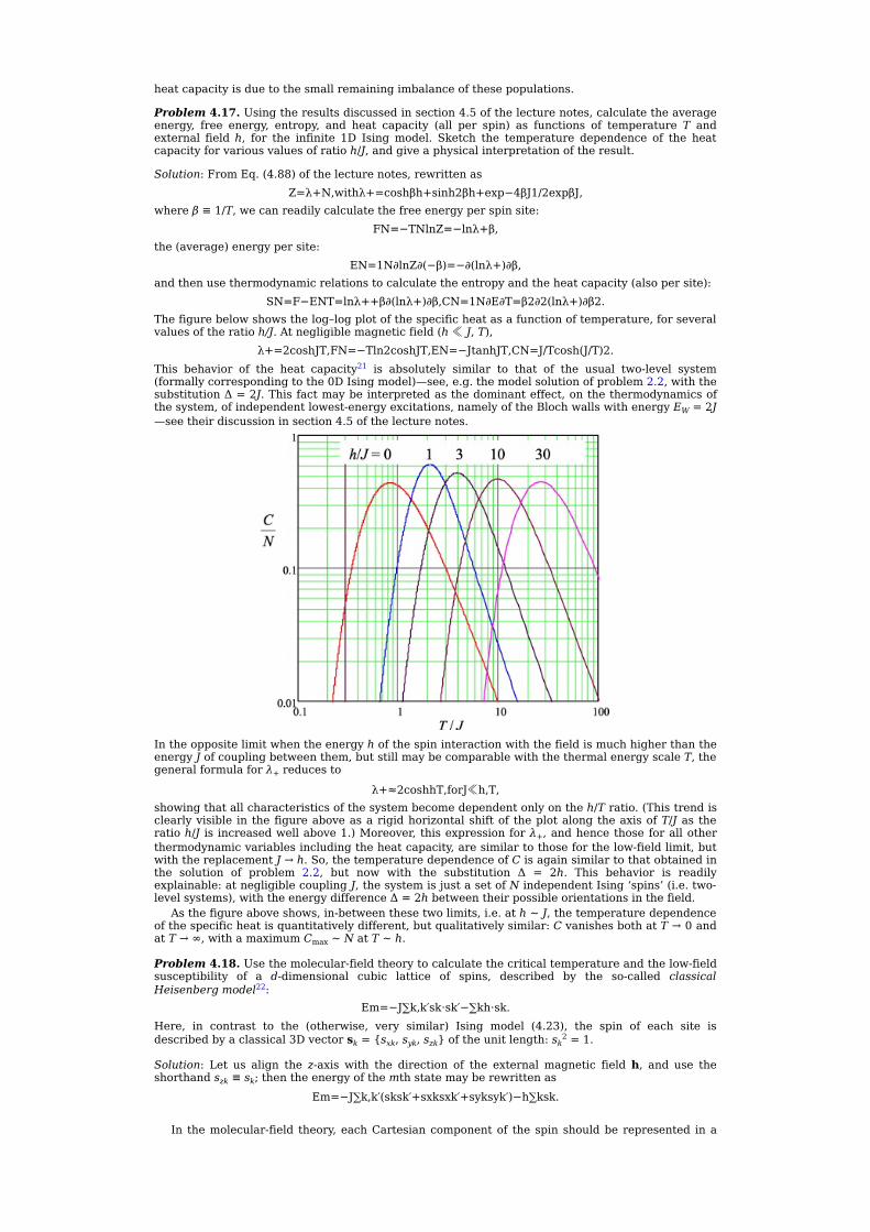
heatcapacityisduetothesmallremainingimbalanceofthesepopulations.

Problem4.17.Usingtheresultsdiscussedinsection4.5ofthelecturenotes,calculatetheaverageenergy, free energy, entropy, and heat capacity (all per spin) as functions of temperature T andexternal fieldh, for the infinite 1D Isingmodel. Sketch the temperature dependence of the heatcapacityforvariousvaluesofratioh/J,andgiveaphysicalinterpretationoftheresult.

Solution:FromEq.(4.88)ofthelecturenotes,rewrittenasZ=λ+N,withλ+=coshβh+sinh2βh+exp−4βJ1/2expβJ,

whereβ≡1/T,wecanreadilycalculatethefreeenergyperspinsite:FN=−TNlnZ=−lnλ+β,

the(average)energypersite:EN=1N∂lnZ∂(−β)=−∂(lnλ+)∂β,

andthenusethermodynamicrelationstocalculatetheentropyandtheheatcapacity(alsopersite):SN=F−ENT=lnλ++β∂(lnλ+)∂β,CN=1N∂E∂T=β2∂2(lnλ+)∂β2.

Thefigurebelowshowsthelog–logplotofthespecificheatasafunctionoftemperature,forseveralvaluesoftheratioh/J.Atnegligiblemagneticfield(h≪J,T),

λ+=2coshJT,FN=−Tln2coshJT,EN=−JtanhJT,CN=J/Tcosh(J/T)2.This behavior of the heat capacity21 is absolutely similar to that of the usual two-level system(formallycorrespondingtothe0DIsingmodel)—see,e.g.themodelsolutionofproblem2.2,withthesubstitutionΔ=2J.Thisfactmaybeinterpretedasthedominanteffect,onthethermodynamicsofthesystem,ofindependentlowest-energyexcitations,namelyoftheBlochwallswithenergyEW=2J—seetheirdiscussioninsection4.5ofthelecturenotes.

IntheoppositelimitwhentheenergyhofthespininteractionwiththefieldismuchhigherthantheenergyJofcouplingbetweenthem,butstillmaybecomparablewiththethermalenergyscaleT,thegeneralformulaforλ+reducesto

λ+≈2coshhT,forJ≪h,T,showingthatallcharacteristicsofthesystembecomedependentonlyontheh/Tratio.(ThistrendisclearlyvisibleinthefigureaboveasarigidhorizontalshiftoftheplotalongtheaxisofT/Jastheratioh/Jisincreasedwellabove1.)Moreover,thisexpressionforλ+,andhencethoseforallotherthermodynamicvariablesincludingtheheatcapacity,aresimilartothoseforthelow-fieldlimit,butwiththereplacementJ→h.So,thetemperaturedependenceofCisagainsimilartothatobtainedinthe solution of problem 2.2, but now with the substitution Δ = 2h. This behavior is readilyexplainable:atnegligiblecouplingJ,thesystemisjustasetofNindependentIsing‘spins’(i.e.two-levelsystems),withtheenergydifferenceΔ=2hbetweentheirpossibleorientationsinthefield.

Asthefigureaboveshows,in-betweenthesetwolimits,i.e.ath∼J,thetemperaturedependenceofthespecificheatisquantitativelydifferent,butqualitativelysimilar:CvanishesbothatT→0andatT→∞,withamaximumCmax∼NatT∼h.

Problem4.18.Usethemolecular-fieldtheorytocalculatethecriticaltemperatureandthelow-fieldsusceptibility of a d-dimensional cubic lattice of spins, described by the so-called classicalHeisenbergmodel22:

Em=−J∑k,k′sk⋅sk′−∑kh⋅sk.Here, in contrast to the (otherwise, very similar) Ising model (4.23), the spin of each site isdescribedbyaclassical3Dvectorsk={sxk,syk,szk}oftheunitlength:sk2=1.

Solution: Let us align the z-axis with the direction of the externalmagnetic fieldh, and use theshorthandszk≡sk;thentheenergyofthemthstatemayberewrittenas

Em=−J∑k,k′(sksk′+sxksxk′+syksyk′)−h∑ksk.

In themolecular-field theory,eachCartesiancomponentof thespinshouldberepresented ina

(*)

(**)

formsimilartoEq.(4.62)ofthelecturenotes.However,duetothesymmetryoftheproblemwithrespecttoreflectionsx→−xandy→−y,theaverage⟨s⟩≡ηmaybedifferentfromzeroonlyforthez-component.Hence the two last terms in theparentheses includeonly thesquaresof fluctuationterms:

Em=−J∑k,k′(η+s˜k)(η+s˜k′)−J∑k,k′(s˜xks˜xk′+s˜yks˜yk′)−h∑ksk,with∣s˜∣≪1.Multiplying the parentheses under the first sum, and neglecting all the terms quadratic in smallfluctuations,(seethediscussionoftransferfromEq.(4.63)toEq.(4.64)ofthelecturenotes),wegetanexpressionformallysimilartoEq.(4.64)fortheIsingmodel,

Em≈NJdη2−hef∑ksk,describing a set of N independent classical ‘spins’ sk placed into the effective (external +‘molecular’)field(4.65):

hef≡h+2Jdη.However,incontrastwiththeIsingmodel,nowskmaytakeanyvaluesfrom−1to+1.

Thissituationwasoneofthesubjectsofproblem2.4,andwecanuseitssolution.Inourcurrentnotation,itsresultfortheorderparameterreads

η≡s=cothhefT−Thef.Thisfunctionisqualitatively,butnotquantitativelysimilartoEq.(4.69),η=tanh(hef/T),fortheIsingmodel;mostimportantly,ithasathree-foldlowerslopeattheorigin:

∂η∂hef∣hef=0=13T.Thisdifference immediatelymapsonthephasetransitiontemperatureTc. Indeed,combiningEqs.(*)and(**),andlinearizingtheresultinsmallh,hef,andη(exactlyaswasdoneinsection4.4ofthelecturenotesfortheIsingmodel),forthelow-fieldsusceptibilitywegetthesameCurie–Weisslaw(4.76),

χ≡∂η∂h∣h=0=1T−Tc,butwithathreetimeslowercriticaltemperature:

Tc=2Jd3.

Thisreductionisanaturalresultofthespin-to-fieldinteractionweakeningduetotheavailabilityofintermediatevalues,−1<sk<+1,forthefield-alignedspincomponents.Inturn,thisavailabilityistheimmediateresultoftakingintoaccounttwootherCartesiancomponentsofthevectorsintheHeisenbergmodel.

1Again,itisamazinghowwellisthisexponentiallawhiddeninsidethevanderWaalsequationofstate!2Thisequationofstate,suggestedin1949,describesmostrealgasesbetterthannotonlytheoriginalvanderWaalsmodel,butalsoothertwo-parameteralternatives,suchastheBerthelot,modified-Berthelot,andDietericimodels,thoughsomeapproximationswithmorefittingparameters(suchastheSoave–Redlich–Kwongmodel)workevenbetter.3Actually,using thebulky(‘quasi-anaytical’)Tartaglia–Cardanoformulas, it ispossible toshowthat thisvalue is just (2⅔+2⅓+1).However, forparameter-freeequations,thedemonstratedmethodofnumericalsolutionisfaster,moregeneral,andperfectlysuitableformostapplications.4ThismodeliscurrentlylesspopularthantheRedlich−Kwongmodel(alsowithtwofittingparameters),whoseanalysiswasthetaskofthepreviousproblem.5Thisisofcourseveryfortunate:ificewasmoredensethanwater,thenmostlakes,rivers,andevenseaswouldfreezetothebottominwinters,andlifeontheEarthmightbepossibleonlyinthetropics.6Since,accordingtothatformula,Tc

3/2∝1/V,thefunctionP0(T)givenbythefirstofEqs.(**)actuallydoesnotdependofV—asatshouldbe—seethefigureabove.7Thistaskisessentiallythefirststepofthevariationalmethodofquantummechanics—see,e.g.PartQMsection2.9.8See,e.g.Eqs.(A.36b)and(A.36c).9See,e.g.PartQMsection3.6.10See,e.g.PartQMsection2.9.11Adiscussionoftheseparameters,aswellasofthedifferencebetweenthetype-Iandtype-IIsuperconductivity,maybefoundinPartEMsections6.4–6.5.However,thosedetailsarenotneededforthesolutionofthisproblem.12See,e.g.PartEMEq.(5.117).13Noteadifferentdescriptionoftheelectrodynamicsofsuperconductors,inwhichthesurfacesupercurrentsaredescribedexplicitly—see,e.g.PartEM section6.4.However,forbulk,type-Isuperconductorsthisalternative(andmuchmoreinvolved)analysisyieldsthesamefinalresultfor .14Ifyouneedareminder,youmayhavealookatPartEMEq.(5.108)anditsdiscussion.15NotethataccordingtoEq.(4.14)ofthelecturenotes,thefactorafterTalsogivesthedifferenceofentropiesinthesuperconductingstateandthenormalstate.16Noteagainthat(aswasdiscussedinsection1.4ofthelecturenotes),thisrelationisonlytrueiftheeffectofthefield isnotincludedintheenergyofeachparticleofthemedium,asisdone,forexample,intheIsing-typeproblems—see,e.g.thelasttermsinEqs.(4.21)and(4.23).InthelattercasethereisnodifferencebetweenthethermodynamicpotentialsGandF—unlesstheusualpressureP(oranyothergeneralizedforcebut )interferes.17Iamsurethereaderknowsthisformula—butifnot,pleaseseePartEMsection5.3and6.2,inparticularEq.(5.57).18NotethatforanopenIsingchain,thelowestexcitationhasthetwicelowerenergy—seefigure4.11anditsdiscussioninsection4.5.However,thisdifferencedoesnotaffectthevalidityofEq.(**).19See,e.g.Eq.(4.68)ofthelecturenotes,fortheparticularcasehef=h.20Aswasrepeatedlydiscussedinthiscourse,analternativewaytocalculateE,whichdoesnotrequirethepreliminarycalculationofthestates’probabilities,istouseEq.(2.61b)ofthelecturenotes:E=−∂(lnZ)/∂β.21TheformulasforF/NandE/Nare functionallydifferent fromthose in thesolutionofproblem2.2onlybecauseof theshiftof their reference levelby−J. (Thistemperature-independentshiftdoesnotaffecttheheatcapacityC≡∂E/∂T.)22Thisclassicalmodelisformallysimilartothegeneralizationofthegenuine(quantum)Heisenbergmodel(21)toarbitraryspins,andservesasitsinfinite-spinlimit.

IOPPublishing

StatisticalMechanicsProblemswithsolutionsKonstantinKLikharev

Chapter5

Fluctuations

Problem 5.1. Treating the first 30 digits of number π = 3.1415… as a statistical ensemble ofintegersk(equalto3,1,4,1,5,…),calculatetheaverage⟨k⟩,andthermsfluctuationδk.Comparethe results with those for the ensemble of completely random decimal integers 0, 1, 2,…,9, andcomment.

Solution:Thehigh-precisionvalueofπmaybeeither foundonmanyWeb sites, e.g. inWikipedia(http://en.wikipedia.org/wiki/Pi),orgeneratedbyanycalculator(say,thatonyoursmartphone)—forexample,as4·tan−1(1).Forourpurposes,weneedjustM=30firstdigits:

π=3.14159265358979323846264338327…Fromhere, the calculation can be done eitherwith a computer, bywriting and running a simplescript, using the number rounding routine readily available in virtually all numerical libraries toreformatthenumberintotheintegerarraykm=3,1,4,…,orjustbybruteforce,usingacalculator.For30digits,therequiredtimeiscomparable(andinsignificant:-).

Theresultsare:k≡1M∑m=1Mkm≈4.70;

⟨k˜2⟩≡1M∑m=1Mk˜m2≡1M∑m=1Mkm−k2=1M∑m=1Mkm2−k2≈6.08,sothat

δk≡⟨k˜2⟩1/2≈2.47.

Foraninfinitesetofrandomdecimalintegers(withequalprobabilitiesWn=1/NtotakeanyofN=10possiblevalueskn=n′≡n−1=0,1,2,…9),theexpectationvalueofknis1

k=∑n=1NknWn=1N∑n=1Nkn=1N∑n′=0N−1n′=1N(N−1)N2≡N−12=4.5.Usingthisresult,weget2

⟨k˜2⟩=1N∑n=1Nkn2−k2=1N∑k=0N−1k2−k2=1NN−1N2N−16−N−122≡N2−112=8.25,sothat

δk≡⟨k˜2⟩1/2=12N2−131/2≈2.87,i.e.virtuallythesameresultsasforthedigitsofnumberπ.

A good sanity check here is that the difference between the calculated averages of these two(verysimilar)statisticalensemblesismuchsmallerthantheirrmsuncertainties.Itisalsoimportantto understand that the relative statistical uncertainty of the random integer set would benonvanishing,andsubstantial,eveniftheirnumber(N)wasinfinite:

δkk=N+13N−11/2→N→∞=13≈0.577.

Problem 5.2. Calculate the variance of fluctuations of a magnetic moment placed into anexternalmagneticfield ,withinthesametwomodelsasinproblem2.4:3

(i)aspin-½withagyromagneticratioγ,and(ii)aclassicalmagneticmoment ,ofafixedmagnitude ,butwithfreeorientation,

bothinthermalequilibriumattemperatureT.Discussandcomparetheresults.

Hint:MindallthreeCartesiancomponentsofthevector .

Solutions:

(i)Aswasdiscussedinthemodelsolutionofproblems2.2–2.4,inthiscasethestationaryvaluesofthe magnetic moment are , where and nz is the field’s direction, and thecorrespondingeigenenergiesare

sothattheirprobabilitiesW±inthecanonicalensembleare

W±=1Zexp∓hT=exp∓h/Texp+h/T+exp−h/T,withW++W−=1,andtheaveragemagneticmomentisdirectedalongthefield: ,with

Theaveragesquareof maybecalculatedsimilarly:

NowwecanusethegeneralEq.(5.4b)of the lecturenotes tocalculate thevarianceofmoment’sfluctuations:

Note that this resultmay be also obtained in a differentway, usingEq. (5.37a) of the lecture

notes, and the analogy between two canonical pairs of variables: {−P, V} for a system undermechanicalpressure,and forasinglemagneticmoment—orratheritscomponentinthedirectionofthefield4.ThisanalogyimmediatelyyieldsEq.(*)again:

Inthelimitofrelativelyhightemperatures,i.e.relativelylowfields(h≪T),thedenominatorof

thisexpressiontends to1,so that themoment’svariance is largest,approaching ,while in theopposite,low-temperature(high-field)limit,thefluctuationsareexponentiallysmall:

ThisisanaturalresultforasystemwiththeenergygapΔ=2h,separatingthegroundstateofthesystemfromits(only)excitedstate.

Now let us consider two other components of themagneticmoment. Their averages evidentlyequalzeroduetotheaxialsymmetryofthesystem:

andthesamesymmetrymaybeusedtowrite ,sothatsince ,

Here we should avoid the error of taking equal to . Indeed, in quantum mechanics theexpectationvalueof the spin’s square is ⟨S2⟩=ℏ2s(s+1), so that for spin-½,with s=½, ⟨S2⟩=(3/4)ℏ2. (Since this isequality isvalid foranyquantumstateof thesystem, it isalsovalid for theaverageoveranystatisticalensembleaswell,includingthatinthermodynamicequilibrium.)Hence,for ,wehave

sothat

—thesameresultasfor intheabsenceofthefield.So, the fluctuations of the lateral components of the magnetic moment are temperature-

independent,andphysicallyarecausedjustbytheirquantumuncertainty.(WemaysaythatevenatT=0thesefluctuationsareultimatelylarge,sothatthermalexcitationsofthespinatT>0cannotincreasethem.)

(ii)Aswasdiscussedinthemodelsolutionofproblem2.4,inthismodeltheprobabilitydistributioniscontinuous,withtheangulardensity

(withthesamenotation, ,forthenormalizedfield),givingthefollowingaverages:

Wemaynowcalculate theaveragesquaresofallCartesiancomponentsof thevector inthe

sameway.However, due to the axial symmetry of theproblem, those of thex- andy-componentshavetobeequal,sothatitisconvenienttocalculatethembothinoneshot:

Theseintegralsmaybeworkedoutexactlyasinthesolutionofproblem2.4,byintroducingthenewvariableξ≡ (h/T)cosθ, so that cosθ= (T/h)ξ, sinθdθ≡−d(cosθ)=−(T/h)dξ, and sin2θ=1−(T/h)2ξ2:

∫0πexphcosθTsinθdθ=−Th∫−h/T+h/Teξdξ=−Th[eξ]−h/T+h/T=−2ThsinhhT,∫0πsin2θexphcosθTsinθdθ=−Th∫−h/T+h/T1−Th2ξ2eξdξ≡−Th∫−h/T+h/Teξdξ+Th3∫

−h/T+h/Tξ2eξdξ.The firstof these two integrals isexactly thesameaswas (easily :-)workedoutabove,while thesecondonerequirestwosequentialintegrationsbyparts,giving

∫−h/T+h/Tξ2eξdξ=(ξ2−2ξ+2)eξ−h/T+h/T=2hT2+2sinhhT−4hTcoshhT.Asaresult,weget

Finally,sincethemagnitude ofthevector isthesameinallitspossiblestates,wemaywrite

so that the calculation of the square of the remaining, field-aligned component of the magneticmomentmaybeperformedverysimply:

andthegeneralrelation(5.4b)yields

Aswasalreadydiscussedinthemodelsolutionofproblem2.4,inthehigh-temperature(low-field)

limith≪T,theexpressionintheparenthesesparticipatinginEqs.(**)and(***)approachesh/3T≪1,sothatourresultsarereducedtoaverysimple,field-independentexpression

Thisisverynatural,becauseintheabsenceofthefield,thesystemisfullyisotropic.However, in the opposite, low-temperature (high-field) limit, when the same expression in the

parenthesestendsto1−T/h,Eqs.(**)and(***)giveverydifferentresultsforthefield-alignedandfield-normalcomponents:

Thephysicalreasonforthisdifferenceisthatsmalldeviationsofthemomentvectorfromthefield-aligneddirectionnzgiveacontributiontotheenergy,whichisquadraticin and :

sothattheirvarianceshaveto(anddo!)satisfytheequipartitiontheorem(2.48):

On the other hand, the deviations of the z-component of the momentum from its valuecorrespondingtotheexactalignment,inthislimitaremuchsmaller:

asaresult,theirvarianceisofahigherorderinthesmallparameterT/h.Nowcomparingtheresultsforthetwomodelsofaspininmagneticfield,weseethattheyare

rather different. Most significantly, in the low-temperature limit, the classical Heisenberg model(which isasymptoticallycorrect for largevaluesofspin,s≫1)doesnotexhibit theexponentiallysmallfluctuationsof ,whichare typical fors=½ (andany finitevalueof spin),becauseof the

(*)

availabilityofintermediatestateswith0<θ<π,fillingthegapbetweentwoextremevalues(E=±h)oftheenergy.

Problem 5.3. For a field-free, two-site Ising systemwith energy valuesEm = −Js1s2, in thermalequilibrium at temperature T, calculate the variance of energy fluctuations. Explore the low-temperatureandhigh-temperaturelimitsoftheresult.

Solution:Thissystemhastwodoubly-degeneratevaluesofitsenergyE:Em=−J,fors1=s2,+J,fors1=−s2.

HenceitsstatisticalsumisZ=2expJT+2exp−JT≡4coshJT,

theaverageofthesystem’senergyisE=1Z∑mEmexp−EmT=14cosh(J/T)2Jexp−JT−2JexpJT≡−JtanhJT,

andthatofE2is⟨E2⟩=1Z∑mEm2exp−EmT=14cosh(J/T)2J2exp−JT+2J2expJT≡J2,

sothattheenergyfluctuationvariance⟨E˜2⟩=⟨E2⟩−E2=J21−tanh2JT≡J2cosh2(J/T).

Alternatively,thesameresultmaybeobtainedusingEq.(5.19)ofthelecturenotes,as∂⟨E⟩/∂(−β).At low temperatures, T≪ J, the function cosh(J/T) is very large, so that the fluctuations are

exponentiallysmall,duetothegap2Jintheenergyspectrumofthesystem.Ontheotherhand,inthe opposite limit of high temperatures, cosh(J/T) → 1, and the variance approaches thetemperature-independentvalueJ2.

Problem 5.4. For a uniform three-site Ising ring with ferromagnetic coupling (and no externalfield),calculatethecorrelationcoefficientsKs≡⟨sksk′⟩forbothk=k′andk≠k′.

Solution:InallIsingmodels,each‘spin’skmaytakeonlythevalues±1,sothatitssquareequals1in any state of the system, and hence ⟨sk2⟩ equals 1 for any parameters. However, the mutualcorrelationcoefficients⟨sksk′⟩,5withk′≠k,requirecalculation.

Aswasalreadydiscussed in themodelsolutionofproblem4.15, theenergyofaring’sstate isgivenbyEq.(4.78)ofthelecturenotes(withN=3andh=0):

Em=−J(s1s2+s2s3+s3s1),withJ>0.Thesystemevidentlyhas23=8differentstates.Intwoofthemthe‘spins’areallaligned(ineitheroftwopossibledirections),sothatforeachofthemEm=−3J.Inallremainingsixstates,onespinhas a direction different from its two counterparts, so thatEm = −J(+1 − 1 − 1) = +J. Hence,system’sstatisticalsumis

Z=2exp3JT+6exp−JT.sothattheprobabilitiesofhavingsome(notparticular)statesofthesetwokindsareequalto

W1=2exp3J/T2exp3J/T+6exp−J/T,W2=6exp−J/T2exp3J/T+6exp−J/T,withW1+W2=1.

Sincetheproductsksk′(withk≠k′)maytakeonlytwovalues:(+1)whenthespinskandk′arealignedwitheachother,and(−1)otherwise,wemaywrite

Ks≡⟨sksk′⟩=(+1)W++(−1)W−=W+−W−,whereW±arethecorrespondingprobabilities,withW++W−=1.Ifthespinsareallaligned(State1 in the abovenomenclature), thenall sksk′=1.However, if one of them ismisaligned (State2),thereisonly1/3chancethatanygivenpairofspinskandk′isaligned(becausethisisthechancethatthespinnumberk″≠k,k′,notinvolvedinthispair,ismisaligned).Hence,W+=W1+(1/3)W2,whileW−=1−W+=(2/3)W2,andfinally:

Ks=W+−W−=W1+13W2−23W2=1−exp−4J/T1+3exp−4J/T,foranyk′≠k.

This result shows that in the low temperature limit, T≪ J, themutual correlation coefficientapproaches1.This isnatural,becausetheprobabilityW1of the fullspinalignmentapproaches1,whileW2 isexponentiallysmall. Intheopposite limitofhightemperatures,exp{−4JT}≈1−4JT,andthemutualcorrelationislow:

Ks≈JT≪1,fork′≠k.Note, however, that ⟨sksk′⟩ is positive for any ratio J/T. This is natural, because the ferromagneticcoupling,withJ>0,alwaysfavorsspinalignment.

Problem 5.5.* For a field-free 1D Ising system of N ≫ 1 ‘spins’, in thermal equilibrium attemperatureT,calculatethecorrelationcoefficientKs≡⟨slsl+n⟩,whereland(l+n)arethenumbersoftwospecificspinsinthechain.

Hint:Youmayliketostartwiththecalculationofthestatisticalsumforanopen-endedchainwitharbitraryN>1andarbitrarycouplingcoefficientsJk,andthenconsideritsmixedpartialderivativeoverapartoftheseparameters.

Solution:Foranopen-endedchainoutsideofexternal field(h=0),witharbitraryJk,Eq. (4.23)ofthelecturenotesmayberewrittenas

Em=−∑k=1N−1Jksksk+1.Thestatisticalsumofsuchachainis

ZN=∑mexp−EmT=∑sk=±1,fork=1,2,…,Nexp∑k=1N−1JkTsksk+1≡∑sk=±1,fork=1,2,…,N∏k=1N

(**)

(***)

(****)

−1expJkTsksk+1.Letusassumethatwealreadyknowthissum(of2N terms),anduse it tocalculate thestatisticalsumZN+1(of2N+1terms)forasimilarchainofZN+1spins.TheenergyofthenewsystemdiffersfromthatoftheoldoneonlybytheadditionoftheenergyΔ=−JNsNsN+1ofthenewcouplinglink.Foranyfixedsetof‘old’spins{s1,s2,…,sN},theadditionalenergymaytakeonlytwovalues,±JN,thusreplacingeachtermofthesum(*)withtwoterms,withadditionalfactorsexp{−Δ/T}=exp{±JN/T}.Asaresult,weget

ZN+1=∑sk=±1,fork=1,2,…,N+1exp∑k=1N−1JkTsksk+1exp−JNT+exp+JNT≡ZN×2coshJNT.

Nowwemayapplythissimplerecurrencerelationsequentially,startingfromtheeasyparticularcaseN=2,i.e.forthesystemwithjustonelink,whosestatisticalsumhasonlyfourterms,withtwoequalpairs:

Z2=∑sk=±1,fork=1,2expJ1Ts1s2=2exp+J1T+2exp−J1T≡4coshJ1T.TheresultforanarbitraryN⩾2is

ZN=4coshJ1T×2coshJ2T×…×2coshJN−1T≡2∏k=1N−12coshJkT.

Notethatforauniformchain,withJ1=J2=…=JN−1≡J,thisexpressionbecomesZN=22coshJTN−1,

whichisdifferentfromthatgivenbyEq.(4.88)ofthelecturenotes,foraringof(N−1)sites,forourcurrentcaseh=0,onlybytheinconsequentialfactorof2.

NowwearereadytocalculatethecoefficientsKs≡⟨slsl+n⟩,which(forn≠0)describethemutualcorrelationofvaluesoftwospinsatthedistancenfromeachother.Foranopen-endchainoflengthN,againwitharbitrarycoefficientsJk,thegeneralEq.(2.7),withtheGibbs-distributionprobabilitiesWm=exp{−Em/T}/ZN,gives

Ks=1ZN∑sk=±1,fork=1,2,…,Nslsl+nexp∑k=1N−1JkTsksk+1≡1ZN∑sk=±1,fork=1,2,…,Nslsl+n∏k=1N−1expJkTsksk+1,

whereZN isgivenbyEq.(**).Letususethefactthatallsk2=1torewritethisexpression inthemathematically-equivalentform

Ks=1ZN∑sk=±1,fork=1,2,…,N(slsl+1)(sl+1sl+2)…(sl+n−1sl+n)∏k=1N−1expJkTsksk+1,andcompareitwiththefollowingpartialderivative:

Dn≡∂nZN∂Jl∂Jl+1…∂Jl+n−1.Ononehand,ifwedifferentiateZNinthelastformofEq.(*),andthenuseEq.(***)forKs,weget

Dn≡∑sk=±1,fork=1,2,…,N∂n∂Jl∂Jl+1…∂Jl+n−1∏k=1N−1expJkTsksk+1=1Tn∑sk=±1,fork=1,2,…,N(slsl+1)(sl+1sl+2)…(sl+n−1sl+n)∏k=1N−1expJkTsksk+1≡1TnKsZN.

Ontheotherhand,ifweuseZNintheformEq.(**),thesamederivativegives

Dn≡∂n∂Jl∂Jl+1…∂Jl+n−12∏k=1N−12coshJkT=2∏k=1l−12coshJkT∏k=ll+n−11T2sinhJkT∏k=l+nN−12coshJkT.

Comparingthesetwoexpressions forDn,withZNagain taken fromEq. (**),wegetasurprisinglysimpleresult:

Ks=∏k=ll+n−1sinhJkT/∏k=ll+n−1coshJkT≡∏k=ll+n−1tanhJkT,valid for arbitrary coupling coefficients Jk (both inside and outside of the interval [l, l + n]) andarbitrarypositionsofthesitesland(l+n)intheopenchain6.

Foraparticularcaseofauniformchain,theresultbecomesevensimpler,anddependsonlyonthedistancenbetweentheinvolvedsites:

Ks=Ksn=tanhnJT≡exp−nnc,wherethe(notnecessarilyinteger)constantnc,

nc≡−1lntanhJ/T→1/lnT/J≪1,atJ≪T,exp2J/T/2≫1,atJ≫T,playstheroleofthecorrelationradiusofthis1Dsystem—cf.Eq.(4.30)ofthelecturenotes(whosepre-exponentialfactor,aswellasEq.(4.31),arevalidonlyforsystemswithnonvanishingTc).

Problem5.6.WithintheframeworkofWeiss’molecular-fieldtheory,calculatethevarianceofspinfluctuationsinthed-dimensionalIsingmodel.Usetheresulttoderivetheconditionsofquantitativevalidityofthistheory.

Solution: Since in the Ising model, the variable sk2 = (±1)2 ≡ 1 in any state of the system, itsstatistical average also equals 1 within any (reasonable:-) solution of the model—including theWeiss’approximation.CombiningthisresultwithEq.(4.69)ofthelecturenotes,weget

s˜k2=sk2−⟨sk⟩2=sk2−η2=1−tanh2(hef/T)≡1cosh2(hef/T).(Actually, we could get this result from Eq. (*) of the model solution of problem 5.2, with thereplacementh→hef,whichistheessenceoftheWeiss’approach.)

ThekeyassumptionofWeiss’theoryis⟨s˜k2⟩≪η2.Reviewingthedependenceofhef≡h+2Jdηonparametersofthesystem,discussedinsection4.4(see,inparticular,figures4.8and4.9),wemayconcludethatforstablestationarystates,thisstronginequalityisfulfilled(andhencethetheoryisasymptoticallycorrect)at:

(i)lowtemperatures,T≪2Jd(meaning,withinthattheory,thatT≪Tc),atanyfieldh,and

(ii)highexternalfields,h2≫T2,atanyratio2Jd/T.

(*)

(**)

(***)

(*)

(**)

(***)

(****)

Problem5.7.Calculatethevarianceoffluctuationsoftheenergyofaquantumharmonicoscillatorwithfrequencyω,inthermalequilibriumattemperatureT,andexpressitviatheaveragevalueoftheenergy.

Solution:PluggingtheresultgivenbyEq.(2.72)ofthelecturenotesfortheaverageenergyEoftheoscillator,intheform

E=ℏωeβℏω−1,whereβ≡1/T,intothegeneralEq.(5.19),weget

⟨E˜2⟩=−∂E∂β=−∂∂βℏωeβℏω−1=ℏωeβℏω−12eβℏω≡ℏωeℏω/T−12eℏω/T.

ItisstraightforwardtoverifythatEqs.(*)and(**)aresimplyrelated:⟨E˜2⟩=ℏωE+E2.

Thismeans,inparticular,thatthermsfluctuationofenergyisalwayslargerthanitsaveragevalue:δE⩾E.

Note,however,thatthisrelation,aswellasEq.(***)assuch7,arevalidonlyifEisreferredtothe

ground-stateenergyℏω/2oftheoscillator(asitisinEq.(2.72)ofthelecturenotes);itisinvalidforthetotalenergy,givenbyEq.(2.80),whichisreferredtothepotentialenergy’szero:

Etotal≡E+ℏω2.Forthisreferencepoint,Eq.(***)takesadifferentform:

⟨E˜2⟩=⟨Etotal⟩2−ℏω22,sothattherelationbetweenthermsfluctuationofenergyanditsaverageisopposite:

δE⩽⟨Etotal⟩.

Problem5.8.ThespontaneouselectromagneticfieldinaclosedvolumeVisinthermalequilibriumwithtemperatureT.Assuming thatV issufficiently large,calculate thevarianceof fluctuationsofthe totalenergyof the field,andexpress the resultvia itsaverageenergyand temperature.HowlargeshouldthevolumeVbeforyourresultstobequalitativelyvalid?Evaluatethis limitationforroomtemperature.

Solution:Aswasdiscussed in section2.6(i)of the lecturenotes, thespontaneouselectromagneticfield in a sufficiently large closed volume V may be represented as a sum of independent fieldoscillatorswiththespectraldensity(2.83):

dN=Vω2π2c3dω.InthethermalequilibriumattemperatureT, theaverageenergyofsuchanoscillator (referredtotheground-stateenergyℏω/2)isgivenbyEq.(2.72),

E=ℏωeℏω/T−1,whilethecalculationofthevarianceof its fluctuationswasthetaskofthepreviousproblem,withthefollowingresult:

⟨E˜2⟩=ℏωeℏω/T−12eℏω/T.

Since the fluctuations of oscillators with different frequencies (and with different fieldpolarizations at the same frequency) are independent, and the fluctuations of their energies areuncorrelated,thevarianceofthetotalenergyEΣmaybeobtainedbythesummationofthepartialvariances:

E˜Σ2=∫ω=0ω=∞⟨E˜2⟩dN.BysubstitutionofEqs.(*)and(***),thisintegralmaybereducedtoatableintegral—butnotaverypleasingone.However,wemayre-usethesimplerintegralalreadyworkedoutinsection2.6forthecalculationoftheaveragetotalenergyoftheradiation—seeEq.(2.88):

⟨EΣ⟩=∫ω=0ω=∞EdN=∫0∞ℏωeℏω/T−1Vω2π2c3dω=π215VT4ℏ3c3≡π215Vℏ3c3β−4.Forthat,letususethegeneralEq.(5.19)towrite

E˜Σ2=−∫ω=0ω=∞∂E∂βdN≡−∫0∞∂E∂βdNdωdω.Since thedensityof statesdN/dω is temperature-independent,wemay take thepartialderivativeoperator ∂/∂β from under the integration sign, and notice that the remaining integral is just theaveragetotalenergy(****),sothat

E˜Σ2=−∂∂β∫ω=0ω=∞EdN≡−∂∂β⟨EΣ⟩=π215Vℏ3c34β−5≡4T×π215VT4ℏ3c3.NowusingEq.(****)again,wemayreducetheresulttoaverysimpleform:

E˜Σ2=4T⟨EΣ⟩,whichshowsthattherelativermsfluctuationofthetotalenergy,

δEΣ⟨EΣ⟩≡E˜Σ21/2⟨EΣ⟩=2T⟨EΣ⟩1/2∝1T3/2V1/2,decreaseswiththegrowthofbothtemperatureandvolume.(Thisresulthasimportantimplicationsfor accurate measurements of the fundamental anisotropy of the cosmic microwave backgroundradiation.)

Proceedingtothesecondquestionoftheassignment,notethatEq.(*)isstrictlyvalidonlyifdN≫ 1, i.e. if the volumeV ismuch larger that than the cube of thewavelength:V≫c3/ω3 for allsubstantial frequencies. As was discussed in section 2.6(i), in thermal equilibrium, their scale isgivenbytherelation(2.87):ℏωmax∼T,sothattherequiredconditionis

V≫cωmax3∼ℏcT3.Forroomtemperature(T≡kBTK≈1.38×10−23JK−1×300K≈4×10−21J),theright-handsideof

(*)

(**)

(***)

(****)

thisrelationisoftheorderof10−15m3≡(10μm)3, i.e. issmallonthehumanscale,butnotquitemicroscopic.

Problem5.9.ExpressthermsuncertaintyoftheoccupancyNkofacertainenergylevelεkby:

(i)aclassicalparticle,(ii)afermion,and(iii)aboson,

inthermodynamicequilibrium,viaitsaverageoccupancy⟨Nk⟩,andcomparetheresults.

Solutions: Aswas discussed in section 2.8 of the lecture notes, for a statistical ensemble of non-interactingparticleswemayusethegrandcanonicaldistributionforthesub-ensembleofparticleson the sameenergy level.HencewemayapplyEq. (5.24) of the lecturenotes, derived from thisdistribution,totheleveloccupancyNk:

N˜k2=T∂⟨Nk⟩∂μ.(i)Foraclassicalparticle,thedependenceof⟨Nk⟩onthechemicalpotentialμisgivenbythesameformula(5.25)asforthetotalnumberofparticles,

⟨Nk⟩∝expμT,sothatwemayrepeatthe(verysimple)derivationofEq.(5.27)togetthesimilarresult:

N˜k2=⟨Nk⟩,i.e.δNk=⟨Nk⟩1/2.(ii)–(iii)Forfermionsandbosons,⟨Nk⟩isgivenbyverysimilarexpressions(2.115)and(2.118),whichmaybemergedintoasingleformula(justaswasdoneinsection3.2):

⟨Nk⟩=1exp(εk−μ)/T±1,withtheuppersignforfermionsandthelowersignforbosons.NowapplyingEq.(*)tothisformula,weget

N˜k2=exp(εk−μ)/Texp(εk−μ)/T±12.Expressingtheexponent,participatinginbothpartsofthisfraction,fromEq.(***),

exp(εk−μ)/T=1⟨Nk⟩∓1,andpluggingthisexpressionintoEq.(****),wegetthefinalresult

N˜k2=⟨Nk⟩1∓⟨Nk⟩,i.e.δNk=⟨Nk⟩1∓⟨Nk⟩1/2.

ComparingitwithEq.(**)weseethat,foragivenaveragevalue⟨Nk⟩oftheleveloccupancy,itsfluctuations in the case of fermions are smaller, and in the case of bosons, larger than those forclassicalparticles.(Alltheseexpressionstendtoeachotherat⟨Nk⟩→0,i.e. intheclassicallimit—seeEq.(3.1)ofthelecturenotes.)

Problem 5.10. Express the variance of the number of particles, ⟨N˜2⟩V,T,μ, via the isothermalcompressibility κT≡−(1/V)(∂V/∂P)T,N of the same single-phase system, in thermal equilibrium attemperatureT.

Solution:AccordingtoEq.(5.24)ofthelecturenotes,⟨N˜2⟩V,T,μ=T∂N∂μV,T.

Butashasbeenprovedinthesolutionofproblem1.10,theisothermalcompressibilityofasingle-phasesystemmaybeexpressedviathesamepartialderivative:

κT=VN2∂N∂μV,T.Comparingtheaboveexpressions,weget

⟨N˜2⟩V,T,μ=κTTN2V.

Note,however,thatEq.(5.24)hasbeenderivedforthegrandcanonicalensembleoffixed-volumesystems,sothatourresultisalsovalidforsuchanensemble,i.e.ifthechemicalpotentialμdoesnotfluctuate.(Incontrast,inacanonicalensemble,thenumberofparticlesdoesnotfluctuateatall,butμmay.)

Problem 5.11.* Starting from theMaxwell distribution of velocities, calculate the low-frequencyspectraldensityoffluctuationsofthepressureP(t)ofanidealgasofNclassicalparticles,inthermalequilibrium at temperature T, and estimate their variance. Compare the former result with thesolutionofproblem3.2.

Hint:Youmayconsideracylindrically-shapedcontainerofvolumeV=LA (see the figure above),calculatefluctuationsoftheforce exertedbytheconfinedparticlesonitsplanelidofareaA,approximating it as a delta-correlated process (5.62), and then recalculate the fluctuations intothoseofthepressure .

Solution:Foronemolecule, theconstantc in theapproximate formula for the

force it exerts on the lid in the direction normal to its plane (see the figure above),may becalculatedastheintegral,

over a time interval larger than the collision duration τc, but smaller than the time intervalbetweentwosequentialcollisions,with beingthecomponentof theparticle’svelocity

component in the direction normal to the lid. Due to particle independence, we can replace theaveraginginthisexpression,overastatisticalensembleofsimilarparticles(withthesame ),withthatoverthetimeintervalΔt:

…=1Δt∫…dt.Introducing,insteadofτ,anewindependentvariablet′≡t+τ,weget

Thetimeintegral inthelastformulais justthemomentumtransferredfromtheparticletothelidduringoneelasticcollision,equalto ,sothat

Forsuchashort-pulseprocessas (see,e.g.figure5.4ofthelecturenotes),itstimeaverage,

isnegligibleincomparisonwithitsrmsfluctuation:

(this almost evident fact will be proved a posteriori, in just a minute), so that Eq. (*) may berewrittenas

According to Eq. (5.62), this delta-correlated process has the following low-frequency spectraldensity:

(NowwemayproveEq.(**)bymakingtheestimateofthermsfluctuation,givenbyEq.(5.60):

whereωmaxisthefrequencywherethespectraldensitystartstodropfromitslow-frequencyvalue.Besidessomenumericalfactoroftheorderof1(itsexactcalculationwouldrequireaspecificmodeloftheparticlecollisionswiththelid),thisfrequencyisjustthereciprocalcollisiontime,sothatwemaycontinueas

Foragastobehaveideally,theintervalsΔtbetweenlidhitsbymoleculeshavetobemuchlongerthanthehitdurationτc,sothatthelastfactorhastobemuchlargerthan1,provingEq.(**).)

Thespectraldensitiesof independent force fluctuations fromdifferentmolecules (eachwith itsownvelocity )justaddup,sothatforthelow-frequencyspectraldensityofthenetforceweget

This statistical average may be readily calculated from the 1D Maxwell distribution, i.e. theGaussiandistributionwiththevariance :

Thisisatableintegral8,equalto1!/2=½,sothatweget

and,finally,thespectraldensityofthepressure is

Anapproximatebutfairestimateofthepressurefluctuationvariancemaynowbeachieved,as

above, by replacing the integral participating in the last form of Eq. (5.60) with the productSP(0)ωmax∼SP(0)/τc:9

(****)

(*)

This estimate differs from the ‘thermodynamic’ formula cited in a footnote in section 5.3 of thelecture notes. For an classical ideal gas, with the average pressure ⟨P⟩ = NT/V, held at fixedtemperatureT,andhencewith(−∂⟨P⟩/∂V)T=NT/V2,thatformulayields

⟨P˜2⟩=NT2V2.(WRONG!)Thedifferenceisduetothesharp-pulsenatureofthepressureforce(whichcannotbeaccountedforin the way the ‘thermodynamic’ formula is usually derived), extending the pressure fluctuationbandwidth to frequencies ∼1/τc, much higher that the value implied by the‘thermodynamic’ formula. (This fact, and the deficiency of the traditional derivation of Eq. (****),wererecognizedlongago10,butthisformulaisstillbeingcopiedfromoldtextbookstonewones.)

NowletuscompareEq.(***),rewrittenforthetotalforce exertedbyallmolecules,

withthedragcoefficientcalculatedinthesolutionofproblem3.2,η=NAV8mTπ1/2T.

Weseethattheyaresimplyrelated:

In this equality, we may readily recognize the general relation (5.73) between the thermal

fluctuations and dissipation, i.e. the classical limit of the fluctuation–dissipation theorem (5.98)—thusprovidingagoodsanitycheckofEq.(***).

Problem5.12.Calculate the low-frequencyspectraldensityof fluctuationsof theelectriccurrentI(t)duetorandompassageofchargedparticlesbetweentwoconductingelectrodes—seethefigurebelow.Assume that theparticles areemitted, at random times,byoneof theelectrodes, andarefully absorbed by the counterpart electrode. Can your result be mapped on some aspect of theelectromagneticblackbodyradiation?

Hint:ForthecurrentI(t),usethesamedelta-correlated-processapproximationasfortheforceinthepreviousproblem.

Solution:Attheseconditions,thecurrentI(t)isasumofshort,independentpulses,withadurationτc of the order of the time of particle’s passagebetween the electrodes.On the time scalemuchlargerthanτcwecanwrite.

I(t)I(t+τ)=Cδ(τ).Integrating both parts of this equation over the time of one current pulse, and transforming itexactlyasinthemodelsolutionofthepreviousproblem,weget

C=∫I(t)I(t+τ)dτ=ν∫I(t)dt2>0,whereν istheaverage(cyclic) frequencyofsinge-electronpassageevents.Butthe integral inthebrackets is just the electric chargeq of one particle. Taking into account that the product qν isevidentlyequaltothetime-averaged(‘dc’)currentI¯,weget

C=νq2=∣qI¯∣,i.e.I(t)I(t+τ)=∣qI¯∣δ(τ).(Since,unlikeinthepreviousproblem,allthepulse‘areas’∫I(t)dtareequaltoq,andhencetoeachother, their statistical averaging isunnecessary.)NowEq. (5.62) of the lecturenotes immediatelyyieldsaconstantlow-frequencyspectraldensity:

SIω=SI(0)=∣qI¯∣2π,forω≪2πν.UsingEq.(5.61),thisexpressionmayberecastintoitscommonform

⟨I˜2⟩Δν=2∣qI¯∣Δν.

ThisisthefamousSchottkyformulafortheshotnoise,whichwasbrieflymentionedinsection5.5ofthelecturenotes—seeEq.(5.82)anditsdiscussion.(Itwasfirstderivedin1918byWSchottkyusing a different approach, based on the Poisson probability distribution (5.31) of the number ofparticlespassingthroughthesystemduringatimeintervalΔt≫τc.)

Nowproceedingtotheelectromagneticradiationoffrequencyω,letsomesourceofit(say,asetofsimilaratomsbeingexternallyexcitedtoanenergylevelEe=Eg+ℏω)emititsquanta,eachwithenergyℏω,independentlyofeachother,andthebackflowofradiationbenegligible.Thenreplacingthe above arguments for the electric current I(t) with those for the power flow of theelectromagnetic radiation (time-averaged over a time interval much larger than ), we mayexpect the spectral density of its fluctuations (frequently called the photon shot noise) to beexpressedbytheformulaanalogoustoEq.(*):

(*)

Boththedetailedquantumtheoreticalanalysisofradiation,andexperiments (mostly, inoptical

photoncounting)confirmthisresult.Unfortunately,itsmoreformalderivationwouldrequiremuchmoretimethanIhaveinthisseries,sothatIhavetoreferthereadertospecialliterature11.

Problem 5.13. 12 A very long, uniform string, of mass μ per unit length, is attached to a firmsupport, and stretched with a constant force (‘tension’) —see the figure below. Calculate thespectral density of the random force exerted by the string on the support point, within theplanenormaltoitslength,inthermalequilibriumattemperatureT.

Hint:Youmayassumethatthestringissolongthatatransversewave,propagatingalongitfromthesupportpoint,nevercomesback.

Solution: Temporarily, let us ignore the fluctuations, and assume that the support point is beingslightly moved, in the plane normal to the string, following some externally-fixed law q0(t),independentofthestringmotion.(Thismotionmaybetwo-dimensional,sothatgenerallyithastobedescribedwitha2Dvector.)Suchdisplacementimposestheboundarycondition,

q0,t=q0(t),onthetransversewavesq(z,t)thatareexcited,bythismotion,topropagatealongthestring.(Herezistheaxisdirectedalongthestring,withtheoriginattheattachmentpoint.)Classicalmechanicssays13thatifsuchwavesarenottoolarge14,theirdynamicsofobeysthelinearwaveequation

AttheconditiongivenintheHint15,thesolutionofthisequation,satisfyingtheboundarycondition(*),hastheformofawave,

traveling from the wall, with the velocity . Such a wave of string displacements isaccompaniedbythefollowingwaveofthetransverseforce16:

exerted by the ‘right’ part of the string (as seen from the given point z) on its ‘left’ part. (Theconstant iscalledthewaveimpedanceofthesystem.)

Applying this result to thepointz=0,wesee that thestringprovides, for thesupportpoint’smotion,thedamping(drag)forcedescribedbyEq.(5.64)ofthelecturenotes, ,withthedragcoefficient , i.e.hasthegeneralizedsusceptibility —seeEqs.(5.89)and(5.90)ofthelecturenotes17.Sincethisresultisvalidregardlessoftheactualmotionq0(t),wemayuseittospelloutEq.(5.98)forourparticularcase:

Inhuman-scalesystems,thedivergenceofthisresultatω→∞iscutoff(atleast)bytheviolation

ofthealreadymentionedcondition∣∂q(z,t)/∂z∣≪1ofitsvalidity.Indeed,accordingtoEq.(**),thederivativeonitsleft-handsideofthisinequalityequals ,andforasinusoidaloscillationwithamplitudeAandfrequencyω,itsmagnitudegrowswithfrequencyas .

Problem5.14.18Eachoftwo3Dharmonicoscillators,withmassmandresonancefrequencyω0,hastheelectricdipolemomentd=qs,wheresistheoscillator’sdisplacementfromitsequilibriumposition.UsetheLangevinformalismtocalculatetheaveragepotentialofelectrostaticinteractionof these twooscillators (a particular case of the so-calledLondondispersion force), separatedbydistance r≫ (T/mω0

2)½, in thermal equilibrium at temperature T≫ ℏω0. Also, explain why theapproachusedinthesolutionoftheverysimilarproblem2.15isnotdirectlyapplicabletothiscase.

Hint:Youmayliketousethefollowingintegral:∫0∞1−ξ2(1−ξ2)2+αξ22dξ=π4α.

Solution:Letustemporarilyprescribetoeachoscillatorsomenonvanishingdampingparameterδ≡η/2m.Iftheinteractionbetweentheoscillatorsisnegligible,intheclassicallimiteachofthemmaybedescribedbytheLangevinequation(5.65),withκ=mω0

2,validforeachCartesiancomponentofthedisplacementvectors.Mergingtheseequationsintothevectorform,andmultiplyingalltermsbytheratioq/m,fortheelectricdipolemomentdoftheoscillatorweget

Since the Langevin forces exerted on each dipole by their dissipative environments are random,independent,andisotropic,soarethespontaneouslyinduceddipolemomentsd1,2.Asaresult,theenergyoftheirelectrostaticinteraction19,

U=14πε0r3(d1xd2x+d1yd2y−2d1zd2z),forr≫s1,2,vanishesatitsdirectstatisticalaveraging.

Thenon-zeroaverageLondondispersionforceappearsinthenextorderinthesmallparameter(q2/4πε0r3),andmaybeconvenientlydescribedasaresultofthefactthattheLorentzforceoftheelectricfield20

ofeachrandomdipoled=d1,2,atthelocationr2,1ofthecounterpartdipole,inducesinthelatteraproportional and correlated component of its dipole moment, so that the statisticalaverages and donotvanish,contributingtotheaverageinteractionenergy21

Letuscalculatethefirsttermofthissum,usingthefactthatthedifferentialequation(*)islinear,

anditishenceproductivetoFourier-expandbothitsright-handpartanditssolution—forexample,asinEq.(5.52)ofthelecturenotes:

Then for theFourieramplitudesatanarbitrary frequencyω, theequationyields therelation (seealsoEq.(5.67)ofthelecturenotes):

FromthesimilarFourierimageofthe(alsolinear,butalgebraicratherthandifferential)Eq.(**),thecomplexamplitudeoftheelectricfieldatthelocationr2≡rofthedipole2is

TheLorentzforce ofthisfieldshouldbeaddedtotheright-handsideofEq.(*),writtenfortheseconddipole.Sincethisforceiscompletelyindependentoftheenvironment-inducedforce ,andtheequationislinear,wemayuseit,intheform,

tocalculatethefield-inducedpartofthedipolemomentalone.ThesimilarFourierexpansionyields

Atthispointwehavetobecareful,becausetheinteractionenergy⟨U⟩isaquadratic,ratherthan

linearform,sowehavetocalculateitusingallcomponentsoftheirFourierextensions.PerformingabsolutelythesamecalculationasatthederivationofEq.(5.60)ofthelecturenotes,weget

whereS12(ω)isthemutualspectraldensityoftheoperands,definedsimilarlytoEq.(5.57):

(InplainEnglish,Eq.(****)saysthatthecontributionsofallfrequenciesintotheaverageinteractionareadditive.)InordertocalculateS12(ω),wemayuseEq.(***)andthenEq.(**),getting

where in the last expression, the index 1 has been dropped for notation simplicity, because theparticipatingaveragesdonotdependonthedipolenumber.SinceallCartesiancomponentsofthespontaneouslyfluctuatingdipoled,describedbyEq.(*),havesimilarstatistics,theexpressioninthelastparenthesesisjustsixtimesoneofthem—say⟨dxωdxω′⟩,with

sothat

(*)

According to its definition (5.55), the autocorrelation function on the right-hand side of this

relationshouldnotchangeatthesimultaneouschangeofsignsofthefrequenciesωandω′:

Hence our mutual correlation function has to change the sign of its imaginary part at suchfrequencychange.Asaresult,Eq.(****)mayberecastasfollows:

⟨U12⟩=−12∫0+∞S12ω+S12*ωdω≡−∫0∞ReS12ωdω,sothataddingtheindependentandequalcontribution⟨U21⟩,forthefullinteractionenergyweget

Sofar,ourresultisvalidforarbitrarytemperatures.AtT≫ℏω0(andinthermalequilibrium),we

mayuseEq. (5.73a), i.e. theclassical limitof the fluctuation–dissipation theorem, for thespectraldensityofforce:

Withthissimplification,wemayusetheintegralprovidedintheHint22,withα=2δ/ω0,tospellouttheresult:

U=−12q24πε0r321m3∫0∞(ω02−ω2)(ω02−ω2)2+4δ2ω222mδπTdω≡−12q24πε0r321m32mδπT1ω03∫0∞(1−ξ2)(1−ξ2)2+(2δ/ω0)2ξ22dξ=

−12q24πε0r321m32mδπT1ω03π4(2δ/ω0)≡−3q24πε0r3mω022T.

Thisresultdoesnotdependontheoscillator’sdampingδ,confirmingthevalidityofourcurrentapproach. It coincides with the classical limit of the result obtained in the solution of Part QMproblems5.5and7.6,usingadifferent(andIhavetoconfess,morecompact)method.However,ourcurrent approach has advantages of being very physically transparent, and not requiring anartificial,temporaryintroductionofadifferenceofoscillatorparameters.

Finally,anattempt23tosolvethisproblembyadirectcalculationoftheaverage⟨E⟩valueofthetotalenergyofthesystem,

E=p122m+p222m+κs122+κs222+U=p122m+p222m+κs122+κs222−q24πε0r3(s1xs2x+s1ys2y−2s1zs2z),

using the sameclassical approachaswasused for the solutionof the (conceptually, very similar)problem2.15,yieldsasurprisingresult:

E=6T.This equality is in accordance with the equipartition theorem by describing the sum of classicalcontributionsT/2by the12half-degreesof freedomof the twonon-interacting3Doscillators, butgivesnoaverageinteractionenergy.

Theexplanationof this resultmaybe found in thesolutionofPartQM problem3.16: a simplecoordinatetransformshowsthatoursystemisexactlyequivalenttothatofsixnon-interacting1Dharmonicoscillatorswithslightlydifferentfrequencies,whichdependontheinteractionparameterμ≡q2/4πε0r3mω0

2≪1.AtT∼ℏω0,theaverageenergyofeachoscillator,andhencethenetaverageenergy ⟨E⟩ of the system does depend on μ, thus describing the interaction energy. However, ifpursuingthelimitT≫ℏω0,wetaketheenergiestoequalexactlyTfromtheverybeginning,asweimplicitly do in the classical approach, this dependence is lost, contradicting the (correct) resultobtainedabove.

Problem 5.15.*Within the van der Pol approximation24, calculatemajor statistical properties offluctuationsofclassicalself-oscillations,at:

(i)thefree(‘autonomous’)runoftheoscillator,and(ii)itsphaselockingbyanexternalsinusoidalforce,

assumingthatthefluctuationsarecausedbyaweaknoisewithasmoothspectraldensitySf(ω). Inparticular,calculatetheself-oscillationlinewidth.

Solution: In the van der Pol approximation, the solution of the (weakly nonlinear) differentialequationdescribingquasi-sinusoidalself-oscillationsislookedforintheform25

qt=AtcosΨt=AtcosΩt−φt.Intheabsenceoffluctuations,thedynamicsofφ,i.e.ofthedifferencebetweenthefullphaseΨoftheoscillatorandthatofaweaksinusoidalphase-lockingforceoffrequencyΩ,maybedescribedby

(**)

(***)

(****)

thefollowingreduced(or‘vanderPol’,or‘RWA’)equation—see,e.g.PartCMEq.(5.68):26

φ=ξ+Δcosφ,whereξ ≡ Ω − Ω0 is the detuning (the difference between Ω and the own frequency Ω0 of theoscillator), and the parameter Δ≪ Ω is proportional to the phase-locking force’s amplitude. (Asfollows from the elementary analysis of Eq. (**), this parameter, in particular, determines thefrequencyrangeofphase-lockingintheabsenceoffluctuations:Ωmax−Ωmin=2∣Δ∣.)

Inordertoaccountforthefluctuations,weneedtorecallthattheright-handsideofthereducedequation(**)resultsfromthefollowingtimeaveraging27,

1ΩAf0cosΨ¯,of the right-hand side f(t) of the initial differential equation of motion, taken in the ‘0thapproximation’thatignorestherelativelyslowevolutionoftheamplitudeAandthephaseφ.Aswasdiscussed in section 5.5 of the lecture notes, within the Langevin formalism, a noise source isdescribedas an additional term, f˜(t), in the right-hand of that initial equation ofmotion, so thattaking it intheformoftheFourierexpansion(5.52),weneedtoaddtotheright-handsideofthereducedequation(**)thefollowingterm:

1ΩAf˜cosΩt−φ¯≡12ΩA∫−∞+∞fωe−iω+Ωt−φdω+∫−∞+∞fωe−iω−Ωt+φdω¯.

ThisexpressionshowsthattheLangevintermhastwocomponents,whichdifferfromtheoriginalnoise (besides the scaling front factor) only by shifting its frequency spectrum by ±Ω. The timeaveraginginthevanderPolmethodmaybecarriedoveranytimeperiodΔtmuchlargerthantheoscillationperiod2π/Ω,withtheonlyrequirementfor it tobestillmuchshorterthanthesmallesttime scale of the reduced equation(s) dynamics, in our case of the order of 1/max[∣ξ∣, Δ]. Suchaveraging retains only low-frequency components of the averaged function—in our case, thecomponents with the ‘mathematical’ frequencies close to ±Ω, i.e. the ‘physical’ (positive)frequenciesclosetoΩ.Iftheinitialnoiseisindeedbroadband,itsspectraldensitySf(ω),definedbyEq. (5.57), is virtually constantwithin suchanarrow interval.Hence, its additiongeneralizes thereducedequation(**)asfollows:

φ=ξ+Δcosφ+ξ˜t,whereξ˜(t),atthe lowfrequenciesofour interest,maybetreatedasaprocesswithzeroaverageandaconstantspectraldensity

Sξω≈Sξ0=12ΩA2SfΩ+12ΩA2Sf−Ω=12Ω2A2SfΩ.Accordingtothediscussionintheendofsection5.4ofthelecturenotes,thecorrelationfunctionofsuchaprocessmaybeapproximatedwithEq.(5.62):

Kξτ=2πSξ0δτ=2Γδτ,withΓ≡πSξ0=πSfΩ2Ω2A2.Nowwearereadytoconsiderthetwospecificcaseslistedintheproblem’sassignment.

(i)Thefree-running(‘autonomous’)modeoftheself-oscillatormaybedescribedbyEq.(***)withΔ=0,givingthelineardifferentialequation

φ=ξ+ξ˜t,whichmaybereadilyintegrated:

φt=ξt+φ˜t+const,whereφ˜t≡∫0tξ˜t′dt′,sothatwemayrewriteEq.(*)as

qt=AcosΩt−ξt−φ˜t=AcosΩt−(Ω−Ω0)t−φ˜t=AcosΩ0t−φ˜t.

In the absence of fluctuations, this expression describes coherent self-oscillations at the ownfrequencyoftheoscillator:

qt∣φ˜=0=Acos(Ω0t+const).Thenoise ξ˜(t) induces fluctuations φ˜(t) of the phase around this deterministic evolution, whichobeyexactlythesameequationasthecoordinatefluctuationq˜(t)ofafree1D‘Brownianparticle’intheEinstein’sproblem—seeEq.(5.74).Repeatingthecalculationsthatfollowedthisformula,weseethatthephaseφoftheautonomousoscillatorperformsarandomwalk,withthediffusioncoefficientproportionaltothespectraldensityofthenoisesource:

φ˜t+τ−φ˜t2=2Dτ,withD=Γ≡πSfΩ2Ω2A2.

This phase diffusion has important implications for the observed self-oscillations process q(t).Indeed,letuscalculateitscorrelationfunctionKqτ≡qtqt+τ=A2cosΩ0t−φ˜tcosΩ0t+τ−φ˜t+τ≡A22⟨cos2Ω0t+Ω0τ−φ˜t−φ˜t+τ+cosφ˜t+τ−φ˜t−Ω0τ⟩.Sinceinastatisticalensembleofsimilarautonomousoscillators,thefullphaseΨoftheoscillationstakesallvalues(modulo2π)withequalprobability,thestatisticalaverageofthefirsttermvanishes,leavinguswith

Kqτ=A22cosφ˜t+τ−φ˜t−Ω0τ≡A22Reexp{i[φ˜t+τ−φ˜t−Ω0τ]}≡A22Reexp{−iΩ0τ}expi∫tt+τξ˜t′dt′≡A22Reexp{−iΩ0τ}∏n=1Nexpi∫t+(n−1)τ/Nt+nτ/Nξ˜t′dt′,

where the last representation is exactly valid for any integerN > 0. Since in our approximation(****),28 the function ξ˜(t) is delta-correlated, the partial integrals in this product are statisticallyindependent,andourstatisticalaveragebreaksintoaproductofaverages:

Kqτ=A22Reexp{−iΩ0τ}∏n=1Nεn,withεn≡expi∫t+(n−1)τ/Nt+nτ/Nξ˜t′dt′.At sufficiently largeN, andhence sufficiently small intervalsdt′, the exponent in each εnmaybeexpandedintotheFourierseries,withonlythreeleadingtermskept,sothatεn→limN→∞1+i∫t+(n−1)τ/Nt+nτ/Nξ˜t′dt′+12i∫t+(n−1)τ/Ntt+nτ/Nξ˜t′dt′i∫t+(n−1)τ/Nt+nτ/Nξ˜t″dt″≡limN→∞1+i∫t+(n−1)τ/Nt+nτ/Nξ˜t′dt′−12∫t+(n−1)τ/Nt+nτ/Ndt′∫t+(n−1)τ/Nt+nτ/Ndt″ξ˜t′ξ˜t″.

By the definition of the random function ξ˜(t), its statistical average equals zero, so that the

secondterminthelastformofthisequalityvanishes,whiletheaverageinthelasttermisjustthecorrelationfunctionKξ(t′−t″),sothatpluggingitfromEq.(****),wegetanexpressionindependentofthetimestepnumbern:

εn=limN→∞1−Γ∫t+(n−1)τ/Nt+nτ/Ndt′∫t+(n−1)τ/Nt+nτ/Ndt′δt′−t″=limN→∞1−Γ∫t+(n−1)τ/Nt+nτ/Ndt″=limN→∞1−ΓτN.

Hencethecorrelationfunctionoftheprocessq(t)maybecalculatedasKqτ=limN→∞A22Reexp{−iΩ0τ}1−ΓτNN≡A22cosΩ0τ×limN→∞1−ΓτNN.

Butthelastlimitisjustexp{−Γτ},29sothatwefinallygetaverysimpleresult,Kqτ=A22cosΩ0τexp−Γτ,

withΓgivenbyEq.(****).Thisformuladescribesthegradualsuppressionofthecoherenceoftheself-oscillationsonatime

scale∼1/Γ.30NowletusapplytothisresulttheWiener–Khinchintheorem(5.58):Sqω=1π∫0∞Kqτcosωτdτ=A22π∫0∞cosωτcosΩ0τexp−Γτdτ≡A24πRe∫0∞expi(ω+Ω0)τ−Γτ+expi(ω

−Ω0)τ−Γτdτ=A24πRe1i(ω+Ω0)−Γ+1i(ω−Ω0)−Γ≡A22πΓ(ω2−Ω02)+Γ2.

Thisexpressiondescribestheso-calledLorentzbroadeningoftheoscillationline,withthehalf-linewidth equal to the Γ given by Eq. (****). Note again that according that relation, at smallfluctuations(givingΓ≪Ω0),forwhichthisdelta-correlatedapproximationofthenoiseisvalid,thelinewidthofoscillationsatfrequenciesω∼Ω0isdeterminedbytheexternalforce’sintensitySf(Ω)atclosefrequencies,butitactsontheoscillatorviatheintensitySξ(0)offrequencyfluctuationsatmuchlowerfrequenciesω∼Γ≪Ω0.Thisfactisimportant,becauseforsomeself-oscillators(suchasdc-voltage-biased Josephson junctions31), low-frequency external noisemaydirectlywobble theoscillationfrequency,andhenceprovideadditionallinebroadening.

(ii)Forthephase-lockedoscillator(Δ≠0,∣ξ∣<∣Δ∣),intheabsenceoffluctuations,Eq.(**)describesatransientprocessinwhichthephaseφapproachesaconstant:

φt→φ0,withcosφ0=−ξΔ,i.e.Δsinφ0=(Δ2−ξ2)1/2,sothattheoscillationsq(t)=Acos[Ωt−φ(t)]settletothefrequencyΩoftheexternalforce,ratherthantoΩ0—this isexactlywhat iscalled ‘phase locking’ (or ‘synchronization’). In thiscase, smallnoise(notstrongenoughtodisruptthephaselocking32)causesnotthephasediffusion,butrathersmall,limitedfluctuationsofthephasearoundtheconstantvalueφ0.Inordertofindtheirspectraldensity,wemaylinearizeEq.(***)bytakingφ(t)=φ0+φ˜(t),expandingthenonlinearfunctioncosφintotheTaylorseriesinsmallφ˜(t),andkeepingonlythetwoleadingterms.Thisyieldsthelineardifferentialequation

φ˜+(Δsinφ0)φ˜=ξ˜t,whichmaybesolvedaswasdiscussedinsection5.5,bytheFourierexpansionofthefunctionsφ˜(t)andξ˜(t).FortheirFourierimages,thelinearizedequationyieldstherelation

−iωφω+(Δsinφ0)φω=ξω,i.e.φω=1−iω+Δsinφ0ξω,whichallowsus toexpress thespectraldensityofphase fluctuationsvia thatof thenoisesource,givenbyEq.(***):

Sφω=∣1−iω+Δsinφ0∣2Sξω≈1Δ2sin2φ0+ω2Sξ0=SfΩ2Ω2A21(Δ2−ξ2)+ω2.Plugging this expression into the general Eq. (5.60), we may readily calculate the fluctuations’variance33:

⟨φ˜2⟩=2∫0∞Sφωdω=SfΩΩ2A2∫0∞dω(Δ2−ξ2)+ω2=πSfΩ2Ω2A21(Δ2−ξ2)1/2.

Notethatthefluctuationsaresmallest inthecenterofthephase-lockingregion(ξ=0),wheretheholdoftheexternalforceontheoscillators’phaseismostfirm,andgrowinfinitelytowardeitheredgeof theregion(ξ→±Δ)where thephase lockingeffect ismost fragile.However, inanycase,thesephasefluctuationsaremuchsmallerthanthoseintheautonomousoscillator,analyzedinTask(i),withtheirinfinitevariance.Thisisnatural,becausethephaselockingessentiallydoesnotallowthe oscillation’s instant frequency Ψ=Ω−φ to fluctuate slowly, i.e. deviate significantly from thefrequencyΩofthelockingforce:

SΨω=Sφω=ω2Sφω=SfΩ2Ω2A2ω2(Δ2−ξ2)+ω2→0,atω→0.

Problem5.16.Calculatethecorrelationfunctionofthecoordinateofa1DharmonicoscillatorwithsmallOhmicdampingatthermalequilibrium.Comparetheresultwiththatfortheautonomousself-oscillator(thesubjectofthepreviousproblem).

Solution:Thespectraldensityoffluctuationsoftheoscillator’scoordinateisgivenbyEq.(5.68)ofthelecturenotes34.Withthesimplification(5.69),validatlowdampingandω≈ω0,itbecomes

Fromhere,thecorrelationfunctionmaybefoundusingtheFouriertransform(5.59):35

Sinceatlowdamping(δ≪ω0)thisintegralconvergesrapidlynearthepointω=ω0,i.e.nearξ=0,wemayformallyextendthelimitsofintegrationoverξfrom−∞to+∞,andget

Thisisatableintegral36equalto(π/2δ)exp{−δτ},sothatusingthefluctuation-dissipationtheorem(5.98)for ,withintheOhmicmodelofdissipation(χ(ω)=iηω),

wefinallyget

(Asasanitycheck,atτ=0thisexpressiongivesthesameresultforKq(0)≡⟨q2⟩asEq.(2.78)withω=ω0=(κ/m)1/2.)

Notethatthefunctionalform,Kq(τ)=Kq(0)cosω0τe−δτ,

ofourcurrentresult (quantitativelyvalidonly for lowdamping,δ≪ω0), issimilar to that for theautonomousself-oscillatoranalyzed in thepreviousproblem,despite thequitedifferentphysicsofthesetwoprocesses—theexternalnoise‘filtration’byapassiveoscillatorinourcurrentcaseversusthe noise broadening of the line of an active self-oscillator. (The difference between these twoprocesses may be revealed by other statistical measures—for example, their time-averagedprobabilitydistributionsw(q).)

Notealsothatthisproblemmaybealsosolvedusinga1DversionofEq.(5.177),calculatingtheprobability distribution w(q, p, τ) from the 1D version of the Fokker–Planck equation (5.149).However,asshouldbeclearfromthesolutionofthesimilarproblemforhighdamping,carriedoutintheendofsection5.8,thiswayissubstantiallylonger,sothereisnogoodmotivationforapplyingittothislinearsystem,forwhichtheLangevinformalism,usedabove,givesasimplerapproach.

Problem5.17.Consideraverylong,uniform,two-wiretransmissionline(seethefigurebelow)witha wave impedance , which allows propagation of TEM electromagnetic waves with negligibleattenuation,inthermalequilibriumattemperatureT.Calculatethevariance ofthevoltagebetweenthewireswithinasmallintervalΔνofcyclicfrequencies.

Hint:AsanE&Mreminder37, intheabsenceofdispersivematerials,TEMwavespropagatewithafrequency-independentvelocity(equaltothespeedcoflight,ifthewiresareinvacuum),withthevoltage andthecurrent I (seethe figureabove)relatedas ,where is theline’swaveimpedance.

Solution:Since ina travelingTEMwave, theelectricandmagnetic fields,andhence thevoltage and the current I(t) vary in time simultaneously (‘in phase’), the instantaneous power

transferredbyasinusoidalwavethroughacross-sectionofthetransmissionlineis

where andIωarethevoltageandcurrentamplitudes,relatedbythewaveimpedance ,andthetwosignsdescribetwopossibledirectionsofthewavepropagation.Thusthetime-averagepowerofthewaveis

Sincethewavetravelswithvelocityc,itsaverageenergyperlengthLofthelineis

On the other hand, according to Eq. (2.80) of the lecture notes, in thermal equilibrium the

statistical-ensembleaverage(whichinthiscaseincludesthetimeaveraging)ofthisenergyshouldbeequalto

E=ℏω2cothℏω2T,sothatforeachwavemode,

SincethevelocitycoftheTEMwavesdoesnotdependonfrequency,theirwavenumberisrelated

withfrequencyask=±ω/c,sothatthenumberofTEMmodescorrespondingtoasmallintervalΔω

≡2πΔνofphysical(positive)frequenciesisΔN=2LΔk2π=2LΔω2πc≡2LΔνc,

where the front factor 2 describes two possible intervals of k (positive and negative), i.e. twopossibledirectionsofwavepropagation—seeEq. (*).Since the intensities ofwaveswithdifferentfrequenciesanddirectionssumupindependently,therequiredvarianceofthevoltageis

Problem5.18.Nowconsiderasimilar longtransmissionlinebutterminated,atoneend,withanimpedance-matchingOhmicresistor .Calculatethevariance ofthevoltageacrosstheresistor, and discuss the relation between the result and the Nyquist formula (5.81), includingnumericalfactors.

Hint: Take into account that a load with resistance absorbs incident TEM waves withoutreflection.

Solution:Suchanimpedance-matchedresistorcannotchancethewavestatistics,andhenceEq.(**)ofthemodelsolutionofthepreviousproblem,with replacedwithR,givestherequestedvoltagevariance.Inparticular,intheclassicallimitℏω≪T,

It may look like this result contradicts the Nyquist formula (5.81b), which gives a twice largernumericalfactor.

In order to resolve this paradox, we should notice that in the Langevin-approach analysis ofsection5.5,wehaverepresentedtheenvironmentalforceasthesum

and then argued that for theOhmic dissipation, the force’s average over a thermally-equilibriumensembleofenvironments,withthesamemotionq(t),maybeexpressedbyEq.(5.64),

Forthetransitiontotheelectriccircuitcase(seethediscussionfollowingfigure5.9ofthelecture

notes),wemayrepresenttheaboveresultas

where the variance of the second term (within the cyclic frequency interval Δν) is given by Eq.(5.81b),

From the point of the electric circuit theory38, Eq. (**) is the algebraic representation of anequivalentcircuitincludingadeterministicresistorRandanideal(internal-resistance-free)voltagesourcewiththeemf’svariancegivenbyEq.(***),connectedinseries—seethesolid-linepartofthefigurebelow.Ifthevoltage ismeasuredwithanidealvoltmeter(withinfiniteinternalresistance),thenthecurrentIinthecircuitvanishes,andthevarianceofthemeasuredvoltageisindeedgivenbyEq.(***).39

Inourcurrentproblemweare,however,discussingvoltagemeasurementsinadifferentcircuit,

inwhich the ‘noisy’ resistor is connected to a semi-infinite transmission line. ForTEMwaves, itslumpedequivalentcircuitforoutcomingwaves(thosegeneratedbyfluctuationsintheloadresistorand disappearing at infinity) may be obtained40 by complementing the equivalent circuit with anoise-freeresistorofmagnitude ,representingthetransmissionline—seethedashed-linepartofthe figure above. This equivalent circuit clearly shows that for , the randomemf is equallydividedbetweentheinternalandexternalresistances,sothatthevarianceoftheoutcomingwavevoltageis

In equilibrium, incoming waves have equal voltage variance, so that adding these two

(incoherent)contributions,werecoverourinitialresult(*)obtainedfrommodecounting41.

Problem5.19.Anoverdampedclassical1Dparticle escapes fromapotentialwellwitha smoothbottom,butasharptopofthebarrier—seethefigurebelow.PerformthenecessarymodificationoftheKramersformula(5.139).

(*)

(*)

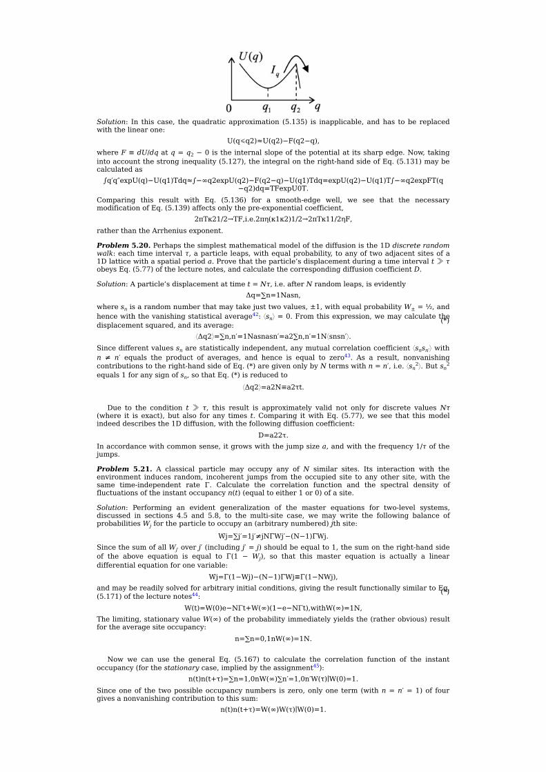
Solution: In thiscase, thequadraticapproximation (5.135) is inapplicable,andhas tobereplacedwiththelinearone:

U(q⩽q2)≈U(q2)−F(q2−q),whereF≡dU/dqatq=q2−0istheinternalslopeofthepotentialatitssharpedge.Now,takingintoaccountthestronginequality(5.127),theintegralontheright-handsideofEq.(5.131)maybecalculatedas

∫q′q″expU(q)−U(q1)Tdq≈∫−∞q2expU(q2)−F(q2−q)−U(q1)Tdq=expU(q2)−U(q1)T∫−∞q2expFT(q−q2)dq=TFexpU0T.

Comparing this result with Eq. (5.136) for a smooth-edge well, we see that the necessarymodificationofEq.(5.139)affectsonlythepre-exponentialcoefficient,

2πTκ21/2→TF,i.e.2πη(κ1κ2)1/2→2πTκ11/2ηF,ratherthantheArrheniusexponent.

Problem5.20.Perhapsthesimplestmathematicalmodelofthediffusionisthe1Ddiscreterandomwalk:eachtimeintervalτ,aparticleleaps,withequalprobability,toanyoftwoadjacentsitesofa1Dlatticewithaspatialperioda.Provethattheparticle’sdisplacementduringatimeintervalt≫τobeysEq.(5.77)ofthelecturenotes,andcalculatethecorrespondingdiffusioncoefficientD.

Solution:Aparticle’sdisplacementattimet=Nτ,i.e.afterNrandomleaps,isevidentlyΔq=∑n=1Nasn,

wheresnisarandomnumberthatmaytakejusttwovalues,±1,withequalprobabilityW±=½,andhencewiththevanishingstatisticalaverage42:⟨sn⟩=0.Fromthisexpression,wemaycalculatethedisplacementsquared,anditsaverage:

⟨Δq2⟩=∑n,n′=1Nasnasn′=a2∑n,n′=1N⟨snsn′⟩.Sincedifferentvaluessnarestatisticallyindependent,anymutualcorrelationcoefficient⟨snsn′⟩withn ≠ n′ equals the product of averages, and hence is equal to zero43. As a result, nonvanishingcontributionstotheright-handsideofEq.(*)aregivenonlybyNtermswithn=n′,i.e.⟨sn2⟩.Butsn2

equals1foranysignofsn,sothatEq.(*)isreducedto⟨Δq2⟩=a2N≡a2τt.

Due to the condition t≫ τ, this result is approximately valid not only for discrete valuesNτ

(where it isexact),butalso forany times t.Comparing itwithEq. (5.77),wesee that thismodelindeeddescribesthe1Ddiffusion,withthefollowingdiffusioncoefficient:

D=a22τ.Inaccordancewithcommonsense,itgrowswiththejumpsizea,andwiththefrequency1/τofthejumps.

Problem 5.21. A classical particle may occupy any of N similar sites. Its interaction with theenvironment induces random, incoherent jumps from theoccupiedsite toanyother site,with thesame time-independent rate Γ. Calculate the correlation function and the spectral density offluctuationsoftheinstantoccupancyn(t)(equaltoeither1or0)ofasite.

Solution: Performing an evident generalization of the master equations for two-level systems,discussed in sections 4.5 and 5.8, to the multi-site case, we may write the following balance ofprobabilitiesWjfortheparticletooccupyan(arbitrarynumbered)jthsite:

Wj=∑j′=1j′≠jNΓWj′−(N−1)ΓWj.SincethesumofallWj′overj′(includingj′=j)shouldbeequalto1,thesumontheright-handsideof the above equation is equal to Γ(1 − Wj), so that this master equation is actually a lineardifferentialequationforonevariable:

Wj=Γ(1−Wj)−(N−1)ΓWj≡Γ(1−NWj),andmaybereadilysolvedforarbitraryinitialconditions,givingtheresultfunctionallysimilartoEq.(5.171)ofthelecturenotes44:

W(t)=W(0)e−NΓt+W(∞)(1−e−NΓt),withW(∞)=1N,Thelimiting,stationaryvalueW(∞)oftheprobabilityimmediatelyyieldsthe(ratherobvious)resultfortheaveragesiteoccupancy:

n=∑n=0,1nW(∞)=1N.

Now we can use the general Eq. (5.167) to calculate the correlation function of the instantoccupancy(forthestationarycase,impliedbytheassignment45):

n(t)n(t+τ)=∑n=1,0nW(∞)∑n′=1,0n′W(τ)∣W(0)=1.Sinceoneof thetwopossibleoccupancynumbers iszero,onlyoneterm(withn=n′=1)of fourgivesanonvanishingcontributiontothissum:

n(t)n(t+τ)=W(∞)W(τ)∣W(0)=1.

Usingthegeneralsolution(*)withthereplacementoftwithτ,andW(0)=1,wegetn(t)n(t+τ)=1Ne−NΓτ+1N(1−e−NΓτ)≡1N1N+1−1Ne−NΓτ.

Asasanitycheck,aparticularcaseofthisresult,n(t)n(t)≡⟨n2⟩=1N,

maybereadilyverifiedbyasimplercalculation:⟨n2⟩=∑n=1,0n2W∞=1N.

Nowwearereadytocalculatethecorrelationfunctionoftheoccupancyfluctuations:

Kn(τ)≡n˜(t)n˜(t+τ)≡n(t)−nn(t+τ)−n=n(t)n(t+τ)−n2=1N1N+1−1Ne−NΓτ−1N2≡N−1N2e−NΓτ,andusetheWiener–Khinchintheorem(5.58)tofindtheirspectraldensity:

Sn(ω)=1πRe∫0+∞Kn(τ)eiωτdτ=N−1πN2Re∫0+∞e(−NΓ+iω)τdτ=N−1πN2Re1−NΓ+iω≡N−1πNΓNΓ2+ω2.

Theresultdescribesazero-frequency-centeredLorentzian line (typical forsuchproblems—see,

e.g.thetwo-stateproblemsolvedinsection5.8ofthelecturenotes),withthecut-offfrequency(i.e.thefluctuationbandwidth)NΓ.Asanadditionalsanitycheck,itshowsthatforasystemconsistingofjust one site (N = 1),Sn(ω) = 0, i.e. the site occupancy does not fluctuate—of course. As a lessobviouscorollary,thelow-frequencyfluctuationintensity

Sn(0)=1πΓN−1N3,asafunctionofN,reachesitsmaximumalreadyfortwositesandthendecreases.

NotealsothatfortheparticularcaseN=2,theresult isapplicabletotheEhrenfest’sdog-fleasystem(seeproblem2.1)with justone flea.However, in thiscasetheentropydoesnotchange intime,becauseithasthelargestpossiblevalueS=lnN=ln2fromtheverybeginning.

References[1]BurgessR1973Phys.Lett.A4437[2]LaxM1968FluctuationandCoherentPhenomenainClassicalandQuantumPhysics(GordonandBreach)[3]LouisellW1990QuantumStatisticalPropertiesofRadiation(Wiley)[4]VystavkinAetal1974Rev.Phys.Appl.979

1Forthesumcalculation,thewell-knownEq.(A.8b)isused.2HereEq.(A.9a)isusedforthesumcalculation.3Note that these twocasesmaybeconsideredas thenon-interacting limitsof, respectively, theIsingmodel (4.23)and theclassical limitof theHeisenbergmodel(4.21),whoseanalysiswithintheWeissapproximationwasthesubjectofproblem4.18.4See,e.g.sections1.1and4.5ofthelecturenotes,inparticularEq.(1.3),andthediscussionleadingtoEq.(4.90).5Notethatforasysteminanexternalfield,whichmayhaveη≡⟨sk⟩≠0,amoreappropriatedefinitionofthecorrelationcoefficient(whichensuresitsdecayat∣k−k′∣→∞)isKs≡⟨s˜ks˜k′⟩≡⟨sksk′⟩−⟨sk⟩⟨sk′⟩.6ThisresultisalsovalidforaclosedIsingring,butonlyifthesitedistancenismuchsmallerthanring’slengthN.(ThisiswhyforaringwithN=3,consideredofthepreviousproblem,Eq.(****)givesthecorrectresultonlyinthelimitJ≪T,whenstrongfluctuationssuppressthedifferencebetweenopenstringsandclosedrings.)ForauniformringwithN≫1sites,thegeneralexpressionforKsmaybecalculated(evenforh≠0)usingthetransfermatrixapproachdiscussedinsection4.5ofthelecturenotes;fordetailssee,e.g.section5.3inthebookbyYeomans,citedinthelecturenotes.7Thatformulawasfirstobtainedasearlyasin1909byAEinsteinfromthePlanck’sradiationlaw(whichdoesnottakethegroundstateenergyintoaccount),andisreproducedinsometextbookswithoutproperqualification.Noteagainthatthegroundstateenergyisnotonlymeasurable,butalsoresponsibleforseveralimportantphenomena—seethediscussioninsection2.6ofthelecturenotes.8See,e.g.Eq.(A.36e)withn=1.9NotethatEq.(**)fortheforceimposedbyasinglemolecule,whichwasprovedabove,doesnotmeanthatδP≪⟨P⟩.Indeed,duetotheindependenceofmolecularhits, ,while ,sothatfortheusual‘astronomical’valuesN∼1023,theratioδP/⟨P⟩∝1/N1/2ismuchsmallerthan1.10See,e.g.[1]andreferencestherein.Inbrief,the‘thermodynamic’derivationimpliesacontinuous,uniformspreadofthemomentum , transferred fromeachparticletothepistonduringonehit,overallthetimeperiodΔt=2L/∣v∣betweentheadjacenthits.Suchaspreadcouldbeachieved,forexample,byreplacingtheusualhardpistonwithaconducting,voltage-biasedlid,inducinganelectricfieldthatwouldpresschargedparticlesofthegastotheoppositelidofthecylinder.Iamnotawareofanypracticalimplementationofsuchasystem.11See,e.g.either[2]or[3].12Thisproblem,conceptually important for thequantummechanicsofopensystems,wasoffered inchapter7PartQMof thisseries,and is repeatedhere for thebenefitofreaderswho,foranyreason,skippedthatcourse.13See,e.g.PartCM section6.4, inparticularEq. (6.40),with ,andanarbitraryconstantd.Due to the linearityof thisequation,valid foreachCartesiancomponentofthe2Dvectorq(z,t),itisvalidforthevectorasthewholeaswell.14Thequantitativeconditionofthissmallnessis∣∂q(z,t)/∂z∣≪1.Forthermalfluctuations,inreal-lifeconditions,thisrequirementisalwayssatisfied.15Thisconditionisquiterealisticifthewavespropagatewithsomeattenuation—see,e.g.PartCMsection6.6.(Ifthisattenuationisnonvanishingbutnottoohigh,itdoesnotaffecttheforthcomingfluctuationanalysis.)16See,e.g.PartCMEqs.(6.45)and(6.47).17This result should not be too surprising, because the support point’smotion induces travelingwaves of the string,which carry away from it (‘to infinity’) themechanicalpower —see.e.g.PartCMEq.(6.49).18Thisproblem,forthecaseofarbitrarytemperature,wasthesubjectofPartQMproblem7.6,withproblem5.15ofthatpartservingasthebackground.However,themethodusedinthemodelsolutionsofthoseproblemsrequiresonetoprescribe,totheoscillators,differentfrequenciesω1andω2atfirst,andonlyafter thismoregeneralproblemhasbeensolved,pursuethelimitω1→ω2.ThegoalofthisproblemistodemonstratethattheLangevinformalismenablesasolutiontakingω1=ω2≡ω0fromtheverybeginning.19See,e.g.PartEMEq.(3.16),inwhichthedipolemomentsaredenotedasp1,2.20See,e.g.PartEMEq.(3.13).Inthesecondformofthisexpression,thez-axisisassumedtobedirectedalongthevectorr.21See,e.g.PartEMEq.(3.15b).Notethefactors½,whichareduetotheinducednatureofthemomentsd˜2,1.22Actually,itmaybereadilyworkedoutbydifferentiation,overaparameter,ofthefollowing(generallyuseful)tableintegral:

∫0∞dξ(aξ)2+2bξ+1=π23/2(a+b)1/2,fora+b>0,butIdidnotwanttodistractthereader’sattentionfromphysics.23Thisisaveryusefuladditionalexercise,highlyrecommendedtothereader.24See,e.g.PartCM sections 5.2–5.5.Note that in quantummechanics, a similar approach is called the rotating-waveapproximation (RWA)—see, e.g.Part QMsections6.5,7.6,9.2,and9.4.25Here,incontrasttoPartCMsection5.4,capitallettersΩandΩ0areisusedtodenotethefrequenciesofthephaselockingforceandtheoscillator,todistinguishthemfromfrequenciesωoftheFouriercomponentsoffluctuations.26See,e.g.PartCMEq.(5.41).Inthisapproximation,theoscillationamplitudeA(t)maybeconsideredconstant—seePartCMEq.(5.71)anditsdiscussion.27See,e.g.thesecondofPartCMEqs.(4.57a).28Forourcurrentautonomouscase,withΔ=0,thisapproximationisvalidifthespectraldensitySf(ω)ofthenoiseisvirtuallyconstantinafrequencyinterval(around

theself-oscillationfrequencyΩ0)thatislargerthantheoscillationlinewidthwearecurrentlycalculating—seebelow.29See,e.g.Eq.(A.2a)withn=−N/Γτ.30NotethatthiscalculationessentiallyrepeatsthederivationofEq.(7.89)inPartQMsection7.3.Thisisnatural,becausethequantumstatedephasing,describedinthatsection,isessentiallythedecoherenceofthefundamentaloscillationsofthequantum-mechanicalwavefunctionintime(withfrequencyE/ℏ),undertheeffectoflow-frequencyexternalfluctuationsimposedbytheenvironment.31See,e.g.briefdiscussionsinPartEMsection6.5andPartQMsections1.6and2.8.32Justforthereader’sreference:Suchagradualdestructionofphaselocking,describedwithintheframeworkofEq.(***),isoneofmostfamousanalyticallysolvablenonlinearproblemsofthefluctuationtheory.Thissolution,firstfoundin1958byRStratonovichandthenrepeatedlyre-discoveredbyothers,maybeexpressedeitherviasomeexoticBesselfunctions(ofanimaginary,continuousorder),orasaseriesincludingthe‘usual’modifiedBesselfunctionsIk(ofanintegerorderk),orjustasthesolutionofaverysimplesystemoflinearalgebraicequations—see,e.g.section2in[4].33Ifyouneedto,seeEq.(A.32a).34Pleasenoteagainthat,aswasnotedatthederivationofthatresult,thedirectstatisticalaverageofthenoise-inducedoscillationsq(t)yieldsexactzero,sothatthecorrelationfunctionisthesimplestquantitativetime-domaincharacteristicofthenoise-inducedrandomoscillations.35Notethatthisdiscussionisvalidforthegeneral(quantum)case,ℏω∼T,onlyifbothKq(τ)andSq(ω)areunderstood in thesenseof thesymmetrizedfunctionsdefinedbyEqs.(5.95)–(5.96).36See,e.g.Eq.(A.38).37See,e.g.PartEMsection7.6.38See,e.g.PartEMsections4.1and6.6.39Bytheway,thisequivalentcircuitgivesanalternativewaytoderiveEq.(5.81c)ofthelecturenotes.Indeed,iftheresistorisconnectedtoanidealammeter(withzerointernalresistance),weseethatthevoltage vanishes,whilethefluctuationcurrentbecomesequalto ,withthevariance

TogetherwithEq.(5.81b),thisrelationimmediatelygivesEq.(5.81c).40See,e.g.PartEMsection7.6.41Bytheway,thisisexactlythewayHNyquistfirstderivedhistheorem—correctlyfortheclassicallimitℏω≪Tandwitha‘small’errorforthegeneral(quantum)case.ThiserrorwascorrectedlaterbyHCallenandTWelton,whousedadifferentapproach(andconsideredamoregeneralsituation).42Thisprocessisevidentlymemory-free,i.e.ergodic,sothatthisaveragingmaybeunderstoodaseitherthatovertheensembleofmanydifferentrandomwalks,orovertheensembleofleapsinasinglewalkwithN≫1steps.43Notethatthesimilarargumentwasusedinsection5.1ofthelecturenotestoderiveEq.(5.12).44Itisevidentthatinthisuniformsystemalltheresultsareindependentofthesitenumber,sothatfromthispointontheindexjisdropped.45Note again the somewhat counter-intuitive nature of Eq. (5.167): it expresses an average for a stationary process via the probability evolution laws for non-stationarycase(withspecialinitialconditions).

(**)

(*)

IOPPublishing

StatisticalMechanicsProblemswithsolutionsKonstantinKLikharev

Chapter6

Elementsofkinetics

Problem6.1.UsetheBoltzmannequationintherelaxation-timeapproximationtoderivetheDrudeformulaforthecomplexacconductivityσ(ω),andgiveaphysicalinterpretationoftheresult’strendathighfrequencies.

Solution: For a uniform system, in a uniformly distributed ac field , in the Boltzmann equation(6.18)wemayneglectthetermproportionalto∇rw,buthavetoretaintheterm∂w/∂t.Then,inthesamelow-fieldapproximationaswasusedtoderiveEq.(6.25),wegetthefollowinggeneralizationtotime-dependentcases:

Lookingforthevariables andw˜assinusoidalfunctionsoftime(proportionaltoexp{−iωt}),wegetfromEq.(*)thefollowingrelationbetweentheircomplexamplitudes:

ComparingthisresultwithEqs.(6.25),weseethattheonlychangeduetothenon-zerofrequencyωisthefactor(1−iωτ)inthedenominatorofexpressionsfortheprobabilityperturbation,andhenceforthecomplexamplitudejωoftheelectriccurrent j,givenbyEq. (6.26).Hence, thesamefactorappears in the complex conductivityσ(ω), defined by a relation similar to Eq. (6.28), but for thecomplexamplitudesjωand :

whereσ(0)isgivenbyEq.(6.29)—andhencebytheDrudeformula(6.32).Forthepurposeofinterpretation,letusrewritethisresultas

σ(ω)=σ′(ω)+iσ″(ω),withσ′(ω)=σ(0)1+(ωτ)2,σ″(ω)=σ(0)ωτ1+(ωτ)2.It shows that the real part σ′ of the conductivity, responsible in particular for the Joule heatgeneration,dropsfastassoonasthefieldfrequencyexceedsthereciprocalrelaxationtime1/τ(inpractical conductors, from ∼1011 to ∼1013 s−1), while its imaginary part σ″ first grows withfrequency, and then starts dropping as well, but slower, as 1/ωτ. The latter behavior, with τ-independentimaginaryconductivity

σ″(ω)≈σ(0)ωτ≡q2nmω,atωτ≫1,correspondstocollision-freeoscillationsofparticledisplacements,inducedbytheexternalacfield.

Nownotethatthefrequencydependenceofthecurrentdensityatωτ≫1issimilartothatofthecurrent in a lumped inductance L (with voltage , and hence ). Due to thissimilarity, the σ″ given by Eq. (**) is called the kinetic inductance of a conductor, because, incontrast to the usual ‘magnetic’ inductance, it is due to the finite massm (inertia) of the chargecarriers, rather than the magnetic field it induces. This effect is especially noticeable insuperconductors,whoselinearelectrodynamicsmaybeapproximatelydescribedasthatoftheusualconductors,butwithnegligiblescattering, i.e.withτ=∞,sothatEq.(**),withnandmreplacedwithcertaineffectiveparameters,isvalidinaverybroadrangeoffrequenciesstartingfromzero1.

Problem 6.2. Apply the variable separation method2 to the drift–diffusion equation (6.50) tocalculate the time evolution of the particle density distribution in an unlimited uniform medium,providedthatatt=0,theparticlesarereleasedfromtheiruniformdistributioninaplanelayerofthickness2a:

n=n0,for−a⩽x⩽+a,0,otherwise.Solution: In the absence of a drift-inducing field, ∇U = 0, the drift–diffusion equation (6.50) isreducedtothesimplediffusionequationsimilartoEq.(5.116),

∂n∂t=D∇2n,withD=τTm.Thisequationisisotropic,sothattheinitial1Ddistributionn=n(x,0)remainsone-dimensionalatalllatertimes,anditsevolutionmaybedescribedbythe1Dversionofthediffusionequation:

∂n∂t=D∂2n∂x2.

(**)

(***)

(****)

(*)

Letuslookforthesolutionofthisequationinthevariable-separatedformnx,t=∑kTktXkx.

Plugging a particular term of this series into Eq. (*), and dividing both parts of the equation byDTkXk,weget

1DTkdTkdt=1Xkd2Xkdx2=const≡−k2.SolvingthetworesultingsimpleordinarydifferentialequationsforTkandXk,weget

Tk=akexp{−Dk2t},Xk=bkcoskx,with (so far) arbitrary ak and bk.3 Since the length of the diffusion segment (−∞ ⩽ x ⩽ + ∞) isinfinite,thespectrumofeigenvalueskiscontinuous,sothatpluggingthesesolutionsintoEq.(**),weneedtoreplacethesummationoverkwithintegration:

nx,t=∫−∞+∞ckexp{−Dk2t}coskxdk,whereck≡akbk.

Whatremainsistofindthefunctionckfromtheinitialcondition(att=0):∫−∞+∞ckcoskxdk≡12∫−∞+∞ck(eikx+e−ikx)dk=nx,0≡n0,for−a⩽x⩽+a,0,otherwise.

AsusualforthereciprocalFouriertransform,letusmultiplybothpartsofthisequationbye−ik′x,andintegratetheresultoverthewholex-axis.Changingtheorderof integrationontheleft-handside,weget

12∫−∞+∞dkck∫−∞+∞dx[ei(k−k′)x+ei(k+k′)x]=∫−∞+∞n(x,0)e−ik′xdx≡n0∫−a+acosk′xdx.The inner integral on the left-hand side equals 2π[δ(k − k′) + δ(k + k′)],4 so that the outerintegrationiseasy,giving

12(ck′+c−k′)=n02π∫−a+acosk′xdx≡n0πsink′ak′.

AccordingtoEq.(***),ck′hastobeanevenfunctionofk′,sothat(droppingtheprimesignatk),thisresultbecomes

ck=n0πsinkak,andpluggingitintoEq.(***),wemayfoldtheintegralinthatformulatothepositivesemi-axis.Asaresult,weget

nx,t=2n0π∫0+∞exp{−Dk2t}sinkakcoskxdk.

Plots of this distribution for several values of the normalized time , where , are

showninthefigureabove.Theplotsshowthattheinitiallyrectangulardistributionoftheparticledensityfirstsmearsattheedgesveryfast,butthelater(at )spreadoftheparticlesbecomesslowerandslowerwithtime.Thisisverynaturalinthelightofthebasiclaw(5.77)ofdiffusionofasingle particle (equivalent to the delta-functional initial distribution ofn), in our current notationreading

δx=2Dt1/2.Reversing thesamestatement into the timedomain,wemaysay that thecharacteristic timeofasubstantialchangeoftheparticledistributionisnot ,butratherΔt∼(Δx)2/D,whereΔxisthespatialwidthofthesharpfeature(s)ofthedistribution.(At ,thisisthefullwidthΔx≫aofthewholedistribution,sothat .)

Problem6.3.SolvethepreviousproblemusinganappropriateGreen’sfunctionforthe1Dversionofthediffusionequation,anddiscusstherelativeconvenienceoftheresults.

Solution: The spatial–temporal Green’s function of any linear, homogeneous, partial differentialequationin1+1dimensions(1coordinate+time)maybedefinedbythefollowinggeneralformulaforthesolutionoftheequationatt>t0:

nx,t=∫−∞+∞n(x0,t0)G(x,t;x0,t0)dx0.Appliedtothedelta-functionalinitialconditions,thisdefinitionyields

n(x,t)=G(x,t;x0,t0),ifn(x,t0)=δ(x−x0).

(**)

Butsuchasolution(witht0=0)ofthediffusionequation,givenbyEq.(*)ofthepreviousproblem,andequivalenttoEq.(5.114)ofthelecturenotes,

∂n∂t=D∂2n∂x2,for−∞<x<+∞,wasalreadydiscussedinsection5.6—seeEqs.(5.112)and(5.113).Fromtheserelations,

G(x,t;x0,t0)=12π1/2δxtexp−(x−x0)22δxt2,withδxt=2D(t−t0)1/2,sothatEq.(*),witht0=0,becomes

nx,t=14πDt1/2∫−∞+∞n(x0,0)exp−(x−x0)24Dtdx0.

Fortheinitialconditionsspecifiedinthepreviousproblem,nx,0=n0,for−a⩽x⩽+a,0,otherwise,

wegetnx,t=n04πDt1/2∫−a+aexp−(x−x0)24Dtdx0.

This integral may be readily expressed via a difference of two values of the so-called error

functionerfζ≡2π1/2∫0ζexp{−ξ2}dξ;

however, for most practical purposes the explicit integral form (**) is preferable. In particular, ityields exactly the same plots of function n(x, t) as shown in the model solution of the previousproblem—despitethesubstantialdifferenceoftheexpressionforms.Indeed,theresult(****)oftheprevious problem is just the Fourier-integral expansion of Eq. (**). However, for practicalcalculations, there isabigdifferencebetweenthesetwo integral forms: thereal-space integral inEq.(**)convergesfasteratrelativelysmalltimes, whilethereciprocal-spaceintegral,obtainedfromthevariableseparation,convergesfasterat ,whenonlyrelativelysmallvaluesoftheeffectivewavenumberk,with∣k∣∼1/(Dt)1/2≪1/a,givenoticeablecontributionsintoit.

Problem6.4.*Calculatethedcelectricconductanceofanarrow,uniformconductinglinkbetweentwo bulk conductors, in the low-voltage and low-temperature limit, neglecting the electroninteractionandscatteringinsidethelink.

Solution: As was discussed in section 3.3 of the lecture notes, atT → 0 any fermions (includingelectrons) in equilibrium fill all eigenstates up to the Fermi energy εF. As we know from thediscussioninsection6.3(see,inparticular,figure6.5c),ifconductorsareweaklyconnected,withnovoltageappliedbetweenthem,theirFermilevelsbecomealigned.Thedcvoltage appliedbetweentwoconductorsshiftsalltheirenergyspectraby ,sothatthesingle-particleenergydiagramofthewholesystemlooksassketchedinthefigurebelow.

Let us assume that the link is uniform5; then in the absence of scattering, the longitudinal

componentεxoftheelectron’senergyisconserved.Inthiscase,asthefigureaboveshows,itcanmovefromconductor1toconductor2onlyifthisenergyiswithintherange6

whereε⊥ istheeigenenergycorrespondingtothetransversecomponentψ⊥(y,z)ofthestationaryorbitalwavefunction

ψr=aψ⊥y,zexp{ikxx},sothatthefullenergyoftheelectronisεx+ε⊥,where

εx=ℏ2kx22m.

If theappliedvoltage is low, , thenumberNofdifferentelectronstateswith thesametransversewavefunctionψ⊥(y,z),maybecalculatedas

where the front factor of 2 is due to two possible electron spin states with the same ‘orbital’wavefunctionψ(r),whiledN/dεxisthe1Ddensityoftheorbitalstates,whichmaybecalculatedas7

dNdεx=dNdkx/dεxdkx≡l2π/dℏ2kx2/2mdkx≡l2π/ℏ2kxm≡l2π/21/2ℏεx1/2m1/2.Withthisresult,Eq.(*)becomes

(***)

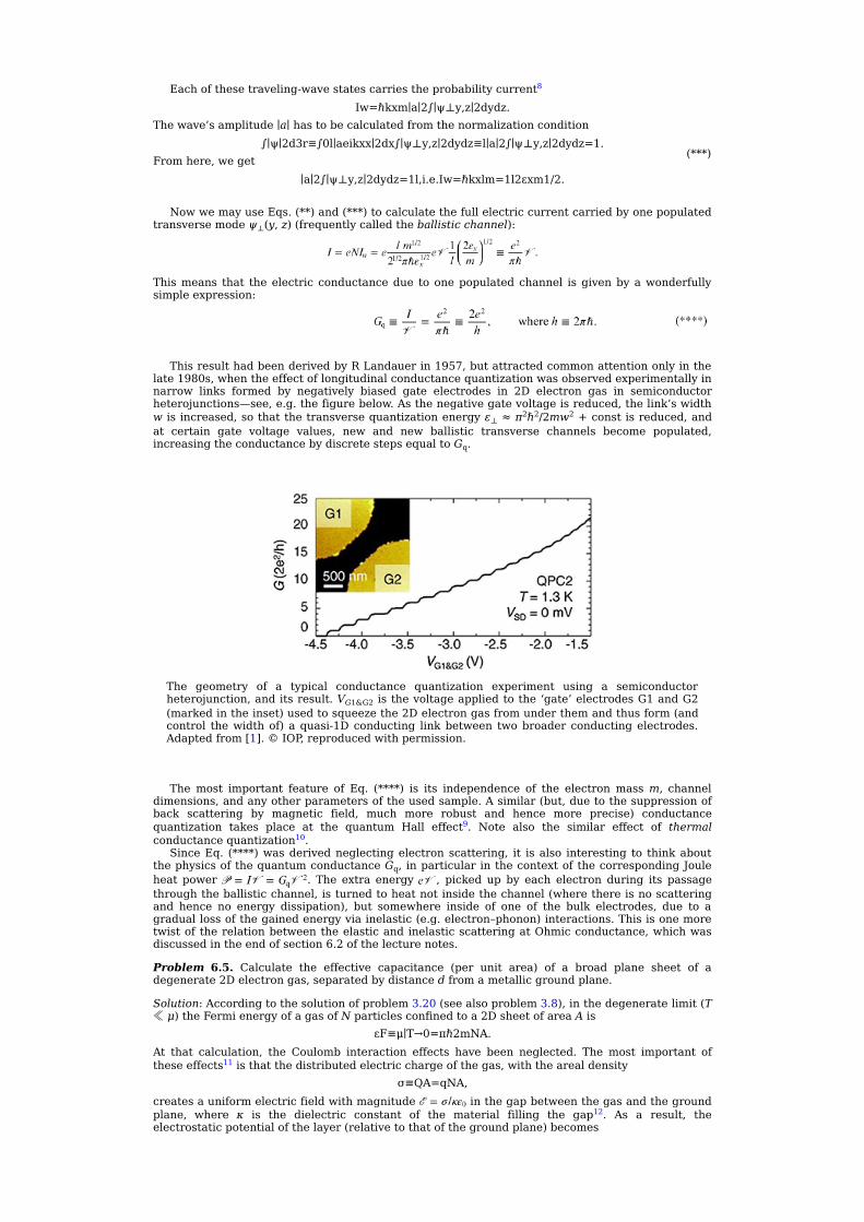
Eachofthesetraveling-wavestatescarriestheprobabilitycurrent8

Iw=ℏkxm∣a∣2∫∣ψ⊥y,z∣2dydz.Thewave’samplitude∣a∣hastobecalculatedfromthenormalizationcondition

∫∣ψ∣2d3r≡∫0l∣aeikxx∣2dx∫∣ψ⊥y,z∣2dydz≡l∣a∣2∫∣ψ⊥y,z∣2dydz=1.Fromhere,weget

∣a∣2∫∣ψ⊥y,z∣2dydz=1l,i.e.Iw=ℏkxlm=1l2εxm1/2.

NowwemayuseEqs.(**)and(***)tocalculatethefullelectriccurrentcarriedbyonepopulatedtransversemodeψ⊥(y,z)(frequentlycalledtheballisticchannel):

Thismeans that theelectricconductancedue toonepopulatedchannel isgivenbyawonderfullysimpleexpression:

ThisresulthadbeenderivedbyRLandauerin1957,butattractedcommonattentiononlyinthe

late1980s,whentheeffectoflongitudinalconductancequantizationwasobservedexperimentallyinnarrow links formed by negatively biased gate electrodes in 2D electron gas in semiconductorheterojunctions—see,e.g.thefigurebelow.Asthenegativegatevoltageisreduced,thelink’swidthwisincreased,sothatthetransversequantizationenergyε⊥≈π2ℏ2/2mw2+constisreduced,andat certain gate voltage values, new and new ballistic transverse channels become populated,increasingtheconductancebydiscretestepsequaltoGq.

The geometry of a typical conductance quantization experiment using a semiconductorheterojunction,anditsresult.VG1&G2isthevoltageappliedtothe‘gate’electrodesG1andG2(markedintheinset)usedtosqueezethe2Delectrongasfromunderthemandthusform(andcontrol thewidthof)aquasi-1Dconducting linkbetweentwobroaderconductingelectrodes.Adaptedfrom[1].©IOP,reproducedwithpermission.

The most important feature of Eq. (****) is its independence of the electron massm, channeldimensions,andanyotherparametersoftheusedsample.Asimilar(but,duetothesuppressionofback scattering by magnetic field, much more robust and hence more precise) conductancequantization takes place at the quantum Hall effect9. Note also the similar effect of thermalconductancequantization10.

SinceEq. (****)wasderivedneglectingelectronscattering, it isalso interestingto thinkaboutthephysicsofthequantumconductanceGq,inparticularinthecontextofthecorrespondingJouleheat power . The extra energy , picked up by each electron during its passagethroughtheballisticchannel,isturnedtoheatnotinsidethechannel(wherethereisnoscatteringand hence no energy dissipation), but somewhere inside of one of the bulk electrodes, due to agraduallossofthegainedenergyviainelastic(e.g.electron–phonon)interactions.ThisisonemoretwistoftherelationbetweentheelasticandinelasticscatteringatOhmicconductance,whichwasdiscussedintheendofsection6.2ofthelecturenotes.

Problem 6.5. Calculate the effective capacitance (per unit area) of a broad plane sheet of adegenerate2Delectrongas,separatedbydistancedfromametallicgroundplane.

Solution:Accordingtothesolutionofproblem3.20(seealsoproblem3.8),inthedegeneratelimit(T≪μ)theFermienergyofagasofNparticlesconfinedtoa2DsheetofareaAis

εF≡μ∣T→0=πℏ2mNA.At that calculation, the Coulomb interaction effects have been neglected. The most important oftheseeffects11isthatthedistributedelectricchargeofthegas,withthearealdensity

σ≡QA=qNA,createsauniformelectricfieldwithmagnitude inthegapbetweenthegasandthegroundplane, where κ is the dielectric constant of the material filling the gap12. As a result, theelectrostaticpotentialofthelayer(relativetothatofthegroundplane)becomes

(*)

(*)

(**)

(***)

sothattheelectrochemicalpotential(6.40)ofthelayerbecomesequaltoμ′≡qϕ+μ=q2dκε0NA+πℏ2mNA≡σqdκε0+πℏ2mq2.

Aswasdiscussed in section6.3, thenetelectrochemicalpotentialμ′ (dividedbyq) iswhatwe

usuallymeasureasthevoltage , inthiscasebetweentheelectrongasandthegroundplane.Aswe know from the elementary electrostatics, capacitance C is just the ratio , so that thecapacitanceperunitarea(C/A)istheratio ,andEq.(*)mayberepresentedas

CA−1=dκε0+πℏ2mq2.In thecircuit theory language, thismeans that theeffectivecapacitanceC of the2Delectrongassheetisaconnection,inseries:

1C=1Ce+1Cq,oftheusual,‘electrostatic’capacitance

Ce=κε0dA,andtheso-calledquantumcapacitance13

Cq=mq2πℏ2A.

Thephysicsofthiseffectisprettystraightforward:byitsdefinition,theelectrochemicalpotentialis the average energynecessary to addoneparticle from the environment (in our case, from theground plane) to the system. In our case such addition requires, first, to overcome the Coulombrepulsionoftheelectronsalreadyinthesheetand,second,togivetoonemoreparticletheFermienergyofthegasεFtofillthelowestquantumstatenotyetoccupied—justaboveεF.Inthesimplemodelanalyzedabove, theseenergyadditionsare independent, leading to theadditionof the twocontributionstotheeffectivepotentialμ′,andhencetotheadditionofthereciprocalcapacitancesdescribingeachoftheenergycomponents.

Forfreeelectrons(with ∣q∣=e≈1.6×10−19Candm=me≈0.91×10−30kg), thequantumcapacitance is quite macroscopic, Cq/A ≈ 0.67 F m−2, and becomes even smaller (so that theimportantfraction1/Cqbecomeslarger)insemiconductorswithlowereffectiveelectronmass—e.g.m≈0.2me in the conduction band of Si. Because of that, its effects may be noticeable in somemodern electron devices—most importantly, in the ubiquitous silicon field-effect transistors withtheirverythingateinsulatinglayers.(ForcomparisonwiththeaboveestimateofCq/A,theratioCe/Aformodernhigh-κgate-oxidelayersmaybeoftheorderof0.1Fm−2.)

Problem 6.6. Give a quantitative description of the dopant atom ionization, which would beconsistentwiththeconductionandvalencebandoccupationstatistics,usingthesamesimplemodelofann-dopedsemiconductorasinsection6.4ofthelecturenotes(seefigure6.7a),andtakingintoaccountthatthegroundstateofthedopantatomistypicallydoublydegenerate,duetotwopossiblespin orientations of the bound electron. Use the results to verify Eq. (6.65), within the displayedlimitsofitsvalidity.

Solution:Forspellingouttheelectroneutralitycondition(6.62),n=p+n+,

we need to express the concentrations n,p, and n+ via the parameters μ andT (in equilibrium,common for all components of the system), at the given energies εV,εC, andεD—see figure 6.7a,reproducedbelow.Aswasarguedinsection6.4ofthelecturenotes,atT≪Δ≡εC−εV,Eqs.(6.58),

n=nCexpμ−εCT,p=nVexpεV−μT,

are independent of thedopant excitation statistics, soweneedonly to express thenumbern+ ofactivated (ionized) dopants via the above parameters and the full concentrationnD of thedopantatoms.

This may be done similarly to the calculation ofN0 in the solution of problem 3.9.14 With theassumptiongivenintheassignment,thedonoratommaybeineitherofthreedifferentstates:oneionizedstate,withoutanelectron,withacertainenergyεa,andanyoftwogroundstates,withoneelectronofanyspinorientation,andwiththeenergyεa+εD.ApplyingthegeneralEqs.(2.106)and(2.107)toagrandcanonicalensembleofsuchsystems,forthecorrespondingprobabilitieswemaywrite

W0=1ZGexp−εaT,W1=1ZGexpμ−(εD+εa)T,with

ZG=exp−εaT+2expμ−(εD+εa)T≡exp−εaT1+2expμ−εDT,sothattheprobabilitiesW0,1areindependentofεa(astheyshouldbe):

W0=11+2exp(μ−εD)/T,W1=exp(μ−εD)/T1+2exp(μ−εD)/T.Fromhere,theaveragenumberofionizedatoms(perunitvolume)is

(****)

n+=nDW0=nD1+2exp(μ−εD)/T.Asasanitycheck,Eq.(***)showsthatatfixedμandT,thefractionn+/nDof theactivateddonorsincreasesasεDisincreased—asitshouldaccordingtotheenergydiagramshownabove.

Withthisexpression,theelectroneutralitycondition(*)takestheformnCexpμ−εCT=nVexpεV−μT+nD1+2exp(μ−εD)/T.

Generally, this transcendental equation for μ cannot be solved analytically. However, it may bereadilyusedtoplottheelectrondensityn,givenbythefirstofEqs.(**),asafunctionofnD,withthechemicalpotentialμusedastheparameter—seethesolidredlineinthefigurebelow,calculatedforparameterstypicalforsemiconductors.(Notethelog–logscaleoftheplot,coveringmanyordersofmagnitudeofbothdensities.)

TheplotshowsthatatT≪Δ,therearethreedistinctbranchesofnasafunctionofthedopant

densitynD.

(i) If the density is very low, nD ≪ ni,15 the last term in Eq. (****) is negligible, so that thesemiconductor remainspractically intrinsic,withn≈p≈ni, and the chemical potential near themidgap:μ≈(εC+εV)/2.

(ii)Inthe(mosttypical)casewhennDisincreasedwellbeyondni,thenumbern+ofactivatedatomsandtheelectrondensitynarevirtuallyequaltonD(andhencetemperature-independent),withthehole density p decreasing accordingly, and the chemical potential gradually rising toward theconductionbandedge—seeEqs.(6.65)ofthelecturenotes:

n≈nD,p≈ni2nD≪n,μ≈εC−TlnnCnD.

Note that this result means that the donor atoms may be fully activated even if the apparentionizationenergy(εC−εD)ismuchlargerthanT—asit isintheexampleshownintheplotabove.Themathematicalexplanationofthiscounter-intuitivefact isgivenbyEq.(***):whatis importantfor the full activation is theFermi levelμ tobewell (bya fewT) belowεD, andaccording toEq.(****),thevalueofμparticipating inthisexpressiondependsontheconductionandvalencebandstatisticsaswell.ThehandwavingphysicalinterpretationIcanofferisthatatnD≫ni,therelativelyabundantelectronswiththeenergyεDmayreadilygodowntotheFermilevel(playingtheroleofaneffectiveexternalparticlesource—cf. figure2.13of the lecturenotes)witha lowerenergyμ,andfromtherebere-distributedintotheconductionandvalencebands—mostlytotheformerone.Suchinterpretation of the Fermi level as a virtual reservoir of particles is generally useful for a semi-quantitativeanalysisofothersystemsaswell.

(iii)Finally,ifnDbecomessohighthattheμexpressedbyEq.(6.65)ofthelecturenotesenterstheT-widevicinityofthedopinglevelεD,thelastterminEq.(****)becomessomewhatlowerthannD,causing a proportional reduction ofn—see the deviation of the solid red line from the (straight)dashed one in the top right corner of the figure above. However, as the plot shows, for typicalparametervaluesthiseffectisrelativelyminor,andEq.(6.65)isvirtuallyprecisewithinmanyordersofmagnitude.

Problem6.7.Generalizethesolutionof thepreviousproblemtothecasewhenthen-dopingofasemiconductor is complemented with its simultaneous p-doping by nA acceptor atoms per unitvolume, whose energy εA − εV of activation, i.e. of accepting an additional electron and hencebecominganegativeion,ismuchlessthanthebandgapΔ—seethefigurebelow.

(*)

(**)

(***)

(****)

Solution:Inthiscase,theelectroneutralityconditionshouldalsotakeintoaccountthedensityn−ofnegativelyionizedacceptorions,becoming

n+n−=p+n+.Thedensityn−maybecalculatedjustliken+wascalculatedinthesolutionofthepreviousproblem,onlytakingintoaccountthedifferencebetweentheelectronsandholes.Theresultis16

n−=nA1+2exp(εA−μ)/T.Withthisexpression,andtheformulasforn,p,andn+giveninthesolutionofthepreviousproblem,Eq.(*)becomes

nCexpμ−εCT+nA1+2exp(εA−μ)/T=nVexpεV−μT+nD1+2exp(μ−εD)/T.

Thistranscendentalequationforμcannotbesolvedanalyticallyinthegeneralcase.However,itmay be used to plot, for example, the reciprocal dependence of the donor doping level nD, as afunctionoftheμityields,forseveralvaluesofnA—seethefigurebelow.

Theplotsclearlyshowthatat theusualconditionsT≪ΔandnD,nA≪nC,nV, there are three

distinctrangesofdoping,whereEq.(**)yieldssimpleresults:

(i) At nD ∼ nA, the value of μ is somewhere around the midgap, the exponents in the termsproportionaltonAandnDaremuchsmallerthan1(showingthatthedopantatomsofbothtypesarefullyactivated),andEq.(**)isreducedto

n+nA=p+nD.ThisequationissimilartoEq.(6.63)ofthelecturenotes,justwithnDreplacedwiththedifference(nD−nA).Withthisreplacement,itssolutionisgivenbyEq.(6.64):

n=nD−nA2+(nD−nA)24+ni21/2,p=nA−nD2+(nD−nA)24+ni21/2≡nni2,whereniistheintrinsiccarrierdensitynigivenbyEq.(6.60):

ni=(nCnV)1/2exp−Δ2T.Themostimportantfeatureofthisresultisthat

n−p=nD−nA,sothatthesignof(n−p),i.e.oftheeffectivechargeofcarriers,maybecontrolledbydoping.Suchcompensated semiconductors are convenient for some special applications, but in mostsemiconductordevices,oneofthefollowingtwolimitsisused.

(ii)Ifni,nA≪nD(butnDisstillmuchlowerthantheeffectivedensitynCofstatesintheconductionband),thesituationisreducedtothestrongn-dopinganalyzedinsection6.4ofthelecturenotes,whereEqs.(6.65)arevalid:

μ≈εC−TlnnCnD,n≈nD,p≈ni2nD≪n.The dashed straight line in the figure above shows the first of these approximate equalities. TherelativelyminordeviationsfromitinthetoprightcorneroftheplotsareduetothecloseapproachofμtoεD—seethepreviousproblem.

(iii)Intheoppositelimitofdominatingp-doping(ni,nD≪nA≪nV),Eq.(**)isreducedtotheequallysimpleEqs.(6.67)ofthelecturenotes:

μ≈εV+TlnnVnA,n≈nA,n≈ni2nA≪p,sothatthecarrierdensitiesandtheFermilevelinthiscasearevirtuallyindependentofnD—seetheleft,nearly-verticaltailsoftheplotsinthefigureabove17.

Problem 6.8. A nearly-classical gas of N particles with mass m, is in thermal equilibrium attemperatureT,inaclosedcontainerofvolumeV.Atsomemoment,anorificeofaverysmallareaAisopen inthecontainer’swall,allowingtheparticlestoescape intothesurroundingvacuum18. Inthelimitofverylowdensityn≡N/V,usesimplekineticargumentstocalculatethermsvelocityofthe escaping particles during the time when the number of escaped particles is still negligible.FormulatethelimitsofvalidityofyourresultsintermsofV,A,andthemeanfreepathl.

Solution:Assumingthe linearsizesof theorificearemuchsmaller thanthoseof thecontainer,sothatA≪V2/3,letuscalculatetheaveragevelocityoftheparticlesthathittheorificeareaduringatimeintervalΔt≫A1/2/ ,where ≡(3T/m)1/2istheirrmsvelocityinequilibrium—seeEq.(3.9)ofthelecturenotes.Forthat,letusalsoassumethat,simultaneously,Δtismuchlessthan ,sothattheparticle collisions at their path to the orificemaybeneglected; thenonly theparticles flyingdirectly toward the hole area may hit it—see the figure below. Moreover, the velocities of suchparticlesshouldsatisfythecondition ⩾r/Δt,whereristheinitialdistanceoftheparticlefromthehole.(Ifthelinearsizescaleoftheorifice,A1/2,ismuchlessthanthisr,itisnotimportantexactlywhichpartoftheholewearespeakingabouthere.)

Thenumberofsuchparticles,withvelocitieswithinasmallrange , isproportionalto

:

wheretheprobabilitydensityw( )obeystheMaxwelldistribution,

(Sincetheparticlesfromeachpointmayreachtheholeareaonlyiftheyflyinacertaindirection,thedistribution shouldbe for oneCartesian component of the velocity only.)As a result,wemaywrite

wherec is some ‘constant’—whichmaydependon theareaof theholeand thevelocitydirection.Now the average 2 of the molecules hitting the hole area, from a certain direction, may becalculatedas19

Thisresultdoesnotincludethevelocitydirection,andhenceisvalidforthewholeparticleflux.It

also is independent of the time interval Δt, but since particle collisions were neglected at itsderivation,itmaylooklikeitisonlyvalidforintervalswithintheinitiallyassumedrange

However,ifthelossofparticlesissufficientlysmall,asassumedintheassignment,theeffusiondoes

not change the statistical distribution of the particles, because their mutual scattering tends torestore it at each point. (The process is frequently called thermalization.) Hence Eq. (**) isapplicable to each sequential time interval after the orifice opening, even at t≫ A1/2/ . Note,howeverthattheinterval(***)disappearsiflisreducedtoapproachthescaleofthelinearsizesoftheorifice,A1/2.HencetheimportantconditionofvalidityofouranalysisisA1/2≪l.(Wehavealsoneglected possible reflections of the particles from the orifice area—the assumption correct inparticularifthewallthicknessismuchsmallerthanA1/2.)

NotethataccordingtoEq.(**),theescapingparticlesare,onaverage,hotterthanthegasasawhole:

Hencetheeffusiontendstocoolthegas,andthemaintenanceofitsthermalequilibriumwithfixedtemperatureTwouldrequireasupplyofheatfromanexternalsource.

Problem6.9.Forthesystemanalyzedinthepreviousproblem,calculatetherateofparticleflowthroughtheorifice(theso-calledeffusionrate).Discussthelimitsofvalidityofyourresult.

Solution:Letuscalculatetheeffusionrate,whichmaybedefinedasΓ≡−dNdt>0,

usingthesameballisticapproachasinthemodelsolutionofthepreviousproblem.Considerasmallgroupofparticleshavingacertainvelocityv,withangleθtothedirectionnormaltothewallwiththe orifice in it—see the figure below. The area dA′ of transverse displacements (normal to thevelocityvectorv),leadingtotheparticle’spassagethroughtheorifice,isAcosθ,whiletherangedrofradialdistances,leadingtosuchapassageduringasmalltimeintervaldt,isdr= ,sothatthenumberofsuchescapingparticlesis

wheren≡N/Visthespatialdensityoftheparticles,andw(v)isthe3DMaxwelldistribution,givenbyEqs.(3.5)and(3.6)ofthelecturenotes,rewrittenintermsofvelocitiesv=p/m:

Since inEq.(*)isthemagnitudeoftheparticlevelocity,theproduct cosθparticipatinginthat

expression is just its Cartesian component, , normal to the wall, so that the summation of thecontributions(*)overallvelocitiesmayberepresentedintheCartesianform

where v∣∣ is the velocity within the plane of the wall, and the integration is limited only to thevelocitiesdirectedtowardthewall,i.e. ⩾0.Sincew(v)mayberepresentedasaproductofthreesimilarCartesiandistributions(seeEq.(3.5)again),eachofthemnormalizedto1,theinnerintegralis

sothatweneedtoactuallyintegrateonlyinonedirection:

sothattheeffusionrateis

where =(3T/m)1/2isthermsvelocityoftheparticles—seeEq.(3.9)ofthelecturenotes20.Thisresultisonlyvalidifthecharacteristiceffusiontimeτ=N/Γissufficientlylong:

i.e.theconditionassumedfromtheverybeginning.AnotherconditionofapplicabilityofEq.(**)isthat the density n of particles and their temperature T are kept constant (which may require acontrolmechanismwiththeresponsetimemuchshorterthanτ).Inaddition,justasinthepreviousproblem,theresultrequiresthemeanfreepathtobemuchlongerthanthelinearsizeoftheorifice:l≫A1/2(andthewallthicknesssmallerthanA1/2).Notethatsincethemeanfreepath inatypicalgasatambientconditionsisverysmall(e.g.∼70nminair),thisconditionmaybefulfilledonlyfor

(**)

extremelysmallorifices.However,itistypicallysatisfiedintheso-calledmolecularovens,usedforemittingultra-pureatomicandmolecularbeamsinhighvacuum(inparticular,forepitaxialthin-filmdeposition21andisotopeseparation),whereEq.(**)servesasthebaselineformulafortheeffusionrate.

Problem6.10.Usesimplekineticargumentstoestimate:

(i)thediffusioncoefficientD,(ii)thethermalconductivityκ,and(iii)theshearviscosityη,

ofanearly-idealclassicalgaswithmeanfreepathl.ComparetheresultforDwiththatcalculatedinsection6.3ofthelecturenotesfromtheBoltzmann-RTAequation.

Hint: In fluid dynamics, the shear viscosity (frequently called simply ‘viscosity’) is defined as thecoefficientηintherelation22

where is the j′th Cartesian component of the tangential force between two parts of a fluid,separated by an imaginary interface normal to some directionnj (with j≠ j′, and hencenj⊥ nj′),exerted over an elementary area dAj of this surface, and v(r) is the velocity of the fluid at theinterface.

Solution:Thecommonapproachtothecalculationofallthesekineticcoefficientsistoconsider,justasmentioned intheHint,an imaginaryplane interface,normal tosomeaxisnj.Letusconsiderasubsetofparticles,withthenumberdnperunitvolume,whosevelocityinthedirectionnormaltotheinterfaceisclosetosomevalue .Ifthegasisinequilibrium,thenduringasmalltimeintervaldt,asmallareadAjoftheinterfacewillbecrossedonlybysuchparticleswithinthedistancefromit—halfoftheminonedirection(theplussignbelow),andhalfintheoppositeone(theminussign):

Thisexpressionisthebasisfortherequiredparticularestimates.

(i)According toEq. (6.52)of the lecturenotes, thediffusioncoefficientDmaybedefinedvia thelinearrelationbetweenthedensityjnoftheaverageflowofparticles,andthesmalldensitygradientthatcausesthisflow(i.e.thediffusion):

jn=−D∇n.FortheelementaryareadAjofourimaginaryinterface,thismeansthattherateofthenetparticleflowthroughitis

dIn≡(jn)jdAj=−D∂n∂rjdAj.

Forourmodel,theleft-handsideofthisequalityisjustthesumoffractions(dN+−dN−)/dtforparticleswithallvelocities .WiththedirectsubstitutionofEq.(*)wewouldgetzeroresult,butatanon-zerogradientofn,andhencedn,wehavetomodifythatrelationas

wherer±aretwopointsinwhichaparticlecrossingtheinterfacehaditslastscatteringevents(andhence, on average, equilibrated with other particles at this location)23. Considering the gradient∂(dn)/∂rjsufficientlysmall(onthescaleofdn/l),wemayTaylor-expanddninsmall(r±)j(withtherjoftheinterfacetakenforthereference),andlimittheexpansiontotwoleadingterms:

Subtractingthem,weget

where rj is the jth Cartesian component of the vector r≡r+ − r−. Though nominally r± are thepoints of the last scattering events of two different particles (before each of them crosses theinterface),rshouldhaveapproximatelythesamestatisticsastwicethevectorofasingleparticle’sdisplacementbetweenitstwosequentialscatteringevents.Sincerjiscorrelatedwith : ,butthestatisticsofthescatteringtimesτshouldbeindependentofthatofthevelocitydirections,wemayusethevelocity’sisotropytowrite

whereτ,justasintheapproximateBoltzmannequation(6.17),meanstheaveragescatteringtime.Asaresult,summing(dN+−dN−)overallmolecules,andassumingτtobeindependentofthe

particleenergy(asitisintheBoltzmann-RTAequation)24,weget

andcomparisonwithEq.(**)yields

(***)

whereatthelaststep,themeanfreepath’sdefinition(6.51c)wasused.ThisestimateagreeswithEq.(6.51b)ofthelecturenotes.However,inviewoftheapproximate

treatmentofthecollisionstatisticsinthisanalysis,andthephenomenologicalnatureofEq.(6.17),such an exact agreement of the numerical coefficient cannot be considered more than a happycoincidence.

(ii)Nowletususethesameapproachforcalculationofthethermalconductivitycoefficientκ,whichmaybedefinedviaEq.(6.105)ofthelecturenotes.Letusassumethatthechemicalpotentialμofthegasanditselectrochemicalpotentialμ′areconstant25;thenthisrelationissimply

jh=−κ∇T,i.e.(jh)j=−κ∂T∂rj,where jh is the energy flow density. In our simple model, we may calculate the jth Cartesiancomponentofthedensityasthesum(overallvelocities )ofthecontributions26

dN+ε(r−)−dN−ε(r−)dAjdt,wheredN±nowmaybetakendirectlyfromEq.(*),butthedifferenceoftheparticleenergiesεontheoppositesidesof the interface,dueto thegradient∂T/∂rj,has tobe taken intoaccount. If thegradient is sufficiently small (much smaller than T/l), we may treat the energy as the particleconcentrationintheprevioustask,getting

ε(r−)−ε(r+)≈−∂ε∂rjrj.Now the summation of contributions from all particles, again with the assumption of constant τ,yields

Though one of three Cartesian components of the translational kinetic energy of theparticleiscorrelatedwith ,forasimpleestimatewemayignorethiscorrelation27,taking

wherecV≡∂⟨ε⟩/∂Tisthespecificheatperparticle28.NowthecomparisonwithEq.(***)yields

A comparison of this result with that following from the Boltzmann-RTA equation will be the

subjectofproblem6.12.

(iii)Instatisticalphysics,thevelocityvinthedefinitionofη,givenintheHint,shouldbeunderstoodasthestatisticalaverage⟨v⟩oftheparticlevelocities:

where is the average force exertedby the ‘upper’ part of thegas (with rj>0) on its ‘lower’counterpart.(Theforceexertedonthe‘upper’partisevidently .)Inourmodel,eachparticleofthesubsetsdN+anddN− carries, through the interface, a tangentialmechanicalmomentumwiththej′thcomponentequaltomvj′.Asaresult,thecontributionofthednmoleculeswiththevelocitiesclosetosomevintothenetmomentumtransferredacrosstheareadAj′duringthetimeintervaldtinthepositivedirection,i.e.totheaverage ,is

Nowactingjustasintheprevioustasksofthisproblem,inthepresenceofasmallgradientwemaywrite

sothatthesummationoverallparticlesgivesthefollowingestimate29

ComparingthisexpressionwithEq.(****),wegettheviscositycoefficient

Problem 6.11. Use simple kinetic arguments to relate the mean free path l in a nearly-idealclassicalgas,with the fullcross-sectionσofmutualscatteringof itsparticles30.Use the result toevaluate the thermal conductivity and the viscosity coefficient estimates, made in the previousproblem,forthemolecularnitrogen,withthemolecularmassm≈4.7×10−26kgandtheeffective(‘van der Waals’) diameter def ≈ 4.5 × 10−10 m, at ambient conditions, and compare them withexperimentalresults.

Solution: Let us consider scattering of a uniform, parallel flux of particles by a single scatteringcenter.Bydefinition31,itsfullcross-sectionofis

(*)

(**)

σ≡averagenumberofscatteredparticlesaveragenumberofincidentparticlesperunitarea.Inamediumwitharelatively lownumbern≪σ−3/2ofsimilarscatteringcentersperunitvolume,the scattering events may be considered as independent. Let us consider a slab of areaA andasmall thickness dx, made of such a medium. The number of scatterers in it is nAdx. The totalscatteringarea,asseenbytheincidentparticlespropagatingalongtheaxisx,isσnAdx.Duetotheassumedscatteringeventindependence,thefractionoftheparticlesscatteredbyallthesecenters,is(σnAdx)/A≡σndx.Thismeansthatthefluxjnofstill-unscatteredparticlesisreduced,atthissmalldistance,by−jnσndx,givingthefollowinglawofitsdecayalongthepropagationaxis:

∂jn∂x=−σnjn.

Ontheotherhand,thesamedecayoftheincidentfluxmaybedescribedinthelanguageoftherelaxation-timeapproximation—seeEq. (6.17)of the lecturenotes. Inthepicturewherethe initialflux of the particles had been initially uniform over the volume, and then the scattering wassuddenly turnedoneverywhere, itdescribesaspace-uniformdecayof thenon-equilibriumpartoftheprobabilitydensityw,andallitsfunctionalsincludingjn,withthetimeconstantτ:

∂jn∂t=−jnτ.

The comparison of these two expressions yields the following relation between the passeddistancedxinthefirstonecaseandthepassedtimedtinthesecondcase

dxdt=1σnτ.If the incident particles move in the same direction with the same velocity amidst immobilescatteringcenters,thenwemayalsowritedx/dt= .Iftheparticlevelocitiesdifferindirectionandmagnitude,butthescatteringcentersarestillimmobile,itisfairertoreplace inthisrelationwithits rmsvalue (3.9): .However, in thegaswhere thescatterersaresimilarparticles,andmovewithsimilarvelocities,abetterestimateofdx/dt isgivenby thermsvalueofrelative velocity vrel ≡ v1 − v2 of the mutually scattering particles. This value may be readilycalculatedassumingtheindependenceofthevectorsv1,2:

where withoutanindexreferstothevelocityofasingleparticleinanimmobile(‘lab’)referenceframe.Inthiscasewemaywritetheestimate

andcomparingitwithEq.(*),gettheapproximateequality

Nowusingthedefinitionofthemeanfreepass,givenbyEq.(6.51b)ofthelecturenotes, ,wefinallyget

l≈12nσ,i.e.nl=12σ.

Forapproximateestimates,manymoleculesmaybetreatedashardsphereswithcertaineffective(‘vanderWaals’)diameterdef.(Thisisessentiallythehardballmodelthatwasdiscussedinsection3.5ofthelecturenotes,withr0=def/2.)Inthisapproximation,themoleculespassingbyeachotherdonotscatteriftheirimpactparameter32islargerthandef,sothat

σ=πdef2.For many molecules, def is virtually constant within a broad range of kinetic energies ε of thecollidingparticles;inthiscaseEq.(**)showsthatlistemperature-independent,whiletherelaxationtimeτisnot:

Thismeans,inparticular,thattheconstant-τapproximation,usedinmostofchapter6ofthelecturenotes,cannotworkwellinthiscase.Note,however,thatthisscalingisvalidonlyforaclassicalgas,andonlyformutualscattering,andonlywithinthehardballmodel33.Forexample,itisnotvalidforthe important cases of impurity or phonon scattering of electrons in metals. (Unfortunately, adetaileddiscussionofthesecasesiswellbeyondtheframeworkofthiscourse,andIhavetorefertheinterestedreadertooneofthetextbooksonsolidstatephysics34.)

Nowreturningtotheestimatesmadeinthesolutionofthepreviousproblem,

wemayuseEq.(**)torewritethemas

Sincefornearly-idealgases,withtheirrelativelysmallgasdensityn=N/V≪σ−3/2,σisindependentofthedensity,soaretheheatconductivityandtheviscositycoefficient.

Thediatomicmoleculeofnitrogen(N2), thebasiccomponentof theairwebreathe,atambientconditions(TK=300K,i.e.T≡kBTK≈4.1×10−21J)hasfivethermallyexcited,essentiallyclassicalhalf-degreesoffreedom(threecorrespondingtothetranslationalmotion,andtwototherotationalmotion), so its specific heatcV = 5/2—see the second line of Eq. (3.31). With this value, and theparametersgivenintheassignment(whichgive,inparticular,thecross-sectionσ≈π(def)2≈6.4×10−19m2),Eqs.(***)yield

(*)

(**)

κ≈4.8×1020Wm⋅J≈0.66×10−2Wm⋅K,η≈0.90×10−5kgm⋅s.

Thesenumbersmaybecomparedwithexperimentalvaluesforairthatarelisted,respectively,intable6.1ofthelecturenotes:κ≈2.6×10−2W(m·K)−1,andinPartCMtable8.1:35η≈1.8×10−5

kg (m·s)−1. We see that our approximate estimates give the correct orders of magnitude of bothparameters,butitwouldbenaïvetoexpectfromthemmoreexactvalues.Indeed,onthetopoftheapproximationsmadeinthesetwoproblems,thegivenvalueofdefisalsoapproximate,andonemayfindinliteratureothervalues,whichdifferfromtheonegivenabovebyasmuchas50%.Thereasonforthisuncertaintyisthatdefismeasuredratherindirectly,forexamplebyfittingtheexperimentalequationofstateP(V,T)byvariousmodels incorporating theeffectivevolumeb=(4π/3)def

3—seeEqs.(3.98)and(4.2).

Perhaps a more important role of Eqs. (***) is to give the correct (though also approximate)functionaldependenceofthekineticparametersontemperature:κ,η∝T1/2,andtheirindependenceofthegasdensityn.

Problem6.12.UsetheBoltzmann-RTAequationtocalculatethethermalconductivityofanearly-idealclassicalgas,measuredinconditionswhentheappliedthermalgradientdoesnotcreateanetparticle flow.Compare the resultwith that following from the simple kinetic arguments (problem6.10),anddiscusstheirrelation.

Solution:Foranon-degenerategas,theconditionspecifiedintheassignmentshouldbetakenveryseriously.Indeed,letusfirstforgetaboutit,andcalculateκdirectlyfromEq.(6.107)ofthelecturenotes:

κ=gτ2πℏ34π3∫0∞(8mε3)1/2(ε−μ)T2−∂Nε∂εdε.Foraclassicalgas,wemayusethehigh-temperaturelimitofEqs.(2.115)and(2.118):

Nε=expμ−εT,givinginparticular

−∂Nε∂ε=1Texpμ−εT.

ThisexponentiallydecayingfunctionofεprovidesafastconvergenceoftheintegralparticipatinginEq.(*)atenergies∼T.SinceaccordingtoEq.(3.34),∣μ∣intheclassicalgasismuchlargerthanT,thefactor(ε−μ)2inthatformulamaybeapproximatedwithμ2.Asaresult,weget

κ≈gτ2πℏ34π3μ2T∫0∞(8mε3)1/2eμ−ε/Tdε.Thisexpressiondiffersonlyby theextra factorμ2/Tq2 fromEq. (6.31) forσ (in thecorrespondinglimitforthefunction⟨N(ε)⟩),sothatweimmediatelymayuseEq.(6.32)towrite

κ≈μ2Tq2σ=μT2nτTm.

However,intheconditionsspecifiedintheassignment,thisapparentresultiswrong.Indeed,theκgivenbyEq.(*)isthecoefficientdefinedbyEq.(6.105);intheabsenceoftheelectricfield(orjustforcharge-freeparticles),whenμ′=μ,itreads

where the last form isobtainedusingEq. (6.108).This relation is reduced to theFourier lawEq.(6.114),

jh=−κ∇T,only if∇μ=0.However, for a gas of unchargedparticles, this condition is hard to implement inpractice.Itismucheasiertoensurethattheappliedtemperaturegradientdoesnotresultinthenetparticleflow.(Forexample,wemayheatoneendofalongsealedtube,thermallyinsulatedfromthelateralsides—seethefigurebelow36.)

In order to analyze this situation, let us rewrite Eq. (6.97), with μ′ = μ, for the particle flow

densityjn=j/q:

Itshowsthatinconditionswhenthereisnoparticleflow, jn=0,theapplicationofatemperaturegradientunavoidablycreatesagradientofthechemicalpotential37:

PluggingthisexpressionintoEq.(***),weseethattheeffectivethermalconductancediffersfromtheκgivenbyEq.(*):

According to Eqs. (6.101) and (6.110), valid atT≪ εF, for a degenerate Fermi gas this thermalconductivityreductionisoftheorderofκ(T/εF)2,i.e.negligible,sothatinthiscase,Eq.(6.109)andhencetheWiedemann–Franzlaw(6.110)isvalidregardlessofthemeasurementconditions.

However,foraclassicalgasthesituationisdifferent.Indeed,pluggingthesimpleaboveformula

(****)

(**)

for[−∂⟨N(ε)/∂ε]intoEq.(6.98),andworkingouttwosimpleintegrals38,wereadilyget39

ComparingthisexpressionwithEq.(**),weseethattheleadingtermofthecorrection,proportionalto(μ/T)2≫1,exactlycancelsthecrudeapproximationforκ.Hence,this‘seed’conductivityshouldbe re-calculated more carefully from Eq. (*), keeping all terms in the parentheses (ε − μ)2. Astraightforwardcalculation40yieldsthefollowingfiniteresult:

κef=52nτTm,whichissignificantlylowerthantheκgivenbyEq.(**).

Inordertocomparethisresultwiththeestimateobtainedinthesolutionofproblem6.10,letusrewritethelatterusingEq.(3.9), :41

κ≈cVnτTm.NowweshouldtakeintoaccountthatatthederivationofEqs.(6.106)and(6.107)fromEq.(6.104)insection6.5,theparticle’senergyεwasassociatedwithitskineticenergyonly,thusneglectingthepossiblethermalexcitationofitsinternaldegreesoffreedom.Thusforafaircomparison,weshouldtakecVequaltothecorrespondingvalue3/2,sothatthisestimatebecomes

κ≈32nτTm,WeseethatthisresultdiffersfromEq.(****)onlybyanumericalfactorof(5/2)/(3/2)≈1.7;aswasdiscussed in the model solution of the previous problem, this is not too bad for such a crudeestimate,evenwithoutacorrectionforthelargerheatcapacityofthediatomicnitrogenmolecule:cV=5/2insteadofcV=3/2impliedbyourtheory.(Letmeleavetheanalysisofhowsuchcorrectionshouldbemade,forthereader’sadditionalexercise.)

Neverthelesswe should remember that, aswasnoted in the lecturenotes, theBoltzmann-RTAequation may give unreliable numerical factors in its results for classical gases, because itsassumption of energy-independent scattering time τ is frequently too crude for the broaddistributionofparticleenergiesinsuchsystems.

Problem 6.13. Use the heat conduction equation (6.119) to calculate the time evolution oftemperature in the center of a uniform solid sphere of radius R, initially heated to a uniformlydistributed temperature Tini, and at t = 0 placed into a heat bath that keeps its surface attemperatureT0.

Solution:Duetothesphericalsymmetryofthesystem,Eq.(6.119),∂T∂t=DT∇2T,withDT≡κcV,

isreducedto42

∂T∂t=DT1r2∂∂rr2∂T∂r.Introducingthetemperature’sdeviationT˜(r,t)≡T−T0fromtheboundaryvalueT(R,t)=T0,wemayformulateourboundaryproblemasfollows:

∂T˜∂t=DT1r2∂∂rr2∂T˜∂r,withT˜R,t=0,andT˜r,0=Tini−T0.

Separatingthevariables,i.e.lookingforthegeneralsolutionintheform

forthenthpartialsolutionweget

whereλnistheseparationconstant.Theresultingordinarydifferentialequationfor iselementary,giving

whilethatfor maybereducedtothewell-known1DHelmholtzequation,d2fndr2+kn2fn=0,withkn2≡λnDT,

by the substitution .43 This equation, with the boundary conditions and, i.e. fn(0) = fn(R) = 0, immediately yields the eigenfunctions and eigenvalues of the

problem:fnr∝sinknr,withknR=πn,i.e.kn=πnR,λn≡DTkn2=DTπnR2,

wheren=1,2,…,sothatthegeneralsolution(*)ofourboundaryproblemmaybespelledoutasT˜r,t=∑n=1∞CnrsinπnrRexp−n2tτ.

Heretheconstantτ,definedasτ≡R2π2DT≡R2cVπ2κ,

physicallyisthetimescaleofthethermalrelaxationofthesphere,whiletheexpansioncoefficientsCnhavetobechosentosatisfytheinitialconditionT˜(r,0)=Tini−T0,givingthesystemofequations

∑n=1∞CnrsinπnrR=Tini−T0,for0⩽r⩽R.

Thissystemmaybesolved,asusualatthereciprocalFouriertransform,bymultiplyingbothpartsofthisequationbyasimilareigenfunctionwithanarbitraryindexn′,inourcasebyrsin(πn′r/R),andtheirintegrationovertheinterval[0,R].Atthisintegration,alltermswithn′≠nunderthesumonthe left-hand side vanish due to eigenfunctions’ orthogonality, while the term with n′ = n yields

(*)

(**)

(***)

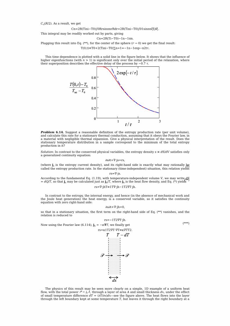
Cn(R/2).Asaresult,weget

Cn=2R(Tini−T0)∫0RrsinπnrRdr=2R(Tini−T0)∫01sinπnξξdξ.Thisintegralmaybereadilyworkedoutbyparts,giving

Cn=2R(Ti−T0)−1n−1πn.PluggingthisresultintoEq.(**),forthecenterofthesphere(r→0)wegetthefinalresult:

T(0,t)≡T0+2(Tini−T0)∑n=1∞−1n−1exp−n2tτ.

Thistimedependenceisplottedwithasolidlineinthefigurebelow.Itshowsthattheinfluenceofhighereigenfunctions(withn>1)issignificantonlyovertheinitialperiodoftherelaxation,wheretheirsuperpositiondescribestheeffectivedelayoftheprocessby∼0.7τ.

Problem 6.14. Suggest a reasonabledefinition of the entropyproduction rate (perunit volume),andcalculatethisrateforastationarythermalconduction,assumingthatitobeystheFourierlaw,inamaterialwithnegligiblethermalexpansion.Giveaphysicalinterpretationoftheresult.Doesthestationary temperature distribution in a sample correspond to the minimum of the total entropyproductioninit?

Solution:Incontrasttotheconservedphysicalvariables,theentropydensitys≡dS/dVsatisfiesonlyageneralizedcontinuityequation:

∂s∂t+∇⋅js=rs,(wherejs is theentropycurrentdensity),and itsright-handside isexactlywhatmayrationallybecalledtheentropyproductionrate.Inthestationary(time-independent)situation,thisrelationyields

rs=∇⋅js.AccordingtothefundamentalEq.(1.19),withtemperature-independentvolumeV,wemaywritedS=dQ/T,sothatjsmaybecalculatedjustasjh/T,wherejhistheheatflowdensity,andEq.(*)yields

rs=∇⋅jhT≡1T∇⋅jh−1T2∇T⋅jh.

Incontrasttotheentropy,theinternalenergy,andhence(intheabsenceofmechanicalworkandthe Joule heat generation) the heat energy, is a conserved variable, so it satisfies the continuityequationwithzeroright-handside:

∂u∂t+∇⋅jh=0,sothat inastationarysituation,thefirsttermontheright-handsideofEq.(**)vanishes,andtherelationisreducedto

rs=−1T2∇T⋅jh.NowusingtheFourierlaw(6.114),jh=−κ∇T,wefinallyget

rs=κ1T2∇T⋅∇T≡κ∇TT2.

Thephysicsofthisresultmaybeseenmoreclearlyonasimple,1Dexampleofauniformheat

flow,withthetotalpower ,throughalayerofareaAandsmallthicknessdx,undertheeffectofsmalltemperaturedifferencedT=(∂T/∂x)dx—seethefigureabove.TheheatflowsintothelayerthroughtheleftboundarykeptatsometemperatureT,butleavesitthroughtherightboundaryata

lowertemperature,T−dT,sothatthecorrespondingentropyflows, ,and ,arenotequal,evenif theheatpowerflows are.Therateof the totalentropyproduction in the layer isdeterminedbythedifferenceoftheseflows:

AfterpluggingtheFourierconductionlawforthis1Dsituation, ,fortheentropyproductionspecificrate,rs≡dRs/dV=dRs/(Adx),weobtain

i.e.thesameresultaswewouldgetforthissituationfromthemoregeneralEq.(***).NownotethataccordingtoEq.(6.119)ofthelecturenotes,

∂T∂t=DT∇2T,thestationarytemperaturedistributioninauniformsampleofvolumeVobeystheLaplaceequation∇2T = 0. However, it is well known44, that this equation is equivalent to the requirement of theminimumofthefollowingfunctional:

∫V∇T2d3r.Comparingthisexpressionwiththefullrateofentropyproductioninthesample,followingfromEq.(***),

Rs≡∫Vrsd3r=κ∫V∇TT2d3r,we see that if the temperature gradient is so low that T ≈ const, the stationary distribution oftemperaturecorrespondstotheminimumofRs.However,thiscomparisonalsoshowsthatthisso-calledminimumentropyproductionprinciple isnotexact.(Itmaybealsoviolatedbythesample’snon-uniformity.)

References[1]RösslerCetal2011NewJ.Phys.13113006[2]SchwabKetal2000Nature404974[3]ShokleyW1950ElectronsandHolesinSemiconductors(VanNostrand)[4]SmithD1995Thin-FilmDeposition(McGraw-Hill)[5]ZimanJ1979PrinciplesoftheTheoryofSolids2nded(CambridgeUniversityPress)[6]AshcroftNandMerminN1976SolidStatePhysics(W.B.Saunders)

1Formorediscussionofthisissuesee,e.g.PartEMsection6.4.2Anintroductiontothismethodmaybefound,forexample,inPartEMsection2.5.3AnotherpossiblecontributiontothefunctionXk(x),proportionaltosinkx,hasbeendroppedbecausethatfunctionevidentlyshouldretainitsinitialsymmetry:Xk(−x)=Xk(x).4See,e.g.Eq.(A.88).5TheWKBapproximation (discussed, e.g. inPartQM section2.4)maybeused to show that the result of this analysis is alsovalid for the so-called ‘adiabatic’channelswhosecross-section is slowlychangingalong the length.Moreover, strictly speaking the result isonly valid for suchadiabatic channels,with smoothedinterfacesbetweenthebulkconductorsandthechannel,becauseonlyforsuchgeometrytheelectronscatteringatthelinkentrance/exit(theeffectartfullysweptunderthecarpetintheprovidedsolution:-)isnegligible.6Theleftinequalityensuresthatthisstateinconductor2isempty,andhenceavailableforoccupationbythetravelingelectron.7See,e.g.PartQMEq.(1.100).8See,e.g.PartQMEq.(2.5)with∂φ/∂x=kx.9See,e.g.PartQMsection3.2.10See,e.g.[2]andreferencestherein.11AnothereffectistheCoulombinteractionoftheelectronswithinthegas,leading,inparticular,totheirscattering.Insolids,thiseffectistypicallylessimportant,duetothecompensatingpositivechargeoftheatomiclattice.Incontrast,thechargeQdiscussedinthisproblemistheuncompensatedchargeofadditionalelectrons.12Ifthisformulaisnotevident,thereadermayconsultPartEMsections2.2and3.4.13NotethatbothCeandCqarealwayspositive,regardlessofthechargeoftheparticles(e.g.electrons).14This fact emphasizes a broad similarity between the thermal activation of atomic/molecular condensation centers in usual gases, and of dopant atoms insemiconductors.15Noteagainthatniisaverystrongfunctionoftemperature—seethesecondofEqs.(6.60).16Note that in somesemiconductors thedegeneracyofelectronson the levelεAmaybedifferent from2. (InSi, it is equal to4.) In this case, the factor2 in theexpressionforn−,andhenceinEq.(**),shouldbereplacedwiththeproperdegeneracyfactor.However,thischangeofthepre-exponentialfactorhasvirtuallynoeffectontheresultspresentedbelow,inparticularontheplotsofμversusnD.17Foramoredetaileddiscussionofsemiconductordopingstatistics(aswellassomeotherissuesdiscussedinsection6.4),Icanrecommendtheclassicalmonograph[3].18Inchemistryandrelatedfields,thisprocessisfrequentlycalledeffusion.19BothinvolveddimensionlessintegralsareofthetypeEq.(A.36e),withn=2andn=1,respectively.20Notethatthesameresult(**)maybealsoobtainedinaslightlydifferentway(actually,usedinmosttextbooks),byconsideringwhatfractionfofparticles,inanelementaryvolumed3r=r2drdΩ,withr= andhencedr= ,hasvelocitiesdirectedtowardtheorifice(theanswerisf=Acosθ/4πr2),and then integrating theresultingparticlenumberdN=nfdr3overallvelocitiesinsphericalcoordinates,withd3 = .Letmeleavethecompletionofthisapproachforthereaderasasimple,butusefuladditionalexercise.21See,e.g.chapters6and7in[4].22See,e.g.PartCMEq.(8.56).Notethedifferencebetweentheshearviscositycoefficientηconsideredinthisproblem,andthedragcoefficientηwhosecalculationwasthetaskofproblem3.2.Despitethesimilartraditionalnotation,andbelongingtothesamerealm(kinematicfriction),thesecoefficientshavedifferentdefinitions,andevendifferentdimensionalities.23Thisassumptionisperhapsthelargestsourceofimprecisionofnumericalcoefficientsinourestimates.24Asthesolutionofthenextproblemwillshow,inmanycasesthisisnotaverygoodassumption,andmaycostusonemorenumericalfactoroftheorderof1.25Accordingtothedefinition(6.40)ofμ′,foragasofcharge-freeparticles,μ′=μ,sothesetwoconditionsareequivalent.26ComparingthisexpressionwithEq.(6.104)ofthelecturenotes,pleaserememberthatourcurrentcalculationisforμ=const,sothattheterms,proportionaltothechemicalpotentialonbothsidesoftheinterface,cancel.27Itsaccountwouldrequireaspecificationofthethermally-activatedinternaldegreesoffreedomoftheparticle.28Asareminder,accordingtotheequipartitiontheorem,forfreeclassicalparticleswithnegligiblethermalexcitationof their internaldegreesoffreedom,i.e.withthreehalf-degreesoffreedom,cV=3/2—seeEq.(3.31).29Notethatherethefactoringoftheaveragesismore‘clean’(lessapproximate)thanintheprevioustask,becausethetwoCartesiancomponentsofthevelocity, and

,areindependent.30Iamsorrytouseforthecross-sectionthesameletterasfortheelectricOhmicconductivity.(Bothnotationsareverytraditional.)Letmehopethiswouldnotleadtoconfusion,becausetheconductivityisnotdiscussedinthisproblem.31Thisdefinitioniscommonforparticlescatteringdescriptionisclassicalandquantummechanics,andmapsonasimilardefinitionatthewavescattering—see,e.g.

PartCM(3.70),PartEMEq.(8.39),andPartQMEq.(3.59).32Thisparameterisdefinedasthesmallestdistancebetweentheparticlecentersintheabsenceofscattering—see,e.g.PartCMsection3.5.33Asperhapsthemostimportantexample,attheso-calledRutherfordscatteringbyaCoulombpotentialU∝1/r,thefullcross-sectionσisinfinite,atleastinthelimitn→0—see,e.g.PartCMEq.(3.73).34See,e.g.either[5]or[6].35ThattableusestraditionalunitsmPa·s≡(10−3Nm−2)·s≡10−3kg(m·s)−1.36Foragasofchargedparticles,forexamplesofelectronsinametal,thiscondition,jn≡j/q=0,maybeimposedsimplybydisconnectingalongsample,madeofthismetal,fromanexternalconductingelectriccircuit—see,e.g.figure6.12ofthelecturenotes.37NotethatthisisessentiallyEq.(6.102),onlywithμ=μ′.38TheyarebothofthetypeEq.(A.34a),onewiths=7/2,andtheotheronewiths=5/2—seealsoEq.(A.34e).39ItisinstructivetocomparethisexpressionwithEq.(6.101)ofthelecturenotes,validintheopposite,degeneratelimitT≪μ.40Thecalculationmaybesimplifiedtakingintoaccountthatinthecasejn=0wearepursuing,wemayuseEq.(6.104)withoutthesecondtermintheparentheses—seetheremarkimmediatelyfollowingthatformula.41Notethatatitsderivationwehaveignoredtheparticleflow,sothatthecomparisonoftheresultingκwithκefismoreorlessfair—atleastwithintheframeworkofverycrudeassumptionsmadeatthederivation.42See,e.g.Eq.(A.67)with∂/∂θ=∂/∂φ=0.43Thisfactiswellknownfromelectrodynamicsandquantummechanics—see,e.g.eitherPartEMsection8.1,inparticular,Eqs.(8.7)–(8.8),orPartQMsection3.1,inparticularEqs.(3.4)–(3.7).44Foraproof,see,e.g.thesolutionofPartEMproblem1.16,withthereplacementϕ→T.

(A.1)

(A.2a)

(A.2b)

(A.3)

(A.4a)

(A.4b)

(A.5)

(A.6)

(A.7)

(A.8a)

(A.8b)

(A.9a)(A.9b)

(A.10a)

(A.10b)

(A.11a)

(A.11b)

IOPPublishing

StatisticalMechanicsProblemswithsolutionsKonstantinKLikharev

AppendixA

Selectedmathematicalformulas

Thisappendix listsselectedmathematical formulasthatareusedinthis lecturecourseseries,butnotalwaysrememberedbystudents(andsomeinstructors:-).

A.1ConstantsEuclideancircle’slength-to-diameterratio:

π=3.141592653…;π1/2≈1.77.Naturallogarithmbase:

e≡limn→∞1+1nn=2.718281828…;fromthatvalue,thelogarithmbaseconversionfactorsareasfollows(ξ>0):

lnξlog10ξ=ln10≈2.303,log10ξlnξ=1ln10≈0.434.TheEuler(or‘Euler–Mascheroni’)constant:

γ≡limn→∞1+12+13+…1n−lnn=0.5771566490…;eγ≈1.781.

A.2Combinatorics,sums,andseries(i)Combinatorics

Thenumberofdifferentpermutations,i.e.orderedsequencesofkelementsselectedfromasetofndistinctelements(n⩾k),is

Pkn≡n⋅(n−1)⋯(n−k+1)=n!(n−k)!;inparticular,thenumberofdifferentpermutationsofallelementsoftheset(n=k)is

Pkk=k⋅(k−1)⋯2⋅1=k!.Thenumberofdifferentcombinations,i.e.unorderedsequencesofkelementsfromasetofn⩾kdistinctelements,isequaltothebinomialcoefficient

Ckn≡nk≡PknPkk=n!k!(n−k)!.Inanalternative,verypopular ‘ball/boxlanguage’,nCk isthenumberofdifferentwaystoputinabox,inanarbitraryorder,kballsselectedfromndistinctballs.Ageneralizationofthebinomialcoefficientnotionisthemultinomialcoefficient,

Cnk1,k2,…kl≡n!k1!k2!…kl!,withn=∑j=1lkj,which,inthestandardmathematicallanguage,isanumberofdifferentpermutationsinamultisetof l distinctelement types fromann-elementsetwhichcontainskj(j=1, 2,…l)elements of each type. In the ‘ball/box language’, the coefficient (A.6) is the number ofdifferentwaystodistributendistinctballsbetweenldistinctboxes,eachtimekeepingthenumber (kj) of balls in the jth box fixed, but ignoring their order inside the box. ThebinomialcoefficientnCk(A.5)isaparticularcaseofthemultinomialcoefficient(A.6)forl=2-countingtheexplicitboxforthefirstone,andtheremainingspaceforthesecondbox,sothatifk1≡k,thenk2=n−k.One more important combinatorial quantity is the number Mn

(k) of ways to place nindistinguishableballsintokdistinctboxes.ItmaybereadilycalculatedfromEq.(A.5)asthenumberofdifferentwaystoselect(k−1)partitionsbetweentheboxesinanimaginedlinearrowof(k−1+n)‘objects’(ballsintheboxesandpartitionsbetweenthem):

Mn(k)=Ck−1n−1+k≡k−1+n!k−1!n!.(ii)Sumsandseries

Arithmeticprogression:r+2r+⋯+nr≡∑k=1nkr=n(r+nr)2;

inparticular,atr=1itisreducedtothesumofnfirstnaturalnumbers:1+2+⋯+n≡∑k=1nk=n(n+1)2.

Sumsofsquaresandcubesofnfirstnaturalnumbers:12+22+⋯+n2≡∑k=1nk2=n(n+1)(2n+1)6;

13+23+⋯+n3≡∑k=1nk3=n2(n+1)24.TheRiemannzetafunction:

ζ(s)≡1+12s+13s+⋯≡∑k=1∞1ks;theparticularvaluesfrequentlymetinapplicationsare

ζ32≈2.612,ζ2=π26,ζ52≈1.341,ζ3≈1.202,ζ(4)=π490,ζ5≈1.037.Finitegeometricprogression(forrealλ≠1):

1+λ+λ2+⋯+λn−1≡∑k=0n−1λk=1−λn1−λ;inparticular, ifλ2<1, theprogressionhasa finite limitatn→∞ (called thegeometricseries):

(A.12)

(A.13)

(A.14a)

(A.14b)

(A.15a)

(A.15b)

(A.16a)(A.16b)

(A.17a)(A.17b)(A.17c)

(A.18a)(A.18b)(A.18c)

(A.18d)

(A.19)

(A.20)

(A.21)

(A.22)

(A.23)

(A.24)

(A.25)

(A.26)

(A.27)

(A.28)(A.29a)(A.29b)

(A.30a)(A.30b)(A.30c)(A.30d)

(A.31a)(A.31b)

limn→∞∑k=0n−1λk=∑k=0∞λk=11−λ.Binomialsum(orthe‘binomialtheorem’):

1+an=∑k=0nCknak,wherenCkarethebinomialcoefficientsdefinedbyEq.(A.5).TheStirlingformula:

limn→∞lnn!=n(lnn−1)+12ln(2πn)+112n−1360n3+…;formostapplicationsinphysics,thefirstterm1issufficient.TheTaylor(or‘Taylor–Maclaurin’)series:foranyinfinitelydifferentiablefunctionf(ξ):

limξ˜→0f(ξ+ξ˜)=f(ξ)+dfdξ(ξ)ξ˜+12!d2fdξ2(ξ)ξ˜2+⋯=∑k=0∞1k!dkfdξk(ξ)ξ˜k;notethat formanyfunctionsthisseriesconvergesonlywithina limited,sometimessmallrangeofdeviationsξ˜.Forafunctionofseveralarguments,f(ξ1,ξ2,…,ξN),thefirsttermsoftheTaylorseriesare

limξ˜k→0f(ξ1+ξ˜1,ξ2+ξ˜2,⋯)=fξ1,ξ2,⋯+∑k=1N∂f∂ξkξ1,ξ2,⋯ξ˜k+12!∑k,k′=1N∂2f∂kξ∂ξk′ξ˜kξ˜k′+⋯TheEuler–Maclaurinformula,validforanyinfinitelydifferentiablefunctionf(ξ):

∑k=1nf(k)=∫0nf(ξ)dξ+12f(n)−f(0)+16⋅12!dfdξ(n)−dfdξ(0)−130⋅14!d3fdξ3(n)−d3fdξ3(0)+142⋅16!d5fdξ5(n)−d5fdξ5(0)+⋯;thecoefficientsparticipatinginthisformulaaretheso-calledBernoullinumbers2:

B1=12,B2=16,B3=0,B4=130,B5=0,B6=142,B7=0,B8=130,⋯

A.3BasictrigonometricfunctionsTrigonometricfunctionsofthesumandthedifferenceoftwoarguments3:

cosa±b=cosacosb∓sinasinb,sina±b=sinacosb±cosasinb.Sumsoftwofunctionsofarbitraryarguments:

cosa+cosb=2cosa+b2cosb−a2,cosa−cosb=2sina+b2sinb−a2,sina±sinb=2sina±b2cos±b−a2.Trigonometricfunctionproducts:

2cosacosb=cos(a+b)+cos(a−b),2sinacosb=sin(a+b)+sin(a−b),2sinasinb=cos(a−b)−cos(a+b);fortheparticularcaseofequalarguments,b=a,thesethreeformulasyieldthefollowingexpressionsforthesquaresoftrigonometricfunctions,andtheirproduct:

cos2a=121+cos2a,sinacosa=12sin2a,sin2a=121−cos2a.Cubesoftrigonometricfunctions:

cos3a=34cosa+14cos3a,sin3a=34sina−14sin3a.Trigonometricfunctionsofacomplexargument:

sin(a+ib)=sinacoshb+icosasinhb,cos(a+ib)=cosacoshb−isinasinhb.Sumsoftrigonometricfunctionsofnequidistantarguments:

∑k=1nsincoskξ=sincosn+12ξsinn2ξ/sinξ2.

A.4GeneraldifferentiationFulldifferentialofaproductoftwofunctions:

d(fg)=(df)g+f(dg).Fulldifferentialofafunctionofseveralindependentarguments,f(ξ1,ξ2,…,ξn):

df=∑k=1n∂f∂ξkdξk.CurvatureoftheCartesianplotofa1Dfunctionf(ξ):

κ≡1R=d2f/dξ21+df/dξ23/2.

A.5GeneralintegrationIntegrationbyparts-immediatelyfollowsfromEq.(A.22):

∫g(A)g(B)fdg=fgBA−∫f(A)f(B)gdf.Numerical(approximate)integrationof1Dfunctions:thesimplesttrapezoidalrule,

∫abf(ξ)dξ≈hfa+h2+fa+3h2+⋯+fb−h2=h∑n=1Nfa−h2+nh,h≡b−aN.has relatively low accuracy (error of the order of (h3/12)d2f/dξ2 per step), so that thefollowingSimpsonformula,

∫abf(ξ)dξ≈h3f(a)+4f(a+h)+2f(a+2h)+⋯+4f(b−h)+f(b),h≡b−a2N,whoseerrorperstepscalesas(h5/180)d4f/dξ4,isusedmuchmorefrequently4.

A.6Afew1Dintegrals5(i)Indefiniteintegrals:

Integralswith(1+ξ2)1/2:∫1+ξ21/2dξ=ξ21+ξ21/2+12ln∣ξ+(1+ξ2)1/2∣,

∫dξ1+ξ21/2=ln∣ξ+1+ξ21/2∣,∫dξ1+ξ23/2=ξ1+ξ21/2.Miscellaneousindefiniteintegrals:

∫dξξ(ξ2+2aξ−1)1/2=arccosaξ−1∣ξ∣a2+11/2,∫sinξ−ξcosξ2ξ5dξ=2ξsin2ξ+cos2ξ−2ξ2−18ξ4,∫dξa+bcosξ=2a2−b21/2tan−1a−ba2−b21/2tanξ2,fora2>b2.∫dξ1+ξ2=tan−1ξ.

(ii)Semi-definiteintegrals:Integralswith1/(eξ±1):

∫a∞dξeξ+1=ln1+e−a,

(A.32a)(A.32b)

(A.32c)

(A.33a)(A.33b)

(A.34a)

(A.34b)

(A.34c)

(A.34d)

(A.34e)

(A.35a)(A.35b)

(A.35c)(A.35d)

(A.35e)

(A.36a)

(A.36b)(A.36c)

(A.36d)

(A.36e)

(A.37)(A.38)(A.39)

(A.40)(A.41)

(A.42a)(A.42b)

(A.43)

(A.44)

(A.45)

(A.46)

(A.47)

(A.48)

(A.49a)

(A.49b)

∫a>0∞dξeξ−1=ln11−e−a.(iii)Definiteintegrals:

Integralswith1/(1+ξ2):6∫0∞dξ1+ξ2=π2,

∫0∞dξ1+ξ23/2=1;moregenerally,

∫0∞dξ1+ξ2n=π22n−3!!2n−2!!≡π21⋅3⋅5…2n−32⋅4⋅6…2n−2,forn=2,3,…Integralswith(1−ξ2n)1/2:

∫01dξ1−ξ2n1/2=π1/22nΓ12n/Γn+12n,∫011−ξ2n1/2dξ=π1/24nΓ12n/Γ3n+12n,where Γ(s) is the gamma-function, which is most often defined (for Re s > 0) by thefollowingintegral:

∫0∞ξs−1e−ξdξ=Γ(s).Thekeypropertyofthisfunctionistherecurrencerelation,validforanys≠0,−1,−2,…:

Γ(s+1)=sΓ(s).Since,accordingtoEq. (A.34a),Γ(1)=1,Eq.(A.34b) fornon-negative integers takes theform

Γ(n+1)=n!,forn=0,1,2,⋯(where0!≡1).Becauseofthis,forintegers=n+1⩾1,Eq.(A.34a)isreducedto

∫0∞ξne−ξdξ=n!.Other frequently met values of the gamma-function are those for positive semi-integerarguments:

Γ12=π1/2,Γ32=12π1/2,Γ52=12⋅32π1/2,Γ72=12⋅32⋅52π1/2,….Integralswith1/(eξ±1):

∫0∞ξs−1dξeξ+1=(1−21−s)Γ(s)ζ(s),fors>0,∫0∞ξs−1dξeξ−1=Γ(s)ζ(s),fors>1,whereζ(s)istheRiemannzeta-function—seeEq.(A.10).Particularcases:fors=2n,

∫0∞ξ2n−1dξeξ+1=22n−1−12nπ2nB2n,∫0∞ξ2n−1dξeξ−1=(2π)2n4nB2n.whereBnaretheBernoullinumbers—seeEq. (A.15).Fortheparticularcases=1 (whenEq.(A.35a)yieldsuncertainty),

∫0∞dξeξ+1=ln2.Integralswithexp{−ξ2}:

∫0∞ξse−ξ2dξ=12Γs+12,fors>−1;forapplicationsthemostimportantparticularvaluesofsare0and2:

∫0∞e−ξ2dξ=12Γ12=π1/22,∫0∞ξ2e−ξ2dξ=12Γ32=π1/24,althoughwewillalsorunintothecasess=4ands=6:

∫0∞ξ4e−ξ2dξ=12Γ52=3π1/28,∫0∞ξ6e−ξ2dξ=12Γ72=15π1/216;foroddintegervaluess=2n+1(withn=0,1,2,…),Eq.(A.36a)takesasimplerform:

∫0∞ξ2n+1e−ξ2dξ=12Γn+1=n!2.Integralswithcosineandsinefunctions:

∫0∞cosξ2dξ=∫0∞sinξ2dξ=π81/2.∫0∞cosξa2+ξ2dξ=π2ae−a.∫0∞sinξξ2dξ=π2.Integralswithlogarithms:

∫01lna+1−ξ21/2a−1−ξ21/2dξ=πa−a2−11/2,fora⩾1.∫01ln1+1−ξ1/2ξ1/2dξ=1.IntegralrepresentationsoftheBesselfunctionsofintegerorder:

Jn(α)=12π∫−π+πei(αsinξ−nξ)dξ,sothateiαsinξ=∑k=−∞∞Jk(α)eikξ;In(α)=1π∫0πeαcosξcosnξdξ.

A.73Dvectorproducts(i)Definitions:

Scalar(‘dot-’)product:a⋅b=∑j=13ajbj,

whereajandbjarevectorcomponentsinanyorthogonalcoordinatesystem.Inparticular,thevectorsquared(thesameasthenormsquared):

a2≡a⋅a=∑j=13aj2≡∥a∥2.Vector(‘cross-’)product:

a×b≡n1(a2b3−a3b2)+n2(a3b1−a1b3)+n3(a1b2−a2b1)=n1n2n3a1a2a3b1b2b3,where {nj} is the set of mutually perpendicular unit vectors7 along the correspondingcoordinatesystemaxes8.Inparticular,Eq.(A.45)yields

a×a=0.(ii)Corollaries(readilyverifiedbyCartesiancomponents):

Doublevectorproduct(theso-calledbacminuscabrule):a×(b×c)=b(a⋅c)−c(a⋅b).

Mixedscalar–vectorproduct(theoperandrotationrule):a⋅b×c=b⋅c×a=c⋅a×b.

Scalarproductofvectorproducts:a×b⋅c×d=a⋅cb⋅d−a⋅db⋅c;

intheparticularcaseof twosimilaroperands(say,a=candb=d), the last formula isreducedto

a×b2=(ab)2−(a⋅b)2.

(A.50)

(A.51)

(A.52)

(A.53)

(A.54)

(A.55)

(A.56)

(A.57)

(A.58)

(A.60)

(A.61)

(A.62)

(A.63)

(A.64)

(A.66)

(A.67)

(A.68)

(A.69)

A.8Differentiationin3DCartesiancoordinatesDefinitionofthedel(or‘nabla’)vector-operator∇:9

∇≡∑j=13nj∂∂rj,where rj is a set of linear and orthogonal (Cartesian) coordinates along directionsnj. Inaccordancewiththisdefinition,theoperator∇actingonascalar functionofcoordinates,f(r),10givesitsgradient,i.e.anewvector:

∇f≡∑j=13nj∂f∂rj≡gradf.Thescalarproductofdelbyavectorfunctionofcoordinates(avectorfield),

f(r)≡∑j=13njfj(r),compiled formally followingEq. (A.43), is a scalar function—thedivergence of the initialfunction:

∇⋅f≡∑j=13∂fj∂rj≡divf,whilethevectorproductof∇andf,formedinaformalaccordancewithEq.(A.45),isanewvector-thecurl(inEuropeantradition,calledrotoranddenotedrot)off:

∇×f≡n1n2n3∂∂r1∂∂r2∂∂r3f1f2f3=n1∂f3∂r2−∂f2∂r3+n2∂f1∂r3−∂f3∂r1+n3∂f2∂r1−∂f1∂r2≡curlf.One more frequently met ‘product’ is (f·∇)g, where f and g are two arbitrary vectorfunctionsofr.ThisproductshouldbealsounderstoodinthesenseimpliedbyEq.(A.43),i.e.asavectorwhosejthCartesiancomponentis

f⋅∇gj=∑j′=13fj′∂gj∂rj′.

A.9TheLaplaceoperator∇2≡∇·∇ExpressioninCartesiancoordinates—intheformalaccordancewithEq.(A.44):

∇2=∑j=13∂2∂rj2.Accordingtoitsdefinition,theLaplaceoperatoractingonascalarfunctionofcoordinatesgivesanewscalarfunction:

∇2f≡∇⋅∇f=divgradf=∑j=13∂2f∂rj2.On the other hand, acting on a vector function (A.52), the operator ∇2 returns anothervector:

∇2f=∑j=13nj∇2fj.Note that Eqs. (A.56)–(A.58) are only valid in Cartesian (i.e. orthogonal and linear)coordinates,butgenerallynotinother(evenorthogonal)coordinates—see,e.g.Eqs.(A.61),(A.64),(A.67)and(A.70)below.

A.10Operators∇and∇2inthemostimportantsystemsoforthogonalcoordinates11

(i)Cylindrical12coordinates{ρ,φ,z}(seefigurebelow)maybedefinedbytheirrelationswiththeCartesiancoordinates:

Gradientofascalarfunction:∇f=nρ∂f∂ρ+nφ1ρ∂f∂φ+nz∂f∂z.

TheLaplaceoperatorofascalarfunction:∇2f=1ρ∂∂ρρ∂f∂ρ+1ρ2∂2f∂φ2+∂2f∂z2,

Divergenceofavectorfunctionofcoordinates(f=nρfρ+nφfφ+nzfz):∇⋅f=1ρ∂ρfρ∂ρ+1ρ∂fφ∂φ+∂fz∂z.

Curlofavectorfunction:∇×f=nρ1ρ∂fz∂φ−∂fφ∂z+nφ∂fρ∂z−∂fz∂ρ+nz1ρ∂(ρfφ)∂ρ−∂fρ∂φ.

TheLaplaceoperatorofavectorfunction:∇2f=nρ∇2fρ−1ρ2fρ−2ρ2∂fφ∂φ+nφ∇2fφ−1ρ2fφ+2ρ2∂fρ∂φ+nz∇2fz.

(ii)Sphericalcoordinates{r,θ,φ}(seefigurebelow)maybedefinedas:

Gradientofascalarfunction:∇f=nr∂f∂r+nθ1r∂f∂θ+nφ1rsinθ∂f∂φ.

TheLaplaceoperatorofascalarfunction:∇2f=1r2∂∂rr2∂f∂r+1r2sinθ∂∂θsinθ∂f∂θ+1(rsinθ)2∂2f∂φ2.

Divergenceofavectorfunctionf=nrfr+nθfθ+nφfφ:∇⋅f=1r2∂r2fr∂r+1rsinθ∂(fθsinθ)∂θ+1rsinθ∂fφ∂φ.

Curlofasimilarvectorfunction:

(A.70)

(A.71)

(A.72)

(A.73)

(A.74a)

(A.74b)

(A.75)(A.76)(A.77)

(A.78)

(A.79)

(A.80)

(A.81)

(A.82)

(A.83)

(A.84a)

(A.84b)

(A.85)

(A.86)

(A.87a)

(A.87b)

(A.88)

(A.89)

(A.90)

∇×f=nr1rsinθ∂(fφsinθ)∂θ−∂fθ∂φ+nθ1r1sinθ∂fr∂φ−∂(rfφ)∂r+nφ1r∂(rfθ)∂r−∂fr∂θ.TheLaplaceoperatorofavectorfunction:

∇2f=nr∇2fr−2r2fr−2r2sinθ∂∂θ(fθsinθ)−2r2sinθ∂fφ∂φ+nθ∇2fθ−1r2sin2θfθ+2r2∂fr∂θ−2cosθr2sin2θ∂fφ∂φ+nφ∇2fφ−1r2sin2θfφ+2r2sinθ∂fr∂φ+2cosθr2sin2θ∂fθ∂φ.

A.11Productsinvolving∇(i)Usefulzeros:

Foranyscalarfunctionf(r),∇×∇f≡curlgradf=0.

Foranyvectorfunctionf(r),∇⋅∇×f≡divcurlf=0.

(ii)TheLaplaceoperatorexpressedviathecurlofacurl:∇2f=∇∇⋅f−∇×∇×f.

(iii)Spatialdifferentiationofaproductofascalarfunctionbyavectorfunction:Thescalar3DgeneralizationofEq.(A.22)is

∇⋅fg=∇f⋅g+f∇⋅g.Itsvectorgeneralizationissimilar:

∇×fg=∇f×g+f∇×g.

(iv)Spatialdifferentiationofproductsoftwovectorfunctions:∇×f×g=f∇⋅g−f⋅∇g−∇⋅fg+g⋅∇f,

∇f⋅g=f⋅∇g+g⋅∇f+f×∇×g+g×∇×f,∇⋅f×g=g⋅∇×f−f⋅∇×g.

A.12Integro-differentialrelations(i)ForanarbitrarysurfaceSlimitedbyclosedcontourC:

TheStokestheorem,validforanydifferentiablevectorfieldf(r):∫S∇×f⋅d2r≡∫S∇×fnd2r=∮Cf⋅dr≡∮Cfτdr,

whered2r ≡nd2r is the elementary area vector (normal to the surface), and dr is theelementarycontourlengthvector(tangentialtothecontourline).

(ii)ForanarbitraryvolumeVlimitedbyclosedsurfaceS:Divergence(or‘Gauss’)theorem,validforanydifferentiablevectorfieldf(r):

∫V∇⋅fd3r=∮Sf⋅d2r≡∮Sfnd2r.Green’stheorem,validfortwodifferentiablescalarfunctionsf(r)andg(r):

∫Vf∇2g−g∇2fd3r=∮Sf∇g−g∇fnd2r.Anidentityvalidforanytwoscalarfunctionsfandg,andavectorfieldjwith∇·j=0(alldifferentiable):

∫Vf(j⋅∇g)+g(j⋅∇f)d3r=∮Sfgjnd2r.

A.13TheKroneckerdeltaandLevi-Civitapermutationsymbols

TheKroneckerdeltasymbol(definedforintegerindices):δjj′≡1,ifj′=j,0,otherwise.

TheLevi-Civitapermutationsymbol(mostfrequentlyusedfor3integerindices,eachtakingoneofvalues1,2,or3):

εjj′j″≡+1,iftheindicesfollowinthe‘correct’(‘even’)order:1→2→3→1→2…,−1,iftheindicesfollowinthe‘incorrect’(‘odd’)order:1→3→2→1→3…,0,ifanytwoindicescoincide.RelationbetweentheLevi-CivitaandtheKroneckerdeltaproducts:

εjj′j″εkk′k″=∑l,l′,l″=13δjlδjl′δjl″δj′lδj′l′δj′l″δj″lδj″l′δj″l″;summationofthisrelation,writtenfor3differentvaluesofj=k,overthesevaluesyieldstheso-calledcontractedepsilonidentity:

∑j=13εjj′j″εjk′k″=δj′k′δj″k″−δj′k″δj″k′.

A.14Dirac’sdelta-function,signfunction,andtheta-functionDefinitionof1Ddelta-function(forreala<b):

∫abf(ξ)δ(ξ)dξ=f(0),ifa<0<b,0,otherwise,wheref(ξ)isanyfunctioncontinuousnearξ=0.Inparticular(iff(ξ)=1nearξ=0),thedefinitionyields

∫abδ(ξ)dξ=1,ifa<0<b,0,otherwise.Relationtothetheta-functionθ(ξ)andsignfunctionsgn(ξ)

δ(ξ)=ddξθ(ζ)=12ddξsgn(ξ),where

θ(ξ)≡sgn(ξ)+12=0,ifξ<0,1,ifξ>1,sgn(ξ)≡ξ∣ξ∣=−1,ifξ<0,+1,ifξ>1.Animportantintegral13:

∫−∞+∞eisξds=2πδ(ξ).3D generalization of the delta-function of the radius-vector (the 2D generalization issimilar):

∫Vfrδrd3r=f(0),if0∈V,0,otherwise;itmayberepresentedasaproductof1Ddelta-functionsofCartesiancoordinates:

δ(r)=δ(r1)δ(r2)δ(r3).

A.15TheCauchytheoremandintegralLet a complex function be analyticwithin a part of the complex plane , that is limitedby aclosedcontourCandincludespoint .Then

ThefirstoftheserelationsisusuallycalledtheCauchyintegraltheorem(orthe‘Cauchy–Goursat

theorem’),andthesecondone—theCauchyintegral(orthe‘Cauchyintegralformula’).

A.16Literature(i) Properties of some special functions are briefly discussed at the relevant points of thelecturenotes;inthealphabeticalorder:Airyfunctions:PartQMsection2.4;Besselfunctions:PartEMsection2.7;Fresnelintegrals:PartEMsection8.6;Hermitepolynomials:PartQMsection2.9;Laguerrepolynomials(bothsimpleandassociated):PartQMsection3.7;Legendrepolynomials,associatedLegendre functions:PartEM section2.8, andPartQMsection3.6;Sphericalharmonics:PartQMsection3.6;SphericalBesselfunctions:PartQMsections3.6and3.8.

(ii)Formoreformulas,andtheirdiscussion,Icanrecommendthefollowinghandbooks14:

HandbookofMathematicalFormulas[2];TablesofIntegrals,Series,andProducts[3];MathematicalHandbookforScientistsandEngineers[4];IntegralsandSeriesvolumes1and2[5];ApopulartextbookMathematicalMethodsforPhysicists[6]maybealsousedasaformulamanual.

Many formulas are also available from the symbolic calculation modules of thecommerciallyavailablesoftwarepackageslistedinsection(iv)below.

(iii)ProbablythemostpopularcollectionofnumericalcalculationcodesarethetwinmanualsbyWPressetal[1]:NumericalRecipesinFortran77;NumericalRecipes[inC++—KKL].

My lecture notes include very brief introductions to numerical methods of differentialequationsolution:ordinarydifferentialequations:PartCM,section5.7;partialdifferentialequations:PartCMsection8.5andPartEMsection2.11,whichincludereferencestoliteratureforfurtherreading.

(iv) The following are the most popular software packages for numerical and symboliccalculations,allwithplottingcapabilities(inthealphabeticalorder):Maple(www.maplesoft.com/products/maple/);MathCAD(www.ptc.com/engineering-math-software/mathcad/);Mathematica(www.wolfram.com/mathematica/);MATLAB(www.mathworks.com/products/matlab.html).

References[1]PressWetal1992NumericalRecipesinFortran772ndedn(Cambridge:CambridgeUniversityPress)

PressWetal2007NumericalRecipes3rdedn(Cambridge:CambridgeUniversityPress)[2]AbramowitzMandStegunI(eds)1965HandbookofMathematicalFormulas(NewYork:Dover),andnumerouslaterprintings.

Anupdatedversionofthiscollectionisnowavailableonlineathttp://dlmf.nist.gov/.[3]GradshteynIandRyzhikI1980TablesofIntegrals,Series,andProducts5thedn(NewYork:Academic)[4]KornGandKornT2000MathematicalHandbookforScientistsandEngineers2ndedn(NewYork:Academic)[5]PrudnikovAetal1986IntegralsandSeriesvol1(BocaRaton,FL:CRCPress)

PrudnikovAetal1986IntegralsandSeriesvol2(BocaRaton,FL:CRCPress)[6]ArfkenGetal2012MathematicalMethodsforPhysicists7thedn(NewYork:Academic)[7]DwightH1961TablesofIntegralsandOtherMathematicalFormulas4thedn(London:Macmillan)

1Actually,thisleadingtermwasderivedbyAdeMoivrein1733,beforeJStirling’swork.2NotethatdefinitionsofBk(orrathertheirsignsandindices)varyevenamongthemostpopularhandbooks.3Iamconfidentthatthereaderisquitecapableofderivingtherelations(A.16)byrepresentingtheexponentintheelementaryrelationei(a±b)=eiae±ibasasumofitsreal and imaginary parts, Eqs. (A.18) directly from Eqs. (A.16), and Eqs. (A.17) from Eqs. (A.18) by variable replacement; however, I am still providing theseformulastosavehisorhertime.(Quiteafewformulasbelowareincludedbecauseofthesamereason.)4Higher-orderformulas(e.g.theBoderule),andotherguidanceincludingready-for-usecodesforcomputercalculationsmaybefound,forexample,inthepopularreferencetextsbyWHPressetal[1].Inaddition,someadvancedcodesareusedassubroutinesinthesoftwarepackageslistedinthesamesection.Insomecases,theEuler–Maclaurinformula(A.15)mayalsobeusefulfornumericalintegration.5Apowerful(andfree)interactiveonlinetoolforworkingoutindefinite1Dintegralsisavailableathttp://integrals.wolfram.com/index.jsp.6Eq.(A.32a)followsimmediatelyfromEq.(A.30d),andEq.(A.32b)fromEq.(A.29b)—acouplemoreexamplesofthe(intentional)redundancyinthislist.7Otherpopularnotationsforthisvectorsetare{ej}and{rˆj}.8It is easy to use Eq. (A.45) to check that the direction of the product vector corresponds to the well-known ‘right-hand rule’ and to the even more convenientcorkscrewrule:ifwerotateacorkscrew’shandlefromthefirstoperandtowardthesecondone,itsaxismovesinthedirectionoftheproduct.9Onecanrunintothefollowingnotation:∇≡∂/∂r,whichisconvenientissomecases,butmaybemisleadinginquiteafewothers,soitwillbenotusedinthesenotes.10Inthis,andfournextsections,allscalarandvectorfunctionsareassumedtobedifferentiable.11SomeotherorthogonalcurvilinearcoordinatesystemsarediscussedinPartEM,section2.3.12Inthe2Dgeometrywithfixedcoordinatez,thesecoordinatesarecalledpolar.13Thecoefficientinthisrelationmaybereadilyrecalledbyconsideringitsleft-handpartastheFourier-integralrepresentationoffunctionf(s)≡1,andapplyingEq.(A.85)tothereciprocalFouriertransform

f(s)≡1=12π∫−∞+∞e−isξ[2πδ(ξ)]dξ.

14Onapersonalnote,perhaps90%ofallformulaneedsthroughoutmyresearchcareerweresatisfiedbyatiny,wonderfullycompiledoldbook[7],usedcopiesofwhich,ratheramazingly,arestillavailableontheWeb.

IOPPublishing

StatisticalMechanicsProblemswithsolutionsKonstantinKLikharev

AppendixB

Selectedphysicalconstants

Thelistednumericalvaluesoftheconstantsarefromthemostrecent(2014)InternationalCODATArecommendation(see,e.g.http://physics.nist.gov/cuu/Constants/index.html),besidesanewerresultforkB—see[1].Pleasenotetherecentlyannounced(but,bythisvolume’spresstime,notyetofficial)adjustment of the SI values - see, e.g. https://www.nist.gov/si-redefinition/meet-constants. Inparticular, thePlanckconstantwill alsogetadefinite value (within the interval specified in tableB.1),enablinganew,fundamentalstandardofthekilogram.

TableB.1.

Symbol Quantity SIvalueandunit Gaussianvalueandunit Relativermsuncertaintyc speedoflightin

freespace2.99792458×108ms−1

2.99792458×1010cms−1

0(definedvalue)

G gravitationconstant

6.6741×10−11m3

kg−1s−26.6741×10−8cm3g−1s−2

∼5×10−5

ℏ Planckconstant 1.05457180×10−34Js

1.05457180×10−27ergs

∼2×10−8

e elementaryelectriccharge

1.6021762×10−19C

4.803203×10−10statcoulomb

∼6×10−9

me electron’srestmass

0.91093835×10−30kg

0.91093835×10−27g

∼1×10−8

mp proton’srestmass 1.67262190×10−27kg

1.67262190×10−24g

∼1×10−8

μ0 magneticconstant 4π×10−7NA−2 – 0(definedvalue)

ε0 electricconstant 8.854187817×10−12Fm−1

– 0(definedvalue)

kB Boltzmannconstant

1.380649×10−23JK−1

1.3806490×10−16ergK−1

∼2×10−6

Comments:1. Thefixedvalueofcwasdefinedbyaninternationalconventionin1983,inordertoextendthe

official definition of the second (as ‘the duration of 9 192 631 770 periods of the radiationcorresponding to the transitionbetween the twohyperfine levelsof thegroundstateof thecesium-133 atom’) to that of the meter. The values are back-compatible with the legacydefinitionsof themeter (initially,as1/40000000thof theEarth’smeridian length)and thesecond (for a long time, as 1/(24× 60× 60)= 1/86 400th of the Earth’s rotation period),withintheexperimentalerrorsofthosemeasures.

2. ε0andμ0arenotreallythefundamentalconstants;intheSIsystemofunitsoneofthem(say,μ0)isselectedarbitrarily1,whiletheotheroneisdefinedviatherelationε0μ0=1/c2.

3. TheBoltzmannconstantkB isalsonotquite fundamental,because itsonly role is tocomplywiththeindependentdefinitionofthekelvin(K),asthetemperatureunitinwhichthetriplepointofwaterisexactly273.16K.IftemperatureisexpressedinenergyunitskBT(asisdone,forexample,inPartSMofthisseries),thisconstantdisappearsaltogether.

4. Thedimensionless finestructure (‘Sommerfeld’s’)constantα isnumerically the same inanysystemofunits:

α≡e2/4πε0ℏcinSIunitse2/ℏcinGaussianunits≈7.297352566×10−3≈1137.03599914,andisknownwithamuchsmallerrelativermsuncertainty(currently,∼3×10−10)thanthoseofthecomponentconstants.

References[1]GaiserCetal2017Metrologia54280[2]NewellD2014Phys.Today6735–41

1Notethattheselectedvalueofμ0maybechanged(abit)inafewyears—see,e.g.,[2].

IOPPublishing

StatisticalMechanicsProblemswithsolutionsKonstantinKLikharev

Bibliography

This section presents a partial list of textbooks and monographs used in the work on the EAPseries1,2.

PartCM:ClassicalMechanicsFetterALandWaleckaJD2003TheoreticalMechanicsofParticlesandContinua(NewYork:Dover)GoldsteinH,PooleCandSafkoJ2002ClassicalMechanics3rdedn(Reading,MA:AddisonWesley)GrangerRA1995FluidMechanics(NewYork:Dover)JoséJVandSaletanEJ1998ClassicalDynamics(Cambridge:CambridgeUniversityPress)LandauLDandLifshitzEM1976Mechanics3rdedn(Oxford:Butterworth-Heinemann)LandauLDandLifshitzEM1986TheoryofElasticity(Oxford:Butterworth-Heinemann)LandauLDandLifshitzEM1987FluidMechanics2ndedn(Oxford:Butterworth-Heinemann)SchusterHG1995DeterministicChaos3rdedn(NewYork:Wiley)SommerfeldA1964Mechanics(NewYork:Academic)SommerfeldA1964MechanicsofDeformableBodies(NewYork:Academic)

PartEM:ClassicalElectrodynamicsBatyginVVandToptyginIN1978ProblemsinElectrodynamics2ndedn(NewYork:Academic)GriffithsDJ2007IntroductiontoElectrodynamics3rdedn(EnglewoodCliffs,NJ:Prentice-Hall)JacksonJD1999ClassicalElectrodynamics3rdedn(NewYork:Wiley)LandauLDandLifshitzEM1984ElectrodynamicsofContinuousMedia2ndedn(Auckland:Reed)LandauLDandLifshitzEM1975TheClassicalTheoryofFields4thedn(Oxford:Pergamon)PanofskyWKHandPhillipsM1990ClassicalElectricityandMagnetism2ndedn(NewYork:Dover)StrattonJA2007ElectromagneticTheory(NewYork:Wiley)TammIE1979FundamentalsoftheTheoryofElectricity(Paris:Mir)ZangwillA2013ModernElectrodynamics(Cambridge:CambridgeUniversityPress)

PartQM:QuantumMechanicsAbersES2004QuantumMechanics(London:Pearson)AulettaG,FortunatoMandParisiG2009QuantumMechanics(Cambridge:CambridgeUniversityPress)CapriAZ2002NonrelativisticQuantumMechanics3rdedn(Singapore:WorldScientific)Cohen-TannoudjiC,DiuBandLaloëF2005QuantumMechanics(NewYork:Wiley)ConstantinescuF,MagyariEandSpiersJA1971ProblemsinQuantumMechanics(Amsterdam:Elsevier)GalitskiVetal2013ExploringQuantumMechanics(Oxford:OxfordUniversityPress)GottfriedKandYanT-M2004QuantumMechanics:Fundamentals2ndedn(Berlin:Springer)GriffithD2005QuantumMechanics2ndedn(EnglewoodCliffs,NJ:PrenticeHall)LandauLDandLifshitzEM1977QuantumMechanics(NonrelativisticTheory)3rdedn(Oxford:Pergamon)MessiahA1999QuantumMechanics(NewYork:Dover)MerzbacherE1998QuantumMechanics3rdedn(NewYork:Wiley)MillerDAB2008QuantumMechanicsforScientistsandEngineers(Cambridge:CambridgeUniversityPress)SakuraiJJ1994ModernQuantumMechanics(Reading,MA:Addison-Wesley)SchiffLI1968QuantumMechanics3rdedn(NewYork:McGraw-Hill)ShankarR1980PrinciplesofQuantumMechanics2ndedn(Berlin:Springer)SchwablF2002QuantumMechanics3rdedn(Berlin:Springer)

PartSM:StatisticalMechanicsFeynmanRP1998StatisticalMechanics2ndedn(Boulder,CO:Westview)HuangK1987StatisticalMechanics2ndedn(NewYork:Wiley)KuboR1965StatisticalMechanics(Amsterdam:Elsevier)LandauLDandLifshitzEM1980StatisticalPhysics,Part13rdedn(Oxford:Pergamon)LifshitzEMandPitaevskiiLP1981PhysicalKinetics(Oxford:Pergamon)PathriaRKandBealePD2011StatisticalMechanics3rdedn(Amsterdam:Elsevier)PierceJR1980AnIntroductiontoInformationTheory2ndedn(NewYork:Dover)PlishkeMandBergersenB2006EquilibriumStatisticalPhysics3rdedn(Singapore:WorldScientific)SchwablF2000StatisticalMechanics(Berlin:Springer)YeomansJM1992StatisticalMechanicsofPhaseTransitions(Oxford:OxfordUniversityPress)

Multidisciplinary/specialtyAshcroftWNandMerminND1976SolidStatePhysics(Philadelphia,PA:Saunders)BlumK1981DensityMatrixandApplications(NewYork:Plenum)BreuerH-PandPetruccioneE2002TheTheoryofOpenQuantumSystems(Oxford:OxfordUniversityPress)CahnSBandNadgornyBE1994AGuidetoPhysicsProblems,Part1(NewYork:Plenum)CahnSB,MahanGDandNadgornyBE1997AGuidetoPhysicsProblems,Part2(NewYork:Plenum)Cronin J A,GreenbergD F and Telegdi V L 1967University ofChicagoGraduate Problems in Physics (Reading,MA: AddisonWesley)

HookJRandHallHE1991SolidStatePhysics2ndedn(NewYork:Wiley)JoosG1986TheoreticalPhysics(NewYork:Dover)KayeGWCandLabyTH1986TablesofPhysicalandChemicalConstants15thedn(London:LongmansGreen)KompaneyetsAS2012TheoreticalPhysics2ndedn(NewYork:Dover)LaxM1968FluctuationsandCoherentPhenomena(London:GordonandBreach)LifshitzEMandPitaevskiiLP1980StatisticalPhysics,Part2(Oxford:Pergamon)

NewburyNetal1991PrincetonProblemsinPhysicswithSolutions(Princeton,NJ:PrincetonUniversityPress)PaulingL1988GeneralChemistry3rdedn(NewYork:Dover)TinkhamM1996IntroductiontoSuperconductivity2ndedn(NewYork:McGraw-Hill)WaleckaJD2008IntroductiontoModernPhysics(Singapore:WorldScientific)ZimanJM1979PrinciplesoftheTheoryofSolids2ndedn(Cambridge:CambridgeUniversityPress)

1The list does not include the sources (mostly, recent original publications) cited in the lecture notes and problem solutions, and themathematics textbooks andhandbookslistedinsectionA.16.2Recently several high-quality teaching materials on advanced physics became available online, including R. Fitzpatrick’s text on Classical Electromagnetism(farside.ph.utexas.edu/teaching/jk1/Electromagnetism.pdf), B Simons’ ‘lecture shrunks’ on Advanced Quantum Mechanics (www.tcm.phy.cam.ac.uk/∼bds10/aqp.html),andDTong’slecturenotesonseveraladvancedtopics(www.damtp.cam.ac.uk/user/tong/teaching.html).