volume 2 - xn--webducation-dbb.com
TRANSCRIPT

These two volumes are the proceedings of a major International Symposium on General Relativityheld at the University of Maryland 27 to 29 May 1993 to celebrate the sixtieth birthdays ofProfessor Charles Misner and Professor Dieter Brill. Colleagues, friends, collaborators and formerstudents, including many of the leading figures in relativity, have contributed to the volumes,which cover classical general relativity, quantum gravity and quantum cosmology, canonicalformulation and the initial value problem, topology and geometry of spacetime and fields,mathematical and physical cosmology, and black hole physics and astrophysics. As invitedarticles, the papers in these volumes have an aim which goes beyond that of a standard conferenceproceedings. Not only do the authors discuss the most recent research results in their fields, butmany also provide historical perspectives on how their subjects developed and offer individualinsights in their search for new directions. The result is a collection of novel and refreshingdiscussions. Together they provide an authoritative and dynamic overview of the directions ofcurrent research in general relativity and gravitational theory, and will be essential reading forresearchers and students in these and related fields.


Directions in General Relativity
Proceedings of the 1993 International Symposium, Maryland
VOLUME 2

Professor Dieter Brill

Directions in General Relativity
Proceedings of the 1993 International Symposium, Maryland
VOLUME 2
Papers in honor ofDieter Brill
B. L. HuUniversity of Maryland
T. A. JacobsonUniversity of Maryland
CAMBRIDGEUNIVERSITY PRESS

CAMBRIDGE UNIVERSITY PRESSCambridge, New York, Melbourne, Madrid, Cape Town, Singapore, Sao Paulo
Cambridge University PressThe Edinburgh Building, Cambridge CB2 2RU, UK
Published in the United States of America by Cambridge University Press, New York
www. Cambridge. orgInformation on this title: www.cambridge.org/9780521452670
© Cambridge University Press 1993
This publication is in copyright. Subject to statutory exceptionand to the provisions of relevant collective licensing agreements,
no reproduction of any part may take place withoutthe written permission of Cambridge University Press.
First published 1993This digitally printed first paperback version 2005
A catalogue record for this publication is available from the British Library
ISBN-13 978-0-521-45267-0 hardbackISBN-10 0-521-45267-8 hardback
ISBN-13 978-0-521-02140-1 paperbackISBN-10 0-521-02140-5 paperback

CONTENTS
Contributors xi
Symposium Program xv
Papers from both Volumes Classified by Subjects xvi
Preface xxi
Dieter Brill: A Spacetime Perspective 1
A. AndersonThawing the Frozen Formalism: The Difference Between Observablesand What We Observe 13
J. D. Brown and J. W. YorkJacobis Action and the Density of States 28
E. Calzetta and B. L. HuDecoherence of Correlation Histories 38
R. Capovilla, J. Dell and T. JacobsonThe Initial Value Problem in Light of Ashtekar's Variables 66
P. Cartier and C. DeWitt-MoretteStatus Report on an Axiomatic Basis for Functional Integration 78
Y. Choquet-BruhatSolution of the Coupled Einstein Constraints On Asymptotically Euc-lidean Manifolds 83
P. Chrusciel and J. IsenbergCompact Cauchy Horizons and Cauchy Surfaces 97
vn

Vll l
CONTENTS
J. M. Cohen and E. MustafaThe Classical Electron 108
S. DeserGauge (In)variance, Mass and Parity in D=3 Revisited 114
F. FlahertyTriality, Exceptional Lie Groups and Dirac Operators 125
J. B. HartleThe Reduction of the State Vector and Limitations on Measurement inthe Quantum Mechanics of Closed Systems 129
A. HiguchiQuantum Linearization Instabilities of de Sitter Spacetime 146
G. T. HorowitzWhat is the True Description of Charged Black Holes? 157
L. Lindblom and A. K. M. Masood-ul-AlamLimits on the Adiabatic Index in Static Stellar Models 172
B. MashhoonOn the Relativity of Rotation 182
V. E. MoncriefRecent Progress and Open Problems in Linearization Stability 195
N. 6 MurchadhaBrill Waves 210
K. Schleich and D. M. WittYou Can't Get There from Here: Constraints on Topology Change 224
L. SmolinTime, Measurement and Information Loss in Quantum Cosmology 237

IX
CONTENTS
R. SorkinImpossible Measurements on Quantum Fields 293
F. J. TiplerA New Condition Implying the Existence of a Constant Mean CurvatureFoliation 306
R. M. WaldMaximal Slices in Stationary Spacetimes with Ergoregions 316
J. H. Yoon(1 + 1)-Dimensional Methods for General Relativity 323
D. E. Holz, W. A. Miller, M. Wakano, J. A. WheelerCoalescence of Primal Gravity Waves to Make Cosmological MassWithout Matter 339
Curriculum Vitae of Dieter Brill 359
Ph. D. Theses supervised by Dieter Brill 362
List of Publications of Dieter Brill 364


XI
CONTRIBUTORS
Arlen AndersonBlackett Laboratory, Imperial College, Prince Consort Road, London,SW7 2BZ, UK
J. David BrownPhysics Department, North Carolina State University, Raleigh, NC27695, USA
Esteban CalzettaIAFE, cc 167, sue 28, (1428) Buenos Aires, Argentina
Riccardo CapovillaCentro de Investigacion y de Estudios Avanzados, I.P.N., Apdo. Postal14-740, Mexico 14, D.F., Mexico
Pierre CarrierDepartment de Mathematique et Informatique, Ecole Normale Su-perieure, 45 rue d'Ulm, F-75005, Paris, France
Yvonne Choquet-BruhatMechanique Relativiste, Universite Paris 6, 4 Place Jussieu, F-75252Paris Cedex 05, France
P. T. ChruscielMax-Plank-Institut fur Astrophysik, Karl Schwarzschild Str. 1, D8046Garching bei Munich, Germany
Jeffrey M. CohenPhysics Department, University of Pennsylvania, Philadelphia, PA19104-6396, USA
John DellThomas Jefferson High School for Science and Technology, 6560Braddock Road, Alexandria, VA 22312, USA

Xll
CONTRIBUTORS
Stanley DeserThe Martin Fisher School of Physics, Brandeis University, Waltham,MA 02254-9110, USA
Cecile DeWitt-MoretteCenter for Relativity and Department of Physics, University of Texas,Austin, TX 78712-1081, USA
Frank FlahertyDepartment of Mathematics, Oregon State University, Corvalis, OR97331-4605, USA
James B. HartleDepartment of Physics, University of California, Santa Barbara, CA93106-9530, USA
Atsushi HiguchiEnrico Fermi Institute, University of Chicago, 5640 S. Ellis Avenue,Chicago, IL 60637, USA
Gary T. HorowitzDepartment of Physics, University of California, Santa Barbara, CA93106, USA
Bei-Lok HuDepartment of Physics, University of Maryland, College Park, MD20742-4111, USA
James IsenbergDepartment of Mathematics and Institute of Theoretical Science, Uni-versity of Oregon, Eugene, Oregon 97403-5203, USA
Theodore A. JacobsonPhysics Department, University of Maryland, College Park, MD20742-4111, USA
Lee LindblomDepartment of Physics, Montana State University, Bozeman, MT59717, USA

CONTRIBUTORS xiii
Bahrain MashhoonDepartment of Physics and Astronomy, University of Missouri-Columbia,Columbia, MO 65211, USA
A. K. M. Masood-ul-AlamDepartment of Physics, Montana State University, Bozeman, MT59717, USA
Vincent E. MoncriefDepartment of Physics, Yale University, 217 Prospect Street, NewHaven, CT 06511, USA
Niall 6 MurchadhaPhysics Department, University College, Cork, Ireland
Errol MustafaPhysics Department, University of Pennsylvania, Philadelphia, PA19104-6396, USA
Kristin SchleichDepartment of Physics, University of British Columbia, Vancouver,BC, V6T 1Z1, Canada
Lee SmolinDepartment of Physics, Syracuse University, Syracuse, NY 13244-1130, USA
Rafael D. SorkinDepartment of Physics, Syracuse University, Syracuse, NY 13244-1130, USA
Frank J. TiplerDepartment of Mathematics and Department of Physics, Tulane Uni-versity, New Orleans, LA 70118, USA
Robert M. WaldEnrico Fermi Institute and Department of Physics, University ofChicago, 5640 S. Ellis Avenue, Chicago, IL 60637, USA

XIV
CONTRIBUTORS
John A. WheelerDepartment of Physics, Princeton University Princeton, NJ 08544,USA
Donald M. WittDepartment of Physics, University of British Columbia, Vancouver,BC V6T 1Z1, Canada
James W. York, Jr.Physics Department, University of North Carolina, Chapel Hill, NC27599, USA
Jong-Hyuk YoonCenter of Theoretical Physics and Department of Physics, Seoul Na-tional University, Seuol 151-742, Korea

an International Symposium on
DIRECTIONS IN GENERAL RELATIVITY
in celebration of the sixtieth birthdays ofProfessors Dieter Brill and Charles Misner
University of Maryland, College Park, May 27-29, 1993
Time9:00-9:459:45-10:3010:30-11:0011:00-11:4511:45-12:3012:30-2:002:00-2:452:45-3:303:30-4:004:00-4:454:45-5:30
Thursday, May 27Deser
Choquetbreak
MoncriefC. DeWitt/ Cartier
lunchWaldYorkbreak
Classical RelativityDisc, leader: Isenberg
Friday, May 28B. DeWittHorowitz
breakAshtekarKuchar
lunchPenrose*Sorkinbreak
Quantum GravityDisc, leader: Smolin
Saturday, May 29BennettSciamabreak
MatznerThorne
lunchHawking*
Directions in GRDisc, leader: Hartle
Wheeler
* Unconfirmed as of Mar. 1, 1993.
Organization
Advisory Committee : Deser, C. DeWitt, Choquet, Hartle, Sciama,Toll, WheelerScientific Committee: Hu, Isenberg, Jacobson, Matzner, Moncrief, WaldLocal Committee: Hu, Jacobson, Romano, SimonFestschrift Editors: Hu, Jacobson, Ryan, Vishveshwara
Sponsors
National Science FoundationUniversity of Maryland
xv

Papers from Both VolumesClassified by Subject
CLASSICAL GENERAL RELATIVITY
S. Deser and A. R. SteifNo Time Machines from Lightlike Sources in 2+1 Gravity 1.78
B. MashhoonOn the Relativity of Rotation 11.182
R. PenroseAn Example of Indeterminacy in the Time-development of "Already-Unified Theory": A Collision between Electromagnetic Plane Waves 1.288
A. K. RaychaudhuriNon-static Metrics of Hiscock-Gott Type 1.297
K. S. ThorneMisner Space as a Prototype for Almost Any Pathology 1.333
C. V. VishveshwaraRelativity and Rotation 1.347
INITIAL VALUE PROBLEM AND CANONICAL METHODS
R. Capovilla, J. Dell and T. JacobsonThe Initial Value Problem in Light of Ashtekar's Variables 11.66
Y. Choquet-BruhatSolution of the Coupled Einstein Constraints On Asymptotically EuclideanManifolds 11.83
XVI

xvii PAPERS FROM BOTH VOLUMES CLASSIFIED BY SUBJECTS
P. Chrusciel and J. IsenbergCompact Cauchy Horizons and Cauchy Surfaces 11.97
V. E. MoncriefRecent Advances in ADM Reduction 1.231
V. E. MoncriefRecent Progress and Open Problems in Linearization Stability 11.195
J. M. NesterSome Progress in Classical Canonical Gravity 1.245
N. 6 MurchadhaBrill Waves 11.210
F. J. TiplerA New Condition Implying the Existence of a Constant Mean CurvatureFoliation 11.306
R. M. WaldMaximal Slices in Stationary Spacetimes with Ergoregions 11.316
GEOMETRY, GAUGE THEORIES, AND MATHEMATICAL METHODS
J. S. AnandanRemarks Concerning the Geometries of Gravity, Gauge Fields and Quantumtheory 1.10
P. Cartier and C. DeWitt-MoretteStatus Report on an Axiomatic Basis for Functional Integration 11.78
J. M. Cohen and E. MustafaThe Classical Electron 11.108
S. DeserGauge (In)variance, Mass and Parity in D=3 Revisited 11.114
D. FinkelsteinMisner, Kinks and Black Holes 1.99
F. FlahertyTriality, Exceptional Lie Groups and Dirac Operators 11.125

PAPERS FROM BOTH VOLUMES CLASSIFIED BY SUBJECTS xviii
J. Isenberg and M. JacksonRicci Flow on Minisuperspaces and the Geometry-TopologyProblem 1.166
Y. NutkuHarmonic Map Formulation of Colliding Electrovac Plane Waves 1.261
D. J. O'Connor and C. R. StephensGeometry, the Renormalization Group and Gravity 1.272
J. H. Yoon(1 + 1 )-Dimensional Methods for General Relativity 11.323
QUANTUM THEORY
J. D. Brown and J. W. YorkJacobVs Action and the Density of States 11.28
E. Calzetta and B. L. HuDecoherence of Correlation Histories 11.38
J. B. HartleThe Quantum Mechanics of Closed Systems 1.104
J. B. HartleThe Reduction of the State Vector and Limitations on Measurement in theQuantum Mechanics of Closed Systems 11.129
M. P. Ryan, Jr. and Sergio HojmanNon-Standard Phase Space Variables, Quantization and Path-Integrals,or Little Ado about Much 1.300
R. D. SorkinImpossible Measurements on Quantum Fields 11.393
J. A. WheelerToward a Thesis Topic 1.396
QUANTUM GRAVITY
A. AndersonThawing the Frozen Formalism: The Difference Between Observables andWhat We Observe 11.13

xix PAPERS FROM BOTH VOLUMES CLASSIFIED BY SUBJECTS
R. L. Arnowitt and P. NathGravity and the Unification of Fundamental Interactions 1.21
A. Ashtekar, R. Tate and C. UgglaMinisuperspaces: Symmetries and Quantization 1.29
B. K. BergerQuantum Cosmology 1.43
D. Brill and K.-T. PirkA Pictorial History of some Gravitational Instantons 1.58
A. HiguchiQuantum Linearization Instabilities of de Sitter Spacetime 11.146
B. L. Hu, J. P. Paz and S. SinhaMinisuperspace as a Quantum Open System 1.145
K. V. KuchafMatter Time in Canonical Quantum Gravity 1.201
K. Schleich and D. M. WittYou Can't Get There from Here: Constraints on Topology Change 11.224
L. SmolinTime, Measurement and Information Loss in Quantum Cosmology 11.237
BLACK HOLES
G. T. HorowitzWhat is the True Description of Charged Black Holes? 11.157
W. IsraelClassical and Quantum Dynamics of Black Hole Interiors 1.182
R. M. WaldThe First Law of Black Hole Mechanics 1.358
J. W. York, Jr.The Back-Reaction is Never Negligible: Entropy of Black Holes andRadiation 1.388

PAPERS FROM BOTH VOLUMES CLASSIFIED BY SUBJECTS *x
RELATIVISTIC ASTROPHYSICS AND COSMOLOGY
G. F. R. Ellis and D. R. MatraversInhomogeneity and Anisotropy Generation in FRW Cosmologies 1.90
W. A. Hiscock and D. A. SamuelCosmological Vacuum Phase Transitions 1.125
L. Lindblom and A. K. M. Masood-ul-AlamLimits on the Adiabatic Index in Static Stellar Models 11.172
R. A. MatznerThe Isotropy and Homogeneity of the Universe 1.222
D. W. SciamaThe Present Status of the Decaying Neutrino Theory 1.312
S. L. Shapiro and S. A. TeukolskyExploiting the Computer to Investigate Black Holes and Cosmic Censorship 1.320
J. Weber and G. WilmotGravitational Radiation Antenna Observations 1.367
D. E. Holz, W. A. Miller, M. Wakano and J. A. WheelerCoalescence of Primal Gravity Waves to make Cosmological Mass WithoutMatter 11.339

Preface
It is Dieter Brill's gentle insistence on clarity of vision and depth of perception thathas so influenced the development of general relativity and the scholarship of hiscolleagues and students. In both research and teaching, he is always searching forsimpler descriptions with a deeper meaning. Ranging from positive energy and theinitial value problem to linearization stability, from Mach's principle to topologychange, Dieter's unique style has left its mark. The collection of essays here dedi-cated to Dieter Brill is a fitting tribute and clear testimony to the impact of Dieter'scontributions.
This Festschrift is the second volume of the proceedings of an international sympo-sium on Directions in General Relativity organized at the University of Maryland,College Park, May 27-29, 1993 in honour of the sixtieth birthdays of Professor DieterBrill, born on August 9, 1933, and Professor Charles Misner. The first volume is aFestschrift for Professor Misner, whose sixtieth birthday was on June 13, 1992.
Ever since we announced a symposium and Festschrift for these two esteemed sci-entists in the Fall of 1991, we have been blessed with enthusiastic responses fromfriends, colleagues and former students of Charlie and Dieter all around the globe.Without their encouragement and participation this celebration could not have beenrealized. The advisors and organizers of this symposium have shared with us theirwisdom and effort. For this volume we would like to thank Professors James Isenberg,Charles Misner, and Herbert Pfister, who joined one of us (TJ) in writing a review ofProfessor Brill's research. We would also like to offer a special word of appreciationto Professor Stanley Deser, who made valuable suggestions from local problems toglobal issues.
Our thanks also go to Drs. Joseph Romano and Jonathan Simon for their gener-ous help with the organization of the symposium, to Mrs. Betty Alexander for herpatient typing and corrections, and to Mr. Andrew Matacz and Drs. Joseph Ro-
xxi

xxii PREFACE
mano and Jonathan Simon for their skillful TgXnical assistance in the preparation ofmanuscripts in both volumes. We also thank Prof. Jordan Goodman for letting ususe the VAX facilities and Prof. Charles Misner for helping with some editing andfor providing much needed TgXnological assistance.
We gratefully acknowledge support from the National Science Foundation and theUniversity of Maryland.
We wish both Dieter and Charlie many more years of joyous creativity and inspiration.
Bei-Lok HuTed Jacobson

Dieter R. Brill:A Spacetime Perspective
This review of Dieter Brill's publications is intended not only as a tribute but as auseful guide to the many insights, results, ideas, and questions with which Dieterhas enriched the field of general relativity. We have divided up Dieter Brill's workinto several naturally defined categories, ordered in a quasi-chronological fashion.References [n] are to Brill's list of publications near the end of this volume. Inevitably,the review covers only a part of Brill's work, the part defined primarily by the areaswith which the authors of the review are most familiar.
1 GEOMETRODYNAMICS—GETTING STARTEDIn a 1977 letter to John Wheeler, his thesis supervisor, Brill recalled that after spin1/2 failed [1] to fit into Wheeler's geometrodynamics program he asked John "for a'sure-fire' thesis problem, and [John] suggested positivity of mass." Brill's PrincetonPh.D. thesis [A, 2] provided a major advance in Wheeler's "Geometrodynamics"program. By studying possible initial values, Brill showed that there exist solutionsof the empty-space Einstein equations that are asymptotically flat and not at all weak.Moreover, in the large class of examples he treated, all were seen to have positiveenergy. Although described only at a moment of time symmetry, these solutionswere interpreted as pulses of incoming gravitational radiation that would proceed topropagate as outgoing radiation.
Brill's examples and results bore on three important questions: (a) the conception ofspacetime geometry as a substance or new aether rather than just a background onwhich real physics was to be displayed, (b) the stability of this aether, and (c) theexistence of gravitational radiation in the theory of general relativity.
Question (a) was central to Wheeler's Geometrodynamics and had been previouslysupported by Wheeler's geons (bundles of electromagnetic radiation bound togetherby their mutual gravitational attraction) and wormholes (precursors to black holes).

2 DIETER BRILL: A SPACETIME PERSPECTIVE
Brill later directed the Princeton senior thesis of Hartle [9] constructing (by importantapproximations) a spherical geon built from gravitational waves, further reinforcingthe idea that interesting structures could be build out of pure geometry. Their ap-proximation technique, which came to be known as "Brill-Hartle averaging", wasexplored more generally by Isaacson to give a treatment of short wavelength gravi-tational waves in quite general backgrounds. Another senior thesis (of Graves) [3],which built on the work of Kruskal and Szekeres, determined the causal structure ofan electrically charged "wormhole". A summary of the viewpoint being promoted bythese researches can be found in [6].
Question (b) was at this time phrased only as the positivity of the (newly formulated)ADM energy in general relativity, but it was soon recognized (by scaling arguments)that negative energy states could not have a lower bound and would therefore allowfree unlimited export of positive energy by a region of vacuum. Thus improvements onthese positive energy results were pursued for decades with many notable participants.
Question (c) had been provoking much controversy at this time. Bergmann in sum-marizing the 1957 Chapel Hill conference (GR I) considered "the existence of grav-itational waves" to be "the most important nonquantum question" discussed there.Infeld and Plebanski in a 1960 book found in studying equations of motion no sug-gestion of any radiation except for coordinate waves. The interpretation of exactplane and cylindrical wave solutions was unconvincing due to the non-Minkowskianboundary conditions. Bondi in 1959 expressed doubts that a double star systemwould radiate gravitationally although expecting nongravitationally driven motionsto do so. Into this confusion Brill [2] brought an exact solution (evading doubtsthat nonlinearity was inadequately treated by approximations) that had a Schwarz-schild asymptotic behavior and Euclidean topology, and yet contained no matter ornonmetric field. It was hard to call this anything but a gravitational wave.
2 POSITIVE ENERGYBrill's positive energy results were extended using similar techniques by Arnowitt,Deser, and Misner to a different large class of initial conditions, and they also sup-plied a physical argument why the negative gravitational binding energies should notdrive the total energy of a system negative. (Write the Newtonian energy formulaheuristically, in view of relativity, as E = Mo — E2/R.) These two special casesidentified two geometrical problems to which Brill and others gave productive atten-tion in subsequent years: Controlling a manifold's scalar curvature ^R by conformaltransformations, and the existence of maximal (K = 0) hypersurfaces in generic so-lutions of Einstein's equations. These developments were pursued by many peopleand eventually led to a proof by Schoen and Yau of the positive energy theorem.

DIETER BRILL: A SPACETIME PERSPECTIVE 3
Along the way to this Brill and Deser [14, 17] (also with Fadeev [15]) introduced aquite different line of attack on the problem, arguing first that flat space is the uniquecritical point, and a local minimum of the energy functional. This approach motivatedmany relativists to learn the rigorous tools for treating infinite dimensional manifolds,and recruited many who knew these methods to the positive energy problem, as alsoto the area of linearization instability initiated by Brill and Deser [21] where suchmethods were equally important. The previous line of attack was then renewedalso with these more rigorous methods, e.g., [24, 25, 26, 27]. A review of thesedevelopments written just before the Schoen and Yau proof is found in Brill andJang [15B]. Deser and Teitelboim had earlier noted that the Hamiltonian of quantumsupergravity theory is a formally positive operator, and Grisaru later suggested thattaking the % —> 0 limit of the (possibly nonexistent) quantum supergravity theoryshould yield a classical positive energy theorem. Shortly after the Schoen and Yauresult, E. Witten found a strikingly different proof while attempting to take suchclassical limit.
3 MAXIMAL AND CONSTANT MEAN CURVATUREHYPERSURFACESVery soon after it was shown by Y. Choquet-Bruhat that Einstein's field equationsconstitute a well-posed system for generating solutions from specified initial data,one of the main difficulties with this approach was recognized: in a generic spacetimethere is no a priori preferred choice of "time" (i.e., no preferred choice of spacetimefoliation by space-like Cauchy surfaces). The choice of time which one makes, eitherin exploring an existing spacetime or in constructing a new one, is important sincethe portion of the spacetime that one can explore or build, and the apparent physicsthat one can examine in that portion, often depends crucially on this choice. Whilesome spacetimes (like the Minkowski and the Friedmann-Robertson-Walker solutions)do have certain families of Cauchy foliations picked out by the spacetime geometry,generic spacetimes do not.
To deal with this problem, various relativists had suggested that maximal (zero meanextrinsic curvature) hypersurfaces in asymptotically flat spacetimes, and constantmean curvature ("CMC") hypersurfaces in spatially-closed spacetimes, might providea good choice of time in generic solutions. While such foliations were known tosimplify significantly the representation of the constraints (Brill was one of the firstto recognize this fact, as well as exploit it [A]), and while relativity folklore hadit that these foliations led to the cleanest representation of the gravitational physics(even near singularities), little was known about existence and uniqueness of maximaland CMC hypersurfaces until the work of Brill and F. Flaherty during the 1970's.Using variational techniques (including second order and higher variations of the

4 DIETER BRILL: A SPACETIME PERSPECTIVE
volume form), they were able to show that in a nonflat spatially-closed solution ofEinstein's equations (either vacuum or with other fields satisfying the strong energycondition), a maximal hypersurface, if it exists, is unique [24]. Further, they showthat in that same spacetime, a foliation by CMC hyper surf aces, if it exists, is alsounique [25]. Moreover, it follows from their calculations that the mean curvaturebehaves monotonically as a function on the leaves of a CMC foliation: it eitherincreases or decreases steadily as one moves from slice to slice into the future or thepast [16B].
These results of Brill and Flaherty have lent considerable support to the belief thata CMC foliation provides a preferred, standard choice of time in a given (spatiallyclosed) spacetime, and they have been used as an important ingredient in a numberof theorems of mathematical relativity (e.g., the early versions of the positive energytheorem, and the slice theorem for the action of the diffeomorphism group on thespace of solutions). However they do not resolve the issue of existence of CMCfoliations. Brill has done important work on this question, but interestingly his resultsestablish nonexistence in certain cases, rather than existence. In an early paper [6s],Brill made the important observation that in a nonflat spacetime which has Cauchysurfaces that are topologically 3-tori and satisfies the Einstein equations (with thestrong energy condition), there can be no maximal hypersurface. This result, laterextended as a consequence of the work of Gromov and Lawson to a much wider classof topologies, shows that such spacetimes, once expanding, must continue to expandforever; there can be no turnaround. The absence of a maximal hypersurface doesnot preclude a CMC hypersurface or even a CMC foliation. However in [20B], Brillprovided relativists with a rather shocking collection of asymptotically flat solutionscontaining no maximal or CMC hypersurfaces at all. And soon thereafter Bartnikused Brill's work to show that there are solutions of Einstein's equations with closedCauchy surfaces which also contain no CMC hypersurfaces. Thus, while a CMC ormaximal foliation provides a good choice of time in spacetimes which admit them,we now know that for some solutions neither can be used. There is much researchpresently being carried out to determine if Brill's and Bartnik's examples are special,or whether perhaps there are large families of solutions with no CMC or maximalslices.
Besides this theoretical work on CMC and maximal foliations, Brill and some cowork-ers (J. Cavallo and J. Isenberg) made some explicit constructions of constant meancurvature slices in the Schwarzschild [26] and in the Reissner-Nordstrom spacetimes[18B]. Working from a variational principle, they showed that the spherically sym-metric CMC hypersurfaces in these spacetimes correspond to the 2-parameter familyof solutions of a particle mechanics-type ordinary differential equation, which is eas-

DIETER BRILL: A SPACETIME PERSPECTIVE 5
ily studied numerically. As an interesting application of these studies, Brill, Cavallo,and Isenberg showed how to use CMC hypersurfaces in Schwarzschild and Reissner-Nordstrom spacetimes to construct "lattice" cosmological models (generalizing thelattice models of Lindquist and Wheeler), which match the large scale behavior ofopen as well as closed Friedmann-Robertson-Walker spacetimes.
4 SCALAR CURVATURE AND SOLVING THE CONSTRAINTSAs noted above, one of the virtues of the maximal and constant mean curvaturehypersurfaces is that the Einstein constraint equations are considerably simplifiedwhen examined on them. Indeed, using a method of field decomposition that waspioneered by A. Lichnerowicz, and developed and extended by Y. Choquet-Bruhat,Brill [A,2], J. York, and others, one can effectively transform the four constraintson a maximal or CMC hypersurface S into a single quasilinear elliptic equation fora positive function < , which is the conformal factor for the 3-geometry on 5. Thisequation involves the conformal geometry h of 5, and certain parts p of the extrinsicgeometry of S. The idea is to pick h and p freely on S and then solve the equationfor (j>.
One cannot pick h and p completely freely, however. For some choices of h andp it turns out that the equation for </> has no solution. While much was knownby the mid 1970's about which h and p work and which do not on closed initialdata hypersurfaces, the first big breakthrough on this question for asymptotically flatinitial data hypersurfaces came in 1979 when M. Cantor showed that one can solvethe equation if and only if h is conformally related to a metric with vanishing scalarcurvature (3)i?. Thus, one wants to understand which asymptotically flat Riemannianmetrics have this property.
Brill, in his thesis [A] and in subsequent work, had studied the question of the signof ^R for conformally related metrics. After Cantor's result came out, Brill andCantor began to look for conditions on h directly that could determine if indeedthere is a conformally related metric with vanishing scalar curvature. They foundsuch a condition (involving certain integrals of the scalar curvature of h) and reportedit in [27]. In addition, they provided in [27] explicit examples of metrics that violatethis integral condition. As an interesting mathematical note, they showed (much tothe surprise of those more familiar with the scalar curvature of conformal classes ofRiemannian metrics on closed manifolds) that if an asymptotically flat Riemannianmetric has scalar curvature zero, there are always conformally related asymptoticallyflat Riemannian metrics with positive scalar curvature, and others with negativescalar curvature.

6 DIETER BRILL: A SPACETIME PERSPECTIVE
5 LINEARIZATION STABILITYIn the early 1970's, Brill noticed a curious feature of flat T3 x R spacetimes: they cannot be freely perturbed! More specifically, he found [6B] that some of the solutions ofthe field equations linearized about such a spacetime are not tangent to a curve of ex-act (inequivalent) solutions. He remarked that, in a certain sense, solutions with thisproperty are "isolated". By contrast, it had been shown earlier by Choquet-Bruhatand Deser that all perturbations of flat R4 are tangent to curves of solutions. Thiswork excited much interest, both in the physics community where solution perturba-tions often play an important role, and in the mathematics community, where it wasnot clear why solutions with this property should exist. Interest was intensified whenBrill's work with Deser [21] showed that a much wider range of solutions of Einstein'sequations share this property of having their perturbations restricted.
In the years following the work of Brill and Deser, a large amount of effort wasexpended—chiefly by J. Marsden, A. Fischer, J. Arms, and V. Moncrief—in attemptsto understand this perturbation-restriction phenomenon, which came to be known as"linearization instability". The phenomenon can be characterized in terms of thespace of all solutions of the Einstein equations (on a fixed spacetime manifold): Asolution g is defined to be linearization stable (and has no perturbation problems) ifand only if this space of solutions is a manifold around the point g. It was shown thata solution of Einstein's equations with closed Cauchy surfaces is linearization stable ifand only if the solution has no Killing vector fields; it was also shown (as suggested byBrill and Deser) that asymptotically flat solutions are generally linearization stable,unless one fixes the mass or some other quantity defined "at infinity." Brill providesa very readable account of all these ideas, and some of the machinery behind them,in [17*].
Brill came back to the issue of linearization stability some years later. In work withVishveshwara [29], he clarified a puzzle involving linearization stability which hadbeen raised in a paper by Geroch and Lindblom. Brill and Vishveshwara showed thatthe puzzle could be understood in terms of what they called "joint linearization sta-bility," which is essentially the usual linearization stability with additional conditionsadded to the Einstein equations (as occurs if one works, say, with a minisuperspaceof solutions). Then, in work with 0. Reula and B. Schmidt [30], Brill examined alocalized version of linearization stability: What if one looks at solutions and theirperturbations not globally (as with asymptotically flat solutions and solutions withclosed Cauchy surfaces) but rather in local (compact, with boundary) spacetime re-gions? If the boundary conditions are not restricted, then such local solutions turnout to be always linearization stable.

DIETER BRILL: A SPACETIME PERSPECTIVE 7
6 MACHIAN "FRAME-DRAGGING EFFECTS"
The question whether general relativity realizes Machian ideas has always been a con-troversial one. This is partly because, beginning with Einstein's 1918 statement of theso called "Mach principle," it has never been entirely clear what the Mach principleis. One well-defined Machian idea is the dragging of inertial frames by acceleratedmasses. Indications of this sort of effect were first found by Einstein in 1912-1913in pre-general-relativity gravitation theories, with the help of an ingenious model ofan accelerated mass shell. Later Thirring showed in the weak-field approximationthat a slowly rotating mass shell drags along the inertial frames within it a little bit.Besides some inconsistencies, mainly with respect to his analysis of the 'centrifugalforce', Thirring's results are limited by the weak-field approximation which is nevervalid in a cosmological context. This is a serious limitation if one wants to addressthe (less well-defined) original question raised by Mach: are the local inertial framessomehow "determined" by the motions of all of the matter in the universe?
Improving on Thirring's work, Brill and Cohen [12] consider a spherical shell whosemass to radius ratio can reach the collapse limit (as indicated by diverging stresses)and thereby can simulate—in an idealized way—all the matter of the universe. Per-turbing the metric of a nonrotating shell, they calculated to first order in the shell'sangular velocity and confirmed the Machian expectation that the angular velocity ofthe inertial frames in the (flat!) interior of the shell approaches the angular velocity ofthe shell in the collapse limit. That is, the mass shell totally 'shields' the interior fromthe asymptotic inertial frames. This result has entered standard text books as thesingle most convincing example for realization of Machian ideas in general relativity.Brill [13] subsequently analyzed the rotating shell model in the Jordan-Brans-Dicketheory of gravity, where he was able to quantify the effect that a change in the cosmicmatter density has on the frame-dragging induced by a rotating mass. Recently, ithas been shown by Pfister and Braun that, by allowing for a nonspherical mass shell,Brill and Cohen's analysis can be consistently extended to higher orders of angularvelocity.
Brill and collaborators later succeeded in transferring the main results of [12] tomore realistic models, i.e. an expanding and recollapsing dust cloud at the turningpoint, an incompressible fluid sphere, and a collapsing dust shell [16,23]. The lattermodel also illustrated the highly nonlocal character of Machian effects. Even whenthe angular velocity of the shell is time-dependent, the dragging, as determined byobservation at infinity of light beamed from the center of the shell, does not dependon the angular velocity of the shell at times other than the moment the beam crossesthe shell.

8 DIETER BRILL: A SPACETIME PERSPECTIVE
7 QUANTUM GRAVITY AND TOPOLOGY CHANGEIn 1960, Brill and Graves [3] discovered some rather remarkable properties of the"electromagnetic wormhole", i.e., the extended Reissner-Nordstrom (RN) solution[36] for a spherically symmetric electrovac gravitational field. They determined theglobal structure of this spacetime by making coordinate transformations to two over-lapping coordinate patches, and concluded that due to electromagnetic "cushioning",the wormhole does not pinch off but contracts to a minimum, and then re-expands,with an oscillation period 2TTM, where M is the mass of the body. They showedfurther that the singularity is timelike, and that no timelike geodesic (or chargedparticle trajectory for a particle with charge/mass ratio less than 1) hits it, althoughlight rays do. The paper includes the phrase:
"To visualize the manifold it is natural, in general relativity, to consider itas a succession of spacelike surfaces."
This is a theme to which Brill would return again and again. We mention this earlypaper here not only because it marks the beginning of Brill's work on wormholes, butalso because, as it turns out, the RN solution has repeatedly figured in many facetsof his subsequent research, not least in his investigations of topology change—albeitin a quantum mechanical context.
Evidence of Brill's interest in quantum gravity first appears with the review [18],written with Gowdy and published in 1970. Subsequently Brill published a papercalled "Thoughts on Topology Change" [8B] in Wheeler's sixtieth birthday Festschrift(Magic Without Magic). This essay is a discussion of the following puzzle: How canquantum gravity, using the Wheeler-DeWitt equation, describe or predict topologychanging processes, given the fact that regions of superspace corresponding to topo-logically distinct 3-manifolds appear to be disconnected from each other. Brill sug-gests an approach in which topology change is associated with the existence of pointswhere the 3-metric is degenerate, and in which singular coordinate transformationsare allowed at such points. This produced the concept of a "hybrid manifold", whichcould have more than one topology. The idea was that, by this device, the manifoldstructure of superspace may be generalized in such a way that 3-manifolds of differenttopology would be connected and the theory would have a chance of describing topol-ogy change. The paper concludes by saying that it should be possible to work someof this out and its consequences for topology change in minisuperspace calculations.As far as we know, this interesting idea has not been pursued so far, but in a recentpaper [25B] Brill states his intention to do so using the configurations associated withthe wormhole-splitting instanton he discovered in [35].
In the late 1970's Hawking and others developed, by analogy with other quantumfield theories, the Euclidean approach to quantum gravity, in which the description of

DIETER BRILL: A SPACETIME PERSPECTIVE 9
topology changing processes becomes, in the "WKB approximation", a question of theexistence and properties of various types of "gravitational instantons"—Riemanniansolutions to the Einstein equations. Brill's paper [28=22B], published in Wheeler'sseventy-fifth birthday Festschrift, marks the beginning of his interest in the treatmentof topology changing processes using the Euclidean approach to quantum gravity.After recalling that the vacuum of 4-dimensional Minkowski space is stable he goeslooking for trouble:
"It may come as a relief to know that at least the vacuum is stable, but inorder really to enjoy this fortune one would like to know what fate one hasescaped—what might have happened if the vacuum were unstable."
The paper concerns the decay of the Kaluza-Klein (KK) vacuum M4 X 51, as givenby Witten's "bubble" instanton. This instanton is the five dimensional EuclideanSchwarzschild solution, whose asymptotically flat region contains a flat R3 X S1 co-inciding with a spatial slice of the KK vacuum, and which contains also a totallygeodesic R2 x S2 corresponding to the four dimensional space with a bubble.
Brill gives in [28] a particular foliation by 4-spaces that enables one to visualize thechange in topology mediated by the bubble instanton. To determine the result ofthe tunnelling process one uses the totally geodesic R2 x S2 as initial data for aLorentzian solution containing an expanding "bubble". Brill analyzes the behaviorof geodesies in this spacetime, showing that "the expanding bubble reflects light likea moving mirror." In [31] with Matlin, he extends the analysis to timelike geodesies,showing that radial trajectories will repeatedly collide with the bubble as it expands,eventually moving with the bubble surface. They point out that this indicates that theback reaction of surrounding matter on an expanding bubble may slow the bubbledown. However, since the total energy in KK theory is not bounded below, theyremark that it is not clear whether or not the back reaction would eventually stopthe bubble's expansion.
The presence of negative energy in KK theories and its connection to topology chang-ing processes became the focus of the next phase of Brill's research. He first developed[28] a generalization of Witten's time symmetric initial data, constructing a class ofdata with positive and negative energies (although he later showed [32] that all ofthe negative energy solutions found in [28] possess curvature singularities.) He alsodiscussed [28] the extension of these ideas to higher dimensional KK theories in whichthe internal space has curvature, and proved that for one such KK vacuum (due toFreund and Rubin), no bubble-type solutions exist.
Brill and Pfister [32] later undertook a systematic examination of spherically sym-metric, vacuum initial data in five-dimensional KK theory. They found that there

10 DIETER BRILL: A SPACETIME PERSPECTIVE
are indeed non-singular solutions with negative energies, and that the energy is un-bounded below in this topological sector, even when the asymptotic compactificationradius is held fixed. Brill and Horowitz [34] later showed that the energy is unboundedbelow even if the minimum bubble area is also held fixed.
In [34] Brill and Horowitz extended the negative energy results of [32] to some 10dimensional spacetimes that could serve as candidate vacua for superstring theory,in particular, those which are asymptotically M4 X T6. First they appropriated theresults of [32] by forming orthogonal and tilted products with a flat T5 to obtain9-dimensional initial data with negative energy, in particular making use of the Eu-clidean 4-dimensional Reissner-Nordstrom metric. Next they consider the additionof (vector and tensor) gauge fields (present in the low energy string spectrum) thatare constant at infinity to determine if the presence of such gauge fields can stabi-lize the vacuum. They find that for each asymptotic "vacuum" configuration, thereexist arbitrarily negative energy solutions. The physical implications of the negativeenergy solutions are not at present clear however, since for small compactificationradius (compared with the Planck length), large curvatures occur and the classicalanalysis is not valid, whereas for large compactification radius, the decay process ispresumably exponentially suppressed due to the correspondingly large action of theinstanton. In the zero-energy case, they find a generalization of the Witten-bubbleinstanton using the charged, dilaton black hole solution found by Gibbons and Maeda.
The bubble instantons involve topology change via a decay mode of flat spacetime.Another type of topology change expected in quantum gravity is the fluctuationsof wormhole topology envisioned originally by Wheeler. For an approach to thissort of topology change, Brill turned [35] to the Reissner-Nordstrom wormhole hehad discovered with Graves [3] in 1960. Paper [35] begins by noting that in generalthe Riemannian section of a spacetime containing a (massive) wormhole will not beasymptotically flat, on account of the required periodic identification of the analyticcontinuation of the Lorentzian time coordinate, this being related to the fact thatthe classical wormhole is not static but will collapse. An exception is the extremalReissner-Nordstrom (RN) solution, whose charge is equal to its mass, for which thewormhole (actually an infinitely long hole) is stable and no periodic identification isrequired.
Deep in the wormhole the extremal RN solution becomes the Bertotti-Robinson (BR)solution S2 X H2, which is the product of a 2-sphere threaded by a uniform magneticflux, with a 2-dimensional hyperbolic Lorentzian spacetime of constant curvature.By a reinterpretation of the "conformastatic" solutions with different boundary con-ditions on the metric and potential function, Brill obtains a solution describing a

DIETER BRILL: A SPACETIME PERSPECTIVE 11
universe with n asymptotically BR regions with fluxes M,, and one with fluxHe interprets the Euclidean version of this solution as an instanton describing quan-tum fluctuations in which a single wormhole splits into many. The instanton doesnot describe a tunneling event, since there is no extremal surface in the interior toserve as a "turning point" at which a real classical evolution could be matched on.Rather, all "turning points" are infinitely far away, so it takes infinite Euclidean timefor the process to occur. Brill interprets this as analogous to a quantum system withdegenerate minima of its potential. In this interpretation, the action of the instantonis related in the WKB approximation to the energy splitting between the groundstates and therefore to the frequency with which the system fluctuates between thedegenerate minima.
Brill computes the action SE of his instanton and finds that it is finite and equal tominus one-eighth the change in total area from the "initial" S2 to the "final" asymp-totic *S2's. This is equal to minus half the change in the Beckenstein-Hawking entropyof the black holes whose asymptotic interiors are approximated by the BR universes,so exp(—2SE) agrees with the probability associated by statistical mechanics with afluctuation involving such a decrease in entropy from its equilibrium value. Brill'swormhole splitting instanton has generated a lot of interest and stimulated other re-cent work on the idea of bifurcating quantum black holes in general relativity and inits string-theoretic generalizations.
The visualization of geometrodynamic structures has always been a motivating factor,a powerful tool, and a stylistic feature of Brill's work. When it comes to topologychanging processes one sees this characteristic in play ever more so. To visualizethe RN wormhole splitting process [35] Brill slices the instanton into a sequenceof geometries and fields that are "most likely to be present" during the quantumfluctuations. He uses equipotential surfaces in the Euclidean section to define anatural slicing, in which one can see one wormhole pinch off into two or more, muchas loops of equipotential lines for charges on a plane do. In an effort to develop someintuition about the nature of the topology changing Maxwell-Einstein instantons ingeneral, Brill points out in [25B] that the Euclidean Maxwell field (in four dimensions)obeys an "anti-Lenz law", which is crucial to understanding the behavior of theelectromagnetic field in these solutions. Armed with this observation, he describeshow one can visualize and understand the Euclidean "time development" of someinstantons. The paper also contains a new class of instantons constructed by cuttingand identifying regions of the Euclidean Bertotti-Robinson solution described above.One of these describes a splitting of one S2 x S1 universe into two or, alternatively,the creation of a triplet of S2 x S1 universes from "nothing".

12 DIETER BRILL: A SPACETIME PERSPECTIVE
In a recent paper with Pirk, "A Pictorial History of Some Gravitational Instantons"[26B] (contributed to the Misner Festschrift in Volume I of this proceedings), Brillinvokes the aid of computer graphics in his ongoing quest to perceive and understandfluctuations in topology. After warming up by depicting instantons associated withmultidimensional tunneling and fluctuation processes in ordinary quantum mechan-ics, Brill and Pirk construct embedding diagrams, some stereoscopic, of spacetimes,slices, and most probable paths in various topology-changing processes. Includedare Vilenkin's tunneling of the universe from nothing into a deSitter space, Witten'sbubble nucleation, the Garfinkle-Strominger pair-creation of extremal magneticallycharged black holes from an initial Melvin universe, and Brill's extremal Reissner-Nordstrom wormhole splitting process [35]. These pictures are spectacular (evenif you can't manage to see them stereoscopically), and they certainly indicate thatDieter has "seen the light" [B]. Happily for Dieter, there is always more to see!
8 PEDAGOGICAL CONTRIBUTIONSOf course there is much that has been left out of this already long review, but beforeclosing we would particularly like to mention two items of a pedagogical nature. First,over the years, Brill has generously contributed a number of useful review articles ongeneral relativity, both experimental [2B,9B] and theoretical [10,18,3B]. And second,he devoted much time and effort to producing with D. Falk and D. Stork a wonderfultextbook [B,C] for optics courses for non-science majors, Seeing the Light: Opticsin Nature, Photography, Color, Vision and Holography. The book promotes genuinescientific literacy through a medium of broad interest and common experience. Al-though mathematics is used sparingly, the authors do not avoid explanations that canbe subtle and involved. The book is full of visual material, including photographs,"flip movies", interactive illusions, color stereographs (anaglyphs), an auto-randomdot stereogram, and so on. It seems no accident that the same man who has helpedso many physicists see and understand the geometry of spacetime has co-authoredthis remarkable and popular textbook.
Jim IsenbergTed JacobsonCharles MisnerHerbert Pfister

Thawing the Frozen Formalism:The Difference Between Observables
and What We Observe
Arlen Anderson
Abstract
In a parametrized and constrained Hamiltonian system, an observable is anoperator which commutes with all (first-class) constraints, including the super-Hamiltonian. The problem of the frozen formalism is to explain how dynamicsis possible when all observables are constants of the motion. An explicit modelof a measurement-interaction in a parametrized Hamiltonian system is used toelucidate the relationship between three definitions of observables—as some-thing one observes, as self-adjoint operators, and as operators which commutewith all of the constraints. There is no inconsistency in the frozen formalismwhen the measurement process is properly understood. The projection op-erator description of measurement is criticized as an over-idealization whichtreats measurement as instantaneous and non-destructive. A more careful de-scription of measurement necessarily involves interactions of non-vanishing du-ration. This is a first step towards a more even-handed treatment of space andtime in quantum mechanics.
There is a special talent in being able to ask simple questions whose answers reachdeeply into our understanding of physics. Dieter is one of the people with this talent,and many was the time when I thought the answer to one of his questions was nearlyat hand, only to lose it on meeting an unexpected conceptual pitfall. Each time,I had come to realize that if only I could answer the question, there were severalinterlocking issues I would understand more clearly. In this essay, I will address sucha question posed to me by others sharing Dieter's talent:
What is the difference between an observable and what we observe?
*Blackett Laboratory, Imperial College, Prince Consort Rd., London, SW7 2BZ, England. Iwould like to thank A. Albrecht and C.J. Isham for discussions improving the presentation of thiswork.
13

14 ANDERSON : OBSERVABLES vs. WHAT WE OBSERVE
This question arises in the context of parametrized Hamiltonian systems, of whichcanonical quantum gravity is perhaps the most famous example. It is posed to resolvethe following paradox: For constrained Hamiltonian systems, an observable is definedas an operator which commutes (weakly) with all of the (first-class) constraints.In the parametrized canonical formalism, the super-Hamiltonian 7i describing theevolution of states is itself a constraint. Thus, all observables must commute withthe super-Hamiltonian, and so they are all constants of motion. Where then are thedynamics that we see, if not in the observables? This is the problem of the frozenformalism[l) 2, 3].
In the context of quantum gravity, the problem of the frozen formalism is closelylinked with the problem of interpreting the wavefunction of the universe and theproblem of time. Two proposed solutions to the problem of time—Rovelli's evolvingconstants of the motion[2j and the conditional probability interpretation of Pageand Wootters[4]—intimately involve observables which commute with the super-Hamiltonian, and each claims to recover dynamics. These proposals have beenstrongly criticized by Kuchar[3], who notes that there is a problem with the frozenformalism even for the parametrized Newtonian particle.
In this essay, I shall not address the problem of time but will focus on the simplercase of the Newtonian particle. My intention is to reconcile the different concep-tions, mathematical and physical, that we have of observables. This will involve arecitation of measurement theory to establish the connection between the physicaland the mathematical. Essential features of both the Rovelli and the Page-Woottersapproaches will appear in my discussion as aspects of a careful understanding ofobservables and how we use them.
There is a general consensus that to discuss the wavefunction of the universe onemust adopt a post-Everett interpretation of quantum theory in which the observer istreated as part of the full quantum system. I shall take this position for parametrizedHamiltonian systems as well. Insistence that the measurement process must be ex-plicitly modelled will lead to a sharp criticism of the conventional description ofmeasurement in terms of projection operators. A simple model measurement, relatedto one originally discussed by von Neumann[5], will clarify the role of observables inthe description of measurements. No incompatibility between dynamics and observ-ables which are constants of the motion will be found. With further work, I believethat my discussion can be extended to answer some of the criticisms of Kuchar of theRovelli and the Page-Wootters proposals on the problem of time.
Before beginning the analysis of observables, return to the formulation of the problemof the frozen formalism. To be assured the problem doesn't lie in the assumptions,consider each of the hypotheses leading up to it. The stated definition of an observableis a sensible one as the following argument shows. In a constrained Hamiltoniansystem, the set of (first-class) constraints {C{} (i = 1 , . . . , N) define a subspace in the

ANDERSON : OBSERVABLES vs. WHAT WE OBSERVE 15
full Hilbert space of an unconstrained system. A state # in this subspace satisfiesthe constraint equations C^t — 0. When \£ is acted upon by the observable A, onerequires that the result A9 remain in the constrained subspace. The condition forthis is [J4,C»] = / i (Ci, . . . ,CN) because then
bA9 = ~[A,Ci]¥ = -fi{C u... ,C*)* = 0.
If one were to weaken the definition of an observable by not requiring that it commutewith the super-Hamiltonian, as is sometimes done[3], then one must deal with thedifficult problem of operators whose action takes one out of one's Hilbert space. Thisis not an adequate strategy for dealing with the problem of the frozen formalism; ittrades one problem for a harder one.
If the difficulty is not in this definition of an observable, perhaps it lies in the fact thesuper-Hamiltonian is a constraint. Constraints are often a consequence of a symmetryunderlying the theory. In the ADM canonical quantization of gravity, it is well-knownthat invariance of the theory under space-time diffeomorphisms makes the super-Hamiltonian a constraint. In the parametrized canonical formulation of quantummechanics, reparametrization invariance of the theory makes the super-Hamiltoniana constraint. In both cases, the symmetry making the super-Hamiltonian a constraintis a physically motivated symmetry which is not to be given up lightly.
The problem of the frozen formalism is thus a real one, at least in so far as it reflectsa weakness in our understanding. It does not however prevent one from just using thefamiliar machinery of quantum mechanics. For this reason, it is most often consignedto the limbo of "peculiarities of the quantum formalism," and is either dismissed asa problem in semantics or simply not addressed.
There is without doubt a semantic component to the problem. In common usage,the word "observable" has the connotation "something which can be observed." Inordinary quantum mechanics, it is defined as a self-adjoint operator with completespectrum. In parametrized and constrained quantum mechanics, it is defined as anoperator, not necessarily self-adjoint, which commutes with all of the constraints. Thetask is to distinguish these meanings. In so doing, we shall find that the problem ofthe frozen formalism is more subtle than confusing one word with three meanings. Itwill hinge on how we describe physical measurements in the mathematical formalismof quantum mechanics. I will give an explication of the problem by way of a fewexamples. These will show that there is no problem with working in the frozenformalism: there are both constant observables and dynamics within the wavefunctionof the universe.
The essential property of an observable in both its mathematical definitions is that ithas an associated (complete) collection of eigenstates with corresponding eigenvalues.The significance of this is that states can be characterized by the eigenvalues of acollection of commuting observables. The eigenvalues are the quantum numbers of

16 ANDERSON : OBSERVABLES vs. WHAT WE OBSERVE
the state. In the parametrized formalism, these eigenvalues characterize the statethroughout its entire evolution. This is why they are constants of the motion. If anoperator does not commute with the super-Hamiltonian constraint, its eigenstatesare not in the constrained Hilbert space and are then of no use for representing statesin the constrained Hilbert space.
Because the eigenstates of observables are assumed to be complete, one may representstates as superpositions of eigenstates. The coefficients in the superposition will beconstant. It is not necessary to know the observables of which the full state is theeigenstate, though they can be constructed if it is desired.
To firmly establish this perspective on observables, consider the parametrized freeparticle with the super-Hamiltonian
H = PO + PI (l)Physical states |$) are those which satisfy the super-Hamiltonian constraint
HV = 0. (2)
The operator pi commutes with the super-Hamiltonian and is an observable. Itsassociated eigenstates may be labelled by the eigenvalue fc, where
and, in the coordinate representation (assuming the canonical commutation relations[<loiPo] = i, [quPi] = i)j they are
The operator q\ does not commute with the super-Hamiltonian and is not an observ-able. In particular the state q\\k)1 does not satisfy the super-Hamiltonian constraint.
An operator closely related to qi which is an observable is
This is the observable which is equal to q% at time qo = t. It is one of Rovelli's"evolving constants of the motion" [2]. Its eigenstates are characterized by
qlt\x)1 = x\x)r
In the coordinate representation, this is

ANDERSON : OBSERVABLES vs. WHAT WE OBSERVE 17
This may be recognized as the Green's function for the free particle, which reducesto S(q1 — x) as q0 —* £• (The states are normalized using the usual inner product withrespect to gi, but this won't be discussed here.)
A Gaussian superposition of momentum eigenstates can be formed by
\g-Xa), = (W2)-1/4/^e~(fe~")2/a|*>r (6)
This has the coordinate representation
(q1,q0\g;k,a}l = (2wa)-^(iq0 + l/a)-1/2exp(-fc2/a)exp('(g^ ff )•
An observable of which this state is an eigenstate is found to be
G = q1-2p1(qo-i/a), (7)
and the state has eigenvalue 2ik/a. Note that G is not self-adjoint in the usual innerproduct and its eigenvalue is not real. One expects that this means that it is notphysically observable, but to confirm this requires a discussion of measurement.
Measurement theory in the foundation of quantum mechanics has been discussedexhaustively over the past sixty years. To put the use of observables as self-adjointoperators in context, it is necessary to reiterate the litany. I want to emphasizethe central role of projection operators in the conventional approach. In contrast, Iwant to draw attention to an argument from a new perspective compelling the useof a post-Everett description of measurement in which both system and observingapparatus appear explicitly.
In ordinary quantum mechanics, observables as self-adjoint operators play a centralrole, again through their eigenstates. The conventional description of measurement isthe following: If one intends to measure a particular observable, one decomposes thestate of the system into a superposition of eigenstates of that observable. The eigen-values of these eigenstates of the observable are interpreted as the possible outcomesof the measurement. Since the observables are self-adjoint, the eigenvalues, and hencethe outcomes of measurement, are necessarily real. The probabilities for each of theoutcomes are given by the square-modulus of the coefficients in the superposition.When the measurement is complete, the state of the system is in an eigenstate of theobservable.
This procedure is so ingrained in our understanding of quantum mechanics that oneeasily forgets that it is a theoretical construct and not the measurement process itself.The procedure is primarily based on two assumptions[6]: 1) measurement of a stategives a particular result with certainty if and only if the system is in an eigenstateof the observable being measured, and the result is the eigenvalue of that eigenstate;2) from "physical continuity," after a measurement is made, if that measurement is

18 ANDERSON : OBSERVABLES vs. WHAT WE OBSERVE
immediately repeated, the same outcome must be obtained with certainty, and, hence,by 1), the measurement must put the system into an eigenstate of the observable.These two assumptions characterize measurements, distinguishing them from otherinteractions, and are thus the fundamental tie between the physically observed andthe mathematically observable, between measurement outcomes and eigenstates ofoperators. Few would doubt the validity of the assumptions. I do not claim that theprocedure does not work, but rather that it works too well.
Let us call this description of measurement "the projection procedure," as one pro-jects the initial state onto the eigenstates of the observable being measured. Thisprojection procedure neatly summarizes the results of measurement, but does so atthe cost of neglecting a description of the process by which the measurement is made.It is as if an external agent is able to effect a measurement on the system without needof introducing any apparatus: suddenly, the measurement is done. The description iswholly isolated. Only the system is present, and the measurement has direct accessto its state. Unfortunately, we do not share this luxury of direct access to states. Bynecessity, we must always employ intermediaries to investigate the state of a system.
A question that we are accustomed to ask in quantum mechanics is
"What is the probability density that the momentum of particle-1 in state\9)l is kr
Suppose the state \9)1 is the gaussian superposition of momentum eigenstates (6) inthe example above. The question inquires directly about the state of particle-1, and,in the projection procedure, the question is meaningful and has the familiar answer(7ra/2)~ly/2e~2(fe~fe) /a. This is not however an entirely sensible question in the contextof a system described by a super-Hamiltonian constraint. To verify the answer, wemust conduct an experiment. The state solving the super-Hamiltonian constraintis the wavefunction of the universe and contains, along with everything else, allmeasurements and their outcomes. In fact, no measurements were ever made. Thequestion has no truth value because its answer can be neither confirmed nor denied.
To address the question, additional subsystems must be introduced which interactwith particle-1 to produce the measurement. For the purposes of theory, these ad-ditional subsystems may be hypothetical, as we need not do every experiment wecontemplate, but we must augment the hypothesized super-Hamiltonian as if the ex-periment were to be performed. In the event that it is, we can then expect to confirmor deny our theoretical result. This treatment of the super-Hamiltonian carries an im-portant resonance with Bohr's insistence that reality is determined by the full experi-mental arrangement[7]: the choice of experiments determines the super-Hamiltonian;the super-Hamiltonian (plus initial conditions) determines the wavefunction of theuniverse and hence reality.

ANDERSON : OBSERVABLES vs. WHAT WE OBSERVE 19
An essential consequence of this is that, to understand the measurement processproperly, one must model the interaction. It is not enough to add apparatus sub-systems to the super-Hamiltonian if one continues to treat measurement as a blackbox which spontaneously changes the combined system and apparatus state froman uncorrelated to a correlated superposition. This is essentially still the projectionprocedure, albeit without the final selection of a particular term from the correlatedsuperposition.
Before investigating such a model explicitly, consider the characteristics it must pos-sess. Our goal is to understand the relation between observables as self-adjoint op-erators and physical measurements. As the correspondence between them is madethrough the assumptions underlying the projection procedure, we desire a modelwhich is as close to the projection procedure as possible while being more specificabout the details of the interaction. In particular, we require that a measurementof a chosen observable return a result which distinguishes between different eigen-states of the observable and that it have the property that if the measurement isimmediately repeated, the same result will be found with certainty. This type ofmodel was discussed by von Neumann[5] and plays an important role in the Everettinterpretation^]. I will discuss it again to emphasize certain features.
If one has an isolated state being observed without apparatus, as in the projectionprocedure, the only quantity which distinguishes between eigenstates of an observableare their eigenvalues. This is why a measurement in the projection procedure mustreturn the eigenvalue of the eigenstate. In a more general setting, in which the stateof one subsystem interacts with another to perform a measurement, the result needonly be a (non-degenerate) correlation of the states of the observing subsystem withthe eigenstates of the observable in the observed subsystem. This correlation allowsone to infer the state of one system from the state of the other. Since the eigenstatesof the observed subsystem are characterized by their eigenvalues, one may say thatthe measurement has returned the eigenvalue, in the sense that the eigenvalue can beinferred from knowledge of the state of the observing subsystem. This is however anabstraction: the eigenvalue is not an extant physical quantity. The physical result ofa measurement is the correlation of the states of subsystems.
The second criterion—that if the measurement is immediately repeated, the sameresult is obtained with certainty—is a requirement that the measurement be non-destructive^]. That is, if the observed subsystem is in an eigenstate of the observable,this eigenstate must be preserved after the interaction, so that it may be measuredagain and found to give the same result. This rules out, as measurements, inter-actions which correlate the state of the observing subsystem with the state of theobserved system before the interaction but leave it disturbed after the interaction.As one might expect, this restricts the interaction terms that may be classified asmeasurements in the projection procedure sense. This is significant because it revealsthat the projection procedure is an idealization of the process of measurement. There

20 ANDERSON : OBSERVABLES vs. WHAT WE OBSERVE
are interactions which are considered measurements in experimental practice that arenot measurements in this sense.
A further idealization of the process of measurement in the projection procedure isthat it is instantaneous. This feature is not retained in the model system: necessarilyall measurements implemented by interaction require finite duration. The implica-tions of this regarding observables will be discussed below. I remark here that thisis a profound departure from the projection procedure in both its Copenhagen andEverett incarnations. It has been lamented[9, 5, 10] that one of the most seriousfailings of the quantum mechanical formalism, especially from the perspective of rel-ativity, is the fact that measurements take place at a precise instant of time. This iswhere this begins to change. Measurements as projections, and as results computedfrom expectation values, take place at a precise instant of time. Measurements asinteractions require duration.
In the post-Everett view, where the outcome of a measurement is a correlation be-tween subsystems, the second criterion is a question of conditional probability. Oneconfirms that it is satisfied by using the Page-Wootters interpretation^]. One requirestwo observing subsystems. Sequentially, each interacts with the observed subsystemestablishing correlation with the observed subsystem. The question is then posed:given the result of the first of the measurement, is the probability certain that theresult of the second is the same? The answer is yes, by construction. When the firstobserving subsystem interacts with the observed subsystem, it establishes a correla-tion which distinguishes the different eigenstates of the observed subsystem. In themanner in which one handles conditional probabilities, one discards all the statesexcept for the one whose correlation reflects the given result of the first measure-ment. The second observing subsystem then interacts only with an eigenstate ofthe observable, not with a superposition, and establishes a correlation which is thesame as that of the first subsystem. The only thing that could go wrong wouldbe if the observed subsystem is not still in an eigenstate of the observable, but themeasurement-interaction is chosen so that this cannot happen.
Consider a model of a measurement of the momentum p\ of particle-1 in the exampleabove. We introduce a second free particle, particle-2, which interacts with particle-1through the measurement-interaction (cf. [5])
Wj = a(qo)p1q2. (8)
Since the interaction couples to the observable, it will preserve the eigenstates of theobservable through the measurement-interaction. Here, a(qo) is a smooth functionwhich vanishes outside the interval 0 < q0 < T and for which JQ d(qo)dq'o = 1. Itcan be viewed as a phenomenological summary of a more detailed process by whichparticle-1 and particle-2 are brought together to interact. The full super-Hamiltonianis then
W = po + p\ + p\ + a(qo)p1q2. (9)

ANDERSON : OBSERVABLES vs. WHAT WE OBSERVE 21
This problem can be exactly solved, using for example canonical transformations [11](cf. also [12]). Define
{ 0 q0 < 0
J?* afoiWo 0<qo<T. (10)1 qo>T
The super-Hamiltonian 7i with the interaction term is related to the super-Hamil-tonian 7i0 = Po + Pi + p\ without interaction term by a time-dependent canonicaltransformation Cgo,
H = CqoHoC~o ,where C = e
The solutions \ty) oiTi are given in terms of those l^o) of 7 o by
|*)=CJ#o>.Assume that particle-1 is initially in an eigenstate of momentum pi, |fe)1? and thatparticle-2 is in an eigenstate of momentum /?2? ^2)2? s o that
The coordinate representation of the solution |$) is
|fc)1|fe2)2 (12)
= — exp(ikq x + i(k2 — A(qo)k)q2 — i(k2 + kl)q0Zir
+i2kk2 / A(qo)dqo — ik2 / A2(q0)dq0).J — oo J — oo
The state evolves smoothly from \k)x\k2)2 before q0 = 0 to c*^fc|fc2)|fc)1|fc2 -q0 = T. A phase <f)(k,k2) arises in the evolution and, explicitly,
b, k2) = i2kk2(Cl - T) - ik2(c2 - T),
where
Cl = Jo A{q',)dq'oand
c2 = T A\q'0)dq>0.
The state of particle-2 is correlated with that of particle-1 after the evolution, and theeigenstate of particle-1 has not been disturbed. A measurement has been performed.

22 ANDERSON : OBSERVABLES vs. WHAT WE OBSERVE
If particle-1 were initially in the Gaussian superposition of momentum-eigenstates(6), the measurement would have produced the smooth transition to a superpositionof correlated states
2 —> (13)
{ica/2)-1'* J dke-lk-ir'aei« hM\k)1\ki - k)7.
Suppose one introduces a second observer, particle-3, in the same initial state \k2)3as particle-2, and couples it to particle-1 for an interval after q0 = T through aterm analogous to (8). Given that the result of the first measurement is fc', i.e. thecorrelation Ifc'JJ/^ — k')2, the result of the second measurement will be the correlatedstate l/e -JA^ — k')2\k2 — kf)3. The same measurement result is obtained, as required.
Let us now consider the role of observables. In the absence of the interaction term (8),both pi and p2 commute with the super-Hamiltonian T~LQ and are observables. In thepresence of the interaction, p2 is no longer an observable. This is consistent with thefact that the initial state of particle-2, which is characterized by its eigenvalue withrespect to p2? changes during the interaction. Even though p2 is not an observable, amodification gives an observable
P2 = C^ftC"1 = p2 + A(9o)pi- (14)The full quantum wavefunction (12) over the whole history of the universe has theeigenvalue k2 for p2 and the eigenvalue k for the observable pi. These eigenvalues labelthe state, and they are constants throughout the evolution of the state. Neverthelessa measurement has been made. There is no loss of dynamics because one has chosento work in the frozen formalism.
A closer examination of the relation between observables and dynamics will be il-luminating. Note that p2 agrees with p2 when q0 < 0. For this restricted portionof the universe, p2 is an observable in the sense that it commutes with the super-Hamiltonian, and it can be used to label states in this region. This suggests thatit is useful to distinguish between a restricted observable which commutes with thesuper-Hamiltonian in some region and a global observable which commutes with thesuper-Hamiltonian everywhere.
As participants in the universe, we do not of course know the full super-Hamiltonianwhich describes it. There will be measurements made in the future which we cannotanticipate now. Since we only discover the details of the super-Hamiltonian of theuniverse as we go along, we cannot know the global observables which commute withthe super-Hamiltonian of our universe. When we say that the states of subsystems weobserve are in eigenstates of some observables, they are in eigenstates of restrictedobservables. For some period of time, those observables commute with the super-Hamiltonian of the universe, and their eigenstates are unchanging with respect toeigenstates of other observables that also commute with the super-Hamiltonian.

ANDERSON : OBSERVABLES vs. WHAT WE OBSERVE 23
To elaborate on this further, consider the observable pi which is being measured.In the example here, it is both an observable in the sense that it commutes withthe super-Hamiltonian and in the sense that a correlation with its eigenstates isestablished during the measurement-interaction with particle-2. I want to emphasizethat it is not necessary that p\ commute with the super-Hamiltonian for all go? solong as it does so in the neighborhood of the period of measurement.
Suppose one considers the measurement of pi when the state of particle-1 at go =0 is the gaussian superposition (6). One could add a gi-dependent term to thesuper-Hamiltonian which evolves some initial state of particle-1 into the gaussiansuperposition and turns off before go = 0, when the measurement begins. Or, onecould add such a term some time after q0 = T when the measurement is complete,and the final state of particle-1 in each correlated state of the superposition wouldevolve away from a momentum eigenstate. In each case, the momentum of particle-1in the gaussian superposition state at q0 = 0 would still be measured, but pi wouldonly be a restricted observable. It would not commute with the super-Hamiltonian ifthere were ^-dependent terms present. Not being a global observable means that theeigenvalue of pi could not be used as a quantum number for the wavefunction of theuniverse, but this is not a serious loss. If one's primary concern is with predictions ofthe outcomes of measurement, restricted observables are more relevant than globalones.
The nature of observables can be still more closely investigated. At each instantqo = tj the state of particle-2 is instantaneously an eigenstate of the self-adjointoperator p2 with eigenvalue k2 — A(t)k. In the ordinary quantum mechanical sense,p2 is an observable. One can compute expectation values of it at any time g0, andone thinks of these as predictions of the outcomes of possible measurements. Now,p2 is not a global observable, and it doesn't commute with 7i at q0 — t when 0 <t < T, so it isn't always a restricted observable. Nevertheless, just as <ft at timeg0 = t, in the first example, was made into a global observable above by evolving itwith the Hamiltonian, p2 can be made a global observable by applying the canonicaltransformation CqoCfl. The observable is
P2t = C^C-'piCtC-1 =P2 + A(qo)Pl - A(t)Pl. (15)
This gives a family of observables p2t which reduce to the operator p2 at time q0 = t ofwhich particle-2 is instantaneously an eigenstate. As the state of the system evolvesthrough the measurement, the eigenstate of particle-2 changes at each instant as theobservable of which it is the eigenstate changes. In ordinary quantum mechanics,when one speaks of the self-adjoint operator p2 as an observable, one is referring toP2t-
Incidentally, this answers Kuchar's criticism that the Page-Wootters conditional prob-ability interpretation does not give the correct answer for propagators[3]. The ob-servables for the position at two distinct instants of time are different, as given by (4).

24 ANDERSON : OBSERVABLES vs. WHAT WE OBSERVE
If, at time q0 = T, one wants to predict the probability of finding the particle at somelocation at a later instant q0 — T', one must compute the conditional probability thatthe particle is in an eigenstate of q\T'* If one uses q\x as the position observable forall time, the particle will not appear to move, as Kuchar rightly argues.
It is generally true that an operator at an instant of time can be promoted into aglobal observable, and hence one has a family of observables parametrized by thetime. These are Rovelli's evolving constants of the motion[2]. As these observableschange, the eigenstates associated with them change as well. This change embodiesthe evolution of states.
One may ask whether these observables are all physically measurable. That is, can oneintroduce an observing subsystem that will correlate with the momentum of particle-2 at time q0 = t ioi 0 < t < Tt My answer is no. While one may formally calculateexpectation values for the momentum p2t a^ these times, these calculations do notrefer to the results of any physical experiment that can be done, in the projectionprocedure sense. There are two related difficulties. First, all physical measurementsrequire finite duration in order to establish correlations between the observing and theobserved subsystems. This is itself a subject requiring further elaboration, but for themoment suffice it to say that, since the eigenvalue of the operator p2 is changing, anattempted measurement can at best measure an averaged value and not the specificmomentum at time q0 = '• Moreover, one expects that no coupling exists whichwill leave the changing value of p2 undisturbed, so that the measurement of pi isunaffected. Secondly, because p2 is dynamically changing, it is impossible to arrangethat a second measurement will find the same result with certainty. One can coupleto the observable which corresponds to the instantaneous momentum eigenstate ofparticle-2 at time q0 = t, but as it will obtain an average result over a different intervalthan the first measurement, the results will in general be different. This would notthen be a measurement in the projection procedure sense.
Thus, only restricted observables can be physically measured in the projection pro-cedure sense. One is led to the conclusion that the assumptions about the nature ofmeasurement that lie at the foundation of the projection procedure are too idealized.By postulating instantaneous non-disruptive measurement, they both exclude physi-cally relevant measurement-interactions and allow computations for the outcomes ofexperiments that cannot be realized. It is evident that further work on measurementtheory outside the projection procedure framework is necessary.
To close one final loose-end, consider whether the non-self-adjoint observable G (7)can be physically observed. Mathematically, the answer would seem to be yes: oneuses a coupling analogous to (8) with pi replaced by G. This would establish acorrelation between the state of particle-2 and the G-eigenstate of particle-1. Thereis however a difficulty. Since G is a complex operator, it is not evident that thereexists a physical device which can realize the proposed coupling. This serves to

ANDERSON : OBSERVABLES vs. WHAT WE OBSERVE 25
emphasize a very important point. In the laboratory, we are restricted to a handfulof possible interactions. One must bear in mind that these are the building blocksfrom which we must ultimately build our super-Hamiltonian.
The following picture of dynamics in the frozen formalism can be assembled fromthe foregoing discussion. The full quantum state representing the "wavefunctionof the universe" is fixed once the initial conditions and the super-Hamiltonian aregiven. This includes all measurements that will be made during the course of theuniverse. Dynamical evolution is a process that takes place in the form of changesin the decomposition of the full state into subsystem eigenstates. The wavefunctionof the universe need not be expressed as a product state of eigenstates of its globalobservables. It may of course be represented as a superposition of such eigenstates.More generally it may be represented in terms of eigenstates of operators whichare observables only in restricted regions of the universe, or in terms of eigenstates offamilies of global observables parametrized by the time. When the wavefunction of theuniverse is expressed in such a fashion, one finds that as the collection of observablesused to decompose the state change, the superposition of eigenstates change. This iswhat gives us the impression of dynamical evolution: it is the changing collection ofcorrelations amongst the eigenstates of restricted observables that constitutes whatwe observe.
The self-adjoint operators that we speak of in ordinary quantum mechanics as ob-servables are members of families of global observables parametrized by the time.Because any measurement made through interactions requires finite duration to es-tablish correlations between the observing and the observed subsystems, only re-stricted observables which commute with the super-Hamiltonian through the periodof measurement are physically measurable, in the projection procedure sense. In par-ticular, this means that one can compute expectation values for many self-adjointoperators which do not refer to the outcomes of physically realizable experiments.If one is interested in physics, care must be taken with the use of expectation val-ues. More importantly, one must appreciate that the projection procedure, which sostrongly colors our perception of quantum mechanics, overly idealizes measurementas instantaneous and non-destructive. Recognizing that a proper description of mea-surements within the quantum formalism requires interactions of finite duration is afirst step towards resolving the long-standing conflict over the role of time in quantummechanics and relativity.
References
[1] A selection of papers raising the issue of the frozen formalism are, Misner C.W.,Feynman Quantization of General Relativity. Rev. Mod. Phys. 29 (1957), p.497; Bergmann P.G. and Komar A.B., Status Report on the Quantization of theGravitational Field, in Recent Developments in General Relativity, PergamonPress, New York, 1962, p. 31; Komar A., Hamilton-Jacobi Quantization of Gen-

26 ANDERSON : OBSERVABLES vs. WHAT WE OBSERVE
eral Relativity. Phys. Rev. 153 (1967), p. 1385; DeWitt B.S., Quantum Theoryof Gravity. I. Phys. Rev. 160 (1967), p. 1113; Brill D. R. and Gowdy R.H.,Quantization of General Relativity. Rep. Prog. Phys. 33 (1970), p. 413.
[2] Rovelli C , Is There Incompatibility Between the Ways Time is Treated in Gen-eral Relativity and in Standard Quantum Mechanics, in Conceptual Problems ofQuantum Gravity, eds. A. Ashtekar and J. Stachel, Birkhauser, Boston, 1991,p. 126; Quantum Mechanics Without Time: A Model. Phys. Rev. D42 (1990),p. 2638; Time in Quantum Gravity: An Hypothesis. Phys. Rev. D43 (1991), p.442.
[3] Kuchar K., Time and Interpretations of Quantum Gravity, in Proceedings ofthe 4th Canadian Conference on General Relativity and Astrophysics, WorldScientific, Singapore, 1992.
[4] Page D. and Wootters W.K., Evolution Without Evolution: Dynamics Describedby Stationary Observables. Phys. Rev. D27 (1983), p. 2885; Page D.N., Inter-preting the Density Matrix of the Universe, in Conceptual Problems of Quan-tum Gravity, eds. A. Ashtekar and J. Stachel, Birkhauser, Boston, 1991, p. 116;Hotke-Page, M.D., C.A. and Page D.N., Clock Time and Entropy., to appear inPhysical Origins of Time Asymmetry, eds. J.J. Halliwell, J. Perez-Mercader, andW.H. Zurek, Cambridge Univ. Press, Cambridge (1993).
[5] von Neumann J., Mathematical Foundations of Quantum Mechanics, transl. byR.T. Beyer. Princeton Univ. Press, Princeton, N.J., 1955.
[6] Dirac P.A.M., The Principles of Quantum Mechanics, J^th ed. Oxford Univ.Press, Oxford, 1958, pp. 35-36.
[7] Bohr N., Can Quantum-Mechanical Description of Physical Reality be Consid-ered Complete? Phys. Rev. 48 (1935), p. 696.
[8] DeWitt B.S. and Graham N., eds., The Many-Worlds Interpretation of QuantumMechanics. Princeton Univ. Press, Princeton, N.J., 1973.
[9] Schrodinger E., Die gegenwdrtige Situation in der Quantenmechanik. Die Natur-wissenschaften 23 (1935), p. 807 as quoted by K. Kuchar in Canonical Methodsof Quantization. Quantum Gravity II: An Oxford Symposium, eds. C.J. Isham,R. Penrose and D.W. Sciama, Clarendon, Oxford, 1981.
[10] Kuchar K., Canonical Methods of Quantization. Quantum Gravity II: An OxfordSymposium, eds. C.J. Isham, R. Penrose and D.W. Sciama, Clarendon, Oxford,1981.
[11] Anderson A., Canonical Transformations in Quantum Mechanics. McGill Univ.preprint 92-29, hepth/9205080.

ANDERSON : OBSERVABLES vs. WHAT WE OBSERVE 27
[12] Kuchar K., Gravitation, geometry, and nonrelativistic quantum theory. Phys.Rev. D22 (1980), p. 1285.

Jacobi's Action and the Density of StatesJ. DAVID BROWNNorth Carolina State University, Raleigh
JAMES W. YORK, JR.University of North Carolina, Chapel Hill
The authors have introduced recently a "microcanonical functional integral" whichyields directly the density of states as a function of energy. The phase of the functionalintegral is Jacobi's action, the extrema of which are classical solutions at a givenenergy. This approach is general but is especially well suited to gravitating systemsbecause for them the total energy can be fixed simply as a boundary condition on thegravitational field. In this paper, however, we ignore gravity and illustrate the useof Jacobi's action by computing the density of states for a nonrelativistic harmonicoscillator.
1 DEDICATIONWe dedicate this paper to Dieter Brill in honor of his sixtieth birthday. His continuedfruitful research in physics and his personal kindness make him a model colleague.JWY would especially like to thank him for countless instructive discussions and forhis friendship over the past twenty-five years.
2 INTRODUCTIONJacobi's form of the action principle involves variations at fixed energy, rather thanthe variations at fixed time used in Hamilton's principle. The fixed time intervalin Hamilton's action becomes fixed inverse temperature in the "periodic imaginarytime" formulation, thus transforming Hamilton's action into the appropriate (imagi-nary) phase for a periodic path in computing the canonical partition function from aFeynman functional integral (Feynman and Hibbs 1965). In contrast, fixed total en-ergy is suitable for the microcanonical ensemble and, correspondingly, Jacobi's actionis the phase in an expression for the density of states as a real-time "microcanonicalfunctional integral" (MCFI) (Brown and York 1993b).
We wish to characterize briefly the canonical and microcanonical pictures. (We shallspeak only of energy and (inverse) temperature here, ignoring the other possibleconjugate pairs of variables in order to simplify the discussion.) In the canonicalpicture, with a fixed temperature shared by all constituents of a system, there are no
28

BROWN AND YORK: JACOBFS ACTION AND THE DENSITY OF STATES 29
constraints on the energy. This feature simplifies combinatorial (counting) problemsfor canonical systems and leads to the factorization of the partition function forweakly coupled constituents. For gravitating systems in equilibrium, the temperatureis not spatially uniform because of gravitational red and blue-shift effects. In suchcases the relevant temperature is that determined at the boundary of the system (York1986). It can therefore be specified as a boundary condition on the metric (York 1986,Whiting and York 1988, Braden et al. 1990) and used in conjunction with Hamilton'sprinciple, which is the form of the action for gravity in which the metric is fixed on theboundary (Brown and York 1992, 1993a). (The metric determines the lapse of propertime along the boundary.) On the other hand, equilibrium in the canonical pictureis not always stable when gravity is present, as is well known. For some pertinentexamples, see York (1986), Whiting and York (1988), and Braden et al. (1990).
With its constraint on the energy, the microcanonical picture leads to more robuststability properties. However, the energy constraint can complicate calculations ofrelevant statistical properties because the constituents of the system share from acommon fixed pool of energy. For field theories, with a continuous infinity of degreesof freedom, the energy constraint restricts the entire phase space of the system un-less gravity is taken into account. For gravitating systems, as a consequence of theequivalence principle, the total energy including that of matter fields is an integral ofcertain derivatives of the metric over a two-surface bounding the system. Therefore,if we specify as a boundary condition the energy per unit two-surface area, we haveconstrained the total energy simply by a boundary condition (Brown and York 1993a,1993b). Thus, the canonical and microcanonical cases differ only in which of the con-jugate variables (Brown et al. 1990), inverse temperature or energy, is specified on theboundary. The corresponding functional integrals, for partition function or densityof states, differ in which action gives the correct phase, Hamilton's or Jacobi's.
We have recently applied this reasoning to the case of a stationary black hole (Brownet al. 1991a, 1991b, Brown and York 1993b). The MCFI, in a steepest descentsapproximation, shows that the logarithm of the density of states is one-quarter ofthe area of the event horizon (that is, the Bekenstein-Hawking entropy) (Brown andYork 1993b). In the present paper we shall disregard gravity and obtain the densityof states for a nonrelativistic harmonic oscillator. This is a relatively simple situationin which to recall the properties of Jacobi's action and to see the MCFI at work.
3 JACOBI'S ACTIONConsider, for simplicity, a particle of mass m with a one-dimensional configurationspace. The Lagrangian form of Jacobi's action is (Lanczos 1970, Brown and York

30 BROWN AND YORK: JACOBI'S ACTION AND THE DENSITY OF STATES
1989)SE[x] = j dx^2m[E - V(x)] , (1)
where V(x) is the potential energy and the energy E is a fixed constant. SE[x] isextremized by varying the path freely except that the end points are fixed. Nowintroduce a parameter a increasing monotonically from cr' at one end of the path to<r" at the other. Denoting dxjda by i , we can write the action as
SE[x]= ^ daxJ2m[E-V{x)] , (2)
where x' — x(af) and x" — x(a") are fixed. Jacobi's action is invariant under changes8x induced by changes of parameterization that preserve the end-point values of a.
For constructing the MCFI, we employ the canonical form of Jacobi's action. Becauseof the reparameterization invariance of 5B[x], the corresponding canonical Hamilto-nian x(dL/dx) — L vanishes identically. Furthermore, the canonical momentum
P = I f = [2m{E - V)f2 (3)is independent of x in one dimension and, in general, does not allow one to solvefor all the i ' s as functions of the p's. Indeed, from (3) we obtain the "Hamiltonianconstraint"
2
H{X,P) = ^ + V{X)-EK0. (4)
Because the canonical Hamiltonian is zero, there are no secondary constraints and His then trivially first class. Jacobi's action in canonical form is thus
SE[x,p, N) = f da\px - NH(x,p)} , (5)
where N is a Lagrange multiplier. The equations of motion following from variationof (5) are
] (6)
fl = - ^ (7)
H=-£- + V-E = 0. (8)2m
Combining (6) and (8) determines the multiplier as
N = x[2(E - V)/rn]~1/2 . (9)

BROWN AND YORK: JACOBI'S ACTION AND THE DENSITY OF STATES 31
The interpretation of (9) is thatdt = Nda (10)
is the lapse of physical time, in accordance with the definition of energy.
The canonical statement of reparameterization invariance is that the action (5) isinvariant under the gauge transformation given by
6x = t[x,'H\, (11)6p = e\p,H}, (12)
6N = k , (13)
where e(cr') = e(a") = 0. With the choice
«M = (£=£)r-/>*(„), (14)where T is the total time
r"T= daN(a) , (15)
the lapse function is transformed to a constant, namely, N — T/(a" — a'). This showsthat every history is gauge related to a history with a constant lapse, and the time Tis the gauge invariant part of the lapse function. If the histories under considerationare restricted to those with constant lapse, the gauge freedom of Jacobi's action isremoved and (5) becomes
SE[x,P]T) = f da\px - TH/(a" - a')) . (16)Jo'
This form of Jacobi's action is a functional of x(a) and p(a) and an ordinary func-tion of the time interval T. The classical equations of motion for (16), that is, theconditions for the extrema of (16), are given by (6) and (7) with N — T/(a" — a')along with
dSE0 = dT
i r= - - r / daH. (17)
Since (6) and (7) imply that 7i is constant, equations (6), (7), and (17) togetherimply Ti — 0. It follows that the form (16) for Jacobi's action is classically equivalentto (5), but has no gauge freedom.
4 FUNCTIONAL INTEGRAL FOR JACOBI'S ACTIONThe functional integral associated with Jacobi's action can be constructed by integrat-ing over all histories X[G\ p(cr), T, with fixed endpoints x(af) = x1 and x(a") = x",

32 BROWN AND YORK: JACOBFS ACTION AND THE DENSITY OF STATES
where the phase for each history is given by the action (16). Thus, the functionalintegral is
ZJx",x') = —- f dT \X° ' VxVpexpl^r [ da[px - TH/(a" - a')]\ , (18)2irn J Jx(<7')=x' In Jo' )Jx(a')=x
where VxVp is (formally) the product over a of the Liouville phase space measuredx(a)dp(cr)/(27rh). The integration measure in (18) can be justified by appealing toa BRST analysis based on the canonical action (5), as is done in the Appendix ofBrown and York (1993b).
The functional integral over x(a) and p(a) in (18) has the familiar form of the pathintegral associated with Hamilton's action, where a plays the role of time and theHamiltonian is T7i/(crff — a'). This path integral can be written as the matrix ele-ments of the evolution operator exp(—iTl-t/ti), so the path integral for Jacobi's actionbecomes
ZE(x",x') = - IdT< x"\e-iTn/h\x' > . (19)Ann J
Hence, taking the integration of T over all real values, we have
ZE(x\x')=<x"\S{H)\xf> . (20)
Note that ZE(x'\xf) satisfies the time independent Schrodinger equation, namelyilZE{x",x') = 0 (where H acts on the argument x"), since formally HS(H) = 0.
From (20) it follows that the trace of ZE(x",x') yields the density of states
'dx ZE{x,x) = Tv6(H) = Ti6{E - H) , (21)u{E) = J
where H is the usual Hamiltonian operator. By combining this result with (18) wefind that v(E) can be written directly as a functional integral, the MCFI:
da\px - T7Y/27r]} . (22)
For later convenience, the endpoint parameter values have been chosen to be a' = —TTand <r" = 7T. The derivation of the path integral (22) for the density of states showsthat the integration can be described as a sum over all phase space curves that beginand end at some "base point" x(7r) = X(—TT) = x, plus an integral over the base pointx. Then roughly speaking, the density of states is given by a sum over all periodichistories. However, to be precise, it should be recognized that the sum in (22) countseach closed phase space curve a continuous infinity of times because any point onthe curve can serve as the base point x. Also observe that the integration in (22)

BROWN AND YORK: JACOBFS ACTION AND THE DENSITY OF STATES 33
is over all real values of the time interval T, rather than just positive values. Thisimplies that the functional integral for v(E) consists of a sum over pairs of historieswith members contributing equal and opposite phases (Brown and York 1993b). Asa consequence, the density of states so constructed is real.
5 DENSITY OF STATES FOR THE HARMONIC OSCILLATORWe now turn to the evaluation of the MCFI (22) for the density of states of a simpleharmonic oscillator with angular frequency u; and Hamiltonian constraint
The periodic nature of the histories suggests the use of Fourier series techniques(Feynman and Hibbs 1965) for this calculation. Accordingly, write the phase spacecoordinates as
oo
x(a) — a0 + ]! (&fc cos kcr + bk sin kcr) , (24)k=lCO
p(a) = c0 + X^Cfc cos ^a ~^~ dk s^n ^ a ) * ( ^ )
The functional integral over x(a) and p(a) is replaced by a multiple integral over thecoefficients in the Fourier series (24) and (25) with measure
CO
VxVp = Jda0 dc0 ]~[(dak dbk dck ddk) . (26)k-l
Here, J is (formally) the Jacobian of the transformation from x(cr), p(a) to a0, c0, afc,frfc, Cjfc, dk. The form (24), (25) of this transformation shows (again, formally) that Jshould be a real constant, and should be independent of T, m, a;, and E. ( J shoulddepend on ft, since ft appears in the definition of VxVp.) One of the goals of thepresent calculation is to determine the real constant J that characterizes the changeof integration variables specified by (24) and (25). Note that by integrating freelyover all Fourier coefficients a0, c0, afc, bk, cky dk, we have each closed phase space curvecorrectly counted a continuous infinity of times. This is because the values of theFourier coefficients depend on the choice of base point that is assigned the parametervalue a = w (identified with a — — TT) on a given closed phase space curve.
With the change of variables (24), (25), the density of states (22) for the harmonicoscillator becomes
J f f °°v(E) = — - j dT I da odco [[(dak dbk dck ddk) exp{iSE/fi} , (27)

34 BROWN AND YORK: JACOBFS ACTION AND THE DENSITY OF STATES
where the phase is obtained by substituting the Fourier series for x(a) and p(a) intothe action (16):
rnu2T 2 JT_ 2
1 ^\ E{2Tt(o,4 *,c) + j^(c\ + « + ( « ; + «)} • (28)
The calculation is simplified by expanding ck and dk about the solutions to their"equations of motion". Accordingly, observe that the action (28) is extremized for ck
and dk that satisfy
0 = ~ = *kbk - £-ck , (29)ock 2ra0 = Sodk
Thus, define new integration variables ck and dk by
2?rm _ck = -7p-k°k + ck , (31)
O'TTfT) —
dk = - ^ Y - k a k + dk, (32)
and the action (28) becomes
S -bB-
The integrations over a0, c0, afc, 6•> Cjb, and d are now straightforward since thesevariables are uncoupled in the action (33). Moreover, for each value of fc, the integralsover ck are identical to the integrals over dk, and the integrals over ak are identicalto the integrals over bk. From these observations it follows that the density of states(27) can be written as
( \ { 2 - u j 2 T 2
exp{ [ L{- [_L__ Lai ~ ^fi\ }) • (34)
Each of these integrals (excluding the integral over T) has the form of a Fresnelintegral,
/ dxexp(iAx2) = . /•— exp(i7rsignA/4) , (35)J V 1^1
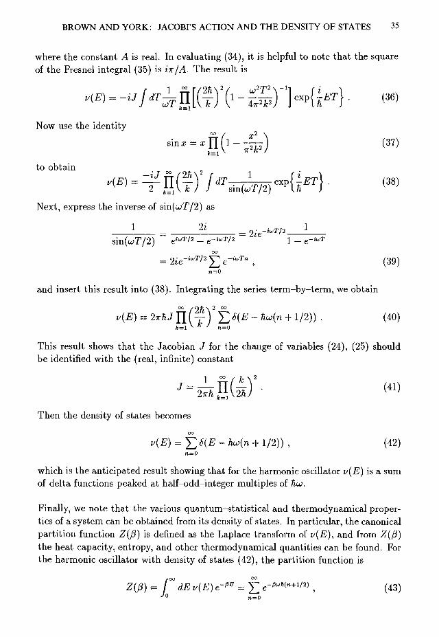
BROWN AND YORK: JACOBFS ACTION AND THE DENSITY OF STATES 35
where the constant A is real. In evaluating (34), it is helpful to note that the squareof the Fresnel integral (35) is in/A. The result is
Now use the identity
to obtain
n f ? ) f^ K k J J
fdT^ n f ? ) fdT • (2 ^K k J J sm(
Next, express the inverse of sin(u>T/2) as=»,-«/..
sm{uT/2) e -CO
= 2ie-iuT/2J2e~iuTn , (39)
and insert this result into (38). Integrating the series term-by-term, we obtain
n ( T ) ^k=1\ k J n =
This result shows that the Jacobian J for the change of variables (24), (25) shouldbe identified with the (real, infinite) constant
Then the density of states becomes
1/2)), (42)n = 0
which is the anticipated result showing that for the harmonic oscillator v(E) is a sumof delta functions peaked at half-odd-integer multiples of UL:.
Finally, we note that the various quantum-statistical and thermodynamical proper-ties of a system can be obtained from its density of states. In particular, the canonicalpartition function Z(f3) is defined as the Laplace transform of v{E), and from Z(f3)the heat capacity, entropy, and other thermodynamical quantities can be found. Forthe harmonic oscillator with density of states (42), the partition function is
fOQ OO
— / dhv[b)e = 2^,e \ (43)J 0 n
36 BROWN AND YORK: JACOBI'S ACTION AND THE DENSITY OF STATES
which is the well known result.
ACKNOWLEDGMENTSThis research was supported by National Science Foundation grant PHY-8908741.
REFERENCES
Braden, H. W., J. D. Brown, B. F. Whiting, and J. W. York (1990). Charged blackhole in a grand canonical ensemble. Physical Review, D42, 3376-3385.
Brown, J. D. and J. W. York (1989). Jacobi's action and the recovery of time ingeneral relativity. Physical Review, D40, 3312-3318.
Brown, J. D., G. L. Comer, E. A. Martinez, J. Melmed, B. F. Whiting, and J. W.York (1990). Thermodynamic ensembles and gravitation. Classical and QuantumGravity, 7, 1433-1444.
Brown, J. D., E. A. Martinez, and J. W. York (1991a). Rotating black holes, complexgeometry, and thermodynamics. In Nonlinear Problems in Relativity and Cosmol-ogy, Eds J. R. Buchler, S. L. Detweiler, and J. R. Ipser. New York Academy ofSciences, New York.
Brown, J. D., E. A. Martinez, and J. W. York (1991b). Complex Kerr-Newmangeometry and black hole thermodynamics. Physical Review Letters, 66, 2281-2284.
Brown, J. D. and J. W. York (1992). Quasi-local energy in general relativity. InMathematical Aspects of Classical Field Theory, Eds M. J. Gotay, J. E. Marsden,and V. E. Moncrief. American Mathematical Society, Providence.
Brown, J. D. and J. W. York (1993a). Quasilocal energy and conserved chargesderived from the gravitational action. To appear in Physical Review, D47.
Brown, J. D. and J. W. York (1993b). Microcanonical functional integral for thegravitational field. To appear in Physical Review, D47.
Feynman, R. P. and A. R. Hibbs (1965). Quantum Mechanics and Path Integrals.McGraw Hill, New York.
Lanczos, C. (1970). The Variational Principles of Mechanics. University of Toronto

BROWN AND YORK: JACOBFS ACTION AND THE DENSITY OF STATES 37
Press, Toronto.
Whiting, B. F. and J. W. York (1988). Action principle and partition function forthe gravitational field in black-hole topologies. Physical Review Letters, 61, 1336-1339.
York, J. W. (1986). Black-hole thermodynamics and the Euclidean Einstein action.Physical Review, D33, 2092-2099.

Decoherence of Correlation Histories
Esteban Calzetta * B. L. Hu *
Abstract
We use a A$4 scalar quantum field theory to illustrate a new approach tothe study of quantum to classical transition. In this approach, the decoherencefunctional is employed to assign probabilities to consistent histories denned interms of correlations among the fields at separate points, rather than the fielditself. We present expressions for the quantum amplitudes associated with suchhistories, as well as for the decoherence functional between two of them. Thedynamics of an individual consistent history may be described by a Langevin-type equation, which we derive.
Dedicated to Professor Brill on the occasion of his sixtieth birthday, August 1993
1. Introduction
1.1. Interpretations of Quantum Mechanics and Paradigmsof Statistical Mechanics
This paper attempts to bring together two basic concepts, one from the foundationsof statistical mechanics and the other from the foundations of quantum mechanics,for the purpose of addressing two basic issues in physics:1) the quantum to classical transition, and2) the quantum origin of stochastic dynamics.Both issues draw in the interlaced effects of dissipation, decoherence, noise, and fluc-tuation. A central concern is the role played by coarse-graining -the naturalness of itschoice, the effectiveness of its implementation and the relevance of its consequences.On the fundations of quantum mechanics, a number of alternative interpretationsexists, e.g., the Copenhagen interpretation, the many-world interpretation [1], theconsistent history interpretations [2], to name just a few (see [3] for a recent review).The one which has attracted much recent attention is the decoherent history approach
*IAFE, cc 167, sue 28, (1428) Buenos Aires, Argentina* Department of Physics, University of Maryland, College Park, MD 20742, USA
38

CALZETTA AND HU: DECOHERENCE OF CORRELATION HISTORIES 39
of Gell-Mann and Hartle [4]. In this formalism, the evolution of a physical system isdescribed in terms of 'histories': A given history may be either exhaustive (defininga complete set of observables at each instant of time) or coarse-grained. While inclassical physics each history is assigned a given probability, in quantum physics aconsistent assignment of probabilities is precluded by the overlap between differenthistories. The decoherence functional gives a quantitative measure of this overlap;thus the quantum to classical transition can be studied as a process of "diagonaliza-tion" of the decoherence functional in the space of histories.
On the foundational aspects of statistical mechanics, two major paradigms are oftenused to describe non-equilibrium processes (see, e.g., [5, 6, 7, 8]): the Boltzmanntheory of molecular kinetics, and the Langevin (Einstein-Smoluchowski) theory ofBrownian motions. The difference between the two are of both formal and conceptualcharacter.
To begin with, the setup of the problem is different: In kinetic theory one studies theoverall dynamics of a system of gas molecules, treating each molecule in the system onthe same footing, while in Brownian motion one (Brownian) particle which definesthe system is distinct from the rest, which is relegated as the environment. Theterminology of 'revelant' versus 'irrevelant' variables highlights the discrepancy.
The object of interest in kinetic theory is the (one-particle) distribution function (orthe nth-order correlation function), while in Brownian motion it is the reduced densitymatrix. The emphasis in the former is the correlation amongst the particles, while inthe latter is the effect of the environment on the system.
The nature of coarse-graining is also very different: in kinetic theory coarse-grainingresides in the adoption of the molecular chaos assumption corresponding formallyto a truncation of the BBGKY hierarchy, while in Brownian motion it is in theintegration over the environmental variables. The part that is truncated or 'ignored'is what constitutes the noise, whose effect on the 'system' is to introduce dissipationin its dynamics. Thus the fluctuation-dissipation relation and other features.
Finally the philosophy behind these two paradigms are quite different: In Brownianmotion problems, the separation of the system from the environment is prescribed:it is usually determined by some clear disparity between the two systems. Thesemodels represent "autocratic systems", where some degrees of freedom are morerelevant than others. In the lack of such clear distinctions, making a separation 'byhand' may seem rather ad hoc and unsatisfactory. By contrast, models subscribingto the kinetic theory paradigm represent "democratic systems": all particles in agas are equally relevant. Coarse-graining in Boltzmann's kinetic theory appears lesscontrived, because information about higher correlation orders usually reflects thedegree of precision in a measurement, which is objectively definable.
In the last five years we have explored these two basic paradigms of non-equilibrium

40 CALZETTA AND HU: DECOHERENCE OF CORRELATION HISTORIES
statistical mechanics in the framework of interacting quantum field theory with theaim of treating dissipative processes in the early universe [9, 10] and decoherenceprocesses in the quantum to classical transition issue [11]. Here we have begun toexplore the issues of decoherence with the kinetic model.
Because of the difference in approach and emphasis between these two paradigms andin view of their fundamental character, it is of interest to build a bridge between them.We have recently carried out such a study with quantum fields [12]. By delineatingthe conditions under which the Boltzmann theory reduces to the Langevin theory,we sought answers to the following questions:1) What are the factors condusive to the evolution of a 'democratic system' to an'autocratic system' and vise versa ? A more natural set of criteria for the separationof the system from the environment may arise from the interaction and dynamics ofthe initial closed system [13, 14].2) The construction of collective variables from the basic variables, the descriptionof the dynamics of the collective variables, and the depiction of the behavior of acoarser level of structure emergent from the microstructures. [13, 15, 16].
The paradigm of quantum open systems described by quantum Brownian models hasbeen used to analyze the decoherence and dissipation processes, for addressing basicissues like quantum to classical transitions, fluctuation and noise, particle creationand backreaction, which arise in quantum measurement theory [17, 18, 19], macro-scopic quantum systems [20], quantum cosmology [21] (for earlier work see referencesin [22]), semiclassical gravity [23, 24, 25], and inflationary cosmology [26]. The readeris referred to these references and references therein for a description of this line ofstudy.
The aim of this paper is to explore the feasibility for addressing the same set ofbasic issues using the kinetic theory paradigm. We develop a new approach basedon the application of the decoherence functional [2, 4] formalism to histories definedin terms of correlations between the fundamental field variables. We shall analysethe decoherence between different histories of an interacting quantum field, a A$4
theory here taken as example, corresponding to different particle spectra and studyissues on the physics of quantum to classical transition, the relation of decoherenceto dissipation, noise and fluctuation, and the quantum origin of classical stochasticdynamics.
1.2. Quantum to Classical Transition and Coarse-Graining
One basic constraint in the building of quantum theory is that it should reproduceclassical mechanics in some limit. (For a schematic discussion of the different criteriaof classicality and their relations, see [27]). Classical behavior can be characterizedby the existence of strong correlations between position and momentum variables

CALZETTA AND HU: DECOHERENCE OF CORRELATION HISTORIES 41
described by the classical equations of motion [28] and by the absense of interferencephenomena (decoherence).
Recent research in quantum gravity and cosmology have focussed on the issue of quan-tum to classical transition. This was highlighted by quantum measurement theory forclosed systems (for a general discussion, see, e.g., [29]), the intrinsic incompatibilityof quantum physics with general relativity [30], and the quantum origin of classicalfluctuations in explaining the large scale structure of the Universe. Indeed, in theinflationary models of the Universe [31], one hopes to trace all cosmic structures tothe evolution from quantum perturbations in the inflaton field. More dramatically,in quantum cosmology [32] the whole (classical) Universe where we now live in isregarded as the outcome of a quantum to classical transition on a cosmic scale. Inthese models, one hopes not only to explain the 'beginning' of the universe as aquantum phenomenon, but also to account for the classical features of the presentuniverse as a consequence of quantum fluctuations. This requires not only a theoreti-cal understanding of the quantum to classical transition issue in quantum mechanics,but also a theoretical derivation of the laws of classical stochastic mechanics fromquantum mechanics, the determination of the statistical properties of classical noise(e.g., whether it is white or coloured, local or nonlocal) being an essential step in theformulation of a microscopic theory of the structure of the Universe [26].
Our understanding of the issue of quantum to classical transition has been greatlyadvanced by the recent development of the decoherent histories approach to quantummechanics [4]. An essential element of the decoherent histories approach is that theoverlap between two exhaustive histories can never vanish. Therefore, the discussionof a quantum to classical transition can only take place in the framework of a coarsegrained description of the system, that is, giving up a complete specification of thestate of the system at any instant of time.
As a matter of fact, some form of coarse graining underlies most, if not all, successfulmacroscopic physical theories. This fact has been clearly recognized and exploited atleast since the work of Nakajima and Zwanzig [33, 6] on the foundations of nonequi-librium statistical mechanics. Like statistical mechanics, the decoherent historiesapproach allows a variety of coarse-graining procedures; not all of these, however, areexpected to be equally successful in leading to interesting theories. Since the pre-scription of the coarse graining procedure is an integral part of the implementation ofthe decoherent histories approach, the development and evaluation of different coarsegraining strategies is fundamental to this research program.
When we survey the range of meaningful macroscopic (effective) theories in physicsarising from successfully coarse-graining a microscopic (fundamental) theory, one par-ticular class of examples is outstanding; namely, the derivation of the hydrodynamicaldescription of dilute gases from classical mechanics. The crucial step in deriving theNavier-Stokes equation for a dilute gas consists in rewriting the Liouville equation

42 CALZETTA AND HU: DECOHERENCE OF CORRELATION HISTORIES
for the classical distribution function as a BBGKY hierarchy, which is then truncatedby invoking a 'molecular chaos' assumption. If the truncation is made at the levelof the two-particle reduced distribution function, the Boltzmann equation results. Inthe near-equilibrium limit, this equation leads to the familiar Navier-Stokes theory.
We must stress that in this general class of theories exemplified by Boltzmann's work,coarse-graining is introduced through the truncation of the hierarchy of distributionfunctions; i.e., by neglecting correlations of some order and above at some singled-outtime [5, 6]. This type of coarse graining strategy is qualitatively different from thoseused in most of the recent work in quantum measurement theory and cosmology,which invoke a system-bath, space-time, or momentum-space separation. In most ofthese cases, an intrinsically justifiable division of the system from the environment islacking and one has to rely on case-by-case physical rationales for making such splits.(An example of system-bath split is Zurek's description of the measurement processin quantum mechanics, where a bath is explicitly included to cause decoherence inthe system-apparatus complex [17]. Space-time coarse graining has been discussedby Hartle [34] and Halliwell et al [35]. An example of coarse-graining in momentumspace is stochastic inflation [36], where inflaton modes with wavelenghts shorter thanthe horizon are treated as an environment for the longer wavelenght modes [37]).
1.3. Coarse-Graining in the Hierarchy of Correlations
In this paper we shall develop a version of the decoherent histories approach where thecoarse-graining procedure is patterned after the truncation of the BBGKY hierarchyof distribution functions. For simplicity, we shall refer below to the theory of a singlescalar quantum field, with a A$4- type nonlinearity.
The simplest quantum field theoretical analog to the hierarchy of distribution func-tions in statistical mechanics is the sequence of Green functions (that is, the expec-tation values of products of n fields) [9]. In this approach, the BBGKY hierarchyof kinetic equations is replaced by the chain of Dyson equations, linking each Greenfunction to other functions of higher order.The analogy between these two hierarchies is rendered most evident if we introduce"distribution functions" in field theory through suitable partial Fourier transforma-tion of the Green functions. Thus, a "Wigner function" [38] may be introduced asthe Fourier transform of the Hadamard function (the symmetric expectation valueof the product of two fields) with respect to the difference between its arguments. Itobeys both a mass shell constraint and a kinetic equation, and may be regarded asthe physical distribution function for a gas of quasi particles, each built out of a cloudof virtual quanta. Similar constructs may be used to introduce higher "distributionfunctions" [9, 7].
As in statistical mechanics, the part of a given Green function which cannot be re-

CALZETTA AND HU: DECOHERENCE OF CORRELATION HISTORIES 43
duced to products of lower functions defines the corresponding "correlation function".Thus the chain of Green functions is also a hierarchy of correlations.
To establish contact between the hierarchy of Green functions and the decoherenthistories approach, let us recall the well-known fact that the set of expectation valuesof all field products contains in itself all the information about the statistical stateof the field [9]. For a scalar field theory with no symmetry breaking, we can evennarrow this set to products of even numbers of fields. This result suggests thata history can be described in terms of the values of suitable composite operators,rather than those of the fundamental field. If products to all orders are specified(binary, quartet, sextet, etc), then the description of the history is exhaustive, anddifferent histories do not decohere. On the other hand, when some products are notspecified, or when the information of higher correlations are missing, which is oftenthe case in realistic measurement settings, the description is coarse-grained, whichcan lead to decoherence.
In this work we shall consider coarse-grained histories where the lower field prod-ucts (binary, quartic) are specified, and higher products are not. Decoherence willmean that the specified composite operators can be assigned definite values with con-sistent probabilities. Higher composite operators retain their quantum nature, andtherefore cannot be assigned definite values. However, their expectation values canbe expressed as functionals of the specified correlations by solving the correspond-ing Dyson equations with suitable boundary conditions. This situation is exactlyanalogous to that arising from the truncated BBGKY hierarchy, where the molecularchaos assumption allows the expression of higher distribution functions as functionalsof lower ones ( e.g., [5, 6]).
For those products of fields which assume definite values with consistent probabili-ties, these values can be introduced as stochastic variables in the dynamical equa-tions for the other quantities of interest (usually of lower correlation order). Thisapproach would provide a theoretical basis for the derivation of the equations ofclassical stochastic dynamics from quantum fields. It can offer a justification (orrefutation) for a procedure commonly assumed but never proven in some populartheories like stochastic inflation [36, 37]. Moreover, since in general we shall obtainnontrivial ranges of values for the specified products with nonvanishing probabili-ties, it can be said that our procedure captures both the average values of the fieldproducts and the fluctuations around this average. The statistical nature of thesefluctuations is a subject of great interest in itself [26].
There is another conceptual issue that our approach may help to clarify. As we havealready noted, in the system-bath split approach to coarse-graining, as well as in re-lated procedures, it is crucial to introduce a hierarchical order among the degrees offreedom of the system, in such a way that some of them may be considered relevant,and others irrelevant. While it is often the case that the application itself suggests

44 CALZETTA AND HU: DECOHERENCE OF CORRELATION HISTORIES
which notions of relevance may lead to an interesting theory, in a quantum cosmo-logical model, which purports to be a "first principles" description of our Universe,all these choices are, in greater or lesser degree, arbitrary. Since correlation functionsalready have a "natural" built-in hierarchical ordering, in this approach the 'arbi-trariness' is reduced to deciding on which level this hierarchy is truncated, and thatin turn is determined by the degree of precision one carries out the measurement. Inmost case one still needs to show the robustness of the macroscopic result against thevariance of the extent of coarse-graining, and exceptional situations do exists (an ex-ample is the long time-tail relaxation behavior in multiple particle scattering of densegas, arising from a failure of the simple molecular chaos assumption). But in generalterms correlational coarse-graining seems to us a less ad hoc procedure compared tothe commonly used system-bath splitting and coarse-graining.
This paper is organized as follows: In Sec. 2 we discuss the implementation of ourprocedure for the simple case of a A3>4 theory in flat space time. We then derivethe formulae for the quantum amplitude associated with a set of correlation historiesand the decoherence functional between two such histories. In Sec. 3 we discuss thedecoherence of correlation histories between binary histories and derive the classicalstochastic source describing the effect of higher-order correlations on the lower-orderones, arriving at a Langevin equation for classical stochastic dynamics. In Sec. 4 wesummarize our findings.
2. Quantum Amplitudes for Correlation Histories and Ef-fective Action
2.1. Quantum Mechanical Amplitudes for Correlation His-tories
In this section, we shall consider the quantum mechanical amplitudes associated withdifferent histories for a A$4 quantum field theory, defined in terms of the values oftime-ordered products of even numbers of fields at various space time points. Let usbegin by motivating our ansatz for the amplitudes of these correlation histories.
In the conceptual framework of decoherent histories [4], the "natural" exhaustivespecification of a history would be to define the value of the field $(x) at every spacetime point. These field values are c numbers. The quantum mechanical amplitudefor a given history is \I>[$] ~ elS^\ where S is the classical action. The decoherencefunctional between two different specifications is given by D[$,$f] ~Since |Z)[$,$']| = 1, there is never decoherence between these histories.
A coarse-grained history would be defined in general through a "filter function" a,which is basically a Dirac 6 function concentrated on the set of exhaustive histo-ries matching the specifications of the coarse-grained history. For example, we may

CALZETTA AND HU: DECOHERENCE OF CORRELATION HISTORIES 45
have a system with two degrees of freedom x and t/, and define a coarse-grainedhistory by specifying the values xo(t) of x at all times. Then the filter function isa[x,t/] = Ilt€R&{%{t) — %o{t))' The quantum mechanical amplitude for the coarse-grained history is defined as
9[a] = f (1)
where the information on the quantum state of the field is assumed to have beenincluded in the measure and/or the boundary conditions for the functional integral.The decoherence functional for two coarse-grained histories is [4]
D[a,a'} = I Z>*J9*V<5<*>-5<*'»a[*]a'[*'] (2)
In this path integral expression, the two histories $ and $' are not independent; theyassume identical values on a t = T = constant surface in the far future. Thus, theymay be thought of as a single, continuous history defined on a two-branched "closedtime-path" [39, 40, 41, 42], the first branch going from t = —oo to T, the secondfrom T back to — oo. Alternatively, we can think of $ = 4>x and $' = $2 as thetwo components of a field doublet defined on ordinary space time [9], whose classicalaction is 5[$a] = S[$x] — 5[$2]. This notation shall be useful later on.
Let us try to generalize this formalism to correlation histories. We begin with thesimplest case, where only binary products are specified. In this case a history isdefined by identifying a symmetric kernel G(x,x'), which purports to be the valueof the product $(#)$(#') in the given history, both x and x1 defined in Minkowskyspace - time. By analogy with the formulation above, one would write the quantummechanical amplitude for this correlation history as
eiS I ] 6($(x)${xf)-G(x,x')) (3)
(In this equation, we have introduced a formal ordering of points in Minkowsky space- time, simply to avoid counting the same pair twice.)
But this straightforward generalization for the correlation history amplitude is un-satisfactory on at least two counts. First, it assumes that the given kernel G canactually be decomposed (maybe not uniquely) as a product of c number real fieldsat different locations; however, we wish to define amplitudes for kernels (such as theFeynman propagator) which do not have this property. Second, (which is relatedto the first point,) it is ambiguous, since we do not have a unique way to expresshigher even products of fields in terms of binary products, and thus of applying the6 function constraint.

46 CALZETTA AND HU: DECOHERENCE OF CORRELATION HISTORIES
To give an example of this, observe that, should we expand the exponential of the ac-tion in powers of the coupling constant A, the second order term / dx dx1 $(x)4$(x')4
could become, after integration over the delta function, either
dxdx' G{x,x)2G(x',x')\
dxdx' G{x,x')\
(4)
or any other combination; of course, if G could be decomposed as a product of fields,this would be unimportant.
Let us improve on these shortcomings. The general idea is to accept Eq. (3) as thedefinition of the amplitude in the restricted set of kernels where it can be applied, andto define the amplitude for more general kernels through some process of analyticalcontinuation. To this end, we must rewrite the quantum mechanical amplitude in amore transparent form, which we achieve by using an integral representation of the8 function. Concretely, we redefine
DK eWr[K]-{i/*)Ka) (6)
9[G\ = f DK f D$ jS+ijdxdx' K{x,x')(*(x)*{x')-G{x,x')) ^
where the filter function in the Gell-Mann Hartle scheme is replaced by an integrationover "all" symmetric non-local sources K. Eq. (5) is not yet a complete definition,since one must still specify both the path and the measure to be used in the Kintegration. Performing the integration over fields, we obtain
*[(?] = Jwhere W[2f] is the generating functional for connected vacuum graphs withinteraction, and (A""1 — K)~x for propagator (see below). Here A"1 = —V 2 + m2 isthe free propagator for our scalar field theory (our sign convention for the flat space- time metric is —h ++).
The path integral over kernels can be computed through functional techniques. Forexample, for a free field, A = 0,
W[K] = - i lnDet^A"1 - K)~1/2] + constant (7)
Through the change of variables
(A"1 - K) = KG-1 (8)we obtain

CALZETTA AND HU: DECOHERENCE OF CORRELATION HISTORIES 47
= constant [Det G]"1/2 e^i/2^A'lG (9)
When the self coupling A is not zero, the evaluation of 9[G] is more involved; however,if we are interested in the leading behavior of the amplitude only, we can simplyevaluate the functional integral over K by saddle point methods. The saddle lies atthe solution to
1= 2°
We recognize immediately that the exponent, evaluated at the saddle point, is simplythe 2 Particle Irreducible (2PI) effective action F, with G as propagator (see below).Including also the integration on gaussian fluctuations around the saddle, we find
(11)
This is our main result.As a check, it is interesting to compare the saddle method expression with our exactresult for free fields. For a free field T[G] = (-i'/2)lnDet(G) - (1/2)A-1G, andtherefore T,G = {-il2){G~l - iA"1), T,GiG = (i/2)G~2, so
(12)
which is exactly the earlier result, Eq. (9).
2.2. Quantum Amplitudes and Effective Actions
Eq. (11) is the natural generalization to correlation histories of the quantum me-chanical amplitude elS associated to a field configuration. Let us consider its physicalmeaning.
The effective action is usually introduced in Field Theory books [43] as a compactdevice to generate the Feynman graphs of a given theory. Indeed, all Feynman graphsappear in the expansion of the generating functional
Z[J] = I D$e^5+J*) (13)in powers of the external source J [here, «/$ = / d Ax J(x)$(x)]. Z has the physicalmeaning of a vacuum persistance amplitude: it is the amplitude for the in vacuum(that is, the vacuum in the distant past) to evolve into the out vacuum (the vacuum

48 CALZETTA AND HU: DECOHERENCB OF CORRELATION HISTORIES
in the far future) under the effect of the source J. Thus, after proper normalization,\Z\ will be unity when the source is unable to create pairs out of the vacuum, andless than unity otherwise.
A more compact representation of the Feynman graphs is provided by the functionalW[J] = — i lnZ[J ] ; the Taylor expansion of W contains only connected Feynmangraphs. Thus W developing a (positive) imaginary part signals the instability of thevacuum under the external source J .
The external source will generally drive the quantum field $ so that its matrix element
(Oout|*(»)|0tn)* x ) = (Oout\0in)
between the in and out vacuum states will not be zero. Indeed, it is easy to see that
The transformation from J to <f> is generally one to one, and thus it is possible toconsider the matrix element, and not the source, as the independent variable. This isachieved by submitting W to a Legendre transformation, yielding the effective actionT[<j>] = W[J] — J<f> [J and <j> being related through Eq. (15)]. This equation can beinverted to yield the dynamic law for </>
Eq. (16) shows that F may be thought of as a generalization of the classical action,now including quantum effects. In the absence of external sources, the in and outvacua agree, so <f> becomes a true expectation value; its particular value is found byextremizing the effective action. Indeed, in this case it can be shown that F is theenergy of the vacuum.
can be defined independently of the external source through the formula [44]
T[<f>] = S[<f>) + (i/2)lnDet ( 0 ) + 1 ^ ] (17)
where Fi represents the sum of all one particle irreducible (1PI) vacuum graphs ofan auxiliary theory whose classical action is obtained from expanding the classicalaction S[</> + (p] in powers of <p, and deleting the constant and linear terms. Eq. (17)shows that F is related to the vacuum persistance amplitude of quantum fluctuationsaround the matrix element <j>. Therefore, an imaginary part in F also signals avacuum instability. This situation closely resembles the usual approach to tunneling

CALZETTA AND HU: DECOHERENCE OF CORRELATION HISTORIES 49
and phase transitions, where an imaginary part in the free energy signals the onsetof instability [45].
Observe that each of the transformations from Z to W to F entails a drastic sim-plification of the corresponding Feynman graphs expansions, from all graphs in Z toconnected ones in W and to 1PI ones in F. Roughly speaking, it is unneccessary toinclude non 1PI graphs in the effective action, because the sum of all one-particleinsertions is already prescribed to add up to <f>. Now the process can be continued:if we could fix in advance the sum of all self energy parts, then we could write downa perturbative expansion where only 2PI Feynman graphs need be considered. Thisis achieved by the 2PI effective action [46].
Let us return to Eq. (13), and add to the external source a space-time dependentmass term
Z[J,K] =
where $K$ = / dx dx' ${x)K{x,x')$(x'). Also define W[J,K] = -ilnZ[J,K}.Then the variation of W with respect to J defines the in-out matrix element of thefield, as before, but now we also have
(19)dK(x,x>) 2^"'^"'
where GF represents the Feynman propagator of the quantum fluctuations <p aroundthe matrix element <f>. As before, it is possible to adopt G as the independent variable,instead of K. To do this, we define the 2PI effective action (in schematic notation)T[<f>,GF] = W[J,K] - J<j>- {l/2)K[<f>2 + GF]. Variation of this new F yields theequations of motion F ^ = — J — K<f>, TtaP — ( — 1/2)K.
We can see that the 2PI effective action generates the dynamics of the Feynmanpropagator, and in this sense it plays for it the role that the classical action plays forthe field. In this sense we can say that Eq. (11) generalizes the usual definition ofquantum mechanical amplitudes.
The perturbative expansion of the 2PI effective action reads [46]
T[+,GF] - S[4>] + (;/2)lnDetG^ + (\) T r ( 0 G F ) + T2[<t>yGF) + constant (20)
where F2 is the sum of all 2PI vacuum graphs of the auxiliary theory already consid-ered, but with GF as propagator in the internal lines. As we anticipated, to replaceGF for the perturbative propagator amounts to adding all self energy insertions, andtherefore no 2PI graph needs be explicitly included.

50 CALZETTA AND HU: DECOHERENCE OF CORRELATION HISTORIES
Like its 1PI predecessor, the 2PI effective action has the physical meaning of a vac-uum persistence amplitude for quantum fluctuations y?, constrained to have vanishingexpectation value and a given Feynman propagator. Therefore, an imaginary part inthe 2PI effective action also signals vacuum instability.
The description of the dynamics of a quantum field through both <j) and Gp simulta-neously, rather than <f> alone, is appealing not only because it allows one to performwith little effort the resummation of an infinite set of Feynman graphs, but also be-cause for certain quantum states, it is possible to convey statistical information aboutthe field through the nonlocal source K. This information is subsequently transferredto the propagator. For this reason, the 2PI effective action formalism is, in our opin-ion, a most suitable tool to study statistical effects in field theory, particularly forout-of-equilibrium fields [9, 47]. In our earlier studies the object of interest is theon-shell effective action, that is, the effective action for propagators satisfying theequations of motion. Here, in Eq. (11), we find a relationship between the quantummechanical amplitude for a correlation history and the 2PI effective action whichdoes not assume any restriction on the propagator concerned.
2.3. Quantum Amplitudes for More General CorrelationHistories: 2PI CTP Effective Action
One of the peculiarities of the ansatz Eq.(3) for the amplitude of a correlation his-tory is that the kernel G must be interpreted as a time - ordered binary product offields. This results from the known feature of the path integral, which automaticallytime orders any monomials occurring within it. Before we proceed to introduce thedecoherence functional for correlation histories, it is convenient to discuss how thisrestriction could be lifted, as well as the restriction to binary products.
The time ordering feature of the path integral is also responsible for the fact thatthe c-number field <j> in Sec. 2.2 is a matrix element, rather than a true expectationvalue. As a matter of fact, the Feynman propagator GF discussed in the previoussection is also a matrix element
(O0ut\T[<p(x)<p(x')}\Oin)GF{X> X } =
Because <j> and Gp satisfy mixed boundary conditions, the dynamic equations result-ing from the 2PI effective action are generally not causal. This drawback has placedlimitations in their physical applications.
Schwinger [39] has introduced an extended effective action, whose arguments aretrue expectation values with respect to some in quantum state. Because the dynam-ics of these expectation values may be formulated as an initial value problem, the

CALZETTA AND HU: DECOHERENCE OF CORRELATION HISTORIES 51
equations of motion resulting from the Schwinger-Keldysh effective action are causal.Schwinger's idea is also the key to solving the restrictions in our definition of quantumamplitudes for correlation histories.Schwinger's insight was to apply the functional formalism we reviewed in Sec. 2.2 tofields defined on a "closed time-path", composed of a "direct" branch — T < t < T,and a "return" branch T > t > -T (with T -> oo) [39, 40]. Actually, we havealready encountered this kind of path in the discussion of the decoherence functionalfor coarse - grained histories. Since the path doubles back on itself, the in vacuum isthe physical vacuum at both ends; the formalism may be generalized to include moregeneral initial states, but we shall not discuss this possibility[9].
The closed time-path integral time-orders products of fields on the direct branch, anti-time-orders fields on the return branch, and places fields on the return branch alwaysto the left of fields in the direct branch. To define the closed time-path generatingfunctional, we must introduce two local sources Ja, and four nonlocal ones Kab (asin Sec. 2.1 an index a, 6 = 1 denotes a point on the first branch, while an index2 denotes a point on the return part of the path). These sources are conjugatedto c number fields <fia and propagators Gab, which stand for (0in\$a(x)\Qin) and(0in\<pa(x)(pb(xf)]\0in). Explicitly, decoding the indices, the propagators are definedas (here and from now on, we assume that the background fields (f>a vanish):
) (22)
, x') = (0m|*(^)*(aj)|0m) (23)
, x') = (0in|$(^)$(^)|0m) (24)
G22{x,x') = (0in\(T[Q{x)*(x')]y\0in) (25)
They are, respectively, the Feynman, negative- and positive- frequency Wightman,and Dyson propagators. The definition of the closed time-path (CTP) or in-in 2PIeffective action follows the same steps as the ordinary effective action discussed inthe previous section, except that now, besides space-time integrations, one must sumover the discrete indexes a, 6. These indexes can be raised and lowered with the"metric" h^ = diag(l,—1). Similarly, the "propagator" to be used in Feynmangraph expansions is the full matrix Gah, and the interaction terms should be read outof the CTP classical action 5[$1] - S[$2], discussed in Sec. 2.1.In the case of vacuum initial conditions, these can be included into the path integralby tilting the branches of the CTP in the complex t plane (the direct branch should

52 CALZETTA AND HU: DECOHERENCE OF CORRELATION HISTORIES
acquire an infinitesimal positive slope, and the return branch, a negative one [48]).The CTP boundary condition, that the histories at either branch should fit continu-ously at the surface t = T, may also be explicitly incorporated into the path integralas follows. We first include under the integration sign a term
II 8($\x,T)-$\x,T)) (26)xeR>
which enforces this boundary condition; then we rewrite Eq.(26) as
exp{(-l/a')J d*x (^(x,T)-^(x,T))2} (27)
where a —» 0. This term has the form
exp{i f d4x d4x'Kab(x,x')$a{x)$b(x')}, (28)
where
Kab{x, x') = {i/a2)S(x - x')6(t - T)[2Sab - 1]. (29)
In this way, we have traded the boundary condition by an explicit coupling to a nonlocal external source.
As before, variation of the CTP 2PI effective action yields the equations of motionfor background fields and propagators. The big difference is that now these equationsare real and causal [42, 9].
We can now see how the CTP technique solves the ordering problem in the definitionof quantum amplitudes for correlation histories. One simply considers the specifiedkernels as products of fields defined on a closed time - path. In this way, we may defineup to four different kernels Gab independently, to be identified with the four differentpossible orderings of the fields (for simplicity, we assume the background fields arekept equal to zero). If the kernels Gab can actually be decomposed as products ofc-number fields on the CTP, then we associate to them the quantum amplitude
ab] = f D$a eiS H 6($a(x)$b{x')-Gab(x7x')) (30)x>x',ab
(where S stands for the CTP classical action) The path integral can be manipulatedas in Sec. 2.1 to yield

CALZETTA AND HU: DECOHERENCE OF CORRELATION HISTORIES 53
where F stands now for the CTP 2PI effective action. This last expression canbe analytically extended to more general propagator quartets, and, indeed, even tokernels which do not satisfy the relationships Gu(xyxf) = G21(x,x') = G12*(x,x') =G22*(«r, x 1) for t > t'y which follow from their interpretation as field products.
Quantum amplitudes for correlation histories including higher order products aredefined following a similar procedure. For example, four particle correlations arespecified by introducing 16 kernels [9]
gabcd $a$b$c^d _ gabgcd _ gacgbd _ gadgbc /g2)
If the new kernels are simply products of the binary ones, then the amplitude is givenby
b fiabcdl _ I n&a AS TT ^ * a A & r*aby[Gab,Gabcd] = D$ a elS J j£ ($ a $ 6 - Gab)J ab
TT ^($a$f e$c$r f _ GabGcd — GacGbd — GadGbc — Gabcd)abed
(33)
(In the last two equations, we have included the space - time index x and the branchindex a into a single multi index). Here, each pair appears only once in the product,as well as each quartet abed. Exponentiating the 8 functions we obtain
Gahcd) = J DKabcd J DKah J D$ exp{i[S + ^
K($a$b$c$d - GabGcd - GacGw - GadGhc - Gabcd)]}
(34)
Now the integral over fields yields the CTP generating functional for connectedgraphs, for a theory with a non local interaction term. Thus
= j DKahcd j DKab exp{i[W[Kab, Kabcd] - l-KabGab
-^Kabcd{GabGcd + GacGM + G^G* + Gabcd)}}Z4
(35)
The integral may be evaluated by saddle point methods, the saddle being the solutionto W}Kab = (l/2)Gab, W)Kabcd = ±(GabGcd + GacGbd + GadGbc + Gabcd). To evaluatethe exponential at the saddle is the same as to perform a Legendre transform onW -it yields the higher order CTP effective action T[Gab, Gabcd). Variation of F yieldsthe equation of motion for its arguments, which are also the inversion of the saddle

54 CALZETTA AND HU: DECOHERENCE OF CORRELATION HISTORIES
point conditions
r c - = (-l/2)Kab - (l/4)KabcdGcd
(36)
Thus up to quartic correlations, the quantum mechanical amplitude is given by
This expression can likewise be extended to more general kernels.
As a check on the plausibility of this result, let us note the following point. Sincequantum mechanical amplitudes are additive, it should be possible to recover ourearlier ansatz Eq. (11) for binary correlation histories from the more general resultEq. (37), by integration over the fourth order kernels. Within the saddle pointapproximation, integration amounts to substituting these kernels by the solutionto the second Eq. (36) for the given (?ob, with K^^ = 0, and with null initialconditions. (Indeed, since initial conditions can always be included as delta function- like singularities in the external sources, the third condition is already included inthe second.) This procedure effectively reduces the fourth order effective action tothe 2PI CTP one [9], as we expected.
A basic point which emerges here relevant to our study of decoherence is that , whilequantum field theory is unitary and thus time reversal invariant, the evolution ofthe propagators derived from the 2PI CTP effective action is manifestly irreversible[9, 49]. The key to this apparent paradox is that , while the evolution equations areindeed time reversal invariant, when higher order kernels are retained as indepen-dent variables, their reduction to those generated by the 2PI effective action involvesthe imposition of trivial boundary conditions in the past. Thus the origin of irre-versibility in the two point functions is the same as in the BBGKY formulation instatistical mechanics [5]. The lesson for us in the present context is that there is anintrinsic connection between dissipation and decoherence [26, 23]. Knowledge thatthe evolution of the propagators generated by the 2PI effective action is generallydissipative leads us to expect that histories defined through binary correlations willusually decohere. We proceed now to a detailed study of this point.

CALZETTA AND HU: DECOHERENCE OF CORRELATION HISTORIES 55
3. Decoherence of Correlation Histories
3.1, Decoherence Functional for Correlation Histories
Having found an acceptable ansatz for the quantum mechanical amplitude associatedwith a correlation history, we are in a position to study the decoherence functionalbetween two such histories. As was discussed in the Introduction, if the decoherencefunctional is diagonal, then correlation histories support a consistent probability as-signment, and may thus be viewed as classical (stochastic) histories.
For concreteness, we shall consider the simplest case of decoherence among historiesdefined through (time-ordered) binary products. Let us start by considering twohistories, associated with kernels G(xyx') and (?'(#, #'), which can in turn be writtenas products of fields. Taking notice of the similarity between the quantum amplitudesEqs. (1) and (3), we can by analogy to Eq. (2) define the decoherence functional forsecond correlation order as
D[G,G'} =JII *((#(*)*(*') - G(x,x'))8((nx)*V) ~ G'*(x,x'))
(38)
Recalling the expression Eq. (30) for the quantum amplitude associated with themost general binary correlation history, we can rewrite Eq. (38) as
D[G, G'] = / DG12 DG21 tf [G11 = G, G22 = G'\ G12, G21} (39)
This expression for the decoherence functional can be extended to arbitrary kernels.
In the spirit of our earlier remarks, we use the ansatz Eq. (31) for the CTP quantumamplitude and perform the integration by saddle point methods to obtain
D[G, G'} ~ e'r[G"=G,G"=G",Gj>,G2M ( 4 0 )
where the Wightman functions are chosen such that
91 9T = 0 (41)
for the given values of the Feynman and Dyson functions. These last two equationsare the sought-for expression for the decoherence functional.As an application, let us study the decoherence functional for Gaussian fluctuationsaround the vacuum expectation value (VEV) of the propagators for a A$4 theory,

56 CALZETTA AND HU: DECOHERENCE OF CORRELATION HISTORIES
carrying the calculations to two-loop accuracy. Gaussian fluctuations means that weonly need the closed time-path 2PI effective action to second order in the fluctuations8Gah = Gab - Ag6, where Af stands for the VEVs. Since the effective action isstationary at the VEV, there is no linear term. Formally
T[8Gab] = (l/2){T,{aaUbb)SGaaSGbb + 2T<{ai:hUcc)8Ga*h8Gcc + T^bU^d)8G^b8G^d}(42)
so the saddle point equations (41) become
{r,(a^),(c^)}^Go^ = -r,(a^),(ee)£GCe (43)
The formal Feynman graph expansion of the 2PI effective action is given in Eq. (20).To two-loop accuracy, we find [9]
T2{Gab) = -\habcdf d4x Gab(x,x)Gcd(x,x)
d*x d4x'Gae(x,x')Gb'(x,x')Gc°(x,x')Gdh(x,x')
(44)
where ha(,, /labcd = 1 ii a = b = c = d = 1, —1 it a = b = c = d = 2, and vanishotherwise.
Computing the necessary derivatives, we find
d2TdGab(x,x')dGcd(x",x'") ~
+(l/2)XhabedS(x' - x)S{x" - x)8{x'" - x)-(il2)X2haceghbdfj8(x" - x)8(x'" - x')Gtf(xtx')G'i(x1x')]
(45)
These derivatives are evaluated at Gab = Ajf, where
(AjJ" )ab{xj x ) = i[hab{~~V + TTl — ih ab€)S(x' — x)
+(X/2)habcd8(x'-x)Aco
d(x,x)-{i/6)X2haecdhbfghAe
of(x, x')Ac
09{x, x')Adh{x, x')}
l;8(x'-x)8(t-T)[28ab-l]2a2
(46)
where it is understood that the limits e,a —» 0, T —» oo are taken. The first in-finitesimal is included to enforce appropiate Feynman/Dyson orderings, the secondto carry the CTP boundary conditions in the far future.

CALZETTA AND HU: DECOHERENCE OF CORRELATION HISTORIES 57
In computing the Feynman graphs in these expressions, the usual divergences cropup. They may be regularized and renormalized by standard methods, which we willnot discuss here. The "tadpole" graph A%*(x,x) can be made to vanish by a suitablechoice of the renormalization point, which we shall assume.
Let us narrow our scope to a physically meaningful set of histories, namely, thosedescribing ensembles of real particles distributed with a position-independent spec-trum /(fe), k being the four momentum vector. Such ensembles are described bypropagators [9]
5G(x,x') = 2*J ( ^ j ) eife<*-*')*(fc2 + m2)/(fc) (47)
The distribution functions / are real, positive, and even in k. We wish to analyzeunder what conditions it is possible to assign consistent probabilities to differentspectra / . To this end we must compute the decoherence functional between thepropagator in Eq. (47) and another, say, associated with a function / ' .
Let us begin by investigating Eqs (43) for the missing propagators G12 and C?21.We shall first disregard the boundary condition enforcing terms in these equations,introducing them at a later stage. When this is done, the right hand side of Eqs.(43) vanishes, since (—V 2 + m2)Gaa(x,xf) = 0 in the present case.
On the other hand, we only need the left hand side to zeroth order in A, since any otherterm would be of too high an order to contribute to the decoherence functional at thedesired accuracy. With this in mind, Eq. (43) reduces to the requirement that theunknown propagators should be homogeneous solutions to the Klein-Gordon equationon both of their arguments.
To determine the proper boundary conditions for these propagators, we may considerthe boundary terms in Eq. (46), or else appeal to their physical interpretation. Weshall choose the second approach.
To this end, we observe that the physical meaning of the propagators as (non stan-dard) products of fields, Eqs. (22) to (25), entails the identity G12 + G21 = Gu + G22,which is consistent in this case, since both sides solve the Klein - Gordon equation.Actually, this identity is satisfied by the VEV propagators, so it can be imposeddirectly on their variations.
Physically, a change in the propagators reflects a corresponding change in the sta-tistical state of the field. To zeroth order in the coupling constant, however, thecommutator of two fields is a c-number , and does not depend on the state. There-fore, to this accuracy, G12 — G21 should not change; that is, 8G12 should be equal toSG21. We thus conclude that the correct solution to Eq. (43) is

58 CALZBTTA AND HU: DECOHERENCE OF CORRELATION HISTORIES
8G12 = 8G21 = (h{SGu + SG22} (48)
Consideration of the CTP boundary conditions would have led to the same result.
We may now evaluate the second variation of the 2PI CTP effective action, Eq.(42). We should stress that the Klein-Gordon operator annihilates all propaga-tors involved, and that the O(X) term in A Q 1 vanishes because of our choice ofrenormalization point. Therefore the second (mixed) term in Eq. (42) is of higherthan second order and may be disregarded. The same holds for terms of the form(A0)-*8Gcd(A0)dbSGabi disregarding boundary terms.
The remaining terms can be read out of Eq. (45), with the input of the "fish" graph[43, 9]
(49)
where e = d — 4 and fi is the renormalization scale. Clearly, the local terms in £ canbe absorbed into a coupling- constant renormalization.
The important thing for us to realize is that the O(X) terms in Eq. (45), as well as theimaginary part of S, contribute only to the phase of the decoherence functional, andthus are totally unrelated to decoherence. The only contribution to a decoherenceeffect comes from the real part of S. Reading it out of Eq. (49), we obtain the soughtfor result
\D[fJ'}\
(f(p) - f'(p))(f(q) ~ f'(q)W-((P + if + 4m2)]2 V - 4 m 2
(50)
where 0 is the usual step function. As expected, we do find decoherence betweendifferent correlation histories. Moreover, decoherence is related to dissipative pro-cesses, which in this case arise from pair production [49]. Indeed, the real part ofthe kernel S is essentially the probability of a real pair being produced out of quantawith momenta p and <?, with p + q = k [43].

CALZETTA AND HU: DECOHERENCE OF CORRELATION HISTORIES 59
Let us mention two obvious consequences of our result for the decoherence functional.The first point is that decoherence is associated with instability of the vacuum: thedistribution functions whose overlap is suppressed represent ensembles which areunstable against non trivial scattering of the constituent particles. This scatteringproduces correlations between particles. Therefore, truncation of the correlation hi-erarchy leads to an explicitly dissipative evolution. This would not be the case ifthere were no scattering.
The second point is that \D\ remains unity on the diagonal. Thus, at least forGaussian fluctuations, and to two-loop accuracy, all histories are equally likely. Whatthis means physically is that the two-point functions to be perceived by an observerafter the quantum to classical transition need not be close to their VEV in anystringent sense. Indeed, what is observed will not even be "vacuum fluctuations" inthe proper sense of the word; they are real physical particles whose momenta are onshell, and may propagate to the asymptotic region, if they manage not to collide withother particles.
3.2. Beyond Coarse Graining
For the observer confined to a single consistent history, as is the case for the quan-tum cosmologist, questioning the probability distribution of histories is somewhatacademic. What would be relevant is one's ability to predict the future behavior ofone's particular history. This ability is impaired by the lack of knowledge about thecoarse-grained elements of the theory, which, in our case, are the higher correlationsof the field.
As we have already seen, variation of the 2PI CTP effective action, id est, of thephase of the decoherence functional, yields the evolution equations for the VEVs ofthe two-point functions. These equations should be regarded as the Hartree-Fockapproximation to the actual evolution, since in them the effect of higher correlationsis represented only in the average. Deviations of the actual evolution from this idealaverage may be represented by adding a source term to the Hartree-Fock equation.As the detailed state of the higher correlations is unknown, this right hand side shouldtake the form of a stochastic binary external source.
The non-diagonal terms of the decoherence functional represented in Eq. (50), whilenot contributing to the Hartree-Fock equations, contain the necessary information tobuild a phenomenological model of the back reaction of the higher correlations on therelevant sector. To build this model, we compare the actual form of the decoherencefunctional against that resulting from the coupling of the propagators to an actualgaussian random external source [50].
The result of this comparison is that higher correlations react on the propagators asif these obey a Langevin- type equation

60 CALZETTA AND HU: DECOHERENCE OF CORRELATION HISTORIES
d(SG{x,x')) ~ 2vt{X X)J{X X)
where, after the variational derivative is taken, we must take the limit 8G' —> 8G. InEq. (51) t; is (formally) "the space - time volume", the gaussian stochastic source Jhas autocorrelation (J(u)J(u')) = 8(u — it'), and
« / \ \ V I V W I T V * / V ^ ^ \ I / f%\
F « = A Jo (i^)? y4m2 d* sm(5" - s ) y x - v (52)
Because the limit 8G' —»• 5G is taken, the imaginary terms of the CTP effective actionreproduced in Eq. (50) do not contribute to the left hand side of Eq. (51); as far asthe "Hartree - Fock" equations are concerned, they could as well be deleted from theeffective action.
However, the stochastic source in the right hand side of Eq. (51) modifies the quantumamplitude associated with the correlation history by a factor
exp{(i/2) / d\ F(u)J(u)8G(u)}} (53)
where G(u) = (l/v)J dAX G(X + (u/2),X - (u/2)). Correspondingly, the decoher-ence functional gains a factor
exp{(i/2) I d4u F{u)J(u)(8G(u) - 8G'(u))}. (54)
Upon averaging over all possible external sources, each having a probability
exp{( - l /2 ) | d\ J\u)}, (55)
the new factor in the decoherence functional becomes
exp{(-l/8) j d*u F2(u)(8G(u) - 8G\u))2}, (56)
which exactly reproduces Eq. (50). Observe that the assumed form for the righthand side of Eq. (51), and the requirement of recovering Eq. (50) upon averaging,uniquely determines the function F.
In this way, Eq.(51) yields the correct, if only a phenomenological, description ofthe dynamics of classical fluctuations in the aftermath of the quantum to classicaltransition. It should be obvious that nonlinearity is essential to the generation ofthese fluctuations.

CALZETTA AND HU: DECOHERENCE OF CORRELATION HISTORIES 61
4. Discussion
This paper presents three main results. The first is the ansatz Eq. (11) for the quan-tum amplitude associated with a correlation history. The second is the ansatz Eq.(40) for the decoherence functional between two such histories. On the basis of thisansatz, we have shown in Eq. (50) that the quantum interference between historiescorresponding to different particle spectra is suppressed whenever these spectra differby particles whose added momenta go above the two particle treshold 4m2, m2 beingthe one-loop radiative-corrected physical mass. The third result is the phenomeno-logical description in Eq. (51) of the dynamics of an individual consistent correlationhistory.
What we have presented in the above, despite its embryonic form, is a framework forbringing together the correlational-hierarchy idea in non-equilibrium statistical me-chanics and the consistent-history interpretation of quantum mechanics. This frame-work puts decoherence and dissipation due to fluctuations and noise (manifested herethrough particle creation) on the same footing. It suggests a natural (intrinsic) mea-sure of coarse-graining which is commensurate with ordinary accounts of dissipativephenomena, and with it addresses the issue of quantum to classical transition. It alsoprovides a theoretical basis for the derivation of classical stochastic equations fromquantum fluctuations, and identifies the nature of noise in these equations.
It should be noticed that a formal identity exists between the present results and thosepreviously obtained from the influence functional formalism [51, 20, 11]. Indeed, ourdecoherence functional has the same structure as the influence functional, with thenon diagonal terms in Eq. (50) playing the role of the "noise kernel". This is morethan an analogy, as it should be clear from the discussions above and elsewhere.
While for reasons of clarity and economy of space, we have focused on a simpleapplication from quantum field theory to develop our arguments, the implicationson quantum mechanics and statistical mechanics go beyond what this example canshow. The theoretical issues raised here in the context of quantum mechanics andstatistical mechanics, as well as the consequences of problems raised in the contextof quantum and semiclassical (especially the inflationary universe) cosmology, whichmotivated us to make these inquiries in the first place, will be explored in greaterdetail elsewhere.
This work is part of an on-going program which draws on many year's worth ofpondering on the role of statistical mechanics ideas in quantum cosmology, usingquantum field theoretical methods while placing the issues in the larger context ofgeneral physics. The project began in 1985, when one of us (EC) was invited byDieter Brill to join the General Relativity Group at Maryland. It is therefore anhonour and a pleasure for us to dedicate this paper to him on this happy occasion.
Acknowledgments

62 CALZETTA AND HU: DECOHERENCE OF CORRELATION HISTORIES
E. C. is partially supported by the Directorate General for Science Research andDevelopment of the Commission of the European Communities under Contract N°C l l - 0540 - M(TT) , and by CONICET, UBA and Fundacion Antorchas (Argentina).B. L. H's research is supported in part by the US NSF under grant PHY9M9726 Thiscollaboration is partially supported by NSF and CONICET as part of the Scientificand Technological Exchange Program between Argentina and the USA.
References
[1] H. Everitt, III, Rev. Mod. Phys. 29, 454 (1957); B. S. DeWitt and N. Graham,eds.,T/ie Many-Worlds Interpretation of Quantum Mechanics (Princeton Univ.,Princeton, 1973).
[2] R. B. Griffiths, J. Stat. Phys. 36, 219 (1984); R. Omnes, J. Stat Phys. 53, 893,933, 957 (1988); Ann. Phys. (NY) 201, 354 (1990); Rev. Mod. Phys. 64, 339(1992)
[3] J. B. Hartle, "Quantum Mechanics of Closed Systems" in Directions in GeneralRelativity Vol. 1, eds B. L. Hu, M. P. Ryan and C. V. Vishveswara (CambridgeUniv., Cambridge, 1993)
[4] M. Gell-Mann and J. B. Hartle, in Complexity, Entropy and the Physics ofInformation, ed. by W. H. Zurek (Addison-Wesley, Reading, 1990); Phys. Rev.D47, (1993) H. F. Dowker and J. J. Halliwell, Phys. Rev. D46, 1580 (1992);Brun, Phys. Rev. D47, (1993)
[5] A. I. Akhiezer and S. V. Peletminsky, Methods of Statistical Physics (Pergamon,London, 1981).
[6] I. Prigogine, Non Equilibrium Statistical Mechanics (John Wiley, New York,1962); R. Balescu, Equilibrium and Non Equilibrium Statistical Mechanics(John Wiley, New York, 1975).
[7] L. Kadanoff and G. Baym, Quantum Statistical Mechanics (Benjamin, NewYork, 1962).
[8] R. Kubo, M. Toda and N. Hashitsume Statistical Physics //, (Springer-Verlag,Berlin, 1978); J. A. McLennan, Introduction to Non-Equilibrium Statistical Me-chanics (Prentice-Hall, New Jersey, 1989); N. G. van Kampen, Stochastic Pro-cesses in Physics and Chemistry (North Holland, Amsterdam, 1981).
[9] E. Calzetta and B. L. Hu, Phys. Rev. D37, 2878 (1988).
[10] E. Calzetta, S. Habib and B. L. Hu, Phys. Rev. D37, 2901 (1988); S. Habib,Ph. D. Thesis, University of Maryland, 1988 (unpublished).

CALZETTA AND HU: DECOHERENCE OF CORRELATION HISTORIES 63
[11] Yuhong Zhang, Ph. D. Thesis, University of Maryland, 1990 (unpublished);B. L. Hu, J. P. Paz and Y. Zhang, Phys. Rev. D45, 2843 (1992); "QuantumBrownian Motion in a General Environment II. Nonlinear coupling and pertur-bative approach" Phys. Rev. D47, (1993); "Stochastic Dynamics of InteractingQuantum Fields" (paper III).
[12] E. Calzetta and B. L. Hu, "From Kinetic Theory to Brownian Motion" (1993);"Quantum and Classical Fluctuations" (1993); "On Correlational Noise" (1993)
[13] B. L. Hu, "Fluctuation, Dissipation and Irreversibility in Cosmology" in ThePhysical Origin of Time-A symmetry Huelva, Spain, 1991 eds. J. J. Halliwell, J.Perez-Mercader and W. H. Zurek (Cambridge University Press, 1993).
[14] B. L. Hu, "Quantum Statistical Processes in the Early Universe" in QuantumPhysics and the Universe, Proc. Waseda Conference, Aug. 1992 ed. Namiki, K.Maeda, et al (Pergamon Press, Tokyo, 1993).
[15] B. L. Hu "Quantum and Statistical Effects in Superspace Cosmology" in Quan-tum Mechanics in Curved Spacetime, ed. J. Audretsch and V. de Sabbata(Plenum, London 1990).
[16] R. Balian and M. Veneroni, Ann. Phys. (N. Y.) 174, 229 (1987)
[17] W. H. Zurek, Phys. Rev. D24, 1516 (1981); D26, 1862 (1982); in Frontiers ofNonequilibrium Statistical Physics, ed. G. T. Moore and M. O. Scully (Plenum,N. Y., 1986); W. G. Unruh and W. H. Zurek, Phys. Rev. D40, 1071 (1989);Physics Today 44, 36 (1991); W. H. Zurek, J. P. Paz and S. Habib, Phys. Rev.47, 488 (1993).
[18] E. Joos and H. D. Zeh, Z. Phys. B59, 223 (1985); H. D. Zeh, Phys. Lett. A116, 9 (1986).
[19] J. A. Wheeler and W. H. Zurek, Quantum Theory and Measurement (PrincetonUniv., Princeton, 1983)
[20] A. 0 . Caldeira and A. J. Leggett, Physica 121A, 587 (1983); Phys. Rev. A31,1059 (1985); A. J. Leggett, S. Chakravrty, A. T. Dorsey, M. P. A. Fisher, A.Garg and W. Zwerger, Rev. Mod. Phys. 59, 1 (1987).
[21] B. L. Hu, "Statistical Mechanics and Quantum Cosmology", in Proc. SecondInternational Workshop on Thermal Fields and Their Applications, eds. H.Ezawa et al (North-Holland, Amsterdam, 1991); E. Calzetta, Phys. Rev. D43,2498 (1991); S. Sinha, Ph. D. Thesis, University of Maryland, 1991 (unpub-lished); S. Sinha and B. L. Hu, Phys. Rev. D44, 1028 (1991); B. L. Hu, J. P.Paz and S. Sinha, "Minisuperspace as a Quantum Open System" in Directionsin General Relativity Vol. 1, (Misner Festschrift) eds B. L. Hu, M. P. Ryan andC. V. Vishveswara (Cambridge Univ., Cambridge, 1993).

64 CALZETTA AND HU: DECOHERENCE OF CORRELATION HISTORIES
[22] J. J. Halliwell, in Proc. 13th GRG Meeting, Cordoba, Argentina, July 1992
[23] J. P. Paz and S. Sinha, Phys. Rev. D44, 1038 (1991); ibid D45, 2823 (1992);E. Calzetta and D. Mazzitelli, Phys. Rev. D42, 4066 (1990).
[24] B. L. Hu, Physica A 158, 399 (1989).
[25] E. Calzetta, Class. Quan. Grav. 6, L227 (1989)
[26] B. L. Hu, J. P. Paz and Y. Zhang, "Quantum Origin of Noise and Fluctuationin Cosmology" in Proc. Conference on the Origin of Structure in the UniverseChateau du Pont d'Oye, Belgium, April, 1992, ed. E. Gunzig and P. Nardone(NATO ASI Series) (Plenum Press, New York, 1993); S. Habib and H. E.Kandrup, Phys. Rev. D46, 5303 (1992).
[27] B. L. Hu and Y. Zhang, in Proc. Third International Workshop on QuantumNonintegrability, Drexel University, Philadelphia, May 1992, ed. D. H. Feng, J.Yuan (Gordon and Breach, New York, 1993)
[28] R. Geroch, Nous 18, 617 (1984); J.B Hartle, in Gravitation in Astrophysics,1986 NATO Advanced Summer Institute, Cargese, ed. B.Carter and J. Hartle(NATO ASI Series B: Physics Vol. 156, Plenum, N. Y., 1987)
[29] J. B. Hartle, in Directions in General Relativity Vol 2 (Brill Festschrift) eds. B.L. Hu and T. A. Jacobson (Cambridge Univ., Cambridge, 1993)
[30] R. Penrose, in Proc. 13th GRG Meeting, Cordoba, Argentina, July, 1992.
[31] A. H. Guth, Phys. Rev. D23, 347 (1981); K. Sato, Phys. Lett. 99B, 66 (1981);A. D. Linde, Phys. Lett. 108B, 389 (1982); A. Albrecht and P. J. Steinhardt,Phys. Rev. Lett. 48, 1220 (1982); Also see E. Kolb and M. Turner the EarlyUniverse (Addison-Wesley, Menlo Park, 1990), and A. Linde, Inflationary andQuantum Cosmology (Academic Press, San Diego, 1991)
[32] J. B. Hartle and S. W. Hawking, Phys. Rev. D28, 1960 (1983); A. Vilenkin,Phys. Lett. 117B, 25 (1985); Phys. Rev. D27, 2848 (1983), D30, 509 (1984);
[33] S. Nakajima, Progr. Theor. Phys. 20, 948 (1958); R. Zwanzig, J. Chem. Phys.33, 1338 (1960), and in Lectures in Theoretical Physics HI, edited by W. Brittenet a/.(Wiley, New York, 1961), p. 106; H. Mori, Prog. Theor. Phys. 34, 423(1965)
[34] J. B. Hartle, Phys. Rev. D37, 2818 (1988),
[35] J. J. Halliwell and M. Ortiz, "Sum over Histories Origin of the CompositionLaws of Relativistic Quantum Mechanics" Phys. Rev. D47 (1993).

CALZETTA AND HU: DECOHERENCE OF CORRELATION HISTORIES 65
[36] A. A. Starobinsky, in Field Theory, Quantum Gravity and Strings, ed. H. J. deVega and N. Sanchez (Springer, Berlin 1986); J. M. Bardeen and G. J. Bublik,Class. Quan. Grav. 4, 473 (1987).
[37] B. L. Hu and Y. Zhang, "Coarse-Graining, Scaling, and Inflation" Univ. Mary-land Preprint 90-186; B. L. Hu, in Relativity and Gravitation: Classical andQuantum Proc. SILARG VII, Cocoyoc, Mexico 1990. eds. J. C. D' Olivo et al(World Scientific, Singapore 1991); S. Habib, Phys. Rev. D46, 2408 (1992).
[38] E. P. Wigner, Phys. Rev. 40, 749 (1932)
[39] J. Schwinger, J. Math. Phys. 2 (1961) 407; L. V. Keldysh, Zh. Eksp. Teor. Fiz.47 , 1515 (1964) [Engl. trans. Sov. Phys. JEPT 20, 1018 (1965)].
[40] G. Zhou, Z. Su, B. Hao and L. Yu, Phys. Rep. 118, 1 (1985); Z. Su, L. Y.Chen, X. Yu and K. Chou, Phys. Rev. B37, 9810 (1988).
[41] B. S. DeWitt, in Quantum Concepts in Space and Time ed. R. Penrose and C.J. Isham (Claredon Press, Oxford, 1986); R. D. Jordan, Phys. Rev. D33, 44(1986).
[42] E. Calzetta and B. L. Hu, Phys. Rev. D35, 495 (1987).
[43] P. Ramond, Field Theory, a Modern Primer (Benjamin, New York, 1981).
[44] R. Jackiw, Phys. Rev. D9, 1686 (1974); J. Iliopoulos, C. Itzykson and A.Martin, Rev. Mod. Phys. 47, 165 (1975).
[45] J. S. Langer, Ann. Phys. (NY) 41, 108 (1967); 54, 258 (1969).
[46] H. D. Dahmen and G. Jona - Lasinio, Nuovo Cimento 52A, 807 (1962); C.de Dominicis and P. Martin, J. Math. Phys. 5, 14 (1964); J. M. Cornwall, R.Jackiw and E. Tomboulis, Phys. Rev. D10, 2428 (1974); R. E. Norton and J.M. Cornwall, Ann. Phys. (NY) 91, 106 (1975).
[47] E. Calzetta, Ann. Phys. (NY), 190, 32 (1989).
[48] R. Mills, Propagators for Many Particle Systems (Gordon and Breach, NewYork, 1969).
[49] E. Calzetta and B. L. Hu, Phys. Rev. D40, 656 (1989).
[50] Our argument is adapted from a similar problem in R. Feynman and A. Hibbs,Quantum Mechanics and Path Integrals, (McGraw - Hill, New York, 1965).
[51] R. Feynman and F. Vernon, Ann. Phys. (NY) 24, 118 (1963).

The Initial Value Problem in Light ofAshtekar's Variables
Riccardo Capovilla * John Dell t Ted Jacobson *
Abstract
The form of the initial value constraints in Ashtekar's hamiltonian formu-lation of general relativity is recalled, and the problem of solving them is com-pared with that in the traditional metric variables. It is shown how the generalsolution of the four diffeomorphism constraints can be obtained algebraicallyprovided the curvature is non-degenerate, and the form of the remaining (Gausslaw) constraints is discussed. The method is extended to cover the case whenmatter is included, using an approach due to Thiemann. The application ofthe method to vacuum Bianchi models is given. The paper concludes with abrief discussion of alternative approaches to the initial value problem in theAshtekar formulation.
1. Introduction
It is with great pleasure that we dedicate this paper to Dieter Brill, our teacher, ad-visor, and colleague, on the occasion of his 60th birthday. Our contribution concernsthe initial value problem for general relativity, which is amongst Dieter's many areasof expertise. As is the case with almost all research activity developed around thegeneral relativity group at the University of Maryland, the ideas we will present havebenefitted from Dieter's always kind and sometimes maddening insightful question-ing. Of course it is our wish that this paper will prompt some more such questioning.
General relativity is invariant under four dimensional diffeomorphisms. In the hamil-tonian formulation, this invariance manifests itself in the presence of constraints on
*Centro de Investigacion y de Estudios Avanzados, I.P.N., Apdo. Postal 14-740, Mexico 14, D.F.,Mexico. This author was partially supported by CONACyT Grant No. 1155-E9209.
* Thomas Jefferson High School for Science and Technology, 6560 Braddock Road, Alexandria,VA 22312, USA.
* Department of Physics, University of Maryland, College Park, MD 20742, USA. This author'sresearch was supported in part by the National Science Foundation under Grants No. PHY91-12240 at the University of Maryland and PHY89-04035 at the Institute for Theoretical Physics,Santa Barbara, California.
66

CAPOVILLA ET AL. : INITIAL VALUE PROBLEM 67
the canonical variables. If the constraints are satisfied at one instant of time, theycontinue to hold at all times. The initial value problem is the problem of giving aconstruction for a parametrization of the general solution of the constraints.
The most well-developed approach to the initial value problem is based on the "con-formal technique" (see for example [1] and references therein). In this approach,the phase space variables for general relativity are the 3-metric qab and its conjugatemomentum pab which is a tensor density of weight 1, closely related to the extrinsiccurvature of the spatial hypersurface in a solution to the field equations. There arefour constraints, consisting of one Hamiltonian constraint, which generates diffeomor-phisms normal to the spacelike surface on which the initial data are given, and threemomentum constraints, which generate spatial diffeomorphisms. The Hamiltonianconstraint is viewed as a (quasi-linear, elliptic) equation determining the conformalfactor of the 3-metric. The momentum constraints determine the "longitudinal" pieceof pab. In this approach, the freely specified data are, in principle, the conformalequivalence class of the 3-metric, and the transverse traceless part of the momentum
The conformal technique is well suited to addressing questions of existence anduniqueness of solutions to the field equations. However, for two reasons it is not suitedto reduction of the phase space to the unconstrained degrees of freedom. First, the"freely specifiable" transverse traceless tensor densities are not known for an arbitraryconformal 3-metric. Second, the solutions to the constraint equations determiningthe conformal factor and longitudinal part of the momentum are not given explicitly.
An alternative representation for hamiltonian general relativity was introduced inthe mid-eighties by Ashtekar [2]. The Ashtekar representation may be understood(and was discovered originally) as resulting from a complex canonical transformationthat goes from the (triad-extended) ADM gravitational phase space variables to anew set of variables. The new variables are a spatial SO(3,C) connection, and an5o(3,C)-valued vector density as its conjugate momentum. The major benefit ofthis representation is that the constraints take a simpler form in terms of thesevariables than in the ADM representation. First, the constraints turn out naturallyto be polynomial of low order in the Ashtekar phase space variables. Moreover,for the vacuum case, the scalar constraint is homogenous in the Ashtekar canonicalmomenta. This simplification has allowed considerable progress in many questions ofgravitational physics. Perhaps the most impressive results have been obtained in thequantum theory, where this formulation has made it possible to perform the first fewsteps in the Dirac quantization of general relativity [3, 4, 5].
Given that the Ashtekar representation simplifies the form of the constraints, it isnatural to reconsider the classical initial value problem in this context. As it turns out,generically in phase space, it is possible to obtain algebraically the general solutionto the Ashtekar version of the diffeomorphism constraints of general relativity! [6, 7]

68 CAPOVILLA ET AL. : INITIAL VALUE PROBLEM
However, this does not give an easy solution of the initial value problem. The reason isthat, due to the covariance of the Ashtekar formalism under local SO(3,C) rotations,there are three additional constraints whose form is identical to the non-abelian formof Gauss' law familiar from Yang-Mills theories. Once the diffeomorphism contraintsare solved by the method to be described below, one still has to face the Gauss law,which has now become a non-linear first order partial differential equation on theremaining variables. In addition, the reality conditions restricting to the phase spaceof real, Lorentzian GR need to be enforced.
Still, one can hope that the relocation of the difficulties afforded by the Ashtekarapproach may prove to be fruitful in some applications. This already seems to be thecase in the context of GR reduced by symmetry conditions. In addition, the inter-play between "gauge-fixing" and solving the constraints is different in the Ashtekarapproach, which is a fact that remains to be fully explored.
The rest of this paper is organized as follows. The form of the initial value constraintsin Ashtekar's hamiltonian formulation of general relativity is recalled in section 2, andin section 3 it is shown how the general solution of the four diffeomorphism constraintsin vacuum (or with a cosmological constant) can be obtained algebraically providedthe curvature is non-degenerate. The form of the remaining (Gauss law) constraintsis also discussed, as is the relation between the solution given and the structure ofthe 4-dimensional curvature. In section 4 the method is extended to cover the casewhen matter is included, using an approach due to Thiemann. The application of themethod to vacuum Bianchi models is given in section 5, and the paper concludes insection 6 with a brief discussion of alternative approaches to the initial value problemin the Ashtekar formulation.
2. Ashtekar's variables
Ashtekar's representation of hamiltonian general relativity has been the subject ofextensive reviews (cf. [5, 8]), so we shall just recall its main features.
The Ashtekar canonical coordinates are an SO(3,C) spatial connection, Alay and an
so(3,C)-valued vector density of weight 1, Ef. The fundamental Poisson bracket isgiven by {Al
a(x), Eb(y)} — iS ljS^S3(x^y). (Our notation is as follows. Latin lettersfrom the beginning of the alphabet denote spatial indices, e.g. a, 6,... = 1,2,3. Latinletters from the middle of the alphabet are SO(3,C) indices, i , j , . . . = 1,2,3. They areraised and lowered with the Kronecker delta 6^ and 6^. We will also use the totallyantisymmetric symbol e ^ , with e123 = 1. We use units with c = G = 1.)
The vector density Ef may be identified with the densitized spatial triad y/qe*, withthe contravariant spatial metric given by qab = e?ebt. In turn, the SO(3,C) connectionmay be identified in a solution with the spatial pullback of the self-dual part of thespin-connection.

CAPOVILLA ET AL. : INITIAL VALUE PROBLEM 69
These variables parametrize the phase space of complex general relativity. A realmetric with Lorentzian signature may be recovered by imposing appropriate realityconditions (cf. [5]). These conditions amount to the requirement that EfEbt be real,and that its time derivative be real. If these conditions are satisfied initially then thedynamical evolution will preserve them in time. A metric of Euclidean signature isobtained by simply taking Al
a and Ef real.
In terms of these variables, the constraints of (complex) general relativity take theform
eahcJikE1E)Bl = -p (1)eahcE\Bci = -iJa (2)
DaE° = Ki. (3)
Here eai,c is the standard Levi-Civita tensor density. Bf is the "magnetic field" ofthe connection Aa, defined by Bf := eabcFbci, and F^ := daAl - dbAa + c^AjAf.Da is the SO(3)-covariant derivative determined by Al
a. p/y/q and Ja are (up tocoefficients) the matter energy and momentum densities respectively. K{ is a spindensity, present only for half-integer spin matter fields.
In the following, we will call the constraints (1) and (2) "diffeomorphism constraints".The first generates diffeomorphisms normal to the spatial hypersurface S togetherwith some S0(3) rotation, so it takes the place in Ashtekar's formalism of the ADMhamiltonian constraint. It will be called here the "scalar constraint". The secondgenerates diffeomorphisms tangential to X together with some SO(3) rotation, so ittakes the place of the ADM momentum constraint. It will be called here the "vectorconstraint".
There are 3 additional constraints, (3), of the Gauss-law type familiar from Yang-Mills theories. They generate local SO(3,C) rotations, under which the Ashtekarformalism is covariant.
The constraints are polynomial in the gravitational phase space variables and forscalar and spin-1/2 matter. For Yang-Mills type fields, polynomiality is mantainedonly if one multiplies the scalar constraint (1) through by detq = detEf, which iscubic in Ef. Moreover, it is remarkable that the gravitational contribution to thescalar constraint (1) is homogenous in the momenta Ef. This should be comparedwith the ADM Hamiltonian constraint, where the term quadratic in the canonicalmomenta must be balanced by a "potential" term given by the 3D Ricci scalar timesthe determinant of the 3-metric. Note that while the vector and Gauss constraints(2) and (3) are densities of weight 1, the scalar constraint (1) is of weight 2.

70 CAPOVILLA ET AL. : INITIAL VALUE PROBLEM
3. Algebraic solution of the vacuum diffeomorphism con-straints
We now proceed to show how one can use the simplification of the constraints forgeneral relativity provided by the Ashtekar formalism to tackle the initial value prob-lem. In particular, we will show how the general solution of the the scalar and vectordiffeomorphism constraints can be obtained by algebraic methods. We originally dis-covered this solution in the context of a Lagrangian pure spin-connection formulationof GR, in which one solves for the metric variables (self-dual 2-forms) in terms of theconnection [6]. However, it is unnecessary to view the technique in that context.
The first step is to assume that the magnetic field Bf is non-degenerate as a 3 x 3matrix. In a generic real, Lorentzian spacetime, the real and imaginary parts of thecomplex equation detB = 0 will define two surfaces, and their intersection will givea one-dimensional submanifold on which Bf is degenerate. That is, generically Bfis non-degenerate except on a set of measure zero. (The points in phase space withdetB = 0 everywhere form a set of measure zero in phase space. The identity ofthese points is best seen in the covariant formalism (cf. [6, 9]). It turns out thatthey correspond to space-time metrics of Petrov type 0, (4), (3,1), when Ef is non-degenerate.) We will ignore here any problems that might arise as a consequence ofdegeneracy of Bf.
Now, since Bf is assumed to be non degenerate, one may use it as a basis for thespace of SO(3,C) vector densities. In particular, one can expand the momentum Efwith respect to it,
E? = PijB'i , (4)
for some (non-degenerate) 3 x 3 matrix P{j.
We first consider the vacuum case, p = 0, Ja = 0, K{ — 0. It is easy to see that thevector constraint (2) implies that P{j must be symmetric. The scalar constraint (1)implies that P{j must satisfy a quadratic algebraic condition,
{Plf - PHP* = 0 . (5)
This condition fixes one of the six components of P{j with respect to the others.
We know of two methods for solving the scalar constraint (5). In the first method,one solves (5) for the trace of P. Decomposing P{j into the trace TrP and tracefreepart P{j := Pij — \TrP8ij, (5) becomes the condition
TrP = ±(f TrP 2 ) 1 / 2 . (6)
In the second method for solving (5), one notes that the characteristic equation forP implies that TrP~x = [TrP2 - (TrP)2)/2detP. Thus (5) is equivalent to the

CAPOVILLA ET AL. : INITIAL VALUE PROBLEM 71
tracelessness of P " 1 , provided P is invertible (which it must be if both Bf and the3-metric are nondegenerate). Let ip denote P" 1 . Then the characteristic equationfor ?/>, assuming Trip = 0, reads ip3 — ^(Trip 2)ip — detipl = 0, giving ip~ l — [ip 2 —^(Trip2)I]/detip. Thus the general solution to (5) for invertible P can be explicitlywritten in terms of the 5 independent components of a tracefree 3 x 3 matrix (f> inthe form
P = <t?-\{Tr4>2)I. (7)One is left with the Gauss constraint (3), which becomes
B«D aPij = 0 , (8)
where we have used the Bianchi identity DaB? — 0. In view of (6) or (7), the Gaussconstraint becomes a non-linear equation in P{j or <j) respectively. It is here, and inthe reality conditions, that the initial value problem now resides.
We can consider the Gauss law constraint as 3 conditions on the 5 independentcomponents of P t J , for a fixed Al
a. Then there are presumably 2 free functions worthof solutions for this equation, yielding the two indepenent metric degrees of freedomof GR. Up to this stage the connection A\ has remained entirely arbitary. By use ofthe 4 parameter diffeomorphism and 3 parameter SO(3) transformations, one couldnow fix all but 2 of the 9 components of the connection, yielding the other half of thecoordinates on the reduced phase space.
If a spherically symmetric ansatz is assumed, then the above method of solving theconstraints can be carried out entirely, and the Gauss constraint reduces to an ordi-nary differential equation that can be solved [10].
The existence in general of solutions to the Gauss law constraint (8) with PtJ re-stricted by (6) or (7) is a problem that has not been addressed. To indicate just onecomplication that can arise, consider the asymptotically flat case. If Al
a is asymptoti-cally the spin-connection corresponding to a negative-mass spacetime, then we knowby the positive energy theorem that it must be impossible to find a regular solutionto (8) for P t J , subject to the reality conditions.
The geometrical interpretation of the matrix PlJ is easily seen from the covariantpoint of view [11]. The densitized triad Eat of the Ashtekar formalism is related tothe triad of anti-self-dual 2-forms by Eai = eahc ££c [12]. Now the curvature 2-formRl of the spin-connection can be expanded in terms of the self-dual and anti-self-dual2-forms as as R{ = ipij SJ + |A £j + $j jSJ . ipij is symmetric and tracefree and is justthe Weyl spinor in SO(3) notation. A is proportional to the Ricci scalar, and $yis equivalent to the tracefree part of the Ricci tensor. Thus in vacuum, A and <1>vanish, and one can solve for the anti-self-dual 2-forms in terms of the curvature asSl = (V'~1)tJ Rj- The dual of the spatial pullback of this equation yields immediatelythe general solution given above for the four difFeomorphism constraints in Ashtekar'sformalism, with P u identified with (<0~1)1-7.

72 CAPOVILLA ET AL. : INITIAL VALUE PROBLEM
Let us now consider the addition of a cosmological constant A. This modifies onlythe scalar constraint, which becomes
eabceiikE?E)Bi - (l/3)AeabceiikE°EbjEl = 0 . (9)
One may now proceed as in the vacuum case. The only difference is that the algebraiccondition (5) is replaced by
{P})2 - PijPij = 2A{detP) . (10)
This can be regarded as a cubic equation for TrP. It is equivalent to the statementthat the inverse of P has trace equal to A. In this case, P corresponds to the inverseof the matrix (ipij + ^ASij).
An interesting special solution of the constraints in the case of a nonvanishing A isgiven by the Ansatz P{j = (3/A)5^, or
E? = (3/A)5f , (11)
which solves automatically all of the constraints. (The Gauss constraint is satisfied asa consequence of the Bianchi identity DaBf = 0.) This Ansatz was first introducedby Ashtekar and Renteln [13], who observed that it gives rise to self-dual solutions ofthe Einstein equation with a non-vanishing A.
4. Matter couplings
It is possible to extend the method just described to solve the diffeomorphism con-straints in the presence of matter using an approach that has recently been broughtto our attention by Thomas Thiemann [7]. Thiemann's method proceeds as follows.
One begins with the constraints in the form (1), (2), (3)[14]. Then expandingEf = PijBa:* as in (4), one finds that the vector constraint (2) implies that theanti-symmetric part of P^ no longer vanishes, but is given instead by
Air-=Pim = jjg^kBtJa, (12)
where B :— detBf. This is an explicit expression for P^-j provided Ja does not dependupon P[ij] as well. Since Ja is just the generator of spatial diffeomorphisms for thematter variables, it does not depend on the gravitational field variables for the case ofinteger spin matter. In the spin-1/2 case, the difTeomorphism is accompanied by anSO(3) rotation, which involves the spin connection but not Ef. In all cases therefore,Ja is independent of P^. (In particular, in the scalar, spin-1/2, and Yang-Mills cases,the structure of Ja is ifda<j), KADaipA, a n d ebIfabI respectively, where ebI and /a&j arethe Yang-Mills-electric and (dual of) magnetic fields.)

CAPOVILLA ET AL. : INITIAL VALUE PROBLEM 73
Now turning to the scalar constraint, we begin by noting that when Pij is decomposedinto its symmetric and antisymmetric parts P{j = S{j + A{j, the left hand side of thescalar constraint (1) is given by
eijkeabcEaiEbjBck = detB [{TrS)2 - TrS2 - TrA2} . (13)
Let us first consider the case of a single scalar field. Then we have
eijkeabcEaiEbjE<k V{<f>) . (14)
Now as in the vacuum case there are two approaches to solving the scalar constraint.In the first method, one regards the constraint as a cubic equation on the trace ofSij, which can be solved (albeit messily) in closed form. In the second approach, dueto Thiemann [7], one notes that every term of the constraint is either independent ofthe scalar field momentum TT or depends on TT quadratically! To see why, observe thatJa is linear in TT, and therefore according to (12), so too is A{j. Thus the gravitationalpart of the constraint (13) is quadratic in TT. AS for p (14), the second (gradient)term is independent of TT because, as one easily sees using (12), A{j drops out of theexpression Eaida<j> = S%*B"da<j>. Moreover, in the third term one can show that detEinvolves Aij, and therefore TT, also only quadratically.
Thus one can simply solve the constraint for TT in closed form. Even for the caseV((j)) = 0, the resulting expression is fairly complicated:
r i 1 / 2
TT = ± \((TrSy - TrS2 + (5£) 2 ) / (^ - l) , (15)
where f := Baida<j>.
For the real theory, there is also the constraint that the argument of the square rootbe a positive real number. When V(</>) ^ 0, the solution for TT becomes significantlymore complicated. It is unlikely that this is of any practical use in general. However,Thiemann's intended application is quantization of the spherically symmetric scalar-gravitational system, for which the resulting expressions may be more useful.
Note that even when the argument of the square root in (15) is real, the solutionfor 7T has a sign ambiguity. This can lead to problems if one wishes to pass to thereduced phase space for the purpose of quantization, since it is difficult eliminate themomentum and not lose part of the reduced phase space[15].
For other types of matter coupling the situation becomes yet more complicated. Fora massless spin-1/2 field, the scalar constraint remains quadratic (but not homo-geneous) in the two components TTA of the spinor field momentum, so one can inprinciple solve for one of these components. In addition, the Gauss constraint isaugmented by a spinor field term in this case. When Yang-Mills fields are included,the scalar constraint remains polynomial only if it is multiplied through by detE,resulting in a 4th order polynomial in the scalar field momentum.

74 CAPOVILLA ET AL. : INITIAL VALUE PROBLEM
5. Bianchi models
In this section, we apply to spatially homogenous vacuum space-times, i.e. Bianchimodels, the method for the solution of the constraints illustrated in section 3 for thevacuum case. The hope is to gain some insight on how to deal with the remaining,Gauss constraint in the form (8). In any case, this analysis may be of use in aminisuperspace approximation of vacuum general relativity.
For Bianchi models, as follows from the assumption of spatial homogeneity, this lastconstraint reduces to an algebraic condition. There are some simplifications, but thecondition is still rather complicated. We record it here for the benefit of inventory.One interesting feature is that only the traceless part of P{j enters in it.
The formulation of Bianchi models in terms of Ashtekar variables was first workedout by Kodama [16]. Here we follow the approach of Ashtekar and Pullin [17].
As is familiar from the ADM treatment of Bianchi models (see e.g. [18, 19]), weconsider a kinematical triad of vectors, X j , which commute with the three Killingvectors on the spatial hypersurface S. (Capital latin letters / , J, iif,... will be used tolabel the triad vectors.) The triad satisfies
[XI,Xj}a = CIJKXa
K, (16)
where CuK denote the structure constants of the Bianchi type under consideration.The basis dual to X j , %*, satisfies,
23|aX£] = -CjK'xix* • (17)
Without loss of generality, one may set
CIjK = eIJLSLK + 26$Vj] (18)
with SIJ symmetric. (This SIJ has nothing to do with the symmetric part 5 U ofP r j referred to earlier.) From the Jacobi identities, it follows that SIJVj = 0. TheBianchi classification may be described in terms of the vanishing or not of Vj, andthe signature of SIJ, subject to this condition. The most popular models are BianchiI, selected by CU
K = 0, and Bianchi IX, selected by F/ = 0 and SIJ = 6IJ.
The Ashtekar gravitational phase space variables may be expanded with respect tothe kinematical triad Xf, and xii a s
(19)Ef = detxEfXh (20)
where detx denotes the determinant of %*, which is introduced in order to de-densitizeEf. Similarly, the magnetic field may be expanded as
B? = detX BfXaM , (21)

CAPOVILLA ET AL. : INITIAL VALUE PROBLEM 75
and Bf1 is given byr>M MNPr Q A , MNP A3 Ak / 0 0 \D{ — —e CNP AQ{ + e 6ijkANAP . (22)
The gravitational phase space has thus been reduced to the matrices {AlM,Ef*},
i.e. from 18 degrees of freedom per space point to only 18 in total.
The constraints for vacuum reduce to
EfB^ = 0 (23)eMNPE?BPi = 0 (24)
CKMKE? + eijkAi,EMk = 0 (25)
where Bf is given by (22).
We can follow now the footsteps of section 3, for the solution of these constraints.Assuming that Bf1 is non degenerate, we expand Ef* in terms of it:
Ef* = P{jBMj . (26)
From (24), we find that P{j must be symmetric, and from (23) that it must satisfythe algebraic condition (5). We arrive at the last constraint, which now takes theform
CKMKBMiPi5 + eijkA{IB*IPlk = 0 . (27)
Using (22) and the Jacobi identities, after some algebraic manipulations, this may bewritten in the form
W'Pn = ZijkP>k , (28)
where P{j corresponds to the traceless part of P^-, and
W* := WQeQMNe>klAMkANl (29)Zijk := -2e{jlAl
MSMNANk . (30)
Note that this condition involves only the traceless part of P t J .
We can now go through the Bianchi classification for some understanding of thiscondition. For a Bianchi model of type I, defined with CuK = 0, this condition istrivially satisfied. If SIJ = 0, which defines a model of type V, the condition reducesto the requirement that Wl be a null eigenvector for P{j. If VQ = 0 , one can look atthe simple case in which the connection matrix AM% is assumed to be diagonal (seeRef. [17]). Then, recalling that without loss of generality SIJ can be put in diagonalform with ±1 or 0 entries, and letting SIJ = diag(si,S2,sz), the condition takes theform
M A n ) 2 - s2(A22)2]P12 = 0 , (31)together with its cyclic permutations. An obvious solution is obtained if P{j itself isdiagonal.

76 CAPOVILLA ET AL. : INITIAL VALUE PROBLEM
6. Other Approaches
The introduction of Ashtekar's variables has generated other approaches to the initialvalue problem in general relativity. One is the recent proposal by Newman and Rovelli[20]. For a Yang-Mills theory they use a Hamilton-Jacobi technique to solve Gauss'law. The Yang-Mills physical degrees of freedom are coded in one pair of scalarfunctions per dimension of the gauge group, together with conjugate momenta. Eachpair of scalar fields defines a congruence of lines ("generalized lines of force") bythe intersections of their level surfaces. The method can also be applied to gravityin the Ashtekar formulation, where Newman and Rovelli solve not only the Gaussconstraint, but also the vector constraint, by the device of using three of the scalarfields as spatial coordinates and letting the remaining fields be given as functions ofthese. It is not known at present if also the scalar constraint can be solved using thistechnique.
Another potential avenue to the initial value problem is the application of the Goldstone-Jackiw solution [21] of the Gauss constraint in the SU(2) Yang-Mills theory to gravityin the Ashtekar formulation [22]. In this approach, one would start by solving theGauss law. The solution could then be used in the diffeomorphism constraints. ForYang-Mills, this procedure is not particularly useful, because it results in a compli-cated hamiltonian. For gravity, the jury is still out.
Finally, Thiemann [7] has just introduced a new approach that enables him to solveall of the constraints. The key idea is to start with the ansatz Eat — eabcD^v\. Thisansatz involves no loss of generality provided the curvature is non-degenerate, orprovided the spin density K{ vanishes (so that the Gauss constraint implies DaEat —0). Using this ansatz, the Gauss constraint becomes a linear condition on v'a. Thevector and scalar constraints are then solved in the presence of matter by solving forsome of the matter momenta.
References
[1] Choquet-Bruhat Y. and York J.W. Jr., in General Relativity and Gravita-tion, vol. i, ed. A. Held, Plenum Press, 1980.
[2] Ashtekar A., Phys. Rev. Lett. 57, 2244 (1986) ; Phys. Rev D 36, 1587 (1987)
[3] Jacobson T., and Smolin L. Nucl. Phys. B299, 295 (1988).
[4] Rovelli C , and Smolin L. Nucl. Phys. B331, 80 (1990).
[5] Ashtekar A., (in collaboration with R.S. Tate) Lectures on Non-PerturbativeCanonical Gravity, World Scientific, 1991.
[6] Capovilla R., Dell J., and Jacobson T., Phys. Rev. Lett. 63, 2325 (1989).

CAPOVILLA ET AL. : INITIAL VALUE PROBLEM 77
[7] personal communication, October, 1992; Thiemann T., "On the initial valueproblem for general relativity coupled to matter in terms of Ashtekar's con-straints", preprint PITH A 93-1, ITP, RWTH Aachen, Germany, January1993.
[8] Rovelli C , Glass. Quant. Grav. 8, 1613 (1991).
[9] Capovilla R., Dell J., and Jacobson T., Class. Quant. Giav. 8, 59 (1991);Erratum 9, 1839 (1992).
[10] Bengtsson I., Class. Quant. Grav. 8, 1847 (1991).
[11] Capovilla R., Dell J., Jacobson T., and Mason L., Class. Quant. Grav. 8,41 (1991).
[12] Mason L., and Frauendiener J., in Twistors in Mathematics and Physics,eds. Baston R., and Bailey T., Cambridge University Press, 1990.
[13] Ashtekar A. and Renteln P., in Mathematics and General Relativity, ed. J.Isenberg, American Mathematical Society, 1988.
[14] Ashtekar A., Romano J.D., and Tate R.S., Phys. Rev. D 40, 2572 (1989);Jacobson T., Class. Quant. Grav. 5, L143 (1988).
[15] The importance of this point was stressed to us by R. Tate in a privatecommunication, January 1993.
[16] Kodama H., Prog. Theor. Phys. 80, 1024 (1988).
[17] Ashtekar A. and Pullin J., Proc. Roy Soc. Israel 9, 65 (1990).
[18] MacCallum M.A.H., in General Relativity. An Einstein Centenary Survey,eds. S.W. Hawking and W. Israel, Cambridge University Press, 1979.
[19] Ryan M.P. Jr., and Shepley L.C., Homogeneous Relativistic Cosmologies,Princeton University Press, 1975.
[20] Newman E.T. and Rovelli C , Phys. Rev. Lett. 69, 1300 (1992).
[21] Goldstone J. and Jackiw R., Phys. Lett. B 74, 81 (1978).
[22] Manojlovic N., Syracuse University Preprint, to appear.

Status Report on an Axiomatic Basisfor Functional Integration
Pierre Cartier * Cecile De Witt-Morette t
The early stage of the work was reported in a note in the Comptes Rendus deVAcademie des Sciences [1] and in a contribution to the Proceedings of the Inter-national Colloquium in Honour of Yvonne Choquet-Bruhat [2].
The next stage involves testing the proposed framework on nontrivial problems; someof it will be ready in time for the Symposium, but is not ready for the Proceedings.We are happy that we shall nevertheless be included with the colleagues and friendsof Dieter Brill and Charles Misner who are celebrating their contributions to physics,in these volumes, and we thank the editors for accepting a status report.
The goal of our project is to extract from work done by physicists during the lastfifty years an axiomatic basis for functional integration which will provide simpleand robust methods of calculation, in particular for integration by parts, change ofvariable of integration, sequential integrations.
For instance, physicists write formally
exp (£(%>) - MJ,¥>») %> = Z(J) (1)/
where S is the (bare) action of a system, <p is a field, J is a source, @cp an integrator leftundefined. The discomfort of physicists and mathematicians is due to the mythicalnature of Qnp—but no more mythical than dx was in the seventeenth century. Wecan define dx by
fb
/ dx = b — a ,J a
or by/ exp (—TTX 2 — 27rixy) dx = exp (— Try 2) ;
we can similarly define an integrator $)Q if on a Banach space $ with respect to aquadratic form Q on $ by the equation
*Departement de Mathematique et Informatique, Ecole Normale Superieure, F-75005 Paris,France.
^Department of Physics and Center for Relativity, The University of Texas, Austin, Texas 78712-1081, USA.
78

CARTIER, DEWITT-MORETTE : STATUS REPORT 79
exp(-7rQ(y?) -27ri(J,(p))@Q(p = exp (-irW( J)) (2)
where J is an element of the dual $ ' of 0, and VK is a quadratic form on <J>' "inverse"to Q, in the sense that
S2W(J) 8*Q(<p)c _ ^ _ is the inverse of -—-—j . (3)oJa oJt, 6(pcd(pd
An integrator $>Q <p defined by equation (2) will be called a gaussian integrator,whether Q is real or complex. In section 1 we investigate gaussian integrators: weidentify a space &Q of functionals on $ integrable by $Q\ we choose a norm on &Qsuch that we can generalize the Fubini theorem to iterated integrations on functionspaces; we give the rule for linear change of variable of integrations. In section 2 weinvestigate the possibility of generalizing section 1 to integrators $>Q,Z such that
/ 0(y>, J)00}#y> = Z(J) (4)J $
where 0 and J are two given continuous bounded maps
In section 3 we consider the case of Quantum Field theory where 0 is of the typewhich appears in equation (1) and where Z(J) is an experimental function, in thesense that it is related to the effective action, and therefore not known a priori.
The key idea is that an integrator on an infinite dimensional space cannot, in general,be expected to be a measure, therefore there is no universal 0 on infinite dimensionalspaces.
1. Gaussian Integrators
Let, J) = exp (-ivQ(<p) - 2m (J, <p)), Z(J) = exp (iirW(J)) (6)
where Q is a quadratic form on $ and W is a quadratic form on the dual $ ' of <J>,"inverse" of Q in the sense of (3). We extend the work of Albeverio and Hoegh-Krohnto the case where Q is not necessarily positive definite, nor necessarily real.
Let QIQ be the gaussian integrator defined by (2), namely
(7)
A possible space &Q of integrands is the Albeverio and Hoegh-Krohn space of complexvalued functionals F o n $ such that
j (8)
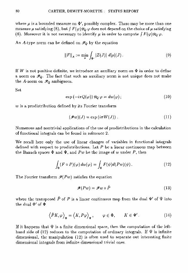
80 CARTIER, DEWITT-MORETTE : STATUS REPORT
where fi is a bounded measure on $ ' , possibly complex. There may be more than onemeasure fx satisfying (8), but / F(<p)@Q <p does not depend on the choice of fx satisfying(8). Moreover it is not necessary to identify // in order to compute / F(ip)@Q (p.
An A-type norm can be defined on &Q by the equation
\\F\\A:=mmJjZ(J)\d\n\(J). (9)
If W is not positive definite, we introduce an auxiliary norm on $ in order to definea norm on &Q. The fact that such an auxiliary norm is not unique does not makethe A-norm on &Q ambiguous.
Setexp (-i7rQ((p)) @Q(p = dw(<p); (10)
to is a prodistribution defined by its Fourier transform
(&w)(J) = exp(iirW(J)) . (11)
Numerous and nontrivial applications of the use of prodistributions in the calculationof functional integrals can be found in reference 2.
We recall here only the use of linear changes of variables in functional integralsdefined with respect to prodistributions. Let P be a linear continuous map betweenthe Banach spaces $ and \I>, and Pw be the image of w under P, then
/ (F o P)(<p) dw{v) = i F(1>)d(Pw)(il>). (12)
The Fourier transform &(Pw) satisfies the equation
P (13)
where the transposed P of P is a linear continuous map from the dual $ ' of $ intothe dual $ ' of $
(PK, <p\ = (K, PV)^ , V e *, K G * ' . (14)
If it happens that ^ is a finite dimensional space, then the computation of the left-hand side of (12) reduces to the computation of ordinary integrals. If $ is infinitedimensional, the manipulation (12) is often used to separate out interesting finitedimensional integrals from infinite dimensional trivial ones.

CARTIER, DEWITT-MORETTE : STATUS REPORT 81
2, ^e,z Integrators Satisfying (4)
Equations (8) and (9) can be generalized:
• The space &®,z of complex valued functional F o n $ , such that (8) is satisfied,is a space of functional integrable with respect to @Q,Z-
• The A-type norm defined by (9) makes it possible to state a Fubini theorem foriterated integrations.
If it happens that \i which satisfies (8) is explicitly known, then
= / Z(J)dp(J) (15)
the right-hand side being an integral in the traditional sense.
Work on constructing an axiomatic basis for functional integration with respect tointegrators satisfying (4) is in progress.
3* Quantum Field Theory Integrators
In Quantum Field Theory, the situation is different. Let
) (16)
where S is the bare action, ip is a self interacting field, or a collection of interactingfields, and J is an external source; the generating functional Z(J) cannot be chosena priori because it is an experimental quantity in the following sense. Let
expiW(J) :=Z(J)/Z(0) (17)
and let T ((p) be the Legendre transform of W
T(<p):=W(J)-n(J,<p), < ^ ^ 7
then T [(p) is the effective action which can be used to compute observable quanti-ties. We cannot use (4) to identify @®rf explicitly in Quantum Field Theory butwe shall use (4) to impose the following conditions on @e,z] they are chosen so asto make integration by parts and linear change of variable of integration straightfor-ward manipulations: namely the infinitesimal version of the invariance of 0® undertranslation
[ £ s , z < p = 0, (19)

82 CARTIER, DEWITT-MORETTE : STATUS REPORT
and the fundamental property,
if ip = M<p, t h e n Q>@,z </> = det M@e,z ¥> • (20)
The choice of functional F G ^e,z integrable by @®^z must be compatible with (19).
Given an integrator @Q,Z satisfying (19) and (20) and a map 0(9?, J) of the type (16),one can investigate a number of problems; for instance:
i) Computing /$ F(ip)exp (^S((p)j @e,z<t> for several functional F.
ii) Low energy limit of the effective action T ((p) given a bare action S(<p). Whenis the low energy limit of T ((/?, observable constants) equal to S (<£, observableconstants)?
iii) High energy limit of the effective action. When is a theory "asymptoticallyfree"?
iv) Stationary phase approximation of /$ F(ip) exp f j^S((p)) @Q,Z ¥-
In the years to come, we will write a book on functional integration and test theproposed framework on many problems of physical interest.
References
[1] Cartier P., DeWitt-Morette C , Integration Fonctionnelle; elementsd'axiomatique. To appear in the Comptes Rendus de FAcademie des Sciences.
[2] DeWitt-Morette C , Functional Integration; a multipurpose tool To appear inthe Proceedings of the International Colloquium in Honour of Yvonne Choquet-Bruhat, Eds. Flato M., Kerner R., Lichnerowicz A. Kluwer AcademicPublishers, Dordrecht. Available as an IHES reprint (IHES, 35 Routede Chartres, F-91440 Bures-sur-Yvette).

SOLUTION OF THE COUPLED EINSTEIN CONSTRAINTS
ON ASYMPTOTICALLY EUCLIDEAN MANIFOLDS
Yvonne Choquet-Bruhat
Universite Paris 6
dedicated to Dieter Brill
Abstract. We consider the coupled elliptic system of constraints on the
Cauchy data for Einstein's equations obtained by the conformal method when
the initial manifold has non constant mean extrinsic curvature r. We prove
that this system admits asymptotically euclidean solutions when Vx is small
in an appropriate norm and the scalar curvature of the conformal metric is
either everywhere non negative, or everywhere negative with fall off
conditions that we specify.
Resume. Nous considerons le systeme couple des contraintes sur les donnees
de Cauchy obtenu par la methode conforme quand la variete initiale a une
courbure extrinseque moyenne T qui n'est pas constante. Nous montrons que
ce systeme elliptique admet des solutions aymptotiquement euclidiennes
quand V T est assez petit dans une norme appropriee et que la courbure
scalaire de la metrique conforme est soit partout non negative, soit
partout negative avec un comportement a l'infini que nous explicitons.
INTRODUCTION.
An initial data set in General Relativity is a pair (g,K) , g a riemannian
metric and K a symmetric covariant 2-tensor on a 3~dimensional manifold V.
As a consequence of Einstein equations they must satisfy the constraints
(1) R _ K.K + (trK)2 = E
(2) V.K - V(trK) = J
where E, a scalar non negative function, and J, a vector field, are zero in
vacuum.
The standard procedure to solve the constraints is the use of the
conformal method inaugurated by Lichnerowicz, Li., and developped by
Choquet-Bruhat and York (cf. for instance the review article C.B-Yo). The
constraints are found to decouple into a linear elliptic system for a
vector field on V and a non linear elliptic equation, called the
83
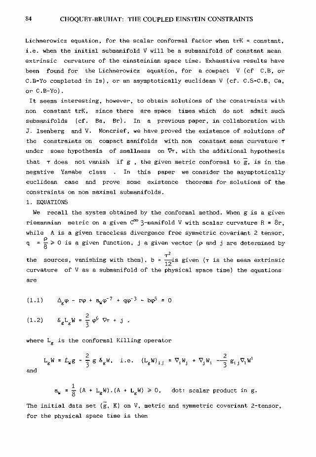
84 CHOQUET-BRUHAT: THE COUPLED EINSTEIN CONSTRAINTS
Lichnerowicz equation, for the scalar conformal factor when trK = constant,
i.e. when the initial submanifold V will be a submanifold of constant mean
extrinsic curvature of the einsteinian space time. Exhaustive results have
been found for the Lichnerowicz equation, for a compact V (cf C.B, or
C.B-Yo completed in Is), or an asymptotically euclidean V (cf. C.S-C.B, Ca,
or C.B-Yo).
It seems interesting, however, to obtain solutions of the constraints with
non constant trK, since there are space times which do not admit such
submanifolds (cf. Ba, Br). In a previous paper, in collaboration with
J. Isenberg and V. Moncrief, we have proved the existence of solutions of
the constraints on compact manifolds with non constant mean curvature T
under some hypothesis of smallness on VT, with the additional hypothesis
that T does not vanish if g , the given metric conformal to g, is in the
negative Yamabe class . In this paper we consider the asymptotically
euclidean case and prove some existence theorems for solutions of the
constraints on non maximal submanifolds.
1. EQUATIONS
We recall the system obtained by the conformal method. When g is a given
riemannian metric on a given C°° 3~manifold V with scalar curvature R = 8r,
while A is a given traceless divergence free symmetric covariant 2 tensor,p
q = -T- > 0 is a given function, j a given vector (p and j are determined byo
T2
the sources, vanishing with them), b = — i s given (T is the mean extrinsic
curvature of V as a submanifold of the physical space time) the equations
are
( 1 . 1 ) Ag<p - r<p + aw<p"7 + q<p~3 - bcp5 = 0
( 1 . 2 ) SgLgW = - c p 6 VT + j .
where Lg is the conformal Killing operator
- | g 6gW, i.e.
and
aw = — (A + LgW) . (A + LgW) > 0, dot: scalar product in g.
The initial data set (g, K) on V, metric and symmetric covariant 2-tensor,
for the physical space time is then

CHOQUET-BRUHAT: THE COUPLED EINSTEIN CONSTRAINTS 85
g = <p4g, K = <p"2(A + LgW) + i g r .
2. ASYMPTOTICALLY EUCLIDEAN MANIFOLDS. WEIGHTED SOBOLEV SPACES.
A C°° , n-dimensional, riemannian manifold (V,e) is called euclidean at
infinity if there exists a compact subset K of V such that V - K is the
disjoint union of a finite number of open sets Ui , and (\Ji ,e) is isometric
to the exterior of a ball of IF with its canonical euclidean metric.
The weighted Sobolev space W P > 5 , 1 < p < o o , S 6 [ N + , S e [ R , i s the
closure of C ° (C°° functions with compact support in V) in the norm
IDmulp
0<m<s~ V
D and I I denote the covariant derivative and the norm in the metric e,
while cr = (1 + d 2 ) ^, d the distance in the metric e from a point of V to a
fixed point; if (V,e) is the euclidean space one can choose d = r, the
euclidean distance to the origin.
We recall the multiplication and imbedding properties (cf. CB-Ch)
W s ^ S ^ W s 2 , S 2C W s , 8 i f S > S l f S 2 , S < S l + S 2 - - , & < & ± + & 2 + ^ .
w s , 8 c c l i f m < s - - , p < & + - , Hull m= 2 S u p ( I D ^ u l o J 3 + m ) .
We a l s o h a v e
3. LERAY SCHAUDER THEORY. THEOREMS ON ELLIPTIC SYSTEMS.
To solve the non linear system (1.1), (1.2) we shall use the
Leray-Schauder theory: a solution will be a fixed point, in a bounded open
subset Q of some Banach space K, of a compact mapping °F: Q -* K . The
existence of a fixed point is proved by constructing a continuous family of
compact maps !F t, t 6 [0,1], such that 3^ = 3R" and that Wo has one and only
one fixed point in ft (then Id - J 0 has degree ±1 in ft) and no Jt has a
fixed point on the boundary dQ of Q (then all the maps Wt have the same
degree in Q) .
Before defining the mappings W and !Ft we recall the following theorems.
Theorem 1. (CB-Ch,Ca). Let g be a riemannian metric on V3 with g - e E r, p

86 CHOQUET-BRUHAT: THE COUPLED EINSTEIN CONSTRAINTS
3 3and let a E W j ? 9 , a > 2 + — , < p , and a > 0. Then the equation
cr-2,P + 2 p p
3 1(3.1) Agu - au = f, with f E WP_2> 8 + 2 given, < S < 1 and & < p
has one and only one solution u £ Wj 5 .
The solution of (3«1) satisfies the inequalities
(3.2) Hull < C Hfll , s =2, ..., a .Ws,S Ws-2,S+2
where the Cfs are constants depending only on V, e, g, a.
Theorem 2. Let g be a riemannian metric on (V^,e) such that g - e E W^ p,
3 3a > 3 + — • p > - — , then (V,g) admits no conformal Killing vector field
P Pand the system
(3-3) &gLgW = h, with h E WP. _ 2 f 8 + 2 given,
3 32 < a1 < cr , - - < & < 1 - - and S < p
P P
has one and only one solution W E Wg., 8 . It satisfies the inequalities
(3.4) HWII < C Hhll , s = 2,...,cr» .Ws,3 Ws-2,8+2
Proof. The non existence of a conformal Killing vector field is
proven in Ch-OM. For existence of W and inequalities, cf CB-Ch. and Ca.
Definition. We say in the following that the data g, A, q, j, T on (V, e)
a r e p - p - r e g u l a r l y a s y m p t o t i c a l l y e u c l i d e a n i f g - e E W g - p , c r > 3 + — ,
3 P
A G W 2 , P + I » ^' J G W I ,P+2 a n d T E W 2 ,P + I • w i t h P + - > 0. It results that
T 2
R G WP.2>p + 2, while A.A , b = — E W?fP + 1.
4. CASE R > 0.
The construction of the compact maps Wt , choice of Q and proof of non
existence of fixed points on dQ will be different depending on the sign of
R. We first consider the case R > 0 on V.
Let there be given a function ij; E 1 + v and a vector field to on V. We
consider the linear system of differential equations depending on a real
parameter t, with unknown <p and W:

CHOQUET-BRUHAT: THE COUPLED EINSTEIN CONSTRAINTS 87
( 4 . 1 ) Ag<p - r<p =
i . e . Agu - ru = r + tf(v,co) , u = <p - 1
with f (v,w) = awi|/~7 + q\|/~3 - b\\P , \\x = 1 + v
and aw = - (A + L co) . (A + L co) ,o s 6
( 4 . 2 ) &gLgW = - t ^ 6 Vr + j .
Lemma 1. Let g, A, q, j, T be p-p-regularly asymptotically euclidean on
(V,e) with p > 3 .
Let H be the Banach space of pairs (v , CJ) such that v G W{ 5, co 6 WP, s •
Let fi be the bounded open subset of H defined by the inequalities
(4.3) Hvll _ < k,W1.S
(4.4) Ikoll n < k1,
where k and kf are some given positive numbers, and
(4.5) Inf(1 + v) > & > 0V
with & some number such that 0 < £ < 1.
Then, if < & < 1 - — , & < p the resolution of the linear systemP P
(4.2) on V^ defines for each t E |R a compact map !Ft :
Jt : Q -> H by (v = i|/-l, id) » (u = <p-l, W),
Proof. Q is open in H because on (V,e) we have the continuous inclusion3 3
W§ 5 c C^, space of continuous and bounded functions, if 1 > — , 8 > - —.
We recall that W*J, 5, c W^ 8 if s' > s and 6f > &, with compact imbedding
if both inequalities are strict.
Imbedding and multiplication properties of W^ 8 spaces show that under the
hypothesis made

88 CHOQUET-BRUHAT: THE COUPLED EINSTEIN CONSTRAINTS
i f & < &f < & + ( & + - ) .P
On the other hand v E Wp1 5 with 1 + v > t > 0 implies that (l+v)N is
continuous and uniformly bounded on V-. for any positive or negative-* 3
integer N, while V(l+v)N E Wp0 s + 1, from which results since & + — > 0 that
f £ W ^ s«+2 if*we impose moreover
Analogous considerations show that h E Wp1 s.+2*
The linear system (4.1), (4.2) has therefore one and only one solution
(u, W) which is not only in W^ s*Wp2 8 b u t a l s o i n w?3 8«xWP3 5« » therefore
the mapping 3F~t: (v,co) *-> (u,v) is a compact mapping from Q into H.
Lemma 2_ Let g, A, q, j, T be p-p regularly asymptotically euclidean, with
R = 8r > 0 Suppose p > 3• Denote by S and &f numbers such that
P PThen
1) The s o l u t i o n <p0 = 1 + u0 , u0 E Wp p c Wp3 § 5 , of
( 4 . 6 ) Ag<p0 - rcp0 = 0
is such that there exists a number a > 0 and so that on V
0 < a < <p0 < 1 .
2) Let there be given b0 > 0 ,b0 E Wp1 > 5,+ 2 . The equation
(4.7) Ag*0 - r*0 - b 0 ^ = 0
admits a solution <f>0 = 1 + Uo , UQ E W^ 8, c W^ s. This solution is unique
and there exists t > 0 such that
<p0 on
3) Suppose a1 E Wp , ax > 0 , be given. The equation1 , 8 ' + 2
(4.8) Ag *x - r^ + a^"7 + q4»"3 = 0

CHOQUET-BRUHAT: THE COUPLED EINSTEIN CONSTRAINTS 89
admits a solution <£., such that <k = 1+lL , tL E Wp . This solution is3,5 + 2
unique and satisfies
<P0 < *i •
4) If ax > aw and b 0 > b , then any solution <p > 0, with cp - 1 E W p3 > 8 , of
Ag<p - r<p = - t f s^cp ' 7 + qcp"3 - bcp5)
i s such t h a t
(4 .9 ) * 0 < <p< * ! .
Proof, It makes repeated use of the maximum principle: if <p E C2 satisfies
the linear inequality on V
Agcp - h <p > 0 , with h > 0 and bounded
then <p cannot attain a non negative maximum M except if <p = M.
1) Since <p0 is C2 and satisfies (4.6) it is constant if it attains a non
negative maximum. Since <p tends to 1 at infinity on V^ it attains such a
maximum on V^ if it takes values greater than 1, hence <p0 < 1. An analogous
reasonning applied to - <p0 shows that <p0 cannot attain a non positive
minimum.
2) We solve (4.7) by using the Leray-Schauder theory. We consider the
compact mappings Ft: Wp 1 8 -* Wp^ s, c Wp
1 s by v *-> u obtained by resolution
of the linear equation
A $ -r4> = t
in the bounded open s e t Q
llvll < k , k > 0 some given number,W i , 8
Sup 4 > < l + € , € > 0 some given numberxEV
The mapping FQ has one fixed point in , u0 = <p0 - 1, if k is chosen such

90 CHOQUET-BRUHAT: THE COUPLED EINSTEIN CONSTRAINTS
t h a t k > llunll n
° W ? , 8All mappings F t are such that if v E Q then Hull < Hull < K where K
Wl , 8 W 2,8
depends only on € and on the Wp0 > 5 norms of r and b0 .
The maximum principle shows on the other hand that a fixed point <$> of
F t in Q cannot take non positive values, i.e. $ > 0 on V^ , because <£ tends
to 1 at infinity and satisfies the linear equation
Ag4> - ( r + tbo$4)<J> = 0 .
The inequality <P < <p0 is then a consequence of the equation
A g (* - <p0) - r(* - <p0) = t bo*5
and the fact that <P - <p0 tends to zero at infinity.
These results show that we can choose k and take € > 0 arbitrary such that
no yt has a fixed point on dQ, intersection of Q with one or the other of
the two sets
Hull = k and Sup<J> = l+€ .W1,S V
We denote by <f>0 the solution of the original equation (4.7) and by 2t its
strictly positive infimum on V^. The uniqueness of this positive solution
is again a consequence of the maximum principle.
3) The equation for <t>x is the usual Lichnerowicz equation on maximal V,
the existence and uniqueness of ^ > <p0 is well known (cf. CB.Yo)
4) A solution q> > 0 of the equation
Ag<p -r <p = -t(aw<p"7 + q<p'3 -bcp5)
satisfies the linear equation
V < V < p ) " {r+bt(^+^<p+...+(p4)}(^o-<p) = <&o (bo-tb)+t(aw(p"7+qcp"3) >0 .
from which we deduce since <p > 0 and <P0 - <p tends to zero at infinity that
$0 - <p < 0 on V^ .

CHOQUET-BRUHAT: THE COUPLED EINSTEIN CONSTRAINTS 91
A similar proof shows that
<p - 4^ < 0 on V^ .
We now prove an existence theorem for the coupled system.
Theorem. Let g, A, q, j, r satisfy the hypothesis of lemma 2. There exists
a number rj > 0 such that if IIVTII < TI for some & with - — < S < 1 - —W0,S+2 P P
the constraints admit a regularly asymptotically euclidean solution on V.
Proof.
Let Q be the bounded open s e t of Wx §xW2 § defined by
(4.10) Ikp - 111 n < k , HWII n < kf ,
(4.11) Inf (<p - *0) > - t , Inf ( - <p) > - IV V
where <J>0 is the solution of an equation (4.7) with b0 > b , hence <P0 is
known from the data, while 4^ = 1 + ux, ut G W^ s is solution of the
following equation, where M is some positive number to be chosen laterM
(note that by a result quoted in §2 we have E W^ § + 2)
= 0,
w i t h (3 some number such t h a t
& + - < 3 < & f + - .P P
The supremum of *P^ on V^ is some increasing function of M, jx(M) . We denote
m(M) = \x(yi) + t . We have for <p E ft
q> < m(M) on V^ .
A fixed point will not lie in the boundary dQ if it satisfies the strict
inequalities (4.10), (4.11).
A fixed point (u, W) of Wt satisfies the inequalities
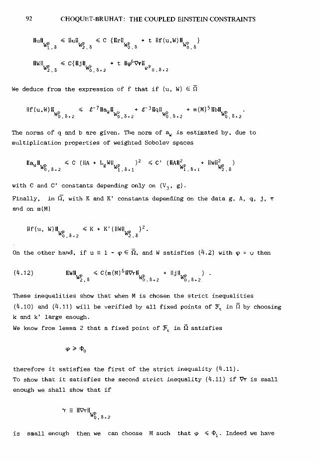
92 CHOQUET-BRUHAT: THE COUPLED EINSTEIN CONSTRAINTS
We deduce from the expression of f that if (u, W) E Q
llf(u,W)ll < t-^WLP + ^ 3 W I p + m(M)5||bllw 0 ,S+2 w 0 , 8 + 2 w 0 , 8 + 2 w 0,S+2
The norms of q and b are given. The norm of a^ is estimated by, due to
multiplication properties of weighted Sobolev spaces
with C and Cf constants depending only on (V , g).
Finally, in Qf with K and K* constants depending on the data g, A, q, j, T
and on m(M)
llf(u, W) II < K + K'(HWII ) 2 .W0,8+2 W2,8
On t h e o t h e r hand , i f u = 1 - <p G ft, and W s a t i s f i e s ( 4 . 2 ) w i t h <p = \|/ t h e n
( 4 . 1 2 ) HWII < C(m(M)6IIVTll + lljll ) .W 2 , 8 W 0 , 8 + 2 W 0 , 8 + 2
These inequalities show that when M is chosen the strict inequalities
(4.10) and (4.11) will be verified by all fixed points of Wt in Q by choosing
k and kf large enough.
We know from lemma 2 that a fixed point of yt in ft satisfies
<P > %
therefore it satisfies the first of the strict inequality (4.11).
To show that it satisfies the second strict inequality (4.11) if VT is small
enough we shall show that if
is small enough then we can choose M such that <p < 4^ . Indeed we have

CHOQUET-BRUHAT: THE COUPLED EINSTEIN CONSTRAINTS 93
proved in lemma 2 that this inequality holds if
( 4 . 1 3 ) aw < — — , i . e . HaJI 0 < M
By inclusion properties of weighted Sobolev spaces we have
P . since
3We know that if &' < S + (S + —) we have
P
Therefore if (1 - <p,W) E ft we see, using the inequality (4.12), that (4.13)
is satisfied if
m(M)12IIVrll2 + | | j | |2 + HAII2 < C M .
W 0 , S + 2 W 0 , S + 2 W 1 , S + 1
i.e. T 2 < m ( M ) " 1 2 { C M - ( l l j l l 2 + IIAII2 }W 0 , 8 + 2 W 1 ? S + 1
We choose M such that the number between parenthesis is stictly positive,
and then y > 0 small enough to satisfy the above inequality.
We have proved that no mapping !Ft: Q -• K , t E [0,1] has a fixed point on
dto.To complete the proof it is sufficient to show that yo has one fixed
point in Q. Since !F0 is the constant map (v,co) »-> (uo,Wo) it wil be the case
if k and kf are chosen such that (uo,Wo) satisfy the inequalities (4.10),
because we already know that <p0 satisfy (4.11).
5. CASE R < 0.
When R = 8r < 0 the mappings Jt: (v,co) •-• (u,W) will be defined
by resolution of the linear system
( 5 . 1 ) A g u = t f ( v , c o ) , f ( v , c o ) E n ] / - a^ i i / " 7 - qi|r"3+ b\\f5 , i[/ = 1 + v
( 5 . 2 ) 8 g L g W = | i i r 6 y r + j
w i t h (v ,0) ) E n , a n o p e n b o u n d e d s u b s e t o f t h e s p a c e H o f lemma 2 i n § 4 .
S i n c e t h e o p e r a t o r rep - a<p" 7 - q<p"3 + bep5, a > 0 , q > 0 , b > 0 , i s n o

94 CHOQUET-BRUHAT: THE COUPLED EINSTEIN CONSTRAINTS
longer monotonic in <p another version of the maximum principle has to
be used to prove that no 3^ has a fixed point on 3ft, namely:
If u E C2 , it cannot attain a maximum at a point x where (Agu)(x) > 0
[resp., a minimum at a point where (Agu)(x) < 0.]
Theorem. Let g,A,q,j,r be p-p regularly asymptotically euclidean, p > 3»
Sup
(5.
(5.
POS(
3)
•0
* R = 8r <: 0 and
Inf (bV
InfV
(recall
Irl— = x
T2
b = —12
= B > 0
> 0 ,
Then there exists TJ > 0 such that the system (1.1), (1.2) has a solution
( < p > 0 , W ) w i t h l - < p , W E W P 8 , - - < & < I n f ( p , l - - ) i f I I V T I I n < r |J' P P W O , P + 2
and (3 is such that & + - < ( 3 < & f + - with & < &' < Inf (p,l ) .P P P
Proof. The mappings 3Ft are now the family of compact maps defined by
resolution of the linear system (5.1), (5*2) in the closure of the bounded
open set ft c H defined by the inequalities (4.10) and
(5.4) Inf <p > t , Sup < p < m , <p=l + uV V
where t and m are numbers to be chosen later and are such that
(5-5) 0 < I < 1 < m .
The mapping !F0 : (v,to) •-+ (0,W0) has one fixed point in Q if kf is large
enough for the second inequality (4.10) to be satisfied by Wo.
All mappings Wt : Q -* K will have a range satisfying the strict inequalities
(4.10) if k > K, kf > K f where K and K1 are numbers depending on the data
and on £, m .
To show that a fixed point of !Ft satisfies the strict inequalities (5*4) we
start in the usual way, used also in CB-Is-Mo in the case of a compact V^,
namely we consider the polynomial
P(z) E bz3 - Irlz2 - qz - a^
A fixed point <p = 1 + u of 3<t, t E (0,1], in Q satisfies

CHOQUET-BRUHAT: THE COUPLED EINSTEIN CONSTRAINTS 95
Ag<p = t <p"7P(z) , tk < z = <p4 < m4 .
To show that <p satisfies the strict inequalities (5*4) it is sufficient to
show that at a maximum where cp = m [resp. at a minimum where cp = t~\ we have
P(m4) > 0 , [resp. P(£4) < 0 ] .
Since q > 0, aw > 0 we shall have P(£4) < 0 a fortiori if
Irlt > 0 and £ < A = Inf .
V b
On the other hand we shall have P(m4) > 0 if m4 > n(A,B) with [x(A,B) the
positive root of the equation
Bp,3 - pix2 - Q|x - M = 0
with p > llrll 0 , Q > llqll 0 ,GT+2 CT+2
(5.6) M > llajl 0 .C|3+2
Numbers B > 0, p > 0 and Q > 0 depending only on the data exist by the
hypothesis made on these data and on (3. A number M exists for each fixed
point of a mapping !Ft because then W E W^ §, .
The following choice of & and m satisfy the requirements
(5-7) 0 < t < Inf (A,l), m > Sup(M,(M,B)1/4,l),
We have only to check, as in §4, that, for a fixed point of Jt in Q, aw
satisfies (5.6). We are led to an inequality of the same form as (4.13)
with now m(M) given by the inequality (5*7)• The size of y can be estimated
as in CB-Is-Mo.
REFERENCES
[Ba] R. Bartnik "Remarks on constant mean curvature surfaces in
cosmological space times", Comm. Math. Phys. 117 p.615-624, 1988.

96 CHOQUET-BRUHAT: THE COUPLED EINSTEIN CONSTRAINTS
[Br] D. Brill "On space-times without maximal surfaces" in Proceedings of
the third Marcel Grossmann meeting, Beijing 1982 H Ning ed. North Holland
1983.
[Ca] M. Cantor "The existence of asymptotically flat initial data for
vacuum space- times" Comm. Math. Phys. 57 P-83-96, 1977-
[C.S-C.B] A. Chaljub-Simon and Y. Choquet-Bruhat "solution of the problem
of constraints on open and closed manifolds" Jour. Gen. Rel. and Grav. 5
p.47- 64, 1974.
[C.B] Y. Choquet-Bruhat "Global solution of the problem of constraints on a
closed manifold"
Acta di Istituto di Alta Matematica, Rome, 12 p.317-325, 1973
[C.B-Ch] "Elliptic systems in Hs 8 spaces" Acta Matematica 146 pl29-150t
1981.
[C.B-Yo] Y. Choquet-Bruhat and J. York "The Cauchy problem" in "General
Relativity", A. Held ed. Plenum 1979.
[C.B-Is-Mo] Y. Choquet-Bruhat, J. Isenberg and V. Moncrief "Solution of
constraints for Einstein equations" C.R. Ac. Scie. Paris, to appear 1992.
[Ch-OM] D. Christodoulou and N. O'Murchada "The boost problem in General
Relativity" Comm. in Math. Phys. 80 p271-300, I98I.
[Is] "Parametrization of the space of solutions to Einstein equations"
Phys. Rev. letters 59 p2389~2392, 1987.
[Li] A. Lichnerowicz "Sur 1fintegration des equations d'Einstein" J.Math.
Pures et Ap. 23 p.37-63, 1944.

Compact Cauchy Horizons and CauchySurfaces
P. T. Chrusciel * J. Isenberg t
Abstract
We show that if a globally hyperbolic spacetime (M,#) extends to a nonglobally hyperbolic spacetime (M', #'), and if the Cauchy horizon Ji for M inM' is compact, then the Cauchy surfaces for (M,g) must be diffeomorphic toTi. As a corollary to this result, we show that if a (2 + l)-dimensional spacetimehas compact Cauchy surfaces with topology other than T2, then it cannot beextended to a spacetime with a compact Cauchy horizon.
1. Introduction
Dieter Brill and one of us (JI) used to talk a lot about Mach's Principle. We both wereof the Wheeler school, so our Machian discussions often focussed on issues involvingthe initial value formulation of Einstein's theory. One such issue was the followingquestion: If a spacetime (M,#) is known to be globally hyperbolic, how can onetell (from intrinsic information) if a given embedded spacelike hypersurface £ is aCauchy surface for (M,#)? The answer to this question is important if one wantsto know what minimal information about the universe "now" is needed to determinethe spacetime metric (and hence its inertial frames) for all time in (M,g).
It turns out [1] that if a spacelike hypersurface S embedded in a globally hyperbolicspacetime is compact (without boundary), then it must be a Cauchy surface. So,whatever the topology of S, all Cauchy surfaces in (M,g) must be diffeomorphicallyequivalent to S; and indeed it follows [2] that M must be diffeomorphic to £ X 3£.
* Alexander von Humboldt fellow, on leave of absence from the Institute of Mathematics ofthe Polish Academy of Sciences. Max-Planck-Institut fiir Astrophysik, Karl Schwarzschild Str. 1,D8046 Garching bei Munich, Germany. This author was partially supported by the National ScienceFoundation under grant # PHY-902301 at the University of Oregon and by a KBN grant # 2 10479101. e-mail: [email protected].
t Department of Mathematics and Institute for Theoretical Science University of Oregon, Eugene,OR 97403, USA. This author was partially supported by the National Science Foundation undergrant # PHY-902301 at the University of Oregon.
97
98 CHRUSCIEL & ISENBERG : COMPACT CAUCHY HORIZONS
Let us say we consider a spacetime (M\gf) which is not globally hyperbolic; however,in (M\g') there is a globally hyperbolic region (M,g) with the boundary of M in M1
forming a Cauchy horizon 7i, Is there any necessary topological relationship betweenthe Cauchy horizon 7i and the Cauchy surfaces in (M,#)? In this paper, we show(Theorem 3.1) that if 7i is compact (without boundary) then the Cauchy surfaces in(M,g) must be diffeomorphic to 7Y, and hence M = 7i x 3ft.
It follows from this result that a spacetime which is generated from initial dataspecified on a noncompact Cauchy surface cannot be extended across a compactCauchy horizon. If we consider (2 + l)-dimensional spacetimes, Theorem 3.1 evenlimits the class of spacetimes with compact Cauchy surfaces which may be extendedacross a compact Cauchy horizon. We recall [3] the fact that a Cauchy horizon isnecessarily ruled by a congruence of null geodesies. It follows by a simple argumentthat H admits a nowhere vanishing vector field. But the only compact (orientable)two-dimensional manifold which admits a nonvanishing vector field is the two-torus,T2. Hence, if a (2+1) dimensional globally hyperbolic spacetime has Cauchy surfaceswhich are not two-tori, then it cannot be extended across a compact Cauchy horizon(Theorem 4.2).
Theorem 4.2 is relevant to a question which arose among a number of us (Brill, Eard-ley, Horowitz, Moncrief, and the two authors) at Aspen in 1990. Recall the Misner( l+l)-dimensional , flat cylinder, spacetimes [4]. Often used to model the behav-ior of Taub-NUT spacetimes, these Misner spacetimes extend across a compact (S1)Cauchy horizon. Besides these standard (l-fl)-dimensional Misner spacetimes, thereare (2 + 1), (3 + 1), and indeed (n + 1) (any n) dimensional versions of them. Some ofthe generalized Misner spacetimes are obtained simply by taking the direct productof a (1 + 1)-Misner spacetime with a flat (n — l ) - torus . Their Cauchy surfaces aren-dimensional tori, and they extend across compact Cauchy horizons (also T n ' s ) . Butthere are other, more perplexing (n + l)-dimensional generalized Misner spacetimeswhich are obtained by taking the interior of the future light cone through a point in(n + 1 )-dimensional Minkowski spacetime, and then quotienting by the action of acertain discrete subgroup of the Lorentz group so as to spatially identify the space-times. For appropriate subgroups of the Lorentz group the resulting space-time willbe spatially compact. The Lorentz subgroup action which is quotiented out preservesthe constant mean curvature ("mass hyperboloid") hypersurfaces in the interior of thefuture causal cone; so these negatively-curved hypersurfaces serve as Cauchy surfacesfor the resulting spacetimes. Can these generalized Misner spacetimes be extendedacross a Cauchy horizon?
Noting that the spacetimes are flat, and geodesically incomplete, one might expectthat a Taub-NUT-like (and Misner-like) extension can be carried out. However, atleast in the (2+l)-dimensional case, it follows from our results that if an extensioncan be made, then the resulting Cauchy horizon must be noncompact. For if the

CHRUSCIEL k ISENBERG : COMPACT CAUCHY HORIZONS 99
Cauchy horizon were compact, it and therefore the Cauchy surfaces would have tobe two-tori. But the compact "mass hyperboloid" Cauchy surfaces have constantnegative curvature, so they must be two-manifolds of genus greater than or equal totwo. It remains to be seen if one can extend these Misner spacetimes across a noncompact Cauchy horizon of some sort.
This paper is primarily devoted to proving Theorem 3.1. In preparation for doingthis, we discuss definitions and conventions, and recall some properties of globallyhyperbolic spacetimes in Section 2. The statement and proof of Theorem 3.1 appearsin Section 3. Then in Section 4. we discuss its corollaries (including Theorem 4.2)and make some concluding remarks.
2. Preliminaries
We work here with spacetimes which are Ck Lorentz manifolds (M,g) for k > 3.Generally we assume that M is a Ck, paracompact, HausdorfF, connected, (n + 1)-dimensional manifold (n > 1), and that g is a Ck~x Lorentz-signature metric onM.
At any point p G M, the metric g divides the set of tangent vectors V G TPMinto subsets which are timelike (if g(V, V) < 0), spacelike (if g(V, V) > 0), or null (ifg(V, V) = 0). The timelike vectors in TPM split into two disconnected families, whichone can arbitrarily label "future timelike" and "past timelike." These designationshave nonlocal meaning iff the spacetime is time-orientable. By definition, a spacetimeis time-orientable iff for any continuous map T : S1 —> M of the circle S1 into thespacetime manifold M, and for any choice of (i) a point p0 = T(0O) in the imageof the map and (ii) a timelike vector Vo G TPoM, there exists a continuous mapf : S1 -> TM such that f(0) G TT(e)M, and f(0o) = %, with f(0) timelike (non-vanishing) for all 6. So if a spacetime is time-orientable, there is a continuous globaldistinction between future timelike and past timelike vectors. One easily verifies thatif (M,g) is time-orientable, there exists a Ch~x vector field X on M which is timelikeeverywhere (and either future timelike or past timelike everywhere). Note that, bydefinition, such a vector field is nowhere vanishing.
Time orientability is a mild restriction on a spacetime (M,</); indeed, if (M,g) isnot time orientable, it always has a double cover which is. The condition of globalhyperbolicity, on the other hand, is quite strong. If (M,g) is globally hyperbolic,then all of the following must be true [2, 3]:
a) (M, g) must be time orientable.
b) There exists a Ck embedded Cauchy surface in (M,</); i.e., there exists an n-dimensional hypersurface S embedded in M such that every inextendible causal

100 CHRUSCIEL k ISENBERG : COMPACT CAUCHY HORIZONS
path in M intersects S once and only once.
c) There exists a Ck function T : M —» $£ with nowhere vanishing gradient such thatthe level sets of T are all Cauchy surfaces £ y in (M, #). This "time function"can be chosen so that its image includes all of the reals, and then it followsthat for any future-directed inextendible causal path 7 : 3? —» M , one has
oo T o 7(5) = +00 and Iim5_>_oo T o 7(3) = —00.
d ) Any pair of Cm Cauchy surfaces in (M,g) for 0 < m < fc, are Cm diffeomorphic.
It is an immediate consequence of these properties of globally hyperbolic spacetimesthat every Cauchy surface is a closed subset of (M, g) and M is Ck diffeomorphic to£ X / , where / is an interval (possibly infinite) in 3£. Further, one readily verifies thatif one does not assume a priori that M is connected, then — assuming that (M,g) isglobally hyperbolic — M is connected iff its Cauchy surfaces S are connected.
In this paper, we are interested in globally hyperbolic spacetimes (M, g) which can beextended past their domains of dependence to some non globally hyperbolic spacetime(M\gf). In particular, we are interested in studying the boundary of dM of M inM' , which is called the Cauchy horizon of M.
Let us recall the topological nature of the boundary dA of any set A in B. If wepresume that A is open in B (as we shall for M in M' ) , then by definition dA consistsof all those points p G B \ A for which there exists a sequence pi which lives in Aand converges to p. The boundary dA inherits a natural topology from B: a subsetO of dA is open in dA iff there exists an open subset U of B such that O = dA D U.It follows that if C C dA is a connected component of dA, then there exists an openset of U C B such that U PI dA = C. This fact plays a role in the proof of Theorem3.1, below.
Before we state and prove our main result, we wish to establish a technical resultconcerning flows on spacetime. Let </>s{p) denote the flow of a vector field X , asdefined by the differential equation j;<t>s{p) = X o (j)s(p). We shall need the following.
L e m m a 2.1 Let Q be a compact subset of a Ck spacetime (M,g) (with k > 2) andlet U be an open neighborhood of Q. Let X be a C£ vector field on M} with £ > 1.There exists So > 0 such that for all s G [—«s 0, + so], one has <f>s(Q) C U.
Proof : Since M is Hausdorff and paracompact, there exists a Ck~x Riemannianmetric h on M such that (1) (M, h) is a complete Riemannian manifold, and (2) themetric topology induced on M by the distance function dh associated to h coincideswith the original topology on M [5].

CHRUSCIEL k ISENBERG : COMPACT CAUCHY HORIZONS 101
Now, for each point p G Q, there exists a positive number rp such that the metricballs J3(p, 3rp) := {q G M \ dh(p,q) < Srp} are open, have compact closure, andare contained in U. Since Q is compact, the covering {J3(p, rp)}p€Q of Q has a finitesubcover {#(p;,rp.)};G[lj2...,i]. K w e n o w choose d0 := mint€j{rp.} and define the set
K := {m e M \dh(m,Q) <d0}
then we find that K C U. To see this, we calculate
dh(m,pi) < dh(m,p) + dh(p,pi) for any point p G £ ( # , rPi)< do + rPi
< 2rp. ,
and recall that B(p,3rpi) C C/ for all i G / . Note that since K C Uf=1JB(pt-,3rpt-), Kis compact.
Consider the function
where || X(p) \\h is the norm of the vector X(p) with respect to the inner product hat p. Since X is C^ and h is C*"1, / is a continuous function on K. Thus, since Kis compact, we have
Co :=sup/ (p) < oo
Now, for each p G Q, consider the flow path <f>s(p). If we choose £ so that <j>s{p)remains in K for all s G [0,tf], then the length L(t) of the path <f>s(p) for 5 G [0,t]satisfies the inequality
= f\\x{<j>a{P))\\hds<cot.Jo
Hence, if we choose |^| < do/Co we shall have dh(<j>t{p), Q) < d0, so <j>t(p) G J7 for allpe Q. •
3. Main Result
We now state and prove our main result.
Theorem 3.1 Let (Mf,g') be a Ck (with k > 3), (n+l)-dimensional, time orientablespacetime. Let (M,g) with g = g'\M, be a globally hyperbolic spacetime open inMf. If there exists a connected component H, of dM which is a Cl (with 1 < £ <k — 2) compact^ submanifold of Mf, then every Cl Cauchy surface S in (M,g) is Cl
diffeomorphic to 7Y.

102 CHRUSCIEL k ISENBERG : COMPACT CAUCHY HORIZONS
Remark: It should be noted that the result above is somewhat more general thanthe case in which Ti is a Cauchy horizon: Indeed, the result holds for M's which donot necessarily coincide with the interior of £)(E;M'), where D(Y,;Mf) denotes thedomain of dependence of the hypersurface S in M'. In fact, it even holds when thehypersurface £ above is not achronal as a subset of M'.
Proof : The basic idea of the proof is to use a timelike vector field in M' to dragH diffeomorphically into the globally hyperbolic region M, and then show that thedragged 7i is diffeomorphic to some Cauchy surface in M. Since the spacetime(Af ,</) is, by assumption, time orientable, there always exists a globally defined(nonvanishing) time-like vector field on M', which we shall call X. Let <f>s be the flowgenerated by X (cf. Section 2.).
Before studying the action of <>s, on W, we need to note two important properties ofTi. These properties follow from the fact that H lies in the boundary of the globallyhyperbolic spacetime (M, g), and the fact that the topology of W e dM guaranteesthat there exists a neighborhood of 7i in M1 containing no points of dM other thanthose in 7Y. Using arguments much like those in [2], we establish the following:
Lemma 3.2 Under the hypotheses of Theorem 3.1 we have:
(a) The dimension ofH is one less than that of its ambient manifold Mf.
(b) For any point p G 7i and any timelike vector V G TpMf, V is transverse to 7i(I.e., the projection of V into TpTi C TPM' does not equal V itself).
Since X is timelike and therefore everywhere transverse to 7Y, we expect either theflow (j)s — or (f)- s — to move 7i into M. Let us assume, without loss of generality,that we have chosen X so that at least for some specified point p G 7Y, <t>s(p) £ M forso < s < 0, for some so. We now verify the following:
L e m m a 3 . 3 There exists S > 0 such that for —6<s<0
( a ) <j>s{H) C M
(b) < s(W) is a compact C£ submanifold of M (where 0 < £ < k — 2, and wepresume that 7i is a Ce submanifold of Mf.)
Proof : Since X is everywhere timelike and transverse to W, and since Ji is a Cl
submanifold of M7, it follows from the properties of flows that there exists someSo > 0 such that if |s| < So, then <j>s(l~l) is a C* submanifold of M1 as well.
CHRUSCIEL & ISENBERG : COMPACT CAUCHY HORIZONS 103
Now let us define the sets
for any pairs si < 52 with |si| < so and |s2| < $0- One readily verifies (from theproperties of flows) that Kg is Cl diffeomorphic to [51,52] x H. Since H is compactand connected, it follows that Kg is compact and connected in M1.
It is useful to define on Kg the function
r-.Kg -> ftp h-> 5 such that p £ </>s(?i).
This is a well-defined function, and one verifies that it is Cl when I < k — 2.
Since H. is a connected component of the boundary of the open set M in M\ we find(as noted in Section 2.) that there exists an open set W in M' such that 7i C W, yetW fl (dM \ H) = </>. Using Lemma 2.1, we then find that for some 8 > 0, the set K6_6
is contained in W. It follows that K6_s H dM = Ti. This implies in particular that forM < S, if ^ ( W ) fl dM ^ 0, then 5 = 0.
Now let p be a point in 7i. Since 7i C 5M, it follows from the definition of topologicalboundary that there exists a sequence pi £ M which converges to p. By the definitionof convergence, there exists some i such that if i > ?, then pi £ K6_$>> and pi £ i^# .Further, we can always find a subsequence pin of pi such that (i) p^ is the firstmember of the subsequence — i.e., pi 0 = p^ (ii) pin £ i i ^ ; and (iii) rn := r(pZn) ismonotonically increasing. Possibly decreasing the value of 8, we may also guaranteethat pio £ <£_s(W).
We now consider the sequence of sets
On := /Q + 1 n M
Since pln and Pin+1 are both contained in On, the sets 0 n are non-empty. Since Mis open, On is open in / ^ + 1 . We wish to argue that On is closed in K%+1 as well.Suppose this were not true; then there must be a sequence of points qm £ On whichconverges to #00, with q^ £ K^+1 but q^ $ On. So q^ must be an element of M'\M.But if (/oo is the limit of a sequence in O C M and q^ £ M' \ M, it follows that#00 £ dM. Since #00 is supposed to be an element of K^*1 as well, this tells us thatK;**1 n dM is not empty. But K%+* C K6_s, so K^+^n dM C W. And, we notedabove that for 0 < |5| < <S, we have < S(W) fl dM — 0. So we have a contradiction; itfollows that On is closed in K%+1 •
Since Kl"*1 is connected, and since On is nonempty, open in iCJ£+1, and closed inZ^+S it follows that On = K?*1. Thus K^1 is a closed subset of M. It followsthat for all values of 5 for which rn < 5 < r n + i , one has <f>s(H) C M. Since rx = — 8and since rn+i approaches zero, in fact ^5(W) C M for all 5 satisfying — 8 < 5 < 0.

104 CHRUSCIEL k ISENBERG : COMPACT CAUCHY HORIZONS
To show that , for these values of s, ^ ( W ) is compact in Af, we use the facts (estab-lished above) that the sets K*"*1 are compact in Af, and that for r n < s < r n+i ,
is a closed subset of K^+1. This completes the proof of Lemma 3.3. •
Let us return to the proof of Theorem 3.1. We have now determined that for eachvalue of s satisfying — 6 < s < 0 (6 > 0 defined in Lemma 3.3), the set <j>s{7i) isa compact C£ submanifold of the globally hyperbolic spacetime Af. If, in addition,we knew that (f>s(7i) were spacelike, then it would follow [1] that (j)s(7i) must be acompact Cauchy surface for Af; we would be essentially done with the proof of thetheorem. However we do not know a priori that (f>s(7i) is spacelike, so there is morework to do.
Since (Af, g) is globally hyperbolic, there exists a globally defined time function T :M —> 3£, the level sets of which are Cl Cauchy surfaces in (Af,#) (cf. Section 2.).Changing time orientation if necessary we may assume that X is future oriented. Letus moreover assume that T has been chosen so that the range of T is the whole of 3£,and let us define
T+ := sup{t{p) | p e (t>
Since T is a continuous function on M and since < S(7Y) is compact in M, it followsthat T+ is finite. Thus the set
S+ := {p e M | T{p) = T+}
is a Cl Cauchy surface.
To show that S + is compact in M, we shall first show that S + fl K% is compact inAf, and then later prove that £+ H K^6 = S+. Since we know that S + , as a Cauchysurface, is a closed set in Af, it follows that if we can show that
Z+nK°_scK3 (1)
for some 0 < 7/ < £, then since KZs is compact in M, it follows that S+ fl K(i6 mustbe compact as well.
Suppose that the inclusion (1) is false. Then there must be a sequence S{ convergingto 0 and a choice of pi G < 5i(W) such that pi £ X+. These pi are contained in K0.S}
which is compact in Af' (not in Af); so there must be a point p £ 7i and a subsequenceS{n of S{ such that pin converges to p. Now consider a timelike inextendible curve Fin Af such that
Since E+ is a Cauchy surface, there exists a point q £ S + such that q = £+ fl F. Itfollows that p (to which F converges in Af') lies in the future set I*(q) of q £ £+.But the sequence pin £ £+ converges to p, so for sufficiently large n, pin must be in

CHRUSCIEL & ISENBERG : COMPACT CAUCHY HORIZONS 105
7+(</) as well. This contradicts the achronality of S+, so the inclusion (1) must hold.Hence, we conclude that S + fl K^_s = £+ fl KZ$ is compact in M.
We wish to now define a C£ diffeomorphism from (j)-$CH) — which is C* diffeomorphicto 7i — and £ + . To do this, let TT be any point in (frsCH) and define the function
We verify that GT is Cl (and hence continuous), that 0^(0) = T(TT) < T+, and thatov diverges to +oo as s approaches 8 (since the time function T diverges to +oo asone approaches the horizon). Hence, by the Intermediate Value Theorem, there issome SK for which a(s^) — T+; and therefore <j>Sir(^) £ £+ . This defines the Cl map
The map ip is injective, since the timelike vector field X is transverse to <^_s(7i) bydefinition. It is surjective as a consequence of the definition of KZs, and because Xis transverse to the spacelike E+. Hence rj> is a C£ diffeomorphism.
It remains to show that X+ D KZ$ — E+. Since S + fl /^Z^ is the image of <f)-$under the diffeomorphism i/>, S + D i i ^ is an open subset of S + . Since / ^ ^ is closedin M, it follows that S+ fl /^Z^ is a closed subset of £+. Hence, S + fl 7^1^ is aconnected component of £+. But S + (being a Cauchy surface) is connected iff M isconnected, and M is connected by hypothesis, so S + PI KZ§ — E+.
Thus E + = S + fl /^Z^ is compact in M, and ift is a, C£ diffeomorphism from ^-^(TY)to £+. D
4. Consequences of the Main Result
Theorem 3.1 has an immediate consequence for spacetimes constructed from initialdata. Recall that if one specifies a Riemannian metric 7 and a symmetric tensorK on an n-dimensional manifold E with 7 and K satisfying the Einstein vacuumconstraints, then (i) there exists a globally hyperbolic (n + l)-dimensional spacetime( M = E x / , ^ f ) which satisfies the vacuum Einstein equations, and (ii) there exists anembedding i : S —• M such that i (S) has intrinsic metric 7 and extrinsic curvatureK [6]. The hypersurface z(S) is a Cauchy surface for the spacetime (M,g), whichis called a development of the Cauchy data ( £ ; 7 , i f ) . For a given set of Cauchydata, there are many non isometric developments; however, one finds [7] that therealways exists a unique maximal globally hyperbolic spacetime development in whichall others may be isometrically embedded.

106 CHRUSCIEL k ISENBERG : COMPACT CAUCHY HORIZONS
There is a Corollary of Theorem 3.1 concerning non globally hyperbolic extensionsof maximal globally hyperbolic developments. Recall that {M\gf\ij)) is called anextension of (M,g) if there exists an isometric embedding i\) of M into M' . We have
Corollary 4.1 Let (S;7, if) be a C°° constraint-satisfying initial data set, and let(M,g) be its maximal globally hyperbolic development. If there exists a Ck spacetimeextension {M',g'^) of (M,g) such that H := d(t/>(M)) is a C£ (1 < £ < h - 2)compact submanifold of M', then 7i is Cl diffeomorphic to S. In particular, f/E isnot compact, then 7i cannot be compact.
For Cauchy data specified on a 3-dimensional compact manifold E, there is no strictrelationship known to exist between the topology of S and the possibility that there isan extension of the maximal globally hyperbolic development with consequent forma-tion of a compact Cauchy horizon. On the other hand, as noted in the introduction,the situation is very different for Cauchy data specified on a 2-dimensional manifold.We find the following
Theorem 4.2 Let (M,g) be a (2 +1)-dimensional globally hyperbolic spacetime withCauchy surface S. If (M,g) can be extended across a compact Cauchy horizon to aspacetime (M',g') which — together with (M,g) — satisfies the hypotheses of Theo-rem 3.1, then S must be a two-torus.
As discussed in the Introduction, Theorem 4.2 is an immediate consequence of Theo-rem 3.1, together with the fact that a smooth Cauchy horizon must admit a nowherevanishing vector field [2], and the fact that the only compact orientable 2-dimensionalmanifold which admits a nowhere vanishing vector field is the two-torus. Note that,to a certain extent, Theorem 4.2 generalizes to (2m + l)-dimensional spacetimes form > 1. Specifically, since Cauchy horizons of any dimension are null hypersurfacesgenerated by null geodesies, a compact Cauchy horizon must have Euler characteris-tic zero. Hence if a (2m + l)-dimensional globally hyperbolic spacetime has Cauchysurfaces with nonvanishing Euler characteristic, then it cannot be extended across acompact Cauchy horizon.
In thinking about spacetimes with Cauchy horizons, it is important to recall thatwhile many spacetimes are known to have them [4, 8], the Strong Cosmic CensorshipConjecture [9] claims that they do not generically occur in physically significantspacetimes. There has been some progress in recent years in our understanding ofissues related to this conjecture [10, 11, 12]. However, the important question it raisesregarding Cauchy horizons (compact or otherwise) remains essentially unresolved andin need of much further study.

CHRUSCIEL & ISENBERG : COMPACT CAUCHY HORIZONS 107
References[1] Budic R., Isenberg J., Lindblom L., Yasskin P., On the Determination of Cauchy
Surfaces from Intrinsic Properties. Comm. Math. Phys. 61 (1978) 87-95.
[2] Geroch R., The Domain of Dependence. Jour. Math. Phys. 11 (1970) 437-439.
[3] Hawking S., Ellis G., The Large Structure of Spacetime. Cambridge U. Press,1973.
[4] Misner C , Taub-NUT space as Counterexample to Almost Everything. Lecturesin Math., Vol. 8, pp. 160-169.
[5] Hicks N., Notes on Differential Geometry. Van Nostrand, 1965.
[6] Choquet-Bruhat Y., York J., The Cauchy Problem. In General Relativity andGravitation (ed. A. Held), Plenum, 1980.
[7] Choquet-Bruhat Y., Geroch R., Global Aspects of the Cauchy Problem. Comm.Math. Phys. 14 (1969) 329-335.
[8] Moncrief V., Infinite Dimensional Family of Vacuum Cosmological Models withTaub-NUT Type Extensions. Phys. Rev. D23 (1981) 312-315.
[9] Penrose R., Spacetime Singularities. Proceedings of the First Marcel GrossmanMeeting on General Relativity (ed. R. Ruffini), North Holland, 1977.
[10] Moncrief V., Isenberg J., Symmetries of Cosmological Cauchy Horizons. Comm.Math. Phys. 89 (1983) 387-413.
[11] Chrusciel P.T., Isenberg J., Moncrief V., Strong Cosmic Censorship in PolarizedGowdy Spacetimes. Class. Qtm. Grav. 7 (1990) 1671-1679.
[12] Chrusciel P.T., On Uniqueness in the Large of Solutions of Einstein's Equations(C6Strong Cosmic Censorship''). Proceedings of the CM A, Vol. 27, AustralianNational University, Canberra 1991.

The Classical Electron
J.M. Cohen* and E. Mustafa *
We resolve the longstanding paradox that in classical electrodynamics the energy andlinear momentum of the Abraham-Lorentz (classical) electron do not transform as 4-vector components under Lorentz transformations. In our treatment these quantitiestransform properly and remain finite in the point particle limit.
1. IntroductionIn Classical Electrodynamics the energy and linear momentum of the extended clas-sical electron do not transform as components of a 4-vector (Leighton, 1959); alsoinfinities arise in the point charge limit.
Abraham (1905) and Lorentz (1909) proposed the classical model of the electron.Lorentz suggested a model in which the electron consisted of a thin, uniformly chargedshell. Poincare (1909) added a stress in order to stabilize the electron. However,he used an expression for the cohesive stress-energy tensor which led to difficulties(Fermi, 1922; Pais, 1948).
Dirac (1938a, 1938b), Matthison (1931, 1940, 1942) and others have proposed pointparticle models for the classical electron. The lack of covariance associated with theAbraham-Lorentz model and other extended models of the electron does not arisein such models or in classical models based on non local generalisations of Maxwellelectromagnetism; see for example, Bopp (1942), McManus (1948) and Feynmann(1948)1. Erber (1961) reviews much of the literature on models of the classical elec-tron.
According to classical theory (Leighton, 1959) the expressions for the energy andlinear momentum of the classical electron (modeled as a shell charge q and radius r0,moving with velocity v in the z-direction with 7 = (1 — v2)~2) are
* Physics Department, University of Pennsylvania, Philadelphia, PA, USA. Supported in part byNSF.
xIn addition to the question of covariance other issues must be considered and resolved satisfac-torily (in any classical model of the electron) before a model can be regarded as self-consistent.
108

COHEN AND MUSTAFA: THE CLASSICAL ELECTRON 109
€&m 3r0
which do not form components of a 4-vector.
(1)
To avoid this difficulty, various authors have altered the definition of the energy-momentum vector (Kwal, 1949; Rohrlich, 1960; Jackson, 1975). The root of thisdifficulty was not clear and one might wonder whether it is due to the infinite extentof the electromagnetic fields. However, this is not the case as we show in AppendixA.
2. Charged ShellUsing the standard definitions of energy and linear momentum, we give a shell modelfor the classical electron which removes the difficulties encountered by earlier extendedmodels. We base our analysis (Cohen, 1968; Cohen & Mustafa, 1986) on the conservedquantity
= / ti/T dao (2)Jt const
where £M is a Killing vector, T^" is the stress-energy and da0 is the volume elementin 3-space. This gives the energy
E = / ToodaoJt const
and linear momentumPs = / T3Od<TO
Jt constwhich follow from the timelike and spacelike Killing vectors, dt and ds.
The cohesive stress makes a contribution to the energy-momentum vector; it can befound from a free body diagram or from the weak-field limit of the correspondinggeneral relativistic expression. The energy and linear momentum corresponding tothe cohesive stress, with q >> m (m defined below), are given by (Cohen fe Mustafa,1986):
cohe» = 7.6r0
Pcohe. ~ ~ gro (3)
which also do not transform as components of a 4-vector. However, the sum of Eqs.1 and 3 yields
O f

110 COHEN AND MUSTAFA: THE CLASSICAL ELECTRON
which do form components of a 4-vector. If the shell contains matter of densityKS(V — r0), the energy and linear momentum of the matter are given by
Ematter = 7 *
PLtter = 1*V (5)the sum of Eqs. 1, 3 and 5 gives
E = 7?n
andPz = 7mv (6)
which are components of a 4-vector. (In Eq. 6, the total mass is m = n + q2/(2r0)).Note that the total mass m is independent of the shell radius, and thus the pointcharge limit can be taken without infinities. [The difficulties with the classical electronalso can be circumvented via quantum electrodynamics (Schwinger 1958)].
A Appendix
Al. The balloon model
We consider here a gas filled balloon of radius r0, moving with velocity v in thez-direction. The pressure P and gas density p are taken to be uniform inside theballoon. If the mass distribution in the surface of the balloon is given by the densitym8(r — r0) , the expressions for the energy and linear momentum of the interior gasand surface matter are
Ematter = l{™> + Vd + y )
+ m' + ^P) (7)
where mf — -y0- p is the rest mass of the interior gas. (Note that Ematur and -P^attcr
do not form components of a 4-vector.)
The outward acting pressure is balanced by a surface tension / cohesive stress whosecontributions to the energy and linear momentum of the balloon are (Cohen &Mustafa, 1986):
Ecohes = -fv2S
Pc'okes = pvS (8)
with S = — 2nrlP for an uncharged balloon. (Here also, Ecohe$ andform components of a 4-vector.)

COHEN AND MUSTAFA: THE CLASSICAL ELECTRON 111
The expressions for the total energy and linear momentum of the system (given bythe sum of Eqs. 7 and 8) are
E — 7(ra + ra') = 7M
Pz = 7 ( m + m')v = 7 Aft; (9)
where m + m' represents the total rest mass M of the system (the terms in P and Scancel). It is interesting to note that the total energy E and linear momentum Pz
transform as components of a 4-vector, whereas neither Ecohe$ and P/O^C5 nor Ematterand Platter separately form a 4-vector.
The balloon model is an example of a completely mechanical system for which thenon-cohesive contributions to the energy and linear momentum do not constitute a4-vector. The balloon model demonstrates that the problem is not unique to theclassical electron, and therefore does not result from the infinite spatial extent of theclassical electron's electromagnetic fields.
B Appendix
B l . The charged balloon
The classical electron and the balloon model are special cases of a more generalsystem consisting of a charged balloon supported by an interior gas pressure and/ora cohesive surface stress. Adding the contributions from Eqs. 1, 7 and 8, we findthat the total energy and linear momentum of this system are given by
= 7 (M + ~ (iirrlP + 28 + ^ ^ (10)
where
If the body is in equilibrium we find
2+ 2S + ^- = 0. (11)
We observe that Eq. 11 enusres that the total energy and linear momentum ofthe system (Eq. 10) transform as a 4-vector. The balloon model (Appendix A) isrecovered by setting q = 0 in Eqs. 10 and 11. In addition, the classical electron

112 COHEN AND MUSTAFA: THE CLASSICAL ELECTRON
model of a charged mass shell is recovered if the balloon's interior is empty, i.e. P =0 and p — 0.
We also note from Eq. 11 that in the absence of a cohesive surface stress, i.e. S = 0,the balloon can be supported by a negative internal pressure
as Poincare attempted to show.
AcknowledgementFor stimulating discussions, we thank Professors. R. H. Dicke, W. Drechsler, J.
Ehlers, P. Havas and J. A. Wheeler.
References
Abraham, M., Theorie der Electrizitat, Vol. 2, Teubner, Leipzig, (1905).
Bopp, F., Ann. Phys., 42 573 (1942).
Cohen, J. M., J. Math. Phys. 9, 905 (1968).
Cohen, J. M. and Mustafa, E., Int. J. Theor. Phys. 25, 717 (1986).
Dirac, P. A. M., Proc. Roy. Soc, 167A. 148 (1938a).
Dirac, P. A. M., Ann. Inst. Poincare, 9, 13 (1938b).
Erber, T., Fortschr. Phys., 9, 343 (1961).
Fermi, E., Physik. Zeitschr., 23, 340 (1922).
Feynmann, R. P., Phys. Rev., 74, 939 (1948).
Jackson, J. D., Classical Electrodynamics, Wiley &; Sons, New York (1975), p.793.
Kwal, B., J. Phys. Radium, 10, 103 (1949).
Leighton, R. B., Principles of Modern Physics, McGraw-Hill, New York (1959),p. 52.
Lorentz, H. A., The Theory of Electrons, Teubner, Leipzig (1909).
Matthison, M., Zeitschr. Phys., 67, 826 (1931).
Matthison, M., Proc. Camb. Phil. Soc, 36, 331 (1940).

COHEN AND MUSTAFA: THE CLASSICAL ELECTRON 113
Matthison, M., Proc. Gamb. Phil. Soc, 38, 40 (1940).
McManus, H., Proc. Roy. Soc, 195A. 323 (1948).
Pais, A., Developments in the Theory of The Electron, Institute for AdvancedStudy, and Princeton University, Princeton, New Jersey (1948), pp. 5-7.
Poincare, H. Rend. Circ. Mat. Palermo, 21, 129 (1906).
Rohrlich. F., Am. J. Phys., 28, 639 (1960).
Schwinger, J., Quantum Electrodynamics, Dover Publications, Inc., N. Y. (1958).

Gauge (In)variance, Mass and Parity inD=3 Revisited
S. Deser *
Abstract
We analyze the degree of equivalence between abelian topologically massive,gauge-invariant, vector or tensor parity doublets and their explicitly massive,non-gauge, counterparts. We establish equivalence of field equations by exploit-ing a generalized Stueckelberg invariance of the gauge systems. Although therespective excitation spectra and induced source-source interactions are essen-tially identical, there are also differences, most dramatic being those betweenthe Einstein limits of the interactions in the tensor case: the doublets avoidthe discontinuity (well-known from D=4) exhibited by Pauli-Fierz theory.
It is a pleasure to dedicate this work to Dieter Brill on the occasion of his 60th birthday.I have learned much from him over the years, not least during our old collaborationson general relativity. I hope he will be entertained by these considerations of relatedtheories in another dimension.
1. Introduction
Perhaps the most paradoxical feature of topologically massive (TM) theories [1, 2]is that their gauge invariance coexists with the finite mass and single helicity, parityviolating, character of their excitations. This phenomenon, common to vector (TME)and tensor (TMG) models, is special to 2+1 dimensions because in higher (odd)dimensions the operative Chern-Simons (CS) terms are of at least cubic order in thesefields and so do not affect their kinematics; only higher rank tensors could acquire atopological mass there. Equally surprisingly, TM doublets, with mass parameters ofopposite sign, are not only invariant under combined parity and field interchanges1
but they are equivalent in essential respects to non-gauge vector or tensor models
"The Martin Fisher School of Physics, Brandeis University, Waltham, MA 02254, USA. Thiswork was supported by the National Science Foundation under grant #PHY88-04561.
1 Doublets of pure (non-propagating) vector CS models have also been studied [3].
114

DESER : GAUGE (IN)VARIANCE, MASS AND PARITY IN D=3 115
with ordinary mass terms: Both their excitation contents and the interactions theyinduce among their sources are essentially identical, as originally indicated in [2].
To be sure, other mass generation mechanisms exist in gauge theories: in D=2, theSchwinger model — spinor electrodynamics — yields a massive photon, but not attree level. In D=4, in addition to the Higgs mechanisms, there is one involving amixed CS-like term bilinear in antisymmetric tensor and vector fields [4]. However,none function, as this one does, purely with a single gauge field. It is also well-knownthat apparently different free-field theories can have the same excitation spectrum.Indeed, there even exist self-dual formulations of TM theories [5, 6, 7, 8] involving asingle field, in which gauge invariance is hidden; however, their minimal couplings toa given source are then inequivalent.
My purpose here is to review and make more explicit how there can be coexistencebetween those equivalences and the differences in gauge character, as well as to pointout that traces of these differences nevertheless remain. On the equivalence side, wewill see that the TM field equations can be written in the non-gauge form becausetheir gauge freedom can be hidden through a generalized Stueckelberg field redefini-tion. We will also discuss three ways in which differences manifest themselves. First,because gauge invariance implies the existence of Gauss constraints, long-range po-tentials carrying information about the sources survive in the massive doublets, buthave no counterpart in the non-gauge models. Second, we will compare the massiveexcitation spectra with those of the limiting massless theories and explain why nor-mally massive theories always differ from the latter, while TME (but not TMG) isone example in which the number of excitations (if not their helicities) agree withmassless theory. Third, the Einstein limits of the tensor models differ dramatically:As is well-known [9] in D=4, massive tensors have components which do not de-couple from the sources in this limit and lead to source-source interactions differentfrom those of Einstein theory; TMG, on the other hand, will be shown to avoid thisdiscontinuity. The present analysis is restricted to abelian models; their nonlineargeneralizations are not obviously amenable to these considerations.2 Extension totheir supersymmetric generalizations [1, 10], on the other hand, is straightforward.
2. Vector TheoriesConsider first a topologically massive vector doublet, which will be compared withmassive vector (Proca) theory. The respective free Lagrangians are, in (- + +) sig-nature,
A*,m) + L T M E ( A 2 , - m ) - ^
\ F^(A) + \ m e^AaF,u(A) (1)\
2Their nonlinear parts fail to superpose, and the respective sources cannot simultaneously becovariantly conserved with respect to each gauge field and to their sum.

116 DESER : GAUGE (IN)VARIANCE, MASS AND PARITY IN D=3
andLP{A») = -\Fl-\™ 2Al-3>iA»- (2)
By gauge invariance, the current must be conserved in TME and the comparison canonly be made if, as we assume henceforth, d^j^ = 0. Let us review what is known[2]: Invariance of LD under combined parity and field interchange conjugations ismanifest, since the parity transform is equivalent to a change of sign of m, which isjust cancelled by the interchange A* <-> A2. Next, the equivalence of the effectivecurrent-current interactions generated by (1) and by (2) follows from the forms of therespective propagators, dropping all (irrelevant) terms proportional to p^pv\ Thatof each TME is the sum of an ordinary (even) Proca term, r/^[p2 + m2]~l, and amass- and parity-odd one ~ (m e^Ll/O(pa)p~2(p2 + m2)"1, which cancels out in the ±radoublet. Hence the interaction is of the usual finite-range form ~ iM(p2 + ra2)"1 j/x inboth theories.
It is instructive to establish how equivalence is displayed at the level of the fieldequations, and especially how the manifest TME gauge invariance can be "hidden"in the process. The field equations are
dliF^(A1) + m*F"(A1) = j^ (3a)
d,F^(A2) - m *F"(A2) = j " . (3b)
Here *F" = \ tva^Fa0 is the dual field strength, with F^ = -eM^a *Fa. In terms ofthe sums and differences, A* = -TJ (A* ± A^), we have
dM F^(A+) + m *F"(A_) = j " (4a)
dMF^{A.) + m*FV(A+) = e^d^FaiA.) + mA^} = 0 . (4b)
The_ general solution of (4b) is
(5)
where V^ is a solution of the homogeneous Maxwell equation, efJ'uaeolX(7dlxVa = 0.Inserting (5) into (4a) yields the Proca equation in (not quite) Stueckelberg form,
6IAFtu/(A+) - m2[A\ - m-ldvk - m"1 *F"(V)] = f . (6)
The gauge-freedom carried by A can be field-redefined away by A . —» A+ — m"19l/Aas usual. But so can the additional V term, by A+ —> A+ — rrT1 *FU(V) sincedpF^fFW)) is just • *F"(V), which vanishes for a field strength *FU(V) obey-ing Maxwell's equations. So the A+ field's invariance is absorbed by an extendedStueckelberg transformation, leaving the Proca form. Once the A+-field is deter-mined (up to this gauge) by (6), we can use (4b) to determine A_ (up to a gauge),

DESER : GAUGE (IN)VARIANCE, MASS AND PARITY IN D=3 117
with m*Fv(A+) as the effective current determining FM"(A_) through an ordinarymassless Maxwell equation.
The equivalence of the two systems' degrees of freedom goes as follows. Each TMEembodies a single massive particle with helicity m/\m\. Proca theory obviously has(D-l) = 2 massive degrees of freedom, and they too have helicities ± 1 , though thisfact requires the same analysis of the full Lorentz algebra, (rather than merely thatof the rotation generator Afu), as was required for TME [2]; as we shall see, the naiveAf*-7 is purely orbital for both systems. For completeness, we identify the excitationsin terms of the canonical formulation of both models, using first-order form of (1),(2)where (Aa, F^) are initially independent variables. The free Lagrangian
L = - \ F^(d^Av - dvAJ + \ F^F^aVuP + § m e^A^A, - f m2 A2 (7)
represents TME or Proca theory, as a = 1, /? = 0 or a = 0, /? = 1 respectively.3 Thestress tensor associated to (7) is the usual (massive) vector one,
T^ = F^ aFva - \ Vlu,f% + pm^A^ - \ rj^Al) ; (8)
the CS term (being metric-independent) does not contribute. Let us briefly recapit-ulate the canonical reduction of (7) in terms of the space-time decomposition of itsvariables. Our conventions and notations are e012 = e12 = +1 = —
t (9)
while the transverse-longitudinal decomposition of a spatial vector is expressed by
Vi = Vi + Vl = <?iC1djVT + C1diVL, £ = ( -V 2 ) 1 / 2 - (10)
In both theories, one may eliminate the trivial constraint
Fa = diAj - 8j At = e{'B = e«£ar • (11)
However, in TME, only the gauge-independent pair (ej , ax) remains, whereas thelongitudinal components also survive in Proca theory. The difference lies in the factthat AQ is respectively a Lagrange multiplier or an auxiliary field in the two systems;that is, its variation yields the constraint
_ V . £ + f m £ + /3m2A0 = j 0 . (12)
Dropping the source for the moment, we then find for the free actions, which beganas
+ fm2(A2-A2)], (13)3Keeping both terms results in a parity-violating theory with two different helicities, as does
taking the CS term to be of the form eafiUAaFXorf^xrj^^, which is no longer gauge-invariant, normetric-independent.

118 DESER : GAUGE (IN)VARIANCE, MASS AND PARITY IN D=3
the final forms
/TME = Jd3x[(-eT)aT-le*T-±aT(m*-V*)aT], (14)
Ip = huv +jd*x{aLEL-\al-\eL{m2-V2)eL}. (15)
The doublet action is just the sum of two independent terms (14). To reach (14), weeliminated the longitudinal electric field using the Gauss constraint (12). To obtain(15), we used (12) for a = 0, ft = 1, to eliminate Ao, and rescaled CLL = m~laL,EL = meL. The free field content then, is that both theories have two massivedegrees of freedom. To determine their helicities requires, in both cases, study of thefull Lorentz algebra, for the rotation generators are ostensibly purely orbital becauseof the peculiarities of 2-space. That is, from its definition,
^dj^Ti , (16)
it follows from (8) and the canonical reductions that
M = I d2r £ ( -4 )S*4 (17a)J i=l
for the TME doublet and
M = J d2r[(-eT)deaT + aLdeeL] (17b)
for the massive vector, as is to be expected since the canonical variables are spatialscalar s.
We now reinstate the JMAM term to recover the effective current-current couplingin the present context. The canonical TME doublet action (14) contains a term~ -75j:r(ar + a r ) together with the longitudinal interactions, which for our conservedcurrents would look like
r (m2 _ • ) ' i- ry ' " " ' ro2 _ a ' '
This is the usual sum of a Coulomb term and a (retarded) Yukawa interaction,whereas the JT<*>T coupling above results in the purely retarded form J ' T ( ^ 2 — ^)~13T-The Proca action would have, in addition to the jTaj and jLai terms, the remnant of/>A0, which together of course yield the same p — p interactions as above for TME dou-blets. Hence the total current-current coupling is of course the same jM(m2 — Q)"1 j M
in both cases, and limits smoothly to the Maxwell one as m —» 0.

DESER : GAUGE (IN)VARIANCE, MASS AND PARITY IN D=3 119
3, Tensor Theories
The gravitational case is similar to the vector in most respects. A doublet of oppositemass TMG has the same excitation content as a single massive, Pauli-Fierz, tensortheory and leads to essentially equivalent induced source-source interactions [2],
The doublet's action is [2]
ITD = ( l u ^ ) ( l u , ( ) ^ ( l u lu)2J3Q j 3 ^ , (18)
where Q indicates that only terms quadratic in KK^ = (g^ — rj^) are to be keptin the expansion of the Einstein actions and Gv
a is linearized. Again, parity conser-vation is restored by including the interchange /&*„ <-> h2^. The sign of the Einsteinterm is "ghost-like," i.e., opposite of the conventional one, in order that the TMGexcitations be non-ghost. The Einstein constant K2 has dimensions of length, whilefj, is dimensionless since the CS term is of third derivative order; the mass m is /i/c~2,but the "massless" Einstein limit is clearly ft —> oo. The Pauli-Fierz action is as inD=4,
IPF = +J d3xRQ(k) - ^ - J <Fx(k%, -k2) + KJ d3xk^T^ , k = *£ . (19)
The couplings in both cases are the usual minimal ones, and T^v is necessarily con-served for consistency with the (linearized) gauge invariance of TMG; henceforth weassume4 d^T**" = 0. The propagator of a single TMG field (neglecting terms propor-tional to p^pu', which vanish for conserved sources) differs from that of the massiveone in two respects: it contains, in addition, a term with numerator ~ fi(e^a^py+symm) and also a term independent of //, corresponding to a free (ghost) Einsteinfield propagator. In the doublet then, the odd terms cancel, leaving two interactionterms, the usual Pauli-Fierz finite range one,
K2 J d3x[T^{-D + m2)"1!^ - | T£(-D + m2)-1^] (20a)
and the extra ghost Einstein part,
-K2 J d3x[T^{-D)-%u - T^-D)"1!1;] . (20b)
[The coefficients of the T£T% terms are (D-l)" 1 and (D-2)"1 respectively for generalD.] The Einstein "interaction" is, however an artifact, consisting entirely of contact
4Of course, just as in normal general relativity, a dynamical T^ will no longer be conserved asa result of its coupling and the full nonlinear theory will be required.

120 DESER : GAUGE (IN)VARIANCE, MASS AND PARITY IN D=3
terms when conservation of T^v is taken into account [11]. The finite-range interac-tion (20a) is then effectively the entire residue in both systems, and equivalence ofinteractions is established modulo the (trivial) Einstein part (20b) in the doublet.
Now let us analyze the field equations of the TMG doublet, as we did for TME. Theyare
-G>,(M + m ' ^ C M = 72KT^ (21a)-G^(h2) - m^C^ih) = * 2%, , (21b)
where G^ is the linearized Einstein tensor and C^u is the third-derivative orderlinearized Cotton-Weyl tensor C4" = e» a(3da(R% - \ 8% R)\ it is symmetric, tracelessand (identically) conserved. We again take the sum and difference of (21a,b) in termsof h% = j-2(hl ± hi),
-G^(h+) + m^C^ihT) = K T^ (22a)
-G^ihT) + m-lC^{h+) = 0 . (22b)
One may solve (22b) for either h~u or /&+, and insert into (22a) to get an equation interms of the other; this will yield third or fourth derivative inhomogeneous equations.I will sketch the results, but to save space will omit all the "Stueckelberg" gauge partsas well as required symmetrizations that arise in the process; I will also drop scalarcurvatures since it is the Ricci tensor that counts (actually the trace of (22b) showsthat R(h~) vanishes). All "equalities" below that are subject to these caveats willcarry » signs. Using the fact that G^(h) = - \ t^e^dlyhfr, we learn from (22b)that, in the obvious notation B%p = Rl/p(h+),
crPdaim-1!!*,, + \ e^dx hj.) « 0 . (23)
Apart from homogeneous (gauge) terms, then, we may eliminate R+Q in terms of firstderivatives of K^a in (22a) to find the third order equation
e^<Tdx{2R-u + m2h;u) « 2m/c 2%, . (24a)
The left side is the gauge-invariant curl of a Klein-Gordon form; in harmonic gaugewhere 2R~U = — D/i^, we have
U
. (24b)
Alternatively, we may take the curl of (22b) to learn that mC~u = Di?*,, and hencewe may write (22a) as
(m2 - • ) # + , » -Km2 T^ . (25a)
This is a (fourth order) Klein-Gordon equation which states that, in harmonic gauge,
D(m2 - D)ft+, K 2/cm2 T^ . (25b)

DESER : GAUGE (IN)VARIANCE, MASS AND PARITY IN D=3 121
[Of course (24b) and (25b) just reflect the propagator structure of TMG and itsdoublets that was given earlier.]
Let us now compare the above TMG equations with the Pauli-Fierz ones,
f . (26)The analysis goes as in D=4, namely one first notes that (for conserved TMi/) thedivergence of (26) implies d^{r)^ k — k^) = 0; the double divergence is just the scalarcurvature R(k), which then also vanishes. Using these constraints, we may writeGnv(k) as follows:
-dlk). (27)Now perform the "Stueckelberg" field redefinition, k^v —* k^ v — m~2d^uk in (26),under which G^v is of course invariant. This change in form of the mass term justcancels the d^k in (27) and yields the standard Klein-Gordon equation
(m2 - • ) ( k ^ - rj^k) = 2KT^ . (28)
Comparing with the corresponding (schematic!) equations for the TMG doublet,(24b) or (25b), we see there the same basic Klein-Gordon propagation, modified bythe higher order character of TMG. Had we kept the i?+ terms, the gauge parts,performed Stueckelberg shifts, etc., we would have again deduced from these fieldequations the equivalence of source-source interactions modulo the extra Einstein"coupling" in TMG.
We will not reproduce the canonical analysis of TMG, which may be found in [2],nor that of the massive theory, well-known from D=4. The pattern is clear fromthe vector story: in both cases there are two massive excitations, whose helicity ±2character cannot be determined from the rotation generators alone.
4. Differences
The correspondence between the TM gauge doublets and their normally massivecounterparts is not complete. We discuss three types of differences here. The firstdeals with existence of long-range Coulomb-like (but locally pure gauge) potentialsin the gauge doublets — despite the finite range character of the excitations andinteractions — this is the most manifest aspect of their gauge invariance, with nomassive counterpart. Secondly, we analyse the zero mass limits of the free excitationspectra, and thirdly, that of the source-source interactions. The latter aspect displaysparticularly striking differences in the tensor case: TMG leads to a smooth (andhence trivial) Einstein limit, whereas the Pauli-Fierz discontinuity of D=4 [9] not

122 DESER : GAUGE (IN)VARIANCE, MASS AND PARITY IN D=3
only persists in D=3 but now gives a non-trivial, and therefore especially "different,"interaction from that of Einstein gravity.
The Proca and Pauli-Fierz equations consist entirely of a set of Klein-Gordon equa-tions of the form (ra2 — Q)< - = />;, with no differential constraints and hence nolong-range components. The TM theories, however, do contain Gauss constraints,but with additional terms. In the vector case, (12) shows (for j3 = 0) that it isnow mB, rather than the short-range VE which carries the asymptotic information[2], because mB is a curl whose spatial integral is proportional to the total chargeQ = /d2rj°. We therefore expect that in our doublet, it is the difference, B(A-),which is relevant. This is indeed the case: while the A^-field is short-range, obeyingas it does the Proca equation (6), it follows from (5) that A~ is determined thenby A+. Specifically, *F°(A_) = B(A^) is proportional to the sum of V-E(A+) andthe charge density j°. Consequently, since E(A+) is short-range, it is A_ at spatialinfinity that is proportional to Q = f d2rj°. This can also be read off from the timecomponent of (5): the right hand side's spatial integral vanishes, while the integralof AQ is proportional to Q, by the Proca equation.
A very similar picture emerges in the tensor case: the lower derivative part, GQ, ofthe TMG field equations (21) carries the asymptotic information about the energyof the source [2], just as it does in Einstein gravity. But this time it is the termeven in m, and hence G%(h+) ^hai ^s relevant. Now G%(h+) 1S 0^e &(A)) a totalspatial divergence, and the source energy is the spatial integral of T^, so we need onlyintegrate the (00) components of (22a) over space, noting that the C~ term falls offtoo rapidly to contribute at infinity.
Next we compare the massive and massless excitation spectra, using the well-knownfact that for each gauge symmetry broken by a lower derivative term, one new degreeof freedom arises (only one, because the former Lagrange multiplier, unlike the gaugevariable, is merely promoted to be an auxiliary field). Thus massive vector theoryacquires one degree of freedom beyond the (D-2) of Maxwell theory because m2A2^breaks its gauge invariance. The massive tensor model has (D-l) additional excita-tions beyond the | D(D-3) of Einstein theory because m2^2^ — h2) breaks all butthe longitudinal one of the D gauges of linearized gravity; so there is always a discon-tinuity (except at D=2, where the Einstein kinetic term is absent altogether). On theother hand, in (singlet) TME, the CS term shares the Maxwell invariance and thereis no discontinuity in the number, but only in the helicity, of the single excitation(massless particles always have vanishing helicity [12]). [This method of counting alsoapplies in vector theory when a "mass" term is added to a pure CS term [5], breakingthe latter's gauge invariance to give rise to a single massive degree of freedom; it is infact equivalent to TME [6], as is also the case if the mass term arises through a Higgsmechanism [7].] In TMG, while the Einstein term also preserves gauge invarianceof the CS term, it breaks the latter's conformal invariance, thereby generating themassive graviton discontinuously from its two separately nondynamical parts.

DESER : GAUGE (IN)VARIANCE, MASS AND PARITY IN D=3 123
More dramatic are the differences between source-source interactions in our modelsand in their m = 0 or m = oo counterparts. Whereas the degree of freedom count isa more formal difference - for example, it has long been known from D=4 that theextra degree of freedom in Proca theory decouples from the current as m —> 0, so thatthe limit is (all but gravitationally) indistinguishable from electrodynamics, there isa discontinuity in the induced source couplings already in D=4 between Einstein andPauli-Fierz models [5], precisely because not all the extra modes decouple from thestress tensor in the massless limit. Here TMG provides a clear difference from themassive model: As we have seen by considering the propagator, the infinite masslimit5 of the TMG doublet (where its free action reduces to the Einstein part) leadsto just the same T^v — T^ coupling (or rather lack of coupling!) as in Einsteintheory. On the other hand, the massless ("Einstein") limit of Pauli-Fierz couplingdiffers from the Einstein form by the famous ( D - l ) " 1 versus (D-2)" 1 coefficient ofthe —T^~ XT^ term of (20). This is especially dramatic in D = 3 where it means inparticular the difference between, respectively, existence or absence of a Newtonianlimit!
5. SummaryWe have reviewed the resemblances and differences between the two ways of giv-ing mass to gauge fields in D=3, through gauge-invariant Chern-Simons terms orthrough explicit mass terms. The equivalences between these ways, despite theirdifferent gauge properties, were followed also at the level of field equations wherethe "fading" of gauge invariance into ordinary Klein-Gordon-like expressions was un-derstood as a manifestation of Stueckelberg mechanisms. Most dramatic among thedifferences was the fact that TMG provides the only example of a smooth limit forthe interactions from massive to Einstein form, in contrast to the discontinuity in theexplicitly massive tensor theory.
References[1] Siegel W., NucL Phys. B156 (1979) 135; Jackiw R. and Templeton S., Phys.
Rev. D23 (1981) 2291; Schonfeld J., NucL Phys. B185 (1981) 157.
[2] Deser S., Jackiw R., and Templeton S., Ann. Phys. 140 (1982) 372.
[3] Hagen C.R., Phys. Rev. Lett. 68 (1992) 3821.
[4] Allen T.J., Bowick M.J., and Lahiri A., Mod. Phys. Lett. A6 (1991) 559.5For completeness, we note that the m —• 0 limit of TMG is to be contrasted with pure CS,
rather than Einstein, gravity. Here our doublet is now "discontinuous," since it leads to a net puretrace, ~ T^D"1!^ coupling, whereas pure CS gravity of course cannot even couple to sources whosetraces fail to vanish; continuity is of course restored if the source is traceless. The Pauli-Fierz theory(like Proca theory) of course leaves no interactions at all in the infinite mass limit.
124 DESER : GAUGE (IN)VARIANCE, MASS AND PARITY IN D=3
[5] Townsend P., Pilch K., and van Nieuwenhuizen P., Phys. Lett. 136B (1984) 38.
[6] Deser S. and Jackiw R., Phys. Lett. 139B (1984) 371.
[7] Deser S. and Yang Z., Mod. Phys. Lett. A4 (1989) 2123.
[8] Deser S. and McCarthy J., Phys. Lett. 245B (1990) 441; Aragone C. andKhoudeir A., Phys. Lett. B173 (1986) 141.
[9] Van Dam H. and Veltman M., Nucl. Phys. B22 (1970) 397; Boulware D. andDeser S., Phys. Rev. D6 (1972) 3368.
[10] Deser S. and Kay J.H., Phys. Lett. 120B (1983) 97; Deser S. in Quantum Theoryof Gravity, Christensen S., ed. (Adam Hilger, Bristol 1984).
[11] Deser S., Jackiw R., and 't Hooft G., Ann. Phys. 152 (1984) 220.
[12] Binegar B., J. Math. Phys. 23 (1982) 1511; Deser S. and Jackiw R., Phys. Lett.B263 (1991) 431.

Triality, exceptional Lie groups and Dirac operators
Frank FlahertyDepartment of Mathematics
Oregon State UniversityCorvallis, OR, 97331-4605, USA
Abstract
In dimension eight there are three basic representations for the spin group. Theserepresentations lead to a concept of triality and hence lead to the construction of twoexceptional commutative algebras: The Chevalley algebra A. of dimension twenty-four andthe Albert algebra J of dimension twenty-seven. All of the exceptional Lie groups can bedescribed using triality, the octonians, and these two algebras.
On a complex four-manifold, with triality a parallel field, the Dirac and associatedtwistor operators can be constructed on either bundle of exceptional algebras. The geom-etry of triality leads to refinement of duality common to four dimensions.
In nine dimensions there is a weaker notion of triality which is related to several addi-tional multiplicative structures on J.
Introduction
Cartan's classification of simple Lie groups yields all Lie groups with some exceptions.In his thesis Cartan described these exceptional groups but, save the one of smallest rankG?2, he was unable to describe the geometry of the groups. In 1950 Chevalley and Schafersuccessfullly identified F± and E$ as structure groups for the exceptional Jordan algebraand the Freudenthal cross product on J, respectively. Later Freudenthal successfullyidentified the geometry associated with the remaining exceptional groups, £7 and E$. Allof the exceptional groups have low rank and are, in one way or another, related to theoctonians (Cayley numbers), the principle of triality, and the exceptional algebras.
With the advent of superstring theory and the work of Witten and others, it is necessaryto understand the exceptional Lie groups and the corresponding differential operators. Tothis end, the Dirac operator is described explicitly while the twistor operator is merelyindicated without detail.

126 FLAHERTY: TRIALITY, EXCEPTIONAL LIE GROUPS
Dirac operators
To define the Dirac operator on a manifold one needs the global notion of a spin manifold.Without going into details this is a (C°°) orientable Riemannian manifold M for whichthe second Stiefel-Whitney class vanishes.
The bundle of Clifford Algebras over M is then constructed using TP(M) and the Rie-mamiian quadratic form gp(x,x). The resulting vector bundle of Clifford algebras will bedenoted by Cl(M). The resulting spinor bundle will be denoted by 5, with 5O, Si theeven and odd spinors (if dim M = 2m).
Denoting the Riemannian connection on M by D, it can be shown that on a spinmanifold D extends as a derivation to the bundle 5, regarded as Cl(M) module. In otherwords,
D(xu) = (Dx)u + xDu
u e T(Cl(M))9 xThe notation T means take the sections of the bundle that follows.
There is then a first order differential operator V : T(S) —> T(S) which locally is definedby T>$ = ^ eiD€is for (e;) a local orthonormal frame field, x G T(U, 5). The sections arelocal sections of 5 over the chart U. Note that the symbol of V = ]T €{.({ at the cotangentvector, £ = (&) is £. , left Clifford multiplication by £, and hence, it follows that
The self-adjoint first order operator V is called the Dirac operator.Theorem. Let D be the Dirac operator on a compact spin manifold M then
kerV = kerV2
and kerT) is finite dimensional.Proof. Finite dimensionality follows from ellipticity.
V2u = 0 =>|| Vu ||= 0 => Vu = 0.
In the next section, the Dirac operator is extended to the bundle of algebras J.
The exceptional group F4
The exceptional Lie group JF4 is defined to be the group of automorphisms of the excep-tional Jordan algebra J. The Chevalley algebra, A sits as a subalgebra of J. There is anexact sequence displaying ordinary 3-space as a coextension of J via A. The Lie algebrastructure of F\ can then be displayed as a vector space sum of spin(8), and the three basic

FLAHERTY: TRIALITY, EXCEPTIONAL LIE GROUPS ... 127
representations in dimension eight. The bracket is defined in terms of the triality operatoron A.
More precisely, the Lie algebra of JF4 can be written in the form:
U =in which g = spin(8). Using triality, the bracket operation may be defined as:
while [g, V] = V and cyclically. Finally, [V, So] = 5i, and cyclically. The Lie algebra of Escan be given in a similar manner. I am indebted to Bert Kostant for this description of JF4and E%. The group F4 serves as the group of the bundle of exceptional Albert algebras.
Dirac operators on the exceptional algebras
The Dirac operator can be introduced on the bundle of Albert (Chevalley) algebrason a complex four-fold using the corresponding multiplications in place of the Cliffordmultiplication. For the Chevalley algebra, this construction is due to Troy Warwick. Inaddition, the twistor operator can be defined. The question of integrabilty of complexstuctures on twistor space can then phrased in terms of vanishing of curvature. Finally,Boclmer and Lichnerowicz type identities are derived, giving rise to a vanishiing theoremfor harmonic sections of the bundle of Albert algebras. A sketch of these ideas follows.
Consider a Kaehler manifold M of complex dimension four on which the triality map isa parallel filed. Over M there is the bundle of exceptional algebras J. A section of J isof the form
( 6 ®3 %2
in which the the £s are real and the xs are octonians. The basic operation on these matricesis the Jordan multiplication defined by:
X oY = hxY + YX)in which the matrix multiplication on the right hand side uses octonian multiplication ofthe entries. It can be verified that J is a Jordan algebra, that is, in addition to beingcommutative, the multiplication rule o satisfies the identity
I o ( F o I 2 ) = X2 o(Y oX)
for all X, Y £ J. Note that in physicists notation the exceptional Jordan algebra J isusually denoted by M\ after Jordan, von Neumann, and Wigner.
The Dirac operator can then defined by
The es are embedded in the right corner of the matrix in the off-diagonal position.

128 FLAHERTY: TRIALITY, EXCEPTIONAL LIE GROUPS ...
Theorem. If X is a harmonic section of J for which £1 vanishes and if the Cayley cur-vature of J is non-negative then X is parallel. Further, if the Cayley curvature of J ispositive somewhere on M then the any harmonic section of J in which £ = 0 must vanish.
Proof. A Bochner-Lichnerowicz formula for 7) yields
(V2(X),X) = Laplacian terms in X © Cayley curvature terms in X
The argument then follows in a trivial manner.Note that the curvature terms must be made more precise. It is not clear what role any
vanishing theorem plays in physics although they contribute to Penrose's twistor theory ina basic way. The notion of a Killing section of J is obvious and these sections generate thesolutions to the twistor equation. Although the twistor operator equation has not beenexplicitly defined here, it follows from representation theory that there is a projection asin dimension four and the definition is clear.
Triality
The geometry of triality is somewhat analogous to the more familiar concept of duality.Denote the triality map by r. The order of r is then three and r permutes the componentspaces of A cyclically. Moreover, A may be decomposed according to the eigenvalues ofr thus giving rise to notions of invariance and conjugation. Finally, if one projectivizesthe components of A, which are the basic representations of the spin group, then theseprojective 7-spaces each contain quadrics in which the notions of point, a plane, and /3plane are trial to each other. Trial means that these ideas can be permuted. The generatorsof the permutations are r and cr, in which a is defined by the decomposition map of A bythe third roots of unity.
As an example of the direction of this research the twistor operator T is defined usingthe orthogonal decopmosition of the tensor product of the even and odd spinors. In fact,the Dirac operator needed for this construction i s
Finally, there is an intriguing possibility that the 26 dimensions of string theory canbe treated by considering a 24 dimensional triality manifold, similar to complex manifoldsor twistor spaces. In summary, the strange dimensions of exceptional algbras may beintimately related to physical theory.

THE REDUCTION OF THE STATE VECTOR ANDLIMITATIONS ON MEASUREMENT IN THEQUANTUM MECHANICS OF CLOSED SYSTEMS
J.B. Hartle
Department of Physics, University of California Santa Barbara, CA 93106-9530
"... persuaded of these principles, what havoc must we make?" — Hume
ABSTRACTMeasurement is a fundamental notion in the usual approximate quantum mechan-ics of measured subsystems. Probabilities are predicted for the outcomes of mea-surements. State vectors evolve unitarily in between measurements and by reduc-tion of the state vector at measurements. Probabilities are computed by summingthe squares of amplitudes over alternatives which could have been measured butweren't. Measurements are limited by uncertainty principles and by other restric-tions arising from the principles of quantum mechanics. This essay examines theextent to which those features of the quantum mechanics of measured subsystemsthat are explicitly tied to measurement situations are incorporated or modified inthe more general quantum mechanics of closed systems in which measurement isnot a fundamental notion. There, probabilities are predicted for decohering setsof alternative time histories of the closed system, whether or not they represent ameasurement situation. Reduction of the state vector is a necessary part of thedescription of such histories. Uncertainty principles limit the possible alternativesat one time from which histories may be constructed. Models of measurement situ-ations are exhibited within the quantum mechanics of the closed system containingboth measured subsystem and measuring apparatus. Limitations are derived onthe existence of records for the outcomes of measurements when the initial densitymatrix of the closed system is highly impure.
0 PREFACEIn 1959, then an undergraduate at Princeton in search of a senior thes is topic, I wasintroduced by John Wheeler to his young colleague, Dieter Brill. This was fortunatefrom my point of view, for Dieter proved to have the patience, time and talent notonly to introduce me to the beauties of Einstein's general relativity but also give meinstruction and guidance in the practice of research. Our subject - the method ofthe self-consistent field in general relativity and its application to the gravitationalgeon - was also fortunate. Through it we helped lay the foundations for the shortwavelength approximation for gravitational radiation (Brill and Hartle, 1964). Inparticular, building on ideas of Wheeler (1964), we introduced what Richard Isaacson (Isaacson 1968ab) was later kind enough to call the "Brill-Hartle" average for
129

130 HARTLE: THE REDUCTION OF THE STATE VECTOR
the effective stress-energy tensor of short wavelength radiation, and which was to toprove such a powerful tool when made precise in his hands in his general theory ofthis approximation. It would be difficult to imagine a more marvelous introductionto research. I have not written a paper with Dieter Brill since, but each day I usethe lessons learned from him so long ago. It is a pleasure to thank him with thissmall essay on the occasion of his 60th birthday.
1 INTRODUCTION
"Measurement" is central to the usual formulations of quantum mechanics. Prob-abilities are predicted for the outcomes of measurements carried out on some sub-systems of the universe by others. In a Hamiltonian formulation of quantum me-chanics, states of a subsystem evolve unitarily in between measurements and byreduction of the state vector at them. In a sum-over-histories formulation, ampli-tudes are squared and summed over alternatives "which could have been measuredbut weren't" to calculate the probabilities of incomplete measurements. In theseand other ways the notion of measurement plays a fundamental role in the usualformulations of quantum theory.
The quantum mechanics of a subsystem alone, of course, does not offer a quantummechanical description of the workings of the measuring apparatus which acts uponit, but it does limit what can be measured. We cannot, for instance, carry outsimultaneous ideal measurements of the position and momentum of a particle toarbitrary accuracies. Ideal measurements are defined to leave the subsystem ineigenstates of the measured quantities and there are no states of the subsystem forwhich position and momentum are specified to accuracies better than those allowedby the Heisenberg uncertainty principle. Analyses of the workings of measuringapparatus and subsystem as part of a single quantum system reveal further quantummechanical limitations on ideal measurements, as in the work of Wigner (1952) andAraki and Yanase (1960).
Cosmology is one motivation for generalizing the quantum mechanics of measuredsubsystems to a quantum mechanics of closed systems in which measurement playsno fundamental role. Simply providing a more coherent and precise formulation ofquantum mechanics, free from many of the usual interpretive difficulties, is motiva-tion enough for many. Today, because of the efforts of many over the last thirty-fiveyears, we have a quantum mechanics of closed systems.* In this formulation, it isthe internal consistency of probability sum rules that determines the sets of alter-natives of the closed system for which probabilities are predicted rather than anyexternal notion of "measurement" (Griffiths, 1984; Omnes, 1988abc; Gell-Mannand Hartle, 1990). It is the absence of quantum mechanical interference betweenthe individual members of a set of alternatives, or decoherence, that is a sufficientcondition for the consistency of probability sum rules. It is the initial conditionof the closed system that, together with its Hamiltonian, determines which sets ofalternatives decohere and which do not. Alternatives describing a measurementsituation decohere, but an alternative does not have to be part of a measurement
A pedagogical introduction to the quantum mechanics of closed systems can befound in the author's other contribution to these volumes, (Hartle, 1993a), wherereferences to some of the literature may be found.

HARTLE: THE REDUCTION OF THE STATE VECTOR 131
situation in order to decohere. Thus, for example, with an initial condition andHamiltonian are such that they decohere, probabilities are predicted for alternativesizes of density fluctuations in the early universe or alternative positions of themoon whether or not they are ever measured.The familiar quantum mechanics of measured subsystems is an approximation tothis more general quantum mechanics of closed systems. It is an approximationthat is appropriate when certain approximate features of measurement situationscan be idealized as exact. These include the decoherence of alternative configu-rations of the apparatus in which the result of the measurement is registered, thecorrelation of these with the measured alternatives, the short duration of certainmeasurement interactions compared to characteristic dynamical time scales of themeasured subsystems, the persistence of the records of measurements, etc. etc.* Thequestion naturally arises as to the extent to which those features of the quantummechanics of measured subsystems that were tied to measurement situations areincorporated, modified, or dispensed with in the more general quantum mechanicsof closed systems. Are two laws of evolution still needed? Is there reduction of thestate vector, and if so, when? What becomes of a rule like "square amplitudes andsum over probabilities that one could have measured but didn't"? What becomesof the limitations on measurements in a more general theory where measurementcan be described but does not play a fundamental role. This essay is devoted tosome thoughts on these questions.
2 THE REDUCTION OF THE STATE VECTORIn the approximate quantum mechanics of measured subsystems the Schrodingerpicture state of the subsystem is described by a time-dependent vector, |V>('))> m
the subsystem's Hilbert space. In between measurements the state vector evolvesunitarily:
«ffi> (i)If a measurement is carried out at time t^, the probabilities for its outcomes are
!*«*) = ||*£ fcW'*))||2- (2)Here, the { s ^ } are an exhaustive set of orthogonal, Schrodinger picture, projectionoperators describing the possible outcomes. The index k denotes the set of outcomesat time t^, for example, a set of ranges of momentum, or a set of ranges of position,etc. The index aj, denotes the particular alternative within the set - a particularrange of momentum, a particular range of position, etc. If the measurement wasan "ideal" one, that "disturbed the system as little as possible", the state vector isreduced at t^ by the projection that describes the outcome of the measurement:
For more discussion of ideal measurement models in the context of the quantummechanics of closed systems see Section IV and Hartle (1991a)

132 HARTLE: THE REDUCTION OF THE STATE VECTOR
This is the "second law of evolution", which together with the first (1), can be usedto calculate the probabilities of sequences of ideal measurements .
The two laws of evolution can be given a more unified expression. For example, inthe Heisenberg picture, the joint probability of a sequence of measured outcomes isgiven by the single expression*:
1 (4)
where \tp) is the Heisenberg state vector and
k i h t l h (5)
are the Heisenberg picture projection operators with h the Hamiltonian of thesubsystem. Nevertheless, even in such compact expressions one can distinguishunitary evolution from the action of projections at an "ideal" measurement.One gains the impression from parts of the literature that some think the law ofstate vector reduction to be secondary in importance to the law of unitary evolution.Perhaps by understanding the quantum mechanics of large, "macroscopic" systemsthat include the measuring apparatus the second law of evolution can be derivedfrom the first. Perhaps the law of the reduction of the state vector is unimportantfor the calculation of realistic probabilities of physical interest. No ideas couldbe further from the truth in this author's opinion. Certainly the second law ofevolution is less precisely formulated that the law of unitary evolution because thenotion of an "ideal" measurement is vague and many realistic measurements arenot very ideal. However, as shown conclusively by Wigner (1963), the second lawof evolution is not reducible to the first and it is essential for the calculation ofprobabilities of realistic, everyday interest as we shall now describe.Scattering experiments can perhaps be said to involve but a single measurement ofthe final state once the system has been prepared in an initial state. Many everydayprobabilities, however are for time sequences of measurements. For instance, inasserting that the moon moves on a certain classical orbit one is asserting thatsuccessions of suitably crude measurements of the moon's position and momentumwill be correlated in time by Newton's deterministic law. Thus, measured classicalbehavior involves probabilities for time sequences like (4). Successive state vectorreductions are essential for their prediction as well as many other questions ofinterest in quantum mechanics.
Since the state vector of a subsystem evolves unitarily except when th at subsystemis measured by an external device, some have argued that one could dispense withthe "second law of evolution" in the quantum mechanics of a closed system. Allpredictions would be derived from a state vector, |\P($)), of the closed system that
The utility of the Heisenberg picture in giving a compact expression for the twolaws of evolution has been noted by many authors , Groenewold (1952) and Wigner(1963), among the earliest. Similar unified expressions can be given in the sum-over-histories formulation of quan tum mechanics (Caves 1986, 1987 and Stachel1986)

HARTLE: THE REDUCTION OF THE STATE VECTOR 133
evolves in time only according to the Schrodinger equation (Everett, 1957; DeWitt,1970). However, a state vector is a function of one time and can, therefore, be usedto predict only the probabihties of alternatives that are at one time according tothe generalization of (2)
| | * | | 2 . (6)
Here, the {Pak} are an exhaustive set of orthogonal, Schrodinger picture, projectionoperators representing alternatives of the closed system at a moment of time. Forinstance, in a description of the system in terms of hydrodynamic variables theymight represent alternative ranges of the energy density averaged over suitablevolumes. In a description of a measurement situation, the Pfs might representalternative registrations of that variable by an apparatus.The restriction to a unitary law of evolution and the action of projections at a singletime as in (6) would rule out the calculation of probabilities for time histories ofthe closed system. Some have suggested that probabilities at the single marvelousmoment of time "now" are enough for all realistic physical prediction and retrod-iction.* In this view, for example, probabilities referring to past history are morerealistically understood as the probabilities for correlations among present records.However, just to establish whether a physical system is a good record, one needsto examine the probability for the correlations between the present value of thatrecord and the past event it was supposed to have recorded. That is a probabilityfor correlation between alternatives at two times — the probability of a history. Forthis and other reasons, probabilities of histories are just as essential in the quantummechanics of closed systems as they were in the quantum mechanics of measuredsubsystems.There is a natural generalization of expressions like (4) to give a framework forpredicting the joint probabilities of time sequences of alternatives in the quantummechanics of closed systems (Griffiths, 1984; Omnes, 1988abc; Gell-Mann and Har-tle, 1990). The joint probability of a history of alternatives is
p(an,..., ai) = \\PSn(tn) • • • P^(h)\n\2 (7)
where the Heisenberg P's evolve according toiHt/h (8)
and the times in (7) are ordered with the earliest closed to |\P). Here, projectionoperators, state vectors, the Hamiltonian if, etc all refer to the Hilbert space of aclosed system, containing both apparatus and measured subsystem if any. This ismost generally the universe, in an approximation in which gross quantum fluctua-tions in the geometry of spacetime can be neglected.' The Heisenberg state vector|\P) represents the initial condition of the closed system, assumed here to be a purestate for simplicity.
* For a recent expression of this point of view, see Page and Wootters (1983).• For a generalized quantum mechanics of closed systems that includes quantum
spacetime see Hartle (1993b) and the references therein.

134 HARTLE: THE REDUCTION OF THE STATE VECTOR
The occurrence of the projections in (7) can be described by saying tha t the statevector is "reduced" at each instant of t ime where an alternative is considered.However, the impor tant point for the present discussion of state vector reductionis tha t the projections in (7) are not, perforce, associated with a measurementby some external system. This is a quantum mechanics of a closed system! TheP1 s can represent any alternative at a moment of time. Measurement situationswithin a closed system of appara tus and measured subsystem can be described byappropriate P's (see Section IV) but the P1 s do not necessarily have to describemeasurement situations. They might describe alternative positions of the moonwhether or not it is being observed or alternative values of density fluctuations inthe early universe where ordinary measurement situations of any kind are unlikelyto have existed. Thus , the state vector can be said to be reduced in (7) by the actionof the projections and one might even say that there are "two laws of evolution"present, but those reductions and evolutions have nothing to do, in general, withmeasurement situations. In the author 's view, it is clearer not to use the languageof "reduction" and "two laws of evolution", but simply to regard (7) as the law forthe joint probability of a sequence of alternatives of a closed system. Projectionsoccur therein because they are the way alternatives are represented in the quan tummechanics of closed systems.
There is a good reason why the probabilities (4) of a sequence of alternatives of asubsystem refer only to the results of measured alternatives. It would be inconsistentgenerally to calculate probabilities of histories tha t have not been measured becausethe sum rules of probability theory would not be satisfied as a consequence ofquan tum mechanical interference. In the two-slit experiment, for instance, theprobability to arrive at a point on the screen is not the sum of the probabilitiesto go through the alternative slits and arrive at tha t point unless the alternativepassages have been measured and the interference between them destroyed. Thus ,probabilities are not predicted for all possible sets of histories of a subsystem butonly those which have been "measured".
Probabilities are not predicted for every set of alternative histories of a closed systemeither. But it is not an external notion of "measured" that discriminates those setsfor which probabilities are predicted from those which are not. Rather , it is theinternal consistency of the probability sum rules tha t distinguishes them (Griffiths,1984). Probabilities are consistent for a set of histories, when, in a parti t ion of theset of histories into an exhaustive set of exclusive classes, the probabilities of theindividual classes are the sums of the probabilities of the histories they contain forall allowed parti t ions. A sufficient condition for the consistency of probabilities isthe absence of interference between the individual histories in the set as measuredby the overlap
• • • 6<an. (9)
Sets of histories that satisfy (9) are said to decohere* Decoherence implies the con-sistency of the probability sum rules. In the quantum mechanics of closed systems,probabilities are predicted for just those sets of alternative histories that decohere
There are several possible decoherence conditions. This is medium decoherence inthe terminology of Gell-Mann and Hartle (1990b).

HARTLE: THE REDUCTION OF THE STATE VECTOR 135
according to (9) as a consequence of the system's Hamiltonian and initial quantumstate | )
3 UNCERTAINTY PRINCIPLES
The state of a single particle cannot be simultaneously an eigenstate of positionand momentum. It follows from their commutation relations that position andmomentum cannot be specified to accuracies greater than those allowed by theHeisenberg uncertainty principle
AxAp > \% . (10)
Following the standard discussion, we infer from the mathematical inequality (10)that it is not possible to simultaneously perform ideal measurements of position andmomentum to accuracies better than that allowed by the uncertainty principle (10).There can be no such ideal measurement because there is no projection operator,s, that could represent its outcome in (3).
The limitations on ideal measurements implied by the uncertainty principle (3) areusually argued to extend to non-ideal measurements as well. Examination of quan-tum mechanical models of specific measurement situations have for the most partverified the consistency of this extension although some have maintained otherwise.*No such elaborate analysis is needed to demonstrate the impossibility of ideal mea-surements of position and momentum to accuracies better than those allowed bythe uncertainty principle. That limitation follows from the quantum mechanics ofthe subsystem alone.
The mathematical derivation of the uncertainty relation (10) is , of course, no lessvalid in the Hilbert space of a closed system than it is for that of a subsystem.In the quantum mechanics of a closed system, however, the absence of projectionoperators that specify x and p to accuracies better than (10) is not to be interpretedas a limitation on external measurements of this closed system. By hypothesisthere are none! Rather, in the quantum mechanics of closed systems, uncertaintyrelations like (10) are limitations on how a closed system can be described. Thereare no histories in which position and momentum can be simultaneously specifiedto accuracies better than allowed by Heisenberg's principle.
Although there are no projection operators that specify position and momentumsimultaneously to accuracies better than the limitations of the uncertainty principle,we can consider histories in which position is specified sharply at one time andmomentum at another time. Let {Aa} be an exhaustive set of exclusive positionintervals, {A^} be an exhaustive set of exclusive momentum intervals, and {Pa(t')}and {Ppit)} be the corresponding Heisenberg picture projection operators at timest' and t respectively. An individual history in which the momentum lies in the
For example, Margenau (1958) and Prugovecki (1967). We are not discussing here,nor do we discuss later, "unsharp" observables or "effects". For those see e.g.,Busch (1987).

136 HARTLE: THE REDUCTION OF THE STATE VECTOR
interval A# at t ime t and the position in interval Aa at a later t ime tf wouldcorrespond to a branch of the initial state vector of the form:
Patf)Pp(t)\*) • (11)
As a and (3 range over all values, an exhaustive set of alternative histories of theclosed system is generated. Probabilities are assigned to these histories when theset decoheres, that is, when the branches (11) are sufficiently orthogonal accordingto (9).
Nothing prevents us from considering the case when t1 coincides with t. If thealternative histories decohere, one would predict the joint probability p(a,/3) thatthe momentum is in the interval A^ at one time and immediately afterwards theposition is in the interval Aa. That would give a different meaning to the probabilityof a simultaneous specification of position and momentum.
Even if the intervals { A a } and {A^} are infinitesimal, corresponding to a sharpspecification of position and momentum there are some states |*P) for which thesealternatives decohere. Eigenstates of momentum provide one example. However, forno state | $ ) will the marginal probability distributions of position and momentumhave variances tha t violate the uncertainty principle. Tha t is because decoherenceimplies the probability sum rules so that
Y, (12a)P
and5] 2 (12b)
where, in each case, the last equality follows from decoherence. However, the left-hand sides of (12) are just the usual probabilities for position and momentumcomputed from a single state. Their variances must satisfy the uncertainty principle.One would come closer to the classical meaning of simultaneously specifying the po-sition and momentum if histories of coincident position and momentum projectionsdecohered independently of their order. That is, if the set of histories
Pp{t)Pa(t)\9) (13)
were to decohere in addition to the set defined by (11) with t1 = t. In that caseit is straightforward to show that the joint probabilities p(a1f3) are independent ofthe order of the projections as a consequence of decoherence. Whether states canbe exhibited in which both (11) and (13) decohere is a more difficult question.
4 LIMITATIONS ON IDEAL MEASUREMENTSWhile measurement is not fundamental to a formulation of the quantum mechanicsof a closed system, measurement situations can be described within it. Tha t is

HARTLE: THE REDUCTION OF THE STATE VECTOR 137
because we can always consider a closed system consisting of measuring appara-tus and measured subsystem or most generally and accurately the entire universe.Roughly speaking, a measurement situation is one in which a variable of the mea-sured subsystem, perhaps not normally decohering, becomes correlated with highprobabili ty with a variable of the appara tus tha t decoheres because of its interac-tions with the rest of the universe. The variable of the appara tus is called a record ofthe measurement outcome. The decoherence of the alternative values of this recordleads to the decoherence of the measured alternatives because of their correlation.Measurement si tuations can be described quantitatively in the quan tum mechanicsof closed systems by using the overlap (9) to determine when measured alternativesdecohere and using the resulting probabilities to assess the degree of correlation be-tween record and measured variable. By such means, any measurement situation,ideal or otherwise, may be accurately handled in the quan tum mechanics of theclosed system containing bo th measuring appara tus and measured subsystem.
Conventional discussions of measurement in quan tum mechanics often foe us onideal measurement models in which certain approximate features of realistic mea-surement si tuations are idealized as exact.* In part icular an ideal measurement isone tha t leaves a subsystem tha t is initially in an eigenstate of a measured quanti tyin tha t same eigenstate after the measurement . The subsystem is thus "disturbedas little as possible" by its interaction with the appara tus . Of course, not very manyrealistic measurements are ideal in this sense. Typically, after a measurement , sub-system and appa ra tus are not even in a product s tate for which it makes senseto talk about the "state of the subsystem". Probably the reason for the focus onideal measurement models is tha t they are models of the sorts of measurements forwhich the "reduction of the s ta te vector" could accurately model the evolution ofthe measured subsystem interacting with the measuring appara tus . In part icular,a reduction of the s ta te of the appara tus will leave the subsystem in the correlatedeigenstate of the measured variable.
Q u a n t u m mechanics severely restricts the possible ideal measurement situations.Wigner (1952) and Araki and Yanase (1960) showed tha t , even given arbi t rarylat i tude in the choice of Hamiltonian describing the combined system of appara tusand measured subsystem, only quantities tha t commute with additive, conservedquantit ies can be ideally measured. This is a very restrictive conclusion. It rulesout , for example, precise, ideal measurements of the position and m o m e n t u m of aparticle with a realistic Hamiltonian. (They do not commute with the additive,conserved angular momen tum. ) Araki and Yanase showed tha t , in a certain sense,ideal measurements were approximately possible for such quantit ies, but in a strictsense q u a n t u m mechanics prohibits them.
Impur i ty of the initial s ta te of a closed system limits ideal measurements in an-other way. To derive this l imitation it is necessary to discuss more precisely idealmeasurement models in the quan tum mechanics of closed systems. ' We will usethe more of the formulation of the quan tum mechanics of closed systems than has
* Some classic references are von Neumann (1932), London and Bauer (1939), andWigner (1963) or see almost any text on quan tum mechanics.
• For more detail t h a n can be offered here see Hartle (1991a), Section 11.10.

138 HARTLE: THE REDUCTION OF THE STATE VECTOR
been developed here. The reader can find the necessary background in the author'sother contribution to these volumes, (Hartle 1993a).We consider a closed system in which we can identify alternatives of a subsystemthat are to be "measured". Let {S'^fc(^)}) a^ = 1,2,3, ••• be the Heisenbergprojection operators corresponding to these alternatives at a set of times {^}, k =1, 2, 3 • • •. In a more detailed ideal measurement model we might assume that theHilbert space of the closed system is a tensor product of a Hilbert space 7is definingthe subsystem and a Hilbert space 7ir defining the rest of the universe outsidethe subsystem. In the Schrodinger picture, projection operators representing thealternatives of the subsystem would have the form S&k = s^k <g> Ir where the s'sact on 7is alone. However, such specificity is not needed for the result that we shallderive.Let us consider how a sequence of ideal measurements of alternatives o f the sub-system Sak(tk) at times t\ < • • • < tn is described. A history of specific alternatives(ai, • • • , an) = a is represented by the corresponding chain of projections:
C« = SZ n(tn)-.-Si1(t1). (14)
One defining feature of an ideal measurement situation is that there should exist ata time T > tn a record of the outcomes of the measurement that is exactly correlatedwith the measured alternatives of the subsystem. That is , there should be a setof orthogonal, commuting, projection operators {Rp(T)} with Rp(T) = Rpn...p1(T)which are always exactly correlated with the measured alternatives Ca in historiesthat contain them both, as a consequence of the system's initial condition. Thedegree of correlation is defined by the decoherence functional £)(/?'a';/?a) whichmeasures the interference between a history consisting of a sequence of measuredalterhatives a = (ai, • • •, an) followed by a record (3 = (/?]_, • • • ,/3n) at time T anda similar history with alternatives af and /?'. If the records are exactly correlatedwith the measured alternatives.
D (P',a';/3,a) = Tr{Rp,{T)Ca,PtfaR(3{T)) oc fy,Q,fya (15)
where p is the Heisenberg picture initial density matr ix of the closed system ofappara tus and measured subsystem and Spa means ^/31a1^/32oi2 ''' ^f3n<*n> e c*
The existence of exactly correlated records as described by (15) ensures the de-coherence of the histories of the subsystem and permits the prediction of theirprobabilities. Tha t is because the records are orthogonal and exhaustive:
Rp(T)Rp{T) = SppRpiT), J2/3RP(T) = I • (16)
These properties together with the cyclic property of the trace are enough to showthat
pCta] o, 8a,a (17)

HARTLE: THE REDUCTION OF THE STATE VECTOR 139
follows from (15). This is the generalization of the decoherence condition (9) for aninitial density matrix. The measurement correlation thus effects the decoherence ofthe measured alternatives.Of course, much more is usually demanded of an ideal measurement situation thanjust decoherence of the measured alternatives. There is the idea that ideal mea-surements "disturb the measured subsystem as little as possible" and, in particular,that values of measured quantities are not disturbed. These are described in moredetail in the context of the quantum mechanics of closed systems in Hartle (1991a).For our discussion, however, we need only the feature that ideal measurements as-sume exactly correlated records of measurement outcomes, for we shall now showthat if the density matrix is highly impure such records cannot exist for non-trivialsets of measured histories.*We begin by introducing bases of complete sets of states in which the density matrixp and the commuting set of projection operators {Rfl(T)} are diagonal, viz. :
l' (19)
where 7i> are the diagonal elements of p. When the "diagonal" elements of thecondition (15) (those with a = a',/3 = />) are written out in terms of these basesthey take the form
£ 2a / , . (20)
The left-hand side is a sum of positive numbers so that this implies
(r\Ca\P,n) =0 , when a ^ f3 , (21)
for all r for which TI> ^ 0.
If the density matrix p is highly impure, so that 7i> ^ 0 for a complete set of states{|r}}, the relation (21) implies the operator condition
C a \ P , n ) = 0 , a ? p . (22)
Therefore, Ca is non-zero only on the subspace defined by Ra{T) where Ra{T) iseffectively unity. Thus we have
Rp{T)Ca = 6paCa • (23)
Summing this relation over Ca and utilizing the fact that Y^a ^a = I, we find
Ca = Ra(T) . (24)
* The argument we shall give is a straightforward extension of that used by M.Gell-Mann and the author to analyze the possibility of "strong decoherence" inGell-Mann and Hartle (1993a). Thanks are due to M. Gell-Mann for permission topublish here what is essentially a joint result.

140 HARTLE: THE REDUCTION OF THE STATE VECTOR
which says that the string of projections is itself a projection. This can happenonly if the string consists of a single projection or if all the projections in the stringcommute with each other. To see the latter fact write (24) in detail as
U ^ (25)
Summation impliesSak(*k)= E ^n-aAT) (26)
but since the i?'s commute with each other the S"s must also. Even in the case thatCa consists of a single projection, (24) shows that record and projection are indenti-cal. If Ca consists of projections that refer to a subsystem defined by a Hilbert spaceas described above then the records cannot be elsewhere in the universe. Thus, ifthe initial density matrix is highly impure, in the sense that it has non-zero prob-abilities for a complete set of states, there cannot be exactly correlated records ofmeasurement outcomes. In particular there cannot be ideal measurements.Of course, in realistic measurement situations we do not expect to fin d recordsthat are exactly correlated with measured variables of a subsystem. Neither do wenecessarily expect exact decoherence of measured alternatives or many of the otheridealizations of the ideal measurement situation as very experimentalist knows! It,therefore, becomes an interesting question to investigate quantitatively the connec-tion between the {7rr} of the density matrix and the degree to which approximaterecords defined by a relaxed (15) exist.
5 INTERFERING ALTERNATIVESThe starting point for Feynman's sum-over-histories formulation of quantum me-chanics is the prescription of the amplitude for an elementary (completely fine-grained) history of a measured subsystem as
exp[iS(history)/ft] (27)
where S is the action functional summarizing the subsystem's dynamics. As anexample, we may think of a non-relativistic particle moving in one dimension. Inthis case the elementary histories are the possible paths of the particle, x(t), andthe action is the usual
S[x{r)} = fdt [£mi2 - V(aj)] . (28)
We will use this example for all illustrative purposes in what follows.A given experimental situation determines some parts of the subsystem's path butleaves undetermined many other parts. For instance, consider a measurement thatdetermines whether or not a particle is in a position interval A at time t. In thatcase the measurement leaves undetermined the positions at times other than t andthe relative position within A at time t. Given an initial state at time t$ representedby a wave function VK o)? w e m a v compute the probabilities for the outcomes that

HARTLE: THE REDUCTION OF THE STATE VECTOR 141
are determined by the measurement as follows: We first divide the undeterminedalternatives into "interfering" and "non-interfering" (or "exclusive") alternativesaccording to the experimental situation. We sum amplitudes for histories weightedby the initial wave function over the interfering alternatives, square that, and sumthe square over the non-interfering alternatives. The result is the probability for themeasured determination. For example, in the case of the measurement mentionedabove that localized a particle to an interval A at time t, the probability of thisoutcome is:
[A
dxf fJ Xf
8x (29)
The path integral is over all paths in the time interval [<o><] that end in Xf, andincludes an integral over the initial position XQ. These are the "interfering alterna-tives". The square of the amplitude is summed over the final position within A.These positions are the "non-interfering" alternatives.What determines whether an undetermined alternative is interfering or not? Cer-tainly it is not whether it is measured in the experimental situation. In the aboveexample, positions at times other than t were not measured and they were "inter-fering". But the experiment also did not measure the relative position within Aand this was "non-interfering". According to Feynman and Hibbs (1965):
"It is not hard, with a little experience, to tell what kind of alternatives is in-volved. For example, suppose that information about alternatives is available(or could be made available without altering the result) [author's italics], butthis information is not used. Nevertheless, in this case a sum of probabilities(in the ordinary sense) must be carried out over exclusive alternatives. Theseexclusive alternatives are those which could have been separately identifiedby the information."
Thus, in the above example, the value of x at a time other than t is an interferingalternative because we could not have acquired information about it without dis-turbing the later probability that x is in A at t. By contrast, the precise value ofx within A is a non-interfering or exclusive alternative because we could have mea-sured it precisely and left the probability for the particle to lie in A undisturbed.Indeed, one way to determine whether the particle is in A is simply to measure theposition at t precisely.The author has always found this distinction between types of alternatives con-fusing. He did not doubt Feynman's ability "to tell what kind of alternative isinvolved", but he was less sure of his own. This was especially the case since thedistinction seemed to involve analyzing, not only the particular experiment in ques-tion, but also many others that might have been carried out. No precise rules foranalyzing a given experimental situation seemed to be available. This situation isconsiderably clarified in the quantum mechanics of closed systems.In the quantum mechanics of closed systems, we cannot have a fundament al dis-tinction between "interfering" and "non-interfering" alternatives based on differenttypes of measurement situations, because alternatives are not necessarily associated

142 HARTLE: THE REDUCTION OF THE STATE VECTOR
with measurement situations. Whether alternatives interfere with one another, ordo not, depends on the boundary conditions and Hamiltonian tha t define the closedsystem. A quanti tat ive measure for the degree of interference is provided by thedechoherence functional. To illustrate this idea, let us consider the single particlemodel we have been discussing on the time interval [^Q, t]. The fine-grained historiesare the particle pa ths on this interval. Sets of alternatives correspond to parti t ionsof these pa ths into an exhaustive set of exclusive classes { c a } , a = 1,2, • • •. Theclasses are coarse-grained alternatives for the closed system. For example, onecould part i t ion the pa ths by which of an exhaustive set of position intervals theypass through at one time, which of a different set of position intervals they passthrough at another t ime, etc. There are many more general possibilities (see, e.g.Hartle, 1991). The decoherence functional is a complex valued functional on pairsof coarse-grained alternatives defined in a sum-over-histories formulation of thequan tum mechanics of a closed system by:
D(a',a) = N f Sx1 f Sx pf(xf,x'f)exp {i (S{x'(r)} - S[x(r)}) /%} Pi(x'0,x0).Jca, Jca
(30)The first sum is over paths x*(t) in the class cai and includes a sum over theirinitial endpoints x'o and final endpoints x!r. The sum over paths x(t) is similar.The normalization factor is TV = 1/Tr(pfpj) where the p's are the operators whosematrix elements appear in (30). We have written the decoherence functional for ageneral, time-neutral, formulation of quantum mechanics* in which both an initialand a final condition enter symmetrically, represented by density matrices pi{x^^ XQ)and pAx'^Xf) respectively. The final condition which seems to best represent ouruniverse and ensures causality is a final condition of indifference with respect tofinal state in which the final density operator is pj oc / .
The "off-diagonal" elements of the decoherence functional (a ' ^ a) are a measureof the degree of interference between pairs of alternatives. When the interference isnegligible between all pairs in an exhaustive set, the "diagonal" elements (a' = a)are the probabilities of the alternatives and obey the correct probability sum rulesas a consequence of the absence of interference. The orthogonality of the branchesin (9) is an operator transcription of this condition in the special case that pj oc / .
The important point for a discussion of "interfering" and "non-interfering" alterna-tives is that all alternatives are potentially interfering in the quantum mechanics ofclosed systems. For this reason amplitudes are summed over them in the construc-tion of the decoherence functional (30). Whether alternatives are interfering or notdepends on the measure of interference provided by (30), but in its construction allsets of alternatives are treated the same. When interference between each pair isnegligible the probabilities for coarser-grained alternatives may be constructed ei-ther directly from (30) by summing amplitudes, or by summing the probabilities forthe finer-grained alternatives in the coarser-grained ones. The equivalence betweenthe two is the content of decoherence.See, e.g. Aharonov, Bergmann and Lebovitz (1964) in the quantum mechanics of
measured subsystems, and Griffiths (1984) and Gell-Mann and Hartle (1993) in thequantum mechanics of closed systems.

HARTLE: THE REDUCTION OF THE STATE VECTOR 143
T h u s , there is no distinction between kinds of alternatives generally in the formal-ism, bu t dist inctions may emerge between different kinds of al ternatives becauseof par t icular proper t ies of pi and pj. In part icular , if pj oc / any alternatives atthe last t ime will decohere. Thus , indifference with respect to final s ta tes is, in at ime-neut ra l formulat ion of q u a n t u m mechanics, the origin of the usual rule tha t fi-nal a l ternat ives are "non-interfering" ra the r t h a n an analysis of whether "one couldhave measured them but didn't".
6 CONCLUSIONIn the quantum mechanics of closed systems, projections act on states in the formulafor the probabilities of histories, but those reductions are not necessarily associatedwith a measurement situation within the system and certainly not with one fromwithout. Uncertainty principles limit what kinds of alternatives a set of projec-tions can describe, but these limitations need not be of our ability to carry outa measurement. Interfering alternatives can be distinguished from non-interferingones, not by analyzing what might have been measured, but by using the deco-herence functional as a quantitative measure of interference. Probabilities can beconsistently assigned only to non-interfering sets of alternative histories but deco-herence as a consequence of a particular initial condition and Hamiltonian ratherthan measurement decides which sets these are.The fundamental role played by measurement in formulating a quantum mechanicsof subsystems is replaced by decoherence in the quantum mechanics of a closedsystem. In the opinion of the author, the result is not only greater generality sothat the theory can be applied to cosmology, but also greater clarity. An impor-tant reason for this is the disassociation of the notion of alternative from an idealmeasurement. As we saw from the work of Wigner, Araki and Yanase, and the ar-gument of Section IV, ideal measurements are almost impossible to realize exactlywithin quantum mechanics, and are therefore of limited value as approximations torealistic measurement situations. But in the usual quantum mechanics of measuredsubsystems, the second law of evolution is stated for ideal measurements, not real-istic ones. To discuss the evolution under realistic alternatives it appears necessaryto consider more and more of the universe beyond the subsystem of interest untilone obtains a subsystem large enough such that measurements of it may be approx-imated as "ideal". By contrast, the alternatives used in the quantum mechanics ofclosed systems are general enough to describe realistic measurement situations. Thetheory can provide quantitative estimates of their closeness to "ideal" and thereforeto how closely the quantum mechanics of measured subsystems approximates themore general quantum mechanics of closed systems.Thus, little havoc needs be made to achieve a quantum mechanics of closed sys-tems. All that is needed is a more general formulation in which decoherence ratherthan measurement is fundamental, but in which most features of the approximatequantum mechanics of subsystems that were tied to measurement reemerge in amore general and conceptually clearer light.
ACKNOWLEDGMENTThe work described in this essay is an outgrowth of the author's progr am withM. Gell-Mann to explore and clarify quantum mechanics. It is a pleasure to thank

144 HARTLE: THE REDUCTION OF THE STATE VECTOR
him for many discussions tha t are reflected, in par t , in the work presented here.Preparat ion of this essay was supported, in par t , by the National Science Founda-tion under grant NSF PHY90-08502.
7 REFERENCESAharonov, Y., Bergmann, P., and Lebovitz, J. (1964) Phys. Rev. B134, 1410.Araki, H. and Yanase, M. (1960) Phys. Rev. 120, 622.Brill, D. and Hartle, J.B. (1964) Phys. Rev. B 135, 271.Busch, P. (1987) Found. Phys. 17, 905.Caves, C. (1986) Phys. Rev. D 33, 1643.
(1987) Phys. Rev. D 35, 1815.DeWitt, B. (1970) Physics Today 23, no. 9.Everett, H. (1957) Rev. Mod. Phys. 29, 454.Feynman, R.P. and Hibbs, A. (1965) Quantum Mechanics and Path Integrals,McGraw-Hill, New York.Gell-Mann, M. and Hartle, J.B. (1990a) in Complexity, Entropy, and the Physics ofInformation, SFI Studies in the Sciences of Complexity, Vol. VIII, ed. by W. Zurek,Addison Wesley, Reading or in Proceedings of the 3rd International Symposium onthe Foundations of Quantum Mechanics in the Light of New Technology ed. byS. Kobayashi, H. Ezawa, Y. Murayama, and S. Nomura, Physical Society of Japan,Tokyo.Gell-Mann, M. and Hartle, J.B. (1990b) in the Proceedings of the 25th InternationalConference on High Energy Physics, Singapore, August, 2-8, 1990, ed. by K.K. Phuaand Y. Yamaguchi (South East Asia Theoretical Physics Association and PhysicalSociety of Japan) distributed by World Scientific, Singapore.Gell-Mann, M. and Hartle, J.B. (1993a) Classical Equations for Quantum Systems(to be published in Phys. Rev. D).Gell-Mann, M. and Hartle, J.B. (1993b) in Proceedings of the 1st International A.D. Sakharov Conference on Physics, USSR, May 27-31, 1991 and in Proceedingsof the NATO Workshop on the Physical Origins of Time Assymmetry, Mazagon,Spain, September 30-October4, 1991 ed. by J. Halliwell, J. Perez-Mercader, andW. Zurek, Cambridge University Press, Cambridge.Griffiths, R. (1984) J. Stat. Phys. 36, 219.Groenewold, H.J. (1952) Proc. Akad. van Wetenschappen, Amsterdam, Ser. B,55, 219.Hartle, J.B. (1991a) The Quantum Mechanics of Cosmology, in Quantum Cosmol-ogy and Baby Universes: Proceedings of the 1989 Jerusalem Winter School forTheoretical Physics, ed. by S. Coleman, J.B. Hartle, T. Piran, and S. Weinberg,World Scientific, Singapore, pp. 65-157.

HARTLE: THE REDUCTION OF THE STATE VECTOR 145
Hartle, J.B. (1991b) Phys. Rev. D 44, 3173.
Hartle, J.B. (1993a) The Quantum Mechanics of Closed systems in the Festschriftfor C.W. Misner, ed. by B.-L. Hu, M.P. Ryan, and C.V. Vishveshwara, CambridgeUniversity Press, Cambridge.Hartle, J.B. (1993b) Spacetime Quantum Mechanics and the Quantum Mechanicsof Spacetime in Proceedings of the 1992 Les Houches Summer School Gravitationand Quantizations, ed. by B. Julia, North Holland, Amsterdam.Isaacson, R. (1968a) Phys. Rev. 166, 1263.
(1968b) Phys. Rev. 166, 1272.London, F. and Bauer, E. (1939) La theorie de Vobservation en mecanique quan-tique, Hermann, Paris.Margenau, H. (1958) Phil, of Sci. 25, 23.Omnes, R. (1988a) J. Stat. Phys. 53, 893.
(1988b) J. Stat. Phys. 53, 933.(1988c) J. Stat. Phys. 53, 957.
Page, D. and Wootters, W. (1983) Phys. Rev. D 27, 2885.Prugovcki, E. (1967) Can. J. Phys. 45, 2173.Stachel, J. (1986) in From Quarks to Quasars, ed. by R.G. Colodny, University ofPittsburg Press, Pittsburgh, p. 331ff.von Neumann, J. (1955) Mathematische Grundlagen der Quantenmechanik,J. Springer, Berlin (1932). [English trans. Mathematical Foundations of QuantumMechanics, Princeton University Press, Princeton].Wheeler, J.A. (1964) in Relativity Groups and Topology, ed. by B. DeWitt andC. DeWitt, Gordon and Breach, New York.Wigner, E.P. (1952) Zeit. f Phys. 131, 101.
(1963) Am. J. Phys. 31, 6.

Quantum Linearization Instabilities of de SitterSpacetime
At sushi Higuchi *
Abstract
It has been pointed out that the physical states in linearized quantum grav-ity are required to be invariant under the continuous isometries of the back-ground spacetime if the Cauchy surfaces are compact. This requirement wouldappear to allow only the vacuum state as the physical state in linearized quan-tum gravity in de Sitter spacetime. The first step toward resolving this appar-ent paradox is to construct a new Hilbert space of de Sitter-invariant states.In this article an approach to this task is presented. First de Sitter-invariantstates with infinite norm are constructed by smearing the states in the originalFock space of linearized gravity over the de Sitter group. Then a finite innerproduct of these states is defined by dividing the original inner product by theinfinite volume of the de Sitter group. The Hilbert space of de Sitter-invariantstates thus obtained is hoped to serve as a starting point toward a meaningfulperturbative quantum gravity (at the tree level) in de Sitter spacetime.
1. Introduction
In discussing solutions to the linearized Einstein equations, it is important to makesure that they extend to exact solutions. It was found by Professors Brill and Deser[2, 3] that there are spurious solutions in linearized gravity in static flat spacetime withthe topology of the 3-torus (T3). Now it is known that the vacuum Einstein equationsare linearization stable—i.e., there are no spurious solutions to the linearized Einsteinequations—at a spacetime with compact Cauchy surfaces only if there are no Killingfields. (It is known that this condition is also sufficient for linearization stability if thecosmological constant is zero. See [14].) If there are Killing fields, a solution to thelinearized Einstein equations extends to an exact solution only if it satisfies the so-called linearization stability conditions (LSCs) which are quadratic in perturbation.
* Enrico Fermi Institute, University of Chicago, 5640 S. Ellis Avenue, Chicago, IL 60637, USA.This author was supported in part by the National Science Foundation under Grant No. PHY89-18388.
146

HIGUCHI : QUANTUM LINEARIZATION INSTABILITIES 147
(Again, these LSCs are known to be sufficient if the cosmological constant is zero.See [14].)
Implications of LSCs in quantum gravity were studied by Professor Moncrief. Hefound that the physical states in linearized quantum gravity in a background space-time with compact Cauchy surfaces are required by the LSCs to be invariant underthe continuous background isometries (see [11, 12]). Two such spacetimes with non-trivial isometries are static flat spacetime with toroidal topology mentioned beforeand de Sitter spacetime. In the former spacetime the invariance requirement on thephysical states can be handled in analogy with the requirement of diffeomorphisminvariance—i.e., the Hamiltonian and momentum constraints—in full quantum grav-ity (see [11] and [9]). In this article, we discuss how to incorporate the invariancerequirement coming from LSCs in the latter spacetime (see [6, 7, 8]).
If one were to impose the invariance under the de Sitter group 5 0 ( 4 , 1 ) in the Fockspace of gravitons in de Sitter spacetime, the vacuum would be the only physicalstate. Moncrief conjectured (see [5]) that there are de Sitter-invariant states withinfinite norm, and that they can be normalized by factoring out infinity from theinner product. We will show that this conjecture is true. In section 2 the case offlat spacetime with toroidal topology is reviewed and the method used for de Sitterspacetime is introduced. In section 3 a Hilbert space of de Sitter-invariant states isconstructed. The Roman letters a, 6, c , . . . are used for space indices and the Greekletters ^ , i / , . . . for spacetime indices throughout this article.
2. Flat spacetime with toroidal spatial topology
Brill and Deser found that solutions to the linearized Einstein equations in staticflat spacetime with topology T3 do not extend to exact solutions unless they satisfyfour quadratic constraints (LSCs) corresponding to the four Killing fields. Moncriefstudied these constraints in the context of quantum gravity as an example of hisgeneral observation mentioned in the introduction. In this section this example isreviewed in order to motivate the method used for de Sitter spacetime.
In the Hamiltonian formulation of general relativity (see [1]) the line element is writ-ten as
ds2 = -{N2 - NaNa)dt2 + Nadxadt + gabdxadxb. (1)
We consider the linear approximation about the flat background metric with thepoints (z1 ,^2 ,^3) and (x1 + Ll,x2 + L2,xs + Lz) identified. We write the 3-metric as9ab = gab + hab, where g^b is the flat Euclidean metric, and the conjugate momentumas nab = 0 + pafe, and use linearized Hamilton's equations for h^ and pab with N = 1and Na = 0. After imposing the linearized Hamiltonian and momentum constraints,one can let
) = (hob + hTJ,Vab + J&T), (2)

148 HIGUCHI : QUANTUM LINEARIZATION INSTABILITIES
where the indices are raised and lowered by the flat metric g*ab. The (hab,Pab) are thespatially-constant part of the initial data on the Cauchy surface and the (h^^p^)are the transverse-traceless part with nonzero wave numbers. The Hamiltonian forthe linearized theory is
H = / d*X [f%h - \f + P«<> TTP
TJ + \dehTJ?h°»TT] . (3)
Solutions to Hamilton's equations with this Hamiltonian need to satisfy the followingLSCs in order that they extend to exact solutions:
H = 0, (4)
x{i)hTJ = 0, (5)
where X^ (i = 1,2,3) are the Killing fields which generate the space translations,
In the quantum theory, the wavefunctions can be taken to be functionals of hab andh%£. The LSCs (4) and (5) can be taken into account by requiring that the corre-sponding operators annihilate the physical states. The condition (5) then requiresthat the wavefunctions be invariant under space translations. (Note the analogy withthe situation in full quantum gravity where the momentum constraint requires the in-variance of the wavefunctions under arbitrary space diffeomorphisms.) This amountsto the requirement that the total momentum of the gravitons be zero.
The condition (4) is a little more involved. Define
where V = LXL2LZ is the volume of the background T3 space, and where the T^ areconstant traceless tensors satisfying T^T^ab = 8lK Similarly, let
E 2i?«K • (7)
Then, c and —cp as well as C{ and cpi are canonically conjugate to each other. Denotethe sum of the third and the fourth terms in (3)—i.e., the total graviton energy—byET. Then,
# = -4 + £4i + £r. (8)
When this system is quantized, the wavefunctions can be chosen to be eigenfunctionsof the operator ET without loss of generality. Hence ET can be treated as a constant

HIGUCHI : QUANTUM LINEARIZATION INSTABILITIES 149
c-number. (Note, however, that this operator involves infinity, which needs to besubtracted.) By letting cp = i(d/dc) and cpi — —i(d/dci), we obtain the quantumversion of the condition (4):
where we have suppressed the variables h^'. This equation is nothing but the Klein-Gordon equation for a free scalar field in six dimensions with mass y/Er- Thus, onecan introduce the Klein-Gordon inner product:
=f | nThis integral is independent of c due to the equation (9). To make this inner productpositive-definite, one restricts the states to the 'positive-frequency' solutions, i.e.,superpositions of eingenfunctions of cp with positive eigenvalues. This procedure isanalogous to that advocated by Wheeler, Misner and others in full quantum gravity(see, e.g., [10]).
This method of obtaining a Hilbert space of quantum states satisfying the LSCscannot be applied as it stands to the de Sitter case because the LSCs do not take theform of Klein-Gordon equations. However, one can re-express this method in such away that it can be applied to the de Sitter case as well. Consider first the Hilbertspace of states with fixed ET disregarding the condition (4). Its elements are thesquare-integrable functions of the variables c and c;. Let *0(c, C{) be an element inthis Hilbert space. The time evolution of this state is governed by the Hamiltonian(3). Then, a function satisfying (4) can be obtained by smearing it over the time-translation group:
/+°° iHT^(c,Ci). (11)
/
5 /*+oo
dcJldcij dr^*e-iHT^2\ (12)
This wavefunction is not in the original Hilbert space, i.e., it is not square-integrable.However, one can introduce a finite inner product as follows. Let \pW (i = 1,2) bethe wavefunctions obtained using eq. (11), from the wavefunctions ift^ in the originalHilbert space of square-integrable functions. Then define
dcij
By working with the Fourier-decomposed expressions of the wavefunctions, one canshow that
(¥(1)|$<«)) = (*(1)+|*(2)+)KG - (tfW-^W-jKG, (13)where $W+ and $W- a r e the positive- and negative-frequency parts, respectively, of\?W. Since these two parts do not interact with each other, the two inner products
a n d (¥(i)|*(*)) KG a r e essentially equivalent.

150 HIGUCHI : QUANTUM LINEARIZATION INSTABILITIES
This 'smearing method' can be formulated in other spacetimes where nontrivial LSCsare present. One first constructs a Hilbert space of states |V>^) disregarding the LSCs.Then one smears the states | ^ ^ ) over the continuous isometry group G:
= fdcU{c)\tl>W), (14)
where U(c) is the unitary operator corresponding to the element c £ G, and wheredc is the invariant measure on G, which is assumed to exist. If the states |$W) arewell-defined objects—i.e., if its projections to the basis states of the original Hilbertspace are finite—as in the case of flat spacetime with spatial topology T 3, then theyare invariant under the continuous isometries, and satisfy the quantum LSCs as aresult. (To show this rigorously, one needs to justify the formula U(b) J dc U(c)\il>) =Jdc U(bc)\if>). This can be done for the de Sitter case.) The new inner product isdefined by
= J (15)
We expect this to be positive-definite in general because it is related to the formallypositive-definite inner product among |$W) by
= (Jdc\ (16)
where / dc is the volume of the group G. However, it is not clear if this ill-definedformula can be turned into a proof of the positive-definiteness.
In the next section the 'smearing method' will be applied to linearized gravity inde Sitter spacetime. In particular, it will be shown that the invariant states arewell-defined and that the inner product (15) is indeed positive-definite in this case.
3. Hilbert space of de Sitter-invariant states
The line element of de Sitter spacetime can be written as
ds2 = -dt2 +cosh2 tdl2, (17)
where the cosmological constant is A = 3. We denote the line element of the unit JV-sphere (5^) by dl2
N. The physical graviton modes for the usual 'Euclidean vacuum'(see [4]) are
hi?} = h(t)YiLff) (18)with fe^o = 0, where the Y^b
a* are the normalized transverse-traceless eigentensorsof the Laplace-Beltrami operator DaDa on 5 3 with eigenvalues — L(L + 2) + 2 (L =

HIGUCHI : QUANTUM LINEARIZATION INSTABILITIES 151
2 , 3 , . . . , oo). The label a represents the other quantum numbers. The function kL(t)is given by
, / x f 1 + 1 11/2 , / isinhA / l - i s i n h A L + 1 , ,kL(t)= —— - C O s h t l + -7 : • (19)M } [ I ( I + 2)J V 1 + 1 / \ cosh* ) v }
The modes h ^ satisfy Va/iaM = h^ = 0 and (VaVa-2)h^ = 0. Define the equiva-lence relation h^ « feMi, +V/iAl/ +V^A^ for the solutions to these equations. Then theequivalence classes with the representative elements hf^J^ form an orthonormal basisof a unitary representation of the de Sitter group 50(4,1) with the Klein-Gordoninner product
I (20)This inner product is well-defined because the pure-gauge modes are orthogonal toall modes including themselves.
Now, we will write down the 'smearing formula' (14) for the de Sitter group 50(4,1).Let dl\ = dx2 + sin2 % dl\ in (17). Then, one of the boost Killing fields, which can beregarded as a generator of the de Sitter group, is
B = cosx— - t a n h ^ s i n x ^ - . (21)
Any element c £ 50(4,1) can be written as c = hx, where h is an element of 50(4)and where # is a representative element of the right coset 50(4, l)/5O(4), which isthe four-dimensional hyperbolic space H4. The element #, in turn, can be writtenas x = e^Ba, where a is an element of 50(4). Then the invariant measure dc is theproduct of the measure dx = dad/3 sinh3 ft on H* (where da is the measure on 53)and the measure dh on 50(4). Thus, we can write
oc f dh U(h) r d(3smh*f3 e?6 f da J7(a)|^>, (22)
where e&B = U(ef3B). Since the non-5O(4)-invariant part of \ip) is annihilated in(22), the state \tp) can be assumed to be 50(4) invariant without loss of generality.Note also that Po = J dhU(h) is proportional to the projection operator onto the5O(4)-invariant subspace. Thus, by introducing a suitable normalization factor, theinvariant state can be written as
=P0 rJo
(23)
According to this formula, it is necessary for the matrix elements of e&B to falloff faster than e~3f3 for large J3 in order to have the invariant states |$) that arelinear combinations of basis states of the original Fock space of gravitons with finite

152 HIGUCHI : QUANTUM LINEARIZATION INSTABILITIES
coefficients. It is known that the unitary representation formed by the one-gravitonstates is a direct sum of two irreducible representations belonging to the so-calleddiscrete series (see [5]; the discrete series is referred to as the exceptional seriesthere). The matrix elements of the representations in the discrete series are, bydefinition, square-integrable as functions of the group element (see [16], p. 349).Thus, the matrix elements of e^B for one-particle states fall off faster than e~(3/2^because the measure grows like e3/3. (In fact, they fall off at least as fast as e~3^.)Since TV-particle states are tensor products of one-particle states when consideredas representations of 50(4,1), the matrix elements of e^B for iV-particle states falloff faster than e-(*Nli)P. Therefore, if \ip) is an iV-particle state with N > 2, thenthe coefficients in the basis-state expansion of the invariant state |\P) are finite and,hence, the state |$) is well-defined. [Note in this context that one does not obtaina well-defined state by smearing the de Sitter-invariant vacuum state |0). Hence,there is no vaccuum (O-particle) state in the Hilbert space we are constructing here.However, the state |0) could be added to the Hilbert space by hand with the norm<0|0) = 1.]
Next, let us show that the inner product (15) is indeed positive-definite. If \ip^} and| >(2)) are 50(4) invariant, then the inner product of the de Sitter-invariant statesI**1)) and |*(2)) obtained through (23) is
Jo(24)
We will first evaluate this inner product explicitly for certain states and show that itis positive-definite for those states. Then we will show that they form a basis of theHilbert space of the de Sitter-invariant states of the form (23).
The boost generator B changes the 'angular momentum' £ by 1:
^ = C(L, a)h^1^ - C(L - 1, <r)'fc£-1'"> + pure-gauge modes, (25)
where the coefficients C(L^a) can be found in [8]. Then, the boost operator in thesecond quantized theory is B = B+ — B_, where
B+ = X) C(L> ^i1 + !> *WL> *) (26)La
and J5_ = B+. The a(L,<r) and a*(L,cr) are the annihilation and creation operators,respectively, for the mode hf£j\ Define
J = ^(L + l)a\L,a)a(L,or). (27)La
The commutators of B± and J turn out to be
[B-,B+] = \j. (28)

HIGUCHI : QUANTUM LINEARIZATION INSTABILITIES 153
These commutators imply that 1?, C = —i(B+ + B-) and iJ form an 5 £ ( 2 , J R )algebra with real coefficients. Note that this algebra is not a subalgebra of the deSitter algebra under consideration because the operators C and iJ are not elementsof the latter algebra.
The SL(2,R) algebra given by (28) enables us to compute the matrix elements ofe&B for the (multi-particle) states \^(m^p)) with the properties
B-\1>(miP)) = 0, (29)J\i>{m,p)) = m\i>{m,p)), (30)
where the label p represents the quantum numbers other than m. (See [15] fora detailed discussion of the unitary representations of SL(2,R).) We choose thelabels p so that (-0(ra,/9)|^(rn,//)) = Spp>. By differentiating the function f(j3) =
,p)\ePB\il){m',p1)) and using eq. (29), we obtain
',p')). (31)
Using the Baker-Hausdorff lemma
= f ^[B,[B, [• • • [B,CJHj], (32)n = 0
and the commutators [By C] = iJ and [B, J] = — iC, we find
ef*6C = Ce*6 cosh/3 + iJe*3* sinh/3. (33)
Substituting this in (31) and using eq. (30), we obtain a differential equation satisfiedby / ( /?) :
/'(/?) = -mtanh(/?/2)/(/3). (34)
This equation and the condition /(0) = 5mrni8ppi imply that
m m . ^ . (35)
By substituting (35) in (24), we find that the de Sitter-invariant states
,p)) (36)
form an orthonormal set. Thus, the inner product (24) is positive-definite for thesestates. Also, by moving I?_'s to the right in eq. (36) using the commutators givenby (28), one can show that |^(m,/))) is the lowest eigenstate of J in the eigenstateexpansion of the invariant state \9(m,)p)).

154 HIGUCHI : QUANTUM LINEARIZATION INSTABILITIES
Next, we will show that the states \9(m,p)) form a basis for the Hilbert space of theinvariant states of the form (23). It is sufficient to show that the invariant state |\P)obtained from an eigenstate \if)) of J with eigenvalue m\ is a linear combination ofthe states \ty{m,p)). Let the minimum eigenvalue of J in the eigenstate expansion of\9) be m 0. Then one can write
)), (37)
where the c(mo,p) are constants and where the minimum eigenvalue of J in theexpansion of the invariant state l^ 1 ) ) is at least m 0 + 1. This is because the part of1$) with J = ra0 must be annihilated by I?_. (Otherwise, the state |\P) would notbe annihilated by B.) Applying the decomposition (37) to l 1^1)), one has
l,p)Mm0 + 1, p)>, (38)
where the minimum value of J in the invariant state \^^) is at least m0 + 2. Con-tinuing in this manner, one obtains
Em=rao
(39)
where the lowest value of J in \ty) is at least rrii + 1. The invariant state |\P') isobtained by smearing the following state:
W) = \+) - E EK"» - 2X™ - 3 ) / « ] % . * r f ) - (40)
To show that \ty') = 0, we assume that 1$') ^ 0 and will derive a contradiction.First, note that (^'l^') = (^'1*') = 0 because the maximum value of J in \ipf) is lessthan or equal to mi. Let the minimum eigenvalue of J in |\P') be m[ (> mi). Thenone can write
where the minimum value of J in the invariant state \tyft) is at least m^ + 1. Theinvariant states \9") and |f(mj,/))) are orthogonal to one another with respect tothe inner product (24) because (^(m^,p)\9ft) = 0. On the other hand, the states|\P') and |\P;/) are orthogonal to themselves. Then, by evaluating the norm of (41),we have ^(m'^p)^ = 0, which is a contradiction. Hence I*'} = 0.
Thus, we have constructed a basis {|$(m,/)))} of the Hilbert space of the de Sitter-invariant states of the form (23). The inner product (24) is positive-definite and isgiven by {V(m,p)\9(m',p')) = 6mm.5p5pp,

HIGUCHI : QUANTUM LINEARIZATION INSTABILITIES 155
It will be interesting to see if the method proposed in this article can be applied toother spatially-compact spacetimes with boost-like isometries (see [13]). In particu-lar, it will be nice to prove that the inner product (15) is positive-definite withoutusing specific properties of the isometry group. Finally, it will be very interesting toincorporate nonlinear effects (i.e., interactions) and construct (tree-level) perturba-tive quantum gravity in de Sitter spacetime using the Hilbert space presented in thisarticle to see if one obtains a physically acceptable theory.
Acknowledgement
Discussions with Dr. Roberto Camporesi were very helpful in understanding the uni-tary representations of the de Sitter group.
References[1] Arnowitt R., Deser S., Misner C.W., The dynamics of general relativity.
Gravitation: An introduction to current research, ed. L. Witten, Wiley,1962, p.p. 227-265.
[2] Brill D., Isolated solutions in general relativity. University of MarylandTechnical Report No. 71-076 (1971).
[3] Brill D., Deser S., Instability of closed spaces in general relativity. Conimun.Math. Phys., Vol. 32 (1973), pp. 291-304.
[4] Gibbons G., Hawking S.W., Gosmological event horizons, thermodynamics,and particle creation. Phys. Rev. D, Vol. 15 (1977), pp. 2738-2751.
[5] Higuchi A., Quantum fields of nonzero spin in de Sitter spacetime, PhDthesis. Yale University, 1987, unpublished.
[6] Higuchi A., Linearization instabilities of de Sitter spacetime: I. Class.Quantum Grav., Vol. 8 (1991), pp. 1961-1981.
[7] Higuchi A., Linearization instabilities of de Sitter spacetime: II. Class.Quantum Grav., Vol. 8 (1991), pp. 1983-2004.
[8] Higuchi A., Linearized gravity in de Sitter spacetime as a representation ofS0(4,l). Class. Quantum Grav., Vol. 8 (1991), pp. 2005-2021.
[9] Higuchi A., Linearized quantum gravity in flat space with toroidal topology.Class. Quantum Grav., Vol. 8 (1991), pp. 2023-2034.
[10] Kuchaf K., Canonical methods of quantization. Quantum gravity 2, ed. R.Penrose, D.W. Sciama, Oxford, 1981, p.p. 329-376.

156 HIGUCHI : QUANTUM LINEARIZATION INSTABILITIES
[11] Moncrief V., Invariant states and quantized gravitational perturbations.Phys. Rev. D, Vol. 18 (1978), pp. 983-989.
[12] Moncrief V., Quantum linearization instabilities. Gen. Rel. Gray., Vol. 10(1979), pp. 93-97.
[13] Moncrief V., Boost symmetries in spatially compact spacetimes with a cos-mological constant. Yale University preprint, 1992.
[14] Moncrief V., Recent advances and open problems in linearization stability.This volume.
[15] Sugiura M., Unitary representations and harmonic analysis. Wiley, 1975.
[16] Warner G., Harmonic analysis on semi-simple Lie groups I. Springer-Verhg, 1972.

What is the True Description of Charged Black Holes?GARY T. HOROWITZ
University of California, Santa Barbara
ABSTRACTIf string theory describes nature, then charged black holes are not described by theReissner-Nordstrom solution. This solution must be modified to include a massivedilaton. In the limit of vanishing dilaton mass, the new solution can be found bya generalization of the Harrison transformation for the Einstein-Maxwell equations.These two solution generating transformations and the resulting black holes are com-pared. It is shown that the extremal black hole with massless dilaton can be viewedas the "square root" of the extremal Reissner-Nordstrom solution. When the dilatonmass is included, extremal black holes are repulsive, and it is energetically favorablefor them to bifurcate into smaller holes.
1 INTRODUCTIONIt is a pleasure to honor Dieter Brill on the occasion of his sixtieth birthday. Over theyears, Dieter has worked on many aspects of general relativity. But two of his recentinterests are negative energy (in higher dimensional theories) (Brill and Pfister 1989;Brill and Horowitz 1991), and the possibility that extremal charged black holes canquantum mechanically bifurcate (Brill 1992). I would like to describe some recentwork which touches on both of these areas.
For many years, it has been widely believed that static charged black holes in natureare accurately described by the Reissner-Nordstrom solution. This is the result of twopowerful theorems: the uniqueness theorem (Israel 1968) which proves that the onlystatic black hole solution to the Einstein-Maxwell equations is Reissner-Nordstrom,and the no-hair theorem (Chase 1970; Bekenstein 1972) which shows that if oneadds simple additional matter fields to the theory, the only static black hole is stillReissner-Nordstrom. The extra fields either fall into the hole or radiate out to infinity.Although this solution seems physically reasonable in most respects, its extremal limithas two puzzling features. The first is that the event horizon is infinitely far awayalong a spacelike geodesic, but only a finite distance away along a timelike or nullgeodesic. The second is that the extremal black hole has zero Hawking temperature,
157

158 HOROWITZ: THE TRUE DESCRIPTION OF CHARGED BLACK HOLES?
but nonzero entropy as measured by its surface area.
Recently, a slightly different picture of charged black holes has emerged. This isthe result of studying gravitational consequences of string theory. A new class ofcharged black hole solutions have been found which do not have the puzzling featuresof Reissner-Nordstrom. (For recent reviews, see Horowitz 1992 and Sen 1992.) In theextremal limit, the area of the event horizon of these new black holes goes to zero,which is consistent with zero entropy. From another standpoint (for a magneticallycharged black hole) the horizon moves off to infinity in all directions: timelike, space-like, and null. These solutions should be of particular interest to Dieter Brill since wewill see that they are even more likely to bifurcate than the analogous black holes inthe Einstein-Maxwell theory. In addition, although the total energy remains positivefor these four dimensional holes, we will see that some of them resemble negativeenergy objects in that they are repulsive.
In addition to the metric g^ and Maxwell field FMlf, string theory predicts the ex-istence of a scalar field called the dilaton. The dilaton has an exponential couplingto F2 which implies that it cannot remain zero when F2 ^ 0. This is the key dif-ference from the previous no-hair theorems and shows that the charged black holeswill differ from the Reissner-Nordstrom solution. Although the dilaton is masslesswhile supersymmetry is unbroken, it is expected to become massive at low energies.The breaking of supersymmetry in string theory is a nonperturbative effect whichis not well understood at this time. So we cannot yet calculate reliably the dilatonpotential from first principles. However the qualitative behavior of the solutions canbe obtained by considering the simplest possibility m2<j>2. We are thus led to considerthe low energy action:
S = j <?xy/=ij [R - 2(V<t>)2 - 2 m V - e'2*F2] (1)
with equations of motion
) = 0, (2a)
i (2c)
When Fpy = 0, these equations reduce to those of the Einstein-massive scalar field the-ory. The no-hair theorems show that the only black hole solutions are Schwarzschildwith <f> = 0. However, as we just remarked, when the charge is nonzero, the dilatonwill not be constant, and will alter the geometry. It does not appear possible to writethe exact solution to (2) describing a static, spherically symmetric, charged black hole

HOROWITZ: THE TRUE DESCRIPTION OF CHARGED BLACK HOLES? 159
in closed form. But we will see that by combining general arguments, approximationmethods, and numerical results, we can obtain a fairly complete understanding oftheir properties.
2 SOLUTIONS WITH A MASSLESS DILATONLet us begin by considering the limit where the dilaton mass is negligible. It will beshown in the next section that this is appropriate for small black holes. Even withm = 0, the exponential coupling of the dilaton to the Maxwell field appears to preventa simple closed form solution. However exact solutions can be found which are, insome respects, even simpler than the Reissner-Nordstrom solution (Gibbons 1982;Gibbons and Maeda 1988; Garfinkle, Horowitz and Strominger 1991). In the Einstein-Maxwell theory there is a transformation (Harrison 1968) which maps stationaryvacuum solutions into stationary charged solutions. It turns out that there is a similartransformation for the theory (1) with m = 0 (Hassan and Sen 1992; Maharanaand Schwarz 1992). In this section, we compare these two transformations and theresulting charged black holes. For simplicity, we will consider only static solutions.
We start with the familiar Einstein-Maxwell theory. Suppose
ds2 = -\dt2 + hii&jda* (3)
is a static vacuum solution. The Harrison transformation begins by rewriting thismetric as
ds2 = -Adi2 + X-^dx'dx* (4)
where 7^ = A/ty. The charged solution is obtained by keeping 7^ unchanged andsetting
* = (cosh2a-Asinh2a)>(A-l)sinh2a
' ^ ( c o s h ' a - A s i n h ' a ) { }
where a is a free parameter. Clearly, a = 0 leaves the solution unchanged. Sincethe factor in the denominator appears frequently, it is convenient to introduce thenotation
e~2* = cosh2 a — A sinh2 a (6)
Notice that ^, at this point, has nothing to do with the dilaton. We are consideringsolutions to the Einstein-Maxwell equations and <j> is simply defined by (6). Equation(5a) can now be rewritten A = Ae4* and the new metric can be expressed
= -\e4+dt2 + e-Vhifdx'dx* (7)

160 HOROWITZ: THE TRUE DESCRIPTION OF CHARGED BLACK HOLES?
Let us apply this transformation to the Schwarzschild solution:
A = 1 _ *Ml% hijdx'dxi = ( l - m±\ dp2 + p'dSl, (8)P \ P J
In this case, e""2* = 1 + 2M0 sinh2 a/p. So the new metric becomes
P )(9)
This can be simplified by introducing a new radial coordinate r = p + 2M0 sinh2 a.Then
p(p - 2M0) = (r - 2M0 sinh2 a)(r - 2M0 cosh2 a) = (r - r_)(r - r+) (10)
where we have defined r+ = 2M0 cosh2 a and r_ = 2Af0 sinh2 a. The metric (9) nowbecomes:
ds2 = _ ( r - r + ) ( r - r _ ) ^ 2 r* a ^ ^r2 ( r r ) ( r r )
This is the familiar form of the Reissner-Nordstrom solution with the event horizonat r = r+ and the inner horizon at r = r_. Notice that the original Schwarzschildsingularity p = 0 has become the inner horizon, while the Reissner-Nordstrom singu-larity r = 0 corresponds to a negative value of p in the original Schwarzschild metric.The Maxwell field is
Frt = M o S | f 2 a (12)which shows that the total charge is Q = Mo sinh 2a. The total mass is M =(r+ + r_)/2 = Mo cosh 2a. The extremal limit is obtained by taking a —• oo, Mo —• 0keeping Moe2a finite. In this limit, the two horizons coincide r+ = r_. The eventhorizon becomes degenerate, with nonzero area but vanishing Hawking temperature.
Now we turn to the theory with a massless dilaton. There is a solution generatingtransformation directly analogous to the Harrison transformation. It is usually dis-cussed in terms of the conformally rescaled metric g^v = e^g^ (where <f> is now thedilaton) which is called the string metric. This is the metric that a string directlycouples to. To avoid confusion, the metric we have been using until now will be calledthe Einstein metric (since it has the standard Einstein action). If one starts with a

HOROWITZ: THE TRUE DESCRIPTION OF CHARGED BLACK HOLES? 161
static vacuum solution with (string) metric of the form ds = —Adi 2 + hiidxidxi and<j> = 0, then a new solution is obtained by keeping hq unchanged, and setting
* = (cosh2a-Asinh2a)>_ (A- l ) s inh2a
' ~2v/2(cosh2a- Asinh2a) l }
e~2' = cosh2 a - A sinh2 a (13c)
The similarity to (5) is remarkable. The change in A is identical to the Harrisontransformation, and the expression for the vector potential At differs only by a factorof \ /2 . In addition, the solution for the dilaton is exactly what we called <f> in (6).(This is why we chose that definition for ^.) To compare with the Reissner-Nordstromsolution, we should rescale back to the Einstein metric:
ds2 = -\e-2+dt2 + e-^hijdx'dx* (14)
In terms of the original A we get
ds2 = -\e2+dt2 + e-^hijdx'dx* (15)
If one now compares (15) with the solution to the Einstein-Maxwell theory (7), onesees that the only difference in the solutions with and without a massless dilaton is afactor of two in the exponent.
Applying this transformation to the Schwarzschild solution (8), we obtain the metric
(16)
together with the Maxwell field and dilaton
= _ Mp sinh la* V2(p + 2Msmh2a) V '
e"" =1 + 2 M °8 i n h a (176)P
The factor of two difference in the exponent has the following important consequence:The surface p = 0 in the metric (16) still has zero area and does not become aninner horizon. The total mass is now M = Af0cosh2a and the charge is Q =

162 HOROWITZ: THE TRUE DESCRIPTION OF CHARGED BLACK HOLES?
MQ sinh 2a / \ /2 . Introducing the same radial coordinate as before, r = p+2M0 sinh2 a,the solution takes the remarkably simple form
Frt = % e>* = 1 - £- (18)r2 Mr
Note that the metric in the r — t plane is identical to Schwarzschild! (Although themass is different from the one we started with.) There is an event horizon at r = 2Mand no inner horizon. The only difference from Schwarzschild is that the area of thespheres is reduced by an amount depending on the charge. This area goes to zerowhen r = Q2/M (p = 0) resulting in a curvature singularity.
Clearly, the solution (18) describes a black hole only when the singularity is inside theevent horizon i.e. Q2 < 2M2. Linearized perturbations about this solution have beenstudied (Holzhey and Wilczek 1992) and remain well behaved outside the horizon:the black hole is stable. In the extremal limit, Q2 = 2M2, the event horizon shrinksdown to zero area and becomes singular. The resulting spacetime describes neither ablack hole (with a spacelike singularity), nor a conventional naked singularity (whichis timelike). Since the causal structure in the r — t plane is independent of Q, theextremal black hole has a null singularity. Its Penrose diagram is identical to theregion r > 2M of Schwarzschild, with both the future and past horizons, r = 2M,replaced by singularities.
The fact that the area of the event horizon goes to zero in the extremal limit hastwo important consequences. First, it follows immediately from the area theoremthat there is no classical process by which a nearly extremal black hole can becomeextremal (Garfinkle 1992). This is also true for the Reissner-Nordstrom solution, butthe proof is more involved. Second, if one interprets the area as a measure of theentropy of a black hole through the Hawking-Bekenstein formula, S = A/4, then theextremal black holes have zero entropy. This is what one might expect for a groundstate. The nonzero area of the extremal Reissner-Nordstrom solution has alwaysbeen puzzling from this standpoint, since it seems to indicate a highly degenerateground state. Although this black hole resolves one puzzle, it creates a new one.For a static, spherically symmetric black hole, the Hawking temperature can befound by analytically continuing to imaginary time and computing what periodicityis necessary to avoid a conical singularity. Since this only involves the r — t partof the metric which is identical to Schwarzschild for the solution (18), the Hawkingtemperature is also identical: T = 1/8TTM, independent of Q\ In particular, theHawking temperature does not go to zero as one approaches the extremal limit.

HOROWITZ: THE TRUE DESCRIPTION OF CHARGED BLACK HOLES? 163
This leads one to worry that the black hole might continue to evaporate past theextremal limit to form a true naked singularity. However, the backreaction clearlybecomes important as one approaches the extremal limit, and a complete calculationis necessary to understand the evolution. (For a review of recent work in this area,see Harvey and Strominger 1992.)
In terms of the original Schwarzschild mass Mo and transformation parameter a,the extremal limit again corresponds to Mo —• 0, a —> oo keeping Moe2a fixed. Inthis limit, A —• 1 and h^ —> Sij. So the extremal black hole metrics (7) and (15)axe determined entirely by the function e2*. Since the solutions with and without adilaton differ only by a factor of two in the exponent, one can view ike extremal blackhole with dilaton as the square root of the extremal Reissner-Nordstrom solution. It isnot clear what the physical interpretation of this is. On the one hand, the statementis clearly coordinate dependent. It holds in isotropic coordinates where the spatialmetric is manifestly conformally flat. On the other hand, the statement applies notjust to single black holes but extends to multi-black hole solutions as well. In theEinstein-Maxwell theory, since there is no force between extremal black holes (withthe same sign of the charge), there exist static, multi-black hole solutions. These arethe Majumdar-Papapetrou solutions (Majumdar 1947; Papapetrou 1947; Hartle andHawking 1972) and take the form
ds2 = -eA+dt2 + e~A+dx • dx (19)
with^ (20)
In exact analogy, the extremal black holes with a massless dilaton also have no forcebetween them. The fact that Q2 = 2M2 rather than Q2 = M2 in the extremallimit means that there is a stronger electrostatic repulsion which exactly cancels theadditional attractive force due to the dilaton. The multi-black hole solution turnsout to be simply the "square root" of (19):
ds2 = -e2+dt2 + e'2+dx • dx (21)
with e~2* again given by (20).
The solution generating transformations (5) and (13) produce solutions with elec-tric charge. But one can easily obtain solutions with magnetic charge by applyinga duality transformation. When the dilaton is present, the duality transformationcorresponds to replacing F^ and <f> with F^y = je~2*eM1, xpF\, and ^ = — . Thisleaves the stress energy tensor invariant and hence does not change the Einsteinmetric. But since the dilaton changes sign, it does change the string metric. For

164 HOROWITZ: THE TRUE DESCRIPTION OF CHARGED BLACK HOLES?
electrically charged black holes, the string metric is obtained by multiplying (21) bye2*. The result is that the spatial metric is completely flat and gu is identical tothe Majumdar-Papapetrou solutions. On the other hand, since <f> changes sign underduality, the string metric describing several magnetically charged black holes is ob-tained by multiplying (21) by e~2* where <f> is still given by (20). The resulting metrichas gtt = — 1 and a spatial metric which is identical to the Majumdar-Papapetrousolution. In other words, the string metric describing several extremal black holesis obtained from the analogous Einstein-Maxwell solution by flattening either thetime or space part of the metric (depending on the type of charge) leaving the restunchanged.
The magnetically charged case is of particular interest. Recall that in the spatialpart of the Reissner-Nordstrom metric, the horizon moves off to infinity as one ap-proaches the extremal limit. The extremal geometry resembles an infinite throatattached to an asymptotically flat region. Since gti = — 1 for the string solution, thehorizon is now infinitely far away in timelike and null directions as well as space-like. It has been suggested that this type of geometry may play an important rolein explaining what happens to the information that falls into a black hole, after itevaporates (Banks, Dabholkar, Douglas and O'Loughlin 1992; Banks and O'Loughlin1992; Banks, O'Loughlin, and Strominger 1992).
3 SOLUTIONS WITH A MASSIVE DILATONWe now wish to include the effects of the dilaton mass. (The following results wereobtained in collaboration with J. Home (Home and Horowitz 1992). For anotherdiscussion of black holes with a massive dilaton see Gregory and Harvey 1992.) Un-fortunately, exact black hole solutions with a massive dilaton do not seem to beexpressible in closed form. Given the simple form of the Reissner-Nordstrom (11)and massless dilaton (18) solutions, we will assume a metric of the form
ds2 = -Adi2 + X^dr2 + R2dSl (22)
where A and R are functions of r only.
We first consider the asymptotic form of the solution. We are interested in solutionsthat are asymptotically flat, which requires that <j> —• 0 at infinity. For large r, theright hand side of the dilaton equation (26) behaves like Q2/r4
} and the derivativeterm becomes negligible. The dilaton thus falls off like |^| ~ Q2/m2r4. Recall that amassless scalar field falls off as 1/r while a massive field with localized sources falls offexponentially. Here we have a massive field with a source that falls off polynomially,which results in the unusual asymptotic form of <f>. Note that the limit m —• 0 keepingr fixed is not well behaved. This is because |^| ~ Q2/m2rA only in the asymptotic

HOROWITZ: THE TRUE DESCRIPTION OF CHARGED BLACK HOLES? 165
region where r is large compared to the Compton wavelength of the dilaton, i.e.r r a > 1.
Now consider the metric equation. At large distances, the Maxwell contribution tothe stress tensor will be O(l/r4) while all terms involving the dilaton will fall off muchfaster. Thus, the asymptotic form of the field equation is identical to the Einstein-Maxwell theory, and the solution is just Reissner-Nordstrom. One can calculate thefirst order correction to the Reissner-Nordstrom solution by treating the dilaton termsas a perturbation and one finds
A ! + (2*0
Although the value of the dilaton mass is not known, one can place a lower limit fromthe fact that the 1/r2 force law has been confirmed down to scales of about 1 cm.This requires that the dilaton Compton wavelength be less than 1 cm or m > 10~5eV.It follows that for a solar mass black hole, Mm > 105. In other words, the black holeis much larger than the Compton wavelength of the dilaton. (In geometrical units,the dilaton mass m has dimensions of inverse length and is related to the inverseCompton wavelength. On the other hand, the black hole mass M has dimensionsof length and is related to the size of the black hole. Thus Mm is dimensionless.Alternatively, one can view all quantities as dimensionless and measured in Planckunits.) When Mm 3> 1, the deviation from Reissner-Nordstrom remains small untilone is well inside the event horizon: At the horizon, S\ < (Q/M)4(Mm)~2 «C 1 andSR < (Q/M)4(Afm)"~4 <C 1. So outside the horizon, the solution will be very similarto Reissner-Nordstrom. Since <f> ~ Q2/m2rA < {Q/M)2(Mm)"2 < 1, the dilatonremains small everywhere outside the event horizon. For Q « M, the inner horizonof Reissner-Nordstrom is close to the event horizon and the corrections due to thedilaton will still remain small there. So unlike the massless dilaton solution, a largeblack hole coupled to a massive dilaton can have two horizons. This is what oneshould expect physically. When Mm >• 1, the dilaton is essentially stuck in thebottom of its potential well and does not affect the solution significantly.
Even though the dilaton does not qualitatively affect the geometry, it has an im-portant consequence near the extremal limit. Like Reissner-Nordstrom, the horizonswill coalesce in the extremal limit. However, the condition for when this occurs is nolonger exactly Q2 = M2. The new condition is found by asking when A has a doublezero. If we substitute the unperturbed condition, Q2 = M2 and r = M, into thecorrection term in (23a) we find that to first order in the dilaton, A = 0 is equivalent
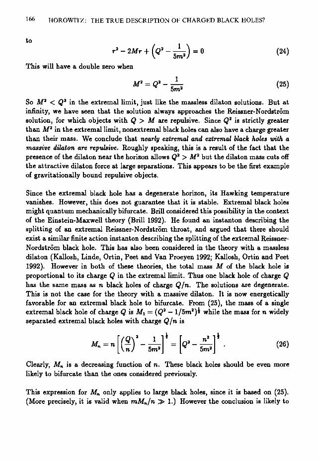
166 HOROWITZ: THE TRUE DESCRIPTION OF CHARGED BLACK HOLES?
to
( 5 ? ) - o <24>This will have a double zero when
^ <25>
So M2 < Q2 in the extremal limit, just like the massless dilaton solutions. But atinfinity, we have seen that the solution always approaches the Reissner-Nordstromsolution, for which objects with Q > M are repulsive. Since Q2 is strictly greaterthan M2 in the extremal limit, nonextremal black holes can also have a charge greaterthan their mass. We conclude that nearly extremal and extremal black holes with amassive dilaton are repulsive. Roughly speaking, this is a result of the fact that thepresence of the dilaton near the horizon allows Q2 > M2 but the dilaton mass cuts offthe attractive dilaton force at large separations. This appears to be the first exampleof gravitationally bound repulsive objects.
Since the extremal black hole has a degenerate horizon, its Hawking temperaturevanishes. However, this does not guarantee that it is stable. Extremal black holesmight quantum mechanically bifurcate. Brill considered this possibility in the contextof the Einstein-Maxwell theory (Brill 1992). He found an instanton describing thesplitting of an extremal Reissner-Nordstrom throat, and argued that there shouldexist a similar finite action instanton describing the splitting of the extremal Reissner-Nordstrom black hole. This has also been considered in the theory with a masslessdilaton (Kallosh, Linde, Ortin, Peet and Van Proeyen 1992; Kallosh, Ortin and Peet1992). However in both of these theories, the total mass M of the black hole isproportional to its charge Q in the extremal limit. Thus one black hole of charge Qhas the same mass as n black holes of charge Q/n. The solutions are degenerate.This is not the case for the theory with a massive dilaton. It is now energeticallyfavorable for an extremal black hole to bifurcate. From (25), the mass of a singleextremal black hole of charge Q is Mi = (Q2 — l/5ra2)^ while the mass for n widelyseparated extremal black holes with charge Q/n is
Clearly, Mn is a decreasing function of n. These black holes should be even morelikely to bifurcate than the ones considered previously.
This expression for Mn only applies to large black holes, since it is based on (25).(More precisely, it is valid when mMn/n S> 1.) However the conclusion is likely to

HOROWITZ: THE TRUE DESCRIPTION OF CHARGED BLACK HOLES? 167
hold more generally. This is because it follows from the fact that extremal blackholes are repulsive, which in turn is a consequence of two general properties of theextremal solutions: they always approach Reissner-Nordstrom asymptotically andhave Q2 > M2. Thus extremal black holes will probably continue to bifurcate untilthey have a single unit of charge. At this point the black hole is small comparedto the Compton wavelength of the dilaton, Mm <C 1. (Black holes of this typecan also be obtained by starting with a large hole with small charge, and letting itevaporate. The extremal limit will not be reached until Mm < 1 . ) For these smallblack holes there is a region M <C r <C l/m which is far from the black hole butinside the dilaton Compton wavelength. One can solve the dilaton equation (26)exactly for r 3> M since the spacetime is essentially flat. The result is that forM <C r <C 1/fn, $ behaves like a massless dilaton: <f> oc 1/r. So one expects theblack holes to behave qualitatively like the massless dilaton solution discussed in theprevious section. Numerical calculations confirm that this is indeed the case (Homeand Horowitz 1992). In particular, there is no inner horizon and in the extremallimit, the event horizon shrinks to zero area and becomes singular. The string metricdescribing an extremal magnetically charged black hole has an infinite throat.
We have seen that black holes with a massive dilaton can be viewed as interpolatingbetween the Reissner-Nordstrom solution (when their mass is large), and the masslessdilaton solution (when their mass is small). One can say something about the tran-sition region Mm « 1 by considering when a degenerate horizon can exist. If thereis a radius r0 for which A and A' both vanish, the field equations yield the followingcondition on the value of <f> at r0
e2* ^ ,- O2m2 (Tl\
The left hand side has a minimum of e2/4 when ^ = 1. So for Q2m2 < e2/4, therecannot exist a degenerate horizon. For Q2m2 > e2/4 there are two possible values of</>} but the equations of motion also imply that A" oc (1 — ^) so one needs <f> < 1 tohave A" > 0 as required for an event horizon. At the critical value, Q2m2 = e2/4,A" also vanishes yielding a triple horizon. This suggests that there may be solutionswith three distinct horizons. But at the moment, there is no direct evidence for this.
These intermediate size black holes can have an unusual property when described interms of the string metric. One can show that the radius of the spheres of sphericalsymmetry in the Einstein metric, J?, is monotonically increasing outside the horizonas expected. In the string metric, the radius of the spheres is Re*. For an electricallycharged hole, it turns out that </> is also increasing outside the horizon so the spheresindeed become larger as r increases. However, for a magnetically charged hole, <f>changes sign and is monotonically decreasing outside the horizon. So Re* need not

168 HOROWITZ: THE TRUE DESCRIPTION OF CHARGED BLACK HOLES?
be an increasing function of r. It certainly increases near infinity, and for the masslessdilaton solution (18), it is monotonically increasing everywhere. However, for nonzerodilaton mass, one can show that it decreases outside the horizon for nearly extremalblack holes with Mm « 1. This means that the spatial geometry contains a wormhole.Unlike the familiar wormhole in the maximally extended Schwarzschild solution, thiswormhole is outside the horizon. It is static and transversable.
Combining this with our previous results, we see that the string metric describing anextremal, magnetically charged black hole has a rather exotic dependence on mass. Itresembles the Reissner-Nordstrom metric with a degenerate horizon when Mm » 1.A wormhole forms outside the degenerate horizon when Mm » 1. Finally, the horizonand wormhole both disappear and are replaced by an infinite throat when Mm «C 1.
4 CONCLUSIONSWe have discussed two related issues. On the mathematical side, we have seen thatdespite the apparent complication introduced by a massless dilaton, the theory sharessome of the features of the Einstein-Maxwell theory. In particular, there is a solutiongenerating transformation which is remarkably similar to the Harrison transforma-tion. The resulting extremal black hole can be viewed as the "square root" of theextremal Reissner-Nordstrom solution. On the physical side, we have seen that theevolution of charged black holes predicted by string theory is quite different fromstandard lore. Black holes initially (when Mm > 1) are quite similar to the Reissner-Nordstrom solution. But as they evolve (through Hawking evaporation and possiblequantum bifurcation) they reach a stage where Mm <C 1. At this point, the blackholes are similar to the massless dilaton solutions. For a dilaton mass of m = ITeV,the transition will occur at a black hole mass of M = 10ngms which is well above thePlanck scale. This ensures that Planck scale corrections, which have been neglectedthroughout, will still be negligible.
What is the most likely endpoint of this evolution? Assuming the charge is notcompletely radiated away, one expects to be left with an extremal black hole withunit charge. (Although likely, this is still uncertain due to the fact that the Hawkingtemperature does not vanish as one approaches the extremal limit of these small blackholes.) Since charge is quantized, this must be stable against further bifurcation.These remnants would be pointlike objects, with charge greater than their mass,which repel each other. In other words, they would appear very much like elementaryparticles. (See also Holzhey and Wilczek 1992.) In fact, by shifting the dilatonpotential so that its minimum is at <f>0 ^ 0, one can change the charge to mass ratioof the extremal black holes. There even exists a value of <f>0 such that the extremalblack hole of unit charge has the mass of an electron. In the past, one of the main

HOROWITZ: THE TRUE DESCRIPTION OF CHARGED BLACK HOLES? 169
objections to interpreting an electron as a black hole was the fact that its charge ismuch larger than its mass (in geometrical units) so that according to the Reissner-Nordstrom solution, it would be a naked singularity. The massive dilaton predictedby string theory removes this objection and opens up the possibility of a much closerconnection between elementary particles and black holes.
ACKNOWLEDGMENTSIt is a pleasure to thank my collaborators D. Garfinkle, A. Strominger, and especiallyJ. Home. This work was supported in part by NSF Grant PHY-9008502.
REFERENCES
Banks T, Dabholkar A, Douglas M and O'Loughlin M (1992) "Are Horned Particlesthe Climax of Hawking Evaporation?", Phys. Rev. D45 3607
Banks T and O'Loughin M (1992) "Classical and Quantum Production of Cornuco-pions at Energies Below 1018 GeV", Rutgers preprint RU-92-14, hep-th/9206055
Banks T, O'Loughin M, and Strominger A (1992) "Black Hole Remnants and theInformation Puzzle", Rutgers preprint RU-92-40, hep-th/9211030
Bekenstein J (1972) "Nonexistence of Baryon Number for Static Black Holes", Phys.Rev. D5 1239
Brill D (1992) "Splitting of an Extremal Reissner-Nordstrom Throat via QuantumTunneling", Phys. Rev. D46 1560
Brill D and Horowitz G (1991) "Negative Energy in String Theory", Phys. Lett.B262 437
Brill D and Pfister H (1989) "States of Negative Total Energy in Kaluza-Klein The-ory", Phys. Lett. B228 359
Chase J (1970) "Event Horizons in Static Scalar-Vacuum Spacetimes", Commun.Math. Phys. 19 276
Garfinkle D (1992), private communication.
Garfinkle D, Horowitz G and Strominger A (1991) "Charged Black Holes in StringTheory," Phys. Rev. D43 3140; (1992) D45, 3888(E)

170 HOROWITZ: THE TRUE DESCRIPTION OF CHARGED BLACK HOLES?
Gibbons G (1982) "Antigravitating Black Hole Solitons with Scalar Hair in N=4Supergravity", Nucl. Phys. B207 337
Gibbons G and Maeda K (1988) "Black Holes and Membranes in Higher-DimensionalTheories with Dilaton Fields", Nucl. Phys. B298 741
Gregory R and Harvey J (1992) "Black Holes with a Massive Dilaton", Enrico FermiPreprint EFI-92-49, hep-th /9209070
Harrison B (1968) "New Solutions of the Einstein-Maxwell Equations from Old", J.Math. Phys. 9 1744
Hartle J and Hawking S (1972) "Solutions of the Einstein-Maxwell Equations withMany Black Holes", Commun. Math. Phys. 26 87
Harvey J and Strominger A (1992) "Quantum Aspects of Black Holes", to appear inthe proceedings of the 1992 Trieste Spring School on String Theory and QuantumGravity, hep-th/9209055
Hassan S and Sen A (1992) "Twisting Classical Solutions in Heterotic String Theory",Nucl. Phys. B375 103
Holzhey C and Wilczek F (1992) "Black Holes as Elementary Particles", Nucl. Phys.B380 447
Home J and Horowitz G (1992) "Black Holes Coupled to a Massive Dilaton", Nucl.Phys. B to appear, hep-th/9210012
Horowitz G (1992) "The Dark Side of String Theory: Black Holes and Black Strings",to appear in the proceedings of the 1992 Trieste Spring School on String Theoryand Quantum Gravity, hep-th/9210119
Israel W (1968) "Event Horizons in Static Electrovac Spacetimes", Commun. Math.Phys. 8 245
Kallosh R, Linde A, Ortin T, Peet A and Van Proeyen A (1992) "Supersymmetry asa Cosmic Censor", Stanford preprint SU-ITP-92-13
Kallosh R, Ortin T and Peet A (1992) "Entropy and Action of Dilaton Black Holes",Stanford preprint SU-ITP-92-29, hep-th/9211015

HOROWITZ: THE TRUE DESCRIPTION OF CHARGED BLACK HOLES? 171
Maharana J and Schwarz J (1992) "Noncompact Symmetries in String Theory",Caltech preprint CALT-68-1790, hep-th/9207016
Majumdar S (1947) Phys. Rev. 72 930
Papapetrou A (1947) Proc. Roy. Irish Acad. A51 191
Sen A (1992) " Black Holes and Solitons in String Theory", Tata preprint TIFR-TH-92-57, hep-th/9210050

Limits on the Adiabatic Index in Static Stellar Models
LEE LINDBLOM AND A.K.M. MASOOD-UL-ALAM
Physics Department, Montana State University, Bozeman, Montana 59717
1 SUMMARYDieter Brill has made important contributions to the study of the positive masstheorem in general relativity theory (Brill 1959) and to the analysis of the conformalproperties of asymptotically flat space-times (Cantor &; Brill 1981). It is a pleasureto honor him on this occasion by applying these analytical tools to the study of staticstellar models. We use the positive mass theorem and the conformal properties ofthese spacetimes to deduce an interesting constraint on the allowed values of theadiabatic index in the static stellar models of general relativity theory.
It is well known that non-singular polytropic stellar models in the Newtonian theorycan exist only if the adiabatic index of the fluid is sufficiently large, 7 > 6/5 (or equiv-alently if the polytropic index is sufficiently small, n < 5; see e.g., Chandrasekhar1939). In this paper we derive two limits on the allowed values of the adiabatic indexin the stellar models of general relativity theory. Our limits apply to static stellarmodels that have a finite radius and an equation of state which satisfies certain fairlyweak smoothness assumptions. Our first bound on the adiabatic index guaranteesthat
at some points in every neighborhood of the surface of such stars. This limit, althoughweaker than the traditional Newtonian limit, is simply a consequence of the regularityof the spacetime at the surface of these stars. This result makes no assumption aboutthe high-density portion of the equation of state. Thus it applies to (essentially) everystatic stellar model in general relativity theory. Our second bound on the adiabaticindex guarantees that
§ 2 \ (2,
172

LINDBLOM AND MASOOD-UL-ALAM: LIMITS ON THE ADIABATIC INDEX 173
in some portion of every static stellar model with finite radius. This result is the directgeneral-relativistic analogue of the Newtonian limit 7 > 6/5 for spherical polytropicstars with finite radius. Our result is considerably more general, however, because wedo not assume that the equation of state is polytropic (i.e., of the form p = Kp1+1/n
where K and n are constants). Our result is also more general because it does notassume that the stellar model has spherical symmetry. Thus, our result complimentsthe work on the necessity of spherical symmetry in static general-relativistic stellarmodels by Masood-ul-Alam (1988) and by Beig & Simon (1991, 1992). Those proofsof spherical symmetry specifically exclude any equation of state which violates equa-tion (2) at any point within the star. Thus, our second bound eliminates a large classof potential counterexamples to the spherical-symmetry conjecture. In particular,our result shows that no stellar model whose equation of state violates equation (2)everywhere can exist in general relativity theory.
2 THE SURFACE LIMITA stellar model in general relativity theory is an asymptotically-flat spacetime thatsatisfies Einstein's equation with a perfect-fluid source. A static (i.e., time inde-pendent and non-rotating) stellar model has a time-translation symmetry (by as-sumption) whose trajectories are hypersurface orthogonal. Thus, coordinates may bechosen in which the spacetime metric tensor has the representation
ds2 = -V2dt2 + gabdxadx\ (3)
where V and the three-dimensional spatial metric gab are independent oft. The topol-ogy of the constant-f hypersurfaces must be R3 (Lindblom & Brill 1980, Masood-ul-Alam 1987a). Einstein's equation for static stellar models reduces in this representa-tion to the pair of equations
3p), (4)Rab = V~lDaDhV + 4TT(P - p)gab. (5)
The density and pressure of the fluid are denoted p and p\ and the density is assumedto be a given function of the pressure, p = p(p) (the equation of state), which isnon-negative and non-decreasing. The spatial covariant derivative compatible withgab is denoted Da, and its Ricci curvature is denoted Rah. The Bianchi identity forthe three-dimensional spatial geometry may be reduced to the form
, (6)
with the use of equations (4)-(5).

174 LINDBLOM AND MASOOD-UL-ALAM: LIMITS ON THE ADIABATIC INDEX
The surface of a stellar model is the boundary between the interior fluid region wherethe pressure is positive, and the exterior region where the vacuum Einstein equationis satisfied. We limit our consideration here to stars whose surfaces occur at a finiteradius (i.e., to stars which have non-trivial exterior vacuum regions). The pressuremust vanish on the surface of the star in order to insure that the spacetime is non-singular there. We first prove that the ratio p/p must also vanish on this surface:Consider a smooth curve xa(X) that lies inside the star for Ao < A < A5, while thepoint xa(Xs) lies on the surface. Let na = dxa/d\ denote the tangent to this curve.We evaluate the integral of (p + p)~lnaDap along this curve using equation (6):
/•**> dp [> n°Dapd\ f* naDaVd\ \V(\o)] ( )
JpiXo)p(P)+P Ao p + p Jx0 V °S[v(A)J" U
In the limit A —• A the expression on the right is well behaved, thus, the integral onthe left must also be well behaved. Consequently the function,
h{p) = IJo
* (8)o p(p)+pJ
is well defined for all p within any static stellar model in general relativity theory.The equation of state, p(p), is a non-decreasing function; thus, we may estimate h(p)as follows,
Jo p(p)+p Jo p(p)+p
Since limp_+0+ h(j>) = 0, we conclude from equation (9) that
0 = lim eh(p) - 1 > lim - . (10)P-+0+ p-+0+ p
Thus, the limit of p/p must vanish. So, we have established the desired result:
Lemma. Consider a static stellar model in general relativity theory whose surfaceoccurs at a finite radius. Assume that the equation of state p = p(p) is a positiveand non-decreasing function in some open neighborhood of the surface of the star:i.e., for pressures 0 < p < e. Then limp_+0+ (p/p) = 0.
We now turn to the derivation of our first limit on the adiabatic index,

LINDBLOM AND MASOOD-UL-ALAM: LIMITS ON THE ADIABATIC INDEX 175
We assume that the equation of state, p(p), is a positive and non-decreasing C1
function in the open interval, 0 < p < e (for some e > 0). Thus, l/7(p) is acontinuous and non-negative function there. Let T(e) be the least upper bound ofj(p) for 0 < p < e: i.e., let F(e) = sup 0<p<c7(p)- If T(6) *s n o t finite, then there existpoints in the open interval 0 < p < e where 7 > 1, trivially. We turn our attention,therefore, to the case where T(e) is finite. From the definition of the adiabatic index,we obtain the following inequality
This inequality may be integrated to obtain an upper bound for the density functionon the open interval 0 < p < e:
P < p(e)(f)1/r(e)• (13)
This upper bound and the Lemma may then be used to obtain the following conditionon r(e),
' " " ' 1 / r W . (14)i m > i i m-+0+ p "" p->o+ p(e)
The limit on the right vanishes only if F(e) > 1. Since limp^0+(p/p) = 0 as aconsequence of the Lemma, it follows that F(e) > 1. Thus there exist points in theopen interval 0 < p < e where 7 > 1. The constant e may be chosen to be arbitrarilysmall, so there must exist points in every open neighborhood of the surface of thestar where 7 > 1. In summary then our first limit on the adiabatic index is:
Theorem 1. Consider a static stellar model in general relativity theory whose surfaceoccurs at a finite radius. Assume that the equation of state p = p(p) is a positiveand non-decreasing C1 function of the pressure in some neighborhood of the surfaceof the star, 0 < p < e. Then the adiabatic index j(p) > 1 at some point in everyopen neighborhood of the surface of the star.
3 THE MAXIMUM LIMITOur method for deriving a limit on the maximum value of the adiabatic index isvery similar to the technique developed by Masood-ul-Alam (1987b) for proving thenecessity of spherical symmetry in certain static stellar models. We construct aparticular conformal factor which is used to transform the spatial metric gab. Thisconformal factor scales the mass associated with the spatial geometry to zero whileleaving the transformed scalar curvature non-negative—unless the adiabatic index of

176 LINDBLOM AND MASOOD-UL-ALAM: LIMITS ON THE ADIABATIC INDEX
the fluid is sufficiently large. For stellar models composed of fluid with small adiabaticindex, then, the positive mass theorem implies that the transformed geometry is flat.We show, however, that this is inconsistent with our assumption that the stellar modelhas a finite radius. Thus, we conclude that the maximum value of the adiabatic indexmust exceed a certain lower bound in every static stellar model with a finite radius.
The Bianchi identity, equation (6), for static fluid spacetimes determines a functionalrelationship between the fluid variables, p and p, and the potential V. In particular,with the aid of equations (7)-(8), the density and pressure may be expressed asexplicit functions of V: p(V) = / r ^ l o g ^ / V ) ] , and p(V) = p\p(V)], where Vs is thevalue of the potential on the surface of the star. We use these functions to define aconformal factor rp in the interior region of the star (where 0 < V < Vs):
If the interior of the star is composed of more than one connected region, then ip(V)is defined in each region by equation (15) with the constant Vs taken to be the surfacevalue of V for that region. In the exterior of the star (e.g., where Vs < V < 1) wedefine the conformal factor to be,
^(V) = \(l + V). (16)
It is easy to see that this conformal factor is continuous across each component ofthe surface of the star by setting V = Vs in equations (15) and (16). It is alsostraightforward to verify that dip/dV is continuous at the surface of the star. Thederivative of \p in the interior of the star satisfies the equation
dV
Using the result of the Lemma, lim V-*vs(p/p) = 0, it is easy to take the limit of theright side of equation (17) to verify that dtp/dV = 1/2 at the surface of the star. Thesecond derivative d2ip/dV2 vanishes in the exterior of the star, while it is given bythe expression
Vstl>V2{1 + VS){1 + Zp/p)2
in the interior of the star. The function d2tp/dV2 is continuous and has a finite upperbound for V <VS whenever I/7 is bounded. Thus, xp is C u (i.e, its first derivative

LINDBLOM AND MASOOD-UL-ALAM: LIMITS ON THE ADIABATIC INDEX 177
satisfies a Lipshitz condition) even across the surface of the star as long as I/7 isbounded. Note that l//y(p) is finite for any p > 0 as a consequence of our assumptionthat p{p) is a C1 function. Thus, our assumption that I/7 is bounded is a restrictionon the behavior of the equation of state only near p = 0. The boundedness of I/7follows automatically for equations of state which are smooth enough that the limitof 7(p) is well defined (in the sense that lim inf 7 = lim sup 7) as p —> 0+. In thiscase Theorem 1 implies that lim inf 7 > 1, and so I/7 is bounded as p —• 0"1".
We use the function ip given in equations (15) and (16) to define a conformallytransformed spatial metric tensor gab:
gab = ip4gab- (19)
This transformed metric has two important properties: a) the mass associated withgab is zero; and b) the scalar curvature associated with gab is non-negative unless theadiabatic index is too large. The first of these properties can be deduced by examiningthe asymptotic boundary conditions on the stellar model. In general relativity theorya stellar model is a non-singular asymptotically-flat solution to equations (4)-(5). Theappropriate asymptotic forms for V and gab are therefore,
V = l - — + O(r~ 2), (20)r
) b + O(r-2), (21)
where the constant M is the mass of the star, 6ab is the flat Euclidean metric, andr is a spherical radial coordinate associated with the metric 6ab. These asymptoticforms imply that the conformal factor defined in equation (16) has the asymptoticform
* = 1 - fr + °(*-2)- (22)It follows, then, that the asymptotic form of the transformed metric is
9ab = Sab + 0{r~2). (23)
Thus, the mass associated with gab is zero. The second important property of gab, thesign of its scalar curvature, is easily deduced. The general expression for the scalarcurvature R associated with the metric gab is
R = 8^"5 (27rpV - DaDail)). (24)

178 LINDBLOM AND MASOOD-UL-ALAM: LIMITS ON THE ADIABATIC INDEX
The term DaDaip can be evaluated by using equations (4) and (15)-(18). The resultcan be expressed in the form
in the interior of each connected component of the star, while R vanishes in theexterior of the star. The potential on the surface of the star is strictly less thanone, Vs < 1, in any stellar model that has a finite radius. Thus, the conformallytransformed scalar curvature is non-negative as long as the condition,
is satisfied by the adiabatic index.
The positive mass theorem (Schoen &; Yau 1979, Parker & Taubes 1982) impliesthat a C1'1 asymptotically-flat Riemannian three-metric is flat if its scalar curvatureis non-negative and its mass is zero. The needed smoothness of gab follows fromthe smoothness of ip established above. Thus, the spatial metric gab is flat if theadiabatic index satisfies equation (26). But, if gab is flat, then the scalar curvature Rvanishes. This implies, from equation (25), that V = 1 and that equality must holdin equation (26). But Vs < 1 in any star with a finite radius, and so we conclude thatR must be negative somewhere in such stars. Thus equation (26) must be violated.Consequently, at some point in every static star with a finite radius the adiabaticindex must satisfy
In summary, then, we have established the following lower bound on the maximumvalue of the adiabatic index:
Theorem 2. Consider a static stellar model in general relativity theory whose surfaceoccurs at a finite radius. Assume that the equation of state p = p(p) is a positiveand non-decreasing C1 function of the pressure. Assume that l/7(p) is bounded asp —• 0+. Then the adiabatic index must satisfy the inequality
at some point within the star.

LINDBLOM AND MASOOD-UL-ALAM: LIMITS ON THE ADIABATIC INDEX 179
We point out that the extreme case in the argument that leads to Theorem 2—whenequality holds in equation (26) and Vs = 1—is not vacuous. This case constrainsthe equation of state of the fluid to be the one used by Buchdahl (1964) to constructa family of non-singular but infinite-radius stellar models. The existence of theseasymptotically flat, albeit infinite radius, stellar models suggests that our limit onthe maximum value of the adiabatic index is the strongest possible limit of this kind.
4 CONCLUDING REMARKSIt is instructive to examine the implications of Theorem 2 for stellar models con-structed from fluid that has a polytropic equation of state:
p = KP1+1/n, (29)
where K and n are constants. The constraint on the adiabatic index, equation (28),is equivalent for poly tropes to a constraint on the polytropic index n:
n < 5 ( l + 6p//?)"1 < 5 . (30)
Thus, n < 5 for general-relativistic stellar models that have a polytropic equationof state. This shows that equation (28) is the direct general-relativistic analogueof the familiar Newtonian limit on the polytropic index n < 5 (see e.g., Chan-drasekhar 1939).
We have chosen to express the limit on the adiabatic index, equation (28), in a formwhich involves only the equation of state without making any reference to the macro-scopic properties of the particular stellar model. In fact, a somewhat stronger limitwas obtained in equation (27). That limit on the adiabatic index can be expressedin another form that involves the surface value of the potential Vs in a simple way:
7>3^>| (31)2 + 6V 0
Thus, for a spherical star of mass M and radius R the adiabatic index must satisfythe inequality
6
5 ' { j
at some point within the star. For polytropic stars this condition is equivalent to thebound

180 LINDBLOM AND MASOOD-UL-ALAM: LIMITS ON THE ADIABATIC INDEX
n < 2 + 3VS = 2 + 3(1 - 2M/R)1/2 < 5, (33)
on the polytropic index.
The limits on the adiabatic index that we derive in this paper are necessary conditionsfor the existence of a static stellar model in general relativity theory. Our limits areweaker, therefore, than the bounds needed to guarantee the stability of these models.Glass and Harpaz (1983) have shown, for example, that the adiabatic index mustexceed 4/3 in a stable relativistic polytrope by an amount that depends on the ratiop/p at the center of the star. A similar limit on a suitably averaged value of theadiabatic index, 7 > 4/3, is necessary for the stability of nearly Newtonian stars withany equation of state (see e.g., Misner, Thorne & Wheeler 1973).
The bound on the adiabatic index derived in Theorem 2 does not assume that thestellar model has spherical symmetry. Thus, our result compliments the work onthe necessity of spherical symmetry in static general-relativistic stellar models byMasood-ul-Alam (1988) and by Beig & Simon (1991, 1992). Those proofs of spheri-cal symmetry apply only to equations of state for which the adiabatic index satisfiesthe inequality (28) at every point. Thus, Theorem 2 eliminates a large class of poten-tial counterexamples to the spherical-symmetry conjecture. In particular, our resultshows that no stellar model whose equation of state violates equation (28) every-where can exist in general relativity theory. Of course many equations of state exist,including many realistic models of neutron-star matter, which satisfy equation (28)for some values of the pressure and violate it for others.
This research was supported by the grant PHY-9019753 from the National ScienceFoundation, and grant NAGW-2951 from the National Aeronautics and Space Ad-ministration.
REFERENCESBeig, R. k Simon, W. 1991, Lett. Math. Phys., 21, 245-250.Beig, R. Sz Simon, W. 1992, Commun. Math. Phys. 144, 373-390.Brill, D.R. 1959, Ann. Phys. 7, 466-483.Buchdahl, H.A. 1964, Ap. J. 140, 1512-1516.Cantor, M., k Brill, D.R. 1981, Comp. Math. 43, 317-330.Chandrasekhar, S. 1939, An Introduction to the Study of Stellar Structure, (Chicago:
University of Chicago Press).Lindblom, L. & Brill, D.R. 1980, in Essays in General Relativity, pp. 13-19, ed. by
F.J. Tipler, (New York: Academic Press).

LINDBLOM AND MASOOD-UL-ALAM: LIMITS ON THE ADIABATIC INDEX 181
Masood-ul-Alam, A.K.M. 1987a, Commun. Math. Phys. 108, 193-211.Masood-ul-Alam, A.K.M. 1987b, Class. Quantum Grav. 4, 625-633.Masood-ul-Alam, A.K.M. 1988, Class. Quantum Grav. 5, 409-421.Misner, C.W., Thorne, K.S. & Wheeler, J.A. 1973, Gravitation, (San Francisco: W.H.
Freeman and Co.).Parker, T. & Taubes, C. 1982, Commun. Math. Phys. 84, 223-238.Schoen, R. & Yau, S.T. 1979, Commun. Math. Phys. 65, 45-76.

On the Relativity of Rotation
BAHRAM MASHHOON
Department of Physics and AstronomyUniversity of Missouri-ColumbiaColumbia, Missouri 65211, USA
ABSTRACT
The problem of the origin of rotational inertia is examined within the framework ofthe relativistic theory of gravitation. It is argued that gravitomagnetic effects cannotbe interpreted in terms of the relativity of rotation. Absolute and relative motionare discussed on the basis of the hypothesis that these are complementary classicalmanifestations of movement.
What is the origin of inertia? For instance, with respect to what does the Earthrotate around its axis? The rotation of a body does not generate any basic new grav-itational effect in the Newtonian theory. This is not the case, however, in Einstein'stheory of gravitation. The striking analogy between Newton's law of gravitation andCoulomb's law of electricity has led to a description of Newtonian gravity in termsof a gravitoelectric field. Any theory that combines Newtonian gravity with Lorentzinvariance is expected to contain a gravitomagnetic field in some form; in generalrelativity, the gravitomagnetic field is usually caused by the angular momentum ofthe source of the gravitational field. The first gravitomagnetic effects were describedby de Sitter1 soon after Einstein's fundamental work on general relativity. The ques-tion of relativity of rotation was also discussed by de Sitter following his investigationof the astronomical consequences of Einstein's relativistic theory of gravitation; deSitter concluded that the problem of inertia did not have a solution in the generaltheory of relativity.1 There is no direct experimental evidence for the existence of thegravitomagnetic field at present; however, various proposals exist for measuring thegravitomagnetic field of the Earth. The most significant proposal has developed intothe Gravity Probe B which will involve a telescope and a superconducting gyroscopeon board a drag-free satellite in a polar orbit about the Earth.2'3
In connection with the origin of rotational inertia, an attempt is made here to describethe physical origin of the gravitomagnetic field in terms of relativity of rotation within
182

MASHOON: ON THE RELATIVITY OF ROTATION 183
the framework of the standard relativistic theory of gravitation that is consistent withall of the observational data available at present, namely, Einstein's general theory ofrelativity. The problem may be described as follows: Imagine an idealized situationinvolving an isolated astronomical body (henceforth called "Earth") whose center-of-mass is at rest in an appropriate system of coordinates. If the Earth is static, thereis only a gravitoelectric field which consists of the Newtonian part together with thepost-Newtonian relativistic corrections. Now suppose that the Earth rotates rigidlywith constant frequency ue around its axis, then a gravitomagnetic field exists inaddition to the gravitoelectric field. However, a coordinate system may be chosenin which the rotating Earth is completely at rest; this comoving system is in factthe fundamental astronomical coordinate system that has been employed since timeimmemorial. In this system the Earth appears to be the center of the universe sincethe heavens revolve around it. According to general relativity, the gravitomagneticfield of the Earth is still present in this coordinate system; in fact, an experiment hasbeen proposed to measure this field by a Foucault pendulum located at the southpole.4 With respect to comoving observers at rest on the Earth, the gravitomagneticfield should be interpreted as the induced field of the moving heavens if rotationis relative. Is such an interpretation permitted by the general theory of relativity?If not, then the rotation of the Earth must be considered to be absolute accordingto general relativity. The gravitomagnetic field would thus be a manifestation ofthe absolute rotation of the Earth. It is argued in this work that the rotation ofthe Earth is absolute; in general, the translational and rotational accelerations of aphysical system are absolute.5 Mach's fundamental insight6 is interpreted instead inlight of the quantum theory.7 Neither relative motion nor absolute motion can providea completely satisfactory description of physical phenomena. Movement of a physicalsystem has complementary classical manifestations in relative and absolute motion.
It is a great pleasure for me to dedicate this paper to Dieter R. Brill on the occasionof his sixtieth birthday.
1. INTRODUCTIONThe description of observers and their motion in spacetime is of basic importance fora proper discussion of the notion of relativity of arbitrary motion. The path of anobserver, i.e., a classical measuring device, in space and time is characterized by itsworldline x** — x^(r), where r is the proper time along the path. The idealizationof replacing an extended classical system by a geometrical line is necessary for theo-retical purposes; however, this does not appear to constitute a fundamental physicallimitation.8'9 To perform physical measurements over an extended period of time,an observer must define a local spatial coordinate system at each instant of time;this requirement implies that a tetrad frame A^ must be carried along the path of

184 MASHOON: ON THE RELATIVITY OF ROTATION
the observer such that A ^ is a unit vector tangent to the path and constitutes thelocal temporal axis and \fo are unit vectors that constitute the local spatial axes.10
The motion of the orthonormal frame A ^ along the path may be described by anantisymmetric Lorentz tensor <f>ap,
which describes the deviation of the frame from parallel transport along the path.The tensor <f)a(3 can be decomposed in a natural way in terms of two local Cartesianvectors g and u , (f)a(3 —> (g , « ) , which represent, respectively, the local translationalacceleration of the observer and the rotational frequency of the spatial frame withrespect to a nonrotating (i.e., Fermi-Walker transported) triad. This interpretationof the "electric" and "magnetic" parts of the antisymmetric tensor <j>ap is based onthe following considerations. Let A ^ = dx^ jdr be the velocity vector, then
Adr' +T>">dT dr
where A** is the acceleration vector of the observer, and A^ = A^Xfa = (0, —g)since A^ is a unit timelike vector and hence A*1, A^A^ = 0, is spacelike. Thus<f>oi = —gi and g2 = A^A** is the square of the magnitude of the acceleration vector.The signature of the spacetime metric is +2 throughout. While the "electric" partof (f)af3 determines the translational acceleration of the observer, the "magnetic" partdetermines its rotational frequency. Imagine that the observer carries along its patha triad of ideal gyroscopes that establish a local nonrotating spatial frame. Let thisorthonormal tetrad system be denoted by A£ , where A ox = A^ and DXfa/Dr ispurely tangential, i.e.
DX**—— = A^AyA^ — A^TJoa . (3)
Any other orthonormal tetrad frame is related to the nonrotating system by a simplerotation of the spatial triad, i.e., A^ = iJ^-A^, where
^ = <M4; , (4)
so that the "magnetic" part of (j)ap determines the rate of rotation of the actualframe with respect to the nonrotating system. The frequency of rotation is given by
It is important to recognize that g and a; are scalars, i.e., they are totally independentof the underlying coordinate system employed in spacetime. The observer may per-ceive itself to be at rest and interpret its measurements in terms of the "acceleration"

MASHOON: ON THE RELATIVITY OF ROTATION 185
and "rotation" of the rest of the masses in the universe toward it; however, this inter-pretation will not change the fact that the observer has at each instant an absolutetranslational acceleration g(r) and an absolute rotation of frequency O;(T). The abso-lute character of translational and rotational accelerations may be expressed in termsof the existence of absolute acceleration lengths that may be associated with the ob-server. In fact, all actual observers are endowed with acceleration lengths; however,it is important to imagine locally inertial observers that have infinite accelerationlengths. Such ideal observers follow geodesies and refer their measurements to locallynonrotating spatial frames. For an accelerated observer referring its measurements toa nonrotating frame, the proper (translational) acceleration length is c2/g(r) whilefor a geodesic observer that refers its measurements to a rotating frame the proper(rotational) acceleration length is C/LO(T). In general, the proper acceleration scalesmay be defined11 in terms of the Lorentz invariants of </>a/3, i.e., <f>ap<t>al3 = 2(—# 2 +UJ2)and <t>*ap<t>aP = 4g a;, where (f)*a(3 is the dual of </>ap.
The theoretical origin of these absolute (translational and rotational) accelerationscan be traced back to the fact that in Newtonian mechanics an observer can decideby purely local measurements whether it is noninertial. That is, the local laws ofmotion already embody the fundamental Newtonian notions of absolute space andtime. Therefore, it should not be surprising that the relativistic generalization ofthe Newtonian equation of motion still contains the notion of absolute acceleratedmotion. It should be clear from this analysis that general relativity simply inheritsthe essential aspects of Newtonian theory's problem of the origin of inertia.5
The determination of spacetime metric is the basic theoretical requirement underlyingthe construction of an orthonormal tetrad associated with an ideal test observer. Themetric tensor g^v satisfies the gravitational field equations
which are nonlinear partial differential equations for the metric tensor once theenergy-momentum tensor of matter, T^, is specified. To obtain a definite solution,boundary conditions are needed. It appears natural to impose boundary conditionson g^y at infinity. However, it is likely that the actual physical conditions at infinitywill never be known.1 Therefore, the imposition of boundary conditions amounts torestrictions on the solutions of the field equations in order to choose from all possiblesolutions only those that have actual physical relevance. The main experimental suc-cesses of general relativity are related to those solutions of the field equations thatare asymptotically flat. This naturally corresponds to the notion that spacetime isMinkowskian; however, where mass-energy exists, the spacetime curvature deviatesfrom zero in a certain proportion to the accumulation of mass-energy. In this ap-

186 MASHOON: ON THE RELATIVITY OF ROTATION
proach, the absolute space and time of Newton are thus replaced by Minkowski'sabsolute spacetime; however, no at tempt is made to account for this underlying con-t inuum.
To avoid the introduction of a global Minkowski spacetime, the hypothesis has beenintroduced tha t the universe is spatially closed.12'13 Spatial closure depends upon theexistence of sufficient mass-energy in the world. Observations do not compel us tochoose a spatially closed cosmos at the present time; however, the adoption of spatialclosure has led to elegant analyses of the dynamics of the gravitational field.14'15
It can be shown that the idea of relativity of arbitrary motion is at variance withgeneral relativity regardless of the boundary conditions. In fact, it may eventuallyturn out tha t even a spatially closed world is also compatible with the existence ofan underlying Minkowski spacetime (cf. section 4).
The basic physical steps leading from the Newtonian theory to the relativistic the-ory of gravitation have been delineated in a recent work16 on the basis of the theoryof measurement. The analysis of measurements provides a firm foundation for thediscussion of the relativity of arbitrary motion in the theory of general relativity.The structure of spacetime is determined by the energy-momentum tensor of mat-ter as well as the boundary data in general relativity; therefore, it might appearnatural to suppose that the absolute translational and rotational accelerations of anobserver occur relative to the mass-energy content of the universe.12'17 The relativ-ity of translational acceleration has been examined in a recent work5 and found tobe incompatible with the standard relativistic theory of gravitation; the problem ofrelativity of rotation is treated in the following section.
2. ORIGIN OF ROTATIONAL INERTIAAccording to classical mechanics, accelerated motion occurs with respect to absolutespace; moreover, inertial effects appear in an accelerated system due to fictitiousforces that are all proportional to the inertial mass of the system. The equivalenceof inertial and gravitational masses implies that all Newtonian inertial forces areproportional to the gravitational mass. This has led to the interpretation of theseforces in terms of the relativistic gravitational influence of distant masses in theuniverse17 in contrast to the Newtonian conception of absolute space.
In the standard geometric theory of gravitation, the inertial effects that an accel-erated observer would measure have their origin in the absolute acceleration androtation of the observer with respect to the spacetime whose metric is determinedby the energy-momentum tensor of matter as well as the boundary data. This isdirectly related to, and a generalization of, the fact that in Newtonian mechanics

MASHOON: ON THE RELATIVITY OF ROTATION 187
an observer can determine by purely local measurements whether it is noninertial.Under these circumstances, the relativity of arbitrary motion clearly does not have asimple interpretation in general relativity.
What then is the physical origin of inertial effects in general relativity? Consider,for instance, a concrete situation namely the inertial effects measured by Earth-basedobservers that refer their measurements to coordinate axes that are fixed with respectto the Earth. The worldline of each such observer is accelerated and the observer'slocal frame rotates as demonstrated by the Foucault pendulum experiment. The ori-gin of translational inertial effects has been the subject of a previous investigation5;therefore, in this paper attention is focused on the rotational inertial effects. Is therea way of interpreting the rotational inertial effects observed on the Earth (e.g., Cori-olis and centrifugal forces) as being due to the gravitational influence of the rotationof the heavens about the Earth? This is not possible by a change of coordinatesin our universe. However, let us imagine a different universe in which the Earth iscompletely at rest and the heavens actually rotate about the Earth so as to producethe same relative motion as in our universe. It is possible in principle to calculate thegravitational influence of rotating distant masses in such a universe once boundarydata are properly specified. Following the approach of H. Thirring18'19, let us assumethat this other universe is asymptotically flat and the distant masses form a sphericalshell of mass M and radius R that rotates with frequency a>e. The Thirring-Lensepapers have been discussed in detail in a previous investigation20; therefore, a com-prehensive treatment will not be attempted here. Briefly, the Earth is assumed to bea test particle (with negligible mass) at rest at the center of the hollow sphere. Thegravitomagnetic field generated by the rotating spherical shell can cause an ideal testgyroscope at the position of the Earth to precess in the same sense as the shell with adragging frequency QD = 2GJ/c2R3, where J = |Mi?2u;e is the angular momentumof the shell. Let a hypothetical inertial test observer using a nonrotating tetrad system%(a) at the origin of the hollow sphere set up a Fermi coordinate system xa = (r, x)in the neighborhood of the origin. The Earth-based spatial axes rotate with respectto the Fermi coordinate axes with frequency w = —QD — (4GM/3c 2i?) aj$. Letx% = R{jxj be the natural Earth-based spatial coordinate system of the test observer,then the equation of motion of a free particle with respect to the test observer at theorigin is
d2x% dxl o duj .— - + 2tijiUj~ + ((jJiiOj - SijLo + tw— + kijjx 3 = 0 , (6)CLTZ (XT uT
where (fctJ) is the symmetric and traceless tidal matrix that represents the "electric"components of the Riemann curvature tensor as measured by the observer, i.e., kij =Rfnypa^(Q)^(i)^(o)Kj)' The equation of motion (6) is the Jacobi equation expressed interms of the Earth-based coordinate system used by the rotating geodesic observer

188 MASHOON: ON THE RELATIVITY OF ROTATION
that is stationary at the origin of the hollow sphere; therefore, this equation containsthe tidal gravitational acceleration induced by the rotating shell in addition to theinertial accelerations. This result is to be compared with the idealized situation inour universe in which the spherical shell is static but the observer at the origin ofthe sphere rotates with frequency o;e; the equation of motion of a free particle withrespect to the rotating observer would only contain inertial accelerations, i.e.,
+ 2eijk <J9-^- + (o /X - 6^1 + Ciksfflx* = 0 , (7)
since the Ricci-flat spherically symmetric spacetime inside the shell has zero curva-ture. Relativity of rotation would imply that equations (6) and (7) should have thesame physical content, i.e., LJ = uie and (fc -) = 0. This is not possible for the ro-tational terms since in Thirring's work18 GM « c 2R\ however, this restriction hasbeen removed by Brill and Cohen21, who have shown that it is possible to constructshells for which the rotational terms in equations (6) and (7) coincide. The radius ofsuch a shell must be the same as its gravitational radius. It has been emphasized bythese authors that such shells are rather special configurations of matter and that ingeneral Mach's principle is only of heuristic value in general relativity.22"24 An im-portant consequence of the Brill-Cohen result should be noted: If the matter in theuniverse is such that a local gyroscope would precess in the gravitomagnetic field ofthe rotating distant masses with the same frequency as the rotation of the universe,then the dragging is complete and local measurements in connection with "fixed"stars would not reveal a rotation of the universe as a whole.21 Observational resultsthat place a stringent upper limit on the rotation of the universe have therefore beeninterpreted as supporting Mach's principle in general relativity.25 The elucidation ofthe nature of the dragging of the inertial frames by rotating systems constitutes thebasic physical significance of the Thirring-Lense18"20 and Brill-Cohen21'22 investiga-tions.
It should be recognized that even if the rotational terms in equations (6) and (7) agree,the same physical results would be obtained only when the spacetime in the hollowinterior of the rotating sphere is flat. It has been shown by Cohen and his coworkersthat solutions exist that describe rotating cylindrical shells with flat interiors. 26'27
This problem has been further investigated by Pfister and Braun, who consideredrotating quasi-spherical shells.28'29 In a general investigation,30 Pfister has shown thata physically realistic solution to the problem of rotating shells with flat interiors doesnot exist. This important result essentially brings to completion the solution of theproblem first posed by Thirring18 within the framework of general relativity.
The Ear th has been treated thus far as a test particle of negligible influence onthe spacetime structure; this restriction will be removed in the rest of this section.
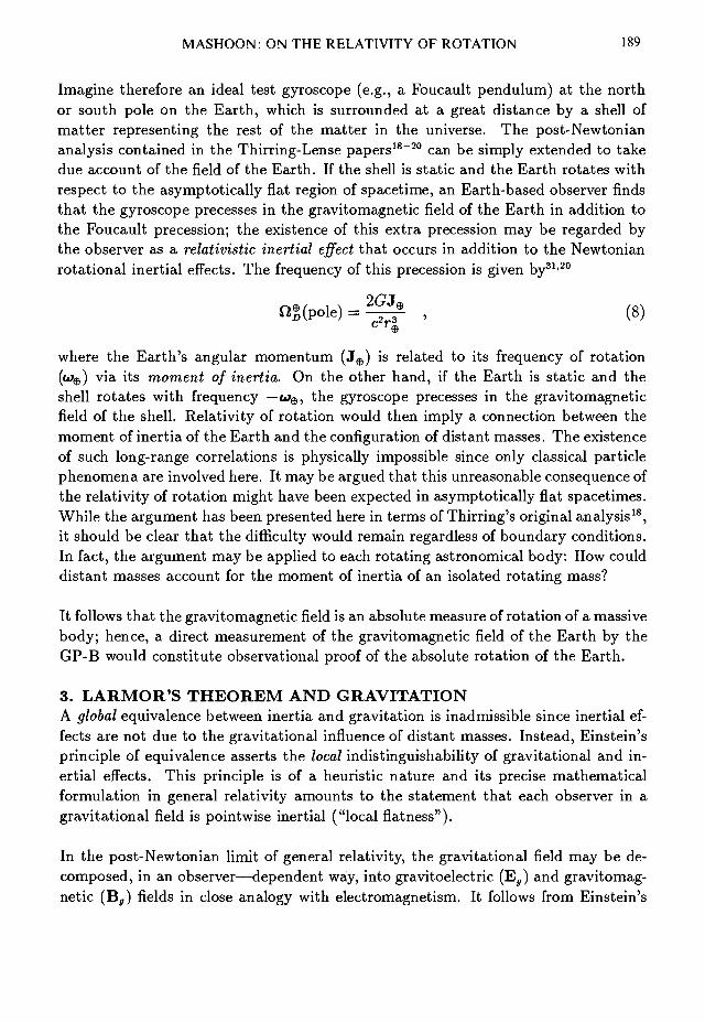
MASHOON: ON THE RELATIVITY OF ROTATION 189
Imagine therefore an ideal test gyroscope (e.g., a Foucault pendulum) at the northor south pole on the Earth, which is surrounded at a great distance by a shell ofmatter representing the rest of the matter in the universe. The post-Newtoniananalysis contained in the Thirring-Lense papers18"20 can be simply extended to takedue account of the field of the Earth. If the shell is static and the Earth rotates withrespect to the asymptotically flat region of spacetime, an Earth-based observer findsthat the gyroscope precesses in the gravitomagnetic field of the Earth in addition tothe Foucault precession; the existence of this extra precession may be regarded bythe observer as a relativistic inertial effect that occurs in addition to the Newtonianrotational inertial effects. The frequency of this precession is given by31'20
, (8)
where the Earth's angular momentum (J e) is related to its frequency of rotation(oje) via its moment of inertia. On the other hand, if the Earth is static and theshell rotates with frequency — a;e, the gyroscope precesses in the gravitomagneticfield of the shell. Relativity of rotation would then imply a connection between themoment of inertia of the Earth and the configuration of distant masses. The existenceof such long-range correlations is physically impossible since only classical particlephenomena are involved here. It may be argued that this unreasonable consequence ofthe relativity of rotation might have been expected in asymptotically flat spacetimes.While the argument has been presented here in terms of Thirring's original analysis18,it should be clear that the difficulty would remain regardless of boundary conditions.In fact, the argument may be applied to each rotating astronomical body: How coulddistant masses account for the moment of inertia of an isolated rotating mass?
It follows that the gravitomagnetic field is an absolute measure of rotation of a massivebody; hence, a direct measurement of the gravitomagnetic field of the Earth by theGP-B would constitute observational proof of the absolute rotation of the Earth.
3. LARMOR'S THEOREM AND GRAVITATIONA global equivalence between inertia and gravitation is inadmissible since inertial ef-fects are not due to the gravitational influence of distant masses. Instead, Einstein'sprinciple of equivalence asserts the local indistinguishability of gravitational and in-ertial effects. This principle is of a heuristic nature and its precise mathematicalformulation in general relativity amounts to the statement that each observer in agravitational field is pointwise inertial ("local flatness").
In the post-Newtonian limit of general relativity, the gravitational field may be de-composed, in an observer—dependent way, into gravitoelectric (E^) and gravitomag-netic (B^) fields in close analogy with electromagnetism. It follows from Einstein's

190 MASHOON: ON THE RELATIVITY OF ROTATION
principle of equivalence that these fields must be locally equivalent to inertial effects;the standard account of this principle12 corresponds to the local equivalence of thegravitoelectric field with a translational inertial acceleration. On the other hand, thegravitomagnetic field is locally equivalent to a rotational inertial effect. For instance,the gravitomagnetic field associated with a rotating mass is given by B^ = cClD,where the dragging frequency of the local inertial frames is
°» = §^ [3(r • J)r - r2J] . (9)
This amounts to a gravitational analog of Larmor's theorem32 since the gravitomag-netic field is proportional to the rotational dragging of the local inertial frames.
Larmor's theorem follows from a comparison of Newton's law of motion for a freeparticle in an accelerated reference system with the Lorentz force law. Local equiv-alence of inertial and electromagnetic effects can be established to first order in thefield strength for slowly varying fields and slowly moving charged particles with thesame q/m. The motion of a charged particle in an electromagnetic field is then lo-cally equivalent to the motion of a free particle with repsect to a reference framethat is accelerated with g L = <?E/ra and LJL = qH/2mc. The gravitational Larmortheorem has been described in a recent paper32; briefly, the analogy between the elec-tromagnetic and gravitational fields leads to the adoption of a gravitational chargeof magnitude ^(electr ic) = —m in the electric case and q g(magnetic) = —2m in themagnetic case. The latter convention is not surprising since a spin-2 field (gravity)has been approximated by a spin-1 field (electromagnetism). Moreover, in this con-vention the gravitational charges of the source of the field are assumed to be positiveand the corresponding test particle charges are assumed to be negative in order toaccount for the attraction of gravity. The universality of the gravitational interactionis reflected in the fact tha t for any test particle g L = —~E g and LJL = —~B g/c = — Q D.The gravitational field can therefore be characterized in terms of the translationaland rotational dragging of the local inertial frames.
The principle of equivalence is valid for classical particles and rays of radiation. Onthe basis of the gravitational Larmor theorem, deviations from the ray approxima-tion have been studied in order to elucidate the differential deflection of polarizedradiation in the gravitational field of a rotating mass.32 The same phenomenon maybe described for a particle, such as a thermal neutron33, through the interactionHamiltonian S • QDi where S is the particle spin. For the Earth, this amounts tohflf) ~ 10"29eV. Experiments have searched for a coupling of intrinsic spin with thegravitational field of the Earth34'35; however, it appears that some eight orders ofmagnitude improvement in sensitivity is required in order to measure the coupling ofintrinsic spin with the gravitomagnetic field of the Earth.
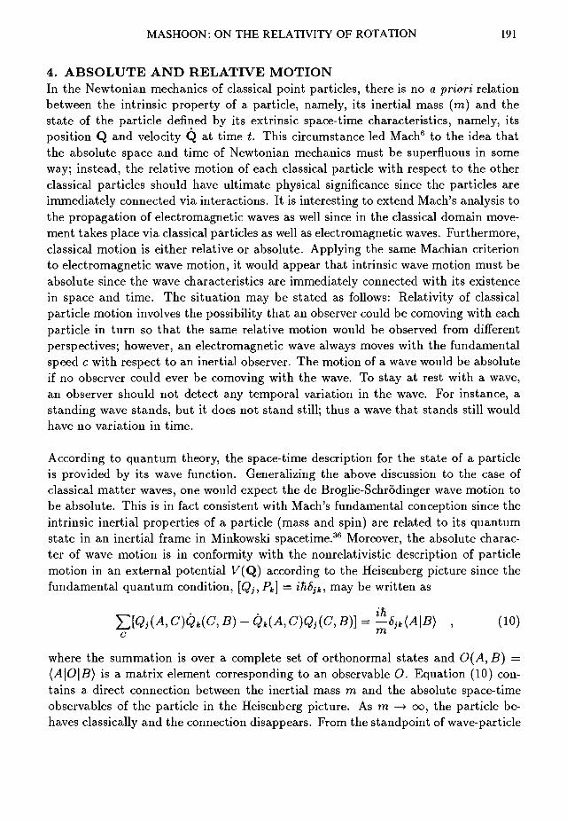
MASHOON: ON THE RELATIVITY OF ROTATION 191
4. ABSOLUTE AND RELATIVE MOTIONIn the Newtonian mechanics of classical point particles, there is no a priori relationbetween the intrinsic property of a particle, namely, its inertial mass (ra) and thestate of the particle defined by its extrinsic space-time characteristics, namely, itsposition Q and velocity Q at time t. This circumstance led Mach6 to the idea thatthe absolute space and time of Newtonian mechanics must be superfluous in someway; instead, the relative motion of each classical particle with respect to the otherclassical particles should have ultimate physical significance since the particles areimmediately connected via interactions. It is interesting to extend Mach's analysis tothe propagation of electromagnetic waves as well since in the classical domain move-ment takes place via classical particles as well as electromagnetic waves. Furthermore,classical motion is either relative or absolute. Applying the same Machian criterionto electromagnetic wave motion, it would appear that intrinsic wave motion must beabsolute since the wave characteristics are immediately connected with its existencein space and time. The situation may be stated as follows: Relativity of classicalparticle motion involves the possibility that an observer could be comoving with eachparticle in turn so that the same relative motion would be observed from differentperspectives; however, an electromagnetic wave always moves with the fundamentalspeed c with respect to an inertial observer. The motion of a wave would be absoluteif no observer could ever be comoving with the wave. To stay at rest with a wave,an observer should not detect any temporal variation in the wave. For instance, astanding wave stands, but it does not stand still; thus a wave that stands still wouldhave no variation in time.
According to quantum theory, the space-time description for the state of a particleis provided by its wave function. Generalizing the above discussion to the case ofclassical matter waves, one would expect the de Broglie-Schrodinger wave motion tobe absolute. This is in fact consistent with Mach's fundamental conception since theintrinsic inertial properties of a particle (mass and spin) are related to its quantumstate in an inertial frame in Minkowski spacetime.36 Moreover, the absolute charac-ter of wave motion is in conformity with the nonrelativistic description of particlemotion in an external potential V(Q) according to the Heisenberg picture since thefundamental quantum condition, [QjjPk] = ihSjk*, may be written as
52[QM,C)Qk(C,B) - Qh(A,C)Qs(C,B)] = -6jk{A\B) , (10)c m
where the summation is over a complete set of orthonormal states and O(A, B) =(A|O|i?) is a matrix element corresponding to an observable O. Equation (10) con-tains a direct connection between the inertial mass m and the absolute space-timeobservables of the particle in the Heisenberg picture. As m —> oo, the particle be-haves classically and the connection disappears. From the standpoint of wave-particle

192 MASHOON: ON THE RELATIVITY OF ROTATION
duality, the wave aspect becomes negligible as m —> oo. Consider, for instance, thepassage of a free nonrelativistic particle (e.g., a thermal neutron) of mass m andspeed v « c through a slit of width D; the angle of divergence of the correspondingbeam due to diffraction is given by 6 ~ h/mvD. As m —* oo, 8 —> 0 and the classical(i.e., non-quantum) situation is approached so that the law of inertia is recovered inthe classical limit. The importance of the ratio %/m —> 0 in the derivation of thesemiclassical limit of quantum mechanics should be noted.37 Thus the applicationof Mach's basic insight to the quantum mechanics of a particle leads to a properjustification for the absolute space and time of Newtonian mechanics: To the extentthat the classical mechanics of macroscopic systems can be thought of as a limitingform of quantum theory, Heisenberg's generalization of Hamiltonian mechanics to thequantum domain vindicates Newton's absolute space and time. This circumstanceis a direct consequence of the nonlocality of a particle in the quantum theory: Atany given instant of time, the Schrodinger wave function must be normalized over allspace.
The relationship between the intrinsic properties of a system and its extrinsic space-time characteristics, in the sense of Mach's analysis, may be expressed through theexistence of spatial and temporal scales h/mc and h/mc2, respectively, associatedwith the system. The intrinsic spatial scale must be compared with other significantlength scales in the problem; for instance, it can be shown that if the system is astandard classical measuring device undergoing acceleration, the relevant accelerationlength must exceed h/mc. Therefore, the (translational or rotational) accelerationof the system cannot exceed a certain mass-dependent maximal proper acceleration.This notion is originally due to Caianiello.38 On the other hand, the intrinsic tem-poral scale—when compared with the definition of time in terms of the period ofelectromagnetic radiation emitted in a certain standard atomic transition—impliesan absolute s tandard of inertial mass. This concept as well as its metrological implica-tions has been discussed by Wignall.39 It should be pointed out here tha t the quantumof circulation, h/m, has been measured for helium-4 atoms in experiments involvingsuperfluid helium,40'41 and for superconducting electrons through a superconductingde Broglie wave interferometer.42
The classical particle picture leads to the relative motion of particles, while the clas-sical wave picture leads to the absolute motion of the waves; the motion of a par-ticle has classical manifestations in terms of absolute and relative motion in directcorrespondence with wave-particle duality.43 This viewpoint is in harmony with allavailable da ta as well as the standard extension of Lorentz invariance to acceleratedsystems and gravitational fields once such extension is confined to the eikonal regimein which the standard theory has been tested successfully thus far. Only a beginning

MASHOON: ON THE RELATIVITY OF ROTATION 193
has been made in attempting to incorporate these ideas in a consistent manner intothe physical theory;44 a complete synthesis remains a task for the future.
It appears from a preliminary analysis that such a complementarity of absolute andrelative motion can be properly formulated only in Minkowski spacetime. It is ex-pected that when wave phenomena are treated in the eikonal approximation withinsuch a theory, the spacetime would appear to have an effective Riemannian curvature.In this way, contact could be established with the observational data that accountfor the success of general relativity. Thus the standard theory would be valid oncephenomena involving classical particles and rays of radiation are only taken into ac-count; beyond this approximation, new gravitational phenomena are expected whichhave not been explored as yet. Cosmology is based on the reception of null raysfrom cosmic sources; thus cosmological data—which can be interpreted according togeneral relativity—may indicate that our world is spatially open or closed. Eitherpossibility should then have an interpretation in terms of the effective curvature ofthe underlying Minkowski spacetime.
REFERENCES1. W. de Sitter, Mon. Not. Roy. Astron. Soc. 77, 155 (1916).2. C.W.F. Everitt et aln in Near Zero: Festschrift for William M. Fairbanks edited
by C.W.F. Everitt (Freeman, San Francisco, 1986).3. B. Mashhoon, H.J. Paik, and CM. Will, Phys. Rev. D39, 2825 (1989).4. V.B. Braginsky, A.G. Polnarev, and K.S. Thorne, Phys. Rev. Lett. 53, 863 (1984).5. B. Mashhoon, "On the Origin of Inertial Accelerations," UMC preprint (1991).6. E. Mach, The Science of Mechanics (Open Court, La Salle, 1960), ch. II, sec. VI
(n.b. part 11).7. B. Mashhoon, "Quantum Theory and the Origin of Inertia," UMC preprint (1992).8. N. Bohr and L. Rosenfeld, Mat.-fys. Medd. Dan. Vid. Selsk. 12, no. 8 (1933).9. B. Mashhoon, Phys. Lett. A143, 176 (1990).10. B. Mashhoon, Found. Phys. (Bergmann Festschrift) 15, 497 (1985).11. B. Mashhoon, Phys. Lett. A145, 147 (1990).12. A. Einstein, The Meaning of Relativity (Princeton University Press, Princeton,
1955).13. J.A. Wheeler, in Relativity, Groups and Topology, edited by B. DeWitt and C.
DeWitt (Gordon and Breach, New York, 1964).14. J. Isenberg, Found. Phys. (Wheeler Festschrift) 16, 651 (1986).15. J.A. Wheeler, Int. J. Mod. Phys. A 3, 2207 (1988).16. B. Mashhoon, in Quantum Gravity and Beyond: Essays in Honor of Louis Witten,
edited by F. Mansouri and J. Scanio (World Scientific, Singapore, 1993).17. M. Born, Einstein's Theory of Relativity (Dover, New York, 1962).

194 MASHOON: ON THE RELATIVITY OF ROTATION
18. H. Thirring, Phys. Z. 19, 33 (1918).19. J. Lense and H. Thirring, Phys. Z. 19, 156 (1918).20. B. Mashhoon, F.W. Hehl, and D.S. Theiss, Gen. Rel. Grav. 16, 711 (1984).21. D.R. Brill and J.M. Cohen, Phys. Rev. 143, 1011 (1966).22. J .M. Cohen and D.R. Brill, Nuovo Cimento 56B , 209 (1968).23. J .M. Cohen, Phys. Rev. 173, 1258 (1968).24. L. Lindblom and D.R. Brill, Phys. Rev. D10, 3151 (1974).25. B. Mashhoon, Phys. Rev. D l l , 2679 (1975).26. J.M. Cohen and W.J. Sarill, Nature 228, 849 (1970).27. J.M. Cohen, W.J . Sarill, and C.V. Vishveshwara, Nature 298, 829 (1982).28. H. Pfister and K.H. Braun, Class. Quantum Grav. 2, 909 (1985).29. H. Pfister and K.H. Braun, Class. Quantum Grav. 3 , 335 (1986).30. H. Pfister, Class. Quantum Grav. 6, 487 (1989).31. L.I. Schiff, Phys. Rev. Lett. 4, 216 (I960).32. B. Mashhoon, "On the Gravitational Analogue of Larmor's Theorem," Phys.
Lett . A, in press (1993).33. B. Mashhoon, Phys. Rev. Lett. 61 , 2639 (1988).34. D.J. Wineland and N.F. Ramsey, Phys. Rev. A5, 821 (1972).35. B.J. Venema et a/., Phys. Rev. Lett. 68, 135 (1992).36. E.P. Wigner, Annals of Math. 40, 149 (1939).37. P.S. Wesson, Space Sci. Rev. 59, 365 (1992).38. E.R. Caianiello, Riv. Nuovo Cimento 15, no.4 (1992).39. J .W.G. Wignall, Phys. Rev. Lett. 68, 5 (1992).40. W.F . Vinen, Proc. Roy. Soc. London A 260, 218 (1961).41. G.W. Rayfield and F. Reif, Phys. Rev. 136, A 1194 (1964).42. J .E. Zimmerman and J.E. Mercereau, Phys. Rev. Lett. 14, 887 (1965).43. B. Mashhoon, Phys. Lett. A126, 393 (1988).44. B. Mashhoon, "A Nonlocal Theory of Accelerated Observers," Phys. Rev. A, in
press (1993).

Recent Progress and Open Problems inLinearization Stability
V. Moncrief*
1. INTRODUCTIONOf the many influential contributions made by Dieter Brill to the mathematical devel-opment of general relativity, one of particular significance was his discovery togetherwith Stanley Deser, of the linearization stability problem for Einstein's equations [1].Brill and Deser showed that the Einstein equations are not always linearization stable(in a sense we shall define more precisely below) and they initiated the long (and stillcontinuing) technical program to deal with this problem when it arises.
Our aim in this article is not to review the extensive literature of positive resultson linearization stability but rather simply to introduce the reader to this subjectand then to discuss some recent research that has developed out of the study oflinearization stability problems. These latter include the relationship of linearizationstability questions to the problem of the Hamiltonian reduction of Einstein's equationsand lead one directly to the study of a number of recent results in pure Riemanniangeometry (e.g., the solution of the Yamabe problem by Schoen, Aubin, Trudingerand Yambe, the Gromov-Lawson results on the existence of metrics of positive scalarcurvature and the still unfinished classification problem for compact 3-manifolds).They also include a study of the quantum analogue of the linearization stabilityproblem which has been significantly advanced recently by the work of A. Higuchi onthe quantization of the first order gravitational perturbations of de Sitter space [2].
Many of the questions we shall discuss remain open (or at least partially so). Wehope this article may serve to stimulate further research in an interesting and subtlefield of relativity research.
2. THE LINEARIZATION STABILITY PROBLEM FOREINSTEIN'S EQUATIONS
The problem of linearization stability begins with the remarkable observation that,for certain given "background" Einstein spacetimes, there are some solutions of the
*Department of Physics, Yale University, 217 Prospect Street, New Haven, Connecticut 06511
195

196 MONCRIEF: PROGRESS IN LINEARIZATION STABILITY
associated linearized equations which cannot possibly be tangent to any differentiablecurves of exact solutions. In other words some solutions of the linearized equationsare "spurious" and should not be taken as first order approximations to nearby ex-act solutions. Furthermore one knows that , when such spurious solutions exist, thecomplementary non-spurious solutions do not form a linear space (even though theysatisfy a linear equation) but must be constrained to obey a certain second ordercondition.
Fortunately one now knows to a large extent when to expect such linearization in-stabilities (by which we mean the existence of spurious solutions of the linearizedequations) and what they signify about the space of exact solutions which one isat tempting to approximate by linearization. For simplicity we shall discuss only thecase of vacuum spacetimes having compact Cauchy surfaces and admitting at leastone such surface of constant mean curvature. It is important to keep in mind thecompactness assumption since results for non-compact (say asymptotically flat) hy-persurfaces are in general quite different [3]. Whereas the compactness assumption iscrucial, we have excluded material sources mostly for simplicity. Many of the resultswe shall describe extend naturally to the case of the Einstein-Maxwell or Einstein-Yang-Mills equations for example [4, 5].
Let M be a compact, orientable 3-manifold and let {<7,TT} be the usual HamiltonianCauchy data defined on M for a vacuum solution of Einstein's equations. This datais subject to the Einstein constraint equations which we shall abbreviate as
$(g,ir) = {H(g,*),-2 6-ir} = 0 (1)
where W(<7,7r) is the Hamiltonian constraint and — 2 8 • n the momentum constraint(a scalar density and one-form density respectively). Let M, formally denote the setof smooth Riemannian metrics on M and let T*M. denote its "cotangent bundle"consisting of the smooth pairs {<7,TT}. For simplicity we shall not here enter into thedetails of natural choices of function spaces for these quantities. Equation (1) definesthe constraint subset C of T*Ai
C = {{g,w)eT*M\$(g,n) = O}. (2)
The linearization stability problem hinges on the structure of the constraint set Cand its failure to be globally a manifold. At regular points (go^o) (which fortunatelyare generic) where C is a manifold, the tangent space to C is given by the kernel ofthe linearized constraint operator D$(gOJ7ro) and each solution (h,p) € T(gOino)T*Aiof
iro)-(h,p) = Q (3)
is indeed tangent to a curve lying entirely in C. The Einstein evolution equationsproduce no further complications and thus the solution of the full set of linearized

MONCRIEF: PROGRESS IN LINEARIZATION STABILITY 197
equations generated by such Cauchy data (h, p) is tangent to a curve of exact solu-tions.
Fischer and Marsden [6, 7] gave a precise formulation and proof of the above remarksand showed that (go,no) is a regular (manifold) point of C if D$(go,iro)*} the L2 -adjoint operator to D$(^o,7ro), has trivial kernel. The author showed [8, 9] that thekernel of D$(go,7ro)* corresponds precisely to (Cauchy data for) the global Killingfields admitted by the vacuum spacetime determined by the data (<7O,TTO). Thusif this spacetime has no non-trivial global Killing fields then (go^o) *s definitely aregular (manifold) point of C. The converse (that (go^o) is singular if Killing fieldsexist) is known to be true at least for spacetimes admitting a Cauchy hypersurfaceof constant mean (extrinsic) curvature and is believed to be true in any case. Toanalyze the singular points having ro = mean curvature = constant in more detailone uses the following characterization (due to Fischer and Marsden) of the kernel of
For vacuum Cauchy data of constant mean curvature the kernel of D$(go, KO)*is non-trivial if and only if either
(i) TTO == 0 and go is flat (in which case (1,0) lies in kernel), or
(ii) 3 a vector field X on M such that £x&> — ^X^o = 0 where Cx denotes the Liederivative with respect to X (in which case (0, X) lies in the kernel), or both.
In general the kernel, if non-trivial is spanned by a finite basis of elements of theabove two types (of which both may be present or either one absent).
The second order conditions upon the first order perturbations (h, p) of a singularpoint ((7o,?ro), which are now known to be both necessary and sufficient to excludespurious perturbations [10, 11, 12], can be written in the form
V(C,X)C kernel D$(go,iro)*. (4)
Here the first order Cauchy data (h, p) are assumed to obey the usual linearized con-straints, D$(gcn7ro)-(h,p\ = 0 (which are merely certain projections of the linearizedEinstein equations) and it is possible to show that the second order expressions £(C,X)are invariant with respect to the usual gauge transformations of the linearized the-ory. If the background data (^O,TTO), the perturbation data (h, p) and the Killingfield data (C, X) are all propagated by the relevant evolution equations it is alsopossible to show that the above second order conditions are conserved quantities and

198 MONCRIEF: PROGRESS IN LINEARIZATION STABILITY
thus independent of the Cauchy surface upon which they are first imposed. One canequivalently express conditions (4) as
L <<4> X . (D2 E i n s t e i n ^ ) • ((4)/i, (4)/i)) • (4)n > c*3S = 0 (5)
where (4)X, ^g and ^h are the Killing field, spacetime metric and spacetime pertur-bation respectively, ^4^n is the unit future pointing normal field to the hypersurfaceS and where D2 Einstein (^g) • (,) signifies the second variation of the Einsteintensor of ^g.
In summary one can say that the true linear approximation to Einstein's vacuumfield equation (about a background having compact Cauchy surfaces and non-trivialKilling symmetries) is not simply the usual linearized equation, D Einstein(^4^) •((4)/i) = 0, but instead this equation supplemented by the second order conditions((4) or equivalently (5)) described above. These conditions capture the fact that thespace of solutions is not a manifold at ^g but rather has conical singularities. Thusits associated "tangent space" is not the linear space that one expected but insteada linear space intersected with the second order conditions.
3. LINEARIZATION STABILITY AND THE SPACE OFCONFORMAL STRUCTURES OF A COMPACT 3-MANIFOLD
The issue of linearization stability arises in a new and interesting way when oneconsiders the global problem of Hamiltonian reduction of Einstein's equations forspacetimes having compact, orientable Cauchy hypersurfaces. Let M, as above, be acompact, orientable 3-manifold. In solving the constraints (one of the essential stepsin reduction) through the use of the standard conformal method [13] one notes thatonly the conformal class of a metric on M needs to be specified (together with atransverse traceless (t-t) symmetric 2-tensor field) in order to construct appropriateCauchy data. Lichnerowicz's equation determines the conformal factor which dis-tinguishes the true "physical" metric from all of its conformal equivalents. Thus anatural candidate for the reduced configuration space for Einstein's equations shouldbe the space of conformal structures on M [14].
One possible approach to realizing this space is to attempt to construct a submani-fold of the space A4(M) (of all smooth Riemannian metrics on M) which intersectseach conformal class transversally in precisely one point and upon which the groupV(M) (of smooth diffeomorphisms of M) acts naturally (through pull back of met-rics). A realization of the space of conformal structures could then be defined, modulotechnicalities which we shall not enter into here, as the quotient of the chosen sub-manifold by the given group action. In the model problem of Einstein's equations in2 + 1 dimensions this procedure leads (if V(M) is replaced by the subgroup £>0(M)

MONCRIEF: PROGRESS IN LINEARIZATION STABILITY 199
of diffeomorphisms isotopic to the identity) to the Teichmiiller space of the chosencompact 2-manifold as reduced configuration space ([15, 16]). In this case the cotan-gent bundle of Teichmiiller space plays the role of the reduced phase space and onecan identify, after making a suitable choice of time function, the Hamiltonian whichgenerates the dynamical flow induced from Einstein's equations. This Hamiltonianturns out to be simply the area function of the hypersurfaces of the chosen foliationexpressed in terms of the canonical Teichmiiller parameters and the time through thesolution of the constraints. In carrying out this program one finds that the sphereand the torus are exceptional whereas all the higher genus surfaces can be treatedin a uniform fashion. This happens because the sphere problem is vacuous in 2 + 1dimensions (there are no solutions having constant mean curvature Cauchy surfaces)whereas the reduced phase space for the torus has conical singularities (associatedprecisely with linearization instabilities of exceptional, static solutions). By contrast,linearization instabilities are absent for the higher genus surfaces and there are noobstructions to completing the program outlined above.
To generalize the above model to 3 + 1 dimensions one first needs to partition the com-pact 3-manifolds into various classes (analogous to the three classes mentioned above)corresponding to the different degrees of linearization instability that can occur. Thesimplest, and by far the largest, class of 3-manifolds to consider are those (like thehigher genus surfaces) which are incompatible with continuous isometries altogetherfor solutions of Einstein's equations. These have been identified (modulo the stillunproven Poincare conjecture) by A. Fischer and the author [17]. Most of these man-ifolds (a subset we call admissible manifolds) have the additional property that theyonly admit Riemannian metrics of the negative Yamabe class (i.e., metrics g which areglobally, uniquely conformal to metrics h having constant negative scalar curvature,R(h) = —1). It is easy to prove, for these admissible 3-manifolds, that the subspaceM-i(M) of the space of all Riemannian metrics M(M) on M satisfying the conditionR(g) = — 1 is in fact a smooth submanifold on which the group of diffeomorphismX>(M) of M acts naturally (by pullback of metrics). Modulo "technicalities" one candefine a space of conformal structures, T(M) = A/f_i(M)/P0(M), of M which playsa role completely analogous to the Teichmiiller space for higher genus surfaces inHamiltonian reduction. T(M) is the reduced configuration space and T*T(M) is thereduced phase space on which an appropriate Hamiltonian (the volume functional forthe chosen constant mean curvature foliation) generates the dynamical flow inducedfrom Einstein's equations. There are a number of interesting open mathematicalquestions concerning this definition of T(M). For example is T(M) globally a man-ifold or does it admit exceptional "orbifold-type"singularities due to the occurenceof non-trivial discrete isometries isotopic to the identity and does T(M), unlike theTeichmiiller space for a surface, have non-trivial "topology" or is it merely diffeo-morphic to an open ball in some Banach space? Orbifold singularities, even if theyoccur, will be complementary to an open dense set on which T(M) is a manifold butthis complication, if it arises, suggests that one use 7£(M) = A/(_i(M)/X>(M), the

200 MONCRIEF: PROGRESS IN LINEARIZATION STABILITY
analogue of Riemann moduli space, instead of T(M), the analogue of Teichmiillerspace, as reduced configuration space if the later choice has not successfully avoided(as it does in 2 + 1 dimensions) the orbifold singular points. These questions are achallenge for future research.
The question we wish to address here however is how can one generalize this picturefor reduction beyond the admissible manifolds to include all manifolds which topo-logically exclude linearization instabilities? According to the results in [17] (whichassume the Poincare conjecture and a conjecture that the only free finite group ac-tions on S are the standard orthogonal free actions of finite subgroups of SO(4))one finds that any manifold of the form
M * ss/ri#...#s3/r,#(s2 x s V . . . # ( s 2 x sx)P (6)where each I \ is a finite subgroup of SO(4) acting orthogonally on S 3 and whereq > 1 and q + r > 2 (so that these manifolds are necessarily composite rather thanprime) is not admissible (since it always admits metrics of the positive Yamabe class)but nevertheless (provided at least one of the Sz/T{ is not a lens space) excludessolutions of Einstein's vacuum field equations with continuous isometry groups (andCauchy surfaces of constant mean curvature). Furthermore it seems likely (thoughnot yet proven) that every manifold with these properties is of the above type (itremains to be shown that a manifold which admits non-trivial SO(2) actions alwaysadmits SO(2)-invariant Cauchy data). If the Poincare conjecture or the algebraicconjecture mentioned above should prove to be false then it is possible that a largerset of manifolds could have the properties described though little seems yet to beknown about the possible Yamabe classes admitted by such hypothetical counter-examples.
Any manifold of the type listed above admits metrics of all three Yamabe types. Thusone cannot hope to find a unique representative of every conformal class by imposinga condition such as R(g) = — 1 on the scalar curvature. This worked for admissiblemanifolds (as for the higher genus surfaces) only because these manifolds excludedmetrics of the positive and zero Yamabe classes altogether. One could perhaps try toreplace this with the condition that R(g) = constant together with the normalization(to freeze out constant conformal transformations) volg(M) = 1 where volg(NL) isthe Riemannian volume of (M,#). The problem however is that even though, thanksto the resolution of the Yamabe problem by Schoen, Aubin, Trudinger and Yamabe[18], every metric on M is globally conformal to one of constant scalar curvature andfixed volume, the conformal factor is not in general unique for metrics of the positiveYamabe class.
One source of non-uniqueness arises when g admits non-trivial, continuous, conformalisometries. Pulling back g by such a conformal isometry leaves the scalar curvatureconstant but sends g to an inequivalent element of the same conformal class. Atheorem of Obata however shows that, except for the case of the standard sphere,

MONCRIEF: PROGRESS IN LINEARIZATION STABILITY 201
the conformal isometry group of a compact, orientable Riemannian manifold (M,g)is always a subgroup of the isometry group of some conformally related manifold(M,/9g) [19]. But the manifolds listed above do not admit any SO(2) actions andso cannot admit metrics with continuous conformal isometries. Thus one source ofnon-uniqueness for the solution of the Yamabe problem has been excluded by ourpurely "topological" restriction on the choice of M. This however is not sufficient torender the choice of conformal representative unique.
To have any hope of making a unique choice of conformal representative one needs tointroduce a further condition such as, for example, requiring the metric in question tominimize the value of the Yamabe functional. If this minimal choice (which exists byvirtue of the solution of the Yamabe problem) is unique for the manifolds of interestwe can choose it as our representative from each conformal class. Thus one wouldbe led to consider the subspace of metrics of fixed volume, constant scalar curvatureand minimal value (within each conformal class) of the Yamabe functional (which infact already implies constancy of the scalar curvature). This space, if it proves tobe a manifold, might be chosen to play a role analogous to that of A4_i(M) in theadmissible cases described above.
The question however of whether a condition such as R(g) = constant (together witha volume normalization) determines a smooth submanifold of the space A4(M) is aninteresting problem in pure differential geometry [20, 21]. One can show that g is aregular (manifold) point of this space provided the equation (which represents theX2-adjoint of the derivative of the map which sends a metric to its scalar curvature)
- gAC + Hess C-C Ric(g) = 0 (7)
(where Ric(g) is the Ricci tensor of g and A and Hess are its Laplacian and Hessianoperators) admits only the trivial solution C = 0. Examples such as the standardsphere however are known for which this equation has non-trivial solutions. In fact allorientable conformally flat manifolds for which this equation has non-trivial solutionsare known, thanks to work by 0 . Kobayashi [22] and J. Lafontaine [23]. Aside fromthe sphere however all compact, orientable, conformally flat 3-manifolds of this typeare Riemannian products or warped products of the standard 2-sphere and the circle.Neither the 3-sphere nor S2 x S1 is of interest at the moment however since thesemanifolds always admit solutions of Einstein's equations with continuous isometries.
It seems conceivable therefore that, for the manifolds listed above, the equation R(g)= constant (supplemented by the volume normalization and the minimizing conditionon the Yamabe functional which as we noted implies the constancy of R(g)) doeslead to a smooth submanifold of A4(M) consisting of a unique representative fromeach conformal class. Since X>0(M) acts on this space one could take its quotientwith respect to this action and define a reduced configuration space by close analogywith the approach for admissible manifolds described above. Much analytical work

202 MONCRIEF: PROGRESS IN LINEARIZATION STABILITY
would be needed to justify this proposal but fortunately the question of how thespace of metrics having constant scalar curvature branches at points of bifurcationfor the solutions of Yamabe's problem is an important topic of recent research inpure Riemannian geometry [24]. It seems likely that advances in this pure geometryproblem will have immediate application to the reduction problem for Einstein'sequations.
What has the above got to do with linearization instability given that the manifoldsin question were chosen just so as to avoid the possibility of any such instabilities? Ananswer begins to emerge if we note that the equation R(g) = A = constant, whichappears in the approach to reduction described above, also arises in a completelydifferent context in general relativity:
Initial data (#,0) satisfying R(g) = A = constant on an arbitrary com-pact, orient able 3-manifold M are solutions of the constraints for a time-symmetric initial Cauchy surface in the presence of a cosmological constantA. The associated criterion for the absence of linearization instabilitiesis that Cx9 = 0 —» X = 0 (to exclude space-like isometries) and that-gAC + Hess C -C Ric(g) = 0 -> C = 0 (to exclude timelike or boostisometries).
In other words the question of whether Equation (7) admits non-trivial solutions isdirectly connected with the question of existence of linearization instabilities for theEinstein equations in the presence of a cosmological constant. Recognizing this onecan, for example, appeal to the results of Kobayashi and Lafontaine to characterizeall compact, conformally flat, time symmetric Cauchy data for a solution of Einstein'sequations with cosmological constant A and a boost Killing field [25]. These includethe de Sitter solution of course but also a family of solutions defined over Riemannianproducts and warped products of the circle and standard 2-sphere. The branchingsof the solution set for the pure geometry problem R(g) = A = constant are directlyrelated to the branchings of the space of solutions of the constraint equations for thespecial case of time symmetric data and a cosmological constant A. The existence ofsuch branching signals the presence of boost type Killing fields in the correspondingspacetimes.
That solutions of Equation (7) imply boost rather than merely timelike Killing fieldswhen A is non zero follows from taking the trace of this equation which gives 2AC =—AC. Integrating this result over (M, g) one easily finds that any non zero solutionmust change sign somewhere on M. This corresponds to the Killing field with normalprojection C changing from future directed timelike to past directed timelike in someregion of the initial surface. For the special case of the standard sphere (which givesrise to de Sitter spacetime) the four independent solutions of Equation (7) are com-prised of the four independent first order spherical harmonics and these correspondto the four boost Killing fields of de Sitter space.

MONCRIEF: PROGRESS IN LINEARIZATION STABILITY 203
4. QUANTUM ASPECTS OF LINEARIZATION STABIL-ITY
Lacking a well defined quantization of Einstein's equations we cannot expect to makerigorous statements about the quantum analogue (if there is one) of the linearizationstability problem. Since the source of the classical instabilities was the failure ofthe constraint set (and thus the reduced phase space) to be globally a manifold, itseems plausible that any successful approach to quantization would have to take thissignificant geometrical feature of the classical dynamics into account.
How should one quantize constrained systems whose constraint sets are not globallymanifolds? In the absense of a satisfactory general answer to this question one can askthe simpler question of how should one quantize the first order perturbations of someclassical "background" solution, in the case of general relativity, a classical Einsteinspace time? For simplicity assume the background is a vacuum metric ^g definedon M x R with M compact and that this spacetimes admits a foliation by Cauchyhypersurfaces of constant mean curvature. If (M/4) <gr) admits no global Killing sym-metries the issue of linearization instabilities does not arise and the quantization offirst order perturbations is, in principle, comparatively straightforward.
If Killing symmetries are present however then one must somehow impose a quantumanalogue to the second order conditions described in section II. Otherwise one couldconstruct "coherent states" representing essentially classical fluctuations about thebackground which violate the classical second order conditions (i.e., which correspondto spurious perturbations). The proposed quantization would then fail to have theproper classical limit and thus violate the elementary correspondence principle. Thusit seems clear that one needs to impose a quantum analogue of the second orderconditions.
These conditions are, as we saw, nothing more than certain projections of the con-straint equations expanded out to second order about the background. The particularprojections taken are uniquely characterized by the fact that they are independentof the second order perturbations (which we are not yet attempting to quantize) anddepend (quadratically) only upon the first order perturbations. These second orderconstraints supplement the usual linearized constraints which must of course also beimposed at the quantum level.
Formally one often thinks, following Dirac, of imposing constraints as linear restric-tions upon the space of physical states. One constructs operator analogues of theconstraints (here both first and second order) and requires the physical states to beannihilated by these constraint operators. This is a consistent procedure as longas there are no "anomalies" in the quantum commutator algebra of the constraints.There are no ordering ambiguities in the ordering of the linearized constraints and itis easy to verify that their commutators, one with another, vanish identically provided
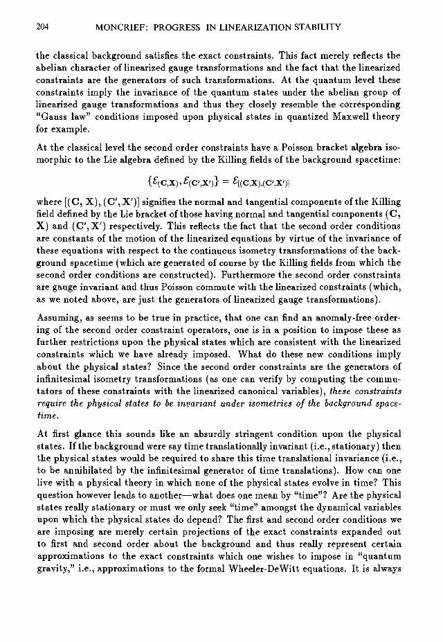
204 MONCRIEF: PROGRESS IN LINEARIZATION STABILITY
the classical background satisfies the exact constraints. This fact merely reflects theabelian character of linearized gauge transformations and the fact that the linearizedconstraints are the generators of such transformations. At the quantum level theseconstraints imply the invariance of the quantum states under the abelian group oflinearized gauge transformations and thus they closely resemble the corresponding"Gauss law" conditions imposed upon physical states in quantized Maxwell theoryfor example.
At the classical level the second order constraints have a Poisson bracket algebra iso-morphic to the Lie algebra defined by the Killing fields of the background spacetime:
where [(C, X), (C',X')] signifies the normal and tangential components of the Killingfield defined by the Lie bracket of those having normal and tangential components (C,X) and (C',X') respectively. This reflects the fact that the second order conditionsare constants of the motion of the linearized equations by virtue of the invariance ofthese equations with respect to the continuous isometry transformations of the back-ground spacetime (which are generated of course by the Killing fields from which thesecond order conditions are constructed). Furthermore the second order constraintsare gauge invariant and thus Poisson commute with the linearized constraints (which,as we noted above, are just the generators of linearized gauge transformations).
Assuming, as seems to be true in practice, that one can find an anomaly-free order-ing of the second order constraint operators, one is in a position to impose these asfurther restrictions upon the physical states which are consistent with the linearizedconstraints which we have already imposed. What do these new conditions implyabout the physical states? Since the second order constraints are the generators ofinfinitesimal isometry transformations (as one can verify by computing the commu-tators of these constraints with the linearized canonical variables), these constraintsrequire the physical states to be invariant under isometries of the background space-time.
At first glance this sounds like an absurdly stringent condition upon the physicalstates. If the background were say time translationally invariant (i.e., stationary) thenthe physical states would be required to share this time translational invariance (i.e.,to be annihilated by the infinitesimal generator of time translations). How can onelive with a physical theory in which none of the physical states evolve in time? Thisquestion however leads to another—what does one mean by "time"? Are the physicalstates really stationary or must we only seek "time" amongst the dynamical variablesupon which the physical states do depend? The first and second order conditions weare imposing are merely certain projections of the exact constraints expanded outto first and second order about the background and thus really represent certainapproximations to the exact constraints which one wishes to impose in "quantumgravity," i.e., approximations to the formal Wheeler-DeWitt equations. It is always

MONCRIEF: PROGRESS IN LINEARIZATION STABILITY 205
the case however, for quantization on spatially compact manifolds via the Wheeler-DeWitt approach, that one must seek an intrinsic time variable amongst the canonicalvariables in order to give dynamical meaning to the physical states. This is not easyto do in general and there is no universally accepted time function for this formalapproach to quantum gravity. Nevertheless one should not be surprised to see theneed for choosing an intrinsic time variable arising again in perturbation theory, atleast in those cases for which the background is stationary.
As noted above the only stationary vacuum background spacetimes having compactCauchy surfaces of constant mean curvature are in fact static and flat. The simplestare flat metrics on T 3 x R having one timelike and three spacelike commuting Killingfields. Quantization of the linearized perturbations of these models was considered bythe author who showed that one could choose an intrinsic time function (the perturbedspatial volume of the universe) and thereby give a natural dynamical interpretation tothe "time translationally invariant" Hilbert space of physical states [26]. The secondorder condition associated with the background timelike Killing field plays the roleof the basic dynamical "Wheeler-Dewitt equation" for the linearized quantum theoryand the physical states can be decomposed into "positive and negative frequencystates" corresponding to expanding or contracting universes respectively. If we imposethe super-selection rule of only admitting purely positive or purely negative frequencystates (i.e., of not mixing states describing perpetually expanding and perpetuallycontracting universes) then we can easily construct a conserved, positive definite innerproduct for physical states. After the linearized constraints have also been taken intoaccount, one can show that the resulting physical states consist of a "Fock-space" ofstates labeled by a complete set of transverse-traceless graviton quantum numberstogether with a finite set of variables describing purely homogeneous perturbations("infinite wavelength gravitons" [27]) and that these states evolve non-trivially withrespect to intrinsic time (i.e., perturbed volume).
That volume should make an acceptable time function for this problem is suggestedby the rigorous classical result that vacuum solutions on T 3 X R cannot admit amaximal hypersurface unless they are static and flat. Thus expanding solutions con-tinue to expand and contracting solutions continue to contract. This classical resultshould have a perturbative quantum analogue and does by virtue of our impositionof the second order condition described above. No state except the "Fock vacuum",which represents a trivial perturbation of the static background, can fail to representan expanding or collapsing universe. On the other hand, had we failed to impose thesecond order condition, imposing only the quantum analogues of the usual linearizedequations, we could easily have constructed coherent states representing large am-plitude, essentially classical gravitational waves which do not drive the universe intoa state of either expansion or collapse and which thus violate the elementary corre-spondence principle. Thus the second order condition, far from being the liabilityit first seemed, provides the linearized analogue of the Wheeler-DeWitt dynamical
206 MONCRIEF: PROGRESS IN LINEARIZATION STABILITY
equation and enforces consistency with the correspondence principle.
Actually, in this model, there are three more second order conditions (those asso-ciated with the spacelike Killing fields) which must also be imposed to completethe quantization of the linearized equations. They can be described equivalently asrequiring the space translational invariance of the physical states or of demandingthat the total spatial momentum of gravitons in the universe be zero. One shouldnot be distressed at this point to be dealing with a Hilbert space which (becauseof space translation invariance) cannot localize graviton energy with respect to thebackground spacetime. It is perfectly feasible to describe, within this framework,relative concentrations of say graviton energy even though the absolute location ofthis energy, relative to the background, is not determined. An example from theordinary non-relativistic quantum mechanics of many particle systems may help oneto see this. Suppose one considers a wave function for a many particle system whichis an eigenfunction of the total momentum with eigenvalue zero. Upon making theusual separation into relative and center of mass coordinates one easily sees that thewave function must be independent of the center of mass coordinates but can be anarbitrary function of the relative coordinates. Thus relative localization of particlesis perfectly well describable in a Hilbert space of zero total momentum states butabsolute localization (i.e., localization of the center of mass) is absent.
Of course there is no such zero momentum constraint to impose in ordinary quantummechanics but the analogy shows that all we "lose" in imposing such a constraint inthe quantization of linearized gravity is absolute localization of the center of massrelative to the background spacetime. On the other hand it is also clear that wecannot consistently think of "observers" within this framework who are localized rel-ative to the background spacetime. Observers could only be incorporated into thisframework by treating them as material sources coupled to gravity in the usual wayand quantized by a natural extension of the pure vacuum problem discussed above.This should perhaps not be surprising given the universality of the gravitational inter-action as captured by Einstein's strong equivalence principle. Nevertheless it seemssurprising to be forced to something resembling an Everett- Wheeler [28] interpreta-tion of quantum mechanics, in which observers are necessarily included as part of thequantum system under "observation" by considerations of linearization stability.
Perhaps the most fascinating application of the foregoing ideas is to the maximallysymmetric, spatially compact solution of Einstein's equations with a cosmologicalconstant—de Sitter spacetime. One can regard the cosmological constant as "put inby hand" or generated dynamically (as in inflationary models) but, in either case,the presence of ten Killing fields in the background leads to ten corresponding secondorder conditions to be imposed upon the physical states of the quantized linearizedtheory. These ten constraints require the full de Sitter invariance of all physical stateswhich again seems like an absurdly restrictive condition to impose in linearized quan-tum gravity. Indeed, the usual Fock space only admits one fully de Sitter invariant

MONCRIEF: PROGRESS IN LINEARIZATION STABILITY 207
state - the vacuum state. Our conclusion from this is not however that one mustmake do with only one physical state but rather that Fock space is not the rightHilbert space for the quantized perturbations of de Sitter space.
That it is possible to construct a Hilbert space consisting entirely of de Sitter invariantstates has been demonstrated by A. Higuchi [29] who showed, roughly speaking, thatone can define invariant states by "averaging non-invariant Fock space vectors overthe de Sitter group." Higuchi showed that one can define a new inner product suchthat these states, which would have infinite "norms" as computed formally in theoriginal Fock inner product, now all have finite inner products as computed usingthe new definition. Higuchi's Hilbert space is infinite dimensional and is presumablysufficiently rich in its structure to provide a "complete set of physical states" forthe quantized perturbations of de Sitter space. Because "time translations," definedrelative to the usual slicing of de Sitter space by standard spheres, are not isometriesthe Hamiltonian generating these translations is not constrained to annihilate thephysical states as a consequence of the second order conditions. Thus, unlike in theprevious example, there is no need to seek an intrinsic time function in order to givea dynamical interpretation to the quantum theory. The physical states do in generalevolve relative to the background.
In a quantum theory containing only invariant states the only meaningful "observ-ables" must themselves be de Sitter invariant. While one can define such observablesand compute their matrix elements in the linearized theory much as in conventionalquantum mechanics, there is the serious open problem of extending this formalism,in principle at least, to include higher order corrections. One must expect to face allthe usual questions associated with the non-renormalizability of the "quantized Ein-stein equations" as well as confront new ones associated with the necessity of workingwith a non conventional Hilbert space and extending the treatment of constraints,observables and dynamics to the higher order problem.
ACKNOWLEDGEMENT
This work was supported in part by NSF grants PHY-8903939, INT-9015153 andPHY-9201196 to Yale University.

208 MONCRIEF: PROGRESS IN LINEARIZATION STABILITY
REFERENCES
1. D. Brill and S. Deser, "Instability of Closed Spaces in General Relativity,"Commun. Math. Phys. 32, 291-304 (1973).
2. A. Higuchi, "Quantum linearization instabilities of deSitter spacetime," Class.Quantum Grav. 8, Part I: 1961-1981, Part II: 1983-2004, Part III: 2005-2021(1991).
3. See for example the discussion in "Local linearization stability" by D. Brill, 0 .Reula and B. Schmidt in J. Math. Phys. 28, 1844-1847 (1987) and referencescited therein.
4. J. Arms, "Linearization Stability of the Einstein-Maxwell System," J. Math.Phys. 18, 830-833 (1977).
5. J. Arms, J. Marsden and V. Moncrief, "The Structure of the Space of Solutionsof Einstein's Equations II. Several Killing Fields and the Einstein-Yang-MillsEquations," Ann. Phys. 144, 81-106 (1982).
6. A. Fischer and J. Marsden, Bui. Am. Math. Soc. 79, 997-1003. (1973) andProc. Symp. Pure Math., Am. Math. Soc. 27, Part 2, 219-263 (1975).
7. For a recent review see also the article by A. Fischer and J. Marsden in GeneralRelativity ed. S.W. Hawking and W. Israel (Cambridge, 1979).
8. V. Moncrief, "Space-time symmetries and linearization stability of the Einsteinequations. I," J. Math. Phys. 16, 493-498 (1975).
9. V. Moncrief, "Space-time symmetries and linearization stability of the Einsteinequations. II," / . Math. Phys. 17, 1893-1902 (1976).
10. This issue is treated by J. Arms, J. Marsden and V. Moncrief in Ann. Phys.144, 81-106 (1982) as well as in the following two references.
11. J. Arms, J. Marsden and V. Moncrief, Commun. Math. Phys. 78, 445-478(1981).
12. A. Fischer, J. Marsden and V. Moncrief, Ann. Inst. Henri Poincare 33, 147-194(1980); see also the original references cited herein.
13. Y. Choquet-Bruhat and J. York, "The Cauchy Problem" in General Relativityand Gravitation ed. A. Held (Plenum, New York, 1980).
14. See, for example, "The manifold of conformally equivalent metrics" by A. Fis-cher and J. Marsden, Can. J. Math. 29, 193-209 (1977).

MONCRIEF: PROGRESS IN LINEARIZATION STABILITY 209
15. V. Moncrief, "Reduction of the Einstein Equations in 2 + 1 Dimensions to aHamiltonian System over Teichmuller Space," J. Math. Phys. 30, 2907-2914(1989).
16. V. Moncrief, "How solvable is (2 + l)-dimensional Einstein gravity?", J. Math.Phys. 31, 2978-2982 (1990).
17. See the article "Recent advances in ADM reduction" by V. Moncrief in thecompanion volume dedicated to C. W. Misner.
18. For a recent treatment, which includes references to the original articles, seeJ. Lee and T. Parker, "The Yamabe Problem," Bull. Amer. Math. Soc. 17,37-81 (1987).
19. M. Obata, J. Math. Soc. Japan 14, 333-340 (1962).
20. See for example the discussion in chapter 4 of Einstein Manifolds by A. Besse(Springer-Verlag, 1987).
21. For a resolution of this problem in the special case of conformally flat Rieman-nian manifolds see Refs. [22] and [23] below.
22. O. Kobayashi, J. Math. Soc. Japan 34, 665-675 (1982).
23. J. Lafontaine, J. Math. Pure Appl 62, 63-72 (1983).
24. For a discussion of recent developments on this problem see the article by R.Schoen in Differential Geometry ed. B. Lawson and K. Tenenblat (LongmanScientific & Technical, 1991).
25. V. Moncrief, Class. Quantum Grav. 9, 2515-20 (1992).
26. V. Moncrief, Phys. Rev. D 18, 983-989 (1978).
27. The natural splitting of the transverse-traceless perturbations into spatialy ho-mogeneous modes and their Z2-orthogonal complement was not carried out inRef. [26] but can easily be obtained by a straightforward refinement of thedecomposition given therein; see Ref. [29] for details.
28. See, for example, The Many-Worlds Interpretation of Quantum Mechanics, B.S. DeWitt and N. Graham, eds. (Princeton Univ. Press, Princeton, 1973).
29. for a detailed treatment of the simpler problem of quantizing perturbations ofthe static, flat spacetime with toroidal spatial topology see A. Higuchi, Class.Quantum Grav. 8, 2023-2034 (1991).

Brill WavesNIALL 6 MURCHADHA
Physics Department, University College, Cork, Ireland
AbstractBrill waves are the simplest (non-trivial) solutions to the vacuum constraints of gen-eral relativity. They are also rich enough in structure to allow us believe that theycapture, at least in part, the generic properties of solutions of the Einstein equa-tions. As such, they deserve the closest attention. This article illustrates this pointby showing how Brill waves can be used to investigate the structure of conformalsuperspace.
1 INTRODUCTIONFrom time to time I amuse myself by mentally assembling a list of articles I wouldlike to have written. The candidates for this list have to satisfy a number of criteria.Naturally, they have to be both important and interesting to me. Equally, they haveto contain results that I can convince myself, however unreasonably, that I couldhave obtained. Every time I make my list I am struck again by the number ofarticles by Dieter Brill appearing on it. At first glance, this is explained by the largeoverlap between our interests. In reality, however, the explanation is to be found byconsidering the kind of article that Dieter has written over the years and the way inwhich he manages to convey major insights in a deceptively simple fashion. In thiswork I wish to return to an article that has a permanent place on my list, the famousBrill waves, and show how some of the the earliest work that Dieter did in generalrelativity continues to offer valuable insight a third of a century later.
2 BRILLIn his thesis (Brill, 1959) Dieter Brill considered axisymmetric, moment-of-time-symmetry, vacuum initial data for the Einstein equations.The starting point is anaxially symmetric three-metric of the following form
g = e2Aq(dp2 + dz2) + p2d02, (1)
where A is a constant and q is an (almost) arbitrary function of p and z. We onlyrequire that it satisfy q = qp = 0 along the z-axis, that it decay fairly rapidly atinfinity (faster than 1/r) and that it be reasonably differentiable.
This metric g is to be conformally transformed to a metric g = <f>4g so that the metricg has vanishing scalar curvature, so as to satisfy the moment-of-time-symmetry initial
210

6 MURCHADHA: BRILL WAVES 211
value constraint of the Einstein equations. This is equivalent to seeking a positivesolution </> to
8 V ^ - R(j> = 0, $ > 0, <j> -> 1 at oo, (2)
where R is the scalar curvature of g. It is easy to calculate
R=-2Ae-M'{q^ + qitt). (3)
It is important to notice that ^/g = pe2Aq so that
/ Rdv = / </gRd3x = —AA-K I p(q,pp + q>zz)dpdz
= -4ATT J[(pq,P - q),p + (pq,z)iZ]dpdz
= 0- (4)
To obtain the last line we have to use both the regularity along the axis and theasymptotic fallofF of q. This is a remarkably powerful result, in that it gave Brill thefirst positivity of energy result in General Relativity.
Let us assume that we obtain a regular solution to (2) (we will return to this issuein Section 3). The total energy, the ADM mass, is contained in the 1/r part of thephysical metric g. Since the base-metric g falls off faster than 1/r the mass must becontained in the 1/r part of the conformal factor </>. More precisely we get
Hence
2TTM = - I Va<j>dSa = - <fi -~TdSa (6)
' '^+{J^-]dv (7)
Notice that we use (4) in going from (7) to (8). The key (as yet) unresolved questionis: When can we solve (2)?
3 CANTOR AND BRILLThe next issue to be considered is what choices of q (or Aq) allow a regular solutionto (2). This question was first seriously discussed by Cantor and Brill (1981). Theyderived the following

212 6 MURCHADHA: BRILL WAVES
Theorem I (Cantor and Brill). There is a g conformally equivalent to a givenmetric g such that R(g) = 0 if and only if
|[8(V/)2 + R{g)f]dv > 0, (9)
for every f of compact support with f not identically 0.
Cantor and Brill further show that if R(g) is small (in a precise sense) then the Sobolevinequality may be used to guarantee inequality (9). The Sobolev inequality statesthat for any asymptotically flat Riemannian three-manifold there exists a positiveconstant S(g) such that
j(Vffdv>S(g)[Jrdv}^ (10)
for any / of compact support. Let us now use the Holder inequality on the secondterm in (9) to give
JR(g)f22dv < [J\R(g)\Uv}t[Jf6dv}$. (11)
Combining (10) and (11) shows that if
[f\R{g)\Uv]i<8S{g) (12)
then expression (9) must be positive for any / and a regular solution to (2) exists.
The Brill waves supply an obvious application of this result. Choose a metric of theform (1) with a fixed q but allow A to vary. It is clear from the expression (3) forthe scalar curvature that we can always find a small enough A (which can be eitherpositive or negative) to guarantee that (12) holds.
The next interesting property of the Brill waves is that, for a fixed g, one can alwaysfind a large enough value of A ( both positive and negative) such that inequality(9) cannot hold. We know that the scalar curvature integrates to zero. This meansthat it must have positive and negative regions. It is clear that we can always find anaxisymmetric function /+ which has support only on the positive regions of the scalarcurvature and another function /_ which has support only on the negative regions.This choice can be made independent of the value of A, We have that
jiVf+fdv = 2nj[(f^Y + (f+,.)*]pdpdz (13)
entirely independent of A. We also have
R{g)f\dv = 4*Af[-{q,pp + q,.,)]flpdpdz (14)

6 MURCHADHA: BRILL WAVES 213
where the integral on the right hand side of (14) is positive (from the choice of /+)and independent of A. Therefore, with this choice of test-function there exists anumber \A_\ given by
fittr + (u..
such that if A is large and negative, i.e., A < — |A_|, inequality (9) cannot hold. Asimilar bound, using /_, can be derived showing that there exists an \A+\ such thatif A > \A+\ (9) again breaks down.
This is not just a mathematical game, conformal transformations are the standardway of constructing solutions to the initial value constraints of General Relativity (0Murchadha and York, 1973) and for an interesting set of such data ('maximal' initialdata) a necessary and sufficient condition is that the metric be conformally trans-formable to one with zero scalar curvature. What we are doing, therefore, is tryingto map out conformal superspace 5; more precisely, we are trying to delineate theaxially symmetric subspace of conformal superspace (a so-called 'midisuperspace').The functions q(p, z) can be regarded as defining 'directions' in conformal superspacewith A acting as a 'distance' along each given ray. The 'point' A — 0 is flat space;there is an open interval around the origin on each ray which belongs to conformalsuperspace and each ray (after a finite 'distance') emerges from S.
We can even prove more; we can show that each ray passes only once out of 5.Given g, let us assume that we have passed out of 5, in other words we have an Ao
(assumed positive) such that inequality (9) does not hold. This means that thereexists a function fm such that
/[8(V/m)2 + R{g)fl]dv < 0. (16)
In other words,
y * p ) 2 + (fmiZf] - A0[(qtPP + q,zz)}fm)pdpdz < 0. (17)
The second term must be negative to counter the positive first term. It is clear that ifone increases A while holding fm and q fixed the inequality must worsen. Therefore,once a ray passes outside 5, it stays outside. In other words, (the axially symmetricpart of) S seems to be simply connected with convex boundary.
4 BEIG AND 6 MURCHADHAThe next question that needs be asked is what happens as one moves along such aray in S and approaches the critical value of A. This question has been addressed

214 6 MURCHADHA: BRILL WAVES
is a number of recent articles ( 0 Murchadha, 1987, 1989; Beig and 0 Murchadha,1991).
There exists an object analogous to the Sobolev constant, S(g), defined in equation(10), the conformal Sobolev or the Yamabe constant. The Yamabe constant is denned
^ 2 ^where the infimum is taken over all smooth functions of compact support. Thisobject has a number of interesting properties. It is a conformal invariant; it achievesits maximum value [equalling 3(^) 2 / 3 ] at (conformally) flat space (Schoen, 1984).Flat space is its only extremum.
One reason for introducing this concept here is that it allows a different formulationof Theorem I.
Theorem la. There is an asymptotically Hat metric g conformally equivalent to agiven metric g such that R(g) = 0 if and only if the Yamabe constant Y(g) of g ispositive.
One can immediately see this by comparing expressions (9) and (18).
The function that minimizes the Yamabe functional satisfies the non-linear equation
8V*<9 - R6 = -8A05, 9 -> 0 crfoo, (19)
where A is a constant that is proportional to the Yamabe constant. It equals theYamabe constant if 0 is normalized via
/ 0edv = 1.
I will use this normalization from now on. It can be shown (Schoen, 1984) that 0exists, is everywhere non-zero, and falls off at infinity like 1/r.
Let us now combine 0, the solution of eqn.(2), and 0, the solution of eqn.(18), usingthe Green identity
l a
Too= 8 j(6V2<t>-<t>V2e)dv
= f[OR<t> - 4>{Re - YO*)]dv
= Y fo5<f>dv.
(20)
(21)
(22)
(23)

6 MURCHADHA: BRILL WAVES 215
As Y approaches zero, both 9 itself, and the surface integral of 6 remain well-behaved.In particular, the 1/r part of 6 does not vanish in the limit. Therefore the surfaceintegral remains bounded away from zero. This means that the volume integral in(23) must blow up like 1/Y. Since 6 remains finite, (/> must become unboundedlylarge. In other words, <j) must blow up like 1/Y.
It is not enough that <j) blow up like a delta function at one point, it must becomelarge on an extended region so that the integral / 65(f>dv blows up like 1/Y. However,we know that (j) is not a random object, it satisfies a differential equation which forcesa broad blow-up on (j). We can make this more precise by returning to eqn.(2). Usingthe fact that yjg = pe2Aq, we find that (j) must satisfy
f + q,zz)<j) = 0, <j> > 0 , (j> - > 1 at o o , (24)
where V2 is the flat-space laplacian.
Let us consider the situation where q has compact support on some ball B. The scalarcurvature, i2, has the same compact support. Outside this region the manifold is flatand <f> satisfies V2
fð = 0. Hence the min-max principle tells us that the maximumof <f> must be achieved inside the ball B. Further, since <f> is positive and satisfiesa linear elliptic equation on the compact set B we can use the Harnack inequality(Gilbarg and Trudinger, 1983). This means that there exists a constant CB (whichwe can choose independent of A) such that
max </> = max</> < CB min</> < GB min</>. (25)B B SB
In other words, as the maximum of (j) increases inside in B, <f> everywhere in B getsdragged up with it. In particular, <fi on the boundary of B becomes large.
As A gets large, as Y gets small, we reach a point where max <j> > CB (the Harnackconstant). From that point on we have that rain6B(j) > 1. Outside B <f> satisfiesV2</> = 0. This means that the minimum and maximum of (f> occur on the boundariesof the set. Since <fr > 1 on 6B and (j) = 1 at infinity, the minimum must be at infinity.Returning to (5), (j> —> 1 + ^ , we can conclude that the constant M must be positive.This is a positive energy proof which is not as strong as the original Brill proof, itonly holds in the strong-field region, far away from flat space, as the Yamabe constantbecomes small. However, it has the advantage of working for a much larger class ofmetrics.
By analogy with electrostatics we can regard (j) (or rather £ = (j>— 1) as the potentialon and outside a (nonconducting) shell (SB). The potential on the shell is given andone solves for the potential outside. The ADM mass corresponds to the total charge
216 6 MURCHADHA: BRILL WAVES
that one has to distribute on the shell to give the specified potential distribution. Ifthe potential is everywhere positive on the shell, the charge must be positive.
If the shell were conducting, the potential on it would be constant. Now we can talkabout the capacitance C, the constant ratio between the 'charge' M and the potentialon the surface. The capacitance is a kind of Harnack constant because we have
C mini <M. (26)
C max£ > Af. (27)6B ^ — V '
These are easy to derive. Replacing a non-constant potential on SB by its minimum(maximum) value must decrease (increase) the charge while the decreased (increased)charge equals the capacitance multiplied by the potential. Since the capacitancedepends only on the size and shape of the surface, not on the charge, we immediatelysee that as min5S £ (or min^ <f>) increases , so will the ADM mass. If we incorporate(25), (26) and (27) together we can see that the mass grows linearly with <f>. Moreprecisely, we have
C— max <f) < M <C max </>, (28)
C min <f>< M < C.CB min </>. (29)B B
I can extract more information from (23). We have
Y f 0*<j>dv >Y f 0<f>dv > {Ymin<f>)[ 9*dv. (30)
The Harnack inequality (25) tells us that if K max <j> diverges as Y goes to zero, soalso will Y m\nB <t>- Eqn. (28) now tells us that Y f 0B<j)dv must become unboundedlylarge, which contradicts (23). Hence Fmax <f> remains bounded away from bothzero and infinity as Y goes to zero. In turn, this means that both Y min6B <f> andY max^ <j> remain finite and bounded away from zero as Y goes to zero. Finally, thismeans that the ADM mass blows up like 1/Y as Y goes to zero.
Not only does the monopole blow up like 1/Y, all the other multipoles behave in asimilar fashion. This allows us to show that a minimal two-surface must appear in theconformally transformed space if M becomes large enough. Let us consider a surfacewhich has coordinate radius r in the background (flat) space. The area of this surfacein the physical space is A = 47rr2</>4. AiV negative is equivalent to <j> + 2r</>r < 0. Theleading terms in </> are

6 MURCHADHA: BRILL WAVES 217
where Q is the quadrupole moment. Now we get
We need to find out if the right hand side of (32) can be negative. We know thatM will become large and positive but we have no control over Q except that theratio Q/M will remain bounded. A similar result holds for all the other multipolemoments. We can bound the third term by 10|(5|/r3. Let us evaluate (32) at r =M/4. This gives
• + * £ < l - 2 + « + ... (33)It is clear that as M becomes large (as Y becomes small) the third term (and allthe higher order terms) becomes small. This implies that the area of the surface inquestion reduces when it is pushed outwards. (Technically we should evaluate thechange in area along the outer normal rather than along the radial vector, however,the difference between the two becomes small as M and r become large.) This meansthat it is an outer trapped surface in the terminology of Penrose (1965). There is aminimal area surface outside all the trapped surfaces; this is the apparent horizon.
As M increases, the apparent horizon approximates more and more the sphericalsurface with radius r = M/2. The conformal factor on this surface equals 2, so theproper area of the apparent horizon approximates 16TTM2. The location of the ap-parent horizon moves outward (relative to the flat background) and its area increasesas M goes to infinity.
When M reaches infinity, when the horizon reaches infinity, when the Yamabe con-stant goes to zero, as A approaches the critical value, something catastrophic happens.The solution to (2) blows up and we can no longer construct an asymptotically flatmanifold with zero scalar curvature. On the other hand we have a solution to (19)with A = 0. This is a conformal factor that transforms the given base manifold intoa regular compact manifold with zero scalar curvature. Thus one can construct aclosed, vacuum cosmology at moment of time symmetry. If we increase A beyond thecritical value, we recover a finite solution to (2), but at the price of allowing </> < 0in a region. This is John Wheeler's 'Bag of Gold'.
5 WHEELERLet me move back in time. The earliest application I know of the Brill Wave solutionwas by John Wheeler in 1964. He considered eqn.(24) and brought his understandingof the Shrodinger equation to bear on it. He realised that it was just a scatteringproblem off a localized potential. The 'potential ' (R) averages to zero, but Wheelerrealized that the negative parts of the potential were much more important than

218 6 MURCHADHA: BRILL WAVES
the positive parts . He threw away the positive parts and considered only a negativepotential. He even further simplified the problem and considered the problem ofscattering off a negative spherical square well potential. He wrote down an analyticsolution to this problem.
Wheeler considered a spherically symmetric square well potential in flat space, i.e.,
u — —B, r < a
u = 0, r > a. (34)
It is easy to solve
V2ip - uip = 0 ip -» 1 at oo. (35)
The solution is
1 sin£1/2rb cos B^a
a1 +
r < a
So long as Bl/2a < TT/2, jp in (36) is well behaved. As B1/2a approaches TT/2, bothifc itself, and the coefficient of the 1/r part (the ADM mass equivalent) become un-boundedly large. Further, the surface on which ip — 2 (the analogue of the apparenthorizon) moves out towards infinity.
At the critical point (B1/2a = TT/2), ip ceases to exist. We now obtain a solution to arelated equation
V 2 ^ - wp = 0, tp -> 0 at oo. (37)
sin
r > a - ( 3 8 )
This is the equivalent of the Yamabe constant going to zero.
In retrospect, I am amazed how accurately this highly simplified model capturesthe behaviour of the actual situation. When the well is shallow, we have a regularscattering solution and the energy of the lowest eigenstate is positive. As the well isdeepened the energy of the lowest state moves down towards zero. As this happens,we get the phenomenon of resonant scattering, the scattering solution grows biggerand bigger. When the well is just deep enough to give us a zero energy bound state,

6 MURCHADHA: BRILL WAVES 219
the scattering state blows up and ceases to exist. If the well is made even deeper,the scattering solution reappears but now it is no longer everywhere positive, it hasa node. This pattern repeats itself as the energy of the next lowest energy stateapproaches zero, and so on.
The 1/r part of the scattering solution also blows up as one approaches the criticalpoint. If one approaches the critical point from the other side, where the scatteringsolution has a node, the coefficient of the 1/r term approaches — oo. This now allowsone to give a fairly nonsensical answer to a fairly unreasonable question: What is theenergy of a closed universe? My answer is zero, the average of +00 and —00!
We now have a fairly precise understanding of what happens as we pump up oneof the Brill waves; the Yamabe constant approaches zero for some finite value ofthe parameter A, the mass approaches +00 and an apparent horizon appears whichmoves out towards infinity. The horizon, as it moves outwards, becomes more andmore spherical. The breakdown of the system coincides with the horizon reachingspacelike infinity. At the critical point we get data which gives us a smooth compactmanifold, without boundary, with zero scalar curvature.
I would like to point out here that we have less understanding of what happens aswe further increase the factor A. Our only real guide is the Wheeler model. If this isvalid, the mass should drop to — 00 just on the other side (we would have initial datawith a naked singularity), the mass would build up again until it became positiveand then blow up to +00 as the eigenvalue of the first excited state approached zero,and so on. It would be nice to prove that this is (or is not) the correct picture.
The analysis given in Section 4 only deals with the situation when the Yamabeconstant is close to zero. Does it hold in general? In particular, if one takes aBrill wave and increase the constant does the mass increase monotonically, does theYamabe constant decrease monotonically? These are questions that are yet to beanswered.
An even more fundamental question: What happens as one approaches the boundaryof conformal superspace along a different direction, i.e., not by holding q fixed andincreasing A, but by changing ql I am unable to answer this question definitively, allI can say is that it is currently being investigated by numerical techniques.
6 ABRAHAMS, HEIDERICH, SHAPIRO AND TEUKOLSKYBrill waves have been used by the numerical relativity community from its earliestdays (e.g. Eppley, 1977) and this use has continued right up to the present. The

220 6 MURCHADHA: BRILL WAVES
standard approach (pioneered by Eppley) is to choose a metric of the form (1), withq chosen to be some analytic function. Equation (2) is then solved numerically to findthe conformal factor <j>. Finally, the 'physical' metric g — <fi4g is constructed. Eppleyshowed numerically that the overall structure described in the previous sections holdstrue. With a small scale factor A, equation (2) can be solved. As A increases, theconformal factor increases in the middle. Eventually a minimal surface (an apparenthorizon) appears in the physical space. Finally, at some finite value of A, the solutionto (2) blows up.
Recently, Abrahams, Heiderich, Shapiro and Teukolsky (1992) showed that this pic-ture of conformal superspace was grossly oversimplified. They chose as q the function
q = p2 exp[»(•—• + ^ - ) ] . (39)
Now, instead of holding q fixed in the traditional fashion, they varied q by reducingthe 'characteristic wavelength' Xp slowly while holding Xz fixed. Further, they keptchanging the scale factor A so that the ADM mass of the physical metric remainedat the constant value M = 1. They showed that the scale factor A grew rapidly,A oc X~2 as Ap —> 0. It is clear that for all values of Xp ^ 0,the base metric and thephysical metric exist and are regular, asymptotically flat, axially symmetric Rieman-nian metrics with positive Yamabe constant. However, both the base metric and thephysical metric become singular when Xp = 0. Most importantly, nowhere along thesequence do apparent horizons appear in the physical metric.
This analysis raises major questions about the simple description of conformal su-perspace obtained in Section 4 by holding q fixed and changing A. AHST are alsoprobing the boundary of conformal superspace and seem to have discovered that theboundary, in addition to smooth metrics with Y — 0, also contains singular metrics.
In the spirit of AHST, let me consider the following sequence of metrics
with
9A = T^ exP[~("TJ + £2)]- (41)
It is clear that, for some fixed, small (7, for each #A, as A —> 0, one can get a regularsolution to Eqn.(2). Further, the ADM mass along the sequence remains (more-or-less) constant and no apparent horizon appears.
Let me now make a (constant) coordinate transformation on each metric gx replacingp with Xp and z with Xz. This changes (40) to
frfz2) + p2d02], (42)

6 MURCHADHA: BRILL WAVES 221
with(p> + \7z% (43)
Now I conformally transform gx by dividing it by A2 to finally get
g'x' = e2Cq>(dp2 + dz2) + p2d02. (44)
This combination of coordinate and conformal transformations cannot change thevalue of the Yamabe constant. This means that we can still solve (2) for each g'x.However, the value of the ADM mass is not a conformal invariant; it picks up a factorA"1. Thus the new mass, instead of remaining constant, blows up as A —> 0.
When one looks at q'x, eqn.(43), it is clear that the limiting metric is no longersingular. However, it is still unpleasant, as it is no longer asymptotically flat. Thecz' dependence in q1 drops out and the metric becomes cylindrically symmetric ratherthan axially symmetric.
The ADM mass is measured with respect to some 'uni t ' (meters, lightyears, what-ever). This combination of coordinate transformation together with a conformaltransformation can be regarded as the equivalent of a change of units, and the valueof the ADM mass will change appropriately. Thus any relationship between the massand the Yamabe constant can only be valid in some very restrictive sense, one has to'fix the uni ts ' .
Let me return to the other feature that AHST observed, the absence of apparenthorizons. It does not mat ter whether one performs this combination of constantcoordinate and conformal transformations on the base space or on the physical space.Apparent horizons at moment-of-time-symmetry are equivalent to minimal 2-surfaces.Minimal 2-surfaces are stable under constant scalings. Therefore, if AHST find noapparent horizons neither will I, even though the mass blows up for the sequence Iconsider. This does not contradict the analysis in Section 4. In that section I assumedthe existence of an 'external ' region where the physical geometry was dominated bythe conformal factor. In the sequence of metrics considered here the support of thebase scalar curvature spreads ever outwards, preventing us from taking advantage ofthe increase of M.
It is not even clear what happens to the Yamabe constant in the limit A —> 0. All Ican say is that it will not pass through zero at any finite value of A. There is a hintin Wheeler 's spherically symmetric toy model that the Yamabe constant may remainnonzero, even in the limit.
Let us return to (36),but instead of considering a sequence in which J31/2a approachesTT/2, let us increase a and simultaneously scale down B so that Bl^2a remains constant

222 6 MURCHADHA: BRILL WAVES
(equal to, say, TT/4). NOW, the coefficient of the 1/r term becomes unboundedly large(it scales with a) . However, the value of i\) itself never becomes large, we find ip < \ /2holds true no mat ter how large a becomes. Hence we never obtain a surface on whichip = 2. Further, the limit a —> oo does not correspond to the appearance of a zeroenergy bound state, a solution to (37). Thus, the limit point that AHST investigatealmost certainly does not correspond to the Yamabe constant going to zero.
This trick, used by AHST, of scaling the sequence so that the mass remains constant,can also be implemented for the 'regular' sequences discussed in Section 4. Wheelerhad already realised this in 1964. There are three equivalent choices of scalings:(i) : Instead of letting the conformal factor <j> go to 1 at infinity, solve (2) with thecondition max</> = 1. This was the choice Wheeler made.(ii) : Retain (j) —* 1 at infinity, but multiply all the coordinates with the Yamabeconstant Y.(iii): Retain <j> —•» 1 at infinity, but divide all the coordinates by the ADM mass.
With each of these constant scalings, the appearance of minimal surfaces is uneffected.Now, however, as one moves along the sequence, as the minimal surface moves outto infinity, the area of the horizon shrinks to zero. When it pinches off at 'infinity',it really is at a finite proper distance from the middle. Further, it does so smoothly,we do not get a conical singularity, instead we get a regular closed manifold. Asone moves further along the sequence, into the region of negative Yamabe constant,I expect that this pinched off point moves back from infinity and develops into aconical singularity. Thus we get again an asymptotically flat manifold, but now onewith a naked singularity.
7 CONCLUSIONSWhat I have been calling conformal superspace, the space of asymptotically flat,Riemannian, 3-manifolds that can be conformally transformed into (asymptoticallyflat) regular manifolds with positive scalar curvature, is an interesting object. It isthe natural space one is left with if one, in a 3 + 1 analysis of the Einstein equations,factors out the Hamiltonian as well as the momentum constraints. If one does notwish to proceed this far, one can still think of it as an interesting subset of regularsuperspace, metrics on which we expect to find regular, classical solutions of theconstraints.
Conformal superspace, 5, consists of all asymptotically flat, smooth, Riemannianmetrics with positive Yamabe constant. The boundary of this space, the limit pointsof (smooth) sequences of metrics in S will, presumably, consist of metrics whichviolate one or other of the defining properties of S. In other words we expect to

6 MURCHADHA: BRILL WAVES 223
find metrics which are not asymptotically flat, metrics which are not smooth, metricswhich are not uniformly elliptic and metrics for which the Yamabe constant equalszero.
What understanding we have of such issues as the 'size' and 'shape' of conformalsuperspace has basically been gained by looking closely at the Brill waves. I amconvinced that yet more information can and will be extracted from them. In myintroduction I stated that they "offer valuable insight a third of a century later".I have every expectation that this will continue to hold true for another third of acentury.
AcknowledgementsI would like to acknowledge my debt to Bobby Beig, significant parts of this article arejust a recasting of our joint work. I would like to thank Edward Malec for criticallyreading the manuscript.
REFERENCESAbrahams, A., Heiderich, K., Shapiro, S. and Teukolsky, S. (1992), Phys. Rev. D46,1452-1463.Beig, R. and 6 Murchadha, N. (1991), Phys. Rev. Lett. 66, 2421-2424.Brill, D. (1959), Ann. Phys. (N.Y) 7, 466-467.Cantor, M. and Brill, D. (1981), Compositio Mathematica 43, 317-330.Eppley, K. (1977), Phys. Rev. D16, 1609-1614.Gilbarg, D. and Trudinger, N. (1983), Elliptic partial differential equations of secondorder (Springer, Berlin).0 Murchadha, N. and York, J. W. (1974), Phys. Rev. D10, 428-436.O Murchadha, N. (1987), Class. Quantum Grav. 4, 1609-1622.6 Murchadha, N. (1989), in Proceedings of the CM.A. Vol.19, edited by R. Bartnik(C.M.A., A.N.U., Canberra) 137-167.Schoen, R. (1984), J. Diff. Geom. 20, 479-495.Wheeler, J. A. (1964), in Relativity, Groups and Topology, edited by B. DeWitt andC. DeWitt (Gordon and Breach, New York) 408-431.

You Can't Get There from Here:Constraints on Topology ChangeKRISTIN SCHLEICH AND DONALD M. WITT
Department of Physics, University of British Columbia, Vancouver, BC V6T 1Z1
AbstractRecent studies of topology change and other topological effects have been typicallyinitiated by considering semiclassical amplitudes for the transition of interest. Suchamplitudes are constructed from riemannian or possibly complex solutions of theEinstein equations. This simple fact limits the possible transitions for a variety ofpossible matter sources. The case of riemannian solutions with strongly positivestress-energy is the most restrictive: no possible solution exists that mediates topol-ogy change between two or more boundary manifolds. Restrictions also exist forriemannian solutions with negative or indefinite stress-energy sources: all boundarymanifolds must admit a metric with nonnegative curvature. This condition stronglyrestricts the possible topologies of the boundary manifolds given that most manifoldsonly admit metrics with negative curvature. Finally, the ability to construct explicitexamples of topology changing instantons relies on the existence of a symmetry orsymmetries that simplify the relevant equations. It follows that initial data withsymmetry cannot give rise to a nonsymmetric solution of the Einstein equations.Moreover, analyticity properties of the Einstein equations strongly suggest that ingeneral, complex solutions encounter the same topological restrictions. Thus the pos-sibilities for topology change in the semiclassical limit are highly limited, indicatingthat detailed investigations of such effects should be carried out in terms of a moregeneral construction of quantum amplitudes.
1 INTRODUCTIONOne of the most striking features about the observed universe is that on distancescales ranging from fermis to megaparsecs its spatial topology is Euclidean. As thereare a multitude of solutions to the Einstein equations with R3 or S3 spatial topology,this observed feature is consistent with the classical dynamics of general relativity butis by no means required; one can show that all spatial topologies admit initial datasuitable for finite evolution under the Einstein equations. In fact, even particularlynice spacetimes such as homogeneous inflationary solutions can have complicatedspatial topologies [1]. Moreover, the topology of an initial data slice cannot changeunder such evolution. Thus, as topology change cannot occur by classical evolutionfrom an initial data set, any explanation of the spatial topology of the observed
224

SCHLEICH AND WITT: CONSTRAINTS ON TOPOLOGY CHANGE 225
universe must arise from its initial conditions, that is near its initial singularity. Asthe characteristic energy scales become large at this point, quantum fluctuations inboth the matter and the metric become important to the dynamics of the universe.Such quantum fluctuations violate the classical energy and causality conditions andcould lead to topology change. Therefore, it is natural to search for answers toissues concerning topology and topology change in terms of the quantum mechanicsof gravity.
A favorite starting point for addressing such issues has been to study the low energylimit of quantum amplitudes for gravity. Such semiclassical amplitudes are formedfrom the action of classical solutions of the appropriate Einstein equations. Ampli-tudes between two boundarys of the same topology are formed from the action ofclassical Lorentzian solutions corresponding to the evolution from the specified ini-tial geometry to the final geometry. However, amplitudes for two or more boundariesof different topologies cannot be formed from such solutions; instead they must beconstructed from the action of classical Euclidean, or possibly complex, solutions [2].Such amplitudes must satisfy certain boundary conditions whose generic form is thaton each boundary manifold S, both the extrinsic curvature and the normal deriva-tive of the matter fields vanish [3]. Thus the possibility for initial topologies and fortopology change are dictated in the low energy limit by the existence or non-existenceof such appropriately behaved Euclidean or complex solutions.
Only a few explicit topology changing Euclidean solutions are known [4, 5]; indeed oneof Dieter Brill's recent contributions to relativity has been in finding such solutions[6]. However, these few examples have played an important role in the study oftopology change and topological effects as they form the basis for other interestingarguments and calculations [7]. Understandably, such explicit examples of topologychange are hard to construct and are special in nature; the existence of some type ofsymmetry such as an isometry or conformal isometry is used to simplify the Einsteinequations into a tractable form. Therefore, as such solutions are not generic, it isinteresting to know what kind of restrictions there are on the existence and propertiesof topology changing solutions that do not necessarily have any symmetry.
The first restriction on the existence of such solutions is purely topological; mani-folds that lie in different cobordism classes cannot be boundaries of any mediatinginstanton. However, apart from this very weak restriction, additional constraints onthe existence of such solutions arise from an interesting interplay of geometry withtopology. This paper will discuss the possibilities for the existence of such instantonsin several cases. It will become apparent that such general topology changing solu-tions are actually rather hard to come by, even if negative or indefinite stress-energy

226 SCHLEICH AND WITT: CONSTRAINTS ON TOPOLOGY CHANGE
matter sources are allowed. In fact, the possibilities for topology change are highlyrestricted in the semiclassical limit. Finally, the assumption of symmetry furtherlimits the possible riemannian or complex solutions.
2 EUCLIDEAN INSTANTONS
2.1 Strongly Positive Stress-EnergyIt is useful to begin by discussing the case of Euclidean instantons with nonnega-tive Ricci tensor. Such instantons correspond to the Euclidean generalization of thefamiliar Lorentzian situation in which the matter satisfies the strong energy condi-tion, i.e. the spacetime has nonnegative Ricci tensor. Thus such solutions can beaptly described as having strongly positive Euclidean stress-energy. It can be proventhat such Euclidean solutions cannot produce topology changing instantons [8]. Thisresult is most readily illustrated for the case of compact instantons with vanishingextrinsic curvature on all boundaries. For this special class of instantons, the prooffollows from the following generalization of Bochner's theorem:
Theorem 1. Let Mn be a closed n-manifold with a riemannian metric such thatRab > 0. Then the universal cover ofMn, Mn = R* x Sn"fc where k = dim F ^ M " ; R)and Sn"fc is a simply connected manifold. Furthermore, the metric is a productg = f + h where f is a flat metric on R and h is a metric with Rab > 0 on £n~*.
First, note that the integer k is just the first betti number ijfM"). Next each non-trivial generator u of Hl corresponds uniquely to a harmonic 1-form a on Mn\ that isa = uj + d^y where 7 is a unique function on Mn. To show this recall that a is harmonicif ACT = (8d + d8)a = 0, where d is the exterior derivative and 6 is its dual in the L2
inner product of forms. Equivalently, a form is harmonic if and only if 8 a = 0 andda = 0. Therefore, in order for there to be a harmonic a corresponding to u>, bothduj + dd~f = 0 and 8u + Sdj = 0. The first equation is satisfied trivially, the secondrequires that there exist a unique function 7 such that 6d*y = —8u. If the exteriorderivative is represented by the anti-symmetrized covariant derivative of a form, then8 is the negative divergence with respect to the first index of the form. Hence, theequation for 7 is equivalently written as — V 27 = Vaa;a. Since Gauss' law impliesfMn 8UJ = 0, it follows that 8u> is orthogonal to the kernel of —V 2 in the L2(Mn)inner product. Hence, there exists a unique weak solution 7 on Mn. Finally, ellipticregularity theorems imply that this solution is a strong smooth solution. Therefore,given any nontrivial element of Hx(Mn) there is unique harmonic 1-form in Ti}{Mn)such that a = u + df. Hence V}(Mn) 2 Hl(Mn).
Next, observe that for any harmonic <r,
0 = / c-(6d + dS)a= I (-<rcVh(Vb<7c - V,a4) - acVcV"ah)dn (1)JMn JM" \ J

SCHLEICH AND WITT: CONSTRAINTS ON TOPOLOGY CHANGE 227
where d\i is the measure on the manifold Mn. Using the relation Va V6i;a — V6Vava =R*vd, (1) reduces to
0 = JMn ((Vhacf + <7aa"Ra^ d» (2)
after an integration by parts. If Rah is positive, the right hand side of (2) is positive.Therefore, by contradiction there must not exist any such harmonic form a and thusH1(Mn] R) = 0. If Rab is nonnegative then the right hand side of (2) can vanish if
Vaab = 0. aaahRab = 0 (3)
It follows directly that ah must be a Killing vector of constant length. Therefore foreach such harmonic form, Mn must locally be a product manifold or to be precise, theuniversal cover Mn must contain one copy of R. Moreover, the metric on the covercan be split using this Killing vector. Consequently if there are k such nontrivial1-forms, Mn = It* x Y,n~k where Sn~* is a simply connected manifold and its metricis a product g = f + h where / is a flat metric on IR* and h is the metric on En~*.Q.E.D.
If b1(Mn) ^ 0 then the above theorem implies that there is at least one zero eigenvalueof the Ricci curvature because the metric locally splits on Mn. Therefore, if Rah > 0for some riemannian metric on M n , it follows that bi(Mn) = 0. Thus the geometryand topology are closely linked for closed manifolds with nonnegative Ricci. Giventhe above theorem, the following result for compact Euclidean instantons can beeasily proven:
Theorem 2. Given any compact n-manifold Wn with two or more boundaries, rie-mannian metric g with Rai > 0 and vanishing extrinsic curvature on the boundaries,then Wn = / x E n - 1 and g = d\2 + h where I is a closed interval and h is the metricon £ n - 1 and is independent of X.
As the extrinsic curvature vanishes on all boundaries, observe that the compact man-ifold Wn can be doubled over at these boundaries to form the closed manifold Nn.The continuity of the induced metric and the matching of the extrinsic curvatureon each boundary imply that the metric on the doubled manifold is continuous andhas at least two generalized derivatives. Therefore, metric is continuous and in theSobolev space L\(Nn) and i?£ is well defined. Thus as Nn satisfies the conditionsof theorem 1, it can be applied directly: Take any curve which joins any two of theboundaries in Wn. In Nn this curve, which will be called c0, is a closed curve which isnot contractible. It follows that the 1-form a0 which is the dual to the tangent vectorof c0, is a nonzero element of jtf1(iVn). Consequently theorem 1 implies that the met-ric on Wn must locally be a product metric. Furthermore, there is a harmonic 1-forma = a0 + dj on Nn such that a is parallel. This means a has a nonzero constantlength. Now, a restricted to Wn is trivial, that is a = d{^Q + 7); however a restricted

228 SCHLEICH AND WITT: CONSTRAINTS ON TOPOLOGY CHANGE
to Wn still has constant nonzero length. Hence, V a / V a / = constant ^ 0, where/ = 70 + 7. Therefore, / : Wn —> R is a smooth function with no critical points.Hence Wn is not only locally a product manifold but globally a product manifold.Q.E.D.
Again, as in the closed case, it is seen that the geometry and topology are closelylinked for compact Euclidean instantons with strongly positive stress-energy; thereare no such instantons with two or more boundaries of different topology. Moreover,the only such instanton with two boundaries of the same topology is a product man-ifold. Finally, although discussed and proven above for the compact case with van-ishing extrinsic curvature, versions of these theorems hold for more general boundaryconditions, for manifolds with asymptotic regions and for manifolds where the Riccicurvature is negative on small scales [8]. Consequently, strongly positive Euclideanstress-energy implies that Euclidean instantons are in general product manifolds.
2.2 Negative or Indefinite Stress-EnergyThe results of the previous subsection lead to the conclusion that negative or indefiniteEuclidean stress-energy for the matter source is needed for there to be any possibilityof topology change. Indeed, this conclusion was used by Giddings and Strominger tomotivate the use of the massless axion field in their explicit construction of a topologychanging instanton [4]. However, it turns out that negative or indefinite stress-energymatter sources need not lead to amplitudes for arbitrary sets of boundary manifolds.Indeed, the set of possible boundary manifolds is restricted to be a small set [3]:
Theorem 3. Let Wn be a n-manifold with riemannian metric g with geodesicallycomplete boundaries that have vanishing extrinsic curvature and nonpositive normalcomponent of stress-energy. Furthermore let g satisfy the Einstein equations withnegative or indefinite Euclidean stress-energy tensor. Then each boundary manifoldE n - 1 must admit a geodesically complete metric with nonnegative scalar curvature.
In a sufficiently small neighborhood of each boundary S n - 1 , the topology of Wn
is the product topology / x S""1. Correspondingly, in this neighborhood of theboundary the equations of motion can be decomposed in terms of the in terms of theextrinsic curvature kab and the induced (n-l)-metric hab. Let na be the normal vectorfield in this neighborhood. Then the nanhGah component of the riemannian Einsteinequations is the Hamiltonian constraint;
k2 - kabkah - TZ(h) = 87rGnanbTab (4)
where TZ(h) is the scalar curvature of hab. Imposing the boundary conditions thatthe normal component of stress-energy is nonpositive, that is nanhTab < 0, and theextrinsic curvature vanishes, it follows immediately that
-n(h) < 0. (5)

SCHLEICH AND WITT: CONSTRAINTS ON TOPOLOGY CHANGE 229
Thus the scalar curvature H of S n - 1 is locally nonnegative everywhere. ThereforeE n - 1 must admit a geodesically complete metric with nonnegative scalar curvature.Q.E.D.
This theorem can be expected to hold quite generally for many matter sources withnegative or indefinite stress-energy tensor. The specific element entering into it is thatthe normal component of stress-energy in the Hamiltonian constraint was manifestlynonpositive on each boundary S""1. Indeed, the Euclidean stress-energy tensors fora minimally coupled scalar field Tah — |(V a^V&<^ — |(?a6V\<j)S7c<j)), electromagnetismTah = \(FacF; - \9abFcdFcd), and the axion field Tah = (3HacdHhcd - \gahHcdeHcde)all have nonpositive contributions when the standard instanton boundary conditionsare imposed. This is immediately obvious for the case of the scalar field as its stress-energy tensor is manifestly nonpositive when naVa<j> = 0. Similarly the generic formof the boundary condition on matter fields reduces in the case of the electromagneticand axion fields to naFah = 0 and naHade = 0. This stems from the fact that theelectromagnetic field strength and the axion field strength are locally derived from1-form and 2-form potentials respectively. Thus the boundary conditions in theorem2 on the normal component of the Euclidean stress-energy tensor correspond to thegeneric boundary conditions on the matter fields for topology changing solutions forthese sources. Consequently, one expects similar results for many other sources ofnegative or indefinite stress-energy as well as the above examples. Finally, note thattheorem 3 applies to open manifolds as well as compact manifolds; the condition onthe scalar curvature is completely local.
The main consequence of theorem 3 is that it places a strong restriction on the topol-ogy of the boundary (n-l)-manifolds; they must either admit a metric with positivescalar curvature or all metrics with R > 0 must have vanishing Ricci curvature [9].Thus if nanhTah is nonzero somewhere on the (n-l)-manifold, then it follows that the(n-l)-manifold must admit a metric with positive scalar curvature. If nanhTab vanishesidentically everywhere on the boundary, then the scalar curvature must also vanishidentically. In this case the (n-l)-manifold must admit either a metric with positivescalar curvature or all metrics with R > 0 must have vanishing Ricci curvature. (Notethat any manifold admitting a metric with positive scalar curvature also admits onewith zero scalar curvature. Thus the net effect of identically vanishing curvature isto enlarge the set of possible boundary manifolds.) Thus this theorem places es-pecially strong restrictions on the possible topologies for boundary (n-l)-manifolds.Although these restrictions hold for geodesically complete n-manifolds, it is useful tofirst discuss their meaning in the case of closed manifolds in three dimensions wherethe consequences can be concretely illustrated.

230 SCHLEICH AND WITT: CONSTRAINTS ON TOPOLOGY CHANGE
In three dimensions, up to the Poincare conjecture the only closed 3-manifolds thatadmit positive curvature are the non-orientable manifolds whose double covers areS'3, S2 x 5 1 , 5 3 /F (where F is a finite group), these orientable manifolds themselvesor a connected sum of these manifolds. This result also follows from the work ofGromov and Lawson [9]. Secondly, if the scalar curvature vanishes everywhere, theset of 3-manifolds includes not only those that admit positive curvature but also theten flat 3-manifolds of which six are orientable and four are nonorientable [10]. Thusany closed boundary 3-manifold of a Euclidean instanton with nonnegative scalarcurvature must be one of these 3-manifolds.
Now, most closed 3-manifolds do not admit metrics with positive scalar curvature;closed 3-manifolds with negative scalar curvature constitute a much larger class.In order to understand what is meant by this statement, one uses the followingdefinitions and theorems from differential geometry. A link L is the disjoint union of afinite number of circles that are continuously embedded in a 3-manifold. For example,a knot is a link that consists of one continuously embedded circle. A hyperbolic linkL is one for which the manifold S3 — L has a complete hyperbolic metric. A completehyperbolic metric is a complete metric with constant negative sectional curvature.These definitions are needed for the following theorem that directly follows from thework of Thurston:
Theorem (Thurston). All compact 3-manifolds are the result ofDehn surgeries onhyperbolic links. Moreover, given a fixed hyperbolic link L, all but a finite numberof compact 3-manifolds generated by Dehn surgeries are hyperbolic 3-manifolds [11].Therefore, if one considers all closed 3-manifolds generated from a given hyperboliclink L one has the quantitative result that a finite number of 3-manifolds constructedfrom this link will admit metrics with non-negative curvature and a countably infinitenumber of 3-manifolds will admit metrics with negative curvature. Thus only a verysmall set of 3-manifolds admit metrics with positive scalar curvature.
Similarly, but in a less precisely quantifiable sense, only a very small set of closedmanifolds admit metrics with nonnegative scalar curvature in four or more dimen-sions. For example, it is known that given any n-manifold Mn that admits positivescalar curvature, one can add any of a certain infinite class of K(TT, 1) prime factorsto it to form a new manifold that will admit only negative curvature [9]. As thereare a countably infinite number of such K(?r, 1) manifolds, a countably infinite familyof manifolds can be constructed from Mn by adding all /^(TT, 1) factors to it. ThenMn is the only member of this family that admits positive scalar curvature. There-fore, the case of manifolds admitting positive curvature in higher dimensions parallelsthe three dimensional case. Therefore, in any dimension, theorem 3 places a strongrestriction on the allowed boundary topologies for Euclidean instantons.

SCHLEICH AND WITT: CONSTRAINTS ON TOPOLOGY CHANGE 231
3 RESTRICTIONS ON SYMMETRIC INSTANTONSIt is clear that general solutions to the Einstein equations cannot be explicitly con-structed; however, solutions with symmetries often can be found. Thus it is naturalto ask the question, what restrictions are there on instantons with a local symmetryor a conformal symmetry? Obviously, one must begin by assuming that the bound-aries S""1 are members of a restricted set of topologies as discussed in section 2.2.Even so, further restrictions arise. For example, one can prove a generalized form ofBochner's theorem for closed riemannian manifolds with nonpositive Ricci tensor:
T h e o r e m 4 . A closed manifold Mn with n>2 and riemannian metric g and Rah < 0can have no Killing vectors or conformal Killing vectors unless its universal coverMn = Rfc x Sn"fc with product metric g = / + h.
Assume that there is a conformal Killing vector field on this manifold,
V ( A ) = -VeJbeflfa». (6)
Next, consider the quantity
(V(Jfc»,)\fo =-W {VXfdfi (7)n JMn
that follows from squaring both sides of (6) and integrating over the manifold. Inte-grating by parts and rearranging terms, one finds that
0 = / Q(VA)2 + (\- -)(V'fca)2 - iwiAdvL. (8)JMn\2 In I J
The first two terms are manifestly positive semidefinite everywhere on the manifoldMn for n > 2. The sign of the third term depends on the sign of Rab and by theconditions of the theorem is manifestly positive semidefinite as well. Consequently, ifRab < 0 there can be no Killing vector or conformal Killing vector. If Rah has a zeroeigenvalue, then the equation can be satisfied if
Vakb = 0 kakhRab = 0 (9)
This implies that ka is a Killing vector of constant length and it follows by the sameline of argument as in theorem 1 that the universal cover Mn is a product space withproduct metric. Q.E.D.
Again the topology and geometry are strongly coupled; if Rab < 0 then the abovetheorem implies that Mn can have no Killing or conformal Killing vectors. Addition-ally, this theorem can be applied directly to compact instantons Wn with nonpositiveRicci tensor by doubling over the instanton at each of its boundaries to obtain a

2 3 2 SCHLEICH AND WITT: CONSTRAINTS ON TOPOLOGY CHANGE
closed manifold Mn. As the Einstein equations are satisfied on VFn, the boundaryconditions are sufficient to ensure that they also hold on Mn. Thus it follows bya simple argument similar to that in theorem 4 that compact instantons Wn withnonpositive Ricci and two or more boundaries of different topology can have no localsymmetries or conformal symmetries [8].
For example, this result applies to the case of orientable compact axionic instantonsin four dimensions: For this case, the sign of Rab is determined by the equationsof motion. As M 4 is orientable, H can be defined everywhere as Habc = eabcdad
where a is a 1-form and e is the volume 4-form on M 4. Substituting for H intothe Einstein equations, one finds that the Ricci curvature is manifestly negativeindefinite, Rab = —967rGa aab. Therefore the conditions of theorem 4 are satisfied andconsequently M 4 must be a product manifold. Note that by (9) the axion field mustbe perpendicular to the vector ka everywhere and therefore as aa is normal to theboundary by construction, Hfc must be a component of the cover of the boundarymanifold. Finally, similar results hold for nonorientable compact axionic instantonsin four dimensions as can be shown using their double cover in the above argument.Therefore, theorem 4 provides a restriction on instantons with symmetry that isphysically relevant.
Although the above results are a useful guide to the possible topologies of symmetricEuclidean instantons, more generally one would like to consider the existence of asolution, either Euclidean or complex, on a general manifold with boundary Wn
that has symmetric initial data. Additionally such solutions need not satisfy theinstanton boundary condition of vanishing extrinsic curvature. First, consider thecase of riemannian Einstein metrics; for such solutions, the Einstein equations implythat the metric must be analytic, that is gab can be expanded in a Taylor series ina neighborhood of every point. The induced metric hab on En~x = dWn and theextrinsic curvature kab will satisfy the constraints and the slicing of Wn near theboundary will yield an evolution of these tensors. This slicing is given by the levelsurfaces of a "time function" which is generated by a vector field ta = Nna + s°,where N and sa are the lapse and shift. The evolution is just the effect of pushingthe boundary along ta. The evolution equations are of the form
£thab = 2mNkab
£tkah = Qab(h,k,p,J) (10)
supplemented by the equations of evolution for the matter if applicable. Note that thetensor Qab is analytic in its arguments and m is a constant determined by the signatureof the metric; m = 1 for riemannian metrics and m = — 1 for Lorentzian metrics.The above two equations and the constraints are equivalent to the Einstein equations.

SCHLEICH AND WITT: CONSTRAINTS ON TOPOLOGY CHANGE 233
Since Wn is not necessarily a product manifold, this evolution will eventually breakdown.
Conversely, given hab and kab on the boundary S n - 1 which satisfy the constraintsand certain regularity conditions, one can evolve the initial data inward to obtain anEinstein metric on a small open set of Wn:
Theorem 5. Let (hab,kab, /?, J a ) be analytic initial data on the hypersurface S n - 1
satisfying the constraints along with analytic equations describing the matter sourcesand any additional analytic initial data necessary for this matter. Then the initialdata evolves for some finite time into a unique analytic metric on I x S""1.
In order prove this, choose synchronous gauge, that is N = 1 and sa = 0. The metricin this gauge is g = dt2 + hijdx*dxj. Now combine the evolution equations for thegeometry (10) by replacing kab with a time derivative of hab in order to obtain a singlesecond order equation for hab, namely,
£t£thai = Qab{h, (2m)-l£th, p, J). (11)
If analytic matter sources are present corresponding to nonzero p and J , one wouldadditionally reexpress these equations for the matter in terms of first or second orderequations. Next, in order to prove that there is a solution to this new set of equations,one can apply the Cauchy-Kowalewski theorem because all fields have been assumedto be analytic. Equivalently, one can prove this directly by expanding (11) and thecorresponding matter equations in power series expansions and showing that there isa common radius of convergence. Q.E.D.
Now the goal is to consider initial data with local symmetries:
Definition. A tensor field Tab...cd" on a manifold Mn is locally symmetric with respectto G if and only if every point in Mn has an open neighborhood U such that thefollowing conditions are satisfied:
(i) There is a finite set of vector fields {£ja} on U which generate a faithful represen-tation of the Lie algebra of G.
cd-- = 0 for these vectors.U
Similarly, one defines a local discrete symmetry to be a local discrete in variance in anopen set. If the tensor with the local symmetry is the metric on the manifold, thenthe vectors are local Killing vectors. An initial data set has a local G symmetry if thetensors hah and kab on S""1 have a local symmetry with respect to G. If sources arepresent other than a cosmological constant, then the initial data for the other fieldsmost also be invariant under the local G symmetry.
The locally symmetric initial data on S"""1 evolves into a locally symmetric metric

234 SCHLEICH AND WITT: CONSTRAINTS ON TOPOLOGY CHANGE
on an open subset of Wn near the boundary when the initial data is pushed alongsome time flow. This is stated in a precise form in the following theorem:Theorem 6. Given an analytic initial data set which is locally symmetric under theLie group G, then the initial data evolves into a unique analytic metric on I x Sn"1
which is locally invariant under G if the matter equations preserve the local symmetry.To preserve the local invariance explicitly, choose a gauge which is also invariantunder G locally, for example synchronous gauge. Let {£/a} be a set of vector fieldson S71"1 which generate the local G symmetry. Next, define the evolution of thevector fields to be (f = (0,£f). This well defined and consistent with the equationsof motion (11). These new vector fields are extensions of the initial fields to / x S""1
and by construction still represent the local symmetry G.
Since the initial data has an analytic evolution, it can be written as a convergentTaylor series in a small neighborhood. In particular,
M*) = MO) + *AM0) + \ (A)2 MO) + • • • • (12)
Using the Taylor series and synchronous gauge, one can verify that £^ (£t)P hab(0) =0 for all p is equivalent to the metric on 7 x S"""1 being locally G invariant. In order toprove that each term is invariant, observe the following: The symmetry of the initialdata implies that £^hab(0) = 0 and £^ (£t)hab(0) = 0. Directly substituting thisinto the evolution equations implies that £^ (£t) hab(0) = 0. By applying operator(£t) to the evolution equations p times and substituting the p — 1 results into theequations, one can verify that £^ (£t)P hab(0) = 0. Therefore, £^hab(t) = 0. Sinceg = dt2 + hijdx*dx\ it follows that £^gab = 0. Q.E.D.
Now, all of these facts can be combined to proveTheorem 7. An analytic riemannian solution Wn with boundary data with a localG symmetry must also have a local G symmetry everywhere.Pick a neighborhood of one of the boundaries of Wn and evolve the boundary datainward a finite amount. This can always be done even though Wn is not assumedto a product manifold. The fact that an open subset of Wn has the local symmetryand that this evolution is unique implies that the evolved metric is the same as theriemannian solution on an open subset of Wn. Therefore, by analyticity Wn musthave the local symmetry everywhere. Q.E.D.
Now, two important observations can be made. First, if the solution is a riemannianEinstein metric assumed to be twice continuously differentiable, for example, then thesolution must be analytic without any further assumptions because of the regularity

SCHLEICH AND WITT: CONSTRAINTS ON TOPOLOGY CHANGE 235
theorems for the elliptic operators. This yields the following uniqueness theorem forriemannian solutions with local SO (A) symmetry:
Theorem 8, Given any smooth riemannian solution on W4 such that Rah = Agai
with A > 0 and a local SO(4) symmetry for hab and kah, then its metric g is locallythe round 4-sphere metric.
By the previous discussion, the metric g is analytic. Next, the local symmetry theo-rems imply that W4 has the local symmetry 50(4) and in the neighborhood of theboundary, the metric can be can be written locally as g = dt2 + a(t)2hijdxidxj. Fi-nally, one can calculate a{t) using the Einstein equations to obtain a unique answerlocally corresponding to the round 4-sphere metric. Q.E.D.
Secondly, all of the above theorems apply to complex metrics if they are assumed tobe analytic; the only change will be that constant m in the evolution equations (10)and (11) will now become a complex number. An interesting consequence is thattheorem 8 when generalized to the complex case implies that a{t) can have one othersolution for real h; this solution is simply the Lorentzian deSitter metric. Therefore,there are no solutions with locally 50(4) symmetric real initial h other than theEuclidean and Lorentzian deSitter solutions.
4 CONCLUSIONIt is clearly not an easy matter to change topology semiclassically, even allowingfor matter fields with negative or indefinite stress-energy tensor. However, althoughthis result is unfortunate for those who might wish to compute effects from generaltopology change semiclassically, it is not unexpected. After all, topology change isa quantum effect and thus it would be surprising to find it a common occurrence inthe low energy limit. Note that these results by no means imply that more generaltopology change is not possible, but rather indicate that such effects must be studiedwithout the assumption of the semiclassical limit. Indeed possible methods for doingso exist; for example one can model general topology changing amplitudes by usingRegge calculus in a sums over histories construction of quantum amplitudes [12]. Thusalthough semiclassical amplitudes for topology change have proven useful, questionsabout the consequences of general topology change require a more general formulationof the corresponding quantum amplitudes.
REFERENCES
[1] J. Morrow-Jones and D. Witt, "Inflationary Initial Data for Generic Spatial Topol-ogy", UBC preprint (1992).
[2] There may exist Lorentzian solutions that interpolate between boundary manifolds

236 SCHLEICH AND WITT: CONSTRAINTS ON TOPOLOGY CHANGE
of different topology. However, such solutions necessarily have closed timelikecurves (R. Geroch, J. Math. Phys. 8, 782, (1967)) are thus not evolutions of initialdata. Furthermore, generically ones which obey energy conditions are still productmanifolds (F. Tipler, Ann. Phys. 108, 1, (1977)). One can view such solutions asspecial cases of complex solutions.
[3] K. Schleich and A. Anderson, Class. Quant. Grav. 9, 89, (1992).
[4] S. Giddings and A. Strominger, Nucl. Phys. B 306, 890 (1988).
[5] R. Myers, Phys. Rev. D 38, 1327, (1988), S. Coleman and K. Lee, Nuc. Phys. B329, 387, (1990), J. J. Halliwell and R. Laflamme, Class. Quant. Grav. 6, 1839,(1989), R. Laflamme and B. Keay, U. British Columbia preprint, (1989).
[6] D. Brill, Phys. Rev. D 46, 1560, (1992).
[7] S. Coleman, Nucl. Phys. B 310, 643 (1988), W. Fischler and L. Susskind,Phys. Lett. B 212, 407, (1988), J. Preskill, Nucl. Phys. B 323, 141 (1989).
[8] K. Schleich and D. Witt, in preparation.
[9] M. Gromov and H. B. Lawson, Jr., Inst. Hautes Etudes Sci. Publ. Math. 58, 83(1983). See also the earlier work of R. Schoen and S. T. Yau, Ann. Math. 110,127 (1979) and Manuscripta Math. 28, 159 (1979).
[10] J. A. Wolf, Spaces of Constant Curvature, (McGraw-Hill, New York, 1967).
[11] W. Thurston, Bull Amer. Math. Soc, 6, 357, (1982).
[12] K. Schleich and D. Witt "Generalized Sums over Histories for Quantum GravityII. Simplicial Conifolds ", Nucl. Phys. B, to appear.

Time, measurement and information lossin quantum cosmology
Lee SmolinDepartment of Physics, Syracuse University,
Syracuse NY USA 13244
Abstract
A framework for a physical interpretation of quantum cosmology appropri-ate to a nonperturbative hamiltonian formulation is proposed. It is based onthe use of matter fields to define a physical reference frame. In the case ofthe loop representation it is convenient to use a spatial reference frame thatpicks out the faces of a fixed simplicial complex and a clock built with a freescalar field. Using these fields a procedure is proposed for constructing physicalstates and operators in which the problem of constructing physical operatorsreduces to that of integrating ordinary differential equations within the algebraof spatially diffeomorphism invariant operators. One consequence is that wemay conclude that the spectra of operators that measure the areas of physicalsurfaces are discrete independently of the matter couplings or dynamics of thegravitational field.
Using the physical observables and the physical inner product, it becomespossible to describe singularities, black holes and loss of information in a non-perturbative formulation of quantum gravity, without making reference to abackground metric. While only a dynamical calculation can answer the ques-tion of whether quantum effects eliminate singularities, it is conjectured that,if they do not, loss of information is a likely result because the physical op-erator algebra that corresponds to measurements made at late times must beincomplete.
Finally, I show that it is possible to apply Bohr's original operational in-terpretation of quantum mechanics to quantum cosmology, so that one is freeto use either a Copenhagen interpretation or a corresponding relative stateinterpretation in a canonical formulation of quantum cosmology.
237

238 SMOLIN: TIME, MEASUREMENT AND INFORMATION LOSS
1. Introduction
What happens to the information contained in a star that collapses to a black hole,after that black hole has evaporated? This question, perhaps more than any other,holds the key to the problem of quantum gravity. Certainly, no theory could becalled a successful unification of quantum theory and general relativity that does notconfront it. Nor does it seem likely that this can be done without the introductionof new ideas. Furthermore, in spite of the progress that has been made on quantumgravity on several fronts over the last years, and in spite of some recent attentionfocused directly on it1 this problem remains at this moment open.
In this paper I would like to ask how this problem may be addressed from the pointof view of one approach to quantum gravity, which is the nonperturbative approachbased on canonical quantization[AA91, CR91, LS91]. This approach has been underrapid development for the last several years in the hopes of developing a theory thatcould address such questions from first principles. What I hope to show here is thatthis approach has recently come closer to being able to address problems of physicsand cosmology. To illustrate this, I hope to show here that the canonical approachmay lead to new perspectives about the problem of what happens when a black holeevaporates that come from thinking carefully about how such questions can be askedfrom a purely diffeomorphic and nonperturbative point of view.
One reason why the canonical approach has not, so far, had much to say about thisand other problems is that there is a kind of discipline that comes from working com-pletely within a nonperturbative framework that, unfortunately, tends to damp cer-tain kinds of intuitive or speculative thinking about physical problems. This is that,as there is no background geometry to make reference to, one cannot say anythingabout physics unless it is said using physical operators, states and inner products.Unfortunately, while we have gained some nontrivial information about the physicalstates of the theory, there has been, until recently, rather little progress about theproblem of constructing physical operators.
From a conceptual point of view, the problem of the physical observables is difficultbecause it is closely connected to the problem of time2. It is difficult to constructphysical observables because in a difFeomorphism invariant theory one cannot be naiveabout where and when an observation takes place. Coordinates have no meaning sothat, to be physically meaningful, an operator must locate the information it is tomeasure by reference to the physical configuration of the system. Of course, this isnot necessary if we are interested only in global, or topological, information about thefields, but as general relativity is a local field theory, with local degrees of freedom,
1An unsystematic sampling of the interesting papers that have recently appeared are [CGHS,EW91, B92, GH92, DB92, HS92] [JP92, SWH92, ST92, 'tH85].
2Two good recent reviews of the problem of time with many original references are [KK92, 192].The point of view pursued here follows closely that of Rovelli in [CRT91].

SMOLIN: TIME, MEASUREMENT AND INFORMATION LOSS 239
and as we are local observers, we must have a practical way to construct operatorsthat describe local measurements if we are to have a useful quantum theory of gravity.
Thus, to return to the opening question, if we are, within a nonperturbative frame-work, to ask what happens after a black hole evaporates, we must be able to constructspacetime diffeomorphism invariant operators that can give physical meaning to thenotion of after the evaporation. Perhaps I can put it in the following way: the ques-tions about loss of information or breakdown of unitary evolution rely, implicitly, ona notion of time. Without reference to time it is impossible to say that somethingis being lost. In a quantum theory of gravity, time is a problematic concept whichmakes it difficult to even ask such questions at the nonperturbative level, withoutreference to a fixed spacetime manifold. The main idea, which it is the purpose ofthis paper to develop, is that the problem of time in the nonperturbative frameworkis more than an obstacle that blocks any easy approach to the problem of loss ofinformation in black hole evaporation. It may be the key to its solution.
As many people have argued, the problem of time is indeed the conceptual core ofthe problem of quantum gravity. Time, as it is conceived in quantum mechanics isa rather different thing than it is from the point of view of general relativity. Theproblem of quantum gravity, especially when put in the cosmological context, requiresfor its solution that some single concept of time be invented that is compatible withboth diffeomorphism invariance and the principle of superposition. However, lookingbeyond this, what is at stake in quantum gravity is indeed no less and no more thanthe entire and ancient mystery: What is time? For the theory that will emerge fromthe search for quantum gravity is likely to be the background for future discussionsabout the nature of time, as Newtonian physics has loomed over any discussion abouttime from the seventeenth century to the present.
I certainly do not know the solution to the problem of time. Elsewhere I have specu-lated about the direction in which we might search for its ultimate resolution[LS92c].In this paper I will take a rather different point of view, which is based on a retreatto what both Einstein and Bohr taught us to do when the meaning of a physicalconcept becomes confused: reach for an operational definition. Thus, in this paper Iwill adopt the point of view that time is precisely no more and no less than that whichis measured by physical clocks. From this point of view, if we want to understandwhat time is in quantum gravity then we must construct a description of a physicalclock living inside a relativistic quantum mechanical universe.
This is, of course, an old idea. The idea that physically meaningful observables ingeneral relativity may be constructed by introducing a physica1 reference system wasintroduced by Einstein[AE]. To my knowledge it was introduced to the literature onquantum gravity in a classic paper of DeWitt[BD62] and has recently been advocatedby Rovelli[CRM91], Kuchar and Torre[KT91], Carlip[SC92] and other authors. How-ever, what I hope becomes clear from the following sections is that this is not just

240 SMOLIN: TIME, MEASUREMENT AND INFORMATION LOSS
a nice idea which can be illustrated in simple model systems with a few degrees offreedom. There is, I believe, a good chance that this proposal can become the heartof a viable strategy to construct physical observables, states and inner products inthe real animal-the quantum theory of general relativity coupled to an arbitrary setof matter fields. Whether any of those theories really exist as good diffeomorphisminvariant quantum field theories is, of course, not settled by the construction of anapproach to their interpretation. However, what I think emerges from the following isa workable strategy to construct the theory in a way that, if the construction works,what we will have in our hands is a physical theory with a clear interpretation.
The interpretational framework that I will be proposing is based on both technicaland conceptual developments. On the technical side, I will be making use of recent de-velopments that allow us to construct finite operators that represent diffeomorphisminvariant quantitites[CR93, LS93, VH93]. These include spatially diffeomorphism in-variant operators that measure geometrical quantities such as the areas of surfacespicked out by the configurations of certain matter fields. By putting this togetherwith a simple physical model of a field of synchronized clocks, we will see that weare able to implement in full quantum general relativity the program of constructingphysical observables based on quantum reference systems .
It may be objected that real clocks and rulers are much more complicated thingsthan those that are modeled here; in reality they consist of multitudes of atoms heldtogether by electromagnetic interactions. However, my goal here is precisely to showthat useful results can be achieved by taking a shortcut in which the clocks and rulersare idealized and their dynamics simplified to the point that their inclusion into thenonperturbative dynamics is almost trivial. At the same time, no simplifications orapproximations of any kind are made concerning the dynamics of the gravitationaldegrees of freedom. What we will then study is a system in which toy clocks andrulers interact with the fully nonlinear gravitational field within a nonperturbativeframework.
However, while I will be using toy clocks and rulers, the main results will apply equallyto any system in which certain degrees of freedom can be used to locate events rela-tive to a physical reference system. The chief of these results is that the constructionof physical observables need not be the very difficult problem that it has sometimesbeen made out to be. In particular, it is not necessary to exactly integrate Einstein'sequations to find the observables of the coupled gravity-reference matter system. In-stead, I propose here an alternative approach which consists of the following steps:i) Construct a large enough set of spatially diffeomorphism invariant operators torepresent any observations made with the help of a spatial physical reference system;ii) Find the reality conditions among these spatially diffeomorphism invariant opera-tors, and find the diffeomorphism invariant inner product that implements them; iii)Construct the projection of the Hamiltonian constraint as a finite and diffeomorphisminvariant operator on this space, iv) Add degrees of freedom to correspond to a clock,

SMOLIN: TIME, MEASUREMENT AND INFORMATION LOSS 241
or to a field of synchronized clocks. The Hamiltonian constraint for both states andoperators now become ordinary differential equations for one parameter families ofstates and operators in the diffeomorphism invariant Hilbert space parametrized bythe physical time measured by this clock, v) Define the physical inner product fromthe diffeomorphism invariant inner product by identifying the physical inner productsof states with the diffeomorphism invariant inner products of their data at an initialphysical time.
The steps necessary to implement this program are challenging. But the recentprogress, concerning both spatially diffeomorphism invariant operators [CR93, LS93,VH93] and the form of the Hamiltonian constraint operator[RS88, BP92, RG90, Bl]suggests to me that each step can be accomplished. If so, then we will have a sys-tematic way to construct the physical theory, together with a physical interpretation,from the spatially diffeomorphism invariant states and operators.
In the next section I review recent results about spatially diffeomorphism invariantobservables which allow us to implement the idea of a spatial frame of reference. Insection 3 I show how a simple model of a field of clocks can be used to promote theseto physical observables3.
Let me then turn from technical developments to conceptual developments. As is wellknown, there are two kinds of spatial boundary conditions that may be imposed ina canonical approach to quantum gravity: the open and the closed, or cosmological.The use of open boundary conditions, such as asymptotic flatness, avoids some of themain conceptual issues of quantum gravity because there is a real Hamiltonian whichis tied to the clock of an observer outside the system, at spatial infinity. However,the asymptotically flat case also introduces additional difficulties into the canonicalquantization program, so that it has not, so far, really helped with the constructionof the full theory4. Furthermore, it can be argued that the asymptotically flat caserepresents an idealization that, by breaking the diffeomorphism invariance and pos-tulating a classical observer at infinity, avoids exactly those problems which are thekeys to quantum gravity. Thus, for both practical and philosophical reasons, it is ofinterest to see if it is possible to give a physical interpretation to quantum gravity inthe cosmological context.
There has been a great deal of discussion recently about the interpretational problemsof quantum cosmology5. However, most of it is not directly applicable to the project ofthis paper, either because it is tied to the path integral approach to quantum gravity,because it is applicable only in the semiclassical limit or because it breaks, eitherexplicitly or implicitly, with the postulate that only operators that commute with the
3In an earlier draft of this paper there was an error in the treatment of the gauge fixed quan-tization in this section. The present treatment corrects the error and is, in addition, considerablysimplified with respect to the original version.
4However, there are some interesting developments along this line, see [JB92],5See, for example, [GMH, HPMZ, AS91].

242 SMOLIN: TIME, MEASUREMENT AND INFORMATION LOSS
Hamiltonian constraint can correspond to observable quantities. What is required toturn canonical quantum cosmology into a physical theory is an interpretation in termsof expectation values, states and operators that describes what observers inside theuniverse can measure.
At the time I began thinking about this problem it seemed to me likely that what wasrequired was some modification of the relative state idea of Everett [HE57], perhapsalong the lines sketched in [LS84], which avoided commitment to the metaphysicalidea of "many worlds" and incorporated some of the recent advances in understand-ing of the phenomena of "decoherence"[HPMZ]. The reason for this was that itseemed that the original interpretation of quantum mechanics, as developed by Bohr,Heisenberg, von Neumann and others could not be applied in the cosmological con-text. However, I have come to believe that this is too hasty a conclusion, and that, atleast in the context in which physical observables are constructed by explicit referenceto a physical reference frame and physical clocks, it is possible to apply directly toquantum cosmology the point of view of the original founders of quantum mechanics.The key idea is, as Bohr always stressed [B], to keep throughout the discussion anentirely operational point of view, so that the quantum state is never taken as adescription of physical reality but is, instead, part of a description of a process ofpreparation and measurement involving a whole, entangled system including boththe quantum system and the measuring devices.
I want to make it clear from the start that I do not intend here to take up theargument about different interpretations of quantum mechanics. In either ordinaryquantum mechanics or in quantum cosmology there may be good reasons to preferanother interpretation over the original interpretation of Bohr. What I want to arguehere is only that the claim that it is necessary to give up Bohr and von Neumann'sinterpretation in order to do quantum cosmology is wrong. As in ordinary quantummechanics, once a strictly operational interpretation such as that of Bohr and vonNeumann has been established, one can replace it with any other interpretation thatmakes more substantive claims about physical reality, whether it be a relative stateinterpretation, a statistical interpretation, or anything else. For this reason, I willgive, in section 4, a sketch of an interpretation of quantum cosmology following theoriginal language of Bohr and von Neumann. The reader who wants to augment thiswith the more substantive language of Everett, or of decoherence, will find that theycan do so, in quantum cosmology no more and no less than in ordinary quantummechanics6.
Of course, one test that any proposed interpretation of quantum cosmology must
6The question of modeling the measurement process in parametrized systems is discussed in apaper in this volume by Anderson[AAn93]. Although Anderson warns against a too naive applicationof the projection postulate that does not take into account the fact that measurements take a finiteamount of time, I do not think there is any inconsistency between his results and those of the presentpaper.

SMOLIN: TIME, MEASUREMENT AND INFORMATION LOSS 243
satisfy is that it give rise to conventional quantum mechanics and quantum fieldtheory in the appropriate limits. In section 5 I show how ordinary quantum fieldtheory can be recovered by taking limits in which the gravitational degrees of freedomare treated semiclassically.
Having thus set out both the technical foundations and the conceptual bases of aphysical interpretation of quantum cosmology, we will then be in a position to seewhat a fully nonperturbative approach may be able to contribute to the problemsraised by the existence of singularities and the evaporation of black holes[SWH75].While I will certainly not be able to resolve these problems here, it is possible to makea few preliminary steps that may clarify how these problems may be treated withina nonperturbative quantization. In particular, it is useful to see whether there areways in which the existence of singularities and loss of information or breakdown ofquantum coherence could manifest themselves in a fully nonperturbative treatmentthat does not make reference to any classical metric.
What I will show in section 6 is that there are useful notions of singularity and loss ofinformation that make sense at the nonperturbative level. As there is no backgroundmetric, these must be described completely in terms of certain properties of the phys-ical operator algebra. The main result of this section is that this can be done withinthe context of the physical reference systems developed in earlier sections. Further-more, one can see at this level a relationship between the two phenomena, so thatit seems likely the existence of certain kinds of singularities in the physical opera-tor algebra can lead to effects that are naturally described as "loss of information."These results indicate that the occurrence of singularities and of loss of informationare not necessarily inconsistent with the principles of quantum mechanics and generalrelativity. Whether they actually occur is then a dynamical question; it is possiblethat some consistent quantum theories of gravity allow the existence of singularitiesand the resulting loss of information, while others do not.
In order to focus the discussion, the results of section 6 are organized by the state-ments of two conjectures, which I call the quantum singularity conjecture and thequantum cosmic censorship conjecture. They embody the conditions under which wewould want to say that the full quantum theory of gravity has singularities and theconsequent loss of information.
The concluding section of this paper then focuses on two questions. First, are thereapproaches to an interpretation of quantum cosmology which, not being based on anoperational notion of time, may avoid some of the limitations of the interpretationproposed here? Second, are there models and reductions of quantum cosmology inwhich the ideas presented here may be tested in detail?
It is an honor to contribute this paper to a volume in honor of Dieter Brill, who Ihave known for 16 years, first as a teacher of friends, then as a colleague as I becamea frequent visitor to the Maryland relativity group. I am grateful for the warm

244 SMOLIN: TIME, MEASUREMENT AND INFORMATION LOSS
hospitality I have felt from Dieter and the Maryland group on my many visits there.
2. A quantum reference system
In this section I will describe one example of a quantum reference system in which rela-tive spatial positions are fixed using the configurations of certain matter fields. WhileI mean for this example to serve as a general paradigm for how reference systemsmight be described in quantum cosmology, I will use a coupling to matter and a setof observables that we have recently learned can be implemented in nonperturbativequantum gravity. Although I do not give the details here, every operator described inthis section may be constructed by means of a regularization procedure, and in eachcase the result is a finite and diffeomorphism invariant operator[CR93, LS93, VH93].
In this section I will speak informally about preparations and measurements, howeverthe precise statements of the measurement theory are postponed to section 4; as thisdepends on the operational notion of time introduced in the next section.
In this and the following sections, I am describing a canonical quantization of gen-eral relativity coupled to a set of matter fields. The spatial manifold, S, has fixedtopological and differential structure, and will be assumed to be compact. For defi-niteness I will make use of the loop representation formulation of canonical quantumgravity [A A86, RS88]. Introductions to that formalism are found in [AA91, CR91,LS91]; summaries of results through the fall of 1992 are found in [AA92, LS92b].
2.1. Some operators invariant under spatial diffeomorphisms
In the last year we have found that while it seems impossible to construct operatorsthat measure the gravitational field at a point, there exist well defined operatorsthat measure nonlocal observables such as areas, volumes and parallel transports. Inorder to make these invariant under spatial diffeomorphisms we can introduce a setof matter fields which will label sets of open surfaces in the three manifold E. I willnot here give details of how this is done, but ask the reader to assume the existenceof matter fields whose configurations can be used to label a set of N open surfaces,which I will call <Sj, where / = l,...,iV. The boundaries to these surfaces will alsoplay a role, these are denoted dSi.
There are actually three ways in which such surfaces can be labeled by matter fields.One can use scalar fields, as described by Rovelli in [CR93] and Husain in [VH93],one can use antisymmetric tensor gauge fields, as is described in [LS93] or one canuse abelian gauge fields in the electric field representation, as discussed by Ashtekarand Isham [AI92]. In each case we can construct finite diffeomorphism invariantoperators which measure either the areas of these surfaces or the parallel transport of

SMOLIN: TIME, MEASUREMENT AND INFORMATION LOSS 245
the spacetime connection around their boundaries. I refer the reader to the originalpapers for the technical details.
The key technical point is that, in each of these cases, the matter field can be quan-tized in a surface representation, in which the states are functionals of a set of Nopen surfaces in the three dimensional spatial manifold E[RG86, LS93]. For each ofthe N matter fields, a general bra will then be labeled by an unordered open surface,which may be disconnected, and will be denoted < Si\ We assume that the states inthe surface representation satisfy an identity which is analogous to the Abelian loopidentities [GT81, AR91, AI92]. This is that whenever two, possibly disconnected,open surfaces S1 and S2 satisfy, for every two form Fab, /51 F — Is* F> w e requirethat < 5}| =< S2j\.
A general bra for all N matter fields is then labeled by N such surfaces, and will bedenoted < S\ = < <Si, ...,<?#! so that the general state may be written
#[£]=< S |* > (1)
It is easy to couple this system to general relativity using the loop representation[RS88].The gravitational degrees of freedom are incorporated by labeling the states by bothsurfaces and loops, so that a general state is of the form
* [ 7 , 5 ] = < 7 j « S | * > (2)
where 7 is a loop in the spatial manifold E. We assume that all of the usual identitiesof the loop representation [RS88, AA91, CR91, LS91] are satisfied by these states.
The next step is to impose the constraints for spatial diffeomorphism invariance. Byfollowing the same steps as in the pure gravity case, it is easy to see that the exactsolution to the diffeomorphism constraints for the coupled matter-gravity systemis that the states must be functions of the diffeomorphism equivalence classes ofloops and N labeled (and possibly disconnected) surfaces. As in the case of puregravity the set of these equivalence classes is countable. If we denote by {7,<S}these diffeomorphism equivalence classes, every diffeomorphism invariant state maybe written,
*[{7,S}]=<{7,S}|*> (3)Later we will include other matter fields, which will be denoted generically by </>. Inthat case states will be labeled by diffeomorphism equivalence classes, which I willdenote by {5,7, (j)}. The space of such states will be denoted Tidiffeo-
A word of caution must be said about the notation: the expression < {7,<?}|^ > isnot to be taken as an expression of the inner product. Instead it is just an expressionfor the action of the bras states on the kets. The space of kets is taken to be the spaceof functions ^[{£,7}] of diffeomorphism invariant classes of loops and surfaces. Thespace of bras are defined to be linear maps from this space to the complex numbers,

246 SMOLIN: TIME, MEASUREMENT AND INFORMATION LOSS
and given some bra < xl> the map is defined by the pairing < %|\P >. The spaceof bras has thus a natural basis which is given by the < {7,<S}|, whose action isdefined by (3). For the moment, the inner product remains unspecified, so there isno isomorphism between the space of bras and kets. At the end of this section I willgive a partial specification of the inner product.
On this space of states it is possible to construct two sets of diffeomorphism invariantobservables to measure the gravitational field. The first of these are the areas ofthe / surfaces, which I will denote A1. Operators which measure these areas can beconstructed in the loop representation. The details are given in [CR93, LS93] whereit is shown that after an appropriate regularization procedure the resulting quantumoperators are diffeomorphism invariant and finite.
The bras < {7,<S}| are in fact eigenstates of the area operators, as long as the loopsdo not have intersections exactly at the surfaces. In references [CR93, LS93] it isshown that in this case,
^ (4)
where Z+[<SJ,7] is the unoriented, positive, intersection number between the surfaceand the loop that simply counts the intersections between them7.
A second diffeomorphism invariant observable that can be constructed is the Wilsonloop around the boundary of the /'th surface, which I will denote T1. As shown in[LS93] it has the action
<{7,<S}|T/=<{7U55/,(S}| (5)
In addition, diffeomorphism invariant analogues of the higher loop operators haverecently been constructed by Husain [VH93].
It is easy to see that the algebra of these operators has the form,
[f\ A1} = kl^j^s1, dSJ) (fJ + intersection terms ) (6)
where intersection terms stands for additional terms that arise if it happens that theloop 7 in the quantum state acted on intersects the boundary dSJ exactly at thesurface S1 or if the boundary itself self-intersects at that surface. We will not needthe detailed form of these terms for the considerations of this paper.
7In the case that there is an intersection at the surface, the eigenbra's and eigenvalues can stillbe found, following the method described in [LS91].
SMOLIN: TIME, MEASUREMENT AND INFORMATION LOSS 247
2.2. Construction of the quantum reference system
With these results in hand, we may now construct a quantum reference system.The problem that we must face to construct a measurement theory for quantumgravity is how to give a diffeomorphism invariant description of the reference frameand measuring instruments because, as the geometry of spacetime is the dynamicalvariable we wish to measure, there is no background metric available to use in theirdescription. The key idea is then that a reference frame must be specified by aparticular topological arrangement of the matter fields that go into its construction.In the simple model we are considering here it is very easy to do this. As our referenceframe is to consist of surfaces, what we need to give to specify the reference frame isa particular topological arrangement of these surfaces.
One way to do this is the following[LS93]. Choose a simplicial decomposition of thethree manifold £ which has N faces, which we may label Ti. For reasons that will beclear in a moment, it is simplest to restrict this choice to simplicial decompositionsin which the number of edges is also equal to N. Let me call such a choice T.
Now, for each T with N faces there is a subspace of the state space Tidiffeo which isspanned by basis elements < {7 ,5} | in which the surfaces Si can be put into a oneto one correspondence with the faces Ti of T so that they have the same topology ofthe faces of the simplex. We may call this subspace
As I will describe in section 4, the preparation of the system is described by puttingthe system into such a subspace of the Hilbert space associated with an arrangementof the surfaces. Once we know the state is in the subspace Tir^iffeo any measurementsof the quantities A1 or T1 can be interpreted in terms of areas of the faces Tl orparallel transports around their edges.
2.3. How do we describe the results of the measurements?
Given a choice of the simplicial manifold T and the corresponding subspacewe may now make measurements of the gravitational field. As I will establish insection 4, there will be circumstances in which it is meaningful to say that we have, atsome particular time, made a measurement of some commuting subset of the operatorsA1 and T1 which we described above. We may first note that these operators areblock diagonal in Tidiffeo in that their action preserves the subspaces Tir^iffeo- Fromthe commutation relations (6) we may deduce that if we restrict attention to oneof these subspaces and these observables there are two maximal sets of commutingoperators; we may measure either the N A1 or the N T1. This corresponds directlyto the fact that the canonical pair of fields in the Ashtekar formalism are the spatialframe field and the self-dual connection.

248 SMOLIN: TIME, MEASUREMENT AND INFORMATION LOSS
How are we to describe the results of these measurements? Each gives us N num-bers, which comprise partial information that we can obtain about the geometry ofspacetime as a result of a measurement based on the quantum reference frame builton T . Now, as in ordinary quantum mechanics, we would like to construct a classicaldescription of the result of such a partial measurement of the system. I will nowshow that in each case it is possible to do this. What we must do, in each case, isassociate to the results of the measurements, a set of classical gravitational fields thatare described in an appropriate way by N parameters.
It is simplest to start with the measurements of the areas, which give us a partialmeasurement of the spatial geometry.
Classical description of the output of the measurements ofthe areas
The output of a measurement of the N areas will be N rational numbers, a/, (timesthe Planck area), each from the discrete series of possible eigenvalues in the spectraof the A1. Let us associate to each such set of areas a piecewise flat three geometryQ(a) that can be constructed as follows. Q(a) is the Regge manifold constructed byputting together flat tetrahedra according to the topology given by T such that theareas of the N faces Ti are given by cbil^>ianck' Since such a Regge manifold is definedby its edge lengths and since we have fixed T so that the number of its edges is equalto the number of its faces, the N areas ajlj,lanck will generically determine the N edgelengths.
Note that we are beginning with the assumption that all of the areas are positive realnumbers, so the triangle inequalities must always be satisfied by the edge lengths.At the same time, the tetrahedral identities may not be satisfied, in that there is noinequality which restricts the areas of the faces of an individual tetrahedron in T.For example, there exist configurations {7, S} in which the loop only intersects one ofthe faces, giving that one face a finite area while the remaining faces have vanishingarea. Thus, we must include the possibility that Q(a) contains tetrahedra with flatmetrics with indefinite signatures. The emergence of a geometry that, at least whenmeasured on large scales, may be approximated by a positive definite metric must bea property of the classical limit of the theory.
There may also be special cases in which more than one set of edge lengths areconsistent with the areas. In which case we may say that the measurement of thequantum geometry leaves us with a finite set of possible classical geometries. Thereis nothing particularly troubling about this, especially as this will not be the genericcase.
Thus, in general, the outcome of each measurement of the N area operators may be

SMOLIN: TIME, MEASUREMENT AND INFORMATION LOSS 249
describe by a particular piecewise flat Regge manifold, which represents the partialmeasurement that has been made of the spatial geometry.
Classical description of the output of the measurements ofthe self-dual parallel transports
What if we measure instead the N Wilson loops, T7? The output of such a mea-surement will be N complex numbers, t1. Can we associate these with a classicalconstruction? I want to show here that the answer is yes.
Any such classical construction must not involve a spatial metric, as we have madethe spatial geometry uncertain by measuring the quantities conjugate to it. So itmust be a construction which is determined by N pieces of information about theself-dual part of the spacetime curvature.
Such a construction can be given, as follows. We may construct a dual graph to Tin the natural way by associating to each of its tetrahedra a vertex and to each of itsfaces, Ti an edge, called a/, such that the 4 OLJ associated with the faces of a giventetrahedra have one of their end points at the vertex that corresponds to it. As eachface is part of two tetrahedra, we know where to put the two end points of each edge,so the construction is completely determined. We may call this dual graph Yr-
Now, to each such graph we may associate a distributional self-dual curvature whichis written as follows,
= £ / b\ (7)
which is determined by giving N SX(2, C) Lie algebra elements h\. If we use the non-abelian Stokes theorem [YaA80], we may show that the moduli of the N complex b) aredetermined by the N complex numbers tj that were the output of the measurementby
l-Trelhi'Ti = cos\bj\ = t, (8)
where rl are, of course, the three Pauli matrices. The remaining information aboutthe orientation of the b\ is gauge dependent and is thus not fixed by the measurement.
The reader may wonder whether a connection field can be associated with a dis-tributional curvature of the form of (7). The answer is yes, what is required is aChern-Simon connection with source given by (7). For any such source there aresolutions to the Chern-Simon equations, which, however, require additional structureto be fully specified. One particularly simple way to do it, which does not dependon the imposition of a background metric, is the following[LS91, MS93]. Let us givean arbitrary specification of the faces of the dual graph Qr, which I will call /C/. We

250 SMOLIN: TIME, MEASUREMENT AND INFORMATION LOSS
may note that there is one face of the dual graph for each edge of T, so that theirnumber is also equal to N. Then we may specify a distributional connection of theform,
4(*) = E / d2KhIc{a)eahc8\x, Kfa))^ (9)
JE /i J
where the a\ are, again, N Lie algebra elements. It is then not difficult to show thatthe usual relationship between the connection and the curvature holds, in spite oftheir distributional form and that the 6}Js may be expressed in terms of the a}'s. Fordetails of this the reader is referred to [MS93].
Thus, we have shown that to each measurement of the N Wilson loops of the self-dual connection, we can also associate a classical geometry, whose construction isdetermined by N pieces of information (in this case complex numbers.) The resultmay be thought of as a partial determination of the geometry of a spacetime Reggemanifold. If we add a dimension, and allow time to be discrete than the constructionwe have just given can be thought of as a spatial slice through a four dimensionalRegge manifold. In that case, each edge in our construction becomes a face in thefour dimensional construction and, as in the Regge case, the curvature is seen to bedistributional with support on the faces. However, in this case it is only the self-dualpart of the curvature that is given, because its measurement makes impossible themeasurement of any conjugate information. In fact, a complete construction of aRegge-like four geometry can be given along these lines, for details, see [MS93].
2.4. The spatially difFeomorphism invariant inner product
In all of the constructions so far given, the inner product has played no role be-cause we have been expressing everything in terms of the eigenbras of the operatorsin a particular basis, which are the < {7,<S}|. However, as in ordinary quantummechanics, a complete description of the measurement theory will require an innerproduct. The complete specification of the inner product must be done at the levelof the physical states, which requires that we take into account that the states aresolutions to the Hamiltonian constraint. This problem, which I would like to claim isessentially equivalent to the problem of time, is the subject of the next section. Butit is interesting and, as we shall see, useful to see how much can be determined aboutthe inner product at the level of spatially diffeomorphism invariant states.
Now, in order to determine the inner product at the diffeomorphism invariant levelwe should be able to write the reality conditions that our classical diffeomorphisminvariant observables satisfy. For the T1 this is an unsolved problem, these opera-tors are complex, but must satisfy reality conditions which are determined by thereality conditions on the Ashtekar connections. To solve this problem it will be nec-essary to adjoin additional diffeomorphism invariant operators to the T1 and A1 in

SMOLIN: TIME, MEASUREMENT AND INFORMATION LOSS 251
order to enable us to write down a complete star algebra of diffeomorphism invariantobservables.
However, the reality conditions the area operators satisfy are very simple: they mustbe real. As a result we may ask what restrictions we may put on the inner productsuch that
i / f = A1? (10)
To express this we must introduce characteristic kets, which will be denoted |{7, S} >.They are defined so that
*{,,*}[{7,5}'] =< {l,Sy\{j,S} >= 8htS}{-y,sy (11)
Here the meaning of the delta is follows. Fix a particular, but arbitrary set of sur-faces and loops (7,5) within the diffeomorphism equivalence class {7 ,5} . Then the£{7>5}{7)4s}> is equal to one if and only if there is an element S')")' of the equivalenceclass {7 ,5} ' such that a) for every two form Fai on E, Js, F — Js F and b) for everyconnection Al
a on £ and every component 72 of 7 (and similarly for 7'), T[7j] = ^[72"]-If the condition is not satisfied then £{7,s}{7,s}' is equal to zero.
Let me denote the diffeomorphism invariant inner product by specifying the adjointmap from kets to bras,
<{^,Sy\ = |{7,<S} > t . (12)
It is then straightforward to show that the condition (10) that the N operators mustbe hermitian restricts the inner product so that, in the case that the loops 7 have nointersections with each other,
3. Physical observables and the problem of time
In this section I would like to describe an operational approach to the problem oftime in quantum cosmology, which is based on the point of view that time is no moreand no less than that which is measured by physical clocks. The general idea wewill pursue is to couple general relativity to a matter field whose behavior makes itsuitable for use as a clock. One then turns the Hamiltonian constraint equations intoevolution equations that proscribe how spatially diffeomorphism invariant quantitiesevolve according to the time measured by this physical clock.
We will then try to build up the physical theory with the clock from the spatiallydiffeomorphism invariant theory for the gravitational and matter degrees of freedom,in which the clock has been left out. To do this we will need to assume several thingsabout the diffeomorphism invariant theory, which are motivated by the results of thelast section.

252 SMOLIN: TIME, MEASUREMENT AND INFORMATION LOSS
a) In the loop representation we have the complete set of solutions to the spatial dif-feomorphism constraints coupled to more or less arbitrary matter fields. Given somechoice of matter fields, which I will denote generically by 0, I will write the generalspatially diffeomorphism invariant state by ^[{7, (f>}]diffeo, where the brackets {...}mean spatial diffeomorphism equivalence class. The reference frame fields discussedin the previous section are, for the purpose of simplifying the formulas of this section,included in the (j). However, the fields that represent the clock are not to be includedin these diffeomophism invariant states. As in the previous section, the Hilbert spaceof diffeomorphism invariant states will be denoted Tidiffeo-
b) I will assume that an algebra of finite and diffeomorphism invariant operators,called Adiffeo-, is known on T~Cdiffeo- The idea that spatially diffeomorphism invariantoperators are finite has become common in the loop representation, where there issome evidence for the conjecture that diffeomorphism invariance requires finiteness[ARS92, CR93, LS93, LS91]. The area and parallel transport operators discussed inthe previous section are examples of such operators. I will use the notation O^iffeo t°refer to elements of Adiffeo, where / is an arbitrary index that labels the operators.
c) I will assume also that the classical diffeomorphism invariant observables Oldi*±eo
that correspond to the quantum Odlffeo are known. This lets us impose the realityconditions on the algebra, as described in [AA91, AI92, CR91].
d) Finally, I assume that the inner product < | >diffeo on Hdiffeo has been determinedfrom the reality conditions satisfied by an appropriate subset of the
3.1. A classical model of a clock
I will now introduce a new scalar field, whose value will be defined to be time. Itwill be called the clock field and written T(z), and it will be assumed to have theunconventional dimensions of time. Conjugate to it we must have a density, whichhas dimensions of energy density,which will be denoted £(x) such that8,
{£(x),T(y)} =-63(x,y). (14)
To couple these fields to gravity we must add appropriate terms to the diffeomorphismand Hamiltonian constraints. I will assume that T(x) is a free massless scalar field,so that
C(X) = ^-£2 + qbdaTdbT + Cgrav(x) + Cmatterix), (15)
where Cgrav(x) and Cmatter(z) are, respectively, the contributions to the Hamiltonianconstraint for the gravitational field and the other matter fields and ji is a constant
8We adopt the convention that the delta function is a density of weight one on its first entry.Densities will usually, but not always, be denoted by tildes.

SMOLIN: TIME, MEASUREMENT AND INFORMATION LOSS 253
with dimensions of energy density. Note that the form of (16) is dictated by the factthat in the Ashtekar formalism the Hamiltonian constraint is a density of weight two.
Similarly, the diffeomorphism constraint becomes
V(v) = [ va(daT)£ + Vgrav{v) + Vmatter(v) (16)
The reader may check that these constraints close in the proper way.
We may note that because there is no potential term for the clock field we have aconstants of motion,
£= f d3x£(x). (17)JY,
This generates the symmetry T(x) —> T(x) + constant. It is easy to verify explicitlythat
(where C(N) = f NC) .
We would now like to chose a gauge in which the time slicing of the spacetime ismade according to surfaces of constant T. We thus choose as a gauge condition.
daT{x) = 0. (19)
This may be solved by setting T(x) — r, where r will be taken to be the timeparameter. We may note that the condition that the evolution follows surfaces ofconstant T(x) fixes the lapse because,
(daT)(x) = {C(N), 8aT(x)} = da(N(x)£(x)) = 0 (20)
Thus, our gauge condition can only be maintained if
N(v\ — C f91 ^£ (x)
where c is an arbitrary constant.
One way to say what this means is that all but one of the infinite number of Hamil-tonian constraints have been broken by imposing the gauge condition (19). The oneremaining component of the Hamiltonian constraint is the one that satisfies (21).However, since we must have eliminated the nonconstant piece of T(x) by the gaugefixing (19) we must solve the constraints which have been so broken to eliminate thefields which are conjugate to them. Thus, all but one of the degrees of freedom in£(x) must be eliminated by solving the Hamiltonian constraint. The one which iskept independent can be taken to be the global constant of motion £ defined by (17).

254 SMOLIN: TIME, MEASUREMENT AND INFORMATION LOSS
Up to this one overall degree of freedom, the local variations in £(x) must be fixedby solving the Hamiltonian constraint locally, which gives us9,
Fi^ — K—OiAC (T\4-C „ (T\\ f99^
Note that, to keep the global quantity £ independent, we should solve this equationat all but one, arbitrary, point of S.
The idea is then to reduce the phase space and constraints so that the local variationsin T{x) and £[x) are eliminated, leaving only the global variables r and £. We maynote that
{T(x),£} = l. (23)
so that the reduced Poisson bracket structure must give
{r,£} = l (24)
while the Poisson brackets of the gravitational and matter fields remain as before.After the reduction, we then have one remaining Hamiltonian constraint, which is
C..,. = C{C/E) = ±e +
= YE + ~^=jd3x\/-iC9rav(x) + Cmatter{x)} (25)
By (24) Cgj. generates reparametrization of the global time variable r. The effect ofthe reduction on the diffeomorphism constraint is simply to eliminate the time fieldso that
V(v)g.f. = Vgrav{v) + VmatteT(v) (26)
We may note that the reduced Hamiltonian constraint is invariant under diffeomor-phisms and hence commutes with the reduced diffeomorphism constraint.
To summarize, the gauge fixed theory is based on a phase space which consists of theoriginal gravitational and matter phase space, to which the two conjugate degreesof freedom r and £ have been added. The diffeomorphism constraint remains theoriginal one while there remains one Hamiltonian constraint given by (25).
It is now straightforward to construct physical operators. They must be of the form
O = O[A,EJ,T,£] (27)
9We make here a choice in taking the positive square root, which is to restrict attention to asubspace of the original phase space. This choice, which we carry through as well in the quantumtheory, is the equivalent of a positive frequency condition.

SMOLIN: TIME, MEASUREMENT AND INFORMATION LOSS 255
where A, E are the canonical variables that describe the gravitational field and <stands for any other matter fields. The diffeomorphism constraints imply that
O[A, E, <f>, T, £} = O[{A, E, </>}, €, r) (28)
where the brackets {...} indicate that the observable can depend only on combinationsof the gravitational and matter fields that are spatially diffeomorphism invariant. Therequirement that the observable commute with the reduced Hamiltonian constraintgives us
( 2 9 )
Thus, we have achieved the following result concerning physical observables:
For every spatially diffeomorphism invariant observable O[{A> E, (f>}]diffeo which is afunction of the gravitational and matter fields (but not the clock degrees of freedom)there is a physical observable whose expression in the gauge given by (19) and (21)is the two parameter family of diffeomorphism invariant observables10, of the form
J < }, r, £)g.f. which solves (29) subject to the initial condition that
O[{A, E, <f>},r = 0, e]g.f. = O[{A, E, 4>}Uffeo (30)
By construction, we may conclude that the observable 0[{A, JE, 0},T]^. / . is the valueof the diffeomorphism invariant function 0 [ { J 4 , E, <j)}]diffeo evaluated on the sur-face T(x) — r of the spacetime gotten by evolving the constrained initial data{A,E,4>,T = 0}.
Now, 0[{A, E, 0},r, £}g.f. is the value of a physical observable only in the gaugepicked by (19) and (21)). However, once we know the value of any observable in afixed gauge we may extend it to a fully gauge invariant observable. To do so we lookfor a gauge invariant function11 O[A, E, </>iT(x)J£(x)]Dirac that commutes with thefull diffeomorphism and Hamiltonian constraints, with arbitrary lapses TV, that hasthe same physical interpretation as our gauge fixed observable 0[{A, J5, ^ } , T , £)g.f..This means that
O[A, E, <f, T(x), g(x)]P > r a c iT ( x ) =^( x ) V_2 M [ C g r a 4 x ) + C m a [ i e f ( x ) ] = O[A, E, 4>, r, S]g,..(31)
Once we have one such physical observable, we may follow Rovelli [CRT91, CRM91]and construct a one parameter family of physical observables called "evolving con-stants of motion". These are fully gauge invariant functions on the phase space
10The subscript g.f. will be used throughout this paper to refer to observables that commute withthe full spatial diffeomorphism constraints but only the gauge fixed Hamiltonian constraint.
n The subscript Dirac will always refer to an observable that commutes with the full set ofconstraints without gauge fixing.

256 SMOLIN: TIME, MEASUREMENT AND INFORMATION LOSS
that, for each r tell us the value of the spatially diffeomorphism invariant observable0[{A, E, (/>}]diffeo on the surface T(x) = r as a function of the data of the initial sur-face. That, is for each r we seek a function O'[A, E, 0, T(x), £{x)]{r) that commuteswith the Hamiltonian constraint for all N (with r taken as a parameter and not afunction on the phase space) and which satisfies
&[A,E^T{x)Ax)\{r^ = O[A,E,*,T,e\a.,..(32)
3.2. Quantization of the theory with the time field
We would now like to extend the result of the previous section to the quantum theory.To do this we must introduce an appropriate representation for the clock fields andconstruct and impose the diffeomorphism and Hamiltonian constraint equations.
We will first construct the quantum theory corresponding to the reduced classicaldynamics that follows from the gauge fixing (19) and (21). After this we will discussthe alternative possibility, which is to construct the physical theory through Diracquantization in which no gauge fixing is done.
In the gauge fixed quantization the states will be taken to be functions $[7, ^,r] sothat
], (33)
^ ^ r ] (34)
and all the other defining relations are kept. The space of these states, prior to theimposition of the remaining constraints, will be called
We now apply the reduced diffeomorphism constraints (26). The result is that thestates be functions of diffeomorphism equivalence classes of their arguments, so that
V(v)g.fMl,4>,r] = 0 => *[I,4>,T] = tt[{7,#,T] (35)
where, again, the brackets indicate diffeomorphism equivalence classes.
We may then apply the reduced Hamiltonian constraint (25). By (34) this impliesthat, formally
^ ^ = / d3x^/-2^[Cgrav(x) + dm a « e r (zp[{ 7 , </>}, T] (36)
As this is the fundamental equation of the quantum theory, we must make somecomments on its form. First, and most importantly, as the Hamiltonian constraint

SMOLIN: TIME, MEASUREMENT AND INFORMATION LOSS 257
involves operator products, this equation must be defined through a suitable regular-ization procedure. Secondly, to make sense of this equation requires that we definean operator square root. Both steps must be done in such a way that the result isa finite and difFeomorphism invariant operator. That is, for this approach to quanti-zation to work, it must be possible to regulate the gravitational and matter parts ofthe Hamiltonian constraint in such a way that the limit
lim / r]3T\/—9u\C € (T}4-C€ ( rW = VV (37)•+0
(where the e's denote the regulated operators) exists and gives a well defined (andhence finite and difFeomorphism invariant) operator VV on the space of spatiallydifFeomorphism invariant states of the gravitational and matter fields.
It may seem that to ask that it be possible to both define a good regularizationprocedure and define the operator square root is to be in danger of being ruledout by the "two miracle" rule: it is acceptable practice in theoretical physics to lookforward to the occurrence of one miracle, but to ask for two is unreasonable. However,recent experience with constructing difFeomorphism invariant operators in the looprepresentation of quantum gravity suggests the opposite: these two problems may be,in fact, each others solution. Perhaps surprisingly, what has been found is that theonly operators which have been so far constructed as finite, difFeomorphism invariantoperators involve operator square roots.
The reason for this is straightforward. In quantum field theory operators are dis-tributions. In the context of difFeomorphism invariant theories, distributions aredensities. As a result, there is an intrinsic difficulty with defining operator productsin a difFeomorphism invariant theory through a renormalization procedure. Any suchprocedure must give a way to define the product of two distributions, with the resultbeing another distribution. But this means that the procedure must take a geomet-rical object which is formally a density of weight two, and return a density of weightone. What happens as a result is that there is a grave risk of the regularizationprocedure breaking the invariance under spatial difFeomorphism invariance, becausethe missing density weight ends up being represented by functions of the unphysicalbackground used in the definition of the renormalization procedure. Many examplesare known in which exactly this happens[LS91].
However, it turns out that in many cases the square root of the product of two distri-butions can be defined as another distribution without ambiguity due to this problemof matching density weights. It is, indeed, exactly this fact that makes it possible todefine the area operators I described in the previous section, as well as other operatorsassociated with volumes of regions and norms of one form fields[ARS92, LS91].
I do not know whether the same procedures that work in the other cases work tomake the limit (37) exist. We may note, parenthetically, that if VV can be defined asan operator on difFeomorphism invariant states in the context of a separable Hilbert

258 SMOLIN: TIME, MEASUREMENT AND INFORMATION LOSS
structure, the problem of the finiteness of quantum gravity will have been solved. Iwill assume here that the problem of constructing a regularization procedure suchthat this is the case can be solved, and go on.
Assuming then the existence of VV, we may call the space of solutions to (35) and(36) 'Hg.f, where the subscript denotes again that we are working with the gauge fixedquantization. We will shortly be discussing the inner product on this space. For thepresent, the reader may note that once VV exists, the problem of finding states thatsolve the reduced Hamiltonian constraint is essentially a problem of ordinary quantummechanics. For example, there will be solutions of the form
}]e-WT (38)
This will solve (36) if $[{7, <f)}] is an eigenstate of VV, so that
VV* = hu§ (39)
More generally, given any diffeomorphism invariant state ^[{7,^}] G T~tdiffeo, whichis a function of the gravitational and matter fields alone, there is a physical state,^[{7, 0 } , T ] G Hgj in our gauge fixed quantization which is the solution to (36) withthe initial conditions
* [ { 7 ^ } , T ] T = O = * [ { 7 , ^ } ] (40)
Thus what we have established is that there is a map
A : Hdlffeo - Hgj,. (41)
in which every difFeomorphism invariant state of the gravitational and matter fields istaken into its evolution in terms of the clock fields. Furthermore, there is an inversemap,
0 : Hg.f. -* Hdiffeo (42)which is defined by evaluating the physical state at r = 0.
3.3. The operators of the gauge fixed theory
The physical operators in the gauge fixed quantum theory may be found analogouslyto the classical observables of the gauge fixed theory. A physical operator is anoperator on 7Y5./., which may be written O[A, Ey <>, f, £]. The requirement that itcommute with the reduced diffeomorphism constraints restricts it to be of the form(9[{A, £7, },f ,£]. The requirement that it commute with the reduced Hamiltonianconstraint becomes the evolution equation,
(43)

SMOLIN: TIME, MEASUREMENT AND INFORMATION LOSS 259
Using this equation we may find a physical operator that corresponds to every spa-tially diffeomorphism invariant operator on Hdiffeo, which depends only on the non-clock fields. Given any such operator, 0[{A, J5, (f)}]diffeo we may construct an operatoron 7~tg.f. which we denote 0[{A, E, ^} ,T]^ . / . which solves (43) subject to the initialcondition
6[{A, Ej},r = OU = 6[{A, E, j>}}dlffeo (44)We may, indeed, solve (43) to find that
O[{A, E, 0}, r]g.f. = e-^'h6[{A, E, *}}dlffeoe+^h. (45)
3.4. The physical interpretation and inner product of thegauge fixed theory
In the classical theory, the physical observables 0[{A, E) </>},T]gmfm were found to cor-respond to the values of diffeomorphism invariant functions of the non-clock fields onthe surface defined by the gauge condition (19) and the value of the time parameterr. As they satisfy the analogous quantum equations we would like to interpret thecorresponding quantum operators that solve (43) and (44) in the same way. That is,we will take O[{A, E, (f)},T}gjm to be the operator that measures the diffeomorphisminvariant quantity O[E, A, <f>]diff after a physical time r.
Once this interpretation is fixed, there is a natural choice for the physical innerproduct. The idea, advocated by Ashtekar [AA91], is that the physical inner productis to be picked to satisfy the reality conditions for a large enough set of physicalobservables. The difficult part of the definition is the meaning of "large enough",but study of a number of examples shows that large enough means a complete set ofcommuting operators, and an equal number of operators conjugate to them [AA91,AA92, RT92]. Now, as in ordinary quantum field theory, it is very unlikely that anytwo operators defined at different physical times commute. Thus, we may postulatethat the largest set of operators for which reality conditions can be imposed for thephysical theory are two conjugate complete sets defined at a single moment of physicaltime.
Thus, we could define an inner product by imposing the reality conditions for acomplete set of operators 0[{A, E} </>},T]gj. at any physical time r. Now, the nicestsituation would be if the resulting inner products were actually independent of r.However, there are reasons, some of which are discussed below, to believe that thismay not be realized in full quantum gravity. If this is the case then the most naturalassumption to make is that the physical inner product must be determined by acomplete set of operators at the initial time, r = 0, as that will correspond to thetime of preparation of the physical system.

260 SMOLIN: TIME, MEASUREMENT AND INFORMATION LOSS
However, by (44) we see that to impose the reality conditions on the operators0[{A, E, 0 } , T ] 5 . / . at r = 0 is to simply impose the diffeomorphism invariant realityconditions for the non-clock fields. Thus, we may propose that for any two physicalstates * and # ' in Hgjm
< \P|tf' >gj=< 0 o $ | 0 o * ' >dlffeo (46)
As a result, we may conclude that the physical expectation value of the operator thatmeasures the diffeomorphism invariant quantity O[{^4, E, <l>}]diffeo a t the time r inthe state \P[{7, <^},r] in Tig.f. is given by
. ,=< 0 o * | 0 o (d[{A,E,i},T]g.f.\* >)diffeQ (47)
3.5. A word about unitarily
The reader may notice that in fixing the physical inner product there was one condi-tion I might have imposed, but did not. This was that the operator VV that generatesevolution for the non-clock fields be hermitian. The reason for this is one aspect ofthe conflict between the notions of time in quantum theory and general relativity.From the point of view of quantum theory, it is natural to assume that the time evo-lution operator is unitary. However, this means that all physical states of the form\P[{7, 0}, r] exist for all physical clock times r. This directly contradicts the situationin classical general relativity, in which for every set of initial data which solves theconstraints for compact £ (and which satisfies the positive energy conditions) thereis a time r after which the spacetime has collapsed to a final singularity so that nophysical observable could be well defined.
Furthermore, we may note that we may not be free to choose the physical inner prod-uct such that W is hermitian. The physical inner product has already been restrictedby the reality conditions applied to a certain set of observables of the diffeomorphisminvariant theory. As VV is to be defined through a limit of a regularization procedure,it is probably best to fix the inner product first and then define the limit inside thisinner product space12. However, then it is not obvious that the condition that VV behermitian will be consistent with the conditions that determine the inner product.
How a particular formulation of quantum gravity resolves these conflicts is a dynam-ical problem. This is, indeed, proper, as the evolution operator for quantum grav-ity could be unitary only if the quantum dynamics avoided complete gravitationalcollapse in every circumstance, and whether this is the case or not is a dynamicalproblem. The implications of this situation will be the subject of section 6.
12Note that this is different from the problem of finding the kernel of the constraints, for which itis sufficient to define the limit in a pointwise topology, as was done in [JS88, RS88]. There we werecontent to let the limit be undefined on the part of the state space not in the kernel. As we nowwant to construct the whole operator we probably need an inner product to control the limit.

SMOLIN: TIME, MEASUREMENT AND INFORMATION LOSS 261
3.6. The physical quantum theory without gauge fixing
As in the classical theory, once we have the gauge fixed theory it is easier to see howto construct the theory without gauge fixing. Here I will give no technical details,but only sketch the steps of the construction.
In the Dirac approach, we first construct the kinematical state space, which consistsof all states with a general dependence on the variables, of the form $[7, < , T(x)]cnrac.Instead of (33) and (34) we have the defining relations
f(x)V{j,<t>,T(x))DlTac = T{xmlt4>tT(x))Dirac (48)
and
J>, T{x)]DlTac = -th-J—yfr, <j>, T(x)}DlTac. (49)01 [X)
The physical state space, TiDirac then consists of the subspace of states that satisfythe full set of constraints,
T>(v)VDirac = 0 (50)
andrac = 0 (51)
for all va and N. As in the gauge fixed formalism, we will be interested only in thosesolutions that arise from initial data of the non-clock fields, so that they can representstates prepared at an initial clock time. Thus, we will be interested in the subspaceof Dirac states such that
* [ { 7 > <f>, T(x) = 0}}Dirac = *[{7,<f>}}dlffeo. (52)
is normalizable in an appropriate inner product that gives a probability measure tothe possible preparations of the system we can make at the initial time.
There is a complication that arises in the case of the full constraints, because (51) isa second order equation in 6/6T(x). This is the familiar problem of the doubling ofsolutions arising from the Klein-Gordon like form of the full Hamiltonian constraint.In the gauge fixed quantization we studied in section 3.2-3.4 this problem did notarise because the reduced Hamiltonian constraint was first order in the derivatives ofthe reduced time variable r .
However, there is a way to deal with this problem in the full, Dirac, quantization,because we have the constant of motion £ defined by (17). We can use this to imposea positive frequency condition on the physical states. Thus, using £ we can split theHilbert space Tiotraa to be the direct product of two subspaces, T~i^irac, where 7Ypiracis spanned by the eigenstates of £ whose eigenvalues have positive real part, and^Dirac ls spanned by the eigenstates of £ with eigenvalues with negative real part.Associated to this splitting we have projection operators P± that project onto each

262 SMOLIN: TIME, MEASUREMENT AND INFORMATION LOSS
of these subspaces13. From now on, we will restrict attention to states and operatorsin the positive frequency part of the physical Hilbert space.
As in the gauge fixed case we thus define a map
( 0 o VDtrac) [{ 7 , <!>}} = nil, <t>, T(x) = 0}] D i r a c (53)
Further, if there is a unique solution to the constraints that satisfies also the positivefrequency condition,
rac = ^Dtrac (54)
there is a corresponding inverse map A : Tidiffeo —* birac which takes each state in7~£diffeo into its positive frequency evolution under the full set of constraints.
The operators on this space, which we can call the Dirac operators are as well solutionsto the full set of constraints,
V{v),ODlTac\=0 (55)
lim \CC(N), ODWOC] = 0 (56)
We will impose as well the positive frequency condition,
\P+,dDlTJ = 0 (57)
which converts (56) from a second order to a first order functional differential equa-tion.
We may then seek to use these equations to extend diffeomorphism invariant operatorson Tidiffeo, which act only on the non-clock degrees of freedom, to positive frequencyDirac operators. That is, given an operator O[{E, A, </>}]diffeo we seek operators ofthe form 6[{E, i , ^ T(z), £)}]DiTac which solve (55), (56) and (57) which have theproperty that
6[{E, A , I T(x) = 0, £]}]Dtrac = O[{E, A , fo}dlSfeo (58)
Furthermore, we can construct quantum analogues of the evolving constants of mo-tion (32). These are corresponding one parameter families of Dirac observablesO'[{E9A}<j>,T(x) = 0,^]}](r)Dirac that satisfy (55), (56) and (57) (with r, again,treated just as a parameter) and the condition
&[{E, A , I T(x) = 0, £}}}(r)Dirac = 6[{E, A , I T(x) = r, i}}}DtTac (59)13Note that I have not assumed that £ is hermitian, for the reasons discussed in the previous
section.

SMOLIN: TIME, MEASUREMENT AND INFORMATION LOSS 263
As in the classical case, one can relate these operators also to the operators of thegauge fixed theory. However, as there are potential operator ordering problems thatcome from the operator versions of the substitutions in (32), and as the gauge fixedand Dirac operators act on different state spaces, it is more convenient to make thedefinition in this way.
We may note that these may not be all of the physical operators of the Dirac theory, asthere may be operators that satisfy the constraints and positive frequency conditionfor which there is no diffeomorphism invariant operator of only the non-clock fieldssuch that (58) holds. But this is a large enough set to give the theory a physicalinterpretation based on the use of the clock fields.
To finish the construction of the Dirac formulation, we must give the physical innerproduct. The same argument that we gave in the gauge fixed case leads to theconclusion that we may impose a physical inner product < | >Dirac such that, if \1>and $ are two elements of H^)irac
< tf |* >Dirac=< 0 O * | 0 O $ >diffeo (60)
For the reason just stated, this may not determine the whole inner product on Wjirac ,but it is enough to do some physics because we may conclude that in the Diracformalism the expectation value of the operator that corresponds to measuring thediffeomorphism invariant quantity Odiffeo of the nonclock field a physical time r afterthe preparation of the system in the state |\P > (which, by definition is in T~t^)irac) is
>Dlrac=< 0 o * | 0 o (d'(T)Dirae\* > ) _ , . (61)\ / dxj feoiiffeo
4. Outline of a measurement theory for quantum cosmology
I will now move away from technical problems, and consider the question of how atheory constructed according to the lines of the last two sections could be interpretedphysically. In order to give an interpretation of a quantum theory it is necessary todescribe what mathematical operations in the theory correspond to preparation of thesystem and what mathematical operations correspond to measurement. This is themain task that I hope to fulfil here. I should note that I will phrase my discussion en-tirely in the traditional language introduced by Bohr and Heisenberg concerning theinterpretation of quantum mechanics. As we will see, with the appropriate modifica-tions, there is no barrier to using this language in the context of quantum cosmology.However, if the reader prefers a different language to discuss the interpretation ofquantum mechanics, whether it be the many worlds interpretation or a statisticalinterpretation, she will, as in the case of ordinary quantum mechanics, be able torephrase the language appropriately.
The interpretation of quantum cosmology that I would like to describe is based onthe following four principles:

264 SMOLIN: TIME, MEASUREMENT AND INFORMATION LOSS
A) The measurement theory must be completely spacetime diffeomor-phism invariant. The interpretation must respect the spacetime diffeomorphisminvariance of the quantum theory of gravity. Thus, we must build the interpretationentirely on physical states and physical operators.
B) The reference system, by means of which we locate where and when inthe universe measurements take place, must be a dynamical component ofthe quantum matter plus gravity system on which our quantum cosmologyis based. This is a consequence of the first principle, because the diffeomorphisrninvariance precludes the meaningful use of any coordinate system that does not comefrom the configuration of a dynamical variable.
C) As we are are studying a quantum field theory, any measurement wecan make on the system must be a partial measurement. This is an impor-tant point whose implications will play a key role in what follows. The argumentfor it is simple: a quantum field theory has an infinite number of degrees of free-dom. Any measurement that we make returns a finite list of numbers. The result isthat any measurement made on a quantum field theory can only result in a partialdetermination of the state of the system.
D) The inner product is to be determined by requiring that a completeset of physical observables for the gravity and matter degrees of freedomsatisfy the reality conditions at the initial physical time corresponding topreparation of the state.
For concreteness I will phrase the measurement theory in terms of the particulartype of reference frames and clock fields described in the last two sections. However,I will use a language that can refer to either the gauge fixed formalism describedin subsections 3.2-3.4 or the Dirac formalism described in subsection 3.6. I willuse a general subscript phys to refer to the physical states, operators and innerproducts of either formalism. If one wants to specify the gauge fixed formalismthen read phys to mean g.f. so that operators O(r)p/iy5. will mean the gauge fixedoperators O[Ey A} </>,£, r]gjt defined in subsection 3.3. Alternatively, if one wants tothink in terms of the Dirac formalism then read phys to mean Dirac everywhere, sothat the operators O(r)phyS. refer to the r dependent "evolving constants of motion"O'{r^DiTac. Furthermore, I will always assume that reference is being made to statesand operators in the positive frequency subspace of the Dirac subspace. I will usethis notation as well in section 6.
Thus, putting together the results of the last two sections, I shall assume, for pur-poses of illustration, that we have available at least two sets of r dependent physicalobservables ^4/(r)p/iy5 and TI(r)phys which measure, respectively, the areas of thesimplices of the reference frame, and parallel transport around them, at a physicaltime r .

SMOLIN: TIME, MEASUREMENT AND INFORMATION LOSS 265
However, while I refer to a particular form of clock dynamics and a particular setof observables, I expect that the interpretation given here can be applied to anytheory in which the physical states, observables and inner product are related totheir diffeomorphism invariant counterparts in the way described in the last section.
Let us now begin with the process of preparing a system for an observation.
4.1. Preparation in quantum cosmology
Let me assume that at time r = 0 we make a preparation prior to performing someseries of measurements on the quantum gravitational field. This means that weput the quantum fields which describe the temporal and spatial reference system intoappropriate configurations so that the results of the measurements will be meaningful.There are two parts to the preparation: arrangement of the spatial reference systemand synchronization of the physical clocks.
As in ordinary quantum mechanics, we can assume that we, as observers, can movematter around as we choose in order to do this. This certainly does not contradictthe assumption that the whole universe including ourselves could be described by thequantum state ^ for, if it did, we would be simply unable to do quantum cosmologybecause, ipso facto we are in the universe and we do move things such as clocks andmeasuring instruments around more or less as we please.
In ordinary quantum mechanics the act of preparation may be described by pro-jecting the quantum states of the reference system and measuring instruments intoappropriate states, after which the direct product with the system state is taken. Inthe case of a difFeomorphism invariant theory we cannot do this because there is nobasis of the diffeomorphism invariant space Tidiffeo whose elements can be written asdirect products of matter states and gravity states. Thus, the requirement of diffeo-morphism invariance has entangled the various components of the whole system evenbefore any interactions occur.
However, this entanglement does not prevent us from describing in quantum mechan-ical terms the preparation of the reference system and clock fields. What we mustdo is describe the preparation by projecting the physical states into appropriate sub-spaces, every state of which describes a physical situation in which the matter andclock fields have been prepared appropriately.
Let us begin with synchronizing the clocks. We may assume that we are able tosynchronize a field of clocks over as large a volume of the universe as we please, oreven over the whole universe (if it is compact). The difficulty of doing this is, apriori a practical problem, not a problem of principle. So we assume that we maysynchronize our clock field so that there is a spacelike surface everywhere on whichT(x) = 0.

266 SMOLIN: TIME, MEASUREMENT AND INFORMATION LOSS
In terms of the formalism, this act of preparing the clocks corresponds to assumingthat the state is normalizable in the inner product defined by either (46) or (60). Thatis, there may be states in either the solution space to the gauge fixed constraints or theDirac constraints that are not normalizable in the respective inner products definedby the maps to the diffeomorphism invariant states of the non-clock fields. Suchstates cannot correspond to preparations of the matter and gravitational fields madeat some initial time of the clock fields.
Once the clocks are synchronized we can prepare the spatial reference frame. Asdescribed in subsections 2.2 and 2.3 we do this by specifying that the N surfaces arearranged as the faces of a simplicial complex T. In the formalism this is describedby the statement that the state of the system is to be further restricted to be in asubspace
It is interesting to note that, at least in principle, the preparation of the spatial andtemporal reference frames can be described without making any assumption aboutthe quantum state of the gravitational field. Of course, this represents an ideal case,and in practice preparation for a measurement in quantum cosmology will usuallyinvolve fixing some degrees of freedom of the gravitational field. But, it is importantto note that this is not required in principle. In particular, no assumption need bemade restricting the gravitational field to be initially in anything like a classical orsemiclassical configuration to make the measurement process meaningful.
This completes the preparation of the spatial and temporal reference frames14.
4.2. Measurement in quantum cosmology
After preparing the system we may want to wait a certain physical time r beforemaking a measurement. Let us suppose, for example, that we want to measure thearea of one of the surfaces picked out by the spatial reference system at the time rafter the preparation. How are we to describe this? To answer this question we needto make a postulate, analogous to the usual postulates that connect measurements to
14Note that, in a von Neumann type description of the measuring process, we must also includethe measuring instruments in the description of the system. These are contained in the dependenceof the physical states on additional matter fields in the set <j> that represent the actual measuringinstruments. I will not here go through the details of adopting the von Neumann description ofmeasurement to the present case, but there is certainly no obstacle to doing so. However, aspointed out by Anderson [AAn93] it is necessary to take into account the fact that a real measuringinteraction takes a finite amount of physical time. There is also no obstacle to including in thepreparation as much information about our own existence as may be desired, for example, there isa subspace of 7iphyayT m which we are alive, awake, all our measurement instruments are preparedand we are in a mood to do an experiment. There is no problem with assuming this and requiringthat the system be initially in this subspace. However, as in ordinary quantum mechanics, as longas we do not explicitly make any measurements on ourselves, there is no reason to do this.

SMOLIN: TIME, MEASUREMENT AND INFORMATION LOSS 267
the actions of operators in quantum mechanics. It seems most natural to postulatethe following:
Measurement postulate of quantum cosmology: The operator that correspondsto the making of a measurement of the spatially diffeomorphism invariant quantityrepresented by Odiffeo £ 'Hdiffeo at the time that the clock field reads r, is the physical(meaning either gauge fixed or Dirac) operator Ophys(r). Thus, we postulate thatthe expected value of making a measurement of the quantity O at a time r after thepreparation in the physical state |\P > is given by < ^|0p/iy5(T)|\I> >phy3-
It is consistent with this to postulate also that: the only possible values which mayresult from a measurement of the physical quantity Ovhys{t) are its eigenvalues, whichmay be found by solving the physical states equation
y,= A(T)|A(T) >phy3 (62)
inside the physical state space
Having described how observed quantities correspond to the mathematical expres-sions of quantum cosmology, we have one more task to fulfil to complete the descrip-tion of the measurement theory. This is to confront the most controversial part ofmeasurement theory, which is the question of what happens to the quantum stateafter we make the measurement. In ordinary quantum mechanics there are two pointsof view about this, depending on whether one wants to employ the projection postu-late or some version of the relative state idea of Everett. This choice is usually, butperhaps not necessarily, tied to the philosophical point of view that one holds aboutthe quantum state. If one believes, with Bohr and von Neumann, that the quantumstate is nothing physically real, but only represents our information about the system,then there is no problem with speaking in terms of the projection postulate. Thereis, in this way of speaking, only an abrupt change in the information that we haveabout the system. Nothing physical changes, i.e. collapse of the wave function is nota physical event or process.
On the other hand, if one wants to take a different point of view and postulatethat the quantum state is directly associated with something real in nature, theprojection postulate brings with it the well known difficulties such as the questionof in whose reference frame the collapse takes place. There are then two possiblepoints of view that may be taken. Some authors, such as Penrose [RP], take this as aphysical problem, to be solved by a theory that is to replace, and explain, quantummechanics. Therefore, these authors want to accept the collapse as being somethingthat physically happens. The other point of view is to keep the postulate that thequantum state is physically real but to give an interpretation of the theory that doesnot involve the projection postulate. In this case one has to describe measurementin terms of the correlations that are set up during the measurement process between

268 SMOLIN: TIME, MEASUREMENT AND INFORMATION LOSS
the quantum state of the measuring instrument and the quantum state of the systemas a result of their interaction during the measurement.
Of course, these two hypotheses lead, in principle, to different theories as in the secondit is possible to imagine doing experiments that involve superpositions of states ofthe observer, while in the first case this is not possible. Nevertheless, there is a largeset of cases in which the predictions of the two coincide. Roughly, these are the casesin which the quantum state, treated from the second point of view, would decohere.Indeed, if one takes the second point of view then some version of decoherence isnecessary to recover what is postulated from the first point of view, which is that theobserver sees a definite outcome to each experiment.
I do not intend to settle here the problem of which of these points of view correspondsmost closely to nature. However, I would like to make two claims which I believe,to some extent, diffuse the conflict. First, I would like to claim that whichever pointof view one takes, something like the statement of the projection postulate plays arole. Whether it appears as a fundamental statement of the interpretation, or as anapproximate and contingent statement which emerges only in the case of decoherentstates or histories, the connection to what real observers see can be described in termsof the projection postulate, or something very much like it. Second, I would like toclaim that the situation is not different in quantum cosmology then it is in ordinaryquantum mechanics. One can make either choice and, in each case, something likethe projection postulate must enter when you discuss the results of real observations(at least as long as one is not making quantum observations on the brain of theobserver.)
With these preliminaries aside, I will now state how the projection postulate can bephrased so that it applies in the quantum cosmological case:
Cosmologica l project ion postulate: Let Oi(rQ)phyS be a finite set of physicaloperators that mutually commute and hence correspond to a set of measurementsthat can be made simultaneously at the time TQ. Let us assume that the referencesystem has been prepared so that the system before the measurements is in the subspace1~(>phys,T- The results of the observations will be a set of eigenvalues A/(TQ). For thepurposes of making any further measurements, which would correspond to values ofthe physical clock field r for which T > TQ, the quantum state can be assumed to beprojected at the physical clock time r0 into the subspace /Hphysjt\(TQ) C HphyS)r whichis spanned by all the eigenvectors of the operators Oi(ro)phys which correspond to theeigenvectors Xi(t0).
That is, one is to project the state into the subspace at the time of the measurement,and then continue with the evolution defined by the Hamiltonian constraint.

SMOLIN: TIME, MEASUREMENT AND INFORMATION LOSS 269
4.3. Discussion
I would now like to discuss three objections that might be raised concerning theapplication of the projection postulate to quantum cosmology. Again, let me stressthat my goal here is not to argue that one must take Bohr's point of view over thatof the other interpretations. I only want to establish that if one is happy with Bohrin ordinary quantum mechanics one can continue to use his point of view in quantumcosmology. The only strong claim I want to make is that the statement sometimesmade, that one is required to give up Bohr's point of view when one comes to quantumcosmology, is false.
First objection: Bohr explicitly states that the measurement apparatus must bedescribed classically, which requires that it be outside of the quantum system beingstudied. I believe that this represents a misunderstanding of Bohr which, possibly,comes from combining what Bohr did write with an assumption that he did not make,which is that the quantum state is in one to one correspondence with somethingphysically real. For Bohr to have taken such a realistic point of view about thequantum state would have been to directly contradict his fundamental point of viewabout physics, which is that it does not involve any claim to a realistic correspondencebetween nature and either the mathematics or the words we use to represent theresults of observations we make. Instead, for Bohr, physics is an extension of ordinarylanguage by means of which we describe to each other the results of certain activitieswe do. Bohr takes it as given that we must use classical language to describe theresults of our observations because that is what real experimentalists do. Perhapsthe weakest point of Bohr is his claim that it is necessary that we do this, but evenif we leave aside his attempts to establish that, we are still left with the fact that upto do this day the only language that we actually do use to communicate with eachother what happens when we do experimental physics uses certain classical terms.
Furthermore, rather than insisting that the measuring instrument is outside of thequantum system, Bohr insists repeatedly that the measuring instrument is an insep-arable part of the entire system that is described in quantum mechanical terms. Heinsists that we cannot separate the description of the atomic system from a descriptionof the whole experimental situation, including both the atoms and the apparatus.
Many people do not like this way of talking about physics. My only point here isthat there is nothing in this way of speaking that prevents us from doing quantumcosmology. After all, we are in the universe, we are ourselves made of atoms, and wedo make observations and describe their results to each other in classical terms. Thatall these things are true are no more and no less mysterious whether the quantumstate is a description of our observations made of the spin of an atom or of thefluctuations in the cosmic black body radiation.
Second objection: It is inconsistent with the idea that the quantum state describes

270 SMOLIN: TIME, MEASUREMENT AND INFORMATION LOSS
the whole universe, including us, to postulate that the result of a measurement that wemake is one of the eigenvalues of the measured observable, because that is to employ aclassical description, while the whole universe is described by a quantum state. To sayso is, in my opinion, again to misunderstand Bohr and von Neumann and, again, toattempt to combine their way of speaking about physics with some postulate aboutthe reality of the quantum state. To postulate that the result of a measurement isan eigenvalue is to assume that the results of measurements may be described usingquantities from the language of classical physics. The theory does not, and neednot, explain to us why that is the case; that we get definite values for the results ofexperiments we do is taken as a primitive fact upon which we base the interpretationof the theory.
Furthermore, to assume that the results of measurements are described in terms ofthe language of classical physics is not at all the same thing as to make the (obvi-ously false) claim that the dynamics that governs the physics of either the measuringinstruments or ourselves is classical.
Third objection: The fact that we are in the universe might lead to some problemin quantum cosmology because a measurement of a quantum state would involve ameasurement of our own state. There are two replies to this.
First, there is an interpretation of quantum mechanics, suggested by von Neumann[vN]and developed to its logical conclusion by Wigner[EW], that says that all we everactually do is make observations on our own state. Wigner claims that there issomething special about consciousness which is that we can experience only definitethings, and not superpositions. This is then taken to be the explanation for why weobserve the results of experiments to give definite values. I do not personally believethis point of view, but the fact that it is a logically possible interpretation of quan-tum mechanics means that there can be no logical problem with including ourselves(and all our measuring instruments and cats, if not friends) in the description of thequantum state.
Second, we can avoid this problem, at least temporarily, if we acknowledge that allmeasurements we make in quantum cosmology are incomplete measurements. Inreality we never determine very much information about the quantum state of theuniverse when we make a measurement, however we interpret it. We certainly learnvery little about our own state when we make a measurement of the gravitationalfield of the sort I described in section 2.
Thus, as long as we refrain from actually describing experiments in which we makemeasurements on our own brains, we need not commit ourselves to any claims aboutthe results of making observations on ourselves. Again, the situation here is exactlythe same in quantum cosmology as it is in ordinary quantum mechanics-no worse andno better. If there is a possible problem with making observations on ourselves inquantum cosmology, it must occur in ordinary quantum mechanics. And it must be

SMOLIN: TIME, MEASUREMENT AND INFORMATION LOSS 271
faced there as well, as it cannot matter for the resolution of such a problem whether,besides our brain, Andromeda or the Virgo cluster is also described by the quantumstate.
Let me close this section with one comment. Given the measurement postulate above,and the results of the last two sections, we can conclude that in fact the areas ofsurfaces are quantized in quantum gravity. For, without integrating the evolutionequations, we know that A\r — 0) phys = AT(T — 0)diffeo and the latter operator,from the results of [CR93, LS93] has a discrete spectrum. Thus, quantum gravitymakes a physical prediction. Note, further that this result is independent of the formof the Hamiltonian constraint and hence of the dynamics and the matter content ofthe theory.
5. The recovery of conventional quantum field theory
The measurement theory given in the previous section has not required any notion ofclassical or semiclassical states. One need only assume that it is possible to preparethe fields that describe the spatial and temporal quantum reference frame appropri-ately so that subsequent measurements are meaningful. One does not need to assumethat the gravitational field is in any particular state to do this. Of course, there maybe preparations that require some restriction on the state of the gravitational degreesof freedom, but such an assumption is not required in principle. Further, the exam-ples discussed in the last sections show that there are some kinds of physical referenceframes whose preparation requires absolutely no restrictions on the gravitational field.
Having said this, we may investigate what happens to the dynamics and the measure-ment theory if we add the condition that the state is semiclassical in the gravitationaldegrees of freedom. I will show in this section that by making the assumption thatthe gravitational field is in a semiclassical state we can recover quantum field theoryfor the matter fields on a fixed spacetime background. Thus, quantum cosmology,whose dynamics is contained in the quantum constraint equations, and whose inter-pretation was described in the previous section, does have a limit which reproducesconventional quantum field theory.
Here I will only sketch a version of the demonstration, as my main motive here is tobring out an interesting point regarding a possible role for the zero point energy in thetransition from quantum gravity to ordinary quantum field theory. For simplicity, Iwill also drop in this section the assumption that the state is diffeomorphism invariant,as this will allow me to make use of published results about the semiclassical limitof quantum gravity in the loop representation. However, I will continue to treat theHamiltonian constraint in the gauge fixed formalism of sections 3.2-3.4
I will make use of the results described in [ARS92] in which it was shown that, givena fixed three metric q$b', whose curvatures are small in Planck units, we can construct,

272 SMOLIN: TIME, MEASUREMENT AND INFORMATION LOSS
in the loop representation, a nonperturbative quantum state of the gravitational fieldthat approximates that classical metric up to terms that are small in Planck units.
Such a state can be described as follows15. Given the volume element y/qo, let medistribute points randomly on £ with a density l//p/anc£ X (2/TT)3/2 . Let me drawa circle around each point with a radius given by J\lpia-nck with an orientation inspace that is random, given the metric q$h. As the curvature is negligible over each ofthese circles, this is well defined. Let me call the collection of these circles A = {A/} ,where I labels them.
Let me then define the weave state associated to q$b as the characteristic state of theset of loops A. This is denoted XA and, for a non-selfintersecting loop A, it is definedso that X A M is an eigenstate of the area operator A[S] which measures the area ofthe arbitrary surface with eigenvalue l2
Piarickl2 times the number of times the loop Aintersects the surface S. The result is that XA[#] is equal to one if a is equivalentto A under the usual rules of equivalence of loops in the loop representation and isequal to zero for most other loops a (including all other distinct non self-intersectingloops.)
I will also assume that the weave is chosen to have no intersections, in which case
UmC;rav,(x)XA[a} = 0 (63)
This will simplify our discussion.
I would now like to make the ansatz that the state is of the form
* [ 7 , ^ T ] = X A [ 7 ] * [ 7 , & T ] . (64)
Note that, as I have dropped for the moment the requirement of diffeomorphisminvariance, I have also dropped the dependence on the spatial reference frame fieldS.
Now, let me assume, as an example, that the matter consists of one scalar field, called<t>(x)} with conjugate momenta TT(X), whose contribution to the regulated Hamiltonianconstraint is,
x [*(y)ir(z) + f a \ y , z)da<f>{y)db<j>{z)\ . (65)
Let us focus on the spatial derivative term. Let us assume that the dependence of$[7, ^, r] on the gravitational field loops 7 can be neglected. (This is exactly toneglect the back reaction and the coupling of gravitons to the matter field.) Let me
15More details of this construction are given in [ARS92]. See also [AA92, CR91, LS91].
SMOLIN: TIME, MEASUREMENT AND INFORMATION LOSS 273
assume also that the support of the state on configurations on which the scalar fieldis not slowly varying on the Planck scale (relative to q£6) may be neglected. Thenit is not hard to show, following the methods of [ARS92, LS91] that as long as thescalar fields are slowly varying on the Planck scale,
J d3y I d3zr(x, y)r(x, z)fab(y, z)
= (J d*y I d3zf(x, y)f(x, z)fab(y, Z)XA[I})
= E E / ds I dtf£(x> &i(*W(*, AJ(i))A?(5)A67(i)
I j J J
X
(66)
Putting these results together, we have shown that if we make an ansatz on a state ofthe form of (64) then, neglecting the dependence of $ on 7, the regulated Hamiltonianconstraint (36) is equivalent to
dr(67)
This does not yet look like the functional Schroedinger equation for the scalar field.However, we may recall that formally the expression inside the square root is diver-gent. However, it may not be actually divergent because in computing (66) we haveassumed that the scalar field slowly varying on the scale of the weave. If we inves-tigate the action of (65) on states which have support on (f)(x) that are fluctuatingon the Planck scale, we can see that in the limit that the regulator is removed theeffect of the Ta6's is to insure that the the terms in (da(j))2 only act at those pointswhich are on the lines of the weave. That is, in the limit of small distances we havea description of a scalar field propagating on a one dimensional subspace of S pickedout by the weave. That is, on scales much smaller than the Planck scale the scalarfield is propagating as a 1 + 1 dimensional scalar field.
The result must be to cut off the divergence in the zero point energy coming formallyfrom the scalar field Hamiltonian. The effect of this must be the following: If wedecompose the scalar field operators into creation and annihilation operators definedwith respect to the background metric q^h that the weave corresponds to, then thedivergent term in the zero point energy must cut off at a scale of Mpianck. As such,we will have, if we restrict attention to the action of (67) on states that are slowlyvarying on the Planck scale
= aMAP
Planck

274 SMOLIN: TIME, MEASUREMENT AND INFORMATION LOSS
qf{x) da</>(x)db<j>(x) : (68)
where : ... : means normal ordered with respect to the background metric and a is anunknown constant that depends on the short distance structure of the weave.
The reduced Hamiltonian constraint now becomes,
drfd3x , / l + * : (U\x) + ldet(qo)qa
ob(x)da<f>(x)db(f>(x)) :<E[7,<?V
J V aMPlanck ^Z Z JPlanck
2a
where V = / y/ o is the volume of space.
i,r]
Thus, only after taking into account the very large zero point energy do we recoverconventional quantum theory for low energy physics.
Before closing this section, I would like to make three comments on this result.
1) Note that the theory we have recovered is Poincare invariant, even if the start-ing point is not! We may note that the weave state %A *s n°t expected to be thevacuum state of quantum gravity because it is a state in which the spatial metric issharply defined. What we need to describe the vacuum is a Lorentz invariant statewhich which is some kind of minimal uncertainty wave packet in which the threemetric and its conjugate momenta are equally uncertain. A state that has theseproperties, at least at large wavelengths, can be constructed by dressing %A with aGaussian distribution of large loops that correspond to a Gaussian distribution of vir-tual gravitons [ASR91]. It is interesting to note that at the level when we neglect theback-reaction and the coupling to gravitons, the Poincare invariant matter quantumfield theory is nevertheless recovered by using the weave state %A as the background.However, before incorporating quantum back-reaction and the coupling to gravitonswe must replace XA in (64) with a good approximation to the vacuum state, such asis described in [IR93].
2) Can we add a mass term and self-interaction terms for the scalar field theory?The answer is yes, but to do so we must modify the weave construction in order toadd intersections. The reason is that the scalar mass and self interaction is describedby the term £V(^), where q is the operator corresponding to the determinant of themetric. Using results about the volume operator in [LS91], it is easy to see that ifwe modify the weave construction in order to add intersections, then the effect ofthis term, after regularization, is to modify / d3xN(x)Cmatter^ by the addition of the

SMOLIN: TIME, MEASUREMENT AND INFORMATION LOSS 275
term
JkndfeI>(*MsOn#*O)* (70)i
where the sum is over all intersections involving three or more lines, X{ is the inter-section point and a(z) are dimensionless numbers of order one that characterize eachintersection. Assuming that there are on the order of a(i)"1 intersection points perPlanck volume, measured with respect to the volume element qo (which is consistentwith the weave construction described above as that is the approximate number ofloops) we arrive at an addition to (69) of the form of N(x)q(x)V(</)(x))$.
Note that once we add intersections that produce volume it is no longer true thatthe gravitational part of the Hamiltonian constraint is solved by XA- This is becausethere is now a term in the back-reaction of the quantum matter field on the metriccoming from the local potential energy of the scalar field. This is telling us that wenow cannot neglect the back-reaction of the quantum fields on the background metricto construct solutions of the Hamiltonian constraint.
3) Finally, let me note that the measurement theory of the semiclassical state (64) isalready defined because we have a measurement for the full nonperturbative theory.We therefore do not have to supplement the derivation of the equations of quantummechanics from solutions to the quantum constraint equations of quantum cosmologywith the ah initio postulation of the standard rules of interpretation of quantum fieldtheory. This is always a suspicious procedure as those rules rely on the backgroundmetric that is only a property of a particular state of the form of (64); we cannotthen choose inner products or other aspects of the interpretative machinery to fit aparticular state.
In this case, since we already have an inner product and a set of rules of interpretationdefined for the full theory, what needs to be done is to verify that the usual quantumfield theory inner product is recovered from the full physical inner product dennedby (46) in the case that the state is of the form of (64) . We have seen in section3 that this will be the case to the extent to which W defined by (37) is hermitian.We see that in the approximation that leads to (69), the contribution to W from thematter fields is hermitian a long as the diffeomorphism inner product implies that theoperators for <\> and ?r are also hermitian. In this case, then, the usual inner productof quantum field theory must be recovered.
6. Singularities in quantum cosmology
Having established a physical interpretation for quantum cosmology and shown thatit leads to the recovery of conventional quantum field theory in appropriate circum-stances, we now have tools with which to address what is perhaps the key problemthat any quantum theory of quantum gravity must solve, which is what happens toblack holes and singularities in the quantum theory.

276 SMOLIN: TIME, MEASUREMENT AND INFORMATION LOSS
The main question that must be answered is to what extent the apparent loss ofinformation seen in the semiclassical description of black hole evaporation survives,or is resolved, in the full quantum theory. The key point that must be appreciatedto investigate this problem from the fully quantum mechanical point of view is thatthe problem of loss of information, or of quantum coherence, is a problem about timebecause the question cannot be asked without assuming that there is a meaningfulnotion of t ime with respect to which we can say information or coherence is beinglost. If we take an operational approach to the meaning of t ime in the full quantumtheory, along the lines that have been developed here, then the loss of informationor coherence, if it exists at the level of the full quantum theory, must show up as alimitation on the possibility of completely specifying the quantum state of the systemby measuring the physical observables, O(r)phys for sufficiently late r.
What I would like to do in this section is to describe how singularities, if they oc-cur in the full quantum theory, will show up in the action of these physical t imedependent observables. The result will be the formulation of two conjectures abouthow singularities may show up in the quantum theory, which I will call the quantumsingularity conjecture and the quantum cosmic censorship conjecture.
While I will not try to prove these conjectures here, I also will argue that there is noevidence that they may not be true. It is possible that quantum effects completelyeliminate the singularities of the classical theory as well as the consequent losses ofinformation and coherence in the semiclassical theory. But, it seems to me, it is atleast equally possible that the quantum theory does not eliminate the singularities.Rather, given the formulation of the theory along the lines described in this paper,the occurrence of singularities and loss of information, as formulated in these twoconjectures, seems to be compatible with both the dynamics and interpretationalframework of quantum cosmology.
The loss of information and coherence in the semiclassical theory implies a break-down in unitarity in any process that describes a black hole forming and completelyevaporating. From a naive point of view, this would seem to indicate a breakdownin one of the fundamental principles of quantum mechanics. Hence many discussionsabout this problem seem to assume that if there is to be a good quantum theory ofgravity it must resolve this problem in such a way that unitarity is restored in the fullquantum theory. However, the results of the last several sections show that unitarityis not one of the basic principles of quantum cosmology. It is not because unitaritydepends on a notion of time that apparently cannot be realized in either classical orquantum cosmology.
To put it most simply, if the concept of time is no longer absolute, but depends forits properties on certain contingent facts about the universe, principally the existenceof degrees of freedom that behave as if there is a universal and absolute Newtoniannotion of t ime, then the same must be true for those structures and principles that ,

SMOLIN: TIME, MEASUREMENT AND INFORMATION LOSS 277
in the usual formulation of quantum mechanics, are tied to the absolute backgroundtime of the Schroedinger equation. Chief among these are the notions of unitarityevolution and conservation of probability.
As I have argued in detail elsewhere[LS91, LS92c], conventional quantum mechanics,no less than Newtonian mechanics, relies for its interpretation on the assumptionof an absolute background time. When we speak of conservation of probability, orunitary evolution in quantum mechanics, we do not have to ask whether somethingmight happen to the clocks that measure time that could make difficulties for ourunderstanding of the operational meaning of these concepts. A single clock couldbreak, but the t in Schroedinger's equation refers to no particular clock but insteadto an absolute time that is presumed to exist independently of the both the physicalsystem described the quantum state and of the physical properties of any particularclock. However, neither in classical nor in quantum cosmology does there seem tobe available such an absolute notion of time. In any case, if it exists we have notfound it. If we then proceed by using an operational notion of time as I have donehere then, because that clock must, by diffeomorphism invariance, be a dynamicalpart of the system under study, we must confront the question, what happens to thenotion of time and to all that depends on it if something happens to the clock whosemotion is taken as the operational basis of time. Of course, in the theory, as in reallife, in most circumstances in which a clock may fail we can imagine constructing abetter one. The problem we really have to face as theorists is not the engineeringproblem of modeling the best possible clock. The problem we have to face is whatthe implications are for the theory if there are physical effects that can render uselessany conceivable clock.
Of course, in classical general relativity there is such an effect; it is called gravitationalcollapse. Thus, to put the point in the simplest possible way, in quantum cosmologya breakdown of unitarity need not indicate a breakdown in the theory. Rather, it mayonly indicate a breakdown in the physical conditions that make it possible to speakmeaningfully of unitary evolution. This will be the case if there are quantum statesin which some of the physical clocks and some of the components of the physicalreference frame that make observations in quantum cosmology meaningful cease toexist after certain physical times. This will not prevent us from describing the furtherevolution of the system in terms of operators whose meaning is tied to the physicalclocks that happen to survive the gravitational collapse. But it will prevent us fromdescribing that evolution in terms of the unitary evolution of the initial quantumstate.
In this section I proceed in two steps. First, before we describe how singularitiesmay show up in the operator algebra of the quantum theory, we should see how theymanifest themselves in terms of the observable algebra of the classical theory. Thisthen provides the basis for the statements of the quantum singularity conjecture andthe quantum cosmic censorship conjecture.

278 SMOLIN: TIME, MEASUREMENT AND INFORMATION LOSS
6.1. Singularities in the classical observable algebra
In section 3 we found an evolution equations for classical observables in the gauge de-fined by (19) and (21). We then used this to define both gauge fixed and Dirac observ-ables that correspond to making measurements on the surface defined by T(x) = r,given that the clocks are synchronized by setting T(x) = 0 on the initial surface. Inthis section I would like to discuss what effects the singularities of classical generalrelativity have on these observables16.
Let us begin with a simple point, which is the following: Given that the matter fields,including the time fields, satisfy the positive energy condition required by the singular-ity theorems, for any TQ there are regions, 1Z(TQ) of the phase space Y — {A, E) 0,...)such that the future evolution of any data in this region becomes singular before thephysical time r0 (defined by the gauge conditions (19) and (21)). This means that theevolutions of the data in 7Z(TQ) do not have complete T(x) — r surfaces. This hap-pens because, roughly speaking, some of the clocks that define the T(x) ^constantsurfaces have encountered spacetime singularities on surfaces with T(x) < To.
Now, let us consider what I will call "quasi-local" observables O(r)p/iy5, such asAI(r)phys and T/(r)p/ iys , which are associated with more or less local regions of theinitial data surface. We may expect that for such observables the following will be thecase: For each such O(r)phys and for each To there will be regions on the phase spaceF on which O(r0)phys is not defined because, for data in that region, the local regionmeasured by that observable (picked out by the spatial reference frame) encountereda curvature singularity at some time r5inp < r0.
Thus, it is clear that the existence of spacetime singularities does limit the operationalnotion of time tied to a field of clocks. The limitation is that, if we define the evolutionof physical quantities in terms of the physical observables O(r)phya, only the r = 0observables that measure the properties of the initial data surface can be said to givegood coordinates for the full space of solutions. If we want a complete descriptionof the full space of solutions (defined as the evolutions of non-singular initial data)we cannot get complete information from the evolving constants of motion for anynonzero r . What we cannot get is complete information about those solutions forwhich by r some of the clocks have already fallen into singularities.
As far as the classical theory is concerned, this limitation is necessary and entirelyunproblematic. The observables become ill defined because we cannot ask any ques-tion about what is seen by observers after they have ceased to exist. As generalrelativity is a local theory, if we choose our observables appropriately, we can stillhave complete information about all measurements that can be made at a time r bylocal observers who have not yet fallen into a singularity.
16As in section 4, I will in this section use the notation phys to refer either to the gauge fixed orthe Dirac formalisms.

SMOLIN: TIME, MEASUREMENT AND INFORMATION LOSS 279
I now turn to a consideration of the implications of this for the quantum theory.
6.2. Singularities in quantum observables
We have seen how the existence of singularities in classical theory is expressed interms of the classical observables O(r)phys. There are now two question that must beasked: First, in principle can singularities show up in the same way in the physicaloperators of a quantum cosmological theory? Second, do they actually occur in thephysical operator algebra of a realistic theory of quantum gravity coupled to matterfields?
The answer to the first question is yes, as has been shown in two model quan-tum cosmologies. These are a finite dimensional example, the Bianchi I quantumcosmology[ATU] 17 and an infinite dimensional field theoretic example, the one po-larization Gowdy quantum cosmology[VH87]. These are both exactly solvable sys-tems; the first has a physical Hilbert space isomorphic to the state space of a freerelativistic particle in 2 + 1 dimensional Minkowski spacetime while the Hilbert spaceof the second is isomorphic to that of a free scalar field theory in 1 + 1 dimensions.However, in spite of the existence of these isomorphisms to manifestly non-singularphysical systems, they are each singular theories when considered in terms of theoperators that represent observables of the corresponding cosmological models. Inboth cases there is a global notion of time, which is the volume of the universe, V ina homogeneous slicing. One can then construct a physical observable, called C2(V)which is defined as
C2(V) = jf y/qgrfC'^C^ (71)
where E(F) is the three surface defined in the slicing by the condition that thespatial volume is V and C°up is the Weyl curvature. There is also in each case, aV-time dependent Hamiltonian that governs the evolution of operators such as C2( V)through Heisenberg equations of motion.
Now, it is well known that in each of these models the cosmological singularity of theclassical theory shows up in the fact that limy_>0 C2(V) is infinite. What is, perhaps,surprising is that the quantum theory is equally singular, in that limy_*o C2(V) di-verges. The exact meaning of this is slightly different in the finite dimensional andthe quantum field theoretic examples. In the Bianchi I case, it has been shown byAshtekar, Tate and Uggla[ATU] that for any two normalizable states \9 > and |$ >in the physical Hilbert space
Urn < *|C2(F)|<J> >phy,,cal= oo (72)
17Similar phenomena occur for other Bianchi models[ATU].

280 SMOLIN: TIME, MEASUREMENT AND INFORMATION LOSS
In the one polarization Gowdy model, Husain [VH87] has shown that (given a phys-ically reasonable ordering for C2(V)) there is a unique state |0 > such that (72)holds for all |\I> > and |$ > which are not equal to |0 >. Furthermore, for all V,< 0|C2(K)|0 > = 0 so the state |0 > represents the vacuum in which no degrees offreedom of the gravitational degrees of freedom are ever excited. As the Gowdy cos-mology contains only gravitational radiation, this corresponds to the one point of theclassical phase space which is just flat spacetime. For any other states, the quantumcosmology is singular in the sense that the matrix elements of the Weyl curvaturesquared diverge at the same physical time that the classical singularities occur.
Thus, we see from these examples that there is no principle that prevents spacetimesingularities from showing up in quantum cosmological models and that they manifestthemselves in the physical quantum operator algebra in the same way they do inthe classical observable algebra. It is therefore a dynamical question, rather thana question of principle, whether or not singularities can occur in the full quantumtheory. While it is, of course, possible that the singularities are eliminated in everyconsistent quantum theory of gravity, I think it must be admitted that at presentthere is little evidence that this is the case. The evidence presently available aboutthe elimination of singularities is the following: a) Cosmological singularities are noteliminated in the semiclassical approximation of quantum cosmology [HH]. b) Thereare exact solutions of string theory which are singular [GH92]. c) In 1 + 1 modelsof quantum gravity, singularities are sometimes, but not always, eliminated, at thesemiclassical level[EW91, GH92, HS92, JP92].
Furthermore, there does not seem to be any reason why quantum cosmology requiresthe removal of the singularities. Both the mathematical structure and the physicalinterpretation of the quantum theory are, just like those of the classical theory, robustenough to survive the occurrence of singularities.
Given this situation, it is perhaps reasonable to ask whether and how singularitiesmay appear in full quantum gravity. As a step towards answering this question, wemay postulate the following conjecture:
Quantum singularity conjecture There exist, in the Hilbert space Tiphys of quan-tum gravity, normalizable states \S& > such that:
a) the expectation values < ^\Oi(0)phy3\^ >Phys ar^ finite for all I, so that at theinitial time r = 0, all physical observables are finite.
b) There is a subset of the physical operators, Oi(r)vhys, whose expectation values inthe state |\? > develops singularities under evolution in the physical time r . That is,for each such \ty > and for each Oi(r)phys in this subset there is a finite time rsing

SMOLIN: TIME, MEASUREMENT AND INFORMATION LOSS 281
such thatlim < tflOVUvl* >phys= oo (73)
This means that if we want to predict what observers in the universe described bythe state |\P > will see at some time r0, they may measure only the Oi(r0)phys whichdo not go singular in this sense by the time TQ. This means that they may be ableto recover less information about the state |\P > by making measurements at thattime than was available to observers at the time r = 0. Thus, the occurrence ofsingularities in the solutions to the operator evolution equations (43) (or (51)) meansthat real loss of information happens in the full quantum theory.
The possibility of this happening can be captured by a conjecture that I will callthe quantum cosmic censorship conjecture. The name is motivated by analogy to theclassical conjecture: if there is censorship then there is missing information. This isthe content of the following:
Quantum cosmic censorship conjecture: a) There exists states |\P > in 7iphyswhich are singular for at least one observable O3ing(r)phys at some time rsing, butfor which there are a countably infinite number of other observables Oj(r) such that
^ > are well defined and are finite for some open interval of times
b) Let |\P > be a state which satisfies these conditions. Then for every r in this openinterval there is a proper density matrix p^{r) such that, for every Oi(r), for which< * | 6 / ( r ) | * > is finite, then
< * |O 7 ( r ) |* >phys= Trp^Ojir). (74)
Here the trace is to be defined with respect to the physical inner product a properdensity matrix is one that corresponds to no pure state.
The first part of the conjecture means that there are states which describe whatwe might want to call black holes in the sense that while some observables becomesingular at some time rsing there are other observables which remain nonsingular forlater times. The second part means that there exists a density matrix that containsall the information about the quantum state that is relevant for physical times r afterthe time of the first occurrence of singularity. Because a density matrix contains allthe information that could be gotten by measuring the pure state, we may say thatloss of information has occurred.
Finally, we may note that for any state |\I> > there may be a finite time Tf{nai suchthat, for every observable Oi{r)phyS) < *|O/(r)p/ iy5|* >p/iy5 is undefined, divergentor zero for every r > Tfinai. This would correspond to a quantum mechanical versionof a final singularity.

282 SMOLIN: TIME, MEASUREMENT AND INFORMATION LOSS
Suppose these conjectures can be proven for quantum general relativity, or some otherquantum theory of gravity. Would this mean that the theory would be inadequatefor a description of nature? While someone may want to argue that it may bepreferable to have a quantum theory of gravity without singularities, I do not thinkan argument can be made that such a theory must be either incomplete, inconsistentor in disagreement with anything we know about nature. What self-consistency andconsistency with observation require of a quantum theory of cosmology is much less.The following may be taken to be a statement of the minimum that we may requireof a quantum theory of cosmology:
Postulate of adequacy. A quantum theory of cosmology, constructed within theframework described in this paper, may be called adequate if,
a) For every r > 0 there exists a physical state |\P >G 7~lphys ^nd a countable set ofoperators OI(T) such that the < ^r |O/(r)p/ i y 5 |$ >phys are finite.
b) The theory has a flat limit, which is quantum field theory on Minkowski spacetime.This means that there exists physical states and operators whose expectation valuesare equal to those of quantum field theory on Minkowski spacetime for large regionsof space and time, up to errors which are small in Planck units.
c) The theory has a classical limit, which is general relativity coupled to some mat-ter fields. This means that there exists physical states and operators whose physicalexpectation values are equal to the values of the corresponding classical observablesevaluated in a classical solution to general relativity, up to terms that are small inPlanck units.
If a theory satisfies these conditions, we would have a great deal of trouble sayingit was not a satisfactory quantum theory of gravity. Thus, just like in the classicaltheory, the presence of singularities and loss of information cannot in principle preventa quantum theory of cosmology from providing a meaningful and adequate descriptionof nature. Whether there is an adequate quantum theory of cosmology that eliminatessingularities and preserves information is a dynamical question, and whether thattheory, rather than another adequate theory for which the quantum singularity andquantum cosmic censorship conjectures hold, is the correct description of nature is,in the end, an empirical question.
7. Conclusions
The purpose of this paper has been to explore the implications of taking a completelypragmatic approach to the problem of time in quantum cosmology. The main conclu-sion of the developments described here is that such an approach may be possible at

SMOLIN: TIME, MEASUREMENT AND INFORMATION LOSS 283
the nonperturbative level. This may allow the theory to address problems such as theeffect of quantum effects on singularities which most likely require a nonperturbativetreatment, while remaining within the framework of a coherent interpretation.
I would like to close this paper by discussing two questions. First, are there ways inwhich the ideas described here may be tested? Second, is it possible that there is amore fundamental solution to the problem of time in quantum gravity which avoidsthe obvious limitations of this pragmatic approach?
7.1. Suggestions for future work
The proposals and conjectures described here are only meaningful to the extent thatthey can be realized in the context of a full quantization of general relativity or someother quantum theory of gravity. In order to do this, the key technical problem thatmust be resolved is, as we saw in section 3, the construction of the operator W. Giventhat we know rather a lot about both the kernel and the action of the Hamiltonianconstraint, I believe that this is a solvable problem.
Beyond this, it would be very interesting to test these ideas and conjectures in thecontext of certain model systems. Among those that could be interesting are 1) TheBianchi IX model 2) The full two polarization Gowdy models 3) Models of sphericallysymmetric general relativity coupled to matter18 4) Other 1 + 1 dimensional modelsof quantum gravity coupled to matter such as the dilaton theories that have recentlyreceived some attention [CGHS, GH92, HS92, B92, ST92, SWH92]. 5) the chiralG —> 0 limit of the theory[LS92d] and finally, 6) 2 + 1 general relativity coupled tomatter[EW88, AHRSS]. Each of these are systems that have not yet been solved, andin which the difficulty of finding the physical observables has, as in the full theory,blocked progress.
7.2. Is there an alternative framework for quantum cosmol-ogy not based on such an operational notion of time?
We are now, if the above is correct, faced with the following situation. Taking anoperational approach to the meaning of time we have been able to provide a completephysical interpretation for quantum cosmology that reduces to quantum field theoryin a suitable limit. However, the quantum field theory that is reproduced may turn outto be unitary only in the approximation in which we can neglect the possibility thatsome of the clocks that define operationally surfaces of simultaneity become engulfedin black hole singularities. This need not be disturbing; it says that we cannot counton probability conservation in time if the notion of time we are thinking of is based
18For the complete quantum theory without matter, see [TT].

284 SMOLIN: TIME, MEASUREMENT AND INFORMATION LOSS
on the existence of a certain field of dynamical clocks and there is finite probabilitythat these clocks themselves cease to exist. However, if there is no other notion oftime with respect to which probability conservation can be maintained, so that thisis the best that can be done, it is still a bit disturbing.
We seem at this juncture to have two choices. It may indeed be that we cannotdo better than this, so that we must accept that the Hilbert space structure thatforms the basis of our interpretation of quantum cosmology is tied to the existence ofcertain physical frames of reference and that, as the existence of the conditions thatdefine these frames of reference is contingent, we cannot ascribe any further meaningto unitarity. If this is the case then we have to accept a further "relativization" of thelaws of physics, in which different Hilbert structures, with different inner products,are associated to observations made by different observers. This means, roughly,that not only are the actualities (to use a distinction advocated by Shimony[Sh]) inquantum mechanics dependent on the physical conditions of the observer, so are thepotentialities. This point of view has been advocated by Finkelstein[F] and developedmathematically in a very interesting recent paper of Crane[LC92].
On the other hand, it is possible to imagine that there is some meaning to what thepossibilities are for actualization that is independent of the conditions of the observer.If such a level of the theory existed, it could be used to deduce the relationshipsbetween what could be, and what is, seen by different observers in the same universe.
Barbour has recently made a proposal about the role of time in quantum cosmology,which I think can be understood along these lines[JBB92]. I would now like to sketchit, as it may serve as a prototype for all such proposals in which the probabilityinterpretation of quantum cosmology is not relativized so as to make the inner producedependent on the conditions of the observer.
Barbour's proposal is at once a new point of view about time and a new proposal foran interpretation of quantum cosmology. He posits that time actually does not exist,so that our impressions of the existence and passage of time are illusions caused bycertain properties of the classical limit of quantum cosmology. More precisely, he pro-poses that an interpretation can be given entirely in the context of the diffeomorphisminvariant theory.
Barbour's fundamental postulate, to which he gives the colorful name of the "heaphypothesis", is as follows: The world consists of a timeless real ensemble of config-urations, called "the heap". The probability for any given spatially diffeomorphisminvariant property to occur in "the heap" is governed by a quantum state, |\I> >which is assumed to satisfy all the constraints of quantum gravity. This probabilityis considered to be an actual ensemble average. Given a particular diffeomorphisminvariant observable Oj, the ensemble expectation value in the heap is given by
* >COmplete diffeo • (75)

SMOLIN: TIME, MEASUREMENT AND INFORMATION LOSS 285
Here the inner product is required to be the spatially diffeomorphism invariant innerproduct for the whole system, including any clocks that may be around. Thus, thisproposal is different than the one made in section 3 in which the inner product pro-posed in (46) is the spatially diffeomorphism invariant inner product for a specificallyreduced system in which the clock has been removed.
There are several comments that must be made about this proposal. First, this isthe complete statement of the interpretation of the theory. Quantum cosmology isunderstood as giving a statistical description of a real ensemble of configurations, ormoments. There is no time. The fact that we have an impression of time's passage isentirely to be explained by certain properties of the quantum state of the universe.In particular, Barbour wants to claim that our experience of each complete momentis, so to speak, a world unto itself. It is only because we have memories that we havean impression in this moment that there have been previous moments. It is onlybecause the quantum state of the universe is close to a semiclassical state in whichthe laws of classical physics approximately hold that the world we experience at thismoment gives us the strong impression of causal connections to the other moments.
Second, the probabilities given by (75) are not quantities that are necessarily ordirectly accessible to observers like ourselves who live inside the universe. Only anobserver who is somehow able to look at the whole ensemble is able to directly measurethe probabilities given by (75). Of course, we are not in that situation. Barbour mustthen explain how the probabilities for observations that we make are related to theprobability distribution for elements of the heap to have different properties. In orderto do this, the key thing that he must do is show how the probabilities defined bythe heap ensemble (75) are related to what we measure.
One way in which this may happen is that if one considers only states in which somevariables corresponding to a particular clock are semiclassical, then Barbour's innerproduct (75) may reduce to the inner product defined by (46) in which the clockdegrees of freedom have been removed. From Barbour's point of view, the innerproduct proposed in this paper could only be an approximation to the true ensembleprobabilities (75) that holds in the case that the quantum state of the universe issemiclassical in the degrees of freedom of a particular physical clock.
This discussion of Barbour's proposal brings us back to the choice I mentioned aboveand points up what I think is a paradox that must confront any quantum theory ofcosmology. The two possibilities we must, it seems, choose between can be describedas follows: a) The inner product and the resulting probabilities are tied in an opera-tional sense to what may be seen by a physical observer inside the universe. In thiscase, as we have seen here, the notions of unitarity and conservation of probabilitycan only be as good as the clocks carried by a particular observer may be reliable.We are then in danger of the kind of relativization of the interpretation mentionedabove, b) The basic statement of the interpretation refers neither to a particular

286 SMOLIN: TIME, MEASUREMENT AND INFORMATION LOSS
set of observers nor to time as measured by clocks that they carry. In this case therelativization can be avoided, but at the cost that the fundamental quantities of thetheory do not in general refer to any observations made by observers living in theuniverse. In this case the probabilities seen by any observers living in the universecan only approximate the true probabilities for particular semiclassical configura-tions. Furthermore, if there is a finite probability that any physical clock may in itsfuture encounter a spacetime singularity, however small, then it is difficult to see howa breakdown of unitarity evolution can be avoided, if by evolution we mean anythingtied to the readings of a physical clock.
This situation brings us back to the problem of what happens to the information insideof an evaporating black hole. I think that the minimum that can be deduced fromthe considerations of section 6 is that, at the nonperturbative level, this questioncannot be resolved without resolving the dynamical question of what happens tothe singularities inside classical black holes. As pointed out a long time ago byWheeler [JAW], this problem challenges all of our ideas about short distance physicsand its relation to cosmology19. Unfortunately, it must be admitted that the quantumtheory of gravity still has little to say about this problem. What I hope to have shownhere is that there may be a language which allows the problem to be addressed by anonperturbative formulation of the quantum theory. Whether it can be answered bysuch a formulation remains a problem for the future.
ACKNOWLEDGEMENTS
This work had its origins in my attempts over the last several years to understand andresolve issues that arose in collaborations and discussions with Abhay Ashtekar, Ju-lian Barbour, Louis Crane, Ted Jacobson and Carlo Rovelli. I am grateful to them forcontinual stimulation, criticism and company on this long road to quantum gravity. Iam in addition indebted to Carlo Rovelli for pointing out an error in a previous versionof this paper. I am also very grateful to a number of other people who have pro-vided important stimulus or criticisms of these ideas, including Berndt Bruegmann,John Dell, David Finkelstein, James Hartle, Chris Isham, Alejandra Kandus, KarelKuchar, Don Marolf, Roger Penrose, Jorge Pullin, Rafael Sorkin, Rajneet Tate andJohn Wheeler. This work was supported by the National Science Foundation undergrants PHY90-16733 and INT88-15209 and by research funds provided by SyracuseUniversity.
References
[AAn93] A. Anderson Thawing the frozen formalism: the difference between observ-ables and what we observe in this volume.
19One speculative proposal about this is in [LS92a].

SMOLIN: TIME, MEASUREMENT AND INFORMATION LOSS 287
[YaA80] Ya. Aref'feva, Theor. and Math. Phys. 43 (1980) 353 (Teor.i Mat. Fiz. 43(1980) 111.
[AA86] A. V. Ashtekar, Physical Review Letters 57, 2244-2247 (1986) ; Phys. Rev.D 36 (1987) 1587.
[AA91] A. Ashtekar , Non-perturbative canonical gravity. Lecture notes prepared incollaboration with Ranjeet S. Tate. (World Scientific Books, Singapore,1991).
[AA92] A. Ashtekar , in the Procedings of the 1992 Les Houches lectures.
[AHRSS] A. Ashtekar, V. Husain, C. Rovelli, J. Samuel and L. Smolin 2+1 quantumgravity as a toy model for the 3+1 theory Class, and Quantum Grav. L185-L193(1989)
[AI92] A. Ashtekar and C. J. Isham, Inequivalent observer algebras: A new ambiguityin field quantization Phys. Lett. B 274 (1992) 393-398;Representations of theholonomy algegbra of gravity and non-abelian gauge theories, Class, and Quant.Grav. 9 (1992) 1433-67.
[AR91] A. Ashtekar and C. Rovelli, Quantum Faraday lines: Loop representation ofthe Maxwell theory, Class. Quan. Grav. 9 (1992) 1121-1150.
[ASR91] A. Ashtekar, C. Rovelli and L. Smolin, Gravitons and Loops, Phys. Rev. D44 (1991) 1740-1755; J.Iwasaki and C. Rovelli, Gravitons as embroidery on theweave, Pittsburgh and Trento preprint (1992); J. Zegwaard, Gravitons in loopquantum gravity, Nucl. Phys. B378 (1992) 288-308.
[ARS92] A. Ashtekar, C. Rovelli and L. Smolin, Physical Review Letters 69 (1992)237-240.
[AS91] A. Ashtekar and J. Stachel, ed. Conceptual Problems in Quantum Gravity,(Birkhauser,Boston,1991).
[ATU] A. Ashtekar, R. Tate and C. Uggla, —it Minisuperspaces: observables andquantization Syracuse preprint, 1992.
[JB92] J. Baez, University of California, Riverside preprint (1992), to appear in Class,and Quant. Grav.
[B92] T. Banks, A Dabholkar, M. R. Douglas and M. O'Loughlin, Phys. Rev. D45(1992) 3607; T. Banks and M. O'Loughlin, Rutgers preprints RU-92-14, RU-92-61 (1992); T. Banks, A. Strominger and M. O'Loughlin, Rutgers preprintsRU-92-40 hepth/9211030.
288 SMOLIN: TIME, MEASUREMENT AND INFORMATION LOSS
[JBB92] J. B. Barbour,to appear in the Procedings of the NATO Meeting on thePhysical Origins of Time Asymmetry eds. J. J. Halliwell, J. Perez-Mercader andW. H. Zurek (Cambridge University Press, Cambridge, 1992); On the origin ofstructure in the universe in Proc. of the Third Workshop on Physical and Philo-sophical Aspects of our Understanding of Space and Time ed. I. 0 . Stamatescu(Klett Cotta); Time and the interpretation of quantum gravity Syracuse Univer-sity Preprint, April 1992.
[Bl] M. Blencowe, Nuclear Physics B 341 (1990) 213.
[B] N. Bohr, Quantum theory and the description of nature (Cambridge UniversityPress, 1934); Atomic Physics and Human Knowledge (Wiley,New York, 1958);Phys. Rev. 48 (1935) 696-702.
[BP92] B. Bruegmann and J. Pullin, On the Constraints of Quantum Gravity in theLoop Representation Syracuse preprint (1992), to appear in Nuclear Physics B.
[DB92] D. Brill, Phys. Rev. D46 (1992) 1560.
[CGHS] C. G. Callen, S. B. Giddings, J. A. Harvey, and A. Strominger, Phys. Rev.D45 (1992) R1005.
[SC92] S. Carlip, Phys. Rev. D 42 (1990) 2647; D 45 (1992) 3584; UC Davis preprintUCD-92-23.
[LC92] L. Crane, Categorical Physics, Kansas State Univesity preprint, (1992).
[BD62] B. S. DeWitt, in Gravitation, An Introduction to Current Research ed. L.Witten (Wiley, New York,1962).
[AE] A. Einstein, in Relativity, the special and the general theory (Dover,New York).
[HE57] H. Everett III, Rev. Mod. Phys. 29 (1957) 454; in B.S. DeWitt and N. Gra-ham, editors The Many Worlds Interpretation of Quantum Mechanics^PrincetonUniversity Press,1973); J.A. Wheeler, Rev. Mod. Phys. 29 (1957) 463; R. Geroch,Nous 18 (1984) 617.
[F] D. Finkelstein, Q, to appear.
[GT81] R. Gambini and A. Trias, Phys. Rev. D23 (1981) 553, Lett, al Nuovo Cimento38 (1983) 497; Phys. Rev. Lett. 53 (1984) 2359; Nucl. Phys. B278 (1986) 436;R. Gambini, L. Leal and A. Trias, Phys. Rev. D39 (1989) 3127.
[RG86] R. Gambini, Phys. Lett. B 171 (1986) 251; P. J. Arias, C. Di Bartolo, X.Fustero, R. Gambini and A. Trias, Int. J. Mod. Phys. A 7 (1991) 737.

SMOLIN: TIME, MEASUREMENT AND INFORMATION LOSS 289
[RG90] R. Gambini, Loop space representation of quantum general relativity and thegroup of loops, preprint University of Montevideo 1990, Physics Letters B 255(1991) 180. R. Gambini and L. Leal, Loop space coordinates, linear represen-tations of the diffeomorphism group and knot invariants preprint, University ofMontevideo, 1991; M. Blencowe, Nuclear Physics B 341 (1990) 213.; B. Brueg-mann, R. Gambini and J. Pullin, Phys. Rev. Lett. 68 (1992) 431-434; Knotinvariants as nondegenerate staes of four dimensional quantum gravity SyracuseUniversity Preprint (1991), to appear in the proceedings of the XXth Interna-tional Conference on Differential Geometric Methods in Physics, ed. by S. Cattoand A. Rocha (World Scientific,Singaporean press).
[GMH] M. Gell-Mann and J. Hartle, Alternative decohering histories in quantummechanics in K. Phua and Y. Yamaguchi, eds. "Proceedings of the 25th Inter-national Conference on High Energy Physics, Singapore 1990", (World Scien-tific,Singapore, 1990); Quantum mechanics in the light of quantum cosmology inS. Kobayashi, H. Ezawa, Y. Murayama and S. Nomura eds. "Proceedings of theThird International Symposium on the Foundations of Quantum Mechanics inthe Light of New Technology", Physical Society of Japan, Tokyo, pp. 321-343,and in W. Zurek, ed. "Complexity, Entropy and the Physics of Information, SFIStudies in the Science of Complexity, Vol VIII, Addison-Wesley, Reading pp.425-458; J. Hartle, Phys. Rev. D38 (1988) 2985-2999; The quantum mechanicsof cosmology in S. Coleman, J. Hartle, T. Piran and S. Weinberg, eds. "QuantumCosmology and Baby Universes", (World Scientific, Singapore, 1991).
[HPMZ] J. J. Halliwell, J. Perez-Mercader and W. H. Zurek, eds. Procedings of theNATO Meeting on the Physical Origins of Time Asymmetry (Cambridge Uni-versity Press, Cambridge, 1992) and references contained cheirin.
[HH] J. Hartle and B.-l. Hu, Phys. Rev. D 20 (1979) 1757; D 21 (1980) 2756.
[HS92] J. Harvey and A. Strominger, Quantum aspects of black /io/eshep-th/9209055,to appear in the proceedings of the 1992 Trieste Spring School on String Theoryand Quantum Gravity.
[SWH75] S. W. Hawking, Commun. Math. Phys. 43 (1975) 199; Phys. Rev. D13(1976) 191; D14 (1976) 2460.
[SWH92] S. W. Hawking, Phys. Rev. Lett. 69 (1992) 406.
['tH85] G. 't Hooft, Nucl. Phys. B256 (1985) 727; B225 (1990) 138.
[GH92] G. T. Horowitz The dark side of string theory: black holes and black stringsSanta Barbara preprint UCSBTH-92-32, hep-th/9210119, to appear in the pro-ceedings of the 1992 Trieste Spring School on String Theory and Quantum Grav-ity; G. Horowitz and A. Steif, Phys. Rev. Lett. 64 (1990) 260; Phys. Rev. D42(1990) 1950.

290 SMOLIN: TIME, MEASUREMENT AND INFORMATION LOSS
[VH87] V. Husain, Class. Quant. Grav. 4 (1987) 1587.
[VH93] V. Husain, U. of Alberta preprint (1993).
[192] C. J. Isham, Canonical quantum gravity and the problem of time, Imperial Col-lege preprint Inperial/TP/91-92/25, to appear in the procedings of the NATOadvanced study institute "Recent Problems in Mathematical Physics", Sala-manca (1992).
[IR93] J.Iwasaki and C. Rovelli, Pittsburgh and Trento preprint in preparation(1993).
[JS88] T. Jacobson and L. Smolin, Nucl. Phys. B 299 (1988).
[KK92] K. Kuchar, Time and interpretations of quantum gravity in the Proceedingsof the J^th Canadian Conference on General Relativity and Relativistic Astro-physics, eds. G. Kunstatter, D. Vincent and J. Williams (World Scientific, Sin-gapore,1992).
[KT91] K. Kuchar and C. Torre, Phys. Rev. D43 (1991) 419-441; D44 (1991) 3116-3123.
[MS93] M. Miller and L. Smolin A new discretization of classical and quantum gravitySyracuse preprint 1993.
[RP] R. Penrose, The EmperorJs New Mind (Oxford University Press,Oxford).
[JP92] J. Preskill, Do black holes destroy information? Cal Tech preprint CALT-68-1819, hep-th/9209058, to appear in the proceedings of the International Sympo-sium on Black Holes, Membranes, Wormholes and Superstrings, The Woodlands,Texas, January 1992.
[CR91] C. Rovelli, Classical and Quantum Gravity, 8 (1991) 1613-1676.
[CRT91] C. Rovelli, Phys. Rev. D 42 (1991) 2638; 43 (1991) 442; in Con-ceptual Problems of Quantum Gravity ed. A. Ashtekar and J. Stachel,(Birkhauser,Boston,1991).
[CRM91] C. Rovelli, Class, and Quant. Grav. 8 (1991) 297,31V.
[CR93] C. Rovelli, A generally covariant quantum field theory Trento and Pittsburghpreprint (1992).
[RS88] C. Rovelli and L. Smolin, Knot theory and quantum gravity Phys. Rev. Lett.61, 1155 (1988); Loop representation for quantum General Relativity, Nucl. Phys.B133 (1990) 80.

SMOLIN: TIME, MEASUREMENT AND INFORMATION LOSS 291
[Sh] A. Shimony, in Quantum concepts in space and time ed. R. Penrose and C. J.Isham (Clarendon Press, Oxford, 1986).
[LS84] L. Smolin, On quantum gravity and the many worlds interpretation of quan-tum mechanics in Quantum theory of gravity (the DeWitt Feschrift) ed. StevenChristensen (Adam Hilger, Bristol, 1984).
[LS91] L. Smolin Space and time in the quantum universe in the proceedings ofthe Osgood Hill conference on Conceptual Problems in Quantum Gravity ed.A. Ashtekar and J. Stachel, (Birkhauser,Boston, 1991).
[LS91] L. Smolin, Recent developments in nonperturbative quantum gravity in theProceedings of the 1991 GIFT International Seminar on Theoretical Physics:Quantum Gravity and Cosmology, held in Saint Feliu de Guixols, Catalonia,Spain (World Scientific, Singaporean press).
[LS92a] L. Smolin, Did the Universe evolve? Classical and Quantum Gravity 9 (1992)173-191.
[LS92b] What can we learn from the study of non-perturbative quantum general rel-ativity? to appear in the procedings of GR13, IOP publishers, and in the pro-cedings of the Lou Witten Feshchrift, World Scientific (1993).
[LS92c] L. Smolin, Time, structure and evolution Syracuse Preprint (1992); to appear(in Italian translation) in the Procedings of a conference on Time in Science andPhilosophy held at the Istituto Suor Orsola Benincasa, in Naples (1992) ed. E.Agazzi. Syracuse preprint, October 1992.
[LS92d] L. Smolin, The GNewton —> 0 limit of Euclidean quantum gravity, Classicaland Quantum Gravity, 9 (1992) 883-893.
[LS93] L. Smolin Diffeomorphism invariant observables from coupling gravity to adynamical theory of surfaces Syracuse preprint, January (1993).
[ST92] L. Susskind and L. Thorlacius, Nucl. Phys. B382 (1992) 123; J. Russo, L.Susskind and L. Thorlacius, Phys. Lett. B292 (1992) 13; A. Peet, L. Susskindand L. Thorlacius, Stanford preprint SU-ITP-92-16.
[RT92] R. S. Tate, Constrained systems and quantization. Lectures at the AdvancedInstitute for Gravitation Theory, December 1991, Cochin University, SyracuseUnivesity Preprint SU-GP-92/1-4; An algebraic approach to the quantizationof constrained systems: finite dimensional examples Ph.D. Dissertation (1992)Syracuse University preprint SU-GP-92/8-1.
[TT] T. Thiemann and H. Kastrup, Nucl. Phys. B (to appear).

292 SMOLIN: TIME, MEASUREMENT AND INFORMATION LOSS
[vN] J. von Neumann Mathematical Foundations of Quantum Mechanics (PrincetonUniversity Press, 1955).
[JAW] J. A. Wheeler, Geometrodynamics and the issue of the final state, in DeWittand DeWitt, eds. Relativity, Groups and Topology (Gordon and Breach, NewYork, 1964); Superspace and the nature of quantum geometrodynamics, in De-Witt and Wheeler, eds. \Battelle Recoontres: 1967 Lectures in Mathematics andPhysics (W. A. Benjamin,New York,1968); in H. Woolf Some strangeness inthe proportion: A centanary symposium to celebrate the achievement of AlbertEinstein (Addison -Wesley,Reading MA, 1980).
[EW] E. Wigner, Symmetries and Reflections (Indiana University Press, 1967); Am.J. Phys. 31 (1963) 6-13.
[EW88] E. Witten, Nucl. Physics B311 (1988) 46.
[EW91] E. Witten, Phys. Rev. D44 (1991) 314.

Impossible Measurements on Quantum Fields
RAFAEL D. SORKIN
Department of Physics, Syracuse University, Syracuse NY 13244-1130
AbstractIt is shown that the attempt to extend the notion of ideal mea-surement to quantum field theory leads to a conflict with locality,because (for most observables) the state vector reduction associatedwith an ideal measurement acts to transmit information faster thanlight. Two examples of such information-transfer are given, first inthe quantum mechanics of a pair of coupled subsystems, and then forthe free scalar field in flat spacetime. It is argued that this problemleaves the Hilbert space formulation of quantum field theory with nodefinite measurement theory, removing whatever advantages it mayhave seemed to possess vis a vis the sum-over-histories approach,and reinforcing the view that a sum-over-histories framework is themost promising one for quantum gravity.
1. INTRODUCTION: IDEAL MEASUREMENTS AND QUANTUMFIELD THEORYWhatever may be its philosophical limitations, the textbook interpretation of non-relativistic quantum mechanics is probably adequate to provide the quantum for-malism with all the predictive power required for laboratory applications. It is alsoself-consistent in the sense that there exist idealized models of measurements whichallow the system-observer boundary to be displaced arbitrarily far in the direction ofthe observer. And the associated "transformation theory" possesses a certain formalbeauty, seemingly realizing the "complementarity principle" in terms of the unitaryequivalence of all orthonormal bases. It is therefore natural to try to generalizethis semantic framework to relativistic quantum field theory in the hope of learningsomething new, either from the success or failure of the attempt.
In fact we will see that the attempt fails in a certain sense; and the way it failssuggests that the familiar apparatus of states and observables must give way to amore spacetime-oriented framework, in which the new physical symmetry implied bythe "transformation theory" is lost, and the role of measurement as a fundamental
293

294 SORKIN: IMPOSSIBLE MEASUREMENTS ON QUANTUM FIELDS
concept is transformed or eliminated. Although such a renunciation of the usualmeasurement formalism might seem a step backwards for quantum field theory, it canalso be viewed as a promising development for quantum gravity. It means that someof the conceptual problems which are normally thought of as peculiar to quantumgravity or quantum cosmology are already present in flat space, where their analysisand resolution may be easier.
The framework we will attempt to generalize is based on the notion of an ideal mea-surement, by which I mean one for which (i) the possible outcomes are the eigenvaluesof the corresponding operator, realized with probabilities given by the usual trace-rule, and (ii) the standard projection postulate correctly describes the effect of themeasurement on the subsequent quantum state. Such a "minimally disturbing mea-surement" is not only a "detection" but is simultaneously a "preparation" as welland, if one follows the textbook interpretation, it is precisely from this dual characterof measurement that the predictive power of the quantum mechanical formalism de-rives. It is also from this dual aspect that the difficulty in relativistic generalizationwill arise—a difficulty with so-called superluminal signaling.
Now in non-relativistic quantum mechanics, measurements are idealized as occurringat a single moment of time. Correspondingly the interpretive rules for quantum fieldtheory are often stated in terms of ideal measurements which take place on Cauchyhypersurfaces. However, in the interests of dealing with well-defined operators, oneusually thickens the hypersurface, and in fact the most general formulations of quan-tum field theory assume that there corresponds to any open region of spacetime analgebra of observables which—presumably—can be measured by procedures occur-ring entirely within that region. (Unlike for the non-relativistic case, however, nofully quantum models of such field measurements have been given, as far as I amaware.)
The statement that "one can measure" a single observable A associated to a spacetimeregion 0 is fine as far as it goes, and an obvious generalization of the projectionpostulate can be adopted as part of the definition of such a measurement. But apotential confusion arises as soon as we think of two or more separate measurementsbeing made. In the non-relativistic theory, measurements carry a definite temporalorder from which the logical sequence of the associated state-vector reductions isderived; but in Minkowski space, the temporal relationships among regions can bemore complicated, and the rules for "collapsing" the state are not necessarily evident.Nonetheless, I claim that a natural set of rules exists, which directly generalizes theprescription of the non-relativistic theory.

SORKIN: IMPOSSIBLE MEASUREMENTS ON QUANTUM FIELDS 295
2. A RELATIVISTIC PROJECTION POSTULATEThe problem is that these "obvious" rules fail to be consistent with established ideasof causality/locality. Hence, the kind of measurements they envisage can presumablynot be accomplished. It would of course be very interesting to try to constructmodels within quantum field theory, to see what goes wrong, but I will not attemptsuch a von-Neumann-like analysis here. Also, I will restrict myself to flat-space fordefiniteness, although nothing would be changed by going over to an arbitrary globallyhyperbolic spacetime. Finally it seems most convenient to work in the Heisenbergpicture, since the association of field operators to regions of spacetime is most directin that picture.
With these choices made, let us envisage a (finite) collection of ideal measurementsto be performed on some quantum field $. We are then faced with a collection ofregions, Ok in Minkowski space, and corresponding to each region, we are given anobservable Ak, formed from the restriction of $ to 0k. Given all this and an initialstate pQ specified to the past of all of the 0*, we may ask for the probability ofobtaining any specified set of eigenvalues ak of the Ak as measurement outcomes.
Non-relativistically, we would determine these probabilities by ordering the Ak in time(say with Ai preceding A2 preceding A3 . . . ) , then using p0 to compute probabilitiesfor the earliest observable Ai, then "reducing" p conditioned on the eigenvalue ax,then using this reduced state to compute probabilities for A2, etc. In the special casewhere each of the Ak is a projection or "question" Ek, this procedure results, as iswell known, in the remarkably simple expression
{E1E3...En.1EnEn.1...EaE1) (1)
for the probability of 'yes' answers to all the questions, where expectation in theinitial state p0 has been denoted simply by angle brackets, a practice I will adhere tohenceforth. (That is, (A) = trace(/?0 A).)
Now let us return to the relativistic situation. In the special case where the regionsOk are non-intersecting Cauchy surfaces (or slight thickenings thereof), their time-ordering permits a unique labeling, and the generalization of the above non-relativisticprocedure is immediate. For a more general set of regions we may try to foliate thespacetime in such a way that the Ok acquire a well-defined temporal ordering (each 0kbeing separated from its predecessor by one of the leaves of the foliation). Obviouslynot every labeling of the regions can arise from a foliation by Cauchy surfaces, sinceno region which comes later with respect to such a foliation can intersect the causalpast of one which comes earlier. Indeed this restriction makes sense independent ofany choice of foliation, and merely says that if a measurement made in one region

296 SORKIN: IMPOSSIBLE MEASUREMENTS ON QUANTUM FIELDS
can possibly influence the outcome of a measurement made in a second region, thenthe second measurement should be regarded as taking place "later" than the first.
The labelings of the regions which respect this causal restriction can be describedsystematically in terms of an order relation "-*<" reflecting the possibilities of causalinfluence among the regions. To define -< we merely specify that Oj -< Ok iff somepoint of Oj causally precedes some point of 0k. A labeling — or equivalently a linearordering — of the regions is then compatible with -< iff Oj -< 0 k => j < k. Ofcourse, it can happen that no such labeling exists, in which case the rules describedabove admit of no natural generalization. To express the exclusion of such casesin a systematic manner, we may take the transitive closure of -<, obtaining therebyan extended relation, for which I will use the same symbol -<. The condition thatcompatible labelings exist is then that this extended -< be what is called a partialorder, that is that it never happen that both Oj -< 0k and 0k -< Oj for some j y£ k.When, on the contrary, this does happen, we have the analog of two non-relativisticmeasurements being simultaneous, which, even non-relativistically, leads to no well-defined probabilities unless the corresponding operators happen to commute. Wemay exclude such cases, by simply requiring that the regions 0k be disposed so thatno such circularity occurs. In particular overlapping regions are thereby excluded byfiat.
Given the partial order —<, it is easy to state the natural generalization of the non-relativistic rules for forming probabilities: We simply extend -< to a linear order (ascan always be done) and use the rules precisely as they were stated earlier. Unless-< happens to be already a linear order, the particular choice of linear extension (orequivalently labeling) is not unique, but this ambiguity is harmless as long as thefield $ satisfies "local commutativity", i.e. as long as field observables belonging tospacelike separated regions commute. In particular, when the Ak are all projection-operators, the formula (1) holds exactly as given above, for any labeling of the regionswhich is compatible with -<.
(It is often objected that the idea of state-vector reduction cannot be Lorentz-invari-ant, since "collapse" will occur along different hypersurfaces in different rest-frames.However we have just seen that well-defined probability rules can be given withoutassociating the successive collapses to any particular hypersurface. Thus the objectionis unfounded to the extent that one regards the projection postulate as nothing morethan a rule for computing probabilities. Of course if one takes the state-vector (ordensity operator?) itself to be physically real, then the puzzle about "where" itcollapses might remain.)

SORKIN : IMPOSSIBLE MEASUREMENTS ON QUANTUM FIELDS 297
Abstractly considered, the scheme we have just taken the trouble to construct seemsimpeccable, but in fact it has a problem foreshadowed by our need to take a transitiveclosure in defining -<. The problem is that the state-vector reduction implied by anideal measurement is non-local in such a way as to transmit observable effects fasterthan light, something like an EPR experiment gone haywire. If we want to rejectsuch superluminal effects, then we will be forced to exclude the possibility of idealmeasurements of most of the spacetime observables we have been contemplating.
3. THE CONTRADICTION WITH LOCALITYIn speaking of superluminal effects, the situation I have in mind concerns three regions0i , O2 and 03, situated so that some points of the first precede points of the second,and some points of the second precede points of the third, but all points of the firstand third are spacelike separated. In fact, let us specialize 0 2 to be a thickenedspacelike hyperplane, with 0\ and 0 3 being bounded regions to its past and futurerespectively. The corresponding observables Ai5 A2, A3, I will call 4A', 'i?' and 4C"in order to save writing of subscripts. The non-locality (or "acausality") in questionthen shows up in the fact that, for generic choices of the observables A, B, C andof initial state /?0, the results obtained by measuring C depend on whether or not Awas measured, even though A is spacelike to C. By arranging beforehand that B willcertainly be measured, someone at Ox could clearly use this dependence of C on Ato transmit information "super luminally" to a friend at 03.1
A Simple Example with Coupled SystemsTo see this effect at its simplest it may help to retreat from quantum field theory to amore elementary situation, namely a pair of coupled quantum systems together withthree observables: A belonging to the first subsystem, C belonging to the second,and B being a joint observable of the combined system. As in the field-theory case,the effect of measuring B will be to make a prior intervention on the first subsystemfelt by the second.
To simplify the analysis further we can make a change which is actually a general-ization. Instead of considering specifically a measurement at O\ [respectively, a mea-surement on the first subsystem] we consider an arbitrary intervention, implementedmathematically by a unitary operator U formed (like A itself) from the restrictionof $ to Ox [respectively a unitary element of the observable algebra of the first sub-1 This effect is reminiscent of the acausality of [1], but in that case, information istransmitted directly into the past, rather than over spacelike separations, as here.Also, the acausality there depends on the assumption that one can directly "observe"spacetime properties of a history which need not correspond to any traditionallydefined operator in Hilbert space. Here, in contrast, even the traditionally definedobservables give trouble.

298 SORKIN: IMPOSSIBLE MEASUREMENTS ON QUANTUM FIELDS
system]. That a measurement is effectively a special case of this kind of interventionfollows from the observation that the effect of a measurement of the observable A onthe density-operator p is to convert it into the A-average of exp(—i\A)pexp(i\A), asa one-line calculation will confirm. (Here, of course, I mean the effect of the mea-surement before the value of the result is taken into account.) Thus, measuring A isequivalent to applying U = exp(—i\A) with a random value of the parameter A, andin this sense is a special kind of "unitary intervention". It follows in particular that ifunitary intervention cannot transmit information, then neither can any measurement.
Incidentally, the subsuming of measurement under unitary intervention in this wayleads to a more unified criterion for a theory to be "local": it is local if interventionsconfined to some region can affect only the future of that region. But it is interestingthat, although it no longer mentions measurement directly, this criterion is still ex-pressed in terms of intervention by an external agent. As far as I know there is no wayto directly express the idea of locality in the context of a completely self-containedsystem.
A specific example of the non-local influence in question is now easy to obtain. Let thetwo subsystems be spin-1/2 objects, and let their initial state be \dd), where the twospin-states are u and d. At time tx let us "kick" the first subsystem (or more politely"intervene") by exchanging u with d (we apply the unitary operator ax). At time t2
we measure the operator B of orthogonal projection onto the state (\uu) + \dd))/\/2;and at t3 we measure an arbitrary observable C of the second subsystem.
It is straightforward to work out the density-operator which governs this final mea-surement of C by "tracing out" the first subsystem from the state resulting fromthe 5-measurement. The result is that the second subsystem ends up in the purespin-down state, \d)(d\, and the expectation-value of C is accordingly (d|C|d). In con-trast, without the kick, we would have obtained an entirely different effective state,namely the totally random density operator (l/2)(|u)(w| + |d)(d|), corresponding to aC-expectation of ( l /2 ) t rC. Thus, the detection of spin-up for the second subsystemwould be an unambiguous signal that the first subsystem had not been kicked.
If you feel uneasy about using a kick rather than an actual measurement, you canreplace the intervention at O\ with a measurement of A = G\ (we apply exp(i<7i A) witha random value of A instead of with A = TT/2). The computation is not much longer,and yields for the effective state of subsystem 2, the density-operator ( l /4) |u)(u| +(3/4)|d)(d|. This again differs from the totally random state, though not so strikinglyas before.

SORKIN: IMPOSSIBLE MEASUREMENTS ON QUANTUM FIELDS 299
An Example in Quantum Field TheoryIn a sense, the two subsystem example just given is all we need, since one would expectto be able to embed it in any quantum field theory which is sufficiently general to berealistic. Still, one might worry about non-localities having snuck in in connectionwith the particle concept on which the identification of the subsystems would probablybe based in such an embedding; so it seems best to present an example coucheddirectly in terms of a quantum field and its observables.
The example will follow the lines of that just given, but the computation is a bit moreinvolved, and I will present it in slightly more detail, working for convenience in theinteraction picture, for which the field <j> evolves independently of the intervention,while the state p get "kicked" from its initial value p0 to Up0U*, U being the unitaryoperator which implements the kick. The quantum field will be a free scalar field <f>(x)initially in its vacuum state, and the three spacetime regions will be those introducedabove. The kicking operator will be taken to be U = exp(i\<f>(y)), where y G O\\ andthe observable measured in O3 will be C = < (x), where x E O3. (Really the fieldsshould be smeared, but it will be clear that this would make no difference.) Finally,the observable B measured in O2 (which can be chosen as any operator at all, sinceO2 includes the whole spacetime in its domain of dependence) will be orthogonalprojection onto the state-vector
(2)
where |0) is the vacuum and |1) is some convenient one-particle state; thus B =
Denoting vacuum expectation values simply by (•), we may express the mean valuepredicted for C as
(U*BCBU) + (U*(l - B)C(l - B)U), (3)
whose two terms correspond respectively to the outcomes 1 and 0 for the j?-measure-ment. [To derive this expression, we may begin with the state p = Up0U*, as it isafter the kick but before the measurement of the projection B, The probability ofthe outcome B = 1 is then tvpB = tip0U*BU = (U*BU), and that of the outcomeB = 0 is {U*(l — B)U). In the former case, the projection postulate yields for theconsequent (normalized) state,
_ BpB _ BpBtrBpB txpB'
and therefore for the consequent expectation value of C,
trpBCBExp(C|5 = l ) = tvpB

300 SORKIN: IMPOSSIBLE MEASUREMENTS ON QUANTUM FIELDS
When weighted with the probability txpB of actually obtaining i? = 1, this expressionbecomes the contribution of the B = 1 outcome to the final expectation-value of C:
Exp(C,£ = 1) = trpBCB = (U*BCBU).
Finally, adding in the contribution of the B = 0 outcome yields (3), as desired.]
In order that the mean value (3) not depend on the magnitude of the kick, it isnecessary in particular that its derivative with respect to A vanish at A = 0 (or inother words that an infinitesimal kick have no effect). Now, this derivative may easilybe computed, and turns out to be (twice) the imaginary part of
{<t>(y){C + 2BCB -BC- CB)),
which therefore must be purely real in order that locality be respected. Howeverthe first and last terms are separately real; the former equals (<!>{y)<t>(x)), which isreal because x\\y (a notation meaning that x is spacelike to y) whence <f>{x)^<f>(y)(a notation meaning that <f)(x) and <j)(y) commute), and the latter reduces to \a\2
times the former when the definition of B is used. With the aid of the notation,i/>(x) = (0|<£(z)|l), the results of combining the two remaining terms can be writtenas
2{a*pf 1>{x)1>{y) + (2\a\2 - 1)|/?|2tf(x)V(y). (4)Here the star denotes complex conjugation, and the fact that <f>(x) changes the particlenumber by ±1 has been used in places to eliminate some terms which would havebeen present had (j>{x) not been a free field.
To show that (4) need not be real, we can, for example, eliminate its first termby taking \a\2 = \/3\2 = 1/2. What remains can then be given any desired phaseby an appropriate choice of the relative phase of a and /?, unless it happens thatif>(x) or if>(y) vanishes. Avoiding this possibility in our choice of i{> (indeed wouldbe difficult not to avoid it, since xf> is purely positive frequency!), we arrive at theconclusion announced earlier. Notice, incidentally, that we could have arranged ?/>(•)to manufacture a problem even with a = 0, but the superposition with the vacuumstate allows us to control the phase of (4) for an arbitrary choice of the one-particlewave-function if). On the other hand, setting a = 0 in (2) does have the advantage oflending a particularly simple physical meaning to the measurement B: it merely askswhether or not there is precisely one particle present and if so whether that particleis in the specific state, |1).

SORKIN: IMPOSSIBLE MEASUREMENTS ON QUANTUM FIELDS 301
4. POSSIBLE IMPLICATIONS FOR QUANTUM FIELD THEORYAND QUANTUM GRAVITYIn a way it is no surprise that a measurement such as of J9, which occupies anentire hypersurface, should entail a physical non-locality; but surprising or not, theimplications seem far from trivial. Unless one admits the possibility of superluminalsignaling, the entire interpretive framework constructed above for the quantum fieldformalism must be rejected as it stands. What then remains of the apparatus of statesand observables, on which the interpretation of quantum mechanics is traditionallybased?
A possible way to salvage our framework would be to further restrict the allowedmeasurement-regions Oj in such a manner that the transitive closure we took indefining -< would be redundant. For example, we could require that for each pair ofregions Oj, O*, all pairs of points x £ Oj and y G 0* be related in the same way(i.e. either x\\y in all cases, or x < y in all cases, or x > y). Such a restrictionwould block the kind of example just presented, but it would also be a very severelimitation on the allowed measurements (excluding measurements on Cauchy surfaces,for example.) Also it is difficult to see how the ability to perform a measurement ina given region—or the effect of that measurement on future probabilities—could besensitive to whether some other measurement was located totally to its past, or onlypartly to its past and partly spacelike to it.2
Another way out might be to select the allowed measurements on some more ad hocbasis than that which was set up in Section 2. For example it can be shown, in thesituation with the coupled subsystems, that information transfer never occurs whenB is a sum of observables, one belonging to each subsystem. This suggests that onemight allow Cauchy-surface observables which were integrals of local operators, eventhough other Cauchy-surface observables would still have to be excluded. Spatiallysmeared fields have this additive character, for example (though they might be verysingular as operators), but fields which are also smeared in time do not. Similarly, themost obvious gauge-invariant hypersurface observables in nonabelian gauge theorieslike QCD, i.e. holonomies, are functions of the commuting set of local variables Aj(x),but they are not linear functions. This puts them in jeopardy because, in the twosubsystem situation, nonlinear combinations of pairs of observables do in general lead
2 On the other hand, there exists a purely formal consideration which suggests thatin fact there might be some difference between the two cases. If one demands ananswer to "where does the collapse occur?", the only viable response would seem tobe "along the past light cone", and that would indeed appear as an influence of alater measurement on an earlier one, when the latter is partly spacelike to the former.

302 SORKIN: IMPOSSIBLE MEASUREMENTS ON QUANTUM FIELDS
to information transfer. (For example, even something as simple as the product oftwo projections has this difficulty).3 This also portends trouble for diffeomorphism-invariant hypersurface observables in quantum gravity.
This may an appropriate place to comment on one of the few attempts I know of todesign concrete models of field measurements, namely that of Bohr and Rosenfeld [2].Their idealized apparatus is designed to measure averaged field values in an arbitrarypair of spacetime regions (even overlapping ones!). When their regions are related aswe required in Section 2, their results are consistent with the conclusion that theirprocedure does indeed furnish ideal measurements, as we defined this term earlier.Specifically, the apparatus interacts with the field only in the two specified regions,and the uncontrollable disturbance exerted by the earlier measurement on the laterone is no greater than required by the commutator of the corresponding operators.It would thus seem important to extend (or reinterpret) their essentially classicaltreatment of the apparatus to a quantum one, in order to learn how close they cometo actually fulfilling the requirements for an ideal measurement. Specifically, one canask whether they actually measure the field averages they claim to, and whether theprobabilities of the different possible outcomes are those predicted by the quantumformalism (with special reference to the use of the projection postulate after the firstmeasurement, since its effect could only be seen in a full quantum treatment). Suchan analysis would be especially interesting (even though Bohr and Rosenfeld onlytreat a free field) because there is no obvious formal reason why their temporallysmeared observables should not suffer from the type of non-locality we have beendiscussing here.
However such an analysis would turn out, though (and it doesn't look that hardto do), there remains the more general fact that the need to resort to a case-by-caseanalysis would still leave us without any clear formal criterion for which "observables"can be ideally-measured, and which cannot; and we might also be left without anygeneral rule to take the place of the projection postulate. Moreover the charm ofthe "transformation theory" would be lost as well, since different orthonormal baseswould no longer be equal before the Law of Locality (in the case of hypersurfacemeasurements, for example).
Now, as we are all aware, the question of what is the best dynamical framework forquantum gravity is not one which everyone will answer in the same way. It is verypossible that some as yet unknown framework will be needed, but among existing
3 An interesting problem would be to characterize which joint observables of a pairof subsystems potentially lead to "information transfer", and which don't.

SORKIN: IMPOSSIBLE MEASUREMENTS ON QUANTUM FIELDS 303
interpretations of quantum mechanics, I have long felt that the sum-over-histories isthe most promising, both for philosophical reasons and for practical ones. It has thegreat advantage that it deals with spacetime rather than just space, so that whatis usually called the "problem of time" hardly makes an appearance. In particular,notions like horizon-area are well-defined, and quantum cosmology can investigatethe early history of the universe because the universe really does have a history.4
In the non-relativistic context, however, the sum-over-histories has the disadvantageof allowing you to ask "too many" questions, including ones whose answering seemsto lead to causality violations similar to those of Section 3 [1]. And in the face of suchdifficulties, one lacks a well-defined criterion to know in advance what measurementsare possible, or even what interactions should count as a measurement. In theseways, however, the sum-over-histories would now appear to be no worse off thanwhat survives of the state-and-observable framework when one tries to extend it toflat space quantum field theory (not to mention quantum gravity!)5
With the formal notion of measurement compromised as it seems to be already inquantum field theory, the greatest advantage of the sum-over-histories may be that itdoes not employ measurement as a basic concept. Instead it operates with the idea ofa partition (or "coarse-graining") of the set of all histories, and assigns probabilitiesdirectly to the members of a given partition, using what I would call the quantumreplacement for the classical probability calculus.
Actually, there are (at least) two variants of this idea. In the way I like to thinkabout it [3], the partition is "implemented" by a designated subsystem which gainsinformation about the rest of the universe. In this way of thinking, the basic ideawould be that of probability relative to such a subsystem, and the difficulty is thatit is not fully clear under what conditions information is actually obtained. (Inpractice, though, no problem is apparent in either of the two extreme cases which thehistory of science has brought us so far — laboratory experiments and astronomicalobservations.) In the other approach [4], the partition is given a priori, but subjected4 Another approach which deserves mention here is that of David Finkelstein, whoviews dynamics in terms of networks of elementary processes of input/output orcreation/annihilation, and correspondingly draws a fundamental distinction betweenpreparations and detections. Clearly this is relevant to the examples of Section 2,since our reasoning there required an ideal measurement to be both a detection anda preparation at once.
5 The sum-over-histories also suffers esthetically from its inability to incorporate theunitary symmetry of the so called transformation theory. But we have seen that theHilbert-space framework is now no better off in this respect either.

304 SORKIN: IMPOSSIBLE MEASUREMENTS ON QUANTUM FIELDS
to a condition of decoherence. In this approach, the classical probability calculusapplies, and one effectively returns to a classical (but stochastic) dynamical law.Some drawbacks of this variant are that one must do a very difficult analysis evento authorize the use of probability, and (more fundamentally) that decoherence isalways provisional, since it applies to entire histories and is therefore always in dangerof being overturned by future activities.
Let us hope that future activities by all of us will clarify some of these issues, and bringout the new insights which further study of the "quantum measurement problem"undoubtedly has to offer. After all, the dialectical inter-penetration of all existingthings is at the heart of the interpretation which Bohr wanted to give to the newquantum formalism. In the textbook formulation this inseparability shows up in theimpossibility of observing without also disturbing. It will be interesting to see how itshows up in the modified dynamical framework which will have to be developed forquantum gravity, and, as we see now, perhaps even for quantum field theory.
In concluding I would like to dedicate this article to Dieter Brill, in honor of hissixtieth birthday and in recollection of the many happy hours I have spent discussingphysics with him (and once in a while playing sonatas together). Happy Birthday,Dieter!
I would also like to thank John Friedman, Josh Goldberg, Jim Hartle and DavidMalament for discussions and correspondence on the topic of this paper. This workwas supported in part by NSF Grant No. PHY-9005790.
REFERENCES
[1] Sorkin, R.D., "Problems with Causality in the Sum-over-histories Framework forQuantum Mechanics", in A. Ashtekar and J. Stachel (eds.), Conceptual Problemsof Quantum Gravity (Proceedings of the conference of the same name, held OsgoodHill, Mass., May 1988), 217-227 (Boston, Birkhauser, 1991).
[2] Bohr, N. and L. Rosenfeld, "Zur Frage der Messbarkeit der Elektromagnetis-chen Feldgrossen", Det Kgl. Danske Videnskabernes Selskab., Mathematisk-fysiskeMeddelelser, 12, No. 8 (1933); "Field and Charge Measurements in QuantumElectrodynamics", Phys. Rev. 78:794-798 (1950).
[3] Sorkin, R.D., "On the Role of Time in the Sum-over-histories Framework for Grav-ity", paper presented to the conference on The History of Modern Gauge Theories,held Logan, Utah, July, 1987, to be published in Int. J. Theor. Phys. (1993, to

SORKIN: IMPOSSIBLE MEASUREMENTS ON QUANTUM FIELDS 305
appear); Sinha, Sukanya and R.D. Sorkin, "A Sum-Over-Histories-Account of anEPR(B) Experiment" Found, of Phys. Lett, 4, 303-335, (1991).
[4] For a review see: Hartle, J.B., "The Quantum Mechanics of Cosmology", in Quan-tum Cosmology and Baby Universes: Proceedings of the 1989 Jerusalem WinterSchool for Theoretical Physics, eds. S. Coleman et al. (World Scientific, Singa-pore, 1991)

A New Condition ImplyingThe Existence of a
Constant Mean Curvature Foliation
Frank J. Tipler *
Abstract
It is shown that if a non-flat spacetime (M, g) whose future c-boundary is asingle point satisfies RabVaVb > 0 for all timelike vectors F°, equality holdingonly if Ra\j = 0, then sufficiently close to the future c-boundary the spacetimecan be uniquely foliated by constant mean curvature compact hypersurfaces.The uniqueness proof uses a variational method developed by Brill and Flahertyto establish the uniqueness of maximal hypersurfaces.
In 1976 Dieter Brill and Frank Flaherty (1976) published an extremely importantpaper1, "Isolated Maximal Hypersurfaces in Spacetime", establishing that maximalhypersurfaces are unique in closed universes with attractive gravity everywhere. Thatis, there is only one such hypersurface, if it exists at all. In an earlier paper, Brillhad established that in three-torus universes, only suitably identified flat space pos-sessed a maximal hypersurface, so the existence of a maximal hypersurface is notguaranteed. These results by Brill are important because maximal hypersurfaces arevery convenient spacelike hypersurfaces upon which to impose initial data; on suchhypersurfaces the constraint equations are enormously simplified. Furthermore, inasymptotically flat space, foliations of spacetime by maximal hypersurfaces often ex-ist, and the simplifications of the constraint equations on such a foliation make it
*Bitnet address: [email protected], Institut fur Theoretische Physik, UniversitatWien, Boltzmanngasse 5, A-1090 Wien, AUSTRIA. Permanent Address: Department of Mathemat-ics and Department of Physics, Tulane University, New Orleans, Louisiana 70118 USA
XI regard this paper of Dieter's as important because I've used its results in about ten of my ownpapers. But the relativity community also finds this paper important. According to the ScienceCitation Index, it has been cited 6 times in the period January 1989 through August of 1992, thusgathering about 6 per cent of Dieter's total citation count of 102 for this period. Most papers arenever cited ten years after publication, so this citation frequency is quite impressive.
306

TIPLER: A NEW CONDITION... 307
easy to numerically solve2 the full four-dimensional vacuum Einstein equations forphysically interesting situations.
Constant mean curvature foliations give similar simplifications, and such foliationsoften exist in closed universes. As Brill and Flaherty realized, their method can begeneralized to show that if such a foliation exists, then it is unique. What I shall doin this paper is establish the existence of such a foliation near the final singularityin the case that the singularity is an "omega point". I shall conclude this paperwith a discussion on the connection between Penrose's Weyl Curvature Hypothesisand the existence of a foliation of the entire spacetime by constant mean curvaturehypersurfaces.
Let me begin with a
Definition. A spacetime (M,g) will be said to terminate in an omega point ii its futurec-boundary consists of a single point.
I have discussed elsewhere (Barrow k Tipler 1986, Tipler 1986, 1989, 1992) reasonsfor believing that the actual universe may terminate in an omega point. Misner'sMixmaster universe (Misner 1967) was specifically constructed to have a point c-boundary in the past, though it is not known if in fact there is a vacuum Bianchitype IX universe with such a c-boundary. Doroshkevich et al (1971) established(using different terminology) that if such a vacuum solution exists, it is of very smallmeasure in the vacuum Bianchi type IX vacuum initial data. Vacuum solutions tothe Einstein equations which terminate in an omega point are known (Lobell 1931;Hawking k Ellis 1973, p. 120 k p. 205; Budic k Sachs 1976), but they are all locallyflat.
Let me give two examples of Sz spatial topology Friedmann universes which terminatein omega points. Recall that the 5 3 Friedmann metric is
ds2 = -dt2 + a2(t)[dX2 + sin2
X{d02 + sin2 9d<j>2)} (1)
where O ^ x ^ ^ O ^ ^ ^ 7 1 " ? an<i 0 < <f> < 2ir. In the Friedmann universe, all nullgeodesies are radial, with comoving coordinates given by ds2 = 0 = — dt2 + a2(t)dx2^which upon integration yields Rindler's equation:
X,~Xi = ± -77T (2)
21 leave this split infinitive in for Dieter's amusement. When I was his graduate student inthe early 1970's, he was always finding them in my drafts of papers. (As a German, he naturallyhad a better command of English than a native American.) But just before I received my Ph.D.from him in 1976, he circulated a note announcing that, since he had just found a large number ofsplit infinitives in the Congressional Record, he would henceforth regard split infinitives as officiallycorrect American English.

308 TIPLER: A NEW CONDITION...
The future c-boundary is a single point if and only if the integral in equation (2)diverges as proper time approaches its future limit tf = £maa., since only in this casewill the event horizons disappear: light rays circumnavigate the universe an infinityof times no matter how close to the c-boundary one is.
example 1: If a(t) = constant, the metric (1) represents the Einstein static universe.Since the integral (2) diverges in this case because tmax — +oo and tmin = — oo, boththe future and past c-boundaries are single points.
example 2: Let a(t) = sint. Then the integral (2) is In l^Z/i^') 1* There are s.p.curvature singularities (Hawking & Ellis 1973) at tf = n and at t{ = 0. At eitherof these limits, the integral (2) diverges, so this example has the same c-boundarystructure as the Einstein static universe: both the future and past c-boundaries areeach single points.
The Friedmann universe of example 2 does not satisfy the Einstein equations withany standard equation of state. However, this example is worth analysis for two rea-sons: first, because this a(t) can be smoothly joined to a Friedmann universe whichis matter and/or radiation dominated to the future of 10~15 seconds (before whicha(t) = sin t may be appropriate, for who knows what the stress-energy tensor is like atextremely high densities), and second, because it nevertheless obeys all the usual en-ergy conditions, thus showing that even in the case of the closed Friedmann universe,one need not violate the energy conditions to get the future and past c-boundaries tobe single points. (This example is thus a counter-example to a conjecture of Budicand Sachs (1976), that to have a single point as its c-boundary, " . . . a cosmologicalmodel may have to 'coast into the [singularity] so slowly it almost bounces' corre-sponding to a 'near violation' of the timelike convergence condition. (Budic & Sachs1976, p. 28)". But the metric of example 2 does not "nearly violate" the timelikeconvergence condition.
To see this, let us compute the stress-energy tensor for the metric of example 2. Themass density is
r ±n - A (a'2 + 1\ A (s™0±±±\ > AThe principal pressure is
= r =±n - A ( \ - A (s0±±±\ > A- "" - 8TT " ~ 8w\ a2 ) ~ 8ir\ sin21 ) ~ 8*
1 _ / 1= T« = —Git = - ( —
xx g7r xx y ^
\ 2aa" + a'2 + 1 1 / ,) , = — (1 - 2 cot 21) ffl2 8 i r V
which is negative for | cott | > 4 - — that is, near the singularities — and p —* —ooas t —> 0 or 7T. But we have
1 627r ' M + 3 p ~ 8TT

TIPLER: A NEW CONDITION... 309
Since the weak energy condition requires (Hawking & Ellis 1973) /x > 0 and fc+p > 0,the weak energy condition is satisfied. Since the strong energy condition (here, alsothe timelike convergence condition) requires fx + p > 0 and /x + 3p > 0, the strongenergy condition is satisfied. Furthermore, since both // + p and // + 3p are boundedwell away from zero at all times, the timelike convergence condition is never "nearlyviolated". The dominant energy condition (Hawking & Ellis, 1973) requires /x > 0and —JX < p < +/i, so the dominant energy condition is satisfied. Finally it is easilychecked that the generic condition is satisfied. The Ricci scalar is R = 6(aa" + a2 +1)1 a2 = 6 sin"2 £, so the single c-boundary points are true s.p. curvature singularitiesat t = 0 and at t = TT.
Note that examples 1 and 2 collectively suggest that if the closed Friedmann universeis not the Einstein static universe, then negative pressures are required in order forthe c-boundary to be a single point. This can in fact be proven, but I shall omit theproof.
Budic and Sachs (1976) were motivated by Misner's model to prove some generaltheorems on spacetimes with either the future or the past c-boundaries being singlepoints. Their theorems can be applied to either the past or the future c-boundary,though they stated their theorems in terms of a single point c-boundary in the past(since they were thinking of Misner's model). Similarly, though I shall state thetheorems below in terms of an omega point — I shall be thinking of the final ratherthan the initial singularity — the theorems can be trivially modified to apply to theinitial singularity.
Requiring that a spacetime end in an omega point imposes very powerful constraintson the spacetime. For example,
Theorem (Seifert 1971): a spacetime which terminates in an omega point and whichsatisfies the chronology condition has a compact Cauchy hypersurface.
This theorem was first stated by Seifert (1971), but unfortunately his proof is defective(In his Theorem 6.3, Seifert claims that the existence of an omega point in both thepast and future directions is equivalent to the existence of a compact Cauchy surface).Budic and Sachs (1976) have stated that the existence of an omega point in a futureand past distinguishing spacetime (Hawking & Ellis 1973) implies the existence ofa compact Cauchy surface. It is easy to check that Seifert's Theorem holds if thespacetime is stably causal, so I've stated his Theorem with this causality condition.
As a converse to Seifert's Theorem, we have
Theorem 1: If the future c-boundary of a stably causal spacetime consists of an omegapoint, then for all points q sufficiently close to the future c-boundary, dl~(q) is alsoa Cauchy surface.

310 TIPLER: A NEW CONDITION...
Proof. By Seifert's Theorem, the spacetime admits a compact Cauchy surface. Sincethe spacetime has a compact Cauchy surface, Geroch's Theorem (Proposition 6.6.8of Hawking & Ellis 1973), page 212), all Cauchy surfaces in the spacetime have thesame topology, and further, the spacetime can be foliated by compact diffeomorphicspacelike Cauchy surfaces. Let S(t) represent such a foliation, where t increasesin the future direction, and let Va(x, t) represent the timelike future-directed unitvector field which is everywhere normal to S(t). Let X(t) be any flow line of thisvector field. I claim that there exists t\ such that dl~(\(t\)) is a Cauchy surface.Suppose not. Then there would exist another flow line fi(t) of Va(x}t) which neverintersects <9I~(A(£)), for any t. But then the flow line fi(t) would define a differentfuture c-boundary point than A(t), contrary to the fact that there is only one c-boundary point. Thus for each X(t) in Va(x, <), there is a time tx for which dl~(\(t))is a Cauchy surface, for all t > t\. Since the leaves of the foliation S(t) are compact,SMP[£A] = t>c is achieved in the spacetime. Then dl~(q) will be a Cauchy surfaceprovided q is any event to the future of S(tc)', i-e., q € I+(S(tc). QED
We thus know that dl~(q) is a Cauchy surface for q sufficiently close to the omegapoint, so in principle, all information is available at q. This property allows us toshow that a foliation of spacetime by constant mean curvature hypersurfaces exists,at least sufficiently near the omega point.
Theorem 2: If a non-flat stably causal spacetime (M,g) satisfies RabVaVb > 0 for alltimelike vectors Va, equality holding only if Rah — 0, and (M,g) has an omega point,then there exists a point p E M such that through p there passes a C2'a Cauchysurface S with constant mean curvature, and further, / + ( 5 ) can be uniquely foliatedby C2'a Cauchy surfaces with constant mean curvature.
That is, a spacetime which satisfies the timelike convergence condition and whichends in an omega point has sufficiently near the omega point a foliation by compactCauchy surfaces with constant mean curvature. However, the entire spacetime mightnot have such a foliation; the foliation is guaranteed to exist only for that part ofspacetime sufficiently close to the omega point. The meaning of "sufficiently close"is made precise in the proof of Theorem 1 above. (A C2>a Cauchy surface (Bartnik1984) is one which is C2 with these second derivatives being Holder continuous oforder a.)
Proof. Bartnik (1988) has shown that if for any point p in (M, #), the set M — I+(p)UI~(p) is compact, then there is a spacelike (72 a constant mean curvature Cauchysurface through p. I shall need two Lemmas to combine with Bartnik's result:
Lemma 1: If the future c-boundary of a spacetime (M,g) which satisfies the chronol-ogy condition is an omega point, then the achronal boundary dl+(p) is a Cauchysurface for any point p in the spacetime.

TIPLER: A NEW CONDITION... 311
Proof. Suppose not. Then there is a future- and past-endless timelike curve 7 whichnever intersects dl+(p), which, since the chronology condition holds, is non-emptyand is generated by null geodesic segments at least some of which intersect p. If (1)7 H /-(W+(p)) JL 0, or (2) 7 H I'(dl+{p)) = 0 and 7 n J+(0J+(p)) = 0, then J - ( 7 )would not intersect / + (p) , so /~(7) defines a different c-boundary point than does afuture-endless timelike curve which eventually enters / + (p) . Thus there are at leasttwo distinct c-boundary points, contradicting the hypothesis that there is just onefuture c-boundary point.
The other possibility, which we now eliminate, is 7 fl I+(p) ~fi 0, but 7 n dl+(p) = 0.Since 7 D I+(p) 7 0, there exists a timelike curve f3q from p to some point g E 7.Consider the sequence of timelike curves f3qi as the point q moves into the pastalong 7 through a sequence of points <fr. This sequence defines a subsequence whichconverges to some causal curve J3 in I+(p) (since I+(p) is closed). However, j3 mustbe disconnected since if it were connected, 7U/? would be a connected curve, contraryto the assumption that 7 is past-endless. The connected subset of /? — call it {3p —which ends in the point p is thus future-endless, and since / + (7) H I~(fip) = 0, thecausal curves 7 and /3p define different TIPs, contrary to the assumption that thereis just once TIP in (M,g). QED.
Lemma 2: If the future c-boundary of M,g) is a single point and the chronologycondition holds, then dl+(p) is non-empty and compact for every event p in thespacetime.
Proof: If the chronology condition holds, then p E dl+(p). By the remarks on page188 of Hawking and Ellis (1973), dl+(p) is generated by null geodesic segments whicheither have no endpoints or have endpoints at p. Thus all the null geodesies from pinto the future are generators of dl*(p). If every null geodesic generator of dl+(p)from p leaves dl'¥ (p) in the future, then dl+(p) is compact, since one can put on thecollection of null geodesic generators of dl^(p) an affine parameterization such thatthe length of the segment of the null geodesic in dl+(p) from p varies continuouslywith the null direction into the future from p, and the collection of null directions atp is compact (actually, a 2-sphere). Thus the only way that part of dl+(p) for whichdl^(p) fl {p} 7 0 could fail to be compact is for there to exist a null geodesic 7 of
which never leaves dl+(p).
But then ^"(7) would define a TIP which is distinct from a TIP generated by anyfuture-inextendible timelike curve which crossed 7 from I~(j) into I+(p). But thiswould mean more than one TIP, contrary to assumption, so that part of dl+(p) forwhich dl*(p) fl {p} / 0 is compact for all p, and also all null geodesic generators of
from p must eventually leave dl+(p).
We now eliminate the possibility that dl+(p) has a null geodesic generator /? which

312 TIPLER: A NEW CONDITION...
does not intersect p. Suppose it does, and let q be a point of (3 with normal neighbor-hood N. Then there is a timelike curve from p to any point in N f) I+(p), (which isnon-empty since /? C dl+(p).) Consider a sequence of points qi in NDl+(p) converg-ing to q. This sequence defines a sequence of timelike curves /3{ from p to <#. If thissequence of timelike curves converged to a single connected causal curve, it would haveto be a null geodesic with past endpoint at p, which is impossible by definition of (3.Since locally (in any convex normal neighbourhood) the sequence converges, it mustconverge globally to at least two (possibly more) distinct disconnected causal curves,the one terminating at p being future-endless. This future-endless curve, call it /3,defines a TIP which is different from at least one TIP defined by some future-endlesstimelike curve in /+(/?), since by construction I~(J3) D I+(f3) = 0. QED
To continue the proof of Theorem 2, recall that by Theorem 1 above, dl~(p) is acompact Cauchy surface for all points p sufficiently close to the omega point. Togetherthese imply that M — [I*(p) U I~(p)] is compact for p sufficiently close to the omegapoint. (The set M — [I+(p) U I~(p)] is closed since both J+ (p) and I~(p) are open).Also, for any foliation of (M,g) by spacelike hypersurfaces 5(£), there will times t\and t0 with tx > t0 such that dl+(p) C J~(S(<i)) and dl~(p) C I+(S(t0)). Hence,the closed set M — [I+{p) U I~{p)] is contained in the compact set M — [J+(5(£i)) UI~S(t0))] « S(t) x [0,1], for any fixed £, and so is compact.) Thus through everypoint sufficiently close to the omega point, there passes a spacelike C2'a constant meancurvature Cauchy surface. Brill and Flaherty (1976), and Marsden and Tipler (1980)have modified a theorem by Brill and Flaherty (1976) to show that any constantmean curvature compact Cauchy surface on which the constant mean curvature xaais non-zero, is unique if the timelike convergence condition holds. Following Geroch(see Hawking and Ellis 1973, p. 274), Marsden and Tipler (1980) have shown that inall non-flat spacetimes with Ra\,VaVh > 0, equality holding only if Rab = 0, compactCauchy surfaces with x°a = 0 are also unique. Hence, there exists a point p in M suchthat through p there passes a C2)O£ Cauchy surface S with constant mean curvature,and further, / + ( 5 ) can be uniquely foliated by Cauchy surfaces with constant meancurvature. QED.
The non-flatness and Ra\>VaVh — 0 only when i?a& = 0 assumptions were only neededfor uniqueness of the maximal hypersurface (if in fact any exists). The existence of aconstant mean curvature compact Cauchy surface foliation follows merely from thetimelike convergence condition and the existence of the omega point. If both thefuture and past c-boundaries are single points — as in examples 1 and 2 — thenthe proof of Theorem 2 shows that the entire spacetime is foliated by constant meancurvature compact Cauchy surfaces.
Budic and Sachs (1976) have shown that if the total spacetime volume / yf~^g dAx ofan omega point spacetime is finite (as it would be in example 2, for instance), thenthere is another natural foliation SBs{t) of (M,g) by spacelike hypersurfaces, namely

TIPLER: A NEW CONDITION... 313
for a given £, the value of /j+(p) \/~~# d*x ls ^ e s a m e f°r each point p € SBS{^)' Budicand Sachs show that this foliation is C1, and a modification of the proof of Theorem2 shows that sufficiently close to the omega point, the hypersurfaces 5 B S ( 0 will becompact Cauchy surfaces. The question then arises, what is the relationship — if any— between these two natural spacelike foliations of (M,#)? In example 2, the twofoliations are exactly the same, but in general this will not be the case. For instance,if (M,g) is the spacetime of example 2, then M — J~(p) for any point p G M is aspacetime with an omega point which can be foliated with constant mean curvatureCauchy surfaces only to the future of p, while SBS{^) foliate the entire spacetime(though with Cauchy surfaces only to the future of p).
Budic and Sachs (1976) show that Af, the spacetime with its c-boundary, is second-countable and metrizable, so some constraints are imposed on the initial singularityby the requirement that the final singularity is an omega point. I conjecture that ifwe require that the entire spacetime be foliated by constant mean curvature Cauchysurfaces which everywhere coincide with the Sssit) hypersurfaces, then the spacetimemust be spatially homogeneous.
Penrose's Weyl Curvature Hypothesis (Penrose 1979), namely that time is defined sothat a physical spacetime's "initial" singularity is characterized by the vanishing of theWeyl curvature as one approaches the initial singularity (and the "final" singularityis characterized by the dominance of the Weyl curvature over the Ricci curvature) isanother proposal to connect the initial and final singularities. Tod (1990) conjecturedand Newman (1991) proved (at least for the 7 = | case) that if the Weyl curvaturevanished at a singularity (which is "conformally compactifiable"), then the spacetimewas necessarily Friedmann everywhere. Goode et al (1985, 1991, 1992) have restatedthe Weyl Curvature Hypothesis to mean that
/~Y seabed
hm -———T— = 0 (3)r-o+ RabR« b v ;
at an "initial" singularity. Goode et al (1992) have shown that many of the standardCosmological Problems (flatness problem, horizon problem, etc.) can be solved if oneimposes this modified Weyl Curvature Hypothesis. However, they do not proposestrongly believable reasons why the Weyl Curvature Hypothesis should be true.
Perhaps by connecting these two approaches to connecting the initial and final singu-laries a strongly believeable reason can be found. Goode et al and Tod, in their defini-tions of "conformally comfactifiable" or "isotropic" singularity, require the existence,near the initial singularity, of a foliation of spacetime by spacelike hypersurfaces, butthey do not require that the foliation be one of the "natural" ones discussed above.
However, suppose we require that globally, the Second Law of Thermodynamics mustalways hold: the total entropy of the universe at time t{ must always be greater than

314 TIPLER: A NEW CONDITION...
or equal to the total entropy at time tj whenever t{ > tj. Clearly, this inequalitycannot hold globally for all foliations, since locally we can always decrease the entropyat the expense of an even greater entropy increase at another spatial position, andwe can use this fact to construct a foliation of spacetime by spacelike hypersurfacesin which the above entropy inequality was violated, at least for a short time. Butit conceivably might be true for one (or both) of the natural foliations describedabove — if the modified Penrose Weyl Curvature Hypothesis holds. If the entropyinequalities do not hold for some natural foliation, then we would be forced to admitthat the Second Law of Thermodynamics simply does not always hold globally (or isinconsistent with general relativity), an admission we should be loath to make.
The modified Penrose Weyl Curvature Hypothesis would have to hold for two reasons.First, to ensure that the purely gravitation degrees of freedom — gravitational waves— when degraded into heat, do not by themselves violate the Second Law of Ther-modynamics. Second, to ensure the global existence of both of the above foliations:I conjecture that if the initial singularity is "isotropic" in the sense of Goode at aland "conformally compactifiable" in the sense of Tod, then the foliation of constantmean curvature Cauchy surfaces and the Budic-Sachs foliation by Cauchy surfaces— which must exist near an omega point — can be extended globally to the entirespacetime.
If so, then the modified Penrose Weyl Curvature Hypothesis would be equivalent torequiring the global validity of the Second Law of Thermodynamics. Here would be astrongly believable reason for accepting the Weyl Curvature Hypothesis and its res-olution of the Cosmological Problems! This modified Penrose Curvature Hypothesisalso gives another reason for studying constant mean curvature foliations, a researchtopic to which Dieter Rolf Brill has contributed so much.
It is a pleasure to thank P.C. Aichelburg, J. D. Barrow, R. Beig, H. Kiihnelt, H.Narnhofer, R. Penrose, and H. Urbantke for helpful discussions. My research wassupported in part by the University of Vienna, by the BMWF of Austria under grantnumber GZ30.401/1-23/92 and by Fundacion Federico.

TIPLER: A NEW CONDITION... 315
R E F E R E N C E S
Barrow, J.D. k Tipler, F.J. (1986). The Anthropic Cosmological Principle. OxfordUniversity Press: Oxford.
Bartnik, R. (1984). Commun. Math. Phys., 94, 155.
Bartnik, R. (1988). Commun. Math. Phys., 117, 615.
Brill, D.R. k Flaherty, F. (1976). Comm. Math. Phys., 50, 157.
Budic, R. k Sachs, R.K. (1976). Gen. Rel. Grav., 7, 21.
Doroshkevich, A.G. k Novikov, I.D. (1971). Sov. Astron. AJ, 14, 763.
Doroshkevich, A.G., Lukash, V.N., k Novikov, I.D. (1971). Sov. Phys. JETP, 33,649.
Goode, S.W. (1991). Class. Quantum Grav., 8, LI.
Goode, S.W., Coley, A.A. k Wainwright, J. (1992). Class. Quantum Grav., 9, 445.
Goode, S.W. k Wainwright, J. (1985). Class. Quantum Grav., 2, 99.
S.W. Hawking, S.W. k Ellis, G.F.R. (1973). The Large- Scale Structure of Space-Time. (Cambridge University Press: Cambridge.
Lifshitz, E.M., Lifshitz, I.M. k Khalatnikov, I.M. (1971). Sov. Phys. JETP, 32, 173.
Lobell, F. (1931). Ber. Verhandl. Sa'chs. Akad. Wiss. Leipzig, Math. Phys. KL,83, 167.
Marsden, J.E. k Tipler, F.J. (1980). Phys. Rep., 66, 109.
Misner, C.W. (1967). Nature, 214, 40.
Newman, R.P.A.C. (1991). Twistor Newsletter, 33, 11.
Penrose, R. (1979) in General Relativity: An Einstein Centenary Survey, ed. S.W.Hawking k W. Israel. Cambridge Univeristy Press: Cambridge.
Seifert, H.J. (1971). Gen. Rel. Grav., 1, 247.
Tipler, F.J. (1986). Int. J. Theor. Phys., 25, 617.
Tipler, F.J. (1989). Zygon, 24, 217.
Tipler, F.J. (1992). Phys. Lett. B, 286, 36.
Tod, K.P. (1990). Class. Quantum Grav., 7, L13.

Maximal Slices in Stationary Spacetimes withErgoregions
Robert M. Wald
Abstract
We describe some recent results (obtained in collaboration with Piotr Chrusciel)which establish existence of a maximal slice in a class of stationary spacetimeswhich contain an ergoregion but no black or white hole. No use of Einstein'sequation or energy conditions is made in the proof. The result enables one toprove that all stationary solutions to the Einstein-Yang-Mills equations whichhave vanishing electric charge and do not contain a black or white hole must bestatic. Similar results for the case where a black and white hole with bifurcatehorizon are present are briefly described.
A maximal slice in a spacetime (M,#a&) is a closed, embedded, spacelike, subman-ifold of co-dimension one whose trace, K = Ka
aj of extrinsic curvature vanishes.The issue of whether maximal slices exist in certain classes of spacetimes in generalrelativity has arisen in many analyses. One of the most prominent early examplesof the relevance of this issue occurs in the positive energy argument given by Di-eter Brill in collaboration with Deser [5], where the existence of a maximal slice inasymptotically flat spacetimes was needed in order to assure positivity of the "ki-netic terms" in the Hamiltonian constraint equation. The existence and propertiesof maximal slices has remained a strong research interest of Brill, and he has madea number of important contributions to the subject. In particular, he provided animportant example of a globally hyperbolic, asymptotically flat solution to Einstein'sequation with physically reasonable matter which fails to possess a maximal Cauchysurface [6]. In collaboration with Flaherty, he also obtained some uniqueness resultson maximal slices [7].
The issue of existence of maximal slices recently arose again in an investigation ofsolutions to the Einstein-Yang-Mills equations [9] - which includes, as special cases,solutions to the vacuum Einstein equations and the Einstein-Maxwell equations. In
* Enrico Fermi Institute and Department of Physics, University of Chicago, 5640 S. Ellis Avenue,Chicago, IL 60637, USA. This research was supported in part by the National Science Foundationunder Grant No. PHY89-18388.
316

WALD : MAXIMAL SLICES 317
[9] the following results were obtained: (1) If an asymptotically flat solution to theEinstein-Yang-Mills equations admits a Killing field X which approaches a time trans-lation at infinity and also admits an asymptotically flat maximal slice S with "com-pact interior" which is asymptotically orthogonal to X, and if, furthermore, theYang-Mills electric charge, Q, or the electrostatic potential, V, of the solution van-ishes at infinity, then the solution must be static and the electric field must vanish.(2) Similarly, if an asymptotically flat solution to the Einstein-Yang-Mills equationsadmits a Killing field X which approaches a time translation at infinity and whichvanishes on the bifurcation surface, 5, of a bifurcate Killing horizon, if the spacetimeadmits an asymptotically flat maximal hypersurface, S, with boundary S and "com-pact interior" which is asymptotically orthogonal to X, and if, furthermore, Q or Vvanishes at infinity, then the solution must be static and the electric field must vanish.I have outlined the salient features of the proof of these results in the accompanyingvolume [10].
The case of greatest interest in the above two results is where X fails to be globallytimelike, i.e, where "ergoregions" occur in the spacetime. In particular, in that case,as discussed further in [9] and [10], result (2) closed a gap that had remained open forthe past twenty years in the proof of the black hole uniqueness theorems in the vacuumand Einstein-Maxwell cases. However, the results (1) and (2) require the existence ofof a maximal slice or, respectively, a maximal hypersurface with boundary 5, withthe stated properties. Thus, it is imperative to determine whether such a slice orhypersurface exists in the spacetimes of interest.
Some important advances have been made in the past decade toward obtaining suffi-cient conditions for the existence of maximal slices in asymptotically flat spacetimes,due mainly to the work of Bartnik [1], [2], wherein the existence of a time functionsatisfying a "uniform interior condition" on the spacetime was shown to be sufficient.More recently, the asymptotic conditions assumed in [1] were considerably weakened,and the basic method was used to establish existence of maximal slices for asymp-totically flat stationary spacetimes in which the Killing field X is strictly timelikeeverywhere [4]. In spacetimes where X is strictly timelike, a time function, £, canbe defined as follows: Start with any smooth, acausal, asymptotically flat slice, 2 ,which has compact interior and which is asymptotically orthogonal to X. Since Xis timelike, it is automatically transverse to S. We define £, as the orbital parameteralong X starting from S. It then follows immediately that eqs. (4.2) and (4.3) of [4]hold. Furthermore, since X is timelike, a bound can be put on the "slopes of the lightcones" [4] which establishes that t satisfies Bartnik's interior condition. Existence ofa maximal slice then follows [4].
There are two basic difficulties which arise if one attempts to generalize the results of[4] to the case where "ergoregions" may be present, i.e., where X is only assumed tobe timelike "near infinity". First, there need not exist a spacelike slice S transverse toX, so it is not obvious how to define a time function analogous to the above function

318 WALD : MAXIMAL SLICES
t. Indeed, for the case of interest for result (2) above, X cannot be transverse to Sat the bifurcation surface 5 , so a precise analog of t cannot exist. Second, when Xfails to be timelike one loses control over the "slopes of the light cones", so even if ananalog of t could be defined, Bartnik's interior condition need not be satisfied.
That the existence of maximal slices satisfying the desired conditions may fail whenX is not globally timelike can be seen from the following example due to Dieter Brill(private communication). Start with maximally extended Schwarzschild spacetime.This spacetime, of course, admits maximal slices with "compact interior" which areasymptotically flat and are asymptotically orthogonal to the timelike Killing fieldat both "ends". However, from uniqueness results, it can be shown that all suchmaximal slices are spherically symmetric. Now remove from the spacetime a future-directed "radial" null geodesic starting at the "north pole" (0 — 0) of the bifurcation2-sphere at r = 2m, and remove a past-directed "radial" null geodesic starting at the"south pole" (0 = TT/2) of the same bifurcation 2-sphere. The resulting spacetimecontinues to possess a one-parameter group of isometries (since only complete Killingorbits were removed) and continues to possess slices with compact interior which areasymptotically flat and are asymptotically orthogonal to the timelike Killing field.(Furthermore, the domain of dependence of such a slice yields a globally hyperbolicspacetime with these properties.) However, in this modified spacetime, there are nospherically symmetric, asymptotically flat slices with compact interior, and, hence,no asymptotically flat, maximal slices with compact interior which are asymptoticallyorthogonal to the timelike Killing field.
What further conditions on a stationary spacetime possessing an ergoregion will en-sure that maximal slices and/or hypersurfaces of the desired type will exist? It turnsout that for the case relevant to result (1) above, the condition that no black or whitehole be present suffices. Similarly, for the case relevant to result (2), it suffices thatthere not be any black or white hole "exterior to 5 " . These existence results havebeen proven very recently in work done in collaboration with Piotr Chrusciel [8]. Thedetails of the proofs are quite technical, and I refer the reader to [8] for the precisestatement and proofs of our existence theorems on maximal hypersurfaces. However,the key ideas which enter the proof for the case relevant to result (1) above are fairlysimple. I now shall give a sketch of these key ideas in this case; the modificationsneeded for the case relevant to result (2) then will be briefly indicated.
We consider a strongly causal spacetime, (Af, <7O&), which possesses an acausal, asymp-totically flat slice S (with a finite number of asymptotically flat "ends", S^), whose"interior region" is compact. (The fall-off conditions imposed upon the metric arequite weak; the reader is referred to [8] for the precise definition of asymptotic flat-ness we use.) Furthermore, we require that (Af, <7O&) possess a one-parameter group ofisometries generated by a Killing field X which is timelike (with norm asymptoticallybounded away from zero) at each of the ends. However, we emphasize that Einstein'sequation is not imposed. In such a spacetime, we define Mi to be the orbit of £ ; under
WALD : MAXIMAL SLICES 319
these isometries, and we define Afcxt to be the union of the M{. We define the blackhole region, B of Af, to consist of those events which do not lie in the past of Afcxt.The white hole region, W is defined similarly. We then prove the following result:If the interior of the domain of dependence of £ does not contain any events lyingin B or Wf then there exists a smooth, asymptotically flat maximal slice £ which isasymptotically orthogonal to X and is a Cauchy surface for i n tD(S) .
As already stated above, the failure of A" to be timelike poses two fundamentaldifficulties for proving existence of a maximal slice via the methods of [4]. Remarkably,the absence of a black or white hole in intZ)(£) suffices to overcome both of thesedifficulties. I now shall indicate how this occurs.
The first difficulty - arising from the fact that X need not be transverse to £ - con-cerns the definition of a suitable time function t which agrees with Killing parameteralong the orbits of X. To treat this situation, we note, first, that the condition that[BUW]nintZ?(S) = 0 implies that X must have the same (future or past) orientationat each "end" (see Lemma 3.2 of [8]). Reversing the orientation of X if necessary, wetake X to be future-directed at each end. Next, if p $ W, it follows that for largepositive t, the orbit of X through p must enter and remain in the future of at leastone end, £; , of £ . To prove this, we note that p $ W implies that p lies in the futureof a point q in some Af». However, there then exists T G M such that the eventsat parameter t > T on the orbit through q lie to the future of £,-. It then followsimmediately that the portion t > T of the orbit through p lies in the future of £ , .Similarly, if p $ B, for large negative £, the orbit of X through p must enter andremain in the past of £ j for some j . Finally, if p £ in tD(S) , it can be shown that theorbit through p is contained in int£)(£) (see Proposition 3.1 of [8]). Hence, since thisorbit enters both / + ( £ ) and / " ( £ ) , it must intersect £ . Thus, although X need notbe transverse to £ , it follows that when [B U W] fl int l?(£) = 0 the intersection with£ of an orbit of X through any p £ int£)(£) must be both non-empty and compact.
The desired time function t now may be constructed as follows: Let r be a smoothfunction such that r = 0 outside the future of a small neighborhood, 0 , of £ , r = 1outside the past of 0 , and the gradient of r is timelike within O. (An explicitconstruction of such a r can be found in [8].) For p £ i n tD(£) , define
t(p) = [ r(4>,(p))ds /J-oo JO
where <j>s denotes the one-parameter group of isometries generated by X. It thencan be shown that t is a global time function on in tD(£) which agrees with Killingparameter along the orbits of X. Indeed the level surfaces of t are Cauchy surfacesfor i n t D ( £ ) which are everywhere transverse to X, Thus, although the failure of Xto be globally timelike may result in X failing to be transverse to the original slice £ ,if no black or white hole exists in intJ9(£), then there exist other slices to which Xwill be transverse, and a time function, £, can be constructed with the same essentialproperties as in the case where X is globally timelike.

320 WALD : MAXIMAL SLICES
As indicated above, the second difficulty that arises when X fails to be globallytimelike is the loss of control over the "slopes of the light cones" with respect to localcoordinates with x° = t which are "comoving" with X. The key property neededto ensure that Bartnik's interior condition holds is that the domain of dependenceof the "interior portion" of E be compact. When X is globally timelike, bounds onthe light cone slope imply that the set D(Sint) must be contained within a boundedrange of t. Compactness of D(H'mt) then follows directly. Nevertheless, in the caseof interest here, despite the loss of bounds upon the light cone slope, compactnessof D(Sint) can be proven as follows: Consider a sequence {x{} in D(Sint)> and let7i denote the orbit of X through X{. Then, as shown above, 7; must intersect S(possibly in more than one point). Let yi denote an intersection point of 7; with S.Clearly, yi £ Sint, and since Sint is compact, the sequence {yi\ has a subsequence{zi} which converges to a point z G Hint- By the above arguments, for t large andpositive, the orbit, 7, through z must enter and remain in the future of the "exteriorportion", Scxt? of E, whereas for t large negative, 7 must enter and remain in thepast of Se x t . From this, it follows that the sequence {^} defined by <j>ti(zi) = X{ isbounded, and thus has an accumumlation point T. It then follows that the pointx lying at parameter T along 7 is an accumulation point of the original sequence{x{}. This establishes compactness of D(£in t) . The satisfaction of Bartnik's interiorcondition and the existence of maximal slices then can be proven in close parallelwith the results of [4].
Remarkably, it turns out that the nonexistence of black or white holes in intD(S) instationary spacetimes with ergoregions is not only sufficient to guarantee existenceof maximal slices, but it also appears to be necessary in order to prove existencevia the basic methods of [4]. In theorem 3.1 of [8], it is proven that the condition[B U W] fl intD(S) = 0 actually is equivalent to the following two conditions: (i) Xhas the same orientation at each end. (ii) D(Sint) is compact. However, if condition(i) fails, then no analog of the time function t exists. On the other hand, if condition(ii) fails, then even if an analog of t can be constructed, there is no reason to expectit to satisfy Bartnik's interior condition. Of course, the example of Brill describedabove shows that existence of suitable maximal slices will fail, in general, when [B U
In order to extend this analysis to cover the case relevant to result (2) above, we againconsider a strongly causal spacetime, (M,#ab), but now assume the presence of anacausal, asymptotically flat hypersurface £ with compact boundary, 5 , (again, witha finite number of asymptotically flat "ends"), whose "interior region" is compact.Again, we require (M,</o&) to possess a one-parameter group of isometries generatedby a Killing field X which is timelike at each of the ends. In addition, we require X tobe tangent to 5 , so that S is mapped into itself under the isometries. These conditionsare appropriate for the case where both a black and white hole are present in thespacetime, and their horizons intersect on 5. In this case, we prove the following: If
WALD : MAXIMAL SLICES 321
the interior of the domain of dependence of S does not contain any events lying withina black or white hole (i.e., if there is no black or white hole "exterior to 5") , thenthere exists a smooth asymptotically flat maximal hypersurface S with boundary Sand compact interior, which is asymptotically orthogonal to X. Furthermore, £ \ Sis a Cauchy surface for in tD(S \ 5 ) . In order to prove this result, we must alter thedefinition of the time function, £, in a neighborhood of 5 so that it does not agree withKilling parameter there. Further technical complications arise in the construction oft and in the proof of compactness of D(Si n t ) . In addition, further arguments mustbe given in the existence proof on account of the fact that the desired maximalhypersurface has S as its interior boundary. However, otherwise the proof proceedsin close parallel with the previous case. We refer the reader to [8] for further details.
The above results, of course, are applicable only to the case of spacetimes possessinga one-parameter group of isometries whose orbits are timelike near infinity. However,the key role played by the condition that no black or white hole be present in theinterior of -D(S) suggests that this condition may be relevant to the issue of existenceof maximal slices in more general classes of asymptotically flat spacetimes. Thisidea may be closely related to the "no hidden infinities" conjecture of Bartnik (seeconjecture 3 of [3]).
As mentioned above, all of the results reported here were obtained in collaborationwith Piotr Chrusciel and are presented in detail in [8].
References
[1] Bartnik R. Commun. Math. Phys. 94, 155 (1984).
[2] Bartnik R. Ada Math. 161, 145 (1988).
[3] Bartnik R. Commun. Math. Phys. 117, 615 (1988).
[4] Bartnik R., Chrusciel P.T., O'Murchadha N. Commun. Math. Phys. 130, 95(1990).
[5] Brill D, Deser S. Ann. Phys. 50 548 (1968).
[6] Brill D. On spacetimes without maximal surfaces. Proceedings of the Third Mar-cel Grossman Conference, Ning H. (ed.), North Holland, Amsterdam 1991.
[7] Brill D., Flaherty F. Commun. Math. Phys. 50 157 (1976).
[8] Chrusciel P.T., Wald R.M. Maximal hypersurfaces in asymptotically stationaryspacetimes. (preprint, 1992).
[9] Sudarsky D., Wald R.M. Phys. Rev. D46, 1453 (1992).
322 WALD : MAXIMAL SLICES
[10] Wald R.M. The first law of black hole mechanics in Misner Festschrift, Vol.1 of Directions in General Relativity, eds. B. L. Hu, M. P. Ryan and C. V.Vishveshwara (Cambridge University Press, Cambridge, 1993)

(1+1)-Dimensional Methods forGeneral Relativity
Jong-Hyuk Yoon *
Abstract
We present the (1+1)-dimensional method for sttidying general relativity of4-dimensions. We first discuss the general formalism, and subsequently drawattention to the algebraically special class of space-times, following the Petrovclassification. It is shown that this class of space-times can be described by the(1-hi)-dimensional Yang-Mills action interacting with matter fields, with thespacial diffeomorphisms of the 2-surface as the gauge symmetry. The (Hamil-tonian) constraint appears polynomial in part, whereas the non-polynomialpart is a non-linear sigma model type in (1 + 1)-dimensions. It is also shownthat the representations of Woo-gravity appear naturally as special cases of thisdescription, and we discuss briefly the Woo-geometry in term of the fibre bundle.
1. Introduction
For past years many 2-dimensional field theories have been intensively studied aslaboratories for many theoretical issues, due to great mathematical simplicities thatoften exist in 2-dimensional systems. Recently these 2-dimensional field theorieshave received considerable attention, for different reasons, in connection with generalrelativistic systems of 4-dimensions, such as self-dual spaces [1] and the black-holespace-times [2, 3]. These 2-dimensional formulations of self-dual spaces and black-hole space-times of allow, in principle, many 2-dimensional field theoretic methodsdeveloped in the past relevant for the description of the physics of 4-dimensions.This raises an intriguing question as to whether it is also possible to describe gen-eral relativity itself as a 2-dimensional field theory. Recently we have shown thatsuch a description is indeed possible, and obtained, at least formally, the correspond-ing (l+l)-dimensional action principle based on the (2+2)-decomposition of gen-eral space-times1 [4]. In particular, the algebraically special class of space-times (the
*Center for Theoretical Physics and Department of Physics, Seoul National University, Seoul 151-742, Korea, e-mail address: [email protected]. This work was partially supported bythe Ministry of Education and by the Korea Science and Engineering Foundation.
1Here we are viewing space-times of 4-dimensions as locally fibrated, Mi+i x A^, with Mi+i asthe base manifold of signature (—,+) and No as the 2-dimensional fibre space of signature (+,+).
323

324 YOON: (1 + 1)-DIMENSIONAL METHODS FOR GENERAL RELATIVITY
Petrov type II), following the Petrov classification [5], was studied as an illustrationfrom this perspective, and the (1 + 1)-dimensional action principle and the constraintsfor this class were identified [6]. In this (2+2)-decomposition general relativity showsup as a (l + l)-dimensional gauge theory interacting with (l+l)-dimensional matterfields, with the minimal coupling to the gauge fields, where the gauge symmetry isthe diffeomorphisms of the fibre of 2-spacial dimensions. In this article we shall re-view our recent attempts of the (l + l)-dimensional formulation of general relativity.This article is organized as follows. In section 2, we present the general formalismof (2+2)-decomposition of general relativity, and establish the corresponding (1 + 1)-dimensional action principle.
In section 3, we draw attention to the algebraically special class of space-times [5, 7],following the Petrov classification, and present the (l + l)-dimensional action principlefor this entire class of space-times. We shall show that the spacial diffeomorphismsof the 2-surface becomes the gauge fixing condition in this description. The (Hamil-tonian) constraint is polynomial in part, whereas the non-polynomial term is a non-linear sigma model type in (l + l)-dimensions. As such, this formulation might renderthe problem of the constraints of general relativity manageable, at least formally.
In section 4, we discuss the realizations of the so-called lu^-gravity as special cases ofthis description. We find the fibre bundle as the natural framework for the geometricdescription of t^-gravity, whose geometric understanding was lacking so far [8, 9].In this picture the local gauge fields for w^-gravity are identified as the connectionsvalued in the infinite dimensional Lie algebra associated with the area-preservingdiffeomorphisms of the 2-dimensional fibre. Due to this picture of z^oo-geometry, weare able to construct field theoretic realizations of lu^-gravity in a straightforwardway. In section 5, we summarize this review and discuss a few problems for the futureinvestigations.
2. (2 + 2)-decomposition of general relativity
Consider a 4-dimensional manifold P4 ~ A/i+i x 7V2, equipped with a metric(A,B,- = 0,1,2,3)2. Let <9M = d/dx» ( ^ , z v = 0,1) and da = d/dya (a,6,--- =2,3) be a coordinate basis of M1 + 1 and iV2, respectively, and choose 8A = (dM,da) asa coordinate basis of P4. In this basis the most general metric on P4 can be writtenas [10]
ds2 = <f>abdyadyb + (7AM/ + <t>ahA«A vh)dx»dx» + 2<j>abAjdx»dy a. (2.1)
2From here on, we shall distinguish the two manifolds by their signatures to avoid confusion.Namely, Mi+i shall be referred to as the (l+l)-dimensional manifold and No as 2-dimensionalmanifold.

YOON: (1 + 1)-DIMENSIONAL METHODS FOR GENERAL RELATIVITY 325
Formally this is quite similar to the 'dimensional reduction' in Kaluza-Klein theory,where N2 is regarded as the 'internal' fibre 3 and M1+i as the 'space-time'. In thestandard Kaluza-Klein reduction one assumes a restriction on the metric, namely, anisometry condition, to make A* a gauge field associated with the isometry group.Here, however, we do not assume any isometry condition, and allow all the fields todepend arbitrarily on both x** and ya. Nevertheless A^(x,y) can still be identified asa connection, but now associated with an infinite dimensional diffeomorphism group
To show this, let us consider the following diffeomorphism of A 2,
(2.2)
Under these transformations, we find
~yf u(y' ,x) = 7^(2/, #), (2.3a)
(2.3b)
A;a(y', x) = ^A;(y, X) - duy'a. (2.3c)
For the corresponding infinitesimal variations such that
6ya = C(yb,x»), 6x» = 0, (2.4)
(2.3) become
= -Cddnv, (2.5a)
<t>ac, (2.5b)SA; = -d,c + [AM, ]« = -dMf + £AX
= -d,C + (AldcC-CdcA;), (2.5c)
where £^ represents the Lie derivative along the vector fields £ = £a9a, and actsonly on the 'internal' indices a, 6, etc. Notice that the Lie derivative, an infinitedimensional generalization of the finite dimensional matrix commutators, appearsnaturally. Clearly (2.4) defines a gauge transformation which leaves the line element(2.1) invariant. Associated with this gauge transformation, the covariant derivativeDjj, is defined by
D, = d,-£A^ (2.6)
where the Lie derivative is taken along the vector field A^ = A*da. With thisdefinition, we have
6A; = -D£\ (2.7)3For the algebraically special class of space-times we shall consider in section 3, the fibre space
2 may be interpreted as the physical transverse wave-surface [5].

326 YOON: (1 + 1)-DIMENSIONAL METHODS FOR GENERAL RELATIVITY
which clearly indicates that A* is the gauge field valued in the infinite dimensionalLie algebra associated with the diffeomorphisms of N2. Moreover the transformationproperties (2.3a) and (2.3b) show that 7 ^ and <f)ab are a scalar and tensor field,respectively, under diffJV2. The field strength F^J1 corresponding to A* can now bedefined as
p M , Dv\ = -FJda = -{d»A va - d»A; - [A,, Au]a}da. (2.8)
Notice that the field strength transforms covariantly under the infinitesimal transfor-mation (2.4),
^ ° = -K,^]° = -A^,°- (2-9)To find the (l + l)-dimensional action principle of general relativity, we must computethe scalar curvature of space-times in the (2+2)-decomposition. For this purpose itis convenient to introduce the following non-coordinate basis dA = (<9M,<9a) where [11]
4 = aM - A;(X, y)da, 4 = da. (2.10)
From the definition we have
[dA,dB} = fABc(x,y)dc, (2.11)
where the structure coefficients fABc are given by
f a = - F a
r b _ _ r b _ f) A b
fABc = 0, otherwise. (2.12)
The virtue of this basis is that it brings the metric (2.1) into a block diagonal form
which drastically simplifies the computation of the scalar curvature. In this basis theLevi-Civita connections are given by
\ dBgAD - dDgAB) + ^gCD(fABD - IBDA - IADB), (2.14)
where JABC = 9CD/ABD' For completeness, we present the connection coefficients incomponents,

YOON: (1 + 1)-DIMENSIONAL METHODS FOR GENERAL RELATIVITY 327
= ra; = l-Ya
\daAb - ^bc<paedcA;,
a6c = \<f>cd(da<i>bd + dh<j>ad - dd4>ab). (2.15)
For later purposes it is useful to have the following identities,
r o ; = - ^ d ^ - daA;, (2.16a)
bTbab = l^dafa. (2.16b)
The curvature tensors are defined as
D _ £ p D o p ^ j _ r ^r E v Dv E f Ev D
— uAl BC ~ UBL AC ' l AE L BC ~~ l BE L AC ~ JAB l EC ->RAC = RABC -> R — 9 RAC- (2-17)
Explicitly, the scalar curvature R is given by
which becomes, after a lengthy computation,
R = Y'R^ + Rac + ^ r '
} V ^ j " , (2.19)
where R^u and i?ac are defined by
R*» = K?a: - 4, V + r j r w " - i v X ? , (2.20a)/?ac = darbc
b - dbracb + rjrbc
d - rjrj. (2.20b)The last term in (2.19) is given by
VA3A = V^i" + Voj°, (2.21a)
(2.21b)
(2.21c)

328 YOON: (1 + 1)-DIMENSIONAL METHODS FOR GENERAL RELATIVITY
where j M and j a are given by
j " = Y" (r'd^at, - 2daAua), f = PVd^. (2.22)
That VAJA is a surface term in the action integral can be seen easily, using (2.16).For instance let us show that yj—7\/<?V /j/i is a surface term, where 7 = det7MI/ and(f> = detcfrat,. From (2.21b) we have
j * - A«d af + ( r a ; + TC;)J»] . (2.23)
The first term in the r.h.s. of (2.23) can be written as
0 d ^ + ^ j 1 1 + d^y/^yfij"), (2.24)
and for the second term, we have
-iYj + vbab) + daA
(2.25)The last two terms in the r. h. s. of (2.23) becomes, using (2.16),
(2.26)
Putting (2.24), (2.25), and (2.26) into (2.23), we find that it is a total divergenceterm,
/ ^ ( f r ) ( j ) (2.27)which we may ignore. Similarly, yj'—7yfffi' aja is also a surface term. This altogethershows that yf—^y/ffiA] A is indeed a total divergence term.
At this point it is important to notice the followings. First, D^ab, written as
- d^ab - {A^dc<l>ah) + (daA;)^ + {dhA<)<t>ac} (2.28)
indeed transforms covariantly under the infinitesimal diffeomorphism (2.4),
6(DM - -£t(D^ab) = -K, D^U. (2.29)
Second, the derivative 9^, when applied to 7 ^ , becomes the covariant derivative
, (2.30)

YOON: (1 + 1)-DIMENSIONAL METHODS FOR GENERAL RELATIVITY 329
so that d^ap transforms covariantly
S(d^a0) = -£t(D^a0) = -[£, D^a0]. (2.31)
These observations play an important role when we discuss the gauge invariance ofthe theory under diff7V2. It is worth mentioning here that, from (2.20a) and (2.30),R^v becomes the 'covariantized' Ricci tensor
Rv, = D.YJ - DaTJ + TJTJ - I^X,-, (2.32)
as F ^ ' s do not involve the 'internal' indices a, b, etc. Thus we might call ^v R^v asthe 'gauged' gravity action in (1 +l)-dimensions [12].
With the scalar curvature at hand, one can easily write down the lagrangian for theEinstein-Hilbert action on P4. From (2.19) we have
C2 = ^y/
(2.33)
neglecting the total divergence term (2.27). Clearly the action principle describes a(l + l)-dimensional field theory which is invariant under the gauge transformation ofdiff7V2, as the gauge field A* couples minimally to both 7 ^ and < a&. Therefore eachterm in (2.33) is invariant under diff7V2. To understand the physical contents of thetheory we notice the followings. First, unlike the ordinary gravity, the metric 7 ^of M1 + 1 here is 'charged', because it couples to A* (with the coupling constant 1).Second, the metric <j)ab of N2 can be identified as a non-linear sigma field, whose self-interaction potential is determined by the scalar curvature (j)ahRab of 7V2. The theorytherefore describes a gauge theory of difFAf2 interacting with the 'gauged' gravity andthe non-linear sigma field on M1+1.
3. Algebraically special class of space-times
In contrast to the cases of the self-dual spaces and black-hole space-times, the (1 + 1)-dimensional action principle for general space-times, as we derived in the previoussection, appears to be rather formal and consequently, of little practical use. In thissection we therefore draw attention following the Petrov classification to a specificclass of space-times, namely, the algebraically special class, and interpret the entireclass from the (l-fl)-dimensional point of view. It turns out that space-times of thisclass can be formulated as (l-fl)-dimensional field theory in a remarkably simpleform.

330 YOON: (1 + 1)-DIMENSIONAL METHODS FOR GENERAL RELATIVITY
Let us consider a class of space-times that contain a twist-free null vector field k .These space-times belong to the algebraically special class of space-times, accordingto the Petrov classification. This class of space-times is rather broad, since most ofthe known exact solutions of the Einstein's equations are algebraically special. Beingtwist-free, the null vector field may be chosen to be a gradient field, so that ICA = 3AUfor some function u. The null hypersurface 7V2 defined by u — constant spans the2-dimensional subspace for which we introduce two space-like coordinates ya. Thegeneral line element for this class has the form [5, 7]
ds2 = <f)abdyadyb - 2du(dv + madya + Hdu), (3.1)
where v is the affine parameter, and < a&, ma and H are functions of all of the fourcoordinates (t/ ,u,ya), as we assume no Killing vector fields.
For the class of space-times (3.1), we shall find the (l + l)-dimensional action principledefined on the (w,v)- surf ace. For this purpose let us first introduce the 'light-cone'coordinates (u,v) such that
u = -j=(x° + x'), ^-L^o-xi), (3.2)
and define A£ and Av"
K = -j=(Aoa + A,a), Av
a = -j=(Aoa - Af). (3.3)
For 7MI/, we assume the Polyakov ansatz [13]'
) = - l ) , (3.4)
in the (u, ^-coordinates. Then the line element (2.1) becomes
ds2 = <t>abdyadyb-2dudv-2h(du)2 + <t>ab(Auadu + A
+2<f>ab(Auadu + Av
adv)dyb. (3.5)
If we choose the 'light-cone' gauge 4 Ava = 0, then this becomes
ds2 = 4>abdyadyb - 2 du [dv - 4>abAbdya + (h - | M . ' V ) H • (3-6)
A comparison of (3.1) and (3.6) tells us that if the following identifications
ma = -4>abAub, H = h- \<f>abAu
aAb (3.7)
4Here we are referring to the disposable gauge degrees of freedom in the action. There could betopological obstruction against globalizing this choice, as the general coordinate transformation ofiV2 corresponds to the gauge transformation.

YOON: (1 + 1)-DIMENSIONAL METHODS FOR GENERAL RELATIVITY 331
are made, then the two line elements are the same. This shows that the Polyakovansatz (3.4) amounts to the restriction (modulo the gauge choice Av
a = 0) to thealgebraically special class of space-times that contain a twist-free null vector field.
Let us now examine the transformation properties of h, <>a&, Aua, and Av
a under thediffeomorphism of 7V2,
y'a = y'a(y\u, v), v! = tx, xf = v. (3.8)
Under these transformations, we find that
h'(y\ w, v) = h(y, t/, v), (3.9a)dvc dvd
<t>'ab(y\«,«) = -^l-^i MV'«' y)' (3-9b)
A^(y', u, v) = |£Auc(y, u, v) - duy\ (3.9c)
A^(y',u,v) = -dvy'a, (3.9d)
which become, under the infinitesimal variations, 6ya = £a(y, u, v) and Sx11 = 0,
6h = -[t,h] = -{adah, (3.10a)^«fc = - K , <t>U = -icdc4>ab - (da?)** ~ (dbntac, (3.10b)6A: = -DUC = -duc + [Au,tr, (3.10c)<5A,a = - ^ r - (3.10d)
This shows that h and (j)^ are a scalar and tensor field, respectively, and A* andAv
a are the gauge fields valued in the infinite dimensional Lie algebra associatedwith the group of diffeomorphisms of N2. That Av
a is a pure gauge is clear, as itdepends on the gauge function £a only. Therefore it can be always set to zero, atleast locally, by a suitable coordinate transformation (3.8). To maintain the explicitgauge invariance, however, we shall work with the line element (3.5) in the following,with the understanding that Av
a is a pure gauge.
Let us now proceed to write down the action principle for (3.5) in terms of the fields ft,cf)ab, A*', and Av
a. For this purpose, it is convenient to decompose the 2-dimensionalmetric (f)^ into the conformal classes
<l>ab = topab, ( f i > 0 and detpo6 = l) . (3.11)
The kinetic term K of (f)^ in (2.33) then becomes
K = jy/^
(3-12)

332 YOON: (1 + 1)-DIMENSIONAL METHODS FOR GENERAL RELATIVITY
where we defined a by a = lnfi, and the covariant derivatives DMfl, D^pab^ and D^aare
DMn - 5Mn - AMaaflft - (0a V ) n > (3.i3a)
^M/>a6 = 0^a6 - [Ap, P]ab + (OcA^Pab, (3.13b)D^a = d»o - A°dacr - daA«, (3.13c)
respectively, where [AM,/?]a& is given by
K > PU = A;dcPah + {daA*)Pcb + (dbA;)pac. (3.14)
The inclusion of the divergence term daA^ in (3.13) is necessary to ensure (3.13)transform covariantly (as the tensor fields) under diffA , since fi and pai are thetensor densities of weight —1 and +1, respectively. Using the ansatz (3.4), the kineticterm (3.12) becomes
K = ( + ) ( ) pp(+pac)(P)
{ l h d } (3.15)
where +( —) stands for u(v). The Polyakov ansatz (3.4) simplifies enormously theremaining terms in the action (2.33), as we now show. Let us first notice that det7MI/ =— 1. Therefore the term
^ ^ < f > a C R a c = ^<t>aCRac (3-16)can be removed from the action being a surface term. Moreover, since we have
7 ^ 7 ^ = T = 0 « N / = 7 = 0, (3.17)
the last term in the action (2.33) vanishes. Furthermore, one can easily verify that
= 0, (3.18)
since db^-a = 0. The only remaining terms that contribute to the action (2.33) arethus the (l + l)-dimensional Yang-Mills action and the 'gauged' gravity action. TheYang-Mills action becomes
I ^ V ^ = -\e'PabF+°F+±. (3.19)
To express the 'gauged' Ricci scalar 7/il/i?Mi/ in terms of h and Ava, etc., we have to
compute the Levi-Civita connections first. They are given by
iy+ = -£>_/*, T+- = D+h + 2hD-h,T+Z =T_- =D.h, (3.20)

YOON: (1 + 1)-DIMENSIONAL METHODS FOR GENERAL RELATIVITY 333
and vanishing otherwise. Thus the 'gauged' Ricci tensor becomes
i?+_ = R.+ = -D2_h, #„ = 0. (3.21)
From (3.4) and (3.21), the 'gauged' Ricci scalar ^VR^V is given by
7/M/i2MI/ = 2 7 + - # + _ = 2D2_h, (3.22)
since 7++ = R__ = 0. Putting together (3.15), (3.19), and (3.22) into (2.33), theaction becomes
A = -\e2°PabF+«F +b_ + e°(D+(r)(D-a) - \^pabpcd(D+Pac)(D.pbd)
+he°{±pabpcd(D-Pac)(D_pbd) - (£L<r)2} + 2e°D2_h. (3.23)
The last term in (3.23) can be expressed as
e'Dlh = ea(d--Abdb)(d-h-A^dah)
= ea{d2_h - 8- (A°dah) - A°da(D-h)}
= -(d-e°)(d.h) + (d.e")(A_adah) + da(e°A_a)(D_h)
- (e'd-h) - d. (e°A*dah) - da(e°A_aD_h)
= -ea(D_a)(D_h), (3.24)
where we dropped the surface term and used (3.13c). This can be written as
e"(D_a)(D_h) = eCT(D_a)(d_h - A_adah)
= -hd- (fD.a) + hda (e"A_aD-cr) + d_ (he* D-<r)
-a) - he'd-(D.a) + heaA*{da
+he°(daA_a)(D-a) + he"A_ada(D-a)= -he°{D2_a+(D-cr)2}. (3.25)
We therefore havee"D2_ h ~ he*{Dl* + (D_a)2}, (3.26)
neglecting the surface terms. The resulting (l+l)-dimensional action principle there-fore becomes
+he°{2D2_a + (D_a)2 + \pabpcd(D_pac){D_pbd)}, (3.27)

334 YOON: (1 + 1)-DIMENSIONAL METHODS FOR GENERAL RELATIVITY
up to the surface terms. Notice that h is a Lagrange multiplier, whose variation yieldsthe constraint
Ho = Dla + \{D.af + ^pabpcd(D.pac)(D.pbd) « 0. (3.28)
From this (l + l)-dimensional point of view, h is the lapse function (or a pure gauge)that prescribes how to 'move forward in the w-time', carrying the surface N2 ateach point of the section u = constant. The (Hamiltonian) constraint, Ho « 0, ispolynomial in a and A_a, and contains a non-polynomial term of the non-linear sigmamodel type but in (l + l)-dimensions, where such models often admit exact solutions.This allows us to view the problem of the constraints of general relativity [14] froma new perspective.
We now have the (l + l)-dimensional action principle for the algebraically special classof space-times that contain a twist-free null vector field. It is described by the Yang-Mills action, interacting with the fields a and paf, on the 'flat' (l + l)-dimensionalsurface, which however must satisfy the (Hamiltonian) constraint Ho « 0. (Theflatness of the (l+l)-dimensional surface can be seen from the fact that the lapsefunction, A, can be chosen as zero, provided that Ho ~ 0 holds.) The infinite dimen-sional group of the diffeomorphisms of N2 is built-in as the local gauge symmetry, viathe minimal couplings to the gauge fields.
Having formulated the algebraically special class of space-times as a gauge theory on(l+l)-dimensions, we may wish to apply varieties of field theoretic methods developedin (l+l)-dimensions. For instance, the action (3.27) can be viewed as the bosonizedform [15] of some version of the (l + l)-dimensional QCD in the infinite dimensionallimit of the gauge group [16]. For small fluctuations of cr, the action (3.27) becomes
C2 = -\pabF+?F+b_ + (D+a)(D.a) - ±pabpcd(D+Pac)(D-pbd), (3.29)
modulo the constraint Ho « 0. It is beyond the scope of this article to investigatethese theories as (l-fl)-dimensional quantum field theories. However, this formula-tion raises many intriguing questions such as: would there be any phase transitionin quantum gravity as viewed as the (l-fl)-dimensional quantum field theories? If itdoes, then what does that mean in quantum geometrical terms? Thus, general rela-tivity, as viewed from the (l-fl)-dimensional perspective, renders itself to be studiedas a gauge theory in full sense [17], at least for the class of space-times discussed here.
4. Wocrgravity as special cases
In the previous section we derived the action principle on (1 + 1)-dimensions as thevantage point of studying general relativity for this algebraically special class ofspace-times. We now ask different but related questions: what kinds of other (1 + 1)-dimensional field theories related to this problem can we study? For these, let us

YOON: (1 + 1)-DIMENSIONAL METHODS FOR GENERAL RELATIVITY 335
consider the case where the local gauge symmetry is replaced by the area-preservingdifFeomorphisms of N2. (For these varieties of field theories, we shall drop the con-straint (3.28) for the moment. It is at this point that we are departing from generalrelativity.) This class of field theories naturally realizes the so-called t^-gravity [8, 9]in a linear and geometric way, as we now describe.
The area-preserving difFeomorphisms are generated by the vector fields £a, tangentto the surface N2 and divergence-free,
daC = 0. (4.1)
Let us find the gauge fields A±a compatible with the divergence-free condition (4.1).
Taking the divergence of both sides of (3.10c) and (3.10d), we have
da6A£ = -d±(daC) + da[A±,t]a. (4.2)
This shows that the condition daA± = 0 is invariant under the area-preserving difFeo-morphisms, and characterizes a special subclass of the gauge fields, compatible withthe condition (4.1). Moreover, when daA± — 0, the fields pa}> and a behave under thearea-preserving difFeomorphisms as a tensor and a scalar field, respectively, as (3.13b)and (3.13c) suggest. Indeed, the Jacobian for the area-preserving difFeomorphisms isjust 1, disregarding the distinction between the tensor fields and the tensor densities.The (l + l)-dimensional action principle now becomes
C2 = -\<?°PabF+lF+b_ + e°(D+a)(D_a) - ±e°pahP
cd(D+pac)(D_Pbd), (4.3)
where D^cr, D^p^, and F+f; are
D±a = d±a - Aldaa, (4.4a)D±pab = d±pah - [A±, p]ab, (4.4b)F+_a = d+ A* - d. A+
a - [A+, AJ\a. (4.4c)
Under the infinitesimal variations
Sya = C(y,u,v), 6x» = 0, (d a£a = 0), (4.5)
the fields transform as
6<r = -[M = -tada<r, (4.6a)<W = -[£, P\ab = -CdcPab ~ (daC)pcb ~ (dbC)pac, (4.6b)8A+
a = -D+C = -d+C + [A+,S}a, (4.6c)6A° = -d_C, (4-6d)
which shows that it is a linear realization of the area-preserving diffeomorphisms.The geometric picture of the action principle (4.3) is now clear: it is equipped with

336 YOON: (1 + 1)-DIMENSIONAL METHODS FOR GENERAL RELATIVITY
the natural bundle structure, where the gauge fields are the connections valued inthe Lie algebra associated with the area-preserving diffeomorphisms of 7V2. Thus theaction principle (4.3) provides a field theoretical realization of it^-gravity [8, 9] in alinear and geometric way, with the built-in area-preserving diffeomorphisms as thelocal gauge symmetry.
With this picture of Woo-geometry at hands, we may construct as many differentrealizations of w^-gravity as one wishes. The simplest example would be a singlereal scalar field representation, which we may write
C* = -\F+1F+2 + (D+a)(D.a), (4.7)
where we used 8^ in the summation, and D±a and F+* are as given in (4.4a) and(4.4c). By choosing the gauge A_a = 0 and eliminating the auxiliary field A+ interms of a using the equations of motion of A+ , we recognize (4.7) a single realscalar field realization of w^-gravity. In presence of the auxiliary field A+
a, (4.7)provides an example of the linearized realization of u^-gravity for a single real scalarfield. It would be interesting to see if the representation (4.7) is related to the onesconstructed in the literatures [8, 9].
5. Discussion
In this review, we examined space-times of 4-dimensions from a (1 + 1)-dimensionalpoint of view. That general relativity admits such a description is rather surprising,even though the action principle in general appears rather formal. For the alge-braically special class of space-times, however, the (l + l)-dimensional action prin-ciple, as we have shown here, is formulated as the Yang-Mills type gauge theoriesinteracting with matter fields, where the infinite dimensional group of diffeomor-phisms of the 2-surface becomes the 'internal' gauge symmetry. The (Hamiltonian)constraint conjugate to the lapse function appears partly as polynomial. The non-polynomial part is a typical non-linear sigma model type in (l + l)-dimensions, wheresuch models often admit exact solutions. We also discussed the so-called it^-gravityas special cases of the algebraically special class of space-times. The detailed studyof the Woo-gravity and its geometry in terms of the fibre bundle will be presentedsomewhere else.
We wish to conclude with a few remarks. First, one might be interested in findingexact solutions of the Einstein's equations in this formulation. Various two (or more)Killing reductions of the Einstein's equations have been known for sometime whichled to the discovery of many exact solutions to the Einstein's equations, by makingthe system essentially two (or lower) dimensional. In our formulation, the Einstein'sequations are already put into a two dimensional form without such assumptions.This might be useful in finding new solutions of the Einstein's equations, which

YOON: (1 + 1)-DIMENSIONAL METHODS FOR GENERAL RELATIVITY 337
possess no Killing symmetries5.
Second, we need to find the constraint algebras for the algebraically special classof space-times explicitly in terms of the variables we used here. As we have shownhere, the splitting of the metric variables into the gauge fields and the 'matter fields'is indeed suitable for the description of general relativity as Yang-Mills type gaugetheories in (l + l)-dimensions. It remains to study the constraint algebras in detail tosee if the ordering problem in the constraints of general relativity becomes manageablein terms of these variables.
Lastly, that the Lie algebra of SU(N) for large N can be used as an approximationof the infinite dimensional Lie algebra of the area-preserving diffeomorphisms of the2-surface has been suggested as a way of 'regulating' the area-preserving diffeomor-phisms. In connection with the problem regarding the regularization of quantumgravity in this formulation, one might wonder as to whether it is also possible to ap-proximate the diffeomorphism algebras of the 2-surface in terms of finite dimensionalLie algebras in a certain limit. There seem to be many interesting questions to beasked about general relativity in this formulation.
References[1] Q.H. Park, Phys. Lett. 238B (1990), 287.
[2] C.W. Misner, Phys. Rev. D18 (1978), 4510;V.E. Belinskii and V.E. Zakharov, Sov. Phys. JETP 48 (1978), 985;D. Maison, Phys. Rev. Lett. 41 (1978), 521.
[3] E. Witten, Phys. Rev. D44 (1991), 314;S.B. Giddings and A. Strominger, Phys. Rev. Lett. 67 (1991), 2930;J.A. Harvey and A. Strominger, Quantum aspects of black holes, lecturespresented at the 1992 Trieste Spring School on String Theory and QuantumGravity, September 1992, and references therein.
[4] Y.M. Cho, Q.H. Park, K.S. Soh, and J.H. Yoon, Phys. Lett. B286 (1992),251.
[5] D. Kramer, H. Stephani, E. Herlt, and M. MacCallum, Exact Solutions ofEinstein's Field Equations, Cambridge University Press, 1979.
[6] J.H. Yoon, Algebraically special class of space-times and (1-hi)-dimensionalfield theories, SNUTP-92-98, submitted to Phys. Lett. B.
[7] W. Kundt, Z. Phys. 163 (1961), 77.5Interestingly, there are exact solutions of the Einstein's equations which possess no space-time
Killing symmetry, known as the Szekeres' dust solutions [5]. For the vacuum Einstein's equations,however, no such solutions are known, at least to the author.

338 YOON: (1 + 1)-DIMENSIONAL METHODS FOR GENERAL RELATIVITY
[8] E. Bergshoeff, C.N. Pope, L.J. Roman, E. Sezgin, X. Shen, and K.S. Stelle,Phys. Lett. B243 (1990), 350;K.S. Schoutens, A. Sevrin, and P. van Nieuwenhuizen, Phys. Lett. B251(1990), 355;E. Sezgin, Area-preserving diffeomorphisms, Woo algebras and Woo gravity,lectures presented at the Trieste Summer School in High Energy Physics,July 1991;J.-L. Gervais and Y. Matsuo, Phys. Lett. B274 (1992), 309.
[9] I. Bakas, Phys. Lett. B228 (1989), 57;CM. Hull, Phys. Lett. B269 (1991), 257.
[10] Y.M. Cho, J. Math. Phys. 16 (1975), 2029;Y.M. Cho and P.G.O. Freund, Phys. Rev. D12 (1975), 1711.
[11] Y.M. Cho, Phys. Rev. Lett. 67 (1991), 3469.
[12] R. Wald, Phys. Rev. D33 (1986), 3613 ;S. Deser, J. McCarthy, and Z. Yang, Phys. Lett. 222 (1989), 61;C.N. Pope and P.K. Townsend. Phys. Lett. B225 (1989), 245;M.P. Blencowe, Class. Quantum. Grav. 6 (1989), 443.
[13] A.M. Polyakov, Mod. Phys. Lett. A2 (1987), 893;V.G. Knizhnik, A.M. Polyakov, and A.B. Zamolochikov, Mod. Phys. Lett.A3 (1988), 819.
[14] K. Kuchaf, Canonical quantization of gravity, in Relativity, Astrophysicsand Cosmology, ed. W. Israel, 1973.
[15] E. Witten, Comm. Math. Phys. 92 (1984), 455;V. Baluni, Phys. Lett. B90 (1980), 407.
[16] D.J. Gross and E. Witten, Phys. Rev. D21 (1980), 446;I. Bars, Phys. Lett. 245 (1980), 35;A. Jevicki and B. Sakita, Phys. Rev. D22 (1980), 467;A.A. Migdal, Phys. Rep. 102 (1983), 199.
[17] Y.M. Cho, Phys. Rev. D14 (1976), 2521;A. Trautman, Rep. Math. Phys. 1 (1970), 29.

Coalescence of Primal Gravity Waves to MakeCosmological Mass Without Matter
Daniel E. Holz * Warner A. Miller t Masami Wakano *John A. Wheeler $
Abstract
We propose primal-chaos black holes (PCBHs) as candidates for the miss-ing mass. Beginning with a discussion of the mystery of the missing mass, inits various formulations, we motivate PCBHs as "dark matter." Envisioningblack hole production from colliding gravity waves, we develop a model of timesymmetric, axially symmetric gravity waves by making use of the Brill method-ology. Through numerical spectral-element techniques, the geometry of spaceis determined. We discuss trapped surfaces as the signatures of impendingcollapse to a black hole, and are thereby able to identify, through numericalrelaxation, which geometries will undergo gravitational collapse. We are thusable to determine the critical wave amplitude at which black hole productionfrom imploding gravity waves begins. We conclude with a brief discussion ofobservational limits.
1. Introduction
"I just can't understand it. All the young men I know are retiring." So exclaimedMrs. Niels Bohr in a post-wax visit to Princeton on seeing Paul Dirac look fromfloor to ceiling and back again to floor in a desperate effort to answer her question,"Who is there now at Cambridge? Is Robert Prisch still there?"
"Frisch is retiring. I cannot remember who else is there, except me."
Any thought of Brill retiring is foreign to anyone who sees him in action, as vigorousnow as he was in his Princeton undergraduate (A.B. 1954) and graduate (Ph. D.1959) days. And love for the big view and passion for accurate calculation are as
* Department of Physics, University of Chicago.theoretical Astrophysics Group, Theoretical Division, Los Alamos National Laboratory.* Department of Fundamental Sciences, Kyoto University§ Department of Physics, Princeton University
339

340 HOLZ ET AL. : PRIMAL CHAOS BLACK HOLES
strong today as they were then. Nobody who looks at his list of publications withan imaginative eye will fail to spot domains of exploration to which he has openedinviting doors. Into one of them, the quantum state of a spin-endowed object,we can take a brief look-see without entering before we undertake here a fullerexamination of another, the proper subject of this paper, the mass of a gravitywave.
2. Neutrinos and Spin
Electrons and neutrinos and other elementary objects present us with that mys-terious and ever-alluring phenomenon that Wolfgang Pauli called "non-classicaltwo-valuedness" and the rest of us call "spin 1/2." Thanks to Dieter Brill, [1,2] wenow possess a radial wave equation for the radial factor in the wave function of aneutrino moving under the influence of a black hole, source of the only field we canpoint to with the ability to find an electrically neutral particle in orbit. This anal-ysis, done before the days when black hole evaporation was recognized, [3] broughtto light the existence under some circumstances of an effective potential barrierseparating the regions where the neutrino undergoes something like Kepler motionunder the attraction of the black hole from the region of small r-values where theneutrino has been caught and is falling down in to the throat of the black hole.However interesting it may be to examine further the consequences of such captureprocesses, it would seem even more interesting to look insightfully into the question,"How come spin 1/2?" We turn to Hermann Weyl and Elie Cart an for rays of light.In his 1924 book, Was ist Materie, Weyl [4] pointed out that space may be multiplyconnected and that through what Misner and I came to call a "wormhole" [5] can'tthread electric lines of force, or, as Weyl put it, "One cannot say, here is charge,but only that this closed surface cutting through the field includes charge.
Weyl thus made it clear that Euclidean topology is fax from the only physicallynatural topology for space. A subsequent look at the consequences of quantumfluctuations for geometry made it appear compelling to consider the wormhole,not as an isolated anomaly, but a microscopic portion of a foam-like structure [6]pervading all of space, gravitational collapse going on and being undone everywhereand all the time.
Every wormhole, Elie Cartan [7] had pointed out as long ago as 1928, doubles theoptions for understanding the geometry according to the choice one makes for thetriad structure one lays down on the 3-geometry. [8]
What happens when quantum considerations are added to this concept of space ge-ometry with this, that or the other triad structure or "spinor structure?" Then thesuperspace breaks up from a singly-connected domain to an entity double sheeted,illustrated in [8, p. 289]. Then the remarkable knot-representation of a solutionof the WDW "Schrodinger equation" discovered by Ashtekar [9], finds the knot

HOLZ ET AL. : PRIMAL CHAOS BLACK HOLES 341
structure pierced as it were by a knitting needle, thereby altering the knots thatcome into consideration in an easily picturable way as kindly pointed out to usby Princeton graduate student, Chetan Nayak. It is difficult to imagine any morenatural point of origin for "Pauli's non-classical two-valuedness." At this point themoment has come to close the door on "spin without spin," and turn to the:
3. Mystery of the Missing Mass
The mystery of the missing mass is presently one of the most active fields of cosmo-logical research [10]. From the study of galactic luminosity functions and rotationcurves, it has been found that dark mass represents about 90% of the dynamicalmass present in spiral galaxies [11,12]. The virial theorem argues that about 97% ofthe mass in galactic clusters must be in the form of dark mass [11]. These observa-tions yield values of ft, the ratio of the density of the universe to the critical densityrequired for closure, of Slgaiaxie* > 0.03-0.10, and 0.1 < Clusters < 0.3 [12,13].
As we move to larger scales (such as the infall of the Virgo cluster [12] or distortionsof the Hubble flow [14,15,16,17]), one finds that the density approaches the criticaldensity, fiwl.
There is strong support in the astrophysics community for the Einstein-Friedmanncosmology, and the inflationary scenario [12,18,19]. Although both models predicta value of ft « 1, current observations indicate that £lviaibie < 0.01 [11,13,19]. Takenat face value, this survey suggests that the mass observed is less than one percentof the mass that might be there.
Primordial nucleosynthesis appears to be a trustworthy way to understand condi-tions as they were in the first few seconds of the universe, at temperatures over1O10 K. Observations of the abundance ratios of 2H and 3H to H argue for a con-straint on the baryon density [12,20,10,21]
tibaryons « 0.05 ± 0.03. (1)
This condition excludes purely baryonic sources (dust, brownies, stars, baxyonicblack holes) from being prime contributors to the cosmic density (fi « 1). In otherwords, today's "standard model", appears according to present evidence to requirethat at least 88% of the universe is mass without being matter. A mystery ofmissing matter? No! What we have is a mystery of missing mass.
4. Dark Matter Candidates
We need to find an overwhelming non-baryonic source of mass. There axe a numberof popular candidates, including both hot and cold dark mass theories. The hot darkmass (HDM) theory involves mass which was moving near the speed of light around

342 HOLZ ET AL. : PRIMAL CHAOS BLACK HOLES
the epoch of galaxy formation. The primary components of this theory axe low massneutrinos, with muc2 « 25eV. HDM candidates have problems clumping on smallscales, and for the most part axe unable to bring about galaxy formation, as thestructure that is produced is generally over-developed [12,10], The cold dark mass(CDM) theory proposes mass which was moving slowly during galaxy formation,thereby lending itself to clumping on small scales. The primaxy components ofthe CDM theory axe weakly-interacting massive particles (WIMPS), neutralinos,and axions. There axe many detailed treatments of these dark mass candidates,including [11,12,13,22]. To avoid an absolutely homogeneous universe, and initiatethe formation of structure, the mass needs to be seeded. The primary seedingmodels are random density fluctuations, and topological defects, such as cosmic"strings" and "textures" [12,10].
It is important to note that all of the popular CDM theories require new funda-mental physics, in the form of WIMPS, shadow matter, and the like. The foremost"traditional physics" candidates for the missing mass are black holes and brownies.The main difficulties with these candidates is that they appeax to presume baryons,and are therefore unable to constitute a significant portion of the missing mass.
We are animated by two concerns: that we find non-baryonic mass, and that thismass require no new physics. To begin such a seaxch, we examine the universeduring the first few seconds, before nucleosynthesis gets into full swing. Any massoriginating at this time must be predominantly non-baryonic.
Analyses of the approach to crunch of the universe show that the effective energydensity of long-wavelength gravitational radiation increases as 1/iJ6 (R is the ra-dius of the universe), while that of electromagnetic radiation increases as 1/.R4,and matter density increases as 1/J?3 [23,24]. Thus, long-wavelength gravitationalradiation may be expected to dominate at early times.
We picture an early universe with a chaotic, energetic gravity wave spectrum;waves of all amplitudes and frequencies colliding "higgledy-piggledy" throughoutspace [23,25,26,27]. To apply this tremendous energy spectrum to the CDM sce-nario, we must localize it. Our goal is to transform the gravitational radiationinto compact, well-defined, massive objects. General relativity offers us the perfect"box" for containing energy: a black hole. Gravitational waves represent energy,and having a high enough concentration of energy in a confined space will lead togravitational collapse to a black hole. With a strong, chaotic gravitational wavespectrum in the eaxly universe, the conditions needed for such collapse may becomefairly likely. We call objects created in this way primal-chaos black holes, as theyare formed in the first few seconds, and are therefore non-baryonic. In our searchfor "mass without matter," we cannot help but turn to primal-chaos black holes aspromising candidates.

HOLZ ET AL. : PRIMAL CHAOS BLACK HOLES 343
5. Background
All information regarding the fate of a time-symmetric gravitational wave is con-tained within its particular distortion of space. A distinctive feature of this distor-tion is signaled by the presence of non-trivial extremal surfaces. These extremalsurfaces are characterized by the convergence of all emitted perpendicular null-geodesics. In simpler terms, light is trapped, and cannot escape to infinity. Ac-cordingly, these surfaces are called "trapped surfaces." If a wave's 3-geometrycontains a trapped surface, then, from a theorem due to Roger Penrose, [28] [29,§34.6] it is inevitable that the geometry collapse to a black hole.
We take a scenario of gravity waves coming in from infinity and converging uponthe origin, combining to form a single, localized disturbance. Using Brill's modelcharacterizing axially symmetric waves at the moment of time symmetry, we catcha glimpse of the localized wave just as it reaches its pinnacle. Prom this fleetingvision, we are able to determine the fate of the wave; the presence of a trappedsurface signals impending collapse to a black hole. By tinkering with the amplitudeparameter, we will be able to determine the critical amplitude at which trappedsurfaces first appear, and black holes start to form. There will be three majorscenarios. In the first, the gravity waves converge upon the origin, the localizedwave rises to its summit, then recedes, the waves effectively pass through each other,and return to infinity. In the second scenario, the localized wave reaches its apex,and due to the tremendous amount of energy confined about the origin, collapses toa black hole. At a maximum value of the amplitude, the gravitational energy willbe so great as to curve space up into closure, yielding a closed universe animatedby a pure gravity wave. The third scenario mediates between the previous two,representing the critical wave strength at which collapse to a black hole becomesinevitable. At this value, the waves axe teetering between explosion and collapse.These three scenarios are depicted in the embedding diagrams of Figure 1.
We now determine the metric for a specific gravity wave implosion scenario, andthen look for trapped surfaces. In so doing, we will determine the value of A^u.
6. The Brill Methodology
We utilize a model, first suggested by Weber and Wheeler, [30] and further devel-oped by Brill, [31,32] which characterizes axially symmetric, time-symmetric gravitywaves. We begin with the following assumptions:1. Take a gravity wave of the lowest multipolarity, with no fancy tailoring. This isa quadropole wave, of order L = 2. Assume the wave has no rotation.2. Take the gravity wave to be at the moment of time symmetry, such that all timederivatives of space vanish: the extrinsic curvature of space is zero. This allowsa slicing of the spacetime geometry with a spacelike hypersurface of zero extrinsic

344 HOLZ ET AL. : PRIMAL CHAOS BLACK HOLES
b.
Figure 1. Embedding Diagrams. Three diagrams, depicting three different ge-ometrical situations, for the case of a spherically symmetric metric, a.) For lowamplitudes, the deformation to space will be slight. A small "bump" in an oth-erwise flat space, b.) As we increase the amplitude, we hit a critical value, A^t,at which the first trapped surface appears (dashed curve). The geometry has justbarely gone "vertical," and an extremal surface is produced, c.) As we increase Abeyond Acrity we find that the geometry possesses two extremal surfaces. The innersurface represents the point at which an expansion of the surface begins to decreasethe surface area. The outer surface marks the critical point at which surface areatransitions to the more familiar state of increasing with expansion of the surface.As we go to even higher amplitudes, the throat pinches shut, and we have a closeduniverse animated by a pure gravity wave.
curvature, a "snapshot." The moment of time symmetry can be thought of as themoment of maximum impact.3. Idealize to pure geometrodynamics, considering a gravity wave in otherwiseempty (flat) spacetime.We take the metric as a conformal transformation from an arbitrary base metric,
ds3 = (2)where %l> is the conformal factor. To avoid "bag of gold" singularities, [33] we requirethat %!> be non-zero everywhere, or by convention, positive.
Following the methodology developed by Brill, [31,32,33] [29, §21.10] we utilize anaxially symmetric base metric,
(3)ds2 = V4 [e*M">z) (dz2 + dp2) + p2 V ] ,

HOLZ ET AL. : PRIMAL CHAOS BLACK HOLES 345
where />, z, and <p are the familiar cylindrical coordinates, A is the amplitude ofthe wave, and q(p, z) represents the "distribution of gravitational wave amplitude,"or more commonly, the "form factor." Due to the singularity of the cylindricalcoordinate system as p approaches 0 (along the z-axis), we are required to imposecertain boundary conditions on this "form factor" to ensure non-singular metrics.Defining r = \/p2 + z2, these boundary conditions are
=0 = o, (4)= o, (5)
U - (8)Of special note is boundary condition (8), which dictates that the gravity waverepresents positive energy, causing the metric to go asymptotically to the standardSchwarzschild form, m* represents the effective mass of the gravitational wave,measured in cm. Plugging equation (8) into equation (3), we have, for r —• oo,
= ( l + ^ [e2 <'-*> (dz2 + dp2) + p2d^\ . (9)ds2
Although space is completely devoid of baryons, far away from the "active zone"the geometry behaves exactly as if it were under the influence of matter, with massgiven by 772*. This is an example of mass without matter! The amplitude of thegravity wave, A, uniquely fixes the effective mass. For A = 0 we have a flat spacemetric, and m* = 0. As we increase A, we eventually hit the maximum amplitudeat which space curls itself up into closure. Before this value, however, we expect topass Acriti at which we are teetering between explosion and collapse.
Making use of the assumptions and boundary conditions, Brill shows that the con-formal factor satisfies the "wave equation" [31,32]
(10)
with
0&V 2 is the cylindrical Laplacian with respect to flat space. The wave equation allowsus to solve for the geometry of space, given q(p, z) and A, and is the essential toolin constructing our gravity waves.

346 HOLZ ET AL. : PRIMAL CHAOS BLACK HOLES
7. A Particular Wave
The heart of the wave is given by specifying the form factor, q(p,z). We choose,in accordance with the boundary conditions (4)—(8), a particularly simple form,
q = p2e v +* J, and the equation for the full metric becomes
ds2 = ^ l e 2 ^ 2 ^ ' 2 ^ (dz2 + dp2) + p2d<A . (12)
By plugging the form factor, q(P)Z), into equation (11), we solve for (f>:
Plugging this into the Brill wave equation (10), we end up with the governing waveequation for the conformal factor
where we have dropped the jrj^z *erm? due to axial symmetry. The solution of thisequation yields the conformal mctor throughout space, and thus the metric. Thisequation is fundamental in constructing the gravity wave, as it links the abstractdescription of the wave, g(p, z), to its physical space manifestation. We note thatthis is a Schrodinger-type equation, with a zero-energy "effective potential".
8. Solving for the Geometry
As there is no known analytical solution to equation (14), the best way to approachthe problem is numerically. As a first try, we applied a relaxation method usingstandard "difference equation" techniques [34,35]. We found that the equations arenot well suited to such techniques, as we were plagued by convergence problemsabout the axes [34]. A detailed account of convergence issues relevant to this typeof equation can be found in [36]. As an alternative to "differencing," we turn tothe spectral element method.
The spectral element method for solving equations combines the generality of afinite element method with the accuracy of spectral techniques. We divide upspace into grid elements, and in each of the grid elements we use spectral techniques.Instead of approximating derivatives with difference equations, the spectral methodapproximates equation (14) with an iterative version,
V V( n + 1 ) = A ( i - 3p2 + p4 + />V) e-('2+*2V(n). (15)
HOLZ ET AL. : PRIMAL CHAOS BLACK HOLES 347
The method represents a solution as a truncated series of smooth functions. Ina sense, one does a fourier transform on the desired solution, approximating theresults by functions as opposed to specific values at isolated points. The methodis global with respect to each element, as opposed to a difference equation's localviewpoint. For well-behaved, smooth solutions, this can be a much more "intel-ligent" way of solving problem, as it hones in on the large scale solution quickly,without worrying needlessly about details at every single point of the mesh. Thespectral element method is very sensitive to boundary conditions, and special caremust be taken to avoid pathologies. For background, and a much more detailedexplanation, refer to [37,38,39,40].
The spectral method has been extensively developed by the Applied and Com-putational Mathematics Program of Princeton University. Using computer codecreated by Ananias Tomboulides and George Karniadakis, we solve equation (14)on a quarter-circle grid, using Dirichlet boundary conditions along the circular edge,and Neumann boundary conditions along the axes. In our particular case, we de-mand higher precision about the origin, so as to be able to focus on the regionof activity. To achieve this, we use a square grid out to r = 3 cm, and then aquarter-circle grid out to an edge of r = 100 cm.
For each value of the amplitude, A, we vary the Dirichlet boundary value along theperimeter circle until our solution satisfies the boundary condition (8) demandingasymptotic flatness, with an uncertainty at each point, Sip, given by Sif) < 1 x 10~5.From our solutions we are able to infer the mass value ra* corresponding to the givenamplitude, and arrive at a value for the conformal factor of such a mass throughoutthe grid.
As a test of the numerical values, we make use of the following equation for ra*,valid for small A, [41,33]
A 11= 8n*JJ'
where <f> is given by equation (13). This equation can be solved, giving us
ra* = 0.0372 A2. (17)
Our numerically derived mass at A = 0.5 was ra* = 0.0092 cm. Equation (17) givesus a value of ra* = 0.0093 cm. Phenomenal agreement! Using Mathematica wewere able to do a quadratic fit on the first few mass values
ra* = -0.00112733 + 0.006184A + 0.0289413 A2
« 0.03 A 2 (18)
Equation (18) is consistent with the theoretical predictions of equation (17), andhence verifies the numerics.
We have constructed the gravity waves! Our next task is to look for black holes.

348 HOLZ ET AL. : PRIMAL CHAOS BLACK HOLES
9. Trapped Surfaces as Geodesies
To search for trapped surfaces, we start with our metric (12). We are looking foran extremal surface within this metric. We require that this surface be smoothand closed [28]. Due to axial symmetry, we need only consider the p-z plane, andtreat axes within this plane as surfaces of revolution about the 2-axis. Our extremalsurface will be such a surface of revolution, designated as a path from Pi to P2 inthe p-z plane. The total surface area, 5, of this surface is given by the integral ofthe product of the two ds components,
rP2 [2= Jp JoJp Jo
S = J\inl,*t**-{***\(df+dz>)i. (19)
We are interested in a minimal surface,6S = 0. (20)
We notice that the metric is even in both p and 2, and therefore our solution forip will be symmetric about both axes. The problem of finding a trapped surface isthus reduced to the problem of finding an extremal axe in a quadrant of the p-zplane.
This extremal problem is mathematically identical to finding geodesies of the metric
ds2 = 47r2VVe2Ap2c~(p2+Z2) {dp2 + dz2) (21)in the first quadrant of the p-z plane. To ensure a closed, smooth surface, we addthe boundaxy constraints that the geodesies hit the p and z axes perpendicularly.Using the geodesic equation, [29, §8.5] this problem reduces to the set of equations:
( ) = 0, (22)
(g,zp + 2giPpz + gyZz) = 0, (23)
where iX denotes partial differentiation with respect to the variable x, x denotespartial differentiation with respect to the parametrization variable A (distance alongthe curve), and the "pseudo-metric", g(p,z), is given by
</ = 4 7 r W e 2 V r ^ + l 2 ) - (24)Equations (22) and (23) parametrize the path of a geodesic through the pseudo-metric. To ensure that our geodesic hit the axes perpendicularly, we further require
= 0, (25)= 0, (26)
where AQ and Ai axe the endpoints of the geodesic.

HOLZ ET AL. : PRIMAL CHAOS BLACK HOLES 349
10. Looking for Trapped Surfaces
We know the value of ift(pyz), and hence g(p,z), everywhere. We axe ready touse equations (22) and (23), with boundary conditions (25) and (26), to search fortrapped surfaces. We define two new variables, a = p and b = i , and rewrite thetwo second order equations as four coupled first order linear differential equations
a = P> *a = ~ i (0,X + 29,*ab - 9iPb2), (27)6 = i, b=-±(-g,za2 + 2giPab + gi2b>). (28)
The boundary conditions are rewritten
/0(Ao) = 6(Ao) = 0, (29)z(X1) = a(X1) = 0. (30)
These equations can be solved using the relaxation method outlined in Numeri-cal Recipes in C [42, Sections 16.3 and 16.4]. This involves the iterative multi-dimensional Newton's method, coupling matrix equations at adjoining pairs ofpoints. We parametrize a curve as an initial-guess at an arbitrary number of points,and then "relax" to a solution which solves the equations (27)-(28) at pairs of ad-joining points. We fix the first and last point of the curve in accordance with theboundary conditions (29) and (30).
For our purposes, we use a curve defined by 801 points, and specify a convergenceof 1 x 10~2. The number of iterations required will vary from roughly 500 to 2,000.Starting at A = 0.50, we work our way upwards looking for trapped surfaces. Thefirst one appears at A = 7.5, corresponding to an effective mass m* = 1.546 cm.This is the solid axe in Figure 2, shown projected onto the pseudo-metric factor,
For larger values of A, two trapped surfaces appear. For A = 10.00 (ra* = 2.914cm), the numerically determined trapped surfaces axe shown as the axes of Fig-ures 3 and 4, the former being projected upon the conformal factor i/>(p, z), and thelatter projected upon the pseudo-metric factor, g(p, z). In Figure 5 we have takenadvantage of symmetry about the axes to plot the trapped surfaces projected onto
, z) over the whole p-z plane, instead of just a quadrant.
Figures 4 and 5 are particularly physically revealing. We can motivate the locationof the trapped surfaces with the aid of a "mental rubber-band." The maximalsurface is given by the path along which a rubber-band is most stretched. Weexpect this path to start at the top of the peak along the />-axis, come down theridge, and then cross rapidly to the z-axis. We indeed find an extremal surfacealong this path. The minimal surface is the surface at which the rubber-bandis least stretched. This is the surface we axe most familiar with in our commoninteractions with rubber bands! Placing a rubber band in the maximal position,

350 HOLZ ET AL. : PRIMAL CHAOS BLACK HOLES
Figure 2. A critically trapped surface, projected onto g(p>z), corresponding toA = 7.5, and m* = 1.546. Recall that the curve is symmetric about both axes,and that the resulting ellipse is actually an ellipsoid of revolution about the z axis.The curve is critical in the sense that it is at the peak of the pseudo-metric. For aslightly lower amplitude, this peak will become diminished, and the curve will nolonger be "held" back: it will collapse upon the origin.
we see that it does one of two things: (1) it may collapse to the origin, or (2) itmay collapse to the other side of the peak, looping about the peak and huggingit. Although the second case is only a local minimum, it will satisfy the equationsas being a geodesic through the surface, as geodesies are only concerned with thelocal curvature of space. Thus, the two geodesies of Figure 4 and Figure 5 axe inprecisely the locations we expect them to be.
We have found trapped surfaces, and hence a black hole, within our pure gravitywave geometry!
11. Eppley*s calculations
In 1977 Eppley numerically solved a very similar set of equations, both arriving ata conformal factor, and looking for trapped surfaces [36]. Although this paper doesmuch the same thing, there are some crucial differences:(1) Eppley's motivation was primarily numeric; this was an interesting problemthrough which to develop and test numerical methods. We propose that primal-chaos black holes formed in this way may have cosmological significance.(2) Eppley used q = ^ £ y , as opposed to our q = p2e~~(p7+z2\ Our choice gives a

HOLZ ET AL. : PRIMAL CHAOS BLACK HOLES 351
N
Figure 3. Two trapped surfaces, projected onto10.0, and m* = 2.914 cm.
0
2), corresponding to A =
Figure 4. Two trapped surfaces, projected onto g{p% z)y corresponding to A10.0, and m* = 2.914 cm.

352 HOLZ ET AL. : PRIMAL CHAOS BLACK HOLES
Figure 5. Two trapped surfaces, projected onto #(/>, z), corresponding to A =10.0, and m* = 2.914 cm. Shown for the whole p-z plane.
more well-defined quadrupole moment, and therefore a clearer picture of the wave.(3) Eppley solved for ^(/>, z) using difference equations, and his paper outlines con-vergence problems he had with such an approach. As already discussed, we foundsimilar problems with difference equations, especially about the axes, and have hadgreat success with the spectral element method.(4) Eppley found only one (the minimal) trapped surface, as opposed to the twopredicted by theory, and found in our calculations.
12. Generality
From Section 10., we conclude that the critical amplitude at which black holes startto form in our model for colliding gravity waves is A^a = 7.5, with a correspondingmass of m* = 1.546 cm. However, this by no means indicates that, for implodingaxially symmetric waves of the form we have proposed, we are limited to black holemasses greater than m* = 1.546. The governing equations which we have been usingcan all be written inclusive of a scale factor [33,32], redefining p' = p/ay z1 = z/a.The same physical scenario can be made to occur on scales both much larger andmuch smaller than the one we have been working with, by varying this factor. Theessential point of the last few sections is to show that a mechanism to create blackholes from gravity waves not only exists, but in fact must occur for gravitationalwaves of sufficient strength.
Questions could be raised as to the "generality" of our method. Brill's methodology

HOLZ ET AL. : PRIMAL CHAOS BLACK HOLES 353
applies to the particular case of axially-symmetric gravity waves. The collapse toa black hole is an essentially stable phenomenon. For amplitudes much greaterthan A = - 4 ^ , we expect a black hole to form even if additional factors, such asrotation or other asymmetries, are thrown in. At the heart, what we are dealingwith is sufficient energy density to induce gravitational collapse. Different initialconfigurations will lead to quantitatively different collapses (for example, Shapiroand Teukolsky's footballs [43]), but the collapse itself is inevitable.
We have shown that primal-chaos black holes, products of colliding gravity waves,are viable physical objects. It is clear that these objects are not composed ofbaryons, and therefore can close the universe without affecting the success of nucle-osynthesis. We are forced to take PCBH's seriously, and explore their consequences!
13. Observational LimitsWe can make some rough estimates of the sizes of possible PCBHs created by themechanisms described in this paper. In the first place, we have assumed that theblack hole is produced in the first ten seconds of the universe, before nucleosynthesisgets into full swing. We want these black holes to be causally connected, andtherefore we expect their horizons to be less than ten seconds of light-travel timeacross. This gives an upper limit to the ensuing mass of
c2
Mmax = "T^rSchwarzschild (31)
= 3.372 x 1028grams (32)= 2.504 cm. (33)
We can also find a lower limit to the ensuing mass. Due to Hawking radiation [3,44],black holes with masses significantly less than Mmtn « 1015 grains = 7 x 10"14 cmwill have evaporated by now. Furthermore, black holes produced with roughly thismass will be evaporating during the present day, becoming increasingly observabletowards the end of their lifetimes. Density limits can be put on the number of blackholes with masses around this minimum mass by searching the cosmic and 7-raybackground for their Hawking emission. This has been done, [45] with a resultingdensity bound on black holes of
£1 < 7.6(±2.6) x lO-X-95*0-15, (34)
(where Ho = /&o/100 krns"1Mpc"1)^ for the mass range
4.3 x 10¹⁴grams < M < 7.0 x 10l4grams. (35)
A density limit on the number of burst from exploding black holes was also done, [45]with the results
# of bursts < 0.04 pc^year'1. (36)

354 HOLZ ET AL. : PRIMAL CHAOS BLACK HOLES
For masses greater than w 1014 grains, observational limits axe scarce. In fact, forthe mass range
1 x 10¹⁴grams < M < 1 x 1Q2S grams, (37)
there has not yet been proposed any convincing method of detection [46]. For highermass black holes, in the range
1 x l025grams < M < 1 x 1032grams, (38)
a number of important experiments involving gravitational microlensing are cur-rently being undertaken [47,48].
Studies of the gravitational radiation spectrum of the early universe have to datemostly focused on present-day backgrounds. Preliminary calculations involvingthe spectrum of relic gravitational waves have been made [24] [23, Chapter 17].Calculations have also been made for the particular case of the inflation model [12,Section 8.4], These calculations predict a background spectrum of relic gravitons ofTgravitons ~ 1 K Extrapolating these models back to early times poses some serioustheoretical difficulties [12].
There is much discussion of cosmological processes which produce gravitationalradiation in the early universe. These include gravitational radiation from collaps-ing vacuum bubbles [46], from cosmological phase transitions [49], from collidingvacuum bubbles [50], and from cosmic strings and textures [51].
Primal chaos black holes are a versatile candidate for the missing mass. They canbe of arbitrary mass (the actual masses will depend on the early epoch gravity wavespectrum), axe intrinsically non-baxyonic, and axe the epitome of "dark" [52,53]. Infact, studies have been done in the particular case of planetary mass black holes,given by masses in the range 1015grams < M < M 0 , where M@ is the mass of thesun. These planetary mass black holes have been shown to make very good darkmatter candidates [54,55].
14. Conclusion
Present day cosmological theories hold that roughly 99% of the mass of the universehas not yet been detected, and that 90% of this mass is of a non-baryonic form.This is an intriguing state of affairs, and much reseaxch is being done to shed lighton the situation. However, all current candidates for the missing mass require newphysics, in the form of axions, WIMPs, shadow matter, and the like. In this paperwe have presented a versatile candidate for the daxk mass based soundly upongeneral relativity. Although the feasibility of this proposal is crucially dependentupon the spectrum of gravity waves in the early universe, we note that primal chaosblack holes have not been ruled out observationally.

HOLZ ET AL. : PRIMAL CHAOS BLACK HOLES 355
Primal-chaos black holes, formed by colliding gravity waves, are compelling candi-dates to help solve the mystery of the missing mass, and deserve further consider-ation.
15 • Acknowledgments
We would like to recognize the extensive help received from the Applied and Com-putational Mathematics group at Princeton University, and in particular, from Ana-nias Tomboulides. Two of us, W.A.M. and D.E.H., acknowledge partial supportfor this research from the Air Force Office of Scientific Research.
References
[1] D.R. Brill and J.A. Wheeler. Interaction of neutrinos and gravitational fields.Rev. Mod. Phys 29,465 (1957).
[2] D.R. Brill and J.A. Wheeler. Interaction of neutrinos and gravitational fields.Rev. Mod. Phys 33,623 (1961).
[3] S.W. Hawking. Particle creation by black holes. Comm. Math. Phys. 43,199(1975).
[4] H. Weyl. Was ist Materie. Springer, Berlin (1924). p. 57.
[5] C.W. Misner and J.A. Wheeler. Classical physics as geometry. Gravitation,electromagnetism, unquantized charge, and mass as properties of curved emptyspace. Ann. Phys. 2,525 (1957).
[6] J.A. Wheeler. On the nature of quantumgeometrodynamics. Ann. Phys. 2,604(1957). see also Gravitation.
[7] E. Cartan. Legons sur la Geometrie des Espaces de Riemann. Gauthier-Villars, Paris, France (1928 and 1946). see also his Theory of Spinors, M.I.T.Press, Cambridge (1966).
[8] J.A. Wheeler. Superspace and quantum geometrodynamics. In C. DeWitt andJ.A. Wheeler, editors, Battelle Rencontres: 1967 Lectures in Mathematics andPhysics. W.A. Benjamin, Inc., New York, (1968).
[9] A. Ashtekar. New Hamiltonian formulation of general relativity. Phys. Rev. D36,1587 (1987).
[10] D.N. Schramm. Dark matter and cosmology. Nucl. Phys. B (Proc. Suppl.)28A,243 (1992).

356 HOLZ ET AL. : PRIMAL CHAOS BLACK HOLES
[11] P. Galeotti and D.N. Schramm, editors. Dark Matter in the Universe. NATOASI Series. Kluwer Academic Publishers, The Netherlands (1990).
[12] E.W. Kolb and M.S. Turner. The Early Universe. Addison-Wesley, RedwoodCity, CA (1990).
[13] M.S. Turner. Dark matter in the Universe, preprint FERMILAB-Conf-90/230-A (November 1990).
[14] M. Davis and P.J.E. Peebles. Ap. J. 267,465 (1983).
[15] E. Bertshinger. Large-scale motions in the universe: A review. In J.M. Alimi,A. Blanchard, A. Bouquet, F. Martin de Volnay, and J. Tran Thanh Van,editors, Particle Astrophysics: The Early Universe and Cosmic Structures,page 411, Gif-sur-Yvette, (1990). Editions Frontieres.
[16] A. Dekel. Streaming velocities and formation of large-scale structure. In J.D.Barrow, editor, Proc. 15th Texas Symposium on Relativistic Astrophysics, Sin-gapore, (1991). World Scientific, in press.
[17] N. Kaiser. Streaming velocities and formation of large-scale structure. InJ.D. Barrow, editor, Proc. 15th Texas Symposium on Relativistic Astrophysics,Singapore, (1991). World Scientific, in press.
[18] P.J.E. Peebles, D.N. Schramm, E.L. Turner, and R.G. Kron. The case for therelativistic hot big bang cosmology. Nature 352,769 (1991).
[19] M.S. Turner. The best-fit universe. In K. Sato, editor, Proceedings of theIUPAP Conference on Primordial Nucleosynthesis and the Early Evolution ofthe Universe, Kluwer, Dordrecht, (1991). preprint: FERMILAB-Conf-90/226-A.
[20] D.N. Schramm. Experimentally testing the standard cosmological model. In25th International Conference on High Energy Physics, Singapore, (1990).preprint: FERMILAB-Conf-90/241-A.
[21] D.N. Schramm. Tests of the particle physics-physical Cosmology interface.preprint FERMILAB-Conf-93/022-A (1993).
[22] D.N. Schramm. Cosmological structure formation. In Proceedings of PASCOS-91: The Second International Symposium on Particles, Strings, and Cosmol-ogy, (September 1991). preprint: FERMILAB-Conf-91/266-A.
[23] Y. Zel'dovich and I. Novikov. The structure and evolution of the universe, vol-ume 2 of Relativistic Atrophysics, Chicago, (1983). The University of ChicagoPress.

HOLZ ET AL. : PRIMAL CHAOS BLACK HOLES 357
[24] L.P.Grishchuk. Primordial gravitational waves (October 1990). A talk givenat L. Gratton's meeting, Rome.
[25] V.A. Belinsky, I.M. Khalatnikov, and E.M. Lifshitz. Oscillatory approach toa singular point in the relativistic cosmology. Adv. Phys. 19,252 (1970).
[26] I.M. Khalatnikov and E.M. Lifshitz. General cosmological solutions of thegravitational equations with a singularity in time. Phys. Rev. Lett. 24,76(1970).
[27] L.P. Grishchuk and Yu.V. Sidorov. Class, and Quant. Grav. 6,L155 (1989).
[28] S.W. Hawking and G.F.R. Ellis. The Large Scale Structure of Spacetime. Cam-bridge University Press, London (1973).
[29] C.W. Misner, K.S. Thorne, and J.A. Wheeler. Gravitation. W. H. Freemanand Company, New York (1973).
[30] J. Weber and J.A. Wheeler. Rev. Mod. Phys. 29,509 (1957).
[31] D.R. Brill. Time-Symmetric Solutions of the Einstein Equations: Initial ValueProblem and Positive Definite Mass. PhD thesis, Princeton University, (1959).
[32] D.R. Brill. Ann. Phys. 7,466 (1959).
[33] J.A. Wheeler. Geometrodynamics and the issue of the final state. In C. DeWittand B. DeWitt, editors, Relativity, Groups and Topology. Gordon and Breach,Science Publishers, New York, (1964).
[34] D.E. Holz. Junior Paper, Princeton University Physics Deparment (Spring1991). Advisor: J.A. Wheeler.
[35] J. Stoer and R. Bulirsch. Introduction to Numerical Analysis. Springer Verlag,New York (1980).
[36] K. Eppley. Evolution of time-symmetric gravitational waves: Initial data andapparent horizons. Phys. Rev. D 16(6),1609 (1977).
[37] S.A. Orszag. Spectral methods for problems in complex geometries. J. Comp.Phys. 37,70 (1980).
[38] A.T. Patera. A spectral element method for fluid dynamics: Laminar flow ina channel expansion. J. Comp. Phys. 54,468 (1984).
[39] K.Z. Korczak and A.T. Patera. An isoparametric spectral element method forsolution of the navier-stokes equations in complex geometry. J. Comp. Phys.62,361 (1986).

358 HOLZ ET AL. : PRIMAL CHAOS BLACK HOLES
[40] Y. Maday and A.T. Patera. Spectral element methods for the Navier-Stokesequations. ASME State of the art surveys in Computational Mechanics (1987).
[41] H. Araki. Ann. Phys. 7,456 (1959).
[42] W.H. Press, B.P. Flannery, S.A. Teukolsky, and W.T. Vetterling. NumericalRecipes in C. Cambridge University Press (1988).
[43] S. Shapiro and S. Teukolsky. Phys. Rev. Lett. 66,994 (1991).
[44] K.S. Thorne, R.H. Price, and D.A. Macdonald. Black Holes: The membraneparadigm. Yale University Press, New Haven (1986).
[45] F. Halzen, E. Zas, J.H. MacGibbon, and T.C. Weekes. Gamma rays andenergetic particles from primordial black holes. Nature 353 (October 1991).
[46] L. J. Hall and S.D.H. Hsu. Cosmological production of black holes. Phys. Rev.Lett. 64(24),2848 (1990).
[47] B. Paczynski. Ap. J. 304,1 (1986).
[48] B. Paczynski. Experiments by B. Sadoulet at CfPA. private communication(1992).
[49] A. Kosowsky, M.S. Turner, and R. Watkins. Gravitational waves from cos-mological phase transitions, preprint FERMILAB-Pub-91/333-A (1991).submitted to Phys. Rev. Lett.
[50] A. Kosowsky, M.S. Turner, and R. Watkins. Gravitational waves from collidingvacuum bubbles, preprint FERMILAB-Pub-91/323-A (1991). submittedto Phys. Rev. D.
[51] B. Allen and E.P.S. Shellard. Gravitational radiation from cosmic strings.preprint WISC-MILW-91-TH-12 (1991).
[52] D.N. Schramm, Brian Fields, and Dave Thomas. Quark matter and cosmology.In Quark Matter '91, Gatlinburg, Tennessee, (1992). preprint: FERMILAB-Conf-92/20-A.
[53] J. Silk. The Big Bang. W.H. Freeman and Co., New York (1989). p. 133.
[54] M. Crawford and D.N. Schramm. Spontaneous generation of density pertur-bations in the early universe. Nature 298,538 (1982).
[55] K. Freese, R. Price, and D.N. Schramm. Ap. J. 275,405 (1983).

Curriculum VitaeDIETER R. BRILL
University of Maryland
EDUCATION
B.A., 1954, Princeton UniversityM.A., 1956, Princeton UniversityPh.D., 1959, Princeton University
UNIVERSITY POSITIONS
1958-60 Instructor, Physics Department, Princeton University1961-62 Instructor, Physics Department, Yale University1962-67 Assistant Professor, Physics Department, Yale University1967-70 Associate Professor, Physics Department, Yale University1970- Professor, Physics, University of Maryland, College Park
VISITOR
1993 (spring term) Institute for Theoretical Physics, University of California,Santa Barbara1992 (fall term) Max Planck Institute, Garching and Jena (Germany)1984-85 Max Planck Institute, Garching (Germany)1977 (fall term) University of Texas at Austin1977 (January-March) Department of Mathematics, Oregon State University1977 (April-May) College de France, Paris (France)1975 (spring term) Max Planck Institute, Munich (Germany)1972 (fall term) Max Planck Institute, Munich (Germany)1961 (summer) International School "Enrico Fermi" (Italy)1960-61 University of Hamburg (Germany)
359

360 CURRICULUM VITAE OF DIETER BRILL
HONORS AND AWARDS
Visiting Scientist, Institute for Theoretical Physics, University of California, SantaBarbara (1993)
Sponsored by Humboldt-Foundation under the Senior US Scientist Award (1972,1975, 1984 and 1992)
A. Schild Memorial Lecturer, University of Texas (1977)Recipient, G. Bude Medal, College de France (1977)Flick Exchange Fellow, University of Hamburg (1960-61)Proctor Fellow, Princeton University (1957)
PROFESSIONAL ACTIVITIES
American Physical Society fellowInternational Society on General Relativity and Gravitation memberAssociate Editor, American Journal of Physics, 1976 - 1978Editorial Board, Einstein Centenary Volume of the International Society on
General Relativity and GravitationInternational Advisory Committe, Second Marcel Grossmann meetingLocal Organizing Committee, 10th Texas Symposium on Relativistic Astrophysics
(1980)Co-organizer, Aspen Summer Workshop (1981)Co-organizer, Conference on Asymptotic Structure of Mass and Space-Time
Geometry, Oregon State University (1984)Nominating Committe of the GRG SocietyMember, US delegation for planning Conference at Indian institute of Science,
Bangalore (1984)Organizer, Symposium on Kaluza-Klein Theories, 11th International Conference of
the GRG SocietyScientific Organizing Committee, International Conference on Gravitation and
Cosmology at Goa, India (1987)Chairman, Scientific Council, Maryland Academy of Sciences (1991-92)Program Committee, International Mach Conference (1991-93)
INVITED LECTURER
Invited participant, Elftes Bremer Universitatsgesprach, University of Bremen,Germany (1992)
Invited Lecture, Springer Verlag, New York (1991)

CURRICULUM VITAE OF DIETER BRILL 361
Invited Speaker, 3rd Regional Conference on Mathematical Physics, Islamabad(Pakistan), 1989
Featured speaker at annual Sigma Pi Sigma banquet, University of Cincinnati(1986)
Lecturer, Fiinfzehnte Jenaer Relativitatstagung, Georgenthal, Germany, 1984Lecturer, Workshop on Gauge Theories, Gravitation, and the Early Universe,
Ahmedabad, India, 1984Invited plenary lecturer, 9th International GRG Conference, 1982Les Houches Summer School of Theoretical Physics, 1982Einstein Centennial Symposium, Physical Research Institute, Ahmedabad (India)
1979.Alfred Schild Memorial Lectures, Austin, Texas, 1978Invited Lecturer, Conference on Quantum Theory and the Structure of Space and
Time, Feldafing, Germany (1974)Lecturer, Banff Summer School (1972)Lecturer, International School "Enrico Fermi", Varenna (1961)Guest Lecturer, State University of Iowa (1961)
BIOGRAPHICAL LISTINGS
Who's Who in the EastDictionary of International BiographyAmerican Men and Women of ScienceWho's Who in Science and Engineering

Physics Ph.D. ThesesSupervised by Dieter R. Brill
Yale University:
1 Jeffrey M. Cohen 1965 Rotating Masses and Their Effects on Inertial Frames
2 Robert H. Gowdy 1968 Quantization of Gravitational Field Fluctuations
3 Lawrence E. Thomas 1970 The State Functional and the Phenomenon of Time
in Quantized Gravitation
University of Maryland:
4 Paul L. Chrzanowski 1973 (Prof. Charles Misner, co-supervisor) Gravitational
Synchrotron Radiation
5 Frank J. Tipler 1976 Causality Violation in General Relativity
6 Lee A. Lindblom 1978 Fundamental Properties of Equilibrium Stellar Models
7 James A. Isenberg 1979 (Prof. Charles Misner, principal supervisor) The
Construction of Spacetimes from Initial Data
8 John C. Dell 1981 Metric and Connection in Einstein and Yang-Mills Theory
9 Steve M. Lewis 1982 Regge Calculus: Applications to Classical and QuantumGravity
10 Mark D. Matlin 1991 On Some Features of the Five-Dimensional WittenBubble Spacetime
11 Jong Hyuk Yoon 1991 Dimensional Reductions in Gravity Theories
362

PH. D. THESES SUPERVISED BY DIETER BRILL 363
Batchelor's ThesesPrinceton University:
12 James B. Hartle 1960 Gravitational Geons
13 John C. Graves 1960 Singularities in Solutions of the Field Equations of
General Relativity
Yale University:
14 Bjarne L. Everson 1967 Bound States in the Schwarzschild-Kruskal Geometry

List of PublicationsDIETER R. BRILL
BOOKS AND THESIS
A Time-symmetric Solutions of the Einstein Equations: Initial Value Problemand Positive Definite Mass (Ph.D. Thesis, Princeton University, May 1959)
B Seeing the Light: Optics in Nature, Photography, Color, Vision and Holog-raphy, (textbook, 446 pp., with D. Falk, and D. Stork), Harper & Row(1986)
C Ein Blick ins Licht (textbook, with D. Falk and D. Stork), Springer Birkhauser(1989)
JOURNAL ARTICLES
1 "Interaction of Neutrinos and Gravitational Fields" (with J. A. Wheeler) Rev.Mod. Phys. 29, 465 (1957).
2 "On the Positive Definite Mass of the Bondi-Weber-Wheeler time-symmetricgravitational waves" Ann. Phys. 7 466 (1959).
3 "Oscillatory Character of the Reissner-Nordstrom Metric for an Ideal ChargedWorm-hole" (with J. C. Graves) Phys. Rev. 120, 1507 (1960).
4 "Significance of Electromagnetic Potentials in the Quantum Theory in theInterpretation of Electron Interferometer Fringe Observations" (with F. G.Werner) Phys. Rev. Letters 4, 344 (1960).
5 "Derivation of the Speed of Electromagnetic Waves in Terms of DielectricConstant, Magnetic Permeability, and Ratio of Charge Unit" (with F. G.Werner) Am. J. Phys. 28, 126 (1960).
364

LIST OF PUBLICATIONS OF DIETER BRILL 365
6 "Kriimmmung der leeren Raum-Zeit als Baumaterial der physikalischen Welt—eine Einschatzung" (with J. A. Wheeler) Physikalische Blatter 8, 354 (1963).
7 "Interaction Energy in Geometrostatics" (with R. Lindquist) Phys. Rev. 131,471-476 (1963).
8 "Electromagnetic Fields in a Homogeneous Nonisotropic Universe" Phys. Rev.133, B845-48 (1964).
9 "Method of the Self-Consistent Field in General Relativity and Its Applicationto the Gravitational Geon"(with J. B. Hartle) Phys. Rev. 135 B271-B278(1964).
10 "General Relativity: Selected Topics of Current Interest" // Nuovo CimentoSupplement 2, No. 1, 1-56 (1964).
11 "Cartan Frames and the General Relativistic Dirac Equation" (with J. M. Co-hen) J. Math. Phys. 7, 238-243 (1966).
12 "Rotating Masses and Their Effects on Inertial Frames" (with J. J. Cohen),Phys. Rev. 143, 1011 (1966).
13 "Erweiterte Gravitationstheorie, Mach'sches Prinzip und Rotierende Massen"Zeitschrift fur Naturforschung 22a, 1336 (1967).
14 "Positive Definiteness of Gravitational Field Energy" (with S. Deser) Phys.Rev. Letters 20, 75-78 (1968).
15 "Sign of Gravitational Energy" (with S. Deser and L. Faddeev) Phys. Letters,26A, 538-9 (1968).
16 "Further Examples of Machian Effects of Rotating Bodies in General Relativ-ity" (with J. M. Cohen) Nuovo Cimento 56B, 209 (1968).
17 "Variational Methods and Positive Energy in General Relativity" (with S.Deser) Ann. of Phys. 50, 548 (1968).
18 "Quantization of General Relativity" (with R. Gowdy) Reports on Progress inPhysics, 33 , 413 (1970).

366 LIST OF PUBLICATIONS OF DIETER BRILL
19 "Gravitational Synchrotron Radiation in the Schwarzschild Geometry" (withBreuer, Chrzanowski, Hughes, Misner and Pereira), Phys. Rev. Letters 28,1998 (1972).
20 "Solutions of the Scalar Wave Equation in a Kerr Background by Separationof Variables" (with Chrzanowski, Pereira, Fackerell and Ipser), Phys. Rev.D 5 , 1913 (1972).
21 "Instability of Closed Spaces in General Relativity" (with S. Deser) Commun.
Math. Phys. 32, 291 (1973).
22 "Gravitations-Synchrotronstrahlung" Nova Ada Leopoldina 39, 291 (1974).
23 "Inertial Effects in the Gravitational Collapse of a Rotating Shell" (with L.Lindblom) Phys. Rev. D10, 3151 (1974).
24 "Isolated Maximal Surfaces in spacetime" (with F. Flaherty) Comm. Math.Phys. 50, 157 (1976).
25 "Maximizing Properties of Extremal Surfaces in General Relativity" (with F.Flaherty) Ann. Inst. H. Poincare 28, 335 (1978).
26 "K-Surfaces in the Schwarzschild Space-Time and the Construction of LatticeCosmologies" (with J. Cavallo and J. Isenberg) J. Math. Phys. 21 , 2789-2796 (1980).
27 "The Laplacian on Asymptotically Flat Manifolds and the Specification ofScalar Curvature" (withM. Cantor) Compositio Mathematica 43, 317 (1981).
28 "Barrier Penetration and Initial Values in Kaluza-Klein Theories" Foundationsof Physics 16, 637 (1986).
29 "Joint Linearization Instabilities in General Relativity" with C. V. Vishvesh-wara), J. Math. Phys. 27, 1813 (1986).
30 "Local Linearization Stability" (with 0 . Reula and B. Schmidt), J. Math.Phys. 28, 1844 (1987).
31 "Geodesic Motion in a Kaluza-Klein Bubble Spacetime" (with M. Matlin),Phys. Rev. D39, 3151 (1989).

LIST OF PUBLICATIONS OF DIETER BRILL 367
32 "States of Negative Energy in Kaluza-Klein Theories" (with H. Pfister), PhysicsLetters B228 (1989) pp. 359-362.
33 "Inflation from Extra Dimensions" (with J. H. Yoon), Class, and QuantumGrav. 7, 1253 (1990).
34 "Negative Energy in String Theory" (with G. Horowitz), Physics Letters B262,437 (1991).
35 "Splitting of an Extremal Reissner-Nordstrom Throat via Quantum Tunneling"
Phys Rev. D46, 1560 (1992).
36 "Spell it Nordstrom" (with T. Dray), GRG Journal (to appear).
ARTICLES FROM BOOKS/CONFERENCESlB "Time-Symmetric Gravitational Waves" Les Theories Relativistes de la Grav-
itation, Edition CNRS, Paris (1962).
2B "Experiments on Gravitation" (with B. Bertotti and R. Krotkov) Chapter 1 inGravitation, An Introduction to Current Research, John Wiley, N.Y. (1962).
3B "Review of Jordan's Extended Theory of Gravitation" Proceedings of the In-ternational School of Physics "Enrico Fermi" XX Course, Academic Press,New York (1962).
4B "Geons and Gravitational Collapse" Chapter 5 in Perspectives in Geometry andRelativity, B. Hoffmann, Editor, Indiana University Press, August 1966.
5B "Positive Definiteness of Gravitational Field Energy" (with S. Deser and L.Faddeev) Proceedings of 5th International Congress Gravitation and Rela-tivity, Tbilisi, USSR.
6B "Isolated solutions in General Relativity" in Gravitation: Problems and Pros-pects, Naukova Dumka, Kiev, p. 17 (1972).
7B "A simple Derivation of the General Redshift Formula" in Methods of Localand Global Differential Geometry in General Relativity, lecture notes inPhysics 14, Farnsworth, Fink, Porter and Thompson, editors, Springer-Verlag, Heidelberg 1972.

368 LIST OF PUBLICATIONSOF DIETER BRILL
8B "Thoughts on Topology Change" in Magic Without Magic, J. Klauder editor,W. H. Freeman, p. 309 (1972).
9B "Observational Contacts of General Relativity" in Relativity Astrophysics andCosmology, W. Israel, editor, D. Reidel, Dodrecht-Holland 1973.
10B "Geometrodynamics" article for Encyclopaedic Dictionary of Physics, Pergam-mon Press LTD, 1975.
1 1 s "Quantum Cosmology" in Quantum Theory and the Structure of Space andTime, L. Castell, M. Brieschner and C. F. von Weizsacker, editors, CarlHauser Verlag, Munich 1975.
12B "Extremal Surfaces in Open and Closed Spaces," Proceedings of the First 'Mar-cel Grossmann' meeting on Recent Progress of the Fundamentals of GeneralRelativity, R. Ruffini, ed., North-Holland Elsevier (1977).
13B "Comments on the Topology of Nonsingular Stellar Models" (with L. Lind-blom) in Essays on General Relativity: A Festschrift for Abraham Taub, F.Tipler, editor, Academic press (1980).
14B "Positivity of Total Energy in General Relativity" in Gravitation, Quanta, andthe Universe, R. Prasanna, editor, Wiley Eastern Ltd. (1980).
15B "The Positive Mass Conjecture" (with Pong Soo Jang) in General Relativityand Gravitation; One Hundred Years After the Birth of Albert Einstein, A.Held, editor, Vol. 1, Plenum Press, pp. 173-193 (1980).
16^ "Hypersurfaces of Constant Mean Curvature" in Proceedings: Einstein Cente-nary Symposium, K. Kondo, ed., Duhita publishers, Nagpur, India, pp. 213—225 (1980).
\1B "Linearization Stability" Third A. Schild Memorial Lecture, in Spacetime andGeometry, Matzner and Shepley, editors, University Press, pp. 59-81 (1982).
18B "Surfaces of Constant Mean Curvature in Schwarzschild, Reissner-Nordstrom,and Lattice Spacetimes" (with J. Cavallo and J. Isenberg), Proceedings ofthe Second Marcel Grossmann meeting, R. Ruffini, editor, North-Holland(1982).

LIST OF PUBLICATIONS OF DIETER BRILL 369
19B "The Positive Energy Program" Proceedings of the Ninth International Confer-ence on General Relativity and Gravitation, E. Schmutzer, ed., CambridgeUniversity Press, pp. 229-237 (1983).
20B "On Spacetimes Without Maximal Surfaces" Proceedings of the Third Mar-cel Grossmann meeting, Hu Ning, editor, Science Press and North-HollandPubl. Co., pp. 79-87 (1983).
21 5 "Kaluza-Klein Theories" pp. 320-325 in General Relativity and Gravitation-11(M.A.H. MacCallum, editor), Cambridge University Press (1987).
28=22B "Barrier Penetration and Initial Values in Kaluza-Klein Theories" in BetweenQuantum and Chaos, W. H. Zurek, A. van der Merwe, and W. A. Miller,editors, Princeton University Press (1988).
23B "Workshop on Quantum Gravity and New Directions" (with L. Smolin), inHighlights in Gravitation and Cosmology Iyer, Khembavi, Vishveshwara andNarliker (editors), Cambridge University Press (1989).
24B "Kaluza Klein Theories" in Ilird Regional Conference on Mathematical Phys-ics, F. Hussain and A. Qadir, editors, World Scientific (1990).
25B "Euclidean Einstein-Maxwell Theory" in Festschrift for L. Witten, World Sci-entific
2g# «A Pictoral History of some Gravitational Instantons" in Festschrift for CharlesW. Misner, Cambridge University Press