Avai lable onl ine at www.sc iencedirect .com

journal homepage: www.elsevier .com/ locate / jva l

FEATURED ARTICLESISPOR Task Force Report

Statistical Methods for the Analysis of Discrete ChoiceExperiments: A Report of the ISPOR Conjoint AnalysisGood Research Practices Task ForceA. Brett Hauber, PhD1,*, Juan Marcos González, PhD1, Catharina G.M. Groothuis-Oudshoorn, PhD2,Thomas Prior, BA3, Deborah A. Marshall, PhD4, Charles Cunningham, PhD5, Maarten J. IJzerman, PhD2,John F.P. Bridges, PhD6

1RTI Health Solutions, Research Triangle Park, NC, USA; 2Department of Health Technology and Services Research, University ofTwente, Enschede, The Netherlands; 3Department of Biostatistics, Johns Hopkins Bloomberg School of Public Health, Baltimore, MD,USA; 4Department of Community Health Sciences, Faculty of Medicine, University of Calgary and O’Brien Institute for Public Health,Calgary, Alberta, Canada; 5Department of Psychiatry and Behavioural Neuroscience, Michael G. DeGroote School of Medicine,McMaster University, Hamilton, Ontario, Canada; 6Department of Health Policy and Management, Johns Hopkins Bloomberg Schoolof Public Health, Baltimore, MD, USA

A B S T R A C T

Conjoint analysis is a stated-preference survey method that can be usedto elicit responses that reveal preferences, priorities, and the relativeimportance of individual features associated with health care interven-tions or services. Conjoint analysis methods, particularly discrete choiceexperiments (DCEs), have been increasingly used to quantify preferencesof patients, caregivers, physicians, and other stakeholders. Recentconsensus-based guidance on good research practices, including tworecent task force reports from the International Society for Pharmacoe-conomics and Outcomes Research, has aided in improving the quality ofconjoint analyses and DCEs in outcomes research. Nevertheless, uncer-tainty regarding good research practices for the statistical analysis ofdata from DCEs persists. There are multiple methods for analyzing DCEdata. Understanding the characteristics and appropriate use of differentanalysis methods is critical to conducting a well-designed DCE study.This report will assist researchers in evaluating and selecting among

alternative approaches to conducting statistical analysis of DCE data.We first present a simplistic DCE example and a simple method forusing the resulting data. We then present a pedagogical example of aDCE and one of the most common approaches to analyzing data fromsuch a question format—conditional logit. We then describe somecommon alternative methods for analyzing these data and thestrengths and weaknesses of each alternative. We present theESTIMATE checklist, which includes a list of questions to considerwhen justifying the choice of analysis method, describing the anal-ysis, and interpreting the results.Keywords: conjoint analysis, discrete choice experiment, stated-preference methods, statistical analysis.

Copyright & 2016, International Society for Pharmacoeconomics andOutcomes Research (ISPOR). Published by Elsevier Inc.

Introduction

Since the middle of the 1990s, there has been a rapid increase inthe use of conjoint analysis to measure the preferences ofpatients and other stakeholders in health applications [3–8].Although early applications were used to quantify process utility[9,10], more recent applications have focused on patient prefer-ences for health status [11,12], screening [13], prevention [14,15],pharmaceutical treatment [16,17], therapeutic devices [18,19],diagnostic testing [20,21], and end-of-life care [22,23]. In addition,conjoint analysis methods have been used to study decision

making among stakeholders other than patients, including clini-cians [24–26], caregivers [25,27], and the general public [28,29].

“Conjoint analysis” is a broad term that can be used todescribe a range of stated-preference methods that haverespondents rate, rank, or choose from among a set of exper-imentally controlled profiles consisting of multiple attributeswith varying levels. The most common type of conjoint analysisused in health economics, outcomes research, and health serv-ices research (hereafter referred to collectively as “outcomesresearch”) is the discrete choice experiment (DCE) [6,8]. Thepremise of a DCE is that choices among sets of alternative profiles

1098-3015$36.00 – see front matter Copyright & 2016, International Society for Pharmacoeconomics and Outcomes Research (ISPOR).

Published by Elsevier Inc.

http://dx.doi.org/10.1016/j.jval.2016.04.004

Conflicts of interest: All authors represent the ISPOR Conjoint Analysis Statistical Analysis Good Research Practices Task Force.

E-mail: abhauber@rti.org.* Address correspondence to: A. Brett Hauber, RTI Health Solutions, 200 Park Offices Drive, Research Triangle Park, NC 27709.

V A L U E I N H E A L T H 1 9 ( 2 0 1 6 ) 3 0 0 – 3 1 5

are motivated by differences in the levels of the attributes thatdefine the profiles. By controlling the attribute levels experimen-tally and asking respondents to make choices among sets ofprofiles in a series of choice questions, a DCE allows researchersto effectively reverse engineer choice to quantify the impact ofchanges in attribute levels on choice. The estimates of theseimpacts reflect the strength of preference for changes in attributelevels. We refer to these estimates of strength of preference,which are sometimes called “part-worth utilities,” as “preferenceweights.” This task force report focuses on motivating andreviewing the most common statistical methods that are pres-ently used in outcomes research to analyze data from a DCE.

Most applications of a DCE in outcomes research are designedto test hypotheses regarding strength of preference for, relativeimportance of, and trade-offs among attributes that define theresearch question. A DCE is appropriate for this type of researchbecause preference weights derived from a DCE are estimated ona common scale and can be used to calculate ratios describingthe trade-offs respondents are willing to make among theattributes. Examples of these trade-offs include estimates ofmoney equivalence (willingness to pay) [30,31], risk equivalence(maximum acceptable risk) [18,32], or time equivalence [33,34] forvarious changes in attributes or attribute levels. Although theunderlying premise and the mechanics of using a DCE are similarin market research and outcomes research, the objectives ofusing a DCE typically differ between these disciplines. In DCEsconducted in market research or marketing science (which areoften referred to as “choice-based conjoint analysis studies”), theobjective is often to predict choices with as much precision aspossible. In contrast, DCEs in outcomes research tend to focusmore on understanding preferences for changes in attributes andattribute levels. Therefore, most statistical analyses of DCEs inoutcomes research are geared toward estimating interpretable

preference weights rather than toward estimating the model withthe greatest predictive power.

The application of DCEs to measuring preferences for healthand health care has benefited from a growing literature onmethods [35–39], including the two previous conjoint analysistask force reports from the International Society for Pharmacoe-conomics and Outcomes Research (ISPOR). This present reportbuilds on the first of these reports, “Conjoint Analysis Applica-tions in Health—A Checklist: A Report of the ISPOR GoodResearch Practices for Conjoint Analysis Task Force” [1]. Thechecklist outlines the steps to take for the development, analysis,and publication of conjoint analyses. The checklist items are asfollows: 1) research question, 2) attributes and levels, 3) con-struction of tasks, 4) experimental design, 5) preference elicita-tion, 6) instrument design, 7) data collection plan, 8) statisticalanalyses, 9) results and conclusions, and 10) study presentation.This task force report is designed to provide researchers practic-ing in outcomes research with a better understanding of themethods commonly used to analyze data from DCEs in this field.It focuses exclusively on item 8 in the checklist (statisticalanalysis). Therefore, the examples used in this report aredesigned specifically to provide the context for describing theproperties of alternative analysis methods and are not meant toreflect or imply good research practices for survey design ordevelopment or presentation of study results.

Understanding the characteristics and appropriate analysis ofpreference data generated by DCE surveys is critical to conduct-ing a well-designed DCE. Good research practices for the stat-istical analysis of DCE data involve understanding thecharacteristics of alternative methods and ensuring that inter-pretation of the results is accurate, taking into account both theassumptions made during the course of the analysis and thestrengths and limitations of the analysis method. Despite the

Background to the Task Force

The International Society for Pharmacoeconomics and Out-comes Research (ISPOR) Conjoint Analysis Statistical AnalysisGood Research Practices Task Force is the third ISPOR ConjointAnalysis Task Force. It builds on two previous task force reports,“Conjoint Analysis Applications in Health—A Checklist: AReport of the ISPOR Good Research Practices for ConjointAnalysis Task Force” [1] and the “ISPOR Conjoint AnalysisExperimental Design Task Force” [2]. The Conjoint AnalysisChecklist report developed a 10-point checklist for conjointanalysis. The checklist items were as follows: 1) the researchquestion, 2) the attributes and levels, 3) the format of thequestion, 4) the experimental design, 5) the preference elicita-tion, 6) the design of the instrument, 7) the data collection plan,8) the statistical analysis, 9) the results and conclusions, and 10)the study’s presentation.

This first task force determined that several items, includingexperimental design (checklist item 4) and methods for analyz-ing data from conjoint analysis studies (checklist item 8),deserved more detailed attention. Thus, the ISPOR ConjointAnalysis Experimental Design Task Force focused on experi-mental design to assist researchers in evaluating alternativeapproaches to this difficult and important element of asuccessful conjoint analysis study.

This third task force report describes a number of commonlyused options available to researchers to analyze data generatedfrom studies using a particular type of conjoint analysis—thediscrete choice experiment—and the types of results generatedby each method. This report also describes the issues research-ers should consider when evaluating each analysis method and

factors to consider when choosing a method for statisticalanalysis.

The Conjoint Analysis Statistical Analysis Good ResearchPractices Task Force proposal was submitted to the ISPORHealth Science Policy Council for evaluation in December 2012.The council recommended the proposal to the ISPOR Board ofDirectors, and it was subsequently approved in January 2013.

Researchers with experience in stated preferences anddiscrete choice experiments working in academia and researchorganizations in Canada, the Netherlands, and the UnitedStates were invited to join the task force’s leadership group.The leadership groupmet via regular teleconferences to identifyand discuss present analytical techniques, develop the topicsand outline, and prepare drafts of the manuscript. A list ofleadership group members (coauthors) is also available on thetask force’s Web page (http://www.ispor.org/Conjoint-Analysis-Statistical-Methods-Guidelines.asp).

All task force members, as well as primary reviewers,reviewed many drafts of the report and provided frequentfeedback as both oral and written comments. Preliminaryfindings and recommendations were presented twice in forumpresentations at ISPOR Montreal (2014) and ISPOR Milan (2015).Comments received during these presentations were addressedin subsequent drafts of the report.

In addition, the draft task force report was sent to the ISPORPreference-Based Methods Review Group twice. All commentswere considered, and most were substantive and constructive.The comments were discussed by the task force and addressedas appropriate in revised drafts of the report. Once consensuswas reached by all task force members, the final report wassubmitted to Value in Health in March 2016.

V A L U E I N H E A L T H 1 9 ( 2 0 1 6 ) 3 0 0 – 3 1 5 301

growing use of conjoint analysis methods in outcomes research,there remains inconsistency in the statistical methods used toanalyze data from DCEs [1,4,5]. Given this inconsistency, the taskforce agreed that good research practices in the analysis of DCE datamust start with ensuring that researchers have a good understand-ing of the fundamentals of DCE data and the range of statisticalanalysis methods commonly used in applications of DCEs in out-comes research. Although there are several other key methodolog-ical references that may be useful to more experienced researchers[40–42], the task force realized that these texts may be unfamiliar toa more general audience of researchers. The task force determinedthat a pragmatic introduction to different statistical analysis meth-ods, highlighting differences among methods and identifying thestrengths and limitations of each method, was needed.

This report starts with the basic idea behind deriving preferenceweights from DCE data by describing two simple approaches tocalculating preference weights from a simplistic DCE with a verylimited number of attributes and levels. The purpose of providingthese examples is to help readers understand some of the basicproperties of choice data. We then present a slightly more complex,but still relatively simple, pedagogical example—a three-attribute,two-alternative, forced-choice DCE. Using this example, we describealternative approaches to coding the data generated by this type ofDCE and describe one possible method for constructing the data set.We then describe the analysis of data from this example using aconditional logit model consistent with the random utility model ofchoice [35,40,43]. Because most of the other commonly usedmethods for analyzing DCE data are, in effect, variations on theconditional logit model, we then describe extensions of conditionallogit that can be used to analyze the same DCE data. Theseextensions include random-parameters (mixed) logit (RPL), hier-archical Bayes (HB), and latent-class finite-mixture model (LCM)analysis methods. To demonstrate the differences in the propertiesof each of these analysis methods, we present the results of eachmethod as applied to a common simulated data set. The reportconcludes with a summary of the strengths and limitations of eachmethod described in the report and provides the ESTIMATEchecklist, which has a series of questions to consider whenjustifying the choice of analysis method, describing the analysis,and interpreting the results.

A Simplistic Example

To understand the basic concepts underlying the analysis of DCEdata, consider a simplistic example described using the case of ahypothetical, over-the-counter analgesic. If we assume that therelevant analgesics can be described by three attributes, each withtwo possible levels (time to onset of action can be 30 minutes or 5minutes; duration of pain relief can be 4 hours or 8 hours; andformulation can be tablets or capsules), then these can be combinedinto eight possible profiles. Although these eight profiles can becombined into a large number of distinct pairs, we could use amain-effects orthogonal design [2] to generate an experimental designconsisting of four paired-profile choice tasks (Appendix Table 1).

If there were three respondents who completed all four choicetasks, we would have 12 observations with which to estimate amodel. Assume the respondents answered as follows: respondent 1(B, B, A, B), respondent 2 (A, B, A, A), and respondent 3 (A, B, B, A). Thesimplest way to analyze these choices is to count how many timeseach level of each attribute was chosen by counting the number oftimes each attribute level was chosen by each respondent, summingthese totals across all respondents, and dividing this sum by thenumber of times each attribute level was presented across the threerespondents to calculate a score for each attribute level (AppendixTable 2). Although there appears to be some heterogeneity inpreferences among the respondents (e.g., respondent 1 appears to

prefer capsules to tablets, whereas respondents 2 and 3 appear toprefer tablets to capsules), we can still infer sample-level preferencesfrom these data. Across the sample, a 5-minute onset was preferredto a 30-minute onset, a 4-hour duration was preferred to an 8-hourduration, and tablets were preferred to capsules.

We can also use regression analysis to linearly relate theprobability of choosing one profile over another to all thecharacteristics of the profiles simultaneously. This modelassumes that the probability of choosing one profile is a linearfunction of the attribute levels in the profile. Thus, the model canbe described as follows:

PrðchoiceÞ¼β0þX

iβiXi, ð1Þ

where Xi is the level of attribute i, β0 is the intercept, and βi is thepreference weight for attribute i.

This model relates choice to the attribute levels in eachprofile. Other versions of the linear probability model relatechoice to differences in attribute levels between two profiles.We do not present the linear probability model based onattribute-level differences in this report.

The linear probability model defines a relationship betweenchoices and attribute levels that can be leveraged to estimatepreference weights through various linear regression models. Onesuch estimator is ordinary least squares (OLS). With OLS, theestimates of the intercept (β0) and the preference weights (βi) aredefined as the set of values of the estimates that minimizes thedifference between the observations in the data and the estimatedmodel. This difference is known as the “sum of the squaredresiduals.”

To set up the data for the regression analysis in this example,let Onset ¼ 1 if the onset of action is 30 minutes and Onset ¼ 0 ifit is 5 minutes in profile A, Duration ¼ 1 if the duration is 4 hoursand Duration ¼ 0 if it is 8 hours in profile A, and Tablet ¼ 1 if theformulation is a tablet and Tablet ¼ 0 if the formulation is acapsule in profile A. Finally, let Choice ¼ 1 if profile A was chosenand Choice ¼ 0 if Profile B was chosen.

Using OLS on the binary choice variable Y (Y ¼ 1 if profile ischosen and Y ¼ 0 if the profile is not chosen), the model takes thefollowing form:

Y¼αþβ1Onsetþβ2Durationþβ3Tabletþε, ð2Þwhere α is the intercept, and ε is the random error term, and theconditional expectation of the binary variable Y equals theprobability that profile A is chosen. Then the estimated linearprobability function is as follows:

Pr choiceð Þ ¼ Pr Y¼1ð Þ¼0:33–0:33Onsetþ0:33Durationþ0:33Tablet:

ð3ÞThe coefficients from this simplistic model can be interpreted asmarginal probabilities: an analgesic with a 30-minute onset ofaction is 33% less likely to be chosen than one with a 5-minuteonset of action; an analgesic with a 4-hour duration of effect is33% more likely to be chosen than one with an 8-hour duration ofeffect; and an analgesic in the form of a tablet is 33% more likelyto be chosen than one in the form of a capsule. From this we caninfer that, on average, respondents in the sample prefer fasteronset of action, shorter duration of effect, and tablets overcapsules. Comparing the results of this regression with theresults of the count analysis, we find that the regression coef-ficient on each attribute is simply the difference between thesample-level scores for the levels of that attribute. Specifically,the score for a 30-minute onset of action was 0.33 less than thescore for a 5-minute onset of action, the score for a 4-hourduration of effect was 0.33 higher than the score for an 8-hourduration of effect, and the score for tablet form was 0.33 higherthan the score for capsule form. It is important to note that thepreference information in the linear probability model is perfectly

V A L U E I N H E A L T H 1 9 ( 2 0 1 6 ) 3 0 0 – 3 1 5302

confounded with the probability of choice associated withchanges in attribute levels. That is, the measure of how muchmore a respondent prefers a change in the level of one attribute isthe marginal change in the probability of choice for alternativesthat differ only in that attribute.

OLS yields unbiased and consistent coefficients and has theadvantage of being easy to estimate and interpret. Nevertheless,OLS is subject to a number of limitations when used to analyzeDCE data. When using OLS, researchers must assume that theerrors with which they measure choices are independent andidentically distributed with mean 0 and constant variance [44]. Inreality, the variance in DCE data changes across choice tasks. Inaddition, even with estimators other than OLS, linear probabilitymodels can produce choice probabilities that are greater than 1 orless than 0 for certain combinations of attribute levels. For thesereasons, among others, linear probability methods are rarelyused to analyze DCE data.

A Pedagogical Example

To describe the more common alternatives for analyzing datafrom a DCE, we provide a pedagogical example of a DCE. Asmentioned earlier, we define a DCE in which each choice taskpresents a pair of alternatives. Respondents are asked to choosebetween the two profiles in each pair. Each profile is defined bythree attributes, and each attribute has three possible levels.Thus, this example is a three-attribute, two-alternative, forced-choice experiment. In this example, each profile is a medicationalternative. The three attributes that define each medicationalternative are efficacy, a side effect, and a mode of administra-tion. Table 1 presents the attributes and levels used to create theprofiles in this example. For simplicity, we assume that efficacy ismeasured on a numeric scale from 0 to 10, with higher valuesrepresenting better outcomes. Efficacy is a variable with numeric,and thus naturally ordered, levels. The levels of the side effect areseverities (mild, moderate, or severe). The side effect levels arenot only categorical but also naturally ordered from less severe tomore severe. The levels of the mode of administration are dailytablets, weekly subcutaneous injections, and monthly intrave-nous infusions. The levels for mode of administration arecategorical, and the ordering of preferences for these levels isunknown a priori. The attributes and levels included in thisexample are meant to demonstrate the mechanics of generatingdata from the DCE. Detailed descriptions of the selection ofattributes, the determination of the levels and range of levelsfor each attribute, and the methods used for presenting theprofiles and the attribute levels included in each profile arebeyond the scope of this report.

Variable Coding in the Pedagogical Example

One way to think about the data generated by a DCE is that eachrow in the data set corresponds to a single profile in the DCE.Defining the levels in each row of data can be accomplished inmultiple ways. Attributes with numeric levels (e.g., survival time,risk, and cost) can be specified as continuous variables. Using thisapproach, the level value of the attribute in the profile will appearin the appropriate place in the row. In the pedagogical example,only efficacy can be logically coded as a continuous variablebecause the levels of both the side effect and the mode ofadministration are descriptive and thus categorical.

Two commonly used methods for categorical coding of attrib-ute levels are effects coding and dummy-variable coding [41,45].In each of these coding approaches, one level of each attributemust be omitted. In both effects coding and dummy-variablecoding, each nonomitted attribute level is assigned a value of 1when that level is present in the corresponding profile and 0when another nonomitted level is present in the correspondingprofile. The difference between the two coding methods is relatedto the coding of the nonomitted levels when the omitted level ispresent in the profile. With effects coding, all nonomitted levelsare coded as –1 when the omitted level is present. With dummy-variable coding, all nonomitted levels are coded as 0 when theomitted level is present.

The coefficient on the omitted level of an effects-codedvariable can be recovered as the negative sum of the coefficientson the nonomitted levels of that attribute. Therefore, effectscoding yields a unique coefficient for each attribute level includedin the study. Each effects-coded coefficient, however, is esti-mated relative to the mean attribute effect; therefore, statisticaltests of significance for each coefficient are not direct tests of thestatistical significance of differences between estimated coeffi-cients on two different levels of the same attribute. With dummy-variable coding, each coefficient estimated by the model is ameasure of the strength of preference of that level relative to theomitted level of that attribute. Statistical tests of significance foreach coefficient reflect the statistical significance of the differ-ence between that preference weight and the omitted category.Effects coding and dummy-variable coding yield the same esti-mates of differences in preference weights between attributelevels [46]. For this reason, in most cases, the decision to useeffects coding or dummy-variable coding of variables should bebased on ease of interpretation of the estimates from the model,and not on the expectation that one type of coding will providemore information than the other. See Bech and Gyrd-Hansen [45]for further discussion of differences between effects coding anddummy-variable coding.

Data Generated by the Pedagogical Example

One possible way to set up the data generated by this DCE is toconstruct two rows of data for each choice task for eachrespondent, one row for each alternative. If each respondent ispresented with 10 choice tasks generated by an appropriateexperimental design and there are 200 respondents, the totaldata set will have 4000 rows. In the pedagogical example withtwo alternatives, the first row of data for each choice task willinclude the attribute levels that appear in the first profile in thepair presented in that choice task. The second row of data for thesame choice task will include the attribute levels for the secondprofile in that pair. In addition, each row of data will include achoice dummy variable equal to 1 if the chosen profile for thechoice task corresponds to that row of data or 0 otherwise.

Table 2 presents an example of this type of data setup for atwo-alternative choice task using the attributes and levels fromthe pedagogical example in which the first medicine alternative(medicine A) has an efficacy of 10, has a severe side effect, and is

Table 1 – Attributes and attribute levels in thepedagogical example.

Attribute Level

A1: Efficacy L1: 10 (best level)L2: 5 (middle level)L3: 3 (worst level)

A2: Side effect L1: MildL2: ModerateL3: Severe

A3: Mode ofadministration

L1: One tablet once a dayL2: Subcutaneous injection once a

weekL3: Intravenous infusion once a

month

V A L U E I N H E A L T H 1 9 ( 2 0 1 6 ) 3 0 0 – 3 1 5 303

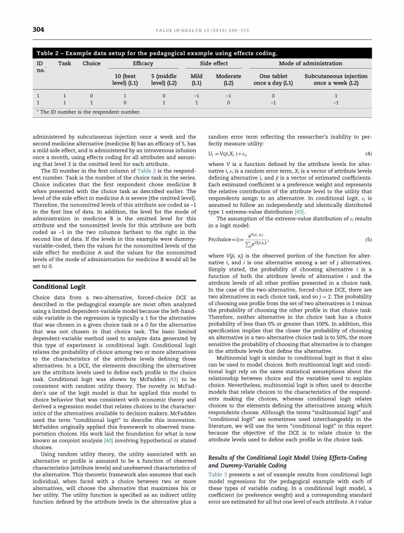
administered by subcutaneous injection once a week and thesecond medicine alternative (medicine B) has an efficacy of 5, hasa mild side effect, and is administered by an intravenous infusiononce a month, using effects coding for all attributes and assum-ing that level 3 is the omitted level for each attribute.

The ID number in the first column of Table 2 is the respond-ent number. Task is the number of the choice task in the series.Choice indicates that the first respondent chose medicine Bwhen presented with the choice task as described earlier. Thelevel of the side effect in medicine A is severe (the omitted level).Therefore, the nonomitted levels of this attribute are coded as –1in the first line of data. In addition, the level for the mode ofadministration in medicine B is the omitted level for thisattribute and the nonomitted levels for this attribute are bothcoded as –1 in the two columns farthest to the right in thesecond line of data. If the levels in this example were dummy-variable–coded, then the values for the nonomitted levels of theside effect for medicine A and the values for the nonomittedlevels of the mode of administration for medicine B would all beset to 0.

Conditional Logit

Choice data from a two-alternative, forced-choice DCE asdescribed in the pedagogical example are most often analyzedusing a limited dependent-variable model because the left-hand-side variable in the regression is typically a 1 for the alternativethat was chosen in a given choice task or a 0 for the alternativethat was not chosen in that choice task. The basic limiteddependent-variable method used to analyze data generated bythis type of experiment is conditional logit. Conditional logitrelates the probability of choice among two or more alternativesto the characteristics of the attribute levels defining thosealternatives. In a DCE, the elements describing the alternativesare the attribute levels used to define each profile in the choicetask. Conditional logit was shown by McFadden [43] to beconsistent with random utility theory. The novelty in McFad-den’s use of the logit model is that he applied this model tochoice behavior that was consistent with economic theory andderived a regression model that relates choices to the character-istics of the alternatives available to decision makers. McFaddenused the term “conditional logit” to describe this innovation.McFadden originally applied this framework to observed trans-portation choices. His work laid the foundation for what is nowknown as conjoint analysis [40] involving hypothetical or statedchoices.

Using random utility theory, the utility associated with analternative or profile is assumed to be a function of observedcharacteristics (attribute levels) and unobserved characteristics ofthe alternative. This theoretic framework also assumes that eachindividual, when faced with a choice between two or morealternatives, will choose the alternative that maximizes his orher utility. The utility function is specified as an indirect utilityfunction defined by the attribute levels in the alternative plus a

random error term reflecting the researcher’s inability to per-fectly measure utility:

Ui ¼Vðβ,Xi Þþεi, ð4Þwhere V is a function defined by the attribute levels for alter-native i, εi is a random error term, Xi is a vector of attribute levelsdefining alternative i, and β is a vector of estimated coefficients.Each estimated coefficient is a preference weight and representsthe relative contribution of the attribute level to the utility thatrespondents assign to an alternative. In conditional logit, εi isassumed to follow an independently and identically distributedtype 1 extreme-value distribution [43].

The assumption of the extreme-value distribution of εi resultsin a logit model:

Pr choice¼ ið Þ¼ eV β, xið ÞP

jeV β,xjð Þ , ð5Þ

where V(β, xi) is the observed portion of the function for alter-native i, and i is one alternative among a set of j alternatives.Simply stated, the probability of choosing alternative i is afunction of both the attribute levels of alternative i and theattribute levels of all other profiles presented in a choice task.In the case of the two-alternative, forced-choice DCE, there aretwo alternatives in each choice task, and so j ¼ 2. The probabilityof choosing one profile from the set of two alternatives is 1 minusthe probability of choosing the other profile in that choice task.Therefore, neither alternative in the choice task has a choiceprobability of less than 0% or greater than 100%. In addition, thisspecification implies that the closer the probability of choosingan alternative in a two-alternative choice task is to 50%, the moresensitive the probability of choosing that alternative is to changesin the attribute levels that define the alternative.

Multinomial logit is similar to conditional logit in that it alsocan be used to model choices. Both multinomial logit and condi-tional logit rely on the same statistical assumptions about therelationship between choice and the variables used to explainchoice. Nevertheless, multinomial logit is often used to describemodels that relate choices to the characteristics of the respond-ents making the choices, whereas conditional logit relateschoices to the elements defining the alternatives among whichrespondents choose. Although the terms “multinomial logit” and“conditional logit” are sometimes used interchangeably in theliterature, we will use the term “conditional logit” in this reportbecause the objective of the DCE is to relate choice to theattribute levels used to define each profile in the choice task.

Results of the Conditional Logit Model Using Effects-Codingand Dummy-Variable Coding

Table 3 presents a set of example results from conditional logitmodel regressions for the pedagogical example with each ofthese types of variable coding. In a conditional logit model, acoefficient (or preference weight) and a corresponding standarderror are estimated for all but one level of each attribute. A t value

Table 2 – Example data setup for the pedagogical example using effects coding.

IDno.*

Task Choice Efficacy Side effect Mode of administration

10 (bestlevel) (L1)

5 (middlelevel) (L2)

Mild(L1)

Moderate(L2)

One tabletonce a day (L1)

Subcutaneous injectiononce a week (L2)

1 1 0 1 0 –1 –1 0 11 1 1 0 1 1 0 –1 –1

* The ID number is the respondent number.

V A L U E I N H E A L T H 1 9 ( 2 0 1 6 ) 3 0 0 – 3 1 5304

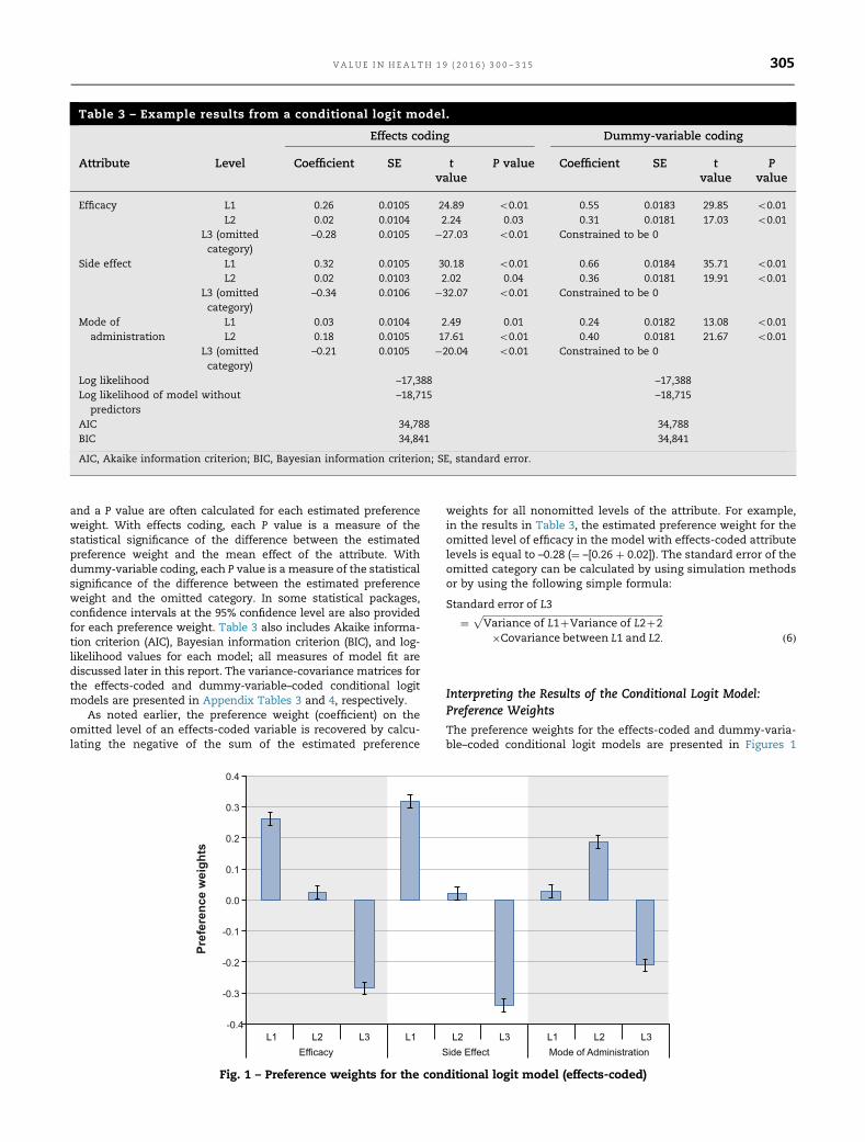
and a P value are often calculated for each estimated preferenceweight. With effects coding, each P value is a measure of thestatistical significance of the difference between the estimatedpreference weight and the mean effect of the attribute. Withdummy-variable coding, each P value is a measure of the statisticalsignificance of the difference between the estimated preferenceweight and the omitted category. In some statistical packages,confidence intervals at the 95% confidence level are also providedfor each preference weight. Table 3 also includes Akaike informa-tion criterion (AIC), Bayesian information criterion (BIC), and log-likelihood values for each model; all measures of model fit arediscussed later in this report. The variance-covariance matrices forthe effects-coded and dummy-variable–coded conditional logitmodels are presented in Appendix Tables 3 and 4, respectively.

As noted earlier, the preference weight (coefficient) on theomitted level of an effects-coded variable is recovered by calcu-lating the negative of the sum of the estimated preference

weights for all nonomitted levels of the attribute. For example,in the results in Table 3, the estimated preference weight for theomitted level of efficacy in the model with effects-coded attributelevels is equal to –0.28 (¼ –[0.26 þ 0.02]). The standard error of theomitted category can be calculated by using simulation methodsor by using the following simple formula:

Standard error of L3

¼ffiffiffiffiffiffiffiffiffiffiffiffiffiffiffiffiffiffiffiffiffiffiffiffiffiffiffiffiffiffiffiffiffiffiffiffiffiffiffiffiffiffiffiffiffiffiffiffiffiffiffiffiffiffiffiffiffiffiffiffiffiffiffiffiffiffiffiffiffiffiffiffiffiffiffiffiffiffiffiVariance of L1þVariance of L2þ2

p

�Covariance between L1 and L2: ð6Þ

Interpreting the Results of the Conditional Logit Model:Preference Weights

The preference weights for the effects-coded and dummy-varia-ble–coded conditional logit models are presented in Figures 1

Table 3 – Example results from a conditional logit model.

Effects coding Dummy-variable coding

Attribute Level Coefficient SE tvalue

P value Coefficient SE tvalue

Pvalue

Efficacy L1 0.26 0.0105 24.89 o0.01 0.55 0.0183 29.85 o0.01L2 0.02 0.0104 2.24 0.03 0.31 0.0181 17.03 o0.01

L3 (omittedcategory)

–0.28 0.0105 �27.03 o0.01 Constrained to be 0

Side effect L1 0.32 0.0105 30.18 o0.01 0.66 0.0184 35.71 o0.01L2 0.02 0.0103 2.02 0.04 0.36 0.0181 19.91 o0.01

L3 (omittedcategory)

–0.34 0.0106 �32.07 o0.01 Constrained to be 0

Mode ofadministration

L1 0.03 0.0104 2.49 0.01 0.24 0.0182 13.08 o0.01L2 0.18 0.0105 17.61 o0.01 0.40 0.0181 21.67 o0.01

L3 (omittedcategory)

–0.21 0.0105 �20.04 o0.01 Constrained to be 0

Log likelihood –17,388 –17,388Log likelihood of model without

predictors–18,715 –18,715

AIC 34,788 34,788BIC 34,841 34,841

AIC, Akaike information criterion; BIC, Bayesian information criterion; SE, standard error.

Fig. 1 – Preference weights for the conditional logit model (effects-coded)

V A L U E I N H E A L T H 1 9 ( 2 0 1 6 ) 3 0 0 – 3 1 5 305

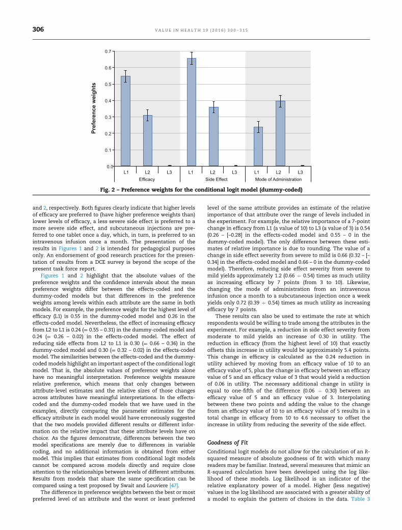
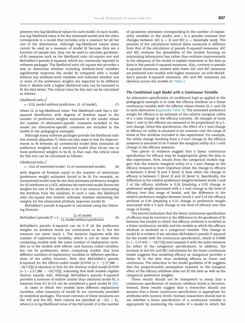
and 2, respectively. Both figures clearly indicate that higher levelsof efficacy are preferred to (have higher preference weights than)lower levels of efficacy, a less severe side effect is preferred to amore severe side effect, and subcutaneous injections are pre-ferred to one tablet once a day, which, in turn, is preferred to anintravenous infusion once a month. The presentation of theresults in Figures 1 and 2 is intended for pedagogical purposesonly. An endorsement of good research practices for the presen-tation of results from a DCE survey is beyond the scope of thepresent task force report.

Figures 1 and 2 highlight that the absolute values of thepreference weights and the confidence intervals about the meanpreference weights differ between the effects-coded and thedummy-coded models but that differences in the preferenceweights among levels within each attribute are the same in bothmodels. For example, the preference weight for the highest level ofefficacy (L1) is 0.55 in the dummy-coded model and 0.26 in theeffects-coded model. Nevertheless, the effect of increasing efficacyfrom L2 to L1 is 0.24 (¼ 0.55 – 0.31) in the dummy-coded model and0.24 (¼ 0.26 – 0.02) in the effects-coded model. The effect ofreducing side effects from L2 to L1 is 0.30 (¼ 0.66 – 0.36) in thedummy-coded model and 0.30 (¼ 0.32 – 0.02) in the effects-codedmodel. The similarities between the effects-coded and the dummy-codedmodels highlight an important aspect of the conditional logitmodel. That is, the absolute values of preference weights alonehave no meaningful interpretation. Preference weights measurerelative preference, which means that only changes betweenattribute-level estimates and the relative sizes of those changesacross attributes have meaningful interpretations. In the effects-coded and the dummy-coded models that we have used in theexamples, directly comparing the parameter estimates for theefficacy attribute in each model would have erroneously suggestedthat the two models provided different results or different infor-mation on the relative impact that these attribute levels have onchoice. As the figures demonstrate, differences between the twomodel specifications are merely due to differences in variablecoding, and no additional information is obtained from eithermodel. This implies that estimates from conditional logit modelscannot be compared across models directly and require closeattention to the relationships between levels of different attributes.Results from models that share the same specification can becompared using a test proposed by Swait and Louviere [47].

The difference in preference weights between the best or mostpreferred level of an attribute and the worst or least preferred

level of the same attribute provides an estimate of the relativeimportance of that attribute over the range of levels included inthe experiment. For example, the relative importance of a 7-pointchange in efficacy from L1 (a value of 10) to L3 (a value of 3) is 0.54(0.26 – [–0.28] in the effects-coded model and 0.55 – 0 in thedummy-coded model). The only difference between these esti-mates of relative importance is due to rounding. The value of achange in side effect severity from severe to mild is 0.66 (0.32 – [–0.34] in the effects-coded model and 0.66 – 0 in the dummy-codedmodel). Therefore, reducing side effect severity from severe tomild yields approximately 1.2 (0.66 C 0.54) times as much utilityas increasing efficacy by 7 points (from 3 to 10). Likewise,changing the mode of administration from an intravenousinfusion once a month to a subcutaneous injection once a weekyields only 0.72 (0.39 C 0.54) times as much utility as increasingefficacy by 7 points.

These results can also be used to estimate the rate at whichrespondents would be willing to trade among the attributes in theexperiment. For example, a reduction in side effect severity frommoderate to mild yields an increase of 0.30 in utility. Thereduction in efficacy (from the highest level of 10) that exactlyoffsets this increase in utility would be approximately 5.4 points.This change in efficacy is calculated as the 0.24 reduction inutility achieved by moving from an efficacy value of 10 to anefficacy value of 5, plus the change in efficacy between an efficacyvalue of 5 and an efficacy value of 3 that would yield a reductionof 0.06 in utility. The necessary additional change in utility isequal to one-fifth of the difference (0.06 C 0.30) between anefficacy value of 5 and an efficacy value of 3. Interpolatingbetween these two points and adding the value to the changefrom an efficacy value of 10 to an efficacy value of 5 results in atotal change in efficacy from 10 to 4.6 necessary to offset theincrease in utility from reducing the severity of the side effect.

Goodness of Fit

Conditional logit models do not allow for the calculation of an R-squared measure of absolute goodness of fit with which manyreaders may be familiar. Instead, several measures that mimic anR-squared calculation have been developed using the log like-lihood of these models. Log likelihood is an indicator of therelative explanatory power of a model. Higher (less negative)values in the log likelihood are associated with a greater ability ofa model to explain the pattern of choices in the data. Table 3

Fig. 2 – Preference weights for the conditional logit model (dummy-coded)

V A L U E I N H E A L T H 1 9 ( 2 0 1 6 ) 3 0 0 – 3 1 5306

presents two log-likelihood values for each model. In each model,one log-likelihood value is for the estimated model and the othercorresponds to a model that includes only a constant for all butone of the alternatives. Although log-likelihood values alonecannot be used as a measure of model fit because they are afunction of sample size, they can be used to calculate goodness-of-fit measures such as the likelihood ratio chi-square test andMcFadden’s pseudo R-squared, which are commonly reported insoftware packages. The likelihood ratio chi-square test provides away to determine whether including attribute-level variablessignificantly improves the model fit compared with a modelwithout any attribute-level variables and indicates whether oneor more of the preference weights are expected to be differentfrom 0. Models with a higher likelihood ratio can be assumed tofit the data better. The critical value for this test can be calculatedas follows:

Likelihood ratio χ2

¼�2 LL model without predictors�LL of model� �

, ð7Þwhere LL is log-likelihood value. The likelihood ratio has a chi-squared distribution with degrees of freedom equal to thenumber of preference weights estimated in the model minusthe number of alternative-specific constants included in themodel (no alternative-specific constants are included in themodel in the pedagogical example).

Although many software packages provide the likelihood ratiotest statistic (Equation 7), there are also ways to test for improve-ments in fit between an unrestricted model (that estimates allpreference weights) and a restricted model (that forces one ormore preference weights to be 0). In that case, the critical valuefor this test can be calculated as follows:

Likelihood ratio χ2

¼�2 LL of restricted model�LL of unrestricted modelð Þ, ð8Þwith degrees of freedom equal to the number of restrictions(preference weight estimates forced to be 0). For example, anunrestricted model may be one that estimates preference weightsfor all attributes in a DCE, whereas the restricted model forces theweights for one of the attributes to be 0 (in essence eliminatingthe attribute from the analysis). In such a case, the likelihoodratio chi-square test statistic indicates whether estimating theweights for the eliminated attribute improves model fit.

McFadden’s pseudo R-squared is calculated using the follow-ing formula:

McFadden's pseudo R2¼1� LL of modelLL model without predictors

: ð9Þ

McFadden’s pseudo R-squared can be 0 if all the preferenceweights on attribute levels are constrained to be 0, but themeasure can never reach 1. The measure improves with thenumber of explanatory variables, which is not an issue whencomparing models with the same number of explanatory varia-bles as in the models with effects- and dummy-coded variables,but can be problematic when comparing models that havedifferent numbers of explanatory variables or different specifica-tions of the utility function. Note that McFadden’s pseudoR-squared for the effects-coded model [0.0709 (¼ 1 – [–17,388 C–18,715])] is identical to that for the dummy-coded model [0.0709(¼ 1 – [–17,388 C –18,715])], indicating that both models explainchoices equally well. Although McFadden’s pseudo R-squaredprovides a measure of relative (rather than absolute) model fit, ameasure from 0.2 to 0.4 can be considered a good model fit [48].

In cases in which two models have different explanatoryvariables, other measures of model fit are commonly providedby statistical packages. The most common of these measures arethe AIC and the BIC. Both criteria are specified as �2LL þ Kγ,where LL is log-likelihood value of the full model, K is the number

of parameter estimates corresponding to the number of explan-atory variables in the model, and γ is a penalty constant thatchanges between AIC (γ ¼ 2) and BIC (γ ¼ ln[sample size]). Thepremise of the calculations behind these measures is differentfrom that of the calculation of pseudo R-squared measures. AICand BIC evaluate the plausibility of the models focusing onminimizing information loss rather than evaluate improvementsin the adequacy of the model to explain responses in the data asdone in the pseudo R-squared measures. Also, contrary to pseudoR-squared measures, models with lower AIC and BIC measuresare preferred over models with higher measures. As with McFad-den’s pseudo R-squared measures, AIC and BIC measures areidentical across the models in Table 3.

The Conditional Logit Model with a Continuous Variable

An alternative specification of conditional logit as applied to thepedagogical example is to code the efficacy attribute as a linearcontinuous variable with the efficacy values shown (3, 5, and 10)in each alternative (Appendix Table 5). The estimated preferenceweight for efficacy is an estimate of the relative marginal utilityof a 1-unit change in the efficacy outcome. All changes of morethan 1 unit in the efficacy are assumed to be proportional to a 1-unit change. Given this specification, the effect of a 1-unit changein efficacy on utility is assumed to be constant over the range oflevels of this attribute included in the experiment. For example,the utility change resulting from a 9-unit change in the efficacymeasure is assumed to be 9 times the marginal utility of a 1-unitchange in the efficacy measure.

Two pieces of evidence suggest that a linear continuousspecification for efficacy may be inappropriate given the data inthis experiment. First, results from the categorical models sug-gest that the relative marginal utility of a 1-unit change in theefficacy measure is more important when the change in efficacyis between 3 (level 3) and 5 (level 2) than when the change inefficacy is between 5 (level 2) and 10 (level 1). Specifically, thedifference in the relative preference weights between levels 1 and2 of the efficacy attribute is 0.24 (implying a 0.05 change inpreference weight associated with a 1-unit change in the level ofefficacy over this range of levels), and the difference in therelative preference weights between levels 2 and 3 of the efficacyattribute is 0.30 (implying a 0.15 change in preference weightassociated with a 1-unit change in the level of efficacy over thisrange of levels).

The second indication that the linear continuous specificationof efficacy may be incorrect is the difference in the goodness of fitbetween the models in which the efficacy attribute is modeled asa linear continuous variable and the models in which the efficacyattribute is modeled as a categorical variable. This change inmodel fit is evident if we calculate McFadden’s pseudo R-squaredfor the model with the continuous specification, which is 0.0686(¼ 1 – [–17,432 C –18,715]) and compare it with the same measurefor either of the categorical specifications. In addition, theincrease in the AIC and BIC calculations for the linear continuousmodel suggests that modeling efficacy as categorical provides abetter fit to the data than modeling efficacy as linear andcontinuous. The reduction in the model goodness of fit suggeststhat the proportionality assumption imposed on the marginaleffect of the efficacy attribute does not fit the data as well as thecategorical preference weights.

These results should not be interpreted to mean that acontinuous specification of numeric attribute levels is incorrect.Instead, these results suggest that a researcher should notassume that a linear continuous specification is appropriate forattributes with numeric levels. Instead, researchers should test tosee whether a linear specification of a continuous variable isappropriate by examining the results of a model in which the

V A L U E I N H E A L T H 1 9 ( 2 0 1 6 ) 3 0 0 – 3 1 5 307

numeric levels are treated as categorical. If a linear continuousspecification is not correct, the researcher can test for the appro-priateness of other nonlinear functional forms of this variable.

Limitations of Conditional Logit

There are two fundamental limitations of the conditional logitmodel. First, the model assumes that choice questions measureutility equally well (or equally poorly) across all respondents andchoice tasks (scale heterogeneity). Second, conditional logit doesnot account for unobserved systematic differences in preferencesacross respondents (preference heterogeneity). Although histor-ically these two problems have been considered distinct issues ofthe conditional logit model, more recent discussions acknowl-edge that the two problems are related [49].

The first problem is scale heterogeneity [50]. The conditionallogit model assumes that the ratio of estimated preferenceweights is exactly the same if both the numerator and thedenominator are multiplied by the same value [51]. Using condi-tional logit, this value is inversely related to a constant modelvariance normalized to 1 for all respondents. If, however, thevariance (i.e., the ability of the model to estimate utility) is notconstant across all respondents or across all choice tasks, differ-ences in model estimates between different respondents oracross different choice tasks may appear different when in factthey are not. For example, assume that the overall importance(difference between the highest and the lowest preferenceweights) of efficacy and the side effect are 0.80 and 0.20,respectively, for one group of choice tasks or one group ofrespondents in the sample and that the same values are 1.60and 0.40, respectively, for another group of choice tasks orrespondents. The absolute values of the relative importanceestimates for these two attributes are twice as large for thesecond group as they are for the first group; nevertheless, the ratioof the relative importance of efficacy to the side effect is the samein both groups. The scale in this case is constant. In some cases,however, assuming that the scale is constant across respondentsignores potential systematic variations in the model varianceacross choice questions or groups of individuals in the sampleand can result in biased estimates of preference weights [52].

The second potential problem with conditional logit is pref-erence heterogeneity—potential differences in relative preferen-ces across respondents in the sample. In effect, the conditionallogit model assumes that all respondents have the same prefer-ences that will yield a single set of preference weights. Theconditional logit model does not account for systematic varia-tions in preferences across respondents. Failing to account forheterogeneity in preferences can lead to biased estimates of thepreference weights.

The relationship between the two potential problems isclearer if we acknowledge that preference heterogeneity can becorrelated across attribute levels. That is, preferences for multipleattributes can increase or decrease together among specificindividuals in the sample. If variations in preferences are allowedto be correlated across respondents, preference heterogeneity canbehave exactly as scale heterogeneity does. That is, if a respond-ent’s preferences move proportionately together across attrib-utes, the ratios of preferences for any pair of attributes remainunchanged, whereas the absolute values of the preferenceweights would be different by a constant scaling factor, just asthey would with scale heterogeneity.

Alternatives to Conditional Logit

Several alternative statistical techniques have been proposed toovercome some, but not all, of the limitations of conditional logit.

Specifically, these models are able to address conditional logit’sinability to account for correlation among multiple responsesfrom each individual or heterogeneity in preferences across thesample. Alternative techniques continue to be developed; thisreport, however, focuses on three statistical methods that arecommonly used in health applications of DCEs. These statisticalmethods include RPL, HB, and LCM analyses. All three of thesemethods are based on limited dependent-variable models con-sistent with random utility theory and ensure that the predictedprobability of choosing any alternative is between 0% and 100%.Each of these techniques is more statistically complex thanconditional logit, but each has potential advantages. These threeapproaches are discussed in the following sections. Knowing thateffects-coded and dummy-coded models provide the same infor-mation, we will use the results from only the effects-codedmodels to characterize the alternatives to conditional logit inthe following sections of this report.

Random-Parameters Logit

Like conditional logit, RPL (also called “mixed-logit”) is a methodthat assumes that the probability of choosing a profile from a setof alternatives is a function of the attribute levels that character-ize the alternatives and a random error term that adjusts forindividual-specific variations in preferences. Unlike conditionallogit that estimates only a set of coefficients capturing the meanpreference weights of the attribute levels, RPL yields both a meaneffect and a standard deviation of effects across the sample. Thatis, RPL explicitly assumes that there is a distribution of prefer-ence weights across the sample reflecting differences in prefer-ences among respondents, and it models the parameters of thatdistribution for each attribute level. The choice probability of theRPL model is as follows:

Pr choicen¼ ið Þ¼ eV ~βn ,xið ÞP

jeV ~βn ,xjð Þ , ð10Þ

where n indexes respondents in the sample, ~βn ¼ f β,σjvnð Þ, β and σ

are parameters to be estimated on the basis of systematicvariations in preferences across individuals in the sample giventhe variable vn characterizing individual-specific heterogeneity,and f �ð Þ is a function determining the distribution of ~βn acrossrespondents, given parameters β and σ. Commonly, ~β is assumedto be normally distributed with mean β and standard deviation σ,which means the following:

~βn ¼f β,σjvnð Þ¼βþσvn, f or vn�N 0, 1ð Þ across respondents in the sample: ð11Þ

With this assumption about f ðnÞ, the choice probability of condi-tional logit is a special case of the RPL choice probability whereσ¼0. Larger (smaller) standard deviations indicate greater (lesser)variability in preference weights across respondents. Neverthe-less, little direct guidance is available to determine the appro-priate functional form for the distribution of preferences acrossrespondents. Because individual preference weights are notdirectly interpretable, it is often difficult to determine the dis-tributional characteristics of preferences in any given sample apriori.

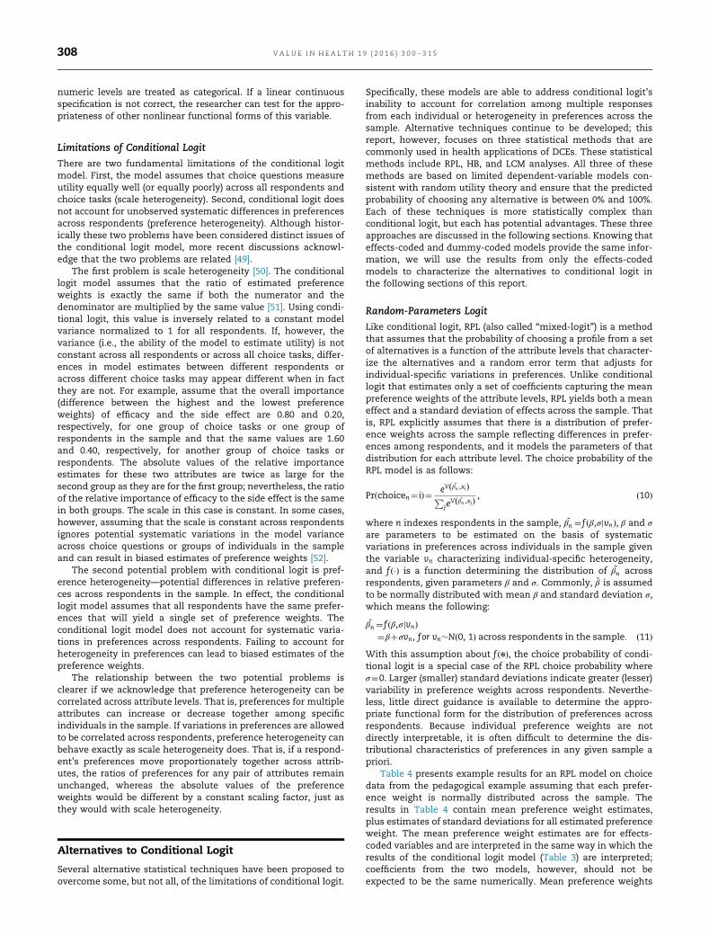
Table 4 presents example results for an RPL model on choicedata from the pedagogical example assuming that each prefer-ence weight is normally distributed across the sample. Theresults in Table 4 contain mean preference weight estimates,plus estimates of standard deviations for all estimated preferenceweight. The mean preference weight estimates are for effects-coded variables and are interpreted in the same way in which theresults of the conditional logit model (Table 3) are interpreted;coefficients from the two models, however, should not beexpected to be the same numerically. Mean preference weights

V A L U E I N H E A L T H 1 9 ( 2 0 1 6 ) 3 0 0 – 3 1 5308

from RPL are typically larger in magnitude than the preferenceweights from the same model estimated using conditional logit,but the relative relationships (e.g., ratios of changes in attributes)among preference weights for different attributes are typicallysimilar between the two sets of coefficients. Each standarddeviation indicates the distribution about the correspondingmean preference weight.

One issue with RPL models is that the maximum simulatedlikelihood estimation used to fit RPL models relies on a simu-lation technique that can produce different answers if theparameters of the simulations are not set to be the same acrossregressions. These parameters include the simulation randomseed, the number of draws, and the type of draws taken.Researchers should estimate the model with multiple startingpoints to ensure that the model converges to a stable solution.The estimator sometimes requires a lengthy estimation processthat is not guaranteed to converge under certain circumstancesand also requires specifying the number of simulations to beused in a regression; ensuring that these numbers are adequateadds burden to the researcher. The model is increasingly avail-able in various software packages, but not all model features areavailable in all packages.

Hierarchical Bayes

Conditional logit and RPL are used to estimate preferences over apopulation. Conditional logit yields estimates of mean preferenceweights for a sample. RPL yields estimates of both mean preferenceweights and the expected distribution of preference weights acrossthe sample. Although RPL results take into account individual-specific effects, it models these effects as deviations from the meanpopulation parameters. In contrast, HBmodels reverse the problemto generate preference estimates for each individual in the sampleand only supplement these individual-specific estimates withaggregate preference information to the degree that individual-specific preference information is insufficient.

Like RPL, the underlying choice-probability model in HB isconditional logit [53,54]. This choice-probability model, however,is used to model responses from each individual, and not allobservations in the sample. With HB, individual results are usedto construct the (joint posterior) distribution of preferenceweights across respondents, including the mean and standarddeviation for the preference weight for each attribute level. Aswith RPL, to calculate the mean and standard deviation ofpreferences for attribute levels, HB requires that the researcherassume the form of the distribution of each preference weight.

HB models evaluate choices in two levels:

1. The likelihood level, or lower level, in which individualchoices are modeled using conditional logit:

Pr choice¼ ið Þ¼ eV βn ,xið ÞP

jeV βn ,xjð Þ : ð12Þ

2. The sample level, or upper level, which is often assumed to bemultivariate-normal (or normal for each preference weight),although other distributions, including lognormal, triangular,and uniform, have been used. This level characterizes thevariation of preferences across respondents:

βn�N b,Wð Þ: ð13Þ

An algorithm (Gibbs sampler) estimates iteratively the lowerlevel and the upper level, individual-specific preference weightparameters (βn), the overall preference mean (b), and thevariance-covariance matrix of preferences across respondents(W). Essentially, b is calculated as the sample average of the βn,and W is calculated as the sample variance-covariance of the βn.Each βn tends toward a value that maximizes the likelihood themodel explains the pattern of responses to the series of choicetasks multiplied by the upper-level function characterizing the

Table 4 – Example results from a random-parameters logit model.

Attribute Level Coefficient SE t value P value

Mean estimatesEfficacy L1 0.32 0.0153 20.84 o0.01

L2 0.03 0.0124 2.32 0.02L3 (omitted category) –0.35 0.0162 –21.45 o0.01

Side effect L1 0.39 0.0162 23.84 o0.01L2 0.02 0.0137 1.67 0.10

L3 (omitted category) –0.41 0.0181 –22.54 o0.01Mode of administration L1 0.03 0.0116 2.52 0.01

L2 0.24 0.0187 12.56 o0.01L3 (omitted category) –0.26 0.0190 –13.94 o0.01

Standard deviation estimatesEfficacy L1 0.32 0.0160 20.05 o0.01

L2 0.16 0.0198 8.35 o0.01L3 (omitted category) 0.49 0.0254 19.16 o0.01

Side effect L1 0.35 0.0161 21.75 o0.01L2 0.25 0.0167 15.19 o0.01

L3 (omitted category) 0.60 0.0218 27.76 o0.01Mode of administration L1 0.10 0.0265 3.67 o0.01

L2 0.47 0.0169 27.88 o0.01L3 (omitted category) 0.57 0.0290 19.66 o0.01

Log likelihood of model –16,657Log likelihood of model without predictors –18,715AIC 33,337BIC 33,436

AIC, Akaike information criterion; BIC, Bayesian information criterion; SE, standard error.

V A L U E I N H E A L T H 1 9 ( 2 0 1 6 ) 3 0 0 – 3 1 5 309

distribution of preferences with mean b and variance-covarianceW. The multiplication of the likelihood value for the respondentby the function of the upper-level distribution essentially keepsestimates of individual-level preference weights consistent withthe assumed distribution of the sample preferences and notoverly far from the sample preference mean [55].

Table 5 presents results from HB estimated using data fromthe pedagogical example assuming effects-coded variables andnormally distributed variations in preferences across respond-ents. Table 5 also compares the HB estimates of means andstandard deviations of the estimated preference weights with thecorresponding results from the RPL model estimated using thesame assumptions. Although these results should not be com-pared numerically, Table 5 shows that both methods producesimilar results in this example.

HB estimation can be slower for certain specifications of thedistributions of preference weights (e.g., truncated distributionssuch as uniform and triangular distributions). HB estimation isimplemented in fewer software packages than is RPL. Under-standing the raw output of the HB estimation method requiressome knowledge of sampling methods and Bayesian statistics. Insome software packages, however, aggregate results are includedin addition to the individual-specific estimates. These aggregateresults could include sample-level means and standard deviations.

The means of the preference weight distributions in HB aresimilar to the mean preference weights estimated using condi-tional logit or RPL [56,57]. The standard deviation for eachpreference weight represents how different that preferenceweight is across respondents. Larger standard deviations meanthat respondents differ in their perception of that attribute level.If the objective of the research is to estimate preference weightsfor each individual in the sample, or when the sample size issmall, Bayesian procedures may provide a better approach toanalysis than the RPL model because the inference using the jointposterior distribution of preference weights can be conducted forany sample size [57]. Also, the HB procedure does not require theassumption of a common scale across respondents imposed inthe conditional logit and RPL models.

Latent-Class Finite-Mixture Model

The LCM assumes that attributes of the alternatives can haveheterogeneous effects on choices across a finite number ofgroups or classes of respondents. To account for this hetero-geneity, the model assumes that there are classes or segmentswithin a sample such that each class has preference weights thatare identical within the class and that are systematically differentfrom preference weights in other classes. Within each class, thepreference weights are estimated using conditional logit. The

number of classes is prespecified by the researcher. For example,if the analyst chooses to model the sample using three classes,three different sets of conditional logit coefficients are estimated,one for each class.

In the LCM, the choice probability is defined as follows:

Pr choice¼1ð Þ¼X

qPr choice¼ ijβq� �

πq, ð14Þ

where πq is a class-probability function indicating the probabilityof being in each of the different classes. The class-probabilityfunction is a specific multinomial logit function that can includeonly a constant term or can include explanatory variables relatingthe probability of class membership to respondent characteristics.The probabilities of class membership must sum to 1, so the class-probability functions of all but one class are identifiable. The class-probability function for the omitted class does not change freely.As a consequence, the explanatory variables in the class-probability function must be interpreted as those respondentcharacteristics that increase or decrease the probability of beingin one class relative to the probability of being in the omitted class.

The choice probability within a class q is estimated usingconditional logit:

Pr choice¼ ijβq� �

¼ eV βq ,xið ÞP

jeV βq ,xjð Þ : ð15Þ

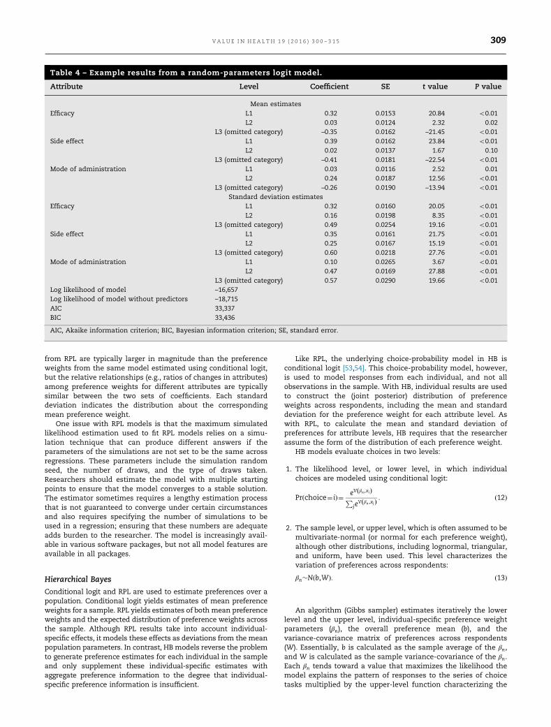
Table 6 presents example results for an LCM with two classesusing the effects-coded data from the pedagogical example. Itincludes a set of conditional logit model coefficients for each ofthe two classes and a class-probability function indicating theprobability that a respondent is in class 1. The class-probabilityfunction in this example includes only a constant and does notinclude any explanatory variables to test for the influence ofindividual characteristics on the probability of class membership.The class-probability estimate in this example indicates that, onaverage, a respondent in the sample has a 40% chance of being inclass 1. Because the class-probability function is estimated usingmultinomial logit and the log-odds coefficient for the constant inthe class-probability function is –0.40, the probability of being inclass 1 is calculated as follows:

40%¼ exp �0:40ð Þ1þexp �0:40ð Þ : ð16Þ

The results for each class in an LCM can be interpreted aspreference weights estimated with conditional logit. Neverthe-less, although the preference weights for the classes are esti-mated within a single model, parameters across classes aregenerally not directly comparable because they are confoundedwith a scale parameter that may differ between classes. There-fore, comparisons of preference weights across classes must be

Table 5 – Example results comparing RPL and HB models.

Attribute Level Mean Standard deviation estimates

RPL HB RPL HB

Efficacy L1 0.32 0.35 0.32 0.43L2 0.03 0.03 0.16 0.33L3 �0.35 �0.38 0.49 0.76

Side effect L1 0.39 0.43 0.35 0.50L2 0.02 0.03 0.25 0.42L3 �0.41 �0.46 0.60 0.92

Mode of administration L1 0.03 0.03 0.10 0.36L2 0.24 0.26 0.47 0.66L3 �0.26 �0.29 0.57 1.02

HB, hierarchical Bayes; RPL, random-parameters logit.

V A L U E I N H E A L T H 1 9 ( 2 0 1 6 ) 3 0 0 – 3 1 5310

done by evaluating the ratios of changes in preference weightsacross attributes. Sometimes, however, it is possible to evaluate theestimates across classes qualitatively to identify relevant differ-ences across classes. For example, the utility difference between L1and L2 in the mode of administration is positive (0.55) for class 1;for class 2, the same difference is negative (–0.63). Thus, one tabletonce a day is preferred to a subcutaneous injection once a week inclass 1, whereas the opposite is true for class 2.

In the LCM, there is no control for the effect of multipleobservations for each respondent. Usually it is assumed that,given the class assignment, multiple observations from the samerespondent are independent. Moreover, just as with conditionallogit and RPL, LCM does not control for potential scale hetero-geneity within each class; some software packages, however,include scale adjustments. As with RPL, researchers using LCMshould estimate the model with multiple starting points toensure that the model converges to a stable solution. Finally,determining the appropriate number of classes to include in amodel is challenging. AIC or BIC can be used to provide anobjective determination of the correct number of classes. Never-theless, using AIC may risk overfitting the model by having toomany classes and using BIC may risk underfitting the model byhaving too few classes [58]. Therefore, when determining theappropriate number of classes in an LCM, the researcher mustconsider the number of classes required to address the under-lying research questions and the ease of interpretation of multi-ple classes when the number of classes is large.

Discussion

This report describes a number of commonly used limiteddependent-variable analysis methods to analyze DCE data. Manyresearchers may be uncertain as to which method is the most

appropriate in any given circumstance, and, to a certain extent,there is no clear consensus on which methods are the best. Thefirst step in selecting a method is to understand the properties ofDCE data and the properties of the alternative methods availableto analyze it. Therefore, this report aimed to provide a descriptionof these methods and the advantages and limitations of each.The advantages and limitations are summarized in AppendixTable 6. We then provide a checklist of questions to considerwhen justifying the choice of analysis method, describing theanalysis, and interpreting the results (Table 7).

Conditional logit is the first limited dependent-variable anal-ysis method described in this report. Although conditional logithas a number of limitations, understanding conditional logit isfundamental to understanding the other analysis methodsdescribed in this report because these other analysis methodsare, in effect, extensions of conditional logit. Conditional logit canbe used to estimate average preferences across a sample but doesnot account for preference heterogeneity. Conditional logit isavailable in many software packages often used to analyze DCEdata. In addition, it is commonly used in LCMs or as a first step inRPL or HB analysis. Because conditional logit does not account forthe panel nature of the data, the results of a conditional logitanalysis could be biased. In addition, as a maximum-likelihoodmethod, conditional logit models may not converge, especiallyfor small samples or in the presence of substantial preferenceheterogeneity. The model, however, requires the smallest sam-ples for convergence among the options described in this report.

RPL is an analysis method that accounts for the panel natureof DCE data and allows preferences to vary across respondents inthe sample. It is becoming more commonly available in statisticalsoftware packages, but it is relatively more difficult to use andrequires the researcher to make assumptions about whichrandom parameters to include in the analysis and the distribu-tions of those random parameters. Because RPL estimates both

Table 6 – Example results of a latent-class model with two classes.

Attribute Level Coefficient SE t value P value

Class 1Efficacy L1 0.29 0.0246 11.70 o0.01

L2 0.04 0.0206 2.01 0.04L3 (omitted category) –0.33 0.0236 –13.98 o0.01

Side effect L1 0.39 0.0295 13.28 o0.01L2 –0.02 0.0235 –1.06 0.29

L3 (omitted category) –0.37 0.0248 –14.77 o0.01Mode of administration L1 0.21 0.0220 9.38 o0.01

L2 –0.33 0.0355 –9.25 o0.01L3 (omitted category) 0.12 0.0276 4.42 o0.01

Class 2Efficacy L1 0.27 0.0190 14.37 o0.01

L2 0.01 0.0164 0.80 0.42L3 (omitted category) –0.29 0.0187 –15.34 o0.01

Side effect L1 0.30 0.0214 14.20 o0.01L2 0.05 0.0177 3.09 o0.01

L3 (omitted category) –0.36 0.0192 –18.69 o0.01Mode of administration L1 –0.09 0.0172 –5.40 o0.01

L2 0.54 0.0277 19.60 o0.01L3 (omitted category) –0.45 0.0216 –20.84 o0.01

Class-probability functionConstant –0.40 0.0321 –12.46 o0.01

Log likelihood of model –16,985Log likelihood of model without predictors –18,715AIC 33,996BIC 34,103

AIC, Akaike information criterion; BIC, Bayesian information criterion; SE, standard error.

V A L U E I N H E A L T H 1 9 ( 2 0 1 6 ) 3 0 0 – 3 1 5 311

mean preference weights and distributions for preferenceweights, it may require larger sample sizes.

HB analysis provides a different way of modeling preferenceheterogeneity that can allow for the estimation of a choice modelfor each respondent. Under most circumstances, HB modelsconverge more quickly than models using alternative methods.Also, because HB models estimate preference weights for eachrespondent in the sample, they fully account for potential issuesof preference and scale heterogeneity (each respondent can havedifferent relative preferences, and the absolute values of thepreference weights can vary freely across respondents). Never-theless, because HB uses methods for updating preference esti-mates iteratively, it may be difficult to describe this method,which may lead to concerns that it is less transparent than otheranalysis methods. Also, because HB models do not estimate thesample-wide mean preference weights, but rather constructthem from the estimated individual preferences, practitionersneed to make inferences about overall effects using standarddeviations (variation of preferences across respondents) asopposed to using a standard error around a global estimate ofpreferences. At the same time, it is not possible to test for thesignificance of preferences for any given individual in the sample.

LCM provides a more parsimonious method for measuringpreference heterogeneity and modeling latent classes but oftenrequires specialized software or advanced macros in more

standard packages. It requires the researcher to specify thenumber of classes to be included in the model because objectivecriteria may result in too few or too many classes. This requiressignificant judgment on the part of the researcher, which may bedifficult to explain to users of the results. In addition, largersample sizes may be needed to accommodate the increase in thenumber of parameters to be estimated as the number of classesincreases.

Good Research Principles for Statistical Analysis

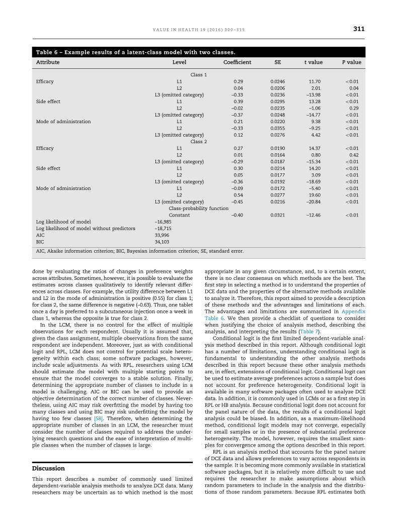
This report provides a description and an evaluation of manystatistical methods used to analyze DCE data on the basis of theconsensus of the task force that good research practices forthe statistical analysis of DCE data involve understanding thecharacteristics of alternative methods and ensuring thatthe interpretation of results is accurate. Taking into accountboth the assumptions made during the course of the analysisand the strengths and limitations of the analysis method toassist researchers in using the information presented in thisreport, the task force developed the ESTIMATE checklistcomposed of questions to consider when justifying thechoice of analysis method, describing the analysis, and inter-preting the results. Table 7 presents the ESTIMATE checklistquestions.

Table 7 – The ESTIMATE checklist.

ESTIMATE Recommendation

Estimates Describe the choice of parameter estimates resulting from the model appropriately and completely, including▪ Whether each variable corresponds to an effects-coded level, a dummy-coded level, or a continuous changein levels

▪ Whether each variable corresponds to a main effect or interaction effect▪ Whether continuous variables are linear or have an alternative functional form

Stochastic Describe the stochastic properties of the analysis, including▪ The statistical distributions of parameter estimates▪ The distribution of parameter estimates across the sample (preference heterogeneity)▪ The variance of the estimation function, including systematic differences in variance across observations (scaleheterogeneity)

Trade-offs Describe the trade-offs that can be inferred from the model, including▪ The magnitude and direction of the attribute-level coefficients▪ The relative importance of each attribute over the range of levels included in the experiment▪ The rate at which respondents are willing to trade off among the attributes (marginal rate of substitution)

Interpretation Provide interpretation of the results taking into account the properties of the statistical model, including▪ Conclusions that can be drawn directly from the results▪ Applicability of the sample, including subgroups or segments, to the population of interest▪ Limitations of the results

Method Describe the reasons for selecting the statistical analysis method used in the analysis, including▪ Why the method is appropriate for analyzing the data generated by the experiment▪ Why the method is appropriate for addressing the underlying research question▪ Why the method was selected over alternative methods

Assumptions Describe the assumptions of the model and the implications of the assumptions for interpreting the results,including

▪ Assumptions about the error distribution▪ Assumptions about the independence of observations▪ Assumptions about the functional form of the value function

Transparent Describe the study in a sufficiently transparent way to warrant replication, including descriptions of▪ The data setup, including handling missing data▪ The estimation function, including the value function and the statistical analysis method▪ The software used for estimation

Evaluation Provide an evaluation of the appropriateness of the statistical analysis method to answering the research question,including

▪ The goodness of fit of the model▪ Sensitivity analysis of the model specification▪ Consistency of results estimated using different methods

V A L U E I N H E A L T H 1 9 ( 2 0 1 6 ) 3 0 0 – 3 1 5312

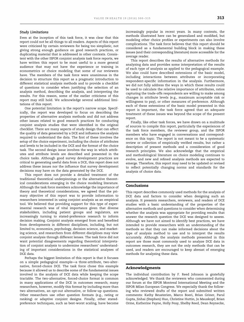
Study Limitations

Even at the inception of this task force, it was clear that thisreport could not be all things to all readers. Aspects of this reportwere criticized by certain reviewers for being too simplistic, notgiving strong enough guidance on good research practices, orduplicating material that is addressed in other contexts. Consis-tent with the other ISPOR conjoint analysis task force reports, wehave written this report to be most useful to a more generalaudience that may not have the experience or training ineconometrics or choice modeling that some of our reviewershave. The members of the task force were unanimous in thedecision to structure this report as a pragmatic introduction todifferent statistical analysis methods and to provide a checklistof questions to consider when justifying the selection of ananalysis method, describing the analysis, and interpreting theresults. For this reason, some of the earlier criticisms of thisreport may still hold. We acknowledge several additional limi-tations of this report.

One potential limitation is the report’s narrow scope. Specif-ically, the report was developed to focus on describing theproperties of alternative analysis methods and did not addressother issues related to good research practices for conductingconjoint analysis studies that were identified in the originalchecklist. There are many aspects of study design that can affectthe quality of data generated by a DCE and influence the analysisrequired to understand the data. The first of these involves thesetup of the choice experiment, including the choice of attributesand levels to be included in the DCE and the format of the choicetask. The second design issue involves the way in which attrib-utes and attribute levels are described and presented in thechoice tasks. Although good survey development practices arecritical to generating useful data from a DCE, this report does notaddress these issues nor the influence that survey developmentdecisions may have on the data generated by the DCE.

This report does not provide a detailed treatment of thetraditional theoretical underpinnings or the alternative theoret-ical considerations emerging in the choice modeling literature.Although the task force members acknowledge the importance oftheory and theoretical considerations, we agreed that the pri-mary objective of this report was to provide information toresearchers interested in using conjoint analysis as an empiricaltool. We believed that providing support for this type of exper-imental research was of vital importance given that diversestakeholders, including patient groups and regulators, areincreasingly turning to stated-preference research to informdecision making. Conjoint analysis emerged from and benefitedfrom developments in different disciplines, including, but notlimited to, economics, psychology, decision science, and market-ing science, and researchers from different disciplines may viewconjoint analysis through different lenses. The task force did notwant potential disagreements regarding theoretical interpreta-tion of conjoint analysis to undermine researchers’ understand-ing of important considerations in the statistical analyses ofDCE data.

Perhaps the biggest limitation of this report is that it focuseson a simple pedagogical example—a three-attribute, two-alter-native, forced-choice DCE. The task force chose this examplebecause it allowed us to describe some of the fundamental issuesinvolved in the analysis of DCE data while keeping the scopetractable. The two-alternative, forced-choice format is commonin many applications of the DCE in outcomes research; manyresearchers, however, modify this format by including more thantwo alternatives, an opt-out alternative, or follow-up questions.Other researchers use other question formats (e.g., rating orranking) or adaptive conjoint designs. Finally, other stated-preference techniques, such as best-worst scaling, have become

increasingly popular in recent years. In many contexts, themethods illustrated here can be generalized and modified, butmodeling other choice profiles or experiments can also involvecomplications. The task force believes that this report should beconsidered as a fundamental building block in making theseissues (and their corresponding literature) more accessible for theaverage reader.

This report describes the results of alternative methods foranalyzing data and provides some interpretation of the resultsof each type of analysis as applied to the pedagogical example.We also could have described extensions of the basic model,including interactions between attributes or incorporatingrespondent-specific information in the analysis. Furthermore,we did not fully address the ways in which these results couldbe used to calculate the relative importance of attributes, ratioscapturing the trade-offs respondents are willing to make amongchanges in attribute levels (e.g., maximum acceptable risk orwillingness to pay), or other measures of preference. Althougheach of these extensions of the basic model presented in thisreport is important, the task force agreed that an adequatetreatment of these issues was beyond the scope of the presentreport.

Finally, like other task forces, we have drawn on a multitudeof sources to compile this report, particularly the experiences ofthe task force members, the reviewer group, and the ISPORmembers who have engaged in conversations and correspond-ence on this topic. The report is not meant to be a systematicreview or collection of empirically verified results, but rather adescription of present methods and a consideration of goodresearch principles. We also acknowledge that the empiricaland methodological literature on choice modeling continues toevolve, and new and refined analysis methods are expected toemerge. Therefore, this report may need to be updated or revisedto reflect potentially changing norms and standards for theanalysis of choice data.

Conclusions

This report describes commonly used methods for the analysis ofDCE data and factors to consider when designing such ananalysis. It presents researchers, reviewers, and readers of DCEstudies with a basic understanding of the properties of thealternative methods and questions to consider when determiningwhether the analysis was appropriate for providing results thatanswer the research question the DCE was designed to assess.Although we have not aimed to identify best practices, we haveintended to provide researchers with an understanding of themethods so that they can make informed decisions about thetype of analysis method to use and to interpret the resultsaccurately. Although the analysis methods presented in thisreport are those most commonly used to analyze DCE data inoutcomes research, they are not the only methods that can beused, and readers are encouraged to keep abreast of emergingmethods for analyzing these data.

Acknowledgments

The individual contribution by F. Reed Johnson is gratefullyacknowledged. We thank the reviewers who commented duringour forum at the ISPOR Montreal International Meeting and theISPOR Milan European Congress. We especially thank the follow-ing who reviewed drafts of the report and submitted writtencomments: Kathy Beusterien, Marco Boeri, Brian Griner, ParulGupta, Jinhai (Stephen) Huo, Christine Huttin, Jo Mauskopf, BrianOrme, Katherine Payne, Holly Peay, Shelby Reed, Dean Reynecke,

V A L U E I N H E A L T H 1 9 ( 2 0 1 6 ) 3 0 0 – 3 1 5 313

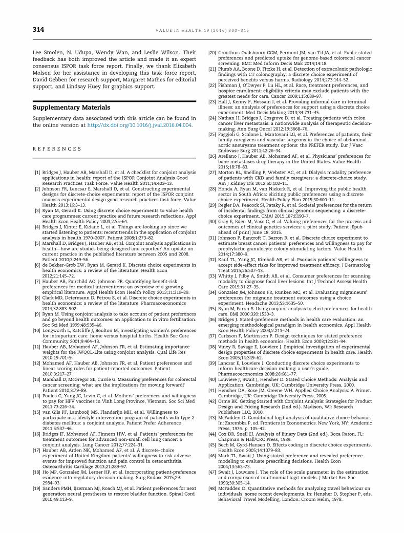
Lee Smolen, N. Udupa, Wendy Wan, and Leslie Wilson. Theirfeedback has both improved the article and made it an expertconsensus ISPOR task force report. Finally, we thank ElizabethMolsen for her assistance in developing this task force report,David Gebben for research support, Margaret Mathes for editorialsupport, and Lindsay Huey for graphics support.

Supplementary Materials

Supplementary data associated with this article can be found inthe online version at http://dx.doi.org/10.1016/j.jval.2016.04.004.

R E F E R E N C E S

[1] Bridges J, Hauber AB, Marshall D, et al. A checklist for conjoint analysisapplications in health: report of the ISPOR Conjoint Analysis GoodResearch Practices Task Force. Value Health 2011;14:403–13.

[2] Johnson FR, Lancsar E, Marshall D, et al. Constructing experimentaldesigns for discrete-choice experiments: report of the ISPOR conjointanalysis experimental design good research practices task force. ValueHealth 2013;16:3–13.

[3] Ryan M, Gerard K. Using discrete choice experiments to value healthcare programmes: current practice and future research reflections. ApplHealth Econ Health Policy 2003;2:55–64.

[4] Bridges J, Kinter E, Kidane L, et al. Things are looking up since westarted listening to patients: recent trends in the application of conjointanalysis in health 1970–2007. Patient 2008;1:273–82.

[5] Marshall D, Bridges J, Hauber AB, et al. Conjoint analysis applications inhealth—how are studies being designed and reported? An update oncurrent practice in the published literature between 2005 and 2008.Patient 2010;3:249–56.

[6] de Bekker-Grob EW, Ryan M, Gerard K. Discrete choice experiments inhealth economics: a review of the literature. Health Econ2012;21:145–72.

[7] Hauber AB, Fairchild AO, Johnson FR. Quantifying benefit-riskpreferences for medical interventions: an overview of a growingempirical literature. Appl Health Econ Health Policy 2013;11:319–29.

[8] Clark MD, Determann D, Petrou S, et al. Discrete choice experiments inhealth economics: a review of the literature. Pharmacoeconomics2014;32:883–902.

[9] Ryan M. Using conjoint analysis to take account of patient preferencesand go beyond health outcomes: an application to in vitro fertilisation.Soc Sci Med 1999;48:535–46.

[10] Longworth L, Ratcliffe J, Boulton M. Investigating women’s preferencesfor intrapartum care: home versus hospital births. Health Soc CareCommunity 2001;9:404–13.

[11] Hauber AB, Mohamed AF, Johnson FR, et al. Estimating importanceweights for the IWQOL-Lite using conjoint analysis. Qual Life Res2010;19:701–9.

[12] Mohamed AF, Hauber AB, Johnson FR, et al. Patient preferences andlinear scoring rules for patient-reported outcomes. Patient2010;3:217–27.

[13] Marshall D, McGregor SE, Currie G. Measuring preferences for colorectalcancer screening: what are the implications for moving forward?Patient 2010;3:79–89.

[14] Poulos C, Yang JC, Levin C, et al. Mothers’ preferences and willingnessto pay for HPV vaccines in Vinh Long Province, Vietnam. Soc Sci Med2011;73:226–34.

[15] van Gils PF, Lambooij MS, Flanderijn MH, et al. Willingness toparticipate in a lifestyle intervention program of patients with type 2diabetes mellitus: a conjoint analysis. Patient Prefer Adherence2011;5:537–46.

[16] Bridges JF, Mohamed AF, Finnern HW, et al. Patients’ preferences fortreatment outcomes for advanced non-small cell lung cancer: aconjoint analysis. Lung Cancer 2012;77:224–31.

[17] Hauber AB, Arden NK, Mohamed AF, et al. A discrete-choiceexperiment of United Kingdom patients’ willingness to risk adverseevents for improved function and pain control in osteoarthritis.Osteoarthritis Cartilage 2013;21:289–97.

[18] Ho MP, Gonzalez JM, Lerner HP, et al. Incorporating patient-preferenceevidence into regulatory decision making. Surg Endosc 2015;29:2984–93.

[19] Sanders PMH, IJzerman MJ, Roach MJ, et al. Patient preferences for nextgeneration neural prostheses to restore bladder function. Spinal Cord2010;49:113–9.

[20] Groothuis-Oudshoorn CGM, Fermont JM, van Til JA, et al. Public statedpreferences and predicted uptake for genome-based colorectal cancerscreening. BMC Med Inform Decis Mak 2014;14:18.

[21] Plumb AA, Boone D, Fitzke H, et al. Detection of extracolonic pathologicfindings with CT colonography: a discrete choice experiment ofperceived benefits versus harms. Radiology 2014;273:144–52.

[22] Fishman J, O’Dwyer P, Lu HL, et al. Race, treatment preferences, andhospice enrollment: eligibility criteria may exclude patients with thegreatest needs for care. Cancer 2009;115:689–97.

[23] Hall J, Kenny P, Hossain I, et al. Providing informal care in terminalillness: an analysis of preferences for support using a discrete choiceexperiment. Med Decis Making 2013;34:731–45.

[24] Nathan H, Bridges J, Cosgrove D, et al. Treating patients with coloncancer liver metastasis: a nationwide analysis of therapeutic decision-making. Ann Surg Oncol 2012;19:3668–76.

[25] Faggioli G, Scalone L, Mantovani LG, et al. Preferences of patients, theirfamily caregivers and vascular surgeons in the choice of abdominalaortic aneurysms treatment options: the PREFER study. Eur J VascEndovasc Surg 2011;42:26–34.

[26] Arellano J, Hauber AB, Mohamed AF, et al. Physicians’ preferences forbone metastases drug therapy in the United States. Value Health2015;18:78–83.

[27] Morton RL, Snelling P, Webster AC, et al. Dialysis modality preferenceof patients with CKD and family caregivers: a discrete-choice study.Am J Kidney Dis 2012;60:102–11.

[28] Honda A, Ryan M, van Niekerk R, et al. Improving the public healthsector in South Africa: eliciting public preferences using a discretechoice experiment. Health Policy Plan 2015;30:600–11.

[29] Regier DA, Peacock SJ, Pataky R, et al. Societal preferences for the returnof incidental findings from clinical genomic sequencing: a discrete-choice experiment. CMAJ 2015;187:E190–7.

[30] Gray E, Eden M, Vass C, et al. Valuing preferences for the process andoutcomes of clinical genetics services: a pilot study. Patient [Epubahead of print] June 18, 2015.

[31] Johnson P, Bancroft T, Barron R, et al. Discrete choice experiment toestimate breast cancer patients’ preferences and willingness to pay forprophylactic granulocyte colony-stimulating factors. Value Health2014;17:380–9.

[32] Kauf TL, Yang JC, Kimball AB, et al. Psoriasis patients’ willingness toaccept side-effect risks for improved treatment efficacy. J DermatologTreat 2015;26:507–13.

[33] Whitty J, Filby A, Smith AB, et al. Consumer preferences for scanningmodality to diagnose focal liver lesions. Int J Technol Assess HealthCare 2015;31:27–35.

[34] Gonzalez JM, Johnson FR, Runken MC, et al. Evaluating migraineurs’preferences for migraine treatment outcomes using a choiceexperiment. Headache 2013;53:1635–50.

[35] Ryan M, Farrar S. Using conjoint analysis to elicit preferences for healthcare. BMJ 2000;320:1530–3.

[36] Bridges J. Stated-preference methods in health care evaluation: anemerging methodological paradigm in health economics. Appl HealthEcon Health Policy 2003;2:213–24.

[37] Carlsson F, Martinsson P. Design techniques for stated preferencemethods in health economics. Health Econ 2003;12:281–94.

[38] Viney R, Savage E, Louviere J. Empirical investigation of experimentaldesign properties of discrete choice experiments in health care. HealthEcon 2005;14:349–62.

[39] Lancsar E, Louviere J. Conducting discrete choice experiments toinform healthcare decision making: a user’s guide.Pharmacoeconomics 2008;26:661–77.

[40] Louviere J, Swait J, Hensher D. Stated Choice Methods: Analysis andApplication. Cambridge, UK: Cambridge University Press, 2000.

[41] Hensher DA, Rose JM, Greene WH. Applied Choice Analysis: A Primer.Cambridge, UK: Cambridge University Press, 2005.

[42] Orme BK. Getting Started with Conjoint Analysis: Strategies for ProductDesign and Pricing Research (2nd ed.). Madison, WI: ResearchPublishers LLC, 2010.

[43] McFadden D. Conditional logit analysis of qualitative choice behavior.In: Zarembka P, ed. Frontiers in Econometrics. New York, NY: AcademicPress, 1974. p. 105–42.

[44] Cox DR, Snell EJ. Analysis of Binary Data (2nd ed.). Boca Raton, FL:Chapman & Hall/CRC Press, 1989.

[45] Bech M, Gyrd-Hansen D. Effects coding in discrete choice experiments.Health Econ 2005;14:1079–83.

[46] Mark TL, Swait J. Using stated preference and revealed preferencemodeling to evaluate prescribing decisions. Health Econ2004;13:563–73.

[47] Swait J, Louviere J. The role of the scale parameter in the estimationand comparison of multinomial logit models. J Market Res Soc1993;30:305–14.

[48] McFadden D. Quantitative methods for analyzing travel behaviour onindividuals: some recent developments. In: Hensher D, Stopher P, eds.Behavioral Travel Modelling. London: Croom Helm, 1978.

V A L U E I N H E A L T H 1 9 ( 2 0 1 6 ) 3 0 0 – 3 1 5314

[49] Hess S, Rose JM. Can scale and coefficient heterogeneity be separated inrandom coefficients models? Transportation 2012;39:1225–39.

[50] Greene WH, Hensher DA. Does scale heterogeneity across individualsmatter? A comparative assessment of logit models. Transportation2010;37:413–28.

[51] Ben-Akiva M, Lerman SR. Discrete Choice Analysis: Theory andApplication to Travel Demand. Cambridge, MA: MIT Press, 1985.

[52] Whitty JA, Ratcliffe J, Chen G, et al. Australian public preferences forthe funding of new health technologies: a comparison of discretechoice and profile case best-worst scaling methods. Med Decis Making2014;34:638–54.

[53] Allenby G, Rossi P. Marketing models of consumer heterogeneity.J Econom 1999;89:57–78.

[54] Allenby G, Lenk P. Modeling household purchase behavior with logisticnormal regression. J Am Stat Assoc 1994;89:1218–31.

[55] Train K. Discrete Choice Methods with Simulation. New York, NY:Cambridge University Press, 2003.

[56] Huber J, Train KE. On the similarity of classical and Bayesian estimatesof individual mean partworths. Mark Lett 2001;12:259–69.

[57] Regier DA, Ryan M, Phimister E, et al. Bayesian and classical estimationof mixed logit: an application to genetic testing. J Health Econ2009;28:598–610.

[58] Dziak JJ, Coffman DL, Lanza ST, Li R. Sensitivity and specificity ofinformation criteria. Methodology Center Technical Report #12-119.Penn State ScholarSphere. 2012. Available from: https://methodology.psu.edu/media/techreports/12-119.pdf. [Accessed March 19, 2016].

V A L U E I N H E A L T H 1 9 ( 2 0 1 6 ) 3 0 0 – 3 1 5 315