statistical methods - fb4all.com methods for... · statistical methods for practice and research a...
TRANSCRIPT


Statistical Methodsfor Practice and Research

2 STATISTICAL METHODS FOR PRACTICE AND RESEARCH

Statistical Methodsfor Practice and Research
�
A guide to data analysis using SPSS
(Second edition)
Ajai S. Gaur
Sanjaya S. Gaur
Copyright © Ajai S. Gaur and Sanjaya S. Gaur, 2009
All rights reserved. No part of this book may be reproduced or utilized in any form or by any means,electronic or mechanical, including photocopying, recording or by any information storage or retrievalsystem, without permission in writing from the publisher.
First published in 2006This Second Edition published in 2009 by
Response BooksBusiness books from SAGEB1/I-1 Mohan Cooperative Industrial AreaMathura Road, New Delhi 110 044, India
SAGE Publications Inc2455 Teller RoadThousand Oaks, California 91320, USA
SAGE Publications Ltd1 Oliver’s Yard, 55 City RoadLondon EC1Y 1SP, United Kingdom
SAGE Publications Asia-Pacific Pte Ltd33 Pekin Street#02-01 Far East SquareSingapore 048763
Published by Vivek Mehra for SAGE Publications India Pvt Ltd, typeset in 11/13.5 Palatino byStar Compugraphics Private Limited, Delhi and printed at Chaman Enterprises, New Delhi.
Library of Congress Cataloging-in-Publication Data Available
Gaur, Ajai S., 1977–Statistical methods for practice and research: a guide to data analysis
using SPSS/Ajai S. Gaur, Sanjaya S. Gaur.p. cm.
Includes bibliographical references.1. SPSS (Computer file) 2. Social sciences—Statistical methods—Computer programs. 3. Social
sciences—Research—Statistical methods.I. Gaur, Sanjaya S., 1969– II. Title.
HA32.G38 005.5'5—dc22 2006 2006015343
ISBN: 978-81-321-0100-0 (PB)
The SAGE Team: Reema Singhal, Madhula Banerji, Rajib Chatterjee and Trinankur Banerjee

To our parents
Shri Ram Saran and Smt. Sumitra

6 STATISTICAL METHODS FOR PRACTICE AND RESEARCH

Contents
Preface 11Acknowledgements 13
1. Introduction to SPSS 15
1.1 Starting SPSS 151.2 SPSS Main Menus 161.3 Working with the Data Editor 181.4 SPSS Viewer 221.5 Importing and Exporting Data 24
2. Basic Statistical Concepts 28
2.1 Research in Behavioral Sciences 282.1.1 Qualitative Research 282.1.2 Quantitative Research 29
2.2 Types of Variables 302.2.1 Qualitative Variables 302.2.2 Quantitative Variables 31
2.3 Reliability and Validity 312.3.1 Assessing Reliability 322.3.2 Assessing Validity 32
2.4 Hypothesis Testing 332.4.1 Type I and Type II Errors 352.4.2 Significance Level (p-value) 352.4.3 One-Tailed and Two-Tailed Tests 35
3. Summarizing Data: Descriptive Statistics 37
3.1 Basic Concepts 373.1.1 Measures of Central Tendency 383.1.2 Measures of Variability 383.1.3 Percentiles, Quartiles, and Interquartile Range 393.1.4 Skewness 39

8 STATISTICAL METHODS FOR PRACTICE AND RESEARCH
3.1.5 Kurtosis 403.2 Using SPSS 40
3.2.1 Descriptive Statistics 413.2.2 Frequencies 443.2.3 Tables 49
4. Comparing Means: One or Two Samples t-Tests 52
4.1 Basic Concepts 524.1.1 t-test and z-test 524.1.2 One Sample t-test 534.1.3 Independent Samples t-test 534.1.4 Dependent (Paired) Samples t-test 54
4.2 Using SPSS 544.2.1 One Sample t-test 544.2.2 Independent Samples t-test 584.2.3 Dependent Samples t-test 63
5. Comparing Means: Analysis of Variance 67
5.1 Basic Concepts 675.1.1 ANOVA Procedure 675.1.2 Factors and Covariates 685.1.3 Between, Within, and Mixed (Between-Within) Designs 695.1.4 Main Effects and Interactions 695.1.5 Post-Hoc Multiple Comparisons 705.1.6 Contrast Analysis 70
5.2 Using SPSS 705.2.1 One-Way Between-Groups ANOVA 715.2.2 Unplanned and Planned Comparisons 785.2.3 Two-Way Between-Groups ANOVA 85
6. Chi-Square Test of Independence for Discrete Data 91
6.1 Basic Concepts 916.1.1 Chi-Square Test of Independence 926.1.2 Contingency Tables 93
6.2 Using SPSS 93

CONTENTS 9
7. Correlation Analysis 99
7.1 Basic Concepts 997.1.1 Correlation Coefficient 997.1.2 Nature of Variables 1007.1.3 Bivariate/Partial Correlation 100
7.2 Using SPSS 1017.2.1 Bivariate Correlation 1037.2.2 Partial Correlation 105
8. Multiple Regression 108
8.1 Basic Concepts 1088.1.1 Regression Coefficient 1088.1.2 R Values 1098.1.3 Design Issues 1098.1.4 Multiple Regression Types 110
8.2 Using SPSS 1108.2.1 Standard Multiple Regression 1118.2.2 Hierarchical Regression 117
9. Logistic Regression 121
9.1 Basic Concepts 1219.1.1 Logistic Regression Coefficients 1219.1.2 Fit Indices 1229.1.3 Design Issues 1229.1.4 Logistic Regression Types 122
9.2 Using SPSS 123
10. Data Reduction and Scale Reliability: Factor Analysis 131
10.1 Basic Concepts 13110.1.1 Factor and Component 13110.1.2 Exploratory and Confirmatory Factor Analysis 13210.1.3 Extraction 13210.1.4 Factor Loadings 13210.1.5 Rotation 13310.1.6 Communalities 133

10 STATISTICAL METHODS FOR PRACTICE AND RESEARCH
10.1.7 Eigenvalue and Scree Plot 13310.1.8 Scale Reliability 13410.1.9 Sample Size Considerations 134
10.2 Using SPSS 13410.2.1 Factor Analysis 13410.2.2 Scale Reliability 145
11. Advanced Data Handling in SPSS 152
11.1 Sorting Cases 15211.2 Merging Files 15411.3 Aggregating Cases 15711.4 Splitting Files 16011.5 Selecting Cases 16211.6 Recoding Values 16411.7 Computing New Variables 168
Bibliography 170About the Authors 171

Preface
For business managers and practicing researchers, many times it becomesdifficult to solve the real life problems involving statistical methods usingsoftware packages. The books on managerial statistics do give a compre-hensive picture of statistics as a facilitating tool for managerial decisionmaking but they invariably fail in helping the manager/researcher insolving and getting results for practical problems. With the help of simpleexamples, these books very successfully explain simple calculation pro-cedures as well as the concepts behind them. However manual calculations,being cumbersome, tiresome and error-prone can be successful only to theextent of explaining the concepts and not for solving the real life researchproblems involving huge amount of data.
For this reason, most of the practical statistical analyses is done with thehelp of an appropriate software package. A manager/researcher, is onlyrequired to prepare the input data and should be able to get the final resulteasily with the help of software packages, so that focused attention can begiven to various other aspects of problem solving and decision making.
A wide variety of software packages such as SPSS, Minitab, SAS, STATA,S-PLUS etc. are available for statistical analyses. Microsoft Excel can alsobe used very successfully to solve a wide variety of problems. Some bookson managerial statistics even provide with spreadsheet templates wheredifferent results can be obtained by changing the input data. However,without the practical knowledge of working with a specialized softwarepackage, such templates are not helpful beyond academic interest.
This book is an effort towards facilitating business managers and re-searchers in solving statistical problems using computers. We have chosenSPSS, which is a very comprehensive and widely available package forstatistical analyses. We have illustrated its use with the help of simplepractical problems. The objective is to make the readers understand howthey can use various statistical techniques for their own research problems.Throughout the book, the point and click method has been used in place ofwriting the syntax, even though syntax has been provided for interestedusers at the end of each analysis. The advantage of the point and clickmethod is that it does not require any advance knowledge of the syntax

12 STATISTICAL METHODS FOR PRACTICE AND RESEARCH
and altogether eliminates the need to learn different types of command fordifferent analyses.
The book is aimed primarily at academic researchers, MBA students,doctoral, masters and undergraduate students of mathematics, managementscience, and various other science and social science disciplines, practicingmanagers, marketing research professionals etc. It is also expected to serveas a companion volume to any standard textbook of Statistics and MarketingResearch and for use in such courses in business schools and engineeringcolleges.
The book comprises of 11 chapters. Chapter 1 presents a brief overviewof SPSS. Chapter 2 gives an overview of basic statistical concepts with theaim of helping in a quick revision of basic concepts, which one commonlyencounters while carrying out data analyses. For an in-depth understandingof these concepts, readers are advised to refer to any standard textbook onstatistics. Chapter 3 presents the use of SPSS in calculating descriptive stat-istics and presenting a visual display of the data. Chapters 4 and 5 presentstatistical techniques for comparing means of two or more than two groups.Chapter 6 describes a chi-square test for discrete data. Correlation analysesis presented in Chapter 7, followed by multiple regression in Chapter 8 andlogistic regression in Chapter 9. Finally, we present data reduction techniquesand methods for establishing scale reliability in Chapter 10 and advanceddata handling and manipulation techniques in Chapter 11.
The illustrations are based on the SPSS 16.0 version. However, earlierversions of SPSS (10, 11, 12, 13, 14, 15) are functionally not much differentfrom this version. The users of the earlier versions will find it equally usefulfor their purpose. With this book, we hope, you can analyze your data onyour own and appreciate the real use of statistics.

Acknowledgements
Many people have made this book possible. We would especially like tothank our students and participants of the research methods workshopswe conducted all over India for refining our thinking and for motivating usto write a text on this subject. Our sincere thanks are due to Andrew Deliosfor his unusual tutelage on finer aspects of data analyses. The publishingteam at SAGE, New Delhi has been very helpful. Leela, Shweta, and Aninditaneed special mention for their patience and support during the publicationprocess. We would also like to thank Chapal, without whose persistencethis book would have never come out. Finally, we thank our families—Sanjaya’s family: Nirmal, Kamakhsi, and Vikrant and Ajai’s family: Deekshaand Dishita—for their continued support and encouragement, withoutwhich this project would not have been attempted, much less finished.
Ajai S. GaurSanjaya S. Gaur

14 STATISTICAL METHODS FOR PRACTICE AND RESEARCH

1
Introduction to SPSS
SPSS is a very powerful and user friendly program for statistical analyses.Anyone with a basic knowledge of statistics who is familiar with MicrosoftOffice can easily learn how to run very complicated analyses in SPSS witha simple click of the mouse. We begin this chapter from how to open theSPSS program and go on to explain different menus on the tool bar, thestarting commands, and the basic procedures of data entry.
1.1 STARTING SPSS
The SPSS program can be installed in a computer using a CD or from thenetwork. Once installed, SPSS can be opened like any other Windows-basedapplication by clicking on the Start menu at the bottom left hand corner ofthe screen and clicking on SPSS for Windows from the list of programs.Opening the SPSS program for the first time will produce a dialog box asshown in Figure 1.1. This dialog box is not of any particular use, selectDon’t show this dialog in the future, and click on the Cancel button. Thisactivates a window as shown in Figure 1.2. This is the main data editorwindow where all the data is entered, much like an Excel spreadsheet. Aquick look at this screen (Figure 1.2) reveals that it is quite similar to mostof the other Windows-based applications such as MS Excel.
At the top of the screen there are different menus, which give access tovarious functions of SPSS. Below this, there is a toolbar, which has buttonsfor quick access to various functions. The same functions can be performedby choosing relevant options from the menus. At the bottom of the screenwe have a status bar. At the bottom of Figure 1.2, we can see SPSS Processoris ready in the status bar. It implies that SPSS has been installed properly

16 STATISTICAL METHODS FOR PRACTICE AND RESEARCH
and the license is valid. If the analysis is being run by the processor, statusbar shows a message to that effect. The program can be closed by clickingon the Close button at the top right hand corner, just like in any otherWindows application software.
1.2 SPSS MAIN MENUS
SPSS 16.0 has 11 main menus, which provide access to every tool of theSPSS program. You can see the menus on the top of Figure 1.2. Readersmust be familiar with some of the menu items like File, Edit etc. as these are
Figure 1.1

INTRODUCTION TO SPSS 17
commonly encountered while working on Microsoft Office applications. Wewill go through the menus in this section.
The File, Edit, and View menus are very similar to what we get on openinga spreadsheet. The File menu lets us open, save, print, and close files andprovides access to recently used files. The Edit menu lets us do things likecut, copy, paste etc. The View menu lets us customize the SPSS desktop. Usingthe View menu we can hide or show the toolbar, status bar, gridlines etc.
The Data menu is an important tool in SPSS. It allows us to manipulatethe data in various ways. We can define variables, go to a particular case,sort cases, transpose them, merge cases as well as variables from some otherfile. We can also select cases on which we want to run the analysis andsplit the file to arrange the output of the analysis in a particular manner.The Transform menu is another very useful tool, which lets us compute newvariables and make changes to existing ones.
Figure 1.2

18 STATISTICAL METHODS FOR PRACTICE AND RESEARCH
The Analyze menu is the function which lets us perform all the statisticalanalyses. This has various statistical tools categorized under different cat-egories. The Graphs menu lets us make various types of plots from our data.The Utilities menu gives us information about variables and files. TheAdd-ons tells us about other programs of the SPSS family such as Amos,Clementine etc. In addition, we can find the newly added functions underAdd-ons. Finally, the Window and Help menus are very similar to otherWindows application menus.
1.3 WORKING WITH THE DATA EDITOR
The screen in Figure 1.2 is the data editor. In SPSS 13.0 and earlier versions,one could open only one data editor window at a time, however in SPSS14.0 and later versions, multiple data editor windows can be opened simul-taneously, much like Microsoft Excel. At the bottom of the data editor thereare two tabs—Data View and Variable View. In Data View, the data editorworks pretty much in the same manner as an Excel spreadsheet. One canenter values in different cells, modify them and even cut and paste to andfrom an Excel spreadsheet. In Variable View, the data editor window looksas shown in Figure 1.3. In addition to entering the values of the variables,we have to provide information about them in SPSS. This can be done whenthe data editor is in Variable View. Notice that there are 10 columns in thedata editor window in Figure 1.3. We will explain the usage of each of themwith the help of following small exercise of data entry:
Suppose we want to enter the following data in SPSS:
Respondent Gender Age(M=1, F=2)
1 1 252 1 223 2 204 2 275 2 28

INTRODUCTION TO SPSS 19
We have three variables to enter—respondent number, gender, and age.The first column in the variable view is Name. Earlier versions of SPSS (SPSS12.0 and earlier) could take a maximum of eight characters starting with aletter to identify a variable. There is no limit for the length of variable namein the later versions. In this example, we will name respondent number asresp_id; gender and age can be named as they are. The next column titledType lets us define the variable type. If we click on the cell next to variable nameand in the Type column, we get a dialog box as shown in Figure 1.4.
Figure 1.4
Figure 1.3

20 STATISTICAL METHODS FOR PRACTICE AND RESEARCH
Data can be of several types, including numeric, date, text etc. An incorrecttype-definition may not always cause problems, but sometimes does, andshould therefore be avoided. The most common type used is “Numeric,”which means that the variable has a numeric value. The other commonchoice is “String,” which means that the variable is in text format. We cannotperform any statistical analysis on a numeric variable if it is specified as astring variable. Below is a table showing the data types:
Type Example
Numeric 1,000.01
Comma 1,000.01
String IIT Bombay
Since all our three variables are of the numeric type, we select numericfrom the dialog box shown in Figure 1.4. We can also specify the width ofthe variable column and decimal places on this dialog box. It only affectsthe way variables are shown when the data editor is on data view. Click onOK to return to the data editor. Next two columns titled Width and Decimalsalso allow us to specify these factors for the data view. Please note thatthese have no impact on the actual values we enter in the data editor, theyonly affect the display of the data. For example if the value of a variable ina particular cell is 100000000, which comprises of 9 digits and we have spe-cified the width for this variable as 8, it will appear as ########. This simplymeans that the width of the variable column is not enough to display thevariable correctly.
Next, we have a column titled Label. Since the variable name in the firstcolumn can only be of 8 characters in the earlier versions of the SPSS pro-gram, it is sometimes difficult to identify the variable by its name. To avoidthis problem, we can write the details about a particular variable in thiscolumn. For example, we can write “Respondent identification number” asthe label for resp_id variable. We can ask the SPSS program to show variablelabels with or without the names in the output window. This option can beactivated by selecting “Names” and “Labels” from the dialog box obtainedby clicking Edit → Options → Output Labels.
Then, we have a column labeled Values. If we click on the cell next to thevariable name and in the Values column, we get a dialog box as shown inFigure 1.5. In this box, we can specify values for our variables. In the example

INTRODUCTION TO SPSS 21
here, we have two values for gender—1 representing male and 2 repre-senting female. Enter 1 in the empty box labeled Value and specify its name(Male) in the next box labeled Value Label. This will activate the Add button.Click on this button and repeat these steps to specify female. This way wecan keep track of the actual status of qualitative variables such as gender,nation, race, color etc.
After Values we have a column labeled Missing to specify missing values.While coding data, we often specify certain numbers to variables for whichsome respondents have given no response. Unless we specify these valuesas missing values, SPSS will take them into consideration for data analysesproducing a wrong output. One way to handle this problem is to recodethese numbers to missing values. The Recode command has been discussedin Section 11.6. The other way is to specify the number that should be con-sidered as missing values here itself. Clicking on the cell next to the variablename and in the Missing column will produce a dialog box as shown inFigure 1.6. By default, No missing values is selected here. We can specify upto three discrete values to be considered as missing values. Alternatively,specify a range and all the values in the range will be considered as missingvalues. In case there are more than three discrete values that cannot bespecified as a range, use the Recode command from the Transform menu(see Figure 1.2).
The next two columns titled Columns and Align help us modify the waywe want to view the data on screen. In the Columns column we can specify
Figure 1.5

22 STATISTICAL METHODS FOR PRACTICE AND RESEARCH
the width of the column and in the Align column we can specify if we wantour data to be right, left or center aligned. These do not have any impact onthe actual data analyses. Finally, in the column titled Measure, we can specifywhether our variable is scale, ordinal, or nominal. SPSS treats interval andratio data as scale. Different categories of variables are explained in Chapter 2.
Once the variables are specified, you can switch to Data View and enter thedata. The data editor on entering the data will look as shown in Figure 1.7.This data file can be saved just as an MS Word or MS Excel file and reopenedby double clicking on the file from its saved location.
1.4 SPSS VIEWER
Whenever we run any command in SPSS, the output is shown in the SPSSViewer which opens as a separate window. We can also specify the com-mands to be displayed in a log in the Viewer window. This option can beactivated by selecting Display commands in log option on the dialog box,obtained by clicking Edit → Options → Viewer. If this option is selected, aViewer window will open displaying the save command once we save thefile. The Viewer window is shown in Figure 1.8.
The SPSS Viewer window has two panels. The right hand panel showsthe actual output and log of commands (if the same is activated), the lefthand panel shows an outline of the output shown in the right hand panel.One can quickly navigate through the output by selecting the same fromthe outline provided in the left hand panel.
Figure 1.6

INTRODUCTION TO SPSS 23
The menu items are quite similar to what we find on the Data Editor.However, here we have two additional menus—Insert and Format. The Insertcommand can be used to insert headings, comments, page breaks etc. toorganize the output if the output file is very large. The Format command hasa similar role of arranging the output in a user friendly manner. The Formatcommand is rarely used as the output can be copied and pasted onto a MSWord or MS Excel file. The output can also be exported to a variety of otherformats. The export option can be accessed under the File menu. Clicking
Figure 1.7
Figure 1.8

24 STATISTICAL METHODS FOR PRACTICE AND RESEARCH
on Export will produce a dialog box as shown in Figure 1.9. On this windowwe can specify the part of the output we want to export by making anappropriate selection in the box titled Objects to Export. We can also specifythe format of the exported file by selecting a particular type from the dropdown menu below Type. SPSS provides several formats in which the outputcan be exported—HTML file, Text file, Excel file, PDF file, Presentation file,and Word/RTF file.
Figure 1.9
1.5 IMPORTING AND EXPORTING DATA
SPSS gives users a variety of options to open a data file. Click on File →Open → Data as shown in Figure 1.10. This will produce a dialog box(Figure 1.11).
Here we can choose the types of file we want to open in SPSS. The filetype can be chosen from the drop down menu against Files of Type as shown

INTRODUCTION TO SPSS 25
Figure 1.10
in Figure 1.11. SPSS 16.0 can open data files from programs like Excel, Systat,Lotus, dBase, SAS, STATA in addition to text and ASCII formats. SPSS 14.0and later versions are an improvement as these can support more file typessuch as STATA files, which was not possible in earlier versions.
If we want to open data from an Excel file, we select the file and clickon Open. This will produce a dialog box as shown in Figure 1.12. In thisbox, we can specify the specific work sheet from which we want to importthe data. We can also read the variable names if the same have been specifiedin the Excel sheet by clicking on a small box against Read variable names fromthe first row of data. Please note that if the variable names specified in Excelhave more than eight characters, SPSS 12.0 and earlier versions would assign

26 STATISTICAL METHODS FOR PRACTICE AND RESEARCH
Figure 1.11
Figure 1.12

INTRODUCTION TO SPSS 27
a name to them automatically as they do not support variable names biggerthan eight characters.
Just as we can import data into SPSS from many formats, we can alsosave an SPSS data file into different formats. This can be done by click-ing on File Save as and selecting the required format in the resulting dialogbox.

2
Basic Statistical Concepts
Computers have changed the way statistics is learned and taught. Often,students of behavioral sciences are interested only in the “results” of their“analyses” and do not care about how the results are obtained. The purposeof this chapter is to introduce such readers to the common statistical termsand concepts which one must know in order to interpret computer generatedoutputs. This is not to under-emphasize the value of learning the nitty-gritty of statistical techniques. Readers are strongly recommended to referto some standard statistical textbook in order to understand the underlyingtheory and logic. However, as the objective of this book is to help studentsuse SPSS for their research, we limit the discussion in this chapter to thepractical aspects of statistics necessary for using a software package, capableof doing statistical analyses for us.
2.1 RESEARCH IN BEHAVIORAL SCIENCES
One of the main objectives of a behavioral scientist is to develop theories andprinciples which provide insights into human and organizational behavior.These theories and principles have to be evaluated against actual observa-tions. This is called the validation of theories by empirical research. Broadly,research can be classified into two groups—qualitative research andquantitative research.
2.1.1 Qualitative Research
Qualitative research involves collecting qualitative data by way of in-depthinterviews, observations, field notes, open-ended questions etc. The researcher
BASIC STATISTICAL CONCEPTS 29
himself is the primary data collection instrument, and the data could becollected in the form of words, images, patterns etc. Data analysis involvessearching for patterns, themes, and holistic features. Results of such researchare likely to be context specific and reporting takes the form of a narrativewith contextual description and direct quotations from researchers.
2.1.2 Quantitative Research
Quantitative research involves collecting quantitative data based on precisemeasurement using structured, reliable, and validated data collection instru-ments or through archival data sources. The nature of the data is in theform of variables and data analysis involves establishing statistical rela-tionships. If properly done, results of such research are generalizable toentire populations. Without any specific prejudice against these two researchapproaches, the rest of the book deals only with quantitative research.
Quantitative research could be classified into two groups dependingon the data collection methodologies—experimental research and non-experimental research. The choice of statistical analysis depends on thenature of the research.
Experimental Research forms the basis of much of the psychologicalresearch. The main purpose of experimental research is to establish a causeand effect relationship. Please note that it is only in a properly designedexperimental research that a researcher can establish a cause and effectrelationship conclusively. The defining characteristics of experimentalresearch are active manipulation of independent variables and the randomassignment of participants to the conditions which represent these vari-ations. Other than the independent variables to be manipulated, everythingelse should be kept as similar and as constant as possible.
To depict the way experiments are conducted, we use the term “design ofexperiment”. There are two main types of experimental designs—between-subjects design and within-subjects design. In a between-subjects design,we randomly assign different participants to different conditions. On theother hand, in a within-subjects design the same participants are randomlyallocated to more than one condition. It is also referred to as repeated measuresdesign. In addition to having a purely between-subjects or within-subjectsdesign, one can also have a mixed design experiment. The commonly usedtechniques for analyzing such data include t-tests, ANOVA etc.

30 STATISTICAL METHODS FOR PRACTICE AND RESEARCH
Non-Experimental Research is commonly used in sociology, political sci-ence, and management disciplines. This kind of research is often done withthe help of a survey. There is no random assignment of participants to a par-ticular group, nor do we manipulate the independent variables. As a result,one cannot establish a cause and effect relationship through non-experimentalresearch. There are two approaches to analyzing such data. First is testingfor significant differences across the groups (such as IQ levels of participantsfrom different ethnic backgrounds), while the second is testing for signifi-cant association between two factors (such as firm sales and advertisingexpenditure).
Quantitative research is also classified based on the type of data used asprimary and secondary data research. Primary data is the one which wecollect directly from the subjects of study. This is done with the help ofstandard survey instrument. An example of this kind of research will be a360-degree performance evaluation of employees in organizations.Secondary data (also known as archival data) on the other hand is collectedfrom published sources. There are many database management firms, whichkeep a record of different kinds of micro- and macro-environmental data.For example, the United States Patent and Trademarks Office (USPTO,www.uspto.gov) has detailed information about all the patents filed in theUnited States. Some other commonly used sources of secondary data includecompany reports, trade journals and magazines, newspaper clippings etc.Many times, the secondary data is supplemented by data collected fromprimary methods such as surveys.
2.2 TYPES OF VARIABLES
A variable is a characteristic of an individual or object that can be measured.There are two types of variables—qualitative and quantitative.
2.2.1 Qualitative Variables
Qualitative variables are those variables which differ in kind rather thandegree. These could be measured on nominal or ordinal scales.
1. The nominal scale indicates categorizing into groups or classes. Forexample, gender, religion, race, color, occupation etc.

BASIC STATISTICAL CONCEPTS 31
2. The ordinal scale indicates ordering of items. For example, agreement-disagreement scale (1—strongly agree to 5—strongly disagree),consumer satisfaction ratings (1—totally satisfied to 5—totallydissatisfied) etc.
Qualitative data could be dichotomous in which there are only two cat-egories (for example, gender) or multinomial in which there are more thantwo categories (for example, geographic region).
2.2.2 Quantitative Variables
Quantitative variables are those variables which differ in degree rather thankind. These could be measured on interval or ratio scales.
1. The interval scale indicates rank and distance from an arbitrary zeromeasured in unit intervals. For example, temperature, examinationscores etc.
2. The ratio scale indicates rank and distance from a natural zero. Forexample, height, monthly consumption, annual budget etc.
SPSS does not differentiate between interval and ratio data and lists themunder the label Scale.
2.3 RELIABILITY AND VALIDITY
Reliability and validity are two important characteristics of any measure-ment procedure. Reliability refers to the confidence we can place on themeasuring instrument to give us the same numeric value when the meas-urement is repeated on the same object. Validity on the other hand meansthat our measuring instrument actually measures the property it is supposedto measure. Reliability of an instrument does not warranty its validity.
For example, there may be an instrument which can measure the numberof things a child can recall from his last one day’s activities. If this instrumentreturns the same value when implemented on the same child, it is a reliableinstrument. But if someone claims that it is a valid instrument for measuringthe IQ level of the child, he may be wrong. This instrument may just be meas-uring the memory level and not the IQ level of the child.

32 STATISTICAL METHODS FOR PRACTICE AND RESEARCH
2.3.1 Assessing Reliability
As discussed earlier, reliability is the degree to which one may expect tofind the same result if a measurement is repeated. One way to ideally meas-ure reliability is by the test-retest method. It is done by measuring the sameobject twice and correlating the results. If the measurement generates thesame answer in repeated attempts, it is reliable. However, establishing re-liability through test-retest is practically very difficult. Once a subject hasbeen put through some test, it will no longer remain neutral to the test.Imagine taking the same GMAT test repeatedly to establish the reliabilityof the test!
Some of the commonly used techniques for assessing reliability includeCohen’s kappa coefficient for categorical data and Cronbach’s alpha for internalreliability of a set of questions (scales). Advanced tests of reliability can beperformed using confirmatory factor analysis.
2.3.2 Assessing Validity
The objective of assessing validity is to see how accurate is the relationshipbetween the measure and the underlying trait it is trying to measure. Thefirst step in assessing validity is called the face validity test. Face validityestablishes whether the measuring device looks like it is measuring thecorrect characteristics. The face validity test is done by showing the instru-ment to experts and actual subjects and analyzing their responses quali-tatively. Experts, however, do not give much importance to face validity. Threeother important aspects of validity are predictive validity, content validity,and construct validity.
Predictive validity means that the measurement should be able to predictother measures of the same thing. For example, if a student is doing well onthe GMAT examination, she should also do well during her MBA program.
Content validity refers to the extent to which a measurement reflects thespecific intended domain of content. For example, if a researcher wants toassess the English language skills of students and develops a measurementwhich tests for how well the students can read such a measurement clearlylacks content validity. English language skills include many other thingsbesides reading (writing, listening etc.). Reading does not reflect the entire

BASIC STATISTICAL CONCEPTS 33
domain of behaviors which characterize English language skills. To establishcontent validity, researchers should first define the entire domain of theirstudy and then assess if the instrument they are using truly represents thisdomain.
Construct validity is one of the most commonly used techniques in socialsciences. Based on theory, it looks for expected patterns of relationshipsamong variables. Construct validity thus tries to establish an agreementbetween the measuring instrument and theoretical concepts. To establishconstruct validity, one must first establish a theoretical relationship andexamine the empirical relationships. Empirical findings should then beinterpreted in terms of how they clarify the construct validity.
2.4 HYPOTHESIS TESTING
A hypothesis is an assumption or claim about some characteristic of a popu-lation, which we should be able to support or reject on the basis of empiricalevidence. For example, an electric bulb manufacturing company may claimthat the average life of its bulbs is at least 1000 hours.
Hypothesis testing is a process for choosing between different alterna-tives. The alternatives have to be mutually exclusive and exhaustive. Beingmutually exclusive means when one is true the other is false and vice-versa.Being exhaustive means that there should not be any possibility of any otherrelationship between the parameters. In the example of the electric bulbmanufacturer, the following two options will have to be considered to verifythe manufacturer’s claim:
1. Average life of the bulb is greater than or equal to 1000 hours.2. Average life of the bulb is less than 1000 hours.
We can see that these options are mutually exclusive as well as exhaustive.Typically, in hypothesis testing, we have two options to choose from. Theseare termed as null hypothesis and alternate hypothesis.
Null Hypothesis (H0)—It is the presumption that is accepted as correctunless there is strong evidence against it.Alternative Hypothesis (H1)—It is accepted when H0 is rejected.
34 STATISTICAL METHODS FOR PRACTICE AND RESEARCH
Null hypothesis represents the status quo and alternate hypothesis is thenegation of the status-quo situation. Proper care should be taken whileformulating null and alternate hypotheses. One way to ensure that nullhypothesis is formulated correctly is to observe that when null hypothesisis accepted, no corrective action is needed.
In the electric bulb example, the first option that the average life of thebulb is greater than or equal to 1000 hours is the null hypothesis. Negationof this claim would mean acceptance of the second option that the averagelife of the bulb is less than 1000 hours. This is the alternate hypothesis forthe given example. Readers may note that negation of the null hypothesisalso means that some corrective action is needed to ensure that the averagelife of bulbs is at least 1000 hours.
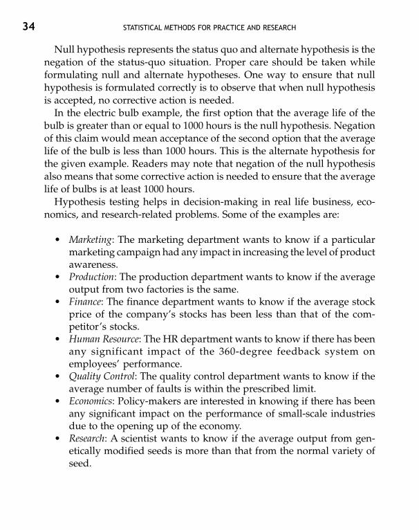
Hypothesis testing helps in decision-making in real life business, eco-nomics, and research-related problems. Some of the examples are:
• Marketing: The marketing department wants to know if a particularmarketing campaign had any impact in increasing the level of productawareness.
• Production: The production department wants to know if the averageoutput from two factories is the same.
• Finance: The finance department wants to know if the average stockprice of the company’s stocks has been less than that of the com-petitor’s stocks.
• Human Resource: The HR department wants to know if there has beenany significant impact of the 360-degree feedback system onemployees’ performance.
• Quality Control: The quality control department wants to know if theaverage number of faults is within the prescribed limit.
• Economics: Policy-makers are interested in knowing if there has beenany significant impact on the performance of small-scale industriesdue to the opening up of the economy.
• Research: A scientist wants to know if the average output from gen-etically modified seeds is more than that from the normal variety ofseed.

BASIC STATISTICAL CONCEPTS 35
2.4.1 Type I and Type II Errors
While testing a hypothesis, if we reject it when it should be accepted, itamounts to Type I error. On the other hand, accepting a hypothesis when itshould be rejected amounts to Type II error. Generally, any attempt to reduceone type of error results in increasing the other type of error. The only wayto reduce both types of errors is to increase the sample size.
2.4.2 Significance Level (p-value)
There is always a probabilistic component involved in the accept–rejectdecision in testing hypothesis. The criterion that is used for accepting orrejecting a null hypothesis is called significance level or p-value.
The p-value represents the probability of concluding (incorrectly) thatthere is a difference in your samples when no true difference exists. It is astatistic calculated by comparing the distribution of a given sample dataand an expected distribution (normal, F, t etc.) and is dependent upon thestatistical test being performed. For example, if two samples are beingcompared in a t-test, a p-value of 0.05 means that there is only a 5% chanceof arriving at the calculated t-value if the samples were not different (fromthe same population). In other words, a p-value of 0.05 means there is onlya 5% chance that you would be wrong in concluding that the populationsare different or 95% confident of making a right decision. For social sciencesresearch, a p-value of 0.05 is generally taken as standard.
2.4.3 One-Tailed and Two-Tailed Tests
A directional hypothesis is tested with a one-tailed test whereas a non-directional hypothesis is tested with a two-tailed test.
The following three relationships are only possible between any twoparameters, µ1 and µ2:
(a) µ1 = µ2
(b) µ1 < µ2
(c) µ1 > µ2

36 STATISTICAL METHODS FOR PRACTICE AND RESEARCH
To be able to formulate mutually exclusive and exhaustive null and alter-native hypotheses from these relations we can choose either (b) or (c) asalternative hypothesis and combine one of these two with (a) to formulatethe null hypothesis. Thus we will have H0 and H1 as:
H0: µ1 ≥ µ2 or µ1 ≤ µ2
H1: µ1 < µ2 or µ1 > µ2
The above hypotheses are called directional hypotheses and one-tailed testsare done for their analysis. If our null hypothesis is given by (a) only and(b) and (c) are combined to formulate alternative hypothesis, we will havethe following H0 and H1:
H0: µ1 = µ2
H1: µ1 ≠ µ2
The above hypotheses are called non-directional, as we are only concernedabout the equality or non-directional inequality of the relationship. A two-tailed test is done for testing such hypotheses.
The null hypothesis is rejected if the p-value obtained is less than andaccepted if it is greater than the significance level at which we are testingthe hypothesis. Most of the times, our objective is to reject the null hypothesisand find support for our alternate hypothesis. Therefore we look for p-valuesto be less than 0.05 (the commonly used significance level).

3
Summarizing Data: Descriptive Statistics
A manager in his day-to-day operations requires as much information aspossible about the business performance, economic environment, and indus-try trends to be able to make the right decisions. With the advancement inthe field of information and communication technologies, it has becomemuch easier to capture data and a huge amount of data is available withthe organizations. However, the sheer amount of data makes it virtuallyimpossible to comprehend it in its raw form. Descriptive statistics are usedto summarize and present this data in a meaningful manner so that theunderlying information is easily understood.
This chapter presents some of the tools for summarizing various kinds ofdata with the help of SPSS and MS Excel. Some basic terms and conceptshave also been briefly explained but the emphasis is in explaining the useof a software package for summarizing data. Readers should refer to somestandard textbook on statistics to get details about the concepts.
3.1 BASIC CONCEPTS
Descriptive statistics are numerical and graphical methods used to sum-marize data and bring forth the underlying information. The numericalmethods include measures of central tendency and measures of variability.

38 STATISTICAL METHODS FOR PRACTICE AND RESEARCH
3.1.1 Measures of Central Tendency
Measures of central tendency provide information about a representativevalue of the data set. Arithmetic mean (simply called the mean), median,and mode are the most common measures of central tendency.
1. Mean or average is the sum of the values of a variable divided bythe number of observations.
2. Median is a point in the data set above and below which half of thecases fall.
3. Mode is the most frequently occurring value in a data set.
Which of the above should be used in a particular case is a judgement call. Forexample, business schools regularly publish the mean salary of their passingout batches every year. However, there may be some outliers in the salarydata on the upper side, which will drive the mean level towards the upperside. Thus in a class of 50 students, if two students manage to get salaries tothe tune of Rs 5 million per annum, and the mean of the remaining 48 stud-ents is 200,000 per annum, the mean of the entire class will be about Rs 400,000per annum, almost double! Clearly, the mean does not tell much about theaverage salary an aspiring student should expect after passing out from theschool. In such a case, the median may be a better measure of central tend-ency. Therefore, only knowing a particular measure of central tendencymay not be sufficient to make any sense of the data as it does not provideany information about the spread of the data. We use measures of variabilityfor this purpose.
3.1.2 Measures of Variability
Measures of variability provide information about the amount of spread ordispersion among the variables. Range, variance, and standard deviationare the common measures of variability.
1. Range is the difference between the largest and the smallest values.2. Variance is the sum of the squared deviations of each value from the
mean divided by the number of observations. Standard deviation isthe positive square root of variance.

SUMMARIZING DATA: DESCRIPTIVE STATISTICS 39
Some other important terms are explained below:
3.1.3 Percentiles, Quartiles, and Interquartile Range
Percentiles and quartiles are used to find the relative standing of values ina data set. The nth percentile is a number such that n% of the values are ator below this number. Median is the 50th percentile or the 2nd quartile.Similarly, the 1st quartile is the 25th percentile and the 3rd quartile is the75th percentile.
Interquartile range is the difference between values at the 3rd quartile(or 75th percentile) and the 1st quartile (or 25th percentile).
3.1.4 Skewness
Besides mean, median, and mode, it is also important to know if the givendistribution is symmetric or not. A distribution is said to be skewed if theobservations above and below the mean are not symmetrically distributed.A zero value of skewness implies a symmetric distribution. The distributionis positively skewed when the mean is greater than the median and nega-tively skewed when the mean is less than the median. Figure 3.1 shows apositively and negatively skewed distribution.
Figure 3.1Negatively and Positively Skewed Distributions

40 STATISTICAL METHODS FOR PRACTICE AND RESEARCH
3.1.5 Kurtosis
Kurtosis is a measure of how peaked or flat a distribution is. A distributioncould be mesokurtic, leptokurtic, or platykurtic.
The absolute value of kurtosis for a mesokurtic or normal distribution is 3;kurtosis for other distributions is always measured relative to this value.Platykurtic distribution has a negative kurtosis, implying a flatter distribu-tion than the normal distribution while leptokurtic distribution has positivekurtosis, implying a more peaked distribution than normal distribution.Figure 3.2 presents a sketch of the above three types of distributions:
Next, we show how to calculate these statistics using the SPSS program.
Figure 3.2Meso, Lepto, and Platykurtic Distributions
3.2 USING SPSS
Example 3.1
A marketing company has a sales staff of 20 sales executives. The data re-garding their age and total sales achieved in their territories in a particularmonth are given in Table 3.1. We wish to calculate some basic descriptivestatistics for this data.

SUMMARIZING DATA: DESCRIPTIVE STATISTICS 41
Table 3.1
Sales Gender SalesExecutives (M=1, F=2) Age Region (in Rs ‘000)
1 1 25 1 502 1 22 1 753 1 20 2 114 1 27 2 775 1 28 3 456 1 24 1 527 1 24 2 268 1 23 3 249 2 24 3 28
10 2 30 3 3111 2 19 2 3612 2 24 1 7213 2 26 1 6914 2 26 1 5115 2 21 2 3416 2 24 2 4017 2 29 3 1818 2 27 3 3519 2 24 1 2920 2 25 1 68
Various options for calculating descriptive statistics can be found in theDescriptive Statistics option under the Analyze menu as shown in Figure 3.3.We will explain their use one by one.
3.2.1 Descriptive Statistics
The first step is to enter the given data in the data editor. The variables arelabeled as executiv, gender, age, region, and sales respectively. Click on Analyze,which will produce a drop down menu, choose Descriptive Statistics fromthat and click on Descriptives as shown in Figure 3.3. The resulting dialogbox is shown in Figure 3.4.
In this dialog box, we have to select the variables for which we wish tocalculate descriptive statistics by transferring them to the Variable(s) box onthe right-hand side from the left-hand side box. For this, first highlight the

42 STATISTICAL METHODS FOR PRACTICE AND RESEARCH
Figure 3.3
Figure 3.4

SUMMARIZING DATA: DESCRIPTIVE STATISTICS 43
variable(s) by clicking on them (the first one—executiv is already high-lighted). Then, click on the arrow button between the two boxes. The high-lighted variable will get transferred to the other box. The same can also bedone by double clicking on the variable, which we wish to transfer. Manydialog boxes for specifying procedures in SPSS in the next chapters will besimilar to this one in many respects.
In our example, we will transfer age and sales to the Variable(s) box forcalculating descriptive statistics about these two. There is a button labeledOption at the right-hand top of the dialog box. Clicking on this will producethe dialog box shown in Figure 3.5.
Figure 3.5
There are some default selections made in this box about the statistics tobe shown in the output. A particular statistic can be selected or deselectedfor display in the output by clicking on the boxes next to their names. Wehave not selected any additional statistics other than what is selected bydefault. Now click on the Continue button to return to the previous dialogbox and then click on OK to run the analysis.

44 STATISTICAL METHODS FOR PRACTICE AND RESEARCH
Output
The output produced is shown in Figure 3.6.
Figure 3.6
The first line tells us about the data set for which descriptive statisticshave been calculated. The first column in the output table, labeled N givesthe number of cases in the data set. In the next two columns, the minimumand maximum value of the variables selected for analysis is given. In thelast two columns, the mean and standard deviation are given.
It can be seen that the age of the sales executives vary from 19 to 30 yearswith a mean age of 24.6 years and a standard deviation of 2.84 years. Simi-larly, the sale achieved varies from Rs 11,000 to Rs 77,000 with a mean salesof Rs 43,550 and a standard deviation of Rs 19,970.
SYNTAX
The syntax for obtaining the above output is given below:
DESCRIPTIVESVARIABLES = age sales/STATISTICS = MEAN STDDEV MIN MAX.
3.2.2 Frequencies
As shown in Figure 3.3, the Frequencies option can be found under Analyzefrom the menu bar. The resulting dialog box is shown in Figure 3.7.
Transfer age from the left-hand side box to the Variable(s) box on the right-hand side for analysis. For transferring variables, first highlight them oneby one by clicking on them. Then click on the arrow button between the twoboxes to transfer the highlighted variable to the other box. Here, we haveselected only age for illustration.
SUMMARIZING DATA: DESCRIPTIVE STATISTICS 45
Figure 3.7
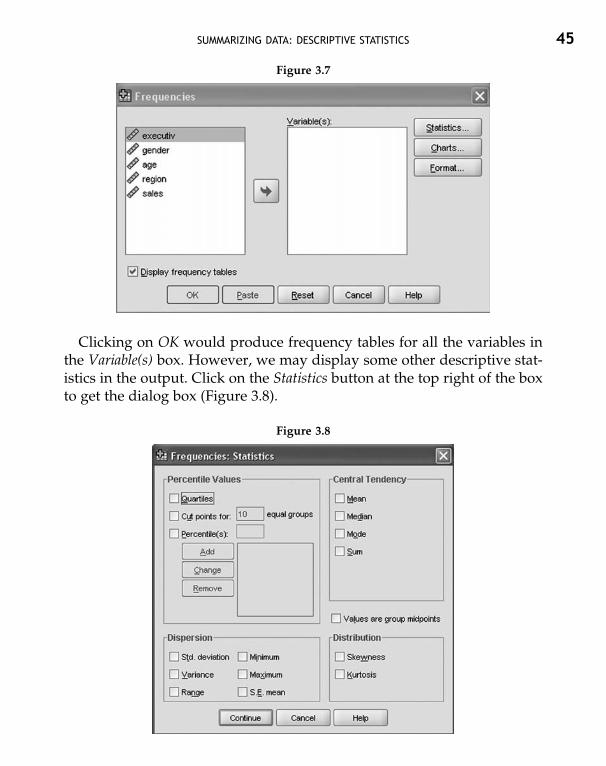
Clicking on OK would produce frequency tables for all the variables inthe Variable(s) box. However, we may display some other descriptive stat-istics in the output. Click on the Statistics button at the top right of the boxto get the dialog box (Figure 3.8).
Figure 3.8

46 STATISTICAL METHODS FOR PRACTICE AND RESEARCH
There are a variety of descriptive statistics mentioned in this dialog boxunder four categories—percentile values, central tendency, dispersion, anddistribution. All the statistics under central tendency, dispersion, and dis-tribution categories are selected for analyses here. Besides the statistics underthe four categories, there is an option for selection by the name Values aregroup midpoints. This is for grouped data and need not be selected in ourexample.
Now, click on Continue to return to the previous dialog box. At this stage,we can run the analysis by clicking on OK or opt for a graphical display offrequency distribution. For a graphical display, click on the Charts button;this will produce a dialog box as shown in Figure 3.9.
Figure 3.9
Select the type of chart you wish to show in the output and click on Con-tinue to return to the main dialog box. For our example, we have opted forbar charts since the variables under study have only small number of values.For variables with large number of values, histograms are preferred. Clickon OK on the main dialog box to run the analysis.
Output
The output produced is shown in three heads—frequencies, frequency table,and bar chart in Figures 3.10, 3.11, and 3.12 respectively.

SUMMARIZING DATA: DESCRIPTIVE STATISTICS 47
SPSS output produces all the descriptive statistics requested for the se-lected variables as shown in Figure 3.10. The details about these statisticshave been given at the beginning of the chapter. It also produces frequencydistribution for each variable. In Figure 3.11, we have shown the frequencydistribution output only for Age. The first column of the frequency tablelists all the values found for the variable; the second column titled Frequencylists the number of data points having that value; the third column titledPercent gives the percentage of all data points having that particular value;the fourth column titled Valid Percent gives the percentage of all valid datapoints on this variable; and the fifth column gives the cumulative percentagefor that value.
Figure 3.12 shows the bar chart of the output for the variable Age. On thehorizontal axis are shown the values and on the vertical axis, their fre-quencies. Much advanced graphical display of data can be done in SPSSunder the Graphs option from the menu bar.
Figure 3.10

48 STATISTICAL METHODS FOR PRACTICE AND RESEARCH
Figure 3.11
Figure 3.12

SUMMARIZING DATA: DESCRIPTIVE STATISTICS 49
SYNTAX
The syntax for obtaining the above output is given below:
FREQUENCIESVARIABLES = age/STATISTICS = STDDEV VARIANCE RANGE MINIMUMMAXIMUM SEMEAN MEAN MEDIAN MODESUM SKEWNESS SESKEW KURTOSIS SEKURT/BARCHART FREQ/ORDER = ANALYSIS.
3.2.3 Tables
We cannot obtain descriptive statistics for different groups of variables usingeither Descriptives or Frequencies. For example, in the above case if want tofind out the descriptive statistics for the male and female sales executives,we have to split the file which can be done from the data menu. However,the tables command can still be used to produce descriptive statistics brokendown by one or more categorical variables.
The option to obtain tables is not available under the Analyze menu inSPSS 16.0. However, one can get this feature as an add-on to the basepackage. In SPSS 14, and earlier versions, one can obtain tables followingthe procedure given below.
From the menu bar, click on Analyze and select Basic tables from the Tablesoption. The resulting dialog box is shown in Figure 3.13.
Select the variable for which you want to produce the descriptive statisticsand transfer into the box labeled Summaries. There are three more boxeslabeled Down, Across, and Separate Tables below Summaries in Figure 3.13.The categorical variables by which the groups are to be formed, have to bemoved to one of these boxes. Which box to choose for moving the groupingvariable will depend on the way you want your tables to be produced. TheDown option will produce a separate row whereas the Across option willproduce a separate column for each level of the categorical variable. TheSeparate Tables option will produce a separate table for each level of the cat-egorical variable.
In this example we transfer age to the box labeled Summaries and genderto the box labeled Down. Readers are encouraged to explore other options.Click on the button labeled Statistics. This will produce a dialog box labeledBasic Tables: Statistics (Figure 3.14).

50 STATISTICAL METHODS FOR PRACTICE AND RESEARCH
Figure 3.13
Figure 3.14

SUMMARIZING DATA: DESCRIPTIVE STATISTICS 51
Select the statistics you want for the data from the box labeled Statisticson the left-hand side. Selecting any one statistic will turn the button labeledAdd active. Click on Add to transfer the required statistic to the box labeledCell Statistics. You can remove a particular statistic from this box by clickingon the Remove button, which becomes active only when there is at least onestatistic transferred to the Cell Statistics box. For our example, we will chooseMaximum, Mean, Median, Minimum, and Mode. There are a variety of otheroptions on these dialog boxes by which one can choose the layout and ap-pearance of the output. Readers are encouraged to experiment with theseoptions and discover how they work. Click on Continue to return to the pre-vious dialog box and click on OK to run the analysis.
Output
The output produced is shown in Figure 3.15. It is self explanatory.
Figure 3.15
SYNTAX
The syntax for obtaining the above output is given below:
TABLES/FORMAT BLANK MISSING(‘.’)/OBSERVATION age/TABLES gender > ageBY (STATISTICS)/STATISTICSmaximum( )mean( )median( )minimum( )mode( ).

4
Comparing Means:
One or Two Samples t-Tests
t-tests and z-tests are commonly used when making comparisons betweenthe means of two samples or between some standard value and the meanof one sample. There are different varieties of t-tests which are used in dif-ferent conditions depending on the design of the experiment or the natureof the data. These are explained in detail in the following sections.
4.1 BASIC CONCEPTS
4.1.1 t-test and z-test
t-tests are similar to commonly encountered z-tests in many ways. Bothz- and t-tests have the same rationale but use different assumptions, whichrequire a careful selection depending on the requirements. For z-tests, thepopulation mean and population standard deviation should be knownexactly. In many real life problems, while the population mean is known, theexact population standard deviation cannot be calculated. In such cases,t-tests should be used. Besides, the t-test does not require a big sample size.Most statisticians feel that with a sample size of 30–40, results of the t-testare very close to those obtained from the z-test.
There are three different types of t-tests: one sample t-test, independentsamples t-test, and dependent (paired) samples t-test. Each of these is ex-plained further.

COMPARING MEANS: ONE OR TWO SAMPLES t-TESTS 53
4.1.2 One Sample t-test
One sample t-test is used to compare the mean of a single sample with thepopulation mean. Some situations where one sample t-test can be used aregiven below:
• An economist wants to know if the per capita income of a particularregion is same as the national average.
• A market researcher wants to know if the proposed product will beable to penetrate to a certain level in the households in order to makeits introduction profitable.
• The Quality Control department wants to know if the mean dimensionsof a particular product have shifted significantly away from the ori-ginal specifications.
4.1.3 Independent Samples t-test
In many real life situations, we cannot determine the exact value of thepopulation mean. We are only interested in comparing two populationsusing a random sample from each. Such experiments, where we are inter-ested in detecting differences between the means of two independent groupsare called independent samples test. Some situations where independentsamples t-test can be used are given below:
• An economist wants to compare the per capita income of two differentregions.
• A market researcher wants to know in which territory will his productbe able to penetrate more. This will help him in deciding the rightplace to introduce the product.
• A labor union wants to compare the productivity levels of workersfor two different groups.
• An aspiring MBA student wants to compare the salaries offered to thegraduates of two business schools.
In all the above examples, the purpose is to compare between two inde-pendent groups in contrast to determining if the mean of the group exceedsa specific value as in the case of one sample t-tests.

54 STATISTICAL METHODS FOR PRACTICE AND RESEARCH
4.1.4 Dependent (Paired) Samples t-test
In case of independent samples test for testing the difference between means,we assume that the observations on one sample are not dependent on theother. However, this assumption limits the scope of analysis as in manycases the study has to be done on the same set of elements (people, objectsetc.) to control some of the sample specific extraneous factors. Such experi-ments where the observations are made on the same sample at two differenttimes, is called dependent or paired sample t-test. Some situations wheredependent samples t-test can be used are given below:
• The HR manager wants to know if a particular training program hadany impact in increasing the motivation level of the employees.
• The production manager wants to know if a new method of handlingmachines helps in reducing the break down period.
• An educationist wants to know if interactive teaching helps studentslearn more as compared to one-way lecturing.
One can compare these cases with the previous ones to observe the dif-ference. The subjects in all these cases are the same and observations aretaken at two different times.
4.2 USING SPSS
Various options for different types of t-tests can be found in the CompareMeans option under the Analyze menu as shown in Figure 4.1. We will explainthe procedure for the three types of t-tests one by one.
4.2.1 One Sample t-test
Example 4.1
A business school in its advertisements claims that the average salary of itsgraduates in a particular lean year is at par with the average salaries offeredat the top five business schools. A sample of 30 graduates, from the businessschool whose claim was to be verified, was taken at random. Their salariesare given in Table 4.1.

COMPARING MEANS: ONE OR TWO SAMPLES t-TESTS 55
Table 4.1
Graduate Salary Graduate SalaryStudent (in Rs ‘000) Student (in Rs ‘000)
1 750 16 7702 600 17 6803 600 18 6704 650 19 7405 700 20 7606 780 21 7757 860 22 8458 810 23 8709 780 24 640
10 670 25 69011 690 26 71512 550 27 63013 610 28 68514 715 29 78015 755 30 635
Figure 4.1

56 STATISTICAL METHODS FOR PRACTICE AND RESEARCH
The average salary offered at the top five business schools in that yearwas given as Rs 750,000.
In this problem we want to assess validity of the claim made by thebusiness school in its advertisements. We want to know if the average salaryof the business school is significantly different from Rs 750,000, the averagesalary at the top five business schools for that particular year. The nullhypothesis would be:
H0: There is no difference between the average salary of the businessschool in question and the average salary of the top five business schools.
As explained earlier, the first step is to enter the given data in the dataeditor. The variables are labeled as student and salary respectively. Click onAnalyze, which will produce a drop down menu, choose Compare Meansfrom that and click on One-Sample T Test... as shown in Figure 4.1. The result-ing dialog box is shown in Figure 4.2.
Figure 4.2
The variables can be selected for analysis by transferring them to the TestVariable(s) box on the right-hand side. Next, change the value in the Test Valuebox, which originally appears as 0, to the one against which you are testingthe sample mean. In this case, this value would be 750 (not 750,000, sinceother salary figures are also in ‘000). Now click on OK to run the analysis.

COMPARING MEANS: ONE OR TWO SAMPLES t-TESTS 57
Output
The output produced is shown in Figure 4.3.
Figure 4.3
The first table, labeled One-Sample Statistics, gives descriptive statisticsfor the variable salary. The second table, labeled One-Sample Test, gives theresults of the t-test analysis. The first entry is the value of the t-statistic,next is the degrees of freedom (df), followed by the corresponding p valuefor 2-tailed test given as Sig. (2-tailed).
The test result gives the t-statistic of –2.46 with 29 degrees of freedom.The corresponding two-tailed p value is 0.02. If we take the significancelevel of 5%, we can see that the p value obtained is less than 0.05. Therefore,we can reject the null hypothesis at α = 0.05, which means that the samplemean is significantly different from the hypothesized value and the aver-age salary of the business school in question is not the same as the averagesalary of the top five business schools at the 5% level of significance.
However, at α = 0.01 the null hypothesis will have to be accepted sincethe p-value is greater than 0.01. This means that at 1% level of significance,the claim of the business school that its salaries are same as that of the topfive business schools is right.
The second output window also gives the mean difference (the differencebetween sample mean and the hypothesized value) and the interval limitsat the specified values of the confidence level. These figures are not of muchuse for practical considerations.
58 STATISTICAL METHODS FOR PRACTICE AND RESEARCH
SPSS does not give the one-tailed significance value directly, however, onecan compute the one-tailed value by dividing the two-tailed value by 2.
SYNTAX
The syntax for obtaining the above output is given below:
T-TEST/TESTVAL=750/MISSING=ANALYSIS/VARIABLES=salary/CRITERIA=CIN (.95).
4.2.2 Independent Samples t-test
Example 4.2
A study was conducted to compare the efficiency of the workers of two mines,one with private ownership and the other with government ownership.The researcher was of the view that there is no significant difference intheir efficiency levels. Total tonnage of the mineral mined by a worker inone shift was chosen as the criteria to assess his efficiency.
Twenty workers from the private sector mine and 24 from the government-owned mine were selected and their average output per shift was recorded.The data obtained is given in Table 4.2.
In this problem we want to assess whether the efficiency of the workersof the two mines is the same. The null hypothesis in this case would be thatthere is no difference in the efficiency of the workers of the two mines.
H0: Average output of the workers from mine 1 equals that of theworkers from mine 2.
The alternative hypothesis in this case would be that the workers of the twomines significantly differ in their efficiency, i.e., average output of workersof mine 1 is significantly different from that of the workers of mine 2.
The variables are labeled as miner, mine, and output respectively for enter-ing into the SPSS Program. Click on Analyze, which will produce a drop downmenu, choose Compare Means from that and click on Independent-SamplesT Test as shown in Figure 4.1. The resultant dialog box is shown in Figure 4.4.

COMPARING MEANS: ONE OR TWO SAMPLES t-TESTS 59
Table 4.2
Output OutputMiner Mine (in tons) Miner Mine (in tons)
1 1 48 23 2 412 1 45 24 2 393 1 33 25 2 354 1 39 26 2 345 1 34 27 2 336 1 49 28 2 367 1 33 29 2 378 1 45 30 2 379 1 48 31 2 41
10 1 44 32 2 4211 1 45 33 2 3912 1 45 34 2 3813 1 36 35 2 3814 1 48 36 2 3915 1 41 37 2 4116 1 47 38 2 4017 1 39 39 2 4118 1 49 40 2 4019 1 38 41 2 3820 1 45 42 2 4121 2 42 43 2 4322 2 44 44 2 40
Figure 4.4

60 STATISTICAL METHODS FOR PRACTICE AND RESEARCH
Initially all the variables are shown in the left-hand box. To perform theIndependent-Samples t-test, transfer the dependent variable(s) into the TestVariable(s) box and transfer the variable that identifies the groups into theGrouping Variable box. In this case output is the dependent variable to beanalyzed and should be transferred into Test Variable(s) box by clicking onthe first arrow in the middle of the two boxes. Mine is the variable whichwill identify the groups of the miners and it should be transferred into theGrouping Variable box.
Once the Grouping Variable is transferred, the Define Groups button whichwas earlier inactive turns active. Clicking on it will produce a box shown inFigure 4.5.
Figure 4.5
In the example Group 1 represents the miners of mine 1 and Group 2represents the miners of mine 2, which we have entered under the variablemine in the data editor. Therefore, put 1 in the box against Group 1, put 2in the box against Group 2, and click Continue. Now click on OK to runthe test.
Output
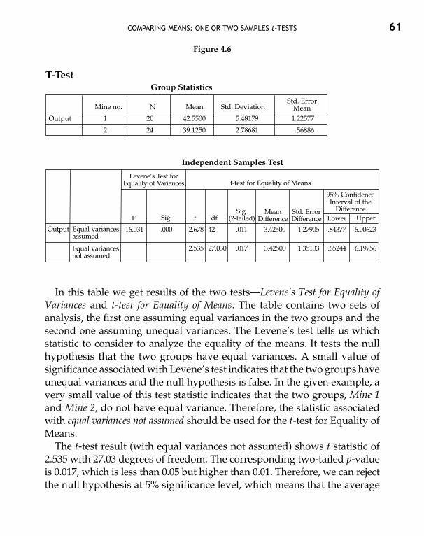
The output produced is shown in Figure 4.6The first table, labeled Group Statistics gives descriptive statistics (number
of data sets, means, standard deviations, and standard errors of means) forboth the groups. The second table labeled Independent-Samples Test givesthe results of the analysis.
COMPARING MEANS: ONE OR TWO SAMPLES t-TESTS 61
In this table we get results of the two tests—Levene’s Test for Equality ofVariances and t-test for Equality of Means. The table contains two sets ofanalysis, the first one assuming equal variances in the two groups and thesecond one assuming unequal variances. The Levene’s test tells us whichstatistic to consider to analyze the equality of the means. It tests the nullhypothesis that the two groups have equal variances. A small value ofsignificance associated with Levene’s test indicates that the two groups haveunequal variances and the null hypothesis is false. In the given example, avery small value of this test statistic indicates that the two groups, Mine 1and Mine 2, do not have equal variance. Therefore, the statistic associatedwith equal variances not assumed should be used for the t-test for Equality ofMeans.
The t-test result (with equal variances not assumed) shows t statistic of2.535 with 27.03 degrees of freedom. The corresponding two-tailed p-valueis 0.017, which is less than 0.05 but higher than 0.01. Therefore, we can rejectthe null hypothesis at 5% significance level, which means that the average
Figure 4.6

62 STATISTICAL METHODS FOR PRACTICE AND RESEARCH
outputs of the two mines are significantly different from each other, i.e.,the miners of the two mines do not have the same efficiency. However at1% significance level, the null hypothesis will have to be accepted since thep-value is greater than 0.01. This means that at 1% significance level, theclaim that the efficiency of the miners of the two mines is same is right.
The table also gives the mean difference, i.e., the difference between theaverage daily output by the workers of mine 1 and mine 2, standard errorof difference, and 95% confidence interval of the difference. While the meandifference helps in observing the total amount of difference between themean values for the two groups, the other two values are not of much im-portance for practical purposes.
One-tailed and Two-tailed Tests
We may recall the hypotheses we tested above:
H0: O1 = O2H1: O1 ≠ O2
Here we are only interested in knowing if the efficiency of the workers ofmine 1 is same as that of the workers of mine 2. The appropriate test for thiswould be a two-tailed test. However, if we were to test the assumption thatthe efficiency of workers of mine 1 is greater than that of the workers ofmine 2, the null and alternative hypotheses would be different and we wouldneed the p-value of one-tailed test. The new hypotheses would be:
H0: O1≤ O2H1: O1 > O2
The one-tailed significance value or p-value can be obtained by dividingthe two-tailed value by two. Thus the one-tailed p-value in this case wouldbe 0.0085, which is less than 0.01. Therefore we reject the null hypothesiseven at 1% significance level and conclude that the efficiency of the workersof mine 1 is greater than that of the workers of mine 2.

COMPARING MEANS: ONE OR TWO SAMPLES t-TESTS 63
SYNTAX
The syntax for obtaining the above output is given below:
T-TESTGROUPS=mine(1 2)/MISSING=ANALYSIS/VARIABLES=output/CRITERIA=CIN(.95).
4.2.3 Dependent Samples t-test
Example 4.3
A corporate training institution claimed that its training program can greatlyenhance the efficiency of call center employees. A big call center sent someof its employees for the training program. The efficiency was measured bythe number of deals closed by each employee in a one-month period. Datawas collected for a one-month period before sending the employees for thetraining program. After the training program, data was again collected onthe same employees for a one-month period. The data is given in Table 4.3.
Table 4.3
Before the After the Before the After theTraining Training Training Training
Employee Program Program Employee Program Program
1 41 44 11 46 392 35 36 12 42 403 40 48 13 37 364 50 47 14 34 395 39 40 15 38 506 45 52 16 42 467 35 35 17 46 498 36 51 18 39 429 44 46 19 40 51
10 40 55 20 45 37

64 STATISTICAL METHODS FOR PRACTICE AND RESEARCH
In this problem, we want to test the validity of the claim made by thetraining institution that its training program improves the efficiency of callcenter employees. We want to know if there is a significant difference inthe average output of the employees before and after going through thetraining program.
The null hypothesis here would be that the average output of the em-ployees is same before and after going through the training program.
The given data is entered in the data editor and the variables are labeledas employee, before, and after respectively. Click on Analyze, which willproduce a drop down menu, choose Compare Means from that and click onPaired-Samples T Test as shown in Figure 4.1. The resulting dialog box isshown in Figure 4.7.
Figure 4.7
The variables appear in the left-hand box. From this box we have to selectthe variables, which are to be compared. The two variables to be comparedin our case are before and after. Select these variables one by one, and clickon the arrow between the two boxes to transfer them to the Paired Variablesbox. We can compare more than one pair in the same analysis. Now clickon OK to run the analysis.
COMPARING MEANS: ONE OR TWO SAMPLES t-TESTS 65
Output
The output produced is shown in Figure 4.8 in three tables. The first tablelabeled Paired Samples Statistics gives descriptive statistics (means, numberof data sets, standard deviations, and standard errors of means) for bothbefore and after situations. The second table labeled Paired Samples Correlationsgives the value of the correlation coefficient between the two variables andsignificance level for the two-tailed test to assess the hypothesis that the cor-relation coefficient equals zero. This has been explained in detail in Chapter 7.
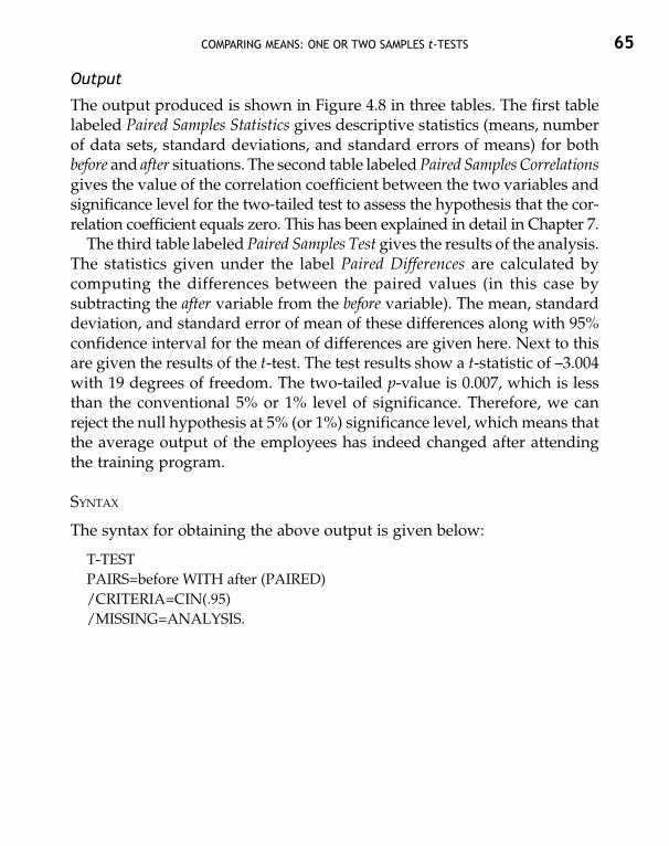
The third table labeled Paired Samples Test gives the results of the analysis.The statistics given under the label Paired Differences are calculated bycomputing the differences between the paired values (in this case bysubtracting the after variable from the before variable). The mean, standarddeviation, and standard error of mean of these differences along with 95%confidence interval for the mean of differences are given here. Next to thisare given the results of the t-test. The test results show a t-statistic of –3.004with 19 degrees of freedom. The two-tailed p-value is 0.007, which is lessthan the conventional 5% or 1% level of significance. Therefore, we canreject the null hypothesis at 5% (or 1%) significance level, which means thatthe average output of the employees has indeed changed after attendingthe training program.
SYNTAX
The syntax for obtaining the above output is given below:
T-TESTPAIRS=before WITH after (PAIRED)/CRITERIA=CIN(.95)/MISSING=ANALYSIS.

66 STATISTICAL METHODS FOR PRACTICE AND RESEARCH
Figu
re 4
.8

5
Comparing Means: Analysis of Variance
ANOVA or Analysis of Variance is used to compare the means of more thantwo populations. It uncovers the main and interaction effects of classificationor independent variables on one or more dependent variables. ANOVA hasfound extensive application in psychological research using experimentaldata. It can also be used in business management, especially in consumerbehavior and marketing management related problems. The examples givenbelow will help in understanding the applicability of ANOVA for solvingpractical problems:
• Consumer behavior: A researcher wants to investigate the impact of threedifferent advertising stimuli on the shopping propensity of males andfemales as well as consumers of different age brackets. The dependentvariable here is shopping propensity and independent variables orthe factors are advertising stimuli, gender, and age brackets.
• Marketing management: A marketing manager wants to investigate theimpact of different discount schemes on the sale of three major brandsof edible oil.
• Social sciences: A social scientist wants to predict whether the effect-iveness of an AIDS awareness campaign varies depending on thegeographic location, campaign media, and usage of celebrities in thecampaigns.
5.1 BASIC CONCEPTS
5.1.1 ANOVA Procedure
ANOVA analysis uses the F-statistic, which tests if the means of the groups,formed by one independent variable or a combination of independent

68 STATISTICAL METHODS FOR PRACTICE AND RESEARCH
variables, are significantly different. It is based on the comparison of twoestimates of variances—one representing the variance within groups, oftenreferred to as error variance and the other representing the variance due todifferences in group means. If the two variances do not differ significantly,one can believe that all the group means come from the same sampling dis-tribution of means and there is no reason to claim that the group meansdiffer. If, however, the group means differ more than can be accountedfor due to random error, there is reason to believe that they were drawnfrom different sampling distributions of means. The F-statistic calculatesthe ratio between the variance due to difference between groups and theerror variance.
F = Variance due to difference between groups/Error variance
The larger the F-ratio, the greater is the difference between groups as com-pared to within group differences. An F-ratio equal to or less than 1 indicatesthat there is no significant difference between groups and the null hypothesisis correct. If the null hypothesis (that the group means do not differ signifi-cantly) is correct, then we can conclude that the independent variables didnot have an effect on the dependent variable. However, if the F-test provesthe null hypothesis to be wrong, multiple comparison tests are used to fur-ther explore the specific relationships among different groups.
The ANOVA procedure can be used correctly if the following conditionsare satisfied:
1. The dependent variable should be interval or ratio data type.2. The populations should be normally distributed and the population
variances should be equal.
5.1.2 Factors and Covariates
Factors are independent variables because of which the groups might dif-fer significantly. There could be just one factor or more than one factor in anANOVA analysis. The analysis, however, is very cumbersome as will beclear later in the chapter, if the number of factors goes beyond three to four.A factor may have many levels.
Factors could be fixed or random. A factor is fixed if it contains all thelevels of interest and random if the levels under study are a random sample

COMPARING MEANS: ANALYSIS OF VARIANCE 69
of the possible levels that could be sampled and the goal is to make a state-ment regarding the larger population.
Covariates are interval-level independent variables. By entering covariatesin the model, we can remove the effects of the relationship between thecovariate and the dependent variable and get a more precise estimate ofthe amount of variance by the factors in the model.
5.1.3 Between, Within, and Mixed (Between-Within) Designs
An ANOVA design can be described by specifying three things:
1. Number of factors involved in the design.2. Number of levels of each of the factors.3. Whether the factor is a between- or within-subjects factor.
In between-groups design, the level of factor(s) varies between the subjectsof different groups so that the subjects of each group will be exposed toonly one level of the factor(s). This design is conceptually similar to the inde-pendent sample design discussed in the case of t-tests.
In within-groups design, the level of factor(s) varies within the subjects.This is done by exposing the same subject to different levels of the factor(s)at different times. It is also referred as repeated measures design. This designis conceptually similar to the paired sample design discussed in the case oft-tests.
When there are both, between-groups as well as within-groups factorspresent in a design, it is referred to as mixed design.
5.1.4 Main Effects and Interactions
Main effect is the direct effect of a single factor or independent variable onthe dependent variable. It simply compares the mean of one level of a factorwith the other level(s) of that factor. Interaction effect is the combined effectof two or more factors on the dependent variable.
ANOVA designs are sometimes classified depending on the number offactors. Thus a one-way ANOVA includes a single factor which gives riseto a single main effect. In case of a two-way ANOVA, there are two maineffects of two factors and one two-way interaction effect between the two

70 STATISTICAL METHODS FOR PRACTICE AND RESEARCH
factors. Likewise, in the case of a three-way ANOVA, there are three maineffects of three factors, three two-way interactions, and one three-way inter-action. If the three factors in three-way ANOVA are X, Y, and Z, then we willhave three main effects of X, Y, and Z, three two-way interactions X*Y, X*Zand Y*Z, and one three-way interaction X*Y*Z.
As the number of factors increase in an ANOVA design, the number ofinteractions increases steeply. In case of a four-way ANOVA, there are fourmain effects, six two-way interactions, four three-way interactions, and onefour-way interaction. Thus the researcher has to analyze a total of 15 results.For this reason, it is not easy to interpret results of ANOVA involving morethan three to four factors. Beginners are advised to keep their experimentaldesigns simple so as not to have more than four factors.
5.1.5 Post-Hoc Multiple Comparisons
Rejection of the null hypothesis in ANOVA only tells us that all populationmeans are not equal. Multiple comparisons are used to assess which groupmeans differ from which others, once the overall F-test shows that at leastone difference exists. Many tests are listed under “Post-Hoc” in SPSS. TukeyHSD (honestly significant difference) test is one of the most conservativeand commonly used test and has been explained in the examples given inthis chapter.
5.1.6 Contrast Analysis
Contrasts are also used to do multiple comparisons in ANOVA. Using con-trasts, we may test the significance of specific differences in particular partsof the design, like testing the differences between two particular means orcomparing the average of a combination of means to a particular mean.This has also been explained later in the examples.
5.2 USING SPSS
As explained earlier, one may have many ANOVA designs depending onthe number of factors and levels of these factors. In the following section,

COMPARING MEANS: ANALYSIS OF VARIANCE 71
we will show how to use SPSS to solve the following two basic ANOVAdesigns:
One-Way Between-Groups ANOVATwo-Way Between-Groups ANOVA
The SPSS program has the following four options for carrying out theANOVA analysis:
One-Way ANOVAUnivariate GLMMultivariate GLMRepeated Measure GLM
One-Way ANOVA is the generalization of the t-test for independent samplesto situations with more than two groups. It is also known as single clas-sification ANOVA or one-factor ANOVA. It is used to test the difference ina single dependent variable among two or more groups formed by a singleindependent or classification variable. It can be found under the CompareMeans item in the Analyze menu by the name One-Way ANOVA.
The other three techniques, viz., univariate, multivariate, and repeatedmeasures are found under the General Linear Model in the Analyze menu.The Univariate GLM is used to assess the main and interaction effects ofseveral independent variables on a single dependent variable. The inde-pendent variables could be fixed factors, random factors, or covariates. TheMultivariate GLM is used when we have more than one dependent variableand several independent variables. This design is also known as MANOVA.The Repeated Measures GLM is used when a dependent variable is meas-ured repeatedly across a set of conditions for all the subjects of the sample.Thus it is a generalization of the t-test for paired samples.
5.2.1 One-Way Between-Groups ANOVA
This analysis can be carried out in two ways in SPSS—using One-WayANOVA or using Univariate GLM. The following example has been solvedusing both methods.

72 STATISTICAL METHODS FOR PRACTICE AND RESEARCH
Example 5.1
An oil company has introduced a new brand of gasoline in its outlets inthree major metro cities. However, they are not sure how the new brand isselling at the three places since there is a lot of difference in the driving habitsof people in the three metros. The company selected 10 outlets in each cityand tabulated the data on an average daily sale at each of the selected outlets.The data is presented in Table 5.1. The items 1, 2, and 3 in the table representthe three metros.
Table 5.1
Volume Volume Volume Outlets Metro (in Gallon) Outlets Metro (in Gallon) Outlets Metro (in Gallon)
1 1 15.00 11 2 8.00 21 3 14.602 1 13.50 12 2 8.25 22 3 16.503 1 14.20 13 2 6.40 23 3 13.204 1 13.00 14 2 7.20 24 3 13.605 1 15.00 15 2 4.40 25 3 21.006 1 11.00 16 2 11.30 26 3 11.707 1 12.50 17 2 7.80 27 3 12.308 1 16.00 18 2 8.10 28 3 17.009 1 14.25 19 2 9.00 29 3 14.75
10 1 13.50 20 2 6.80 30 3 18.00
The null hypothesis in this case is:
H01: The average sale of the new brand of gasoline is same in all themetro cities.
We will also explain multiple comparisons in this example by testing forthe following null hypotheses:
H02: The average sale of the new brand of gasoline in city 1 is same asthat in city 2.H03: The average sale of the new brand of gasoline in city 1 is same asthat in city 2 and city 3 together.
Please note the difference between H02, H03, and H01. The F-statistics obtainedfrom ANOVA only tells us whether there is any significant difference in the

COMPARING MEANS: ANALYSIS OF VARIANCE 73
mean values of the three groups, which is our H01. From this, we cannotconclude anything about specific hypotheses as stated in H02 and H03.The later two hypotheses can be tested using multiple comparisons, whichhave been explained in the last section.
Using One-Way ANOVA
As explained in Chapter 1, first the given data is entered in the data editor.The variables are labeled as outlets, metro, and volume respectively. Click onAnalyze, which will produce a drop down menu, choose Compare Meansfrom that and click on One-Way ANOVA. The resulting dialog box is shownin Figure 5.1.
Figure 5.1
Initially, all the variables are shown in the left-hand box. To perform One-Way ANOVA, transfer the dependent variable into the box labeled Depend-ent List and the factoring variable into the box labeled Factor. In this caseVolume is the dependent variable and should be transferred into theDependent List box by clicking on the first arrow in the middle of the twoboxes. Metro is the factoring variable and should be transferred into Factorbox by clicking on the second arrow. One can select a number of additionalstatistics from Options, depending on specific requirements. The dialog boxobtained by clicking on Options is shown in Figure 5.3 and explained alongwith Options available in Univariate GLM.

74 STATISTICAL METHODS FOR PRACTICE AND RESEARCH
Using Univariate GLM Command
Click on Analyze, which will produce a drop down menu, choose GeneralLinear Model from that and click on Univariate. The resulting dialog box isshown in Figure 5.2.
Figure 5.2
Transfer the dependent variable (volume) into the Dependent variablebox and the factoring variable (metro) into the Fixed Factor(s) box. Click onOptions to ask for additional statistics. The dialog box obtained by clickingon Options is shown in Figure 5.4.
Statistically, random factors are those variables whose levels are assumedto be randomly selected from an infinite population of possible levels. Fixedfactors, on the other hand, contain all of the levels of a particular variable.For example, the gender of a person could be a fixed factor if one believes

COMPARING MEANS: ANALYSIS OF VARIANCE 75
Figure 5.3
Figure 5.4

76 STATISTICAL METHODS FOR PRACTICE AND RESEARCH
male and female to be exhaustive categories specifying gender. Age bracketor income, on the other hand is a random factor as age/income brackets maynot contain exhaustive categories. The choice between random factors andfixed factors may vary depending on the research design.
One can get descriptive statistics of the data by clicking on the box oppositeDescriptive in Figure 5.3 and Descriptive statistics in Figure 5.4. Clicking onEstimates of effect size in Figure 5.4 will give the eta-squared statistic. Thisgives the proportion of total variance accounted for by the factor. This is animportant advantage of using Univariate GLM command as one cannotobtain estimates of effect sizes using One-Way ANOVA command. One-WayANOVA command, however, does have the advantage of a much simpleroutput. Click on Continue and click on OK to run the analysis.
Output for One-Way ANOVA
The output for One-Way ANOVA is shown in Figure 5.5 labeled Oneway.
Figure 5.5
The table, labeled Oneway gives the result of the analysis for an omnibushypothesis. The results are given in three rows. The first row labeled BetweenGroups gives the variability due to the place of sale (between-groups vari-ability), the second row labeled Within Groups gives variability due torandom error, and the third row gives the total variability. In the given ex-ample, F-value is 35.524 and the corresponding p-value is given as <0.000.Therefore we can safely reject the null hypothesis (H01) and conclude thatthe average sale of the new brand of gasoline is not the same in all threemetros.

COMPARING MEANS: ANALYSIS OF VARIANCE 77
The results will be reported as:
There is a significant difference in the sales volume of the new brandof gasoline in the three metros, F (2, 27) = 35.52, p < 0.001.
SYNTAX
The syntax for obtaining the above output is given below:
ONEWAYvolume BY metro/MISSING ANALYSIS.
Output for Univariate GLM
The output for Univariate GLM is shown in Figure 5.6 labeled UnivariateAnalysis of Variance.
Figure 5.6
aR Squared = .725 (Adjusted R Squared = .704).

78 STATISTICAL METHODS FOR PRACTICE AND RESEARCH
The first table labeled Between-Subjects Factors gives the number of subjectsin each level of the factor.
The second table labeled Tests of Between-Subjects Effects gives the ANOVAresults. The first column lists the various sources of variance. The secondcolumn gives the sum of squares of each source of variance. The F-valueand corresponding degrees of freedom are listed in the fifth and thirdcolumns respectively. The column labeled Mean Square gives the meansquare of each source of variance. The last column labeled Partial Eta Squaredis obtained if we select Estimates of effect size from the options and it representsthe size of the effect.
For the given example, the values to be paid attention to are the F-ratio,df, and p-value corresponding to the classification variable (factor) Metro,and the df corresponding to the error term.
The results will be reported in the same manner as in the case of One-WayANOVA output. The 0.725 value of partial eta squared tells us that Metroaccounts for 72.5% of the total variance in Volume.
SYNTAX
The syntax for obtaining the above output is given below:
UNIANOVAvolume BY metro/METHOD = SSTYPE(3)/INTERCEPT = INCLUDE/PRINT = ETASQ/CRITERIA = ALPHA(.05)/DESIGN = metro.
5.2.2 Unplanned and Planned Comparisons
The F-statistic in ANOVA only tells us that the dependent variable variesfor different levels of factor(s). In case of more than two levels, the F-statisticdoes not tell us the exact way in which the dependent variable differs bythe levels of factor(s). To gain a deeper understanding of the subject, wehave to rely on unplanned and planned comparisons.

COMPARING MEANS: ANALYSIS OF VARIANCE 79
By unplanned comparisons, we mean exploring the differences in meansbetween all possible pairs of groups. In the example given above, an un-planned comparison would mean that the researcher is interested in iden-tifying whether the average sale of gasoline in a particular city is differentfrom any other city. While making such comparisons, the researcher hasno a priori hypotheses about differences in the dependent variable for dif-ferent levels of the factor(s). Post-Hoc tests are used for such unplannedcomparison.
Planned comparisons, on the other hand, are decided a priori by the re-searcher, based on theoretical considerations. Such comparisons can be doneusing the Contrasts analysis. A common and most frequently used techniqueis to use a linear combination of contrasts. The method of assigning weightsis very simple and can be learned easily with little practice.
For Example 5.1, we had three null hypotheses. We tested the first ofthese (H01) using the F-statistic as illustrated earlier. The other two (H02 andH03) are based on planned comparisons. For H02, the contrasts coefficientswill be –1, 1, and 0 for city 1, 2, and 3 respectively. This assignment comparesthe mean for city 1 with the mean for city 2. Likewise, for H03 the contrastscoefficients will be 2, –1, and –1 for city 1, 2, and 3 respectively. This assign-ment compares the mean for city 1 with the mean for city 2 and 3 together.Essentially, if there are three factors (A, B, C), we can make the followingcomparisons:
1. We can compare one factor with another factor (A with B, B with C,or A with C). The corresponding contrasts will be (1, –1, 0), (0, 1, –1)and (1, 0, –1).
2. We can compare one factor with the mean of the other two (A with Band C…). The corresponding contrasts will be (2, –1, –1) or (–2, 1, 1).
The assignment of contrasts will be similar if there are four factors. In thecase of four factors, if we have to compare the mean of the first and third,with the mean of the second and fourth, the contrasts will be (1, –1, 1, –1).Likewise, if we have to compare the mean of the third factor with the otherthree, the contrast will be (–1, –1, 3, –1). One has to ensure that the com-parisons are orthogonal, while performing more than one planned com-parison on the same set of data. This condition is satisfied if the products ofcoefficients assigned to each level sum to zero.

80 STATISTICAL METHODS FOR PRACTICE AND RESEARCH
Performing Unplanned Comparisons
To perform unplanned comparisons, click on Post Hoc button on the maindialog box (Figure 5.1 in case of One-Way ANOVA and Figure 5.2 in case ofUnivariate GLM). The resulting dialog boxes appear as shown in Figures 5.7and 5.8.
Figure 5.7
Figure 5.8
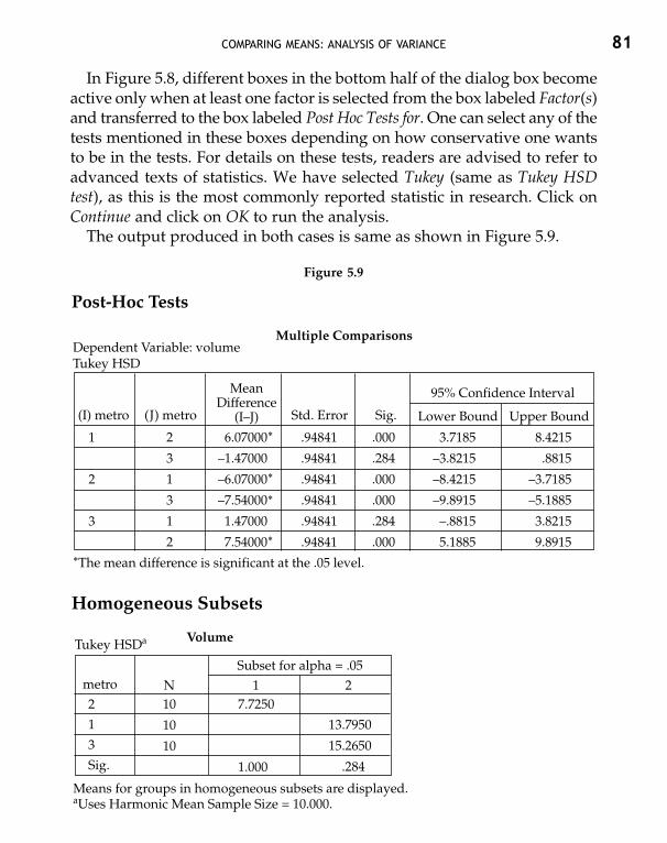
COMPARING MEANS: ANALYSIS OF VARIANCE 81
In Figure 5.8, different boxes in the bottom half of the dialog box becomeactive only when at least one factor is selected from the box labeled Factor(s)and transferred to the box labeled Post Hoc Tests for. One can select any of thetests mentioned in these boxes depending on how conservative one wantsto be in the tests. For details on these tests, readers are advised to refer toadvanced texts of statistics. We have selected Tukey (same as Tukey HSDtest), as this is the most commonly reported statistic in research. Click onContinue and click on OK to run the analysis.
The output produced in both cases is same as shown in Figure 5.9.
Figure 5.9

82 STATISTICAL METHODS FOR PRACTICE AND RESEARCH
The Post-Hoc test presents the result of the comparison between all thepossible pairs. Since we have three groups, a total of six pairs will be possiblein which three will be mirror images (1–2 and 2–1, 1–3 and 3–1, 2–3 and 3–2).The results are shown in three rows. The p-value for city 1- city 2 and city 2-city 3 comparison is shown as 0.000, whereas it is 0.284 for city 1- city 3 com-parison. This means that the average sales of gasoline between city 1 andcity 2 as well as city 2 and city 3 are significantly different, whereas the sameis not significantly different between city 1 and city 3.
The same result is also shown in another form in the table labeledHomogeneous Subsets. In this table, the groups are arranged in the increasingorder by the mean value. City 2 having the smallest mean value of gasolinesale is listed first followed by city 1 and city 3. On the right-hand side, thegroups are clubbed in homogenous subsets. City 2 with a mean of 7.725 isput under subset 1 and city 1 and 3 with means of 13.795 and 15.265 are putunder subset 2. This means that city 1 and 3 do not significantly differ fromeach other and form a homogeneous subset whereas they are different fromcity 2.
Performing Planned Comparisons
In this section, we will demonstrate planned comparisons for H02 and H03
of example 5.1. In the case of Univariate GLM, SPSS allows us to choosefrom a list of preset contrasts. However, in the case of One-Way ANOVA, thecontrasts have to be specified as will be explained later. First we explainthe specifying contrasts in Univariate GLM. Click on Contrasts in themain dialog box as shown in Figure 5.2. The resulting dialog box is shownin Figure 5.10.
Click on the drop down arrow opposite Contrasts in Figure 5.10 to view thelist of contrasts available. In this case, there are a total of six preset contrastsavailable: Deviation, Simple, Difference, Helmert, Repeated, and Polynomial. Ifyou select any of these and right click the mouse on it, SPSS Help will showthe description of the particular command. For example, we get thefollowing description on selecting Deviation and right clicking on it:
Compares the effect of each category of the predictor variable or factor, exceptone, to the overall effect. Select either First or Last as the omitted category.

COMPARING MEANS: ANALYSIS OF VARIANCE 83
Figure 5.10
In our example, by selecting Deviation, we can perform two comparisons.If we select metro 1 (first) to be omitted, then the average gasoline sale formetro 2 and 3 will be compared with the overall average (gasoline sale inmetro 1, 2 and 3 together). If we select metro 3 (first) to be omitted, then theaverage gasoline sale for metro 1 and 2 will be compared with the overallaverage. The other preset contrasts also have similar explanations.
In the case of One-Way ANOVA, clicking on Contrasts on the main dialogbox (Figure 5.1) opens a dialog box as shown in Figure 5.11. Earlier, in thesection on Multiple Comparisons, we explained that contrast coefficientsfor testing H02 and H03 are –1, 1, 0 and 2, –1, –1. To specify these coefficients,type them in the Coefficients box and click on the Add button. This will trans-fer the coefficients to the bigger box. The coefficients should be entered oneat a time with the coefficient of the lowest numbered group entering first.Click on Next to enter another set of coefficients. The phrase Contrast 1 of 1will get converted to Contrast 2 of 2 and the boxes will become empty.Enter 2, –1, and –1 for testing the second hypothesis. Steps for enteringthese two sets of coefficients are given below for clarity:
Enter –1 in the box labeled CoefficientsClick on the Add buttonEnter 1 in the box labeled CoefficientsClick on the Add button

84 STATISTICAL METHODS FOR PRACTICE AND RESEARCH
Enter 0 in the box labeled CoefficientsClick on the Add button
Coefficients for first contrast entered. Now click on the Next button.
Enter 2 in the box labeled CoefficientsClick on the Add buttonEnter –1 in the box labeled CoefficientsClick on the Add buttonEnter –1 in the box labeled CoefficientsClick on the Add button
This completes the process for entering both sets of contrast coefficients.Now click on Continue to return to the main dialog box and click on OK torun the analysis.
Figure 5.12 presents the specific part of the output related to contrasts.The output first shows the contrast coefficients assigned by us, followed bythe results of the significance test for each contrast. Two sets of results aregiven for each contrast, assuming variances to be equal and unequal. Theresult with the assumption of equal variances is the one more commonlyused as unequal variance violates the ANOVA assumption.
Figure 5.11

COMPARING MEANS: ANALYSIS OF VARIANCE 85
Figure 5.12
The first contrast tests if the average sale in metro 1 is the same as that inmetro 2. The test result shows that the t statistic is –6.400 with 27 degrees offreedom. The corresponding two-tailed p-value is less than 0.0005. Therefore,we can reject the null hypothesis and conclude that there is significant dif-ference in the average sale of gasoline in metro 1 and 2.
The second contrast tests if the average sale in metro 1 is same as themean of the average sale in metro 2 and 3. The test result shows that thet-statistic is 2.800 with 27 degrees of freedom. The corresponding two-tailedp-value is less than 0.009. Therefore, we can reject this null hypothesis also.
5.2.3 Two-Way Between-Groups ANOVA
In two-way analysis, we have two independent variables or factors and weare interested in knowing their effect on the same dependent variable. Thefollowing example illustrates how this analysis can be performed.
Example 5.2
An MBA aspirant was interested in knowing the impact of educational back-ground (arts/commerce and science/engineering) on the final placementsalaries. He is also aware that previous work experience has an impact onthe salaries. Therefore, he chooses educational background and work
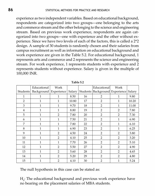
86 STATISTICAL METHODS FOR PRACTICE AND RESEARCH
experience as two independent variables. Based on educational background,respondents are categorized into two groups—one belonging to the artsand commerce stream and the other belonging to the science and engineeringstream. Based on previous work experience, respondents are again cat-egorized into two groups—one with experience and the other without ex-perience. Since we have two levels of each of the factors, this is called a 2*2design. A sample of 30 students is randomly chosen and their salaries fromcampus recruitment as well as information on educational background andwork experience are given in the Table 5.2. For educational background, 1represents arts and commerce and 2 represents the science and engineeringstream. For work experience, 1 represents students with experience and 2represents students without experience. Salary is given in the multiple of100,000 INR.
Table 5.2
Educational Work Educational WorkStudents Background Experience Salary Students Background Experience Salary
1 1 1 8.50 16 2 1 9.802 1 1 10.80 17 2 1 10.203 1 1 9.70 18 2 1 11.004 1 1 8.80 19 2 2 7.805 1 2 7.80 20 2 2 7.306 1 1 7.50 21 2 1 6.907 1 1 7.80 22 2 1 6.108 1 1 6.90 23 2 1 6.259 1 2 4.50 24 2 2 3.80
10 1 2 4.10 25 2 2 3.2011 1 1 7.70 26 2 2 5.1012 1 2 5.50 27 2 2 4.9013 1 2 5.60 28 2 2 4.6514 1 2 5.20 29 2 2 4.8015 1 2 4.10 30 2 1 5.24
The null hypothesis in this case can be stated as:
H0: The educational background and previous work experience haveno bearing on the placement salaries of MBA students.

COMPARING MEANS: ANALYSIS OF VARIANCE 87
The corresponding alternate hypothesis could be that the MBA studentsfrom science stream and/or with previous work experience will get moresalaries during final placements.
The variables are labeled as students, eduback, workexp, and salary. Clickon Analyze, which will produce a drop down menu, choose General LinearModel from that and click on Univariate. The resulting dialog box is shownin Figure 5.13.
Figure 5.13
Transfer the dependent variable (salary) into the Dependent variable boxand the independent or factor variables (eduback and workexp) into theFixed Factor(s) box. Click on Options to ask for additional statistics. The dialogbox obtained by clicking on Options is shown in Figure 5.14.
Select the variables for which you want descriptive statistics from theleft-hand side box labeled Factor(s) and Factor Interactions to the right-handside box labeled Display Means for. By selecting the interaction, one can getthe mean of the dependent variable for different combinations of theindependent variables. Click on Continue to return to the mail dialog boxand click on OK to run the analysis.

88 STATISTICAL METHODS FOR PRACTICE AND RESEARCH
Please note that selecting Post-Hoc tests will not produce any results inthis case as there are only two levels of each factor. A significant F-statisticitself tells that one group is significantly different from the other. Post-Hoctests are meaningful if there are more than two levels of at least one of theindependent variables.
Output for Two-Way ANOVA (Univariate GLM)
The output is shown in Figure 5.15. The first table labeled Between-SubjectsFactors gives the number of subjects in each level of the factor. In this case,we have 15 students belonging to each level of the two factors. The secondtable labeled Descriptive Statistics gives us the mean, standard deviation,and number of cases for the combination of different levels of the factors.
Figure 5.14

COMPARING MEANS: ANALYSIS OF VARIANCE 89
In this case, from the first row of the Descriptive Statistics table, we can findthat the mean salary of students with work experience and from arts orcommerce backgrounds is 8.46 lakh, i.e., Rs 846,000.
Figure 5.15
aR Squared = .487 (Adjusted R Squared = .428).

90 STATISTICAL METHODS FOR PRACTICE AND RESEARCH
The third table labeled Tests of Between-Subjects Effects gives the ANOVAresults. The explanation for various columns is same as given earlier incase of One-Way ANOVA.
We can see that the F-statistic corresponding to work experience is 23.896,which is significant at p < .001. F-statistic for educational background is0.243, which is insignificant as p = .626. The interaction between work experi-ence and educational background is also insignificant. Therefore the nullhypothesis (H0) is only partially supported. While the previous work experi-ence has a significant impact on the placement salaries of MBA students,their previous educational background does not.
The results will be reported as:
Previous work experience has a significant effect on the placement salariesof MBA students, F (1, 26) = 23.896, p < .001. However, previous educa-tion background does not affect the final placement salaries significantly,F (1, 26) = 0.243, p = .626. The interaction of previous work experience andeducational background also does not affect the placement salaries significantly,F (1, 26) = 0.151, p = .701.
SYNTAX
The syntax for obtaining the above output is given below:
UNIANOVAsalary BY workexp eduback/METHOD = SSTYPE(3)/INTERCEPT = INCLUDE/EMMEANS = TABLES(workexp)/EMMEANS = TABLES(eduback)/EMMEANS = TABLES(workexp∗eduback)/PRINT = DESCRIPTIVE ETASQ/CRITERIA = ALPHA(.05)/DESIGN = workexp eduback workexp∗eduback.

6
Chi-Square Test of Independence
for Discrete Data
Chi-square (χ2) is one of the very popular methods for testing hypotheseson discrete data. As explained in Chapter 1, on basic statistical concepts,discrete data can be nominal or ordinal. Finding descriptive statistics forsuch data is meaningless. The only summary statistics useful for such dataare frequencies and percentages. Contingency tables along with some chi-square statistics are used on such kind of data. Given below are some ex-amples of business and social sciences related studies where the chi-squaretest of independence can be used along with contingency tables to get ameaningful insight into the problem:
• An international business researcher wants to establish if the per-formance (categorized as loss, breakeven and profit) of a firm is de-pendent on which country (categorized as low, middle, and highincome) it is located in.
• An organizations’ researcher wants to determine if the satisfactionlevel (on a scale from 1 to 3) of the employees of a firm is dependenton their placement (local or international) within a firm.
• A social researcher wants to establish if the attitude towards pre-marital sex is dependent on the gender of the respondent.
6.1 BASIC CONCEPTS
There are three different types of chi-square analysis:
1. Chi-square test for goodness of fit.2. Chi-square test for homogeneity.3. Chi-square test of independence.

92 STATISTICAL METHODS FOR PRACTICE AND RESEARCH
The chi-square test for goodness of fit determines if the sample underinvestigation has been drawn from a population, which follows somespecified distribution, while the test for homogeneity investigates the issuewhether several populations are homogeneous with respect to a particularcharacteristic. These two are not very common methods employed inbusiness research and will not be dealt with here.
6.1.1 Chi-Square Test of Independence
The chi-square test of independence is used to test the hypothesis that twocategorical variables are independent of each other. A small chi-square stat-istic indicates that the null hypothesis is correct and that the two variablesare independent of each other.
The procedure involves comparing the observed cell frequencies withthe expected cell frequencies. Observed cell frequencies are the actualnumber of cases falling in different cells of the contingency table and ex-pected frequencies are the number of cases that should fall in each cell ifthere is no relationship between the two categorical variables. The basis ofthe test is difference between the observed frequency and the expected fre-quency of each cell of the contingency table. While observed cell frequenciescan be directly obtained from the given data, the expected cell frequenciesare calculated by multiplying the total of the row by the total of the columnto which the cell belongs and then dividing by the total sample size.
Along with the chi-square statistic, we also need to find the degrees offreedom associated with the contingency table to find the significance ofthe relationship. Degrees of freedom is calculated by multiplying the numberof rows minus one by the number of columns minus one. The degrees offreedom and significance level are used to find the values of chi-square fromthe standard tables. If the tabulated chi-square value is less than the calcu-lated chi-square value, the null hypothesis is rejected and we conclude thatthere is some significant association between the two variables.
The test can also be applied to ordinal categorical variables. While wecan test the independence of relationship between only two variables at atime, the variables themselves can have any number of levels.

CHI-SQUARE TEST OF INDEPENDENCE FOR DISCRETE DATA 93
6.1.2 Contingency Tables
It is often useful to look at contingency tables along with the results of thechi-square test to gain useful insight into the data. Contingency tablespresent the data in RXC tables where R is the number of rows and C is thenumber of columns. If the row variable has 3 categories and column variablehas 2 categories, then the contingency table produced will be a 3X2 table.The use of the contingency table has been elaborated in more detail throughthe example in this chapter.
6.2 USING SPSS
Solved Example
A researcher was interested in knowing whether the performance of firmsbelonging to the automobile sector is independent of the location of thefirm. She developed a measure of performance on a nominal scale from1 to 3–1 representing loss, 2 breakeven, and 3 profit. The location of thefirm was put in one of the two categories—1 representing low- and middle-income countries and 2 representing high-income countries. The data onthese two variables, collected for 45 corporations for a particular year ispresented in Table 6.1.
Table 6.1
Firm Location Performance Firm Location Performance Firm Location Performance1 1 1 16 1 3 31 2 22 1 1 17 1 3 32 2 23 1 1 18 1 3 33 2 24 1 1 19 1 3 34 2 25 1 1 20 1 3 35 2 26 1 1 21 1 3 36 2 27 1 2 22 1 3 37 2 38 1 2 23 1 3 38 2 39 1 2 24 2 1 39 2 3
10 1 2 25 2 1 40 2 311 1 2 26 2 1 41 2 312 1 3 27 2 1 42 2 313 1 3 28 2 1 43 2 314 1 3 29 2 2 44 2 315 1 3 30 2 2 45 2 3

94 STATISTICAL METHODS FOR PRACTICE AND RESEARCH
The null hypothesis in this case is that performance of the firm is inde-pendent of its location. In other words, there is no significant difference inthe performance of the firms located at different places.
The given data is entered in the data editor. Click on Analyze, which willproduce a drop down menu, choose Descriptive Statistics and then clickon Crosstabs as shown in Figure 6.1. The resulting dialog box is shown inFigure 6.2.
Figure 6.1
Select the variable you want to create the row of your contingency tableand transfer it to the box labeled Row(s), transfer the other variable to thebox labeled Column(s). By choosing which variable to transfer to these twoboxes, you may choose the way you want the contingency table to appear.In this example we transfer Location to the box labeled Row(s) and Performanceto the box labeled Column(s). Next, click on the Statistics button which bringsup a dialog box as shown in Figure 6.3.
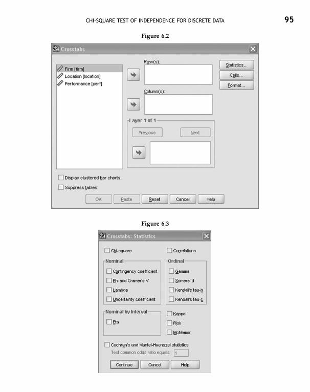
CHI-SQUARE TEST OF INDEPENDENCE FOR DISCRETE DATA 95
Figure 6.3
Figure 6.2

96 STATISTICAL METHODS FOR PRACTICE AND RESEARCH
Select the first box labeled Chi-square and click on the Continue button toreturn to the previous screen. Now click on the button labeled Cells whichbrings up a dialog box as shown in Figure 6.4.
Figure 6.4
Select the values you want to produce in your output. In this example wehave selected observed and expected counts. Readers may try other options.Click on Continue to return to the main dialog box (Figure 6.2). The buttonlabeled Format can be used to arrange the output in ascending or descendingorder. Click on OK to run the analysis.
Output
The output for Crosstabs is shown in Figure 6.5.
The first box labeled Case Processing Summary gives some details aboutthe cases in the data file. The second box labeled Location*PerformanceCrosstabulation gives the descriptive statistics requested in the analysis. In

CHI-SQUARE TEST OF INDEPENDENCE FOR DISCRETE DATA 97
this example, we requested for actual and expected count, which is producedfor each location (in rows) and each performance category (in columns).Count tells the actual frequency falling into a particular cell. Expected Countgives the expected frequency for each cell assuming no association. Thevalues on each row give information for each level of the column variable
Figure 6.5
a0 cells (.0%) have expected count less than 5. The minimum expected count is 5.38.

98 STATISTICAL METHODS FOR PRACTICE AND RESEARCH
whereas the values on each column give information about each level ofthe row variable. A chi-square test is not suitable if there are less than 5 casesin any of the cells.
The last box labeled Chi-Square Tests gives the results of the chi-square test.Several statistics are reported here but the one most commonly used is thePearson Chi-Square. We reject the null hypothesis if 2-sided significance re-ported in the last column and in the row corresponding to the Pearson Chi-Square is less than the significance level selected (5% or 10%).
In our example the p-value of .552 is much higher than the commonlyaccepted levels of either .05 or .10. So we cannot reject the null hypothesis.In other words, there is no significant relation between the performance ofa firm and its location. The result is reported as given below:
There was no significant relationship at 10% significance level betweenperformance of a firm and its location (χ2 = 1.190, df = 2, p = .552).
SYNTAX
The syntax for obtaining the above output is given below (loc and perf arethe variable names used for location and performance respectively):
CROSSTABS/TABLES=loc BY perf/FORMAT= AVALUE TABLES/STATISTIC=CHISQ/CELLS= COUNT EXPECTED.

7
Correlation Analysis
Correlation is a measure of relationship between two variables. It has wideapplication in business and statistics. Given below are some commonapplications of correlation analysis in business and social sciences:
• Marketing: The marketing manager wants to know if price reductionhas any impact on increasing sales.
• Production: The production department wants to know if the numberof defective items produced has anything to do with the age of themachine.
• Human Resource: The HR department wants to know if the productivityof its workers decreases with the number of hours they put in.
• Social Sciences: A social activist wants to know if increasing femaleliteracy has any impact in increasing the age of marriage of the girlchild.
• Research: An educationist wants to know if enforcing stricter attendancerules helps students in performing better in their studies.
7.1 BASIC CONCEPTS
7.1.1 Correlation Coefficient
The correlation coefficient gives a mathematical value for measuring thestrength of the linear relationship between two variables. It can take valuesfrom –1 to 1 with:
1. +1 representing absolute positive linear relationship (as X increases,Y increases).

100 STATISTICAL METHODS FOR PRACTICE AND RESEARCH
2. 0 representing no linear relationship (X and Y have no pattern).3. –1 representing absolute inverse relationship (as X increases,
Y decreases).
In the SPSS program, you have an option to choose from three types ofcorrelation coefficients: Pearson’s, Kendall’s tau-b, and Spearman’s. WhilePearson’s coefficient is commonly used for continuous data, the other twoare used mainly for ranked data.
7.1.2 Nature of Variables
Originally correlation analysis was conceptualized for use when the twovariables between which correlation is to be established are equal intervalor ratio scaled in their level of measurement, such as age, weight etc.Technically correlation analysis can be run with any kind of data, but theoutput will be of no use if a correlation is run on a categorical variable withmore than two categories. For example, in a data set, if the respondents arecategorized according to nationalities and religions, correlation betweenthese variables is meaningless.
7.1.3 Bivariate/Partial Correlation
Bivariate correlation tests the strength of the relationship between two vari-ables without giving any consideration to the interference some other variablemight cause to the relationship between the two variables being tested. Forexample, while testing the correlation between the academic perform-ance and attendance of a student, bivariate correlation will not consider theimpact of some other variables like motivation level or age. In such cases, abivariate analysis may show us a strong relationship between attendanceand academic performance; but in reality, this strong relationship could bethe result of some other extraneous factor like age or motivation level etc.In such cases a partial correlation should be used. It allows us to examine thecorrelation between two variables while controlling for the effects of one ormore of the additional variables without throwing out any of the data.
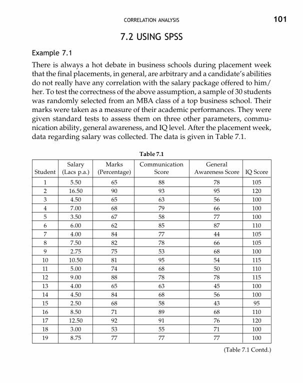
CORRELATION ANALYSIS 101
7.2 USING SPSS
Example 7.1
There is always a hot debate in business schools during placement weekthat the final placements, in general, are arbitrary and a candidate’s abilitiesdo not really have any correlation with the salary package offered to him/her. To test the correctness of the above assumption, a sample of 30 studentswas randomly selected from an MBA class of a top business school. Theirmarks were taken as a measure of their academic performances. They weregiven standard tests to assess them on three other parameters, commu-nication ability, general awareness, and IQ level. After the placement week,data regarding salary was collected. The data is given in Table 7.1.
Table 7.1
Salary Marks Communication GeneralStudent (Lacs p.a.) (Percentage) Score Awareness Score IQ Score
1 5.50 65 88 78 1052 16.50 90 93 95 1203 4.50 65 63 56 1004 7.00 68 79 66 1005 3.50 67 58 77 1006 6.00 62 85 87 1107 4.00 84 77 44 1058 7.50 82 78 66 1059 2.75 75 53 68 100
10 10.50 81 95 54 11511 5.00 74 68 50 11012 9.00 88 78 78 11513 4.00 65 63 45 10014 4.50 84 68 56 10015 2.50 68 58 43 9516 8.50 71 89 68 11017 12.50 92 91 76 12018 3.00 53 55 71 10019 8.75 77 77 77 100
(Table 7.1 Contd.)

102 STATISTICAL METHODS FOR PRACTICE AND RESEARCH
Salary Marks Communication GeneralStudent (Lacs p.a.) (Percentage) Score Awareness Score IQ Score
20 6.50 68 79 45 10521 13.50 89 89 56 11522 5.50 68 64 43 10023 4.00 63 62 40 10024 5.00 65 69 55 10025 7.60 74 71 68 105
Here we want to test the validity of the assumption that there is no correl-ation between the given variables. We also want to calculate the bivariateand partial correlation coefficients for the variables.
The data is entered in the data editor and the variables are labeled asstudent, salary, marks, communic, genawar, and iq respectively. Click on Analyze,which will produce a drop down menu as shown in Figure 7.1, choose Cor-relate. There are three types of correlation exercises shown under Correlate—Bivariate, Partial, and Distances. We will explain the computation procedurefor bivariate and partial correlation here.
Figure 7.1
(Table 7.1 Contd.)

CORRELATION ANALYSIS 103
7.2.1 Bivariate Correlation
To obtain bivariate correlations click on Bivariate as shown in Figure 7.1.The resulting dialog box is shown in Figure 7.2.
Choose the variables for which the correlation is to be studied from theleft-hand side box and move them to the right-hand side box labeled Vari-ables. Once any two variables are transferred to the variables box, theOK button becomes active. We will transfer all the variables other than StudentNo to the right-hand side box. There are some default selections at the bottomof the window; these can be changed by clicking on the appropriate boxes.For our purpose, we will use the most commonly used Pearson’s coefficient.
Next, while choosing between one-tailed and two-tailed test of signifi-cance, we have to see if we are making any directional prediction as ex-plained in Section 2.4.3 in Chapter 2. The one-tailed test is appropriate if weare making predictions about a positive or negative relationship betweenthe variables; however, the two-tailed test should be used if there is no pre-diction about the direction of relation between the variables to be tested.Finally Flag significant correlations asks SPSS to print an asterisk next to eachcorrelation that is significant at the 0.05 significance level and two asterisksnext to each correlation that is significant at the 0.01 significance level,
Figure 7.2

104 STATISTICAL METHODS FOR PRACTICE AND RESEARCH
so that the output can be read easily. The default selections will serve thepurpose for the problem at hand. We may choose means and standard devi-ations from the Options button if we wish to compute these figures for thegiven data. After making appropriate selections, click on OK to run theanalysis.
Output
The output produced is shown in Figure 7.3. The output gives correlationsfor all the pairs of variables and each correlation is produced twice in thematrix. We get the following 10 correlations for the given example:
1. Salary and academic performance (marks)2. Salary and communication abilities3. Salary and general awareness4. Salary and IQ level5. Academic performance (marks) and communication abilities6. Academic performance (marks) and general awareness
Figure 7.3
∗Correlation is significant at the 0.05 level (2-tailed).∗∗Correlation is significant at the 0.01 level (2-tailed).

CORRELATION ANALYSIS 105
7. Academic performance (marks) and IQ level8. Communication abilities and general awareness9. Communication abilities and IQ level
10. General awareness and IQ level
In each cell of the correlation matrix, we get Pearson’s correlationcoefficient, p-value for two-tailed test of significance, and the sample size.From the output, we can see that the correlation coefficient between salaryand marks is 0.702 and the p-value for two-tailed test of significance is lessthan 0.0005 (values less than 0.0005 are shown as 0.000 in SPSS outputs).From these figures we can conclude that there is a strong positive correlationbetween Salary and Marks and that this correlation is significant at thesignificance level of 0.01. Results for correlations between other set ofvariables can also be interpreted similarly. We can see that General AwarenessScore and Marks are not significantly correlated (r = 0.204, p = 0.328). Allother variables are significantly correlated with each other.
SYNTAX
The syntax for obtaining the above output is given below:
CORRELATIONS/VARIABLES=salary marks comunic genawar iq/PRINT=TWOTAIL NOSIG/MISSING=PAIRWISE.
7.2.2 Partial Correlation
To obtain partial correlations, click on Partial as shown in Figure 7.1. Theresulting dialog box is shown in Figure 7.4.
In partial correlation, we are interested in knowing the extent of thespecific relationship between two variables, factoring out the effect of oneor more other variables. For the given example, we want to find the cor-relation between salary and marks while controlling for the effect of theIQ level. We will transfer Salary and Marks to the Variables box and IQ Scoreto the Controlling for box. The resulting dialog box is shown in Figure 7.5.Now click on OK to run the analysis.

106 STATISTICAL METHODS FOR PRACTICE AND RESEARCH
Figure 7.4
Figure 7.5

CORRELATION ANALYSIS 107
Output
The output produced is shown in Figure 7.6. The variable we are controllingfor in the analysis (for example, IQ in our case) is shown in the left-handside. We can see that the correlation coefficient is not just considerablysmaller (0.333 as compared to 0.702 in case of bivariate), but the p-value isalso much higher (0.112 as compared to less than 0.005 in case of bivariate).This means that if we control for the IQ level of the students, the salarieswill not be significantly related to the academic performance of the students,which is good news indeed for happy-go-lucky students!
Figure 7.6
SYNTAX
The syntax for obtaining the above output is given below:
PARTIAL CORR/VARIABLES= salary marks BY iq/SIGNIFICANCE=TWOTAIL/MISSING=LISTWISE.

8
Multiple Regression
Regression analysis is used to assess the relationship between one dependentvariable (DV) and several independent variables (IVs). This is the mostcommonly used technique in much of the social sciences research. Givenbelow are some common applications of regression analysis in businessand social sciences:
• Marketing: The marketing manager wants to know if sales is dependenton factors such as advertising spend, number of products introduced,number of sales personnel etc.
• Human Resource: The HR department wants to predict the efficiencyof management trainees based on their academic performance, leader-ship abilities, IQ level etc.
• Social Sciences: A social researcher wants to predict the age of marriageof a girl based on characteristics such as her education level, parent’seducation level, number of siblings, and parent’s annual income.
8.1 BASIC CONCEPTS
8.1.1 Regression Coefficient
Regression coefficient is a measure of how strongly each IV (also knownas predictor variable) predicts the DV. There are two types of regressioncoefficients—unstandardized coefficients and standardized coefficients, alsoknown as beta value. The unstandardized coefficients can be used in theequation as coefficients of different IVs along with the constant term to pre-dict the value of DV. The standardized coefficient (beta) is, however, measuredin standard deviations. A beta value of 2 associated with a particular IV

MULTIPLE REGRESSION 109
indicates that a change of 1 standard deviation in that particular IV willresult in a change of 2 standard deviations in the DV.
If there is just one IV to predict one DV, the beta value obtained would besame as the correlation coefficient between the DV and the IV.
8.1.2 R Values
R represents the correlation between the observed values and the predictedvalues (based on the regression equation obtained) of the DV. R Square isthe square of R and gives the proportion of variance in the dependent vari-able accounted for by the set of IVs chosen for the model. R Square is usedto find out how well the IVs are able to predict the DV. However, theR Square value tends to be a bit inflated when the number of IVs is more orwhen the number of cases is large. The adjusted R Square takes into accountthese things and gives more accurate information about the fitness of themodel. For example, an adjusted R Square value of 0.70 would mean thatthe IVs in the model can predict 70% of the variance in the DV. While innatural science research it is not uncommon to get R Square values as highas 0.99, a much lower value (0.10–0.20) of R Square is acceptable in socialscience research.
8.1.3 Design Issues
There are a number of design issues in regression analysis and readers aresuggested to consult a standard statistics textbook for details. We discusshere two important aspects of design issues—Ratio of cases to IVs and Multi-collinearity.
Case to IVs ratio should be substantial for a meaningful regression solu-tion. The rule of the thumb is to have the sample size at least as much as50 + 8n for testing the multiple correlation and 104 + n for testing individualpredictors, where n is the number of IVs.
Multicollinearity refers to a situation when two or more IVs are highlycorrelated with each other. Multicollinearity causes an inflation in the stand-ard error of regression coefficients resulting in a reduction of their signifi-cance. Care should be taken in choosing the IVs such that they are not highly

110 STATISTICAL METHODS FOR PRACTICE AND RESEARCH
correlated with each other. SPSS gives diagnostic statistics for multicol-linearity which are explained later in this chapter.
8.1.4 Multiple Regression Types
There are three major types of multiple regression: standard multiple re-gression, hierarchical or sequential regression and stepwise or statisticalregression.
In standard multiple regression, all the IVs are entered into the equationtogether. In hierarchical regression, IVs are entered in a pre-specified mannerby the researcher, which is driven by theoretical considerations. In stepwiseregression, order of entry of variable is solely based on statistical criteria.This is, however, a controversial procedure and hardly used in social scienceresearch.
8.2 USING SPSS
Example 8.1
A researcher wants to test some hypotheses regarding the relationship be-tween size and age of a firm and its performance in a particular industry.Size was measured by the number of employees (in 100s) working in thefirm, age was the number of years for which the firm has been operating,and performance was measured by return on equity. A sample of 50 firmswas selected at random. Data on these variables is given in Table 8.1.
Table 8.1
Firm ID Performance Size Age Firm ID Performance Size Age
1 10.24 20 40 26 0.86 19 432 3.84 2 41 27 32.92 4 503 10.45 20 43 28 4.01 8 444 27.42 19 25 29 24.10 6 355 14.80 3 29 30 13.93 9 246 11.42 33 7 31 2.48 65 297 1.90 4 30 32 8.27 4 438 23.51 29 57 33 2.65 8 41
(Table 8.1 Contd.)

MULTIPLE REGRESSION 111
Firm ID Performance Size Age Firm ID Performance Size Age
9 15.52 87 15 34 13.48 7 4810 6.40 29 48 35 3.30 28 1811 –2.53 11 44 36 6.44 15 3212 5.77 20 34 37 –3.89 9 3213 –4.35 17 16 38 1.26 78 1414 2.81 8 18 39 24.48 99 1215 24.70 13 16 40 14.40 8 1516 11.92 66 17 41 0.76 6 1917 –18.75 8 40 42 2.29 1 2118 50.32 85 16 43 26.91 4 8619 –16.83 1 44 44 24.64 1 5620 15.31 5 34 45 20.62 51 2121 5.51 7 22 46 6.72 1 2222 6.06 61 31 47 13.80 7 6123 14.81 21 16 48 23.91 5 8824 42.42 93 12 49 1.88 1 1125 –3.18 2 17 50 1.79 66 25
The researcher wanted to test the following two hypotheses:
H1: Performance of a firm is positively related to its size.H2: Performance of a firm is positively related to its age.
The null hypotheses in this case would be that performance is not relatedto the size or age of the firm.
8.2.1 Standard Multiple Regression
The given data is entered in the data editor and the variables are labeled asid, perf, size, and age. Click on Analyze, which will produce a drop down menu,choose Regression from that and click on Linear as shown in Figure 8.1. Theresulting dialog box is shown in Figure 8.2.
Transfer the dependent variable into the right-hand side box labeled De-pendent. Transfer the independent variables into the box labeled Independent(s).The DV in our example is Performance and the IVs are size and age. Next, we
(Table 8.1 Contd.)

112 STATISTICAL METHODS FOR PRACTICE AND RESEARCH
Figure 8.1
Figure 8.2

MULTIPLE REGRESSION 113
have to select the method for analysis in the box labeled Method. SPSS givesfive options here: Enter, Stepwise, Remove, Backward, and Forward. In theabsence of a strong theoretical reason for using a particular method, Entershould be used. The box labeled Selection Variable is used if we want torestrict the analysis to cases satisfying particular selection criteria. The boxlabeled Case Labels is used for designating a variable to identify points onplots.
After making the appropriate selections click on the Statistics button. Thiswill produce a dialog box labeled Linear Regression: Statistics as shown inFigure 8.3.
Figure 8.3
Tick against the statistics you want in the output. The Estimates optiongives the estimate of regression coefficients.The Model fit option gives thefit indices for the overall model. The Descriptives option gives the descriptivestatistics of the selected variables. The Collinearity diagnostics option producesimportant statistics used for assessing the presence of multicollinearity inthe data. These four are selected in our example. Besides these, the R squared

114 STATISTICAL METHODS FOR PRACTICE AND RESEARCH
change option is used to get the incremental R Square value when the modelschange. It should be selected in the case of hierarchical regression or whenwe use any other method in place of Enter for regression strategy. Othersare not commonly used. Click on the Continue button to return to the maindialog box.
There are some other buttons in the main dialog box for advanced users.The Plots button in the main dialog box (Figure 8.2) may be used forproducing histograms and normal probability plots of residuals. TheSave button can be used to save statistics like predicted values, residuals,and distances. The Options button can be used to specify the criteria for step-wise regression. Advanced users may experiment with these additionalfeatures.
Click on OK in the main dialog box (Figure 8.2) to run the analysis.
Output
The output produced has several tables titled Descriptive Statistics, Cor-relations, Variables Entered/Removed, Model Summary, ANOVA, Coefficients,Collinearity Diagnostics. Descriptive Statistics, Correlations, and ANOVA tablesare explained earlier in the book. The remaining tables are explained in thefollowing paragraphs.
Figure 8.4 has two tables titled Variables Entered/Removed and Model Sum-mary. The table titled Variables Entered/Removed tells us about the independentvariables and the regression method used. Here we can see that both theIVs, Age and Size are entered simultaneously for the analysis as we selectedthe Enter method. The next table titled Model Summary gives us the R valuesfor assessing the overall fit of the model. The adjusted R Square value inthis case is 0.138. This tells us that the two IVs in our model account for13.8% variance in the DV—performance of the firms. Clearly this is not avery good model as there are factors other than age and size of a firm whichshould also be used to predict a firm’s performance. What value of R Squareis good enough to claim that a model is good, is a judgement call of the re-searcher and varies for different research streams. One should look at articlesin commonly used journals in one’s stream to find out the acceptable R Squarevalue for a ‘good’ model fit.

MULTIPLE REGRESSION 115
Figure 8.5 has tables titled Coefficients and Collinearity Diagnostics.
Figure 8.5
Figure 8.4

116 STATISTICAL METHODS FOR PRACTICE AND RESEARCH
The first of these tables gives the regression coefficients and their sig-nificance. These regression coefficients can be used to construct an OrdinaryLeast Squares (OLS) equation and also to test the hypotheses on each of theIVs. Using the regression coefficients for IVs and the constant term givenunder the column labeled B, one can construct the OLS equation for pre-dicting firm performance as:
Performance = –0.356 + (0.209) (Size) + (0.190) (Age)
The values given under the column labeled Beta can also be used to con-struct the regression equation if all IVs were first converted to Z scores.A variable can be converted to Z score by first subtracting the mean of thevariable and then dividing the resultant value by standard deviation for aparticular variable and in a particular sample. This process is known asstandardization of variables. If all variables are in standardized form the Yintercept (constant term) will always be zero. This is why we do not get aconstant term under the Beta column. The OLS equation in this case will be:
ZPerformance = (0.447) (ZSize) + (0.257) (ZAge)
Now we test our hypotheses. The null hypothesis is that there is no rela-tionship, i.e., the beta coefficient is not different from zero. The p-value forbeta coefficient of Size is 0.003, the same for Age is 0.083. Both these valuesare significant at 10% significance level. Thus we cannot accept the nullhypothesis. In other words, we can claim that the performance of a firm ispositively related to its size and age. Please note that at 5% significancelevel, the relationship between performance and age will not be significant.
The last column in the Coefficients table is Collinearity Statistics. In thiscolumn and in the last table titled Collinearity Diagnostics, we get statisticsfor testing multicollinearity in the model. Collinearity Statistics gives twovalues—Tolerance and VIF (variance inflation factor). As one can see Toleranceis just the inverse of VIF. A value of VIF higher than five (or Tolerance lessthan 0.2) indicates the presence of multicollinearity. In social sciences re-search, a VIF value as high as 10 is considered to be acceptable. The ConditionIndex obtained in the table titled Collinearity Diagnostics is another measure

MULTIPLE REGRESSION 117
of multicollinearity. The rule of thumb in this case is that there is multi-collinearity if any two IVs have Variance Proportions in excess of 0.9 (columnvalues) corresponding to any row in which Condition Index is in excess of 30.Although these diagnostic statistics are commonly used to detect multi-collinearity, there effectiveness is controversial and one should be carefulabout their use.
Once multicollinearity is detected in the model, the regression coefficientsare likely to be meaningless. One may consider removing some IVs whichare highly correlated to reduce multicollinearity. However, if theoreticalconsiderations do not allow removing any of the IVs, one may consideranother type of regression called ridge regression. Ridge regression is a con-troversial process and not available in SPSS through the point and clickmethod. If, after consulting literature, one still wants to use it, it is availablethrough a macro in SPSS.
SYNTAX
The syntax for obtaining the above output is given below:
REGRESSION/DESCRIPTIVES MEAN STDDEV CORR SIG N/MISSING LISTWISE/STATISTICS COEFF OUTS R ANOVA COLLIN TOL/CRITERIA=PIN(.05) POUT(.10)/NOORIGIN/DEPENDENT perf/METHOD=ENTER size age.
8.2.2 Hierarchical Regression
Hierarchical regression is in many ways similar to a standard multiple re-gression, the only difference being in the way IVs are entered in the model.For example, in the above solved example, theoretical considerations maydemand that we first assess the model with only the size of the firm andintroduce the age of the firm in the second stage. This modeling procedureis called hierarchical, as we are entering the IVs based on certain rules of

118 STATISTICAL METHODS FOR PRACTICE AND RESEARCH
hierarchy. Researchers commonly use this method when they have atheoretical reason to build models in a hierarchical manner. The procedureis explained briefly for the solved example for standard multiple regression.
Follow the steps as in the case of standard multiple regression and openthe dialog box as shown in Figure 8.2. Transfer Performance into the boxlabeled Dependent and size into the box labeled Independent(s). Once size isentered, a button labeled Next becomes active above this box. Clicking onNext will again empty the box labeled Independent(s). Transfer the secondIV, age into this box. Next, click on the Statistics button to open the dialogbox shown in Figure 8.3. Select R Squared change in this box since we areinterested in finding the incremental R square when we include more IVs.Click on OK to run the analysis.
Output
The output produced is quite similar to the one we got in standard multipleregression. The relevant output is shown in Figures 8.6 and 8.7.
Figure 8.6
The first table labeled titled Entered/Removed shows that size was enteredin Model 1 followed by age in Model 2. Please note that Model 1 includesonly size as IV whereas Model 2 includes both size as well as age as IVs.

MULTIPLE REGRESSION 119
The next table—Model Summary in the same figure—shows differentR values along with change statistics for both models in different rows.In this table we get some additional statistics under the column ChangeStatistics. Under Change Statistics, the first column labeled R Square Changegives change in the value of R Square between the models. The last columnlabeled Sig. F Change tests whether there is a significant improvement inmodels as we introduce additional IVs. In other words it tells us if the in-clusion of additional IVs in different steps helps in explaining significantadditional variance in the DV. We can see that the R Square Change value in
Figure 8.7

120 STATISTICAL METHODS FOR PRACTICE AND RESEARCH
row two is 0.055. This means that inclusion of age after size helps in explain-ing the additional 5.5% variance in the performance of the firms. Beforeinclusion of age, size accounted for 11.8 variance (R Squared value) in per-formance. Please note that R Square Change is same as the difference in theR Square values between Model 2 and Model 1. The p-value for testingsignificance of corresponding F change is 0.083, significant at 10% levelof significance. This means that inclusion of age significantly improves ourmodel to predict firm performance.
Let us take a look at Figure 8.7 now. The first table labeled Coefficients givesregression coefficients and related statistics for two models separately indifferent rows. The second table labeled Excluded Variables lists the variablesthat are not included in earlier models but included in later models. This isnot of much practical importance. Explanations for rest of the items in thisfigure are similar to what has been given under standard multiple regression.
SYNTAX
The syntax for obtaining the above output is given below:
REGRESSION/DESCRIPTIVES MEAN STDDEV CORR SIG N/MISSING LISTWISE/STATISTICS COEFF OUTS R ANOVA COLLIN TOL CHANGE/CRITERIA=PIN(.05) POUT(.10)/NOORIGIN/DEPENDENT perf/METHOD=ENTER size/METHOD=ENTER age.

9
Logistic Regression
Logistic regression is used to predict a discrete outcome based on variableswhich may be discrete, continuous, or mixed. Thus when the dependentvariable may have two or more than two discrete outcomes, logistic regres-sion is a commonly used technique. Following are some common appli-cations of logistic regression analysis in business and social sciences:
• Marketing: An international marketing manager of a big firm is inter-ested in predicting whether foreign subsidiaries in a particular countrywill make profits or losses or will they just breakeven depending onthe characteristics of the host country of the subsidiary’s operations.The DV here is clearly discrete with three possible outcomes—loss,breakeven, or profit.
• Human Resource: The HR manager of a company wants to predict theabsenteeism pattern of its employees based on their individual char-acteristics. The DV here is dichotomous—absent or present.
• Social Sciences: A psychologist wants to predict the pattern of awakeningfrom sleep at night based on the personal characteristics of the subjectsand characteristics of the ambience. The DV is again dichotomous.
9.1 BASIC CONCEPTS
9.1.1 Logistic Regression Coefficients
Logistic regression computes the log odds for a particular outcome. Theodds of an outcome are given by the ratio of the probability of it happeningand not happening as P/(1–P), where P is the probability of an event. There
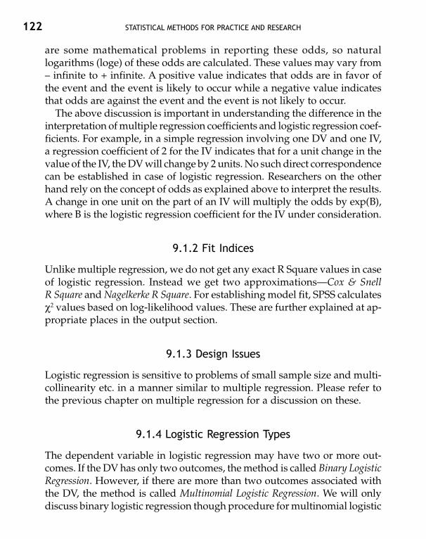
122 STATISTICAL METHODS FOR PRACTICE AND RESEARCH
are some mathematical problems in reporting these odds, so naturallogarithms (loge) of these odds are calculated. These values may vary from– infinite to + infinite. A positive value indicates that odds are in favor ofthe event and the event is likely to occur while a negative value indicatesthat odds are against the event and the event is not likely to occur.
The above discussion is important in understanding the difference in theinterpretation of multiple regression coefficients and logistic regression coef-ficients. For example, in a simple regression involving one DV and one IV,a regression coefficient of 2 for the IV indicates that for a unit change in thevalue of the IV, the DV will change by 2 units. No such direct correspondencecan be established in case of logistic regression. Researchers on the otherhand rely on the concept of odds as explained above to interpret the results.A change in one unit on the part of an IV will multiply the odds by exp(B),where B is the logistic regression coefficient for the IV under consideration.
9.1.2 Fit Indices
Unlike multiple regression, we do not get any exact R Square values in caseof logistic regression. Instead we get two approximations—Cox & SnellR Square and Nagelkerke R Square. For establishing model fit, SPSS calculatesχ2 values based on log-likelihood values. These are further explained at ap-propriate places in the output section.
9.1.3 Design Issues
Logistic regression is sensitive to problems of small sample size and multi-collinearity etc. in a manner similar to multiple regression. Please refer tothe previous chapter on multiple regression for a discussion on these.
9.1.4 Logistic Regression Types
The dependent variable in logistic regression may have two or more out-comes. If the DV has only two outcomes, the method is called Binary LogisticRegression. However, if there are more than two outcomes associated withthe DV, the method is called Multinomial Logistic Regression. We will onlydiscuss binary logistic regression though procedure for multinomial logistic

LOGISTIC REGRESSION 123
regression is pretty much the same. Like multiple regression, the model de-velopment can be in the standard manner or hierarchical manner.
In the following section we explain the hierarchical binary logistic re-gression procedure. Please note that building the model in a hierarchicalmanner should be driven by sound theoretical considerations. The hierarchyof variables specified in this example is only for illustrative purpose.
9.2 USING SPSS
Example 9.1
As in example 8.1 in the multiple regression chapter, suppose that a re-searcher wants to test the same hypotheses regarding the relationship be-tween size and age of a firm and its performance in a particular industry.Size is measured by the number of employees (in 100s) working in the firm,age is the number of years for which the firm has been operating. The per-formance variable is, however, measured with the help of a survey in whichthe CEO of the firm has to mention if his firm is making profit or loss. Aresponse of 1 indicates profit and 0 indicates loss. A sample of 50 firms isselected at random. Data on these variables is given in Table 9.1.
Table 9.1
Firm ID Performance Size Age Firm ID Performance Size Age
1 1 20 40 26 1 19 432 0 2 41 27 1 4 503 1 20 43 28 0 8 444 1 19 25 29 0 6 355 0 3 29 30 0 9 246 0 33 7 31 1 65 297 0 4 30 32 0 4 438 1 29 57 33 0 8 419 1 87 15 34 0 7 48
10 1 29 48 35 1 28 1811 0 11 44 36 1 15 3212 1 20 34 37 0 9 3213 0 17 16 38 1 78 14
(Table 9.1 Contd.)

124 STATISTICAL METHODS FOR PRACTICE AND RESEARCH
Firm ID Performance Size Age Firm ID Performance Size Age
14 0 8 18 39 1 99 1215 0 13 16 40 0 8 1516 1 66 17 41 0 6 1917 1 8 40 42 0 1 2118 1 85 16 43 1 4 8619 0 1 44 44 1 1 5620 0 5 34 45 1 51 2121 0 7 22 46 0 1 2222 1 61 31 47 1 7 6123 1 21 16 48 1 5 8824 1 93 12 49 0 1 1125 0 2 17 50 1 66 25
The researcher wants to test following two hypotheses:
H1: Performance of a firm is positively related to its size.H2: Performance of a firm is positively related to its age.
The null hypotheses in this case would be that performance is not relatedto the size or age of the firm. In addition to the above, the researcher alsowants to test for the interaction effect of age and size on firm performance.The interaction hypothesis is given below:
H3: Size of a firm interacts with its age in determining firm performancesuch that effect of size on performance increases with the age of thefirms. In other words, bigger and older firms have better performancethan bigger but newer firms.
While calculating hierarchical regressions, the researcher has to decidethe hierarchy of the variables entering into the equation which should betheory driven. In this example, we are also testing an interaction hypothesis(H3). When testing for interaction effects, it is advisable to build modelssuch that we enter all the main effects in one model first and then enterinteraction effects in another model. Thus the hierarchy of variables in ourexample will be to enter the main effects of size and age in Model 1 andenter the interaction effect of size and age in Model 2.
(Table 9.1 Contd.)

LOGISTIC REGRESSION 125
Figure 9.1
Figure 9.2
The given data is entered in the data editor and the variables are labeledas id, perf, size, and age. Click on Analyze, which will produce a drop downmenu, choose Regression from that and click on Binary Logistic as shown inFigure 9.1. The resulting dialog box is shown in Figure 9.2.

126 STATISTICAL METHODS FOR PRACTICE AND RESEARCH
Transfer the DV (Performance) into the right-hand side box labeledDependent. Transfer the IVs into the box labeled Covariates. Size and age aretwo IVs here. On transferring any one IV into the Covariates box, the buttonlabeled Next becomes active. After size and age are transferred, click on theNext button. Now we have to enter the interaction effect in the second model.Select size and age simultaneously. Once any two variables are selectedsimultaneously, a button labeled >a∗b> becomes active. Click on this andthe two variables will appear as age∗size in the covariates box. This essentiallymeans that we are entering a multiplication term for age and size.
Next we have to select the method for analysis in the box labeled Method.SPSS gives seven options, of which Enter is most commonly used. Once theDV and IVs are transferred to the relevant boxes, the button labeledCategorical becomes active. If any of the IVs are categorical, click on this anddefine the categorical variables. In this example, we do not have any cat-egorical IVs. For common purpose one does not need to use the Save andOptions buttons. Advanced users may experiment with these. Click on OKto run the analysis.
Output
The output is shown in Figures 9.3 to 9.5. In Figure 9.3, the first table titledCase Processing Summary gives the description of cases selected for analysis.The second table titled Dependent Variable Encoding describes how the twooutcomes of performance (loss and profit) have been coded.
We get some more tables under the heading Block 0: Beginning Block. Weare not showing these tables here. These are not of much relevance andshould be ignored. Next, we get output under the heading Block 1: Method =Enter as shown in Figure 9.4. The first table titled Omnibus Tests of ModelCoefficients gives general tests of how well the model performs. In the nexttable labeled Model Summary we get –2 Log likelihood and two other statisticswhich are equivalent to R Square values in multiple regression. –2 Log likeli-hood is used to compare models and assess if the inclusion of additionalterms in the model significantly improves model fit or not. Cox & Snell andNagelkerke R Square values give an approximation about how much vari-ance in the dependent variable can be explained with the hypothesizedmodel. In this example age and size can explain between 6.04% and 8.05%variance in the firm’s performance.

LOGISTIC REGRESSION 127
Next, we get the classification table, which summarizes the results of ourprediction about firm performance based on size and age of a firm. We cansee that our model can correctly predict 83.3% of the loss making firms and84.6% of the profit making firms. Over all, our model predicts 84% of thefirms correctly.
The last table gives Beta coefficients for the independent variables alongwith their significance. Positive Beta coefficients for size and age mean thatwith increasing size and age of a firm, its chances of having a profitableperformance improve. In the column under Sig. we can see that size is sig-nificant at 0.005 level and age is significant at 0.01 level.
The Beta coefficients in logistic regression are not easily interpretable.For their interpretation we look at the last column under Exp(B). Exp(B)takes a value of more than one if Beta coefficient is positive and less than 1
Figure 9.3
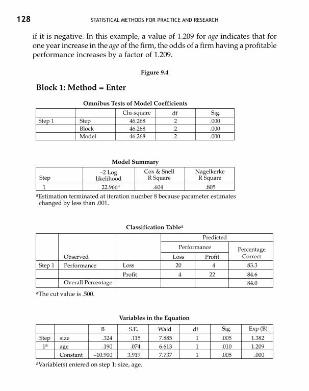
128 STATISTICAL METHODS FOR PRACTICE AND RESEARCH
if it is negative. In this example, a value of 1.209 for age indicates that forone year increase in the age of the firm, the odds of a firm having a profitableperformance increases by a factor of 1.209.
Figure 9.4
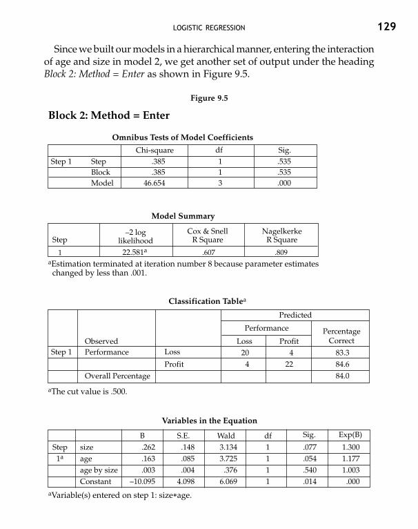
LOGISTIC REGRESSION 129
Since we built our models in a hierarchical manner, entering the interactionof age and size in model 2, we get another set of output under the headingBlock 2: Method = Enter as shown in Figure 9.5.
Figure 9.5

130 STATISTICAL METHODS FOR PRACTICE AND RESEARCH
Looking at the last table labeled Variables in the Equation in Figure 9.5, wecan see that the coefficient of Age by Size is not significant (p = 0.54). This isalso evident from the first table labeled Omnibus Tests of Model Coefficientsin Figure 9.5. The incremental chi-square value is shown as 0.385 and notsignificant (p = 0.535), implying that the inclusion of an additional term inthe form of interaction between Age and Size does not improve the model fit.
SYNTAX
The syntax for obtaining the above output is given below:
LOGISTIC REGRESSION VAR=perf/METHOD=ENTER size age/METHOD=ENTER age∗size/CRITERIA PIN(.05) POUT(.10) ITERATE(20) CUT(.5).

10
Data Reduction and Scale Reliability:
Factor Analysis
Factor analysis (FA) and Principal Components Analysis (PCA) are techniquesused when the researcher is interested in identifying a smaller number offactors underlying a large number of observed variables. Variables that havea high correlation between them and are largely independent of other subsetsof variables, are combined into factors. A common usage of PCA and FA isin developing objective instruments for measuring constructs which arenot directly observable in real life. The examples given below demonstratethe usage of factor analysis:
• A researcher is interested in identifying celebrity characteristics whichare perceived by the general public to be important. The researchermay choose a variety of variables such as intelligence, attractiveness,dependability etc. and ask the respondents to rate their importancefor a celebrity. A factor analysis of these items may reveal the under-lying dimensions of important celebrity characteristics.
• A researcher collects data on many variables representing a few under-lying dimensions. She then wants to have a score for each of thesedimensions, which can be further used for regression or other analysis.One can obtain such scores for each of the dimension by performing afactor analysis.
10.1 BASIC CONCEPTS
10.1.1 Factor and Component
Factors are produced by FA, while components are produced by PCA. BothFA and PCA essentially are data reduction techniques. Mathematically, the

132 STATISTICAL METHODS FOR PRACTICE AND RESEARCH
difference is in the variance of the observed variables that is analyzed. InPCA, all the variance in the observed variables is analyzed whereas in FA,only shared variance is analyzed. Even though PCA is different from othertechniques of FA, at many places it is treated as one of the FA techniques.For this reason, we will use the word components and factors inter-changeably in this chapter.
10.1.2 Exploratory and Confirmatory Factor Analysis
As the name suggests, in exploratory FA (EFA) we are interested in exploringthe underlying dimensions that could have caused correlations among theobserved variables. In case of confirmatory FA (CFA), the researcher is inter-ested in testing whether the correlations among the observed variables areconsistent with the hypothesized factor structure. Thus while EFA dealswith theory building, CFA deals with theory testing. The term FA generallymeans exploratory FA. SPSS can only do EFA analysis. For CFA, one has touse other programs such as AMOS, LISEREL, EQS etc.
10.1.3 Extraction
Extraction refers to the process of obtaining underlying factors or com-ponents. Besides PCA, SPSS offers several other extraction methods suchas principal axis factoring (PAF), alpha factoring etc. The differences areprimarily mathematical in nature and generate similar results in most ofthe cases. The two most commonly used extraction methods are PCA andPAF. If the researcher has designed the study based on a theoretical con-sideration, PFA should be the preferred choice. However, if the main aim ofthe researcher is simply to reduce the number of variables, PCA is a betterchoice.
10.1.4 Factor Loadings
FA produces factor loadings for each combination of extracted factors andthe observed variables. Factor loadings are similar to correlation coefficientsbetween the factors and the variables. Thus higher the factor loading, themore likely it is that the factor underlies that variable. Factor loadings helpin identifying which variables are associated with the particular factors.

DATA REDUCTION AND SCALE RELIABILITY 133
10.1.5 Rotation
Factor loadings obtained from extraction may not present a clear picture ofthe factor structure of the data set. After extraction, while we may be able toidentify the number of factors, we may not know the exact way in whichthe observed variables load on different factors. Unrotated factor loadingsare extremely hard to interpret, regardless of the extraction methods. Rotationhelps in arriving at a simple pattern of factor loadings by maximizing highcorrelations and minimizing low ones.
Rotation could be orthogonal or oblique. Orthogonal rotation should beused under the assumption that the underlying factors are uncorrelatedwith each other. However, if the researcher has theoretical reasons to believethat the factors may be correlated, oblique rotation is a better choice. SPSSoffers three orthogonal rotation techniques—varimax, quartimax, andequamax; and two oblique rotation techniques—direct oblimin and promax.Of these, varimax is the most commonly used rotation technique.
10.1.6 Communalities
Communality gives the variance accounted for a particular variable by allthe factors. Mathematically, it is the sum of squared loadings for a variableacross all the factors. The higher the value of communality for a particularvariable after extraction, higher is its amount of variance explained by theextracted factors.
10.1.7 Eigenvalue and Scree Plot
Both eigenvalue and scree plot are used to decide the number of under-lying factors after extraction. Eigenvalue is the measure of amount of totalvariance in the data explained by a factor. Factor analysis initially considersthe number of factors to be same as the total number of variables. Look-ing at the eigenvalue, one can determine if the factor explains sufficientamount of variance to be considered as a meaningful factor. An eigenvalueof less than 1 essentially means that the factor explains less variance than asingle variable, and therefore should not be considered to be a meaningfulfactor.

134 STATISTICAL METHODS FOR PRACTICE AND RESEARCH
Scree plot is a graphical presentation of eigenvalues of all of the factorsinitially considered for extraction. Usage of scree plot for deciding on thenumber of factors is explained later with an example.
10.1.8 Scale Reliability
After identifying the dimensions underlying a factor, a researcher may pre-pare a scale of those dimensions to measure the factor. Such a scale has tobe tested for validity and reliability. Proper validity and reliability testingcan be done using CFA. However, researchers commonly use the Cronbachalpha coefficient for establishing scale reliability. The Cronbach alphacoefficient is an indicator of internal consistency of the scale. A high value ofthe Cronbach alpha coefficient suggests that the items that make up the scale“hang together” and measure the same underlying construct. A value ofCronbach alpha above 0.70 can be used as a reasonable test of scale reliability.
10.1.9 Sample Size Considerations
An adequate sample size is important for identifying the correct factor struc-ture. A sample size of less than 100 is not very suitable for conducting factoranalysis. A sample size above 500 is considered to be excellent. As a rule ofthumb, a sample size of 200–300 should be considered to be adequate for aproper analysis.
10.2 USING SPSS
10.2.1 Factor Analysis
Example 10.1
An advertising firm was interested in developing a scale to measure thecredibility of celebrities in public opinion so that the right celebrities couldbe chosen for endorsing products. Based on extensive literature, theyidentified a list of 14 qualities, which could be important for establishingthe credibility of a celebrity in public opinion. Respondents were asked torank the credibility of some popular celebrities on a scale of 1 to 5 withrespect to these qualities. The data for 56 respondents are given at the end

DATA REDUCTION AND SCALE RELIABILITY 135
of this chapter in Table 10.1. Please note that 56 is too small a sample size; how-ever, it will serve our purpose of demonstrating the analysis. The 15 itemsmeasured the following characteristics:
Attractive, classy, beautiful, elegant, sexy, dependable, honest, reliable, trust-worthy, sincere, skilled, expert, experienced, knowledgeable, qualified.
The given data was entered in the data editor and the items were assignednames and labels. The procedure for using the SPSS program in developingthis scale is as follows: click on Analyze, which will produce a drop downmenu, choose Data reduction from the menu and click on Factor as shown inFigure 10.1. The resulting dialog box is shown in Figure 10.2.
Figure 10.1

136 STATISTICAL METHODS FOR PRACTICE AND RESEARCH
Figure 10.2
Select the variables from the left-hand side box and transfer them to thebox labeled Variables. On the right-hand of the box, there are five buttons.The first one labeled Descriptives gives you the option to choose variousdescriptive statistics. You can leave it at its default setting, which will giveyou the initial solution of FA. The other four buttons are important tounderstand the proper usage of FA. Click on the button labeled Extractionwhich brings up a dialog box as shown in Figure 10.3.
Figure 10.3

DATA REDUCTION AND SCALE RELIABILITY 137
There are many extraction methods listed, which can be obtained byclicking on the drop down arrow in the box against Method. Two commonlyused extraction methods are Principal Components and Principal AxisFactoring. As discussed earlier, Principal Components is a data reduction tech-nique and not strictly an FA technique. However, since the same is given inmost of the programs as one of the extraction technique, people often confuseit with FA. Typically, if there is no mention of an extraction method in FA,one should assume that Principal Axis Factoring has been used. We haveselected Principal Axis Factoring in this case. Next, we have to select whetherwe want to analyze the correlation matrix or the covariance matrix for FA.The recommended option for beginners is to use the correlation matrix, ad-vanced users may, however, choose the covariance matrix for special cases.Click against Unrotated factor solution and Scree plot to display the two in theoutput. At the bottom of this box, we can specify the number of factors wewant to extract. Default setting is to choose factors with eigenvalues greaterthan 1 as factors with eigenvalues less than 1 do not carry enough infor-mation. We can also specify the number of factors if we have a specific re-quirement to extract a certain number of factors. This is not advisable though,as the analysis in this case becomes purely mathematical. Click on Continueto return to the main dialog box. Next, click on the button labeled Rotation,to specify the specific rotation strategy you want to adopt. This brings up adialog box as shown in Figure 10.4.
Figure 10.4

138 STATISTICAL METHODS FOR PRACTICE AND RESEARCH
The SPSS program gives five options for rotations. Select Varimax fromthis box and click against Rotated solution. Readers are encouraged to tryother rotation methods. In most of the cases, there is not much difference inthe factor solutions obtained from different rotation methods. Click onContinue to return to the main dialog box.
Next, click on the button labeled Scores. From the resulting dialog box asshown in Figure 10.5, we can choose to save scores for each factor in ourdata set. These scores get saved for each observation as a new variable,which can be used for regression analysis as a composite measure of under-lying dimensions. We did not choose to do so in our example as it is notrelated to our understanding of the FA technique and its output.
Figure 10.5
Finally click on the button labeled Options, which will bring up a dialogbox as shown in Figure 10.6. Here we can choose options for treating caseswith missing values and formatting the output. The choice of missing valuesshould always be the first one (Exclude cases listwise) unless one has anyspecific approach to deal with missing values. For a better display of theoutput, it is often useful to select the two options listed at the bottom of thisbox. The first option sorts the factor loadings by size and lists variables inthe same order. The second option hides factor loadings below the valuespecified by the researcher. It is advisable to suppress values below 0.40 asthis is a standard criterion used by researchers to identify important factorloadings. We have not done this in order to present the full output. Readersare advised to try running the analysis after suppressing values and comparethe ease of reading the two outputs. Click on Continue to return to the maindialog box and click on OK to run the analysis.

DATA REDUCTION AND SCALE RELIABILITY 139
Figure 10.6
Output
SPSS displays FA output in many tables depending on what we specifywhile selecting various options. These results are shown in Figures 10.7 to10.12. The first table titled Communalities (Figure 10.7) gives the initial andextraction communalities.
Figure 10.7
140 STATISTICAL METHODS FOR PRACTICE AND RESEARCH
The extraction communalities are useful as these are obtained using theextracted factors. Extraction communalities for a variable give the total amountof variance in that variable, explained by all the factors. In our example,90.84% of the variance in beautiful is explained by the extracted factors. If aparticular variable has low communality, it means that the extracted factorsare not able to explain much variance in that variable. Such variables maybe dropped from the analysis.
The next table titled Total Variance Explained (Figure 10.8) summarizes thetotal variance explained by the FA solution and gives an indication aboutthe number of useful factors. This table has three parts. The first part, titledInitial Eigenvalues gives the variance explained by all the possible factors.There are a total of 15 factors, which is same as the number of variablesentered into the FA. However, please note that these factors are not thesame as the variables. The first column under Initial Eigenvalues gives theeigenvalues for all the possible factors in a decreasing order. This is followedby the variance as a percentage of all the variance and cumulative variance.By simple computation, one can verify that the total variance explained isequal to the total number of factors (or variables), 14 in this case; and thepercentage of variance for the first factor will be same as its eigenvaluedivided by total variance.
The second part, titled Extraction Sums of Squared Loadings gives infor-mation for factors with eigenvalues greater than 1. The word “extraction”here refers to the fact that these values are calculated after factor extraction.In case of principal component analysis, these will be the same as initialeigenvalues. The figure under the column Cumulative % in this part indicatesthat the three extracted factors explain 64.87% of the variance.
The last part titled, Rotated Sums of Squared Loadings gives the informationfor extracted factors after rotation. Please note that after rotation, only therelative value of eigenvalues has changed, the cumulative percentage re-mains the same.
There are only three factors with eigenvalues greater than 1 suggesting athree-factor solution. Sometimes we may find eigenvalues of some of thefactors dropping below 1 after rotation. A judgement has to be made in suchcases about the number of factors to be extracted.
The scree plot shown in Figure 10.9 is another way of identifying thenumber of useful factors. We look for a sharp break in sizes of eigenvalues

Figu
re 1
0.8
Ext
ract
ion
Met
hod
: Pri
ncip
al A
xis
Fact
orin
g.

142 STATISTICAL METHODS FOR PRACTICE AND RESEARCH
which results in a change in the slope of the plot from steep to shallow. Wecan see that the slope of the scree plot changes from steep to shallow afterthe first three factors. The eigenvalue also drops from above 2 to less than 1when we move from factor 3 to factor 4. This suggests that a three-factorsolution may be the right choice.
Figure 10.9
The next table titled Factor Matrix (Figure 10.10) gives the factor loadingsbefore rotation is carried out. For each of the variables, we get a loading ineach of the columns representing factors. The variables are listed in thedecreasing order of factor loadings as we requested the same in the Optionswindow. The extraction communalities presented in the second column ofFigure 10.7 is a summation of the square of loadings on all the factors for aparticular variable. For example, the extraction communality value forHonest in Figure 10.7 can be obtained as:
(0.878)2 + (–0.071)2 + (–0.368)2 = 0.91
The factor loadings in the factor matrix are not easily interpretable. Wecan see that the variable Experienced has high loadings of 0.527 and 0.558 ontwo factors. Likewise, there are many other variables with high loadings

DATA REDUCTION AND SCALE RELIABILITY 143
on more than one factor in the factor matrix. Rotation sometimes solvesthis problem. Figure 10.11 presents the table titled Rotated Factor Matrix whichhas rotated loadings. For a good factor solution, a particular variable shouldload high on one factor and low on all other factors in the rotated factormatrix. Researchers commonly use a cut-off of 0.40 to identify high loadings.In this example, we can see that the variables which are loading high onfactor 1 have low loadings on factors 2 and 3. Likewise, those loading highon other factors have low loadings on the remaining factors. This is close tobeing an ideal situation. In case we find a variable loading high on morethan one factor, we may want to drop it from the analyses and make revisionsbased on theoretical considerations.
Once we obtain the variables corresponding to particular factors, we maygive suitable names to the factors. For example, in this case factor 1 comprisesfive variables—Honest, Trustworthy, Reliable, Sincere, and Dependable; factor 2
Figure 10.10
Factor Matrixa
Extraction Method: Principal Axis Factoring.a3 factors extracted. 15 iterations required.

144 STATISTICAL METHODS FOR PRACTICE AND RESEARCH
comprises four variables—Knowledgeable, Qualified, Experienced, and Expert;factor 3 comprises five variables—Beautiful, Attractive, Classy, Elegant, andSexy. These three factors can be clubbed together and termed Trust-worthiness, Expertise, and Attractiveness.
The last table titled Factor Transformation Matrix is only for the purpose ofproviding information. This matrix is used for carrying out the rotation. Itis of no use for the interpretation of results.
Figure 10.11
Rotated Factor Matrixa
Extraction Method: Principal Axis Factoring.Rotation Method: Varimax with Kaiser Normalization.aRotation converged in 5 iterations.

DATA REDUCTION AND SCALE RELIABILITY 145
Figure 10.12
Extraction Method: Principal Axis Factoring.Rotation Method: Varimax with Kaiser Normalization.
If we perform the principal component analysis in the place of principalaxis factoring, we will see the word “Component” in the place of “Factor”in the output.
SYNTAX
The syntax for obtaining the above output is given below:
FACTOR/VARIABLES attracti classy beautifu elegent sexy dependab honest reliabletrustwor sincere expert experien knowledg qualifie/MISSING LISTWISE/ANALYSIS attracti classy beautifu elegent sexy dependabhonest reliable trustwor sincere expert experien knowledg qualifie/PRINT INITIAL EXTRACTION ROTATION/FORMAT SORT BLANK(.40)/PLOT EIGEN/CRITERIA MINEIGEN(1) ITERATE(25)/EXTRACTION PAF/CRITERIA ITERATE(25)/ROTATION VARIMAX/METHOD=CORRELATION.
10.2.2 Scale Reliability
In the factor analysis example, we found three factors which we termed asTrustworthiness, Expertise, and Attractiveness. It will be premature to claimthat the underlying items of these factors make up the scale for measuring

146 STATISTICAL METHODS FOR PRACTICE AND RESEARCH
Figure 10.13
Figure 10.14
these factors. But for the purpose of illustration, we will assume this to becorrect. Now we want to measure the reliability of these scales.
Open the data file for Example 10.1. Click on Analyze, which will producea drop down menu, choose Scale from that and click on Reliability Analysis asshown in Figure 10.13. The resulting dialog box is shown in Figure 10.14.

DATA REDUCTION AND SCALE RELIABILITY 147
We can test the reliability of only one scale at a time. We illustrate herethe reliability testing for the scale on Trustworthiness. Select the items usedto measure Trustworthiness and transfer them to the box labeled Items. TheTrustworthiness scale items include dependable, honest, reliable, trustworthy,and sincere. Click on the button labeled Statistics which will open a dialogbox as shown in Figure 10.15.
Select the descriptive statistics for Item, Scale, and Scale if item deleted.Click on Continue to return to the main dialog box and click on OK to runthe analysis.
Figure 10.15
Output
The output is shown in Figures 10.16 and 10.17. In Figure 10.16, the first tabletitled Case Processing Summary gives the description of cases selected foranalysis. The second table titled Reliability Statistics gives the value of theCronbach alpha coefficient and the number of items selected for the scale.For our scale of Trustworthiness, we find the Cronbach alpha value to be 0.96.

148 STATISTICAL METHODS FOR PRACTICE AND RESEARCH
Figure 10.16
We also get the descriptive statistics as shown in Figure 10.17. The firsttable titled Item Statistics gives item-wise mean and standard deviationvalues. The second table titled Item-Total Statistics is important. The fourthcolumn in this table, titled Corrected Item-Total Correlation gives an indicationof the degree to which each item correlates with the composite score for thescale. The last column labeled Cronbach’s Alpha if Item Deleted gives the im-pact of removing each item on the alpha coefficient. Looking at these values,along with the Cronbach alpha coefficient values, one may decide to removesome of the items from the scale.

DATA REDUCTION AND SCALE RELIABILITY 149
Figure 10.17
SYNTAX
The syntax for obtaining the above output is given below:
RELIABILITY/VARIABLES=dependab honest reliable trustwor sincere/FORMAT=NOLABELS/SCALE(ALPHA)=ALL/MODEL=ALPHA/STATISTICS=DESCRIPTIVE SCALE/SUMMARY=TOTAL.

Tab
le 1
0.1
Tab
le 1
0.1
Dat
a fo
r E
xam
ple
10.
1
14
45
55
54
43
44
32
2
25
55
55
34
33
33
35
3
35
35
45
33
33
33
33
3
44
54
54
44
44
44
24
3
55
55
54
32
22
24
44
5
65
55
55
22
22
22
24
2
75
24
45
12
11
14
14
4
85
55
55
44
44
44
33
3
95
45
45
33
33
32
22
2
105
55
55
55
42
24
35
4
115
35
45
33
33
33
33
3
125
55
35
33
33
34
43
3
135
45
44
22
22
34
43
3
145
55
55
44
44
44
33
3
155
44
43
32
11
33
12
3
164
44
54
44
44
44
44
4
174
34
43
54
34
54
33
5
184
43
21
55
55
54
44
4
194
44
43
44
44
43
33
4
204
44
55
44
44
44
43
3
214
44
34
22
22
23
33
3
225
55
53
55
55
55
35
5
235
55
54
43
33
34
34
4
245
45
44
33
33
34
33
4
255
55
55
33
33
34
45
4
Tab
le 1
0.1
Dat
a fo
r E
xam
ple
10.
1Id
attractive
classy
beautiful
elegant
sexy
dependable
honest
reliable
trustworthy
sincere
expert
experienced
knowledgeable
qualified

265
54
44
44
44
44
34
3
275
55
53
55
55
55
35
5
285
45
44
33
33
34
44
4
295
55
55
33
22
25
22
2
305
55
43
33
32
34
22
2
315
45
44
23
33
31
11
1
325
44
44
33
34
44
43
3
334
35
35
33
54
34
45
4
345
55
55
44
44
44
44
4
355
55
55
55
55
55
55
5
364
44
44
44
44
44
44
4
375
45
55
33
33
23
12
2
385
35
35
33
33
44
44
3
395
55
55
43
23
43
44
5
404
34
44
32
11
13
14
1
414
44
54
44
44
44
44
4
425
55
55
55
55
55
44
5
434
34
35
21
21
22
34
4
445
45
45
44
44
43
44
4
455
55
53
33
33
44
34
3
465
55
44
22
22
22
55
5
475
55
55
55
55
55
55
5
485
45
45
33
33
33
33
3
495
45
45
55
45
44
43
4
505
55
55
33
34
41
11
1
514
55
55
44
44
44
44
4
524
44
34
22
22
23
33
3
535
55
53
33
33
44
34
3
544
55
45
23
23
33
34
4
555
45
45
33
33
33
45
5
564
24
53
22
22
22
22
2

152 STATISTICAL METHODS FOR PRACTICE AND RESEARCH
11
Advanced Data Handling in SPSS
In case of research based on secondary data, the number of cases may bequite large. Even in the case of survey and experimental research, it is notuncommon to have a few hundred cases. Researchers may need to runanalyses on a subset of the cases or create new variables from the existingvariables based on certain conditions. The commands described in thischapter are very useful for managing large and complex data files.
We use the data file of Example 3.1 given in Chapter 3 for illustration. Wediscuss the following data handling techniques in this chapter:
1. Sorting cases2. Merging files3. Aggregating cases4. Splitting files5. Selecting cases6. Recoding7. Computing new variables
All the commands used in this chapter are given under Data or Transformmenus.
11.1 SORTING CASES
Normally, the order of responses does not matter while running an analysis.Still, sometimes we may be interested in having the data in a particular orderin the editor window. This can be achieved by sorting files. In Example 3.1,if we want to see the responses in increasing order of respondents’ age anddecreasing order of sales, we can do this in the following manner.

ADVANCED DATA HANDLING IN SPSS 153
Click on Data in the data editor window and select Sort Cases from thedrop down menu as shown in Figure 11.1. This produces a dialog box asshown in Figure 11.2. The ascending or descending order has to be chosenbefore transferring a variable into the Sort by box. Since we want the data tobe in ascending order of age and descending order of sales, click on Ascendingand transfer age into the box labeled Sort by. Next, click on Descending andtransfer sales to the Sort by box. You may choose any number of variables tosort the data file. Click on OK and the data file will be sorted in the ascendingorder of age and descending order of sales.
Figure 11.1
SYNTAX
The syntax for performing the above discussed sort command is givenbelow:
SORT CASES BYage (A) sales (D).

154 STATISTICAL METHODS FOR PRACTICE AND RESEARCH
11.2 MERGING FILES
The merging of files becomes important when we have to add some casesto our data file or add some new variables. While coding data, it is a commonpractice that more than one coder does the data entry on a standard format.For example, if there is a two page questionnaire, one coder may be enteringdata for one page and the other coder may be entering for the other page.The only common thing the coders enter in this case is the identificationnumber (executiv in this case) of the respondents. Once we have these twofiles, we may want to merge them and create one file with all the variables.Likewise, it is possible that two coders enter the responses of half of therespondents each. In this case, we may want to merge cases from the twofiles into one file. We will illustrate the procedure only for merging variables.Cases can also be merged in a similar manner.
Before we explain the merging of files, we have to create two files whichhave to be merged. Save the data in Example 3.1 in an SPSS file with the filename “descriptives1”. In this file, keep only the gender, age, and region in-formation for each respondent. Create another file with the file name “des-criptives2” and keep the sales data for each respondent in this file. Pleasenote that both these files will have the executiv variable, which is nothingbut a unique identifier for each respondent. It is this identifier variable, basedon which the SPSS program will merge variables from the two files.
Before merging the two files, data in both the files should be sorted inascending order by the “By” variable, which is the key variable used for
Figure 11.2

ADVANCED DATA HANDLING IN SPSS 155
merging the files. In this example, executiv is the “By” variable. Sort both thefiles by executiv as explained in the previous section and save the files. Nowopen the file into which you want to merge the variables—descriptives1 inthis case.
Click on Data, choose Merge Files from the drop down menu and click onAdd Variables as shown in Figure 11.3. This produces a dialog box (Figure 11.4).This dialog box prompts you to select a data set from which you want tomerge the variables of interest. The data set could be an already open dataset or some external SPSS file. The dialog box shown in Figure 11.4 does notcome in earlier versions of SPSS, as one could not open multiple data editorwindows. Clicking on Browse in the second option will take you to the folderin which you have stored the file into which you are merging the variables(descriptives1). You have to select the second file (descriptives2) from whichyou want to merge variables. In case the second file is not stored in thesame folder as the first one, browse through folders as is done while openingany file and select the file. Once you select the second file, click Continueand a new dialog box will open as shown in Figure 11.5.
Figure 11.3

156 STATISTICAL METHODS FOR PRACTICE AND RESEARCH
Figure 11.4
Figure 11.5

ADVANCED DATA HANDLING IN SPSS 157
The left-hand side box labeled Excluded Variables lists the commonvariables in the two files. The right-hand side box labeled New Active Datasetlists the variables from both the files. To differentiate the variables from thetwo files, it puts ∗ against the variables from the file into which we aremerging the data and + against the variables which come from the externalfile. In this case, sales is the variable from the external file. If we do not wantcertain variables in the new file, we may discard them by selecting thevariables from the right-hand side box and transferring them into the Ex-cluded Variables box on the left-hand side.
Next, we have to specify the key variable by which we are matching thetwo files. In this case it is executiv. Select the key variable (executiv) and tickin the box against Match cases on key variables in sorted files. This activates thethree sub-options below it. Select the External file is keyed table and transferthe executiv into the box labeled Key Variables. This will essentially askSPSS to match sales values from the second file by the respondent’s ids. Wemay specify more than one key variable. Click on OK, and you will see awarning that the matching will fail if the data is not sorted in an ascendingorder. Click on OK again to complete the merging. You can check the datafile to see that the variable sales is added in the descriptives1 file.
SYNTAX
The syntax for performing the merging in the given example follows:
MATCH FILES /FILE=∗/TABLE=’E:\AAA\india\SPSS\data files\descriptives 2.sav’/BY executiv.EXECUTE.
The second row here specifies the file from which data is to be merged.
11.3 AGGREGATING CASES
The aggregate command may not be very useful for small data files, but be-comes essential while working with large files. By running an Aggregatecommand, we create a new data file with the variables specified by us. Theillustration given in this section will make this point clear.

158 STATISTICAL METHODS FOR PRACTICE AND RESEARCH
Supposing in Example 3.1, we are only interested in region-wise salesvalues. Click on Data in the data editor window and select Aggregate fromthe drop down menu as shown in Figure 11.1. This produces a dialog box asshown in Figure 11.6.
Figure 11.6
We have to specify the variables by which we want to aggregate our datain the Break Variable(s) box. In our example, since we want the data to be ag-gregated by regions, select and transfer region into the Break Variable(s) box.Next, we have to specify the variables which we want to aggregate into thebox labeled Summaries of Variable(s). Select sales and transfer it into this box.Once the summary variables are transferred, two additional buttons becomeactive below this box. Click on the button labeled Function which opens adialog box (Figure 11.7). We can specify the way we want to aggregatethe data from this box. The default setting is for mean, which will give you

ADVANCED DATA HANDLING IN SPSS 159
the mean of the sales value for all the regions. One can also choose to producesome specific values such as minimum, maximum etc. We let the defaultsetting stay as it is and click on Continue to return to the main dialog box(Figure 11.6).
Figure 11.7
Next, we can specify whether we want to add the aggregated variablesto the current data file, create a new data set with only the aggregated vari-ables or store the aggregated variables in a new file. We select to store thedata into a new file. This will save the aggregated data into a file named“aggr.sav” in the same location as the current working file. These settingscan be changed. If you open the aggregated file, you will see three rowscorresponding to three regions and two variables as shown in Figure 11.8.

160 STATISTICAL METHODS FOR PRACTICE AND RESEARCH
Figure 11.8
SYNTAX
The syntax for aggregating the variables is:
AGGREGATE/OUTFILE=’E:\AAA\india\SPSS\data files/aggr.sav’/BREAK=region/sales_mean_1 = MEAN(sales).
The second row specifies the location and name of the aggregated file tobe saved as a new file.
11.4 SPLITTING FILES
The Split File command temporarily splits the file into groups. All the ana-lyses done after splitting a file will be done separately on the different sub-groups and the output will be arranged according to these groups. Forexample, if we are interested in obtaining descriptive statistics about ageand sales by gender, we can split the file by the gender variable.
Click on Data in the data editor window and select Split File from thedrop down menu as shown in Figure 11.1. This produces a dialog box asshown in Figure 11.9.

ADVANCED DATA HANDLING IN SPSS 161
Figure 11.9
The default option in this window is to analyze all the cases. Select Comparegroups or Organize output by groups. The first option presents the output withinone section, comparing the groups, while the second option presents theoutput in different sections. Selecting either of these will activate the boxlabeled Groups Based on. Select gender and transfer to this box. Click on OKto complete splitting the file. Now if you run any analysis, two outputs willbe produced, one for males and the other for females.
Splitting file is a temporary option and you can cancel it by selectingAnalyze all cases, do not create groups.
SYNTAX
The syntax for splitting file by gender is given below:
SORT CASES BY gender.SPLIT FILESEPARATE BY gender.

162 STATISTICAL METHODS FOR PRACTICE AND RESEARCH
11.5 SELECTING CASES
We can run our analyses in a sub-sample of the total cases by specifying ourselection criteria using the Select Cases command. This is different from split-ting file as in the case of splitting a file, we get output by all the subgroupsspecified by a particular variable. In the split command, we cannot specifymultiple selection criteria. In addition, splitting a file by a continuous variableis meaningless.
Suppose we want to select a sub-sample of cases in which the age of the re-spondents is at least 22 years or above. Click on Data in the data editor windowand select Select Cases from the drop down menu as shown in Figure 11.1.This produces a dialog box (Figure 11.10).
Figure 11.10
The default setting is to run the analyses for all the cases. Tick against Ifcondition is satisfied, this will activate the button labeled If below it. Click on

ADVANCED DATA HANDLING IN SPSS 163
If, which opens a dialog box as shown in Figure 11.11. In this dialog box, wehave to specify the selection criteria. Since we want respondents with atleast 22 years of age, our selection criterion will be: age> = 22. Select age andtransfer it to the right-hand side box and specify this selection criterionusing the options given at the bottom of this box. We can also type multipleselection criteria in this box. For example, if we want to select a respondentover 27 years or below 25 years and belonging to region 1, we can specifythe following formula:
(age>27 or age<25) and region = 1
Figure 11.11
Click on Continue to return to the main dialog box (Figure 11.10). We canalso specify whether we want to filter out the unselected cases from analyses,copy selected cases to a new data set, or delete the unselected cases from thefile. It is advisable not to delete the cases as you may need the unselectedcases for future analyses. We choose the first option to filter out the un-selected cases. Click on OK to complete the selection. The data editor windowlooks as shown in Figure 11.12. SPSS puts a cross line through the casenumber which is not selected. One can revert to analyzing all the cases byselecting All cases from the main dialog box (Figure 11.10).

164 STATISTICAL METHODS FOR PRACTICE AND RESEARCH
Figure 11.12
SYNTAX
The syntax for specifying the above selection criteria is given below:
USE ALL.COMPUTE filter_$=(age>27 or age<25 and region=1).VARIABLE LABEL filter_$ ‘age>27 or age<25 and region=1 (FILTER)’.VALUE LABELS filter_$ 0 ‘Not Selected’ 1 ‘Selected’.FORMAT filter_$ (f1.0).FILTER BY filter_$.EXECUTE.
11.6 RECODING VALUES
Many times, we may want to recode some of the variables. This could bebecause we may obtain data in different format from surveys or secondaryresources and we may have to put them in a certain format for the purposeof analyses. For example, we may want to create two categories of re-spondents in the first example—one with age less than or equal to 25 years

ADVANCED DATA HANDLING IN SPSS 165
and the other with age greater than 25. We may also want to recode somevalues to missing values. The illustration below describes these options.
Click on Transform in the data editor window and select Recode intoDifferent Variables…from the drop down menu as shown in Figure 11.13.The SPSS program gives three options to recode. Recode into Same Variables…option replaces the current values with the recoded values. Recode intoDifferent Variables…option creates a new variable. Automatic Recode changescurrent values based on a pre-specified template. It is advisable to alwaysrecode into a new variable so that we can avoid the loss of original data incase of a wrong recode command. If a variable is recoded into the samevariable and the new file saved, there is no way we can get back the originalvariable. Click on Recode into Different Variables…which produces a dialogbox as shown in Figure 11.14.
Figure 11.13
Select age and transfer it into the box labeled Input Variable → OutputVariable. Once this is done, two boxes on the left-hand side become active.We have to specify the name and label of the new variable in these boxes.Type age_cat in the box labeled Name and Age Category as its label in the boxlabeled Label. Now click on the button labeled Change to transfer the nameof the output variable into the box labeled Input variable → Output variable.The resulting dialog box appears as shown in Figure 11.15.

166 STATISTICAL METHODS FOR PRACTICE AND RESEARCH
Next, click on the box labeled Old and New Values which produces a dialogbox as shown in Figure 11.16. In this box, we have to specify our recodingstrategy which is to recode age less than or equal to 25 as a zero, and morethan 25 as one.
Figure 11.14
Figure 11.15

ADVANCED DATA HANDLING IN SPSS 167
Figure 11.16
To specify the first range, tick against Range, LOWEST through value andspecify 25 in the box opposite to it. Next, specify zero in the right-hand sidebox against Value. Click on Add to transfer these values to the box labeledOld -> New. In a similar manner specify the second range in the box Range,value through HIGHEST, specify 1 as the value for this range in the Value boxand click on Add. The resulting dialog box appears as shown in Figure 11.17.Click on Continue to return to the main dialog box (Figure 11.15).
We can further specify some selection criteria for running the recode com-mand on a sub-sample of cases. This can be done by clicking on the buttonlabeled If as explained in the previous section. Click on OK to complete therecoding exercise. A new variable named age_cat is created in the data file,which takes a value of 0 for age less than or equal to 25 years and 1 for agegreater than 25 years.
SYNTAX
The syntax for the recoding is given below:
RECODEage(Lowest thru 25=0) (26 thru Highest=1) INTO age_cat .VARIABLE LABELS age_cat ‘Age Category’.EXECUTE.

168 STATISTICAL METHODS FOR PRACTICE AND RESEARCH
11.7 COMPUTING NEW VARIABLES
Quite often we need to create many new variables from the original variableson which we collect the data. A very common usage is to create an interactionterm while performing moderated regression analysis. Suppose we wantto create an interaction between age and gender.
Click on Transform in the data editor window and select Compute Variables…from the drop down menu as shown in Figure 11.13. This produces a dialogbox (Figure 11.18). Specify the name of the variable to be created in theTarget Variable box and specify the numerical expression in the box labeledNumeric Expression. We can indicate the type and label of the variable byclicking on the button labeled Type & Label. We can either type the ex-pressions or select the variables and use appropriate buttons to specify theexpression. For creating an interaction term between age and gender, wecreate the following expression:
gen_age = gender∗age
The selection criteria can also be specified at the bottom of box. Click onOK to complete the computation of the new variable. In the data file, a newvariable named gen_age is created.
Figure 11.17
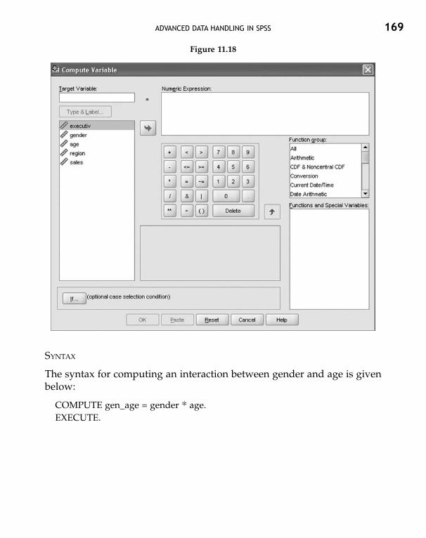
ADVANCED DATA HANDLING IN SPSS 169
Figure 11.18
SYNTAX
The syntax for computing an interaction between gender and age is givenbelow:
COMPUTE gen_age = gender ∗ age.EXECUTE.

Bibliography
Aiken, L. S. and West, S. G. (1991). Multiple Regression: Testing and Interpreting Interactions.Newbury Park, CA: Sage Publications.
Aneshensel, C. S. (2002). Theory-Based Data Analysis for the Social Sciences. Thousand Oaks,CA: Sage Publications.
Baron, R. M. and Kenny, D. A. (1986). “The Moderator-Mediator Variable Distinction inSocial Psychological Research: Conceptual, Strategic, and Statistical Considerations”,Journal of Personality and Social Psychology, 51: 1173–82.
Kline, P. (1994). An Easy Guide to Factor Analysis. London: Routledge.MacCallum, R. C., Widaman, K. F., Zhang, S. and Hong, S. (1999). “Sample Size in Factor
Analysis”, Psychological Methods, 4: 84–99.Pedhazur, E. J. (1997). Multiple Regression in Behavior Research, 3rd Edition. Orlando FL:
Harcourt Brace.Pedhazur, E. J. and Schmelkin, L. P. (1991). Measurement, Design, and Analysis: An Integrated
Approach. Hillsdale, NJ: Lawrence Erlbaum.Shadish, W. R., Cook, T. D. and Campbell, D. T. (2002). Experimental and Quasi-Experimental
Designs for Generalized Causal Inference. Boston, MA: Houghton Mifflin.Stevens, J. P. (2002). Applied Multivariate Statistics for the Social Sciences, 4th Edition.
New Jersey: Lawrence Erlbaum Associates.Tebachnick, B. G. and Fidell, L. S. (2001). Using Multivariate Statistics, 2nd Edition. Boston:
Allyn and Bacon.

About the Authors
Ajai S. Gaur is currently at the Management Department in the College ofBusiness and Public Administration, Old Dominion University, USA. Heholds a Ph.D. in Strategy and International Business, a Ph.D. in Management,a Master’s in International Business, and a B.Tech. in Mining Engineering.
Dr Gaur spent four years at the National University of Singapore. Priorto that, he taught at the Indian Institute of Foreign Trade from 2000 to 2003.He has also been visiting faculty at leading business schools and has con-ducted workshops on research methods and strategy for doctoral studentsas well as faculty members at many institutions. His research interests lie atthe intersection of strategy and international business. His work has beenpublished in leading management journals such as Journal of Managementand Journal of Management Studies. He has also presented papers at leadingconferences such as the Academy of Management, Academy of InternationalBusiness, and Strategic Management Society.
Sanjaya S. Gaur is currently at the AUT School of Business, AucklandUniversity of Technology, New Zealand. Prior to this, he was an AssociateProfessor of Marketing at Shailesh J. Mehta School of Management, IndianInstitute of Technology Bombay. He is also an Adjunct Professor atUniversity of Hoseo and SIT University in South Korea. He has been a Visit-ing Research Professor at LiU School of Management, Linköping University,Sweden; a Visiting Professor at the Graduate School of Venture, Universityof Hoseo, South Korea; and a Visiting Scholar at Marketing CentrumMuenster, Westphalian Wilhelms University (WWU), Muenster, Germany.
Dr Gaur is a frequent speaker on topics related to marketing and partici-pates regularly at international and national conferences. He has previouslywritten Event Marketing and Management (2001) and published severalresearch papers in national and international journals. His experienceextends beyond teaching and research to consulting and corporate training.He has been a consultant to several Indian and multinational companiessuch as Johnson & Johnson, AMO, HSBC, Ranbaxy Laboratories Limited, RFCL,Geologistics India Ltd, and Godrej and Boyce Manufacturing Co. Ltd.